Modeling of NBA Game Data and their Correlation Structure
84
Modeling of NBA Game Data and their Correlation Structure by Xiao Zhang A dissertation submitted to the Department of Mathematics, College of Natural Sciences and Mathematics in partial fulfillment of the requirements for the degree of Doctor of Philosphy in Mathematics Chair of Committee: Wenjiang Fu Committee Member: Shanyu Ji Committee Member: Tsorng-Whay Pan Committee Member: Yipeng Yang University of Houston December 2019
Transcript of Modeling of NBA Game Data and their Correlation Structure

Modeling of NBA Game Data and their Correlation Structure
by
Xiao Zhang
A dissertation submitted to the Department of Mathematics,
College of Natural Sciences and Mathematics
in partial fulfillment of the requirements for the degree of
Doctor of Philosphy
in Mathematics
Chair of Committee: Wenjiang Fu
Committee Member: Shanyu Ji
Committee Member: Tsorng-Whay Pan
Committee Member: Yipeng Yang
University of HoustonDecember 2019

Copyright 2019, Xiao Zhang

ACKNOWLEDGMENTS
My adviser, Dr. Wenjiang Fu has been the most important person guiding me through this study.
I would like to express my sincerest gratitude to him. Dr. Fu not only has guided me to completion
of my research but also encouraged me to come up with this interesting topic by myself. I am so
honored to have an opportunity to work on a topic I am very passionate about.
Dr. Fu has shown me the importance of the ability to present to all types of people. He encouraged
me to present my research to my group members and created opportunities for me to present in
front of people from the industry. In the process, I was successful in making important new contacts
and gaining new ideas.
Secondly, I would like to thank Dr. Shanyu Ji for allowing me to spend my five years studying
at UH. Dr. Ji is well known for the care he extends to students in both their academic and their
personal lives.
Last but not least, I would like to express my gratitude and love to my wife Nancy, who has been
with me since I just started my academic life in the US seven years ago. Her magical cooking skills
have ensured that I stand apart in a crowd. Further, our two-year-old son, Harvey, has been the best
gift for me. My family has always motivated me to move ahead academically and professionally.
iii

ABSTRACT
In recent years, data analysis has become very popular and has been applied to many fields includ-
ing the oil and gas industry, public health, and information technology. With the development of
technology, a rapidly increasing amount of sports data, which range from numerical statistics to
motion videos, becomes available and ready to explore. In this dissertation, I focus on the numeri-
cal statistics of NBA games, mainly from the 2017 - 2018 season, and attempt to build a statistical
model to estimate the results of the games.
Different from most research on sports analytics, which has usually been results driven without ex-
ploring the statistical structure and features, I here attempt to explain the most important factors
influencing the result of a game. Unlike the ”Black Box” created by using machine learning or deep
learning techniques, I use the statistical generalized estimating equations (GEE) model.
Besides the result, I also focus on the correlation structure between the games. This is important
for the games, as the playoffs are held in series where two teams need to play against each other
for up to seven games. Therefore, the knowledge of the corresponding correlation structure would
help the teams to analyze their performance appropriately.
In Chapter 1, I will provide a background of sports analytics and the uniqueness of NBA games.
Previous work on related problems will also be mentioned. In Chapter 2, I will introduce models
ranging from the ordinary linear models to the GEE models and different correlation structures. In
Chapter 3, I will explain the application of the GEE models to the NBA game data. Estimations
and their standard errors, interpretations, and correlation structure matrices will be presented. In
Chapter 4, I will predict the performance of the factors included in the GEE models. In Chapter
5, I will combine the prediction of the factors and the GEE models, so that the prediction of the
results of games is presented. Especially, the prediction of the playoff games will be presented.
In Chapter 6, the potential applications and interpretations will be introduced. Moreover, certain
future research directions will be briefly discussed.
iv

TABLE OF CONTENTS
ACKNOWLEDGMENTS iii
ABSTRACT iv
LIST OF TABLES vii
LIST OF FIGURES viii
1 Introduction 11.1 Background . . . . . . . . . . . . . . . . . . . . . . . . . . . . . . . . . . . . . . . . . 11.2 Previous Work . . . . . . . . . . . . . . . . . . . . . . . . . . . . . . . . . . . . . . . 11.3 Description of NBA Game Data . . . . . . . . . . . . . . . . . . . . . . . . . . . . . . 8
2 Statistical Models 132.1 Ordinary Linear Model and Assumptions . . . . . . . . . . . . . . . . . . . . . . . . 13
2.1.1 Linear Exponential Family . . . . . . . . . . . . . . . . . . . . . . . . . . . . 132.1.2 Quadratic Exponential Family . . . . . . . . . . . . . . . . . . . . . . . . . . 13
2.2 Generalized Linear Model . . . . . . . . . . . . . . . . . . . . . . . . . . . . . . . . . 142.2.1 Univariate Generalized Linear Model . . . . . . . . . . . . . . . . . . . . . . . 142.2.2 Examples . . . . . . . . . . . . . . . . . . . . . . . . . . . . . . . . . . . . . . 152.2.3 Multivariate Generalized Linear Models . . . . . . . . . . . . . . . . . . . . . 162.2.4 Examples . . . . . . . . . . . . . . . . . . . . . . . . . . . . . . . . . . . . . . 162.2.5 Maximum Likelihood Method . . . . . . . . . . . . . . . . . . . . . . . . . . . 18
2.3 Generalized Estimating Equation . . . . . . . . . . . . . . . . . . . . . . . . . . . . . 182.3.1 Independence Estimating Equations with Covariance Matrix Equal to Iden-
tity Matrix . . . . . . . . . . . . . . . . . . . . . . . . . . . . . . . . . . . . . 192.3.2 Generalized Estimating Equations with Fixed Matrix . . . . . . . . . . . . . 192.3.3 Generalized Estimating Equations with Working Covariance Matrix . . . . . 212.3.4 Independence Estimating Equations . . . . . . . . . . . . . . . . . . . . . . . 232.3.5 Generalized Estimating Equations with Working Correlation Matrix . . . . . 232.3.6 Working Covariance and Correlation Structures . . . . . . . . . . . . . . . . . 25
3 Analysis of NBA Game Data 303.1 Linear Model . . . . . . . . . . . . . . . . . . . . . . . . . . . . . . . . . . . . . . . . 30
3.1.1 Factor Selection . . . . . . . . . . . . . . . . . . . . . . . . . . . . . . . . . . 313.1.2 Linear Model with Cross Validation . . . . . . . . . . . . . . . . . . . . . . . 34
3.2 GEE Model and Working Correlation Structure . . . . . . . . . . . . . . . . . . . . . 393.2.1 Factor Selection . . . . . . . . . . . . . . . . . . . . . . . . . . . . . . . . . . 403.2.2 GEE Model and Working Correlation Matrix (in the First Layer) . . . . . . . 433.2.3 GEE Model and Working Correlation Matrix (in the Second Layer) . . . . . 513.2.4 Analysis of Within Team Pairs (First Layer) . . . . . . . . . . . . . . . . . . 54
4 Prediction of Factors 574.1 Prediction of Factors . . . . . . . . . . . . . . . . . . . . . . . . . . . . . . . . . . . . 58
v

4.1.1 Field Goal Percentage (FG) . . . . . . . . . . . . . . . . . . . . . . . . . . . . 594.1.2 Turnover (TOV) . . . . . . . . . . . . . . . . . . . . . . . . . . . . . . . . . . 604.1.3 Total Rebounds (TRB) . . . . . . . . . . . . . . . . . . . . . . . . . . . . . . 624.1.4 Free Throw Attempts (FTA) . . . . . . . . . . . . . . . . . . . . . . . . . . . 644.1.5 Assists (AST) . . . . . . . . . . . . . . . . . . . . . . . . . . . . . . . . . . . . 66
5 Prediction of NBA Games with GEE Model 68
6 Conclusions and Outlook 73
BIBLIOGRAPHY 75
vi

LIST OF TABLES
1 Naive Majority Vote Classifier . . . . . . . . . . . . . . . . . . . . . . . . . . . . . . . 42 Comparison of three methods . . . . . . . . . . . . . . . . . . . . . . . . . . . . . . . 53 Features used for PCA and prediction . . . . . . . . . . . . . . . . . . . . . . . . . . 64 Loadings of first five PCs . . . . . . . . . . . . . . . . . . . . . . . . . . . . . . . . . 75 Some results of Hoffman and Joseph’s study . . . . . . . . . . . . . . . . . . . . . . . 86 List 1 of factors . . . . . . . . . . . . . . . . . . . . . . . . . . . . . . . . . . . . . . . 97 List 2 of factors . . . . . . . . . . . . . . . . . . . . . . . . . . . . . . . . . . . . . . . 108 Team list and their indices . . . . . . . . . . . . . . . . . . . . . . . . . . . . . . . . . 129 Estimations from linear model . . . . . . . . . . . . . . . . . . . . . . . . . . . . . . . 3210 Factors selected by linear model . . . . . . . . . . . . . . . . . . . . . . . . . . . . . . 3311 Accuracy for 30 folds . . . . . . . . . . . . . . . . . . . . . . . . . . . . . . . . . . . . 3512 Example of clusters for team I . . . . . . . . . . . . . . . . . . . . . . . . . . . . . . . 3913 Estimations by GEE model . . . . . . . . . . . . . . . . . . . . . . . . . . . . . . . . 4114 Eigenvalues . . . . . . . . . . . . . . . . . . . . . . . . . . . . . . . . . . . . . . . . . 4315 Results of GEE with Exchangeable Part 1 . . . . . . . . . . . . . . . . . . . . . . . . 4416 Results of GEE with Exchangeable Part 2 . . . . . . . . . . . . . . . . . . . . . . . . 4517 Results of GEE with Exchangeable Part 3 . . . . . . . . . . . . . . . . . . . . . . . . 4618 Correlation of exchangeable structure . . . . . . . . . . . . . . . . . . . . . . . . . . 4719 Results of GEE with AR-1 Part 1 . . . . . . . . . . . . . . . . . . . . . . . . . . . . . 4820 Results of GEE with AR-1 Part 2 . . . . . . . . . . . . . . . . . . . . . . . . . . . . . 4921 Results of GEE with AR-1 Part 3 . . . . . . . . . . . . . . . . . . . . . . . . . . . . . 5022 Correlation of AR-1 structure . . . . . . . . . . . . . . . . . . . . . . . . . . . . . . . 5123 Clusters for all teams . . . . . . . . . . . . . . . . . . . . . . . . . . . . . . . . . . . . 5224 Results from GEE of BTC with Exchangeable (Forward) . . . . . . . . . . . . . . . . 5325 Results from GEE of BTC with Exchangeable (Backward) . . . . . . . . . . . . . . . 5426 Correlations of all teams . . . . . . . . . . . . . . . . . . . . . . . . . . . . . . . . . . 5527 Teams with highest correlations and their rankings . . . . . . . . . . . . . . . . . . . 5628 Estimations by GEE . . . . . . . . . . . . . . . . . . . . . . . . . . . . . . . . . . . . 5729 Scores for FG . . . . . . . . . . . . . . . . . . . . . . . . . . . . . . . . . . . . . . . . 5930 Scores for TOV . . . . . . . . . . . . . . . . . . . . . . . . . . . . . . . . . . . . . . . 6131 Scores for TRB . . . . . . . . . . . . . . . . . . . . . . . . . . . . . . . . . . . . . . . 6332 Scores for FTA . . . . . . . . . . . . . . . . . . . . . . . . . . . . . . . . . . . . . . . 6533 Scores for AST . . . . . . . . . . . . . . . . . . . . . . . . . . . . . . . . . . . . . . . 6734 Results of prediction part 1 . . . . . . . . . . . . . . . . . . . . . . . . . . . . . . . . 6935 Results of prediction part 2 . . . . . . . . . . . . . . . . . . . . . . . . . . . . . . . . 6936 Results of prediction by GEE . . . . . . . . . . . . . . . . . . . . . . . . . . . . . . . 72
vii

LIST OF FIGURES
1 Results of SVM . . . . . . . . . . . . . . . . . . . . . . . . . . . . . . . . . . . . . . . 22 Results of NNR . . . . . . . . . . . . . . . . . . . . . . . . . . . . . . . . . . . . . . . 33 Sample of raw data part 1 . . . . . . . . . . . . . . . . . . . . . . . . . . . . . . . . . 114 Sample of raw data part 2 . . . . . . . . . . . . . . . . . . . . . . . . . . . . . . . . . 115 Correlations of factors . . . . . . . . . . . . . . . . . . . . . . . . . . . . . . . . . . . 346 Residuals part 1 . . . . . . . . . . . . . . . . . . . . . . . . . . . . . . . . . . . . . . 367 Residuals part 2 . . . . . . . . . . . . . . . . . . . . . . . . . . . . . . . . . . . . . . 378 Residuals part 3 . . . . . . . . . . . . . . . . . . . . . . . . . . . . . . . . . . . . . . 379 Residuals part 4 . . . . . . . . . . . . . . . . . . . . . . . . . . . . . . . . . . . . . . 3810 Correlations of factors in GEE model . . . . . . . . . . . . . . . . . . . . . . . . . . . 4211 Cumulative eigenvalues percentage . . . . . . . . . . . . . . . . . . . . . . . . . . . . 4212 FG. Offense vs FG. Defense . . . . . . . . . . . . . . . . . . . . . . . . . . . . . . . . 6013 TOV Offense vs TOV Defense . . . . . . . . . . . . . . . . . . . . . . . . . . . . . . . 6214 TRB Offense vs TRB Defense . . . . . . . . . . . . . . . . . . . . . . . . . . . . . . . 6415 FTA Offense vs FTA Defense . . . . . . . . . . . . . . . . . . . . . . . . . . . . . . . 6616 AST Offense vs AST Defense . . . . . . . . . . . . . . . . . . . . . . . . . . . . . . . 6817 2018 NBA Playoff Tree . . . . . . . . . . . . . . . . . . . . . . . . . . . . . . . . . . . 71
viii

1 Introduction
1.1 Background
During recent years, interest in the analysis of sports data has increased considerably. Success in
finding a valuable parameter might help teams to improve their performance in the most efficient
and affordable manner. From the original method of looking at the raw statistics to the recent use
of machine learning and deep learning techniques, considerable success has been achieved in the
field of sports data analytics by different teams in different sports [1-7].
The most famous story would be the well-known novel and movie Moneyball, which was based on
the true story of the success of the Oakland Athletics and its brilliant manager Billy Beane in the
year 2002. Billy applied his wisdom in data analysis to make his team one of the most competitive
teams in the MLB league and to enter the World series as a team with one of the lowest payrolls.
Another good story to be mentioned is the success of the Houston Astros in the 2017 season. I
have had the honor to meet Ryan Ferguson who leads the Houston Astros data analytics team. His
research on data from various perspectives, ranging from the adjustment in the hitting gesture for
players to the analysis of the flying track of balls, helped the club to win its first world champi-
onship in franchise history.
1.2 Previous Work
A few papers have been published on the research on basketball games using a rigorous statistical
method. However, there are many papers describing certain specific perspectives on the game of
basketball.
The first one was conducted by Jaak Uudmae of Stanford University in 2017 [8]. In his study,
Uudmae attempted to predict the scores of the upcoming game and thus, the results of the game
(win or lose). He compared the results of different methods, including the support vector machine
(SVM), linear regression, and neural network regression (NNR).
1

The dataset and the features that the author used for the SVM include the following:
1. An indicator for the playing team, in the first 30 features.
2. An indicator of whether the team was playing at home or away.
3. The count of wins thus far in the season.
4. The count of losses thus far in the season.
Moreover, the features the author used for the linear regression and NNR included the following:
1. The first 30 features captured the team that was playing at home.
2. The latter 30 features captured the team that was playing away.
The author found out that the accuracy of prediction was around 64% and NNR yielded the best
accuracy of 65%. However, note that in this study, in the case of linear regression model, the author
simply treated all the games as independent observations irrespective of the possible correlation of
games involving the same teams. Some results are shown in Figures 1 and 2.
Figure 1: Results of SVM
2

Figure 2: Results of NNR
Another paper would be the research by Renato Amorim Torres in 2013 [9]. In this study,
he intended to predict the results of the upcoming games by using linear regression, a maximum-
likelihood classifier, and a multi-layer perceptron (MLP).
The author compared the results of the above-mentioned methods with the naive majority vote
classifier (Table 1) where the team with the higher winning percentage from the previous games in
that season was selected as the potential winning team of the upcoming game.
3

Very Naive Majority Vote Classifier
Regular Season Prediction Rate
2006 0.6077
2007 0.6524
2008 0.6524
2009 0.6370
2010 0.6516
2011 0.6308
2012 0.6469
Mean 0.6398
Table 1: Naive Majority Vote Classifier
The features used were as follows:
1. Win-loss percentage (Visiting Team)
2. Win-loss percentage (Home Team)
3. Point differential per game (Visiting Team)
4. Point differential per game (Home Team)
5. Win-loss percentage of the previous eight games (Visitor Team)
6. Win-loss percentage of the previous eight games (Home Team)
7. Visiting Team’s win-loss percentage
8. Home Team’s win-loss percentage at home
For the linear regression, the Principle Component Analysis (PCA) was conducted to reduce the
dimensions, and only three eigenvalues were selected.
For the maximum likelihood classifier, the best combination achieved included feature 2, 4, 5, 7,
and 8.
For MLP, several different combinations of the numbers of layers and hidden neurons were tested
and the result of the best combination is shown below.
4

The author found that the multi-layer perceptron yielded the best accuracy of 68.41%. The results
are shown in Table 2.
Linear Regression Likelihood Classifier MLP
2007 0.6932 0.6587 0.6909
2008 0.6932 0.6888 0.6909
2009 0.6789 0.6441 0.6848
2010 0.6942 0.6789 0.6964
2011 0.6541 0.6039 0.6848
2012 0.6409 0.6776 0.6801
Mean 0.6789 0.6681 0.6841
Table 2: Comparison of three methods
Again, in this study, the author treated the games as independent observations for the linear
regression model.
The last research that I want to mention is the statistical research by Lori Hoffman and Maria
Joseph [10]. In this study, the authors used the PCA to identify the most significant factors for
a team to make its way into the playoffs. They finally used the principal components (PCs) to
predict whether the teams had a good chance of entering the playoffs.
The features used in this study include points per game (offense), points per game, field goal per-
centage and etc.. They are given in Table 3.
5

VariablesPoints Per Game
Offense (PPG Off)
Points Per Game
Defense (PPG Def)
Field Goal
Percentage (FG%)
DescriptionAverage points scored
per game
Average points
allowed per game
Team percentage of
field goals made
Variables Years in the NBA PayrollCoach’s Record
(Coach)
DescriptionNumber of years since
team’s establishment
Rank of team’s
total yearly payroll
Head Coach’s
NBA record
VariablesTurnover Score
TO score
Previous Team Record
(Prev Rec)
Average Home
Crowd (Crowd)
DescriptionDefensive turnovers less
offensive turnovers
Last season’s percentage
of games won
Average attendance
per game
VariablesRebounds Per Game
(Reb/game)
New Player Ratio
(New Player)Median Age
DescriptionNumber of rebounds
per gameRatio of new players Median age of team
Table 3: Features used for PCA and prediction
The authors took the first five PCs with the largest eigenvalues as the variables, and the fol-
lowing chart shows their loadings. The authors provided some interpretations of the loadings. For
PC1, Prev Rec, Coach’s Record, and Median Age, all contributed significantly. Therefore, PC1
was labeled Past Experience. Similarly, PC2 and PC4 could be labeled Scoring and Team Estab-
lishment, respectively. Moreover, there was no clear structure of PC3 and PC5. The details are
shown in Table 4.
6

Variables PC1 PC2 PC3 PC4 PC5
PPG Off 0.236 0.594 0.163 -0.02 0.047
PPG Def -0.265 0.518 0.123 0.038 0.207
FG % 0.347 0.142 0.183 -0.222 0.453
TO Score 0.189 0.194 0.404 0.46 -0.504
Prev Rec 0.432 -0.021 -0.143 -0.158 -0.024
Crowd 0.294 -0.305 -0.14 0.265 -0.107
Years in NBA 0.015 0.167 -0.578 0.624 0.219
Payroll -0.03 0.124 0.065 -0.101 -0.475
Coach 0.325 0.088 -0.212 -.0135 -0.373
Reb per Game 0.092 0.391 -0.534 -0.304 -0.24
New Player -0.326 -0.084 -0.209 -0.306 -0.111
Median Age 0.366 -0.129 0.098 -0.197 -0.041
Table 4: Loadings of first five PCs
The authors conducted his prediction based on these PCs and obtained 26 correct predictions
for a total of 29 teams. Some of their results are shown in Table 5.
7

Team Predicted Population True Population
Boston Playoff Playoff
Miami Non-playoff Non-playoff
New Jersey Playoff Playoff
New York Non-playoff Non-playoff
Orlando Playoff Playoff
Philadelphia Playoff Playoff
Washington Playoff Non-playoff
Atlanta Non-playoff Non-playoff
Chicago Non-playoff Non-playoff
Cleveland Non-playoff Non-playoff
Table 5: Some results of Hoffman and Joseph’s study
These studies were more result-oriented and did not pay much attention to the statistical struc-
ture of the data. For those who applied the linear model, independence was assumed to be available,
which might not be true considering that the teams engaged in different games (observations).
In my dissertation, I built a statistical model to estimate the results of games and explain the most
important factors influencing these results. Moreover, the correlation structure of the games was
interpreted.
1.3 Description of NBA Game Data
I will first provide a brief description of the NBA game data that I used; these data were downloaded
from basketball-reference [11] and mainly included the game data from the 2017-2018 season. These
data are called the game-log, which generally describe what happens in a single game. There are
41 different factors in each observation, and their details and explanations are as given in Table 6
and 7.
8

Abbreviation Decription
RK/G Ranking and number of games
Date Date of the game
HA Home game/Away game
Opp Opponent Team
W.L Result of the game, win or lose
Tm/Opp.1 The score of the team and its opponent
FG/FG.1 Field Goals made by Team/Opponent
FGA/FGA.1 Field Goals Attempted by Team/Opponent
FG./FG..1 Field Goal percentage by Team/Opponent
X3P/X3P.1 3-Pointers made by Team/Opponent
X3PA/X3PA.1 3-Pointers Attempted by Team/Opponent
X3P./X3P..1 3-Pointer percentage by Team/Opponent
FT/FT.1 Free Throws made by Team/Opponent
FTA/FTA.1 Free Throw Attempted by Team/Opponent
FT./FT..1 Free Throw percentage by Team/Opponent
ORB/ORB.1 Offensive Rebound by Team/Opponent
TRB/TRB.1 Total Rebound by Team/Opponent
AST/AST.1 Assist by Team/Opponent
STL/STL.1 Steal by Team/Opponent
BLK/BLK.1 Block by Team/Opponent
TOV/TOV.1 Turnover by Team/Opponent
PF/PF.1 Personal Fouls by Team/Opponent
Table 6: List 1 of factors
9

Abbreviation Decription
W.L Result of the game, win or lose
Tm/Opp.1 The score of the team and its opponent
FG/FG.1 Field Goals made by Team/Opponent
FGA/FGA.1 Field Goals Attempted by Team/Opponent
FG./FG..1 Field Goal percentage by Team/Opponent
X3P/X3P.1 3-Pointers made by Team/Opponent
X3PA/X3PA.1 3-Pointers Attempted by Team/Opponent
X3P./X3P..1 3-Pointer percentage by Team/Opponent
FT/FT.1 Free Throws made by Team/Opponent
FTA/FTA.1 Free Throw Attempted by Team/Opponent
FT./FT..1 Free Throw percentage by Team/Opponent
ORB/ORB.1 Offensive Rebound by Team/Opponent
TRB/TRB.1 Total Rebound by Team/Opponent
AST/AST.1 Assist by Team/Opponent
STL/STL.1 Steal by Team/Opponent
BLK/BLK.1 Block by Team/Opponent
TOV/TOV.1 Turnover by Team/Opponent
PF/PF.1 Personal Fouls by Team/Opponent
Table 7: List 2 of factors
Figure 3 and 4 show some sample of the raw data.
10

Figure 3: Sample of raw data part 1
Figure 4: Sample of raw data part 2
Among all the factors in our NBA game data, some factors have a linear relationship. For
11

example, the factor Field Goal Percentage (FG.) for the home team could be calculated by the
division of the factor Field Goals Made (FG) and Field Goals Attempted (FGA). Similarly, Field
Goal Percentage for Away Team, three-pointer shooting percentage, and free throw percentage for
both teams were of the same type.
Moreover, the total rebounding statistics were split into offensive rebounds and defensive rebounds.
For these statistics, to avoid the singularity, I used only one of each type. Thus I dropped the shoot-
ing goals made statistics and the goals attempted statistics for all the goal-related categories and
dropped both offensive rebound and the defensive rebound performances. Therefore, I only consid-
ered the goal percentage for all of the above-mentioned goal-related statistics and the total rebound
statistics in my model.
For the results of games, which were given as Win or Lose in the table above, I used the ratio of the
scores as the response variable of the GEE model in order to treat the games differently as close
wins or big wins. Thus, I obtained a continuous response variable.
Furthermore, for convenience, I assigned a number for each team in the alphabetical order. These
indices are given in Table 8.
Note that each game had been counted twice in the data, as one game was described in the game-log
of both of the teams involved; thus, the repetitions were deleted.
1 2 3 4 5 6 7 8 9 10
ATL BOS BRK CHI CHO CLE DAL DEN DET GSW
11 12 13 14 15 16 17 18 19 20
HOU IND LAC LAL MEM MIA MIL MIN NOP NYK
21 22 23 24 25 26 27 28 29 30
OKC ORL PHI PHO POR SAC SAS TOR UTA WAS
Table 8: Team list and their indices
12

2 Statistical Models
The introduction to the statistical models includes the ordinary linear model, the generalized linear
model, and the GEE model [12].
2.1 Ordinary Linear Model and Assumptions
2.1.1 Linear Exponential Family
We will first review the definition of a simple linear exponential family.
Let y ∈ RT be a random vector, θ ∈ Θ ⊂ RT be the parameter vector of interest, Ψ ∈ RT∗T
be a positive definite matrix of the fixed nuisance parameters, and b : RT ∗ RT∗T → R, and d :
RT ∗ RT∗T → R be some functions. A T-dimensional distribution belongs to the T-dimensional
simple linear exponential family, if its density is given by
f(y || θ,Ψ) = exp(θ′y + b(y,Ψ)− d(θ,Ψ)) (1)
where θ is termed the natural parameter (θ′ is its transpose), and Ψ is the natural parameter space.
Therefore, Ψ is the set of all θ such that
0 < expd(θ,Ψ) =∫RT expθ
′y + b(y,Ψ)dy <∞
holds. d(θ,Ψ) is a normalized constant. Later, it will be shown that d(θ,Ψ) is the cumulant gen-
erating function of f(y||θ,Ψ).
2.1.2 Quadratic Exponential Family
Next, we will discuss the quadratic exponential family, which is an important foundation of the
pseudo maximum likelihood 2 (PML2), which can be used to derive the generalized estimating
equation of the second order (GEE2).
13

Let y ∈ RT be a random vector, w = (y21, y1y2, . . . , y1yT , y
22, y2y3, . . . , y
2T )′, µ ∈ ∆ ⊂ RT be the
corresponding mean vector, and Σ be the respective positive definite T × T covariance matrix.
Moreover, let a : RT ×RT∗T → R, b : RT → R, c : RT∗T → RT , and j : RT ×RT∗T → RT (T+1)/2 be
measurable functions. The T-dimensional quadratic exponential family with mean µ and covari-
ance matrix Σ is given by the set of distributions with density functions
f(y || µ,Σ) = exp (c(µ,Σ)′y + a(µ,Σ) + b(y) + j(µ,Σ)′w) (2)
By letting θ = c(µ,Σ) and λ = j(µ,Σ), we can rewrite the above density function as follows:
f(y || θ, λ) = exp (θ′y − a(θ, λ) + b(y) + λ′w) (3)
2.2 Generalized Linear Model
2.2.1 Univariate Generalized Linear Model
Next, we will review the generalized linear model, starting with the univariate GLM.
Let y = (y1, . . . , yn)′ be an n-dimensional random vector, X = (x1, . . . , xn)′ be an n × p matrix
of fixed and/or stochastic regressors, β = (β1, . . . , βp)′ be a p-dimensional parameter vector, and
ε = (ε1, . . . , εn)′ be an n-dimensional random vector of errors. We assume that the pairs (yi, xi) are
independent and that yi | xi are identically distributed for all i = 1, . . . , n. The p×p matrix 1nX′X
is assumed to converge almost surely to a non-stochastic regular matrix Q as n→∞.
In GLMs, the vector of observations y is additively decomposed into a systematic component µ and
an error term ε,
y = µ+ ε
where ε and X are assumed to be stochastically independent, i.e., E(ε | X) = 0, and µ = (µ1, . . . , µn)′
is the vector of conditional means E(yi | xi) = µi of yi given xi.
In a univariate GLM, the conditional density f(yi || θi) = fyi|xi(yi || θi) belongs to the univariate
linear exponential family with the natural parameter θi. Furthermore, the conditional mean µi =
14

E(yi | xi) is related to the linear predictor ηi = x′iβ by a one-to-one link function g : R→ R, which
is assumed to be sufficiently and often continuously differentiable: g(µi) = ηi = x′iβ. The inverse
g−1 of the link function g is called the response function.
2.2.2 Examples
(GLM for continuous data) If yi | xi follows a univariate normal distribution with variance σ2, the
classical linear model with stochastic regressors is obtained by choosing the natural link function g
= identity, yielding E(yi | xi) = µi = g−1(µi) = ηi = xiβ.
In various applications, a nonlinear relationship g(µi) = ηi = x′iβ is more appropriate, e.g., if vari-
ance stabilization is of interest. A flexible way to model the response function g−1(µi) = ηi = x′iβ
is the Box-Cox or power transformation.
ηi =µλi −1λ = g(µi), yielding µi = g−1(ηi) = λ
√ληi + 1
for λ ∈ Z/0. If λ = 0, the loglinear function ηi = lnµi is obtained by using the l’Hospitals rule.
(Models for dichotomous data) The most straight forward choice for dichotomous dependent
variables is the identity link, i.e., E(yi | xi) = µi = πi = ηi = x′iβ. This model gives an easy
interpretation and can achieve the parameter estimates without the use of any iterative algorithm.
However, the conditional mean µi is a probability πi and thus we require x′iβ to be bounded by
[0,1] for any xi.
To fulfill this requirement, a strictly monotone distribution function will do. The most intuitive
approach is to use the distribution function Φ from the standard normal distribution as the response
function. As a result, the model can be expressed as follows:
E(yi | xi) = P (yi = 1xi) = µi = πi = Φ(x′iβ)
Here, ηi = x′iβ is called the probit and the above model is called the probit model. Moreover,
the link function of the probit model is the inverse of the distribution function for the normal
15

distribution: g(µi) = Φ−1(µi).
(Models for count data) In the case of count data, we require the mean to be a positive real number.
Thus the predictor µi = x′iβ leads to a restriction on β. Similar to the previous example, we can
use a nonlinear link function to do so.
For one even special case of yi | xi, a Poisson distribution with mean µi, the log-link ηi = g(µi) =
ln (µi) is the natural link function, and the response function is the exponential function, i.e.,
µi = exp(ηi). This will give us the log-linear models.
Another common choice is the square root linear model with ηi = g(µi) = 2√µi and its inverse
µi = (νi/2)2 = (x′iβ/2)2.
2.2.3 Multivariate Generalized Linear Models
Following the univariate GLM, we will discuss the multivariate GLM.
Consider n stochastic vectors y1, . . . , yn of length T × 1. X1, . . . , Xn are the corresponding T × p
fixed or stochastic matrices of the regressors. Let (yi, Xi) be independently identically distributed
(i.i.d.), and E(εi | Xj) = 0 for all i,j. Moreover, assume that the matrix 1n
∑ni=1X
′iXi converges
to a non-stochastic regular matrix Q as n → ∞. A T-dimensional generalized linear model or
multivariate generalized linear model is obtained if
1. the conditional density f(yi || θi) = fyi|Xi(yi || θi) follows a simple T-dimensional linear expo-
nential family with the natural parameter θi, and
2. the conditional mean µi = E(yi | Xi) of yi given Xi is connected to the linear predictor through
a one-to-one and continuously differentiable link function g : RT → RT : g(µi) = ηi = Xiβ.
The link function g is the natural link function, if g(µi) = ηi = θi for i = 1, . . . , n.
2.2.4 Examples
(Normal distribution - multivariate regression) For n individuals i = 1, . . . , n let xi be a p×1 vector
of fixed and/or stochastic independent variables. Furthermore, let the T-dimensional dependent
16

variable yi when given xi be T dimensionally normally distributed, and yi | xi ∼ NT (µi,Σ). If
we choose the identity as the link function and B = (β1, . . . , βT ) ∈ Rp×T is the matrix of the
parameters, then if we let µi = ηi = B′xi, we obtain the multivariate linear regression model.
(Multinomial distribution - logistic regression) For n individuals, assume that the dependent vari-
able of subject i given the covariates Xi follows a T-dimensional multinomial distribution MuT (1, πi)
for all i = 1, . . . , n. Let et = (0, . . . , 0, 1, 0, . . . , 0)′ denote the tth T-dimensional unit vector. Then,
we obtain the following:
P (yi = et | Xi) = πit, for t = 1, . . . , T ,
P (yi,T+1 = 1 | Xi) = 1−∑T
t=1 πit ,
and
µi = E(yi | Xi) = πi
for all yi = (yi1, . . . , yiT )′.
The linear predictor ηit has the form of gt(µi) = ηit = β0t + xi1β1 + · · · + xirβr, and β and
xit are defined as follows:
β = (β01, . . . , β0,t−1, β0t, . . . , β0T , β1, . . . , βr)′ ,
and
xit = (0, . . . , 0, 1, 0, . . . , xi1, . . . , xir)′
Applying the natural link function g(πi) = θ, we obtain the logistic regression model for the multi-
nomial distribution as follows:
πit =exp(x′itβ)
1+∑Tt=1 exp(x′itβ)
17

2.2.5 Maximum Likelihood Method
Next, we will discuss the maximum likelihood (ML) method. One of the most important assump-
tions of the ML method is that we know the correct underlying statistical model. In this section,
we will also discuss ML in misspecified models.
(Maximum likelihood estimator) A maximum likelihood estimator (MLE) of β is a solution to the
maximization problem
maxβ∈Θ⊂Rp L(β || yi, Xi).
In many cases, the logarithm of the likelihood function is used and
l(β) = 1n ln (L(β)) = 1
n
∑ni=1 ln (Li(β)) = 1
n
∑ni=1(ln f∗(yii || β) + lnm(Xi)).
This is also called the normed log-likelihood function. Because of the isotone of the logarithm
function, the solution of the likelihood function is kept.
Here, we need to make some assumptions for MLE. First, we need the densities to be continuous,
as zero probability may alter the resulting estimator. Second, to guarantee the existence of the
parameter estimates, we assume that the parameter space Θ is compact and the likelihood function
is continuous on Θ. Lastly, for the uniqueness of MLE, we assume that the likelihood function is
strictly concave.
2.3 Generalized Estimating Equation
We will begin with the introduction to independence estimating equations and then introduce the
generalized estimating equations, that is the best fit for our NBA game data and the model to
which we will fit the data.
18

2.3.1 Independence Estimating Equations with Covariance Matrix Equal to Identity
Matrix
We assume the T-dimensional random vector yi = (yi1, . . . , yiT )′, and its corresponding variables
Xi = (xi1, . . . , xiT )′, for i = 1, . . . , n. The pairs (yi, Xi) are assumed to be independent and
identically distributed. The mean structure has the following form
E(yi | Xi || β0) = g(Xiβ0) (4)
where the response function g is defined element-wise as in the multivariate GLM. The most
important assumption of (2.4) is that the parameter vector β of interest is constant across time.
Another assumption is that the mean of yi is correctly specified given the matrix of independent
variables Xi. Furthermore, the only assumption that we need for the covariance matrix is the
existence.
The kernel of the individual pseudo loglikelihood function is as follows:
li(yi | Xi || β, I) = −12(yi − g(Xiβ))′(yi − g(Xiβ))
Differentiation with respect to β gives the score vector
u(β) = − 1n
∑ni=1D
′iεi
and the corresponding estimating equations
u(β) = 1n
∑ni=1 D
′iεi = 0
where Di = ∂µi/∂β′ is the matrix of the first derivatives and εi = yi − µi = yi − g(Xiβ) is the first
order residual. We know that the estimator β is asymptotically normally distributed.
2.3.2 Generalized Estimating Equations with Fixed Matrix
Continuing with independence estimating equations, we can use some arbitrary fixed covariance
matrix Σi. The differentiation of the log-likelihood with respect to β yields the score vector
19

u(β) = 1n
∑ni=1D
′iΣ−1i εi
and the estimating equations
u(β) = 1n
∑ni=1 D
′iΣ−1i εi = 0
The Fisher information matrix A and B can be consistently estimated by
A = 1n
∑ni=1 D
′iΣ−1i Di ,
and
B = 1n
∑ni=1 D
′iΣ−1i ΩΣ−1
i Di
with Ω = εiε′i [12].
Furthermore, the robust variance V ar(√nβ) of
√nβ can be estimated by
V ar(√nβ) = ( 1
nX′X)−1( 1
nX′DX)( 1
nX′X)−1
where D = diag(ε2i ).
The robust variance V ar(β) of β is then given by (X ′X)−1(X ′DX)(X ′X)−1, which differs from the
model-based variance estimator σ2(X ′X)−1 by the variance σ2. This is also called the sandwich
estimator, which was first proposed by Huber (1967) and then by White (1980).
We will focus on the sandwich estimator of the variance in this thesis. Here, we will discuss the
efficiency of the robust variance estimator. The difference between the robust variance and the
model-based variance matrix is non-negative; i.e., C(β0)−A(β0) ≥ 0. Thus, the robust variance is
always larger than the model-based variance and hence the robust variance cannot be more efficient.
(Efficiency of the sandwich estimator for a true Poisson model) Consider a sample of n indepen-
dently identically Po(λ) distributed random variables y1, . . . , yn with the mean λ. The model-
based variance of λ is estimated by A(λ) = y/n, and the robust variance estimator is given by
C(λ) = s2 = 1n
∑ni=1(yi − y)2. If the Poisson model is true, then the relative efficiency of the sand-
wich estimator, which is defined as the ratio of the variances of the model-based and the robust
variance estimators, is as follows:
20

V ar(A)
V ar(C)= n2
(n−1)21
1+2 nn−1
λ
and the asymptotic relative efficiency is as follows:
limn→∞V ar(A)
V ar(C)= 1
1+2λ
For large λ, the asymptotic efficiency tends to 0 as the sample size tends to infinity.
(Efficiency of the sandwich estimator for a true exponential model) Consider a sample of n
independently identically Expo(λ) distributed random y1, . . . , yn with the parameter λ. The model-
based variance of λ is estimated by A(λ) = y2/n, and the robust variance estimator is given by
C(λ) = s2 = 1n
∑ni=1(yi − y)2. If the exponential model is true, then the relative efficiency of the
sandwich estimator, again defined as the ratio of the variances of the model-based and the robust
variance estimators, is as follows:
V ar(A)
V ar(C)= n2
(n−1)22λ2
9−n−3n−1
and the asymptotic relative efficiency is as follows:
limn→∞V ar(A)
V ar(C)= λ2
4
2.3.3 Generalized Estimating Equations with Working Covariance Matrix
GEE with a working covariance matrix is a generalization of the previous GEE model and allows for
an estimated working matrix. The advantage of this generalization is that, because of the fact that
no priori information is provided in most cases, the model will proceed without requiring specific
values of the covariance matrix. Usually, we only have information on the general structure of the
covariance matrix.
The general process of the GEE model is that first we assume a certain structure of our covariance
matrix, then we estimate this working covariance matrix, and finally we estimate the parameters
of interest of the mean structure.
Here, we will use the exchangeable covariance structure, which will be introduced in detail in
21

the following section. Before the clarification of the steps of the GEE model, the form of this
exchangeable covariance structure Σi = Σ can be expressed as follows:
V ar(yit) = σ(1),
and
Cov(yit, yit′) = σ(12)
for t, t′ = 1, . . . , T and i = 1, . . . , n. Owing to the quasi generalized pseudo maximum likelihood
method (QGPML) [12], which we will not describe in detail, the GEE model proceeds as follows:
1. An estimate β of β is obtained under the assumption of independence, i.e., by minimizing
1n
∑ni=1(yi − µi)′(yi − µi). Following this, the variances σ2
t can be estimated by
σ2t = 1
n
∑ni=1(yit − µit)2
and the covariances σtt′ are estimated by
σtt′ = 1n
∑ni=1(yit − µit)(yit′ − µit′)
where µit = g(x′itβ) as in the generalized linear model.
With the structure of the covariance matrix, the estimates of σ(1) and σ(12) are given by
σ(1) = 1T
∑Tt=1 σ
2 ,
and
σ(12) = 2T (T−1)
∑t t′ σtt′
2. Σ is considered fixed and used as the conditional variance matrix of the assumed distribution.
The distribution assumption for the pseudo maximum likelihood estimation with fixed Σ is yi |
Xi ∼ N(µi, Σ).
The kernel of the individual pseudo log-likelihood function has the following form:
li(β | Σ) = −12(yi − µi)′Σ−1(yi − µi)
The resulting estimating equations has the following form:
u(β) = 1n
∑ni=1 D
′iΣ−1εi = 0
22

2.3.4 Independence Estimating Equations
The mean structure model of a GLM from IEE assumes the following independence:
E(yit | xit) = E(yit | Xi) = g(x′itβ)
Similarly, we use the variance from the GLM:
V ar(yit | xit) = vit = Ψh(µit)
Here, we assume that Cov(yit, yit′) = 0 if t 6= t′, and the true covariance matrix is Ωi. Moreover
if we use a normal distribution as the assumed distribution, then we have yi ∼ N(µi,Σi), where
µi = (µi1, . . . , µiT )′ and Σi = diag(vit).
In the first step, estimate β from 1n
∑ni=1(yi−µi)′(yi−µi). Given β, we fix h(µit), then we estimate
the scale parameter Ψ as follows:
Ψ = 1nT
∑ni=1
∑Tt=1
(yit−µit)2h(µit)
Given vit = Ψh(µit), we consider Σi = diag(vit) to be fixed and use the normal distribution
yi | Xi ∼ N(µi, Σi) as the assumed distribution.
The kernel of the individual pseudo loglikelihood function is given by
li(β | Σ) = −12(yi − µi)′Σ−1
i (yi − µi) = −12(yi − µi)′diag(v−1
it )(yi − µi)
and we can solve the IEE by using nonlinear optimization in the second step of the QGPML
estimation by
u(β) = 1n
∑ni=1 D
′iΣ−1i εi = 1
n
∑ni=1 D
′idiag(v−1
it )εi = 0
with Σi = diag(vit)
2.3.5 Generalized Estimating Equations with Working Correlation Matrix
Continuing from IEE, if we use the mean structure and the variance function from a GLM:
E(yit | xit) = E(yit | Xi) = g(x′itβ) ,
23

and
V ar(yit | xit) = vit = Ψh(µit)
With the functional relationship
Σi(β, α,Ψ) = Σi = V1/2i Ri(α)V
1/2i
given Vi = Vi(β,Ψ) = diag(vit), and a working correlation matrix Ri(α) is introduced. In general,
the index i is omitted and a single working correlation matrix R(α) = Ri(α) is used for all clusters
i. Thus, Σi(β, α) = V1/2i (β,Ψ)R(α)V
1/2i (β,Ψ) is the working variance matrix.
The estimates α, β and Ψ determine the working covariance matrices Σi for all i. A multivariate
normal distribution is chosen as the assumed distribution for yi given Xi:
yi | Xi ∼ N(µi, Σi)
The kernel of an individual loglikelihood function is given by
li(β | Σi) = −12(yi − µi)Σ−1
i (yi − µi)
The resulting estimating equations are obtained by differentiating the normed pseudo log-likelihood
function with respect to β. They are called generalized estimating equations of order 1, and they
have the following form
u(β) = 1n
∑ni=1 D
′iΣ−1i εi = 0
A remark needs to be made at this point. The specification of the mean structure consists of two
parts, namely the link function g and a linear combination of the independent variables x′iβ. For
our GEE model, the assumption that the mean structure has to be correctly specified can be weak-
ened. In fact, under common circumstances, a consistent estimate of the regression coefficients is
obtained even if the link function in the GLM is misspecified. Furthermore, this misspecification
of the link function can be tested using a goodness-of-link test.
24

2.3.6 Working Covariance and Correlation Structures
In this section, we will introduce the common choice for working correlation matrices. Let the
working correlation between subjects t and t’ for cluster i be ρitt′ = Corr(yit, yit′). The elements
ρitt′ are summarized to Ri = Corr(yi | Xi). Then, we note that the assumption of the independence
of clusters implies Corr(yit, yit′) = 0 for i 6= j.
The main choices are as follows:
• fixed
• independent
• exchangeable
• m-dependent
• autoregressive
• unstructured
Below, we will introduce them in detail.
1. Fixed working correlation structure
This is a simple structure but rarely used. For a fixed working correlation structure, we specify not
only the structure but also the values in the matrix beforehand [12].
2. Independent working correlation structure
The working correlation structure of the independent working correlation structure has the follow-
ing form:
Corr(yit, yit′) =
1, t = t′
0, t 6= t′
25

Σ =
1 0 0 . . . 0
0 1 0 . . . 0
......
0 0 0 . . . 1
No correlation parameter needs to be estimated [12].
3. Exchangeable working correlation structure
The exchangeable working correlation structure, also called the compound symmetry working cor-
relation structure, is widely used in the case of cluster sampling. It has the following form:
Corr(yit, yit′) =
1, t = t′
ρ, t 6= t′
Σ =
1 ρ ρ . . . ρ
ρ 1 ρ . . . ρ
......
ρ ρ ρ . . . 1
The number of parameters that need to be estimated is just one.
Even though this exchangeable working correlation structure assumes a fixed correlation between
different observations within the same cluster, it also works very well when the true correlations
differ slightly [12].
4. Stationary working correlation structure
For the longitudinal data, a stationary working correlation structure is often used. In this case, all
the measurements with a specific distance in time have equal correlations, and the structure has
the following form:
Corr(yit, yit′) =
1, t = t′
ρ|t−t′|, t 6= t′
26

Σ =
1 ρ1 ρ2 . . . ρk 0 . . . 0
ρ1 1 ρ1 . . . ρk 0 . . . 0
......
0 . . . 0 ρk ρk−1 ρk−2 . . . 1
The number of parameters to be estimated is k-1 [12].
5. m-dependent stationary working correlation structure
The m-dependent stationary working correlation structure has the assumption that there is a band
of stationary correlations such that all the correlations are truncated to zero after the m-th band.
This is in fact a simpler form of the stationary working correlation structure that we mentioned
above. It has the following form:
Corr(yit, yit′) =
1, t = t′
ρt−t′ , t 6= t′ and | t− t′ |≤ m
0, | t− t′ |> m
Σ =
1 ρ1 ρ2 . . . ρm 0 . . . 0
ρ−1 1 ρ1 . . . ρm 0 . . . 0
......
0 . . . 0 ρ−m ρ−m+1 . . . ρ−1 1
The number of parameters to be estimated is m [12].
6. m-dependent non-stationary working correlation structure
This is a generalization of the m-dependent working correlation structure, which is given as follows:
Corr(yit, yit′) =
1, t = t′
ρt,s, | t− t′ |= s ≤ m
0, | t− t′ |> m
27

The number of parameters to be estimated is∑m
l=1(T − l), which depends on the band width and
the cluster size [12].
7. Autoregressive working correlation structure
Another structure for the repeated measurements besides the m-dependent working correlation
structure is the autoregressive working correlation structure. It has the following form:
Corr(yit, yit′) =
1, t = t′
ρ|t−t′|, t 6= t′
Σ =
1 ρ ρ2 . . . ρn−1
ρ 1 ρ . . . ρn−2
......
ρn−1 ρn−2 ρn−3 . . . 1
Similar to that in the case of the exchangeable working correlation structure, the number of pa-
rameters to be estimated is only one. This structure reflects that all the observations are correlated
with an exponential decay over time [12].
8. m-dependent autoregressive working correlation structure
This is a combination of the previous structures, which has the following form:
Corr(yit, yit′) =
1, t = t′
ρ|t−t′|, t 6= t′ and | t− t′ |≤ m
0, | t− t′ |> m
28

Σ =
1 ρ ρ2 . . . ρk 0 . . . 0
ρ 1 ρ . . . ρk−1 ρk . . . 0
......
0 . . . 0 ρk ρk−1 . . . ρ 1
The number of parameters to be estimated is just one [12].
9. Combination of exchangeable and autoregressive with order 1 working correla-
tion structure
This is commonly used in econometric applications, whose variances and covariances are as follows:
σtt′ =
σ2α +
σ2γ
1−ρ2 , t = t′
σ2α +
σ2γ
1−ρ2 ρ|t−t′|, t 6= t′
where σ2α is the variance of a random effects model, ρ is the correlation of yit and yit′ , and σ2
γ
reflects the variance of the autoregressive working correlation structure with order 1. Therefore,
when t 6= t′, the correlation structure has the following form [12]:
ρtt′ = α1 + α2ρ|t−t′|.
10. Unstructured working correlation
If we have no information about the structure of the working correlation matrix, we have the
so-called unstructured working correlation structure, which has the following form:
Corr(yit, yit′) =
1, t = t′
ρtt′ , t 6= t′
Σ =
1 ρ12 ρ13 . . . ρ1n
ρ21 1 ρ23 . . . ρ2n
......
ρn1 ρn2 ρn3 . . . 1
29

The number of parameters to be estimated is T(T-1)/2, and thus, it may not be a consistent
estimating method for the correlation structure as the dimension diverges [12].
3 Analysis of NBA Game Data
3.1 Linear Model
As described above, the considered NBA game data consist of more than 40 different types of
statistics. Although I considered 1230 games (observations), I could not use all of the statistics
in the proposed model. Thus, before applying statistical models, we need to identify the most
significant factors. Another reason for reducing the dimensionality is the simplicity of the prediction
stage for the factors.
We will simply assume that the response variable Y has the following relation to the independent
variables:
Yi = β0 + β1Xi,1 + β2Xi,2 + · · ·+ βpXi,p + εi for i = 1, 2, . . . , n
where, Yi is the result of a game, β is the estimated parameters, X is the factor in a game and ε is
the residual.
In the model, for the response variable, in order to take the difference in the scores into consideration
so that a big win and a close game will be treated differently, we will introduce the Log Ratio of
the scores as the response variable.
LR = log (Score-of-team1 / Score-of-team2)
We can see that LR > 0 if team 1 wins the game and LR < 0 if team 2 wins the game.
For the independent variables, all the basic statistics in a single basketball game will be put into
the model and only the most significant ones will be selected.
30

3.1.1 Factor Selection
In order to find the most important factors, we will first run an ordinary linear regression model
to gain the very first idea of the significance of these factors.
As we consider 18 factors in the model, we will implement the Bonferroni Correction, which will
shrink the significance level to α/n. In our model, the corrected significance level will become
α/18 = 0.05/18 = 0.0027
Thus, we will compare the p-values with 0.0027, and the result is given in the Table 9.
31

Estimate Std. Error t-Value P-Value Significance
FG.1 1.017957E+00 0.0617385591 16.48819643 2.948508E-55 YES
FTA1 2.856288E-03 0.0004008920 7.12483134 1.784501E-12 YES
ORB1 -6.376879E-04 0.0008565639 -0.74447216 4.567353E-01 NO
TRB1 5.372198E-03 0.0005638807 9.52718910 8.467435E-21 YES
AST1 3.806535E-03 0.0004197859 0.06779926 9.946553E-01 NO
STL1 -2.361941E-05 0.0008754473 -0.02697981 9.784803E-01 NO
BLK1 -1.112632E-03 0.0007084206 -1.57058177 1.165411E-01 NO
TOV1 -1.021177E-02 0.0007611432 -13.41635420 2.298288E-38 YES
PF1 2.214788E-04 0.0006957801 0.31831725 7.502992E-01 NO
FG.2 -1.189169E+00 0.0612178987 -19.42519278 2.208314E-73 YES
FTA2 -2.343115E-03 0.0004006394 -5.84843982 6.376674E-09 YES
ORB2 -8.919946E-04 0.0008796353 -1.01405047 3.107612E-01 NO
TRB2 -5.440872E-03 0.0005799113 -9.38224848 3.076399E-20 YES
AST2 -3.526812E-03 0.0004273415 -0.25291423 8.003884E-01 NO
STL2 -8.796207E-04 0.0008670213 -1.01453183 3.105317E-01 NO
BLK2 5.006949E-04 0.0007260925 0.68957459 4.905939E-01 NO
TOV2 1.085152E-02 0.0007464913 14.53669574 2.999255E-44 YES
PF2 -1.909839E-03 0.0006697405 -2.85160993 4.423705E-03 NO
Table 9: Estimations from linear model
From the Table 9, we can conclude that FG.1, FTA1, TRB1, TOV1, FG.2, FTA2, TRB2, and
TOV2 are the most significant factors in the linear model. The same factors are chosen for both
teams and this is very reasonable as the games are symmetric irrespective of the Home/Away fac-
tor. The factors and their descriptions are given in Table 10.
32

Factor Description
FG.1 Shooting percentage of team 1
FTA1 Total number of free-throw attempts of team 1
TRB1 Total number of rebounds of team 1
TOV1 Total number of turnovers of team 1
FG.2 Shooting percentage of team 2
FTA2 Total number of free-throw attempts of team 2
TRB2 Total number of rebounds of team 2
TOV2 Total number of turnovers of team 2
Table 10: Factors selected by linear model
These are the factors we will use in the model and conduct certain basic analysis on.
Figure 5 is the correlation of the factors. We can see that the response variable, Log Ratio, has
a strong correlation with FG.1 and FG.2 (shooting percentage of the two teams), which obviously
strongly influences the results of games. Moreover, note that TRB1 and FG.2, TRB2 and FG.1,
have strong negative correlations. This is reasonable as the total rebounds of one team increases
with a decrease in the shooting percentage of the other team.
Usually, we can drop a factor out of the pairs above, but as we only consider eight factors with
1230 observations and do not face the problem of singularity, we will retain all of the eight factors
obtained above.
33

Figure 5: Correlations of factors
3.1.2 Linear Model with Cross Validation
Next, we will discuss the application of the ordinary linear model first as a comparison with the
proposed GEE model.
We will use the cross validation method to test the accuracy of the two models.
First, we will separate the data into 30 folds, and fold i will contain the data of all the games
whose team1 id is i. The result of this 30-fold cross validation is given below. In the table, the
accuracy is the percentage of the correct estimation of the results of games. The accuracy of the
cross validation is given in Table 11.
34

Fold Accuracy Fold Accuracy Fold Accuracy
1 0.8902 11 0.8048 21 0.9024
2 0.9024 12 0.8902 22 0.9146
3 0.9268 13 0.8780 23 0.9146
4 0.8414 14 0.7926 24 0.8902
5 0.8902 15 0.8780 25 0.8536
6 0.8780 16 0.8170 26 0.9024
7 0.9512 17 0.9146 27 0.9024
8 0.8170 18 0.8658 28 0.8780
9 0.8414 19 0.9024 29 0.9390
10 0.9512 20 0.8780 30 0.9634
Table 11: Accuracy for 30 folds
Furthermore, the average accuracy is 88.57%.
However, there is still one concern in this method of conducting the cross validation process. We
put the data of games into fold i whose team information was team1 = i and team2 = j. Moreover,
we put the data of games into fold k whose team information was team1 = k and team2 = j. If
we use these two folds as the training set and the test set, respectively, the potential correlation
between the games mentioned above, which cannot be ignored, will yield incorrect accuracy.
Therefore, we will try another way of building the training and test sets to avoid the above-
mentioned concern. We will choose eight teams out of the total 30 teams and let the data of the
games between these eight teams comprise test set, and the data of the remaining games comprise
the training set. Thus, all the possible correlations will be avoided, and we will have a better esti-
mate accuracy. I run this process 1000 times and obtained an average accuracy of 84.57%, which
35

was lower than the accuracy of the first cross validation process.
The residuals are given in Figure 6, Figure 7, Figure 8 and Figure 9.
Figure 6: Residuals part 1
36

Figure 7: Residuals part 2
Figure 8: Residuals part 3
37

Figure 9: Residuals part 4
38

3.2 GEE Model and Working Correlation Structure
Next, we will discuss the application of the GEE model to the game data and consider two types of
working correlations, namely the Exchangeable and the AR-1 correlation structures. The former
assumes that the correlations between games involving the same teams are the same, and the latter
of which assumes that the correlations decay with time.
For the GEE model, besides the correlation structure, we need to specify the clusters between which
we assume a correlation. Here, we will execute the GEE model team by team. For team i, we put
all the games facing team j in a cluster; there will be at most four games in one cluster between
two teams. The example cluster for team 1 is given in Table 12.
Team-1 ID Team-2 ID Cluster
2
2 1
2
2
3
1 3 2
3
......
30
30 29
30
Table 12: Example of clusters for team I
From the Table 12, we can infer the cluster from one team. Considering all the 30 teams in the
NBA league, there will be two layers of correlation.
The first layer is the Within Team Correlation (WTC). As shown in the table, for team i, there is
a correlation between the repeated games of team i and team j.
39

The second layer is the Between Team Correlation (BTC). In the first layer, we assume that there
is no correlation or a weak correlation between one game by team i, j and another game between
team i, k. This potential correlation will be taken care of in the second layer.
In this thesis, we will consider the first layer of correlation, and hence, we will apply the GEE
model to the games of different teams separately. And then, we will take care of the second layer
of correlation.
3.2.1 Factor Selection
Next, we will consider all the features in the GEE model and examine which factors show their
significance.
For this part, we will specify the clusters by the home team. Further, we will use both the two
correlation structures mentioned above; they show very similar results. Again, we will use the
corrected significance level by Bonferroni Correction method, α/n = 0.0027. The estimations and
p-values are given in Table 13.
40

Estimate Robust S.E. Robust z P-Value Significance
FG. 1.0610960145 0.0733138730 14.4733319 1.786064E-47 YES
FTA 0.0025345330 0.0004644599 5.4569470 4.843909E-08 YES
ORB 0.0001579756 0.0009676270 0.1632608 8.703131E-01 NO
TRB 0.0049243981 0.0005265488 9.3522151 8.583097E-21 YES
AST 0.0038638733 0.0003837742 10.0680904 7.644792E-24 YES
STL -0.0001495894 0.0008552344 -0.1749104 8.611501E-01 NO
BLK -0.0013328548 0.0004460208 -2.9883244 2.805116E-03 NO
TOV -0.0097064855 0.0008694199 -11.1643239 6.095318E-29 YES
PF 0.0004404839 0.0008086522 0.5447137 5.859505E-01 NO
FG..1 -1.2333170276 0.0666994745 -18.4906558 2.455498E-76 YES
FTA.1 -0.0022909087 0.0003728042 -6.1450715 7.992753E-10 YES
ORB.1 -0.0009411647 0.0008184984 -1.1498676 2.501984E-01 NO
TRB.1 -0.0051727692 0.0005926178 -8.7286771 2.576688E-18 YES
AST.1 -0.0032119610 0.0003867599 -8.3047927 9.999388E-17 YES
STL.1 -0.0007928010 0.0008441378 -0.9391843 3.476361E-01 NO
BLK.1 0.0008048969 0.0005442687 1.4788595 1.391779E-01 NO
TOV.1 0.0108803080 0.0006290934 17.2952192 5.110819E-67 YES
PF.1 -0.0017018754 0.0006442929 -2.6414623 8.254900E-03 NO
Table 13: Estimations by GEE model
We can see that there are two more factors showing they are significant. Their correlations are
shown in Figure 10.
41

Figure 10: Correlations of factors in GEE model
Let us also look at its correlation matrix and their eigenvalues. They are given in Figure 11
and Table 14.
Figure 11: Cumulative eigenvalues percentage
42

Eigenvalues
1 2674.3143
2 2186.6854
3 1547.3950
4 1358.5755
5 1280.1135
6 1048.0057
7 967.4014
8 599.0888
9 400.8357
10 227.5848
Table 14: Eigenvalues
3.2.2 GEE Model and Working Correlation Matrix (in the First Layer)
First, we will fit the GEE model with an exchangeable correlation structure; i.e.,
Corr(yit, yit′) =
1, t = t′
ρ, t 6= t′
The result from this working correlation matrix is given in Tables 15, 16 and 17.
43

Team Par. FG. TOV TRB FTA AST FG..1 TOV.1 TRB.1 FTA.1 AST.1
1Est. 1.098 -0.008 0.006 0.002 0.005 -0.875 0.012 -0.006 0.000 -0.001
S.E. 0.133 0.001 0.001 0.001 0.001 0.165 0.001 0.001 0.001 0.001
2Est. 1.124 -0.010 0.005 0.003 0.002 -1.266 0.010 -0.004 -0.001 -0.001
S.E. 0.130 0.002 0.001 0.001 0.002 0.171 0.001 0.001 0.001 0.001
3Est. 0.759 -0.008 0.005 0.003 0.006 -1.063 0.007 -0.005 -0.001 -0.003
S.E. 0.156 0.001 0.001 0.001 0.001 0.125 0.001 0.001 0.001 0.001
4Est. 1.306 -0.009 0.006 0.001 0.005 -1.072 0.011 -0.004 -0.001 -0.005
S.E. 0.168 0.001 0.002 0.001 0.002 0.150 0.002 0.001 0.001 0.002
5Est. 1.138 -0.012 0.005 0.001 0.006 -1.230 0.010 -0.006 -0.004 -0.004
S.E. 0.166 0.002 0.001 0.001 0.002 0.161 0.002 0.001 0.001 0.002
6Est. 1.126 -0.010 0.004 0.004 0.004 -1.175 0.012 -0.004 -0.002 -0.005
S.E. 0.111 0.002 0.001 0.001 0.001 0.174 0.001 0.001 0.001 0.002
7Est. 1.304 -0.005 0.003 0.003 0.003 -1.305 0.007 -0.004 -0.003 -0.002
S.E. 0.254 0.002 0.001 0.001 0.003 0.163 0.002 0.001 0.001 0.001
8Est. 1.307 -0.010 0.003 0.003 0.002 -1.013 0.008 -0.005 -0.004 -0.004
S.E. 0.175 0.002 0.001 0.000 0.002 0.150 0.001 0.001 0.001 0.001
9Est. 0.860 -0.009 0.005 0.002 0.005 -1.083 0.012 -0.008 -0.003 -0.003
S.E. 0.192 0.002 0.001 0.001 0.002 0.146 0.002 0.001 0.001 0.002
10Est. 1.128 -0.011 0.008 0.002 0.004 -1.062 0.012 -0.004 -0.003 -0.002
S.E. 0.107 0.002 0.001 0.001 0.001 0.151 0.002 0.001 0.001 0.001
Table 15: Results of GEE with Exchangeable Part 1
44
Team Par. FG. TOV TRB FTA AST FG..1 TOV.1 TRB.1 FTA.1 AST.1
11Est. 1.075 -0.009 0.007 0.001 0.005 -1.093 0.008 -0.001 -0.002 -0.002
S.E. 0.088 0.002 0.001 0.000 0.001 0.137 0.001 0.001 0.000 0.001
12Est. 0.968 -0.007 0.004 0.000 0.003 -0.985 0.011 -0.006 -0.002 -0.005
S.E. 0.200 0.002 0.001 0.001 0.002 0.152 0.001 0.002 0.001 0.001
13Est. 1.417 -0.012 0.008 0.003 0.000 -0.735 0.013 -0.005 -0.001 -0.004
S.E. 0.152 0.002 0.001 0.001 0.002 0.115 0.002 0.001 0.001 0.002
14Est. 1.177 -0.012 0.005 0.000 0.001 -1.010 0.010 -0.005 -0.002 -0.003
S.E. 0.249 0.002 0.002 0.001 0.002 0.171 0.002 0.002 0.001 0.001
15Est. 1.052 -0.010 0.005 0.003 0.002 -1.081 0.011 -0.006 -0.002 -0.005
S.E. 0.161 0.002 0.001 0.001 0.002 0.193 0.002 0.002 0.001 0.001
16Est. 0.984 -0.008 0.004 0.002 0.005 -0.999 0.012 -0.004 -0.005 -0.006
S.E. 0.133 0.001 0.001 0.001 0.001 0.096 0.002 0.001 0.001 0.001
17Est. 0.950 -0.010 0.006 0.002 0.003 -0.917 0.007 -0.004 -0.002 -0.004
S.E. 0.168 0.002 0.001 0.001 0.002 0.172 0.001 0.001 0.001 0.002
18Est. 1.158 -0.008 0.006 0.003 0.003 -0.874 0.010 -0.003 -0.003 -0.004
S.E. 0.110 0.001 0.001 0.001 0.001 0.137 0.002 0.001 0.001 0.001
19Est. 1.042 -0.009 0.005 0.001 0.003 -0.997 0.009 -0.004 0.000 -0.004
S.E. 0.141 0.002 0.001 0.001 0.001 0.118 0.001 0.001 0.001 0.001
20Est. 1.046 -0.010 0.005 0.002 0.005 -0.787 0.010 -0.005 -0.001 -0.005
S.E. 0.184 0.002 0.001 0.001 0.002 0.195 0.002 0.001 0.001 0.001
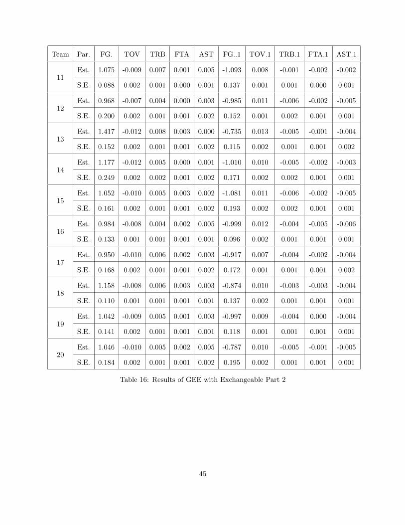
Table 16: Results of GEE with Exchangeable Part 2
45

Team Par. FG. TOV TRB FTA AST FG..1 TOV.1 TRB.1 FTA.1 AST.1
21Est. 0.994 -0.013 0.005 0.003 0.002 -1.154 0.013 -0.007 -0.002 -0.003
S.E. 0.122 0.002 0.001 0.001 0.001 0.137 0.001 0.001 0.001 0.001
22Est. 0.781 -0.007 0.001 0.004 0.006 -1.400 0.011 -0.008 -0.003 -0.002
S.E. 0.208 0.002 0.002 0.001 0.002 0.217 0.002 0.002 0.001 0.001
23Est. 0.810 -0.008 0.006 0.000 0.006 -0.889 0.003 -0.004 -0.004 -0.005
S.E. 0.121 0.001 0.001 0.001 0.001 0.117 0.002 0.001 0.001 0.001
24Est. 1.132 -0.011 0.005 0.002 0.003 -0.967 0.010 -0.006 -0.002 -0.003
S.E. 0.144 0.002 0.001 0.001 0.002 0.135 0.001 0.001 0.001 0.001
25Est. 0.767 -0.012 0.008 0.001 0.003 -1.012 0.011 -0.008 -0.003 -0.004
S.E. 0.140 0.002 0.002 0.001 0.001 0.185 0.002 0.001 0.001 0.001
26Est. 0.781 -0.012 0.003 0.002 0.002 -1.252 0.011 -0.008 0.000 -0.002
S.E. 0.169 0.002 0.001 0.001 0.002 0.153 0.001 0.002 0.001 0.002
27Est. 1.242 -0.010 0.006 0.003 0.004 -1.389 0.015 -0.004 -0.003 -0.003
S.E. 0.139 0.001 0.002 0.001 0.001 0.136 0.001 0.001 0.000 0.001
28Est. 0.647 -0.009 0.004 0.002 0.005 -1.193 0.010 -0.008 -0.002 -0.001
S.E. 0.134 0.001 0.001 0.001 0.001 0.134 0.001 0.001 0.001 0.001
29Est. 1.262 -0.012 0.006 0.002 0.004 -1.244 0.012 -0.003 -0.001 -0.003
S.E. 0.192 0.002 0.001 0.001 0.002 0.195 0.001 0.001 0.001 0.002
30Est. 1.070 -0.009 0.005 0.002 0.002 -1.161 0.010 -0.005 0.000 -0.004
S.E. 0.142 0.002 0.001 0.001 0.001 0.125 0.002 0.001 0.001 0.002
Table 17: Results of GEE with Exchangeable Part 3
Note that the standard errors in the above table are calculated with the robust sandwich
estimator.
46

Moreover, we will need to look at the correlation for each team, which is given in Table 18.
Team ID Correlation Team ID Correlation
1 0.354278784 16 -0.095566404
2 0.117149862 17 0.057239542
3 0.082767722 18 0.006081715
4 0.055304565 19 0.060014936
5 0.129417461 20 -0.044618320
6 0.247521718 21 -0.265618416
7 -0.032849678 22 -0.111676300
8 -0.060574930 23 0.055066874
9 0.077526727 24 -0.010043194
10 0.002991450 25 -0.026198157
11 -0.172255597 26 -0.007512587
12 0.162668762 27 -0.193221897
13 0.043981022 28 0.082928879
14 0.059295810 29 0.076284223
15 0.036479920 30 -0.167167453
Table 18: Correlation of exchangeable structure
47

For the AR-1 working correlation structure, which has the following form:
Corr(yit, yit′) =
1, t = t′
ρ|t−t′|, t 6= t′
the results are given in Tables 19, 20, and 21:
Team Par. FG. TOV TRB FTA AST FG..1 TOV.1 TRB.1 FTA.1 AST.1
1Est. 1.113 -0.008 0.006 0.002 0.005 -0.802 0.012 -0.006 0.000 -0.001
S.E. 0.137 0.001 0.001 0.001 0.001 0.158 0.001 0.001 0.001 0.001
2Est. 1.116 -0.010 0.005 0.003 0.002 -1.248 0.010 -0.004 -0.001 -0.001
S.E. 0.132 0.002 0.001 0.001 0.002 0.170 0.001 0.001 0.001 0.001
3Est. 0.766 -0.008 0.005 0.003 0.006 -1.060 0.007 -0.005 -0.001 -0.003
S.E. 0.154 0.001 0.001 0.001 0.001 0.126 0.001 0.001 0.001 0.001
4Est. 1.304 -0.009 0.006 0.001 0.005 -1.083 0.011 -0.004 -0.001 -0.005
S.E. 0.169 0.001 0.001 0.001 0.002 0.145 0.002 0.001 0.001 0.002
5Est. 1.135 -0.011 0.005 0.001 0.006 -1.215 0.010 -0.006 -0.004 -0.004
S.E. 0.170 0.002 0.001 0.001 0.002 0.157 0.002 0.001 0.001 0.002
6Est. 1.074 -0.009 0.004 0.004 0.004 -1.299 0.011 -0.005 -0.002 -0.004
S.E. 0.118 0.002 0.001 0.001 0.001 0.182 0.001 0.001 0.001 0.002
7Est. 1.294 -0.006 0.002 0.004 0.003 -1.296 0.008 -0.004 -0.002 -0.002
S.E. 0.249 0.002 0.001 0.001 0.003 0.160 0.002 0.001 0.001 0.001
8Est. 1.303 -0.011 0.003 0.003 0.002 -1.000 0.008 -0.005 -0.003 -0.004
S.E. 0.170 0.002 0.001 0.000 0.001 0.148 0.001 0.001 0.001 0.001
Table 19: Results of GEE with AR-1 Part 1
48

Team Par. FG. TOV TRB FTA AST FG..1 TOV.1 TRB.1 FTA.1 AST.1
9Est. 0.842 -0.009 0.005 0.002 0.005 -1.104 0.012 -0.008 -0.003 -0.003
S.E. 0.188 0.002 0.001 0.001 0.002 0.141 0.002 0.001 0.001 0.002
10Est. 1.119 -0.012 0.008 0.002 0.004 -1.097 0.011 -0.005 -0.003 -0.001
S.E. 0.111 0.001 0.001 0.001 0.001 0.161 0.002 0.001 0.001 0.002
11Est. 1.016 -0.009 0.007 0.002 0.006 -1.170 0.008 -0.001 -0.003 -0.002
S.E. 0.088 0.002 0.001 0.001 0.001 0.138 0.001 0.001 0.001 0.001
12Est. 0.953 -0.007 0.004 0.000 0.003 -0.989 0.011 -0.006 -0.002 -0.005
S.E. 0.201 0.002 0.001 0.001 0.002 0.157 0.001 0.002 0.001 0.001
13Est. 1.412 -0.012 0.008 0.003 0.000 -0.714 0.013 -0.005 -0.001 -0.004
S.E. 0.150 0.002 0.001 0.001 0.001 0.116 0.002 0.001 0.001 0.001
14Est. 1.233 -0.011 0.005 0.000 0.001 -0.943 0.010 -0.004 -0.002 -0.002
S.E. 0.279 0.002 0.001 0.001 0.002 0.184 0.002 0.002 0.001 0.001
15Est. 1.048 -0.009 0.005 0.003 0.002 -1.076 0.011 -0.006 -0.002 -0.005
S.E. 0.161 0.001 0.001 0.001 0.002 0.190 0.002 0.002 0.001 0.001
16Est. 0.993 -0.008 0.004 0.002 0.005 -1.014 0.011 -0.004 -0.005 -0.006
S.E. 0.135 0.001 0.001 0.001 0.001 0.099 0.002 0.001 0.001 0.001
17Est. 0.915 -0.010 0.006 0.002 0.003 -0.935 0.007 -0.004 -0.002 -0.004
S.E. 0.170 0.002 0.001 0.001 0.002 0.174 0.001 0.001 0.001 0.002
18Est. 1.153 -0.008 0.006 0.003 0.003 -0.873 0.010 -0.003 -0.003 -0.004
S.E. 0.109 0.001 0.001 0.001 0.001 0.138 0.002 0.001 0.001 0.001
19Est. 1.023 -0.009 0.005 0.001 0.003 -0.983 0.008 -0.004 0.000 -0.004
S.E. 0.141 0.002 0.001 0.001 0.001 0.119 0.001 0.001 0.001 0.001
Table 20: Results of GEE with AR-1 Part 2
49

Team Par. FG. TOV TRB FTA AST FG..1 TOV.1 TRB.1 FTA.1 AST.1
20Est. 1.014 -0.010 0.005 0.002 0.005 -0.812 0.010 -0.005 -0.001 -0.005
S.E. 0.181 0.002 0.001 0.001 0.001 0.197 0.002 0.001 0.001 0.001
21Est. 0.925 -0.013 0.005 0.003 0.002 -1.091 0.013 -0.006 -0.002 -0.004
S.E. 0.121 0.002 0.001 0.001 0.001 0.142 0.002 0.001 0.001 0.001
22Est. 0.772 -0.007 0.001 0.004 0.006 -1.439 0.011 -0.008 -0.003 -0.002
S.E. 0.198 0.002 0.002 0.001 0.002 0.214 0.002 0.002 0.001 0.001
23Est. 0.873 -0.008 0.005 0.001 0.006 -0.901 0.003 -0.004 -0.004 -0.004
S.E. 0.120 0.001 0.001 0.001 0.001 0.105 0.002 0.001 0.001 0.001
24Est. 1.147 -0.011 0.005 0.002 0.003 -0.999 0.010 -0.007 -0.002 -0.003
S.E. 0.142 0.002 0.001 0.001 0.002 0.140 0.001 0.001 0.001 0.002
25Est. 0.732 -0.012 0.007 0.001 0.003 -1.050 0.011 -0.008 -0.002 -0.004
S.E. 0.139 0.002 0.002 0.001 0.001 0.180 0.002 0.001 0.001 0.001
26Est. 0.726 -0.013 0.004 0.002 0.001 -1.293 0.011 -0.008 0.000 -0.001
S.E. 0.170 0.002 0.001 0.001 0.002 0.159 0.001 0.001 0.001 0.002
27Est. 1.251 -0.009 0.006 0.003 0.004 -1.420 0.014 -0.005 -0.002 -0.003
S.E. 0.146 0.001 0.001 0.001 0.001 0.128 0.001 0.001 0.000 0.001
28Est. 0.655 -0.009 0.004 0.002 0.005 -1.166 0.010 -0.008 -0.002 -0.001
S.E. 0.134 0.001 0.001 0.001 0.001 0.131 0.001 0.001 0.001 0.001
29Est. 1.327 -0.012 0.006 0.002 0.003 -1.289 0.012 -0.003 -0.001 -0.002
S.E. 0.192 0.002 0.001 0.001 0.002 0.190 0.001 0.001 0.001 0.002
30Est. 1.134 -0.010 0.006 0.001 0.002 -1.122 0.010 -0.004 0.000 -0.004
S.E. 0.148 0.002 0.001 0.001 0.001 0.139 0.002 0.001 0.001 0.002
Table 21: Results of GEE with AR-1 Part 3
Again the standard error is calculated using the robust sandwich estimator.
50

The correlation matrix has the following structure as in Table 22:
Team ID Correlation Team ID Correlation
1 0.39824344 16 -0.22744996
2 0.14450799 17 0.14767925
3 0.05763273 18 -0.02586013
4 0.20538148 19 0.02335451
5 0.18425673 20 0.14342430
6 0.23723676 21 0.38256248
7 -0.18705827 22 -0.29204104
8 0.04854666 23 0.20277552
9 0.09488453 24 0.19767212
10 -0.24567858 25 0.07939069
11 0.37705653 26 0.34888384
12 0.10818507 27 -0.26678847
13 -0.08906906 28 0.18495663
14 -0.22057998 29 -0.08486302
15 -0.06130218 30 -0.04838704
Table 22: Correlation of AR-1 structure
From Table 22, we can infer that this Within Team Correlation (first layer) yields a maximum of
less than 0.4 in terms of the absolute value.
Now, we will move onto the second layer, Between Team Correlation (BTC). For the moment, we
will assume the WTC is sufficiently small to ignore.
3.2.3 GEE Model and Working Correlation Matrix (in the Second Layer)
In this section, we will only consider the correlations between the games with one repeating team
involved and assume the correlations in the first layer to be zero.
Thus, we will put all the repeated games between two teams into one cluster, and the resulting
51

structure will be given in Table 23:
Team1 ID and Cluster Team2 ID
1
2
2
3
...
30
2
3
3
4
...
30
......
29 30
Table 23: Clusters for all teams
The games of team 30 (WAS) will be put into the previous clusters; thus, there will be no games
in cluster 30. Therefore, there will be only 29 clusters.
As the number of games decreases with the cluster index and this may place more emphasis on the
clusters with more observations, we will reverse the order of clusters and compare their results.
52

Estimate Robust S.E. Robust z P-Value
(Intercept) -0.0227 0.0309 -0.7363 0.4615
FG.1 1.0610 0.0364 29.1726 0.0000
TOV1 -0.0102 0.0004 -22.9781 0.0000
FTA1 0.0018 0.0003 6.9755 0.0000
TRB1 0.0052 0.0003 17.9060 0.0000
AST1 0.0042 0.0004 9.9566 0.0000
FG.2 -1.0741 0.0420 -25.5642 0.0000
TOV2 0.0106 0.0004 26.1595 0.0000
FTA2 -0.0019 0.0002 -7.8066 0.0000
TRB2 -0.0053 0.0003 -16.7662 0.0000
AST2 -0.0028 0.0004 -7.8934 0.0000
Table 24: Results from GEE of BTC with Exchangeable (Forward)
53

Estimate Robust S.E. Robust z P-Value
(Intercept) -0.0084 0.0437 -0.1918 0.8479
FG.1 1.0346 0.0425 24.3652 0.0000
TOV1 -0.0098 0.0004 -23.2022 0.0000
FTA1 0.0021 0.0002 9.1866 0.0000
TRB1 0.0052 0.0003 19.4058 0.0000
AST1 0.0036 0.0003 11.7466 0.0000
FG.2 -1.0604 0.0445 -23.8202 0.0000
TOV2 0.0104 0.0005 21.6446 0.0000
FTA2 -0.0018 0.0003 -6.0693 0.0000
TRB2 -0.0051 0.0004 -12.8730 0.0000
AST2 -0.0037 0.0003 -13.6718 0.0000
Table 25: Results from GEE of BTC with Exchangeable (Backward)
The correlation in Table 24 yields 0.0954 and the correlation in Table 25 yields 0.0921. We can
see that the difference in the estimations of the correlations are very small; thus, we can conclude
that there is no difference in the order of clusters with respect to exchangeable correlation structure.
The correlation is small in the model.
We can thus conclude that the BTC is sufficiently small to ignore and we will only take care of the
WTC.
3.2.4 Analysis of Within Team Pairs (First Layer)
In the previous section, we concluded that BTC can be neglected and WTC influences the proposed
GEE model much more. Now, we will analyze the WTC with the AR-1 working correlation.
Let us review the correlation structure of the WTC with AR-1 working correlation matrix. The
correlations given be each team is given in Table 26.
54

Team ID Correlation Team ID Correlation
1 0.39824344 16 -0.22744996
2 0.14450799 17 0.14767925
3 0.05763273 18 -0.02586013
4 0.20538148 19 0.02335451
5 0.18425673 20 0.14342430
6 0.23723676 21 0.38256248
7 -0.18705827 22 -0.29204104
8 0.04854666 23 0.20277552
9 0.09488453 24 0.19767212
10 -0.24567858 25 0.07939069
11 0.37705653 26 0.34888384
12 0.10818507 27 -0.26678847
13 -0.08906906 28 0.18495663
14 -0.22057998 29 -0.08486302
15 -0.06130218 30 -0.04838704
Table 26: Correlations of all teams
A higher correlation will give us more information in the games, so first, we will select all the
teams with a correlation higher than 0.2. These teams are those with team ids 1, 4, 6, 10, 11,
14, 21, 22, 23, 26, and 27. The corresponding names of the teams are given below. The last two
columns provide the information of their ranking and results of the 2017-2018 season, respectively.
55

Team id Correlation Team Name Results (Win-Lose) Ranking
1 0.3982 ATL 24-58 East 15
4 0.2053 CHI 27-55 East 13
6 0.2376 CLE 50-32 East 4
10 -0.2456 GSW 58-24 West 2
11 0.3770 HOU 65-17 West 1
14 -0.2205 LAL 35-47 West 11
21 0.3825 OKC 48-34 West 4
22 -0.2920 ORL 25-57 East 14
23 0.2027 PHI 52-30 East 3
26 0.3488 SAC 27-55 West 12
27 -0.2667 SAS 47-35 West 7
Table 27: Teams with highest correlations and their rankings
From Table 27 we can see that all these teams with a high correlation in their repeated games
are either the top teams or the teams with rather bad record. In Chapter 5, we will be predicting
the results of the playoff games, each round of which games are held in 7-game series between the
best 8 teams from each conference (Eastern and Western). Thus, the high correlations given by
these top teams will play their roles in the prediction of the playoff series.
In the last part of this chapter, we will consider only the WTC in the first layer and ignore the
BTW in the second layer to build the GEE model of the NBA game data.
The estimations of the ten parameters are given in Table 28.
56

Estimate Robust S.E. Robust Z P-value
FG.1 1.0604 0.0434 24.3775 0
TOV1 -0.0103 0.0004 -22.7218 0
TRB1 0.0052 0.0003 15.8110 0
FTA1 0.0019 0.0002 7.8552 0
AST1 0.0039 0.0004 9.2577 0
FG.2 -1.0434 0.0430 -24.2572 0
TOV2 0.0104 0.0004 24.0601 0
TRB2 -0.0052 0.0003 -16.7428 0
FTA2 -0.0020 0.0002 -8.6175 0
AST2 -0.0032 0.0003 -9.7317 0
Table 28: Estimations by GEE
All the factors are significant and thus the model will have the following form:
LG = −0.0167 + 1.06 ∗ FG.1− 0.0103 ∗ TOV 1 + 0.0052 ∗ TRB1 + 0.0019 ∗ FTA1 + 0.0039 ∗AST1
−1.0434 ∗ FG.2 + 0.0104 ∗ TOV 2− 0.0052 ∗ TRB2− 0.0020 ∗ FTA2− 0.0032 ∗AST2
4 Prediction of Factors
One fundamental consideration of the GEE model of the considered NBA game data is the per-
formance of the two teams involved in the considered games. To clarify, we first need to know the
performance of the two teams and then, we can build and train the proposed GEE model. This is
important for the coaches to understand the games from the unique perspective of data analysis.
However, this alone is not satisfactory as we also hope that we can predict the performance of teams
57

so that we cannot only have a sense of how a game in the future will look like based on the team’s
previous performance but also pay attention to some key statistics to improve the performance and
thus the team’s chances to win the game.
The factors to determine the performance of a certain statistic, taking the shooting percentage of
team 1 as an example, are the following:
• How well does team 1 perform in shooting?
• How well does the opposing team 2 perform in defending shooting?
• Is it a home game or an away game for team 1?
4.1 Prediction of Factors
Take the shooting percentage as an example. We assume that it consists of four parts, Shooting
Percentage Baseline, Offensive Score of the team, and Defensive Score of the opposition team and
whether the team has a home game or a game away from home.
FGTeami = Shooting-Baseline + Offensive-ScoreTeami + Defensive-ScoreTeamj + HA-Factor
The offense score and defense score for 30 teams for each factor will be estimated and they are
given in the following sections. Note that a high offense score infer that the team performs well for
the factor while a low defense score infer that the team performs well in lowering the opponent’s
performance for the factor (in another word, good defense performance).
58

4.1.1 Field Goal Percentage (FG)
The offense and defense scores for FG factor is given in Table 29 and Figure 12.
FG Scores
Team ID Offense Defense Team ID Offense Defense
1 -0.0131 0.0094 16 -0.0057 -0.0102
2 -0.0108 -0.0209 17 0.0181 0.0086
3 -0.0184 0.0054 18 0.0170 0.0153
4 -0.0249 0.0113 19 0.0232 -0.0054
5 -0.0102 0.0075 20 0.0036 -0.0027
6 0.0163 0.0139 21 -0.0080 -0.0033
7 -0.0155 0.0066 22 -0.0082 0.0075
8 0.0100 0.0153 23 0.0105 -0.0248
9 -0.0112 -0.0012 24 -0.0171 0.0100
10 0.0417 -0.0133 25 -0.0085 -0.0139
11 -0.0006 0.0020 26 -0.0098 0.0087
12 0.0120 0.0059 27 -0.0038 -0.0084
13 0.0119 -0.0016 28 0.0113 -0.0100
14 -0.0009 -0.0037 29 0.0010 -0.0117
15 -0.0168 0.0020 30 0.0068 0.0015
Base = 0.4561
Table 29: Scores for FG
59

Figure 12: FG. Offense vs FG. Defense
From Figure 12, the estimated FG scores (Offense and Defense) show how well a team performs
in FG factor. For a particular example, the Golden State Warriors (GSW) are one of the best
teams in both offense and defense of FG who lie in the bottom right corner, while the Chicago
Bulls (CHI) perform poorly on both ends who lie in the upper left corner.
4.1.2 Turnover (TOV)
The offense and defense scores for TOV factor is given in Table 30 and Figure 13.
60
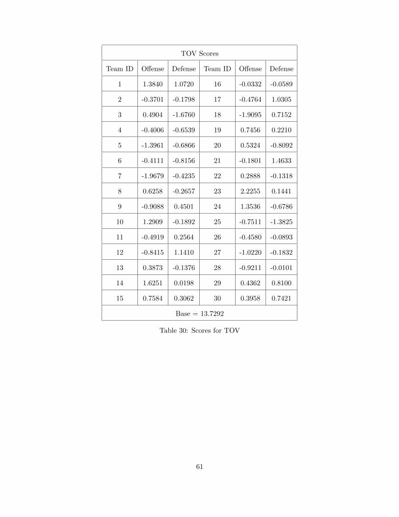
TOV Scores
Team ID Offense Defense Team ID Offense Defense
1 1.3840 1.0720 16 -0.0332 -0.0589
2 -0.3701 -0.1798 17 -0.4764 1.0305
3 0.4904 -1.6760 18 -1.9095 0.7152
4 -0.4006 -0.6539 19 0.7456 0.2210
5 -1.3961 -0.6866 20 0.5324 -0.8092
6 -0.4111 -0.8156 21 -0.1801 1.4633
7 -1.9679 -0.4235 22 0.2888 -0.1318
8 0.6258 -0.2657 23 2.2255 0.1441
9 -0.9088 0.4501 24 1.3536 -0.6786
10 1.2909 -0.1892 25 -0.7511 -1.3825
11 -0.4919 0.2564 26 -0.4580 -0.0893
12 -0.8415 1.1410 27 -1.0220 -0.1832
13 0.3873 -0.1376 28 -0.9211 -0.0101
14 1.6251 0.0198 29 0.4362 0.8100
15 0.7584 0.3062 30 0.3958 0.7421
Base = 13.7292
Table 30: Scores for TOV
61

Figure 13: TOV Offense vs TOV Defense
From Figure 13, the estimated TOV scores show how well a team performs in TOV factor. The
Philadelphia Sixers (PHI) yield the most turnovers per game and the Minnesota Timberwolves
(MIN) perform well in controlling the ball while forcing their opponents to make more mistakes.
4.1.3 Total Rebounds (TRB)
The offense and defense scores for the TRB factor is given in Table 31 and Figure 14.
62
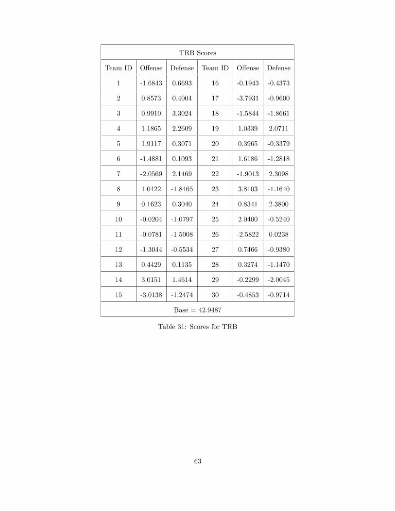
TRB Scores
Team ID Offense Defense Team ID Offense Defense
1 -1.6843 0.6693 16 -0.1943 -0.4373
2 0.8573 0.4004 17 -3.7931 -0.9600
3 0.9910 3.3024 18 -1.5844 -1.8661
4 1.1865 2.2609 19 1.0339 2.0711
5 1.9117 0.3071 20 0.3965 -0.3379
6 -1.4881 0.1093 21 1.6186 -1.2818
7 -2.0569 2.1469 22 -1.9013 2.3098
8 1.0422 -1.8465 23 3.8103 -1.1640
9 0.1623 0.3040 24 0.8341 2.3800
10 -0.0204 -1.0797 25 2.0400 -0.5240
11 -0.0781 -1.5008 26 -2.5822 0.0238
12 -1.3044 -0.5534 27 0.7466 -0.9380
13 0.4429 0.1135 28 0.3274 -1.1470
14 3.0151 1.4614 29 -0.2299 -2.0045
15 -3.0138 -1.2474 30 -0.4853 -0.9714
Base = 42.9487
Table 31: Scores for TRB
63

Figure 14: TRB Offense vs TRB Defense
From Figure 14, the estimated TRB scores show how well a team performs in TRB factor. The
Philadelphia Sixers (PHI) not only gain most rebounds per game but also provide less chance for
their opponents to gather rebounds. There are two main reasons for this phenomenon; Joel Embiid,
who is considered one of the best centers in the league; PHI performs well in the FG. and thus
provides less rebound chance for their opponents.
4.1.4 Free Throw Attempts (FTA)
The offense and defense scores for FTA factor is given in Table 32 and Figure 15.
64

FTA Scores
Team ID Offense Defense Team ID Offense Defense
1 -1.5227 -1.0961 16 -2.1021 1.3585
2 -1.1126 -0.2639 17 1.7896 1.9894
3 0.9355 1.9724 18 2.4680 -1.2431
4 -2.5052 -1.4246 19 -0.7516 -1.2714
5 5.1205 -3.0964 20 -2.7045 1.4828
6 1.4657 -2.0923 21 2.5552 -0.4305
7 -2.9716 -0.4865 22 -1.2568 -0.4247
8 0.6235 -1.2809 23 1.2009 4.0415
9 -2.1096 -2.7800 24 2.3852 2.8727
10 -1.2651 0.2352 25 -0.7485 0.1110
11 3.3712 -2.0363 26 -4.9418 -0.5096
12 -2.5518 -2.1753 27 -0.8557 -2.8611
13 3.9021 1.1162 28 0.2288 2.1249
14 1.6226 0.7267 29 -0.1142 -1.3963
15 -0.3130 4.9203 30 0.1580 1.9175
Base = 21.4113
Table 32: Scores for FTA
65

Figure 15: FTA Offense vs FTA Defense
From Figure 15, the estimated FTA scores show how many free throws a team get in a game.
The Houston Rockets (HOU) is one of the teams with most free throw attempts in a game, because
James Harden is so skillful in drawing fouls from opponents.
4.1.5 Assists (AST)
The offense and defense scores for AST factor is given in Table 33 and Figure 16.
66
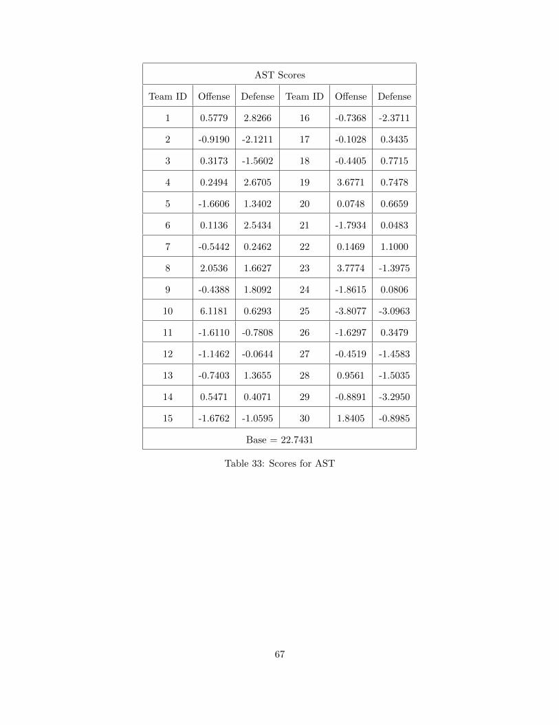
AST Scores
Team ID Offense Defense Team ID Offense Defense
1 0.5779 2.8266 16 -0.7368 -2.3711
2 -0.9190 -2.1211 17 -0.1028 0.3435
3 0.3173 -1.5602 18 -0.4405 0.7715
4 0.2494 2.6705 19 3.6771 0.7478
5 -1.6606 1.3402 20 0.0748 0.6659
6 0.1136 2.5434 21 -1.7934 0.0483
7 -0.5442 0.2462 22 0.1469 1.1000
8 2.0536 1.6627 23 3.7774 -1.3975
9 -0.4388 1.8092 24 -1.8615 0.0806
10 6.1181 0.6293 25 -3.8077 -3.0963
11 -1.6110 -0.7808 26 -1.6297 0.3479
12 -1.1462 -0.0644 27 -0.4519 -1.4583
13 -0.7403 1.3655 28 0.9561 -1.5035
14 0.5471 0.4071 29 -0.8891 -3.2950
15 -1.6762 -1.0595 30 1.8405 -0.8985
Base = 22.7431
Table 33: Scores for AST
67

Figure 16: AST Offense vs AST Defense
From Figure 16, the estimated AST scores show how many assists a team gather in a game.
The Golden State Warriors (GSW) perform so well in this factor for the sake of the basketball
philosophy of their coach is sharing the ball as much as possible.
5 Prediction of NBA Games with GEE Model
Now, we will combine the two stages and first predict the performance of the two teams and then,
use the predicted statistics to form our prediction of the winner of an NBA game in the future.
The proposed prediction model is trained with all the games prior to March 1, 2018. Thus, we will
first test on all the games after March 1. Some of the results are given in Tables 34 and 35.
68

Team1 Team2 True Ratio Predicted Ratio Winning Prediction
13 7 0.1941 0.0479 Correct
18 24 0.0969 0.0762 Correct
25 18 0.0870 0.0276 Correct
7 5 -0.0400 0.0195 Wrong
22 29 -0.3856 -0.0210 Correct
16 3 -0.2436 0.0372 Wrong
20 19 -0.0414 0.0038 Wrong
17 10 -0.1388 -0.0247 Correct
9 4 0.1762 0.0676 Correct
13 22 0.0734 0.0433 Correct
27 8 0.0190 0.0632 Correct
25 11 -0.0581 -0.0061 Correct
23 12 0.0953 0.0239 Correct
5 20 0.0679 0.0345 Correct
17 11 -0.1053 -0.0281 Correct
27 28 0.0404 0.0335 Correct
29 2 -0.0314 -0.0249 Correct
Table 34: Results of prediction part 1
Team1 Team2 True Result Predicted Result Winning Prediction
LAC DAL W W Correct
MIN PHO W W Correct
POR MIN W W Correct
DAL CHO L W Wrong
ORL UTA L L Correct
MIA BRK L W Wrong
NYK NOP L W Wrong
MIL GSW L L Correct
DET CHI W W Correct
LAC ORL W W Correct
SAS DEN W W Correct
POR HOU L L Correct
PHI IND W W Correct
CHO NYK W W Correct
MIL HOU L L Correct
SAS TOR W W Correct
UTA BOS L L Correct
Table 35: Results of prediction part 2
69

There are exactly 200 games in the test set, and the accuracy of the correct predictions is
68.45%. This is higher than the accuracy of all the methods in the previous work done by other
researchers [8] [9] [10].
Some explanations of the performance prediction are likely to improve from the following perspec-
tives. First, the games of some of the wrong predictions are fairly close games. The games between
DAL and CHO, and the game between NYK and NOP (from Tables 34 and 35), are examples
of such games. The difference between the scores of these two games are less than or equal to
5 points. These games can be decided by the last one or two possessions. Second, March is the
very last month of the regular season and some of the teams would like their starting players to
sit out in order to prepare for the playoff games. In this situation, the teams are likely to perform
quite differently from their previous performance and thus mislead in the prediction results. Third,
injuries start to hurt. The game between MIA and BRK (from Tables 34 and 35) is an example
where our false predicted winner, Miami Heats, had Justice Winslow (starting small forward) and
James Johnson (major rotation player) on the bench and not playing. In this game, MIA lost to
BRK even though MIA performed better in their previous games.
Now we should also test the accuracy of the proposed model with respect to the playoff games. We
will only predict the winner of each series. The structure of the playoff series is given in Figure 17.
There were 15 match-ups in total, and the prediction of each match-up is given in Table 36. The
proposed model yielded 12 correct predictions.
70

Figure 17: 2018 NBA Playoff Tree
71

Team1
(# of games win)
Team2
(# of games win)
True
Winner
Predicted
WinnerYes/No
First
Round
GSW (4) SAS (1) GSW GSW CORRECT
POR (0) NOP (4) NOP POR WRONG
HOU (4) MIN (1) HOU HOU CORRECT
OKC (2) UTA (4) UTA UTA CORRECT
BOS (4) MIL (3) BOS BOS CORRECT
PHI (4) MIA (1) PHI PHI CORRECT
CLE (4) IND (3) CLE CLE CORRECT
TOR (4) WAS (2) TOR TOR CORRECT
Conference
SemiFinal
GSW (4) NOP (1) GSW GSW CORRECT
HOU (4) UTA (1) HOU HOU CORRECT
BOS (4) PHI (1) BOS BOS CORRECT
TOR (1) CLE (4) CLE TOR WRONG
Conference
Final
HOU (3) GSW (4) GSW GSW CORRECT
BOS (3) CLE (4) CLE BOS WRONG
NBA Final GSW (4) CLE (0) GSW GSW CORRECT
Table 36: Results of prediction by GEE
72
For the three series that the GEE model yields a wrong prediction, there are two series involving
Cleveland Cavaliers (CLE). CLE did not perform as well in the regular season as they do in the
playoff games. In the series against Toronto Raptors (TOR), CLE lowered their opponent’s TRB
from 44.0 to 39.5, FTA from 21.8 to 18, and AST from 24.3 to 21.3. In their series against Boston
Celtics (BOS), CLE managed to lower their opponent’s FG. from 0.45 to 0.423, TRB from 44.5
to 40.4, and AST from 22.5 to 21.3. Thanks to the great performance increase in their defense,
CLE won both of the series. And due to the change in the performance, the GEE model fails to
prediction the winners. For the series between Portland Blazers (POR) and New Orleans Pelicans
(NOP), there are significant changes of performance. While NOP managed to increse their own
FG. from 48.3% to 52.2, POR’s TRB dropped from 45.5 to 43.5 and FTA from 20.9 to 15.75. NOP
won the series by the bouncing-back performance from their center/forward, Anthony Davis.
6 Conclusions and Outlook
In this dissertation, I worked on the NBA game data of the 2017-2018 season. The interesting point
of this data set was that we could assume that there is a correlation among the different games
(observations). Such correlation can only be drawn from the comparison with GEE model with
true correlation structure. This was observed from the experiment for the ordinary linear model
with two different cross validation methods.
For the GEE model, I examined two different working correlation structures, namely exchangeable
and AR-1. Both were reasonable for the considered NBA game data. From the estimated parame-
ters, I identified the most important factors in a game and how they influenced the results of the
games. These factors are: FG1, TOV1, TRB1, FTA1, and AST1 of team 1, and FG2, TOV2,
TRB2, FTA2, and AST2 of team 2. This is useful in helping teams improve their performance on
the court. Moreover, I observed that some teams had strong correlations between their games with
different opposition teams. This can be very helpful in the playoff games where the match-up will
perform in a seven-game series. In such situation, the GEE model will yield a better estimation of
73

the parameters since the GEE model takes the correlations between the games involving the same
match-ups into consideration. And our prediction of 2018 playoff series yields a accuracy of 80%.
Then, I predicted each of the factor in the GEE model. This would provide teams with a prediction
of how they could perform in a future game.
A combination of the two models above will help predict the winners of the games in the future
together with how the two teams are expected to perform. Thus, teams can adjust their lineups
and strategies to have the best chance to win the game.
The potential extensions to my dissertation can include but are not limited to the following: First,
find a more efficient working correlation structure for the GEE model, so that a more robust and
accurate estimation of the parameters can be revealed. Second, introduce a time trend in the pre-
diction stage, as the performance may also be influenced by the conditions of the players, which
could be a result of the time trend.
74

Bibliography
[1] A. Reifman, Hot Hand: The statistics behind sports’ greatest streaks. Potomac Books, Inc.,Dulles, 2011
[2] D. Oliver, K. Pelton, D. T. Rosenbaum, A starting point for analyzing basketball statistics JustinKubatko. Journal of Quantitative Analysis in Sports, doi 10.2202/1559-0410.1070
[3] J. Sampaio, M. Janeira, Statistical analyses of basketball team performance: Under-standing teams’ wins and losses according to a different index of ball possessions. doi10.1080/24748668.2003.11868273
[4] G. Csataljay, P. O’Donoghue, M. Hughes, H. Dancs, Performance indicators that distinguishwinning and losing teams in basketball. doi 10.1080/24748668.2009.11868464
[5] C. Puente, J.D. Coso, J. J. Salinero, J. Abian-Vicen, Basketball performance indicators duringthe ACB regular season from 2003 to 2013. doi 10.1080/24748668.2015.11868842
[6] J. Malarranha, B. Figueira, N. Leite, J. Sampaio, Dynamic modeling of performance in basket-ball. doi 10.1080/24748668.2013.11868655
[7] G. Csataljay, N. James, M. Hughes, H. Dancs, Effects of defensive pressure on basketball shootingperformance. doi 10.1080/24748668.2013.11868673
[8] J. Uudmae, Predicting NBA game outcomes. http://cs229.stanford.edu/proj2017/final-reports/5231214.pdf
[9] R. A. Torres, Prediction of NBA games based on machine learning methods.https://homepages.cae.wisc.edu/ ece539/fall13/project/AmorimTorres-rpt.pdf
[10] L. Hoffman, M. Joseph, A multivariate statistical analysis of the NBA.http://www.units.miamioh.edu/sumsri/sumj/2003/NBAstats.pdf
[11] Basketball-Reference. https://www.basketball-reference.com
[12] A. Ziegler, Generalized estimating equations. Springer Science+Business Media, LLC 2011,ISBN 978-1-4614-0498-9
[13] A. C. Rencher, G. B. Schaalje, Linear models in statistics. John Wiley Sons, Inc., Hoboken,New Jersey, ISBN 978-0-471-75498-5
[14] J. J. Faraway, Linear models with R. Taylor Francis e-Library, 2009, ISBN 1-58488-425-8
[15] C. R. Rao, H. Toutenburg, Linear models: Least squares and alternatives. Springer-Verlag NewYork, 1999,
[16] J. O. Rawlings, S. G. Pantula, D. A. Dickey, Applied regression analysis: A research tool.Springer-Verlag New York, 1998, ISBN 0-387-98454-2
[17] T. T. Kiang, K. Trivina, D. Hogan, Using GEE to model student’s satisfaction: A SASR© Macro Approach. Centre for Research in Pedagogy and Practice, Nanyang TechnologicalUniversity, Singapore (2009). Paper 251-2009 Practice, Nanyang
75

[18] J. W. Hardin, and J. M. Hilbe Generalized estimating equations. Boca Raton, FL: Chapmanand Hall/CRC Press, 2003
[19] J. D. Singer, J. B. Willet, Applied longitudinal data analysis. Modeling Change and EventOccurrence, 2003
[20] M. Stokes, C. Davis, G. Koch, Categorical data analysis using the SAS System. SAS Institute,Cary, N.C., 2000
[21] R. W. M. Wedderburn, Quasi-likelihood functions, generalized linear models, and the Gauss-Newton method. Biometrika, 1974
[22] A. Agreti, Categorical data analysis. Wiley, New York, 1990
[23] G. Box, D. R. Cox, An analysis of transformations. J R Stat Soc B, 26:211-252, 1964
[24] K. C. Li, N. Duan, Regression analysis under link violation Ann Stat, 17:1009-1052, 1989
[25] L. Y. Hin, Y. G. Wang, Working correlation structure identification in generalized estimatingequations. Stat Med, 28:642-658, 2009
[26] D. B. Hall, T. A. Severini, Extended generalized estimating equations for clustered data. J AmStat Assoc, 1998
[27] D. B. Hall, On GEE-based regression estimates under first moment misspecification. CommunStat - Theor M, 1999
[28] J. W. Hardin, J. M. Hilbe, Generalized linear models and extensions. Stata Press, CollegeStation, 2007
[29] S. L. Zeger, K. Liang and P. S. Albert, Models for longitudinal data: A generalized estimatingequation approach Biometrics 44, no. 4 (1988): 1049-060. doi 10.2307/2531734.
[30] G. A. Ballinger, Using generalized estimating equations for longitudinal data analysis. Organi-zational Research Methods, 7(2), 127–150,doi 10.1177/1094428104263672
[31] J. A. Hanley, A. Negassa, M. Edwardes, J. E. Forrester, Statistical analysis of correlated datausing generalized estimating equations: An orientation. American Journal of Epidemiology,Volume 157, Issue 4, 15 February 2003, Pages 364–375, doi 10.1093/aje/kwf215
[32] S. R. Lipsitz, N. M. Laird, D. P. Harrington, Generalized estimating equations for correlatedbinary data: Using the odds ratio as a measure of association. Biometrika, Volume 78, Issue 1,March 1991, Pages 153–160, https://doi.org/10.1093/biomet/78.1.153
[33] X. Lin, R. J. Carroll, Semiparametric regression for clustered data using generalized esti-mating equations. Journal of the American Statistical Association, 96:455, 1045-1056, DOI10.1198/016214501753208708
[34] S. R. Lipsitz, G. M. Fitzmaurice, E. J. Orav, N. M. Laird. Performance of generalized estimat-ing equations in practical situations. Biometrics 50, no. 1 (1994): 270-78. doi 10.2307/2533218.
[35] T. Lumley, Generalized estimating equations for ordinal data: A note on working correlationstructures. Biometrics 52, no. 1 (1996): 354-61. doi 10.2307/2533173.
76