Modeling of Mixing in The Liquid Phase For Bubble Column

Eng. & Tech. Journal, Vol.27, No.10, 2009

*Material Engineering Department, University of Technology/Baghdad 1992

Modeling of Mixing in The Liquid Phase For Bubble

Column

Dr.Ali H. Jawad* Received on:10/11/2008

Accepted on:5/3/2009

Abstract Hydrodynamic characteristics (mixing in the liquid phase) in a bubble column with a non-Newtonian liquid phase (aqueous solutions of carboxymethylcellulose, or CMC, at different concentrations) were measured and correlated. Experiments in a 0.2-m diameter, 2.4-m-high bubble column were carried out to determine degree of mixing in the liquid phase at various gas and liquid flow rates. The axial dispersion model was used in the two operating modes, batch and continuous, and the tanks-in-series model was used just in the case of continuous mode. The axial dispersion model with closed-closed boundary conditions fit experimental data quite well and thus was used to estimate the axial dispersion coefficient. This parameter was higher in batch mode than in continuous mode, and its trend was to increase as superficial gas velocity increased.

Keywords: Bubble column, Non-Newtonian, Mixing in liquid phase, CSTR reactor, PFRreactor, Tank-in-series model and the dispersion model.

لعمود الفقاعيالسائل للطور للخلط في يةذجونم الخلاصة

الفقاعي للسوائل النيوتينة الغير القابلةفي عمود ) الاختلاط في المرحلة السائلة(الهيدرودينامية الخصائص اما بالنسبة .حسابها رياضيا وها ، تم قياس) بتراكيز مختلفةCMC اوcarboxymethylcellulose (لانضغاط

فقاعة أجريت لتحديد درجة من /عمودال مترا ارتفاع 2.4 و مترا وقطره0.2 في أجريت لجانب العملي . الغاز و السائلمن ةتدفق مختلف معدلات الاختلاط في المرحلة السائلة في

، (Continuous) ومستمرة(Batch) المستخدم في تشغيل اثنين من وسائط ، دفعةموديل التشتت الافقيتظام مع موديل التشتت الافقي. نموذج فقط في حالة طريقة مستمرة استخدم (Series) في سلسلةالخزان و

ن المستخدمة لتقدير معامل البيانات التجريبية ، وبالتالي كامع الظروف تناسب تماما في اغلاق-اغلاق ، (Continuous) من طريقة في طريقة مستمرة(Batch) كانت أعلى في دفعةالقيم هذه . التشتت محوري

.والاتجاه إلى زيادة سطحية كما زادت سرعة الغاز

PDF created with pdfFactory Pro trial version www.pdffactory.com

http://www.pdffactory.com


Eng. & Tech. Journal, Vol.27,No.10, 2009 Modeling of Mixing in The Liquid

Phase For Bubble Column

1993

Introduction

Many models can be used to

describe bubble column reactors.

Some aspects to take into account

when it is proposed a model are the

mathematical nature of the equations

and the degree of complex of their

solution (Deckwer, 1992).

The liquid phase mixing has

an important effect on mass transfer

capabilities of bubble column. Mixing

in bubble columns is due to liquid

circulation caused by the rise of the

bubbles through liquid phase, reducing

or eliminating the concentration

gradient, in the system. Because of the

high ratio of length to diameter, the

radial gradients are often neglected

compared to axial gradients (Walter

and blanch, 1983).

Several mathematical models

have been proposed in the literature to

describe mixing based on conservation

laws or simply based on empirical

relations. It is common to use an

injection of a tracer at the feed and

then measure tracer concentrations at

the exit. These collected data are

analyzed using, for example, the

moment's theory or the transfer

function of a mathematical model that

could represent the behavior of these

experimental data. The disadvantage

of the moments method is that

moments can be quite sensitive to

measurement errors at the tail of the

function E(t), (Ostergaard and

Michelsen, 1969). In the case of

bubble columns, mixing or back

mixing of each phase (degree of

turbulence) is due to flow or

movement of the fluids through the

column.

The rising bubbles cause turbulent

stochastic diffusion processes and

large-scale steady circulation flows

(Riquarts, 1981).

Theory

Some of the mathematical

models found in literature are

presented in this section.Models as

perfect mixing (CSTR), partial mixing

(ADM) and tubular flow (PFR) may

be found in gas and liquid phases

operations (Deckwer, 1992).






1994

1-Continuous, Stirred-Tank Reactor

(CSTR)

The continuous-stirred-tank

reactor is a perfectly mixed tank with

steady-state inlet and exit flow

streams. Therefore, the concentration

in the reactor, c(t), is only function of

time. The expression obtained from a

mass balance for an impulse of tracer

is (Froment and Bischoff, 1979 :)

….. (1)

where is the mass of tracer added

initially as an impulse, V is the fluid

volume in the tank (considered

constant), t is the time and, is

the exit concentration of the tracer,

which is the same as the concentration

inside the reactor at the any particular

time, and is the residence time

defined as the relation between reactor

volume, V and volumetric flow rate of

the feed, Q.

The Eq. (1) can be expressed in terms

of the age distribution function as:

…….(2)

For a step injection, the solution of the

tracer mass balance, for a zero initial

concentration in the system is:

... (3)

Where is the input

concentration for t ≥ 0. When a step

injection is used, the cumulative

function F(t) is used instead of the

distribution function E(t), and the

resulting expression for a continuous

stirred tank is:

F(t)= 1- exp (-t/ ) ………... (4)

2 Plug-Flow Reactors (PFR)

In an ideal, plug-flow reactor

(considered tubular), the fluid is

assumed to travel through the system

at uniform velocity and in straight

streamlines; therefore there are no

radial concentration gradients. Under

these conditions, the concentration in

the reactor, c(t,z), is a function of time

and axial position in the reactor. A

tracer mass balance on a differential

element of fluid inside the reactor,

taking into account as initial condition,






1995

c(0,z) = 0 in the case of an impulse

injection, gives the final expression:

…… (5)

Where L is the exit point (i.e., the

length of the reactor).

In case of a step injection, the exit

concentration will be given by:

…….. (6)

Where is the maximum

concentration that corresponds to feed

concentration of tracer and H(t) is the

Heaviside function that gives the step

form of the obtained answer.

3 Tank-in-Series Model

This model is a modified

CSTR model, where a mass balance of

the tracer is made in a generic tank "n"

of a series of identical tanks that

constitute the system. When the

resulting equation from the mass

balance is manipulated and the initial

and the boundary conditions are

applied, the final expression is

obtained for each form of tracer

injection:

For step injection tests (Levenspiel,

1999):

…(7)

Where N is the number of tanks in the

system.

For impulse injection tests (Froment

and Bischoff, 1979):

….. (8)

The plots of equation (7) and (8) are

presented by Levenspiel (1999) and

they are shown in figures (1) and (2)

respectively.

4 The dispersion model

The dispersion model is used to

describe tubular non-ideal reactors. It

considers that there is a Fickian

dispersion of matter, i.e., described by

a constitutive equation similar to the

Fick' s law of diffusion. The

expression of the model results from a

-tracer mass balance considered that is

injected at the feed of the system. The

model takes into account two effects:

convection, which represents the bulk

flow, and dispersion, which results

from the molecular and turbulent






1996

diffusion. There are two types of

contributions to dispersion: radial and

axial (Riquarts, 1981). The radial

effect is negligible in comparison to

axial effect when the aspect ratio L/D

is greater than 4. The model is then

called axial-dispersion model. In this

case, the concentration c(t,z) is a

function of time and axial position in

the reactor, and it is described by the

following expression:

…..(9)

Where c is the concentration of the

trace, u the fluid velocity, Dz the axial

coordinate, and t the time. This

equation can be written in

dimensionless from:

…..(10)

Where the new variables are defined

as:

……..(11)

……..(12)

……..(13)

……..(14)

Where L is the characteristic length (in

this case, the length of the reactor) and

Boz is the bodenstein number in the

axial direction. For simplicity, the

Bodenstein number will be expressed

as Bo instead Boz.

The Bodenstein number is the ratio of

transport rate by convection to the

transport rate by dispersion. The

inverse of the Bodenstein number is

called dispersion number.

The solution to the differential

equation on the boundary conditions

are needed, one at z=o the injection

point, and one at z=l the point at which

the response is measured each

condition depends on whether there is

dispersion before the injection (z=0)

and after the response point (z=L) If

there is dispersion on both sides of any

these points, it is an open boundary;

otherwise it is called a closed

boundary. Combinations are possible

for a reactor open-open, open –closed,

closed –open and closed –closed

boundaries result in a mathematical






1997

discontinuity in concentration by a

discontinuity in dispersion.

When open –open boundary

conditions are used, they can be

written as:

The corresponding analytical solution

of equation (10) at z*=1 is (Froment

and Bischoff, 1979):

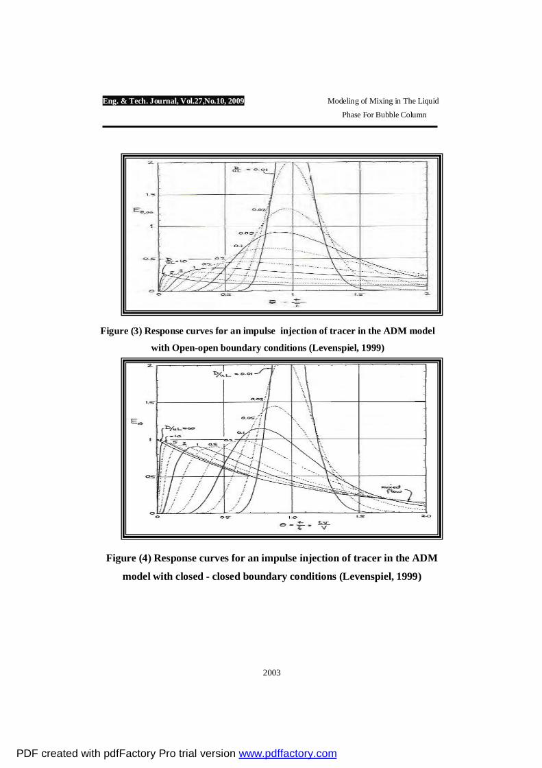
…..(15)

And the response curves for an

impulse injection is shown in figure

(3)

On the other hand, the following

closed-closed boundary conditions,

normally called Danckwerts boundary

conditions, may be used

and the corresponding analytical

solution at z* = 1 is (Froment and

Bischoff, 1979):

…….(16)

Where the Eigen values of this

series solution are the roots of the

following equation:

.. (17)

Figure (4) shows the response curves

for impulse injection of tracer in these

boundary conditions.

On the other hand, when there are at

least two phases in the system, the

equation (9) needs to be modified as

follows:

……..(18)

Where c is the tracer concentration in

the Liquid phase.

When figures 2 through 4 are

compared, the trends of figures 2 and 4

are similar because both models

consider that the mixing is inside the

system and in enter and exit zones

there are not mixing.






1998

Many researchers have studied the

back mixing in bubble columns

showing the dependence on the

column diameter, gas distributor, and

gas velocity, but the influence of the

velocity and properties of the liquid

phase on the mixing of the same

phase, especially when the liquid

phase is non-Newtonian is not known.

Some experimental and mathematical

works are described below.

Ohki and Inoue (1970) determined

longitudinal dispersion coefficient in

batch bubble column with 0.04, 0.08

and 0.16 m diameters. They stated that

the one - dimensional diffusion

model is valid when the distance

between injection tracer and

measuring points are sufficiently long.

They use the one-dimensional

diffusion model resulting from Eq. (9)

when the convective term is neglected:

...... (19)

The boundary conditions used by

authors are:

While the initial condition is:

Where p is a height filled with tracer.

The solution to the differential

equation is:

….(20)

Where CE is related through the

expression:

...... (21)

The researchers determined the

dispersion coefficient from the

expression:

......... (22)

DZ is obtained from the fitting of Eq.

(20) to experimental data, where the

authors plotted c/ cE as a function of

and took as the

distance in the abscise marked when

the value of c/ cE = 0.7 and c/ cE = 0.3

intercept the curve obtained from the

model for a z/ L. The authors

correlated the data and proposed two






1999

expressions that depend on prevailing

flow regime:

Homogeneous regime:

……. (23)

Slug flow regime:

…. (24)

They got agreement of the proposed

expression with experimental data.

Experimental

The experimental setup is

shown in Figure (5).

The main components are: a column

made up by two cylindrical sections of

Plexiglas of 0.20 m of inner diameter

and an entrance

cone, a self-metering pump, two

plastic feed tanks, filter devices, a

rotameter to measure the gas flow rate,

and a pressure transducer connected to

a data acquisition system.

Two types of experiments were carried

out: continuous (the gas and liquid

phases are fed continuously in the

column in the bottom of the column,

flowing in this case in ascendant and

cocurrent mode) and semicontinuos

modes (the gas phase flow in

ascendant mode while the liquid phase

was charged to the column at the

beginning of the operation). First the

CMC solution was prepared in one of

the feed tanks. Runs were carried out

at various gas and liquid superficial

velocities and at various

concentrations of CMC.

Aqueous solutions of

carboxymethylcellulose (provided by

Noviant) at different concentrations,

which are known to exhibit non-

Newtonian behavior, were used in the

experiments.

exit concentrations of tracer in the

residence time distribution

experiments were analyzed through

the axial dispersion model and tank-in-

series model using the moment theory

and direct fit of the experimental data

to the model. As a result of this

procedure, the number of tanks in

series, Bodenstein number and axial

dispersion coefficient in the liquid

phase were found, taking into account

the multiphase system used in this case






2000

(gas and liquid phases involved in the

experiments). Axial dispersion

coefficient data were correlated for

each flow regime as a function of

superficial velocities of gas and liquid

phases, and rheological parameters of

the power-law model.

Results and discussion

This section. Additionally, the fit

of experimental data by a proposed

correlation through the minimization

of the sum of squares of errors using a

Mathcad @ subroutine is presented,

together with the best estimate of the

parameter and the moments calculated

from the parameter. Figure (6) shows

there is not a significant difference in

the exit-tracer concentration between

the two radial positions; therefore, it is

reasonable to consider only the effect

of axial position in the dispersion

model.

The mixing in the liquid phase was

studied considering the operation

mode. In each case (batch and

continuous mode), experimental data

and the equation of the model

considered could fit these data were

plotted. The parameter of the proposed

model was adjusted to find its best

value that permitted the best fit. This

procedure was developed through

Mathcad® software and its

minimization technique.

In the case of batch mode, the

programmed expression was Eq. (20)

and the results of this model shows

that it fitted quite well experimental

data as it is observed in Figure (7) for

tap water. Similar plots are shown in

Figures (8) and (9) for 0.20 and 0.40%

CMC solutions.

In continuous mode, Eq. (8) for the

tanks-in-series model and Eq. (15) for

the axial dispersion model with

boundary conditions open-open were

programmed in Mathcad®.

Figure (10) shows the experimental

data and the models tested for tap

water. It is observed that the axial

dispersion model (ADM) with open-

open boundary conditions does not fit

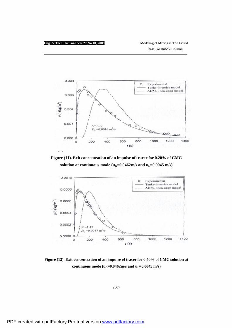
the experimental data. Figures (11)

and (12) show results for 0.20 and

0.40% CMC solutions that were

similar to those obtained with tap






2001

water. These results were similar at the

other gas and liquid superficial

velocities considered

Conclusions

In the bubble column, no

changes in the concentration curves at

the same operating conditions were

found at different radial positions.

The dispersion model for semi

continuous mode fit quite well

experimental data and tanks-in-series

model fit well experimental data for

continuous mode. The calculations of

the axial dispersion coefficient from

the model with closed-closed

boundary conditions showed

consistency in the expressions of the

three moments derived for this model.

The axial dispersion model with open-

open boundary conditions did not fit

experimental data.

Axial dispersion coefficient exhibited

higher values in the batch mode than

in continuous mode. References

[1] Deckwer, W.D. Bubble Column

Reactors, John Wiley & Sons. New

York. pp.533. (1992).

[2] Froment, G. and Bischoff, K.,

Chemical Reactor Analysis and

Design, John Wiley & Sons. New

York. pp.764. (1979).

[3] Levenspiel, O., Chemical Reaction

Engineering, 3rd edition, John Wiley &

Sons, pp.668 (1999).

[4] Ohki, Y. and Inoue, H.,

"Longitudinal mixing of the liquid

phase in bubble columns", Chern. Eng.

Sci., 25, 1-16 (1970).

[5] Ostergaard, K. and Michelsen,

M.L., "On the use of the imperfect

tracer pulse method for determination

of hold-up and axial mixing," The

Canadian J. of Chern. Eng., 47, 107

(1969).

[6] Riquarts H.-P., "A physical model

for axial mixing of the liquid phase for

heterogeneous flow regime in bubble

columns," Ger. Chem. Eng., 4, 18-23

(1981).

[7] Walter, J. F., and Blanch, H. W.

"Liquid circulation patterns and effect

on gas hold-up and mixing in bubble

columns," Chem. Eng. Commun.,

19,243-262 (1983).






2002

Figure (1) Response for a step injection of tracer in

the tanks-in-series model (Levenspiel, 1999)

Figure (2) Response for an impulse injection of tracer in

the tanks-in-series model (Levenspiel, 1999)






2003

Figure (3) Response curves for an impulse injection of tracer in the ADM model

with Open-open boundary conditions (Levenspiel, 1999)

Figure (4) Response curves for an impulse injection of tracer in the ADM

model with closed - closed boundary conditions (Levenspiel, 1999)






2004

Figure (5) Experimental setup

Figure (6) Exit-tracer concentration for tap water in continuous mode

(uG=0.0112 m/s and uL=0.0017 m/s) at two radial positions

t(s)

c(t)

(Kg/

m3 )*

10-4

-1

0

1

2

3

4

5

6

7

-200 200 600 1000 1400 1800 2200 2600 3000

r=0r=R/2






2005

Figure (7). Exit-tracer concentration for tap water in batch

mode (uG=0.0083m/s and uL=0 m/s)

Figure (8) Exit-tracer concentration for 0.20% CMC

solution in batch mode (uG=0.0308m/s and uL=0 m/s)

t(s)

c(t)

(Kg/

m3 )*

10-4

0

2

4

6

8

10

0 40 80 120 160 200

Exxperimental Model

t(s)

c(t)

(Kg/

m3 )*

10-4

0

1

2

3

4

5

6

0 100 200 300 400 500

Experimental Model






2006

Figure (9). Exit-tracer concentration for 0.40% CMC

solution in batch mode (uG=0.462m/s and uL=0 m/s)

Figure (10). Exit concentration of an impulse of tracer for tap

water at continuous mode (uG=0.0010 m/s and uL=0.0025 m/s)

t(s)

c(t)

(Kg/

m3 )8

10-4

-1

1

3

5

7

9

11

-50 50 150 250 350 450 550

ExperimentalModel






2007

Figure (11). Exit concentration of an impulse of tracer for 0.20% of CMC

solution at continuous mode (uG=0.0462m/s and uL=0.0045 m/s)

Figure (12). Exit concentration of an impulse of tracer for 0.40% of CMC solution at

continuous mode (uG=0.0462m/s and uL=0.0045 m/s)




Modeling of Mixing in The Liquid Phase For Bubble Column

Documents

Transcript of Modeling of Mixing in The Liquid Phase For Bubble Column