
Modeling of cohesive crack growth in partially saturated ... · As the fracture mechanics–based...
39
1 Submitted to: International Journal of Fracture Revised version: FRAC 1439 Modeling of cohesive crack growth in partially saturated porous media; A study on the permeability of cohesive fracture O.R. Barani , A.R. Khoei * and M. Mofid Center of Excellence in Structures and Earthquake Engineering, Department of Civil Engineering, Sharif University of Technology, P.O. Box. 11365-9313, Tehran, Iran Abstract Modeling the water flow in cohesive fracture is a fundamental issue in the crack growth simulation of cracked concrete gravity dams and hydraulic fracture problems. In this paper, a mathematical model is presented for the analysis of fracture propagation in the semi-saturated porous media. The solid behavior incorporates a discrete cohesive fracture model, coupled with the flow in porous media through the fracture network. The double-nodded zero-thickness cohesive interface element is employed for the mixed mode fracture behavior in tension and contact behavior in compression. The modified crack permeability is applied in fracture propagation based on the data obtained from experimental results to implement the roughness of fracture walls. Keywords. Fracture propagation; Porous media; Partially saturated; Cohesive fracture; Fracture permeability. * Corresponding author. Tel. +98 (21) 6600 5818; Fax: +98 (21) 6601 4828. Email address: [email protected] (A.R. Khoei)
Transcript of Modeling of cohesive crack growth in partially saturated ... · As the fracture mechanics–based...

1
Submitted to: International Journal of Fracture Revised version: FRAC 1439
Modeling of cohesive crack growth in partially saturated
porous media; A study on the permeability of cohesive
fracture
O.R. Barani , A.R. Khoei
* and M. Mofid
Center of Excellence in Structures and Earthquake Engineering, Department of Civil Engineering,
Sharif University of Technology, P.O. Box. 11365-9313, Tehran, Iran
Abstract
Modeling the water flow in cohesive fracture is a fundamental issue in the crack growth simulation
of cracked concrete gravity dams and hydraulic fracture problems. In this paper, a mathematical
model is presented for the analysis of fracture propagation in the semi-saturated porous media. The
solid behavior incorporates a discrete cohesive fracture model, coupled with the flow in porous
media through the fracture network. The double-nodded zero-thickness cohesive interface element
is employed for the mixed mode fracture behavior in tension and contact behavior in compression.
The modified crack permeability is applied in fracture propagation based on the data obtained from
experimental results to implement the roughness of fracture walls.
Keywords. Fracture propagation; Porous media; Partially saturated; Cohesive fracture; Fracture
permeability.
* Corresponding author. Tel. +98 (21) 6600 5818; Fax: +98 (21) 6601 4828.
Email address: [email protected] (A.R. Khoei)
2
1. INTRODUCTION
Modeling the water flow in cohesive fracture propagation plays the main role in the crack growth
simulation of porous saturated media. The hydraulic fracture problem and cracked concrete gravity
dams normally have cracks in practical service due to previous earthquakes, construction
conditions, or temperature effects. For a concrete dam subjected to its probable maximum flood, it
is speculated that the hydrostatic pressure acting inside the crack induces additional material
damage and hence, reduce the resistance against further cracking which can lead to the weakness of
structure and the penetration of water that exerts uplift pressure (Rescher 1990; Zhu and Pekau
2007). The study of crack propagation in concrete dams can be performed based on the development
of interface models in poroelastic material.
Modeling of discontinuities between two bodies in contact has been performed by contact
elements in computational solid mechanics. The idea has been used to model the cohesive forces via
the cohesive elements in numerical fracture mechanics (Ortiz and Suresh 1993; Xu and Needleman
1994). The double-nodded zero-thickness interface element was used by Ng and Small (1997) in flow
problems. Segura and Carol (2004) proposed the influence of transversal conductivity with the aim
of applying these elements in the hydro-mechanical problems. Simoni and Secchi (2004)
implemented the double-nodded interface elements in quasi-static fracture propagation of saturated
porous media. The technique was proposed by Schrefler et al. (2006) and Secchi et al. (2007) based
on an adaptive mesh refinement in porous materials. The cohesive crack growth was performed by
Khoei et al. (2009b) using the adaptive FE strategy in the framework of cohesive interface elements.
A new formulation was developed for double-nodded interface elements by Khoei et al. (2009a) in
the dynamic fracture propagation of saturated porous media, in which a new transversal
conductivity relation was introduced.
As the fracture mechanics–based analysis is being increasing accepted as an analytical and
numerical tool for cracked massive concrete structures, the fracture properties must be defined
appropriately according to experimental data. Brühwiler and Saoma (1995a, b) conducted a series of
experimental studies to determine that the static pressure inside a crack is a function of crack
opening and that, along the fracture process zone, this pressure reduces from full reservoir pressure
to zero. Reinhardt et al. (1998) investigated the flow in concrete cracks and concluded that the
permeability of cracks having an opening more than about 0.04 mm is higher than the undamaged
concrete. For smaller crack widths the penetration behavior is similar to that of uncracked concrete.
Slowik and Saouma (2000) developed an experimental and numerical investigation on the influence
of water pressure on crack propagation in concrete. From the experimental results they pointed out

3
that the crack opening rate significantly influences the water pressure distribution. On the basis of
experimental results they proposed an interface model, considering the fluid permeability as a
function of crack opening displacements. However they did not consider the compressibility of
solid and fluid and also the roughness of fracture walls as a key parameter of fracture permeability.
That is a general assumption for the concrete material that a properly cured concrete or an
underwater concrete is fully saturated by water. Persson (1997) indicated that the relative humidities
inside concrete samples are lower than 100% even though the samples were stored under water
indicating unsaturated states of concrete. It was shown that the relative humidity could be about
0.77 even after 450 days under water curing.
In the present paper, a finite element algorithm was presented for the numerical modeling of
cohesive fracture in a partially saturated porous media. The double-nodded zero-thickness cohesive
interface elements were employed to capture the mixed mode fracture behavior in tension and
compression. In order to describe the behavior of fractured media, two equilibrium equations were
applied similar to those employed for the mixture of solid-fluid phase in semi-saturated media,
including: the momentum balance of fractured media, and the balance of fluid mass within the
fracture. Based on the experimental data performed by Slowik and Saouma (2000), a modified crack
permeability is introduced to model the roughness of fracture walls.
2. FE FORMULATION OF SEMI-SATURATED POROUS MEDIA
The mathematical formulation governing the behavior of dynamic saturated porous medium was
first introduced by Biot (1941). The first numerical solution for these equations was made by
Ghaboussi and Wilson (1973). A simple extension of two phase formulation to semi-saturated
problems was proposed by Zienkiewicz et al. (1990) based on the assumption of the air or gas present
in the pores remaining at atmospheric pressure. They employed their extended formulation for the
dynamic analysis of a semi-saturated dam under earthquake loading. The coupled formulations that
involve the air and water phases in a porous medium have been presented by Alonso et al. (1990) and
Gawin and Schrefler (1996). However, because of great complexity of three-phase models, an
extensive and special designed testing is required to determine the properties of the matrix–air–
water mixture.
In the theory of porous media, the effective stress is an essential concept for the deformation of
solid skeleton. The effective stress ijσ ′ can be defined by wwijijij pSαδσσ −=′ , in which
ijδ denotes
4
the Kronecker delta and ijσ and wp are the total stress and water pressure, respectively, with
positive value in compression. In this relation, α is the Biot coefficient which depends on the
material type and defined as 1 T sK Kα = − , with T
K and s
K denoting the bulk modulus of porous
medium and solid particles, respectively. wS is the water saturation, defined as a function of the
water pressure, i.e. )( www pSS = . Note that for the saturated porous media, the water pressure is
assumed to be positive and the effective stress is less than the total stress, while for the partially
saturated porous medium when the gas pressure is close to zero, the water pressure is negative and
the effective stress is more than the total stress.
The linear momentum balance for the mixture of solid-fluid phase can be written as
0, =−+ iijij bu ρρσ && (1)
where ib is the body force per unit mass and ρ indicates the density of total mixture defined by
sww nnS ρρρ )1( −+= , with wρ denoting the water density, sρ the density of solid particles, and n
the porosity.
Incorporating the Darcy law, the mass balance for the fluid phase can be written as
( ), *,( ) 0w
rm ij w j w j w j w iii
pk k p u b S
Qρ ρ α ε+ − + + =
&&&& (2)
where iiε is the total volumetric strain, ijk the permeability tensor of the medium,
rmk the relative
permeability of the matrix which is a function of the water pressure, i.e. )( wrmrm pkk = , and *Q is
defined as
)()(1
* ws
w
s
w
w
ws p
n
CS
K
Sn
K
SnC
Q+−++= α (3)
where wK denoting the bulk modulus for liquid phase and sC the specific moisture content defined
as w wn dS dp (Zienkiewicz et al. 1999).
The governing equations (1) and (2) can be discretized for quasi-static problems in the absence
of acceleration terms by using two sets of shape functions uN and pN for two variables iu and wp ,
defined as u=u N u and w p wp p= N , based on the standard Galerkin technique to transform these
equations into a set of algebraic equations as (Khoei et al. 2004)

5
(1)
wp− =Ku Q f (4)
(2)
w wp p+ + =Qu H G f& & (5)
where the stiffness matrix K , the coupling matrix Q , the permeability matrix H , and the
compressibility matrix G are defined as
*
1
T
T
w p
T
p rm p
T
p p
d
S d
k d
dQ
α
Ω
Ω
Ω
Ω
= Ω
= Ω
= ∇ ∇ Ω
= Ω
∫
∫
∫
∫
K B D B
Q B m N
H N k N
G N N
(6)
and
(1)
(2) ( )
t
q
T T
u u
wT T T
p rm w p
w
d d
qk d d
ρ
ρρ
Ω Γ
Ω Γ
= Ω+ Γ
= − ∇ Ω+ Γ
∫ ∫
∫ ∫
f N b N t
f N k b N
(7)
where B is the matrix relating the increments of strain and displacements, D is the material
property matrix of solid skeleton, and m is defined as [1, 1, 0, 1]T=m (Khoei et al. 2006). In above
relations, Ω is the domain of fluid and solid fields, tΓ is the external boundary for traction, qΓ is
the external boundary for influx, and wq is the imposed flux on qΓ . The permeability matrix k is
defined as
=
yyx
xyx
kk
kkk (8)
where xk and yk are the permeability coefficients in x and y directions, respectively, and xyk and
yxk are generally set to zero.
Based upon the pore network model, a relationship between the capillary pressure and the water
saturation is proposed by van Genuchten (1980) as

6
1 (1 )
( ) 1
mm
ww w
r
pS p
p
−− = +
(9)
in which the reference pressure rp and the coefficient m are defined based on the experimental
data obtained by Baroghel-Bouny et al. (1999) as 18.6237 MParp = and 4396.0=m , respectively.
The relative permeability is defined for soils by van Genuchten (1980) as
1 2( ) [1 (1 ) ]m m
rm w w wk S S S= − − (10)
The applicability of above relation in modeling of moisture transport in unsaturated concrete is
shown by Savage and Janssen (1997).
3. MECHANICAL BEHAVIOR OF FRACTURED MEDIA
A convenient model to describe the mechanical behavior of fracture in quasi-brittle materials is
based on the cohesive fracture model, originally introduced by Dugdale (1960) and Barenblatt (1962)
and has since been used by many researchers to describe the near–tip nonlinear zone for cracks.
Generally, the fracture process zone (FPZ) is a nonlinear zone characterized by progressive
softening, where the traction across the forming crack surface decreases as separation increases. It
was shown that the fracture process of concrete can be characterized by the strain softening and
fracture toughening due to the formation and branching of micro-cracks (Shum and Hutchinson
1990; Jeng and Shah 1991). During the fracture process, the high-stress state near the crack tip
causes micro-cracking at flaw sites, such as pores and air voids. This micro-cracking phenomenon
consumes a part of the external energy introduced by the applied load, and the resulting micro-
cracks can be produced with respect to the main crack plane. Furthermore, the density of micro-
cracks generally decreases with increasing the distance from the face of main crack, however –
some micro-cracks may be arrested by the aggregates and air voids.
The crack branching may occur as a higher level of load is applied. When the load reaches the
critical level, the macro-crack starts initiating and propagating, and finally breaks the concrete. The
fracture toughening can be happened due to micro-cracks. The crack deflection occurs when a
relatively stronger particle is located in the pathway of main crack. The grain bridging occurs when

7
the crack has advanced beyond an aggregate that continues to transmit stresses across the cracks
until it ruptures or is pulled out. The crack may propagate into several branches due to heterogeneity
of concrete, and more energy must be consumed to form new crack branches. Generally, the crack
surface is a tortuous path due to toughening mechanism, in which the crack generally branch around
aggregates, causing random propagation in concrete. During the opening of a tortuous crack there
may be some frictional sliding between the cracked faces that causes energy dissipation. The crack
bridging and crack blunting may occur due to aggregates and air voids in the pathway of the main
crack (Bazant and Planas 1998). The width and micro-cracking density distribution at the fracture
front may vary depending on the structure size, shape, and type of loading. Owing to the stiffer
matrix compared to fractures, most deformation in process zone occurs in the fractures, in the form
of normal and shear displacement. As a result, the existing fractures may open, grow, or even
induce new ones.
The first implementation of cohesive fracture model in the finite element algorithm was
performed by Hilleborg et al. (1976). They extended the concept of cohesive crack for concrete by
proposing that the cohesive crack may be assumed to develop anywhere, even if no pre-existing
macro-crack is actually present, called as the fictitious crack model. Ortiz and Suresh (1993) and Xu
and Needleman (1994) proposed the cohesive model to evaluate the cohesive forces in numerical
fracture mechanics. A fracture criterion was proposed by Camacho and Ortiz (1996) for the mixed
mode fracture and widely used in literature. The cohesive fracture model has been widely used in
fracture mechanics problems, including: the quasi-static crack propagation of saturated porous
media by Simoni and Secchi (2004), Schrefler et al. (2006) and Secchi et al. (2007), the cohesive crack
growth of brittle materials by Song et al. (2006), Birgisson et al. (2008) and Khoei et al. (2009b), and
the dynamic fracture propagation of saturated porous media by Khoei et al. (2009a).
3.1. Formulation of Cohesive Fracture Zone
The fracturing material in the zone of fractured media undergoes the mixed mode crack opening, in
which the crack moves along an interface separating two solid components. The mixed cohesive
model involves the simultaneous activation of normal and tangential displacement discontinuity
with respect to the crack and corresponding tractions. In this model, the effective traction et is
resolved into the normal and tangential components, i.e. nt and st , in which 22
sne ttt += . In similar
manner, the effective displacement is defined by 22
sne δδδ += , where nδ and sδ are the normal

8
displacement and shear sliding of fracture surfaces. The non-dimensional effective displacement
can be defined as 2 2( ) ( )e n c s cλ δ δ δ δ= + , in which cδ denotes the critical displacement where
complete separation, i.e. zero traction, occurs. In Figure 1, the bilinear cohesive law is shown in
terms of the normalized effective traction and normalized effective displacement. The pre-peak
region represents the elastic part of the intrinsic cohesive law whereas the softening portion after the
peak load accounts for the damage occurring in the fracture process zone. The parameter crλ is a
non-dimensional displacement, which is defined to adjust the pre-peak slope of the cohesive law,
and is set to a small value to obtain more exact results. The normal and shear tractions are defined
as (Song et al. 2006)
if c ne cr
cr c
ntσ δ
λ λλ δ
= <
if (loading)1
1
c e ne cr
e cr c
ntσ λ δ
λ λλ λ δ
−= >
− (11)
1
1
if (unloading)1
1
c e ne cr
cr ce
ntλσ δ
λ λλ λ δ
−= >
−
and
if c se cr
cr c
stσ δ
λ λλ δ
= <
if (loading)1
1
c e se cr
e cr c
stσ λ δ
λ λλ λ δ
−= >
− (12)
1
1
if (unloading)1
1
c e se cr
cr ce
stλσ δ
λ λλ λ δ
−= >
−
where cσ is the material strength and 1eλ is the non-dimensional displacement just before
unloading.
In order to derive the components of cohesive material matrix fC for the fractured zone, it needs
to differentiate tractions with respect to the normal and shear displacements (Khoei et al. 2009a).
Hence, the components of cohesive material matrix fC can be defined as

9
s s
s nss sn
f
ns nn n n
s n
t t
C C
C C t t
δ δ
δ δ
∂ ∂ ∂ ∂ = = ∂ ∂ ∂ ∂
C (13)
Substituting relations (11) and (12) into (13), the cohesive material matrix can be obtained as
0
0
c
cr c
f
c
cr c
σλ δ
σλ δ
=
C if e crλ λ<
2
2
2 2 3 4 3 2 2
22
3 2 2 2 2 3 4
1 1 1(1 )
1 1 1
1 1 1(1 )
1 1 1
c c s c c s c c s ne
cr e c cr e c e c cr e c c
f
c c s n c c n c c ne
cr e c c cr e c cr e c e c
δ σ δ δ σ δ δ σ δ δλ
λ λδ λ λδ λ δ λ λ δ δ
δ σ δ δ δ σ δ δ σ δλ
λ λ δ δ λ λδ λ λδ λ δ
− + − − − − − −
=
− − + − − − − −
C
if (loading) e crλ λ>
1
1
1
1
1 10
1
1 10
1
c e
c cr e
f
c e
c cr e
σ λδ λ λ
σ λδ λ λ
−
− = − −
C if (unloading) e crλ λ> (14)
If the normal component of traction is in compression, i.e. 0<nt and 0nδ = , the cohesive shear
traction sCt can be defined according to relations (12) as
if c se crsC
cr c
tσ δ
λ λλ δ
= <
if (loading)1
1
c e se crsC
e cr c
tσ λ δ
λ λλ λ δ
−= >
− (15)
1
1
if (unloading)1
1
c e se crsC
cr ce
tλσ δ
λ λλ λ δ
−= >
−
and the non-dimensional effective displacement is defined as e s cλ δ δ= . In this case, the shear
traction can be computed by s sC nt t tµ= + , with µ denoting the friction coefficient.

10
4. FE FORMULATION OF FRACTURED MEDIA
In order to perform the finite element model of fractured media, two equilibrium equations are
implemented similar to those presented in Section 2 for the mixture of solid-fluid phase. The first
equation deals with the mechanical behavior of fracture, while the second equation describes the
balance of fluid mass within the fracture. The momentum balance of fractured media can be written
according to cohesive fracture behavior similar to equation (1) as
, 0ij j f i f iu bσ ρ ρ+ − =&& (16)
The balance of fluid mass within the fracture zone can be rewritten according to equation (2) for
the fractured media as
( ), *,( ) ( ) 0w
rf f ij w j w j w j wif
pwk k p u b S
w Qρ ρ+ − + + =
&&&& (17)
where w& is the rate of fracture aperture, *
fQ is defined as wwf KnSQ =∗1 , wwf nS ρρ = , rfk is the
relative permeability of fracture, and ( )f ijk is the fracture permeability tensor.
Applying the standard finite element Galerkin discretization process to the weak form of
equations (16) and (17), the FE formulation of fractured media for quasi-static condition in the
absence of acceleration terms can be written similar to equations (4) and (5) as
(1)
f f w fp− =K u Q f (18)
(2)
f f w f w fp p+ + =Q u H G f& (19)
where the cohesive stiffness matrix fK , the coupling matrix fQ , the permeability matrix fH , and
the compressibility matrix fG for the fractured zone are defined similar to the semi-saturated
porous media as
T
f f f f dΩ
= Ω∫K B D B
T
f f w f fS dΩ
= Ω∫Q B m N (20)
T
f f f rf fk dΩ
= ∇ ∇ Ω∫H N k N

11
*
1T
f f f
f
dQΩ
= Ω∫G N N
and
(1) T
f f f dρΩ
= Ω∫f N b (21)
(2) ( )T T
f f f rf wk dρΩ
= − ∇ Ω∫f N k b
where f fw=D C , with w denoting the fracture width and the cohesive material matrix fC is
defined in relations (14).
The stiffness matrix of cohesive fracture elements can be obtained based on the standard contact
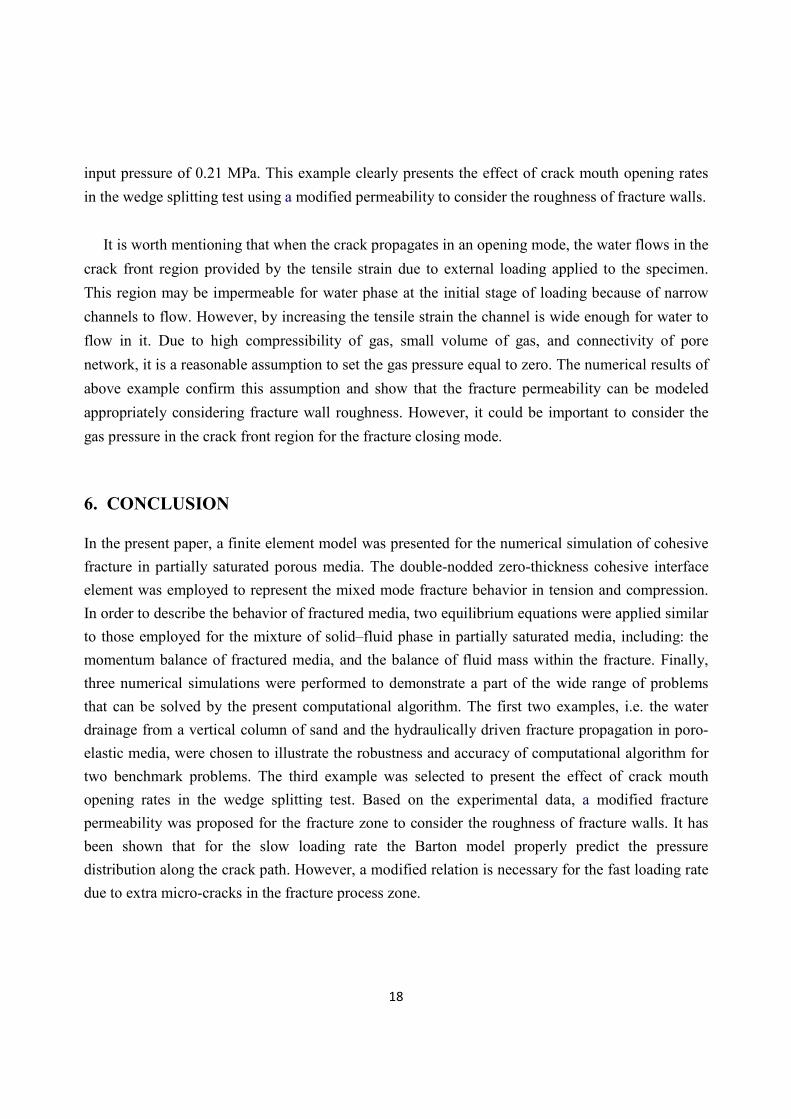
elements extensively used in literature (Khoei 2005). The relative displacements at any points along
the fracture element, as shown in Figure 2, are given by top bot= −u uδδδδ , in which , T
s nδ δ=δδδδ and
, T
s nu u=u with top)( su and top)( nu denoting the displacements in the local s and n directions of
the top side of element, and bot)( su and bot)( nu the displacements in the local s and n directions of
the bottom side of element, respectively. The relative displacements at any point of the element can
be related to the nodal values by f= N uδδδδ , with bot top( ) , ( )f f f= − N N N and
bot top , T
=u u u . In this
relation, fN is the shape functions of cohesive fracture element defined by bot 1 2( ) , f f f=N N N and
top 3 4( ) , f f f=N N N . The shear and normal strains, i.e. , nγ ε=ε , can be obtained from the
relative displacements as 1
swγ δ= and
1n nwε δ= . Hence, the strain vector can be defined as
f=ε B u , where the fB matrix is equal to 1
fwN .
In relations (20) and (21), [1, 0, 1]T
f =m and f∇N is defined as
1 2 3 4
1 2 3 4
f f f f
f
f f f f
N N N N
s s s s
N N N N
w w w w
∂ ∂ ∂ ∂ ∂ ∂ ∂ ∂ ∇ = − −
N (22)
and fk is the fracture permeability matrix defined as
=
n
l
fk
k
0
0k (23)

12
where lk is the longitudinal transverse permeability coefficient, nk is the transverse permeability
coefficient, and the relative permeability of fracture is assumed to be 1=rfk (Meschke and
Grasberger 2003).
4.1. Fracture Permeability Coefficient
In order to model the fluid flow through the discontinuity, the zero-thickness elements have been
widely used in literature, which can be classified into the single, double and triple-nodded elements.
The single-nodded elements are the simplest one, which are superimposed onto the standard
continuum mesh. The triple-nodded elements are used to model the influence of a transversal
conductivity through the discontinuity appropriately (Guiducci et al. 2002). In these elements, the
two nodes of adjacent continuum elements represent the potentials in the pore system on each side
of the interface, and the third node in the middle represents the average potential of fluid in the
channel represented by the discontinuity. However, the double-nodded interface elements have the
advantage of making it possible to use similar FE mesh for both mechanical and fluid flow analyses
(Segura and Carol 2004). In the case that the influence of a transversal conductivity is not
considered, these elements are similar to the single nodded type although they are geometrically
double-nodded, and when the time comes to solve the system, the two nodes must have the same
potential. This limitation may, however, be avoided by assuming that the potential in the channel is
the average of two sides of the interface. Based on this simple assumption, an alternative flow
interface model has been recently developed by Khoei et al. (2009b), which preserves both
longitudinal and transversal conductivities.
The existence of fracture besides the longitudinal conductivity may also represent an obstacle for
fluid flow in the transversal direction because of the potential drop due to the transition from a pore
system into an open channel and back into a pore system. Thus, defining the flow potential Φ equal
to zbup w )( −+ &&ρ , with z denoting the distance from a datum, a jump is admitted in the total flow
potential field across the fracture related to transverse fluid flux tq travelling normal to the
discontinuity. Considering a discrete version of the Darcy law, in which the total flow potential drop
plays the role of total flow potential gradient, the transverse fluid flux is linked to the difference of
hydraulic potentials between the two surfaces defining the discontinuity by )( +− Φ−Φ= tt kq ,
where tk is a transverse hydraulic permeability coefficient and the superscripts – and + stand for
each side of the discontinuity (Segura and Carol 2004). In fact, it can be concluded that the single-
13
nodded interfaces are equivalent to the double-nodded and triple-nodded elements with ∞=tk , i.e.
the infinite transversal conductivity.
It is desirable to implement the inactive cohesive interface elements in both mechanical and fluid
flow media before the critical stress is reached. In fact, an infinite initial stiffness provides a rigid
inactive element for mechanical part before the maximum tensile stress is reached. Also, assuming
an infinite transversal conductivity and zero longitudinal conductivity lead to inactive elements for
flow part before stress reaches the tensile strength of media. Comparing the transverse permeability
coefficient nk with the permeability coefficient tk introduced by Segura and Carol (2004), it can be
concluded that wkk nt = , which leads to inactive cohesive elements for fluid flow before stress
reaches the tensile strength of material at that point. However, in order to avoid the numerical
difficulty, when aperture is zero an initial large value of tk is assumed instead of wkn .
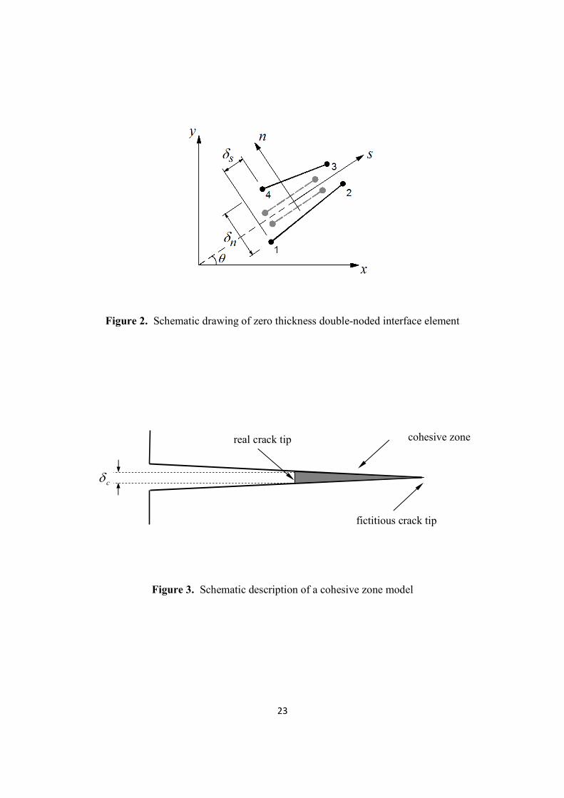
In order to model the longitudinal transverse permeability, the fractured zone is decomposed into
two portions; one is related to the cohesive area and the other is related to the real cracked zone
where the cohesive forces are zero (Figure 3), in which the permeability of real cracked zone is
identical to the natural fracture. One of the simplest techniques to model the flow through a natural
fracture is based on the parallel plate model. This is the only fracture model for which an exact
calculation of the hydraulic conductivity is possible; this calculation yields the well-known 'cubic
law' (Witherspoon et al. 1980). The derivation of the cubic law begins by assuming that the fracture
walls can be represented by two smooth, parallel plates with infinite dimensions, separated by an
aperture w. However, the real fractures have finite sizes, rough walls and variable apertures. It was
shown that the parallel plate model is inadequate to describe the flow in natural fractures (Sisavath
et al. 2003).
For a natural fracture, the aperture can generally be defined as mechanical (geometrically
measured), or hydraulic (measured by analysis of the fluid flow). The mechanical joint aperture w is
defined as the average point-to-point distance between two points of surfaces, perpendicular to the
selected plane. The hydraulic aperture e can be determined from laboratory fluid-flow experiments.
An important distinction has to be made between the theoretical smooth wall hydraulic aperture e
and the real mechanical aperture w (geometrically measured) between two irregular joint walls.
Owing to the wall friction and the tortuosity, w is generally larger than e. An empirical model was
proposed by Barton et al. (1985) relating the hydraulic aperture e to the real mechanical aperture w
and the joint roughness JRC . This relationship was defined based on the experimental data as

14
2
2.5
we
JRC= (24)
where e and w are expressed in micro-metres. It must be noted that this equation is only valid for
ew ≥ . The roughness of the crack surface depends on the toughness and size of aggregates and the
properties of matrix and interface. It is assumed that the hydraulic aperture for cohesive zone is a
function of w which is zero at the fictitious crack tip and equal to 5.22 JRCcδ at real crack tip. This
function can be defined via the experimental data. Based on the hydraulic aperture in the fractured
zone, the longitudinal transverse permeability coefficient lk can be expressed as
2 12e µ , with µ
denoting the dynamic viscosity.
5. NUMERICAL SIMULATION RESULTS
In order to demonstrate a part of the wide range of problems that can be solved by the present
approach, we have illustrated the performance of proposed computational algorithm in modeling of
fracture propagation in partially saturated porous media. The finite element model is applied in
partially saturated porous media and the cohesive interface elements are employed in the fractured
zone where the cohesive tractions develop. The implementation of cohesive fracture elements is
illustrated due to fluid flow inside the crack and the values of crack mouth opening are obtained as
the crack proceeds. The first two examples are selected to illustrate the robustness and accuracy of
computational algorithm for two benchmark problems. The first example deals with the drainage of
water from a vertical column of sand to present the accuracy of proposed computational algorithm
against the experimental results conducted by Liakopoulos (1965). The second example illustrates
the performance of cohesive fracture elements for the simulation of hydraulically driven fracture
propagation in poroelastic media against an analytical solution by Spence and Sharp (1985) and its
numerical evaluation by Boone and Ingraffea (1990). Finally, the last example is chosen to
demonstrate the capability of proposed model for the wedge splitting test performed by Slowik and
Saouma (2000) at different rates of crack mouth opening.
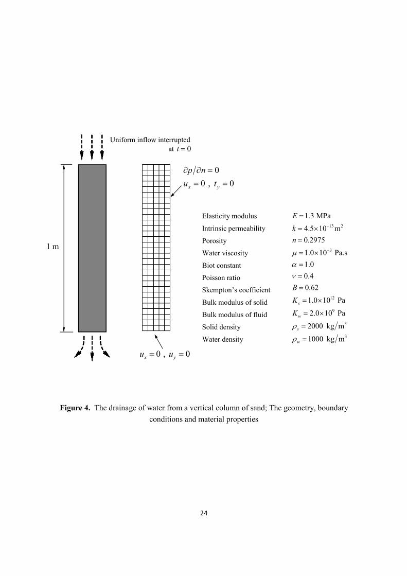
5.1. Water Drainage from a Column of Sand
The first example is chosen to evaluate the accuracy of computational modeling for the drainage of
water from a vertical column of sand with those experimentally obtained by Liakopoulos (1965) and
15
numerically reported by Lewis and Schrefler (1998). The problem was considered by various
researchers to verify their numerical analysis, and referred as a representative of wide range of
problems involving gravity-governed partially saturated porous media since no external loads are
applied. A perspex column of 1 m high is packed with sand and instrumented with tension-meters to
measure the moisture tension at various points within the column. In order to apply the initial
boundary conditions of laboratory test, water is added continuously from the top of column and is
allowed to drain freely at the bottom through a filter, as shown in Figure 4. The flow is carefully
regulated until the tension-meters read zero pore pressure. At this stage, the inflow of water from
the top is stopped and the upper boundary is made impermeable to water as an initial boundary
conditions. From then the tension-meter readings are recorded. The assumed material properties of
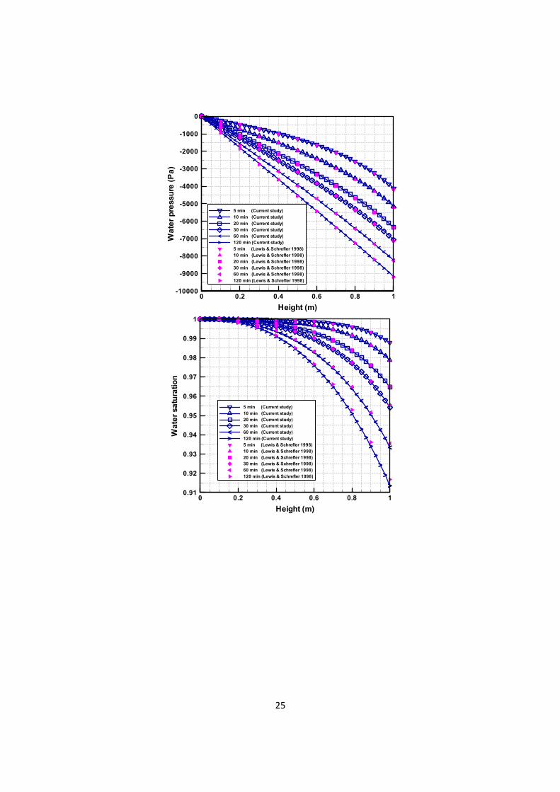
sand together with the geometry and boundary conditions of the problem are shown in Figure 4. In
Figure 5, the numerical results of partially saturated model for the water pressure, water saturation,
and vertical displacement distribution versus the column height are presented for different times of
5, 10, 20, 30, 60 and 120 min. Clearly, it can be seen that the numerical results are in complete
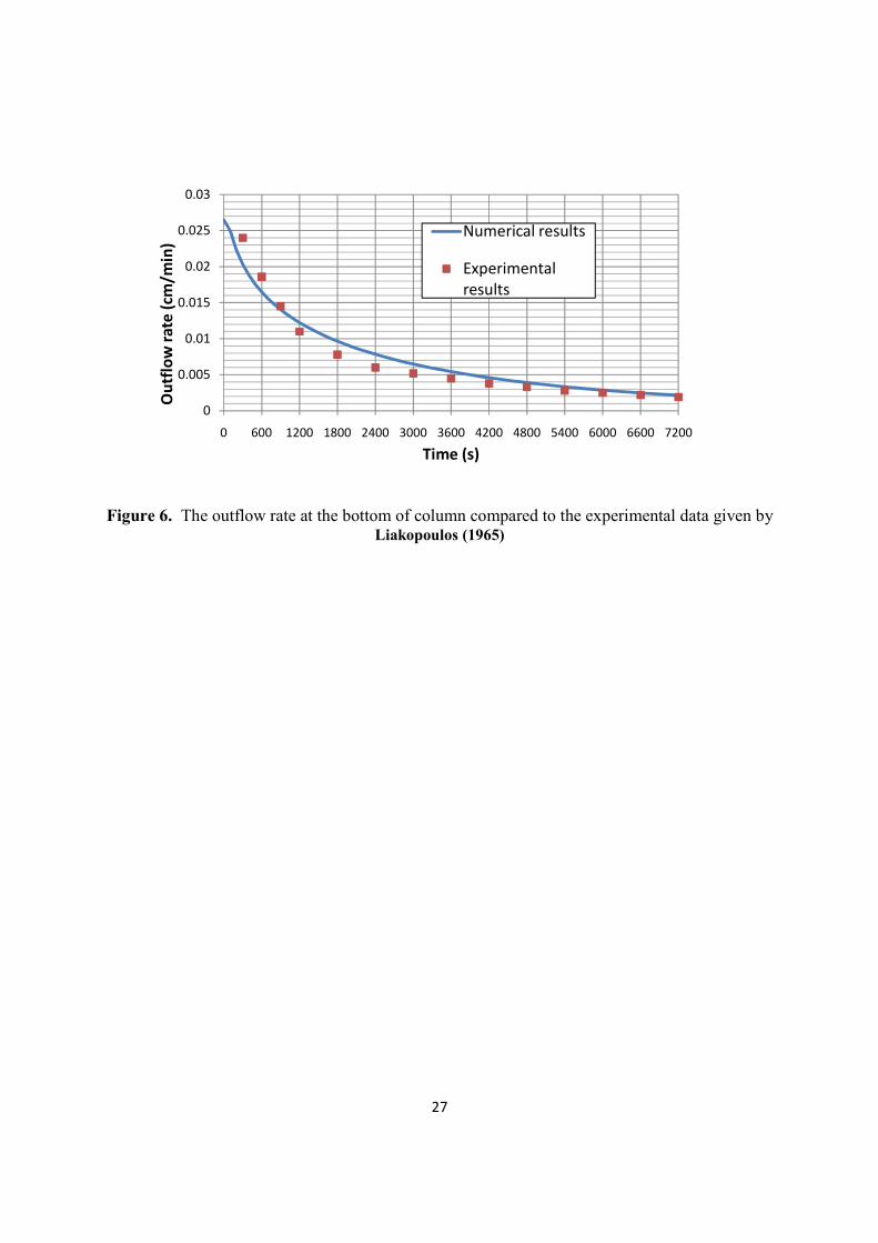
agreement with those reported by Lewis and Schrefler (1998). Figure 6 presents the time history of
outflow rate at the base of column. Obviously, the outflow rate gradually decreases to zero with
time after stopping the inflow of water from the top at time 0t = . The curve shows a good
agreement between the numerical result and experimental data given by Liakopoulos (1965).
5.2. Hydraulic Fracturing
The second example illustrates the performance of cohesive fracture elements for the simulation of
hydraulically driven fracture propagation in poroelastic media. This example is chosen here since
the leakage flux into the surrounding porous media across the fracture border is important in
hydraulic fracture modeling. An analytical solution was obtained for this example by Spence and
Sharp (1985) and the numerical simulation by Boone and Ingraffea (1990), in which a finite element
method was applied for the mechanical problem and a finite difference method for the flow analysis
through the fracture. In Figure 7, the geometry, boundary condition and finite element mesh of
problem are presented together with the material properties. An initial crack is assumed at the
borehole where the crack propagates, and a constant flow rate of 30.0001 m /s is applied at the crack
mouth. The crack propagates when the principle effective stress at crack tip reaches the ultimate
tensile strength of the material assumed to be 0.5 MPa.

16
The length of cohesive elements is chosen so that the fracture process zone is discretized with
adequate resolution and the need for numerical convergence is satisfied. The length of process zone
cR can be approximated by 2
c f tR E G fη ′ ′= (Bazant and Planas 1998), where fG is the specific
fracture energy, tf ′ the tensile strength, η a constant equal to 8π according to Barenblatt cohesive
theory, and E′ the effective elastic modulus defined as E for plane stress and )1/( 2υ−E for plane
strain problems. The limiting values for the size of a fully developed fracture process zone range
from 0.3 m to 2 m for concrete and similar quasi-brittle materials. For a brittle material, it is
generally argued that 2–5 elements are necessary to resolve the cohesive zone (Zhou et al. 2005). By
evaluating the process zone length and determining the cohesive elements length, a uniform mesh is
generated in the area surrounding the crack. The mesh uniformity is ascertained by local remeshing
in this area. In addition, a rosette configuration with uniform elements around crack tip is
constructed by adding new boundaries around the crack tip. The random orientation of elements is
gained by using a Delaunay based unstructured grid generator (Khoei et al. 2008). It is assumed that
the crack propagation takes place according to Dugdale (1960) and Barrenblatt (1962) cohesive
models, in which the traction principle effective stress at crack tip reaches the ultimate tensile
strength of the material.
Figure 8 presents the variations with time of the crack length, crack mouth opening (CMOD),
and pressure distribution along crack mouth. The results of numerical simulations are compared
with those reported by Spence and Sharp (1985). A good agreement can be observed between two
different simulations. In Figure 9, the distribution of maximum principal effective stress contours
are presented at 2.0, 4.0, 6.0t = and 9 s .
5.3. The Wedge Splitting Test
The last example demonstrates the capability of proposed computational model for the wedge
splitting test performed experimentally by Slowik and Saouma (2000). The geometry and boundary
conditions of specimen are shown in Figure 10. The water input pressure is applied only at notch
section while zero pressure is assumed at the rest of boundary. Two different rates are used for the
crack mouth opening displacement (CMOD), including the slow crack opening with the rate of
2 m sµ and the fast crack opening with the rate of 200 m sµ . It is well known that the higher

17
velocity of crack mouth opening may develop extra micro-cracks within the crack tip zone since
they have no time to unload each other. As a result, due to fast growth of the main crack, several
micro-cracks may be formed at the main crack tip zone that dissipates more energy. Although the
multi-microcracking process in the fast crack growth may result in the increase of local stress, this
stress increase is less important compared to the increase of fracture energy. It was assumed by
Bazant and Li (1997a, b) that the normalized effective stress – displacement ( )c cσ δ− curve expands
outwards when the cohesive opening rate increases. It was also shown by Zhou and Molinari (2004)
that the failure strength of ceramic increases by 10–15% when the strain rate increases 125 times.
Hence, it can be concluded that both cσ and cδ increase with the increase of crack velocity.
The material properties employed for experimental tests in the case of fast and slow loading rates
are given in Table 1. It has been observed from numerical simulations that the increase of micro-
cracks due to fast loading rate increases the permeability of fracture process zone. It is obtained that
in the slow loading rate, the Barton model with JRC equal to 20 satisfactorily predicts the
hydraulic aperture for the entire of fracture, however – using this relation for the fast loading rate
leads to the lower pressure through the fracture path in comparison with the experimental data. It is
also observed that a linear function between the hydraulic and mechanical apertures improves the
results effectively in the fracture process zone although the quadratic function was proposed by
Barton et al. (1985).
In Figure 11, the variations of applied force with crack mouth opening displacement (CMOD)
are plotted for both experimental and numerical results of the wedge splitting test in the case of
slow and fast loading rates at the water input pressure of 0.21 MPa. Figure 12 presents the
experimentally and numerically variations of pressure distributions along the crack path for
different time steps in the case of slow loading rate at the water input pressure of 0.21 MPa. Also
plotted in Figure 13 are the variations of pressure distributions along the crack path for the fast
loading rate. In Figure 14, the experimental and numerical results of pressure distributions are
depicted for various time steps in the case of fast loading rate at the water input pressure of 0.62
MPa. Obviously, good agreements can be seen between the experimental and numerical results. The
results indicate that the proposed permeability properly predict the fluid flow through the fracture
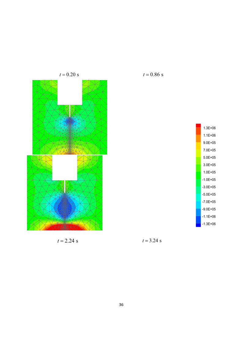
zone. In Figure 15, the distribution of effective stress xσ ′ contours are shown at time steps 2.0=t ,
0.86 , 2.24 and 3.24 s for the fast loading rate at the water input pressure of 0.21 MPa. Finally, the
variations of normal cohesive traction along the fracture length are plotted in Figure 16 at the water
18
input pressure of 0.21 MPa. This example clearly presents the effect of crack mouth opening rates
in the wedge splitting test using a modified permeability to consider the roughness of fracture walls.
It is worth mentioning that when the crack propagates in an opening mode, the water flows in the
crack front region provided by the tensile strain due to external loading applied to the specimen.
This region may be impermeable for water phase at the initial stage of loading because of narrow
channels to flow. However, by increasing the tensile strain the channel is wide enough for water to
flow in it. Due to high compressibility of gas, small volume of gas, and connectivity of pore
network, it is a reasonable assumption to set the gas pressure equal to zero. The numerical results of
above example confirm this assumption and show that the fracture permeability can be modeled
appropriately considering fracture wall roughness. However, it could be important to consider the
gas pressure in the crack front region for the fracture closing mode.
6. CONCLUSION
In the present paper, a finite element model was presented for the numerical simulation of cohesive
fracture in partially saturated porous media. The double-nodded zero-thickness cohesive interface
element was employed to represent the mixed mode fracture behavior in tension and compression.
In order to describe the behavior of fractured media, two equilibrium equations were applied similar
to those employed for the mixture of solid–fluid phase in partially saturated media, including: the
momentum balance of fractured media, and the balance of fluid mass within the fracture. Finally,
three numerical simulations were performed to demonstrate a part of the wide range of problems
that can be solved by the present computational algorithm. The first two examples, i.e. the water
drainage from a vertical column of sand and the hydraulically driven fracture propagation in poro-
elastic media, were chosen to illustrate the robustness and accuracy of computational algorithm for
two benchmark problems. The third example was selected to present the effect of crack mouth
opening rates in the wedge splitting test. Based on the experimental data, a modified fracture
permeability was proposed for the fracture zone to consider the roughness of fracture walls. It has
been shown that for the slow loading rate the Barton model properly predict the pressure
distribution along the crack path. However, a modified relation is necessary for the fast loading rate
due to extra micro-cracks in the fracture process zone.

19
REFERENCES
Alonso EE, Gens A, Josa A (1990) A constitutive model for partially saturated soils. Geotech 40: 405–430.
Barenblatt GI (1962) The mathematical theory of equilibrium cracks in brittle fracture. Adv Appl Mech 7:
55–62.
Baroghel-Bouny V, Mainguy M, Lassabatere T, Coussy O (1999) Characterization and identification of
equilibrium and transfer moisture properties for ordinary and high-performance cementitious materials.
Cem Conc Res 29: 1225–1238.
Barton N, Bandis S, Bakhtar K (1985) Strength, deformation and conductivity coupling of rock joints. Int J
Rock Mech Min Sci Geomech Abstr 22: 121–140.
Bazant ZP, Li YN (1997a) Cohesive crack with rate-dependent opening and viscoelasticity: 1. Mathematical
model and scaling. Int. J. Fract 86: 247–265.
Bazant ZP, Li YN (1997b) Cohesive crack with rate-dependent opening and viscoelasticity: 2. Numerical
algorithm, behavior and size effect. Int. J. Fract 86: 267–288.
Bazant ZP, Planas J (1998) Fracture and Size Effect in Concrete and Other Quasibrittle Materials. CRC
Press, New York, USA
Biot MA (1941) General theory of three dimensional consolidation. J Appl Phys 12: 155–164.
Birgisson B, Montepara A, Romeo E, Roncella R, Napier JAL, Tebaldi G (2008) Determination and
prediction of crack patterns in hot mix asphalt (HMA) mixtures. Eng Frac Mech 75: 664–673.
Boone TJ, Ingraffea AR (1990) A numerical procedure for simulation of hydraulically driven fracture
propagation in poroelastic media. Int J Numer Analy Meth Geomech 14: 27–47.
Brühwiler E, Saoma VE (1995a) Water fracture interaction in concrete. Part I: Fracture properties. ACI
Mater J 92: 296–303.
Brühwiler E, Saoma VE (1995b) Water fracture interaction in concrete. Part II: Hydrostatic pressure in
cracks. ACI Mater J 92: 383–390.
Camacho GT, Ortiz M (1996) Computational modeling of impact damage in brittle materials. Int J Solids
Struct 33: 2899–2938.
Dugdale DS (1960) Yielding of steel sheets containing slits. J Mech Phys Solids 8: 100–108.
Gawin D, Schrefler BA (1996) Thermo-hydro-mechanical analysis of partially saturated porous materials.
Eng Comput 13: 113–143.
Ghaboussi J, Wilson EL (1973) Flow of compressible fluid in porous elastic media. Int J Numer Methods
Eng 5: 419–442.
Guiducci C, Pellegrino A, Radu JP, Collin F, Charlier R (2002) Numerical modeling of hydro-mechanical
fracture behavior. In Numerical Models in Geomechanics- NUMOG VIII, Pande GN, Pietruszczak S (Eds).
Swets & Zeitlinger, 293–299.

20
Hilleborg A, Modeer M, Petersson PE (1976) Analysis of crack formation and crack growth in concrete by
means of fracture mechanics and finite elements. Cem Conc Res 6: 773–782.
Jenq Y, Shah SP (1991) Features of mechanics of quasi-brittle crack propagation in concrete, Int J Fract 51:
103–120.
Khoei AR (2005) Computational Plasticity in Powder Forming Processes. Elsevier, UK.
Khoei AR, Azadi H, Moslemi H (2008) Modeling of crack propagation via an automatic adaptive mesh
refinement based on modified superconvergent patch recovery technique. Engng Fract Mech 75: 2921–
2945.
Khoei AR, Azami AR, Haeri SM (2004) Implementation of plasticity based models in dynamic analysis of
earth and rockfill dams: A comparison of Pastor-Zienkiewicz and cap models. Comput Geotech. 31: 385–
410.
Khoei AR, Barani OR, Mofid M (2009a) Modeling of dynamic cohesive fracture propagation in porous
saturated media. Submitted to: Int J Numer Anal Methods Geomech.
Khoei AR, Gharehbaghi SA, Azami AR, Tabarraie AR (2006) SUT-DAM: An integrated software
environment for multi-disciplinary geotechnical engineering. Advan Eng Software 37: 728–753.
Khoei AR, Moslemi H, Majd Ardakany K, Barani OR, Azadi H (2009b) Modeling of cohesive crack growth
using an adaptive mesh refinement via the modified–SPR technique, Int J Fracture 159: 21–41.
Lewis RW, Schrefler BA (1998) The Finite Element Method in the Static and Dynamic Deformation and
Consolidation of Porous Media. John Wiley, New York.
Liakopoulos AC (1965) Transient flow through unsaturated porous media, PhD thesis, University of
California, Berkeley, CA.
Meschke G, Grasberger S (2003) Numerical modeling of coupled hygromechanical degradation of
cementitious materials. J Eng Mech 129: 383–392.
Ortiz M, Suresh S (1993) Statistical properties of residual stresses and intergranular fracture in ceramic
materials. J Appl Mech 60: 77–84.
Persson B (1997) Moisture in concrete subjected to different kinds of curing. Mater Struct 30: 533–544.
Reinhardt HW, Sosoro M, Zhu X (1998) Cracked and repaired concrete subject to fluid penetration. Mat
Struct 31, 74–93.
Rescher OJ (1990) Importance of cracking in concrete dams. Engng Fract Mech 35: 503–524.
Savage BM, Janssen DJ (1997) Soil physics principles validated for use in predicting unsaturated moisture
movement in portland cement concrete. ACI Mater J 94: 63–70.
Schrefler BA, Secchi S, Simoni L (2006) On adaptive refinement techniques in multi-field problems
including cohesive fracture. Comput Methods Appl Mech Eng 195: 444–461.
Secchi S, Simoni L, Schrefler BA (2007) Mesh adaptation and transfer schemes for discrete fracture
propagation in porous materials. Int J Numer Anal Methods Geomech 31: 331–345.

21
Segura JM, Carol I (2004) On zero-thickness elements for diffusion problems. Int J Numer Anal Methods in
Geomech 28: 947–962.
Shum, KM, Hutchinson JW (1990) On Toughening by Micro-Cracks. Mech Mat 9: 83–91.
Simoni L, Secchi S (2003) Cohesive fracture mechanics for a multi-phase porous medium. Eng Comput 20:
675–698.
Sisavath S, Al-Yaarubi A, Pain C, Zimmerman RW (2003) A simple model for deviation from the cubic law
for a fracture undergoing dilation or closure. Pure Appl Geophys 160: 1009–1022.
Slowik V, Saouma VE (2000) Water pressure in propagating concrete cracks. J Struct Eng ASCE 126: 235–
242.
Song SH, Paulino GP, Buttlar WG (2006) A bilinear cohesive zone model tailored for fracture of asphalt
concrete considering viscoelastic bulk material. Eng Fract Mech 73: 2829–2848.
Spence DA, Sharp P (1985) Self-similar solutions for elasto-hydrodynamic cavity flow. Proc Royal Soc
London A 400: 289–313.
van Genuchten M (1980) A closed-form equation for predicting the hydraulic conductivity of unsaturated
soil. Soil Sci Soc Am J. 44: 892– 898.
Witherspoon PA, Wang JSY, Iwai K, Gale JE (1980) Validity of cubic low for fluid flow in a deformable
rock fracture. Water Resour Res 16: 1016–1024.
Xu XP, Needleman A (1994) Numerical simulations of fast crack growth in brittle solids. J Mech Phys
Solids 42: 1397–1434.
Zhou F, Molinari JF, Shioya T (2005) A rate-dependent cohesive model for simulating dynamic crack
propagation in brittle materials. Eng Fract Mech 72: 1383–1410.
Zhou F, Molinari JF (2004) Stochastic fracture of ceramics under dynamic tensile loading. Int. J. Solids
Struct 41: 6573–6596.
Zhu X, Pekau OA (2007) Seismic behavior of concrete gravity dams with penetrated cracks and equivalent
impact damping. Engrg Struct 29: 336–345.
Zienkiewicz OC, Chan AHC, Pastor M, Schrefler BA, Shiomi T (1999) Computational Geomechanics with
Special Reference to Earthquake Engineering. Wiley.

22
Figure 1. A bilinear cohesive law in terms of normalized effective displacement and normalized
effective traction
eδ
et
crλ
0 1
1
Normalized effective displacement
Norm
aliz
ed e
ffec
tive
trac
tion
et
eδ
23
Figure 2. Schematic drawing of zero thickness double-noded interface element
Figure 3. Schematic description of a cohesive zone model
cδ
real crack tip cohesive zone
fictitious crack tip
24
Figure 4. The drainage of water from a vertical column of sand; The geometry, boundary
conditions and material properties
Elasticity modulus
Intrinsic permeability
Porosity
Water viscosity
Biot constant
Poisson ratio
Skempton’s coefficient
Bulk modulus of solid
Bulk modulus of fluid
Solid density
Water density
13 2
3
12
9
3
3
1.3 MPa
4.5 10 m
0.2975
1.0 10 Pa.s
1.0
0.4
0.62
1.0 10 Pa
2.0 10 Pa
2000 kg m
1000 kg m
s
w
s
w
E
k
n
B
K
K
µαν
ρ
ρ
−
−
=
= ×
=
= ×
=
=
=
= ×
= ×
=
=
0 , 0x yu u= =
Uniform inflow interrupted
at 0t =
0
0 , 0x y
p n
u t
∂ ∂ =
= =
1 m
25
<<<<<<<<<<<<<<<<<<<<<<<<<<<<<<<<<<<<<<<<<<<<<<<<<<<<<<<<<<<<<<<<<<<<<<<<<<<<<<<<<<
>>>>>>>>>>>>>>>>>>>>>>>>>>>>>>>>>>>>>>>>>>>>>>>>>>>>>>>>>>>>>>>>>>>>>>>>>>>>>>>>>>
Height (m)
Waterpressure(Pa)
0 0.2 0.4 0.6 0.8 1-10000
-9000
-8000
-7000
-6000
-5000
-4000
-3000
-2000
-1000
0
5 min (Current study)
10 min (Current study)
20 min (Current study)
30 min (Current study)
60 min (Current study)
120 min (Current study)
5 min (Lewis & Schrefler 1998)
10 min (Lewis & Schrefler 1998)
20 min (Lewis & Schrefler 1998)
30 min (Lewis & Schrefler 1998)
60 min (Lewis & Schrefler 1998)
120 min (Lewis & Schrefler 1998)
<>
<<<<<<<<<<<<<<<<<<<<<<<<<<<<<<<<<<<<<<<<<<<<<<<<<<<<<<<<<<<<<<<<<<<<<<<<<<<<<<<<
<<
>>>>>>>>>>>>>>>>>>>>>>>>>>>>>>>>>>>>>>>>>>>>>>>>>>>>>>>>>>>>>>>>>>>>>>>>>>
>>
>>
>>
>>
Height (m)
Watersaturation
0 0.2 0.4 0.6 0.8 10.91
0.92
0.93
0.94
0.95
0.96
0.97
0.98
0.99
1
5 min (Current study)
10 min (Current study)
20 min (Current study)
30 min (Current study)
60 min (Current study)
120 min (Current study)
5 min (Lewis & Schrefler 1998)
10 min (Lewis & Schrefler 1998)
20 min (Lewis & Schrefler 1998)
30 min (Lewis & Schrefler 1998)
60 min (Lewis & Schrefler 1998)
120 min (Lewis & Schrefler 1998)
<>

26
Figure 5. Comparison of the numerical simulation results obtained by the present study and those
reported by Lewis and Schrefler (1998) for water drainage from a vertical column of sand;
variations of the water pressure (Pa), water saturation, and vertical displacement (m) versus column
height
<<<<<<<<<<<<<<<<<<<<<<<<<<<<<<<<<<<<<<<<<<<<<<<<<<<<<<<<<<<<<<<<<<<<<<<<<<<<<<<<<<
>>>>>>>>>>>>>>>>>>>>>>>>>>>>>>>>>>>>>>>>>>>>>>>>>>>>>>>>>>>>>>>>>>>>>>>>>>>>>>>>>>
Height (m)
Verticaldisplacement(m)
0 0.2 0.4 0.6 0.8 1
-0.0014
-0.0012
-0.0010
-0.0008
-0.0006
-0.0004
-0.0002
0.0000
5 min (Current study)
10 min (Current study)
20 min (Current study)
30 min (Current study)
60 min (Current study)
120 min (Current study)
5 min (Lewis & Schrefler 1998)
10 min (Lewis & Schrefler 1998)
20 min (Lewis & Schrefler 1998)
30 min (Lewis & Schrefler 1998)
60 min (Lewis & Schrefler 1998)
120 min (Lewis & Schrefler 1998)
<>
27
Figure 6. The outflow rate at the bottom of column compared to the experimental data given by Liakopoulos (1965)
0
0.005
0.01
0.015
0.02
0.025
0.03
0 600 1200 1800 2400 3000 3600 4200 4800 5400 6000 6600 7200
Ou
tflo
w r
ate
(cm
/min
)
Time (s)
Numerical results
Experimental
results

28
Figure 7. The hydraulic fracture problem; The geometry and boundary conditions
p = 0
80
10
160
u x = , u y = 0
u y = 0 0=yu
0 , 0 , 0x yp u u= = =
Elasticity modulus
Permeability coefficient
Shear modulus
Undrained Poisson ratio
Drained Poisson ratio
Skempton coefficient
Bulk modulus of solid
Bulk modulus of fluid
Porosity
Fluid viscosity
Biot coefficient
6 2
9
15960 MPa
6 10 m (MPa .s)
6000 MPa
0.33
0.20
0.62
36000 MPa
3000 MPa
0.19
10 MPa.s
0.79
u
s
f
E
k
G
B
K
K
n
ν
ν
µα
−
−
=
= ×
=
=
=
=
=
=
=
=
=

29
Figure 8. The variations with time of the crack length, crack mouth opening (CMOD), and
pressure distribution along crack mouth with those reported by Spence and Sharp (1985)
0
0.5
1
1.5
2
2.5
3
3.5
4
4.5
0 2 4 6 8 10
Cra
ck l
en
gth
(m
)
Time (s)
Numerical solution
Spence et. al.
solution
0
0.5
1
1.5
2
2.5
3
3.5
0 2 4 6 8 10
CM
OD
(m
m)
Time (s)
Numerical solution
Spence et. al.
solution
0
0.5
1
1.5
2
2.5
0 2 4 6 8 10
Pre
ssu
re (
MP
a)
Time (s)
Numerical solution
Spence et. al.
solution

30
Figure 9. The distribution of maximum principal effective stress contours at various time steps
2.0, 4.0, 6.0t = and 9 s
0.0E+00
-1.0E+04
-5.0E+04
-1.0E+05
-2.0E+05
-3.0E+05
-4.0E+05
-5.0E+05

31
Figure 10. The specimen geometry and boundary conditions (all dimensions in mm)
20
100 100 100
100
50
150
4

32
Figure 11. The load versus CMOD for the slow and fast loading; A comparison between the
numerical results and experimental data
0
0.5
1
1.5
2
2.5
3
3.5
0.0 0.2 0.4 0.6 0.8 1.0
P (KN)
CMOD (mm)
Slow loading (Experimental results)
Fast loading (Experimental results)
Slow loading (Numerical results)
Fast loading (Numerical results)
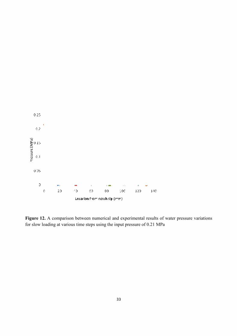
Figure 12. A comparison betwe
for slow loading at various time s
33
between numerical and experimental results of w
time steps using the input pressure of 0.21 MPa
water pressure variations

Figure 13. A comparison betwe
for fast loading at various time st
34
between numerical and experimental results of wa
ime steps using the input pressure of 0.21 MPa
water pressure variations
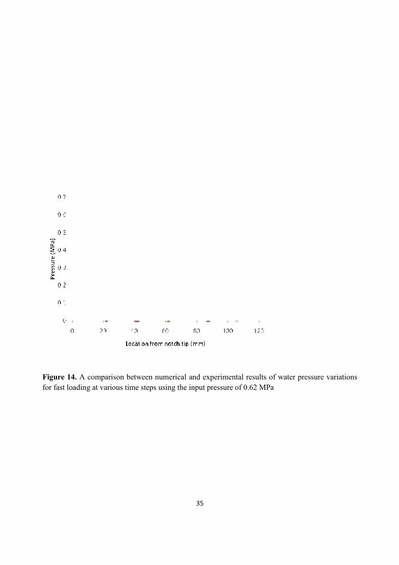
Figure 14. A comparison betwe
for fast loading at various time st
35
between numerical and experimental results of wa
ime steps using the input pressure of 0.62 MPa
water pressure variations
36
0.20 st = 0.86 st =
2.24 st = 3.24 st =
1.3E+06
1.1E+06
9.0E+05
7.0E+05
5.0E+05
3.0E+05
1.0E+05
-1.0E+05
-3.0E+05
-5.0E+05
-7.0E+05
-9.0E+05
-1.1E+06
-1.3E+06

37
Figure 15. The distribution of effective stress xσ ′ contours at various time steps for fast loading
using the input pressure of 0.21 MPa (all dimensions in Pa), Compression assumed to be positive.

Figure 16. The variations of n
steps for the input pressure of 0.2
38
of normal cohesive traction along the fracture
of 0.21 MPa
cture length at various time
39
Table 1. The material parameters for concrete
Material properties Fast loading Slow loading
Elasticity modulus (MPa) 25000 25000
Poisson ratio 0.17 0.17
Density of solid particles ( 3kg/m ) 2720 2720
Water density ( 3kg/m ) 1000 1000
Tensile strength (MPa) 1.32 1.25
Critical displacement cδ ( mm) 0.25 0.2
Permeability ( 2m Pa s ) 1510− 1510−
Prosity 0.1 0.1
Bulk modulus of solid (MPa) 36000 36000
Bulk modulus of fluid (MPa) 3000 3000
Fluid viscosity (MPa s) 910− 910−


![Thermal Conductivity of Saturated Samples Using the Hot ...wseas.us/e-library/conferences/2006elounda2/papers/538-180.pdf · partially saturated samples, see for example, Middleton[3].](https://static.fdocuments.net/doc/165x107/5faff89875f1183acf62e59f/thermal-conductivity-of-saturated-samples-using-the-hot-wseasuse-libraryconferences2006elounda2papers538-180pdf.jpg)


