Fuel Processing Technology, 29 (1991) 1-17 1 Elsevier Science Publishers B.V., Amsterdam

Modeling of a hydrocracking reactor

S. Mohanty*, D.N. Saraf and D. Kunzru**

Department of Chemical Engineering, Indian Institute of Technology, Kanpur-208 016 (India)

(Received June 5th, 1990; accepted in revised form April 1 lth, 1991 )

Abstract

A three parameter model has been developed for a two-stage vacuum gas oil hydrocracker unit. The feed and the products were lumped into 23 pseudocomponents, each characterized by its boiling range and specific gravity. The model assumes that each pseudocomponent can only form lighter products by a pseudohomogeneous first order reaction. The model parameters were deter- mined using information from literature and plant data. Given the feed characterization and the inlet conditions, the concentration and temperature profiles throughout the reactors, the amount of recycle and hydrogen consumption can be calculated. The model was validated against plant data and the agreement was generally good. The effect of variation in the model parameters and operating conditions has also been discussed.

INTRODUCTION

The rapid increase in the demand for diesel-kerosene fractions has resulted in the development of many new processes which can convert the heavier pe- troleum fractions into more usable lighter products. The availability of large quantities of cheap by-product hydrogen from catalytic reforming has made the hydrogenation processes quite attractive. Hydrocracking is one of the ear- liest applications of hydrogenation and is of current interest because it is ex- tremely versatile for processing a variety of difficult-to-use feedstocks into a wide spectrum of desirable products. Although several kinetic studies and types of catalyst used for hydrocracking of pure hydrocarbons and petroleum frac- tions are available in the literature, very little information on reactor modeling has been published [ 1-5 ].

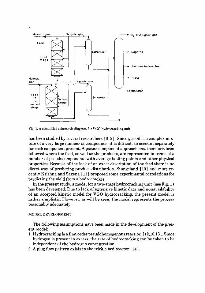
Three-phase reactors (gas-solid-liquid) of trickle-bed type are widely used for hydrocracking of vacuum gas oil (VGO). A two-reactor design with recycle is commonly used for hydrocracking plants, a simplified schematic diagram for which is shown in Fig. 1. Hydrocracking of n-alkanes over different catalysts

*Presently at Regional Research Laboratory, Bhutneswar. **To whom correspondence should be addressed.

0378-3820/91/$03.50 © 1991 Elsevier Science Publishers B.V. All rights reserved

Makeup gas Recycle gas

First ~ ~l:~rator stage

Makeup Recycle gas

g a s , f f

Feed ~ S c c o n d 11 to ~ Sep~:lrator

the seconc L,,j ~ . j stage stage l j ~

=' C 4 and tighter gas

b Naphtha

Aviation turbine fuel

D Diesel

Fractionator

Fig. 1. A simplified schematic diagram for VGO hydrocracking unit.

has been studied by several researchers [ 6-9 ]. Since gas oil is a complex mix- ture of a very large number of compounds, it is difficult to account separately for each component present. A pseudocomponent approach has, therefore, been followed where the feed, as well as the products, are represented in terms of a number of pseudocomponents with average boiling points and other physical properties. Because of the lack of an exact description of the feed there is no direct way of predicting product distribution. Stangeland [ 10] and more re- cently Krishna and Saxena [ 11 ] proposed some experimental correlations for predicting the yield from a hydrocracker.

In the present study, a model for a two-stage hydrocracking unit (see Fig. 1 ) has been developed. Due to lack of extensive kinetic data and nonavailability of an accepted kinetic model for VGO hydrocracking, the present model is rather simplistic. However, as will be seen, the model represents the process reasonably adequately.

MODEL DEVELOPMENT

The following assumptions have been made in the development of the pres- ent model: 1. Hydrocracking is a first order pseudohomogenous reaction [ 12,10,13 ]. Since

hydrogen is present in excess, the rate of hydrocracking can be taken to be independent of the hydrogen concentration.

2. A plug flow pat tern exists in the trickle bed reactor [ 14 ].

3. Heat losses are negligible and the commercial reactors operate under adi- abatic conditions [ 14 ].

4. Diffusional resistances are absent [15,2]. 5. It is steady state operation. 6. Recycle and make-up gases are pure hydrogen. 7. The petroleum feed and the products are in the liquid phase in the reactor. 8. The summation of the product of the total mass flow rate and its heat ca-

pacity is constant for each catalyst bed. The concept of pseudocomponents has been incorporated to divide the wide

boiling range VGO into groups of narrow boiling fractions. Each fraction or pseudocomponent was characterized by its true mid-boiling point and in this study the boiling range interval, was taken to be 25 K. Similar to Stangeland's model [10], it has been assumed that the products formed from cracking of any fraction range from butanes (having a boiling range from 263 to 288 K) to a pseudocomponent having a boiling point 50 K lower than the fraction being cracked. The product distribution is predicted by empirical correlations. Since this model does not differentiate between the different hydrocarbon types boiling in the same temperature interval, it cannot predict the detailed com- position of each pseudocomponent. As the rate of cracking decreases with a decrease in molecular weight, it has been assumed that the components having a boiling point less than 400 K do not crack. Polymerization reactions, leading to products heavier than the component being cracked, were neglected. These reactions are generally insignificant.

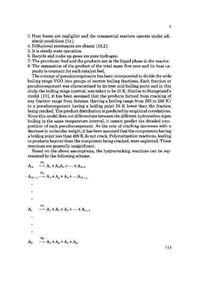
Based on the above assumptions, the hydrocracking reactions can be rep- resented by the following scheme:

H2

AN ' A1+ A2A3 +--- TAN.2

H2

AN-1 "~ AI-t- A2 + A3-f- ---AN_3

H2

Ai ' AI+A2+A3+- - -+Ai_2

H2

A6 ' AI+A2+A3+A4 (1)

where Ag is the component undergoing cracking. A1,A2 ..... A~_ 2 are the products formed from cracking of A~, of which products with i > 6 undergo further hy- drocracking to give still lighter products. Similarly, all the pseudocomponents having boiling points above 400 K (boiling point of A6 is 400.5 K) undergo cracking. The component numbers 1,2,...,N are in ascending order of boiling range and consequently, molecular weight - - the heaviest pseudocomponent being A N. It may be noted that all the pseudocomponents undergoing hydro- cracking need not be present in the feed. In the present case, the feed to the first stage consisted of components from A13 to A23, whereas the product con- tained pseudocomponents ranging from A1 to A23.

Material balance equations

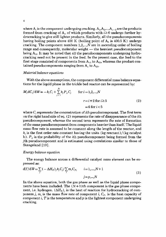
With the above assumptions, the component differential mass balance equa- tions for the liquid phase in the trickle bed reactor can be represented by:

N

MtdC~/dW= -k~C, + ~_, kiPijC j j = r

for i = 1,2,...,N

r=i+2 for i>_5

--6 for i<5

(2)

where Ci represents the concentration of ith pseudocomponent. The first term on the right hand side of eq. ( 2 ) represents the rate of disappearance of the ith pseudocomponent, whereas the second term represents the rate of formation of the same pseudocomponent from components heavier than itself. The liquid mass flow rate is assumed to be constant along the length of the reactor, and ki is the first order rate constant having the units (kg reactant ) / ( kg catalyst h). P~ is the probability of the ith pseudocomponent being formed from the j th pseudocomponent and is estimated using correlations similar to those of Stangeland [ 10 ].

Energy balance equation

The energy balance across a differential catalyst mass element can be ex- pressed as:

dT/dW--~(-AHR)jkjCj/~miCpi i= 1, . . . ,N+ 1 J ' (3)

j = p .... N

In the above equation, both the gas phase as well as the liquid phase compo- nents have been included. The ( N + 1)th component is the gas phase compo- nent, i.e. hydrogen. (AHR)i is the heat of reaction for hydrocracking of com- ponent j, mi is the mass flow rate of component i, Cp i is the heat capacity of component i, T is the temperature and p is the lightest component undergoing cracking.

Correlations for predict ing Pij and ki

The product distribution during hydrocracking of each pseudocomponent was evaluated empirically using correlations similar to those of Stangeland [ 10 ]. The mass fraction of butanes and lighter components formed is given by:

Plj = C exp [ - 0.006 93 ( 1.8tbj - 229.5 ) ] (4)

where tbj is the boiling point of pseudocomponent j ( ° C) and C is a constant. The yield of all other fractions having boiling points higher than that of the butanes were evaluated using one common expression. The entire product boil- ing point range, i.e. starting from the boiling point of the fraction just heavier than the butanes to the boiling point of the heaviest product formed, was first normalized. The normalization equation was

( tbi -2 .5 ) Yii - [(tbj - 5 0 ) -2 .5 ] i = 2 , . . . , j - 2

(5) j = 6 , . . . , N

where yi1 is the normalized temperature for the ith product formed from j th pseudocomponent. The product distribution could then be calculated using the expression:

Ply = [Y~ 3 2 ' +B(y~i - y ~ ) ] [ 1 - P l i ] (6)

where P~j is the cumulative yield till the ith pseudocomponent from hydro- cracking of the j th pseudocomponent. The actual yield of the pseudocompo- nent i from component j was then obtained by subtracting P~_ 1,j from P~i, i.e.

P~J =P~i --P~-l,j (7)

The shape of the product distribution curve depends on the parameter B which generally varies from - 2 to 1. When B = 0, the product distribution is linear. For B = - 2, the probability of the molecule breaking into two equal halves is the maximum. The parameters, B and C depend on the paraffin content of the feed and the type of catalyst.

The rate constant, k~, is highly dependent on the type of hydrocarbon. For instance, the rate of cracking of n-paraffins is less than the rate of cracking of aromatics, cycloparaffins and isoparaffins of the same carbon number. Several kinetic studies on hydrocracking of n-paraffins and some petroleum oils have been published, but their application becomes limited because of the different reaction conditions and the catalyst used. The size, shape and past history of the catalyst are also likely to affect the reaction rate. In the absence of an appropriate rate equation, generally the simplest form of rate expression is assumed. In the present model, the individual rate constants for the pseudo- components were calculated by developing a relative rate function together

1.9

~ 1.?

t~1-5

=.

O

0.9 f

I I I I I L I ~ J J L ~ I J I ~ I 6 8 10 12 14 16 18 20 22

P s e u d o - c o m p o n e n t n u m b e r

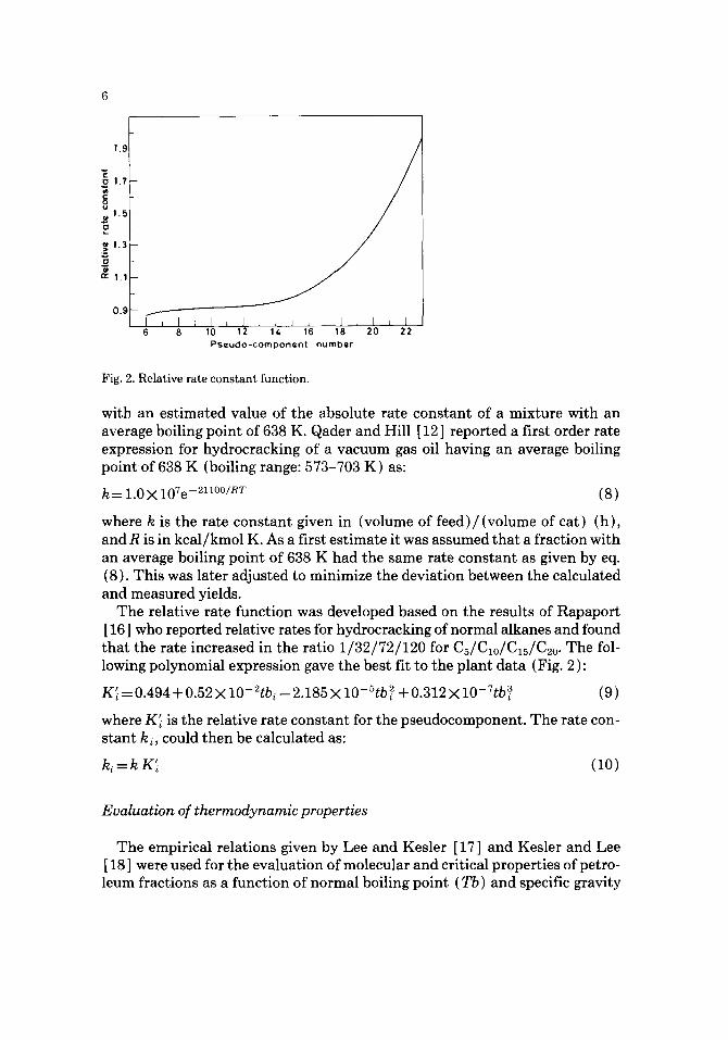
Fig. 2. Relative rate cons tan t function.

with an est imated value of the absolute rate constant of a mixture with an average boiling point of 638 K. Qader and Hill [ 12 ] reported a first order rate expression for hydrocracking of a vacuum gas oil having an average boiling point of 638 K (boiling range: 573-703 K) as:

k = 1.0 X 107e - 2 i IO0/RT (8)

where k is the rate constant given in (volume of f eed) / (vo lume of cat) (h), and R is in kcal /kmol K. As a first est imate it was assumed that a fraction with an average boiling point of 638 K had the same rate constant as given by eq. (8). This was later adjusted to minimize the deviation between the calculated and measured yields.

The relative rate function was developed based on the results of Rapaport [ 16 ] who reported relative rates for hydrocracking of normal alkanes and found that the rate increased in the ratio 1 /32 /72/120 for C5/Clo/C15/C2o. The fol- lowing polynomial expression gave the best fit to the plant data (Fig. 2 ):

K~ -- 0.494 + 0.52 × 10- 2tbi - 2.185 × 10-~tb ~ + 0.312 × 10- 7tb~ (9)

where K~ is the relative rate constant for the pseudocomponent. The rate con- stant ki, could then be calculated as:

k i=k K~ (10)

Evaluation of thermodynamic properties

The empirical relations given by Lee and Kesler [17] and Kesler and Lee [ 18] were used for the evaluation of molecular and critical properties of petro- leum fractions as a function of normal boiling point (Tb) and specific gravity

(SG). The details are given elsewhere [19]. For the calculation of heat capac- ity and enthalpy of the pseudocomponents, the Peng-Robinson equation of state (EOS) is used (Peng and Robinson [20] ). The cubic EOS can be solved for compressibility factor using the method given in Perry's Chemical Engi- neers' Handbook [21 ]. The fugacity coefficient, defined as the ratio of the fu- gacity of a material to its pressure can readily be calculated from the P V T data [22].

The excess enthalpy, H~ ex, for a pure component i is related to its fugacity coefficient (¢i) by the thermodynamic relation:

H~ ex =H~--H~idl = - R T 2(~ ~i (11) In OT

H~ ex H e~ - - - (12)

(MW)i

where H~ is the enthalpy of the ith component in kJ /kmol at any temperature T, H~ x is the excess enthalpy of component i in kJ /kg and R has the units k J / kmol K. The excess enthalpy for a mixture H~ * is related to the partial fugac- ity coefficient ~i by the following relation:

H~ x = H " - - S ' i 2 l = -RT2~. [(a In ~)i)/c)V] (13)

H~ ~ e x Hm - (14)

(MW)

where H " is the enthalpy of the mixture, Hrimdl is the ideal gas enthalpy of the mixture having the units kJ /kmol and H ~ is the excess enthalpy for the mix- ture in kJ/kg. The ideal gas enthalpy, H~ i$, is calculated using the correlation given by Weir and Eaton [23] for enthalpy of vapour above 273 K and low pressures. The heat capacity of the component i (Cpi) and of a mixture (Cp.,) can be obtained from eqs. (15) and (16), respectively.

Cp, = H ~ / [ ( T - 2 7 3 ) (MW)i) ] (15)

Cp m = S ' / [ ( T - 273) (MW)~) ] (16)

where Cp, and Cp~ are in kJ /kg K.

Heats of reaction

The heats of reaction for this system could not be calculated using the stan- dard heats of combustion because of the undefined composition of the reaction mixture. The heats of reaction were calculated on the basis of stoichiometric hydrogen required for each reaction assuming that 42 MJ of heat is released per kmol of hydrogen consumed. This agrees well with the calculated value of 42 MJ per kmol of hydrogen consumed as the standard heat of reaction for hydrocracking of n-hexadecane using the available heats of combustion data

[24]. To estimate the hydrogen consumption, the carbon-to-hydrogen (C/H) ratio of each pseudocomponent and the values of Pijs are required. The C /H ratio data was taken from literature [25,26].

If R'i is the C /H ratio of component i, the total carbon content in the prod- ucts formed from component j, (TWC) 1, which is also equal to the carbon con- tent of component j, W'c,/, can be written as:

( TWC)j =J~ 2 R~ P ij - W 'c,2 j = 6,...,N (17) i=1 R i + l

Similarly the hydrogen content in the products formed from the component j can be written as:

j - 2 1 (TWH) j= Z Pij_, j=6,.. . ,N (18)

i=1 R i + l

Therefore the hydrogen consumption per unit mass of component j can be written as:

( TWH) i - W'c,j/Rj. (19) ( H 2 C R ) i - W'c,j[l+ (1/R~)]

Hence the standard heat of reaction for the j th reaction, (AH ° )j is expressed as :

(AH°)j = (H2CR)j ( -42)103/2 kJ /kg hydrocarbon j=6, . . . ,N (20)

To account for the effect of temperature and pressure on the heat of reaction, the enthalpy of the reactants and the products at reaction temperature and pressure, Hi, was estimated using the Peng-Robinson EOS and at reference conditions, H °, using the correlation formulated by Zhvanestskii and Platnov [22] for liquid hydrocarbon mixtures. For butanes and lighter hydrocarbons, which are not in the liquid state at the reference conditions, the enthalpy was calculated from the heat capacity of butanes (C~1) taken from literature [27]. The enthalpy of hydrogen at reaction conditions (HH2) as well as at standard conditions (H°2) were calculated from the available heat capacity data [28]. The heat of reaction at reaction condition, (AH T )j, can be finally written as

j--2 (AHT)j = (AH° )j + [ ~ ( H i - H ° ) P i j - ( H j - H °) W ' j ( 1 + 1/R~)

i ~ l

- (HH~-H°~)[ (TWH)i -W'~ , j /R ' j ] / [W~, j ( I+I /R~)] j--6,...,N (21)

The set of equations from eqs. (1) to (21) form the mathematical model for the hydrocracking reactor. The total number of equations depends on the num- ber of pseudocomponents.

APPLICATION OF T H E MODEL

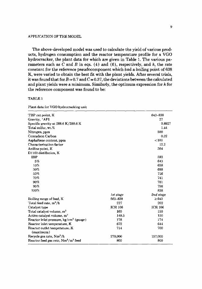
The above-developed model was used to calculate the yield of various prod- ucts, hydrogen consumption and the reactor temperature profile for a VGO hydrocracker, the plant data for which are given in Table 1. The various pa- rameters such as C and B in eqs. (4) and (6), respectively, and k, the rate constant for the reference pseudocomponent which had a boiling point of 638 K, were varied to obtain the best fit with the plant yields. After several trials, it was found that for B = 0.7 and C = 0.37, the deviations between the calculated and plant yields were a minimum. Similarly, the optimum expression for k for the reference component was found to be:

TABLE 1

Plant data for VGO hydrocracking unit

T B P cut point, K Gravity, °API Specific gravity at 288.6 K/288.6 K Total sulfur, wt.% Nitrogen, ppm Conradson Carbon Asphaltene content, ppm Characterization factor Aniline point, K D 1160 distillation, K

IBP 5%

10% 30% 50% 70% 90% 95%

100%

Boiling range of feed, K Total feed rate, m3/h Catalyst type Total catalyst volume, m 3 Active catalyst volume, m 3 Reactor inlet pressure, kg/cm 2 (gauge) Reactor inlet temperature, K Reactor outlet temperature, K

(maximum) Recycle gas rate, Nm3/h Reactor feed gas rate, Nm3/m 3 feed

lststage 563-838

227 ICR106

160 149.5 178 672 714

270,000 800

643-838 27

0.8927 1.44

500 0.32

< 100 12.2

364

593 643 658 688 716 741 781 798 838

2nd stage _> 643

202 ICR 106

150 150 174 644 7OO

157,000 800

10

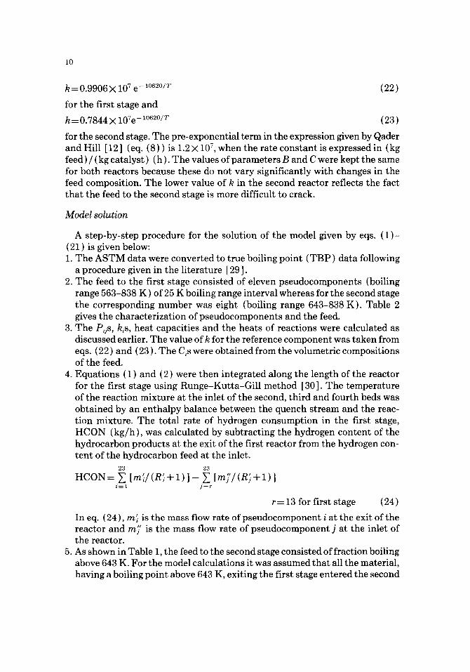
k = 0.9906 X 107 e- 10620/T (22)

for the first stage and

k = 0.7844 X 10re- 10620/T ( 2 3 )

for the second stage. The pre-exponential term in the expression given by Qader and Hill [ 12 ] (eq. (8)) is 1.2 X 107, when the rate constant is expressed in (kg feed ) / (kg catalyst ) (h). The values of parameters B and C were kept the same for both reactors because these do not vary significantly with changes in the feed composition. The lower value of k in the second reactor reflects the fact that the feed to the second stage is more difficult to crack.

Model solution

A step-by-step procedure for the solution of the model given by eqs. (1)- (21) is given below: 1. The ASTM data were converted to true boiling point (TBP) data following

a procedure given in the literature [ 29 ]. 2. The feed to the first stage consisted of eleven pseudocomponents (boiling

range 563-838 K) of 25 K boiling range interval whereas for the second stage the corresponding number was eight (boiling range 643-838 K). Table 2 gives the characterization of pseudocomponents and the feed.

3. The Pijs, kis, heat capacities and the heats of reactions were calculated as discussed earlier. The value of k for the reference component was taken from eqs. (22) and (23). The C/s were obtained from the volumetric compositions of the feed.

4. Equations (1) and (2) were then integrated along the length of the reactor for the first stage using Runge-Kutta-Gill method [30]. The temperature of the reaction mixture at the inlet of the second, third and fourth beds was obtained by an enthalpy balance between the quench stream and the reac- tion mixture. The total rate of hydrogen consumption in the first stage, HCON (kg/h), was calculated by subtracting the hydrogen content of the hydrocarbon products at the exit of the first reactor from the hydrogen con- tent of the hydrocarbon feed at the inlet.

23 23

HCON= ~ [m~/ (R} + l ) ] - ~ [my/ (R~ + l ) ] i=1 j = r

r= 13 for first stage (24)

In eq. (24), rn~ is the mass flow rate of pseudocomponent i at the exit of the reactor and mj' is the mass flow rate of pseudocomponent j at the inlet of the reactor.

5. As shown in Table 1, the feed to the second stage consisted of fraction boiling above 643 K. For the model calculations it was assumed that all the material, having a boiling point above 643 K, exiting the first stage entered the second

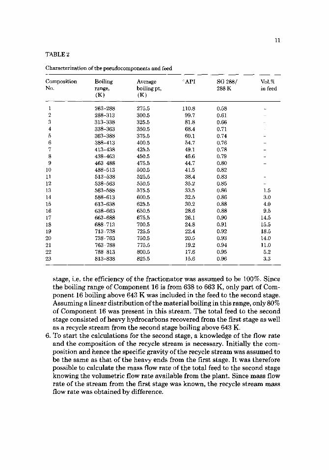
T A B L E 2

Characterization of the pseudocomponents and feed

11

Composition Boiling Average No. range, boiling pt,

(K) (K)

°API SG 288/ 288 K

VoI.% in feed

1 263-288 275.5 110.8 0.58 2 288-313 300.5 99.7 0.61 3 313-338 325.5 81.8 0.66 4 338-363 350.5 68.4 0.71 5 363-388 375.5 60.1 0.74 6 388-413 400.5 54.7 0.76 7 413-438 425.5 49.1 0.78 8 438-463 450.5 46.6 0.79 9 463-488 475.5 44.7 0.80

10 488-513 500.5 41.5 0.82 11 513-538 525.5 38.4 0.83 12 538-563 550.5 35.2 0.85 13 563-588 575.5 33.5 0.86 14 588-613 600.5 32.5 0.86 15 613-638 625.5 30.2 0.88 16 638-663 650.5 28.6 0.88 17 663-688 675.5 26.1 0.90 18 688-713 700.5 24.8 0.91 19 713-738 725.5 22.4 0.92 20 738-763 750.5 20.5 0.93 21 763-788 775.5 19.2 0.94 22 788-813 800.5 17.6 0.95 23 813-838 825.5 15.6 0.96

1.5 3.0 4.0 9.5

14.5 15.5 18.5 14.0 11.0 5.2 3.3

stage, i.e. the efficiency of the fractionator was assumed to be 100%. Since the boiling range of Component 16 is from 638 to 663 K, only part of Com- ponent 16 boiling above 643 K was included in the feed to the second stage. Assuming a linear distribution of the material boiling in this range, only 80% of Component 16 was present in this stream. The total feed to the second stage consisted of heavy hydrocarbons recovered from the first stage as well as a recycle stream from the second stage boiling above 643 K.

6. To start the calculations for the second stage, a knowledge of the flow rate and the composit ion of the recycle stream is necessary. Initially the com- position and hence the specific gravity of the recycle stream was assumed to be the same as that of the heavy ends from the first stage. It was therefore possible to calculate the mass flow rate of the total feed to the second stage knowing the volumetric flow rate available from the plant. Since mass flow rate of the stream from the first stage was known, the recycle stream mass flow rate was obtained by difference.

12

7. Equations (2) and (3) were integrated for the second stage using the same procedure as for the first stage.

8. The mass flow rate and composition of the recycle stream from the second stage were calculated and compared with the assumed value. Successive sub- stitution method was used to update the composition of the recycle stream until convergence was achieved within the preassigned tolerance limit.

9. To compare the calculated yields with the plant data which were available only in four fractions namely high speed diesel (523-643 K), aviation tur- bine fuel (413-523 K), naphtha (288-413 K) and butanes and lighter frac- tions ( < 288 K), it was necessary to group the pseudocomponents into cor- responding boiling ranges assuming a linear distribution.

RESULTS AND DISCUSSION

A general program for the above model was written in Fortran-IV and was executed on a DEC 1090 system. The CPU time required was 2 min 6 s.

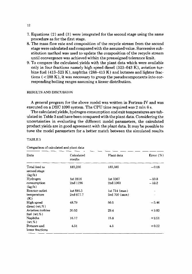
The calculated yields, hydrogen consumption and exit temperatures are tab- ulated in Table 3 and have been compared with the plant data. Considering the uncertainties in evaluating the different model parameters, the calculated product yields are in good agreement with the plant data. It may be possible to tune the model parameters for a better match between the simulated results

T A B L E 3

Comparison of calculated and plant data

Data Calculated Plant data Error (%) results

Total feed to 183,236 183,385 - 0.08 second stage (kg/h) Hydrogen 1st 2816 1st 3267 - 13.8 consumption 2nd 1196 2nd 1363 - 12.2 (kg/h) Reactor outlet 1st 693.3 1st 714 (max) - temperature 2nd 677.7 2nd 700 (max) - (K) High speed 48.79 50.5 - 3.46 diesel (wt.%) Aviation turbine 30.53 29.4 + 3.83 fuel (wt.%) Naphtha 16.17 15.8 + 2.51 (wt.%) Butanes and 4.51 4.5 + 0.22 lower fractions

13

and plant data. However, due to the paucity of extensive experimental data, this was not attempted.

The error in predicting the hydrogen consumption was significant, with the calculated values being lower than the plant values for both the stages. One possible reason for this discrepancy could be due to the fact that hydrodesul- furization and hydrodenitrogenation reactions have not been included in this model. The sulfur content of the feed was 1.44 wt.%. If dibenzothiophene is taken as the representative sulfur compound in the feed, 4 moles of hydrogen would be required to hydrogenate one mole of dibenzothiophene. Thus, for desulfurization, 730 kg of hydrogen would be required which amounts to ap- proximately 16% of the total hydrogen consumption. The sulfur concentration at the exit of each reactor was not known, hence the chemical hydrogen con- sumption for the desulfurization reactions could not be calculated. Another reason for the calculated values of the hydrogen consumption being lower can be attributed to the method of calculating the C/H ratio of the pseudocompo- nents which does not explicitly account for the actual hydrocarbon types pres- ent in a particular boiling range.

As can be seen from Table 3, the calculated feed to the second stage reactor matches almost exactly with the experimental values, thus further validating the model. The calculated temperatures at the outlet of the first stage and second reactors are also shown in Table 3. Since the actual exit values of the temperatures were not available, these could not be compared but are within the specified maximum design limits.

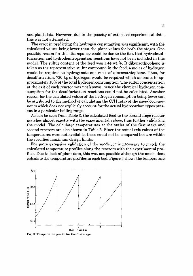
For more extensive validation of the model, it is necessary to match the calculated temperature profiles along the reactors with the experimental pro- files. Due to lack of plant data, this was not possible although the model does calculate the temperature profiles in each bed. Figure 3 shows the temperature

700

~: 69C

"6

E 680 #

67C I I P I

0 1 2 Bed number

Fig. 3. T e m p e r a t u r e p ro f i l e f o r the f i r s t stage.

Y f I 3 4

14

profile along the length of the first reactor. The steep gradients are due to the highly exothermic nature of the hydrocracking reactions. Since the reactor has been assumed to be adiabatic, the profiles for each bed are approximately par- allel, with the temperature dropping due to hydrogen quenching between the catalyst beds. The temperature rise in successive catalyst beds decreases be- cause the rate of hydrocracking is lowered as the average molecular weight of the reactants is reduced due to reaction.

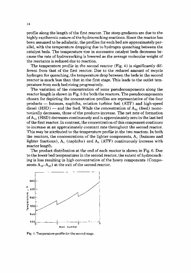
The temperature profile in the second reactor (Fig. 4) is significantly dif- ferent from that of the first reactor. Due to the reduced amount of recycle hydrogen for quenching, the temperature drop between the beds in the second reactor is much less than that in the first stage. This leads to the outlet tem- perature from each bed rising progressively.

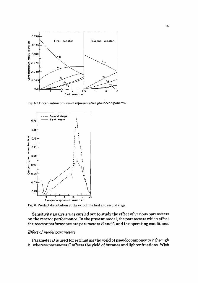
The variation of the concentration of some pseudocomponents along the reactor length is shown in Fig. 5 for both the reactors. The pseudocomponents chosen for depicting the concentration profiles are representative of the four products - - butanes, naphtha, aviation turbine fuel (ATF) and high-speed diesel (HSD) - - and the feed. While the concentration of A2o (feed) mono- tonically decreases, those of the products increase. The net rate of formation of A~4 (HSD) decreases continuously and is approximately zero in the last bed of the first reactor. In contrast, the concentration of this component continues to increase at an approximately constant rate throughout the second reactor. This may be attributed to the temperature profile in the two reactors. In both the reactors, the concentrations of the lighter components, A1 (butanes and lighter fractions), A4 (naphtha) and A9 (ATF) continuously increase with reactor length.

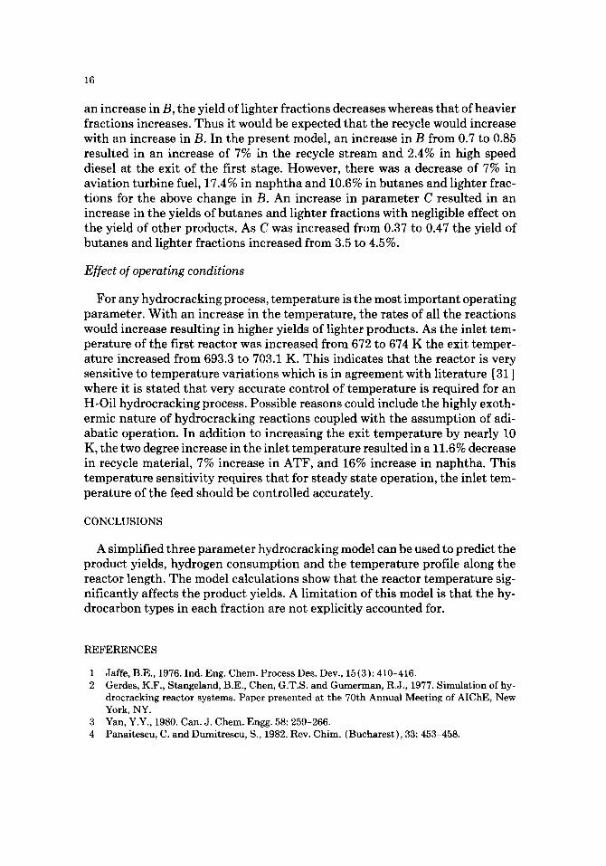
The product distribution at the end of each reactor is shown in Fig. 6. Due to the lower bed temperatures in the second reactor, the extent of hydrocrack- ing is less resulting in high concentration of the heavy components (Compo- nents A16-A23) at the exit of the second reactor.

680

~ 6 7 0

~ 6 6 0

E 650 2

640

630 L l _ _ , I , t 2

Bed number

Fig. 4. Temperature profile for the second stage.

15

0 . 1 5 ( -

F i r s t r e a c t o r S e c o n d r e a c t o r io,,:\ o,oo:

~u 0.050

°° 0.025

0'00 I 2 3 6 0 1 2 ~4 3 Bed n u m b e r

Fig. 5. Concentration profiles of representative pseudocomponents.

0.t7 -- - -

0.1~

. L R 0.13 u a

~ 0.1

E E 0.0~ .2

"~ 0.07

~ 0 . 0 5

0.03

0.Ol

Second stage First stage II

i t t 1 I

i

i _ 11 ~

ir ~111 lJ

3 ? 11 15 19 23 Pseudo-component n u m b e r

Fig. 6. Product distribution at the exit of the first and second stage.

Sensitivity analysis was carried out to study the effect of various parameters on the reactor performance. In the present model, the parameters which affect the reactor performance are parameters B and C and the operating conditions.

Ef[ect of model parameters

Parameter B is used for estimating the yield ofpseudocomponents 2 through 21 whereas parameter C affects the yield of butanes and lighter fractions. With

16

an increase in B, the yield of lighter fractions decreases whereas that of heavier fractions increases. Thus it would be expected that the recycle would increase with an increase in B. In the present model, an increase in B from 0.7 to 0.85 resulted in an increase of 7% in the recycle stream and 2.4% in high speed diesel at the exit of the first stage. However, there was a decrease of 7% in aviation turbine fuel, 17.4% in naphtha and 10.6% in butanes and lighter frac- tions for the above change in B. An increase in parameter C resulted in an increase in the yields of butanes and lighter fractions with negligible effect on the yield of other products. As C was increased from 0.37 to 0.47 the yield of butanes and lighter fractions increased from 3.5 to 4.5%.

Effect of operating conditions

For any hydrocracking process, temperature is the most important operating parameter. With an increase in the temperature, the rates of all the reactions would increase resulting in higher yields of lighter products. As the inlet tem- perature of the first reactor was increased from 672 to 674 K the exit temper- ature increased from 693.3 to 703.1 K. This indicates that the reactor is very sensitive to temperature variations which is in agreement with literature [31 ] where it is stated that very accurate control of temperature is required for an H-Oil hydrocracking process. Possible reasons could include the highly exoth- ermic nature of hydrocracking reactions coupled with the assumption of adi- abatic operation. In addition to increasing the exit temperature by nearly 10 K, the two degree increase in the inlet temperature resulted in a 11.6% decrease in recycle material, 7% increase in ATF, and 16% increase in naphtha. This temperature sensitivity requires that for steady state operation, the inlet tem- perature of the feed should be controlled accurately.

CONCLUSIONS

A simplified three parameter hydrocracking model can be used to predict the product yields, hydrogen consumption and the temperature profile along the reactor length. The model calculations show that the reactor temperature sig- nificantly affects the product yields. A limitation of this model is that the hy- drocarbon types in each fraction are not explicitly accounted for.

REFERENCES

1 Jaffe, B.E., 1976. Ind. Eng. Chem. Process Des. Dev., 15(3): 410-416. 2 Gerdes, K.F., Stangeland, B.E., Chen, G.T.S. and Gumerman, R.J., 1977. Simulation of hy-

drocracking reactor systems. Paper presented at the 70th Annual Meeting of AIChE, New York, NY.

3 Yan, Y.Y., 1980. Can. J. Chem. Engg. 58: 259-266. 4 Panaitescu, C. and Dumitrescu, S., 1982. Rev. Chim. (Bucharest), 33: 453-458.

17

5 Panaitescu, C. and Dumitrescu, S., 1983. Rev. Chim. (Bucharest), 34: 724-727. 6 Langlois, G.E. and Sullivan, R.F., 1970. Chemistry of Hydrocracking, Adv. Chem. Ser., no.

9, pp. 38-67, Am. Chem. Soc., Washington, DC. 7 Goldfarb, Y.Y., Katsobashvili, Y.R. and Rozenthal, A.L., 1981. Kinet. Katal., 22: 668-674. 8 Steijns, M., Froment, G., Jacobs, P. and Uytterhoeven, J., 1981. Ind. Eng. Chem. Prod. Res.

Dev., 20(4): 654-660. 9 Vansina, H., Baltanos, M.A. and Froment, G.F., 1983. Ind. Eng. Prod. Res. Dev., 22: 526-

531. 10 Stangeland, B.E., 1974. Ind. Eng. Chem. Process Des. Dev., 13(1): 71-76. 11 Krishna, R. and Saxena, A.K., 1989. Chem. Eng. Sci., 44(3): 703-712. 12 Qader, S.A. and Hill, G.R., 1969. Ind. Eng. Chem. Process Des. Dev., 8 (1): 98-105. 13 EI-Kady, F.Y.A., 1979. Ind. J. Technol., 17: 176-183. 14 Satterfield, C.N., 1975. AIChE J., 21(2): 209-228. 15 Scott, J.W. and Bridge, A.G., 1971. Continuing Development of Hydrocracking, Adv. Chem.

Ser., No. 103, pp. 113-129, Am. Chem. Soc., Washington, DC. 16 Rapaport, I.B., 1962. Chemistry and Technology of Synthetic Liquid Fuels, Israel Program

for Scientific Translation, Ltd, Jerusalem, 2nd edition. 17 Lee, B.I. and Kesler, M.G., 1975. AIChE J., 21 (3): 510-527. 18 Kesler, M.G. and Lee, B.I., 1976. Hydrocarbon Processing, 55(3): 153-158. 19 Mohanty, S., 1989. Modeling and simulation of hydrocracking and hydrotreating processes,

Ph.D. thesis, Indian Institute of Technology, Kanpur. 20 Peng, D.Y. and Robinson, D.B., 1976. Ind. Eng. Chem. Fundam., 15: 59-64. 21 Perry, R.H. and Green, D.W. (Eds.), 1984. Perry's Chemical Engineers' Handbook. McGraw-

Hill Book Co., New York, NY, 6th edition. 22 Walas, S.H., 1985. Phase Equilibria in Chemical Engineering. Butterworth, Boston, MA. 23 Weir, H.M. and Eaton, G.L., 1932. Ind. Eng. Chem., 24: 211-218. 24 Smith, J.M. and Van Ness, H.C., 1984. Introduction to Chemical Engineering Thermody-

namics. McGraw-Hill, New York. 25 API Technical Data Handbook - Petroleum Refining, 1977, Am. Petr. Inst., Refining Dept.,

Washington, DC. 26 Nelson, W.L., 1958. Petroleum Refinery Engineering. McGraw-Hill, New York, NY, 4th edi-

tion, pp. 169-171. 27 Reid, R.C., Prausnitz, J.M. and Sherwood, T.K., 1977. The Properties of Gases and Liquids.

McGraw-Hill, New York, NY, 3rd edition. 28 Vargaftik, N.B., 1975. Tables on the Thermophysical Properties of Liquids and Gases. Wiley,

New York, NY. 29 Edmister, W.C., 1988. Applied Hydrocarbon Thermodynamics, Vol. 2 Gulf Publishing Co.,

Houston, TX, 2nd edition. 30 Ralston, A. and Wilf, H.S., 1960. Mathematical Methods for Digital Computers. Wiley, New

York, NY, Vol. I. 31 Rapp, L.M. and Van Driesen, R.P., 1969. H-oil process gives product flexibility. In: Hydro-

cracking Handbook, Hydrocarbon Processing, Houston, TX.