Modeling Interdependent Consumer Preferences

Sha Yang

Stern School of Business New York University

44 West Fourth Street, Suite 9-77 New York, NY 10012

Tel: 212-998-0519 shayang@stern.nyu.edu

Greg M. Allenby

Fisher College of Business The Ohio State University

2100 Neil Avenue Columbus, OH 43210-1144

Tel: 614-292-9452 allenby.1@osu.edu

November, 2001 July, 2002

September, 2002

We thank the Editor and reviewers for their constructive comments and suggestions. We also thank seminar participants at University of California – Berkeley, New York University, Cornell University, Hong Kong University of Science and Technology, National University of Singapore, University of Connecticut, Case Western Reserve University, and the University of Wisconsin at Madison for their helpful comments.

Modeling Interdependent Consumer Preferences

Abstract

An individual's preference for an offering can be influenced by the preferences of others

in many ways, ranging from the influence of social identification and inclusion, to the benefits of

network externalities. In this paper, we introduce a Bayesian autoregressive discrete choice

model to study the preference interdependence among individual consumers. The autoregressive

specification can reflect patterns of heterogeneity where influence propagates within and across

networks. These patterns cannot be modeled with standard random-effect specifications, and can

be difficult to capture with covariates in a linear model. Our model of interdependent

preferences is illustrated with data on automobile purchases, where preferences for Japanese

made cars are shown to be related to geographic and demographically defined networks.

1

Modeling Interdependent Consumer Preferences

1. Introduction

Preferences and choice behavior are influenced by a consumer's own tastes and also the

tastes of others. People who identify with a particular group often adopt the preferences of the

group, resulting in choices that are interdependent. Examples include the preference for

particular brands (e.g. Abercrombie and Fitch) and even entire product categories (e.g.

minivans). Interdependence may be driven by social concerns, by endorsements from respected

individuals that increase a brand's credibility, or by learning the preference of others who may

have information not available to the decision maker. Moreover, since people engage in multiple

activities with their families, co-workers, neighbors and friends, interdependent preferences can

propagate across and through multiple networks.

Quantitative models of consumer purchase behavior often do not recognize that

preferences and choices are interdependent. Economic models of choice typically assume that an

individual's latent utility is a function of brand and attribute preferences, not the preferences of

others. Preferences are assumed to vary across consumers in a manner described either by

exogenous covariates, such as demographics (e.g., household income), or by independent draws

from a mixing distribution in random-effects models (see Allenby and Rossi 1999, Kamakura

and Russell 1989). However, if preferences in a market are interdependently determined, their

pattern will not be well represented by a simple linear model of exogenous covariates. Failure to

include high-order interaction terms in the model to reflect interdependent influences will result

in correlated structure of unobserved heterogeneity, where the draws from a random-effects

mixing distribution are dependent, not independent.

2

In this paper, we introduce a Bayesian model of interdependent preferences in a

consumer choice context. We employ a parsimonious autoregressive structure that captures the

endogenous relationship between an individual's preference and the preference of others in the

same network. Our model allows for a complex network associated with multiple explanatory

variables. In addition, our model allows us to incorporate explanatory variables in both an

exogenous and endogenous (i.e., interdependent) manner. A Markov chain Monte Carlo method

is employed to estimate the model parameters.

The remainder of the paper is organized as follows. Section 2 reviews the literature in

economics and marketing on interdependent preference, providing rationale for our model

structure. Section 3 lays out the model and estimation procedure, and section 4 presents a

numerical simulation to assess the accuracy of the model in recovering the true parameter values.

An empirical application of the model is set forth in section 5 to study the interdependence in a

binary choice decision: whether to buy a foreign brand or a domestic brand of mid-sized car.

Section 6 offers concluding comments.

2. Review of Interdependent Preference Studies

People do not live in a world of isolation. They interact with each other when forming

their opinions, beliefs and preferences. Interdependent preference (or preference interaction) has

been defined as “occurring when an agent’s preference ordering over the alternatives in a choice

set depends on the actions chosen by other agents” (Manski 2000). This effect has also been

called "peer influences" (Duncan, Haller and Portes 1968), "neighborhood effects" (Case 1991),

“bandwagon effect” (Leibenstein 1950) and "conformity" (Bernheim 1994) in studies of

interdependence.

3

Interdependent preferences can arise in many ways. Reasons include social concerns,

reductions in transaction costs (i.e., network externalities) and the signaling effect of another's

brand ownership on inferred attribute-levels. In addition, interdependent preferences may

appear to be present in economic demand models in which key explanatory variables are either

omitted (e.g., household income) or unobserved (e.g., media exposure). Our review of the

literature focuses on the former explanation, and the model specification is guided by the

potential mechanisms by which interdependent preference arises. The review below provides a

useful guide to researchers studying the origins of utility.

Pioneering work on interdependent preference was conducted by Duesenberry (1949) and

Leibenstein (1950). Duesenberry described several examples of interdependence in consumer

consumption behavior. Using data on consumer purchases made in 1935-36, he found that the

percentage of income spent on consumption is highly correlated with the person’s rank order in

the local income distribution. Leibenstein (1950) formally incorporated the phenomenon of

"conspicuous consumption" into a theory of consumer demand. Through a conceptual

experiment, he showed that the demand curve will be more elastic if there is a bandwagon effect

than if the demand is based only on the functional attributes of the commodity. Since this work,

a large body of literature has emerged that has examined the theory and empirical evidence of

interdependent preference.

Theoretical Research on Interdependent Preference

In the theory domain, Hayakawa and Venieris (1977) derived several utility theories and

axioms for preference interdependence. Their theories predict that the income effect associated

with a price change will become dominant as the budget expenditure is relaxed. Moreover, their

4

research points to the need for a concept of psychological complementarity to capture the role of

reference group in a consumer choice calculus. While Hayakawa and Venieris’s framework is

mainly static, several other papers have tried to address the influence of preference

interdependence adding a temporal dimension. For example, Cowan, Coman and Swann (1997)

derived the steady state and dynamic properties of the distribution of consumption when

different reference groups were used. Bernheim (1994) suggests a theory of how standards of

behavior might evolve in response to changes in the distribution of intrinsic preferences.

While the focus of studying the interdependent effects in economics is mainly on its

impact on demand theory and econometric implications, researchers in the marketing have paid

more attention to explaining the mechanisms of the interdependent preferences among

consumers in the context of reference group formation and influence. These two areas of

research are distinguished. The first examines the reasons that individuals conform to the

behavior of a reference group. Researchers have identified three sources of social influence on

buyer behavior: internalization, identification and compliance (Kelman 1961; Burnkrant and

Consineau 1975; Lessig and Park 1977). Internalization occurs when a person adopts other

people’s influence because it is perceived to "inherently conductive to the maximization of his

value." In other words, people are willing to learn from others in a sense that this could help

them make a better decision that optimizes their own returns. Identification occurs when

adopting from others because the "behavior is associated with a satisfying self-defining

relationship" to the other. Compliance occurs when "the individual conforms to the expectations

of another in order to receive a reward or avoid punishment mediated by that other."

The second area of research in marketing examines the relative influence of alternative

mechanisms on individual consumer behavior. Bearden and Etzel (1982) studied how reference

5

groups influence an individual consumer’s purchase decisions at both product and brand level.

Lessig and Park (1982) showed that the degree of reference group influence is dependent on the

product related characteristics such as complexity, conspicuousness and brand distinction.

Childers and Rao (1992) found that reference-group influence varies for products consumed in

different occasions (public vs. private) and for different reference groups (familial vs. peer).

Interdependent preferences can therefore be associated with multiple covariates, and can

lead to either conformity or individuality in preferences. In the next section we present a model

capable of reflecting these effects, within the framework of an economic choice model.

Measuring Interdependence

In the empirical domain, a considerable amount of effort has been devoted to developing

econometric models and estimation methods that incorporate interpersonal dependence (Pollak

1976; Kapteyn 1977; Stadt, Kapteyn and Geer 1985). Some empirical applications include

studying interdependent preference in consumer expenditure allocations (Darough, Pollak and

Wales 1983; Alessie and Kapteyn 1991; Kaptyen et. al. 1997), labor supply (Aronsson,

Blomquist and Sacklen 1999), rice consumption (Case 1991), and elections (Smith and LeSage

2000). The focus of these studies is typically very aggregate, with the dependent variable

reflecting average behavior (e.g. consumption) within a particular geographic region (e.g. zip

code). Furthermore, they tend to use a single network to model the preference interdependence.

Methodological research in marketing on interdependent preferences has recently been

spurred by developments in simulation-based estimation that facilitate flexible models of

consumer heterogeneity, including models where dependence is spatially related. Arora and

Allenby (1999) propose a conjoint model where the importance of product attributes in a group

6

decision making context can be different from the part-worths of each individual. However,

their model assumes that the social group is readily identified, and does not account for the

possibility of multiple networks. Hofstede, Wedel and Steenkamp (2002) examine the use of

alternative spatial prior distributions to geographically smooth model parameters in a study of

retail store attributes. In their analysis, response coefficients in a geographic area are assumed to

be similar to neighboring areas. Bronnenberg and Mahajan (2001) combine an autoregressive

spatial prior on market shares with a temporal autoregressive process to study variation in the

effectiveness of promotional variables in geographically defined markets. Bronnenberg and

Sismeiro (2002) use a spatial model to forecast brand sales in markets where only limited

information exist. Neither of these later studies are developed to study preferences at the level of

the individual consumer.

In this paper we develop an autoregressive mixture model and apply it to the latent utility

in a discrete choice model. The autoregressive model relates an individual's latent utility to the

utility of other individuals, reflecting the potential interdependence of preferences. Explanatory

variables are incorporated into the autoregressive process through a weighting matrix that

describes the network. The mixture aspect of the model allows the weighting matrix to be

defined by multiple covariates, with covariate importance estimated from the data. Covariates

are also related to the expected value of the latent utilities to capture exogenous, as opposed to

endogenous effects.

3. A Hierarchical Bayes Autoregressive Mixture Model

In this section, we first introduce a binary choice model that captures the potential social

dependency of preferences among individuals. Then we briefly describe the prior distribution

7

specification and estimation procedure using Markov chain Monte Carlo methods. A detailed

description of the estimation algorithm is provided in the appendix.

3.1 An Autoregressive Discrete Choice Model

Suppose we observe choice information for a set of individuals (i = 1,…,m) who are not

associated with an interdependent network and whose preferences are exogenously determined.

Assume that the individual is observed to make a selection between two choice alternatives (yi =

1 or 0) that is driven by the difference in latent utilities, Uik, for the two alternatives (k = 1,2).

The probability of selecting the second alternative over the first is:

)0Pr()Pr()1Pr( 12 >=>== iiii zUUy (1)

iii xz εβ += ' (2)

εi ~ Normal(0,1) (3)

where zi is the latent preference for the second alterative over the first alternative, xi is a vector of

covariates that captures the differences of the characteristics between the two choice alternatives

and characteristics of the individual, β is the vector of coefficients associated with xi, and εi

reflects unobservable factors modeled as error. Preference for a durable offering, for example,

may be dependent on the existence of local retailers who can provide repair service when

needed. This type of exogenous preference dependence is well represented by equation (2). The

error term is assumed to be independently distributed across individuals, reflecting the absence

of interdependent effects. The scale of the error term is equal to one to statistically identify the

8

model coefficients, β. Stacking the latent preferences, zi, into a vector results in a multivariate

specification:

z ~ Normal(Xβ,I) . (4)

The presence of interdependent networks creates preferences that are endogenous and

mutually dependent, resulting in an error covariance matrix (Σ) with non-zero off diagonal

elements. The presence of off-diagonal elements in the covariance matrix leads to conditional

and unconditional expectations of preferences that differ. The expectation of latent preference, z,

in equation (4) is equal to Xβ regardless of whether preferences of other individuals are known.

However, if the off-diagonal elements of the covariance matrix are non-zero, then the conditional

expectation of the latent preference for one individual is correlated with the revealed preference

of another individual:

E[z2|z1] = X2'β + Σ21Σ11-1(z1-X1β) , (5)

where the subscripts apply to appropriate elements of the parameters. Positive covariance leads

to a greater expectation of preference z2 if it is known that z1 is greater than its mean, X1β. In the

probit model, choice (yi) is revealed, corresponding to a range of latent preferences (i.e., zi > 0).

The computation of conditional expectation is therefore associated with an integration over a

range of possible conditioning arguments.

An approach to inducing covariation among the error terms is to augment the error term

in equation (2) with a second error term from an autoregressive process (LeSage 2000):

9

zi = xi'β + ε + θi (6)

θ = ρWθ + u (7)

ε ~ N(0,I) (8)

u ~ N(0,σ2I) (9)

where ε and u are iid error terms, θ is a vector of autoregressive parameters where the matrix ρW

reflects the interdependence of preferences across individuals. The specification in equation (7)

is similar to that encountered in time series analysis, except that co-dependence can exist

between two elements, whereas in time series analysis the dependence is directional (e.g., an

observation at time t-k can affect an observation at time t, but not vice versa). Co-dependence is

captured by non-zero entries appearing in both the upper and lower triangular sub-matrices of W.

It is assumed that the diagonal elements wii are equal to zero and each row sums to one. The

coefficient ρ measures the degree of overall association among the units of analysis beyond that

captured by the covariates, X. Positive (negative) value of ρ indicates positive (negative)

correlation among people.

It is worth noting that in our model of interdependent preferences, there is a network

propagation effect captured in equation (7), where in the exogenous model the effect associated

with a covariate does not propagate among consumers. Our model presents a simple test on the

existence of propagation effect. If ρ is significantly different from zero, then we conclude that

there could be some interdependent preference beyond what is captured in the x'β term in

equation (6).

The augmented-error model results in latent preferences with non-zero covariance:

10

z ~ Normal(Xβ, I+σ2(I-ρW)-1(I-ρW')-1) . (10)

This specification1 is different from that encountered in standard spatial data models (see Cressie

1991, p.441) where the error term ε is not present and the covariance term is equal to σ2(I-ρW)-1

(I-ρW')-1. The advantage of specifying the error in two parts is that it leads itself to estimation

and analysis using the method of data augmentation (Tanner and Wong, 1987). The

autoregressive parameter θ is responsible for the nonzero covariances in the latent preferences, z,

but is not present in the likelihood specification (equation (10)). By augmenting the parameters

space with θ, we isolate the effects of the non-zero covariances and simplify the evaluation of the

likelihood function (see below).

The elements of the autoregressive matrix, W = wij, reflect the potential dependence

between units of analysis. A critical part of the autoregressive specification concerns the

construction of W. Spatial models, for example, have employed a coding scheme where the un-

normalized elements of the autoregressive matrix equal one if i and j are neighbors and zero

otherwise (see Bronnenberg and Mahajan 2001). An alternative specification for a spatial model

could involve other metrics, such as Euclidean and Manhattan distances. However, as noted

above, interdependent preferences can be determined by multiple networks. It is therefore

important to allow for a specification of the autoregressive matrix, W, with multiple covariates.

1 With this model specification, we assume that θ has smaller variance for people in larger networks. We believe this property is justified. As the size of the network increases, interdependence implies there exists more information about a specific consumer's preference, and hence smaller variance.

11

We specify the autoregressive matrix W as a finite mixture of coefficient matrices, each

related to a specific covariate:

∑=

=K

kkkWW

1

φ , (11)

∑=

=K

kk

1

1φ . (12)

where k indexes the covariates, k = 1,…, K. The weights, φk, reflect the relative importance of

the component matrices, Wk, with each associated with a different explanatory variable. W1, for

example, may be related to the physical proximity of the individual residences, W2 to their age,

W3 to their income, W4 to their ethnicity, and so on. Within each matrix, Wk, the diagonal

elements are assumed equal to zero, the off diagonal elements reflect the distance between

individuals in terms of the kth covariate, and each row sums to one. The weighted sum of them

component matrices, W, also has these properties since the weights, φk, sum to one. In our

specification we re-parameterize φk with a logit specification:

∑=

= K

kk

jj

1)exp(

)exp(

α

αφ (13)

and estimate αj unrestricted with αK = 0.

The model described by equations (1), (6), (7), (8) and (9) is statistically identified. This

can be seen by considering the choice probability Pr(yi =1) = Pr(zi > 0) = Pr(xi'β + εi + θi > 0).

12

The right side of the later expression is zero, and the variance of εi is one. These specifications

identify the probit model in terms of location and scale because an arbitrary constant cannot be

added to the right side of the expression, and multiplying by a scalar quantity would alter the

variance of εi. Moreover, the finite mixture specification described by equation (10), (11) and

(12) is identified because the rows of Wk and the mixture probabilities are normalized to add to

one. However, we note that care must be exercised in comparing estimates of β from the

independent probit model (equation (4)) with that from the autoregressive model (equation (10))

because of the differences in the magnitude of the covariance matrix. We return to the issue of

statistical identification below when demonstrating properties of the model in a simulation study.

Our model is based on the framework developed by Smith and LeSage (2001), but

extends theirs in the following ways. First, the spatial matrix W in their model is constrained to

be only geographic specific. We introduce a more flexible structure to capture different sources

of interdependence across multiple networks. Second, most applications in this area of research,

including Smith and LeSage (2001), focus on zip code level analysis. Our analysis investigates

interdependence at the individual level which is of interest to marketing.

3.2 Prior Specification and Markov chain Estimation

We estimate the autoregressive discrete choice model using Markov chain Monte Carlo

methods. This method of estimation requires specification of prior distributions for the model

parameters in equation (10), and derivation of the full conditional distribution of model

parameters. The prior distributions are set to be diffuse and conjugate when possible. We use

some standard prior distribution specification as follows:

13

),(~ 0 βββ VN (14)

maxmin

1,1~λλ

ρ U (15)

),(~ 0 ααα VN (16)

),(IG~ 002 qsσ (17)

Here, α and β have normal conjugate prior distributions with means set to zero and

covariance matrices set to 100I where I is the identity matrix, and is assigned a conjugate

inverted gamma prior with s

2σ

0 = 5 and q0 = 0.1. We employ a uniform prior distribution on ρ

over a specified range. The parameter ρ must lie in this interval

max

1,λ , where

min

1λ minλ and

maxλ denote the minimum and maximum eigenvalues of W, for the matrix (I - ρW) to be

invertable (Sun, Tsutakawa and Speckman 1999).

The Markov chain proceeds by generating draws from the set of conditional posterior

distributions of the parameters. As mentioned above, we augment the model parameters θ in

equation (7) that capture the dependent error structure through an autoregressive process. By

conditioning on θi, the latent preference, zi, is seen to arise from a standard binomial probit

model with mean xi'β + θi and independent errors. Furthermore, the conditional distributions of

the model parameters, given θ, are of standard form. A detailed description of the full

conditional distributions is provided in Appendix A. We note that generating draws from the full

conditional distribution of θ is computationally demanding, and we adopted the method proposed

14

by Smith and LeSage (2000) to iteratively generate draws for the elements of θ. Appendix B

briefly outlines this method.

4. A Simulation Study

In this section, we demonstrate properties of the autoregressive choice model and

investigate the relationship between sample size and accuracy of the MCMC estimator. We

focus our analysis on the model without the latent mixing distribution described in equation (11)

through equation (13).

4.1 Data Simulation

We simulate three datasets. The first dataset is comprised of 50 individuals and the

second dataset contains 500 individuals. We assume the individuals are connected circularly,

with each individual affected by his/her two closest neighbors. To illustrate, the autoregressive

matrix, W, for five individuals is as follows:

=

05.005.5.05.0005.05.0005.05.5.005.0

W (18)

We assume that X is comprised of two covariates generated from a standard normal distribution,

β' = (1,1)', and 42 =σ 5.0=ρ . Binary choices (yi) are simulated by generating draws from a

multivariate normal distribution specified in equation (10) and applying the censoring described

15

in equation (1). The covariance matrix of the latent preference distribution for the five

individuals described by the autoregressive matrix in equation (18) is:

=′−−+=Σ −−

3.72.36.16.12.32.33.72.36.16.16.12.33.72.36.16.16.12.33.72.32.36.16.12.33.7

)()( 112 WIWII ρρσ (19)

The covariance between the first and third individual is nonzero despite the fact that these

two individuals are not neighbors. The first individual is connected to the second individual and

the second to the third in the autoregressive matrix (equation (18)). The connections induce

nonzero covariance between the first and third individuals, reflecting the correlation of the

circular network. The variances along the diagonal of Σ are equal, reflecting the fact that each

individual has exactly two neighbors. To examine the performance of the estimator for a

heteroskedastic error matrix, we include a third case in which the matrix W is formulated using

data from our empirical study (reported below). This third simulation study contains 666

observations.

4.2 Accuracy of Parameter Estimates

Estimation results are presented in Table 1. We ran the Markov chain for 5000 iterations

and deleted the first 1000 draws for 'burn-in' of the chain. The last 4000 draws were used to

calculate the posterior mean and standard deviation of the parameters. From the table, we see

that the coefficient estimates are close to their true values, even in small samples. As expected,

the true parameters lie inside the 95% highest posterior density intervals of the posterior

16

distributions, and the accuracy of the estimator improves as the sample size increases. We also

ran the Markov chain for 10,000 iterations and found no appreciable difference in the estimates

reported in table 1. These results support our conclusion that the autoregressive choice model is

statistically identified and our estimation using data augmentation is valid.

= = Table 1 = =

The purpose of the autoregressive specification is to understand dependence among

individuals as reflected in the covariance matrix. It is therefore important to investigate the

model's ability to recover the realizations of the choice model error responsible for inducing the

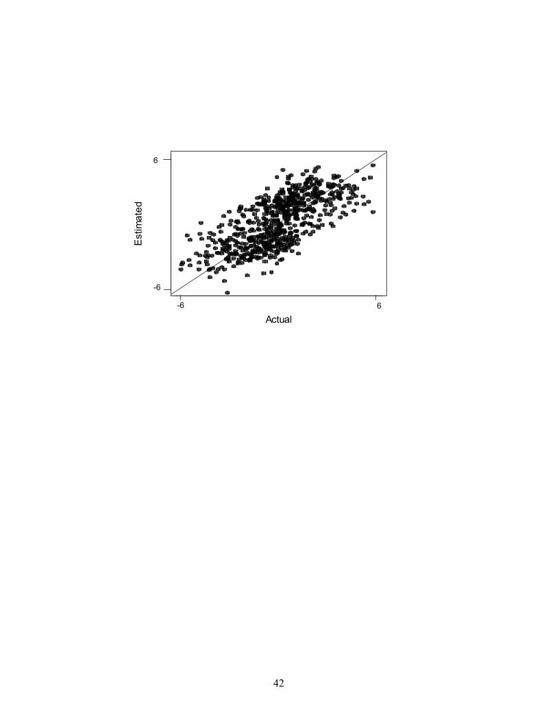
covariances. Figure 1 provides a comparison between the estimated and actual autoregressive

effects (θi). The top panel of figure 1 displays a plot of the estimated and actual autoregressive

effects for the dataset with 50 observations (individuals), the middle panel of figure 1 displays

the plot for the dataset with 500 observations, and the bottom panel of figure 1 displays the plot

for the dataset with 666 observations with spatial interaction generated to mimic our empirical

analysis, described below. Also included in the plots is a 45 degree line. The points in the

graphs tend to fall evenly about the line, indicating that the estimated autoregressive effects are

not biased. Moreover, the variability of the points about the line does not depend appreciably on

the sample size. An increase in the sample size results in improved estimates of the model

parameters in table 2, but not in terms of the augmented parameter θi, because the dimension of θ

is the same as the number of observations in the analysis. Our analysis indicates that, despite the

sparseness present in a circularly connected population of 500 people, or present in our data

reported below, accurate estimates of model parameters, including the augmented parameters θ,

are possible.

17

The autoregressive effects are used to assess the degree of dependence in the probit error

structure. If there is little interdependence in consumer choice, or if the data is not sufficiently

informative about the presence of interdependencies, then the realizations of θi will be near zero

and the predicted choice probabilities, conditional on θi, will be similar to that obtained from an

independent probit specification (Σ = I). If choice and preferences are interdependent, then the

realizations of θi will be large and there will exist improvements in model fit by conditioning on

the dependent information contained in θi.

= = Figure 1 = =

4.3 Assessing Differences in Regression Coefficients

The presence of an autoregressive component in the error term changes the variance of

the probit model from the identity matrix to Σ = I + σ2(I-ρW)-1(I-ρW')-1. As illustrated in

equation (19), the autoregressive specification can lead to large changes in the diagonal elements

of the covariance matrix. Care must therefore be exercised when interpreting the regression

coefficients associated with the mean of the multivariate normal distribution. Although we have

demonstrated that the autoregressive specification leads to an identified model, these coefficients

must be interpreted relative to the scale of the error term. This is most easily accomplished by

computing the expected change in the choice probability for a change in the independent

variable.

Table 2 contains the regression coefficient estimates for the dataset with 500 observations

discussed above, along with regression estimates from a traditional binary probit model with Σ =

I (that is, setting all θi to 0). The regression estimates for the autoregressive model are much

larger than those obtained from the independent probit model. However, when these coefficients

18

are converted to expected derivatives of the choice probability at x1 = 0 and x2 = 0, the estimates

for the two models are seen to closely agree. The change in probability is 0.245 for the

independent probit model (equation (4)), and 0.270 for the dependent probit model (equation

(10)) when both x1 and x2 increase from 0.0 to 1.0. Either model is capable of capturing the

average association between the covariates and choice. The autoregressive model, however, is

needed to understand the extent and nature of preference inter-dependencies given the average

association.

= = Table 2 = =

5. Empirical Application

Data were collected by a marketing research company on purchases of mid-sized cars in

the United States. We obscure the identity of the cars for the purpose of confidentiality. The

cars are functionally substitutable, priced in a similar range, and are distinguished primarily by

their national origin: Japanese and non-Japanese. Japanese cars have a reputation for reliability

and quality in the last twenty years, and we seek to understand the extent to which preferences

are inter-dependent among consumers.

We investigate two sources of dependence – geographic and demographic neighbors.

Geographic neighbors are created by physical proximity and measured in terms of geographic

distance among individuals' places of residence. Demographic neighbors are defined in terms of

similar demographic variables. Young people, for example, are more likely to associate with

other young people, obtain information from them, and may want to conform to the beliefs to

their reference group to gain group acceptance and social identity. We empirically test these

referencing structures and analyze their importance in driving the preferences.

19

We operationalize the different referencing schemes as follows. The data include

information on the longitude and latitude information of each person’s residence, and we can

calculate the geographic distance between person i and j as follows:

222211 )()(),( jiji ddddjid −+−= (20)

where denotes the longitude and denotes the latitude of individual j’s home. We further

assume that geographic influence is an inverse function of the geographic distance:

1jd 2

jd

)),(exp(

11

, jidwg

ji = (21)

An alternative geographic specification of W that leads to a symmetric matrix is to identify

neighbors by the zip code of their home mailing address:

1 if person i and person j have the same zip code; 0 otherwise. (22) =2,g

jiw

We operationalize demographic neighbors in terms of people who share characteristics such as

education, age, income, etc. Individuals in the dataset are divided into groups defined by age of

the head of the household (3 categories), annual household income (3 categories), ethnic

affiliation (2 categories) and education (2 categories). This leads us to a maximum of 36 groups,

31 of which are presented in our sample. The demographic specification of W becomes:

20

1 if person i and person j belong to the same demographic group; 0 otherwise.

(23)

=djiw ,

The data consist of 857 consumers who live in 122 different zip codes. Table 3 provides

sample statistics of the data. Approximately 85% of people purchased a Japanese car. On

average, the price a Japanese car is $2400 cheaper than a non-Japanese car and there is little

difference between the optional accessories purchased with the cars. We note, however, that the

sample standard deviations are nonzero, indicating intra-group variation. The average age of the

consumer is 49 years, and average annual household income is approximately $67,000.

Approximately 12% of the consumers are of Asian origin, and 35% have earned a college

degree. The choices of 666 individuals from 100 zip codes are used to calibrate the model, and

191 observations form a holdout sample. Figure 2 is a histogram of the number of zip codes

containing at least two consumers, indicating that the sample of respondents is geographically

dispersed.

= = Table 3 = =

= = Figure 2 = =

In sample and out of sample fit are assessed in the following way. When possible, we

report fit statistics conditional on the augmented parameter θi. For the independent probit model

(equations (1) – (3)) in which θi = 0, the latent preferences are independent after accounting for

the influence of the covariates in mean of the latent distribution (equation (4)). Knowledge that

an individual actually purchased a Japanese car provides no help in predicting the preferences

and choices of other individuals. When preferences are interdependent, information about others'

21

choices is useful in predicting choices, and this information is provided through θi as described

in equation (7).

In-sample fit is assessed using the importance sampling method of Newton and Raftery

(1994, p.21) that re-weights the conditional likelihood of the data. Conditional on θ, this

evaluation involves the product of independent probit probabilities and is easy to compute.

Computing the out of sample fit is more complicated. Our analysis proceeds as it would in

developing a customer scoring model, by constructing the autocorrelation matrices W for the

entire dataset (857 observations), but estimating the model parameters using the first 666

observations. We obtain the augmented parameters for the holdout sample, θp, by noting that

(24)

ΣΣΣΣ

=−−≈

−−

2221

12111857

1857

2 ,0))'ˆˆ()ˆˆ(ˆ,0( NWIWINp ρρσθ

θ

where is the covariance matrix between 12Σ θ and , and we can obtain the conditional

distribution of θ

pθ

p given θ using properties of the multivariate normal distribution:

( ) ),(~| Ωµθθ MNp (25)

where

(26) θµ 11121−ΣΣ=

(27) 121

112122 ΣΣΣ−Σ=Ω −

22

Table 4 reports the in sample and out sample fit statistics for six different models. The

first model is an independent binary probit model (equations 1-3) where the probability of

purchasing a Japanese car is associated with the feature differences between cars, demographics

information for the individual, geographic information (longitude, latitude), and dummy

variables for the demographic groups. The dummy variables can be viewed as an attempt to

capture high-order interactions of the covariates. Dummy variables for only 19 of the 31 groups

are included because the proportion of buyers of Japanese cars in the remaining groups is at or

near 100%. Thus, the first model attempts to approximate the structure of heterogeneity using a

flexible exogenous specification.

The second model is a random-effects model that assumes people living in the same zip

code have identical price and option coefficients. Geographic and demographic variables are

incorporated into the model specification to adjust the model intercept and the mean of the

random-effects distribution. The second model represents a standard approach to modeling

preferences, incorporating observed and unobserved heterogeneity.

Models 3-6 specify four variations of interdependent models in which consumer

preferences are endogenous, or interdependent. Models 3 and 4 are alternative specifications for

geographic neighbors (equations (21) and (22)), whereas Model 5 specifies the autoregressive

matrix in terms of the 31 demographic groups (equation 23). Model 6 incorporates both

geographic and demographic structures using the finite mixture model in equations (11) – (13).

= = Table 4 = =

The model fit statistics (both in sample and out sample) indicate the following. First, car

choices are inter-dependent. Model 1 is the worst fitting model and all attempts into incorporate

geographic and/or demographic interdependence in the model leads to improved in-sample and

23

out-of-sample fit. A comparison of the fit statistics between Model 2 and Models 3-6 indicates

that there is stronger evidence of interdependence in the autoregressive models than in a random-

effects model based on zip codes. Moreover, adding quadratic and cubic terms for longitude and

latitude results in a slight improvement in-sample fit (i.e, from –203.809 to –193.692) and an

out-of-sample fit (i.e., from 0.158 to of 0.154). This supports the view that people have similar

preferences not only because they share similar demographic characteristics that may point to

similar patterns of resource allocation (an exogenous explanation), but also because there is an

endogenous interdependence among people. Furthermore, Model 3 and 4 produce very similar

fit statistics, which indicates that geographic neighbor based weighting matrix performs a good

approximation to geographic distance based weighting matrix. The introduction of both of

geographic and demographic referencing schemes in Model 6 leads to an improvement in the fit,

showing that both reference groups are important in influencing the individual’s preference.

Parameter estimates for the six models are reported in table 5. We note that, in general,

the coefficient estimates are largely consistent across the six models, indicating that all of the

models are somewhat successful in reflecting the data structure. Since Model 6 yields the best

in-sample and out-sample fit, we focus our discussion on its parameter estimates. The estimates

indicate that price, age, income, ethnic origin, longitude and latitude are significantly associated

with car purchases, with Asians, younger people, people with high incomes, and living more

southern and more western preferring Japanese makes of car. The ethnic variable turns out to

have a very large coefficient indicating that Asian people will have a significantly higher

likelihood of choosing a Japanese brand car. Furthermore, ρ is significantly positive indicating

a positive correlation among consumer preferences. α is significantly positive (φ greater than

24

0.5) indicating that geographic reference groups are more important in determining the

individual’s preference compared with demographic reference groups.

= = Table 5 = =

Figure 3 displays estimates of the elements of the augmented parameter θ against the

longitude and latitude of each observation in sample. Most of the estimates have posterior

distributions away from zero, providing evidence of interdependent choices. An analysis of the

difference in covariates for the two groups (θ > 0 and θ ≤ 0) does not reveal any statistically

significant differences except for the longitude variable. That is, the augmented parameters that

capture the endogenous nature of preferences are not simply associated with all the covariates in

the analysis.

= = Figure 3 = =

6. Summary and Concluding Remarks

In this paper we introduce an autoregressive multivariate binomial probit model to study

interdependent choices among individuals. The model is specified in a hierarchical Bayes

framework and estimation algorithms are derived using data augmentation to simplify the

computations. We investigate the influence of two possible sources of interdependent influence:

geographic neighbors and demographic neighbors. Geographic neighbors are individuals who

reside in close proximity to each other, while demographic neighbors are identified by

demographic variables that point to social networks.

Alternative model specifications are used to investigate variation in preferences. We find

that a standard random-effect specification is inferior to an autoregressive specification. In the

random-effect specification, variation in preferences across individuals is modeled as

25

independent draws from a mixing distribution, whereas in an autoregressive specification the

variation in preferences propagates through the networks. If person i is a neighbor of person j,

and j is a neighbor of k, then person i can influence person k through person j. Such

dependencies are not well reflected in iid draws from a mixing distribution.

We apply the autoregressive model to a dataset where the dependent variable is whether

an individual purchases a Japanese make of car. Our empirical application demonstrates that: (i)

there is a preference interdependence among individual consumers that reflects conformity (ρ >

0); (ii) the preference interdependence is more likely to take an endogenous influence structure

than a simple exogenous structure; (iii) the geographically defined network is more important in

explaining individual consumer behavior than demographic network. However, since our data is

cross-sectional, we are unable to identify the true cause of the interdependence.

Choice models have been used extensively in the analysis of marketing data. In these

applications, most of the analysis depends on the assumption that individual forms his or her own

preferences and makes a choice decision irrespective of other people’s preferences. However,

people live in a world where they are inter-connected, information is shared, recommendations

made, and social acceptance is important. Interdependence is therefore a more realistic

assumption in models of preference heterogeneity.

Our model can be applied and extended in many ways. Opinion leaders, for example, are

individuals that exert a high degree of influence on others, and could be identified with extreme

realizations of the augmented parameter, θi. Aspiration groups that affect others, but are not

themselves affected, could be modeled with an autoregressive matrix W that is asymmetric.

Temporal aspects of influence, including the word of mouth and 'buzz' (Rosen 2000) could be

investigated with longitudinal and cross-sectional data with the autoregressive matrix W defined

26

on both dimensions. Such time series data would help us to identify the source and nature of

interdependence. Finally, the model can be extended to apply to multinomial response data to

investigate the extent of interdependent preference in brand purchase behavior, or extended to

study the interdependence in β coefficients across people. These applications and extensions

will contribute to our understanding of extended product offerings and the appropriateness of

"iid" heterogeneity assumptions commonly made in models of consumer behavior.

27

References

Allenby, G. M. and P. E. Rossi (1999), "Marketing Models of Marketing Models of Consumer Heterogeneity," Journal of Econometrics, 89, 57-78.

Alessie, R. J. M. and A. Kapteyn (1991), "Habit Formation, Interdependent Preferences and

Demographic Effects in the Almost Ideal Demand System," The Economic Journal, 101, 404-419.

Aronsson, T., S. Blomquist and H. Sacklen (1999), "Identifying Interdependent Behavior in an

Empirical Model of Labor Supply," Journal of Applied Econometrics, 14, 6-7-626 Arora, N. and G. M. Allenby (1999), "Measuring the Influence of Individual Preference

Structures in Group Decision Making," Journal of Marketing Research, 36, 476-487. Bearden, W. O. and M. J. Etzel (1982), "Reference Group Influence on Product and Brand

Purchase Decisions," Journal of Consumer Research, 9, 183-194. Bernheim, B. D. (1994), "A Theory of Conformity," Journal of Political Economy, 10, 841-877. Bronnenberg, B. J. and V. Mahajan (2001), "Unobserved Retailer Behavior I Multimarket Data:

Joint Spatial Dependence in Marketing Shares and Promotion Variables," Marketing Science, 20, 284-299.

Bronnenberg, B. J. and C. Sismeiro (2002), "Using Multimarket Data to Predict Brand

Performance in Markets for Which No or Poor Data Exist," Journal of Marketing Research, 39, 1-17.

Burnkrant, R. E. and A. Cousneau (1975), "Informational and Normative Social Influence in

Buyer Behavior," Journal of Consumer Research, 2, 206-215. Case, A. (1991), "Spatial Patterns in Household Demand," Econometrica, 59, 953-965 Chib, S. and E, Greenberg (1995) "Understanding the Metropolis-Hastings Algorithm," The American Statistician, 49, 327-335. Childers, T. L. and A. R. Rao (1992), "The Influence of Familial and Peer-based Reference

Groups on Consumer Decision," Journal of Consumer Research, 19, 198-211. Cowan, R., W. Coman and P. Swann (1997), "A Model of Demand with Interactions Among

Consumers," International Journal of Industrial Organization, 15, 711-732. Cressie, A. C. N (1991), Statistics for Spatial Data, John Wiley & Sons, Inc.

28

Darrough, M., R. A. Pollak and T. J. Wales (1983), "Dynamic and Stochastic Structure: An Analysis of Three Time Series of Household Budget Shares," The Review of Economics and Statistics, 5, 274-281

Duncan, O., A. Haller and A. Portes (1968), "Peer Influences on Aspirations: Reinterpretation,"

American Journal of Sociology, 74, 119-137. Duesenberry, J. S. (1949), Income, Saving and the Theory of Consumer Behavior, Harvard

Univesity Press, Cambridget, MA. Gelfand, A. E. and A. F. M. Smith (1990) "Sampling-Based Approaches to Calculating Marginal Densities," Journal of the American Statistical Association, 85, 398-409. Hayakawa, H. and Y. Venieris (1977), "Consumer Interdependence via Reference Groups,"

Journal of Political Economy, 85, 599-615. Hofstede F. T., M. Wedel and J.B. Steenkamp (2002), "Identifying Spatial Segments in

International Markets," Marketing Science, forthcoming. Kamakura, W.A. and G.J.Russell (1989) "A probabilistic Choice Model for Marketing

Segmentation and Elasticity Structure," Journal of Marketing Research, 26, 379-390. Kapteyn, A. (1977), "A Theory of Preference Formation," unpublished Ph.D. Thesis, Leyden

University. Kapteyn, A., S. van de Geer, H. van de Stadt and T. Wansbeek (1997), "Interdependent

Preferences: An Econometric Analysis," Journal of Applied Econometrics, 12, 665-686. Kelman, H. C. (1961), "Processes of Opinion Change," Public Opinion Quarterly, 25, 57-78. Leibenstein, H. (1950), "Bandwagon, Snob and Veblen Effects in the Theory of Consumer’s

Demand," Quarterly Journal of Economics, 64, 183-207 LeSage, J. P. (2000), "Bayesian Estimation of Limited Dependent Variable Spatial

Autoregressive Models," Geographical Analysis, 32, 19-35 Lessign, V. P. and C. W. Park (1978), "Promotional Perspective of Reference Group Influence:

Advertising Implications," Journal of Advertising, 7, 41-47. Lessig, V. P. and P. C. Whan (1982), "Motivational Reference Group Influence: Relationship to

Product Complexity, Conspicuousness and Brand Distinction," European Research, 10, 91-101.

Manski, C. F. (2000), "Economic Analysis of Social Interactions," Journal of Economic

Perspectives, V14, 115-136

29

Manski, C. F. (1993), "Identification of Endogenous Social Effects: The Reflection Problem," Review of Economic Studies, 60, 531-542

Newton, M. A. and A. E. Raftery (1994) "Approximating Bayesian Inference with the Weighted

Likelihood Bootstrap," Journal of the Royal Statistical Society (B), 56, 3-48. Pollok, R. A. (1976), "Interdependent Preference," American Economic Review, 66, 309-320. Rosen, E. (2000), The Anatomy of Buzz, New York: Doubleday. Smith, T. E. and J. P. LeSage (2000), "A Bayesian Probit Model with Spatial Dependencies,"

University of Pennsylvania, Working Paper. Van de Stadt, H., A. Kapteyn and S. Van de Geer (1985), "The Relativity of Utility: Evidence

From Panel Data," The Review of Economics and Statistics, 67, 179-187 Sun, D., R. K. Tsutakawa, and P. L. Speckman (1999), "Posterior Distribution of Hierarchical

Models Using car(1) Distribution," Biometrika, V86, 341-350. Tanner, M. A. and W. H. Wong (1987), "The Calculation of Posterior Distributions by Data

Augmentation," Journal of the American Statistical Association, 82, 528-540. Yang, S., G. M. Allenby and G. Fennell (2002) "Modeling Variation in Brand Preference: The

Roles of Objective Environment and Motivating Conditions," Marketing Science, 21, 14-31.

30

Appendix A: Markov chain Monte Carlo Estimation

Estimation is carried out by sequentially generating draws from the following distributions:

1. Given the choice, a latent continuous variable z can be generated for the probit model.

Generate zi, i=1,…,m

( )1,'NormalTruncated*)|( iiji xzf θβ +=

if then 1=iy 0≥iz

if then 0=iy 0<iz

2. Generate β

),(*)|( Ω= vMNf β

))('( 01βθ −+−Ω= DzXv

11 )'( −− +=Ω XXD

)'0,...,0,0(0 =β

mID 400=

3. Generate θ

),(*)|( Ω= vMNf θ

)( βXzv −Ω=

121 )'( −−− +=Ω BBD σ

WIB ρ−=

31

4. Generate 2γσ

),(_*)|( 2 baGammaInvertedf ∝γσ

2/0 msa += ( s ) 50 =

0/2''2

qBBb

+=

θθ ( q ) 1.00 =

5. Generate ρ We use Metropolis-Hastings algorithm with a random walk chain to generate draws (see Chib

and Greenberg 1995). Let denote the previous draw, and then the next draw is given

by:

)( pρ )( nρ

∆+= )()( pn ρρ

with the accepting probability α given by:

−− 1,

)()'(')/1(5.0exp|)(|)()'(')/1(5.0exp|)(|min )()(2)(

)()(2)(

θρρθσρθρρθσρ

ppp

nnn

BBBBBB

∆ is a draw from the density Normal(0, 0.005). The choice for parameters of this density

ensures an acceptance rate of over 50%. If ρ lies outside the range of

maxmin

1,1λλ

, the

likelihood is assumed zero and we reject the candidate . )( pρ

6. Generate α

∑=

=K

kkkWW

1

φ and ∑=

= K

kk

jj

1)exp(

)exp(

α

αφ

32

We elect to estimate α rather than φ directly. We use Metropolis-Hastings algorithm with a

random walk chain to generate draws (similar to generating ρ ). Let denote the previous

draw, and then the next draw is given by:

)( pα

)( nα

∆+= )()( pn αα

with the accepting probability α given by:

−−−−−−−−

−

−

1,)()'(5.0exp)()'(')/1(5.0exp|)(|)()'(5.0exp)()'(')/1(5.0exp|)(|

min0

)(10

)()()(2)(0

)(10

)()()(2)(

ααααθααθσαααααθααθσα

po

pppp

no

nnnn

TBBBTBBB

∆ is a draw from the density Normal(0, 0.005I). 0α is a vector of 0, and T is a prior

covariance matrix with diagonal elements being equal to 100 and 0 for all off-diagonal elements.

The choice for parameters of this density ensures an acceptance rate of over 50%.

0

33

Appendix B: An Approach to Efficiently Generate θ

In order to generate θ , we need to invert a mxm matrix . When m is

large, it is computational burdensome to make the inversion. We adopt an efficient method of

generating

)'( 21 BBD −− +σ

θ from its posterior distribution while avoiding inverting a high dimensional matrix

introduced by Smith and LeSage (2000). The essence is to generate univariate conditional

posteriors of each component iθ rather than a joint posterior distribution of the vector of θ .

Next, we briefly describe the procedure.

Aexp∝θ

where

θφθθθθρθρθθθσ

θβθσθ

'2''''2'])'(2)'('[5.0exp

22

12

−++−=

−−+−=−

−−

WWWXzIBBA

where

)',...,1:'( mixz iii =−== βφφ

Further decompose the vector ofθ as ( ), ii −θθ and define to be the i’th column of W and Wiw. -i

to be a mx(m-1) matrix of all other columns of W. Then we obtain the following expressions:

∑≠

−− ++=+=ij

ijjijiiiii CwwWwW )(')'(' . θθθθθθθθ

CWwwwWW iiiiiii ++= −− )'(2'''' ...2 θθθθθ

Ci += 2' θθθ

Cii +−=− θφθφ 2'2

where C denotes a constant that does not involve parameters of interest. Substituting the above

expressions back and we can write the conditional posterior distribution of iθ as follows:

34

)

1

/1,/()2(5.0exp*)|( 2iiiiiiii aabNbaf =−−∝ θθθ

where

'//1 ..222 ++= iii wwa σρσ

iiiijjiij

jii Wwwwb −−≠

−++= ∑ θσρθσρφ '/)(/ .222

We compared speed of this algorithm relative to generating θ by directly inverting the matrix

, and sampling from a multivariate distribution. The algorithm results in a 5-fold

decrease in the total time required for one iteration of the 6 step algorithm for the second

simulation study involving 500 observations.

)'( 21 BBD −− +σ

35

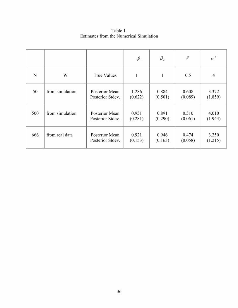
Table 1. Estimates from the Numerical Simulation

1β

2β

ρ

2σ

N

W

True Values

1

1

0.5

4

50

from simulation

Posterior Mean Posterior Stdev.

1.286

(0.622)

0.884

(0.501)

0.608

(0.089)

3.372

(1.859)

500

from simulation

Posterior Mean Posterior Stdev.

0.951

(0.281)

0.891

(0.290)

0.510

(0.061)

4.010

(1.944)

666

from real data

Posterior Mean Posterior Stdev.

0.921

(0.153)

0.946

(0.163)

0.474

(0.058)

3.250

(1.215)

36

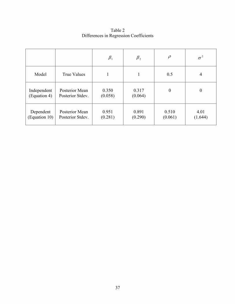
Table 2 Differences in Regression Coefficients

1β

2β

ρ

2σ

Model

True Values

1

1

0.5

4

Independent (Equation 4)

Posterior Mean Posterior Stdev.

0.350

(0.058)

0.317

(0.064)

0

0

Dependent

(Equation 10)

Posterior Mean Posterior Stdev.

0.951

(0.281)

0.891

(0.290)

0.510

(0.061)

4.01

(1.644)

37

Table 3. Sample Statistics

Variable

Mean Standard Deviation

Car Choice (1=Japanese, 0=Non-Japanese) 0.856 0.351 Difference Price (in 100 $s) -2.422 2.998 Difference in Options (in 100 $s) 0.038 0.342 Age of Buyer (in number of years) 48.762 13.856 Annual Income of Buyer (in 1000 $s) 66.906 25.928 Ethnic Origin (1=Asian, 0=Non-Asian) 0.117 0.321 Education (1=College, 0=Below College) 0.349 0.477 Latitude (relative to 30 = original -30) 3.968 0.484 Longitude (relative to –110 = original +110) -8.071 0.503

38

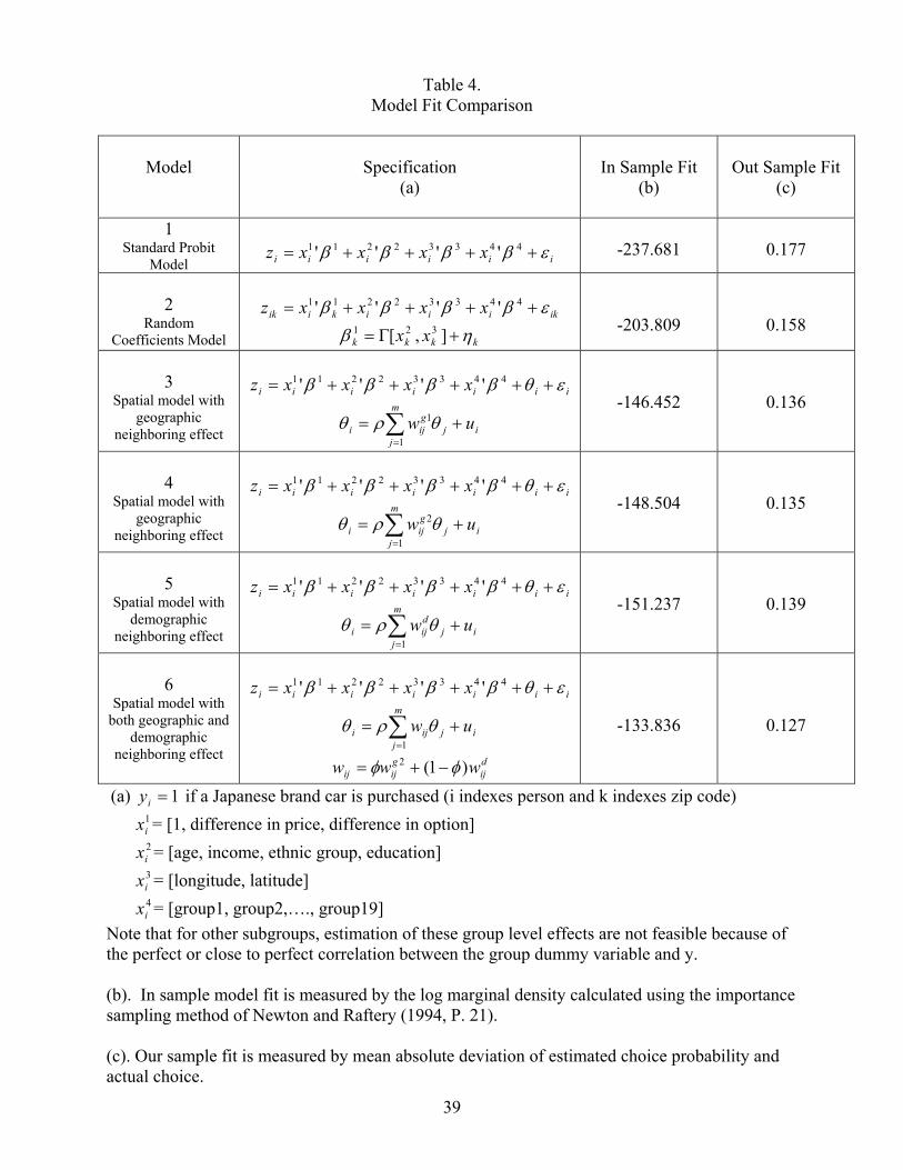
Table 4. Model Fit Comparison

Model

Specification (a)

In Sample Fit

(b)

Out Sample Fit

(c)

1 Standard Probit

Model

iiiiii xxxxz εββββ ++++= 44332211 ''''

-237.681

0.177

2

Random Coefficients Model

ikiiikiik xxxxz εββββ ++++= 44332211 ''''

kkkk xx ηβ +Γ= ],[ 321

-203.809

0.158

3

Spatial model with geographic

neighboring effect

iiiiiii xxxxz εθββββ +++++= 44332211 ''''

i

m

jj

giji uw += ∑

=1

1θρθ

-146.452

0.136

4

Spatial model with geographic

neighboring effect

iiiiiii xxxxz εθββββ +++++= 44332211 ''''

i

m

jj

giji uw += ∑

=1

2θρθ

-148.504

0.135

5

Spatial model with demographic

neighboring effect

iiiiiii xxxxz εθββββ +++++= 44332211 ''''

i

m

jj

diji uw += ∑

=1θρθ

-151.237

0.139

6

Spatial model with both geographic and

demographic neighboring effect

iiiiiii xxxxz εθββββ +++++= 44332211 ''''

i

m

jjiji uw += ∑

=1θρθ

dij

gijij www )1(2 φφ −+=

-133.836

0.127

(a) if a Japanese brand car is purchased (i indexes person and k indexes zip code) 1=iy = [1, difference in price, difference in option] 1

ix = [age, income, ethnic group, education] 2

ix = [longitude, latitude] 3

ix = [group1, group2,…., group19] 4

ixNote that for other subgroups, estimation of these group level effects are not feasible because of the perfect or close to perfect correlation between the group dummy variable and y. (b). In sample model fit is measured by the log marginal density calculated using the importance sampling method of Newton and Raftery (1994, P. 21). (c). Our sample fit is measured by mean absolute deviation of estimated choice probability and actual choice.

39

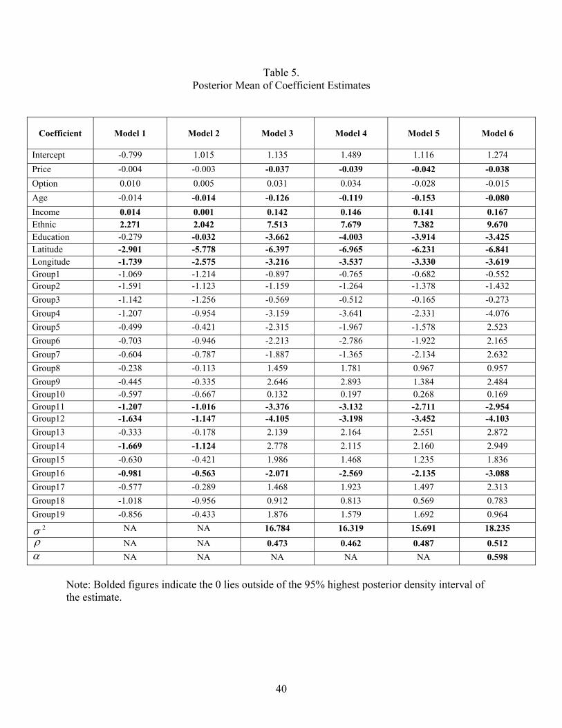
Table 5. Posterior Mean of Coefficient Estimates

Coefficient

Model 1

Model 2

Model 3

Model 4

Model 5

Model 6

Intercept -0.799 1.015 1.135 1.489 1.116 1.274 Price -0.004 -0.003 -0.037 -0.039 -0.042 -0.038 Option 0.010 0.005 0.031 0.034 -0.028 -0.015 Age -0.014 -0.014 -0.126 -0.119 -0.153 -0.080 Income 0.014 0.001 0.142 0.146 0.141 0.167 Ethnic 2.271 2.042 7.513 7.679 7.382 9.670 Education -0.279 -0.032 -3.662 -4.003 -3.914 -3.425 Latitude -2.901 -5.778 -6.397 -6.965 -6.231 -6.841 Longitude -1.739 -2.575 -3.216 -3.537 -3.330 -3.619 Group1 -1.069 -1.214 -0.897 -0.765 -0.682 -0.552 Group2 -1.591 -1.123 -1.159 -1.264 -1.378 -1.432 Group3 -1.142 -1.256 -0.569 -0.512 -0.165 -0.273 Group4 -1.207 -0.954 -3.159 -3.641 -2.331 -4.076 Group5 -0.499 -0.421 -2.315 -1.967 -1.578 2.523 Group6 -0.703 -0.946 -2.213 -2.786 -1.922 2.165 Group7 -0.604 -0.787 -1.887 -1.365 -2.134 2.632 Group8 -0.238 -0.113 1.459 1.781 0.967 0.957 Group9 -0.445 -0.335 2.646 2.893 1.384 2.484 Group10 -0.597 -0.667 0.132 0.197 0.268 0.169 Group11 -1.207 -1.016 -3.376 -3.132 -2.711 -2.954 Group12 -1.634 -1.147 -4.105 -3.198 -3.452 -4.103 Group13 -0.333 -0.178 2.139 2.164 2.551 2.872 Group14 -1.669 -1.124 2.778 2.115 2.160 2.949 Group15 -0.630 -0.421 1.986 1.468 1.235 1.836 Group16 -0.981 -0.563 -2.071 -2.569 -2.135 -3.088 Group17 -0.577 -0.289 1.468 1.923 1.497 2.313 Group18 -1.018 -0.956 0.912 0.813 0.569 0.783 Group19 -0.856 -0.433 1.876 1.579 1.692 0.964

2σ NA NA 16.784 16.319 15.691 18.235 ρ NA NA 0.473 0.462 0.487 0.512 α NA NA NA NA NA 0.598

Note: Bolded figures indicate the 0 lies outside of the 95% highest posterior density interval of the estimate.

40

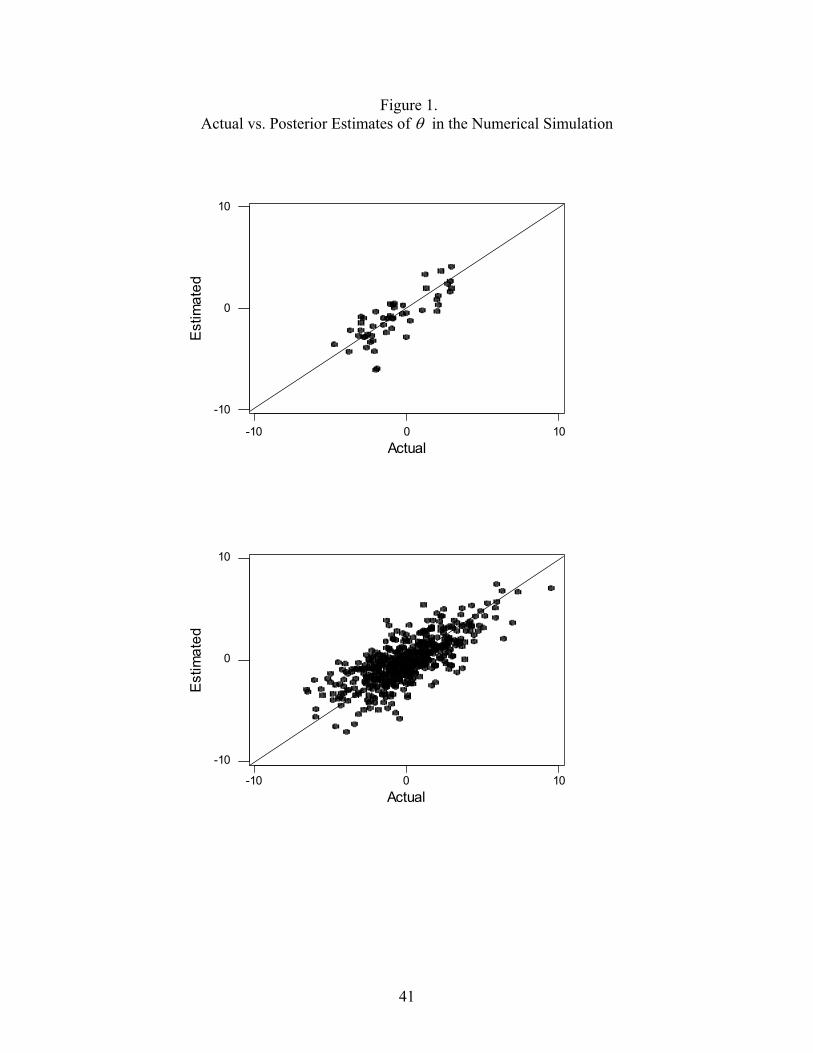
Figure 1. Actual vs. Posterior Estimates of θ in the Numerical Simulation

-10 0 10

-10

0

10

Actual

Estim

ated

-10 0 10

-10

0

10

Actual

Estim

ated

41

6-6

6

-6

Actual

Estim

ated

42

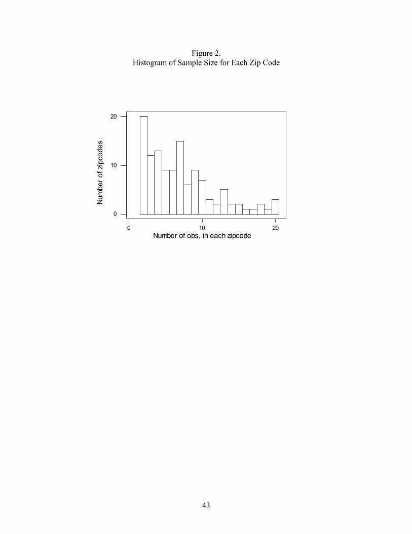
Figure 2. Histogram of Sample Size for Each Zip Code

20100

20

10

0

Number of obs. in each zipcode

Num

ber o

f zip

code

s

43

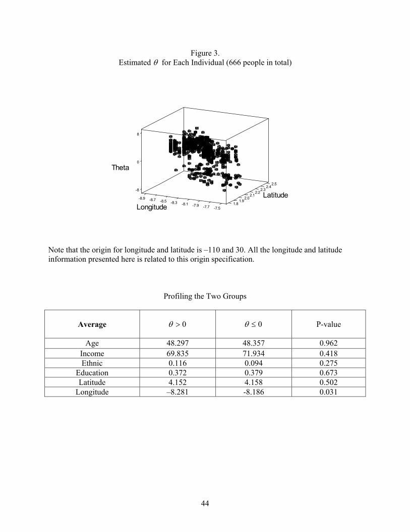
Figure 3. Estimated θ for Each Individual (666 people in total)

2.52.4

2.32.2

-8.9

-8Latitude2.1

-8.7

0

-8.52.0

-8.3

8

-8.11.9

-7.9

Theta

-7.7 -7.51.8Longitude

Note that the origin for longitude and latitude is –110 and 30. All the longitude and latitude information presented here is related to this origin specification.

Profiling the Two Groups

Average

0>θ

0≤θ

P-value

Age 48.297 48.357 0.962 Income 69.835 71.934 0.418 Ethnic 0.116 0.094 0.275

Education 0.372 0.379 0.673 Latitude 4.152 4.158 0.502

Longitude –8.281 -8.186 0.031

44