Modeling Impact Transients Analysis in the Time...

Frequency [Hz]

OriginalLMS

Time [s]

Modeling Impact Transients

Analysis in the Time-DomainMaster of Science Thesis in the Master’s Programme Sound and Vibration

HENRIK GULDBRANSEN

MATTIAS LUNDIN

Department of Civil and Environmental Engineering

Division of Applied Acoustics

Vibroacoustics Group

CHALMERS UNIVERSITY OF TECHNOLOGY

Goteborg, Sweden 2015

Modeling Impact TransientsAnalysis in the Time-Domain

© HENRIK GULDBRANSEN & MATTIAS LUNDIN, 2015

Master’s Thesis 2015:151

Department of Civil and Environmental EngineeringDivision of Applied AcousticsVibroacoustics GroupChalmers University of TechnologySE-41296 GoteborgSweden

Tel. +46-(0)31 772 1000

Reproservice / Department of Civil and Environmental EngineeringGoteborg, Sweden 2015

Modeling Impact TransientsAnalysis in the Time-DomainMaster’s Thesis in the Master’s programme in Sound and Vibration

HENRIK GULDBRANSEN & MATTIAS LUNDINDepartment of Civil and Environmental EngineeringDivision of Applied AcousticsVibroacoustics GroupChalmers University of Technology

Abstract

This thesis has studied whether or not the LMS adaptive algorithm is a favourable wayof estimating the forces acting upon a car when hitting a small obstacle. The study hasmainly been made as a comparison between the LMS algorithm and an IFRF methodusing three different approaches. First approach was a virtual study, comparing howwell the forces were estimated by the two methods. The next step was using impacthammer measurements to determine how well the method could recreate a simpleexcitation. Lastly pressure was measured inside a car compartment while it was beingdriven over an obstacle and the pressure was calculated using each of the methods. Theresults of the first two cases suggests that the LMS is a more favourable approach whenestimating the actual excitation. This was also found in the last case where the energyspectral density of the calculated pressure is estimated fairly well by both methods.In time domain there were larger differences between the estimated forces and themeasurements.

Keywords: Force identification, Impact transient, time-domain, LMS-algorithm.

iii CHALMERS, Master’s Thesis 2015:151

Contents

Abstract iii

Contents iv

Acknowledgements xiii

Notations xv

1. Introduction 1

2. Theory 3

2.1. The Inverse Problem . . . . . . . . . . . . . . . . . . . . . . . . . . . . . . 32.2. Force Identification . . . . . . . . . . . . . . . . . . . . . . . . . . . . . . . 4

2.2.1. Frequency Domain Methods . . . . . . . . . . . . . . . . . . . . . 42.2.2. Single Value Decomposition . . . . . . . . . . . . . . . . . . . . . . 52.2.3. Implementation of IFRF in MATLAB . . . . . . . . . . . . . . . . . 72.2.4. Limitations . . . . . . . . . . . . . . . . . . . . . . . . . . . . . . . 72.2.5. Time Domain Methods . . . . . . . . . . . . . . . . . . . . . . . . . 92.2.6. The LMS-algorithm . . . . . . . . . . . . . . . . . . . . . . . . . . . 92.2.7. About the LMS-algorithm . . . . . . . . . . . . . . . . . . . . . . . 92.2.8. The LMS-algorithm as a Force Identification Method . . . . . . . 112.2.9. Implementation of LMS method in MATLAB . . . . . . . . . . . . 132.2.10. MISO-System . . . . . . . . . . . . . . . . . . . . . . . . . . . . . . 162.2.11. SIMO . . . . . . . . . . . . . . . . . . . . . . . . . . . . . . . . . . . 162.2.12. MIMO . . . . . . . . . . . . . . . . . . . . . . . . . . . . . . . . . . 18

2.3. Short on transients . . . . . . . . . . . . . . . . . . . . . . . . . . . . . . . 192.3.1. Windowing and the ESD . . . . . . . . . . . . . . . . . . . . . . . . 19

2.4. Defining a System of Coordinates . . . . . . . . . . . . . . . . . . . . . . . 212.5. Noise Generation . . . . . . . . . . . . . . . . . . . . . . . . . . . . . . . . 22

2.5.1. Wave Propagation in Tyres . . . . . . . . . . . . . . . . . . . . . . 22

v

3. Measurements 27

3.1. Drum Measurement Setup . . . . . . . . . . . . . . . . . . . . . . . . . . . 273.1.1. List of Equipment . . . . . . . . . . . . . . . . . . . . . . . . . . . . 283.1.2. Notes About the Method . . . . . . . . . . . . . . . . . . . . . . . 293.1.3. Measurement Points . . . . . . . . . . . . . . . . . . . . . . . . . . 29

3.2. Impact Measurements . . . . . . . . . . . . . . . . . . . . . . . . . . . . . 313.2.1. Impact Measurement Setup . . . . . . . . . . . . . . . . . . . . . . 313.2.2. List of Equipment . . . . . . . . . . . . . . . . . . . . . . . . . . . . 323.2.3. Measurements . . . . . . . . . . . . . . . . . . . . . . . . . . . . . 32

4. ”Simulations” 35

4.1. Virtual Simulation . . . . . . . . . . . . . . . . . . . . . . . . . . . . . . . . 354.1.1. Verification of Method . . . . . . . . . . . . . . . . . . . . . . . . . 354.1.2. Comparison with IFRF . . . . . . . . . . . . . . . . . . . . . . . . . 44

4.2. Impact Hammer Simulations . . . . . . . . . . . . . . . . . . . . . . . . . 484.2.1. SIMO Simulation . . . . . . . . . . . . . . . . . . . . . . . . . . . . 484.2.2. MIMO Simulation . . . . . . . . . . . . . . . . . . . . . . . . . . . 50

4.3. MIMO Equivalent Forces . . . . . . . . . . . . . . . . . . . . . . . . . . . . 604.4. Drum Measurement Simulations . . . . . . . . . . . . . . . . . . . . . . . 65

4.4.1. Calculation of Accelerations . . . . . . . . . . . . . . . . . . . . . . 654.4.2. Calculation of Pressure . . . . . . . . . . . . . . . . . . . . . . . . . 694.4.3. Comments On Drum Measurements . . . . . . . . . . . . . . . . . 73

5. Conclusions 77

5.1. Virtual simulations . . . . . . . . . . . . . . . . . . . . . . . . . . . . . . . 775.2. Impact Hammer Simulations . . . . . . . . . . . . . . . . . . . . . . . . . 775.3. Drum simulations . . . . . . . . . . . . . . . . . . . . . . . . . . . . . . . . 78

5.3.1. Accelerations . . . . . . . . . . . . . . . . . . . . . . . . . . . . . . 785.3.2. Pressure . . . . . . . . . . . . . . . . . . . . . . . . . . . . . . . . . 78

5.4. Concluding Remarks . . . . . . . . . . . . . . . . . . . . . . . . . . . . . . 79

References 81

A. Glossary 83

CHALMERS, Master’s Thesis 2015:151 vi

List of Figures

2.1. The direct problem (i) and the inverse problem (ii). . . . . . . . . . . . . . 32.2. Rough outline of the implementation of the IFRF method in MATLAB. For

further explanation of the notations used, see section 2.2.1. . . . . . . . . 82.3. Block diagram of an adaptive controller. . . . . . . . . . . . . . . . . . . . 92.4. Block diagram of a modified controller. . . . . . . . . . . . . . . . . . . . 112.5. Example of the original force and the force recreated by an LMS-algorithm. 122.6. Rough outline of the implementation of the LMS method in MATLAB. . . 152.7. Block diagram of a MISO system. . . . . . . . . . . . . . . . . . . . . . . . 162.8. Block diagram of a MISO system. . . . . . . . . . . . . . . . . . . . . . . . 172.9. Block diagram of a MIMO system. . . . . . . . . . . . . . . . . . . . . . . 182.10. Definitions for the forces and directions. . . . . . . . . . . . . . . . . . . . 212.11. Wave types propagating on a tyre: Bending wave (i), longitudinal wave

(ii) and rotational wave (iii) (Taken from [13]). . . . . . . . . . . . . . . . 222.12. Modal (i) and non-modal (ii) behavior of a tyre. (iii) shows the cavity

resonance of the cavity and ↑ denotes the point of excitation. . . . . . . . 232.13. The four first modes of an unconstrained tire. . . . . . . . . . . . . . . . . 252.14. The four first modes of a tire constrained by a road surface. . . . . . . . . 26

3.1. The setup of the measurements conducted at Volvo PV. . . . . . . . . . . 273.2. Obstacles used in measurements.(i) and (ii) are made out of steel while

(iii) is made out of aluminum . . . . . . . . . . . . . . . . . . . . . . . . . 283.3. Accelerometer positions on the knuckle. The positions of the accelerome-

ters are indicated by (Modified from [19]). . . . . . . . . . . . . . . . . . 303.4. Approximate locations of accelerometers (a1 - a6) and microphone (p)

during measurements. Also marked in the figure is the approximateposition of the excitations (Fxyz). . . . . . . . . . . . . . . . . . . . . . . . . 31

3.5. Picture showing the locations where transfer functions where measuredand in which direction the force was applied. . . . . . . . . . . . . . . . . 33

3.6. Illustrating the cube and from where and in which directions the transferfunctions were measured. . . . . . . . . . . . . . . . . . . . . . . . . . . . 33

4.1. Original signal plotted with the signal with added noise. . . . . . . . . . 36

vii

4.2. Comparing estimated forces, using LMS, with input signal in time domain. 364.3. Comparing estimated moments, using LMS, with input signal in time

domain. . . . . . . . . . . . . . . . . . . . . . . . . . . . . . . . . . . . . . . 374.4. Comparing the spectra of the two methods with the original spectra for

X-direction. . . . . . . . . . . . . . . . . . . . . . . . . . . . . . . . . . . . . 374.5. Comparing the spectra of the two methods with the original spectra for

Y-direction. . . . . . . . . . . . . . . . . . . . . . . . . . . . . . . . . . . . . 384.6. Comparing the spectra of the two methods with the original spectra for

Z-direction. . . . . . . . . . . . . . . . . . . . . . . . . . . . . . . . . . . . . 384.7. Comparing the spectra of the two methods with the original spectra for

moment around X-axis. . . . . . . . . . . . . . . . . . . . . . . . . . . . . . 394.8. Comparing the spectra of the two methods with the original spectra for

moment around Y-axis. . . . . . . . . . . . . . . . . . . . . . . . . . . . . . 394.9. Comparing the spectra of the two methods with the original spectra for

moment around Z-axis. . . . . . . . . . . . . . . . . . . . . . . . . . . . . . 404.10. Comparing the spectra of the two methods with the original spectra for

X-direction when noise is added. . . . . . . . . . . . . . . . . . . . . . . . 404.11. Comparing the spectra of the two methods with the original spectra for

Y-direction when noise is added. . . . . . . . . . . . . . . . . . . . . . . . 414.12. Comparing the spectra of the two methods with the original spectra for

Z-direction when noise is added. . . . . . . . . . . . . . . . . . . . . . . . 414.13. Comparing the spectra of the two methods with the original spectra for

moment around X-axis when noise is added. . . . . . . . . . . . . . . . . 424.14. Comparing the spectra of the two methods with the original spectra for

moment around Y-axis when noise is added. . . . . . . . . . . . . . . . . 424.15. Comparing the spectra of the two methods with the original spectra for

moment around Z-axis when noise is added. . . . . . . . . . . . . . . . . 434.16. Comparing acceleration spectra plus added noise at one acceleration at

X-direction. . . . . . . . . . . . . . . . . . . . . . . . . . . . . . . . . . . . . 434.17. Comparing the spectra of the two methods with the original spectra for

X-direction when noise is added. . . . . . . . . . . . . . . . . . . . . . . . 444.18. Comparing the spectra of the two methods with the original spectra for

Y-direction when noise is added. . . . . . . . . . . . . . . . . . . . . . . . 454.19. Comparing the spectra of the two methods with the original spectra for

Z-direction when noise is added. . . . . . . . . . . . . . . . . . . . . . . . 454.20. Comparing the spectra of the two methods with the original spectra for

moment around X-axis when noise is added. . . . . . . . . . . . . . . . . 464.21. Comparing the spectra of the two methods with the original spectra for

moment around Y-axis when noise is added. . . . . . . . . . . . . . . . . 46

CHALMERS, Master’s Thesis 2015:151 viii

4.22. Comparing the spectra of the two methods with the original spectra formoment around Z-axis when noise is added. . . . . . . . . . . . . . . . . 47

4.23. The measured and calculated pressure in time domain when exciting inY-direction. . . . . . . . . . . . . . . . . . . . . . . . . . . . . . . . . . . . . 48

4.24. The difference between the measured and calculated spectral densitywhen exciting in Y-direction. . . . . . . . . . . . . . . . . . . . . . . . . . . 49

4.25. Showing measured pressure and comparing it to spectra calculated frommeasured and calculated force. Excitation is in the centre of the wheel inY-direction. . . . . . . . . . . . . . . . . . . . . . . . . . . . . . . . . . . . . 49

4.26. Showing the measured force and the calculated force in time domainwhen using an excitation mainly in Z-direction.. . . . . . . . . . . . . . . 50

4.27. Showing the ESD of the calculated Force, IFRF and LMS, and the mea-sured force when using an excitation mainly in Z-direction. . . . . . . . . 51

4.28. Showing the measured pressure spectra and comparing it to the spectracalculated from IFRF and LMS. The force was applied in the Z-direction.. 51

4.29. Showing the dB difference between the calculated pressure for LMS andIFRF when force was applied in Z-direction. . . . . . . . . . . . . . . . . 52

4.30. Showing the two time domain signals for forces in Y and Z direction. . . 524.31. Showing the spectra of the measured pressure and comparing it to the

spectra calculated from IFRF and LMS. The force was applied in an angleat the top corner, with mainly components in Z and Y direction . . . . . 53

4.32. Showing the magnitude of the dB difference between the calculated pres-sure for LMS and IFRF when using an excitation at the top rim, withcomponents mainly in Z and Y.. . . . . . . . . . . . . . . . . . . . . . . . . 53

4.33. Calculated time signals for forces in the X,Y and Z directions when ap-plying a force mainly in X-direction. . . . . . . . . . . . . . . . . . . . . . 54

4.34. Calculated time signals for forces in the X,Y and Z directions when ap-plying a force mainly in Y-direction. . . . . . . . . . . . . . . . . . . . . . 55

4.35. Showing the spectra of the measured pressure and comparing it to spectracalculated from IFRF and LMS when excited applying a force mainly inX-direction.. . . . . . . . . . . . . . . . . . . . . . . . . . . . . . . . . . . . 55

4.36. Showing the spectra of the measured pressure and comparing it to spectracalculated from IFRF and LMS when excited applying a force mainly inY-direction. . . . . . . . . . . . . . . . . . . . . . . . . . . . . . . . . . . . . 56

4.37. Showing the coherence for the different channels and directions used.Top is X-direction, followed by Y and lastly Z. . . . . . . . . . . . . . . . 57

4.38. Calculated time signals when using an excitation divided between thethree directions X,Y and Z. . . . . . . . . . . . . . . . . . . . . . . . . . . . 58

ix CHALMERS, Master’s Thesis 2015:151

4.39. Comparing calculated spectra for LMS and IFRF with the spectra mea-sured when exciting the structure using a force evenly distributed overX,Y and Z direction. . . . . . . . . . . . . . . . . . . . . . . . . . . . . . . . 58

4.40. Showing the magnitude of the dB difference between the calculated pres-sure for LMS and IFRF when using an excitation at an angle distirbutedover X, Y and Z directions. . . . . . . . . . . . . . . . . . . . . . . . . . . . 59

4.41. Comparing the calculated spectra from IFRF and LMS to the measuredspectra. Calculation was carried out using three equivalent forces placedat the cube in the centre of the wheel. . . . . . . . . . . . . . . . . . . . . . 60

4.42. Showing the magnitude of the dB difference between the calculated pres-sure for LMS and IFRF using estimated equivalent forces. Structure wasexcited in Z-direction. . . . . . . . . . . . . . . . . . . . . . . . . . . . . . 61

4.43. Showing the magnitude of the dB difference between the calculated pres-sure for LMS and IFRF using estimated equivalent forces. Structure wasexcited in Y-direction. . . . . . . . . . . . . . . . . . . . . . . . . . . . . . . 61

4.44. Showing the magnitude of the dB difference between the calculated pres-sure for LMS and IFRF estimated equivalent forces. excitation in mainlyZ and Y-direction. . . . . . . . . . . . . . . . . . . . . . . . . . . . . . . . . 62

4.45. Showing a comparison between the spectra of the measured pressure andthe calculated spectras, using an excitation in mainly Y-direction. . . . . 62

4.46. Showing a comparison between the spectra of the measured pressure andthe calculated spectras, using an excitation in mainly Z and Y-direction. 63

4.47. Showing a comparison between the spectra of the measured pressure andthe calculated spectras, using an excitation in mainly Y-direction at thewheel centre (When cube was not attached). . . . . . . . . . . . . . . . . 64

4.48. Showing the magnitude of the dB difference between the calculated pres-sure for LMS and IFRF estimated equivalent forces when excited in Y-direction at the center bolt. . . . . . . . . . . . . . . . . . . . . . . . . . . . 64

4.49. Showing the spectra of the calculated and measured acceleration for thecase with a steel obstacle. Position is at subframe and in X-direction. . . 65

4.50. Showing the spectra of the calculated and measured acceleration for thecase with a aluminum obstacle. Position is at subframe and in X-direction. 66

4.51. Showing the spectra of the calculated and measured acceleration for thecase with a steel obstacle. Position is at subframe and in Z-direction. . . 66

4.52. Showing the spectra of the calculated and measured acceleration for thecase with a aluminum obstacle. Position is at subframe and in Z-direction. 67

4.53. Showing the spectra of the calculated and measured acceleration for thecase with a aluminum obstacle. Position is at body and in X-direction. . 67

CHALMERS, Master’s Thesis 2015:151 x

4.54. Showing the spectra of the calculated and measured acceleration for thecase with a aluminum obstacle. Position is at body and in Z-direction. . 68

4.55. Showing measured pressure and comparing it to spectra calculated fromIFRF- and LMS-forces via NTFs from the spindle (Car driven over obstacle(iii) at 30km/h). . . . . . . . . . . . . . . . . . . . . . . . . . . . . . . . . . 70

4.56. Showing measured pressure and comparing it to spectra calculated fromIFRF- and LMS-forces via NTFs from the spindle (Car driven over obstacle(iii) at 30km/h). . . . . . . . . . . . . . . . . . . . . . . . . . . . . . . . . . 70

4.57. Showing measured pressure and comparing it to spectra calculated fromIFRF- and LMS-forces via NTFs from the spindle (Car driven over obstacle(ii) at 30km/h). . . . . . . . . . . . . . . . . . . . . . . . . . . . . . . . . . 71

4.58. Showing measured pressure and comparing it to spectra calculated fromIFRF- and LMS-forces via NTFs from the spindle (Car driven over obstacle(ii) at 30km/h). . . . . . . . . . . . . . . . . . . . . . . . . . . . . . . . . . 71

4.59. Showing the coherence for the different directions used. . . . . . . . . . . 724.60. Showing measured pressure and comparing it to spectra calculated from

IFRF- and LMS-forces via FRFs to the bushings and NTFs into the car(Car driven over obstacle (iii) at 30km/h). . . . . . . . . . . . . . . . . . . 74

4.61. Showing measured pressure and comparing it to spectra calculated fromIFRF- and LMS-forces via FRFs to the bushings and NTFs into the car(Car driven over obstacle (iii) at 30km/h). . . . . . . . . . . . . . . . . . . 74

4.62. Showing measured pressure and comparing it to spectra calculated fromIFRF- and LMS-forces via FRFs to the bushings and NTFs into the car(Car driven over obstacle (ii) at 30km/h). . . . . . . . . . . . . . . . . . . 75

4.63. Showing measured pressure and comparing it to spectra calculated fromIFRF- and LMS-forces via FRFs to the bushings and NTFs into the car(Car driven over obstacle (ii) at 30km/h). . . . . . . . . . . . . . . . . . . 75

xi CHALMERS, Master’s Thesis 2015:151

Acknowledgements

We would like to thank all involved in making this thesis, and especially, WolfgangKropp at Chalmers University of Technology and Fredrik Bartholdsson, Penka Dinkovaand Robert Nagy at Volvo Car Corporation.

xiii

Notations

Symbols

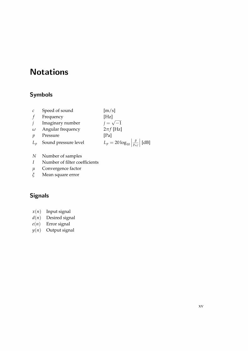
c Speed of sound [m/s]f Frequency [Hz]j Imaginary number j =

√−1

ω Angular frequency 2π f [Hz]p Pressure [Pa]

Lp Sound pressure level Lp = 20 log10

∣∣∣ ppre f

∣∣∣ [dB]

N Number of samplesI Number of filter coefficientsµ Convergence factorξ Mean square error

Signals

x(n) Input signald(n) Desired signale(n) Error signaly(n) Output signal

xv

Abbreviations

NTF Noise transfer functionFFT Fast fourier transformFIR Finite impulse responseFRF Frequency response functionIFRF Inverse frequency response functionLMS Least mean square

CHALMERS, Master’s Thesis 2015:151 xvi

1. Introduction

As fewer model cars are built during the design/evaluation process more extensiveComputer-aided engineering (CAE) is required in order to make better predictions. Oneof the areas that need improvement is the area of impact noise modelling. The aim of thismaster thesis work is to study the possibility of improving VOLVO Car Corporationspossibilities of modelling the noise generated when driving over minor obstacles. Oneof the major problems with this type of modelling is the transient nature of the problemand that it involves forces that for different reasons can’t be measured.

In order to determine the forces one can use what is commonly called inverse forceidentification. The idea is using measured results, such as accelerations and by knowingthe transfer functions of the system one can use these to estimate the excitation forces.Once the forces are known, they can be used in the model to calculate other responses,and see how different changes will impact the end result.

The thesis has looked into two main ideas of force identification, these the first being theinverse frequency response functions, IFRF. And the second is using an LMS adaptivealgorithm.

Initially a virtual study is conducted of the two methods, using known transfer functionsa known force is applied to create a response. From this response the forces are recreatedusing the two methods. This will show how well the two methods estimated theexcitation force as it is known.

The other two studies were of applying a force onto a structure and estimating the impactforce from the actual responses. As this requires accelerations at a number of points onthe hub, measurements were conducted. These were conducted both in a test rig wherethe vehicle were driven over two different obstacles. The second measurements wereconducted with an impact hammer.

Using the results from these measurements, forces were calculated and used to comparethe two methods with the actual measurements. This in order to establish, if possible,which of the two methods is most appropriate for the type of problem.

1

2. Theory

2.1. The Inverse Problem

Lets first assume we have some system, for example a structure, which can be describedby some model. This system is excited in some way which causes a response. We cannow identify two main problems, depending on the variable we seek. The forwardproblem and the inverse problem:

(i) The forward problem means that the system is excited in some way and with thehelp of a model one seeks the response.

(ii) The inverse problem means that the response of the system is known and with thehelp of the model one seeks the unknown excitation acting on the system [5].

This thesis will mainly concern the inverse problem. The two problems are illustratedschematically in figure 2.1. The inverse problem is most often used when it is impossibleto directly measure forces with force transducers. This might due to lack of space orsimply because the force is acting between two structures [6].

ModelExcitation Response

(i)

InverseModel

Excitation Response

(ii)

SoughtSolution

FIGURE 2.1. The direct problem (i) and the inverse problem (ii).

Solutions for the inverse problem has been around for ages, but all comes with its ownset of problems. Many of these problems arise from inverting large matrices in thefrequency domain, which is why many new methods strive to work in the time domaininstead. This thesis aims to investigate one of these methods and its applicability to realworld problems.

3

2.2. Force Identification

The problem of force identification is an extension of the inverse problem outlined insection section 2.1. As the name suggests force identification is an inverse problem wherethe excitation is a force. Usually the measured response is a velocity or an accelerationof some kind. Different methods for force identification exists, and has traditionallybeen carried out in the frequency domain. In recent years however, several researchershave discovered the advantages of a time-domain analysis. The following sections willinvestigate the advantages and disadvantages of some of these methods.

2.2.1. Frequency Domain Methods

Possible frequency domain solutions to the linear system described in section 2.1 isclearly outlined by Stevens in [1], and some of it is recounted in the following. Thesystem can be described in the frequency domain by the equation (2.1):

Hnm(ω)Fm(ω) = Yn(ω) (2.1)

where ω is the angular frequency and Hnm(ω) is the n×m-sized frequency responsematrix:

Hnm(ω) =

H11(ω) H12(ω) . . . H1m(ω)

H21(ω) H22(ω) . . . H2m(ω)...

.... . .

...Hn1(ω) Hn2(ω) . . . Hnm(ω)

(2.2)

Fm(ω) and Yn(ω) is the m-sized vector of exciting forces and the n-sized vector ofresponses, respectively:

Fm(ω) =[

F1(ω) F2(ω) . . . Fm(ω)]T

(2.3)

Yn(ω) =[Y1(ω) Y2(ω) . . . Yn(ω)

]T(2.4)

Hnm(ω) and Yn(ω) is assumed to be known and the problem becomes solving equation(2.1) with respect to Fm(ω).

If Hnm(ω) is square (n = m) and invertible, equation (2.1) can be inverted to obtain asolution in the form of:

CHALMERS, Master’s Thesis 2015:151 4

Fm(ω) = H−1nm(ω)Yn(ω) (2.5)

where Hnm(ω)−1 is the inverse of Hnm(ω). In this case the number of responses is equalto the number of forces. In many cases however, this will not be the true. Instead theamount of forces to be determined will either be larger or smaller than the amount ofmeasured responses. The former case is called under-determined and the latter over-determined. The over-determined system is preferred, since in this case averaging canremove some of the random errors in the system.

The solution to the over- and under-determined cases can be obtained with the so calledMoore-Penrose pseudo inverse, as shown in equation (2.6).

Fest(ω) = H+nm(ω)Yn(ω) (2.6)

If the number of responses is larger than the number of forces there exists more thanone solution. The problem then becomes to choose a force vector that fits to the alreadyknown response vector in some logical manner. There are several ways to do this, oneof them is the least squares method, with which we obtain the solution to the pseudoinverse seen below.

H+nm(ω) = [HT

nm(ω)Hnm(ω)]−1HTnm (2.7)

where HTnm is the hermitian transpose of Hnm. Several other solutions exist, both for

under- and over-determined cases, but since the main focus of the thesis is elsewhere,these will not be investigated further.

2.2.2. Single Value Decomposition

A common inversion method, used by computational software such as MATLAB, useswhat is called single value decomposition. It’s described in for example [18]. It uses thefact that a real m× n matrix A can be decomposed on the form:

A = UΣVT (2.8)

where Σ is a diagonal m× n matrix:

5 CHALMERS, Master’s Thesis 2015:151

Σ = diag(σ1, σ2, . . . , σp

)=

σ1 0 . . . 0 00 σ2 . . . 0 0...

.... . .

......

0 0 . . . σp 0

(2.9)

The entries σp are the singular values of the matrix. U is a m×m orthogonal matrix andV is the transpose of a n× n orthogonal matrix examples of which is shown in equations(2.10) and (2.11), respectively.

U =

u11 . . . u1m...

. . ....

um1 . . . umm

(2.10)

V =

v11 . . . v1n...

. . ....

vn1 . . . vnn

(2.11)

In the case where A is a square an non-singular n× n matrix A can be inverted accordingto:

A−1 =(

UΣVT)−1

= VΣ−1UT (2.12)

where

Σ−1 = diag(

σ−11 , σ−1

2 , . . . , σ−1p

)=

σ−1

1 0 . . . 0 00 σ−1

2 . . . 0 0...

.... . .

......

0 0 . . . σ−1p 0

(2.13)

If A on the other hand is singular or ill-conditioned the inverse of A can be approximatedby computing:

A−1 =(

UΣVT)−1≈ VΣ−1

0 UT (2.14)

where


Σ−10 =

{σ−1

p if σp > t0 if σp < t

(2.15)

Where t is a very small value. In other words the smallest values of Σ−10 is substituted

with zeroes. This somewhat remedies the fact that 1σp→ ∞ for very small values of σp,

the cost is a certain loss of information.

2.2.3. Implementation of IFRF in MATLAB

The implementation of a IFRF method in MATLAB is very straight forward. The basiccalculations are outlined in figure 2.2. Most steps does not warrant any comments, but afew things are worth mentioning about MATLABs built in functions and the consequencesome of the steps have on the final result:

(2) The function pinv is used, which calculates the moore-penrose pseudoinverseusing SVD, mentioned in section 2.2.2. This was confirmed by calculating everystep in the SVD not using built in functions, which yielded the same results.

(4) Several impulses are cut but no windowing is applied according to the theoriesdescribed in section 2.3.

(6) The short durations of the impulses means that quite a bit of zero padding has tobe used in order to get the signal the same length as the FRFs. This gives a spectrathat seems to have a higher resolution than it actually have, since zero paddingdoes not create any new information.

2.2.4. Limitations

The frequency domain method described above, although simple in its execution, comeswith a number of problems. A problem widely discussed in literature is the problemof the matrix-inversion. This problem is ill-conditioned in the sense that small errorsin the matrix pre-inversion might result in large errors after inversion. The primarysources for these small errors are measurement noise and errors that stem from themodeling of the system [1]. Because of the potential of these errors rendering the resultsmeaningless, countless regularization methods, such as Tikhonov regularization, haveemerged throughout the years.


Load FRF→ H(ω)

fs=1600Hz

1

Invert usingpinv→ H−1(ω)

2

Load Acc.fs=8192Hz

3

Cut individual impulses

4

Resample tofs=1600Hz

5

FFT and zero padto length of FRF→ Y(ω)

6

Multiply→F(ω) = H−1(ω)Y(ω)

7

Calculate averageforce of impulses

8

Multiply with NTF

9

Calculate averagepressure of impulses

10

FIGURE 2.2. Rough outline of the implementation of the IFRF method in MATLAB. Forfurther explanation of the notations used, see section 2.2.1.


2.2.5. Time Domain Methods

2.2.6. The LMS-algorithm

The use of the LMS algorithm for force identification was first presented by Kropp andLarson in [7]. The method involves a modification of the LMS-algorithm invented byWidrow and Hoff and which is thoroughly described in for example [2] and [4].

2.2.7. About the LMS-algorithm

Lets first take a look at the LMS-algorithm and how it functions. The purpose of thealgorithm is to minimize the error so that the filter coefficients describes the systemaccurately. An adaptive algorithm is described schematically in figure 2.3, where x(n) isthe input signal, d(n) is the desired signal and y(n) is the output signal.

x(n) e(n)∑

h0

h(n)

d(n)

y(n) −+

FIGURE 2.3. Block diagram of an adaptive controller.

The error signal is the difference between the output signal and the desired signal andcan therefore be written as in equation (2.16).

e(n) = d(n)− y(n) (2.16)

We can write the output signal y(n), as:

y(n) =I−1

∑i=0

hi(n)x(n− i) = hT(n)x(n) (2.17)

where I is the length of the finite impulse response, h(n) is the vector containing thevalues of the impulse response at time step n and the input signal x(n) is the input signalat time step n:


h(n) = [h0(n), h1(n), . . . , hI−1(n)]T (2.18)

x(n) = [x(n), x(n− 1), . . . , x(n− I + 1)]T (2.19)

where T denotes the vector transpose.

The error function 2.16 can, together with 2.17 be rewritten as:

e(n) = d(n)− hT(n)x(n) (2.20)

The LMS function is based on the minimization of the mean square error ξ(n), which isdefined as the statistical expectation of e(n).

ξ(n) = E[e2(n)

](2.21)

= E[(d(n)− hT(n)x(n))2

](2.22)

= E[d2(n)− 2hT(n)x(n)d(n) + hT(n)x(n)xT(n)h(n)

](2.23)

Clear at this point is that ξ(n) is a quadratic function dependent on the filter coefficientsand the input signal. As physical system, it will be concave upward with a singleminimum value. Thus, by moving down the negative gradient the optimal solution canbe obtained [10]. The gradient can be found by differentiating ξ(n) with respect to h(n).We can therefore express the gradient as:

∇ξ(n) =∂ξ(n)∂h(n)

= 2E[

e(n)∂e(n)∂h(n)

]= −2E [e(n)x(n)] (2.24)

From this we can devise an iterative method for updating the filter coefficients accordingto:

h(n + 1) = h(n)− µ∇ξ(n) = h(n) + 2µE [e(n)x(n)] (2.25)

were the coefficient h is updated every time-step n by some amount µ. However, it isstill problematic that the gradient is expressed as the ensemble average. But as shown by[3] the gradient can be estimated by substituting the function in (2.21) with ξ(n) = e2(n)and thus, by differentiating in the same manner as shown before, we get the expression:


h(n + 1) = h(n) + 2µe(n)x(n) (2.26)

This is, for the sake of simplicity, written as:

h(n + 1) = h(n) + αe(n)x(n) (2.27)

where 2µ = α is the convergence factor. The convergence factor controls the stability andthe rate of adaption of the algorithm. It has been suggested that the optimal convergencefactor can be determined by setting the constraints shown in equation (2.28) [7].

0 < α <(

IE[x2(n)

])−1(2.28)

2.2.8. The LMS-algorithm as a Force Identification Method

In order to use the LMS-algorithm for force identification, it needs to be modified slightly.Instead of seeking to model an impulse response, we now seek the input signal, i.e. theforce applied to a certain structure.

h′i e′(n)∑

x′0(n)

x′(n)

d′(n)

y′(n) −+

FIGURE 2.4. Block diagram of a modified controller.

Since convolution is commutative the input vector x(n) and h(n) in equation (2.17) canbe interchanged. Updating equation (2.25), we thus obtain:

x(n + 1) = x(n)− µ∇ξ(n) = x(n) + 2µE [e(n)h(n)] (2.29)

In section 2.2.6 it was shown that the ensemble average could be substituted with theinstantaneous value, and eventually the system would converge towards a minimumvalue. In this case however, this process is problematic. At time n the values of (2.30) areupdated and at time n + 1 the values of (2.31) are updated (and so forth).


x(n) = [x(n), x(n− 1), . . . , x(n− I + 1)]T (2.30)

x(n + 1) = [x(n + 1), x(n), . . . , x(n− I + 2)]T (2.31)

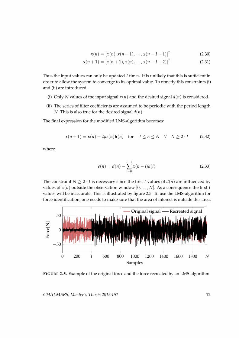
Thus the input values can only be updated I times. It is unlikely that this is sufficient inorder to allow the system to converge to its optimal value. To remedy this constraints (i)and (ii) are introduced:

(i) Only N values of the input signal x(n) and the desired signal d(n) is considered.

(ii) The series of filter coefficients are assumed to be periodic with the period lengthN. This is also true for the desired signal d(n).

The final expression for the modified LMS-algorithm becomes:

x(n + 1) = x(n) + 2µe(n)h(n) for I ≤ n ≤ N ∀ N ≥ 2 · I (2.32)

where

e(n) = d(n)−I−1

∑i=0

x(n− i)h(i) (2.33)

The constraint N ≥ 2 · I is necessary since the first I values of d(n) are influenced byvalues of x(n) outside the observation window [0, . . . , N]. As a consequence the first Ivalues will be inaccurate. This is illustrated by figure 2.5. To use the LMS-algorithm forforce identification, one needs to make sure that the area of interest is outside this area.

.....0.

200.

I.

600.

800.

1000.

1200.

1400.

1600.

1800.

N.

−50

.

0

.

50

.

Samples

.

Forc

e[N

]

.

. ..Original signal . ..Recreated signal

FIGURE 2.5. Example of the original force and the force recreated by an LMS-algorithm.


As in previously described cases, µ need to be under certain constraints in order toensure stability and a sufficient rate of adaptation. The following constraints has beensuggested as suitable:

0 < µ <

(I−1

∑i=0|h(i)|2

)−1

(2.34)

This is the constraint used throughout the work carried out in this thesis, although othersexists.

In order to estimate how well the algorithm has converged and create a stopping criteriafor the algorithm one can set up a relative error according to [7]:

erel =

N

∑i=L+1

e(n)2

N

∑i=L+1

d(n)2

(2.35)

Where N is the total length of the segment studied and L signifies the length of theimpulse response.

2.2.9. Implementation of LMS method in MATLAB

The LMS algorithm can easily be implemented in MATLAB. The basic steps are outlinedin figure 2.6 and further explanations of some of the steps involved are listed below:

(3) How the step size is calculated depends on the type of system investigated. De-pending on the number of responses the step size can be calculated either accordingto equation (2.34) or (2.38).

(4) An in-signal y(n) is calculated for every force and moment taken into account.

(8) An individual error signal e(n) is updated for each force and moment.

(9) Since the force can’t be updated for an infinite time, conditions for terminatingthe iteration process is set. These conditions can either be that the error, e(n),is sufficiently small or that the number of iterations are high enough that noadditional improvement can be expected.

(10) The manner in which the force is updated varies depending on the type of system.For a SISO system the force is updated as described as in section 2.2.8. With several


outputs the force is updated according to equation (2.37), where an average of theresulting error is taken.


Load FRF→ H(ω)

fs=1600Hz

1

Take IFFTH(ω)→ h(n)

2

Calculate step size, α

3

Calculate in-signaly(n) = x(n)h(n)

4

Load Acc. → a(n)fs=8192Hz

5

Resample tofs=1600Hz

6

Cut out the desiredtime period→ d(n)

7

Calculate the errore(n) = d(n)− y(n)

8

Check e(n) and no.of iterations

9

Update force x(n + 1) =x(n) + 2α · e(n)h(n)

10

Calculate averageforce of impulses

11

Multiply with NTF

12

Calculate averagepressure of impulses

13

FIGURE 2.6. Rough outline of the implementation of the LMS method in MATLAB.


2.2.10. MISO-System

When the tyre hits an obstacle, the system will have not one but two points of excitation.And whats more is that at each point the impact force will consist of the forces acting inX,Y and Z direction and the moments acting around each of these axes. This calls for anLMS algorithm which can handle the multiple input - multiple output system, MIMO.We start by using the algorithm for the single input single - output system, SISO. If westudy one point of excitation and one force we will have the system previously shownin figure 2.4.

h′

d′(n)

e′(n)

∑

∑ ∑

x′0,1(n)

x′1(n)

x′2(n)

x′0,2(n)

d′1(n)

y′1(n)++

++

d′2(n)

y′2(n)y′(n) +−

FIGURE 2.7. Block diagram of a MISO system.

If another force is added we will get the system in figure 2.7. The difference in the algo-rithm will be that the two forces both contribute to the response at that position. Whichin turn means that the error calculated is dependent on both these forces, and in orderto calculate the excitation forces, this has to be related to the two forces somehow. Therelation is found in the impulse responses belonging to each force - response path. So inorder to calculate the result one simply has to multiply the error with the correspondingimpulse response and stepsize according to 2.36. The stepsize is calculated like before in2.34.

Fm(n) = Fm(n) + e(n)µmh(i); m = 1, 2; (2.36)

2.2.11. SIMO

From this it is clear that the algorithm is easily adapted to handle multiple input systems.But there is still a need to relate multiple input to multiple output, in order to clarify


how this is done one can continue with studying a system for single input - multipleoutput, SIMO. One such system is shown in figure 2.8.

h′1ih′2i

d′(n)

e′1(n)

e′2(n)

∑

∑

x′0(n)

x′(n)

d′1(n)

y′1(n)

d′2(n)

y′2(n)−

−

+

+

FIGURE 2.8. Block diagram of a MISO system.

The excitation will influence the two response positions, and two separate errors willbe found. Now one needs to relate these errors to the calculation of the excitation force,which will be similar to the process in a SISO system, where the excitation is found byrelating the error to the impulse response and step size. Now however the errors aremultiplied with the corresponding impulse responses and then an average is formed, sowe get the average force exciting this position see equation 2.37.

F(n) = F(n) + µ ·m=M

∑m=1

emhm1M

(2.37)

where M is equal to the total number of response positions. But in order to do thisproperly, the step-size is calculated as an average from the impulse responses accordingto equation 2.38 described by [7].

µ = M

(M

∑m=1

I−1

∑i=0|hm(i)|2

)−1

(2.38)

where M is equal to the total number of response positions and I is the filter length,i.e. the number of samples in the impulse response. h denotes the value of the filtercoefficients at each time sample.


2.2.12. MIMO

With the algorithms for SIMO and MISO ready, an algorithm for a MIMO system can beformed. For each of the exciting forces Fn, there is a response at position m dnm. Linearityis assumed so that the response dm from all forces at response position m, is equal tothe sum of the responses dnm from each of the exciting forces. At each of the responsepositions there will be an error em that is the error between the measured signal ym, andthe calculated response dm.

The block diagram for a 2 input. - 2 output system is shown in figure 2.9, it alreadybecomes a complicated system when illustrating with block diagrams.

h1′

h2′

d′1(n)

e′1(n)

d′2(n)

e′2(n)

∑

∑

∑

∑

x′0,1(n)

x′1(n)

x′2(n)

x′0,2(n)

x′0,2(n)

x′0,1(n)

d′1,1(n)

y′1,1(n)

d′2,1(n)

y′1,2(n)

d′2,2(n)

y′2,2(n)

d′1,2(n)

y′2,1(n)

−

−

+

−

−+

++

++

FIGURE 2.9. Block diagram of a MIMO system.

Using the error signal at all positions, the forces of excitation can be calculated by relatingthe error at the response position, to the impulse response belonging to the excitationposition - response path. This is the correction of the force at time instance n. For aMIMO system this will yield several corrections, and by averaging these and multiplyingwith the step size, the new force estimate at time instance n can be calculated according


to equation 2.37.

Once calculated this procedure is repeated for the next time sample, over the wholeinterval of interest. In order for the algorithm to converge, the process needs to berepeated over the same interval for a number of iterations, this in order to reach aconvergence.

2.3. Short on transients

Before leaving for the section concerning simulations, some short information regardingtransients and the analysis of such will be brought up. A transient signal is as thename suggests transient, that is, it disappears within some given time. The measurableduration of the signal will depend on the system in which it is measured. The amountof damping in the system is one important parameter deciding how long the transientis noticeable. As with any signal, theoretically speaking the energy will remain in thesystem for an infinite time.

But that energy is of no interest since it will neither be measurable nor give rise to anyvibrations or sound. This happens as soon as the levels are beneath the noise floor,another important aspect. In order to observe the transient, it has to be above the noisefloor.

2.3.1. Windowing and the ESD

While studying random or periodic processes it is common to analyse the power spectraldensity, or PSD. The procedure is generally as follows: N consecutive samples of thesignal is chosen. This sequence of the signal usually ends at a discontinuity at theend, and to avoid the effects of leakage a window is applied. After which the FFT istaken over the length of the segment, after which the components of the FFT are scaledaccordingly.

Sxx(n) = Sp|X(n)|2 (2.39)

Gxx(n) =

{Sxx(n) ∗ 2 if n = 1, 2...N/2

Sxx(n) if n = 0(2.40)

Where X(n) is the Fourier transform of the segment, Sxx is the double sided spectra andGxx is the single sided spectra. Sp is a window correction factor that is applied in order


to compensate for the applied window. According to Brandt [17], there are problemsusing the Welch’s estimation described above, especially when dealing with entirelyrandom signals, however as the focus in this thesis is on transient signals, this discussionis not something that will be delved into.

Instead let us consider a transient signal, dealing with impact, it will consist of one ormore peaks and decay after some given time, tdecay. After this time and before the timeof impact there will be the noise floor, if the energy of the transient signal is assumed tobe well above the energy of the noise floor, the levels of the spectral components of thesignal will not be affected much by this noise.

This will in turn mean that there is no need for any windowing, as the leakage will besmall in comparison to the energy in the transient. But it is still important to make surethat at the truncation the levels are, if not zero, very close to zero. While handy, thisposes a problem when analyzing the spectral components.

Due to the limited duration, there will only be a limited number of samples describingthe transient. While one could add an infinite amount of samples to the signal, thefrequency resolution of the signal will not be increased. While it may appear that this isthe case, one is merely interpolating the samples in between the original, low resolutionestimation.

While the PSD is used for periodic or random signals, the ESD, energy spectral density,is used for transient signals. The ESD is similar to the PSD but the main difference is thescaling. The scaling is performed according to Brandt [17] as shown in equations 2.41and 2.42.

Sxx(n) =T

∆ f|X(n)

N|2 = (∆t)2|X(n)|2 (2.41)

Gxx(n) =

{Sxx(n) ∗ 2 if n = 1, 2...N/2

Sxx(n) if n = 0(2.42)

where T signifies the period time, ∆ f is the frequency resolution, ∆t is the time resolutionand N is the amount of samples. Sxx is the double sided spectra and Gxx is the singlesided spectra.

One of the big advantages is of course that zero padding the transient is nothing thatwill alter the spectra, as the energy will be unaffected by such operations.


2.4. Defining a System of Coordinates

Throughout this thesis, when investigating the forces acting upon a tyre a certain systemof coordinates is used. In this system the zero point for each axis is in the absolute centerof the tyre. Assuming a horizontal ground surface, the z-axis is perpendicular to theground plane, the x-axis is parallel to the ground plane and its positive end pointedtowards the driving direction and the y-axis is also parallel to the ground plane butperpendicular to the x- and z-axis. The directions relative to a tyre can be seen in figure2.10.

Fz

Mz

Fx

Mx

Fz

Fy

My

FIGURE 2.10. Definitions for the forces and directions.

From these coordinates we can decompose the forces and moments acting on the tyreinto three distinct forces and three moments [14]:

• Fx - Longitudinal force - The force acting along the x-axis opposite the drivingdirection.

• Fy - Lateral force - The force acting along the y-axis in the direction from the frontright wheel to the left.

• Fz - Normal force - The force acting along the z-axis in the direction from theground plane.

• Mx - Roll moment - The moment about the x-axis.

• My - Pitch moment - The moment about the y-axis.

• Mz - Yaw moment - The moment about the z-axis.

These can then be used to characterize the excitation of the tyre during some process.The definitions of these forces will be the same throughout the thesis, both when lookingat forces acting on tyres and at other points on the car.


2.5. Noise Generation

Mechanisms generating noise from vehicles are abundant, and ranges from friction noiseto aerodynamic noise. In this thesis however, the structural vibrations caused by roaddiscontinuities are of primary importance, therefore the focus is on the noise generationprocesses crucial in that specific case.

2.5.1. Wave Propagation in Tyres

Three kinds of waves can be identified when a tyre is excited: the first wave type isacting as a membrane wave at low frequencies and as a bending wave at slightly higherfrequencies. The second is a longitudinal wave. The third wave type is what is referredto as a rotational wave. This is a wave where the layers of the tyre is moving out ofphase [13]. These waves are illustrated in figure 2.11.

Figure 3. The three wave types considered in the model. Rings represent points in the rubber tread layer andstars represent points in the sti! belt layer.

Figure 4. Dispersion relations for the three wave types represented in the model.** , wave type 1; ) } ) } ) } ) ,wave type 2; } } }} , wave type 3; ........ , Rayleigh waves in rubber.

3.2.2. Dispersion relations for the wave types

Figure 4 shows the dispersion relations for the three waves propagating along thedouble-layer plate without external tension and bedding. The speed of the waves is plottedas a function of frequency for the bending, longitudinal and the in-plane wave.

In the "gure, no membrane e!ect can be seen for the "rst wave type, as expected. Thedispersion relation for the bending waves is proportional to the square root of the frequencyat low frequencies. The speed of the longitudinal waves is constant at low frequencies, but isdecreasing at higher frequencies towards the speed of the surface waves (Rayleigh waves) inthe rubber material, which is also shown in Figure 4. The speed of the in-plane wave (wavetype 3) is very high at the cut-on frequency (about 2500 Hz), but decreases fast to a value

898 K. LARSSON AND W. KROPP

(i)

(ii)

(iii)

FIGURE 2.11. Wave types propagating on a tyre: Bending wave (i), longitudinal wave(ii) and rotational wave (iii) (Taken from [13]).

At certain frequencies there will be constructive interference from waves traveling indifferent directions. This will cause standing wave patterns on the tyre. Circumferentialresonances appear when the circumference of the tyre equals an integer n times thewavelength λ. This modal behavior appears mainly below 500Hz. At higher frequencies,the high damping of the tyre causes waves propagating from the excitation point todecay quickly, thus preventing standing wave patterns [12].

For the purpose of future analysis it is useful to identify the first few modes of thewheel. The exact frequency at which these occur varies from wheel to wheel and from


(i) (ii) (iii)

FIGURE 2.12. Modal (i) and non-modal (ii) behavior of a tyre. (iii) shows the cavityresonance of the cavity and ↑ denotes the point of excitation.

circumstance to circumstance and depending on excitation some modes will not bepresent. Hopefully however, a general behavior can be established. For the sake ofunderstanding, lets look at a unconstrained case first, i.e. where the wheel is freelysuspended and not constrained by the road. The naming convention in the followingtext is taken from [12].

The first few modes are rigid. In other words, there is no deformation of the belt, but thetire vibrates around one of its axes. Four rigid modes can be identified:

(i) The axial mode: The tire vibrates rigidly along the y-axis.

(ii) The torsional mode: The tire vibrates rigidly around the y axis.

(iii) (1,0)-mode: The tire vibrates rigidly in the zx-plane.

(iv) (1,1)-mode: The tire vibrates rigidly around the z-axis in the zx-plane.

These modes differ slightly when constrained by a road surface. The constraint makesthe axial mode ((i)) impossible, and will cause these modes to change. At whats calledthe (1,1) horizontal and (1,1) vertical modes the tire mainly rotates around the y andz-axis, respectively. At the (1,0) horizontal and (1,0) vertical modes the tire mainlyvibrates along the x and z axis, respectively. When the tire is constrained by the road, thetire will show effects of torsional motion around the y axis at the (1,0) horizontal mode .

The frequencies at which these occurs will obviously differ greatly between different carmodels and tires. In [12] the frequencies at which the first constrained modes occur for aparticular model is at 52, 65, 82 and 98 Hz.


2.5.1.1. Cavity Resonance

The structural vibrations on the tyres are also coupled with the pressure inside the tyrecavity. At certain frequencies, just like on the surface of the tyre, constructive interferencewill occur within the tyre cavity, creating standing wave patterns. The very first cavityresonance usually occurs around 200-250Hz for a passenger car tyre. This resonanceis significant for the structural vibrations transmitted into the car. The higher cavityresonances are less significant for transferring vibrations into the car. The very firstresonance can be seen on figure 2.12.

Thomson [15] presented a simplified model for the air cavity in an undeflected tire thatassumes that it can be modeled as a unwrapped torus at low frequencies where thewavelength is much larger than the cross section of the cavity. Also assuming that thecavity is rigid, an estimate of the first cavity resonance can be calculated according to:

fc =cLc

=2c

π(D + d)(2.43)

where c is the speed of sound and Lc is the median length of circumference for the cavity,d is the inner diameter of the cavity and D is outer diameter of the cavity. This methodworks well up to the point were the wavelength becomes the length of the cross-section.

As one wave travel in the rolling direction and another in the opposite direction, thedoppler effect causes this resonance to split into two resonances. In other words thetwo resonances are calculated by putting c = c± cR in equation (2.43), where cR is therolling speed [11].


(i) (ii)

(iii)

Top View

(iv)

FIGURE 2.13. The four first modes of an unconstrained tire.


(v) (vi)

(vii)

Top view

(viii)

FIGURE 2.14. The four first modes of a tire constrained by a road surface.


3. Measurements

Measurements were conducted at Volvo PV in Torslanda, Sweden. The purpose of themeasurements were to investigate the structural response of a car to minor obstacles.

3.1. Drum Measurement Setup

To investigate the response to minor obstacles while avoiding the influence of othernoise sources such as wind noise, road noise, engine noise and so forth, a method usinga laboratory drum facility were used. The facilities used consists of two smooth steeldrums mounted underneath an acoustically isolated floor in a semi anechoic chamber.The drums have diameters of 1.6 meters and are driven by an electric motor locatedunderneath the floor.

Steeldrum

Obstacle

1.6m−x

z

y

FIGURE 3.1. The setup of the measurements conducted at Volvo PV.

During the measurements the front wheels of the car is placed on the steel drum while

27

the the rear wheels are clamped still. The front wheels are driven by the steel drum withthe car engine turned of in order to avoid other influence than that of the tires. A basicsketch of the setup can be seen in figure 3.1.

To investigate the influence of road discontinues, small obstacles were mounted on thesteel drum. The measurements were conducted using obstacles of different shapes andsizes in order to investigate the influence of various excitations. The different obstacles,labeled (i) to (iii), can be seen in figure 3.2. Out of these (i) and (ii) are made out of steelwhile (iii) is made out of aluminum.

To investigate the structural response to different driving speeds, the steel drums weredriven at 1, 5, 10, 15, 20, 25, and 30 km/h. Higher speeds were not possible, because ofthe limited circumference of the drum. At higher speeds the impulses bled into eachother, partly ruining them.

The tires used during the measurement were of the model 275/45R20 manufacturedby Michelin. According to standard notation 275 is the width of the tire, 45 is the ratiobetween the height and the width of the tire expressed in percent, R denotes a radial tireand 20 is the rim diameter in inches [14]. The tire was inflated to a pressure of 2.4 bar.

(i)

16 mm

11.5 mm

(ii)

9 mm

7 mm

(iii)

17 mm

23 mm

FIGURE 3.2. Obstacles used in measurements.(i) and (ii) are made out of steel while (iii)is made out of aluminum

3.1.1. List of Equipment

The following equipment were used during the measurements:

• 12 tri-ax PCB accelerometers model HT356A15 [10mV/g]

• 1 Laptop containing LMS measurement system.

• Scadas Mobile 40 channel front end

• 2 Microphones Bruel & Kjær model 4189-A-021

• Cables


3.1.2. Notes About the Method

Measurements conducted in a lab environment such as described above, will obviouslydiffer somewhat from measurements conducted in a more realistic situation. The primaryadvantage of a laboratory environment is the possibility to repeat the conditions of themeasurements.

An obvious advantage of a drum method is the possibility to exclude most unwantednoise sources such as wind noise and engine noise. Since the surface of the drum isalmost completely flat the influence of road noise can be excluded as well. Therefore,the signal of the obstacle passing underneath the tire can be measured without muchunwanted noise. On the other hand noise from the motor driving the drum mightinfluence the measurements and this needs to be accounted for. It is however unlikelythat this will influence velocity measurements in any significant way.

One disadvantage of mounting obstacles on a steel drum is that the angle of excitationand the pressure distribution on the tire will be slightly different than if mounted on noncurved surface. Part of the procedure involves attaching straps in order to keep the carfrom rolling away, which in turn will alter the actual forces of the impact. As such theforces acting in a tire in a real world situation is therefore expected to differ somewhatfrom the forces acting on the tire driven by the steel drum.

3.1.3. Measurement Points

Measurements were made using accelerometers at a variety of points on the car. Mea-surements of the spindle accelerations were made at four points: Knuc:291, knuc:292,knuc:293 and knuc:294. The positions of these can be seen in figure 3.3. The point onthe knuckle are the ones most referenced throughout the thesis, but measurements weremade at 6 more points. All measurement points are listed in table 3.1.


Knuc:291

Knuc:294 Knuc:293

Knuc:292

FIGURE 3.3. Accelerometer positions on the knuckle. The positions of the accelerometersare indicated by (Modified from [19]).

TABLE 3.1. List of measurements positions used during the measurements.

Positionno.

Positionname

Description

1 Knuc:291 See figure 3.3.2 Knuc:292 See figure 3.3.3 Knuc:293 See figure 3.3.4 Knuc:294 See figure 3.3.5 Body:202 At bushing connecting body and subframe.6 SubF:202 At the subframe close to the bushing.7 Body:241 At the Bushing connecting the top of the front shock ab-

sorbers with the body.8 Strut:241 At the top of the shock absorber.9 Steering

wheelAccelerometer mounted at the very top of the steeringwheel.

10 St:11 Accelerometer mounted beneath the driving seat.


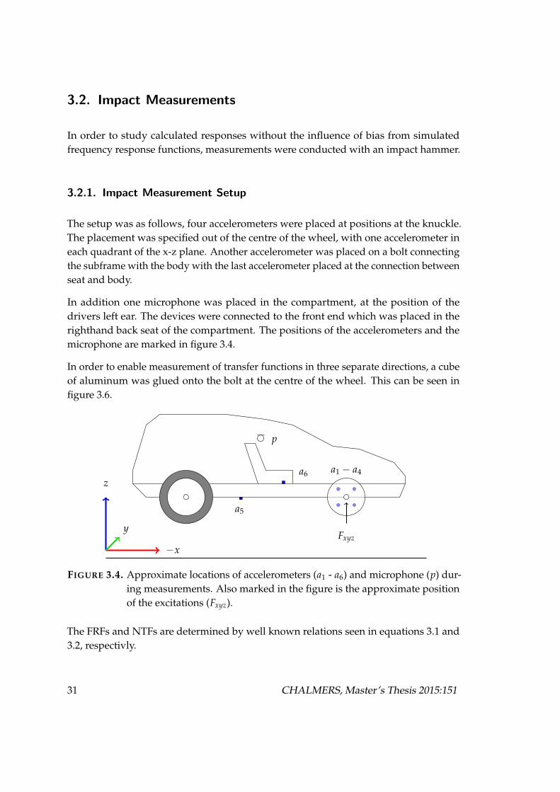
3.2. Impact Measurements

In order to study calculated responses without the influence of bias from simulatedfrequency response functions, measurements were conducted with an impact hammer.

3.2.1. Impact Measurement Setup

The setup was as follows, four accelerometers were placed at positions at the knuckle.The placement was specified out of the centre of the wheel, with one accelerometer ineach quadrant of the x-z plane. Another accelerometer was placed on a bolt connectingthe subframe with the body with the last accelerometer placed at the connection betweenseat and body.

In addition one microphone was placed in the compartment, at the position of thedrivers left ear. The devices were connected to the front end which was placed in therighthand back seat of the compartment. The positions of the accelerometers and themicrophone are marked in figure 3.4.

In order to enable measurement of transfer functions in three separate directions, a cubeof aluminum was glued onto the bolt at the centre of the wheel. This can be seen infigure 3.6.

a1 − a4

Fxyz

p

a5

a6

−x

z

y

FIGURE 3.4. Approximate locations of accelerometers (a1 - a6) and microphone (p) dur-ing measurements. Also marked in the figure is the approximate positionof the excitations (Fxyz).

The FRFs and NTFs are determined by well known relations seen in equations 3.1 and3.2, respectivly.


H(ω) =Yn(ω)

Fn(ω)(3.1)

H(ω) =P(ω)

Fn(ω)(3.2)

where Yn and P are the responses from the accelerometers and the microphone, respec-tively.

3.2.2. List of Equipment

The following equipment were used during the measurements:

• 6 tri-ax DYSTRAN accelerometers model 3023M23 [10mV/g]

• 1 Laptop containing LMS Impact measurement system.

• Scadas Mobile 40 channel front end

• 1 Microphone Bruel & Kjær model 4189-A-021

• 1 Impact Hammer Bruel & Kjær [0.21mV/N]

• Cables

3.2.3. Measurements

Using the impact hammer and tapping the cube, the transfer function for a force actingin X,Y and Z direction was measured. A total of 20 averages was collected for eachdirection. The response was measured with a sampling frequency of 4096 kHz and afrequency resolution of 0.5 Hz.

Once the transfer functions were measured, using the impact hammer, a number ofimpulses and the responses at different positions was measured. The response to aforce in X,Y and Z direction was measured as well as different combinations of thesedirections, e.g. tapping in the corner exciting the different directions somewhat evenlyor at a side with a 45 degree angle.

In addition, due to problems with coherence, measurements of transfer functions wasmeasured at three more positions. One was in the Y direction of the hub centre, withoutthe cube, marked as y2 in figure 3.5. The other two was at the top of the wheel disc, in Yand Z direction, marked as y1 and z1 in figure 3.5. Like previously the impact hammerwas used to create different impulses at the positions.


z1

y1

y2

FIGURE 3.5. Picture showing the locations where transfer functions where measuredand in which direction the force was applied.

z

x

y

FIGURE 3.6. Illustrating the cube and from where and in which directions the transferfunctions were measured.


4. ”Simulations”

Several simulations were conducted over the course of the thesis, starting with verysimple simulations. The first simulations were conducted using known input forces,combining sinusoidals and exponential functions, and using these to create accelerationresponses. These results showed great promise and the work was carried on to analyseresults from actual measurements.

4.1. Virtual Simulation

As an illustration of how the two methods compare, a virtual study will follow. Usingforces estimated from a measurement on the drum with a cleat fastened on the righthand side. In the simulation a total of 3 forces are applied together with 3 moments.Using this excitation accelerations were calculated at 4 tri-axial accelerometer positions.

Then using the same transfer functions and these simulated accelerations, the forceswere calculated using the IFRF method and the LMS algorithm. Two cases are studied,one using the unaltered signal and one using the signal with 5% noise added. Thenoise was estimated from the largest impulse, using 5% of the RMS amplitude andmulltiplying it with a random signal. The modified signal can be seen with the originalsignal in figure 4.1.

4.1.1. Verification of Method

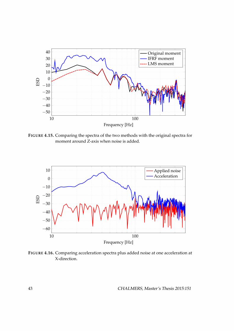
Studying the signal with no noise, it is apparent that the LMS algorithm is very capableof finding the original excitations. The main differences exist in the weaker signals andat some frequencies, and in the moment around Z-axis. It is apparent from the figures 4.2- 4.3, that the estimation in time domain is very accurate. The relative error, calculatedusing equation 2.35, is less than 0.2%. However, studying the spectra in figures 4.4 - 4.9it is apparent that despite this, there are large differences at certain frequencies. This wasfound by M. Sturm et. al [9].

35

2.8 2.9 3 3.1 3.2 3.3−80

−60

−40

−20

0

20

40

Time [s]

Acc

eler

atio

n[m

/s2 ]

Signal with added noiseOriginal signal

FIGURE 4.1. Original signal plotted with the signal with added noise.

5.6 5.8 6 6.2Time [s]

Y-direction

OriginalLMS

5.6 5.8 6 6.2−3,000

−2,000

−1,000

0

1,000

2,000

3,000

Forc

e[N

]

X-direction

OriginalLMS

5.6 5.8 6 6.2

Z-direction

OriginalLMS

FIGURE 4.2. Comparing estimated forces, using LMS, with input signal in time domain.

It is a different situation when applying noise, especially at higher frequencies shownin figures 4.10 - 4.15. However, it is clear that the peaks are identified by the method,and that the overall trend is clearly visible. It is clear studying the results that it is in factthe regions that have the highest power spectral density that are accurately found. Thisis understandable studying the frequency spectra of the noise applied, as the levels at


5.6 5.8 6 6.2Time [s]

Moment around Y-Axis

OriginalLMS

5.6 5.8 6 6.2−300

−200

−100

0

100

200

300

Forc

e[N

]

Moment around X-axis

OriginalLMS

5.6 5.8 6 6.2

Moment around Z-axis

OriginalLMS

FIGURE 4.3. Comparing estimated moments, using LMS, with input signal in timedomain.

10 100

−30

−20

−10

0

10

20

30

40

50

Frequency [Hz]

ESD

Original forceIFRF forceLMS force

FIGURE 4.4. Comparing the spectra of the two methods with the original spectra forX-direction.

higher frequencies are of the same magnitude, see figure 4.16.

In theory however, as the noise should be uncorrelated. And indeed, checking the


10 100

−30

−20

−10

0

10

20

30

40

50

Frequency [Hz]

ESD


FIGURE 4.5. Comparing the spectra of the two methods with the original spectra forY-direction.

10 100

−30

−20

−10

0

10

20

30

40

50

Frequency [Hz]

ESD


FIGURE 4.6. Comparing the spectra of the two methods with the original spectra forZ-direction.

cross-correlation of the noise proves it has very little, close to no correlation. As a resultit should be averaged out. Let us therefore see how the result compares to the IFRFmethod.


10 100−50

−40

−30

−20

−100

10

20

30

40

Frequency [Hz]

ESD

Original momentIFRF momentLMS moment

FIGURE 4.7. Comparing the spectra of the two methods with the original spectra formoment around X-axis.

10 100−50

−40

−30

−20

−100

10

20

30

40

Frequency [Hz]

ESD


FIGURE 4.8. Comparing the spectra of the two methods with the original spectra formoment around Y-axis.


10 100−50

−40

−30

−20

−100

10

20

30

40

Frequency [Hz]

ESD


FIGURE 4.9. Comparing the spectra of the two methods with the original spectra formoment around Z-axis.

10 100

−30

−20

−10

0

10

20

30

40

50

Frequency [Hz]

ESD


FIGURE 4.10. Comparing the spectra of the two methods with the original spectra forX-direction when noise is added.


10 100

−30

−20

−10

0

10

20

30

40

50

Frequency [Hz]

ESD


FIGURE 4.11. Comparing the spectra of the two methods with the original spectra forY-direction when noise is added.

10 100

−30

−20

−10

0

10

20

30

40

50

Frequency [Hz]

ESD


FIGURE 4.12. Comparing the spectra of the two methods with the original spectra forZ-direction when noise is added.


10 100−50

−40

−30

−20

−100

10

20

30

40

Frequency [Hz]

ESD


FIGURE 4.13. Comparing the spectra of the two methods with the original spectra formoment around X-axis when noise is added.

10 100−50

−40

−30

−20

−100

10

20

30

40

Frequency [Hz]

ESD


FIGURE 4.14. Comparing the spectra of the two methods with the original spectra formoment around Y-axis when noise is added.


10 100−50

−40

−30

−20

−100

10

20

30

40

Frequency [Hz]

ESD


FIGURE 4.15. Comparing the spectra of the two methods with the original spectra formoment around Z-axis when noise is added.

10 100

−60

−50

−40

−30

−20

−10

0

10

Frequency [Hz]

ESD

Applied noiseAcceleration

FIGURE 4.16. Comparing acceleration spectra plus added noise at one acceleration atX-direction.


4.1.2. Comparison with IFRF

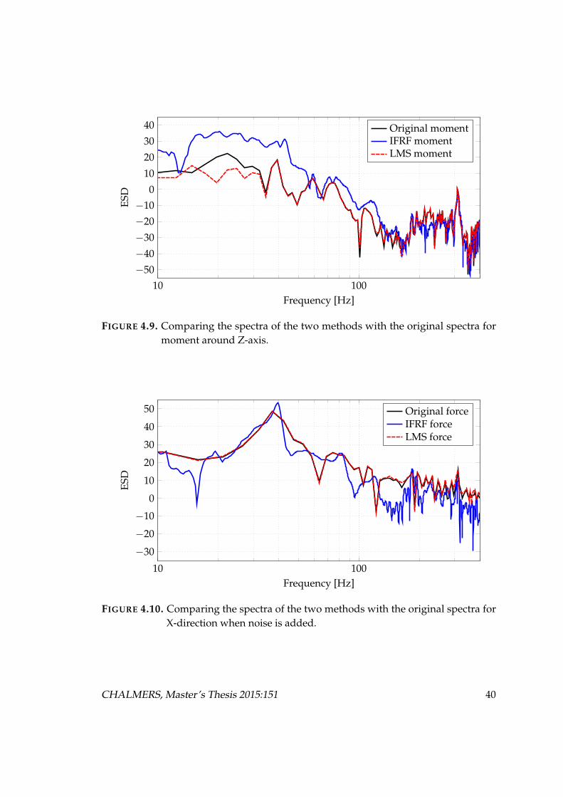
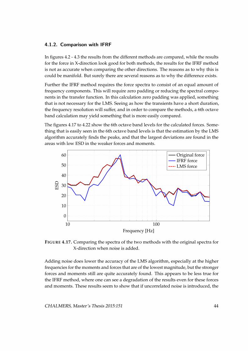
In figures 4.2 - 4.3 the results from the different methods are compared, while the resultsfor the force in X-direction look good for both methods, the results for the IFRF methodis not as accurate when comparing the other directions. The reasons as to why this iscould be manifold. But surely there are several reasons as to why the difference exists.

Further the IFRF method requires the force spectra to consist of an equal amount offrequency components. This will require zero padding or reducing the spectral compo-nents in the transfer function. In this calculation zero padding was applied, somethingthat is not necessary for the LMS. Seeing as how the transients have a short duration,the frequency resolution will suffer, and in order to compare the methods, a 6th octaveband calculation may yield something that is more easily compared.

The figures 4.17 to 4.22 show the 6th octave band levels for the calculated forces. Some-thing that is easily seen in the 6th octave band levels is that the estimation by the LMSalgorithm accurately finds the peaks, and that the largest deviations are found in theareas with low ESD in the weaker forces and moments.

10 100

0

10

20

30

40

50

60

Frequency [Hz]

ESD


FIGURE 4.17. Comparing the spectra of the two methods with the original spectra forX-direction when noise is added.

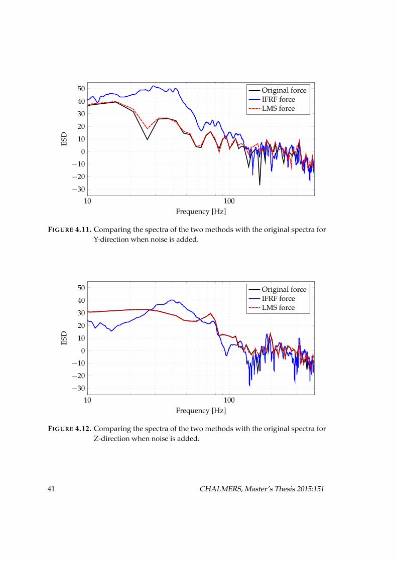
Adding noise does lower the accuracy of the LMS algorithm, especially at the higherfrequencies for the moments and forces that are of the lowest magnitude, but the strongerforces and moments still are quite accurately found. This appears to be less true forthe IFRF method, where one can see a degradation of the results even for these forcesand moments. These results seem to show that if uncorrelated noise is introduced, the


10 100

0

10

20

30

40

50

60

Frequency [Hz]

ESD


FIGURE 4.18. Comparing the spectra of the two methods with the original spectra forY-direction when noise is added.

10 100

0

10

20

30

40

50

60

Frequency [Hz]

ESD


FIGURE 4.19. Comparing the spectra of the two methods with the original spectra forZ-direction when noise is added.

method handles this rather well.


10 100

−20

−10

0

10

20

30

40

Frequency [Hz]

ESD


FIGURE 4.20. Comparing the spectra of the two methods with the original spectra formoment around X-axis when noise is added.

10 100

−20

−10

0

10

20

30

40

Frequency [Hz]

ESD


FIGURE 4.21. Comparing the spectra of the two methods with the original spectra formoment around Y-axis when noise is added.


10 100

−20

−10

0

10

20

30

40

Frequency [Hz]

ESD


FIGURE 4.22. Comparing the spectra of the two methods with the original spectra formoment around Z-axis when noise is added.


4.2. Impact Hammer Simulations

Using the results from the measurements conducted with the impact hammer, resultshave been procured using both IFRF and the LMS algorithm. The results will be dis-played for each of the measurement cases that was described in section 3.

4.2.1. SIMO Simulation

The first results come from a simple excitation in Y-direction, assuming that there isjust one force acting upon the structure. As can be seen from studying the pressure infigure 4.23 there is an underestimation in comparison to the measured pressure. Thiscan be seen in the frequency domain as well. The difference between the measured andcalculated spectral density are shown in figure 4.24.

0 0.05 0.1 0.15 0.2 0.25 0.3 0.35 0.4 0.45 0.5−0.5

−0.25

0

0.25

0.5

0.75

1

Time [s]

Pres

sure

[Pa]

MeasuredCalculated

FIGURE 4.23. The measured and calculated pressure in time domain when exciting inY-direction.

One important aspect is that the measured force is in fact measured, and a lack of timeresolution and sensitivity may influence the measurement. This can be seen if one usesthe measured force to calculate the sound pressure at the microphone, seen in figure4.25. While some of it may be due to background noise, after all the levels in the mic arelow. Even if adding the spectra of the background noise, the levels are lower.

But one can use the measured force and compare the pressure it creates, to the pressuregained from the estimated force, the results are indeed very similar, though the under


0 50 100 150 200 250 300 350 400 450 500−10

−7.5

−5

−2.5

0

2.5

5

7.5

10

Frequency [Hz]

Diff

eren

cein

ESD

FIGURE 4.24. The difference between the measured and calculated spectral densitywhen exciting in Y-direction.

0 100 200 300 400 500 600

−120

−110

−100

−90

−80

−70

Frequency [Hz]

ESD

Measured PressureCalculated force→ PressureMeasured force→ Pressure

FIGURE 4.25. Showing measured pressure and comparing it to spectra calculated frommeasured and calculated force. Excitation is in the centre of the wheel inY-direction.

estimation is still visible.


4.2.2. MIMO Simulation

When the exciting force is at an angle to the rim, the excitation can be split into twoforces, one in Z-direction and one in Y-direction. Using the impulse responses for thesetwo directions, at positions close to the excitation, the force can be estimated. This willof course not be entirely accurate, as the transfer functions will be somewhat differentfrom the ones at the excitation position, but it should be sufficiently similar. Somethingthat the results that will follow seems to suggest.

4.2.2.1. Results From Two Impact Forces

When exciting the structure in one direction, this time in Z direction, the results areobtained shown in figure 4.26. The force is accurately estimated, and whats more, thealgorithm identifies the Z direction as the point of excitation. Looking at the frequencyspectra of the impact, figure 4.27 the results are very good indeed. With levels within 1dB for large parts of the spectra.

0 0.002 0.004 0.006 0.008 0.01−1,000

0

1,000

2,000

3,000

4,000

Time [s]

Forc

e[N

]

CalculatedMeasured

FIGURE 4.26. Showing the measured force and the calculated force in time domainwhen using an excitation mainly in Z-direction..

But as previously mentioned, the measured force is not necessarily completely accurate,and therefore the measured pressure is important to compare. Shown in figure 4.28the calculated spectra very closely resembles the measured, at many of the frequencieswithin 0.5 dB of the measured spectra. Using the IFRF to do the same estimation yields


0 50 100 150 200 250 300 350 400 450 5002

2.5

3

3.5

4

4.5

5

Frequency [Hz]

ESD

MeasuredIFRFLMS

FIGURE 4.27. Showing the ESD of the calculated Force, IFRF and LMS, and the mea-sured force when using an excitation mainly in Z-direction.

similar results, and in order to really study the differences the dB difference is shown infigure 4.29.

0 50 100 150 200 250 300 350 400 450 500

−100

−90

−80

−70

−60

−50

−40

Frequency [Hz]

ESD

MeasuredIFRFLMS

FIGURE 4.28. Showing the measured pressure spectra and comparing it to the spectracalculated from IFRF and LMS. The force was applied in the Z-direction..

Interestingly, the results does not differ much from the IFRF and the LMS, though there


0 50 100 150 200 250 300 350 400 450 5000

5

10

15

20

25

30

35

40

Frequency [Hz]

Mea

sure

d/C

alcu

late

dES

D[d

B] IFRFLMS

FIGURE 4.29. Showing the dB difference between the calculated pressure for LMS andIFRF when force was applied in Z-direction.

are some frequencies where both the IFRF and LMS loses accuracy. Though the LMSonly really loses accuracy at the larger dips, whereas the IFRF seem to lose accuracy atfrequencies of higher magnitudes. But overall, both methods produce good results.

If the excitation is instead at the rim, at an angle, the forces are of a more equal magni-tude, figure 4.30. Assuming that the measured force could be flawed, the best way ofmeasuring the results is comparing with the microphone pressure.

FIGURE 4.30. Showing the two time domain signals for forces in Y and Z direction.

In figure 4.31 the ESD for the microphone pressure is compared. Both methods producegood results, however as shown in figure 4.32, the LMS have frequency ranges where


the estimation is better.

0 50 100 150 200 250 300 350 400 450 500

−110

−100

−90

−80

−70

−60

−50

−40

Frequency [Hz]

ESD

MeasuredIFRFLMS

FIGURE 4.31. Showing the spectra of the measured pressure and comparing it to thespectra calculated from IFRF and LMS. The force was applied in an angleat the top corner, with mainly components in Z and Y direction

0 50 100 150 200 250 300 350 400 450 5000

5

10

15

20

25

30

35

40

45

50

Frequency [Hz]

Mea

sure

d/C

alcu

late

dES

D[d

B] IFRFLMS

;

FIGURE 4.32. Showing the magnitude of the dB difference between the calculated pres-sure for LMS and IFRF when using an excitation at the top rim, withcomponents mainly in Z and Y..


4.2.2.2. Results From Three Impact Forces

The next application of the algorithm is applying it to the case when an aluminum cubeis placed at the wheel hub. Like previously the simulation can be conducted for anexcitation mainly in one direction, and the results are shown in figures 4.33 - 4.34. Likebefore the algorithms identifies mainly a force in the excitation direction.

0 0.01 0.02 0.03Time [s]

Y-direction

IFRFLMS

0 0.01 0.02 0.03−50

0

50

100

150

200

250

300

Forc

e[N

]

X-direction

IFRFLMS

0 0.01 0.02 0.03

Z-direction

IFRFLMS

FIGURE 4.33. Calculated time signals for forces in the X,Y and Z directions when apply-ing a force mainly in X-direction.

Studying the spectra of the estimated pressure one clearly note one thing, figures 4.35-4.36, the worst estimation is at frequencies where there is little power. This is notsurprising, considering that this was the case found in the virtual study as well. But likebefore, if using the measured force to estimate the pressure, there is similar accuracy.This could suggest that the problem is with the measured transfer functions more thananything.

What is more, the IFRF is showing larger differences at frequencies compared to theLMS. If comparing to previous results, they no longer follow the same trends.

Studying the coherence, this does not seem unlikely, it is low over large portions of thefrequency range, see figure 4.37. And this is only for the pressure, the situation is similarfor the transfer functions measured to the accelerometers.

Using an excitation at one corner yield three forces in the same order of magnitude, seefigure 4.38. From these forces the pressure at the mic is as before close to the measured,


0 0.2 0.4−100

0

100

200

300

400

500

Time[s]

Y-direction

IFRFLMS

0 0.2 0.4−50

0

50

100

150

200

Forc

e[N

]X-direction

IFRFLMS

0 0.2 0.4−40

−30

−20

−10

0

10

20

Z-direction

IFRFLMS

FIGURE 4.34. Calculated time signals for forces in the X,Y and Z directions when apply-ing a force mainly in Y-direction.

0 50 100 150 200 250 300 350 400 450 500 550 600

−110

−100

−90

−80

−70

−60

−50

−40

Frequency [Hz]

ESD

MeasuredIFRFLMS

FIGURE 4.35. Showing the spectra of the measured pressure and comparing it to spectracalculated from IFRF and LMS when excited applying a force mainly inX-direction..

figure 4.39 and 4.40.


0 50 100 150 200 250 300 350 400 450 500 550 600

−110

−100

−90

−80

−70

−60

−50

−40

Frequency [Hz]

ESD

MeasuredIFRFLMS

FIGURE 4.36. Showing the spectra of the measured pressure and comparing it to spectracalculated from IFRF and LMS when excited applying a force mainly inY-direction.


00.20.40.60.8

1

Coh

eren

ce

00.20.40.60.8

1

Coh

eren

ce

0 100 200 300 400 5000

0.20.40.60.8

1

Frequency [Hz]

Coh

eren

ce

FIGURE 4.37. Showing the coherence for the different channels and directions used. Topis X-direction, followed by Y and lastly Z.


0 0.2 0.4Time[s]

Y-direction

IFRFLMS

0 0.2 0.4−50

0

50

100

150Fo

rce[

N]

X-direction

IFRFLMS

0 0.2 0.4

Z-direction

IFRFLMS

FIGURE 4.38. Calculated time signals when using an excitation divided between thethree directions X,Y and Z.

0 50 100 150 200 250 300 350 400 450 500 550

−110

−100

−90

−80

−70

−60

−50

−40

−30

Frequency [Hz]

ESD

MeasuredIFRFLMS

FIGURE 4.39. Comparing calculated spectra for LMS and IFRF with the spectra mea-sured when exciting the structure using a force evenly distributed overX,Y and Z direction.


0 50 100 150 200 250 300 350 400 4500

5

10

15

20

25

30

35

Frequency [Hz]

Mea

sure

d/C

alcu

late

dES

D[d

B] IFRFLMS

FIGURE 4.40. Showing the magnitude of the dB difference between the calculated pres-sure for LMS and IFRF when using an excitation at an angle distirbutedover X, Y and Z directions.


4.3. MIMO Equivalent Forces

The idea in this section is that if the transfer functions from a position, different to theexcitation position, to all the measurement positions is known, one can calculate theforces at this position which will yield the same excitation. Taking this one step further,one can calculate the response at other positions using these calculated forces as long asthe transfer function is known.

More interesting results come from using the transfer functions measured using the cubeto create forces yielding equivalent accelerations at the measurement positions. The firstcase studied is using the excitation in Z-direction at the top of the wheel. Then usingthe measured accelerations to calculate excitation forces at the hub, one gets the resultsshown in figure 4.41. Interestingly, if comparing to some of the previous results, there isa difference between the two methods, while the LMS is at large better at estimation, seefigure 4.42.

0 50 100 150 200 250 300 350 400 450 500

−110

−100

−90

−80

−70

−60

−50

−40

−30

Frequency [Hz]

ESD

MeasuredIFRFLMS

FIGURE 4.41. Comparing the calculated spectra from IFRF and LMS to the measuredspectra. Calculation was carried out using three equivalent forces placedat the cube in the centre of the wheel.

The results differ some when using excitation in either ZY or Y direction at the top ofthe wheel. There are different frequency regions that are better estimated by differentmethods. Something that is easily seen in figures 4.43 and 4.44.

This is interesting and also studying the spectra shows some interesting details, figures4.45 and 4.46. The spectra no longer only differ in mostly magnitude, but in some


0 50 100 150 200 250 300 350 400 450 50005

1015202530354045505560

Frequency [Hz]

Cal

cula

ted/

Mea

sure

dES

D[d

B] IFRFLMS

FIGURE 4.42. Showing the magnitude of the dB difference between the calculated pres-sure for LMS and IFRF using estimated equivalent forces. Structure wasexcited in Z-direction.

0 50 100 150 200 250 300 350 400 450 50005

1015202530354045505560

Frequency [Hz]

Mea

sure

d/C

alcu

late

dES

D[d

B] IFRFLMS

FIGURE 4.43. Showing the magnitude of the dB difference between the calculated pres-sure for LMS and IFRF using estimated equivalent forces. Structure wasexcited in Y-direction.

frequency regions the overall shape of the spectra is different. Which gives some clues


0 50 100 150 200 250 300 350 400 450 500 550 6000

10

20

30

40

50

60

Frequency [Hz]

Cal

cula

ted/

Mea

sure

dES

D[d

B] IFRFLMS

FIGURE 4.44. Showing the magnitude of the dB difference between the calculated pres-sure for LMS and IFRF estimated equivalent forces. excitation in mainlyZ and Y-direction.

as to what is in fact happening. But before speculating let us also study the excitation atthe centre of the wheel using equivalent forces.

0 50 100 150 200 250 300 350 400 450 500 550 600

−110

−100

−90

−80

−70

−60

−50

−40

−30

Frequency [Hz]

ESD

MeasuredIFRFLMS

FIGURE 4.45. Showing a comparison between the spectra of the measured pressure andthe calculated spectras, using an excitation in mainly Y-direction.


0 50 100 150 200 250 300 350 400 450 500 550 600

−110

−100

−90

−80

−70

−60

−50

−40

−30

Frequency [Hz]

ESD

MeasuredIFRFLMS

FIGURE 4.46. Showing a comparison between the spectra of the measured pressure andthe calculated spectras, using an excitation in mainly Z and Y-direction.

The last results show the calculated pressure using an excitation at the center bolt of thestructure in Y. From this excitation equivalent forces are calculated and from these theresulting pressure is estimated. Once again the LMS shows a better estimation for thelarger part of the spectra, see figure 4.47 and 4.48.


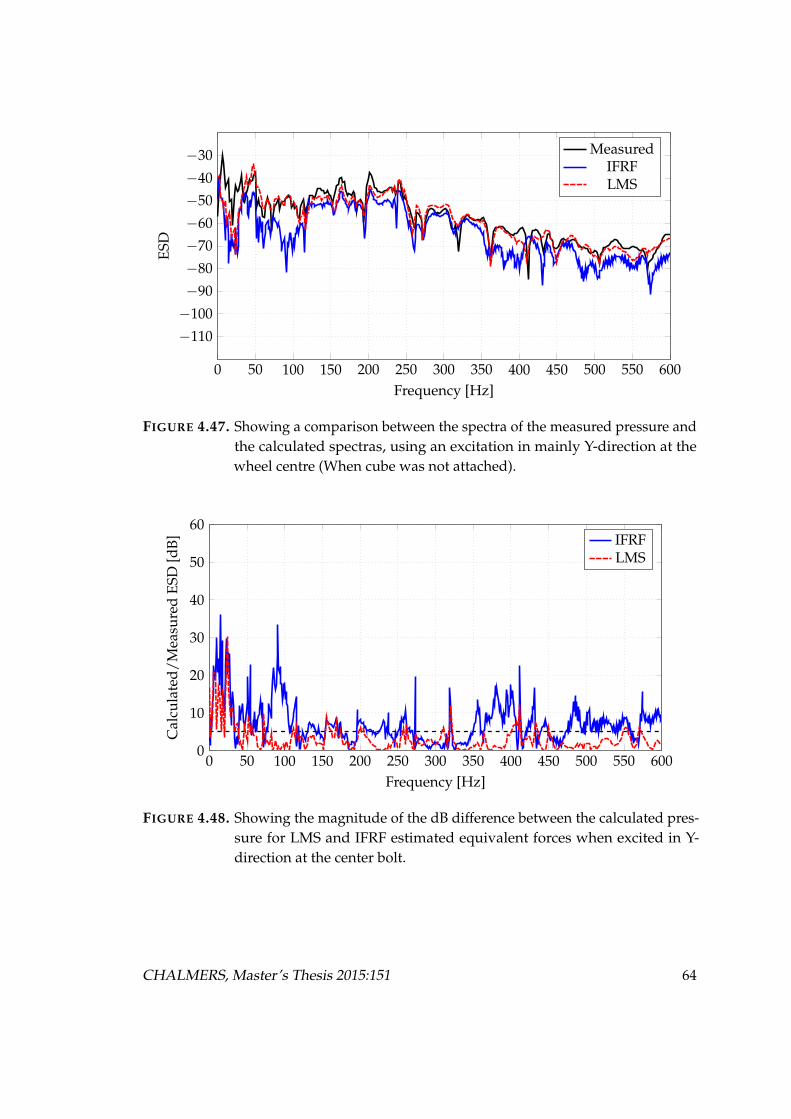
0 50 100 150 200 250 300 350 400 450 500 550 600

−110

−100

−90

−80

−70

−60

−50

−40

−30

Frequency [Hz]

ESD

MeasuredIFRFLMS

FIGURE 4.47. Showing a comparison between the spectra of the measured pressure andthe calculated spectras, using an excitation in mainly Y-direction at thewheel centre (When cube was not attached).

0 50 100 150 200 250 300 350 400 450 500 550 6000

10

20

30

40

50

60

Frequency [Hz]

Cal

cula

ted/

Mea

sure

dES

D[d

B] IFRFLMS

FIGURE 4.48. Showing the magnitude of the dB difference between the calculated pres-sure for LMS and IFRF estimated equivalent forces when excited in Y-direction at the center bolt.


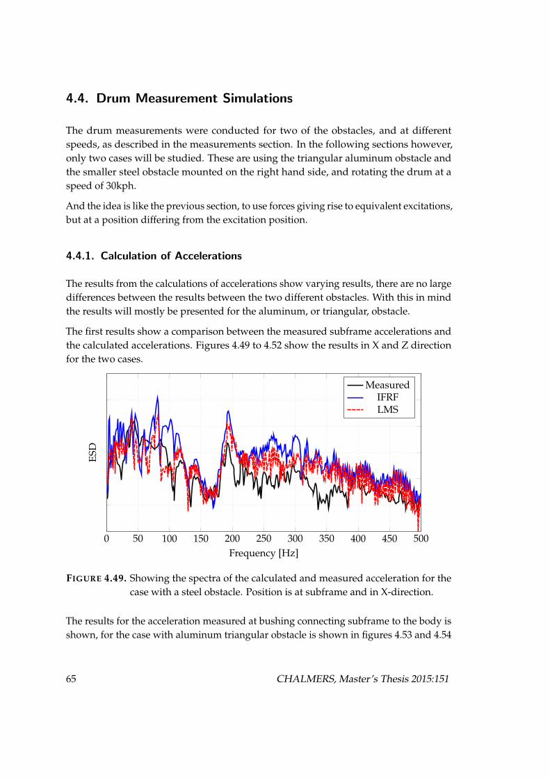
4.4. Drum Measurement Simulations

The drum measurements were conducted for two of the obstacles, and at differentspeeds, as described in the measurements section. In the following sections however,only two cases will be studied. These are using the triangular aluminum obstacle andthe smaller steel obstacle mounted on the right hand side, and rotating the drum at aspeed of 30kph.

And the idea is like the previous section, to use forces giving rise to equivalent excitations,but at a position differing from the excitation position.

4.4.1. Calculation of Accelerations

The results from the calculations of accelerations show varying results, there are no largedifferences between the results between the two different obstacles. With this in mindthe results will mostly be presented for the aluminum, or triangular, obstacle.

The first results show a comparison between the measured subframe accelerations andthe calculated accelerations. Figures 4.49 to 4.52 show the results in X and Z directionfor the two cases.

0 50 100 150 200 250 300 350 400 450 500Frequency [Hz]

ESD

MeasuredIFRFLMS

FIGURE 4.49. Showing the spectra of the calculated and measured acceleration for thecase with a steel obstacle. Position is at subframe and in X-direction.

The results for the acceleration measured at bushing connecting subframe to the body isshown, for the case with aluminum triangular obstacle is shown in figures 4.53 and 4.54


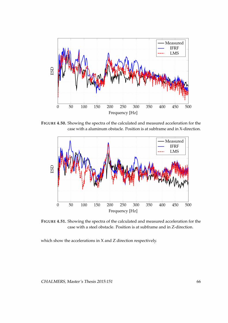
0 50 100 150 200 250 300 350 400 450 500Frequency [Hz]

ESD

MeasuredIFRFLMS

FIGURE 4.50. Showing the spectra of the calculated and measured acceleration for thecase with a aluminum obstacle. Position is at subframe and in X-direction.

0 50 100 150 200 250 300 350 400 450 500Frequency [Hz]

ESD

MeasuredIFRFLMS

FIGURE 4.51. Showing the spectra of the calculated and measured acceleration for thecase with a steel obstacle. Position is at subframe and in Z-direction.

which show the accelerations in X and Z direction respectively.


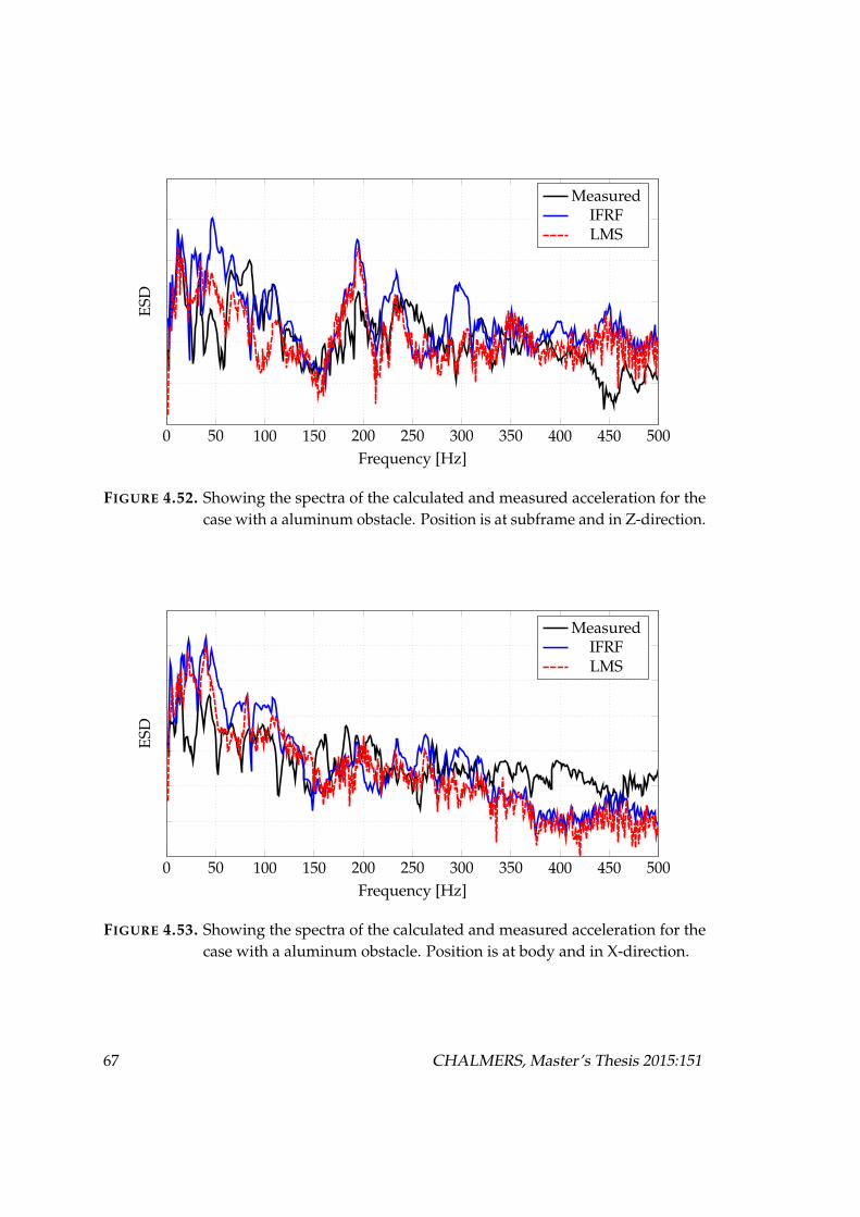
0 50 100 150 200 250 300 350 400 450 500Frequency [Hz]

ESD

MeasuredIFRFLMS

FIGURE 4.52. Showing the spectra of the calculated and measured acceleration for thecase with a aluminum obstacle. Position is at subframe and in Z-direction.

0 50 100 150 200 250 300 350 400 450 500Frequency [Hz]

ESD

MeasuredIFRFLMS

FIGURE 4.53. Showing the spectra of the calculated and measured acceleration for thecase with a aluminum obstacle. Position is at body and in X-direction.


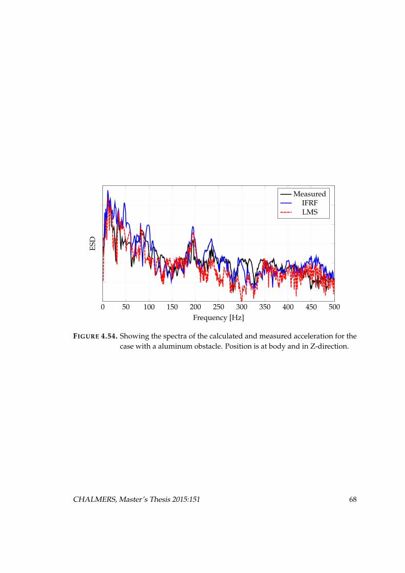
0 50 100 150 200 250 300 350 400 450 500Frequency [Hz]

ESD

MeasuredIFRFLMS

FIGURE 4.54. Showing the spectra of the calculated and measured acceleration for thecase with a aluminum obstacle. Position is at body and in Z-direction.


4.4.2. Calculation of Pressure

In order to calculate pressure from the estimated forces two approaches were used. Thefirst involved using noise transfer functions, NTF, measured at the center of the hubto the compartment. These relate only the spindle forces in X,Y and Z direction to thecreated sound pressure within the compartment.

The second alternative was using measured NTF’s from the bushings in contact withthe body. So in order to use these NTF’s, the forces need to be calculated at the bushingpositions, using all the excitation forces and moments, these are then used with themeasured NTF’s to yield pressure in the compartment. The last step is adding thesecontributions and using an RSS summation to average 3 separate impacts.

4.4.2.1. NTF From Spindle

Starting with the the pressures calculated with NTFs from the spindle, yields someinteresting results. Figures 4.55 and 4.56 shows the measured and calculated spectrainside the compartment when the test car was driven over obstacle (iii) described insection 3.1. Both methods shows deviations from the measured pressure over the entirefrequency range. The LMS-method gives a generally better approximation, especially atcertain frequencies where the IFRF gives deviations up to 50dB.

The results driving over the second obstacle (ii) at the same speed yields similar results,which are displayed in figures 4.57 and 4.58. The deviations are slightly smaller incertain frequency areas but largely similar to the previous case.

The coherence for the ntf’s used to calculate the pressure from the spindle is shown infigure 4.59


50 100 150 200 250 300 350 400 450 500Frequency [Hz]

ESD

MeasuredIFRFLMS

FIGURE 4.55. Showing measured pressure and comparing it to spectra calculated fromIFRF- and LMS-forces via NTFs from the spindle (Car driven over obstacle(iii) at 30km/h).

10 100Frequency [Hz]

ESD

MeasuredIFRFLMS

FIGURE 4.56. Showing measured pressure and comparing it to spectra calculated fromIFRF- and LMS-forces via NTFs from the spindle (Car driven over obstacle(iii) at 30km/h).


50 100 150 200 250 300 350 400 450 500Frequency [Hz]

ESD

MeasuredIFRFLMS

FIGURE 4.57. Showing measured pressure and comparing it to spectra calculated fromIFRF- and LMS-forces via NTFs from the spindle (Car driven over obstacle(ii) at 30km/h).


ESD

MeasuredIFRFLMS

FIGURE 4.58. Showing measured pressure and comparing it to spectra calculated fromIFRF- and LMS-forces via NTFs from the spindle (Car driven over obstacle(ii) at 30km/h).


0 50 100 150 200 250 300 350 400 450 5000

0.1

0.2

0.3

0.4

0.5

0.6

0.7

0.8

0.9

1

Frequency [Hz]

Coh

eren

ce[-

]

XYZ

FIGURE 4.59. Showing the coherence for the different directions used.


4.4.2.2. NTF From Various Bushing Positions

Looking at the pressures calculated with NTFs from the bushings, the results are veryinteresting, especially compared to the results presented in the previous section. Thefirst noticeable thing is the large improvement of the IFRF when calculating in thismanner. Slight improvements can also be seen for the LMS method, especially atfrequencies where calculations in the previous section were there were large deviationsfrom measured values. Overall the forces calculated with the LMS-algorithm gives abetter estimation.

A likely reason for this large improvement is that the moments are taken into accountfurther into the chain of calculations, compared to using NTFs from the spindle. Theseare likely very important for the resulting pressure inside the compartment.

4.4.3. Comments On Drum Measurements

Looking at the spectra of the impulses presented in sections 4.4.1 and 4.4.2, there are fewthings one would expect to see, some of which is investigated in section 2.5. The cavityresonances for the tyre used in the measurements mounted to a car traveling at 30kph isaccording to equation (2.43):

fc1 =2 · (c− 30)

π · (20 · 2.52/100 + (20 · 2.52/100 + 0.275 · 0.45)= 187Hz (4.1)

fc2 =2 · (c + 30)

π · (20 · 2.52/100 + (20 · 2.52/100 + 0.275 · 0.45)= 196Hz (4.2)

These resonances can clearly be seen to have an effect on calculated accelerations andthe resulting pressure in all measurements.


0 50 100 150 200 250 300 350 400 450 500Frequency [Hz]

ESD

MeasuredIFRFLMS

FIGURE 4.60. Showing measured pressure and comparing it to spectra calculated fromIFRF- and LMS-forces via FRFs to the bushings and NTFs into the car (Cardriven over obstacle (iii) at 30km/h).


ESD

MeasuredIFRFLMS

FIGURE 4.61. Showing measured pressure and comparing it to spectra calculated fromIFRF- and LMS-forces via FRFs to the bushings and NTFs into the car (Cardriven over obstacle (iii) at 30km/h).


0 50 100 150 200 250 300 350 400 450 500Frequency [Hz]

ESD

MeasuredIFRFLMS

FIGURE 4.62. Showing measured pressure and comparing it to spectra calculated fromIFRF- and LMS-forces via FRFs to the bushings and NTFs into the car (Cardriven over obstacle (ii) at 30km/h).


ESD

MeasuredIFRFLMS

FIGURE 4.63. Showing measured pressure and comparing it to spectra calculated fromIFRF- and LMS-forces via FRFs to the bushings and NTFs into the car (Cardriven over obstacle (ii) at 30km/h).


5. Conclusions

The results obtained from the calculations vary from the different cases examined, andas such the cases will be commented separately at first so that some overall conclusionscan be put in as concluding remarks.

5.1. Virtual simulations

As can be seen in figures 4.4 - 4.9 and 4.10 - 4.12 there is generally a good agreeancebetween LMS estimated forces and the original force when the exact transfer functionsare known. Surprisingly, the estimation of the IFRF is rather different, especially at lowfrequencies, where the estimation is rather good for the LMS.

This suggests that the IFRF is less efficient when studying multiple excitations, as ituses a method of least squares to estimate the excitation force. The LMS on the otherhand merely relates the derivate of the mean square error cost function to the impulseresponses belonging to each individual force.

5.2. Impact Hammer Simulations

As previously stated, the IFRF seems to be less efficient when estimating several ex-citation forces. In these simulations, the estimation was almost identical for the twomethods, until the estimation was made using three excitation forces. Then the IFRF lostsome accuracy and the LMS proved to be a better alternative. Once again the answer islikely in the IFRF, and more specifically the pseudo inverse used to estimate the forces.

One can clearly see that shifting excitation position heavily affects the LMS. One possiblereason to this would be that the excitation at the upper rim, gives rise to large moments,which in turn cause large accelerations. However, the moments does not affect theinterior sound to the same extent as a force acting in X,Y or Z direction would. Thiscould be due to different wave types being excited and when the algorithm tries to

77

estimate the excitations using equivalent force excitation, and as a result there is an overestimation at certain frequency regions.

The excitation in Y-direction at the centre of the wheel, figure 4.48, yields some resultswhich could strengthen this assumption. The results are close to the measured, whichin turn could be attributed to the fact that the excitation contains no major momentcomponents, and as a result equivalent excitation forces can be determined from thetransfer functions measured from the cube.

Perhaps it would be suitable to use other positions from which one calculate excitationforces and possibly more than one position. If chosen correctly, the position couldimprove the estimation. Firstly, moving the excitation position away from the centre ofthe hub to positions further away would mean that moments would be included in theequivalent force. This is beneficial since it would be easier to validate between measuredforces and simulated forces. Which could be problematic due to difficulties in estimatingthe transfer functions for the pure acting moments.

5.3. Drum simulations

5.3.1. Accelerations

Studying the measured accelerations and comparing them to the calculated spectra,shows good results at some frequencies, while at others it is off by more than 10 dB. Thereis some difference depending on direction. But in general there is a better estimationdepending on position. And the body bushing accelerations are in general estimatedbetter.

The regions of better estimation are also the ones that prove to have better estimationwhen studying the pressure spectra as well. However, there is more of an overestimationmade by the IFRF at these accelerations than is showed in the pressure spectra calculatedfrom the NTF’s at the bushings.

Part of the error is like before a result of the low frequency resolution, which suggeststhat looking at octave band levels will tell one more of the actual results obtained. Andas before there are large errors at especially the lower frequencies.

5.3.2. Pressure

Studying the resulting pressure spectra, which ultimately is the end goal, there aretwo main interesting parts. First off, the estimation using LMS does produce more


reasonable results when only using the calculated forces in X,Y and Z direction. Thelarge differences could be due to inaccurate phase information, but likely the issue is inthe estimation of the forces itself.

Looking at the virtual simulations, the estimation of forces differed from the actual forces,especially at lower frequencies, where the IFRF tended to over estimate the excitation. Ifthere is large phase differences between the moments and forces these would to a certainextent cancel each other out. But if the moments then are removed, the overestimationbecomes clear.

This could be the explanation as to why there is no longer such a difference betweenthe two methods when using all the excitations. The ESD show that the methods bothare able to estimate the frequency content of the impulses. However, listening to theactual results indicate that while the ESD is similar, there is large differences in the timedomain. This suggests that when studying random spectra, where the time domain is oflittle interest, the IFRF is sufficient at making the estimation.

5.4. Concluding Remarks

As discussed in the above sections, the LMS proves to be an accurate method when theactual transfer functions are known. Due to the excitation forces being estimated by theirown excitations, this holds true for multiple force excitation. However it is clear that inorder to produce a good estimation, the transfer functions of all forces and momentsneed to be known when estimating an excitation at a position differing from the actualexcitation position.

This calls for one to ask wether to use another position of excitation and perhaps evenseveral positions. This could make it easier in validating simulations to measurements.

While both methods could estimate the ESD spectra fairly well, the time domain infor-mation does not correlate well enough, something that can be heard if listening to theimpulses. This suggests that for random signals, where the time domain is of little or noimportance, the IFRF is a sufficient tool.


References

[1] Stevens, K.K. : Force Identification Problems - An Overview, Proceedings of SEMSpring Meeting, Houston, pp. 838-844, 1987

[2] Nelson, P. A. and Elliott, S. J. : Active Control of Sound, Academic Press, London,1992

[3] Widrow, B. and Hoff, M. : Analog Switching Circuits, Proceedings of the WesternElectronic Show and Convention, Los Angeles, USA, 23-26 August, 1960

[4] Proakis, J.G. and Manolakis, D. G. : Digital Signal Processing: Principles, Algorithmsand Applications, Pearson Education, Inc., New Jersey, 2007

[5] Uhl, T. : The Inverse Identification Problem and its Technical Application , Archiveof Applied Mechanics, Vol. 7, Issue 5, pp. 325-337, November 2006

[6] Stelzner, A. D., Kammer, D. C. and Milenkovic, P. : A Time Domain Method forEstimating Forces Applied to an Unrestrained Structure, Transaction of the ASME,Vol. 123, p. 524, October 2001

[7] Kropp, W., Larsson, K. : Force Estimation in the Time Domain by Applying an LMSAlgorithm, Proceedings of NOVEM, Sain-Raphael, France, 2005

[8] Sturm, M., Moorehouse, A., Kropp, W. and Alber,T. : Robust Force Identification ForComplex Technical Structures With Single Degree of Freedom Excitation Using anAdaptive Algorithm in Time Domain, Proceedings of AIA-DAGA, Merano, Italy, 2013

[9] Sturm, M., Moorehouse, A., Kropp, W. and Alber,T. : Robust Calculation of Simul-taneous Multichannel Blocked Force Signatures From Measurements Made in TimeDomain, Proceedings of ICSV20, Bangkok, Thailand, 2013

[10] Sturm, M., Moorehouse, A., Alber, T. and Li,F.F. : Force Reconstruction Using anAdaptive Algorithm in Time Domain, Proceedings of ISMA2012-USD2012, xx, xx,2012

[11] Sandberg, U., Ejsmont, J.A. : Tyre/road Noise Reference Book, Informex Ejsmont &Sandberg Handelsbolag, Kisa, Sweden, 2002

81

[12] Kindt, P. : Structure-Borne Tyre/Road Noise due to Road Surface Discontinuities,PhD Thesis, KU Leuven, 2009

[13] Kropp, W., Larsson, K. : A High Frequency Three-Dimensional Tyre Model BasedOn Two Coupled Elastic Layers, Journal of Sound And Vibration, Volume 253, Issue 4,pp. 889-908, 2002

[14] Jazar, R.N. : Vehicle Dynamics: Theory and Applications Springer Science+BusinessMedia, New York, 2009

[15] Thomson, J.K. : Plane Wave Resonance in the Tire Air CAvity as a Vehicle InterNoise Source Tire and Noise Technology, TSTCA, Vol.23, No.1, pp. 2-10, January-March, 1995

[16] Zwicker, K.K. and Fastl, H. : Psychoacoustics - Facts and Models, Springer, cop.,New York, 1990.

[17] Brandt, A. : Noise and Vibration Analysis : Signal Analysis and ExperimentalProcedures, John Wiley & Sons, cop., Hoboken NJ, USA , 2010.

[18] Lay, D.C. : Linear Algebra and Its Application, Third Edition, Pearson Education,Inc., Boston, 2006

[19] FRONT AXLE ARM & STEERING KNUCKLE, http://www.villagetoyotaparts.com/showAssembly.aspx?ukey_assembly=1100799 (Last visited 16/10-2014).


http://www.villagetoyotaparts.com/showAssembly.aspx?ukey_assembly=1100799

http://www.villagetoyotaparts.com/showAssembly.aspx?ukey_assembly=1100799

A. Glossary

Well-posed problem The term well-posed problem was coined by Jacques Hadamardin regards to problems describing physical problems. He proposed that a problemcould be said to be well-posed if it had the following properties:

• A solution exists

• The solution is unique

• The solution’s behavior changes continuously with the initial conditions.

Ill-posed problem A problem is ill-posed if it doesn’t fullfil the conditions of a well-posed problem.

Ill-conditioned matrix A matrix is said to be ill-conditioned if a small change in theinput will cause a large change in output.

Well-conditioned matrix A matrix is said to be well-conditioned if a small change inthe input will cause a small change in output.

Over-determined An over-determined case is one were the number of inputs is largerthan the number of outputs that need to be determined.

Under-determined An under-determined case is one were the number of inputs issmaller than the number of outputs that need to be determined.

83

Modeling Impact Transients Analysis in the Time...

Documents

Transcript of Modeling Impact Transients Analysis in the Time...