Modeling Immune Response to BK VirusInfection and Donor Kidney in Renal

Transplant Recipients

H.T. Banks, Shuhua Hu and Kathryn LinkCenter for Research in Scientific Computation

North Carolina State UniversityRaleigh, NC 27695-8212 USA

and

Eric S. Rosenberg, Sheila Mitsuma and Lauren RosarioPartners Human Research Committee

Massachusetts General HospitalBoston, MA 02114 USA

June 20, 2014

Abstract: In this paper we develop and partially validate an initial mechanistic mathematical model of im-mune response to both BK virus infection and a donor kidney based on known and hypothesized mechanismsin the literature. The model presented does not capture all the details of the immune response but possesseskey features that describe a very complex immunological process. We then estimate model parameters usinga least squares approach with a typical set of available clinical data. Sensitivity analysis combined withasymptotic theory is used to determine the number of parameters that can be reliably estimated given thelimited number of observations.

Key Words: Renal transplant, human polyomavirus type 1 (BKV), mathematical model, inverse problem,sensitivity analysis

1

1 Introduction

According to the OPTN/SRTR 2011 Annual Report [15], 17,604 kidney transplants were performed in theUnited States between 2010 and 2011. Overall, there were 54,599 active candidates on the waiting list forkidney transplants, roughly 3-fold more than those that underwent transplant. These numbers reflect trendsconsistent with previous years, in which the number of patients waiting for transplants greatly exceeds theavailability of organs. Given these facts, and the fact that as of June 30, 2011, 164,200 adults in the U.S.were surviving with a functioning kidney graft, about twice as many as a decade earlier, optimal care ofrenal transplant patients is of great importance.

To reduce risk of allograft rejection, the standard of care for renal transplant recipients involves life-longpharmacological immunosuppression, making patients susceptible to opportunistic infections. Specifically,this therapy can render the recipients susceptible to an array of viral pathogens and may also reactivatelatent viruses. For some time, human polyomavirus type 1, named “BK virus” (BKV), has been a com-mon pathogen found in kidney transplant patients. BKV is one of the two human polyomaviruses and wasfirst discovered in 1970 in the urine of a kidney transplant patient with the initials B.K. [21]. This doublestranded non-enveloped DNA virus with icosahedral capsids asymptomatically infects more than 90% of theadult population worldwide and establishes a state of non-replicative infection [23, 24, 27], or latent state.The infection is established in the kidneys and peripheral blood, specifically the renal tubular epithelialand urothelial cells, where replication-permissive cells express the viral capsid proteins followed by virionassembly in the nucleus [16]. This process eventually causes host cell lysis and the release of infectiousprogeny, deeming BKV replication as cytopathic, leading to a new round of active infection and latency. Ahigh-level of BKV replication in the kidney results in a complication known as PVAN (polyomavirus associ-ated nephropathy) [17, 19, 20, 22]. It is characterized by viral cytopathic changes of renal tubular epithelialcells, with enlarged nuclei, cell rounding, detachment and denudation of basal membranes [28]. Increasingprevalence rates of PVAN (1-10%) have been reported, with allograft dysfunction and loss in greater than50% of cases [25, 29]. Therefore, PVAN is viewed as one of the leading causes of renal allograft loss in thefirst two years of transplantation. Unfortunately, there are no available licensed anti-polyoma viral drugsand treatment relies on improving immune function to control BKV replication [17]. Given BKV infectionis a significant health threat to immunosuppressed renal transplant patients, patient outcomes might beimproved with the use of mathematical modeling to predict the course of the disease in individuals andrecommend optimized treatment strategies.

Mathematical modeling is widely used and historically accepted in the physical science and engineer-ing communities as an aid in the understanding of complex phenomena. Specifically, we highlight the useof mathematical modeling with experimental investigations to enhance the understanding of biological pro-cesses. The process involves a sequences of steps: (i) empirical observations, experiments and data collection;(ii) formalization of the biological model; (iii) abstraction of mathematical model; (iv) formalization of un-certainty and use of a statistical model; (v) model analysis; (vi) changes in understanding; and (vii) designof new experiments [12]. Given the highly iterative process of mathematical modeling and the recently de-veloped quantitative techniques such as real-time PCR measurements of viral load, flow cytometry of T cellsubsets and ELISPOT for virus-specifical T cell function, it is feasible to couple mathematical modeling withbiological experimentation to investigate the dynamics of viral infection and the cellular immune response.

Here we give a brief review of recent works that use mathematical modeling to investigate viral infectionin relation to organ transplant dynamics. Funk et al., in [20], summarized investigations of a retrospectiveanalysis of BKV plasma load in renal transplant recipients undergoing allograft nephrectomy or changesin immunosuppressive regimens. PCR measurements of viral DNA are applied to a standard mathematicalmodel for viral load decay kinetics to estimate the half-life and doubling time of BKV as well as clearance andgrowth rates [20]. This model addresses purely BKV replication. The next iteration in the modeling processrequires the development of dynamic models that account for interactions between viral infection and hostcell populations. Funk, Gosert, et al., in [18] extended a 1-compartment model to a 2-compartment modelwith six state variables describing BKV replication dynamics in renal tubular epithelial cells and in urothelialcells. Estimation of parameters was based on population level clearance, proliferation, etc., rates. The studypresented a basic model integrating two replication sites, the kidney and the urinary tract, and derived fourvariants which incorporated coupled and decoupled dynamics of the two sites. It remains unknown whether

2

the two replicate sites are in fact coupled, however, results in [18] suggest that viral expansion was bestexplained by models where BKV replication started in the kidney followed by urothelial amplification andthen reached an equilibrium amongst both replication sites. The model does not address the response of theimmune system to viral infection and donor kidney and little to no statistically-based model validation orcalibration as proposed in our efforts here was carried out.

Other viral infections have been studied in relation to organ transplant dynamics. In particular, twomodels have been developed involving human cytomegalovirus (HCMV) infection. Kepler et al., in [26]developed a dynamic model describing the pathogenesis of primary HCMV infection in immunocompetentand immunosuppressed patients at the cellular/viral mechanistic scale for application to individual clinicaldata and patient health. The model incorporates dynamics of the viral load, immune response as well asactively-infected, susceptible and latently-infected cells. Results highlight the necessity of longitudinal datafor multiple state variables for robust parameter estimation. In addition, Banks et al., in [8] developed amodel to describe the immune response to both HCMV viral infection and introduction of a donor kidneyin a renal transplant recipient. Dynamics of the viral load, susceptible and infected host cells, the immuneresponse specific to viral infection and the transplant, and creatinine are incorporated into the model. De-lineation between the cellular immune response to HCMV infection and the alloreactive immune responseto the transplanted kidney as well as the incorporation of creatinine dynamics are vital additions to thedynamic model.

In the present effort, we develop a mathematical model of BKV infection and renal transplant dynam-ics at the cellular/viral mechanistic scale for application to renal transplant immunosuppressed individualclinical data. Specifically, we adapt dynamics of the HCMV model in [8] to allot for more specific BKVinfection features. We eliminate the use of an antiviral treatment term, incorporate the effect of the allore-active immune response and the presence of susceptible host cells on the clearance of creatinine, and add theeffect of susceptible host cells on the concentration of allospecific CD8+ T cells. In contrast to the modelin [18], we assume that the two BKV replication sites, the kidney and the urinary tract, are decoupled,focussing on the kidney as the main replication site. This choice was not only made given the inconclusiveliterature but the data types available. Examining BKV replication within the urinary tract would requireBKV urine data, which is not included in our available data sets. We use a typically available data setto pursue statistically-based model validation or calibration in attempts to discern the specific informationcontent one might expect in such a data set.

The remainder of this paper is organized as follows. In Section 2, we present the biological model forwhich we base our mathematical model describing the immune response to both BKV infection and theintroduction of a donor kidney in a renal transplant patient. An overview of clinical data acquired fromcollaborators is also given in Section 2. Model calibration and analysis is detailed in Section 3, where wegive details regarding a log-transformed system, provide a detailed procedure for sensitivity analysis as wellas outline our iterative inverse problem methodology. Details regarding computation of standard errors andconfidence intervals are also discussed in Section 3. Results are given and discussed as well. In Section 4 wesummarize efforts and conclusions drawn as well as suggest future research efforts.

2 Mathematical model description and data

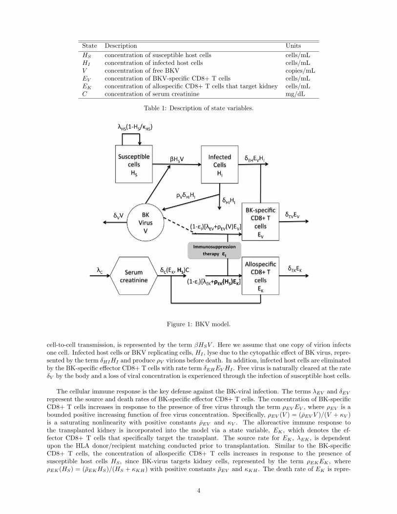
In this section we describe the dynamics of the viral load V , susceptible HS and infected HI host cells, BKV-specific EV and allospecific EK effector CD8+ T cells and serum creatinine C with a brief description of theunderlying biological model for which we base our mathematical model. Table 1 lists the state variables andFigure 1 diagrams the intracellular dynamics embodied in the model.

Active BKV infection targets both renal tubular epithelial cells and urothelial cells. For this model, how-ever, we focus on one BKV target, the renal tubular epithelial cells. Susceptible host cells, the uninfectedkidney tubular epithelial cells, HS , in the absence of infection, are assumed to proliferate through the termλHS

(1− HS

κHS

)HS , indicating that new epithelial cells are derived from proliferation of existing HS . Prolif-

eration is modeled by logistic dynamics with λHS being the maximum proliferation rate and κHS is the celldensity at which proliferation shuts off. A loss of susceptible cells, HS , due to viral infection which occurs by

3

State Description Units

HS concentration of susceptible host cells cells/mLHI concentration of infected host cells cells/mLV concentration of free BKV copies/mLEV concentration of BKV-specific CD8+ T cells cells/mLEK concentration of allospecific CD8+ T cells that target kidney cells/mLC concentration of serum creatinine mg/dL

Table 1: Description of state variables.

Figure 1: BKV model.

cell-to-cell transmission, is represented by the term βHSV . Here we assume that one copy of virion infectsone cell. Infected host cells or BKV replicating cells, HI , lyse due to the cytopathic effect of BK virus, repre-sented by the term δHIHI and produce ρV virions before death. In addition, infected host cells are eliminatedby the BK-specific effector CD8+ T cells with rate term δEHEV HI . Free virus is naturally cleared at the rateδV by the body and a loss of viral concentration is experienced through the infection of susceptible host cells.

The cellular immune response is the key defense against the BK-viral infection. The terms λEV and δEV

represent the source and death rates of BK-specific effector CD8+ T cells. The concentration of BK-specificCD8+ T cells increases in response to the presence of free virus through the term ρEV EV , where ρEV is abounded positive increasing function of free virus concentration. Specifically, ρEV (V ) = (ρEV V )/(V + κV )is a saturating nonlinearity with positive constants ρEV and κV . The alloreactive immune response tothe transplanted kidney is incorporated into the model via a state variable, EK , which denotes the ef-fector CD8+ T cells that specifically target the transplant. The source rate for EK , λEK , is dependentupon the HLA donor/recipient matching conducted prior to transplantation. Similar to the BK-specificCD8+ T cells, the concentration of allospecific CD8+ T cells increases in response to the presence ofsusceptible host cells HS , since BK-virus targets kidney cells, represented by the term ρEKEK , whereρEK(HS) = (ρEKHS)/(HS + κKH) with positive constants ρEV and κKH . The death rate of EK is repre-

4

sented by δEK .

Finally, we discuss the role of creatinine in the model. Creatinine is a waste product in the blood resultingfrom muscle activity and is removed by the healthy kidney. Therefore, serum creatinine concentration Cis used as a surrogate for glomerular filtration rate (GFR), a commonly used index of kidney function [?].The production rate of C is represented by λC and when the kidney is impaired, creatinine is not effectivelyfiltered and its concentration increases. To account for the negative effect of the alloreactive immune responseEK on the kidney and the positive effect of susceptible cells HS (Recall that the renal allograft is a site ofreplication. Hence, the concentration of susceptible cells reflects the health of the kidney.), the clearancerate δC is defined as follows

δC(EK ,HS) =δC0κEK

EK + κEK· HS

HS + κCH.

Table 2 lists the parameters used in the model. Based on the above discussion, the model is given as follows.

Parameter Description Parameter Description

λHS proliferation rate for HS κV saturation constantκHS saturation constant λEK source rate of EK

β infection rate of HS by V δEK death rate of EK

δHI death rate of HI by V λC production rate for CρV # virions produced by HI before death δC0 maximum clearance rate for CδEH elimination rate of HI by EV κEK saturation constantδV natural clearance rate of V κCH saturation constantλEV source rate of EV ρEK maximum proliferation rate for EK

δEV death rate of EV κKH saturation constantρEV maximum proliferation rate for EV εI efficacy of immunosuppressive drugs

Table 2: Model parameters and their corresponding descriptions.

HS = λHS

(1− HS

κHS

)HS − βHSV, (1)

HI = βHSV − δHIHI − δEHEV HI , (2)

V = ρV δHIHI − δV V − βHSV, (3)

EV = (1− ϵI)[λEV + ρEV (V )EV ]− δEV EV , (4)

EK = (1− ϵI)[λEK + ρEK(HS)EK ]− δEKEK , (5)

C = λC − δC(EK ,HS)C. (6)

with initial conditions,

(HS(0), HI(0), V (0), EV (0), EK(0), C(0)) = (HS0, HI0, V0, EV 0, EK0, C0). (7)

We note that (1)-(4) describe the immune response to the viral infection coupled with (5) and (6) describ-ing the immune response to the transplanted kidney. Here εI represents the efficacy of immunosuppressivedrugs and is assumed to be scaled to less than or equal to 1. This variable serves as the controller of thesystem to achieve balance between under-suppression and over-suppression of the patient’s immune system.

5

2.1 Data

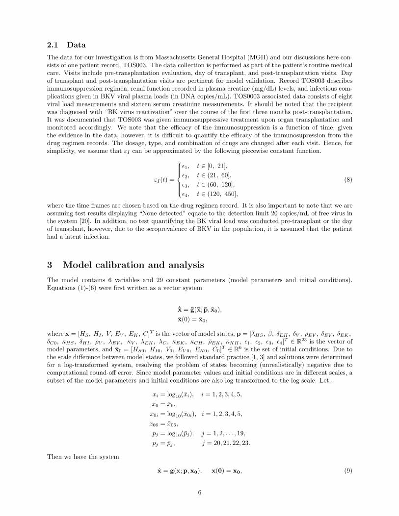
The data for our investigation is from Massachusetts General Hospital (MGH) and our discussions here con-sists of one patient record, TOS003. The data collection is performed as part of the patient’s routine medicalcare. Visits include pre-transplantation evaluation, day of transplant, and post-transplantation visits. Dayof transplant and post-transplantation visits are pertinent for model validation. Record TOS003 describesimmunosuppression regimen, renal function recorded in plasma creatine (mg/dL) levels, and infectious com-plications given in BKV viral plasma loads (in DNA copies/mL). TOS0003 associated data consists of eightviral load measurements and sixteen serum creatinine measurements. It should be noted that the recipientwas diagnosed with “BK virus reactivation” over the course of the first three months post-transplantation.It was documented that TOS003 was given immunosuppressive treatment upon organ transplantation andmonitored accordingly. We note that the efficacy of the immunosuppression is a function of time, giventhe evidence in the data, however, it is difficult to quantify the efficacy of the immunosupression from thedrug regimen records. The dosage, type, and combination of drugs are changed after each visit. Hence, forsimplicity, we assume that εI can be approximated by the following piecewise constant function.

εI(t) =

ϵ1, t ∈ [0, 21],

ϵ2, t ∈ (21, 60],

ϵ3, t ∈ (60, 120],

ϵ4, t ∈ (120, 450],

(8)

where the time frames are chosen based on the drug regimen record. It is also important to note that we areassuming test results displaying “None detected” equate to the detection limit 20 copies/mL of free virus inthe system [20]. In addition, no test quantifying the BK viral load was conducted pre-transplant or the dayof transplant, however, due to the seroprevalence of BKV in the population, it is assumed that the patienthad a latent infection.

3 Model calibration and analysis

The model contains 6 variables and 29 constant parameters (model parameters and initial conditions).Equations (1)-(6) were first written as a vector system

˙x = g(x; p, x0),

x(0) = x0,

where x = [HS , HI , V, EV , EK , C]T is the vector of model states, p = [λHS , β, δEH , δV , ρEV , δEV , δEK ,δC0, κHS , δHI , ρV , λEV , κV , λEK , λC , κEK , κCH , ρEK , κKH , ϵ1, ϵ2, ϵ3, ϵ4]

T ∈ R23 is the vector ofmodel parameters, and x0 = [HS0, HI0, V0, EV 0, EK0, C0]

T ∈ R6 is the set of initial conditions. Due tothe scale difference between model states, we followed standard practice [1, 3] and solutions were determinedfor a log-transformed system, resolving the problem of states becoming (unrealistically) negative due tocomputational round-off error. Since model parameter values and initial conditions are in different scales, asubset of the model parameters and initial conditions are also log-transformed to the log scale. Let,

xi = log10(xi), i = 1, 2, 3, 4, 5,

x6 = x6,

x0i = log10(x0i), i = 1, 2, 3, 4, 5,

x06 = x06,

pj = log10(pj), j = 1, 2, . . . , 19,

pj = pj , j = 20, 21, 22, 23.

Then we have the system

x = g(x;p,x0), x(0) = x0, (9)

6

where g = (g1, g2, . . . g6)T is given by

gi(x;p,x0) =10−xi

ln(10)gi(x; p, x0), i = 1, 2, . . . 5,

g6(x;p,x0) = g6(x; p, x0).

3.1 Forward simulations

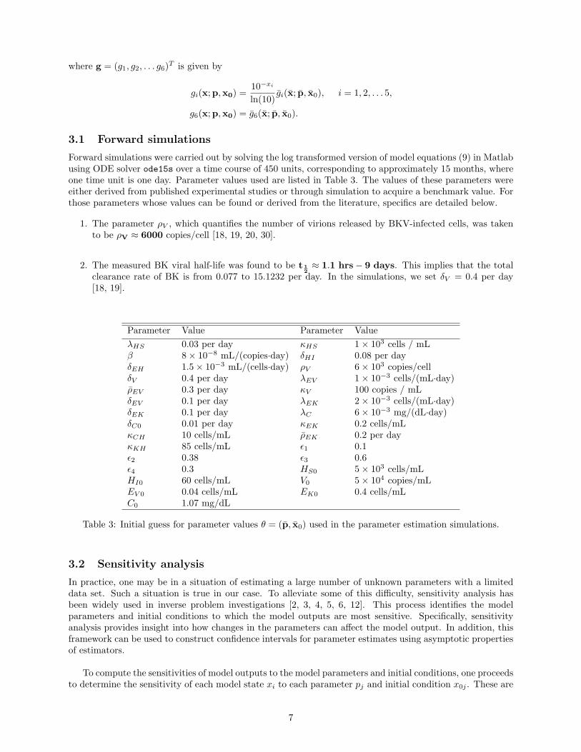
Forward simulations were carried out by solving the log transformed version of model equations (9) in Matlabusing ODE solver ode15s over a time course of 450 units, corresponding to approximately 15 months, whereone time unit is one day. Parameter values used are listed in Table 3. The values of these parameters wereeither derived from published experimental studies or through simulation to acquire a benchmark value. Forthose parameters whose values can be found or derived from the literature, specifics are detailed below.

1. The parameter ρV , which quantifies the number of virions released by BKV-infected cells, was takento be ρV ≈ 6000 copies/cell [18, 19, 20, 30].

2. The measured BK viral half-life was found to be t 12≈ 1.1 hrs− 9 days. This implies that the total

clearance rate of BK is from 0.077 to 15.1232 per day. In the simulations, we set δV = 0.4 per day[18, 19].

Parameter Value Parameter Value

λHS 0.03 per day κHS 1× 103 cells / mLβ 8× 10−8 mL/(copies·day) δHI 0.08 per dayδEH 1.5× 10−3 mL/(cells·day) ρV 6× 103 copies/cellδV 0.4 per day λEV 1× 10−3 cells/(mL·day)ρEV 0.3 per day κV 100 copies / mLδEV 0.1 per day λEK 2× 10−3 cells/(mL·day)δEK 0.1 per day λC 6× 10−3 mg/(dL·day)δC0 0.01 per day κEK 0.2 cells/mLκCH 10 cells/mL ρEK 0.2 per dayκKH 85 cells/mL ϵ1 0.1ϵ2 0.38 ϵ3 0.6ϵ4 0.3 HS0 5× 103 cells/mLHI0 60 cells/mL V0 5× 104 copies/mLEV 0 0.04 cells/mL EK0 0.4 cells/mLC0 1.07 mg/dL

Table 3: Initial guess for parameter values θ = (p, x0) used in the parameter estimation simulations.

3.2 Sensitivity analysis

In practice, one may be in a situation of estimating a large number of unknown parameters with a limiteddata set. Such a situation is true in our case. To alleviate some of this difficulty, sensitivity analysis hasbeen widely used in inverse problem investigations [2, 3, 4, 5, 6, 12]. This process identifies the modelparameters and initial conditions to which the model outputs are most sensitive. Specifically, sensitivityanalysis provides insight into how changes in the parameters can affect the model output. In addition, thisframework can be used to construct confidence intervals for parameter estimates using asymptotic propertiesof estimators.

To compute the sensitivities of model outputs to the model parameters and initial conditions, one proceedsto determine the sensitivity of each model state xi to each parameter pj and initial condition x0j . These are

7

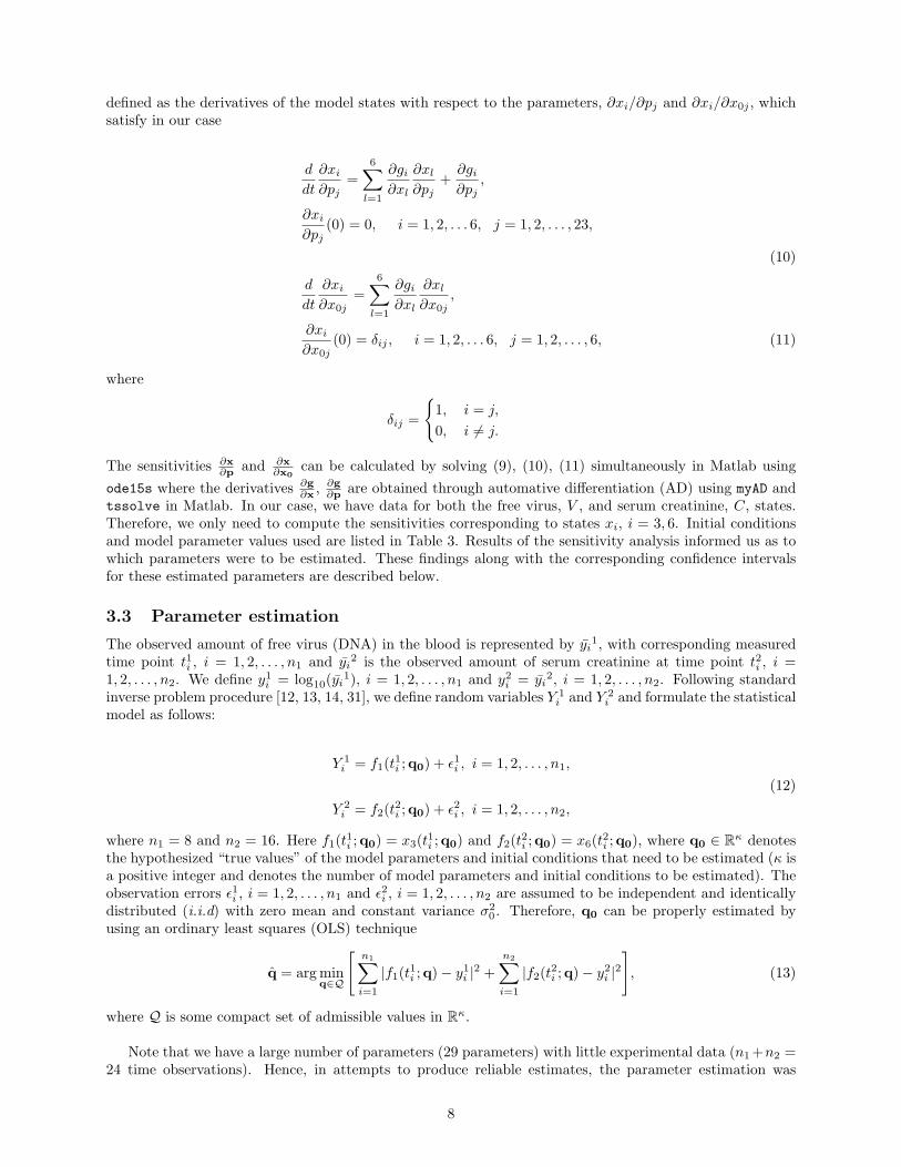
defined as the derivatives of the model states with respect to the parameters, ∂xi/∂pj and ∂xi/∂x0j , whichsatisfy in our case

d

dt

∂xi

∂pj=

6∑l=1

∂gi∂xl

∂xl

∂pj+

∂gi∂pj

,

∂xi

∂pj(0) = 0, i = 1, 2, . . . 6, j = 1, 2, . . . , 23,

(10)

d

dt

∂xi

∂x0j=

6∑l=1

∂gi∂xl

∂xl

∂x0j,

∂xi

∂x0j(0) = δij , i = 1, 2, . . . 6, j = 1, 2, . . . , 6, (11)

where

δij =

{1, i = j,

0, i = j.

The sensitivities ∂x∂p and ∂x

∂x0can be calculated by solving (9), (10), (11) simultaneously in Matlab using

ode15s where the derivatives ∂g∂x ,

∂g∂p are obtained through automative differentiation (AD) using myAD and

tssolve in Matlab. In our case, we have data for both the free virus, V , and serum creatinine, C, states.Therefore, we only need to compute the sensitivities corresponding to states xi, i = 3, 6. Initial conditionsand model parameter values used are listed in Table 3. Results of the sensitivity analysis informed us as towhich parameters were to be estimated. These findings along with the corresponding confidence intervalsfor these estimated parameters are described below.

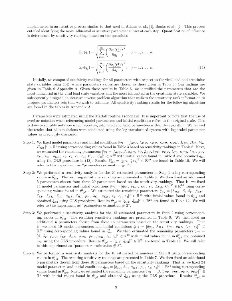
3.3 Parameter estimation

The observed amount of free virus (DNA) in the blood is represented by yi1, with corresponding measured

time point t1i , i = 1, 2, . . . , n1 and yi2 is the observed amount of serum creatinine at time point t2i , i =

1, 2, . . . , n2. We define y1i = log10(yi1), i = 1, 2, . . . , n1 and y2i = yi

2, i = 1, 2, . . . , n2. Following standardinverse problem procedure [12, 13, 14, 31], we define random variables Y 1

i and Y 2i and formulate the statistical

model as follows:

Y 1i = f1(t

1i ;q0) + ϵ1i , i = 1, 2, . . . , n1,

(12)

Y 2i = f2(t

2i ;q0) + ϵ2i , i = 1, 2, . . . , n2,

where n1 = 8 and n2 = 16. Here f1(t1i ;q0) = x3(t

1i ;q0) and f2(t

2i ;q0) = x6(t

2i ;q0), where q0 ∈ Rκ denotes

the hypothesized “true values” of the model parameters and initial conditions that need to be estimated (κ isa positive integer and denotes the number of model parameters and initial conditions to be estimated). Theobservation errors ϵ1i , i = 1, 2, . . . , n1 and ϵ2i , i = 1, 2, . . . , n2 are assumed to be independent and identicallydistributed (i.i.d) with zero mean and constant variance σ2

0 . Therefore, q0 can be properly estimated byusing an ordinary least squares (OLS) technique

q = argminq∈Q

[n1∑i=1

|f1(t1i ;q)− y1i |2 +n2∑i=1

|f2(t2i ;q)− y2i |2], (13)

where Q is some compact set of admissible values in Rκ.

Note that we have a large number of parameters (29 parameters) with little experimental data (n1+n2 =24 time observations). Hence, in attempts to produce reliable estimates, the parameter estimation was

8

implemented in an iterative process similar to that used in Adams et al., [1], Banks et al., [3]. This processentailed identifying the most influential or sensitive parameter subset at each step. Quantification of influenceis determined by sensitivity rankings based on the quantities

SV (qj) =

√√√√ n1∑k=1

(∂x3(t1k)

∂qj

)2

, j = 1, 2, . . . κ

SC(qj) =

√√√√ n2∑k=1

(∂x6(t2k)

∂qj

)2

, j = 1, 2, . . . κ. (14)

Initially, we computed sensitivity rankings for all parameters with respect to the viral load and creatininestate variables using (14), where parameters values are chosen as those given in Table 3. Our findings aregiven in Table 6 Appendix A. Given these results in Table 6, we identified the parameters that are themost influential in the viral load state variables and the most influential in the creatinine state variables. Wesubsequently designed an iterative inverse problem algorithm that utilizes the sensitivity rank information topropose parameters sets that we wish to estimate. All sensitivity ranking results for the following algorithmare found in the tables in Appendix A.

Parameters were estimated using the Matlab routine lsqnonlin. It is important to note that the use ofoverbar notation when referencing model parameters and initial conditions refers to the original scale. Thisis done to simplify notation when reporting estimated and fixed parameters within the algorithm. We remindthe reader that all simulations were conducted using the log-transformed system with log-scaled parametervalues as previously discussed.

Step 1: We fixed model parameters and initial conditions qU1 = [λEV , λEK , κEK , κCH , κKH , HS0, HI0, V0,EK0 ]

T ∈ R9 using corresponding values found in Table 3 based on sensitivity rankings in Table 6. Next,we estimated the remaining parameters qE1 = [λHS , β, δEH , δV , ρEV , δEV , δEK , δC0, κHS , δHI , ρV ,κV , λC , ρEK , ϵ1, ϵ2, ϵ3, ϵ4, EV 0, C0]

T ∈ R20 with initial values found in Table 3 and obtained qE1

using the OLS procedure in (13). Results θ1opt = [qU1, qE1]T ∈ R29 are found in Table 10. We will

refer to this experiment as “parameters estimation # 1”.

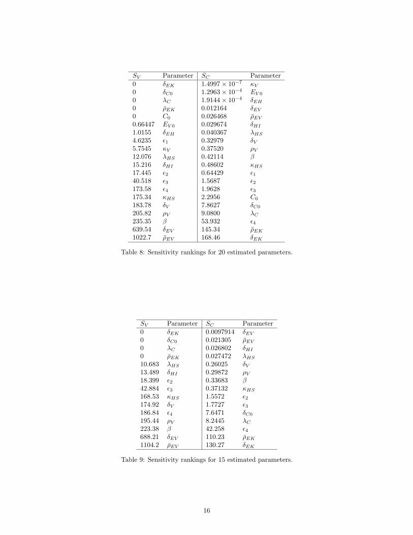
Step 2: We performed a sensitivity analysis for the 20 estimated parameters in Step 1 using correspondingvalues in θ1opt. The resulting sensitivity rankings are presented in Table 8. We then fixed an additional5 parameters chosen from these 20 parameters based on the sensitivity rankings. That is, we fixed14 model parameters and initial conditions qU2 = [qU1, δEH , κV , ϵ1, EV 0, C0]

T ∈ R14 using corre-sponding values found in θ1opt . We estimated the remaining parameters qE2 = [λHS , β, δV , ρEV ,

δEV , δEK , δC0, κHS , δHI , ρV , λC , ρEK , ϵ2, ϵ3, ϵ4]T ∈ R15 with initial values found in θ1opt and

obtained qE2 using OLS procedure. Results θ2opt = [qU2, qE2]T ∈ R29 are found in Table 12. We will

refer to this experiment as “parameters estimation # 2”.

Step 3: We performed a sensitivity analysis for the 15 estimated parameters in Step 2 using correspond-ing values in θ2opt. The resulting sensitivity rankings are presented in Table 9. We then fixed anadditional 5 parameters chosen from these 15 parameters based on the sensitivity rankings. Thatis, we fixed 19 model parameters and initial conditions qU3 = [qU2, λHS , δC0, δHI , λC , ϵ2]

T ∈R19 using corresponding values found in θ2opt. We then estimated the remaining parameters qE3 =

[β, δV , ρEV , δEV , δEK , κHS , ρV , ρEK , ϵ3, ϵ4]T ∈ R10 with initial values found in θ2opt and obtained

qE3 using the OLS procedure. Results θ3opt = [qU3, qE3]T ∈ R29 are found in Table 14. We will refer

to this experiment as “parameters estimation # 3”.

Step 4: We performed a sensitivity analysis for the 10 estimated parameters in Step 3 using correspondingvalues in θ3opt. The resulting sensitivity rankings are presented in Table 7. We then fixed an additional5 parameters chosen from these 10 parameters based on the sensitivity rankings. That is, we fixed 24model parameters and initial conditions qU4 = [qU3, δV , κHS , ρV , ϵ3, ϵ4]

T ∈ R24 using correspondingvalues found in θ3opt. Next, we estimated the remaining parameters qE4 = [β, ρEV , δEV , δEK , ρEK ]T ∈R5 with initial values found in θ3opt and obtained qE4 using the OLS procedure. Results θ4opt =

9

[qU4, qE4]T ∈ R29 are found in Table 4. We will refer to this experiment as “parameters estimation #

4”.

Next, we outline a method to quantify the uncertainty in our parameter estimations. Two methodsthat have been widely used in the literature to quantify uncertainty in parameter estimates are asymptotictheory and bootstrapping. Both have been investigated and compared in Banks et al. [7] for problems withdifferent form and level of noise. It was found that asymptotic theory is always faster computationally thanbootstrapping and there is no clear advantage in using bootstrapping versus asymptotic theory when theconstant variance using OLS is assumed. For these reasons, we will use asymptotic theory [4, 31] to quantifythe uncertainty in our parameter estimations.

We calculated standard errors and confidence intervals in order to quantify the uncertainty in parameterestimates. To compute these values, we must define some terms. Recall the statistical model defined in (12).Let

F(q) = (f1(t11;q), f1(t

12;q), . . . , f1(t

1n1;q), f2(t

21;q), f2(t

22;q), . . . , f2(t

2n2;q))T .

Then the sensitivity matrix χ(q) is an (n1 + n2) × κ matrix, where N = (n1 + n2) is the total number ofviral and creatinine data points and κ is the number of estimated parameters, with its (i, j)th element beingdefined as

χij(q) =∂Fi(q)

∂qj, i = 1, 2, . . . n1 + n2, j = 1, 2, . . . , κ, (15)

where Fi is the ith element of F , and qj is the jth element of q. Given the data {yi}Ni=1 = {y11 , y12 , . . . , y1n1, y21 , y

22 ,

. . . y2n2} and the resulting parameter estimate q, the variance σ2

0 can be approximated by

σ20 ≈ σ2 =

1

N − κ

N∑j=1

[yj −Fj(q)]2. (16)

With these values, we can calculateΣ(q) = σ2[χ(q)Tχ(q)]−1. (17)

This matrix is known as the covariance matrix and is used to compute the standard errors for each elementof q given by

SEk(q) =

√Σkk(q), k = 1, 2, . . . κ. (18)

Hence, the 100(1− α)% confidence intervals are given by

[qk − t1−α/2SEk(q), qk + t1−α/2SEk(q)]. (19)

We determine t1−α/2 by Prob{T ≥ t1−α/2} = α/2, where T has a student’s t distribution tN−κ with N − κdegrees of freedom.

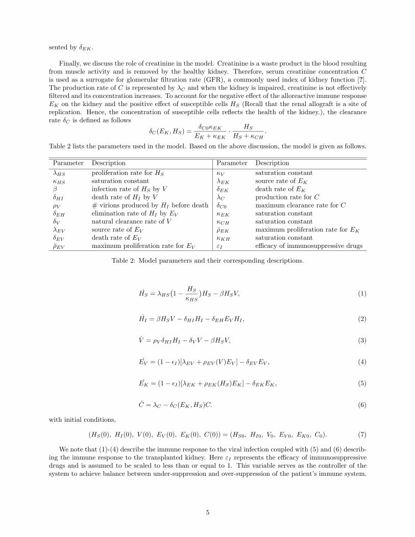
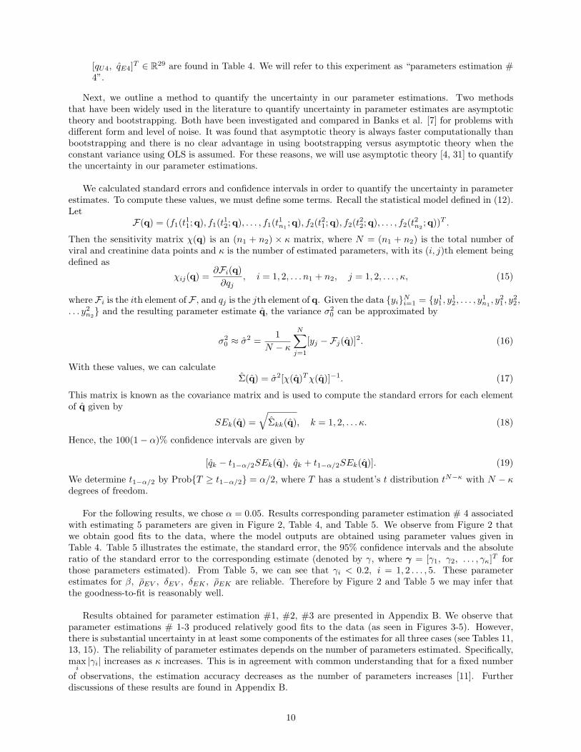
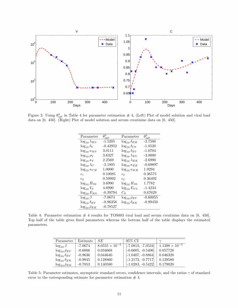
For the following results, we chose α = 0.05. Results corresponding parameter estimation # 4 associatedwith estimating 5 parameters are given in Figure 2, Table 4, and Table 5. We observe from Figure 2 thatwe obtain good fits to the data, where the model outputs are obtained using parameter values given inTable 4. Table 5 illustrates the estimate, the standard error, the 95% confidence intervals and the absoluteratio of the standard error to the corresponding estimate (denoted by γ, where γ = [γ1, γ2, . . . , γκ]

T forthose parameters estimated). From Table 5, we can see that γi < 0.2, i = 1, 2 . . . , 5. These parameterestimates for β, ρEV , δEV , δEK , ρEK are reliable. Therefore by Figure 2 and Table 5 we may infer thatthe goodness-to-fit is reasonably well.

Results obtained for parameter estimation #1, #2, #3 are presented in Appendix B. We observe thatparameter estimations # 1-3 produced relatively good fits to the data (as seen in Figures 3-5). However,there is substantial uncertainty in at least some components of the estimates for all three cases (see Tables 11,13, 15). The reliability of parameter estimates depends on the number of parameters estimated. Specifically,max

i|γi| increases as κ increases. This is in agreement with common understanding that for a fixed number

of observations, the estimation accuracy decreases as the number of parameters increases [11]. Furtherdiscussions of these results are found in Appendix B.

10

0 100 200 300 40010

0

102

104

106

Days

V

ModelData

0 100 200 300 400

0.65

0.7

0.75

0.8

0.85

0.9

0.95

1

1.05

1.1

Days

C

ModelData

Figure 2: Using θ4opt in Table 4 for parameter estimation # 4, (Left) Plot of model solution and viral loaddata on [0, 450]. (Right) Plot of model solution and serum creatinine data on [0, 450].

Parameter θ4opt Parameter θ4optlog10 λHS -1.5205 log10 δEH -2.7500log10 δV -0.42952 log10 δC0 -1.8520log10 κHS 3.0111 log10 δHI -1.0704log10 ρV 3.6327 log10 λEV -3.0000log10 κV 2.2569 log10 λEK -2.6990log10 λC -2.1805 log10 κEK -0.69897log10 κCH 1.0000 log10 κKH 1.9294ϵ1 0.10085 ϵ2 0.36575ϵ3 0.59992 ϵ4 0.36492log10 HS0 3.6990 log10 HS0 1.7782log10 V0 4.6990 log10 EV 0 -1.4234log10 EK0 -0.39794 C0 0.67629log10 β -7.0674 log10 ρEV -0.60055log10 δEV -0.96356 log10 δEK -0.99450log10 ρEK -0.78527

Table 4: Parameter estimation # 4 results for TOS003 viral load and serum creatinine data on [0, 450].Top half of the table gives fixed parameters whereas the bottom half of the table displays the estimatedparameters.

Parameter Estimate SE 95% CI γlog10 β -7.0674 8.0555× 10−3 [-7.0813, -7.0534] 1.1398× 10−3

log10 ρEV -0.6006 0.034668 [-0.6605, -0.5406] 0.057728log10 δEV -0.9636 0.044640 [-1.0407, -0.8864] 0.046328log10 δEK -0.9945 0.128860 [-1.2173, -0.7717] 0.129580log10 ρEK -0.7853 0.140580 [-1.0283, -0.5422] 0.179020

Table 5: Parameter estimates, asymptotic standard errors, confidence intervals, and the ratios γ of standarderror to the corresponding estimate for parameter estimation # 4.

11

4 Concluding remarks and future research effort

Our efforts here to develop a mathematical model with statistically based model validation can be properlyviewed as an algorithmic approach to determining the information content in a specific experimental data set.That is, we illustrate one approach to determining how many and which model parameters can be estimatedwith confidence from a given data set. In this context we have developed an initial mechanistic mathematicalmodel to describe the immune response to both BKV infection and a donor kidney, and have estimated modelparameters and initial conditions using the clinical data. Due to the large number of unknown parametersand limited number of observations, one is unable to reliably estimate all the parameters. To alleviate thisdifficulty, we employed sensitivity analysis combined with asymptotic theory of estimators to determine thenumber of parameters that can be reliably estimated. Numerical results show that we were able to reliablyestimate five parameters with the given eight viral load data points and sixteen creatinine data points. Thisclearly demonstrates that one requires more informative longitudinal data, particularly observations on othermodel variables, in order to fully validate the model. In this context an immediate future effort would beto use optimal design methods (e.g., [9, 10]) to determine when an experimenter should take measurementsand what model variables to measure. The obtained results should then be used to guide the future datacollection efforts.

Acknowledgments

This research was supported in part by grant number NIAID R01AI071915-10 from the National Instituteof Allergy and Infectious Diseases, in part by the Air Force Office of Scientific Research under grant numberAFOSR FA9550-12-1-0188, and in part by the National Science Foundation under Research Training Grant(RTG) DMS-1246991.

References

[1] B.M. Adams, H.T. Banks, M. Davidian, and E.S. Rosenberg, Model fitting and prediction with HIVtreatment interruption data, Bull. Math. Biol., 69 (2005), 563–584.

[2] H.T. Banks, A. Cintron-Arias, and F. Kappel, Parameter selection methods in inverse problem for-mulation, CRSC Tech. Report CRSC-TR10-03 (2010), NCSU, Raleigh; in Mathematical Modeling andValidation in Physiology: Application to the Cardiovascular and Respiratory Systems,(J. J. Batzel, M.Bachar, and F. Kappel, eds.), pp. 43 - 73, Lecture Notes in Mathematics Vol. 2064, Springer-Verlag,Berlin 2013.

[3] H.T. Banks, M. Davidian, S. Hu, G.M. Kepler, and E.S. Rosenberg, Modelling HIV immune responseand validation with clinical data, J. Biol. Dyn., 2 (2008), 357–385.

[4] H.T. Banks, M. Davidian, J.R. Samuels Jr., and K.L. Sutton, An inverse problem statistical methodologysummary, CRSC Tech. Report CRSC-TR08-01, (2008), NCSU, Raleigh; In: G. Chowell, M. Hyman,N. Hengartner, L.M.A. Bettencourt, C. Castillo-Chavez (Eds.), Statistical Estimation Approaches inEpidemiology, Springer, Berlin, Heidelberg, New York (2009), 249–302.

[5] H.T. Banks, S. Dediu, S.L. Ernstberger, and F. Kappel, Generalized sensitivities and optimal experi-mental design, Center for Research in Scientific Computation Report, CRSC-TR08-12 (revised) (2008),NCSU, Raleigh; J. Inverse and Ill-Posed Problems, 8 (2010), 25–83.

[6] H.T. Banks, K.J. Holm, and F. Kappel, Comparison of optimal design methods in inverse problems,Tech. Report CRSC-TR10-11 (2010), NCSU, Raleigh; Inverse Problems 27 (2011), 075002.

[7] H.T. Banks, K. Holm, and D. Robbins, Standard error computations for uncertainty quantification ininverse problems: asymptotic theory vs. bootstrapping, CRSC Technical Report CRSC-TR09-13, NCSU,May 2010; Mathematical and Computer Modeling, 52 (2010), 1610-1625.

[8] H.T. Banks, S. Hu, T. Jang, and H.D. Kwon, Modeling and optimal control of immune response of renaltransplant recipients, J. Biol. Dyn., 6 (2012), 539–567.

12

[9] H.T. Banks and K.L. Rehm, Experimental design for vector output systems, CRSC Tech. Re-port CRSC-TR12-11, April, 2012; Inverse Problems in Sci. and Engr., (2013), 1–34. DOI:10.1080/17415977.2013.797973

[10] H.T. Banks and K.L. Rehm, Experimental design for distributed parameter vector systems, CRSCTech. Report CRSC-TR12-17, August, 2012; Applied Mathematics Letters, 26 (2013), 10–14;http://dx.doi.org/10.1016/j.aml.2012.08.003.

[11] H.T. Banks, S. Hu, and W.C. Thompson, Modeling and Inverse Problems in the Presence of Uncertainty,Taylor/Francis-Chapman/Hall-CRC Press, Boca Raton, FL, 2014.

[12] H.T. Banks and H.T. Tran, Mathematical and Experimental Modeling of Physical and Biological Pro-cesses, Taylor/Francis-Chapman/Hall-CRC Press, Boca Raton, FL, 2009.

[13] R.J. Carrol and D. Ruppert, Transformation and Weighting in Regression, Chapman & Hall, New York,1988).

[14] M. Davidian and D. Giltinan, Nonlinear Models for Repeated Measurement Data, Chapman & Hall,London, 1998.

[15] United States Department of Health and Human Services, (n.d.). OPTN,SRTR Annual Report, 2011,8-10. Retrieved May 12, 2014 from the World Wide Web: http://optn.transplant.hrsa.gov.

[16] S. Eash, W. Querbes, and W.J. Atwood, Infection of vero cells by BK virus is dependent on caveolae,Journal of Virology, 78 (2004), 11583–11590.

[17] A. Egli, S. Binggeli, S. Bodaghi, et. al., Cytomegalovirus and polyomavirus BK post-transplant, Nephrol.Dial. Transplant, 22 (2007), viii72–viii82.

[18] G.A. Funk, R. Gosert, P. Comoli, F. Ginevri, and H. H. Hirsch, Polyomavirus BK replication dynamicsin vivo and in silico to predict cytopathology and viral clearance in kidney transplants, American Journalof Transplantation, 8 (2008), 2368–2377.

[19] G.A. Funk, and H.H. Hirsch, From plasma BK viral load to allograft damage: Rule of thumb forestimating the intrarenal cytopathic wear, Clinical Infectious Diseases, 49 (2009), 989–990.

[20] G.A. Funk, J. Steiger, and H.H. Hirsch, Rapid dynamics of polyomavirus type BK in renal transplantrecipients, Journal Infectious Diseases, 190 (2006), 80–87.

[21] S.D. Gardner, A.M. Field, D.V. Coleman, and B. Hulme, New human papovavirus (B.K.) isolated fromurine after renal transplantation, Lancet, 297 (1971), 1253-1257.

[22] M.H. Hammer, G. Brestrich, H. Andreee, et al., HLA Type-independent method to monitor polymaBK virus-specific CD4+ and CD8+ T-cell immunity, American Journal of Transplantation, 6 (2006),625–631.

[23] J. Heritage, P.M. Chesters, and D.J. McCance, The persistence of papovavirus BK DNA sequences innormal human renal tissue, J. Med. Virol., 8 (1981), 142–150.

[24] H. H. Hirsch, BK virus: opportunity makes a pathogen, Clinical Infectious Disease, 41 (2005), 354–360.

[25] H.H. Hirsch and J. Steiger, Polyomavirus BK. Lancet Infectious Diseases 3 (2003), 611–623.

[26] G.M. Kepler, H.T. Banks, M. Davidian, and E.S. Rosenberg, A model for HCMV Infection in Immuno-suppressed Patients, Mathematical and Computer Modelling, 49 (2005), 1653–1663.

[27] W.A. Knowles, P. Pipkin, N. Andrews, A. Vyse, P. Minor, D.W. Brown, and E. Miller, Population-basedstudy of antibody to the human polyomaviruses BKV and JCV and the simian polyomavirus SV40, J.Med. Virol., 71 (2003), 115–123.

[28] V. Nickeleit, H.H. Hirsch, I.F. Binet, et al., Polyomavirus infection of renal allograft recipients: Fromlatent infection to manifest disease, J. Am. Soc. Nephrol., 10 (1999), 1080–1089.

13

[29] E. Ramos, C.B. Drachenberg, M. Portocarrero, et al., BK virus nephrology diagnosis and treatment:experience at the University of Maryland Renal Transplant Program, Clin Transpl. (2002), 143–153.

[30] P.S. Randhawa, A. Vats, D. Zygmunt, P. Swalsky, V. Scantlebury, R. Shapiro, and S. Finkelstein,Quantification of viral DNA in renal allograft tissue from patients with BK virus nephropathy, Transplant,74 (2002), 485–488.

[31] G.A. Sever and C.J. Wild, Nonlinear Regression Wiley, Hoboken NJ, 2003.

14

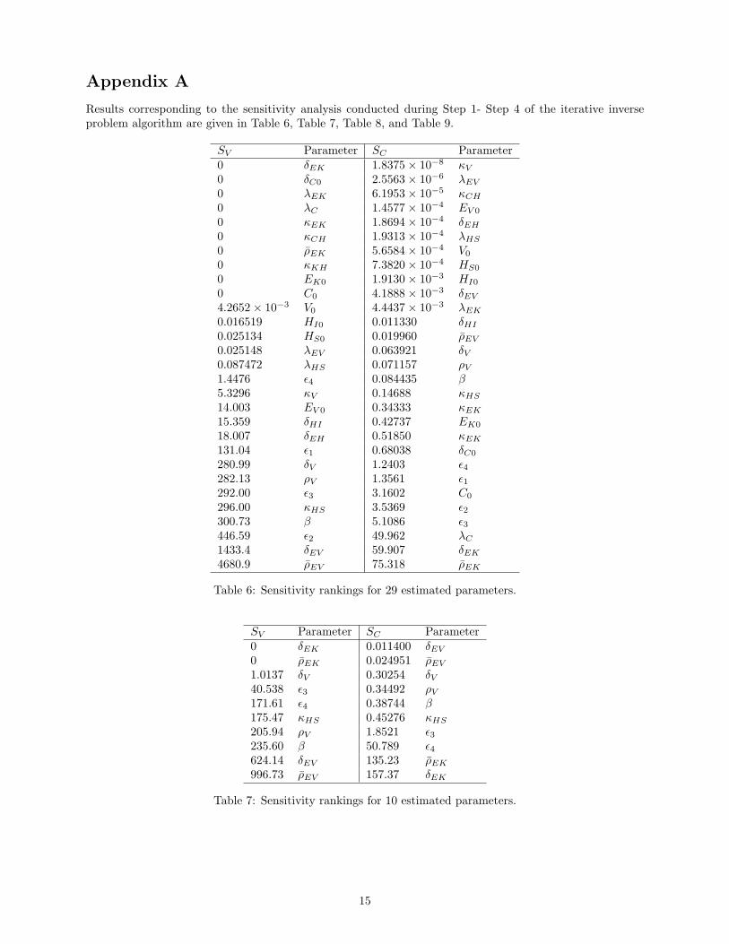
Appendix A

Results corresponding to the sensitivity analysis conducted during Step 1- Step 4 of the iterative inverseproblem algorithm are given in Table 6, Table 7, Table 8, and Table 9.

SV Parameter SC Parameter0 δEK 1.8375× 10−8 κV

0 δC0 2.5563× 10−6 λEV

0 λEK 6.1953× 10−5 κCH

0 λC 1.4577× 10−4 EV 0

0 κEK 1.8694× 10−4 δEH

0 κCH 1.9313× 10−4 λHS

0 ρEK 5.6584× 10−4 V0

0 κKH 7.3820× 10−4 HS0

0 EK0 1.9130× 10−3 HI0

0 C0 4.1888× 10−3 δEV

4.2652× 10−3 V0 4.4437× 10−3 λEK

0.016519 HI0 0.011330 δHI

0.025134 HS0 0.019960 ρEV

0.025148 λEV 0.063921 δV0.087472 λHS 0.071157 ρV1.4476 ϵ4 0.084435 β5.3296 κV 0.14688 κHS

14.003 EV 0 0.34333 κEK

15.359 δHI 0.42737 EK0

18.007 δEH 0.51850 κEK

131.04 ϵ1 0.68038 δC0

280.99 δV 1.2403 ϵ4282.13 ρV 1.3561 ϵ1292.00 ϵ3 3.1602 C0

296.00 κHS 3.5369 ϵ2300.73 β 5.1086 ϵ3446.59 ϵ2 49.962 λC

1433.4 δEV 59.907 δEK

4680.9 ρEV 75.318 ρEK

Table 6: Sensitivity rankings for 29 estimated parameters.

SV Parameter SC Parameter0 δEK 0.011400 δEV

0 ρEK 0.024951 ρEV

1.0137 δV 0.30254 δV40.538 ϵ3 0.34492 ρV171.61 ϵ4 0.38744 β175.47 κHS 0.45276 κHS

205.94 ρV 1.8521 ϵ3235.60 β 50.789 ϵ4624.14 δEV 135.23 ρEK

996.73 ρEV 157.37 δEK

Table 7: Sensitivity rankings for 10 estimated parameters.

15

SV Parameter SC Parameter0 δEK 1.4997× 10−7 κV

0 δC0 1.2963× 10−4 EV 0

0 λC 1.9144× 10−4 δEH

0 ρEK 0.012164 δEV

0 C0 0.026468 ρEV

0.66447 EV 0 0.029674 δHI

1.0155 δEH 0.040367 λHS

4.6235 ϵ1 0.32979 δV5.7545 κV 0.37520 ρV12.076 λHS 0.42114 β15.216 δHI 0.48602 κHS

17.445 ϵ2 0.64429 ϵ140.518 ϵ3 1.5687 ϵ2173.58 ϵ4 1.9628 ϵ3175.34 κHS 2.2956 C0

183.78 δV 7.8627 δC0

205.82 ρV 9.0800 λC

235.35 β 53.932 ϵ4639.54 δEV 145.34 ρEK

1022.7 ρEV 168.46 δEK

Table 8: Sensitivity rankings for 20 estimated parameters.

SV Parameter SC Parameter0 δEK 0.0097914 δEV

0 δC0 0.021305 ρEV

0 λC 0.026802 δHI

0 ρEK 0.027472 λHS

10.683 λHS 0.26025 δV13.489 δHI 0.29872 ρV18.399 ϵ2 0.33683 β42.884 ϵ3 0.37132 κHS

168.53 κHS 1.5572 ϵ2174.92 δV 1.7727 ϵ3186.84 ϵ4 7.6471 δC0

195.44 ρV 8.2445 λC

223.38 β 42.258 ϵ4688.21 δEV 110.23 ρEK

1104.2 ρEV 130.27 δEK

Table 9: Sensitivity rankings for 15 estimated parameters.

16

Appendix B

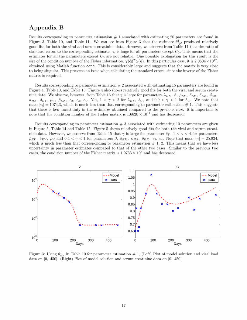
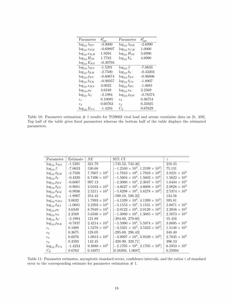
Results corresponding to parameter estimation # 1 associated with estimating 20 parameters are found inFigure 3, Table 10, and Table 11. We can see from Figure 3 that the estimate θ1opt produced relativelygood fits for both the viral and serum creatinine data. However, we observe from Table 11 that the ratio ofstandard errors to the corresponding estimate, γ, is huge for all parameters except C0. This means that theestimates for all the parameters except C0 are not reliable. One possible explanation for this result is thesize of the condition number of the Fisher information, χ(q)Tχ(q). In this particular case, it is 2.0604×1017,obtained using Matlab function cond. This is considerably large and suggests that the matrix is very closeto being singular. This presents an issue when calculating the standard errors, since the inverse of the Fishermatrix is required.

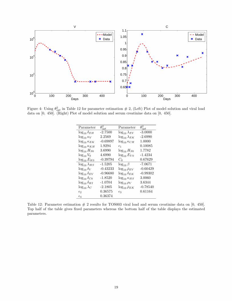
Results corresponding to parameter estimation # 2 associated with estimating 15 parameters are found inFigure 4, Table 10, and Table 13. Figure 4 also shows relatively good fits for both the viral and serum creati-nine data. We observe, however, from Table 13 that γ is large for parameters λHS , β, ρEV , δEV , δEK , δC0,κHS , δHI , ρV , ρEK , ϵ2, ϵ3, ϵ4. Yet, 1 < γ < 2 for λHS , δC0 and 0.9 < γ < 1 for λC . We note thatmaxi |γi| = 1074.3, which is much less than that corresponding to parameter estimation # 1. This suggeststhat there is less uncertainty in the estimates obtained compared to the previous case. It is important tonote that the condition number of the Fisher matrix is 1.6620× 1011 and has decreased.

Results corresponding to parameter estimation # 3 associated with estimating 10 parameters are givenin Figure 5, Table 14 and Table 15. Figure 5 shows relatively good fits for both the viral and serum creati-nine data. However, we observe from Table 15 that γ is large for parameter δV , 1 < γ < 4 for parametersρEV , δEV , ρV and 0.4 < γ < 1 for parameters β, δEK , κHS , ρEK , ϵ3, ϵ4. Note that maxi |γi| = 25.924,which is much less than that corresponding to parameter estimation # 1, 2. This means that we have lessuncertainty in parameter estimates compared to that of the other two cases. Similar to the previous twocases, the condition number of the Fisher matrix is 1.9733× 108 and has decreased.

0 100 200 300 40010

0

102

104

106

Days

V

ModelData

0 100 200 300 400

0.65

0.7

0.75

0.8

0.85

0.9

0.95

1

1.05

1.1

Days

C

ModelData

Figure 3: Using θ1opt in Table 10 for parameter estimation # 1, (Left) Plot of model solution and viral loaddata on [0, 450]. (Right) Plot of model solution and serum creatinine data on [0, 450].

17

Parameter θ1opt Parameter θ1optlog10 λEV -3.0000 log10 λEK -2.6990log10 κEK -0.69897 log10 κCH 1.0000log10 κKH 1.9294 log10 HS0 3.6990log10 HS0 1.7782 log10 V0 4.6990log10 EK0 -0.39794log10 λHS -1.5291 log10 β -7.0633log10 δEH -2.7500 log10 δV -0.43203log10 ρEV -0.60674 log10 δEV -0.96806log10 δEK -0.99357 log10 δC0 -1.8907log10 κHS 3.0032 log10 δHI -1.0681log10 ρV 3.6349 log10 κV 2.2569log10 λC -2.1994 log10 ρEK -0.78374ϵ1 0.10085 ϵ2 0.36754ϵ3 0.60763 ϵ4 0.35925log10 EV 0 -1.4234 C0 0.67629

Table 10: Parameter estimation # 1 results for TOS003 viral load and serum creatinine data on [0, 450].Top half of the table gives fixed parameters whereas the bottom half of the table displays the estimatedparameters.

Parameter Estimate SE 95% CI γlog10 λHS -1.5291 321.79 [-745.52, 742.46] 210.45log10 β -7.0633 530.68 [−1.2340× 103, 1.2199× 103] 75.131log10 δEH -2.7500 7.7607× 105 [−1.7943× 106, 1.7943× 106] 2.8221× 105

log10 δV -0.4320 6.7490× 103 [−1.5604× 104, 1.5603× 104] 1.5622× 104

log10 ρEV -0.6067 997.13 [−2.3060× 103, 2.3047× 103] 1.6434× 103

log10 δEV -0.9681 2.0163× 103 [−4.6627× 103, 4.6608× 103] 2.0828× 103

log10 δEK -0.9936 2.5211× 103 [−5.8298× 103, 5.8278× 103] 2.5374× 103

log10 δC0 -1.8907 254.42 [-590.10, 586.32] 134.56log10 κHS 3.0032 1.7893× 103 [−4.1339× 103, 4.1399× 103] 595.81log10 δHI -1.0681 2.2293× 103 [−5.1553× 103, 5.1531× 103] 2.0871× 103

log10 ρV 3.6349 8.7049× 103 [−2.0122× 104, 2.0129× 104] 2.3948× 103

log10 κV 2.2569 5.6586× 103 [−1.3080× 104, 1.3085× 104] 2.5073× 103

log10 λC -2.1994 121.88 [-284.00, 279.60] 55.416log10 ρEK -0.7837 2.4214× 103 [−5.5990× 103, 5.5974× 103] 3.0895× 103

ϵ1 0.1009 1.5278× 103 [−3.5321× 103, 3.5323× 103] 1.5148× 104

ϵ2 0.3675 128.05 [-295.69, 296.43] 348.40ϵ3 0.6076 1.6913× 103 [−3.9097× 103, 3.9109× 103] 2.7835× 103

ϵ4 0.3593 142.45 [-328.99, 329.71] 396.53log10 EV 0 -1.4234 9.3880× 105 [−2.1705× 106, 2.1705× 106] 6.5953× 105

C0 0.6763 0.16971 [0.28393, 1.0687] 0.25094

Table 11: Parameter estimates, asymptotic standard errors, confidence intervals, and the ratios γ of standarderror to the corresponding estimate for parameter estimation # 1.

18

0 100 200 300 40010

0

102

104

106

Days

V

ModelData

0 100 200 300 400

0.65

0.7

0.75

0.8

0.85

0.9

0.95

1

1.05

1.1

Days

C

ModelData

Figure 4: Using θ2opt in Table 12 for parameter estimation # 2, (Left) Plot of model solution and viral loaddata on [0, 450]. (Right) Plot of model solution and serum creatinine data on [0, 450].

Parameter θ2opt Parameter θ2optlog10 δEH -2.7500 log10 λEV -3.0000log10 κV 2.2569 log10 λEK -2.6990log10 κEK -0.69897 log10 κCH 1.0000log10 κKH 1.9294 ϵ1 0.10085log10 HS0 3.6990 log10 HS0 1.7782log10 V0 4.6990 log10 EV 0 -1.4234log10 EK0 -0.39794 C0 0.67629log10 λHS -1.5205 log10 β -7.0671log10 δV -0.43233 log10 ρEV -0.60429log10 δEV -0.96680 log10 δEK -0.99302log10 δC0 -1.8520 log10 κHS 3.0060log10 δHI -1.0704 log10 ρV 3.6344log10 λC -2.1805 log10 ρEK -0.78540ϵ2 0.36575 ϵ3 0.61164ϵ4 0.36374

Table 12: Parameter estimation # 2 results for TOS003 viral load and serum creatinine data on [0, 450].Top half of the table gives fixed parameters whereas the bottom half of the table displays the estimatedparameters.

19

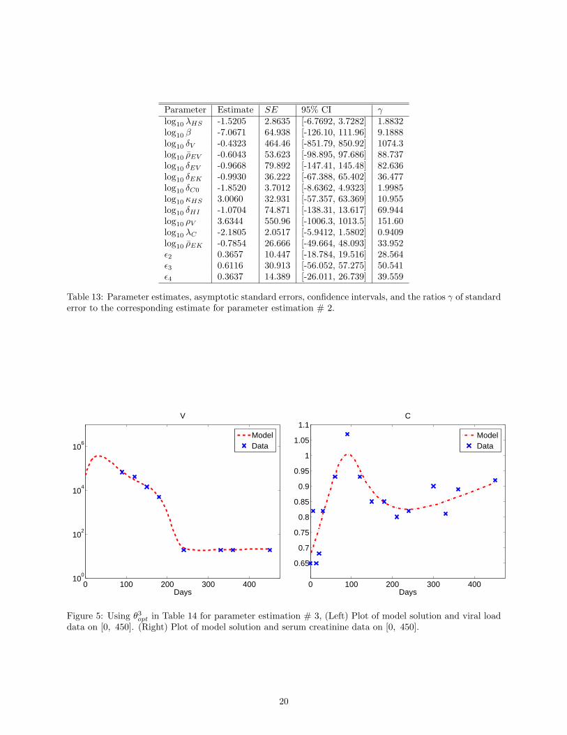
Parameter Estimate SE 95% CI γlog10 λHS -1.5205 2.8635 [-6.7692, 3.7282] 1.8832log10 β -7.0671 64.938 [-126.10, 111.96] 9.1888log10 δV -0.4323 464.46 [-851.79, 850.92] 1074.3log10 ρEV -0.6043 53.623 [-98.895, 97.686] 88.737log10 δEV -0.9668 79.892 [-147.41, 145.48] 82.636log10 δEK -0.9930 36.222 [-67.388, 65.402] 36.477log10 δC0 -1.8520 3.7012 [-8.6362, 4.9323] 1.9985log10 κHS 3.0060 32.931 [-57.357, 63.369] 10.955log10 δHI -1.0704 74.871 [-138.31, 13.617] 69.944log10 ρV 3.6344 550.96 [-1006.3, 1013.5] 151.60log10 λC -2.1805 2.0517 [-5.9412, 1.5802] 0.9409log10 ρEK -0.7854 26.666 [-49.664, 48.093] 33.952ϵ2 0.3657 10.447 [-18.784, 19.516] 28.564ϵ3 0.6116 30.913 [-56.052, 57.275] 50.541ϵ4 0.3637 14.389 [-26.011, 26.739] 39.559

Table 13: Parameter estimates, asymptotic standard errors, confidence intervals, and the ratios γ of standarderror to the corresponding estimate for parameter estimation # 2.

0 100 200 300 40010

0

102

104

106

Days

V

ModelData

0 100 200 300 400

0.65

0.7

0.75

0.8

0.85

0.9

0.95

1

1.05

1.1

Days

C

ModelData

Figure 5: Using θ3opt in Table 14 for parameter estimation # 3, (Left) Plot of model solution and viral loaddata on [0, 450]. (Right) Plot of model solution and serum creatinine data on [0, 450].

20

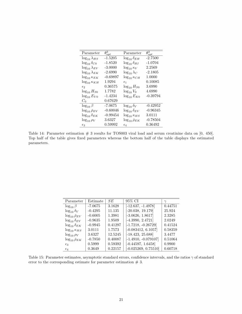
Parameter θ3opt Parameter θ3optlog10 λHS -1.5205 log10 δEH -2.7500log10 δC0 -1.8520 log10 δHI -1.0704log10 λEV -3.0000 log10 κV 2.2569log10 λEK -2.6990 log10 λC -2.1805log10 κEK -0.69897 log10 κCH 1.0000log10 κKH 1.9294 ϵ1 0.10085ϵ2 0.36575 log10 HS0 3.6990log10 HS0 1.7782 log10 V0 4.6990log10 EV 0 -1.4234 log10 EK0 -0.39794C0 0.67629log10 β -7.0675 log10 δV -0.42952log10 ρEV -0.60046 log10 δEV -0.96345log10 δEK -0.99454 log10 κHS 3.0111log10 ρV 3.6327 log10 ρEK -0.78504ϵ3 0.59992 ϵ4 0.36492

Table 14: Parameter estimation # 3 results for TOS003 viral load and serum creatinine data on [0, 450].Top half of the table gives fixed parameters whereas the bottom half of the table displays the estimatedparameters.

Parameter Estimate SE 95% CI γlog10 β -7.0675 3.1628 [-12.637, -1.4978] 0.44751log10 δV -0.4295 11.135 [-20.038, 19.179] 25.924log10 ρEV -0.6005 1.3981 [-3.0626, 1.8617] 2.3285log10 δEV -0.9635 1.9509 [-4.3990, 2.4721] 2.0249log10 δEK -0.9945 0.41297 [-1.7218, -0.26729] 0.41524log10 κHS 3.0111 1.7573 [-0.083412, 6.1057] 0.58359log10 ρV 3.6327 12.5245 [-18.423, 25.688] 3.4477log10 ρEK -0.7850 0.40087 [-1.4910, -0.079107] 0.51064ϵ3 0.5999 0.59392 [-0.44597, 1.6458] 0.9900ϵ4 0.3649 0.22157 [-0.025269, 0.75510] 0.60718

Table 15: Parameter estimates, asymptotic standard errors, confidence intervals, and the ratios γ of standarderror to the corresponding estimate for parameter estimation # 3.

21