
Modeling Growth Curve of Fractal Dimension of Urban Form ...
37
1 Modeling Growth Curve of Fractal Dimension of Urban Form of Beijing Yanguang Chen; Linshan Huang (Department of Geography, College of Urban and Environmental Sciences, Peking University, Beijing 100871, P.R.China. E-mail: [email protected]) Abstract: The growth curves of fractal dimension of urban form take on squashing effect and can be described by sigmoid functions. The fractal dimension growth of urban form in western countries can be modeled by Boltzmann’s equation and logistic function. However, these models cannot be well applied to the fractal dimension growth curve of Beijing city, the national capital of China. In this paper, the experimental method is employed to find parametric models for the growth curves of fractal dimension of Chinese urban form. By statistical analysis, numerical analysis, and comparative analysis, we find that the quadratic Boltzmann equation and quadratic logistic function can be used to characterize how the fractal dimension of the urban land-use pattern of Beijing increases in the course of time. The models are also suitable for many cities in the north of China. In order to convert the empirical models into theoretical models, we attempt to construct a model of spatial replacement dynamics of urban evolution, from which the logistic model of urban fractal dimension growth can be derived. The models can be utilized to predict the rate and upper limitation of Chinese urban growth. In particular, the models can be employed to reveal the similarities and differences between the fractal growth of Chinese cities and that of the cities in western countries. Key words: multifractals; quadratic Boltzmann’s equation; quadratic logistic function; spatial replacement dynamics; urban form; urban growth 1. Introduction Fractal geometry is one of effective means of describing complex systems and exploring
Transcript of Modeling Growth Curve of Fractal Dimension of Urban Form ...

1
Modeling Growth Curve of Fractal Dimension of
Urban Form of Beijing
Yanguang Chen; Linshan Huang
(Department of Geography, College of Urban and Environmental Sciences, Peking University, Beijing
100871, P.R.China. E-mail: [email protected])
Abstract: The growth curves of fractal dimension of urban form take on squashing effect and can
be described by sigmoid functions. The fractal dimension growth of urban form in western countries
can be modeled by Boltzmann’s equation and logistic function. However, these models cannot be
well applied to the fractal dimension growth curve of Beijing city, the national capital of China. In
this paper, the experimental method is employed to find parametric models for the growth curves of
fractal dimension of Chinese urban form. By statistical analysis, numerical analysis, and
comparative analysis, we find that the quadratic Boltzmann equation and quadratic logistic function
can be used to characterize how the fractal dimension of the urban land-use pattern of Beijing
increases in the course of time. The models are also suitable for many cities in the north of China.
In order to convert the empirical models into theoretical models, we attempt to construct a model of
spatial replacement dynamics of urban evolution, from which the logistic model of urban fractal
dimension growth can be derived. The models can be utilized to predict the rate and upper limitation
of Chinese urban growth. In particular, the models can be employed to reveal the similarities and
differences between the fractal growth of Chinese cities and that of the cities in western countries.
Key words: multifractals; quadratic Boltzmann’s equation; quadratic logistic function; spatial
replacement dynamics; urban form; urban growth
1. Introduction
Fractal geometry is one of effective means of describing complex systems and exploring

2
complexity. The analysis of urban patterns and processes suggests new ways of understanding
spatial complexity (Allen, 1997; Batty, 2005; Batty, 2013; Wilson, 2000). One of the basic properties
of complex systems is scale invariance, which indicates that the scale-free systems cannot be
described with the conventional mathematical methods based on characteristic scales. Fractal
geometry is one of powerful tools for exploring complex spatial systems such as cities (Batty and
Longley, 1994; Chen, 2008; Frankhauser, 1994). Urban evolution involves urban form (pattern) and
growth (process). Urban form can be characterized by fractal dimension, and urban growth can be
reflected by fractal dimension change. On the other, urban form is one of the important aspects of
urbanization (Knox and Marston, 2009). The change of the level of urbanization over time takes on
a sigmoid curve, which is termed urbanization curve (Cadwallader, 1996; Pacione, 2005).
Urbanization curves are often formulated as a logistic function (Chen, 2009; Karmeshu, 1988;
United Nation, 1980). This suggests that the fractal dimension growth curve of urban form can be
characterized by some kind of sigmoid function. A discovery is that fractal dimension growth of
urban form in developed countries and regions can be modeled with Boltzmann’s equation, which
can be reduced to a logistic function (Chen, 2012; Chen, 2014a; Chen, 2018). However, if we use
the ordinary Boltzmann’s equation or logistic function to describe the growth curves of fractal
dimension of urban form in China, the effect is not satisfying in many cases. The models cannot be
well fitted to the observational time series of fractal dimension of Chinese urban form.
Spatial measurements show that the fractal dimension growth of urban form of Beijing city does
take on sigmoid curves. However, there are subtle differences between the fractal dimension growth
curves of Beijing’s urban form and those of the cities in developed countries such as London and
Baltimore. By a lot of times of empirical analyses, we find that the growth curves of fractal
dimension of Beijing’s urban form can be modeled by a generalized logistic function rather than the
conventional logistic function. In fact, the proper model of fractal dimension growth curves of
Beijing’s urban form is a quadratic logistic function, which can be regarded as a special case of
quadratic Boltzmann's equation. This finding is meaningful because it suggests that the spatial
dynamics of urban evolution in China maybe differs from that in western developed countries. In
fact, the urbanization curves of both China and India can be described with the quadratic logistic
function instead of the usual logistic function (Chen, 2016). The process of urbanization may
influence a city's growth and form in a certain way (Knox and Marston, 2009). Thus the new models
3
of fractal dimension growth curves may be generalized to the cities in less developed countries.
Based on experimental method, this paper is devoted to making parametric models of fractal
dimension growth curves of urban form in China. In Section 2, a quadratic Boltzmann’s equation is
proposed to describe the fractal dimension growth curve of urban form of Beijing. For normalized
fractal dimension, quadratic Boltzmann’s equation can be simplified as a quadratic logistic function.
A spatial dynamics model is presented to explain the quadratic logistic process. In Section 3, the
quadratic sigmoid functions are applied to the typical multifractal parameters of Beijing city. In
Section 4, the related questions are discussed. Finally, the discussion is concluded by summarizing
the main points of this study.
2. Models
2.1 The idea of model construction
Cities represent a type of complex spatial systems, which bear a set of service functions to the
surrounding areas. There used to be three key concepts about city, that is, city proper (CP), urbanized
area (UA), and metropolitan area (MA) (Davis, 1978). Today, the second concept, urbanized area,
tends to be replaced by the concept of urban agglomerations in the literature on fractal cities. To
study a city, we should find a set of measures or parameters to describe it. Anyway, scientific studies
should proceed first by describing how a system works and later by understanding why (Gordon,
2005). The main mean of quantitative description is mathematics and measurements (Henry, 2002).
Measurement is the basic link between mathematics and empirical studies (Taylor, 1983). The
conventional measures include length, area, volume, and density. To describe a city, we should know
its urban area, which is the precondition of measuring urban population size. Unfortunately, urban
area cannot be objectively measured because of scale dependence of urban land use. In other words,
urban form has no characteristic scales and cannot be effectively described by conventional
mathematical methods. In this case, fractal dimension of urban form can be employed to replace
urban area to reflect the degree of space filling in a city.
If we have a time series of fractal dimension of a city’s form, how can we predict urban growth
and analyze the spatial dynamics of the city? An effective approach is to make a mathematical model
of fractal dimension growth curves. Consequently, the measurement description of urban form will

4
develop to mathematical description of urban growth. The key issue is to choose a mathematical
function that models properly the growth curve of fractal dimension. In scientific research, two
methods can be used to establish mathematical models: analytical method and experimental method
(Zhao and Zhan, 1991). The analytical method is based on certain theoretical principles and logic
deduction, while the experimental method is based on observational data and statistical analysis.
The two different methods result in two different mathematical models: mechanistic models and
parametric models (Su, 1988). The former is also termed structural models, belonging to theoretical
models, while the latter can be termed functional models, belonging to empirical models. An
empirical model will become a theoretical model if it can be mathematically demonstrated or
derived out from one or more postulates. In this work, we will utilize experimental method to build
parameter models for fractal dimension growth curves (Table 1). Then, we will try to derive the
empirical models from a spatial replacement principle so that they will become theoretical models.
Two concepts are important for understanding fractals and fractal dimension of cities. One is
topological dimension dT, and the other is the Euclidean dimension of the embedding space dE. In
theory, the Lebesgue measures of real fractals are zero. This suggests that a city fractal can be treated
as a fractal point set, and thus the topological dimension of city fractals is dT =0. On the other hand,
a city fractal can be defined in a 2-dimensional embedding space and dE=2, and it can also be defined
in a 3-dimensional embedding space and dE=3 (Thomas et al, 2012). Majority of fractal cities are
defined in a 2-dimension embedding space based on digital maps or remote sensing images (e.g.
Batty and Longley, 1994; Benguigui et al, 2000; Feng and Chen, 2010; Frankhauser, 1994; Shen,
2002). However, some scholars studied fractal cities through 3-dimension embedding space (e.g.,
Qin et al, 2015). In fact, a fractal defined in the 3-dimensional embedding space can be explored
through the 2-dimensional embedding space (Vicsek, 1989). A rational city fractal should be defined
in the 2-dimensional space due to the following reasons. First, fractal dimension is used to replace
2-dimensional urban area rather than 3-dimensional urban volume. Second, the effective skill of
scientific quantitative analysis is to reduce dimension instead of to increase dimension. Third, the
allometric scaling relation between city population and urban area suggests that urban form should
be defined in a 2-dimensional space. Generally speaking, fractal dimension of cities will come
between the topological dimension dT =0 and the embedding dimension dE=2.

5
The fractal dimension range between the topological dimension and the embedding dimension
gives rise to a concept, namely, squashing effect. If a variable reflects an endless process of growth,
and the variable has strict upper limit (e.g., dE=2 or 3) and lower limit (e.g., dT=0 or 1), the track of
the variable will be twisted into a S shape. The S-shaped curve can be described by a sigmoid
function, which is also termed squashing function (Mitchell, 1997). In fact, there are a number of
sigmoid functions that can be employed to characterize squashing curves. The family of sigmoid
functions include conventional logistic function, generalized logistic function, arc-tangent function,
hyperbolic tangent function, Gompertz function, Boltzmann equation, and generalized Boltzmann
equation. To select a proper function to model the fractal dimension growth curves of urban forms,
we should make the best of logic judgments and statistical analysis. Comprehensive comparison
and analysis show that the Boltzmann equation and logistic function can be used to describe the
fractal dimension growth of the cities in western countries (Chen, 2012; Chen, 2018). However,
these functions cannot be directly applied to the growth curves of fractal dimension of many Chinese
cities such as Beijing. To characterize the tracks of fractal dimension growth, we must improve
Boltzmann’s equation and logistic function. A hypothesis is that quadratic Boltzmann equation and
quadratic logistic function are suitable for Chinese cities. The key points are tabulated to make
clearer the idea and process of model building (Table 1).
Table 1 The main points of parametric modeling of the growth curves of fractal dimension of
urban form
Item Content Explanation
Purpose Modeling Find proper functions to model fractal dimension growth
curves of urban form
Logical basis Squashing effect A endless growing variable confined by strict lower and
upper limits forms a S-shaped curve
Available
functions
Sigmoid function
family
Logistic function, arc-tangent function, hyperbolic tangent
function, Gompertz function, Boltzmann equation, etc.
Experiment Verification Use numerical, statistical, and comparative analyses to test
and calibrate models
6
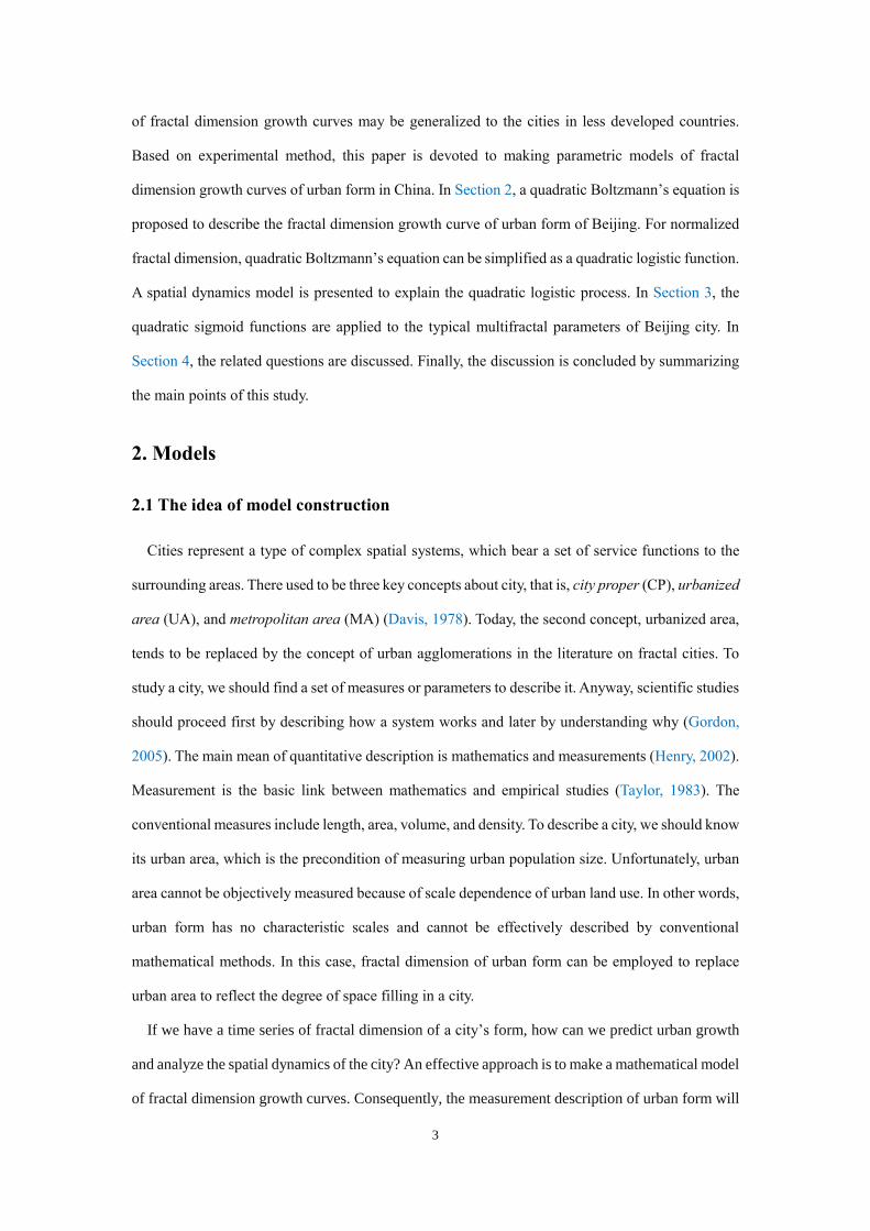
Selection Criterion (1) Statistics: goodness of fit (R2 ); (2) Logic: Dmax≤dE=2.
Function Models’ uses (1) Predict urban growth; (2) Explain urban evolution; (3)
Sharpen urban questions
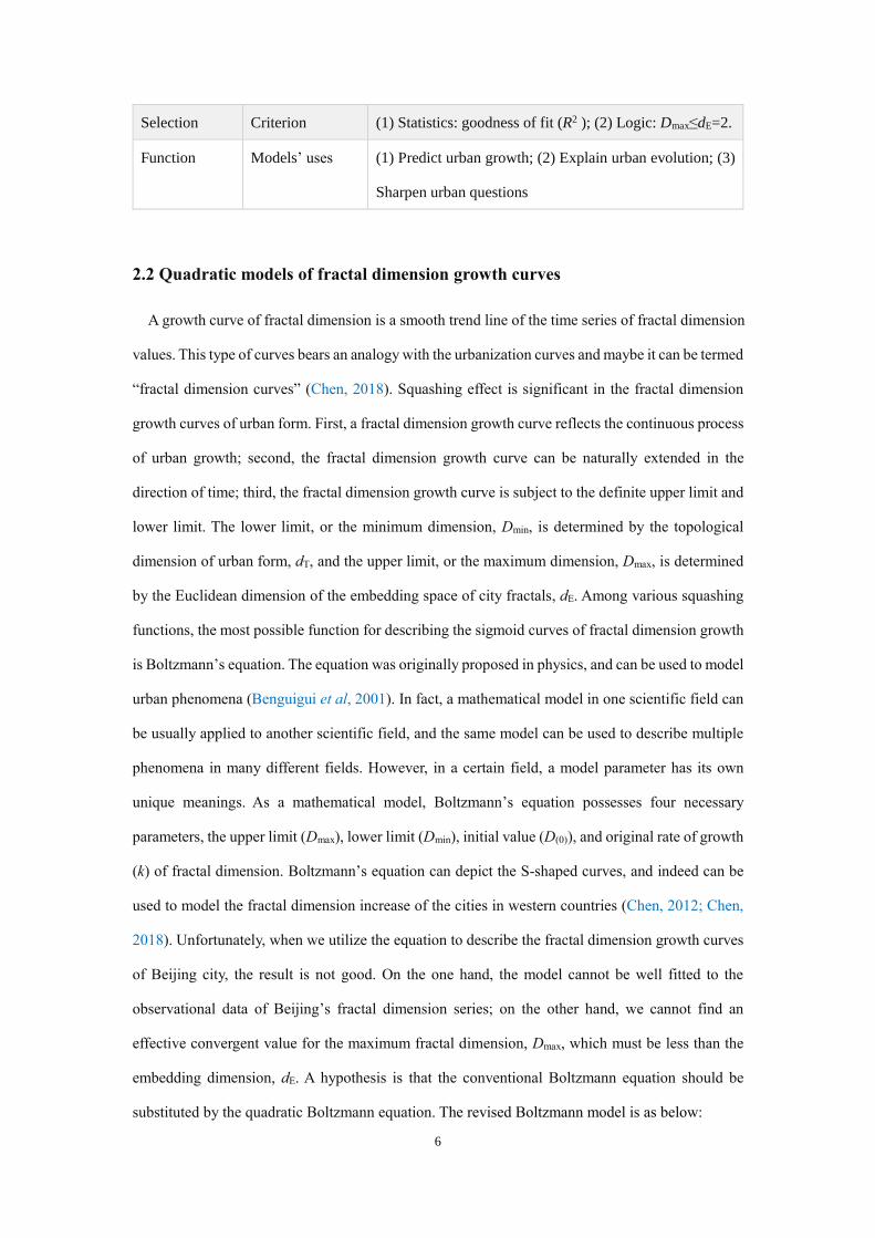
2.2 Quadratic models of fractal dimension growth curves
A growth curve of fractal dimension is a smooth trend line of the time series of fractal dimension
values. This type of curves bears an analogy with the urbanization curves and maybe it can be termed
“fractal dimension curves” (Chen, 2018). Squashing effect is significant in the fractal dimension
growth curves of urban form. First, a fractal dimension growth curve reflects the continuous process
of urban growth; second, the fractal dimension growth curve can be naturally extended in the
direction of time; third, the fractal dimension growth curve is subject to the definite upper limit and
lower limit. The lower limit, or the minimum dimension, Dmin, is determined by the topological
dimension of urban form, dT, and the upper limit, or the maximum dimension, Dmax, is determined
by the Euclidean dimension of the embedding space of city fractals, dE. Among various squashing
functions, the most possible function for describing the sigmoid curves of fractal dimension growth
is Boltzmann’s equation. The equation was originally proposed in physics, and can be used to model
urban phenomena (Benguigui et al, 2001). In fact, a mathematical model in one scientific field can
be usually applied to another scientific field, and the same model can be used to describe multiple
phenomena in many different fields. However, in a certain field, a model parameter has its own
unique meanings. As a mathematical model, Boltzmann’s equation possesses four necessary
parameters, the upper limit (Dmax), lower limit (Dmin), initial value (D(0)), and original rate of growth
(k) of fractal dimension. Boltzmann’s equation can depict the S-shaped curves, and indeed can be
used to model the fractal dimension increase of the cities in western countries (Chen, 2012; Chen,
2018). Unfortunately, when we utilize the equation to describe the fractal dimension growth curves
of Beijing city, the result is not good. On the one hand, the model cannot be well fitted to the
observational data of Beijing’s fractal dimension series; on the other hand, we cannot find an
effective convergent value for the maximum fractal dimension, Dmax, which must be less than the
embedding dimension, dE. A hypothesis is that the conventional Boltzmann equation should be
substituted by the quadratic Boltzmann equation. The revised Boltzmann model is as below:

7
2
max min max minmin min 2 2
max (0) ( ) 0
2
(0) min
( )
1 [ ] 1 exp( )kt
D D D DD t D D
D D t te
D D p
, (1)
in which D(t) denotes the fractal dimension of urban form in time of t, D(0) is the fractal dimension
in the initial time, Dmax≤dE refers to the upper limit of fractal dimension, Dmin≥dT refers to the lower
limit of fractal dimension, k is the inherent growth rate, p is the temporal scaling parameter, and t0,
a temporal translational scale parameter indicating a critical time scale. The scale and scaling
parameters can be respectively expressed as p=1/k and t0=p[ln((Dmax-D(0))/(D(0)-Dmin))]1/2. For the
normalized fractal dimension, equation (1) can be reduced to a quadratic logistic function
2)(*
)0(minmax
min*
)1/1(1
1)()(
kteDDD
DtDtD
, (2)
where D*(t) denotes the fractal dimension normalized by the range, and D(0)*=(D(0)-Dmin)/ (Dmax-
Dmin) indicates the normalized result of the original fractal dimension value, D(0). The fractal
dimension range is the difference between the maximum dimension and the minimum dimension,
i.e., Dmax-Dmin. In theory, we have Dmax=dE=2 and Dmin= dT=0 (Thomas et al, 2007). In practice,
however, the numerical ranges of parameters are 1< Dmax≤dE=2 and dT=0≤Dmin≤1. In fact, the box-
counting method can be employed to estimate the fractal dimension values of urban form. There are
two approaches to making use of the box-counting method. One is the method of fixed maximum
box based on constant study area, and the other is that of unfixed maximum box based on variable
study area. For the former case, fractal dimension values come between 0 and 2; while for the latter
case, fractal dimension values vary from 1 to 2 (Chen, 2012).
The model of the 1-dimensional dynamics can be derived from the logistic model of the fractional
dimension growth curves of urban form. The derivative of equation (2) is a quadratic logistic
equation
)](1)[(2d
)(d **2*
tDttDkt
tD , (3)
which reflects the growth rate of fractal dimension. Without loss of generality, the time interval can
be set as Δt=1. Thus, equation (3) can be discretized to yield a 1-dimensional map such as
2*2*2*
1 2)21( ttt tDkDtkD . (4)
Using equation (4), we can generate a time series of fractal dimension for urban form, which is

8
consistent with the values predicted by equation (2). For the comparability of fractal dimension
values, the same maximum box can be applied to different study areas in different years. In this case,
the minimum dimension value of growing city fractals can be treated as Dmin=dT=0 in theory. Thus,
equation (1) can be reduced to
2
max
( )
max (0)
( )1 ( / 1) kt
DD t
D D e
, (5)
which is a quadratic logistic function (Chen, 2016). The normalized fractal dimension can be
simplified as Dt*=D(t)/Dmax. Accordingly, equation (4) can be rewritten as
22 2
1
max
2(1 2 )t t t
k tD k t D D
D , (6)
which is equivalent to equation (4) but can be used to simulate fractal dimension growth. In other
words, equation (6) is a 1-dimensional map based on quadratic logistic function and non-normalized
fractal dimension. This map differs from the well-known logistic map, which can generate complex
dynamics such as periodic oscillations and chaos (May, 1976). The corresponding differential
equation of equation (6) is as follows
2
max
d ( ) ( )2 ( )[1 ]
d
D t D tk tD t
t D , (7)
which is equivalent to equation (3) and reflects the velocity of fractal dimension growth. It is easy
to demonstrate that equation (5) is just the special solution to equation (7). In other words, equation
(5) is a quadratic logistic equation of fractal dimension growth curves of urban form.
2.3 Tentative derivation of quadratic logistic model
In the studies on fractal cities, fractal dimension as a characteristic parameter of scale-free
distributions is actually a substitute of urban area, which is a scale-dependent measure. In order to
derive the parametric models of fractal dimension growth curves of urban form, we should define a
set of measurements of cities which can be used to link fractal dimension to urban area (Appendix
1). In theory, a region can divided into urban places and rural places. However, there is no clear
boundaries between urban land and rural land. If we define a study area around a city, urban land
and rural land are interlaced with each other. Consequently, urban places and rural places form
complicated patterns and cascade structure, which can be described with multifractal scaling (Chen,

9
2016). For the convenience of description and measurement, we should substitute the concepts of
space-filled place and space-saved place for the notions of urban place and rural place (Chen, 2012).
The logistic function of fractal dimension growth is a spatial replacement equation that represents
the progressive replacement of natural areas by urban and rural built-up areas in the course of time
(Chen2014a). On the base of Boltzmann’s equation of fractal dimension growth, a spatial
replacement index has been defined by means of the normalized fractal dimension (Chen, 2012).
The replacement measurement can be further researched in the new framework of quadratic
Boltzmann’s equation. From equation (2), it follows that
2
*
0
*
0
*
*
)()1
ln(])(1
)(ln[ kt
D
D
tD
tD
, (8)
in which 0<D*<1. A spatial filled-unfilled ratio (FUR) of urban growth can be defined as
])exp[(1)(1
)(
)(
)()( 2
*
0
*
0
*
*
ktD
D
tD
tD
tV
tUtO
, (9)
where U denotes the filled extent of urban space (e.g., space-filling area) with various artificial
buildings, which can be measured by the pixel number of built-up land on digital maps, and V, refers
to the unfilled extent of space (e.g., space-saving area), in which there is no constructions or artificial
structures. Thus we have
)(
)(
)()(
)(
1)(
)()(*
tS
tU
tVtU
tU
tO
tOtD
, (10)
where S represents the total space of urbanized region, that is, S=U+V. This indicates that V is the
complementary set of U, and vice versa. The higher the O value is, the higher the extent of space-
filling will be. The normalized fractal dimension can be regarded as level of space filling (SFL) of
cities, indicating the degree of spatial replacement. It can be employed to estimate the remaining
space of urban growth. The space-filling extent, U, is usually a known number because it can be
measured using digital maps. However, the space-saving area, V, is often unknown (Chen, 2012).
In this case, the unfilled space of an urban region can be estimated by fractal dimension values.
From equation (9) it follows
)1)(
1)(()(
*
tDtUtV . (11)
This implies that the space-saving extent can be figured out by means of normalized fractal

10
dimension and space-filling area. The sum of space-filling extent and space-saving extent gives the
total spatial area of a fractal city, that is
)(
)()()()(
* tD
tUtVtUtS , (12)
which is equivalent to equation (10). Equations (11) and (12) suggest a set of spatial measurements
of urban growth and form (Appendix 1).
The space-filling extent and space-saving extent are both dynamic quantities. However, the total
space area of a city can be treated in two different ways. One is a dynamic way, and the other, a
static way. Equation (12) shows a dynamic concept for urban total space, which changes over time.
In fact, a city cannot grow without any limits. There exists an ultimate spatial sphere for urban
expansion. The greatest extreme of urban space can be termed spatial capacity of a city. Urban land
use can be modeled with logistic function or quadratic logistic function (Chen, 2014b). Thus the
spatial capacity of urban growth can be estimated by general logistic models. In other words, the
capacity parameter of a logistic model or a quadratic logistic model can serve for the static total
quantity of urban space. The fractal dimension series of a city’s form can be estimated based on
either fixed study area or variable study area. Based on a variable study area, the total space of urban
growth can be treated as a dynamic concept; while based on the fixed study area, the urban total
space should be treated as a static quantity measured by a spatial capacity parameter.
To derive the models of fractal dimension growth curves, we can make a model of 2-dimensional
spatial dynamics. The process of urban growth is a nonlinear dynamic process of urban space filling
and replacement. Suppose that an urban region is divided into two types: one is filled space, and the
other, unfilled space. The former can measured by space-filling extent, U(t), while the latter can be
measured by space-saving extent, V(t). Thus, the interaction between filled space (used space) and
unfilled space (remaining space) can be described with two differential equations
])()(
)()()([
d
)(d
tVtU
tVtUtUt
t
tU
, (13)
])()(
)()()([
d
)(d
tVtU
tVtUtVt
t
tV
, (14)
where α, β, and λ are three parameters. This implies that the growth rate of filled space, dU(t)/dt, is
proportional to the size of filled space, U(t), and the coupling interaction between filled and unfilled

11
space, but not directly related to unfilled space size; the growth rate of unfilled space, dV(t)/dt, is
proportional to the size of unfilled space, V(t), and the coupling action between filled and unfilled
space, but not directly related to filled space size. The growth of unfilled space proceeds from natural
land, rural area, old city transformation, counter urbanization, and so on. Differing from the spatial
replacement of the cities in western developed countries (Chen, 2012), both dU(t)/dt and dV(t)/dt
here are proportional to the product of time t and U(t) or V(t) and the product of t and
U(t)V(t)/(U(t)+V(t)). From equations (13) and (14), we can derive equation (3). In fact, taking
derivative of equation (10), we have
t
tV
t
tU
tVtU
tU
tVtU
ttU
t
tD
d
)(d
d
)(d
)]()([
)(
)()(
d/)(d
d
)(d2
*
. (15)
Substituting equations (13) and (14) into equation (15) yields
))()(
)(
)()(
)((
)()(
)(
)]()([
)()(
d
)(d2
*
tVtU
tV
tVtU
tU
tVtU
tU
tVtU
tVtU
tt
tD
. (16)
According to equation (10), D*=U/(U+V), 1-D*=V/(U+V). So equation (16) can be expressed as
)](1)[()(d
)(d ***
tDttDt
tD . (17)
Comparing equations (17) with equation (3) shows
22k . (18)
This indicates that equations (13) and (14) are mathematically equivalent to equation (3). The
dynamical analysis based on the 1-dimensional logistic equation can be associated with the
dynamical analysis based on the 2-dimensional space replacement model. Discretizing equations
(13) and (14) yields a 2-dimensional map as below
)(1
tt
ttttt
VU
VUUtUU
, (19)
)(1
tt
ttttt
VU
VUVtVV
, (20)
where Ut and Vt are the discrete expressions of U(t) and V(t), respectively. This suggests that a 1-
dimensional map, equation (4), can be converted into a 2-dimensional map, equations (19) and (20).
Using equations (19) and (20), we can generate a time series of approximate fractal dimension of

12
urban growth, which is consistent with the values created by equation (4). By developing the
expression of 2-dimensional spatial dynamic equations, we can further derive the quadratic
Boltzmann equation of fractal dimension growth curves in this similar way.

13
Figure 1 Eight representative images reflecting the growth and morphology of Beijing city (1984-
2009)
Note: The urban a boundaries are delineated by using CCA (Rozenfeld et al, 2008; Rozenfeld et al, 2011).
3. Empirical analysis
3.1 Study area and methods
The effect of the models can be testified by the observational data of fractal dimension of urban
form. The purpose of modeling is insight—polarizing thinking and sharpening questions--rather
than number (Hamming, 1962; Karlin, 1983). However, the academic progress of our understanding
the world relies heavily on the interplay of quantifiable data with models (Louf and Barthelemy,
2014). Therefore, before discussing the insight from a research, we must examine the goodness of
fit of the models to the observed data by statistical analysis, and further, we should check the logic
consistency between models and data by numerical analysis. The city of Beijing can be taken as an
example to make an empirical analysis and numerical experiment. Beijing is a typical megacity with
urban population more than 15 million inside the metropolitan area in 2010 (the sixth census year).
The multifractal parameters of urban form can be calculated through remote sensing images for 13
years between 1984 and 2009. In fact, a number of remote sensing images of Beijing from National
Aeronautics and Space Administration (NASA) are available for spatial analysis. The ground
resolution of these images is 30 meters. The detailed information about these images has been
clarified in previous work (Chen and Wang, 2013). The urban agglomeration of Beijing takes on
complicated and irregular spatial patterns (Figure 1). The multifractal features and properties of

14
Beijing’s urban form have been illustrated and demonstrated (Chen and Wang, 2013; Huang and
Chen, 2018). If we obtain a sample path of fractal dimension of urban growth in different years, the
quadratic sigmoid functions can be fitted to the fractal dimension data to verify the models. Then,
the modeling result can be applied to analyzing Beijing’s urban growth and form.
The ArcGIS technology is employed to extract spatial data from remote sensing images, and
Matlab-based computer programming is used to calculate multifractal parameters. The analytical
process is as follows. The first step is to define an urban boundary for each year. The urban
boundary is termed urban envelope (Batty and Longley, 1994; Longley et al, 1991). Several
effective approaches to identifying urban boundaries have been developed recent years (Jiang and
Jia, 2011; Rozenfeld et al, 2011; Tannier et al, 2011). In this paper, the “City Clustering Algorithm”
(CCA) developed by Rozenfeld et al (2008, 2011) is employed to delineate the boundaries of
Beijing’s urban agglomeration in different years. By the urban envelope, we can compute urbanized
area and estimate city size. The second step is to define a study area for fractal dimension
measurement. As indicated above, there are two ways of determining study region for fractal
dimension measurement (Chen, 2012). One is to fix the study area for all years of images (Batty
and Longley, 1994; Chen and Wang, 2013; Shen, 2002), and the other is to select variable study area
according to city size and urbanized area (Benguigui et al, 2000; Feng and Chen, 2010). In this
study, for comparability, we define a fixed study area for the 13 years according to the urban
envelope in the last year (2009). The third step is to extract spatial data using box-counting
method. The functional box-counting method can be used to extract spatial data and calculate fractal
dimension. This method is proposed by Lovejoy et al (1987) and consolidated by Chen (1995). It is
an efficient approach to estimating fractal parameters of urban form and urban systems (Chen, 2014c;
Chen and Wang, 2013; Feng and Chen, 2010; Huang and Chen, 2018). The fixed largest box is
applied to the urban images in different years. Based on the maximum box, a hierarchy of functional
boxes can be generated by the rule of spatial subdivision (Chen and Wang, 2013). The fourth step
is to calculate multifractal parameters using the least squares method. By means of least
squares calculation, we can determine the f(α) singularity spectrum using the approach developed
by Chhabra and Jensen (1989) and Chhabra et al (1989). In order to guarantee proper multifractal
spectrums, the intercepts of logarithmic linear regression models based on fractal relations are fixed
to zero (Huang and Chen, 2018). Then, by Legendre’s transform, we can reckon the generalized

15
correlation dimension Dq. In the global multifractal dimension spectrum, capacity dimension (D0),
information dimension (D1), and correlation dimension (D2) represent three typical parameters of
multi-scaling fractal form. The three parameters will be employed to verify the models for fractal
dimension growth curves (Table 2).
It is necessary to clarify two problems involved with data extraction and parameter estimation.
First, the quality of remoted sensing images influences fractal dimension measurement. Among the
13 years of images, only three Landsat TM images and two Landsat ETM+ images are most
appropriate for fractal study because these images were chiefly taken in autumn or winter, in which
there is less obstruction from clouds and plants (Chen and Wang, 2013). In order to extend the
sample path of the time series of fractal dimension, we make use of all the 13 years of images we
could get. The quality difference in different years causes fluctuation of fractal dimension values
and urban area values. However, the random fluctuation results in variability instead of bias because
positive and negative errors always counteract each other. Second, CCA is essentially a spatial
search method based on spatial cluster, and different searching radius (distance threshold) results in
different urban boundaries. Larger searching radius leads to larger study area. In this study, the
searching radius is set as 1000 meters according to the idea from characteristic scales, which will
be clarified in a companion paper. Fortunately, the two problems have impact on parameter
estimation, but have no significant influence on the model expressions and statistic inference.
Table 2 Three typical multifractal parameters of Beijing’s urban form and the corresponding
urban area (1984-2009)
Year Fractal dimension Urban area
A Capacity dimension
D0
Information dimension
D1
Correlation dimension
D2
1984 1.4994 1.3961 1.3553 393.3022
1988 1.5091 1.4234 1.3935 538.0889
1989 1.5374 1.4467 1.4105 530.2158
1991 1.5645 1.4726 1.4392 644.8084
1992 1.5849 1.5078 1.4797 729.0497
1994 1.5944 1.5213 1.4920 867.1342
1995 1.6522 1.5707 1.5373 1032.6239
1996 1.6789 1.5934 1.5560 1073.5342
1998 1.6702 1.5871 1.5531 1087.2600
16
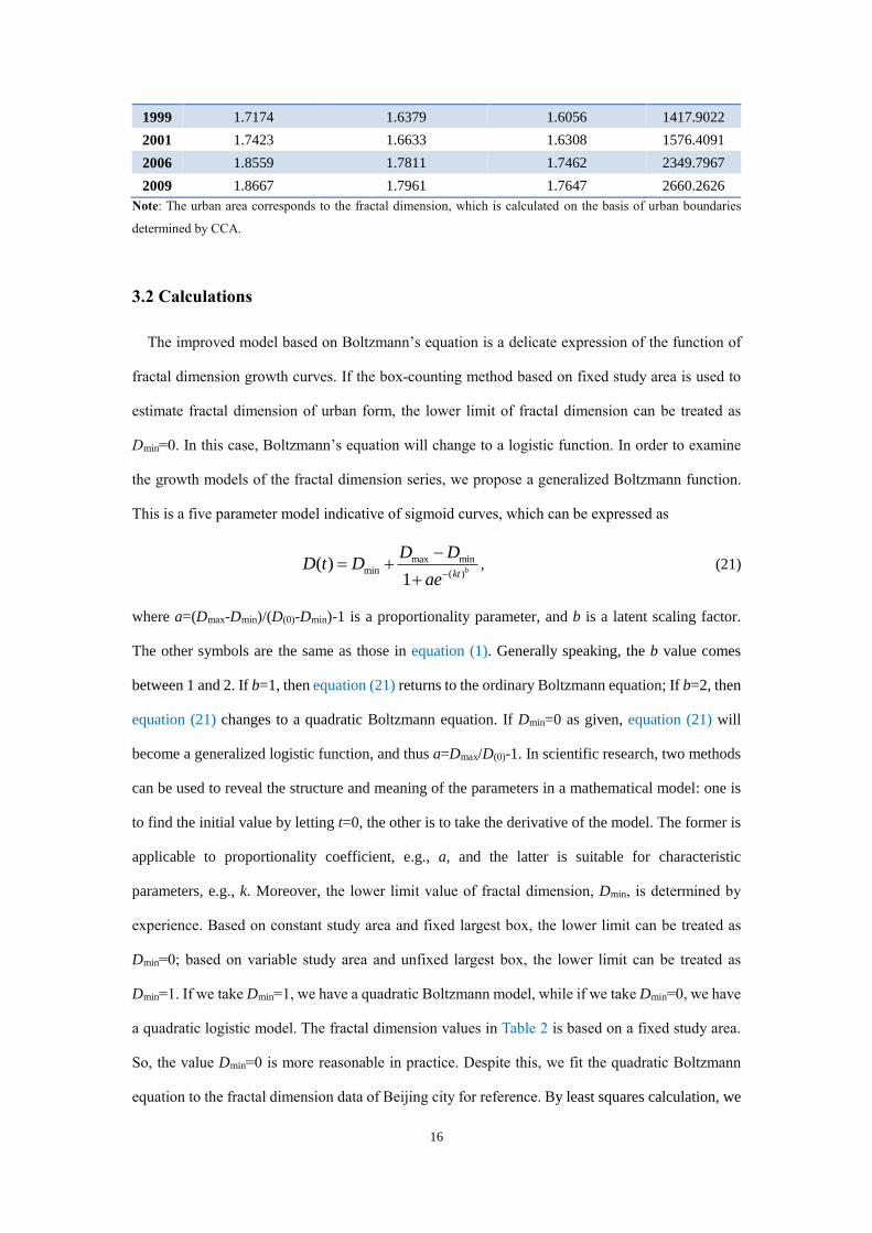
1999 1.7174 1.6379 1.6056 1417.9022
2001 1.7423 1.6633 1.6308 1576.4091
2006 1.8559 1.7811 1.7462 2349.7967
2009 1.8667 1.7961 1.7647 2660.2626
Note: The urban area corresponds to the fractal dimension, which is calculated on the basis of urban boundaries
determined by CCA.
3.2 Calculations
The improved model based on Boltzmann’s equation is a delicate expression of the function of
fractal dimension growth curves. If the box-counting method based on fixed study area is used to
estimate fractal dimension of urban form, the lower limit of fractal dimension can be treated as
Dmin=0. In this case, Boltzmann’s equation will change to a logistic function. In order to examine
the growth models of the fractal dimension series, we propose a generalized Boltzmann function.
This is a five parameter model indicative of sigmoid curves, which can be expressed as
max minmin ( )
( )1
bkt
D DD t D
ae
, (21)
where a=(Dmax-Dmin)/(D(0)-Dmin)-1 is a proportionality parameter, and b is a latent scaling factor.
The other symbols are the same as those in equation (1). Generally speaking, the b value comes
between 1 and 2. If b=1, then equation (21) returns to the ordinary Boltzmann equation; If b=2, then
equation (21) changes to a quadratic Boltzmann equation. If Dmin=0 as given, equation (21) will
become a generalized logistic function, and thus a=Dmax/D(0)-1. In scientific research, two methods
can be used to reveal the structure and meaning of the parameters in a mathematical model: one is
to find the initial value by letting t=0, the other is to take the derivative of the model. The former is
applicable to proportionality coefficient, e.g., a, and the latter is suitable for characteristic
parameters, e.g., k. Moreover, the lower limit value of fractal dimension, Dmin, is determined by
experience. Based on constant study area and fixed largest box, the lower limit can be treated as
Dmin=0; based on variable study area and unfixed largest box, the lower limit can be treated as
Dmin=1. If we take Dmin=1, we have a quadratic Boltzmann model, while if we take Dmin=0, we have
a quadratic logistic model. The fractal dimension values in Table 2 is based on a fixed study area.
So, the value Dmin=0 is more reasonable in practice. Despite this, we fit the quadratic Boltzmann
equation to the fractal dimension data of Beijing city for reference. By least squares calculation, we
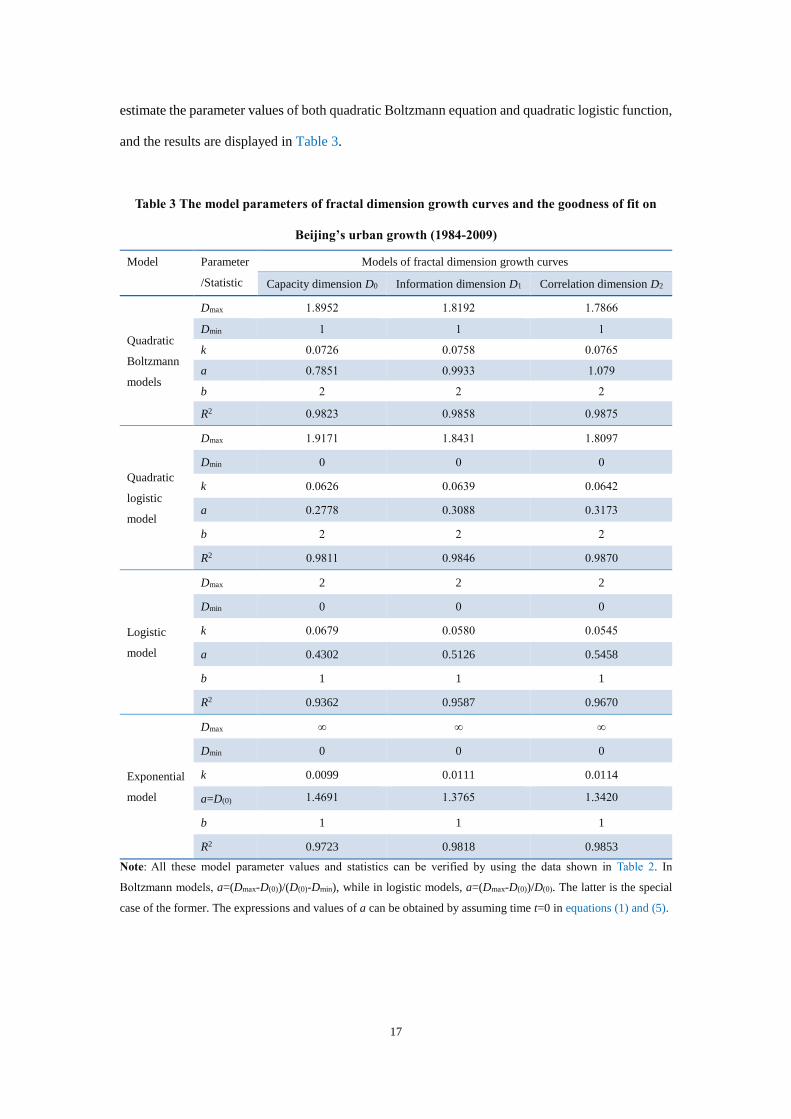
17
estimate the parameter values of both quadratic Boltzmann equation and quadratic logistic function,
and the results are displayed in Table 3.
Table 3 The model parameters of fractal dimension growth curves and the goodness of fit on
Beijing’s urban growth (1984-2009)
Model Parameter
/Statistic
Models of fractal dimension growth curves
Capacity dimension D0 Information dimension D1 Correlation dimension D2
Quadratic
Boltzmann
models
Dmax 1.8952 1.8192 1.7866
Dmin 1 1 1
k 0.0726 0.0758 0.0765
a 0.7851 0.9933 1.079
b 2 2 2
R2 0.9823 0.9858 0.9875
Quadratic
logistic
model
Dmax 1.9171 1.8431 1.8097
Dmin 0 0 0
k 0.0626 0.0639 0.0642
a 0.2778 0.3088 0.3173
b 2 2 2
R2 0.9811 0.9846 0.9870
Logistic
model
Dmax 2 2 2
Dmin 0 0 0
k 0.0679 0.0580 0.0545
a 0.4302 0.5126 0.5458
b 1 1 1
R2 0.9362 0.9587 0.9670
Exponential
model
Dmax ∞ ∞ ∞
Dmin 0 0 0
k 0.0099 0.0111 0.0114
a=D(0) 1.4691 1.3765 1.3420
b 1 1 1
R2 0.9723 0.9818 0.9853
Note: All these model parameter values and statistics can be verified by using the data shown in Table 2. In
Boltzmann models, a=(Dmax-D(0))/(D(0)-Dmin), while in logistic models, a=(Dmax-D(0))/D(0). The latter is the special
case of the former. The expressions and values of a can be obtained by assuming time t=0 in equations (1) and (5).

18
a. Capacity dimension (1.4<D0<2.0)
b. Information dimension (1.3<D1<1.9)
1.4
1.5
1.6
1.7
1.8
1.9
2.0
1980 1985 1990 1995 2000 2005 2010 2015 2020
Cap
acit
y d
imen
sio
n,
D0
Year
Observational value
Predicted value
1.3
1.4
1.5
1.6
1.7
1.8
1.9
1980 1985 1990 1995 2000 2005 2010 2015 2020
Info
rmat
ion
dim
ensi
on
, D
1
Year
Observational value
Predicted value
1.3
1.4
1.5
1.6
1.7
1.8
1.9
1980 1985 1990 1995 2000 2005 2010 2015 2020
Co
rrel
atio
n d
imen
sio
n, D
2
Year
Observational value
Predicted value

19
c. Correlation dimension (1.3<D2<1.9)
Figure 2 Three quadratic logistic curves of fractal dimension growth of Beijing’s urban form
(1984-2020)
Note: The trend lines are generated by using the quadratic logistic models of fractal dimension growth. The
matching effect between the observed values of the fractal dimension of Beijing’s urban form and the
corresponding predicted values based on quadratic Boltzmann’s equation is similar to the these plots.
The mathematical expressions of the quadratic growth models can be given using the above
estimated parameter values. For capacity dimension (q=0), information dimension (q=1), and
correlation dimension (q=2), the quadratic logistic models are as follows
20 (0.0626 )
1.9171ˆ ( )1 0.2778 t
D te
,21 (0.0639 )
1.8431ˆ ( )1 0.3088 t
D te
,22 (0.0642 )
1.8097ˆ ( )1 0.3173 t
D te
.
The goodness of fit are about R2=0.9811, 0.9846, and 0.9870, respectively. The hat “^” indicates
predicted value. For reference, the quadratic Boltzmann models are given as below:
20 (0.0726 )
0.8952ˆ ( ) 1+1 0.7851 t
D te
,21 (0.0758 )
0.8192ˆ ( ) 1+1 0.9933 t
D te
,
22 (0.0765 )
0.7866ˆ ( ) 1+1 1.0790 t
D te
.
The goodness of fit are around R2=0.9823, 0.9858, and 0.9875, respectively. By means of these
models, we can compute the predicted value of the three types of fractal dimension. Based on the
quadratic logistic models, the observed values and the calculated values of fractal dimensions can
be effectively matched (Figure 2). Based on the Boltzmann model, the fitting effect is similar. The
fluctuation of fractal dimension values is owing to the random disturbance proceeding from the
quality of remoted sensing images, as indicated above. As far as the prediction analysis is concerned,
the two models are all acceptable. However, if we consider a longer time scale, we will prefer to the
logistic model. The reason is that, based on the fixed study area, the initial fractal dimension is close
to Dmin=0 instead of Dmin=1 (Shen, 2002).
In order to compare the modeling effect of different functions, we might as well fit the general
logistic model to the observational data of Beijing's fractal dimension values. If we take Dmin=0 and
b=1 in equation (21), we will have an ordinary logistic model of fractal dimension growth curves.
However, the conventional logistic function cannot be well fitted to the observational data of fractal
20
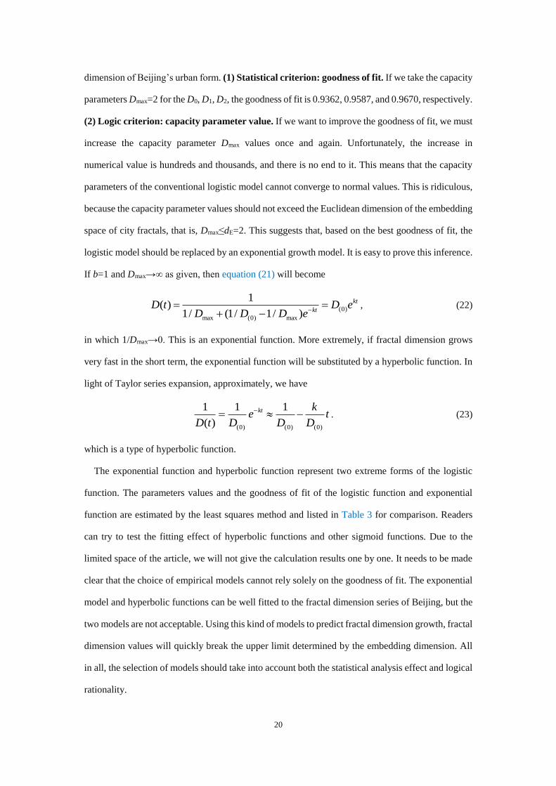
dimension of Beijing’s urban form. (1) Statistical criterion: goodness of fit. If we take the capacity
parameters Dmax=2 for the D0, D1, D2, the goodness of fit is 0.9362, 0.9587, and 0.9670, respectively.
(2) Logic criterion: capacity parameter value. If we want to improve the goodness of fit, we must
increase the capacity parameter Dmax values once and again. Unfortunately, the increase in
numerical value is hundreds and thousands, and there is no end to it. This means that the capacity
parameters of the conventional logistic model cannot converge to normal values. This is ridiculous,
because the capacity parameter values should not exceed the Euclidean dimension of the embedding
space of city fractals, that is, Dmax≤dE=2. This suggests that, based on the best goodness of fit, the
logistic model should be replaced by an exponential growth model. It is easy to prove this inference.
If b=1 and Dmax→∞ as given, then equation (21) will become
(0)
max (0) max
1( )
1/ (1/ 1/ )
kt
ktD t D e
D D D e
, (22)
in which 1/Dmax→0. This is an exponential function. More extremely, if fractal dimension grows
very fast in the short term, the exponential function will be substituted by a hyperbolic function. In
light of Taylor series expansion, approximately, we have
(0) (0) (0)
1 1 1
( )
kt ke t
D t D D D
. (23)
which is a type of hyperbolic function.
The exponential function and hyperbolic function represent two extreme forms of the logistic
function. The parameters values and the goodness of fit of the logistic function and exponential
function are estimated by the least squares method and listed in Table 3 for comparison. Readers
can try to test the fitting effect of hyperbolic functions and other sigmoid functions. Due to the
limited space of the article, we will not give the calculation results one by one. It needs to be made
clear that the choice of empirical models cannot rely solely on the goodness of fit. The exponential
model and hyperbolic functions can be well fitted to the fractal dimension series of Beijing, but the
two models are not acceptable. Using this kind of models to predict fractal dimension growth, fractal
dimension values will quickly break the upper limit determined by the embedding dimension. All
in all, the selection of models should take into account both the statistical analysis effect and logical
rationality.

21
a. Capacity dimension (1.4<D0<2.0)
b. Information dimension (1.3<D1<1.9)
1.4
1.5
1.6
1.7
1.8
1.9
2.0
1980 1985 1990 1995 2000 2005 2010 2015 2020
Cap
acit
y d
imen
sio
n, D
0
Year
Observed value
Iteration result
1.3
1.4
1.5
1.6
1.7
1.8
1.9
1980 1985 1990 1995 2000 2005 2010 2015 2020
Info
rmat
iol
dim
ensi
on
, D
1
Year
Observed value
Iteration result
1.3
1.4
1.5
1.6
1.7
1.8
1.9
1980 1985 1990 1995 2000 2005 2010 2015 2020
Co
rrel
atio
n d
imen
sio
n, D
2
Year
Observed value
Iteration result

22
c. Correlation dimension (1.3<D2<1.9)
Figure 3 Three types of fractal dimension values and the corresponding iteration results using 1-
dimensional map (1984-2020)
Note: The trend lines are generated by using the 1-dimensional quadratic logistic map of fractal dimension growth.
3.3 Numerical iteration analysis
The quadratic logistic map can be utilized to make an analysis of numerical iteration for Beijing’s
urban growth. This iteration is in fact the simplest numerical simulation of fractal dimension growth.
Numerical analysis can testify the modeling effect from the computational angle of view. Equations
(4) and (6) are 1-dimensional maps based on the quadratic logistic function. Equation (6) can be
used to simulate the fractal dimension growth, and equation (4) can be used to simulate the
normalized fractal dimension growth. The two numerical calculation processes are equivalent to
one another, and we just need to investigate one of them. Using a 1-dimensional quadratic logistic
map, we can generate the time series of multifractal parameters of Beijing’s urban form. Suppose
that the initial time is 1984, and time number is t=n-1984, where n=1984, 1985, …, 2020 denotes
year. For capacity dimension, the initial value D(0)= D(1984)=1.4994 (see Table 2), the maximum
value Dmax=1.9171 (see Table 3); For information dimension, the initial value D(0)= D(1984)=1.3961
(see Table 2), the maximum value Dmax=1.8431 (see Table 3); For correlation dimension, the initial
value D(0)= D(1984)=1.3553 (see Table 2), the maximum value Dmax=1.8097 (see Table 3). By means
of mathematical software such as Matlab or even spreadsheet such as MS Excel, we can implement
numerical computations based on equation (6). Partial results are tabulated as below (Table 4). The
iteration results are generally consistent with the observational values of fractal dimension and the
corresponding predicted values of the empirical models (Figure 3).
Table 4 Comparison between observational values of Beijing’s fractal dimension, predicted
values of quadratic logistic models, and calculated values of 1-dimensional quadratic logistic map
Year Capacity dimension Information dimension Correlation dimension
D0 Ḓ0 Ď0 D1 Ḓ1 Ď1 D2 Ḓ2 Ď2
1984 1.4994 1.5003 1.4994 1.3961 1.4082 1.3961 1.3553 1.3737 1.3553
1988 1.5091 1.5204 1.5246 1.4234 1.4295 1.4223 1.3935 1.3952 1.3817
1989 1.5374 1.5313 1.5368 1.4467 1.4412 1.4351 1.4105 1.4069 1.3945

23
1991 1.5645 1.5595 1.5674 1.4726 1.4712 1.4669 1.4392 1.4371 1.4266
1992 1.5849 1.5762 1.5853 1.5078 1.4890 1.4857 1.4797 1.4551 1.4455
1994 1.5944 1.6140 1.6251 1.5213 1.5292 1.5275 1.4920 1.4956 1.4878
1995 1.6522 1.6344 1.6464 1.5707 1.5509 1.5501 1.5373 1.5174 1.5106
1996 1.6789 1.6554 1.6682 1.5934 1.5733 1.5732 1.5560 1.5399 1.5340
1998 1.6702 1.6981 1.7122 1.5871 1.6186 1.6201 1.5531 1.5856 1.5816
1999 1.7174 1.7192 1.7337 1.6379 1.6409 1.6431 1.6056 1.6081 1.6050
2001 1.7423 1.7594 1.7743 1.6633 1.6834 1.6868 1.6308 1.6507 1.6495
2006 1.8559 1.8403 1.8530 1.7811 1.7675 1.7724 1.7462 1.7350 1.7370
2009 1.8667 1.8721 1.8821 1.7961 1.7998 1.8044 1.7647 1.7672 1.7699
Note: D represents observational data, Ḓ represents predicted value of quadratic logistic models, and Ď represents
calculated value of 1-dimensional quadratic logistic map.
The results lend further support to the parametric models presented in Section 2 and empirical
estimated values of the model parameters in Section 3. If the mathematical structure of a model is
wrong, or if the parameter values of the model depart reality significantly, the calculated values will
not keep consistent with the observed values. In this numerical simulation, the model is based on
the quadratic logistic function, the initial values come from the observational data of fractal
dimension, and the maximum fractal dimension values result from the empirical analysis. Besides,
more numerical experiments can be made as follows. First, discretizing the quadratic Boltzmann’s
equation yields another 1-dimensional map of fractal dimension growth. Using this map, we can
implement another numerical simulation. The new computational results are very similar to the
results shown in Figure 3 and Table 4, and thus are no longer displayed here. Second, using the 2-
dimensional maps, equations (19) and (20), we can also carry out a two-variable numerical
experiment to verify the quadratic logistic models of fractal dimension growth curves. The process
is similar to the process of generating urbanization level curves using the 2-dimensional maps based
on the urban-rural interaction model (Chen, 2009).
3.4 Predictions and measurements of urban growth
By means of the models of fractal dimension growth curves, we can predict the peak and velocity
of urban growth. After all, one of the main functions of mathematical model is prediction
(Fotheringham and O'Kelly, 1989; Kac, 1969). The growth rate of fractal dimension values of urban
form reflects the expansion speed of urban land use or the filling speed of urban space, and thus
reflect the speed of urban human activities. For the quadratic logistic model, the growth rate of

24
fractal dimension values can be expressed by equation (7), which is the derivative of equation (5).
Discretizing equation (7) yields a difference equation of fractal dimension growth rate as below:
2
1
max
2 (1 )t tt t t
D DD D k tD
t D
, (24)
in which the time difference is Δt=1. Equation (24) is equivalent to the 1-dimensional quadratic
logistic map, equation (6). Using equation (24), we can generate the three time series of growth rates
of fractal dimension. The parameter k values are shown in Table 2, that is, 0.0626 for capacity
dimension, 0.0639 for information dimension, and 0.0642 for correlation dimension. However, in
practice, we have simpler way to create the time series of growth rates of fractal dimension for
Beijing’s urban form. The first step is to assign parameters to the quadratic logistic models. This
step has been completed in Subsection 3.2. The second step is to calculate the predicted values of
fractal dimensions using the models shown in Subsection 3.2. Partial values are displayed in Table
4. The third step is to compute the difference values of the fractal dimension time series, and the
difference series represents the growth rates of fractal dimension values. The fourth step is to draw
the plots of fractal dimension growth rate. Through these curves of growth rates, we can intuitively
examine the regularity and characteristics of fractal dimension changes of Beijing’s urban form
(Figure 4).
a. Based on quadratic logistic model
0.000
0.005
0.010
0.015
0.020
0.025
1980 1985 1990 1995 2000 2005 2010 2015 2020 2025
Gro
wth
rat
e
Year
Capacity
Information
Correlation
25
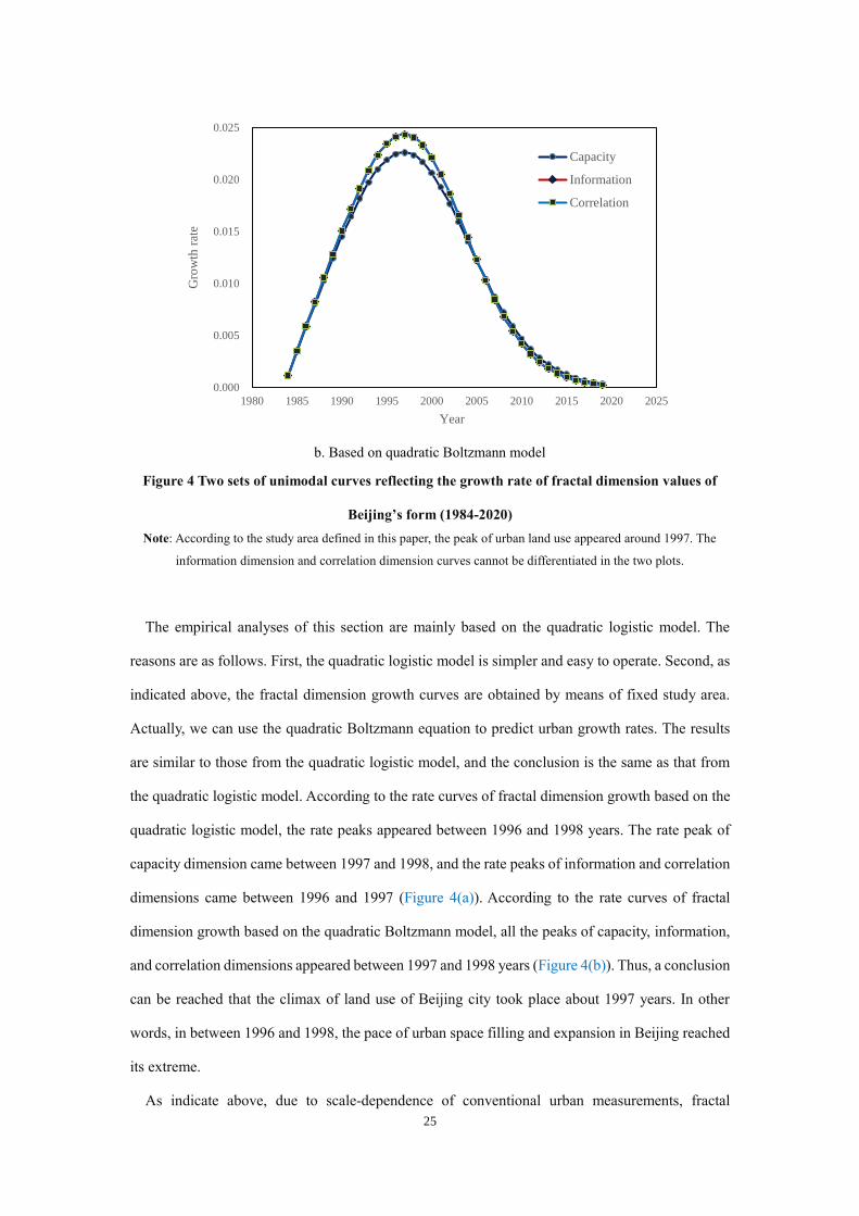
b. Based on quadratic Boltzmann model
Figure 4 Two sets of unimodal curves reflecting the growth rate of fractal dimension values of
Beijing’s form (1984-2020)
Note: According to the study area defined in this paper, the peak of urban land use appeared around 1997. The
information dimension and correlation dimension curves cannot be differentiated in the two plots.
The empirical analyses of this section are mainly based on the quadratic logistic model. The
reasons are as follows. First, the quadratic logistic model is simpler and easy to operate. Second, as
indicated above, the fractal dimension growth curves are obtained by means of fixed study area.
Actually, we can use the quadratic Boltzmann equation to predict urban growth rates. The results
are similar to those from the quadratic logistic model, and the conclusion is the same as that from
the quadratic logistic model. According to the rate curves of fractal dimension growth based on the
quadratic logistic model, the rate peaks appeared between 1996 and 1998 years. The rate peak of
capacity dimension came between 1997 and 1998, and the rate peaks of information and correlation
dimensions came between 1996 and 1997 (Figure 4(a)). According to the rate curves of fractal
dimension growth based on the quadratic Boltzmann model, all the peaks of capacity, information,
and correlation dimensions appeared between 1997 and 1998 years (Figure 4(b)). Thus, a conclusion
can be reached that the climax of land use of Beijing city took place about 1997 years. In other
words, in between 1996 and 1998, the pace of urban space filling and expansion in Beijing reached
its extreme.
As indicate above, due to scale-dependence of conventional urban measurements, fractal
0.000
0.005
0.010
0.015
0.020
0.025
1980 1985 1990 1995 2000 2005 2010 2015 2020 2025
Gro
wth
rat
e
Year
Capacity
Information
Correlation

26
dimension is employed to act as a characteristic parameter of space filling to replace urban area in
urban studies. So far, a recognized method has not been found to determine the urban boundary
objectively. In particular, the fractal dimension values depend on the definition of study area owing
to multifractal property of urban morphology. As a result, for the same city based on different study
area, the rate peak of urban development may appear in different times. Therefore, before making
use of the models of fractal dimension growth curves to predict urban growth, we must make clear
the definition of study region: based on city proper (CP), based on urbanized area (UA), or based
on metropolitan area (MA), and so on.
4. Discussion
Using experiment method, we establish mathematical models of fractal dimension growth curves
of urban form. The basic aim of modeling is to predict the urban growth and explain urban dynamics
in China. The delicate expression of the model is the quadratic Boltzmann equation, while the simple
expression is the quadratic logistic function. We agree the following viewpoint: one of the main
tasks of scientific research is to make models (Neumann, 1961). A model is different from the truth.
A model’s expression of a system is not unique. We can find a better model for a system, but maybe
we will never find the best model for the system. If and only if a model can be derived from one or
a set of postulates by mathematic theory, the model will evolve into a theoretical model from the
empirical model. To derive the quadratic logistic model, we propose a group of spatial measurement
and construct a pair of 2-dimensional dynamic equations. The models are based on Beijing’s fractal
dimension data. However, the results of modeling can be applied to many other Chinese cities.
Setting Dmin=0, Zhao (2017) fitted equation (21) to fractal dimension time series of the 13 main
cities in Beijing, Tianjin, and Hebei region (Jing-Jin-Ji). The results show that the fractal dimension
growth curves of these cities can be described with the various logistic functions: one logistic model
(Baoding city, b≈1), two fractional logistic model (Shijiazhuang and Tianjin, b=1.5), and ten
quadratic logistic model (Beijing, Cangzhou, Chengde, Handan, Hengshui, Langfang, Qinhuangdao,
Tangshan, Xingtai, Zhangjiakou, b=2). All these cities belong to the northern China. A noticeable
discovery is that although the definition of city or study area (e.g., CP, UA, MA) influences fractal
dimension values and model parameter values of fractal dimension growth curves, it has no

27
significant impact on the model’s expression (Table 5). A model’s structure reflect the spatial order
and pattern at the macro level of a system, while the parameter values are often associated with the
interaction between elements at the micro level. Another discovery is that the fractal dimension
growth curves of the cities in the south of China such as Hangzhou, Shenzhen, and Yiwu can be
described with the ordinary logistic function rather than the quadratic logistic function. The reason
may be that, compared with northern Chinese cities, the development of southern Chinese cities is
more significantly acted by the market economy of bottom-up evolution. It is high-level or large-
scale macro factors that determine the mathematical structure of a city’s models, whereas the model
parameters are mainly affected by the micro interaction of urban internal elements.
Table 5 A set of examples of mathematical models of fractal dimension growth curves of Chinese
urban form: logistic function, quadratic logistic function, and fractional logistic function
City Study area Period Data point Mathematical model R2
Beijing Urban
agglomeration
1984-
2009 13 20 (0.0626 )
1.9171ˆ ( )1 0.2778 t
D te
0.9811
Beijing Metropolitan area 1984-
2009 8 20 (0.0572 )
1.8627ˆ ( )1 0.3070 t
D te
0.9955
Jing-Jin-Ji Urban region 1995-
2013 5 20 (0.0292 )
1.5641ˆ ( )1 0.0788 t
D te
0.9783
Shijiazhuang Administrative area 1995-
2013 5 1.50 (0.0370 )
2ˆ ( )1 0.4128 t
D te
0.9428
Tangshan Administrative area 1995-
2013 5 20 (0.0402 )
1.5289ˆ ( )1 0.1246 t
D te
0.9428
Tianjin Administrative area 1995-
2013 5 1.50 (0.0549 )
1.7024ˆ ( )1 0.1257 t
D te
0.9355
Shenzhen Built-up area 1986-
2017 6 0 0.1101
1.8636ˆ ( )1 0.1950 t
D te
0.9844
Note: Jing-Jin-Ji represents the "Beijing Tianjin Hebei region" in the North China Plain. Tianjin, Shijiazhuang,
Tangshan, and Jing-Jin-Ji’s data come from Zhao (2017), Shenzhen’s data come from Ms. Xiaoming Man.
The models of fractal dimension growth curves for the urban form in China are different from
those for the cities in western developed countries and regions. The growth curves of fractal
dimension of European and American urban form can be modeled with the ordinary logistic function
(Chen, 2012; Chen, 2014a; Chen, 2018). Benguigui et al (2000) have published several sets of
fractal dimension time series (1935-1991) of the morphology of the Tel-Aviv metropolis (7-8 years),
and Shen (2002) has presented a fractal dimension time series (1792-1992) of Baltimore’s urban
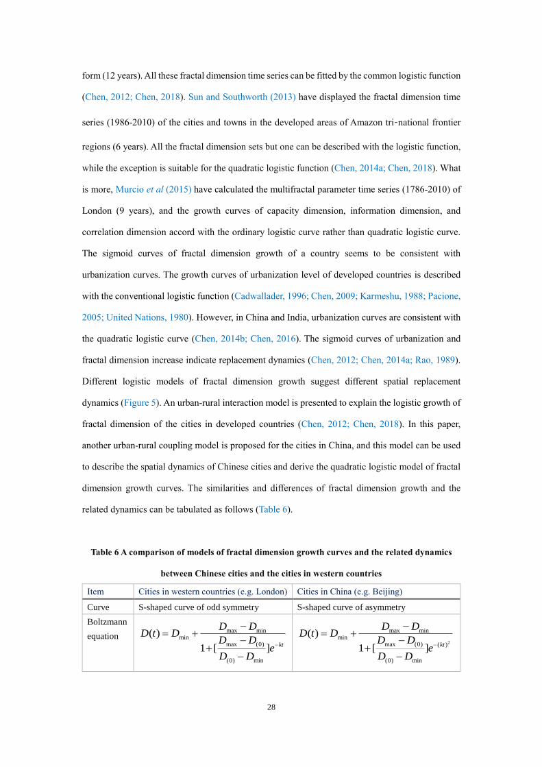
28
form (12 years). All these fractal dimension time series can be fitted by the common logistic function
(Chen, 2012; Chen, 2018). Sun and Southworth (2013) have displayed the fractal dimension time
series (1986-2010) of the cities and towns in the developed areas of Amazon tri‑national frontier
regions (6 years). All the fractal dimension sets but one can be described with the logistic function,
while the exception is suitable for the quadratic logistic function (Chen, 2014a; Chen, 2018). What
is more, Murcio et al (2015) have calculated the multifractal parameter time series (1786-2010) of
London (9 years), and the growth curves of capacity dimension, information dimension, and
correlation dimension accord with the ordinary logistic curve rather than quadratic logistic curve.
The sigmoid curves of fractal dimension growth of a country seems to be consistent with
urbanization curves. The growth curves of urbanization level of developed countries is described
with the conventional logistic function (Cadwallader, 1996; Chen, 2009; Karmeshu, 1988; Pacione,
2005; United Nations, 1980). However, in China and India, urbanization curves are consistent with
the quadratic logistic curve (Chen, 2014b; Chen, 2016). The sigmoid curves of urbanization and
fractal dimension increase indicate replacement dynamics (Chen, 2012; Chen, 2014a; Rao, 1989).
Different logistic models of fractal dimension growth suggest different spatial replacement
dynamics (Figure 5). An urban-rural interaction model is presented to explain the logistic growth of
fractal dimension of the cities in developed countries (Chen, 2012; Chen, 2018). In this paper,
another urban-rural coupling model is proposed for the cities in China, and this model can be used
to describe the spatial dynamics of Chinese cities and derive the quadratic logistic model of fractal
dimension growth curves. The similarities and differences of fractal dimension growth and the
related dynamics can be tabulated as follows (Table 6).
Table 6 A comparison of models of fractal dimension growth curves and the related dynamics
between Chinese cities and the cities in western countries
Item Cities in western countries (e.g. London) Cities in China (e.g. Beijing)
Curve S-shaped curve of odd symmetry S-shaped curve of asymmetry
Boltzmann
equation max min
minmax (0)
(0) min
( )
1 [ ] kt
D DD t D
D De
D D
2
max minmin
max (0) ( )
(0) min
( )
1 [ ] kt
D DD t D
D De
D D

29
Standard
growth
model
*
*
(0)
1( )
1 (1/ 1) ktD t
D e
2
*
* ( )
(0)
1( )
1 (1/ 1) ktD t
D e
General
growth
model
max
max (0)
( )1 ( / 1) kt
DD t
D D e
2
max
( )
max (0)
( )1 ( / 1) kt
DD t
D D e
1-D
dynamic
model max
d ( ) ( )( )[1 ]
d
D t D tkD t
t D
2
max
d ( ) ( )2 ( )[1 ]
d
D t D tk tD t
t D
2-D
dynamic
model
d ( ) ( ) ( )( )
d ( ) ( )
d ( ) ( ) ( )( )
d ( ) ( )
U t U t V tU t
t U t V t
V t U t V tV t
t U t V t
d ( ) ( ) ( )[ ( ) ]
d ( ) ( )
d ( ) ( ) ( )[ ( ) ]
d ( ) ( )
U t U t V tt U t
t U t V t
V t U t V tt V t
t U t V t
Social
mechanism
Process of bottom up urban evolution
under top down rules (self-organized
cities)
Interweaved processes of top down
development and bottom up evolution of
cities (limited self-organized cities)
Note: The standard growth model is based on standardized fractal dimension values, while the general growth model
is based on normal fractal dimension values. The 1-D dynamic models give the growth rates of fractal dimension of
urban form and can be termed growth velocity models of fractal dimension.
Figure 5 Two types of fractal dimension growth curves of urban form: logistic curve and
quadratic logistic curve
Note: The logistic curve is based on London’s model (Chen, 2018), while the quadratic logistic curve is based on
Beijing’s model. The former is a standard S-shaped curve of odd symmetry, while the latter is an S-shaped curve of
asymmetry. The different curves suggests different types of spatial dynamics based on different social conditions.
The distinction between the models of the cities in western countries and those in China lies in
0.00
0.25
0.50
0.75
1.00
1.25
1.50
1.75
2.00
0 25 50 75 100 125 150 175 200
Fra
ctal
dim
ensi
on
D(t
)
Time t
Logistic curve
Quadratic logistic curve

30
latent scaling parameter value. The mathematical forms of the models presented in this paper look
like the expressions put forward in a previous paper (see Chen, 2012). However, the essence is
different. The previous models are common sigmoid functions (the scaling parameter is 1) for
describing the fractal dimension growth curves of urban form in developed countries. In contrast,
this work is to develop quadratic sigmoid function (the scaling parameter is 2) for characterizing
the fractal dimension change of urban growth in China. Sometimes, the latent scaling exponent
comes between 1 and 2. The models of spatial dynamics are significantly distinct from one another.
For the previous model, the rates of growth of filled and unfilled space are independent of time, i.e.,
there is no dominant time factor on the right side of the equal signs of dynamic equations. However,
in the new model, the growth rates of filled and unfilled space depend directly on time.
Fractal dimension is a substitute of urban area, and fractal dimension values reflect the expansion
of urban agglomerations and space filling of urbanized area. According to the law of allometric
growth of urban size and shape, urban area extension is correlated with population size growth.
Population is one the central variables in the study of spatial dynamics of city development
(Dendrinos, 1992), and it represent the first dynamics of urban evolution (Arbesman, 2012). Urban
population activities are imprinted onto the form of urban land use, and what we measure and
calculate is the fractal dimension of urban land use. Generally speaking, there is an allometric
scaling relation between urban area and the corresponding population size (Batty and Longley, 1994;
Chen, 2014b; Lee, 1989; Longley et al, 1991). Where Beijing is concerned, the urban area shown
in Table 1 can be approximately modeled using the quadratic logistic function as below
2(0.0817 )
2847.8631ˆ( )1 4.8828 t
A te
.
The goodness of fit is about R2=0.9886. Strictly, the more advisable scaling exponent for urban area
model is b=3/2, thus we have fractional logistic model rather than a quadratic logistic model. The
parameter values are as follows Amax=3213.7225, a=6.6329, k=0.0914. The goodness of fit is about
R2=0.9923. For simplicity and comparability, the latent scaling factor is approximated as 2.
Accordingly, the population size growth of Beijing city can also be fitted using the quadratic logistic
model (Appendix 2). However, if we examine the data of Beijing’s urban population data, we will
find that the better model is the hyperbolic function rather than the generalized logistic function.
The hyperbolic model is in expression similar to equation (23). The hyperbolic growth model

31
suggests that Beijing's population growth is very fast and lacks effective environmental constraints.
Fast population urbanization leads to a rapid increase in fractal dimension values.
The main shortcomings of this study are as below. First, only one Chinese city is examined in
detail. If we investigate more cities in developing countries, we may find more problems for studies
in next step. Second, the relationships between fractal dimension and the measurements of space-
filled extents in urban and rural regions are not brought to light. The more effective measurements
for urban and rural space may be spatial entropy, which will be studied in a companion paper. Third,
the numerical calculations based on the 2-dimensional map are not fulfilled. Owing to absence of
urban and rural space-filling measurements, the numerical simulation of fractal dimension growth
cannot be implemented by the discrete form of nonlinear coupling equations.
5. Conclusions
The first type of prediction models of fractal dimension growth include Boltzmann equation and
logistic function. This work is devoted to making the second type of parametric models of growth
curves of fractal dimension of urban form by means of experimental method. Using this type of
models, we can predict the fractal dimension growth of many Chinese cities. Based on the
theoretical modeling, empirical analysis, and discussion of questions, the main conclusions of this
study can be reached as follows. First, the fractal dimension growth curve of urban form in
China can be modeled by quadratic Boltzmann’s equation. If a fractal dimension time series is
normalized, the quadratic Boltzmann’s equation will change to a quadratic logistic function. Both
the quadratic Boltzmann’s equation and quadratic logistic function belong to the family of quadratic
sigmoid functions. For simplicity, the quadratic logistic function can be used to approximately
describe the sample path of the fractal dimension series values that is not normalized in practice.
Second, the quadratic logistic functions of the fractal dimension growth curves of urban form
can be derived from the equations of 2-dimensional spatial dynamics. If urban space is divided
into two parts: filled space (used space) and unfilled space (remaining space), we can build a spatial
interaction model of the two types of geographical space. The model can be formulated as two
differential equations indicative of spatial dynamics of urban evolution. From the pair of differential
equations, we can deduce the sigmoid functions of urban fractal dimension growth curves. Third,
32
the models of the urban growth and form in China are the same in structure as the related
models of the cities in western countries, but the model parameter values are different in
essence. As far as the mathematical expressions are concerned, the models of fractal dimension
growth curves of Chinese cities are very similar to those of western cities. However, where model
parameter values are concerned, there is significant difference. The temporal scaling exponent in
the models of the fractal dimension growth curves of the cities in western countries is 1, while the
scaling exponent value of Chinese cities are greater than 1 and often close to 2. The difference of
parameter values reflects the distinction of dynamic mechanism at the micro level. The time factor
is much more significant in the evolution of Chinese cities than in the urban evolution of western
developed countries. Differences in time scaling factor values reflect differences in social and
economic management systems between China and the western countries.
Acknowledgements
This research was sponsored by the National Natural Science Foundations of China (Grant No.
41590843 & 41671167). The supports are gratefully acknowledged. We are very grateful to five
anonymous reviewers whose constructive suggestions were helpful in improving the paper’s quality.
References
Allen PM (1997). Cities and Regions as Self-Organizing Systems: Models of Complexity. London & New
York: Routledge
Arbesman S (2012). The Half-Life of Facts: Why Everything We Know Has An Expiration Date. New
York: Penguin Group.
Batty M, Longley PA (1994). Fractal Cities: A Geometry of Form and Function. London: Academic
Press
Benguigui L, Czamanski D, Marinov M (2001). City growth as a leap-frogging process: an application
to the Tel-Aviv metropolis. Urban Studies, 38(10): 1819-1839
Benguigui L, Czamanski D, Marinov M, Portugali J (2000). When and where is a city fractal?
Environment and Planning B: Planning and Design, 27(4): 507–519
Cadwallader MT (1996). Urban Geography: An Analytical Approach. Upper Saddle River, NJ: Prentice
Hall

33
Chen T (1995). Studies on Fractal Systems of Cities and Towns in the Central Plains of China (Master's
Degree Thesis). Changchun: Department of Geography, Northeast Normal University (in Chinese)
Chen YG (2009). Spatial interaction creates period-doubling bifurcation and chaos of urbanization.
Chaos, Soliton & Fractals, 42(3): 1316-1325
Chen YG (2012). Fractal dimension evolution and spatial replacement dynamics of urban growth. Chaos,
Solitons & Fractals, 45 (2): 115–124
Chen YG (2014a). Urban chaos and replacement dynamics in nature and society. Physica A: Statistical
Mechanics and its Applications, 413: 373-384
Chen YG (2014b). An allometric scaling relation based on logistic growth of cities. Chaos, Solitons &
Fractals, 65: 65-77
Chen YG (2014c). Multifractals of central place systems: models, dimension spectrums, and empirical
analysis. Physica A: Statistical Mechanics and its Applications, 402: 266-282
Chen YG (2016). Defining urban and rural regions by multifractal spectrums of urbanization. Fractals,
24(1): 1650004
Chen YG (2018). Logistic models of fractal dimension growth of urban morphology. Fractals, 26(1):
1850033
Chen YG, Wang JJ (2013). Multifractal characterization of urban form and growth: the case of Beijing.
Environment and Planning B: Planning and Design, 40(5):884-904
Chhabra A, Jensen RV (1989). Direct determination of the f(α) singularity spectrum. Physical Review
Letters, 62(12): 1327-1330
Chhabra A, Meneveau C, Jensen RV, Sreenivasan KR (1989). Direct determination of the f(α) singularity
spectrum and its application to fully developed turbulence. Physical Review A, 40(9): 5284-5294
Davis K (1978). World urbanization: 1950-1970. In: I.S. Bourne, J.W. Simons (eds). Systems of Cities:
Readings on Structure, Growth, and Policy. New York: Oxford University Press, pp92-100
Dendrinos DS (1992). The Dynamics of Cities: Ecological Determinism, Dualism and Chaos. London
and New York: Routledge
Feng J, Chen YG (2010). Spatiotemporal evolution of urban form and land use structure in Hangzhou,
China: evidence from fractals. Environment and Planning B: Planning and Design, 37(5): 838- 856
Fotheringham AS, O'Kelly ME (1989). Spatial Interaction Models: Formulations and Applications.
Boston: Kluwer Academic Publishers
34
Frankhauser P (1994). La Fractalité des Structures Urbaines (The Fractal Aspects of Urban Structures).
Paris: Economica
Gordon K (2005). The mysteries of mass. Scientific American, 293(1):40-46/48
Hamming RW (1962). Numerical Methods for Scientists and Engineers. New York: McGraw-Haw Henry
J (2002). The Scientific Revolution and the Origins of Modern Science (2nd Edition). New York:
Palgrave
Huang LS, Chen YG (2018). A comparison between two OLS-based approaches to estimating urban
multifractal parameters. Fractals, 26(1): 1850019
Jiang B, Jia T (2011). Zipf's law for all the natural cities in the United States: a geospatial perspective.
International Journal of Geographical Information Science, 25(8): 1269-1281
Kac M (1969). Some mathematical models in science. Science, 166: 695-699
Karlin S (1983). Eleventh RA Fischer Memorial Lecture. Royal Society [20 April 1983]
Karmeshu (1988). Demographic models of urbanization. Environment and Planning B: Planning and
Design, 15(1): 47-54
Knox PL, Marston SA (2009). Places and Regions in Global Context: Human Geography (5th Edition).
Upper Saddle River, NJ: Prentice Hall
Lee Y (1989). An allmetric analysis of the US urban system: 1960–80. Environment and Planning A,
21(4): 463–476
Longley PA, Batty M, Shepherd J (1991). The size, shape and dimension of urban settlements.
Transactions of the Institute of British Geographers (New Series), 16(1): 75-94
Louf R, Barthelemy M (2014). Scaling: lost in the smog. Environment and Planning B: Planning and
Design, 41: 767-769
Lovejoy S, Schertzer D, Tsonis AA (1987). Functional box-counting and multiple elliptical dimensions
in rain. Science, 235: 1036-1038
Mitchell TM (1997). Machine Learning. Boston, MA: WCB/McGraw-Hill
Murcio R, Masucci AP, Arcaute E, Batty M (2015). Multifractal to monofractal evolution of the London
street network. Physical Review E, 92, 062130
Neumann J von (1961). Collected works (Vol.6). New York/Oxford: Pergamon Press
Pacione M (2005). Urban Geography: a Global Perspective (2nd ed). London; New York: Routledge
Qin J, Fang CL, Wang Y, Li QY, Zhang YJ (2015). A three dimensional box-counting method for

35
estimating fractal dimension of urban form. Geographical Research, 34 (1): 85-96 [In Chinese]
Rao DN, Karmeshu, Jain VP (1989). Dynamics of urbanization: the empirical validation of the
replacement hypothesis. Environment and Planning B: Planning and Design, 16(3): 289-295
Rozenfeld HD, Rybski D, Andrade Jr. DS, Batty M, Stanley HE, Makse HA (2008). Laws of population
growth. PNAS, 2008, 105(48): 18702-18707
Rozenfeld HD, Rybski D, Gabaix X, Makse HA (2011). The area and population of cities: New insights
from a different perspective on cities. American Economic Review, 101(5): 2205–2225
Shen G (2002). Fractal dimension and fractal growth of urbanized areas. International Journal of
Geographical Information Science, 16(5): 419-437
Su MK (1988). Principle and Application of System Dynamics. Shanghai: Shanghai Jiao Tong University
press [In Chinese]
Sun J, Southworth J (2013). Remote sensing-based fractal analysis and scale dependence associated with
forest fragmentation in an Amazon tri-national frontier. Remote Sensing, 5(2), 454-472
Tannier C, Thomas I, Vuidel G, Frankhauser P (2011). A fractal approach to identifying urban boundaries.
Geographical Analysis, 43(2): 211-227
Taylor PJ (1983). Quantitative Methods in Geography. Prospect Heights, Illinois: Waveland Press
Thomas I, Frankhauser P, Badariotti D (2012). Comparing the fractality of European urban
neighbourhoods: do national contexts matter? Journal of Geographical Systems, 14(2): 189-208
Thomas I, Frankhauser P, De Keersmaecker M-L (2007). Fractal dimension versus density of built-up
surfaces in the periphery of Brussels. Papers in Regional Science, 86(2): 287-308
United Nations (1980). Patterns of Urban and Rural Population Growth. New York: U.N. Department
of International Economic and Social Affairs, Population Division
Vicsek T (1989). Fractal Growth Phenomena. Singapore: World Scientific Publishing Co.
Wilson AG (2000). Complex Spatial Systems: The Modelling Foundations of Urban and Regional
Analysis. Singapore: Pearson Education
Zhao CY, Zhan YH (1991). Foundation of Control Theory. Beijing: Tsinghua University press [In
Chinese]
Zhao JT (2017). Spatial and Temporal Characteristics of Urban Land Use Pattern in Beijing, Tianjin
Hebei Region. Master's Degree Thesis. Beijing: College of Urban and Environmental Sciences,
Peking University [In Chinese]

36
Appendices
1. New space-filling measurements of city development
A possible space-filling measure is the ratio of actual urban area to the maximum urban area.
However, this ratio is not in direct proportion to fractal dimension or the ratio of actual fractal
dimension to the maximum fractal dimension. An advisable measurement is the logarithm of urban
area, that is, Ut=lnAt, which is similar to the definition of spatial entropy of urban land use. Thus the
normalized space-filling index is
*
max
ln
ln
tt
AU
A . (A1)
If so, we will have an approximate relation as below
max max
ln
ln
t tA D
A D . (A2)
That is, Ut*→Dt
*. Empirically, the maximum urban area and maximum fractal dimension can be
estimated using proper logistic models. Where Beijing is concerned, the Amax value can be estimated
using the quadratic logistic model and the data in Table 2, and the Dmax value can be found in Table
3. Taking the capacity dimension as an example, we can compute the normalized space-filling index,
which is close to the normalized fractal dimension (Table A). The rural space-filling index can be
worked out using equation (11), that is Vt =Ut(1/D*-1) = lnAt(1/D*-1).
Table A The normalized capacity dimension and the corresponding urban space measurement
based on urban area
Year Urban area A Dimension D0 U*=lnA/lnAmax D*=D/Dmax V*=1-D* U*/D*
1984 393.3022 1.4994 0.7399 0.7821 0.2179 0.9460
1985 538.0889 1.5091 0.7787 0.7871 0.2129 0.9892
1986 530.2158 1.5374 0.7769 0.8019 0.1981 0.9688
1987 644.8084 1.5645 0.8011 0.8161 0.1839 0.9816
1988 729.0497 1.5849 0.8163 0.8267 0.1733 0.9874
1989 867.1342 1.5944 0.8378 0.8316 0.1684 1.0074
1990 1032.6239 1.6522 0.8594 0.8618 0.1382 0.9972
1991 1073.5342 1.6789 0.8642 0.8757 0.1243 0.9869
1992 1087.2600 1.6702 0.8658 0.8712 0.1288 0.9938

37
1993 1417.9022 1.7174 0.8987 0.8958 0.1042 1.0032
1994 1576.4091 1.7423 0.9118 0.9088 0.0912 1.0033
1995 2349.7967 1.8559 0.9612 0.9681 0.0319 0.9929
1996 2660.2626 1.8667 0.9766 0.9737 0.0263 1.0030
Note: According to the quadratic models of urban growth and fractal dimension growth curves, the maximum urban
area Amax=3213.7225, and the maximum capacity dimension Dmax=1.9171.
2. Modeling population growth of Beijing city
The generalized logistic model can be fitted to the dataset of the population size growth of Beijing
city. We have no urban population which strictly corresponds to the urban area. Four years of urban
population based on census data are available, that is, 1982, 1990, 2000, and 2010 (Table B). The
time period of these population data is generally in accord with the time period of urban area and
fractal dimension. The number of data points is less, but we can examine the basic trend.
Significantly, the urban population size of Beijing can be described with the quadratic logistic
function rather than the ordinary logistic function. The model is
2(0.0588 )
1852.7150ˆ( )1 2.8745 t
P te
,
in which t=n-1982, where n denotes year. The goodness of fit is about R2=0.9994. The observation
values match the trend line very well.
Table B Beijing’s municipality population, city and town population, and urban population based
on six times of census
Year 1953 1964 1982 1990 2000 2010
Municipality population 276.8149 756.8495 923.0687 1081.9407 1356.9194 1961.2368
City and town population 205.8000 425.8000 597.0000 794.5000 1052.2000 1685.9000
City population -- -- 467.4921 576.9607 949.6688 1555.2378
Note: The municipality population is based on the concept of administrative area, including all the urban and rural
population; the city and town population include the residents in central city and peripheral towns; the city population
does not contain the residents in varied towns, and is generally consistent with urbanized area.


![Applications of Fractal Dimension - Semantic Scholar...Applications of Fractal Dimension _____ [55] 1. Introduction Many natural phenomena are better described using a fractional dimension,](https://static.fdocuments.net/doc/165x107/5e6189e4283c1c2a0925b3a6/applications-of-fractal-dimension-semantic-scholar-applications-of-fractal.jpg)


