MODELING GENES INTERACTION: FITTING CHEMICAL KINETICS ...

MODELING GENES INTERACTION: FITTING CHEMICAL

KINETICS ORDINARY DIFFERENTIAL EQUATIONS TO

MICROARRAY DATA

A Dissertation

Presented to

the Faculty of the Department of Mathematics

University of Houston

In Partial Fulfillment

of the Requirements for the Degree

Doctor of Philosophy

By

Zijun Luo

August 2010



MICROARRAY DATA

Zijun Luo

APPROVED:

Prof. Robert Azencott,Chairman

Prof. Preethi Gunaratne

Prof. Kresimir Josic

Prof. Andrew Torok

Prof. Cecilia Williams

Dean, College of Natural Sciences and Mathematics

ii



MICROARRAY DATA

An Abstract of a Dissertation

Presented to

the Faculty of the Department of Mathematics

University of Houston

In Partial Fulfillment

of the Requirements for the Degree

Doctor of Philosophy

By

Zijun Luo

August 2010

iii

Abstract

This thesis focuses on an active area in mathematics applied to biology, namely the mod-

elling of genes interactions controlling the differentiation of embryonic stem cells, starting

from MicroArray data. We have developed and implemented novel algorithmic approaches

to this question, and tested them on two very large microarray data sets obtained by Austin

Cooney’s Lab at Baylor College of Medicine.

A key biological question was to exploit these data to elucidate, in a set of over 20,000

messenger RNA (mRNA) genes, which mRNAs are actually repressed by each micro-RNA

(miRNA) in a specific list of 266 known micro-RNAs. Recall here that microRNAs are

short RNA strands which exert their inhibiting functions by binding their target mRNAs.

Since the microarray data studied involve the simultaneous time evolution of expression

levels for 20,000 mRNA genes and 266 micro-RNAs, identifying the specific genes inter-

actions just mentioned is not an easy task. The algorithmic technique we have developed

is to formalize potential genes interactions by explicit chemical kinetics equations (CKEs)

parametrized by unknown parameters, and then to compute good estimates of these pa-

rameters.

An essential technical problem was to derive the adequate types of nonlinear ODEs (or-

dinary differential equations) to be used to model the chemically plausible CKEs, and to

estimate the unknown parameters of these CKEs by algorithmic analysis of the time evo-

lutions for expressions data.

One of the challenges is the massive size of the microarray data and the huge combinatorial

possibilities number of groups of genes which may actually interact. Another statistical

and mathematical challenge was to enforce a parameter parsimony principle, to avoid the

massive and not very meaningful over-parameterization.

iv

In particular the thesis has focused on the intensive modeling and validation (or invalida-

tion) of more than 5,000 biologically plausible instances of two basic architectural motifs

for miRNA interactions with the main genes controlling differentiation in ES cells. These

basic motifs are of small size and always involve at least one pair of potentially interacting

mRNA and miRNA, in systematic compliance with major biological reference tables listing

potential (mRNA, miRNA) interactions.

v

Contents

1 Introduction 1

2 Biological Background 6

2.1 Embryonic Stem Cells (ES-cells) . . . . . . . . . . . . . . . . . . . . . . . . 6

2.2 The Main Genes Controlling ES Cells Differentiation . . . . . . . . . . . . . 7

2.3 Microarray Data: Experimental Acquisition Modalities . . . . . . . . . . . . 8

3 A Specific Microarray Dataset for ES-cells Differentiation 10

3.1 Detailed Description of ES-cells Microarray Data . . . . . . . . . . . . . . . 10

3.2 Synthesis of Multi-Chips Recordings for MicroRNA Data . . . . . . . . . . 12

3.3 Data Interpolation by Piecewise Cubic Hermite polynomials . . . . . . . . 22

3.4 Sensitivity of Data Interpolation to Measurements Errors . . . . . . . . . . 22

3.5 Western Blot Data for 4 Key Proteins . . . . . . . . . . . . . . . . . . . . . 24

4 Classical Microarray Data Analysis 28

4.1 Visualization of Microarray data . . . . . . . . . . . . . . . . . . . . . . . . 28

4.2 Correlation Analysis of Microarray Data . . . . . . . . . . . . . . . . . . . . 29

4.3 Microarray Data Analysis: Clustering . . . . . . . . . . . . . . . . . . . . . 30

4.3.1 Microarray Data Analysis: Principal Component Analysis (PCA) . 32

4.4 Microarray Data Analysis: Machine Learning Methods . . . . . . . . . . . . 33

4.5 Pretreatments to Adjust for Dye Differences . . . . . . . . . . . . . . . . . . 33

vi

5 Previous Results Linking miRNAs and Regulatory Loops for ES CellsDifferentiation 35

5.1 Sequence Analysis and Reference Tables for Genes Interaction . . . . . . . . 35

5.2 Previous Microarray Data Analysis . . . . . . . . . . . . . . . . . . . . . . . 36

5.3 Previous Biological Interpretation of correlation analysis . . . . . . . . . . . 37

5.4 Open Questions Left Unresolved in Previous Study . . . . . . . . . . . . . . 42

6 Basic Architectural Motifs for Regulatory Loops 45

6.1 the Main Interaction Motifs to Model the Impact of MiRNAs on the Regu-latory Loops of Differentiation . . . . . . . . . . . . . . . . . . . . . . . . . 45

6.2 Motif A Architectures Linking miRMNAs and the ES Cells Regulatory Net-work . . . . . . . . . . . . . . . . . . . . . . . . . . . . . . . . . . . . . . . . 46

6.3 Key Families of Motif A Architectures . . . . . . . . . . . . . . . . . . . . . 47

6.4 Motif B Architectures Linking miRMNAs and the ES Cells Regulatory Net-work . . . . . . . . . . . . . . . . . . . . . . . . . . . . . . . . . . . . . . . . 49

6.5 Modeling and Validation Methodology for Motif A and Motif B architectures 50

7 Modelling Basic Interaction Motifs by Chemical Kinetics Equations 52

7.1 Modeling Microarray Data by Chemical Kinetics Equation . . . . . . . . . 52

7.2 Chemical Kinetics Equation for Motif A . . . . . . . . . . . . . . . . . . . . 54

7.2.1 Post-transcriptional Repressors and Architectural Interaction Motif A 55

7.3 Chemical Kinetics Equation for Translation Repressors . . . . . . . . . . . 56

7.3.1 Interaction Motif B . . . . . . . . . . . . . . . . . . . . . . . . . . . . 56

7.3.2 CKEs to model motif B architectures . . . . . . . . . . . . . . . . . 57

7.4 Biochemical Assumptions and CKEs Derivation for Motifs A and B . . . . 57

7.5 Simplified Chemical Kinetics Equations for High Degradation Rate . . . . . 62

7.6 Formal Invariance of our CKE models by Scale Changes . . . . . . . . . . . 64

8 Parameter Estimation for the CKE models of Motifs A and B 68

8.1 Parameter Estimation for Nonlinear CKEs . . . . . . . . . . . . . . . . . . . 68

8.1.1 Fitting Chemical Kinetics Dynamic Systems to Data . . . . . . . . . 68

vii

8.1.2 Model Sensitivity to Errors in Experimental Data . . . . . . . . . . 69

8.2 Parameter Estimation by Cost Functions Minimization . . . . . . . . . . . 69

8.2.1 An example of parameter estimation techniques for systems of CKEs 71

8.2.2 Parameter Estimation Strategy Adopted in Our Study . . . . . . . 72

8.3 Parsimony in Parameters Identification . . . . . . . . . . . . . . . . . . . . . 73

8.4 Estimation of Parameters by Gradient Descent . . . . . . . . . . . . . . . . 74

8.5 Parameter Estimation Algorithm for the CKEs of Motifs A and B . . . . . 76

8.6 Quality of Fit between Model Predictions and Expression Levels Data . . . 79

8.7 Sensitivity of Model Predictions to Small Changes in Parameters Values . . 80

8.8 Sensitivity of Parameter Estimates to Errors on Expression Levels . . . . . 84

9 Model Validated Interactions between MicroRNAs and mRNA genes 97

9.1 Modeling for Basic Motifs of Type A . . . . . . . . . . . . . . . . . . . . . . 97

9.2 Modeling of Basic Motif of Type B . . . . . . . . . . . . . . . . . . . . . . . 99

9.3 Examples of Invalidated Models of type B for Proteins Nanog and Sox2 . . 106

9.4 Modeling Hox Cluster . . . . . . . . . . . . . . . . . . . . . . . . . . . . . . 107

10 Condensation of Data 129

10.1 Distance of Expression Level of Two Molecules . . . . . . . . . . . . . . . . 129

10.2 A Second Definition of Distance Between Two Vectors . . . . . . . . . . . . 130

10.3 Minimal Net Method to Condense the Data of miRNA . . . . . . . . . . . 131

10.4 Condensation for Data of mRNA . . . . . . . . . . . . . . . . . . . . . . . . 134

10.5 Condensed ODE System For Concentration Profiles . . . . . . . . . . . . . 136

11 Conclusion and Further Discussion 137

Bibliography 145

viii

Chapter 1

Introduction

Transcriptional and translational regulations are two fundamental mechanisms of living

cells. These two processes always involve interactions of three main molecular species:

messenger RNA (mRNA) , proteins associated to the mRNAs, and micro-RNAs (miRNA).

One of the challenges in bioinformatics is to analyze recorded genes expression levels (and/

or genes structure) to determine how key genes are regulated and with which other genes

or associated proteins they interact within circumscribed molecular networks.

Transcription is the first step leading to gene expression. The stretch of DNA transcribed

into an RNA molecule is called a transcription unit and encodes at least one gene. If

the gene transcribed encodes for a protein P , the transcription result is a messenger RNA

(mRNA) G. The mRNA G transports the protein coding information to the sites of protein

P synthesis, and will then be used to produce the protein P via the process of translation.

MicroRNAs (miRNAs) are small non-coding RNAs of roughly 22 nucleotides in length,

which are able to bind with and inhibit protein coding mRNAs through complementary

1

base pairing. The minimum requirement for this interaction is that at least six consecu-

tive nucleotides undergo base pairing to establish a miRNA-mRNA duplex. Thus a given

miRNA can potentially bind and silence hundreds of mRNAs across a number of signaling

pathways. These miRNAs are able to integrate multiple genes into biologically meaningful

networks tunderlying a variety of biological processes and cellular contexts [14–16]. Mi-

croRNAs regulate gene expression post-transcriptionally through two distinct modalities:

they may directly downregulate their specific target mRNAs, but mostly they inhibit the

translation [1] of their target mRNAs. If an miRNA denoted M binds to one of its mRNA

target G with partial complementarity, then the translation process of G will be inhib-

ited [66, 67]. If M binds to G with perfect or near-perfect complementarity, then G is

cleaved resulting in its decay [64,65,68].

MiRNA genes expression is ultimately controlled by the same transcription factors that

regulate protein coding genes. These transcription factors themselves are under the reg-

ulation of multiple miRNAs some of which they also activate or repress. Consequently

miRNAs and mRNAs interact with each other in complex feed-forward and feed-back net-

works [61,62].

Embryonic Stem Cells (ES-cells) for mice and humans are pluripotent cells which can

replicate indefinitely, and then differentiate into many quite distinct types of cells. ES

cell pluripotence is regulated both by extrinsic signaling pathways and by intrinsic gene

networks controlling ES- cells differentiation. These regulatory mechanisms involve a net-

work of transcription factors including the key genes GCNF, Oct4, Sox2, Nanog, Tbx3,

Essrb, Klf4, cMyc, Eed, Ezh1, Ezh2 [2]. In ES-cells, key transcription factors such as Oct4,

Sox2 and Nanog are closely linked with micro-RNAs, which are definitely quite enriched

in ES-cells, for both mice and humans [2, 69]

Genome wide analysis using microarray data and sequencing technologies have significantly

2

expanded our knowledge of the complex regulatory networks underlying properties unique

to ES cells.

Microarray is a technology used to obtain simultaneous genomic expression level profiles for

a large number of genes. It generates the time indexed expression levels of the thousands

of genes represented on the microarray. An microarray data file includes for each recorded

gene G, and at multiple synchronous time points, the mean and standard deviation of the

expression level of gene G.

We have focused our study on new algorithmics enabling the analysis of two large microar-

ray data sets, recording the dynamic expression profiles of 20,000 mRNA genes and 266

miRNAs. These data were recorded on two types of mice ES-cells, during differentiation

induced by retinoic acid. Expression levels for 4 key proteins were also recorded in the same

contexts (laboratory of Dr. A. Cooney, Baylor College of Medicine). Classical microarray

data analyis had been previously performed for these microarray data sets, implemented

mostly by qualitative inference based on massive correlation analysis, and leading to the

publication of interesting biological conclusions in [2]. In this paper, microarray data cor-

relation analysis was combined with sequence analysis results, which classically identify

similar regions on distinct DNA sequences, via popular biological reference tables Tar-

getScan and miRanda, to predict potentially interacting miRNA-mRNA pairs in ES-cells

differentaition control [1, 2].

To go beyond the results of [2], we have attempted to formalize and optimally parametrize

chemical kinetics equations (CKEs) underlying the two basic mechanisms through which

microRNAs repress their target mRNAs, in the post-transcriptional process. We have thus

formalized the two main repressive modalities of miRNAs by two types of interaction ar-

chitectures (motifs A and B) between miRNA, mRNA, and associated proteins. Motif A

3

models transcriptional and post-transcriptional regulation, while motif B models transla-

tional regulation.

We have derived adequate Chemical Kinetics Equations to model the dynamics of motif

A and motif B architectures, inspired by chemical kinetics models used in other contexts

by [3, 7, 9, 10, 34, 35, 74–80]. Each such formal ODE is parametrized by a small number of

unknown parameters (less than 10 parameters for each CKE). We have generated two lists

(called ListA and ListB) of potential motifs to be evaluated, partially based on questions

and hypotheses left open in [2]. To significantly narrow ListA, we have restricted the poten-

tially interacting (miRNA,mRNA) pairs involved in each motif instance to be compatible

with the predictions of the reference tables miRanda and TargetScan. For ListB, we have

deliberately limited the number of miRMA repressors involved in each motif instance in

order to keep a reasonably low value for the ratio of the number of parameters over the

number of data points.

Mathematical modeling by nonlinear chemical kinetics equations generates complicated

parameter estimation problems when one tries to adequately fit recorded microarray data.

Generic cost function minimization techniques can be formally applied to parameter esti-

mation, but they generally involve large amounts of computing time in our context, where

we had to actually model and parametrize several thousands of architectural motifs, due

to the the large number of potential genes interaction sub-architectures of interest in our

context.

We have developed an innovative specific fast algorithms dedicated to parameter estima-

tion for the two types of CKEs we have used. The algorithms we have implemented also

provides relatively high-quality optimization for the quality of fit, since they integrate a

blend of global search and local cost minimization. Algorithmic parametrization of the

CKEs modeling each motif in ListA and ListB is then performed to optimize the fit of

4

these models with our two sets of WT and KO microarray data. We have also developed

techniques to evaluate model robustness to the measurement errors corrupting the microar-

ray data. We consider that a given interaction architecture of motif A or motif B type

is ”model validated” if our associated optimally parametrized model generates simulated

predicted profiles close enough to the recorded expression level data.

This methodology and the associated intensive computations we have performed thus gen-

erate several interesting families of ”model validated” interacting miRNA-mRNA pairs

involved in motif A architectures, as well as several families of model validated groups

of miRNA repressors inhibiting specific mRNA generated proteins in motif B architec-

tures. These model validated motif A or motif B architectures should be of interest to

efficiently circumscribe further biological experiments, by focusing gene expression record-

ings on much smaller sets of miRNAs and mRNAs than those predicted by wide range

reference tables miRanda or TargetScan.

5

Chapter 2

Biological Background

2.1 Embryonic Stem Cells (ES-cells)

Embryonic stem cells (ES cells) are pluripotent stem cells derived from the inner cell mass

of the mammalian blastocyst.

Two key properties set ES cells apart from all the other cell types.

The first one is self-renewal, i.e. the ability to continuously replicate indefinitely as a result

of their extensive proliferative potential.

The second is the property of pluripotency or the ability to develope into a number of

different and specialized cells types through differentiation. In differentiation induced by

Retinoic Acid (RA) , ES cells begin in their undifferentiated state on Day 0, and following

RA-induction start to differentiate on Day 1; the differentiation is complete by Day 6.

Genome wide analysis using microarray and sequencing technologies have significantly ex-

panded our knowledge of the complex regulatory networks underlying properties unique to

embryonic stem cells. We describe briefly these technologies in section 4. Data we model

6

and study here, two sets of mouse ES cells were treated by retinoic acid (RA) induction

during differentiation, and time-course microarray data were recorded from day 0 to day

6.

The first set of cells includes only ES cells of wild type (WT), which refers to the ”normal”

or ”standard” type of ES cells occurring in natural biological contexts. The second set

of ES-cells consists of GCNF-KO cells, i.e. of mutant ES cells generated by chemically

”knocking out” the gene GCNF. These ES cells are engineered to carry only GCNF genes

altered to become inoperative; altered GCNF genes will translate into nonfunctional pro-

teins, if they are translated at all.

2.2 The Main Genes Controlling ES Cells Differentiation

ES cell pluripotence is regulated both by extrinsic signaling pathways and by intrinsic gene

regulatory mechanisms [2] involving a network of transcription factors including GCNF,

Oct4, Sox2, Nanog, Tbx3, Essrb, Klf4, cMyc, Eed, Ezh1, Ezh2 [2, 20–32].

The orphan nuclear receptor GCNF protein (germ cell nuclear factor) is identified to be

the transcriptional repressor of two key mRNA genes: Oct4 and Nanog [32]. The Oct4 and

Nanog proteins are found to function together to regulate a significant proportion of their

target genes (see [1, 2]) in ES cells.

Oct4 and Nanog proteins influence the self renewal of ES cells by activating the self-renewal

regulators (Sox2, Tbx3, Essrb, Klf4, cMyc), which maintains the self renewal process.

Oct4 and Nanog proteins influence ES pluripotency by activating the differentiation in-

hibitors (Ezh1, Ezh2, Eed), which suppress the differentiation process by repressing the

Hox genes cluster. In animals, fungi and plants, the Hox genes are generally involved in

7

the regulation of patterns of development (morphogenesis). In ES cells, the Hox cluster

activates the differentiation.

2.3 Microarray Data: Experimental Acquisition Modalities

A microarray is also called a DNA chip or a gene chip. It is the technology used to ob-

tain simultaneous genomic profiles for a large number of genes (typically more than 10,000

genes).

The fundamental basis of DNA microarrays data acquisition is the process of hybridization.

Two strands of nucleic acid, DNA or RNA, hybridize if they are complementary to each

other. This principle is exploited to measure the unknown expression level of one RNA or

DNA molecule (target) on the basis of the expression level measured for a complementary

sequence (probe), that has hybridized with the target. The level of hybridization is usually

quantified by optically measuring the level of a detectable chemical label, which ”marks”

or ”tags” the target or the probe sequence in the experiment.

In the microarray technique, the probe sequences are immobilized on the bio-chip surface,

and neighbouring probes are separated by a few micrometers only, so that one actually

packs a very large number of distinct probes on a small single surface of 1 cm2. Usually,

the chemical labels become optically detectable through a fluorescent dye, which can be

detected and quantified by a light scanner which analyzes the chip surface.

Each probe sequence matches a specific messenger RNA present in the sample. The concen-

tration of a specific messenger RNA is a result from the expression level of its corresponding

mRNA gene. At each acquisition time point, simultaneous optical scanning of all microar-

ray spots records the simultaneous expression levels of all the target mRNAs present in the

8

sample; this generates the time indexed expression levels of all the genes represented on

the microarray. These recorded thousands of synchronous expression level profiles provide

then a quantitative simultaneous dynamic view of the time evolution for the underlying

biochemical process. The number of time points used to be quite small due to acquisition

costs, but this situation is quickly improving due to wider availability of cheaper acquisition

techniques.

Microarray after hybridization is scanned to be DAT file, which is the image of the scanned

array. Image analysis will then be performed and generates cell intensity files and chip de-

scription files. Processing software produces Excel file, CHP file or txt file, which are the

3 main formats for microarray data. An microarray data file stores the data information,

such as scanner, processing software, background level, back ground standard deviation,

probe-ID, average intensities, standard deviations and so fourth.

9

Chapter 3

A Specific Microarray Dataset for

ES-cells Differentiation

3.1 Detailed Description of ES-cells Microarray Data

We have focused our study on a specific very large set of microarray data profiling the

evolution profiles of 20,000 mRNA genes of mice ES cells, during differentiation induced

by retinoic acid. These data have been presented and previously studied in [2] by quite

classical correlation analysis techniques and visualizations of heat-maps displays. These

microarray data for mRNAs have been acquired by the laboratory of Dr. Austin Cooney,

Baylor College of Medicine. The other microarray data, focused on the recording of 266

known miRNA genes are provided by LC Science, inc.

The microarray data are in Excel format, each file contains 2 samples, one sample for

standard wild type (WT) ES cells , and another one for GCNF-knock-out ES-cells.

The miRNA data involve in particular 266 well identified micro-RNA genes, on which we

10

have focused our applicative study, in order to elucidate on which subgroups of the 20,000

recorded mRNA profiles these 266 miRNAs actually exert a repressive influence.

Data for 3 types of miRNA predictions, namely MCE-MIR (short for micro-conserved ele-

ment miRNA prediction), Cand (short for candidates), MIR (short for miRNA prediction),

and 266 identified miRNAs (mmu-mir, short for Mus musculus ) are recorded. All microar-

ray data are based on six probe replicates for each miRNA prediction (MCE-MIR, Cand,

MIR) and eight probe replicates for miRNAs (mmu-mirs).

The miRNA data are recorded at days 0, 1, 3, 6 for both wild type(WT) and GCNF-knock-

out (KO).

The mRNA expression profiles, include the time evolution of expression levels for more

than 20,000 mRNAgenes, which involve 45,101 recordings since there are replicates.

These mRNA data are recorded on ES cells of WT type as well as on ES cells of GCNF-KO

type, at days 0, 3, 6 using an Affymetrix mouse 430 2 array. Three biological replicates

were performed per time point and thus 9 arrays were generated in total.

There are replicate arrays for miRNAs within each treatment. For WT and KO miRNAs

data at day t, there are Kt arrays (chips), each of which records signal intensities for the

266 miRNAs.

For day 0 of ES WT and KO data, there are 2 and 3 replicate arrays respectively.




Recorded signal intensities are as usual assumed to be proportional to concentrations.

We naturally had to recombine redondant chips data as explained below.

11

3.2 Synthesis of Multi-Chips Recordings for MicroRNA Data

There are replicate miRNA arrays for both WT and KO ES-cells at each recording time

point (day 0, 1, 3, 6) and we synthesize the replicate chips separately for WT and KO

datasets. Denote by Mkj,t the recording of miRNA j for day t on chip k, where k =

1, ..,Kt, t = 0, 1, 3, 6, j = 1, ..., 266. For each pair j, t we synthesize recordings by computing

the average recording avMj,t over the 266 available recordings. Let

avMjt = 1/Kt∑

k

Mkj,t

To synthesize the multiple recordings on mRNA replicates, we compute the averages across

multiple recordings.

After synthesization of the data, we compute the mean value, variation, variation to mean,

standard deviation and standard deviation to mean (also called dispersion ratio) of each

observation for each gene (both miRNA and mRNA), and plotted the histograms for both

WT and KO data. The mean values of miRNAs are distributed in higher values of intervals

for WT than for KO (figure 3.2), which indicates that it is more likely that the miRNA

expression is higher in WT than KO. The mean expression levels of mRNAs are distributed

almost the same in both WT and KO context (figure 3.3). Variation is defined to be the

difference of the maximum expression point and the minimum expression point for each

observation. Figure 3.4 shows that the variations of miRNAs are a little bigger in WT than

in KO, while figure 3.6 shows that the variation/mean ratio is bigger in KO than in WT.

Figure 3.5 shows that the variations of mRNAs are bigger in WT than in KO, while figure

3.7 shows that the variation/mean ratio are also higher in WT than in KO. The dispersion

ratios of miRNAs are lower in WT than in KO (figure 3.8), while the dispersion ratios of

mRNAs are higher in WT than KO (figure 3.9).

12

0 2 4 60

5000WT mmu−miR−100

0 2 4 60

500

1000KO mmu−miR−100

0 2 4 60

200

400WT mmu−miR−101a

0 2 4 60

100

200KO mmu−miR−101a

0 2 4 60

500

1000WT mmu−miR−101b

0 2 4 60

500

1000KO mmu−miR−101b

Figure 3.1: Synthetic expression levels of 3 miRNAs of both WT and KO data.

13

−0.5 0 0.5 1 1.5 2 2.5 3

x 104

0

50

100

150WT histogram of mean expressions for miRNAs

−0.5 0 0.5 1 1.5 2 2.5 3

x 104

0

50

100

150

200KO histogram of mean expressions for miRNAs

Figure 3.2: Histograms of the mean values of the 266 miRNAs for both WT and KO data.

The mean values are computed from 4 time-course data points of each miRNA.

14

−0.5 0 0.5 1 1.5 2 2.5

x 104

0

1

2

3x 10

4 WT histogram of mean expressions for mRNAs

−0.5 0 0.5 1 1.5 2 2.5

x 104

0

1

2

3x 10

4 KO histogram of mean expressions for mRNAs

Figure 3.3: Histograms of the mean values of the 45101 mRNAs for both WT and KO

data. The mean values are computed from 3 time-course data points of each mRNA.

15

0 0.5 1 1.5 2 2.5 3 3.5 4 4.5

x 104

0

50

100

150

200WT histogram of variations of miRNAs

0 0.5 1 1.5 2 2.5 3 3.5 4 4.5

x 104

0

50

100

150

200KO histogram of variations of miRNAs

Figure 3.4: Histograms of the variations of the 266 miRNAs for both WT and KO data.

The variation values are computed from the difference of the maximum measurement and

minimum measurement for each miRNA.

16

−2000 0 2000 4000 6000 8000 10000 12000 14000 160000

1

2

3

4x 10

4 WT histogram of variations of mRNAs

−2000 0 2000 4000 6000 8000 10000 12000 14000 160000

1

2

3

4x 10

4 KO histogram of variations of mRNAs

Figure 3.5: Histograms of the variations of the 45101 mRNAs for both WT and KO data.

The variation values are computed from the difference of the maximum measurement and

minimum measurement for each mRNA.

17

0 0.5 1 1.5 2 2.5 3 3.5 40

5

10

15

20WT histogram of variation/mean for miRNAs

0 0.5 1 1.5 2 2.5 3 3.5 40

10

20

30KO histogram of variation/mean for miRNAs

Figure 3.6: Histograms of the variation/mean values of the 266 miRNAs for both WT and

KO data. The values of variation is divided by mean value of each miRNA, and the lowest

3% mean values are taken out.

18

−0.5 0 0.5 1 1.5 2 2.5 30

2000

4000

6000

8000

10000WT histogram of variation/mean for mRNAs

−0.5 0 0.5 1 1.5 2 2.5 30

2000

4000

6000

8000

10000KO histogram of variation/mean for mRNAs

Figure 3.7: Histograms of the variation/mean values of the 45101 mRNAs for both WT

and KO data. The values of variation is divided by mean value of each mRNA, and the

lowest 3% mean values are taken out.

19

0 0.5 1 1.5 20

5

10

15

20WT histogram of std/mean for miRNAs

0 0.5 1 1.5 20

10

20

30KO histogram of std/mean for miRNAs

Figure 3.8: Histograms of the dispersion ratios of the 266 miRNAs for both WT and KO

data. The values of standard deviation is divided by mean value of each miRNA, and the

lowest 3% mean values are taken out.

20

0 0.5 1 1.5 20

5

10

15

20WT histogram of std/mean for miRNAs

0 0.5 1 1.5 20

10

20

30KO histogram of std/mean for miRNAs

Figure 3.9: Histograms of the dispersion ratios values of the 45101 mRNAs for both WT

and KO data. The values of standard deviation is divided by mean value of each mRNA,

and the lowest 3% mean values are taken out.

21

3.3 Data Interpolation by Piecewise Cubic Hermite poly-

nomials

For each miRNA, and for each mRNA, we generate 19 interpolated concentration values

at the 19 time points ( t = 0,1/3,.2/3,...,17/3, 18/3 = 6) by Piecewise Cubic Hermite

Interpolation (PCHIP) [48]. For example we interpolate a curve on n points f(xk) = yk,

k = 1, . . . , n. On each subinterval xk ≤ x ≤ xk+1, P (x) is the cubic Hermite interpolant

to the given values and certain slopes at the two endpoints, with first derivative P ′(x) is

continuous but second derivative P ′′(x) is probably not continuous at xk. The slopes at

the xk are chosen to preserve the shape of the data and monotonicity. This means that,

on intervals where the data are monotonic, so is P (x); at points where the data has a local

extremum, so does P (x).

As shown in [48], such an interpolant may be more reasonable than a cubic spline if the data

contains both ”steep” and ”flat” sections for this interpolation method preserves mono-

tonicity and the basic qualitative features of concentrations dynamics.

3.4 Sensitivity of Data Interpolation to Measurements Er-

rors

The evolutionary curves of the genes could vary after interpolation because of the measure-

ment errors. For each expression value r(t) at time t, t = 0, 3, 6 for mRNAs or t = 0, 1, 3, 6

for miRNAs, there is a corresponding measured standard deviation value σ(t). For the

protein data we can take 5% as the relative error of the numerical data. We simulate

20 evolutions of each gene/protein following a uniform distribution with the measured or

22

0 1 2 3 4 5 60

1000

2000

3000

4000

5000

6000

7000

8000

Figure 3.10: An example of interpolated evolution by PCHIP of miRNA mmu-

let-7a in ES WT cells. Blue solid line with circles on time 0, 1, 3, 6 is measured

evolution. Red dash line is the interpolated curve.

artificial error at each recorded time point, and then interpolate these 20 evolutions. The

measurements errors could sometimes be big, especially in the GCNF-knock-out data for

the mRNAs (figure 3.11), so that the newly interpolated evolution curve could be very

different in shape from the original curve. For miRNAs the simulated evolutions do not

vary much from the measured evolution in most cases (figure 3.12). but there are large

relative errors when the measured expressions are very low (figure 3.13). Since we set a

low relative error 5% for proteins, figure 3.14 shows that the simulated evolutions are close

to the measured evolution.

23

0 2 4 60

1000

2000

3000

4000

5000

6000

7000WT Oct4

0 2 4 61500

2000

2500

3000

3500

4000

4500

5000

5500

6000

6500KO Oct4

Figure 3.11: Simulate evolutions of mRNA Oct4 for WT (left) and KO

(right). Blue solid line=interpolated evolution from the measured expression, green dash

lines=interpolated evolutions from the simulated data.

3.5 Western Blot Data for 4 Key Proteins

For both WT and KO ES cells differentiation, protein expression levels have been recorded

by Western Blots techniques implemented by Xueping Xu in Austin J. Cooney’s Labo-

ratory (Baylor College of Medicine, Houston). These recordings were focused on the 4

proteins respectively associated to the genes GCNF, Oct4, Nanog, and Sox2. These genes

are known to play important regulatory roles in ES-cells differentiation.

The Western blots recordings provide 4 data points for WT ES cells as well as for GCNF-

KO ES cells, at time points (0, 1.5, 3, 6).

24

0 2 4 6100

120

140

160

180

200

220

240


0 2 4 60

50

100

150

200

250


Figure 3.12: Simulate evolutions of miRNA mmu-mir-296 for WT (left) and KO



We have transformed the raw image data provided by Western Blots into digitized numer-

ical grey scale values, by classical image analysis software tools [6]. After conversion of

each blot into numerical image intensities, we have normalized the image intensities by the

corresponding ACTIN intensities (which plays the part of an internal control). Then, as

above, we have interpolated these normalized intensity data into 19 points at time points

t = 0, 1/3, ..., 18/3 for both sets of ES-data (WT and GCNF-KO). Thus we obtained the

evolutionary curves as shown in figure 3.16. Since the GCNF protein is knocked out in

KO data, we simply set the expression level of GCNF at zero for KO data. These proteins

data are assumed to be proportional to the protein concentrations.

25

0 2 4 6−1

0

1

2

3

4

5

6

7

8

9WT mmu−miR−338

0 2 4 6−1

−0.5

0

0.5

1

1.5

2

2.5

3

3.5KO mmu−miR−338

Figure 3.13: Simulate evolutions of miRNA mmu-mir-338 for WT (left) and KO



0 2 4 6−0.5

0

0.5

1

1.5

2

2.5WT Nanog

0 2 4 61

1.1

1.2

1.3

1.4

1.5

1.6

1.7

1.8KO Nanog

Figure 3.14: Simulate evolutions of protein Nanog for WT (left) and KO



26

Figure 3.15: Western blots for 4 proteins and actins.

0 2 4 60

1

2WT Oct4

0 2 4 60.5

1

1.5KO Oct4

0 2 4 60

2

4WT Nanog

0 2 4 61

1.5

2KO Nanog

0 2 4 60

0.2

0.4WT Sox2

0 2 4 60

0.5

1KO Sox2

0 2 4 60

0.2

0.4WT GCNF

Figure 3.16: Normalized expression levels of transformed protein data.

27

Chapter 4

Classical Microarray Data Analysis

4.1 Visualization of Microarray data

”Heat map” is a frequent graphic display modality used to visualize microarray data in

terms of ”log median ratios”, which will be defined in the following paragraph.

Consider a sample of size n of microarray data, which record expression levels (also called

intensities) gi(t) for gene Gi at time t, for i = 1, . . . , n. For each i, let gi be the median over

time t of the expression levels gi(t). Then for the ith gene, the log median ratio is defined

by log2(gi(t)/gi). These ratios are classicaly displayed graphically as so-called Heat Maps.

In the heat map 4.1 [2] displayed below, red and green color squares respectively represent

high and low values of the log median ratios, plotted as functions of time. We will see more

examples of this type of visualization in section 5.2.

28

Figure 4.1: Example of Heat Map Visualization.

4.2 Correlation Analysis of Microarray Data

Established current techniques, like Sequence Analysis and Microarray Data Analysis pro-

vide essentially qualitative results about the interactions between the expression levels of

the molecules of interest.

If we fix an mRNA gene denoted G, Sequence Analysis provides a long list denoted List(G)

of potential miRNAs that may target G. Such lists are for instance available in tables such

as miranda and Targetscan. Then extensive experiments would be required to tell which

miRNAs in List(G) are actually targeting G, or to narrow the pool of miRNAs potentially

targeting G.

Established microarray data analysis usually generates , for several thousands of genes

Gi, the correlations between the expression levels of arbitrary pairs of genes, in order to

identify the pairs (Gi, Gj) having strongly positive or strongly negative correlation. This

correlation analysis provides qualitative information about the potential direct interactions

between the expression level of an miRNA and its potential mRNA targets. This qual-

itative analysis may also only detect indirect interactions between miRNAs and mRNAs,

29

since when an miRNA denoted M has strong negative correlation with an mRNA gene G,

it is quite possible that M does not target G, but does repress the expression level of a

protein P activating G.

Therefore, this type of qualitative correlation analysis may generate a pool of potential

miRNA candidates which seem to target a specific mRNA, but cannot generate a precisely

descriptive model of the miRNA-mRNA interactions. Moreover, in order to quantitatively

study the impacts of miRNAs in ES cells, one also has to take into account the expression

level of proteins and model the interactions between miRNAs, their target mRNAs and

the proteins associated to these targets.

We outline several algorithmic techniques which are very commonly used to identify smaller

sets of predictive genes or pathways that could have closely related biological functions

[34,46,47].

4.3 Microarray Data Analysis: Clustering

Cluster Analysis is used for grouping or segmenting a collection of vector valued observa-

tions into subsets or ”clusters”, such that within each cluster, arbitrary pairs of observations

are much more similar than pairs of observations located in distinct clusters. Central to

the goals of cluster analysis is the notion of degree of similarity (or dissimilarity) between

arbitrary pairs of vector observations being clustered.

Hierarchical Clustering methods require to quantify dissimilarity between disjoint groups

of oberservations, based on user specified pairwise dissimilarities D(Xi,Xj) between obser-

vations Xi,Xj . This method produces hierachical representations in which the clusters at

each level of the hierarchy are created by merging clusters at the next lower level. At the

30

lowest level, each cluster contains only one observation, while at the highest level there is

only one cluster containing all observations. Two main strategies are used to implement

hierarchical clustering.

The bottom-up strategies begin by associating a singleton cluster to each observation, and

then recursively merge a selected pair of clusters into a single cluster.

Top-down strategies start with a single large cluster including all observations and recur-

sively split one of the existing clusters into two new clusters. The cluster split at each

iteration is often implemented by K-means, with K = 2, as in [54].

Another splitting approach (see [58]) defines dissimilarity D(X,C) between an observation

X and any set C of observations as the average of the D(X,X ′) over all X ′ in C. To split

a cluster C, start with the split H0 = ”empty set” and C0 = C; then generate iteratively

new splits Hi, Ci of C by adding to Hi and eliminating from Ci one observation X selected

in Ci in order to maximize D(X,Ci) −D(X,Hi). Stop the iterations when this maximal

difference is negative.

K-means Clustering defines dissimilarity between vector observationsX,X ′ by their squared

Euclidean distance D(X,X ′) = ||X −X ′||2. One imposes a maximal number K of clusters

C1, . . . , CK . Each observation Xi is assigned to only one cluster Cg(i). A cost function

Cost(g) quantifies the clustering quality of the function g by the Total Cluster Variance

TCV (g) =1

2

K∑

k=1

∑

g(i)=k

∑

g(j)=k

D(Xi,Xj)

The K-means clustering algorithm minimizes TCV (g) by the following steps (see [54]) .

1. Call mk the barycenter of the current cluster Ck

2. Define a new function g by re-assigning each observation Xi to the index k = g(i)

minimizing D(Xi,mk). This defines new clusters.

31

3. Iterate Steps 1 and 2 until the clusters stabilize.

4.3.1 Microarray Data Analysis: Principal Component Analysis (PCA)

A series of microarray experiments produces observations of differential expression for

thousands of genes across multiple conditions. One problem is that different experiments

seem different because of their biological context, but they may actually be identical or very

similar in terms of relative genes expressions levels. In particular, correlation analysis may

associate too tightly specific groups of genes, due to high redundancy for specific groups

of measurements.

Principal Component Analysis (PCA) reduces the vector dimension of the data, and can

help to separate the independent information contents of distinct experiments [55]. PCA

classically extracts a small number of linear combinations of the observed vector variables,

called principal components, and these principal components viewed as new observables

will account for most of the variance in the observed variables. The principal components

may then be used as predictor or criterion variables in subsequent analyses.

PCA involves the calculation of the eigenvalue decomposition for the data covariance matrix

or singular value decomposition of a data matrix, usually after mean centering the data

for each attribute [55]. Practical implementation may be performed via the MATLAB

function ”princomp”.

PCA can be thought of as revealing the internal structure of the data in a way which

best explains the variance in the data. If a multivariate dataset is visualized as a set of

coordinates in a high-dimensional data space (1 axis per variable), PCA supplies the user

with a lower-dimensional picture, a ”shadow” of this object when viewed from its (in some

sense) most informative viewpoint.

32

4.4 Microarray Data Analysis: Machine Learning Methods

For the analysis of microarray data, one of the ultimate goasl is to estimate unknown dy-

namic relationships linking the expression levels of strongly interacting groups of genes.

This broad formulation of course lends itself, at leat formally, to multiple approaches by

pure machine learning, with no biochemical modeling at all. We refer to [56] for a detailed

survey of these approaches, which include for instance

- Multi-Layer Perceptrons (see [57,70] )

- Support Vector Machines (SVM) (see [57,71,80])

- Self-Organizing Maps (SOM) (see [57])

We did not try to apply these techniques to the study of our data set, since we have privi-

leged detailed modeling by optimal parametrizing of plausible chemical kinetics equations.

4.5 Pretreatments to Adjust for Dye Differences

Each miRNA chip used in this study was in digitized format and contained 2 samples of

data (dyed in different colors), each of which included for each miRNA Mi, i = 1, . . . , 266,

both the measured expression level mi and the standard deviation stdi of the corresponding

error of measurement. Each one of these 2 files included also a measured background level

µ and an estimated background standard deviation σ.

In each one of the two samples recorded by an miRNA chip, the expresion levels mi were

first centered by subtracting the background level µ. Then these centered two-color data

were normalized by the classical LOWESS filter.

33

LOWESS normalization, or Locally-Weighted Regression, is a technique for fitting a smooth-

ing curve to a given dataset. LOWESS Intensity Dependent normalization is used for two-

color data. It is a type of within-array normalization scheme which adjusts for intensity-

dependent variation due to distinct dye properties. Dye bias is caused by inconsistencies

in the relative fluorescence intensity between dyes Cy5 and Cy3 [44, 52]. These inconsis-

tencies often result in nonlinear relationship between the fluorescences generated by these

two dyes. Normalization is done separately for each array.

Denote the red and green intensities by Ri and Gi for i = 1, . . . , n = 266. The adjusted

ratio ri is computed by:

log2(ri) = Li × log2(Ri/Gi)

where Li = L(log2(√Ri ·Gi)) and y = L(x) is the function L generated by LOWESS

fitting of the the yi = log2(Ri/Gi) to the xi = log2(√Ri ·Gi). Then the adjusted red data

Ri and green data Gi are given by

log2 Gi = log2 Gi + log2ri

log2 Ri = log2 Ri − log2ri

By applying LOWESS normalization to the data, the relationship between the log data of

the two dyes becomes essentially linear.

Another approach to normalize two-color data is the classical quantile equalization, which

is a technique to match two distinct probability distributions by nonlinear transformation

of data generated by the second distribution. We refer for instance to [53] for a practical

algorithm implementing quantile equallization. This approach is quite useful when the 2

distributions are fairly similar.

34

Chapter 5

Previous Results Linking miRNAs

and Regulatory Loops for ES Cells

Differentiation

Several publications indicate that miRNAs have important functions of post-transcriptional

silencing and are involved in the regulation of differentiation in stem cells.

5.1 Sequence Analysis and Reference Tables for Genes In-

teraction

In bioinformatics, a sequence alignment is a way of arranging the sequences of DNA,

RNA, or protein to identify regions of similarity that may be a consequence of functional,

structural, or evolutionary relationships between the sequences [49]. Pairwise sequence

35

alignment methods are used to find the best-matching piecewise alignments of two query

sequences. Basically the sequence analysis methods to predict miRNA-mRNA pairs algo-

rithm is based on sequence complementarity between the mature miRNA and the target

site. TargetScan and miRanda are two popular methods of predicting miRNA-mRNA

pairs. TargetScan is a computational method applied to predict miRNA target sites con-

served among orthologous 3’ untranslated regions(UTRs) of vertebrates [50]. This method

requires a 6-nt or 7-nt match to the seed region of the miRNA (nucleotide 2-8). The mi-

Randa algorithm, which also searches for complementarity matches between miRNAs and

3’ UTRs using dynamic programming alignment, considers that the interaction is probably

not simple hybridization by optimal base pairing [51]. So miRanda algorithm not only do

sequence-matching to assess first whether two sequences are complementary and possibly

bind, but also calculate free energy to estimate the energetics of this physical interac-

tion and use evolutionary conservation as an informational filter (determine if an miRNA

matches an mRNA in more than one species). We will take the union of the miRNA lists

predicted by TargetScan or miRanda for a specific mRNA and use the lists as all the po-

tential miRNAs that could target this mRNA. Then we do CKE modeling to narrow the

predictions by checking the curve fitting.

5.2 Previous Microarray Data Analysis

In publication [2], the microarray data of miRNAs were interpolated from 4 points into 7

points, and were centered the values about their mean, and performed principal components

analysis and k-means clustering. The classification results give 3 dominant patterns: Go-

Up, Transient, and Go-Down: Class 1, exhibiting a downward trend; Class 2, transient

in nature; and Class 3, exhibiting an upward trend. To evaluate the effect of GCNF -/-

36

on these time patterns, [2] examined the F-statistic for the interaction of GCNF-/- on the

time effects. 200 probes were identified where the GCNF treatment had a significant effect

on the time pattern of expression. From figure 5.2 [2], we can see that 13 miRNAs of class

1 are predicted by TargetScan to target 5 key mRNAs regulating the ES differentiation, in

which case the expression levels of these miRNA- mRNAs pairs are positively correlated. 7

miRNAs of class 3 are predicted by TargetScan to target the same 5 key mRNAs, in which

case the expression levels of these miRNA-mRNA pairs are negatively correlated. From

figure 5.2 [2], 13 miRNAs of class 1 are predicted by TargetScan to target 5 key mRNAs

regulating the ES differentiation, in which case the expression levels of these miRNA-

mRNAs pairs are positively correlated. 9 miRNAs of class 3 are predicted by TargetScan

to target the same 5 key mRNAs, in which case the expression levels of these miRNA-

mRNA pairs are negatively correlated. We found that among the 31 miRNA-mRNA pairs

predicted by TargetScan and 38 pairs by miRanda, only 7 pairs are in common.

5.3 Previous Biological Interpretation of correlation analysis

To characterize how miRNAs are linked to the regulatory networks of ES cells self-renewal

and differentiation, publication [2] classifies miRNAs into 3 classes.

Class 1 miRNAs have high expression level on days 0-1 and low expression level on day 6.

Class 3 miRNAs have low expression level on days 0-1, and high expression level on day 6.

Class 2 miRNAs gathers all other types of transient evolution from day 0 to day 6.

In our microarray recordings for ES cell differentiation, we have 105 miRNAs of class 1, 78

miRNAs of class 3 and 46 miRNAs of class 2.

Recall that the key genes regulating ES cells include {GCNF, Oct4, Nanog, Sox2, Esrrb,

cMyc, Klf4, Tbx3, Ezh1, Ezh2, Eed}. These 11 key regulatory genes involve (see [2]) first

37

Figure 5.1: Dramatic time ordered patterns of differential expression are re-

vealed by miRNA microarray data after retinoic-acid (RA) treatment [2]. 3

distinct classes of miRNAs were identified in [2] in the ES time course

38

Figure 5.2: miRNA-mRNA pairs predicted by TargetScan.

39

Figure 5.3: miRNA-mRNA pairs predicted by miRanda.

40

the orphan nuclear receptor GCNF (germ cell nuclear factor), or the other interchangeable

name NR6A1 (nuclear receptor 6A1), which is the best characterized transcriptional re-

pressor of Oct4 and Nanog. Both Oct4 protein and Nanog protein are the transcriptional

factors for two groups of mRNAs: the self renewal regulators (Sox2, Klf4, Esrrb, Tbx3

cMyc), and the differential inhibitors (Ezh1, Ezh2, Eed).

There are 26 miRNAs of class 1 and and 23 miRNAs of class 3 which are predicted by

reference tables TargetScan or miRanda to target the key genes involved in regulating ES

cells. The authors of [2] discussed on the positive or negative correlation between miRNAs

and mRNAs, and no specific conclusion was reached in [2] about the potential targets and

regulations in ES cell differentiation for the 46 miRNAs of Class 2.

The conclusions of [2] sketch potential regulatory loops for the WT context 5.4 and KO

context 5.5. GCNF protein represses the expression of Oct4 and Nanog in WT context,

while in KO context the expression of Oct4 and Nanog are weakly repressed because the

GCNF protein is knocked out. Oct4 and Nanog protein are activators for class 1 miRNAs,

self-renewal regulators and differentiation inhibitors. In the same time Oct4 and Nanog

are repressors for class 3 miRNAs. These interactions between (Oct4, Nanog) and other

genes are weakened in the WT context because (Oct4, Nanog) expression levels are lower

in WT than in KO. Both class 1 and 3 miRNAs repress the self-renewal regulators and

differentiation inhibitors, but class 1 miRNAs also repress (Oct4, Nanog) and hox cluster,

while class 3 miRNAs repress GCNF. The interactions between class 1 miRNAs and other

genes are weakened in WT context because expression levels of class 1 miRNAs are lower in

WT than KO (consistent with expression of Oct4 and Nanog), while interactions between

class 3 miRNAs and other genes are weakened in KO context because expression levels of

class 3 miRNAs are lower in KO than in WT (negatively correlated with Oct4 and Nanog).

41

Figure 5.4: Regulatory loops for WT stem cells . The arrow indicates activation while

bar with a hash at end indicates repression. The inhibition sign indicates that activation

or repression is weakened or blocked.

5.4 Open Questions Left Unresolved in Previous Study

From figure 5.4 and 5.5, hypotheses were proposed that some class 1 miRNAs probably

repress (Oct4, Nanog), self-renewal regulators, differentiation inhibitors and Hox cluster.

42

Figure 5.5: Regulatory loops for GCNF KO cells. The arrow indicate activation, bar

with a hash at end indicates repression. The inhibition sign indicates that the activation

or repression is weakened or blocked.

However, it is natural to ask whether all class 1 miRNAs target a specific gene, like Oct4

as indicated in the figure 5.4, or only some of class 1 target Oct4. We have similar question

about class 3 miRNAs, too. Although we can get a predicted list of miRNAs for a specific

mRNA G by TargetScan or miRanda, it is still not clear that whether a predicted miRNA

43

would directly cleave the mRNA G or repress the translation of G. We want to know which

miRNA in class 1 plays the role of degrading of the target mRNA and which miRNA plays

the role of inhibiting the translation of its target mRNA.

Linear correlation analysis does not give any positively correlated relation or negative

relation of class 2 miRNAs with other increasingly expressed or decreasingly expressed

genes, which implies that no direct possible activation or repression guesses could be made.

So we also want to know if class 2 miRNAs possibly have important functions in the ES

cells differentiation regulation.

The following are the summarized list of questions we are interested in:

• For a fixed mRNA G, find out what specific miRNAs probably directly cleave it.

• For a fixed protein P , find out what specific miRNAs probably repress the translation.

• Do class 1 or 3 play a more important role than class 2 do in ES cell differentiation

or class 2 miRNAs also involve in ES cell differentiation as well.

44

Chapter 6

Basic Architectural Motifs for

Regulatory Loops

6.1 the Main Interaction Motifs to Model the Impact of

MiRNAs on the Regulatory Loops of Differentiation

The databases miRanda and TargetScan(5.0) predict for each miRNA ”M” a list TARG(M)

of the mRNAs targeted by M: we are interested in the key regulatory genes of ES cells which

belong to TARG(M); for instance, ”mmu-miR-186” potentially targets Oct4. To validate

the reality and impact of such potential interactions, we will apply below our modeling

techniques to validate more precisely which miRNAs may possibly repress a given key reg-

ulatory gene G, and to to determine whether such miRNAs directly degrade their mRNA

target G and/or repress the G protein.

Note that the correlation techniques and PCA analysis used in [2] could only provide fairly

qualitative indications about such questions. Figure 5.4 gives a global network involving

45

interactions of key genes and miRNAs in ES differentiation. However, modeling such a

global network by ODEs generates a large number of parameters, in which case it is not

possible to obtain reliable estimations with this few data points available (19 data points

in WT and 19 data points in KO for each gene). And artificial models, instead of CKE

models derived from chemical reaction laws, may have to be applied in order to include all

reactants for modeling in a large regulation network. We intend to study more precisely

about the different functions of miRNAs on mRNA and proteins, so we consider two basic

architectures of small motifs in the following sections.

6.2 Motif A Architectures Linking miRMNAs and the ES

Cells Regulatory Network

We will first study a family of potential interaction motifs, each one of which involves the

interactions between one miRNA ”M” with one key regulatory gene G targeted by M, and

with proteins which are potential transcriptional activators of G.

More generally, denoting by G any fixed ”downstream” mRNA, we want to find the most

likely upstream miRNAs repressing the expression of G, taking into account of potential

transcriptional and post-transcriptional factors. These small groups of interacting factors

define analogous interacting architectures (or ”motifs”), which we will generically denote

by Motif A architectures.

46

Figure 6.1: Motif A

6.2.0.1 A Typical Example of Motif A

Figure 5.4 and 5.5 indicate that GCNF is a transcriptional repressor of the mRNA Oct4,

and that class 1 miRNAs may target and degrade Oct4. And according to [5, 8], it is

plausible to select Oct4 protein and Nanog protein as transcriptional activators of the

mRNA Oct4. And mmu-mir-186 is an miRNA predicted by miRanda to target Oct4.

Thus we have a example of motif A(figure 6.2).

6.3 Key Families of Motif A Architectures

Among all potential miRNAs indicated by miRanda or TargetScan to target the mRNA

Oct4, we wanted to identify those which directly downregulate the expression of Oct4. Be-

low, we model the family of potential Motif A architectures involving arbitrary potential

47

Figure 6.2: This example synthesizes hypotheses from [2, 5]; mRNA Oct4 is the down-

stream factor with protein GCNF as the transcription repressor, and (Oct4, Nanog) as

transcription activators.

downregulation pairs (M,G) where ”M” is any one of our 266 miRNAs and ”G” is any one

of the 10 key regulatory mRNAs displayed in figure 1, namely Oct4, Nanog, Sox2, Klf4,

Esrrb, Tbx3, cMyc, Ezh1, Ezh2, Eed. We naturally impose that mRNA G must belong

to the list of mRNAs targeted by M , according to either the miRanda or TargetScan data

bases(We take the union of the miRNAs list predicted by miRanda or TargetScan). 19

predicted miRNAs for Oct4, 2 predicted miRNAs for Nanog, 29 predicted miRNAs for

Sox2, There are 238 pairs of (M,G) in all.

Based on [2,32], (Oct4, Nanog) both have an transcriptional repressor GCNF, and poten-

tial transcriptional activators (Oct4, Nanog, Sox2) [5]. We will want to determine which

combinations of these 3 activators is the most probable (given our data), in the down regu-

lation of a fixed mRNA G, for instance Oct4, by a given miRNA M . So we will separately

48

model the impact, in the previous down regulation of Oct4 by M of each one of the follow-

ing seven transcriptional activators combinations: (Oct4), (Nanog), (Sox2), (Oct4, Nanog),

(Oct4,Sox2), (Nanog, Sox2), (Oct4, Nanog, Sox2). So there could be seven possible motif

A architectures involving Oct4 and M. Since there are 19 miRNAs predicted to target Oct4

and 2 miRNAs predicted to target Nanog, then there are 7(19+2)=147 motifs for these 2

downstream mRNAs.

For (Sox2, Klf4, Esrrb, Tbx3, cMyc, Ezh1, Ezh2, Eed), [2] suggests (see figure 5.4) that

(Oct4, Nanog) are transcriptional activators or repressors. This analysis identifies 217 pairs

of (M,G) for these 8 downstream mRNAs. Thus in all there are 217+147=364 motifs of

type A that need to be validated by model fitting.

6.4 Motif B Architectures Linking miRMNAs and the ES

Cells Regulatory Network

For each fixed downstream protein P , let G be the associated mRNA producing the protein

P . The upstream miRNAs inhibit the translation of G and repress the expression of P .

This defines a motif type denoted as Motif B.

Figure 6.3: Motif B

We have generated a set of Western blot data for 4 proteins, namely GCNF, Oct4,

Nanog, Sox2. Hence in this paper we will restrict the study of Motifs B architectures to

49

Figure 6.4: Oct4 protein is the downstream factor, the upstream factors are the mRNA

Oct4 that is the producer of the protein and the miRNA/miRNAs that inhibits the trans-

lation.

situations where protein P is one of these 4 proteins. Figure 8 shows an example for motif

B, we fix the downstream protein Oct4, and select 3 miRNAs (mmu-mir-290, mmu-mir-

296, mmu-mir-138) from the predicted list by TargetScan and miRanda as the repressers.

We want to find out what miRNAs have the major influence on these 4 proteins from the

predictions from miRanda or TargetScan. We will try at most 3 miRNAs as upstream

factors for each of proteins Oct4, Nanog and Sox2, and only 1 miRNA as upstream factor

for protein GCNF, for GCNF is knocked-out in KO context and the number of data points

are too few to estimate parameters of the models with 2 or 3 upstream factors. This defines

5337 architectures of motif B.

6.5 Modeling and Validation Methodology for Motif A and

Motif B architectures

We have introduced 2 basic regulatory motifs to describe the molecular interactions of

miRNAs with their targeted mRNAs and the associated proteins. To quantify the valid-

ity of potential motif A or motif B architectures, we will model these architectures by

parametrized chemical kinetics equations and evaluate the quality of fit of these models to

50

our microarray data.

Our motifs modeling will select the motif A and motif B architectures having high levels

of fit with the microarray data. To reach robust conclusions we will apply a ”parameter

parsimony” principle, and among the validated motif architectures, we will favor those hav-

ing the smallest number of parameters. The combinatory possibilities then unavoidably

impose the study of a large number of such motifs, as explained below.

Our explicit parameterization of chemical modeling with associated quality of fit compu-

tations yields quantitative results validating the prediction of the miRNAs which are most

likely to downregulate any specific mRNA or to inhibit the translation of any given mRNA.

Our approach involves algorithmic parameterization of nonlinear chemical kinetics models,

and goes further that the well established linear analysis by PCA and correlation tech-

niques. This parsimonious modeling methodology combined with detailed quality of fit

evaluations provides a useful complement to classical linear data mining techniques and to

the targeting information provided by well known sequence-matching methods.

51

Chapter 7

Modelling Basic Interaction Motifs

by Chemical Kinetics Equations

7.1 Modeling Microarray Data by Chemical Kinetics Equa-

tion

In the present study, we will use several types of chemical kinetics equations (CKEs), which

are parametrized nonlinear ordinary differential equations (ODEs) to model the mechanism

of interactions between miRNAs, their target mRNAs and the proteins associated to these

targets. The interactions mainly involve cis-regulation, transcription, post-transcription,

and translation. J. Goutsias and his collaborators [3, 9] have proposed and applied in

other contexts several efficient types of nonlinear chemical kinetics equations to model

transcription and cis-regulation.

In this work, we modify the CKEs introduced in [3,9] for transcription and cis-regulation, in

order to take into account the repressive impact of miRNAs, and we also derive a chemical

52

kinetics equation for translation, involving the influence of repressive miRNAs during post-

transcription.

Chemical kinetics equations (CKEs) are widely used to model many biological processes or

biochemical reaction networks for predicting, simulating or analyzing the expression levels

dynamics of chemical species. Many fundamental processes in cellular biology, such as

regulator binding, transcription, translation and degradation can be modeled by CKEs at

the molecular level.

In published literature on this topic, CKEs have been formulated to describe the pathway

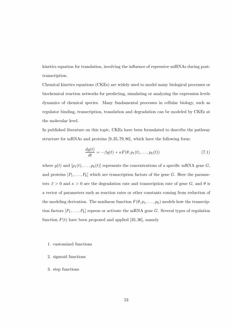
structure for mRNAs and proteins [9, 35,79,80], which have the following form:

dg(t)

dt= −βg(t) + κF (θ, p1(t), . . . , pk(t)) (7.1)

where g(t) and [p1(t), . . . , pk(t)] represents the concentrations of a specific mRNA gene G,

and proteins [P1, . . . , Pk] which are transcription factors of the gene G. Here the parame-

ters β > 0 and κ > 0 are the degradation rate and transcription rate of gene G, and θ is

a vector of parameters such as reaction rates or other constants coming from reduction of

the modeling derivation. The nonlinear function F (θ, p1, . . . , pk) models how the transcrip-

tion factors [P1, . . . , Pk] repress or activate the mRNA gene G. Several types of regulation

function F (t) have been proposed and applied [35,36], namely

1. customized functions

2. sigmoid functions

3. step functions

53

The often used Hill function Hill(p, θ, n) as a function of concentration p, parameters θ

and n is as follows:

Hill(p, θ, n) =pn

θn + pn

It is based on sigmoid functions, but customized functions can also be derived or justified

by applying adequate chemical kinetics principles, such as the law of mass action or the

Michaelis-Menten law. The variables involved in the CKEs can be concentrations or rela-

tive expression levels of molecules such as proteins, mRNAs, miRNAs and so forth. The

parameters of the CKEs, such as degradation rates, transcription rates, translation rates,

equilibrium constants and so forth, are usually unknown and are often difficult to measure

experimentally with enough accuracy.

Mathematical modeling by nonlinear chemical kinetics equations generates complicated

parameter estimation problems from recorded microarray data.

7.2 Chemical Kinetics Equation for Motif A

Select arbitrarily one mRNA gene ”G” and one miRNA gene ”M”. Call ”P” the protein

generated by the gene ”G”. There are essentially two main modalities of interaction within

the triplet of molecules [”G” ,”P”, ”M”], and we now model these (potential) interactions

by chemical kinetics equations linking the expression levels of these 3 molecules.

The regulatory motif A is a small size interaction model describing how the rate of change

for the expression of ”G” (a downstream mRNA) depends on the expression levels of its up-

stream factors, which include the post-transcriptional repressor miRNA ”M”, and two sets

of proteins rep(G) and act(G), namely the transcriptional repressers and transcriptional

activators of ”G”.

54

7.2.1 Post-transcriptional Repressors and Architectural Interaction Mo-

tif A

The regulatory architectural ”motif A” is a small size interaction model describing how the

rate of change for the expression of ”G” (a downstream mRNA) depends on the expres-

sion levels of its upstream factors, which include the post-transcriptional repressor miRNA

”M”, and two sets of proteins rep(G) and act(G), namely the transcriptional repressors

and transcriptional activators of ”G”.

To model the transcription process involving interactions between these transcription fac-

tors (proteins) and their downstream mRNA ”G”. We introduce a nonlinear chemical

kinetics equation (CKE) similar to the equation proposed in [3,9]. but with a complemen-

tary term encoding the repressive influence of miRNA ”M” on its target mRNA ”G”.

Denote by g(t), p(t) and m(t) the expression levels of molecules ”G” ,”P” and ”M” at time

t. We call {R1, R2, . . .} and {A1, A2, . . .} the proteins belonging respectively to rep(G) and

act(G). Denote by ri(t) and aj(t) the respective expression levels of proteins Ri and Aj .

We thus model motif A by the following chemical kinetics equation:

dg(t)

dt= −βg(t)− vg(t)m(t) + κF (t) (7.2)

where β > 0 is the degradation rate of G, v > 0 is the reaction rate between G and M,

κ > 0 is the transcription rate, and F (t) is the fraction of DNA templates committed to

transcription of the mRNA gene G. The fraction F (t) is modeled by setting

RFi(t) =1

(1 + uiri(t))SRiAFj(t) =

1

(1 + wjaj(t))SAj(7.3)

REP (t) =∏

Ri∈ rep(G)

RFi(t) ACT (t) = 1−∏

Aj∈ act(G)

AFj(t) (7.4)

F (t) = REP (t)ACT (t) (7.5)

55

Here SRi > 0, ui > 0 and SAj > 0, wj > 0 are respectively the number of binding sites

and the affinity constant for the transcriptional factors Ri and Aj .

Note that the transcription repressors Ri combine multiplicatively their individual impacts

RFi(t) in F (t); a similar remark applies to the impacts of the transcription activators.

The term κF (t)dt is the concentration of new G molecules synthesized by transcription

during the small time interval [t, t+ dt].

In the same time interval, the repressive interactions of molecules M and G eliminates

vg(t)m(t)dt molecules of G, and natural decay destructs βg(t)dt molecules of G.

The specific form (7.3) of the fraction F (t) of DNA templates committed to the tran-

scription of gene G has been studied in other contexts by [3, 9]. We give below, in the

last paragraph of this chapter, the main arguments and assumptions which justify the

expression of F (t) in our context.

7.3 Chemical Kinetics Equation for Translation Repressors

7.3.1 Interaction Motif B

The regulatory architectural ”motif B” is a small size interaction model describing how

the rate of change for the expression of a downstream protein P depends on the expression

level of its upstream factors, which include the mRNA gene G producing protein P and

the set rep(G) = [M1,M2, . . .] of miRNA repressing the translation of G. The respective

concentrations at time t of protein P , miRNA genes Mi, and mRNA gene G are denoted

by p(t), mi(t), g(t).

56

7.3.2 CKEs to model motif B architectures

We model motif B interaction architectures by the following chemical kinetics equation ,

which modify the CKEs in [3, 7] by complementary terms:

dp

dt= −γp(t) + λg(t)H(t) (7.6)

RPi(t) =1

(1 + uimi(t))SMi(7.7)

H(t) =∏

Miinrep(G)

RPi(t) (7.8)

where γ > 0 and λ > 0 are resp. the degradation rate and the translation rate for protein

P .

The parameters SMi > 0 and ui > 0 are resp. the number of binding sites and the affinity

constant driving the repressive impact of miRNA Mi on the mRNA gene G. The global

repressive impact of all the miRNA molecules Mi on the translation of G is encoded in

H(t), which decreases when the miRNA concentrations mi(t) increases.

The term H(t) is the fraction of G molecules committed to the translation.

7.4 Biochemical Assumptions and CKEs Derivation for Mo-

tifs A and B

In the main CKE of motif A (see (7.2)), the complementary term −vg(t)m(t) encodes the

down-regulation of the target mRNA ”G” by miRNA ”M”, under the following 2 fairly

natural biochemical assumptions

- Assumption 1: Although there maybe many miRNAs that can bind to the target ”G”, this

57

architectural motif tentatively assumes that ”M” is the only miRNA which can strongly

bind at some specific site of gene ”G”, and that this binding then causes the degradation

of the corresponding molecule ”G”.

- Assumption 2: Once a molecule of ”G” and a molecule ”M” actually bind at this specific

site, then this ”G”-molecule degrades in a very short time interval, before binding within

any other ”M” molecule.

Under these assumptions, we have the following reaction:

M +G → O (7.9)

where the molecules ”O” are the degradation outputs and have concentration o(t). The Law

of Mass Action in chemical kinetics states that the rate at which a chemical is generated is

proportional to the product of the concentrations of the reactants with a proportionality

constant v > 0, so that do(t)dt = vg(t)m(t). This explains the corresponding term −vg(t)m(t)

in the CKE (7.2) of motif A providing the expression dg(t)dt .

To derive the form of the functions F (t) and H(t) in the respective CKEs of motif A and

motif B, we will introduce more assumptions beyond the Assumptions 1 and 2.

The main concepts and rigorous derivations needed to support the form we have adopted

for the function F(t) in the CKE for motif A are quite similar to the essential ideas required

to derive the proper form of H(t) in the CKE of motif B.

Hence we will now focus only on the rigorous derivation of the translation CKE for motif

B, which introduces the main ideas and concepts.

Recall first that in [3], the translation process of a gene ”G” generating the protein ”P” is

driven by the following very basic chemical kinetics equation

dp(t)

dt= −γp(t)− λg(t) (7.10)

58

where γ and λ are respectively the degradation rate and the translation rate of protein P .

Here, we need to take into account the complementary repressive influence of the set rep(G)

= [M1,M2, . . .] of miRNA inhibiting the translation of G. We call mj(t) the concentration

of Mj-molecules at time t. We make the following fairly natural assumptions applied for

motif B:

Assumption 3: If a specific molecule of gene ”G” binds with any one of the miRNA repres-

sors Mj listed in rep(G), then this G-molecule will fail to translate.

Assumption 4: As long as a molecule of gene ”G” has bound with none of the miRNA

repressors listed in rep(G), then the translation of this specific G-molecule can initiate

freely.

Assumption 5: Each miRNA repressor Mj of gene G can only bind with gene G at Sj

specific sites; call BINDj this set of Sj specific binding sites . We assume that the sets

BIND1, BIND2, . . . , BINDk of binding sites are pairwise disjoint.

Assumption 6: For any given ”G”-molecule, call Xj the random number of sites in BINDj

which actually bind with ”Mj”-molecules. We assume that the k random variablesX1, ...,Xk

are independent random variables.

The term λg(t) in (7.10) is the concentration of protein ”P”-molecules synthesized per

unit of time when all the molecules of gene G are committed to the translation of ”G”.

However, at any time t, only a fraction of the existing ”G”-molecules t are committed to

the translation of ”G”, due to the inhibiting action of the miRNA repressors of gene G.

So we need compute the fraction of ”G”- molecules which are actually committed to the

translation into protein ”P”-molecules.

Suppose for the moment that k = 1, i.e. that there is only one miRNA gene M = M1 in the

list rep(G) of miRNAs repressing the mRNA gene G. Call S = S1 = cardinal(BIND1)

59

the total number of possible binding sites for the miRNA gene M = M1 on the binding

region of ”G”-molecules.

For 0 ≤ s ≤ S, denote by Gs the set of ”G”-molecules which have exactly s binding sites

actually bound to ”M”-molecules. At time t, call gs(t) the concentration of ”Gs”-molecules,

and m(t) the concentration of miRNA ”M”.

We have the following forward and backward reactions:

G[s] +M ⇀ G[s + 1] (7.11)

G[s+ 1] ⇀ G[s] +M (7.12)

Call mb(t) the concentration of free ”M”-molecules which bind on the ”G[s]”-molecules to

produce ”G[s+1]”-molecules in the forward reaction 7.11. By molecular collision theory

[10], mb is proportional to the product of the total concentration m = m1 of ”M”-molecules

by the concentration of vacant binding sites (S − s) · gs, so that, for some constant cf , we

have

mb(t) = cf (S − s)m(t)gs(t) (7.13)

Call mf (t) the concentration of miRNAs freed by the backward reaction 7.12. Again by

molecular collision theory, mf is proportional to the concentration (s + 1)gs+1 of ”M”-

molecules actually bound to one of the (s+1) occupied binding sites of the ”G”-molecules

belonging to G[s+ 1], so that for some constant cb we have

mf (t) = cb(s+ 1)gs+1(t) (7.14)

At chemical equilibrium, we have naturally mf = mb, and hence

cf (S − s)m(t)gs(t) = cb(s+ 1)gs+1(t)

60

Letting u = cf/cb, we obtain

gs+1(t) = u[(S − s)/(s + 1)]m(t)gs(t)

By an easy recurrence on s, this implies

gs(t) = CsS [um(t)]sg0(t) (7.15)

where the CsS = (S!

s!(S−s)! are the classical binomial coefficients. So the total concentration

g(t) of ”G”-molecules can be expressed by

g(t) =s=S∑

s=0

gs(t) = g0(t)s=S∑

s=0

CsS[um(t)]s = g0(t)[1 + um(t)]S (7.16)

By our assumptions, if at least one of the S = S1 binding sites of a ”G”-molecule is actually

bound to an ”M”-molecule, then this ”G”-molecule will fail to translate, so the fraction

H(t) of ”G”-molecules committed to the translation into protein ”P”-molecules is clearly

given by H(t) = g0(t)g(t) .

In view of the expression (7.16) just obtained we thus have in the case k = 1 of a single

miRNA repressor for gene G.

H(t) =1

[1 + um(t)]S=

1

[1 + um1(t)]S1

(7.17)

So the simple CKE (7.10) for translation must be replaced in our context, and when k = 1,

by

dp

dt= −γp(t) + λg(t)H(t) = −γp(t) + λg(t)

1

[1 + um1(t)]S1

(7.18)

where p(t) is the concentration of protein P , g(t) is the concentration of mRNA gene G

and m1(t) is the concentration of miRNA M = M1.

By recurrence on the number k of miRNA repressors in the list rep(G) = {M1,M2, ...,Mk},

and using the Assumptions 5 and 6 described above, we can extend the argument just

61

given for the case k = 1, and prove that in the generic case where k ≥ 1, then the fraction

H(t) = g0(t)g(t) of ”G”-molecules committed to the translation into protein ”P”-molecules is

given by:

H(t) =

k∏

i=1

1

(1 + uimi(t))Si(7.19)

As we pointed out above, quite similar ideas enable us to derive the form of the function

F (t) and the CKE of motif A.

7.5 Simplified Chemical Kinetics Equations for High Degra-

dation Rate

If there is no protein data available, consider the following equation for translation process

with the assumption that the miRNA repression for the protein levels is ignorable [3]:

dp(t)

dt= −δp(t) + λg(t) (7.20)

In equation 7.20, p(t) is the concentration of a specific protein n at time t, g(t) is the con-

centration of mRNA G, λ is the translation rate of the mRNA G, and δ is the degradation

rate of protein P .

We can see that this equation for the rate of change of protein is different from the equation

we have introduced above. This is a simplified chemical equation proposed by Goutsias

and ignore the influence by the miRNAs.

Equation 7.20 is easy to solve:

p(t) = exp(−δt)p(0) +

ˆ s=t

s=0λ exp(−δ(t− s))g(s) (7.21)

62

We interpolated the data into 19 time points (time unit= 8 hours), the above can be

approximated as:

p(t) = exp(−δt)p(0) +1

2· λ

t−1∑

s=0

[exp(−δ(t− s))g(s) + exp(−δ(t − s− 1))g(s + 1)] (7.22)

Then

p(t) = exp(−δt)p(0)

+1

2λ

t−1∑

s=0

[exp(−δ(t− s))r(s) + exp(−δ(t − s− 1))g(s + 1)]

≤ exp(−δt)p(0) + 1/2λg(t) + λt−1∑

s=0

[exp(−δ(t − s))(g(s))]

= exp(−δt)p(0) + 1/2λg(t) +

λ[exp(−δ)g(t − 1) + exp(−δ · 2)g(t − 2) + ...+ exp(−δt)g(0)]

= exp(−δt)p(0) + λ(0.5g(t) + exp(−δ)g(t − 1) + ...+ exp(−δt)g(0))

If exp(−δ)g(t − 1) < 5% · 0.5g(t), then p(t) ∼ exp(−δt)p(0) + 0.5 · λg(t). For the 11 key

genes we studied in this paper, max(g(t− 1)/g(t)) < 1.7 when t > 0. So

exp(−δ) · g(t)/g(t − 1) < exp(−δ) · 1.7 < 0.05 · 0.5

which gives δ > 4.22, which means the half-life of the protein should be less than ln(2)/4.22·

8 = 1.32 hours (note that the time unit in our equations are 8 hours), Therefore, if δ > 4.22,

p(t) ∼ exp(−δt)p(0) + λ0.5g(t). When

λg(t) >> exp(−deltat)p(0) (7.23)

is satisfied, for t > 0, we have

p(t) ≈ λ · 0.5g(t), t > 1 (7.24)

The above equation means p(t) is approximately proportional to r(t), i.e. p(t) = αg(t),

where α is a constant. This result holds under simplified ODE modeling the translation

63

process, when the associated proteins of the key 11 genes have protein half-life within 1.32

hours and 7.23 is satisfied.

7.6 Formal Invariance of our CKE models by Scale Changes

In most microarray data sets, the ”absolute” expression levels of molecules are not chem-

ically meaningful since they are measured via optical analysis of fluorescence intensities,

but the main biologically meaningful quantities are the relative expression levels between

arbitrary pairs of recorded chemical species. This is one of the reasons why the classical

graphic displays of microarray data by ” heat maps ” actually involve logarithms of the

data.

Since we want to apply our chemical kinetics equations to microarray data sets for which

the most meaningful values are ratios of expression levels data, we will look at how the

chemical kinetics equation changes if we apply generic linear transformations to the ex-

pression data.

Denote by g(t), p(t),m(t) the respective chemical concentrations of mRNA gene G , its

associated protein P , and miRNA gene M targeting G. Assume that g(t), p(t),m(t) are

linked with the concentrations ri(t) and aj(t) of resp. repressive and activating factors

Ri(t) ∈ rep(G) , Aj(t) ∈ act(G), by the following ”motif A” CKE

dg(t)

dt= −βg(t) − vg(t)m(t) + κREP (t)ACT (t) (7.25)

64

where

REP (t) =∏

i

RFi(t) (7.26)

ACT (t) = 1−∏

j

AFj(t) (7.27)

RFi(t) =1

(1 + uiri(t))SRi(7.28)

AFj(t) =1

(1 + wjaj(t))SAj(7.29)

Assume now that the actually recorded expression levels of these molecules, namely

g, p, m, ri, aj are linked to the true concentrations g, p,m, ri, aj by unknown but constant

scale changes, γ, µ, ρi, αj so that we have for all times t the linear relations

g(t) = g(t)/γ, p(t) = p(t)/τ, m(t) = m(t)/µ (7.30)

ri(t) = ri(t)/ρi, aj(t) = aj(t)/αj (7.31)

Define new parameters by the explicit formulas

β = β (7.32)

v = vµ (7.33)

κ = κ/γ (7.34)

ui = ρiui (7.35)

wj = αjwj (7.36)

Then transferring these last two sets of linear relations into the CKE linking the true

concentrations, we obtain the following new CKE where only recorded expression levels

are involved,

dg(t)

dt= −βg(t)− vg(t)m(t) + κREP (t)ACT (t) (7.37)

65

where

REP (t) =∏

i

RF i(t) ACT (t) = 1−∏

j

AF j(t) (7.38)

RF i(t) =1

(1 + uiri(t))SRi= RFi(t) (7.39)

AF j(t) =1

(1 + wj aj(t))SAj] = AFj(t) (7.40)

Note that the algebraic form of this new CKE linking the actual recorded expression

levels of is exactly the same as the algebraic form of the CKE linking the true concen-

trations, but of course with new unknown parameters. The new unknown parameters are

related to the original unknown parameters by scale changes but this has no practical im-

pact, since true concentrations are not accessible through microarray data.

Assume now that each actually recorded gene or protein expression level y(t) is linked by

some linear relation of the type x(t) → y(t) = ax(t) to the true concentration x(t) of the

same gene or protein, where the scale change coefficient can freely depend on the specific

gene or protein considered, but is constant in time.

Our preceding argument shows then that each biochemical hypothesis positing a CKE

model of motif A type between true concentrations is strictly equivalent to assuming that

a similar CKE model of motif A type also holds between recorded expression levels.

Similarly computations easily show that the same global invariance of the models by multi-

ple scale changes is true for CKE models of motif B type. Actually for CKE models of type

B, the global invariance of these CKE models also hold for more general affine relations of

the form. x(t) → y(t) = ax(t) + b between expression levels y(t) and true concentrations

x(t).

One can also prove that the same global invariance by general affine transformations will

hold for a slight algebraic extension of the CKE models of motif A type. After such multi-

ple affine transformations are applied to true concentrations, the new unknown parameters

66

are explicitly linked to the unknown original parameters by non linear relations which are

explicit rational fractions. Of course these relations between parameters have no practical

impact.

The key theoretical result is that we can freely normalize linearly our recorded expression

levels , using different normalizing constants for each recorded gene, before estimating the

parameters of our CKE models of motifA types or of motif B types. Since our Western

Blot protein data are also essentially linearly linked to the corresponding unknown absolute

concentrations, the preceding arguments also applies to cover the case of the actual protein

data we have digitized from Western Blots experimental acquisitions

The preceding global invariance result will also enable us to select an adequate distance

between dynamic profiles of recorded expression levels.

67

Chapter 8

Parameter Estimation for the

CKE models of Motifs A and B

8.1 Parameter Estimation for Nonlinear CKEs

8.1.1 Fitting Chemical Kinetics Dynamic Systems to Data

For actual nonlinear CKE modeling of biochemical processes, estimating the parameters

involved in these CKEs is a major challenge. Model size strongly increases the complexity

of parameter estimation, and can involve very large amounts of computing time in our

context , due to the huge number number of potential genes interaction architectures.

In our context, massive modeling by non linear CKE and estimation of their unknown pa-

rameters is not feasible ”blindly” due to the magnitude of the number of CKEs (more than

30,000 kinetics equations) and the combinatorial complexity for the selection of directly

interacting pairs of genes. Moreover the CKEs we introduce to model the interactions

68

between miRNAs and mRNAs are strongly nonlinear and involve 5 to 10 unknown param-

eters per CKE. Parameter estimation in such systems is of course strongly influenced by

measurement errors in microarray data.

8.1.2 Model Sensitivity to Errors in Experimental Data

Errors in expression levels measurements are inevitable in microarray data, due to the

complexity of cellular environments. These errors in measurements are systematically es-

timated and listed by most technical providers of microarray data.

A natural question is then to evaluate the associated uncertainty on the estimated param-

eter values computed from experimental data, as well as model sensitivity to changes in

parameters. To avoid model instability, regularization techniques are used to control the

impact of the noise corrupting the recorded data [13, 42]. Bayesian methods [41], which

can make good use of estimated standard deviations of recorded expression levels, provide

approximate probability distributions for parameter values. But Bayesian methods such

as Markov Chain Monte Carlo (MCMC) techniques, are still too difficult to implement

and/or computationally too expensive when the problem is high dimensional [43].

8.2 Parameter Estimation by Cost Functions Minimization

A predominant strategy for parameter estimation in systems of CKEs or ODEs is to mini-

mize a cost function evaluating the discrepancy between model predictions and experimen-

tal data.

The concrete goal is to find the parameter values which optimize the quality of fit between

69

simulated time-course for concentrations (or expression levels) and associated recorded ob-

servations.

In published applications, optimization methods usually start from an initial guess which

involves more or less intensive global searches in the parameter space. To get a good initial

guess, generic stochastic minimization methods such as artificial genetic algorithms, sim-

ulated annealing, Markov Chain Monte Carlo (MCMC) have been used as global search

techniques [38, 39], as well as ” pattern search” methods [8, 9] or linear code parameter

search [6].

The genetic algorithm (GA) is a search heuristic that mimics the process of natural evo-

lution. This heuristic is routinely used to generate useful solutions to optimization and

search problems. The basic concept of GAs is designed to simulate processes in natural

system necessary for evolution, specifically those that follow the principles first laid down

by Charles Darwin of survival of the fittest.

Simulated annealing is a generalization of a Monte Carlo method for examining the equa-

tions of state and frozen states of n-body systems [38]. It works by emulating the physical

process whereby a solid is slowly cooled so that when eventually its structure is ”frozen”,

this happens at a minimum energy configuration.

Markov Chain Monte Carlo (MCMC) method is a class of algorithms for sampling from

probability distributions based on constructing a Markov chain that has the desired distri-

bution as its equilibrium distribution. MCMC uses the previous sample values to randomly

generate the next sample value, generating a Markov chain as the transition probabilities

between sample values are only a function of the most recent sample value.

Pattern search (PS) refers to a family of numerical optimization methods that do not re-

quire the gradient of the problem to be optimized and PS can hence be used on functions

that are not continuous or differentiable. They varied one theoretical parameter at a time

70

by steps of the same magnitude, and when no such increase or decrease in any one pa-

rameter further improved the fit to the experimental data, they halved the step size and

repeated the process until the steps were deemed sufficiently small [59]. A linear code is

a subspace of a finite dimensional vector space over a finite field. The linear code param-

eter search algorithm (LCPS) was developed out of the need to survey high dimensional

parameter spaces in which varying one or two parameters at a time, while keeping the

others fixed, is simply not feasible. It has at its core a (not necessarily linear nor binary)

code with efficient covering properties of the high dimensional parameter space [6]. More

specifically, it is essential to find out the minimum covering radius of a code.

Combined with such global search results, local methods such as gradient descent tech-

niques have also been used to minimize these types of cost functions, but mostly for smaller

scale problems involving much smaller sets of CKEs.

8.2.1 An example of parameter estimation techniques for systems of

CKEs

For instance, in paper [10], CKEs with 9 equations were formulated for a chemical system

of reactions. These 9 equations involve 113 parameters. 31 experiments were performed

with variations in the initial concentrations of three molecules and the time intervals, which

provides 9× 31 equations.

So the ratio of the number of data points to the number of parameters is 279/113 ≈ 2.47

which is quite low, and this is certainly an undesirable feature from a purely statistical

point of view.

Then the parameter estimation problem was converted into an optimization problem with

71

loss function

Loss(PAR) =

31∑

j=1

wj ||zj(t)− J(PAR, t)j ||2

Where wj = 1/||zj ||2 is the scalar weight, zj(t) is the measured data for the jth experiment

at time t, and the norm is weighted square norm in L2 space.

The minimization problem was solved by a combined use of global and local optimiza-

tion techniques. Global searches of the admissible space of parameters were performed by

the MATLAB routines ”ga” and ”patternsearch” which implement artificial genetic algo-

rithms and pattern search algorithms to provide suitable candidates as initialization values

for subsequent local searches.

In [10], these local searches were implemented by the MATLAB code ”fmincon”, which

encodes a sequential quadratic programming algorithm. As the name implies, sequential

quadratic programming (SQP) methods are iterative methods solving at each iteration a

quadratic programming problem (QP), which is a linearly constrained optimization prob-

lem with a quadratic objective function [60].

The approach in [10] still required the use of published bounds defining the adequate ranges

for the unknown parameters.

8.2.2 Parameter Estimation Strategy Adopted in Our Study

Stochastic minimization algorithms typically require large amounts of computing time, a

drawback which becomes prohibitive when the number of unknown parameters is high, and

gradient descent methods strongly depend on their initialization points. So generic meth-

ods for cost minimization are generally less efficient than specifically designed strategies

adapted to a specific form of cost function.

72

We have hence developed our own algorithms to estimate the parameters of our CKEs

based models from microarray data and to then compute the quality of fit between mod-

els and data. In our work, this quality of fit, adequately balanced by strongly favoring

parsimoniously parametrized models, becomes an essential clue to decide which potential

interactions we should validate between miRNAs, mRNAs, and the associated proteins.

Reducing the combinatorial complexity by focusing on biologically meaningful architectural

motifs is another essential step we have adopted to increase the ratio of ”number of data

points” over the ”number of unknown parameters”. Thus we have focused on a key genes

known to be involved in ES cells differentiation, such as GCNF, Oct4, Nanog, Sox2, Klf4,

Esrrb, cMyc, Tbx3, Ezh1, Ezh2, Eed, and on pairs of miRNA and mRNA genes which are

listed as potentially interacting in the published tables Targetscan and miRanda.

8.3 Parsimony in Parameters Identification

Our CKEs based models are build and parametrized to enable a robust discrimination

between actual interacting pairs of between miRNA and mRNA genes, and non interacting

pairs of miRNA and mRNA genes.

To increase the robustness of the model, and according to major statistical results due to

Vapnik [82], one should increase the ratio of the the number of data points over the number

of unknown parameters in the model.

Consider the following equation:

dg(t)

dt= κF (t)− vm(t)g(t) − βg(t)

73

Where the fraction function F (t) is:

F (t) =∏

i∈rep(G)

1

(1 + uiri(t))SRi[1−

∏

j∈act(G)

1

(1 + wjaj(t))SAj]

Denote nA to be the number of activators, nR be the number of repressors, then the

number PAR of unknown parameters we need to estimate for each such CKE is PAR =

3+2(nA + nR). Let T be the number of data points available for each one of the recorded

expression levels g(t), m(t), ai(t) and rj(t), t = t1, t2, . . . , tN . Then for each mRNA, these

T data generate T constraints on the unknown parameters of the corresponding CKE.

The Vapnik results show us that good accuracy of parameter estimates require fairly high

values of the ratio of T/PAR. So PAR << T is a necessary constraint. If PAR > T , then

the models are generally overfitted and the parameters are poorly estimated.

Since there are only 38 data points after interpolation for WT and KO, this yields the

following strong constraint on the number of parameters, namely nA + nR ≤ 3.

8.4 Estimation of Parameters by Gradient Descent

Here we take a simple model for example. For a fixed protein P and upstream miRNA M ,

the equation to solve is the following:

dp(t)

dt= λg(t)

1

(1 + um(t))S+ γp(t) (8.1)

Suppose miRNA M is a repressor candidate of protein P , and suppose that γ, u are fixed,

then we want to minimize the following function:

Z(λ, γ, u, S) =∑

t

[p(t)− p(0) +

ˆ t

0(λp(t)− γg(t)

1

(1 + um(t))S)]2 (8.2)

where´ t0 is a notation for mid-point Riemann sum on interval [0, t]. We tested the gradient

descent method to solve the minimization problem. First of all, we want to pick up a ”good”

74

initial value of parameters (γ, λ, u, S), usually by crude search or using the Matlab functions

such as ”ga”. It would be better to find out the range of the parameters before applying

global search. However degradation rate γ and λ is unaccessible for most proteins. And

since there are only a few fraction of all mRNAs that have more than one binding sites for

miRNAs and only .02% mRNAs have as many as 7 binding sites [63], so it is reasonable

for us to restrict 0 ≤ S ≤ 7.

If 1(1+um(t))S

≤ .05, then it means that only 5% of all the mRNAs are committed to translate

the proteins, i.e., over 95% of the mRNAs are bound by the miRNAs. From the findings

in [63] that the miRNA does not act like a genetic switch, and that the miRNAs play a

general role of fine-tuning in gene expression, so we do not expect that there are too many

mRNAs bound by the miRNAs, which would cause an dominated effect to gene expression.

Thus we can restrict u by the following:

max(1

(1 + um(t))S) > 0.05

and solve the upper bound of u, denoted as umax.

With γ > 0, λ > 0, u ∈ [0, umax], S ∈ [1, 7], we applied the Matlab function ”ga”

or ”patternsearch” and get an initial vector of parameters [γ0, λ0, u0, S0]. To implement

gradient descent, we set up the cost function Z(γ, λ, u, S):

Z(γ, λ, u, S) =∑

t

(p(t)− p(0) +

ˆ t

0γp(t)− λ(k)g(t)

1

(1 + um(t))S)2 (8.3)

75

Then we take the partial derivative of the function Z(γ, λ, u, S).

dZ

dγ= 2

∑

t

(p(t)− p(0) +

ˆ t

0[λp(t)− γg(t)

1

(1 + um(t))S])

ˆ t

0p(t)

dZ

dλ= 2

∑

t

(p(t)− p(0) +

ˆ t

0[λp(t)− γg(t)

1

(1 + um(t))S])

ˆ t

0g(t)

1

(1 + um(t))S

dZ

du= 2

∑

t

(p(t)− p(0) +

ˆ t

0[λp(t)− γg(t)

1

(1 + um(t))S])

ˆ t

0[(λSm(t)

1

(1 + um(t))S+1)]

dZ

dS= 2

∑

t

(p(t)− p(0) +

ˆ t

0[λp(t)− γg(t)

1

(1 + um(t))S])(−ˆ t

0λlog(

1

(1 + um(t)))

1

(1 + um(t))S)

Let ∇Z = (dZdβ ,dZdκ ,

dZdu ,

dZdS ), For the nth iteration of gradient descent:

1. take h3 = 1,

(β(n+1), κ(n+1), u(n+1), S(n+1)) = (β(n), κ(n), u(n), S(n))− h3∇Z(n)

2. While Z(n+1) ≥ Z(n), let h3 = h3/2, then renew the value of of Z(n+1) until Z(n+1) <

Z(n), if h3 < TOL, where TOL is a very small number, stop the iteration and keep

(β(n), κ(n), u(n), S(n)) as the solution.

3. If any parameter turns out to be negative, set it to be zero; If S(n+1) > 10, take

S(n+1) = 10.

4. Renew the value of Z(n+1), if Z(n+1) < Z(n), continue, if not, stop with the (β(n), κ(n), u(n), S(n))

as the solution.

8.5 Parameter Estimation Algorithm for the CKEs of Motifs

A and B

There are 2 types of equations we use to model the 2 basic motifs:

dp(t)

dt= −βp(t) + κg(t)H(t)

76

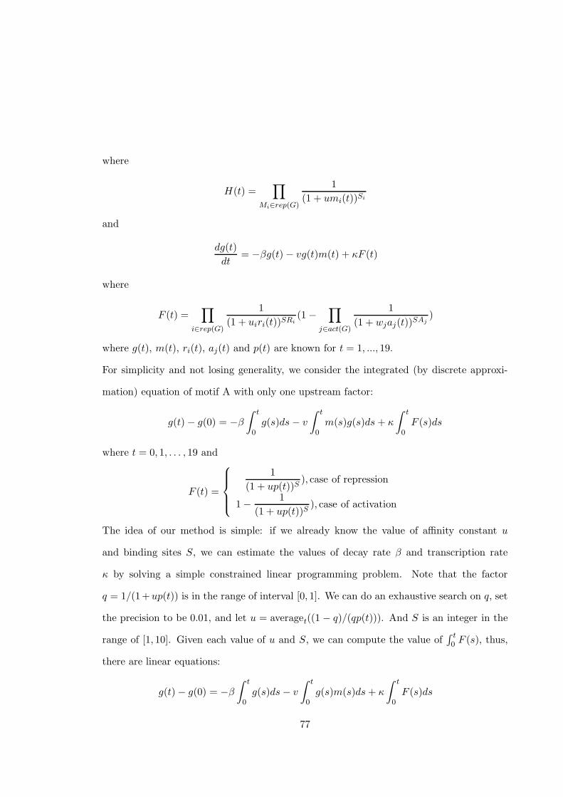
where

H(t) =∏

Mi∈rep(G)

1

(1 + umi(t))Si

and

dg(t)

dt= −βg(t)− vg(t)m(t) + κF (t)

where

F (t) =∏

i∈rep(G)

1

(1 + uiri(t))SRi(1−

∏

j∈act(G)

1

(1 + wjaj(t))SAj)

where g(t), m(t), ri(t), aj(t) and p(t) are known for t = 1, ..., 19.

For simplicity and not losing generality, we consider the integrated (by discrete approxi-

mation) equation of motif A with only one upstream factor:

g(t)− g(0) = −β

ˆ t

0g(s)ds − v

ˆ t

0m(s)g(s)ds + κ

ˆ t

0F (s)ds

where t = 0, 1, . . . , 19 and

F (t) =

1

(1 + up(t))S), case of repression

1− 1

(1 + up(t))S), case of activation

The idea of our method is simple: if we already know the value of affinity constant u

and binding sites S, we can estimate the values of decay rate β and transcription rate

κ by solving a simple constrained linear programming problem. Note that the factor

q = 1/(1+up(t)) is in the range of interval [0, 1]. We can do an exhaustive search on q, set

the precision to be 0.01, and let u = averaget((1 − q)/(qp(t))). And S is an integer in the

range of [1, 10]. Given each value of u and S, we can compute the value of´ t0 F (s), thus,

there are linear equations:

g(t)− g(0) = −β

ˆ t

0g(s)ds − v

ˆ t

0g(s)m(s)ds + κ

ˆ t

0F (s)ds

77

Let

ǫ = maxt

|(t)− g(0) + β

ˆ t

0g(s)ds + v

ˆ t

0g(s)m(s)ds − κ

ˆ t

0F (s)

To minimize ǫ, we can solve the following constrained linear programming problem:

minimize ǫ

subject to −ǫ · 1 < C · x < ǫ · 1

where 1 is a n× 1 vector, n = 19 in this case, x = [β, v, κ], and

C =

(a, b, c

)

where a = [−´ 10 g(s),−

´ 20 g(s), . . . ,−

´ t0 g(s)]

T , b = [−´ 10 g(s)m(s), . . . ,−

´ t0 g(s)m(s)]T ,

c = [−´ 10 F (s), . . . ,−

´ t0 F (s)]T .

Then we will select the best solution of the parameters {u, S, β, v, κ} to minimize ǫ.

Consider a more general case for a fixed mRNA G as the downstream factor, which is

activated by protein P1, repressed by protein P2, and degraded by miRNA M, then we

have the following equation:

dg

dt= −βg(t) − vg(t)m(t) + κF (p1(t), p2(t))

where g(t) is the expression level of downstream mRNA G, p1(t) is the concentration of

P1, p2(t) is the concentration of P2, m(t) is the concentration of M. And

F (p1(t), p2(t)) = (1− 1

(1 + u1p1(t))S1

)1

(1 + u2p2(t))S2

In this example, we need to search the values of u1, S1, u2 and S2, then solve the parameters

β, v and κ by constrained linear programming.

Generally, for these two type of equations, we first do the exhaustive search for the affinity

constants ui and and number of binding sites Si for all i ∈ rep(G)∪act(G), and then apply

78

the constrained linear programming to estimate the other parameters. This algorithm is

relatively fast in computing, on laptop PC it usually takes less than 10 minute to estimate

a 9-parameter model, depending on the precision tolerance the user choose for searching.

The global exhaustive search is for small number of paramters: integer-valued binding

sites Si, which take less than 10 values, and at most 3 affinity constants ui in a small

interval [0,1] and can even take bigger searching steps, such as 0.02 or 0.05 depending on

the number of parameters. It combines a global search method in reasonable precision and

constrained linear programming method, which is easily implemented with high-quality

results. Another advantage of this algorithm is that range of the parameter values are

not required to provide good estimation results, which is very useful for many of these

molecular reaction rates are unaccessible in literature.

8.6 Quality of Fit between Model Predictions and Expres-

sion Levels Data

For a specific motif A or motif B, after algorithmic parametrization of the model in or-

der to achieve the best fit to the two sets of microarray data, we have to evaluate how

well the parametrized model predicts the observed dynamics for the concentration of the

downstream factor.

D(t) = measured expression level of the downstream factor at time t

After actual parametrization of the model, let

D(t) = model-predicted expression of the downstream factor at time t

79

To assess the quality of fit between model prediction of D(t) and recorded microarray data

D(t), it would seem natural to compute the relative error of prediction at time t as follows:

ERR(t) = |D(t)− D(t)|/D(t)

However, the relative error of prediction ERR(t) becomes meaninglessly large whenever

D(t) is close to zero. To avoid these spurious large values, particularly when D(t) visually

agrees quite well with D(t) for all t, we define the smoothed relative error of prediction to

be:

SERR(t) =

ERR(t) if D(t) > 0.15 ·mean(D)

|D(t)− D(t)|/mean(D) if D(t) < 0.15 ·mean(D)

where mean(D) is the average of D(t) over all values of t . Then we define the global error

of prediction err of the model by

err = maxt

(SERR(t))

The error of prediction err quantifies the accuracy level of the parametrized model, and is

percentage valued.

We will say that the model is ”acceptable” or ”validated” if, for both the WT and the KO

microarray data, the ”model error” err is less than 10%, or if err is inferior to the relative

standard deviation of the recorded expression levels.

8.7 Sensitivity of Model Predictions to Small Changes in

Parameters Values

Prediction of expression levels by model of motif type A or B could be possibly very

sensitive to the values of changes for parameters. We here choose only ǫ = 5% as the error

80

0 2 4 60

2000

4000

6000

8000WT: modeling by gradient descent

err=1.750 2 4 6

−2000

0

2000

4000

6000KO: modeling by gradient descent

err=1.16

0 2 4 60

2000

4000

6000

8000WT: modeling by new algo

err=0.050 2 4 6

2000

3000

4000

5000

6000KO: modeling by new algo

err=0.08

Figure 8.1: An example of comparison for estimation results from gradient descent and our

innovative algorithm. blue line=measured expression level; red dash line= model prediction

from the estimated parameters. Top left and right= measured data and modeling prediction

from parameters estimated by gradient descent algorithm for WT and KO data, bottom

left and right=measured data and modeling prediction from parameters estimated by our

innovative algorithm for WT and KO data

tolerances of the parameters, and see numerically how the model predictions vary when

we vary one parameter and fix the others. Denote the parameter we select to change to

be PAR0, and we randomly choose 50 values by uniform distribution, denoted as PARi

for i = 1, . . . , 50, from interval PAR0 · [1 − ǫ, 1 + ǫ] and simulate 50 curves for each value

PARi. Denote the original model error computed from PAR0 as err0, and the maximum

model error out of the 50 simulations as errmax. The results show that the CKEs of motif

type A or B are not much sensitive to parameters. We take a look at an example of motif

A with parameters (β, κ, v, u1, u2, u3, S1, S2, S3) as follows: downstream mRNA=Oct4

miRNA = mmu-mir-186

81

transcription repressor= GCNF

transcription activators= Oct4, Nanog

This example has a very good model prediction with model error err0 = 0.05 and 0.08

respectively for WT and KO. We choose 5% as the error tolerance, and select parameter

β, Then we get errmax = 0.13 for WT simulation, and errmax = 0.15 for KO simulation

(see figure 8.2). Figure 8.3 shows that when κ changes in the error tolerance of 5%,

errmax = 0.08 and 0.17 respectively for WT and KO simulations. Figure 8.4 shows that

when v changes in the error tolerance of 5%, errmax = 0.18 and 0.14 respectively for WT

and KO simulations. Figure 8.5, 8.6 and 8.7 show that when u1oru2oru3 changes in the

error tolerance of 5%, the values of errmax are almost stable respectively for WT and KO

simulations.

For (S1, S2, S3), they all equal to 1, which they are number of binding sites, are integers.

So first we shift up by 1 for each of these three parameters and keep the other two fixed,

and see from Figure 8.8,8.9, 8.10 that errmax for these three cases are no bigger than 0.18,

in which the model fitting is not bad.

Parameter estimation gives us S1 = S2 = S3 = 1 in this example. When we shift down

by 1 for each of these three parameters and keep the other two fixed, then we have three

cases:

• S1 = 0, S2 = S3 = 1, which means protein GCNF is excluded as the repressor for

mRNA Oct4, then errmax = 2.34 for WT. Figure 8.11 shows this prediction fits the

measured data very badly.

• S2 = 0, S1 = S3 = 1, which means protein Oct4 is excluded as the activator for

mRNA Oct4, then errmax = 0.13 for KO. Figure 8.12 shows this prediction fits the

measured data fairly well.

82

• S3 = 0, S2 = S1 = 1, which means protein Nanog is excluded as the activator for

mRNA Oct4, then errmax = 1.32 for KO. Figure 8.13 shows this prediction fits the

measured data very badly.

0 2 4 6−1000

0

1000

2000

3000

4000

5000

6000

7000WT Oct4

err0=0.05 err

max=0.13

0 2 4 62000

2500

3000

3500

4000

4500

5000

5500

6000KO Oct4

err0=0.08 err

max=0.15

Figure 8.2: Display of predictions for mRNA Oct4 of motif A when parameter

β changes for WT and KO. The downstream factor has upstream proteins GCNF,

Oct4, Nanog, and miRNA mmu-mir-186. Blue line = measured expression level, red

dash line=predicted expression level by originally estimated parameters, green dotted

lines=predicted expression levels by modifying the PAR0 to be PARi.

83

0 2 4 60

1000

2000

3000

4000

5000

6000

7000WT Oct4

err0=0.05 err

max=0.06

0 2 4 62000

2500

3000

3500

4000

4500

5000

5500

6000KO Oct4

err0=0.08 err

max=0.17


κ changes for WT and KO. The downstream factor has upstream proteins GCNF,




8.8 Sensitivity of Parameter Estimates to Errors on Expres-

sion Levels

In microarray data, recorded expression levels are corrupted by backgound ”noise” , and

the microarray data sets actually report estimated values of the standard deviation for the

error of measurement on each recorded expression level. We have undertaken the eval-

uation of the corresponding uncertainty on estimated parameter values computed from

experimental data. This is a highly intensive computing task since each one of the more

84

0 2 4 6−1000

0

1000

2000

3000

4000

5000

6000

7000WT Oct4

err0=0.05 err

max=0.19

0 2 4 62000

2500

3000

3500

4000

4500

5000

5500

6000KO Oct4

err0=0.08 err

max=0.14


v changes for WT and KO. The downstream factor has upstream proteins GCNF,




than 10,000 instances of motif A or motif B architectures we had retained for algorithmic

parametrization potentially requires a separate computer analyzis to quantify the impact

of measurement errors on the estimated parameters. This massive computerized validation

is not yet completed, so here we simply present some of the main steps invoved in its

implementation.

A first approach we have tested is to simulate random perturbations of the recorded expres-

sion levels for a specific downstream or upstream factor, where the simulations adds white

noise errors to each relevant recorded expression level value, with the adequate standard

deviation actually attached to each measurement reported in the microarray data set. We

85

0 2 4 60

1000

2000

3000

4000

5000

6000

7000WT Oct4

err0=0.05 err

max=0.06

0 2 4 62500

3000

3500

4000

4500

5000

5500

6000KO Oct4

err0=0.08 err

max=0.08

Figure 8.5: Display of predictions for mRNA Oct4 of motif A when param-

eter u1 changes for WT and KO. The downstream factor has upstream proteins

GCNF, Oct4, Nanog, and miRNA mmu-mir-186. Blue line = measured expression level,

red dash line=predicted expression level by originally estimated parameters, green dotted


then re-estimate the CKE model parameters, but using these artificially perturbed data .

The re-estimation steps are the following.

1. Select a downstream (or upstream) factor FA in a specific CKE model of motif A or

motif B type. Simulate 50 randomly perturbed evolution profiles of the factor FA,

as we did in section 3.4, and keep the expression levels of all other downstream or

upstream factors unchanged.

2. Keep fixed all the values of affinity constants ui, wj and number of binding sites

SRi, SAj asssociated to the various repressors and activators involved in the CKE

86

0 2 4 60

1000

2000

3000

4000

5000

6000

7000WT Oct4

err0=0.05 err

max=0.05

0 2 4 62500

3000

3500

4000

4500

5000

5500

6000KO Oct4

err0=0.08 err

max=0.08






model. These fixed values are pre-estimated from the original recorded expression

levels, as explained above.

3. Then for each one of the 50 simulated perturbed profile of FA, we re-estimate all the

other parameters by our fast constraint linear programming.

4. Call PAR0 the parameters of the CKE model estimated from the original recorded

microarray data. Let PARk be the parameters (of this CKE model) generated by

re-estimation from the kth simulated perturbed dataset.

5. Compute the empirical mean valuesMEANPAR and standard deviations STDPAR

87

0 2 4 60

1000

2000

3000

4000

5000

6000

7000WT Oct4

err0=0.05 err

max=0.05

0 2 4 62500

3000

3500

4000

4500

5000

5500

6000KO Oct4

err0=0.08 err

max=0.08






of the random re-estimated vectosr PAR = [PAR1, . . . , PAR50].

Note that in our approach for parameter estimation, we perform first an exhaustive search

for the affinity constants and number of binding sites, and then implement a constraint lin-

ear programming algorithm to estimate the other parameters. Fixing the values of affinity

constants and of the number of binding sites strongly reduces the computing time of each

parameterre-estimation, but provides nevertheless a good exploration of the robustness to

noise for our constraint linear programming algorithm.

88

0 2 4 6−1000

0

1000

2000

3000

4000

5000

6000

7000WT Oct4

err0=0.05 err

max=0.18

0 2 4 62500

3000

3500

4000

4500

5000

5500

6000KO Oct4

err0=0.08 err

max=0.08


eter S1 changes for WT and KO. The downstream factor has upstream proteins




8.8.0.0.1 Example 1 : Robustness Study for a motif A model. We consider the

following motif A.

G =downstream factor= mRNA gene Oct4

M = miRNA degrader= mmu-mir-186

R1 =transcription repressor= GCNF

A1 = transcription activator= protein Oct4

A2 = transcription activator=protein Nanog

This CKE model involves 9 parameters (β, κ, v, u1, w1, w2, SR1, SA1, SA2) . All affinity

constants (u1, w1, w2) and number of binding sites (SR1, SA1, SA2) are deliberately kept

89

0 2 4 60

1000

2000

3000

4000

5000

6000

7000WT Oct4

err0=0.05 err

max=0.05

0 2 4 62500

3000

3500

4000

4500

5000

5500

6000KO Oct4

err0=0.08 err

max=0.12






fixed.

We choose G as the factor FA to be submitted to 50 random perturbations at each time

point, and we re-estimate 50 vectors of parameter values PARi, i = 1, . . . , 50 for the vector

[β, κ, v].

The initial estimates computed from the original recorded expression levels downstream

are

β0 = 0.091, κ0 = 414, v0 = 0.001

90

0 2 4 60

1000

2000

3000

4000

5000

6000

7000WT Oct4

err0=0.05 err

max=0.05

0 2 4 62500

3000

3500

4000

4500

5000

5500

6000KO Oct4

err0=0.08 err

max=0.18






After 50 simulated perturbations of theG expression levels and corresponding re-estimations

for these 3 parameters, we obtained 50 estimated values for each parameter, namely βi, κi

and vi, for i = 1, . . . , 50. Then we computed the empirical means and standard deviations

for each one of these 3 parameters :

MEANβ = 0.097, STDβ = 0.091

MEANκ = 439, STDκ = 117

MEANv = 0.001 STD(v) = 6× 10−4

91

0 2 4 60

1000

2000

3000

4000

5000

6000

7000WT Oct4

err0=0.05 err

max=2.34

0 2 4 62500

3000

3500

4000

4500

5000

5500

6000KO Oct4

err0=0.08 err

max=0.08






8.8.0.0.2 Example 2 : Robustness study for a motif A model. We consider the

following motif A.

G = downstream factor= mRNA gene Sox2

M = miRNA degrader= mmu-mir-21

A1 = transcription activator= protein Oct4, A2 = transcription activator= protein Nanog

This model involvess 7 parameters (β, κ, v, w1, w2, SA1, SA2).

92

0 2 4 60

1000

2000

3000

4000

5000

6000

7000WT Oct4

err0=0.05 err

max=0.06

0 2 4 62000

2500

3000

3500

4000

4500

5000

5500

6000KO Oct4

err0=0.08 err

max=0.13






All affinity constants (w1, w2) and number of binding sites (SA1, SA2) are fixed. We choose

G as the factor FA to be perturbated and we implemented 50 random perturbations of the

recorded expression levels of G. We then generated 50 re-estimated vectors of parameters

values PARi, i = 1, . . . , 50 for β, κ and v The initial estimation computed from the original

recorded expression levels downstream are

β0 = 0.08, κ0 = 380.00, v0 = 6× 10−6

93

0 2 4 6−1000

0

1000

2000

3000

4000

5000

6000

7000WT Oct4

err0=0.05 err

max=0.22

0 2 4 6−2000

−1000

0

1000

2000

3000

4000

5000

6000KO Oct4

err0=0.08 err

max=1.32






The empirical means and standard deviations computed from 50 re-estimated values of

these 3 parameters were the following.

MEANβ = 0.05, STDβ = 0.04

MEANκ = 263 STDκ = 158

MEANv = 7× 10−6 STD(v) = 1.5× 10−6

8.8.0.0.3 Example 3: Robustness study for a motif B model. We consider the

following motif B.

94

P = downstream factor= protein Oct4

M1 = miRNA repressor= mmu-miR-542-3p

M2 = miRNA repressor=mmu-miR-484

M3 = miRNA repressor= mmu-miR-138

This model involves 8 parameters (β, κ, u1, u2, u3, S1, S2, S3). All affinity constants (u1, u2, u3)

and number of binding sites (S1, S2, S3) are fixed. We simulated 50 randomly perturbed

expression levels for the downstream factor P , and re-estimated 50 vector values PARi,

i = 1, . . . , 50 for the parameters β, κ. The estimates computed from the original recorded

expression levelswere the following:

β0 = 0.27, κ0 = 9× 10−5

After 50 random perturbations and simulations and re-estimations for these 2 parameters,

we computed the empirical means and standard deviations for the parameter estimates .

MEANβ = 0.27, STDβ = 0.03

MEANκ = 9× 10−5 STDκ = 1.3× 10−5

8.8.0.0.4 Example 4 : Robustness study for a motif B model. We consider the

following motif B, quite similar in structure to the preceding one.

P = downstream factor= protein Oct4

M1 = miRNA repressor= mmu-miR-542-3p

M2 = miRNA repressor=mmu-miR-369-5p

M3 = miRNA repressor= mmu-miR-138

This model involves 8 parameters (β, κ, u1, u2, u3, S1, S2, S3). All affinity constants (u1, u2, u3)

and number of binding sites (S1, S2, S3) are fixed. The initial parameter values (computed

95

from original data ) of β, κ were

β0 = 0.2656, κ0 = 8.6903 × 10−5

After 50 simulated perturbations of the downstream factor P , and corresponding re-

estimations of the 2 parameters β, κ , we obtained the empirical means and standard

deviations of their estimators.

MEANβ = 0.27, STDβ = 0.03

MEANκ9× 10−5 STDκ = 1.3 × 10−5

8.8.0.0.5 Robustness Evaluations In the above 4 examples, the mean values of the

estimated parameters are reasonably close to the initial ones computed from the original

data.

The standard deviations are relatively large for the first two examples of motif A, and fairly

small for the last two examples of motif B. To explain this, we point out that the standard

deviations of measurements errors are of the order of 10% to 20% of the recorded expression

levels for the genes G in the two motif A models, while for the protein P data involved in

the two examples of model B, we have deliberately selected an optimistic relative value of

5% for the unknown size of measurements errors on protein data.

These examples show that estimated parameters can fluctuate to quite an extent due to the

errors of measurements affecting recorded expression levels. For each motif A or motif B

architecture we have parameterized, we intend to perform this robustness study to confirm

the direct evaluation of the quality of fit. However this second level validation program is

quite costly to complete, and is for the moment still a work in progress, due to the very

large number of architectures we have parametrized.

96

Chapter 9

Model Validated Interactions

between MicroRNAs and mRNA

genes

9.1 Modeling for Basic Motifs of Type A

There are 3 groups of mRNAs we want to study as downstream factors of motif A.

1. (Oct4, Nanog), each of which has transcription repressor GCNF as figure 1. The

potential transcription activators of these two mRNAs are proteins (Oct4, Nanog,

Sox2) [5].

2. Self-renewal regulators (Sox2, Klf4, cMyc, Tbx3, Esrrb). According to figure 1, we

use (Oct4, Nanog) as the transcription activators.

3. Differential inhibitors (Ezh1, Ezh2, Eed). According to figure 1, we use (oct4, Nanog)

97

as the transcription repressors.

For each downstream factor, the potential upstream miRNA degrader could be selected

from the predictions of targetscan and miRanda. Once we fix the downstream gene and

its transcriptional factors and select an miRNA that may target the mRNA from the list

of predictions, we can validate whether this hypothesis is plausible by modeling motif A.

Knowing that GCNF is the key repressor for Oct4 and Nanog, for each miRNA pre-

dicted from miRanda and targetscan, we tried the combinations (GCNF, Oct4), (GCNF,

Nanog), (GCNF, Sox2), (GCNF, Oct4, Nanog), (GCNF, Oct4, Sox2), (GCNF, Nanog,

Sox2), (GCNF, Oct4, Nanog, Sox2) as the upstream TFs for Oct4 and Nanog.

The solution and model quality shows that (GCNF, Oct4, Nanog) is the best combina-

tion for both downstream factors Oct4 and Nanog. Together with (GCNF, Oct4, Nanog),

mmu-miR-186, 466, 103 and 107 are the miRNAs such that modeling for mRNA Oct4 are

plausible. And we present the best model for mRNA Nanog, in which the corresponding

miRNA is mmu-miR-139.

We can see in Table 9.1 that most of the validated miRNAs of motif A are in class 2

(transient). The only exception is that all the 12 validated miRNAs for target Ezh2 are in

class 3. There is no validated pair for mRNA Nanog or Esrrb, i.e. no miRNA that directly

degrades mRNA genes Nanog or Esrrb can be validated by modeling the potential pairs

predicted by miRanda or TargetScan. However, our datasets of recorded microarray data

contains only 266 known miRNAs, so we did not have the possibility to include in our

modeling a small group of miRNAs predicted by miRanda or TargetScan but for which we

have no recorded microarray data. Therefore it is possible that more miRNA-mRNA pairs

could be validated by motif A models if the available microarray data had included all the

identified miRNAs available.

98

Table 9.3 presents all validated miRNA-mRNA pairs of motif A for the 11 mRNAs. We

have evaluated 364 models of motif A and found that 88 out of these 364 models of motif

A are validated with model error less than 10%. So there are around 24% motifs of type

A that are validated by modeling.

Table 9.1: Motif A: Number of Validated miRNA-mRNA Pairs

mRNA miRNAs validated validated validated validated

gene G targeting G miRNAs miRNAs miRNAs miRNAs

in class 1 in class 3 in class 2

Oct4 19 6 1 0 5

Nanog 2 0 0 0 0

Sox 2 29 9 4 0 5

Klf 4 44 2 0 0 2

Esrrb 10 0 0 0 0

cMyc 12 12 0 0 12

Tbx 3 18 18 5 0 13

Ezh 1 51 20 6 0 14

Ezh 2 29 12 0 12 0

Eed 25 7 1 1 5

9.2 Modeling of Basic Motif of Type B

We have determined a list of 5337 models of motif B to be validated for the 4 proteins

(Oct4, Nanog, Sox2, GCNF). The computation result shows that there are 51 combinations

99

0 2 4 60

100


0 2 4 60

100


0 2 4 6

2000

4000

6000

WT Oct4

err=0.05 std=0.070 2 4 6

2000

4000

6000

err=0.08 std=0.34

KO Oct40 2 4 6

0

2

4WT transcription factors

0 2 4 60

1

2KO transcription factors

Figure 9.1: Display of a validated motif of type A for Oct4. The top left and

right are profiles of miRNA 186 for WT and KO over day 0-6 respectively. The middle

left and right are profiles of transcription factors of Oct4 for WT and KO over day 0-6

respectively. Blue solid line represents the expression evolution of protein Oct4, green dash

line represents the expression evolution of protein Nanog, red dotted-solid line represents

the expression of protein GCNF. The bottom left and right are profiles of mRNA oct4

for WT and KO respectively. The blue line is the measured expression; the red dash

line is the approximated expression predicted by the model with upstream TF GCNF

as repressor, (Oct4, Nanog) as activators, and miRNA mmu-miR-186 degrading mRNA

Oct4. err represents the model error, std represents the relative standard deviation of the

measurement.

100

0 2 4 60

5


0 2 4 60

5


0 2 4 6

2000

4000

WT Nanog

err=0.14 std=0.050 2 4 6

2000

4000

err=0.05 std=0.20

KO Nanog0 2 4 6

0

2


0 2 4 60

1


Figure 9.2: Display of a motif of type A for nanog. The top left and right are profiles

of miRNA 139 for WT and KO over day 0-6 respectively. The middle left and right are

profiles of transcription factors of Nanog for WT and KO over day 0-6 respectively. Blue

solid line represents the expression evolution of protein Oct4, green dash line represents

the expression evolution of protein Nanog, red dotted-solid line represents the expression

of protein GCNF. The bottom left and right are profiles of mRNA Nanog for WT and KO

respectively. The blue line is the measured expression; the red dash line is the approximated

expression predicted by the model with upstream TF GCNF as repressor, (Oct4, Nanog) as

activators, and miRNA mmu-miR-139 degrading mRNA Nanog. err represents the model

error, std represents the relative standard deviation of the measurement.

101

0 2 4 60

1

2x 10

4 WT mmu−miR−21

0 2 4 62000

4000


0 2 4 6

2000

4000

6000

WT Sox 2

err=0.10 std=0.490 2 4 6

2000

4000

6000

err=0.05 std=0.08

KO Sox 20 2 4 6

0

2


0 2 4 60

1


Figure 9.3: Display of a validated motif of type A for Sox2.The top left and right are

profiles of miRNA 21 for WT and KO over day 0-6 respectively. The middle left and right

are profiles of transcription factors of Sox2 for WT and KO over day 0-6 respectively. Blue

solid line represents the expression evolution of protein Oct4, green dash line represents the

expression evolution of protein Nanog. The bottom left and right are profiles of mRNA

Sox2 for WT and KO respectively. The blue line is the measured expression; the red

dash line is the approximated expression predicted by the model with upstream TF (Oct4,

Nanog) as activators, and miRNA mmu-miR-21 degrading mRNA Sox2. err represents the

model error, std represents the relative standard deviation of the measurement.

102

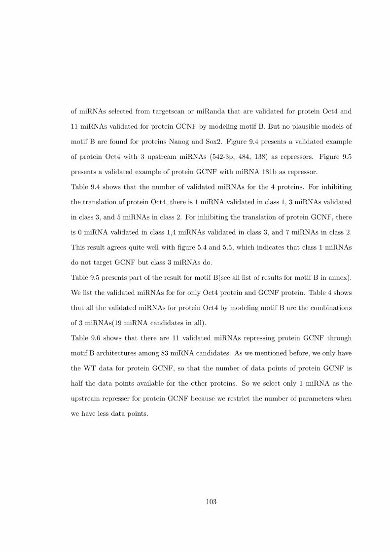
of miRNAs selected from targetscan or miRanda that are validated for protein Oct4 and

11 miRNAs validated for protein GCNF by modeling motif B. But no plausible models of

motif B are found for proteins Nanog and Sox2. Figure 9.4 presents a validated example

of protein Oct4 with 3 upstream miRNAs (542-3p, 484, 138) as repressors. Figure 9.5

presents a validated example of protein GCNF with miRNA 181b as repressor.

Table 9.4 shows that the number of validated miRNAs for the 4 proteins. For inhibiting

the translation of protein Oct4, there is 1 miRNA validated in class 1, 3 miRNAs validated

in class 3, and 5 miRNAs in class 2. For inhibiting the translation of protein GCNF, there

is 0 miRNA validated in class 1,4 miRNAs validated in class 3, and 7 miRNAs in class 2.

This result agrees quite well with figure 5.4 and 5.5, which indicates that class 1 miRNAs

do not target GCNF but class 3 miRNAs do.

Table 9.5 presents part of the result for motif B(see all list of results for motif B in annex).

We list the validated miRNAs for for only Oct4 protein and GCNF protein. Table 4 shows

that all the validated miRNAs for protein Oct4 by modeling motif B are the combinations

of 3 miRNAs(19 miRNA candidates in all).

Table 9.6 shows that there are 11 validated miRNAs repressing protein GCNF through

motif B architectures among 83 miRNA candidates. As we mentioned before, we only have

the WT data for protein GCNF, so that the number of data points of protein GCNF is

half the data points available for the other proteins. So we select only 1 miRNA as the

upstream represser for protein GCNF because we restrict the number of parameters when

we have less data points.

103

0 2 4 60

100

200

300

400

500

600WT mmu−miR−542−3p mmu−miR−484 mmu−miR−138

0 2 4 60

100

200

300

400

500KO mmu−miR−542−3p mmu−miR−484 mmu−miR−138

0 2 4 60

0.5

1

1.5

WT Oct4

accuracy=0.140 2 4 6

0

0.5

1

1.5

accuracy=0.08

KO Oct4

Figure 9.4: Display of a validated motif of type B for Oct4.Protein Oct4 and its

upstream miRNAs profile for WT and GCNF-KO respectively. The upper left is profile of

WT upstream miRNAs. The upper right is profile of KO upstream miRNAs. Blue line is

542-3p expression, green line is 484 expression, red line is 138 expression. In lower graphs,

blue line is the measured expression; the red dash line is the approximated expression

predicted by the model with upstream the The model error of the WT model and of the

KO model are presented below the figures respectively

104

0 1 2 3 4 5 60

2000

4000

6000

8000WT mmu−miR−181b

0 1 2 3 4 5 60

0.5

1

1.5

WT GCNF

accuracy=0.08

Figure 9.5: Display of a validated motif of type B for GCNF.Protein GCNF and

its upstream miRNAs profile in WT. The upper graph is profile of WT upstream miRNA.

Blue line is the measured expression; the red dash line is the approximated expression

predicted by the model with upstream the The model error of the WT model is presented

below the figures

105

9.3 Examples of Invalidated Models of type B for Proteins

Nanog and Sox2

Figure 9.6 presents a model of motif B for protein Nanog. We take 2 miRNAs candidates

repressing protein Nanog [1], no such combination succeeds to provide a plausible model.

This could be due to the lack of enough miRNA candidates in the list that are predicted

to target Nanog by miRanda or TargetScan.

For Sox2, there is no validated model of motif B either. All modeling results for protein

Sox2 show that the translation rate γ is almost zero. So no matter what upstream miRNAs

we select, the modeling prediction for Sox2 are the same as figure 9.7. We can see that the

degradation rate of Sox2 protein in WT cells looks much more greater than in KO cells.

But our modeling made the assumption that the degradation rates in both WT and KO

are the same.

Note that the half-life of a protein like Sox2 may quite possibly change in different cell

cultures; for instance, protein Oct4 has a half-life of 90 minutes in undifferentiated P19

cells [17] and of 6 to 8 hours in NIH3T3 cells transfected with wild type Oct4 [18].

If we now generate parametrized models of the same motif B architecture, but whith the

new assumption that the half-life of protein Sox2 is different for WT cells and for KO

cells, then we obtain much better model predictions displayed in figure 9.8. The estimated

half-life of protein Sox2 is then 20.5 hours for WT cells , and 64.5 hours for KO cells.

Although the half-life of protein Sox2 may be very different in WT and KO, which would

indeed explain the implausible initial modeling results for Sox2, we still need more explicit

biological explanation about the large difference of half-life values.

106

0 2 4 650

100

150


0 2 4 60

20

40

60


0 2 4 60

0.5

1

1.5

2

WT Nanog


0

0.5

1

1.5

2

accuracy=0.18

KO Nanog

Figure 9.6: Display of an invalidated motif of type B for Nanog.Protein Nanog

and its upstream miRNAs profile for WT and GCNF-KO respectively. The upper left is

profile of WT upstream miRNAs mmu-mir-470. The upper right is profile of KO upstream

miRNAs mmu-mir-470. In lower graphs, blue line is the measured expression; the red dash

line is the approximated expression predicted by the model with upstream the The model

error of the WT model and of the KO model are presented below the figures respectively.

9.4 Modeling Hox Cluster

Hox cluster in figure 3 play a very important role in differentiation of ES cells. When Hox

cluster are not repressed by (Ezh1, Ezh2, Eed), they activates the ES differentiation; when

Hox cluster are repressed by (Ezh1, Ezh2, Eed), then ES differentiation are also repressed.

107

0 2 4 62000

4000

6000

8000

10000

12000

14000

16000WT mmu−miR−134 mmu−miR−21

0 2 4 60

1000

2000

3000

4000

5000

6000KO mmu−miR−134 mmu−miR−21

0 2 4 60

0.2

0.4

0.6

0.8

WT Sox 2


0

0.2

0.4

0.6

0.8

accuracy=0.61

KO Sox 2

Figure 9.7: Display of an invalidated motif of type B for Sox2.Protein Sox2 and

upstream miRNAs mmu-mir-134 and 21. Upper left: WT profiles of upstream miRNAs.

Upper right: KO profiles of upstream miRNAs. In lower graphs: blue line = measured

expression levels, red dash line = predicted expression levels. Model errors of prediction

are too large for validation

It is natural to think of modeling Hox cluster by chemical kinetics equation of motif type

A, in which case (Ezh1, Ezh2, Eed) are transcription repressers. Although the protein

expression levels of (Ezh1, Ezh2, Eed) are not available because of technology limitations,

it is possible that combinations of the three proteins (Oct4, Nanog, Sox2) are transcription

108

0 1 2 3 4 5 6−0.1

0

0.1

0.2

0.3

0.4WT Sox2

d=2.72e−001 err=0.22

0 1 2 3 4 5 6−0.5

0

0.5

1

d=8.62e−002 err=0.17

KO Sox2

Figure 9.8: Display of a validated simplified model for Sox2.Protein Sox2 profile for

WT and GCNF-KO respectively. Blue line is the measured expression; the red dash line is

the approximated expression predicted by the model with upstream the The model error

of the WT model and of the KO model are presented below the figures respectively

109

activators/repressers for the Hox cluster for (Oct4, Nanog, Sox2) regulate a relatively large

proportion of genes(Young Lab). It is possible that none of the combinations of the three

proteins (Oct4, Nanog, Sox2) are the transcription factors for a fixed mRNA GH from Hox

cluster, which means that both the proteins and miRNA upstream factors are not identified

for a downstream factor mRNA GH of motif A. Since the miRNA is not considered to

have big influences on the mRNA expression [1], we can first simplify motif of type A

by considering only the interaction of transcription factors and their downstream mRNA.

The following is the chemical kinetics equations involving only interaction of transcription

factors and the downstream mRNA [3]:

dg(t)

dt= βg(t) + κF (t) (9.1)

Where

lF (t) = REP (t)ACT (t)

RFi(t) =1

(1 + uiri(t))SRi, AFj(t) =

1

(1 + wjaj(t))SAj

REP (t) =∏

Riin rep(G)

RFi(t), ACT (t) = 1− S∏

Aj in act(G)

AFj(t)

For a specific mRNA G in Hox cluster, the upstream transcription factors could be 7

possible combinations of (Oct4, Nanog, Sox2): (Oct4), (Nanog), (Sox2), (Oct4, Nanog),

(Oct4, Sox2), (Oct4, Nanog, Sox2). Given 41 mRNAs of Hox cluster, we will have 7× 41

models when transcription factors are activators, 7× 41 models when transcription factors

are repressors. We consider the case that two or three transcription factors, a combination

we listed above, are either all repressors or all activators for the downstream factor. Because

the time course expression levels of these three proteins, by looking at the evolution curves

in WT data( Figure 3.16), are strongly positively correlated. Therefore this defines 574

110

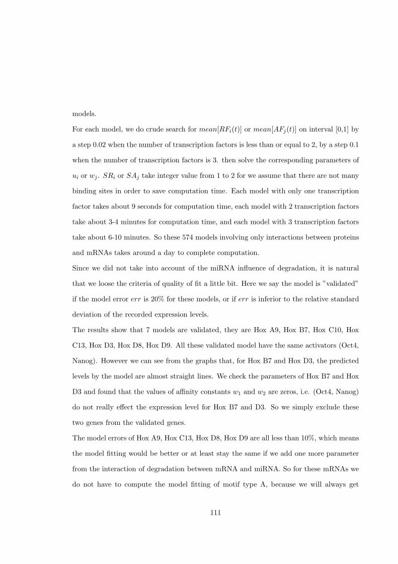
models.

For each model, we do crude search for mean[RFi(t)] or mean[AFj(t)] on interval [0,1] by

a step 0.02 when the number of transcription factors is less than or equal to 2, by a step 0.1

when the number of transcription factors is 3. then solve the corresponding parameters of

ui or wj . SRi or SAj take integer value from 1 to 2 for we assume that there are not many

binding sites in order to save computation time. Each model with only one transcription

factor takes about 9 seconds for computation time, each model with 2 transcription factors

take about 3-4 minutes for computation time, and each model with 3 transcription factors

take about 6-10 minutes. So these 574 models involving only interactions between proteins

and mRNAs takes around a day to complete computation.

Since we did not take into account of the miRNA influence of degradation, it is natural

that we loose the criteria of quality of fit a little bit. Here we say the model is ”validated”

if the model error err is 20% for these models, or if err is inferior to the relative standard

deviation of the recorded expression levels.

The results show that 7 models are validated, they are Hox A9, Hox B7, Hox C10, Hox

C13, Hox D3, Hox D8, Hox D9. All these validated model have the same activators (Oct4,

Nanog). However we can see from the graphs that, for Hox B7 and Hox D3, the predicted

levels by the model are almost straight lines. We check the parameters of Hox B7 and Hox

D3 and found that the values of affinity constants w1 and w2 are zeros, i.e. (Oct4, Nanog)

do not really effect the expression level for Hox B7 and D3. So we simply exclude these

two genes from the validated genes.

The model errors of Hox A9, Hox C13, Hox D8, Hox D9 are all less than 10%, which means

the model fitting would be better or at least stay the same if we add one more parameter

from the interaction of degradation between mRNA and miRNA. So for these mRNAs we

do not have to compute the model fitting of motif type A, because we will always get

111

validated models.

Then we only have to look at Hox C10, which has 4 predicted miRNAs from the list of

targetscan or miRanda. The modeling results show that none of the four miRNAs, which

are (mmu-mir-33, mmu-mir-155, mmu-mir-143, mmu-mir-345), can be validated very well

with the transcriptional factors (Oct4, Nanog) (See figure 9.16 9.17 9.18 9.19)

112

0 2 4 6−1

0

1

2


0 2 4 60.5

1

1.5


0 2 4 6

60

65

70

75

80

85

WT Hox B7

err=0.16 std=0.080 2 4 6

60

65

70

75

80

85

err=0.15 std=0.07

KO Hox B7

Figure 9.9: Modeling fitting result of Hox B7. Top left and right are expression levels

of Oct4 and Nanog proteins for WT and KO context respectively, where blue line is Oct4

protein, green line is Nanog protein. Bottom left and right are expression levels of mRNA

Hox B7 for WT and KO respectively. Blue line is the observed expression level of Hox

B7, red dash line is the model prediction of Hox B7. ”err”=model error, ”std”=standard

deviation of measurement.

113

0 2 4 6−1

0

1

2


0 2 4 60.5

1

1.5


0 2 4 6

200

400

600

800

1000

1200

WT Hox A9

err=0.11 std=0.070 2 4 6

200

400

600

800

1000

1200

err=0.11 std=0.17

KO Hox A9

Figure 9.10: Modeling fitting result of Hox A9. Top left and right are expression levels



Hox A9 for WT and KO respectively. Blue line is the observed expression level of Hox

A9, red dash line is the model prediction of Hox A9. ”err”=model error, ”std”=standard


114

0 2 4 6−1

0

1

2


0 2 4 60.5

1

1.5


0 2 4 6120

140

160

180

200WT Hox C10

err=0.15 std=0.060 2 4 6

120

140

160

180

200

err=0.15 std=0.10

KO Hox C10

Figure 9.11: Modeling fitting result of Hox C10. Top left and right are expression

levels of Oct4 and Nanog proteins for WT and KO context respectively, where blue line

is Oct4 protein, green line is Nanog protein. Bottom left and right are expression levels

of mRNA Hox C10 for WT and KO respectively. Blue line is the observed expression

level of Hox C10, red dash line is the model prediction of Hox C10. ”err”=model error,

”std”=standard deviation of measurement.

115

0 2 4 6−1

0

1

2


0 2 4 60.5

1

1.5


0 2 4 6

70

80

90

100

WT Hox C13

err=0.08 std=0.050 2 4 6

70

80

90

100

err=0.08 std=0.12

KO Hox C13

Figure 9.12: Modeling fitting result of Hox C13. Top left and right are expression

levels of Oct4 and Nanog proteins for WT and KO context respectively, where blue line

is Oct4 protein, green line is Nanog protein. Bottom left and right are expression levels

of mRNA Hox C13 for WT and KO respectively. Blue line is the observed expression

level of Hox C13, red dash line is the model prediction of Hox C13. ”err”=model error,

”std”=standard deviation of measurement.

116

0 2 4 6−1

0

1

2


0 2 4 60.5

1

1.5


0 2 4 6

400

450

500

WT Hox D3

err=0.11 std=0.090 2 4 6

400

450

500

err=0.13 std=0.08

KO Hox D3

Figure 9.13: Modeling fitting result of Hox D3. Top left and right are expression levels



Hox D3 for WT and KO respectively. Blue line is the observed expression level of Hox

D3, red dash line is the model prediction of Hox D3. ”err”=model error, ”std”=standard


117

0 2 4 6−1

0

1

2


0 2 4 60.5

1

1.5


0 2 4 6

100

200

300

400

500

WT Hox D8

err=0.08 std=0.050 2 4 6

100

200

300

400

500

err=0.06 std=0.10

KO Hox D8







118

0 2 4 6−1

0

1

2


0 2 4 60.5

1

1.5


0 2 4 6100

150

200

250

300

350

WT Hox D9

err=0.08 std=0.030 2 4 6

100

150

200

250

300

350

err=0.04 std=0.08

KO Hox D9







119

0 2 4 61

2

3WT mmu−miR−33

0 2 4 60

2

4KO mmu−miR−33

0 2 4 60

2


0 2 4 60

1


0 2 4 6

150

200WT Hox C10

err=0.14 std=0.080 2 4 6

150

200

err=0.14 std=0.08

KO Hox C10

Figure 9.16: Modeling fitting result of Hox C10 of motif type A. Top left and right

are expression levels of miRNA mmu-mir-33 for WT and KO context respectively. Middle

left and right are expression levels of Oct4 and Nanog proteins for WT and KO context

respectively, where blue line is Oct4 protein, green line is Nanog protein. Bottom left and

right are expression levels of mRNA Hox C10 for WT and KO respectively. Blue line is the

observed expression level of Hox C10, red dash line is the model prediction of Hox C10.

”err”=model error, ”std”=standard deviation of measurement.

120

0 2 4 60

500


0 2 4 60

1000


0 2 4 60

2


0 2 4 60

1


0 2 4 6

150

200WT Hox C10

err=0.15 std=0.080 2 4 6

150

200

err=0.15 std=0.08

KO Hox C10








121

0 2 4 60

200


0 2 4 60

200


0 2 4 60

2


0 2 4 60

1


0 2 4 6

150

200WT Hox C10

err=0.15 std=0.080 2 4 6

150

200

err=0.15 std=0.08

KO Hox C10








122

0 2 4 6100

200


0 2 4 60

100


0 2 4 60

2


0 2 4 60

1


0 2 4 6

150

200WT Hox C10

err=0.15 std=0.080 2 4 6

150

200

err=0.15 std=0.08

KO Hox C10








123

Table 9.2: Motif A: Validated miRNA-mRNA Pairs

class miRNA mRNA class miRNA mRNA

2 mmu-miR-186 Oct4 2 mmu-miR-186 Oct4



1 mmu-miR-21 Sox 2 2 mmu-miR-26a Tbx 3

1 mmu-miR-290 Sox 2 1 mmu-miR-15b Ezh 1

1 mmu-miR-292-5p Sox 2 1 mmu-miR-15a Ezh 1

2 mmu-miR-129-3p Sox 2 1 mmu-miR-16 Ezh 1

2 mmu-miR-431 Sox 2 2 mmu-miR-195 Ezh 1



1 mmu-miR-19b Sox 2 2 mmu-miR-301 Ezh 1

2 mmu-miR-19a Sox 2 2 mmu-miR-329 Ezh 1

2 mmu-miR-19a Klf 4 1 mmu-miR-291a-3p Ezh 1

2 mmu-miR-29b Klf 4 2 mmu-miR-323 Ezh 1

2 mmu-let-7i cMyc 2 mmu-miR-22 Ezh 1

2 mmu-let-7c cMyc 2 mmu-miR-302c Ezh 1

2 mmu-let-7b cMyc 2 mmu-miR-183 Ezh 1

2 mmu-let-7f cMyc 2 mmu-miR-145 Ezh 1

2 mmu-miR-212 cMyc 1 mmu-miR-15a Ezh 1

2 mmu-miR-98 cMyc 1 mmu-miR-16 Ezh 1



124

Table 9.3: Motif A: Validated miRNA-mRNA Pairs (continued)


2 mmu-miR-135b cMyc 2 mmu-miR-345 Ezh 1

2 mmu-miR-135a cMyc 2 mmu-let-7f Ezh 2

2 mmu-miR-340 cMyc 2 mmu-let-7a Ezh 2

2 mmu-miR-106b Tbx 3 2 mmu-let-7b Ezh 2

1 mmu-miR-17-3p Tbx 3 2 mmu-let-7c Ezh 2

1 mmu-miR-17-5p Tbx 3 2 mmu-let-7d Ezh 2

2 mmu-miR-106a Tbx 3 2 mmu-let-7g Ezh 2

1 mmu-miR-93 Tbx 3 2 mmu-let-7i Ezh 2

1 mmu-miR-20a Tbx 3 2 mmu-let-7e Ezh 2

2 mmu-miR-20b Tbx 3 2 mmu-miR-98 Ezh 2

2 mmu-miR-126-5p Tbx 3 2 mmu-miR-26a Ezh 2

2 mmu-miR-142-3p Tbx 3 2 mmu-miR-26b Ezh 2

1 mmu-miR-466 Tbx 3 2 mmu-miR-98 Ezh 2

2 mmu-miR-338 Tbx 3 2 mmu-miR-1 Eed


2 mmu-miR-26b Tbx 3 2 mmu-miR-34b Eed

2 mmu-miR-146 Tbx 3 2 mmu-miR-101a Eed

2 mmu-miR-469 Tbx 3 2 mmu-miR-30a-3p Eed

2 mmu-miR-142-5p Tbx 3 2 mmu-miR-301 Eed


125

Table 9.4: Motif B: Number of Validated miRNAs

protein miRNAs validated validated validated validated

G targeting G miRNAs miRNAs miRNAs miRNAs

in class 1 in class 2 in class 2

Oct4 19 9 1 3 5

GCNF 83 11 0 4 7

Nanog 2 0 0 0 0

Sox2 29 0 0 0 0

126

Table 9.5: Motif B: Validated MiRNAs Repressing Oct4

class miRNAs protein class miRNAs protein

3 mmu-miR-542-3p Oct4 2 mmu-miR-186 Oct4

2 mmu-miR-369-5p 2 mmu-miR-369-5p

3 mmu-miR-138 3 mmu-miR-138









3 mmu-miR-218 2 mmu-miR-369-5p






2 mmu-miR-369-5p 3 mmu-miR-138




127

Table 9.6: Motif B: Validated Repressing GCNF

class miRNAs protein

2 mmu-let-7e GCNF

2 mmu-let-7g GCNF

2 mmu-miR-181b GCNF

2 mmu-miR-30c GCNF

2 mmu-miR-23b GCNF

3 mmu-miR-10b GCNF

3 mmu-miR-351 GCNF

3 mmu-miR-10a GCNF

2 mmu-miR-382 GCNF

3 mmu-miR-214 GCNF

2 mmu-miR-124a GCNF

128

Chapter 10

Condensation of Data

10.1 Distance of Expression Level of Two Molecules

Define an affine invariant distance for two vectors g1 and g2, denoted as D(g1, g2):

D(g1, g2) =√

2(1 − corr(g1, g2))

where corr(g1, g2) is the correlation between g1 and g2.

Let g1 = mean(g1(t)), g2 = mean(g2(t)), p= number of time points,

corr(g1, g2) = 1/p∑

(g1(t)−g1)(g2(t)−g2)√1/p

∑(g1(t)−g1)21/p

∑(g2(t)−g2)2

=∑

( (g1(t)−g1)∑(g1(t)−g1)2

(g2(t)−g2)∑(g2(t)−g2)2

)

So if we normalize the concentration g1(t) to get normalized concentration Un(t) as follows:

Un(t) =g1(t)− g1∑(g1(t)− g1)2

LetUn = ( (g1(t)−g1)∑(g1(t)−g1)2

)t, Um = ( (g2(t)−g2)∑(g2(t)−g2)2

)t. ThenUn andUm are two unit vectors and

are the normalized concentration vector for g1 and g2, the equation above can be rewritten

129

as:

corr(g1, g2) = Un ·Um

Let θ be the angle between vector Un and Um, then

cos(θ) =Un ·Um

‖Un‖‖Um‖ = Un ·Um

because Un and Um are unit vectors.

So D(g1, g2) =√

2(1− corr(g1, g2)) =√

2(1− cos(θ)), and since

cos(θ) ≈ 1− θ2

2

as θ is small.

Then

D(g1, g2) ≈√

2(1− (1− θ2

2)) =

√θ2 = θ

So if the angle of the two normalized trajectories is very small, then we will get their affine

invariant distance small, too.

10.2 A Second Definition of Distance Between Two Vectors

Define a second affine invariant distance for two vectors g1 and g2, denoted as D(g1, g2):

D(g1, g2) = max(| g1max g1

− g2max g2

|)

If D(g1, g2) is sufficiently small, then g1 ≈ αg2. Since the equation for motif A will remains

invariant by scale transformation, the upstream factors that are validated for mRNA G1

can also be validated for mRNA G2. Similarly, if D(m1,m2) is small enough, and m1 is

a validated miRNA that is predicted to degrade mRNA G by modeling motif B, then m2

can also be validated to degrade mRNA G.

130

10.3 Minimal Net Method to Condense the Data of miRNA

Given N vectors of concentration in Rp, where p = 19, we denote the vectors asm1, . . . ,mN ,

where i is a positive integer recording the indices of the vectors, i = 1, . . . , N . In general

case, we simply denote the first vector in our list to be 1st, the 2nd vector in our list to be

2, and so fourth.

Let vector A = [1, . . . , N ], set AA = 1, . . . , N . Fix a small number L, which is considered

to be the radius of a group of vectors in affine invariant distance.

The algorithm is as follows:

1, Let DDj,k = D(mj,mk), j, k = 1, . . . , N , find out the maximum value of the matrix

M, which is DDJK = maxj,k(DDjk). Denote a set NET1, NET1 = {J,K}; NET1 is a

set to store the indices of the miRNA concentration vectors, each of which we select is

the center of each group. So now we first get two centers for two groups respectively. If

DDJK < L, denote a vector n = [J,K], which is the vector form of set NET1.

Stop if DDJ,K > L, otherwise go to step 2.

2, In the mth iteration, suppose we have found out the set NETm, NETm is a set to

store the indices of the miRNA concentration vectors, each of which we select is the center

of each group. Let’s call NETm ”center set” in short. Renew the vector n=vector form of

set NETm.

Let

S = AA\NETm = {i|i is in AA but not in NETm}

. Renew A=vector form of S, then A contains the indices of miRNA concentration vectors

that have not been selected as centers.

131

Renew matrix DD, let DD(j, k) = D(mnj, Ak), where nj is the j

th element of vector n,

Ak is the kth element of vector A. So basically the matrix DD now contains the distance

between each concentration vector inside the ”center” set and each concentration vector

outside the ”center” set.

Let aa, bb be number indices satisfying:

DDaa,bb = maxk

(minj

(DDj,k))

If DDaa,bb < L, Then NETm+1 = NETm, bb. n = [Net(m + 1)]. Stop if DDaa,bb > L,

otherwise continue and repeat step 2.

If we stop at mmth iteration, then the 1 × (mm + 1) vector n contains the mm + 1

centers for the mm+ 1 groups. Denote these centers as C1, . . . , Cmm+1. We say that the

miRNA i is in group m if D(mi,mCm) = minj(D(mi,mCj)). Thus we can get mm + 1

groups. We obtained 121 and 113 groups for the WT and KO data, in which 59 and 69

groups have more than 1 cardinals for WT and KO respectively. The diameter of miRNA

cluster is no more than .15, the diameter of mRNA cluster is no more than 4% with respect

to range 1.

The following are the names of the cluster presented on figure 10.1.

132

0 1 2 3 4 5 6−0.3

−0.2

−0.1

0

0.1

0.2

0.3

0.4

Figure 10.1: Normalized curves of a miRNA cluster

133

mmu-miR-293

mmu-miR-1

mmu-miR-101a

mmu-miR-101b

mmu-miR-150

mmu-miR-182

mmu-miR-183

mmu-miR-23a

mmu-miR-290

mmu-miR-291b-5p

mmu-miR-292-3p

mmu-miR-292-5p

mmu-miR-293

mmu-miR-29b

mmu-miR-92

10.4 Condensation for Data of mRNA

Theoretically we can use the Minimal Net Method to condense the mRNA data. However,

the mRNA microarray data contains over 45000 records of observations, which will generate

huge matrix in Minimal Net method that is not feasible for efficient computation.

We consider another simpler method specifically applicable for condensation of 3-time-point

data of mRNAs. First we normalize the concentration of mRNA Gn, for n = 1, . . . , 45101

as follows:

Un(t) =gn(t)− gn∑(gn(t)− gn)2

134

Since each normalized data is only one dimensional, we choose a unit vector e = [1, 0, 0].

Compute the dot product of e and Uj, j = 1, . . . , 45101,

e ·Uj = ||e||||Uj||cos(θj) = cos(θj)

Where θj is the angle between e and Uj.

We can classify the 45101 observations into 100 groups first using the cos values computed

above, by calculating the quantiles for vector v = [cos(θ1), . . . , cos(θ45101)] . Let Q(i/100)

be the quantile for v at i/100, i.e. fix i, the frequency that cos(θj) <= Q(i/100) is i/100,

i = 0, ...., 99, j = 1, ..., 45101.

Thus we obtained the 100 intervals [Q(i/100), Q((i+1)/100)]. Note that arccos(Q(i/100))

can give us 2 distinct angles in [0, 2π]. Therefore, the mRNAs falling in the same specific

subinterval by the cos value, have to be divided into 2 groups. For a specific group i, all

the mRNAs j in this group satisfying:

e ·Uj ∈ [Q(i/100), Q((i + 1)/100)], i = 0, ..., 99

Fix mRNA Gj in group i, and randomly select mRNA Gk in group i, If

corr(Uj − e,Uk − e) ≥ 0

Then together with the close cos values, the trajectories of Uj and Uk are also very close,

then we can put mRNA k and mRNA j together in the same group, name it Gi. Otherwise,

corr(Uj − e,Uk − e) < 0

Then we put mRNA k to be in another group, name it G200−i.

In all there are 200 groups.

The above algorithm for condensation is especially for 3 dimensional mRNA data normal-

ized by linear transformation. There is a more general way for grouping the huge mRNA

135

data efficiently, which is also applicable for higher dimension observations and scale nor-

malization or other distance definition. We can first apply K-means clustering to get K

subsets of mRNA data with much smaller size, then use Minimal Net method for each

subsets and refine the grouping.

10.5 Condensed ODE System For Concentration Profiles

As we have discussed in section 7.6, CKE models of both motif type A and B keep invariant

under scale changes. With the condensation data under pairwise distance defined in a scale-

relation way, the number of downstream factors can be greatly reduced, thus modeling

global genetic network is feasible with much less computational cost.

136

Chapter 11

Conclusion and Further Discussion

In the biological context of Embryonic Stem Cells differentiation, we have separately mod-

elled the 2 distinct modalities of the repressive functions of micro-RNAs in the post-

transcriptional processes linked to differentiation regulators. This was achieved by first

defining the formal structure of two types of interaction architectures (motifs A and B)

linking micro-RNAs to subgroups of the mRNA genes these micro-RNAs are expected to

target, and to the proteins associated to these mRNA genes. Then we have generated two

quite long lists (called ListA and ListB) of more than 10,000 concrete biologically plausible

instances of potential motifs A and motifs B.

The plausibility of each one of these motif A or motif B instances was then evaluated by

computerized parametric modeling, based on our two sets of microarray data and on ade-

quate formal chemical kinetics equations (CKEs). We have sketched the formal derivation

of 2 specific CKEs modelling by dynamic ODEs the interactions between the concentra-

tions of different species of molecules involved in each motif.

137

This led to an architecture validation algorithm based on the quantified quality of fit be-

tween our optimally parametrized models and the corresponding microarray data.

To significantly narrow the ListA, we have naturally constrained the potentially interact-

ing pairs of genes (M= miRNA ,G=mRNA) involved in our selected motifs instances to be

such that the potential targeting of gene G by gene M is actually predicted by one of the

two biological reference tables miRanda and TargetScan.

For ListB, more than one miRNAs (M1,M2, . . .) could possibly target a specific mRNA

gene G in order to inhibit the translation of gene G. In order to force the ratio of the

number of parameters to the number of data points to remain as small as possible, we

have deliberately restricted the motifs of ListB to involve at most 3 microRNA repressors

M1,M2,M3, and to be potential targeting gene G according to the tables miRanda or

TargetScan.

For each motif in ListA or ListB , the associated CKEmodel is then automatically parametrized

in order to best fit our 2 sets of microarray data recording more than 20,00o genes expres-

sions during ES-cells differentiation. One experiment involved ES-cells of wild type WT

and the other experiment involved ”GCNF-knockout” ES-cells. This computerized param-

eter estimation is implemented by our innovative fast algorithm, to handle in reasonable

time the several thousands of motifs to be evaluated. On a laptop PC, our implementation

of parameter estimation for a typical 9-parameters CKE model requires about 5 minutes of

computing time. The estimation algorithm we have implemented also provides relatively

high-quality optimization for the fit between model and data, by integrating both global

and local cost minimizationtechniques, in contexts where plausible ranges of values for

most of the unknown parameters are not available in the literature. This technique seems

quite applicable to similar problems of parameter estimation in chemical kinetics modeling

of molecular interactions.

138

After this optimized parametrization, the CKE models of eah motif in ListA or ListB are

tested by comparing the genes expression levels actually recorded in the WT and KO mi-

croarray data with the predicted numerical expression levels generated by the parametrized

models.

We have set up adequate numerical tests to evaluate the sensitivity of model prediction

to small changes of parameter values, and to analyze the sensitivity of parameter esti-

mation to the measurements errors corrupting the microarray data sets. This approach

is efficient but requires intensive computing time , so that the massive analysis of sensi-

tivity results will be completed in future work. Our automated modeling and validation

procedure of potential architectural motifs involving the potential repressive actions of

micro-RNAs on key mRNA genes controlling the regulation of ES-cells differentiation has

enabled us to generate much smaller final lists of validated motifs A and B. Our method-

ology and the associated intensive computations we have performed thus generate several

interesting ”motif A”-families of ”model validated” interacting miRNA-mRNA pairs, as

well as ”motif B”-families of model validated groups of miRNAs inhibiting specific key

proteins linked to differentiation regulation. All these model validated pairs of miRNA-

mRNA genes are listed in the present work. These lists of validated miRNA-mRNA pairs

or miRNAs-protein combinations should be of interest to efficiently circumscribe further

biological experiments, by focusing gene expression recordings on much smaller sets of

miRNAs than those predicted by the wide range biological reference tables miRanda or

TargetScan. Moreover for any given mRNA gene G of specific interest, our results and

methods should help narrow considerably the biological experiments to be performed in

order to determine which miRNAs directly degrade gene G, and which miRNAs repress

the translation of G. .

A key facilitating point to implement our modelization techniques is the availability of

139

expression levels for the proteins associated to the main mRNA genses of interest. These

proteins expression levels are difficult to measure simultaneously for large sets of proteins.

But we can still use our CKE models to determine whether the actual proteins whose ex-

pression levels are effectively measurable, are indeed transcriptional factors for a specific

mRNA gene G.

Modeling very large microarray datasets is computationally quite expensive. We have hence

sketched clustering methods to condense the 20,000 recorded expression levels profiles.This

approach has of course been attempted before our work, but the main point is that we have

carefully studied the mathematical compatibility of our CKE models with condensation of

the profiles data. Since we have proved that the abstract form of our models is invariant

by arbitrary multiple affine transformations of the profile data, we have made sure to con-

strain the distance of two expression levels profiles to be invariant by these types of affine

transformations.

We have implemented a Minimal Net Clustering algorithm based on this distance. The

number of CKEs to parametrize can be strongly reduced after condensation of the 20,000

profiles, and the affine invariance of our CKEs show that the condensed genes network can

then still be modelled by similar CKEs. Even after condensation the exhaustive lists of

potential motifs A and motifs B architectures still involve quite high numbers of architec-

tures, due to combinatorial complexity. Hence rather than implementing blind modelling

and parametrization, we have privileged the systematic focus on architectures involving

shorter known lists of key regulatory mRNA genes linked to ES-cells differentiation, in

close relation with the previous biological results and interesting hypotheses published

in [2], where our microarray data sets on ES-cells had previously been analyzed by much

more classical techniques.

140

Appendix: Table of Validated List

of Motif B

141

Table 11.1: List of miRNAs repressing Oct4 for Motif B

class miRNA protein class miRNA protein







3 mmu-miR-542-3p Oct4 2 mmu-miR-369-5p Oct4












2 mmu-miR-103 Oct4 2 mmu-miR-369-5p Oct4



142



















143
















144

Bibliography

[1] Y. Tay, J. Zhang et al(2008) MicroRNAs to Nanog, Oct4 and Sox2 coding regionsmodulate embryonic stem cell differentiation, Nature 455, 2008, 1124-1128

[2] Peili Gu, Jeffrey G. Reid, Xiaolian Gao, Novel miRNA Candidates and miRNA-mRNA Pairs in ES cells, PLoS ONE. 2008; 3(7): e2548

[3] John Goutsias and Seungchan Kim, A Nonlinear Discrete Dynamical Model forTranscriptional Regulation: Construction and Properties, Biophysical Journal Vol-ume 86 April 2004 2004

[4] Saxe JP, Tomilin A, Scholer HR, Plath K, Huang J (2009) Post-translational reg-ulation of Oct4 transcriptional activity, PLoS ONE.; 4(2): e4467

[5] Boyer LA, Lee TI, Cole MF et al, Core Transcriptional Regulatory Circuitry inHuman Embryonic Stem Cells, Cell. 2005 Sep 23;122(6):947-56

[6] Luke Miller, Quantifying Western Blots Without Expensive Commercial Quantifi-cation Software, On Web.

[7] Cornish-Bowden A 2004 Fundamentals of Enzyme Kinetics 3rd edn, London: Port-land Press.

[8] Alexander Marson et al, Connecting microRNA Genes to the Core TranscriptionalRegulatory Circuitry of Embryonic Stem Cells, DOI 10.1016/j.cell.2008.07.020

[9] John Goutsias and N.H. Lee, Computational and Experimental Approaches forModeling Gene Regulatory Networks, Current Pharmaceutical Design, 2007, 13,1415-1436

[10] Moore and Pearson, Kinetics and Mechanism (third ed), Wiley, New York 1981

[11] Vipul Periwal, Carson C. Chow et al, Evaluation of quantitative models of theeffect of insulin on lipolysis and glucose disposal, 2008 Am J Physiol Regul IntegrComp Physiol 295: R1089CR1096

145

[12] Gregory PC. Bayesian Logical Data Analysis for the Physical Sciences: a Compara-tive Approach With Mathematical Support. Cambridge, UK: Cambridge UniversityPress, 2005.

[13] Philipp Kugler et al, Parameter Identification for Chemical Reaction Systems Us-ing Sparsity Enforcing Regularization: A Case Study for the Chlorite-Iodide Reac-tion,J. Phys. Chem. A 2009, 113, 2775C2785

[14] Ambros V. (2004) The Functions of Animal MicroRNAs. Nature. Sep16;431(7006):350-5. Review.PMID: 15372042

[15] Aravin A, Tuschl T. Identification and Characterization of Small RNAs Involvedin RNA silencing. FEBS Lett. 2005 Oct 31;579(26):5830-40. Epub 2005 Aug 18.Review.PMID: 16153643

[16] Bartel DP. (2009) MicroRNAs: target recognition and regulatory functions. Cell.Jan 23;136(2):215-33. Review.PMID: 19167326

[17] Saxe JP, Tomilin A, Scholer HR, Plath K, Huang J. Post-TranslationalRegulation of Oct4 Transcriptional Activity. PLoS ONE 4(2)(2009): e4467.doi:10.1371/journal.pone.0004467

[18] Wei, F., H. R. Scholer, and M. L. Atchison (2007) Sumoylation of Oct4 enhancesits stability, DNA binding, and transactivation. J. Biol. Chem. 282: 21551C21560.

[19] Azencott R. Parsimonious ODE parametrization for transcriptional regulatory net-works, in Colloquium ”Modeling and analysis of biological networks” University ofHouston and Md Anderson Cancer Center, may 2008

[20] . Boiani M, Scholer HR (2005) Regulatory networks in embryo-derived pluripotentstem cells. Nat Rev Mol Cell Biol 6: 872-84.

[21] Nichols J, Zevnik B, Anastassiadis K, Niwa H, Klewe-Nebenius D, et al. (1998)Formation of pluripotent stem cells in the mammalian embryo depends on thePOU transcription factor Oct4. Cell 95: 379-91.

[22] Chambers I, Colby D, Robertson M, Nichols J, Lee S, et al. (2003) Functionalexpression cloning of Nanog, a pluripotency sustaining factor in embryonic stemcells. Cell 113: 643-55.

[23] Yamaguchi S, Kimura H, Tada M, Nakatsuji N, Tada T (2005) Nanog expressionin mouse germ cell development. Gene Expr Patterns 5: 639-46.

[24] Avilion AA, Nicolis SK, Pevny LH, Perez L, Vivian N et al. (2003) Multipotentcell lineages in early mouse development depend on SOX2 function. Genes Dev 17:126-40.

146

[25] Fuhrmann G, Chung A, Jackson K, Hummelke G, Baniahmad A, et al. (2001)Mouse germline restriction of Oct4 expression by germ cell nuclear factor. Dev Cell1: 377-87.

[26] Ivanova N, Dobrin R, Lu R, Kotenko I, Levorse J, et al. (2006) Dissecting self-renewal in stem cells with RNA interference. Nature 442:533-8.

[27] Lee TI, Jenner RG, Boyer LA, Guenther MG, Levine SS, et al. (2006) Control ofdevelopmental regulators by Polycomb in human embryonic stem cells. Cell 125:301-13.

[28] Boyer LA, Plath K, Zeitlinger J, Brambrink T, Medeiros LA, et al. (2006) Polycombcomplexes repress developmental regulators in murine embryonic stem cells. Nature441:349-53.

[29] Wang J, Rao S, Chu J, Shen X, Levasseur DN, et al. (2006) A protein interactionnetwork for pluripotency of embryonic stem cells. Nature 444:364-8.

[30] Wernig M, Meissner A, Foreman R, Brambrink T, Ku M, et al. (2007) In vitroreprogramming of fibroblasts into a pluripotent ES-cell-like state. Nature 448:318-24. 31

[31] Okita K, Ichisaka T, Yamanaka S. (2007) Generation of germline-competent in-duced pluripotent stem cells. Nature 448:313-7.

[32] Gu P, LeMenuet D, Chung AC, Mancini M, Wheeler DA, et al. (2005) Orphannuclear receptor GCNF is required for the repression of pluripotency genes duringretinoic acid-induced embryonic stem cell differentiation. Mol Cell Biol 25:8507-19

[33] N. Eric Olson (2006), The Microarray Data Analysis Process: From Raw Data toBiological Significance, NeuroTherapeutics Volume 3, Issue 3, Pages 373-383

[34] Slonim DK, Yanai I (2009) Getting Started in Gene Expression Microarray Anal-ysis. PLoS Comput Biol 5(10): e1000543. doi:10.1371/journal.pcbi.1000543

[35] Heinz W Engl et al (2009) Inverse Problems in systems biology, IOP Science 25123014

[36] Jong H de (2002) Modeling and Simulation of Genetic Regulatory Systems: ALiterature Review J. Comput. Biol. 9 67C103

[37] Lillacci G, Khammash M (2010) Parameter Estimation and Model Se-lection in Computational Biology. PLoS Comput Biol 6(3): e1000696.doi:10.1371/journal.pcbi.1000696

[38] Kirkpatrick S, Gelatt CD, Vecchi MP (1983) Optimization by simulated annealing.Science 220: 671C680.

147

[39] Srinivas M, Patnaik L (1994) Genetic algorithms: a survey. Computer 27: 17C26.

[40] Rodriguez-Fernandez M, Egea J A and Banga J R (2006) Novel metaheuristic forparameter estimation in nonlinear dynamic biological systems BMC Bioinformatics7 483.

[41] Wilkinson DJ (2007) Bayesian methods in bioinformatics and computational sys-tems biology. Brief Bioinform bbm007.

[42] EnglHW, HankeMand NeubauerA (1996) Regularization of inverse problems,Mathematics and its Applications vol 375

[43] Brooks SP (1998) Markov chain Monte Carlo method and its application. TheStatistician 47: 69C100.

[44] Q. Zhu et. al. in Methods Mol. Biol. J.B. Rampal, Ed. (in press)

[45] Bolstad BM, Collin F, Simpson KM, Irizarry RA, Speed TP (2004) Experimentaldesign and low-level analysis of microarray data. Int Rev Neurobiol 60:25-58.

[46] Duda RO, Hart PE, Stork DG (2001) Pattern Classification. New York: John Wiley& Sons.

[47] Mitra S, Datta S, Perkins T, Michailidis G (2008) Introduction to Machine Learningand Bioinformatics. London: CRC Press.

[48] Fritsch, F. N. and R. E. Carlson 1980 Monotone Piecewise Cubic Interpolation,SIAM J. Numerical Analysis, Vol. 17, pp.238-246.

[49] Mount DM. (2004) Bioinformatics: Sequence and Genome Analysis (2nd ed.). ColdSpring Harbor Laboratory Press: Cold Spring Harbor, NY. ISBN 0-87969-608-7

[50] Benjamin P Lewis, Christopher B Burge, David P Bartel (2005) Conserved SeedPairing, Often Flanked by Adenosines, Indicates that Thousands of Human Genesare MicroRNA Targets, Cell, 120:15-20.

[51] Enright AJ, John B, Gaul U, Tuschl T, Sander C, et al. (2003) MicroRNA targetsin Drosophila. Genome Biol 5: R1.

[52] Yee Hwa Yang, Sandrine Dudoit, Percy Luu and Terry Speed (2001) Normalizationfor cDNA Microarray Data, SPIE BiOS, San Jose, California.

[53] B Bolstad, R Irizarry, M Astrand, T Speed (2003) A comparison of normalizationmethods for high density oligonucleotide array data based on bias and variance,Bioinformatics 19(2):185-93

[54] Trevor Hastie, Robert Tibshirani, Jerome Friedman (2001) The Elements of Sta-tistical Learning: Data Mining, Inference, and Prediction, Springer Press.

148

[55] Soumya Raychaudhuri et al.(2000) Principal Components Analysis to SummarizeMicroarray Experiments: Application to Sporulation Time Series, Pacific Sympo-sium on Biocomputing 5:452-463

[56] Cho, S.-B. and Won, H.-H. (2003). Machine Learning in DNA Microarray Analysisfor Cancer Classification. In Proc. First Asia-Pacific Bioinformatics Conference(APBC2003), Adelaide, Australia. CRPIT, 19. Chen, Y.-P. P., Ed. ACS. 189-198.

[57] Cybenko, G. 1989. Approximation by superpositions of a sigmoidal function Math-ematics of Control, Signals, and Systems (MCSS), 2(4), 303C314.

[58] Macnaughton Smith et al. (1965) Dissimilarity analysis: a new technique of hier-archical subdivision, Nature 202: 1034-1035

[59] Davidon, W.C. (1991). ”Variable metric method for minimization”. SIAM Journalon Optimization 1 (1): 1-17. doi:10.1137/0801001

[60] Stephen Boyd and Lieven Vandenberghe (2004) Convex Optimization, CambridgeUniversity Press

[61] Tsang J, Zhu J, van Oudenaarden A. MicroRNA-mediated feedback and feedfor-ward loops are recurrent network motifs in mammals. Mol Cell. 26:753-67 (2007).

[62] Cohen SM, Brennecke J, Stark A (2006) Denoising feedback loops by thresholding–a new role for microRNAs. Genes Dev 20:2769-72.

[63] Hornstein E, Shomron N (2006) Canalization of development by microRNAs. NatGenet 38 Suppl:S20-4.

[64] Wang XJ, Reyes JL, Chua NH, Gaasterland T (2004). ”Prediction and identificationof Arabidopsis thaliana microRNAs and their mRNA targets”. Genome Biol. 5 (9):R65. doi:10.1186/gb-2004-5-9-r65.

[65] Kawasaki H, Taira K (2004). ”MicroRNA-196 inhibits HOXB8 expression inmyeloid differentiation of HL60 cells”. Nucleic Acids Symp Ser 48 (48): 211C2.doi:10.1093/nass/48.1.211.

[66] Moxon S, Jing R, Szittya G, et al. (October 2008). ”Deep sequencing of tomato shortRNAs identifies microRNAs targeting genes involved in fruit ripening”. GenomeRes. 18 (10): 1602C9. doi:10.1101/gr.080127.108.

[67] Williams AE (February 2008). ”Functional aspects of animal microRNAs”. Cell.Mol. Life Sci. 65 (4): 545C62. doi:10.1007/s00018-007-7355-9.

[68] Maziere P, Enright AJ (June 2007). ”Prediction of microRNA targets”. Drug Dis-cov. Today 12 (11-12): 452C8. doi:10.1016/j.drudis.2007.04.002. PMID 17532529.

149

[69] Marson A et al. Connecting microRNA genes to the core transcriptional regulatorycircuitry of embryonic stem cells, Cell. 2008 Aug 8;134(3):521-33.

[70] R. Lippman, An Introduction to Computing with Neural Nets, IEEE ASSP Mag-azine, Vol. 4, No. 2 Part 1. (1987), pp. 4-22.

[71] Vladimir Vapnik, The Nature of Statistical Learning Theory. Springer-Verlag, 1995.

[72] Moles C G, Mendes P and Banga J R (2003) Parameter estimation in biochemicalpathways: a comparison of global optimization methods Genome Res. 13 2467C74.

[73] Rodriguez-Fernandez M, Egea J A and Banga J R (2006) Novel metaheuristic forparameter estimation in nonlinear dynamic biological systems BMC Bioinformatics7 483.

[74] Hammond, B. J. 1993. Quantitative study of the control of HIV-1 gene expression.J. Theor. Biol. 163:199C221.

[75] Endy, D., D. Kong, and J. Yin. 1997. Intracellular kinetics of a growing virus:a genetically structured simulation for bacteriophage T7. Biotechnol. Bioeng.55:375C389.

[76] Arkin, A., J. Ross, and H. H. McAdams. 1998. Stochastic kinetic analysis of devel-opmental pathway bifurcation in phage l-infected Escherichia coli cells. Genetics.149:1633C1648.

[77] Wang, Y., C. L. Liu, J. D. Storey, R. J. Tibshirani, D. Herschlag, and P. O. Brown.2002. Precision and functional specificity in mRNA decay. Proc. Natl. Acad. Sci.USA. 99:5860C5865.

[78] Meir, E., E. M. Munro, G. M. Odell, and G. von Dassow. 2002. Ingeneue: a versatiletool for reconstituting genetic networks, with examples from the segment polaritynetwork. J. Exp. Zool. 294:216C251.

[79] Muller S, Hofbauer J, Endler L, Flamm C, Widder S and Schuster P 2006 Ageneralized model of the repressilator J. Math. Biol. 53 905C37.

[80] Widder S, Schicho J and Schuster P 2007 Dynamic patterns of gene regulation: I.Simple two-gene systems J. Theor. Biol. 246 395C419.

[81] Ming-Hsuan Yang, Baback Moghaddam: Support Vector Machines for Visual Gen-der Classification. ICPR 2000: 5115-5118.

[82] Vapnik V. 1998 Statistical Learning Theory. Wiley, New York.

150

MODELING GENES INTERACTION: FITTING CHEMICAL KINETICS ...

Documents

Transcript of MODELING GENES INTERACTION: FITTING CHEMICAL KINETICS ...