Project Number: WMC 4028

Modeling Gas Absorption

A Major Qualifying Project Report

submitted to the Faculty

of the

WORCESTER POLYTECHNIC INSTITUTE

in partial fulfillment of the requirements for the

Degree of Bachelor of Science

by

_______________________________________

Yaminah Z. Jackson

Date: April 24, 2008

Approved:

_________________________________________

Professor William M. Clark, Project Advisor

2

ABSTRACT

This project sought to analyze the gas absorption process as an efficient way in which to remove

pollutants, such as carbon dioxide from gas streams. The designed absorption lab for CM 4402

was used to collect data based on the change in composition throughout the column. The

recorded and necessary calculated values were then used to create a simulation model using

COMSOL Multiphysics, as a supplemental learning tool for students in CM 4402.

3

TABLE OF CONTENTS

ABSTRACT ................................................................................................................................................................. 2

TABLE OF CONTENTS ............................................................................................................................................ 3

INTRODUCTION ....................................................................................................................................................... 5

ANTHROPOGENIC SOURCES ..................................................................................................................................... 5 FINDING A SOLUTION ............................................................................................................................................... 6

BACKGROUND .......................................................................................................................................................... 8

APPLICATIONS AND USES OF GAS ABSORPTION...................................................................................................... 8 PACKED TOWER DESIGN .......................................................................................................................................... 8

PACKING MATERIAL.................................................................................................................................................9

THEORY ..................................................................................................................................................................... 9 COMSOL MULTIPHYSICS ..................................................................................................................................... 12

METHODOLOGY .................................................................................................................................................... 14

RESULTS AND DISCUSSION ................................................................................................................................ 20

CONCLUSIONS ........................................................................................................................................................ 27

RECOMMENDATIONS .......................................................................................................................................... 27

GAS ABSORPTION LAB EXPERIMENT .................................................................................................................... 27 MODELING COMPONENT ....................................................................................................................................... 28

REFERENCES .......................................................................................................................................................... 30

APPENDIX A – GAS ABSORPTION IN A PACKED TOWER LAB ................................................................. 31

APPENDIX B – LAB CALCULATIONS ................................................................................................................ 39

APPENDIX C – MODEL CONVERSIONS/CALCULATIONS .......................................................................... 42

APPENDIX D - EXCEL SHEET (EXPERIMENTAL DATA) ............................................................................. 43

APPENDIX E – COMSOL MODEL SUMMARY ................................................................................................. 44

APPENDIX F – ASPEN INPUT SUMMARY ......................................................................................................... 52

4

TABLE OF FIGURES

FIGURE 2.1 ABSORBER SCHEMATIC ……………………………………………………………10

TABLE 3.1 EXPERIMENTAL DATA FROM ABSORPTION LAB RUNS 1-4…………………………14

FIGURE 3.1 COMSOL BOUNDARY SPECIFICATIONS…………………………………………. 19

FIGURE 4.1 RUN 1-CO2 IN GAS PHASE …………………………………………………………20

FIGURE 4.2-RUN 3- CO2 IN GAS PHASE…………………………………………………………21

TABLE 4.1: EXPERIMENTAL VS. COMSOL ABSORPTION RATE……………………………….22

FIGURE 4.3 ABSORPTION RATES FOR EXPERIMENTAL & COMSOL (RUNS 1-4)……………..22

FIGURE 4.4 GX VS. KYA …………………………………………………………………………23

FIGURE 4.5 RUN 1 - CONCENTRATION PROFILE………………………………………………..23

FIGURE 4.6 RUN 3- CONCENTRATION PROFILE………………………………………………...24

FIGURE 4.7 RUN 1- CO2 IN LIQUID PHASE ……………………………………………………..25

FIGURE 4.8 CO2 COMPOSITIONS IN LIQUID STREAM OUTLET………………………………...26

FIGURE 6.1 TWO FILM THEORY………………………………………………………………...28

5

INTRODUCTION

Carbon dioxide emissions are abundant in numerous processes used in today’s industry

and pose a great threat to the surrounding environment and public health and safety. Carbon

dioxide is a colorless, odorless gas, primarily produced when any form of carbon or carbon

compound is burned in excess of oxygen. CO2 emissions are a direct result of its natural

abundance in the atmosphere as well as human activity. It is one of the most abundant gases in

the atmosphere and plays an important role in vital plant processes, such as photosynthesis and

respiration. CO2 is also a popular commercial product, used in applications such as soft drinks,

dry ice for creating stage fog, and safety measures in regards to blanketing fires. Some natural

sources of carbon dioxide include: volcanic eruptions, decay of dead plant and animal matter,

and breathing. However, although atmospheric carbon dioxide contributes to the growth and

abundance of plant life as well as commercial utilization, the effects of increasing levels of CO2

and other greenhouse gases are believed to generate more negative effects on the environment.

Anthropogenic Sources

The amount of carbon dioxide released into the atmosphere has risen extensively in the

last 150 years [5]. As a result of continuous combustion of fossil fuels, such as coal, oil, and

natural gases, current levels have exceeded the amount sequestered in biomass, oceans, and

carbon dioxide sinks, making up twenty-two percent of atmospheric concentrations [1].

According to the United States Department of Energy (DOE), the United States produced

1,161,444,000 short tons of coal and consumed 1,114,176 short tons in the year 2006 [7]. It is

believed, that due to an increase in human processes which has led to an increase in greenhouse

gases, the earth’s climate is changing because of rising temperatures. This phenomenon, known

as global warming, has become the forefront of environmental concern throughout the world.

Although fossil fuel combustion provides an effective source of energy, the risks associated with

the emissions resulted in the Environmental Protection Agency (EPA) proposing to set

guidelines for acceptable amounts of hazardous substances in emissions; the ultimate goal and

hope being to put limits on the acceptable amount of carbon dioxide that can be released in the

air [2]. Another similar effort took place in November 2007, when 175 parties ratified the Kyoto

Protocol, whose primary objective is to achieve “stabilization of greenhouse gas concentrations

in the atmosphere at a level that would prevent dangerous anthropogenic interference with the

climate system [1].”

6

Although environmental effects of atmospheric carbon dioxide are still being debated,

there is evidence of some harmful effects to public health and safety. Being exposed to higher

concentrations of CO2 can affect respiratory function and cause excitation, followed by

depression of the central nervous system. High concentrations of CO2 can also displace oxygen

in the air, resulting in lower oxygen concentrations, causing suffocation [1].

Finding a Solution

Considering the previously mentioned effects of atmospheric carbon dioxide,

investigations have begun on the most efficient ways in which to prevent continual increase as

well as carbon dioxide removal and air purification techniques. One of the natural ways in which

to remove carbon dioxide from the atmosphere is through a carbon dioxide “sink,” which is a

carbon reservoir that increases in size. Primary natural sinks are oceans, plants, and other

organisms that use photosynthesis to remove carbon from the atmosphere. Since the 1997 Kyoto

Protocol, the use of carbon sinks has been increasingly allowed, by the parties who signed the

treaty, in hopes of offsetting the increase of carbon dioxide.

Oceans, the largest active carbon sinks on Earth are driven by two processes: the

solubility pump and the biological pump, both chemical processes that transport carbon from the

ocean’s surface to its interior. At the present time, approximately one third of anthropogenic

emissions are estimated to be entering the ocean [1]. The solubility pump is the primary

mechanism driving this, with the biological pump playing a negligible role. Another natural

alternative is the use forests, which are also considered to be carbon sinks when they are

increasing in area. However, with constant deforestation, forest cannot be considered a major

contributor to the cause until all available land has been reforested with mature forests.

In addition to natural solutions for removing carbon dioxide from the atmosphere,

industrial methods have also been implemented. One of the most common being gas purification

through the process of absorption. Currently, capture of carbon dioxide is performed on a large

scale by absorption onto various amine-based solvents and is generally carried out in the

chemical industry using packed towers, whereby a solute is transferred between a gas and a

liquid phase. A liquid and a gas are contacted, and based on the solubility of the gas; components

of it can be absorbed into the liquid [6].

In this lab we used pure liquid water as the desired solvent for the absorption of carbon

dioxide from the packed column. Water was chosen due to its ability to effectively work for this

7

particular system, it’s a cheaper, and it doesn’t cause fast deterioration to the absorber equipment.

However, in various industrial absorption processes, the use of amines, such as MEA

(monoethanolamine), as solvents is very popular. In brief, flue gas streams and natural gas

streams are bubbled through an amine solution and the CO2 in these streams becomes bound to

the amine groups in the solution. Consequently, the CO2 content in the resulting gas stream is

significantly reduced [9]. Although this process has been technologically proven through

rigorous experimentation, some of the problems encountered in the system are degradation,

corrosion, as well as expensive operational costs [10].

This report explains and illustrates the gas absorption process and tests its reliability as an

efficient way in which to remove carbon dioxide from gas, specifically air, streams. The process

is tested using the pilot scale absorption column in the Unit Operations Laboratory using the

designed experiment for course CM4402. The acquired data is further analyzed through the

model simulation program COMSOL Multiphysics that will be used as an additional learning

tool for understanding the concepts of absorption.

8

BACKGROUND

This study focused on the gas absorption process for gas purification, as an efficient way

in which to remove carbon dioxide from air. Water was used as an absorbent for the recovery of

CO2 from a gas stream, containing CO2 and air. Background research on the description of the

absorption process, uses, and common absorbate/absorbent systems for carbon dioxide is

presented. Additionally, a computer modeling program, COMSOL Multiphysics, was studied as

an alternative to analyze and understand the fundamentals of absorption.

Applications and Uses of Gas Absorption

Gas absorption is the unit operation in which one or more soluble components of a gas

mixture are dissolved in a liquid. Gas absorption is the chief method for controlling industrial air

pollution, and generally aims at separation of acidic impurities from mixed gas streams [3].

Impurities include carbon dioxide, hydrogen sulfide, and organic sulfur compounds, the most

important being CO2. For both air pollution control and recovery of process gases, packed towers

are one of the most common mass transfer devices in current use. They are used for control of

soluble gases such as halide acids and to remove soluble organic compounds such as alcohols

and aldehydes. When the scrubbing solution is charged with an oxidant such as sodium

hypochlorite, they are used to control sulfide odors from wastewater treatment facilities and

chemical plants. When gases and aerosols are both present, the packed tower is frequently used

ahead of aerosol collectors such as fiber beds and wet electrostatic precipitators. Packed towers

are even sometimes used as gas coolers and condensers [8].

Packed Tower Design

Absorption equipment generally includes: stirred vessels, packed beds, and bubble

columns. One of the most common and rapidly developing systems used to carry out the

absorption process on an industrial scale is the packed tower. A packed tower is essentially a

piece of pipe set on its end and filled with inert material or tower packing [3]. Generally, the

packed tower operates in countercurrent flow, where the liquid enters the system through the top

and wets the surfaces of the packing, and the gas stream mixed with the effluent enters the

bottom. As the liquid and the gas are contacted with one another, the components of the effluent

can be absorbed into the liquid.

9

Gas absorption in a countercurrent flow packed tower is dictated by the equilibrium

conditions between the contaminant gas and the absorbing liquid. The overall controlling

mechanisms are ruled by the solubility of the gas in the liquid and by any reactions that may be

caused to occur in the liquid with the reacting chemical [6]. Diffusion is used to move the gas to

the liquid surface and the overall gas/liquid equilibrium controls the design of the tower. Since

the gas is absorbed at the liquid surface, the more liquid to gas interactions that can be caused to

occur, the closer the exiting streams will approach equilibrium [3].

Packing Material

The most important contributing factors in the probability of absorption is attributed to the tower

packing. The packing material provides a large area of contact between the liquid and the solute-

containing gas entering the bottom of the absorber. There are two primary types of packing,

dumped (random) or structured packing. For this project, we will focus on random packing.

Generally, random packing is made of cheap, inert materials such as clay, porcelain, or various

plastics.

Theory

One essential part of gas absorption is determining the rate of absorption of the material under

the desired operating conditions. Reported literature allows us to predict the effect of certain

operating variables on the absorption rate for a given type of apparatus. The absorption rate is

generally expressed as an overall mass transfer coefficient, K, which may be based on either a

gas or liquid-phase driving force [4]. In the instance, similar to this project, in a dilute system a

design equation for the volume of a gas absorption tower can be expressed as:

Lty yVaKW )( (1)

where

W = absorption rate of solute gas (mol/h)

Kya = overall mass transfer coefficient based on the gas-phase driving force (mol/h/m3)

Vt = gross tower volume occupied by packing (m3)

∆yL= logarithmic mean driving force (yb-yb*) and (ya-ya

*)

yb = mole percent CO2 in the gas phase at column bottom

ya = mole percent CO2 in the gas phase at column top

10

yb* = mole percent CO2 in the gas phase in equilibrium with liquid at column bottom

ya* = mole percent CO2 in the gas phase in equilibrium with the liquid at column top

Material Balances

In this section, the literature-based concepts of gas absorption will be presented. In order to grasp

the principles of absorption, we must also understand its design and how it affects the gas- liquid

interactions and the mass transfer coefficients. For instance, the diameter of a packed tower

depends on the quantities of gas and liquid properties, and the height of the tower depends on the

desired concentration changes and rate of mass transfer [4]. In other words, the column height

alone is based on material balances, estimates of driving forces, and mass transfer coefficients. In

a contact based system such as a packed absorption column, there are continuous variations in

concentrations throughout the length of the equipment. So we use the overall material balance

equation based on terminal streams for the system shown in Figure 2.1

abba VLVL (2)

Packed Tower

Liquid-In (La) Gas-Out (Va)

Gas-In (Vb)Liquid-Out (Lb) Figure 2.1 Absorber Schematic

11

Rate of absorption

The rate of absorption can be expressed in four different ways, either using individual

coefficients or overall coefficients based on the gas or liquid phases. Volumetric-based

calculations are generally used in order to determine the total absorber volume. For this project,

the following rate of absorption per unit volume was used

)( *yyaKr y (3)

Calculating Height on Packed Tower

Using the above rate equation, literature shows a distinct correlation between the mass transfer

coefficient and the tower height. For dilute gases the change in molar flow rate is neglected and

the differential volume is expressed as

SdZyyaKVdy y )( * (4)

After rearrangement and integration, the equation for the packed tower height can be written as

b

ay

Tyy

dy

aK

SVZ

* (5)

where the integral, also called the number of transfer unit (NOy), represents the change in vapor

concentration divided by the average driving force. The other half of the equation, based on

length, is called the height of the transfer unit (HOy) based on the overall gas phase driving force

[4]. So the column height can be given as

OyOyT NHZ (6)

where NOy can be determined using the logarithmic mean and the number of transfer units,

expressed as

L

ab

Oyy

yyN

(7)

The overall resistance to mass transfer can be considered to be made of a gas phase film

resistance and a liquid phase film resistance. As a result, the height of a transfer unit can be

considered to be made up of a contribution from the liquid film and a contribution by the gas

film

xyOy HL

GmHH (8)

12

Where m is the slope of the equilibrium line and G and L are the average molar flow rates of the

gas and liquid. For the purpose of design, we can also find correlations for Hx and Hy [12], where

35.05.05.0

678.0782.6660.0

226.0

yx

p

y

GGSc

fH (9)

and

3.0

3

5.0

)108937.0(782.6372

357.0

x

p

x

GSc

fH (10)

where

Sc= Schmidt number = µ/ (ρDAB)

µ= viscosity

ρ= density

DAB= diffusivity of solute A in B

fp= relative coefficient for packing material (assumed to be 1.5 for Raschig rings)

Gy= gas mass velocity in kg/m2s

Gx= liquid mass velocity in kg/m2s

The previous correlations are only used to provide reasonable estimates and to illustrate

appropriate trends in mass transfer behavior, given

Oy

yHS

VaK

(11)

COMSOL Multiphysics

After understanding the principle concepts, the use of modeling software, COMSOL, can

be implemented. COMSOL Multiphysics is a software package which can be used to model an

assortment of processes. COMSOL is particularly useful for modeling processes involving

transport phenomena. The models created using this software are interactive and ideal for use as

visual aids in classroom instruction, study guides, and student self-tutorials. Models may be

created in 1, 2, or 3 dimensions. Partial differential equation based scientific and engineering

models can also be solved using COMSOL, and the software facilitates the extension of

conventional single physics models to multiphysics models which are capable of simultaneously

solving coupled physics phenomena, hence the name COMSOL Multiphysics.

13

There are six basic steps that should generally be followed to successfully create a model

using COMSOL. The first is creating or importing the desired geometry of the model. Different

geometries may be selected based on the number of dimensions of the model, i.e. 1, 2, or 3.

After the geometry has been created or imported, it is meshed. A mesh is a partition of the

model’s geometry into small, simple shapes. The types of meshes which are available are free,

mapped, extruded, revolved, swept, and boundary layer meshes. Smaller meshes offer more

precision when it comes to solving, but there is a lower limit to the sizes of meshes. Following

the meshing of the geometry, the physics must be defined on the domains and at the desired

boundaries of the model. After these steps are completed, the model can be solved. After using

the software to solve the model, the solution can be post-processed. In post-processing, plots can

be created, as well as extrapolated and interpolated in time or beyond parametric solutions.

Parametric studies may then be performed on the process.

14

METHODOLOGY

Absorption Lab Experiment

First, in order to begin the modeling portion of the project, experimentation using the gas

absorption lab had to be completed. The values obtained were later input into COMSOL. For the

lab experiment, four runs were completed at four different water flow rates (0.5, 1.0, 1.5, and 2.0

L/min) using a 3 in. diameter, six foot tall absorber, partially packed with ¼ in. glass Raschig

rings. For the varying liquid rates, the air and CO2 rates remained constant. Twenty minutes was

allowed to pass between each collection of data. The initial and exiting concentrations are shown

below for all runs. Refer to Appendix A for more details.

Table 3.1 Experimental Data from Absorption Lab Runs 1-4

3.2 COMSOL Model using Experimental Values

MODEL NAVIGATOR

1 Start COMSOL Multiphysics 3.4 and click Multiphysics.

2 In the Model Navigator, select Axial Symmetry (2D) from the Space dimension list.

3 From the Application Modes list, select Chemical Engineering>Mass

Transport>Convection and Diffusion.

4 In the Dependent variables edit field, type the name of the concentration variable: c1 and

click Add

5 From the Application Modes list, select Chemical Engineering>Mass

Transport>Convection and Diffusion again.

6 In the Dependent variables edit field, type the name of the concentration variable: c2 and

click Add.

7 Select Lagrange-Quadratic from the Element list for both modes.

8 Click OK.

15

By implementing the Convection and Diffusion application mode, we model the mass balance of

the system under the equation:

iiii

i cuRcDt

c

)( (12)

where ci denotes the concentration of a species (mol/ m3), Di denotes the diffusion coefficient

(m2/s), and u denotes the velocity vector (m/s). In this mode, the following assumptions are also

made: the pressure drop is negligible, carbon dioxide in diluted in air, there is laminar flow in the

liquid phase, the system is isothermal, and the contribution of diffusion to the flux is negligible

in the vertical direction. Additionally, COMSOL models the simulation based on a liquid moving

through one end of the column and gas coming through the other, without any contact between

the two. However, the carbon dioxide in the gas stream is diffused into the liquid stream. On the

other hand, in the lab, the water and gas flowed through the absorber simultaneously, and gas-

liquid interaction was observed.

Figure 3.1 Model Navigator Window

Once you click OK, a blank screen will appear in the middle of the screen once all settings have

been specified. This dotted line is called the axis of revolution.

OPTION AND SETTINGS

1 Define the following constants in the Options>Constants dialog box (the descriptions are

optional); when finished, click OK.

16

Note: The velocities of the gas and liquid phases are in the m/s, and concentration values

represent units of mol/m3. All units in COMSOL are formatted in metric units so the appropriate

conversions and calculations are available in Appendix D. As shown in the dialog box, the mass

transfer coefficient is calculated using Equation 1, and is accounted for in the reaction rate term;

disappearing in the gas phase via a reaction, and appearing in the liquid phase via reaction.

2 Define the following expressions in the Options>Expressions>Global Expressions dialog

box; when finished, click OK. The global expressions, y and x, are specified to illustrate the

carbon dioxide activity in the gas and liquid phases.

GEOMETRY MODELING

1 Click the Specify Objects>Rectangle from the Draw toolbar.

2 Specify the following dimensions and click OK when done.

17

The following dimensions are based on the actual gas absorber size used in the Units Operations

Laboratory. Although the absorber was previously reported to be 3 in. in diameter and 6 feet in

length, these values are the equivalent in meters. When the dialog box is closed, click on the

Zoom Extents button in the toolbar located at the top of the page. Although the actual shape of

an absorber resembles a cylinder, we can use a rectangle to represent the absorber because

COMSOL performs calculations about the axis of symmetry.

PHYSICS SETTINGS

Subdomain Settings

Now that the geometrical representation of the absorber was established, the gas and liquid

properties representing the transport occurring in the absorption column were defined. The

equation located at the top of the dialog box represents the mass balance implemented in the

Convection and Diffusion application mode, and describes the concentration of the species,

diffusion coefficients and the velocity vector.

1 Select 1 Convection and Diffusion (chcd) from the Multiphysics toolbar.

2 From the Physics menu, choose Subdomain Settings. Select Subdomain 1.

3 On the c1 species page, the applicable settings for diffusion constant was entered, reaction rate,

and dimensionless velocity. Keep in mind that all values were the same as reported in Run 1 of

the data Appendix B, and illustrated based on the necessary conversions made (included in

Appendix D).

For c1, the Subdomain settings should contain the following values:

As shown, the mass transfer coefficient was used as the basis for the reaction rate, whereas, in

our experimental data, the mass transfer coefficient was calculated based on the rate of

absorption taken place in the packed tower. The COMSOL reaction rate is basically defined as

Where y is the mole fraction of CO2 in the gas phase, Ke is the equilibrium constant for the

reaction (specified at 1400), and x is the mole fraction of CO2 in the liquid phase. The

conversion for mole fraction to mol/m3, which is the default unit for COMSOL, comes from the

ideal gas law:

Similarly, for the liquid mole fraction we used for conversion

18

For the initial concentration of CO2 in the liquid, we gave the value of zero or c20.

For 2 Convection and Diffusion application mode, the following should be included:

Click OK to close the dialog box.

Boundary Conditions

1 From the Physics menu, open the Boundary Settings dialog box. Boundary settings illustrate

what is physically occurring on every side of the rectangle.

2 Select the appropriate boundary conditions for each application mode. Input the following

values into appropriate edit fields. Remember that the left boundary is the axis of symmetry, so it

should be specified accordingly. For the liquid phase, the lower boundary (2) is where the liquid

comes out, so it is denoted as Concentration. The goal is to remove all carbon dioxide from the

gas stream; therefore, we mark concentration as c10, which was previously specified. Boundary

3 is where is liquid enters the column (Convective flux), and at Boundary 4, select

Insulation/Symmetry with the assumption that the column is isothermal.

1 Convection and Diffusion (chcd)

2 Convection and Diffusion (chcd2)

For the gas phase condition, Boundaries 1 and 4 can be labeled identical to the liquid phase

conditions. However, since we have a countercurrent absorber, where the gas and liquid enter on

opposite ends, specify Boundaries 2 and 3 as Convective flux and Concentration, respectively.

19

Click OK when done.

MESH GENERATION

Now that all physical components have been defined and specified, a finite mesh must be created.

There are two options for meshing, allowing COMSOL to create a simple mesh, or design our

own mesh parameters. For the sake of simplicity, we will allow COMSOL to provide a mesh.

1 From the Mesh menu, select Initialize Mesh from the drop down menu.

2 Select Refine Mesh button to generate refined solving parameters.

3 Click the Solve Problem button from the Solve drop-down menu to compute the model.

POSTPROCESSING

1 Click Postprocessing> Plot Parameters. Click on the Surface tab and type “y” in the

Expression edit field.

Boundaries are

specified according to

the Figure 3.1

20

RESULTS AND DISCUSSION

Figure 4.1 shows the concentration of carbon dioxide changes throughout the length of the

absorber. We can see that in the gas phase, y, the air stream enters the system with a CO2

composition of 18.5 percent and leaves the absorber with a composition of 13.2 percent, with a

rapid increase in absorption rate toward the top of the absorber. Recall that our experimental data

showed an entering composition of 0.185 and an exiting composition of 0.141. So we can

conclude that for a water velocity of -1.89*10-3

m/s (0.5L/min), and a mass transfer coefficient of

0.214 (mol/m3*s), the amount of absorption reported from both the lab experiment and

COMSOL are comparable.

Figure 4.1 Run 1

H2O velocity = -1.89*10-3

(m/s)

Kya = 0.214 (mol/m3*s)

COMSOL Δy = 0.053

21

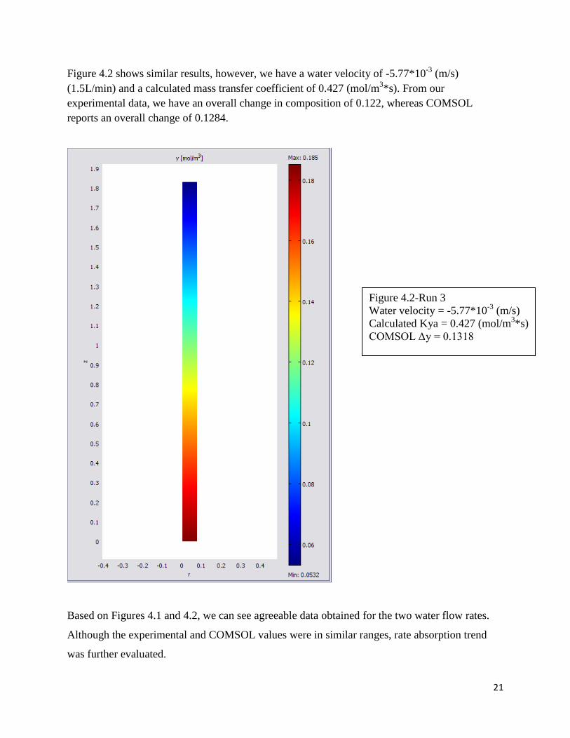
Figure 4.2 shows similar results, however, we have a water velocity of -5.77*10-3

(m/s)

(1.5L/min) and a calculated mass transfer coefficient of 0.427 (mol/m3*s). From our

experimental data, we have an overall change in composition of 0.122, whereas COMSOL

reports an overall change of 0.1284.

Based on Figures 4.1 and 4.2, we can see agreeable data obtained for the two water flow rates.

Although the experimental and COMSOL values were in similar ranges, rate absorption trend

was further evaluated.

Figure 4.2-Run 3

Water velocity = -5.77*10-3

(m/s)

Calculated Kya = 0.427 (mol/m3*s)

COMSOL Δy = 0.1318

22

Table 4.1 and Figure 4.3 both present experimental versus simulation values for the overall

change in the mole fractions for Runs 1-4.

Table 4.1: Experimental vs. COMSOL Absorption Rate

In sync with the COMSOL models, we can see that “delta y” increases as water flow rate

increases. We know from literature that the packing material in the absorption column creates a

larger contact area for liquid-gas interaction. As a result, when the liquid flow increases, more

packing is covered and there is more uniform distribution of liquid throughout the packed tower.

As flow increases, the occurrences of channeling, uneven distribution of gas or liquid flow in the

column, occurs.

Figure 4.3 Absorption Rates for Experimental & COMSOL (Runs 1-4)

Though the COMSOL values consistently report greater changes in the overall “delta y” than the

experimental, we can assume that the previously defined assumptions contribute to these

variations.

Another important relationship that is noticed occurs between the liquid flow rate and the

mass transfer coefficient. Figure 4.4 confirms that in addition to an increase in absorption rate

with flow, there is also an increase in “Kya.” This is partially due to Kya being directly

proportional to the rate of absorption. One other justification is that the liquid boundary layer

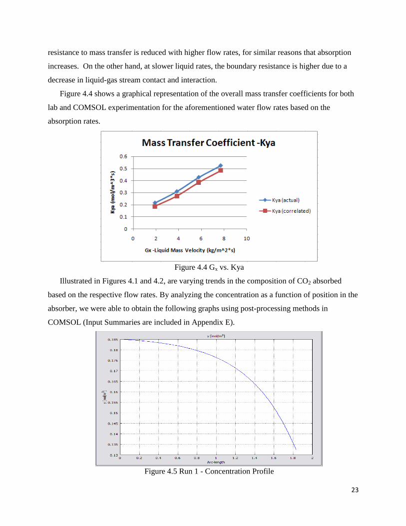
23

resistance to mass transfer is reduced with higher flow rates, for similar reasons that absorption

increases. On the other hand, at slower liquid rates, the boundary resistance is higher due to a

decrease in liquid-gas stream contact and interaction.

Figure 4.4 shows a graphical representation of the overall mass transfer coefficients for both

lab and COMSOL experimentation for the aforementioned water flow rates based on the

absorption rates.

Figure 4.4 Gx vs. Kya

Illustrated in Figures 4.1 and 4.2, are varying trends in the composition of CO2 absorbed

based on the respective flow rates. By analyzing the concentration as a function of position in the

absorber, we were able to obtain the following graphs using post-processing methods in

COMSOL (Input Summaries are included in Appendix E).

Figure 4.5 Run 1 - Concentration Profile

24

Figure 4.6 Run 3- Concentration Profile

Figure 4.5, concentration profile, for water velocity of -1.89*10-3

(m/s), illustrates an exponential

change in composition across the tower, whereas Figure 4.6, water velocity of -5.77*10-3

(m/s),

shows a more linear composition change at its respective flow rate and mass transfer coefficient.

With further study and experimentation with COMSOL, these trends can be used to analyze

carbon dioxide composition in the gas phase as a function of time inside the packed tower.

25

Liquid Phase Analysis

We can also evaluate the accuracy of COMSOL predictions based on the previous assumptions

to solve for the concentration in the liquid bottoms stream. In the post-processing used to

compare CO2 absorbed in the gas phase, we can perform the same analysis for the liquid phase.

Figure 4.7 shows the carbon dioxide in the liquid phase, with a maximum mole fraction of

1.298e-4 compared to a value of 1.3e-4 from experimental data collection.

Figure 4.7 Run 1

H2O velocity = -1.89*10-3

(m/s)

Kya = 0.214 (mol/m3*s)

COMSOL max. x = 1.298e-4

26

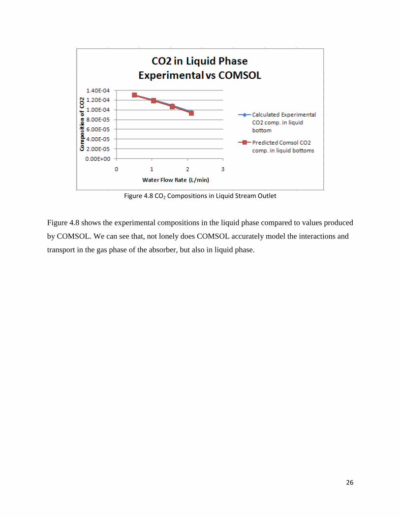
Figure 4.8 CO2 Compositions in Liquid Stream Outlet

Figure 4.8 shows the experimental compositions in the liquid phase compared to values produced

by COMSOL. We can see that, not lonely does COMSOL accurately model the interactions and

transport in the gas phase of the absorber, but also in liquid phase.

27

CONCLUSIONS

Based on our results and collected data, we can come conclude that COMSOL can be a

useful tool for predicting absorption rates given specific gas and liquid velocities, mass transfer

coefficients and a specified initial concentration.

For all four water flow rates used in the absorption lab, COMSOL approximated very well,

almost matching the change in composition at both 1.0 and 1.5 L/min water flows. We can also

use COMSOL to predict concentrations as a function of time in place inside the absorber. Given

such successful results, it can be a useful learning tool for students to use COMSOL before

performing experimental analysis. This can assist in providing an understanding of gas-liquid

interactions within a packed tower, reinforcing important concepts, and providing students with a

range of expected values for particular flow rates. If used after lab experimentation, modeling

can be used as a set of guidelines to verify values collected in the lab. COMSOL not only

provides a quantitative analysis for the packed tower, in regards to predicting amount of CO2

removed, but also a qualitative analysis, which is essential in understanding the absorption

process in its entirety.

RECOMMENDATIONS

Included in this section are two sets of recommendations that can be taken into account for

performing the gas absorption lab experiment and modeling gas absorption using COMSOL

Multiphysics and other useful software.

Gas Absorption Lab Experiment

As this was the first year using the new gas absorber in the Unit Operations (UO)

laboratory, there are several methods that can both be changed and implemented in the future.

First, more time should be allotted before measuring/recording data. In the UO lab, twenty

minutes was allowed for the system to come to equilibrium, however, the maximum absorption

for that particular liquid flow rate was not achieved. I believe that permitting an extra ten

minutes would give more accurate data. With this additional information, the CO2 in the liquid

bottoms can be analyzed. One segment of the collection procedure that was omitted from this

particular lab, was the analysis of carbon dioxide in the liquid outlet. This can be tested using the

28

carbon electrode built specifically for the gas absorber. Techniques for assembling and using the

electrode can be found in Appendix F. Another analysis tool that was not included in this years'

lab was the use of equipment software. The absorber comes with a program that can be used to

collect and record data without the use of the Rosemont Analyzer. Implementing these tools can

help produce more accurate and reliable data.

Modeling Component

There are some variations in modeling absorption with COMSOL Multiphysics. The

basis of the modeling was focused on mass transport and the Convection/Diffusion applications.

Though we only used modeling for the simplest case, a dilute system, there are applications built

for the analysis of concentrated vapors, such as the Maxwell-Stefan Diffusion and Convection

application. This particular mode allows for accurate modeling of a concentrated mixture by

setting up the proper multi-component mass transport equations. It also permits the use of up to

four species in the absorption column.

Another important segment of gas absorption that can be modeled in the future is the

mass transfer theories, specifically the two film theory. As we know. In separation processes,

materials must be diffused from one phase to another, which affect the overall mass transfer

coefficient. In the two film theory, equilibrium is assumed at the interface, and the resistances to

mass transfer in the two phases are added to an overall resistance [3]. Figure 6.1 illustrates the

assumptions made under the two film theory.

Figure 6.1 Two Film Theory (http://web.deu.edu.tr/atiksu/ana52/aedet01.gif)

29

Aspen Plus

Another useful tool that can be used for understanding absorption concepts and trends is

Aspen Plus. Aspen Plus can be used for various chemical engineering applications. For example,

it can execute tasks as simple as describing thermodynamic properties of an ethanol and water

mixture, or as complex as predicting the steady-state behavior of a full-scale petrochemical plant

[11]. Aspen is also a useful tool for simulating reaction engineering scenarios, such as designing

and sizing reactors, predicting reaction conversions, and understanding reaction equilibrium

behavior. Though this program does not create concentration profiles, it does allow for

reasonable predictions for an absorber under certain conditions. However, in order to maximize

its ability, the best way to model an absorption column would be to apply Rate-Based equations

in the Rad-Frac mode. A similar test was tried for this project. The input summary of the trial is

included in Appendix F for future study.

30

REFERENCES

[1] Wikipedia. Carbon. Retrieved October 23, 2007, from http://en.wikipedia.org/wiki/Carbon

[2] EPA. Greenhouse Gas Emissions. Retrieved March 15, 2008, from http://www.epa.gov/

[3] Cussler, E. L. (1997). Absorption. Diffusion: Mass Transfer in Fluid Systems (2nd ed. pp. 245-264). USA:

Cambridge University Press.

[4] McCabe, W. L., Smith, J. C. & Harriott, P. (2005). Unit Operations of Chemical Engineering (7th ed.).

In (E. D. Glandt, M. T. Klein & T. F. Edgar, Eds.). USA: Mc-Graw Hill.

[5] Lenntech. Lenntech: Carbon Dioxide. Retrieved March 15, 2008, from www.lenntech.com

[6] Kohl, A. L. & Neilsen, R. (1997). Gas Purification (5th ed.). USA: Gulf Professional Publishing.

[7] U.S. Department of Energy. Coal. Retrieved November 14, 2007, from http://www.energy.gov/

[8] Schifftner, K. C. (2002). Air Pollution Control Equipment Selection Guide. USA: Lewis Publishers.

[9] Douglass, D. Research Products Center. University of Wyoming. Retrieved April 22, 2008, from

http://uwadmnweb.uwyo.edu

[10] Singh, P., Niederer, J. & Versteeg, G. (April 22, 2008). Structure and activity relationships for amine

based CO2 absorbents. International Journal of Greenhouse Gas Control, 1(1). Retrieved April 22, 2008,

from http://www.sciencedirect.com/science? Science Direct-WPI George C Gordon Library.

[11] aspentech. Aspen Plus Conceptual design of chemical processes. Retrieved March 16, 2008, from

http://www.aspentech.com/products/aspen-plus.cfm

[12] Geankoplis, C. J., Transport Processes and Separation Process Principles, 4th Ed., Prentice Hall,

Upper Saddle River, NJ, (2003), p. 686.

31

APPENDIX A – GAS ABSORPTION IN A PACKED TOWER LAB

Worcester Polytechnic Institute

Department of Chemical Engineering

ChE 4402 Gas Absorption in a Packed Tower B term

Introduction and Objectives

Carbon dioxide is considered to be the largest contributor to the global warming problem. The

removal of CO2 from industrial gas streams is becoming increasingly important due to the need

to control greenhouse gas emissions to protect the environment. Carbon dioxide can be removed

from an industrial effluent gas stream by absorption into a liquid solvent. This separation

process is normally achieved in a column packed with packing materials designed to promote

direct contact between the solvent flowing downward over the packing and a continuous gas

phase flowing upward. In industrial processes, the solvent is usually an aqueous potassium

carbonate or amine solution that provides enhanced absorption through reaction with the CO2.

In this experiment you will study the absorption of CO2 from air in a packed column using water

as the solvent. The main goal is to determine the effect of gas and liquid flow rates on the

overall mass transfer coefficient for this absorption process. You will also be asked to use the

information obtained for an absorption design calculation.

Apparatus

(1) Tower

The column is a 3-inch diameter glass column partially filled with ¼ in. glass Raschig rings.

(2) Gas supply

CO2 and air are available from tanks equipped with regulators. The regulator pressure should be

set at 20 psig for each gas. Flow rates of the gases are maintained at desired levels using flow

control valves and rotameters. The gases are mixed using a specially designed mixing tube

located after the flow meters and prior to entering the bottom of the tower.

(3) Liquid supply

Water is pumped from a sump tank, through a rotameter, to the top of the column. It flows

downward through the column and can be returned back to the sump tank or diverted to the drain

using valves in the pipes below the column. If water is to be diverted to the drain, it is necessary

to open valves to provide make-up tap water to the sump tank. A float mechanism in the sump

tank will maintain a constant level in the tank as long as the appropriate valves are opened.

During column operation with gas flowing upward, a liquid seal must be maintained in the pipes

32

below the column by appropriate adjustment of the return or drain valves. That is, the rate of

water flow returned to the sump or diverted to the drain must be maintained at a rate equal to the

inlet water flow rate to maintain a constant height of water in the pipe below the column. That

way, water does not backup and flood the column and the gas entering the column at the bottom

does not escape into the sump or out the drain.

(4) Measurements

Flow rates of air, CO2 and water are obtained from rotameters. Calibration data is attached.

Thermocouples at the column top and bottom provide temperature measurements that can be

read on the column control panel. Pressure drop across each of two sections of the column can

be obtained from digital readings of differential pressure gages. A water-filled manometer

provides a measure of the difference between the pressure at the column top and atmospheric

pressure. Inlet and outlet gas CO2 compositions are measured with a Rosemount Analytical Inc.

non-dispersive infrared analyzer located in Goddard 116 on the main floor of the lab, just above

the column outlet. The Rosemount analyzer provides a digital readout of the volume percent

CO2 in the air.

Procedure

(1) Preliminary inspection of equipment

It is necessary that each student understand the arrangement and operation of the equipment

before any experimental work is undertaken. A complete inspection of the equipment should be

made and the function of each part of the apparatus should be determined. A detailed schematic

should be drawn. Each member of the lab group will be expected to answer questions about the

equipment during the lab session.

(2) Preliminary work

The Rosemount infrared spectrometer should be calibrated prior to the experiment using nitrogen

gas and two available standard CO2/air mixtures. The standard gas cylinders have regulators that

should be set at about 10-15 psig. Sample valves on a panel above the analyzer can be opened

one at a time to introduce the samples individually. A pressure of 1 inch of water at the

manometer on the panel gives suitable flow rates for gases flowing into the analyzer. The flow

control valve next to the manometer should be opened slowly to establish the flow that provides

1 inch of water. The pure nitrogen gas is used as the zero point reference. Once nitrogen is

introduced at the sample port and has been flowing for at least two minutes, press zero then

enter on the Rosemount front panel. After a minute or two, the instrument should read zero (or

nearly so). Close the flow control valve and the N2 sample valve. To calibrate the instrument

over the range from zero to 20% CO2, a 20% CO2 mixture is introduced in the sample port.

33

After this flow has been established for a minute or two by opening the flow control valve just

enough to get 1 inch of water on the manometer, press span then enter. The instrument should

read 20% (or nearly so). Close the flow control valve and the 20% sample valve. You can check

the accuracy of the instrument by recording the reading for a standard 12 % CO2 mixture.

Simply establish the flow of the 12 % mixture with the flow control valve giving a 1 inch

pressure difference at the manometer and record the Rosemount reading after it becomes steady.

Our 12 % often reads slightly higher than 12%; about 12.7%. Don’t forget to close the flow

control valve and the 12 % sample valve.

(3) Experimental conditions

Inlet gas CO2 composition should be maintained at a nearly constant value somewhere between

18 and 20 % by volume. It is recommended that the air flow be no less than 750 ml/min and no

more than 1400 ml/min. Therefore, the required CO2 flow should be between 200 and 320

ml/min. The calibration curves were obtained at 70 oF and 20 psig at the regulator. Correction

for other T and P conditions might need to be made. The water flow can be varied between 0.5

and 2.0 L/min. Inlet CO2 composition in the water entering the column can be assumed to be

zero as long as the outlet water is completely diverted to the drain. It is suggested that you study

four different water rates at a fixed gas rate during the first experimental period and that you

study the same four water rates at a different gas rate for the second experimental period. The

CO2 composition of the outlet gas stream can be monitored continuously (by opening the column

top sample valve and opening the flow control valve on the panel above the instrument just

enough to provide 1 inch of water at the manometer). It is important to wait long enough for

steady state to be achieved. It normally takes about 20 minutes for the outlet concentration to

settle to a constant value.

Theory

The engineer who is required to design an absorption tower is interested in the rate of absorption

of the material under the desired operating conditions. Considerable experimental work on a few

systems has been reported in the literature that will enable the designer to predict the effect of

certain operating variables on the rate of absorption for a given type of apparatus. The

absorption rate is generally expressed as an overall mass transfer coefficient, K, which may be

based on either a gas or a liquid-phase driving force. In most cases it is impossible to determine

the area of contact of the gas and liquid. Therefore, the coefficients are reported on a volume

basis. For dilute systems with straight operating and equilibrium lines, a design equation for the

volume of a gas absorption tower may be written as:

Lty yVaKW )( (1)

where

W = absorption rate of solute gas; mol/h

Kya = overall mass transfer coefficient based on the gas-phase driving force, mol/h/m3

Vt = gross tower volume occupied by packing, m3

Ly = logarithmic mean driving force; logarithmic mean of (yb-yb*) and (ya-ya*)

yb = mole percent CO2 in the gas phase at column bottom

34

ya = mole percent CO2 in the gas phase at column top

yb* = mole percent CO2 in the gas phase that would be in equilibrium with the liquid at column

bottom

ya* = mole percent CO2 in the gas phase that would be in equilibrium with the liquid at the

column top

The equilibirium relation for CO2 dissolved in water can be represented by Henry’s law

yCO2* P = H xCO2

Henry’s constant may be assumed to be 1400 atm at 20 oC [1].

Under certain assumptions, a design equation for the column height is given by [2]:

b

ay yy

dy

aK

SVZ

*

/ (2)

where

S = cross sectional area, m2

V = molar flow rate of the gas phase, mol/h

The integral in this equation represents the change in vapor composition divided by the average

driving force and is called the number of transfer units based on the overall gas phase driving

force, NOy. The other part of Equation 2 has units of length and is called the height of a transfer

unit based on the overall gas phase driving force, HOy. Thus the height of the column is given by:

Z = HOyNOy (3)

For dilute systems or those with otherwise straight operating and equilibrium lines, the integral

in Equation 2 is easily determined using the logarithmic mean and the number of transfer units is

given by:

L

ab

Oyy

yyN

(4)

The overall resistance to mass transfer can be considered to be made of a gas phase film

resistance and a liquid phase film resistance and the height of a transfer unit can be considered to

be made up of a contribution from the liquid film and a contribution from the gas film as given

by [3]:

xyOy H

L

VmHH (5)

where m is the slope of the equilibrium line and V and L are the average molar flow rates of the

gas and liquid. This formulation is useful for design purposes because correlations are available

for Hx and Hy. For example, Geankoplis [4] gives

35.05.05.0

678.0782.6660.0

226.0

yx

p

y

GGSc

fH (6)

and

3.0

3

5.0

)108937.0/(782.6

/

372

357.0

x

p

x

GSc

fH (7)

35

where Hx and Hy have units of meters,

Sc = Schmidt number = / ( DAB)

= viscosity

= density

DAB = diffusivity of solute A in B (gas phase for Hy and liquid phase for Hx)

fp = a relative mass transfer coefficient for a given packing material compared to a reference

packing material. fp can be assumed to be 1.5 for ¼ Raschig rings.

Gy = gas mass velocity in kg/m2s

Gx = liquid mass velocity in kg/m2s

These correlations are not generally expected to give accurate quantitative predictions, but they

should provide reasonable rough estimates and show appropriate trends in mass transfer behavior.

Note that Oy

yHS

VaK (8)

For design purposes, the height of column required to provide a specified separation can be

obtained from Equation 3, if correlations like Equations 6 and 7 are used together with

equilibrium information to estimate HOy in Equation 5. Alternatively, if the column height is

given, and an estimate is obtained for HOy, the outlet compositions that will result for given inlet

flows and compositions can be determined from Equation 3 together with a mass balance.

Equations 3 and 8 could also be used to evaluate HOy from experimental data obtained on a given

column.

Also note that mass transfer coefficients and transfer units can alternatively be based on the

liquid phase driving force and that although HOy HOx and NOy NOx design results in terms of

column heights or product stream compositions based on the two methods should be similar.

Calculations

The following calculations should be performed:

(a) a value of Kya should be calculated for each run. The value of W to be used in this

calculation should be obtained from a material balance on CO2 in the gas phase.

(b) estimates of error should be attached to any value of Kya and error bars should be provided

on all plots.

(c) Plots of Kya versus liquid mass velocity, Gx, should be made and a correlation of Kya as a

function of liquid mass velocity should be attempted. Gx should be based on the total cross

sectional area of the tower, and has units of kg/m2-h.

(d) Estimates of HOy and Kya obtained should be obtained from correlations and compared with

the experimental results, including a comparison of the expected and experimental dependence

of Kya on Gx and Gy.

Design Requirements

Determine the outlet compositions (vapor and liquid) for an absorption process at 20 oC using

our column with 2.5 L/min water flow rate to treat a 20 % CO2/air stream flowing at 2 L/min.

36

Determine how this water flow rate compares to the minimum water rate required to accomplish

the same removal of CO2 from the vapor phase.

Hint: an equation for the operating line can be determined to be [5]:

2

2

1

1

1

1

2

2

1'

1'

1'

1'

y

yV

x

xL

y

yV

x

xL

where L’ and V’ are the CO2 free water and air molar flow rates, respectively.

For the case where x2 = 0 (pure water entering at column top), the operating line can be plotted

as [6]:

2

2

2

2

11'

'1

11'

'

)(

y

y

x

x

V

L

y

y

x

x

V

L

xy

where y2 is the mole fraction of CO2 in the gas exiting the top of the column.

Results and Discussion

A discussion of the errors in the results due to experimental uncertainty and their effect on the

results through propagation of error should be included. How meaningful are your results when

errors are considered. It is not sufficient to simply state your results in numerical form. They

should be interpreted in terms of physical phenomena occurring within the process. Do the

trends in the data make sense? Do your results agree with published information or correlations?

What is happening physically inside the column when the water rate is changed that can account

for the observed dependence of the mass transfer coefficient on the water rate?

Report Requirements

The pre-lab report should contain an introduction stating the objective of the experiments,

including the rationale for expecting Kya to depend on the liquid flow rate, some background on

gas absorption, a detailed derivation of the design equation from first principles, including the

assumptions and simplifications made, a description of the equipment and purpose of each item,

including a detailed schematic drawing, and a stepwise procedure, that would allow someone

who is unfamiliar with the equipment to perform the experiment. Following the first week of

experiments, calculations of Kya for all liquid flow rates should be made and correlated against

Gx.

These results are to be presented informally to the instructor before the second week’s

experiments. Error analysis is not required at this stage. The final report should contain the

usual sections as specified in the course descriptions. In addition, an error analysis is required

for all calculated values of Kya, and error bars are to be included on all plots.

37

Calibration Curves

A calibration curve for the digital water flow meter is provided in Figure 1. Note that the

measured water flow was 2.1 L/min when the meter read 2.0 L/min. Figures 2 and 3 show

calibration curves for air and CO2 rotameters, respectively. Note that the float travel is measured

at the center of the float. Equations for best fit lines provided on these curves should not be

extrapolated beyond the ranges shown.

y = 1.062x - 0.015

R2 = 0.9994

0

0.5

1

1.5

2

2.5

0 0.5 1 1.5 2 2.5

Meter Reading (L/min)

Me

as

ure

d F

low

(L

/min

)

Linear

Figure 1. Calibration curve for absorption column water flow meter.

y = 8.9764x + 72.438

R2 = 0.9981

0

200

400

600

800

1000

1200

1400

1600

0 50 100 150 200

Float Travel (center of float)

Air

Flo

w (

ml / m

in)

Linear

Figure 2. Calibration curve for absorption column air rotameter.

38

y = 8.6783x + 98.395

R2 = 0.9998

0

100

200

300

400

500

600

0 10 20 30 40 50 60

Float Travel (center of float)

CO

2 F

low

(m

l /

min

)

Linear

Figure 3. Calibration curve for absorption column CO2 rotameter.

References

1. McCabe, W. L., Smith, J. C., and Harriott, P., Unit Operations of Chemical Engineering, 7th

Ed., McGraw-Hill, New York, (2005), p. 580.

2. Ibid, p. 581.

3. Ibid, p. 584.

4. Geankoplis, C. J., Transport Processes and Separation Process Principles, 4th

Ed., Prentice

Hall, Upper Saddle River, NJ, (2003), p. 686.

5. Ibid, p. 665.

6. Cussler, E. L., Diffusion: Mass Transfer in Fluid Systems, 2nd

Ed., Cambridge University

Press, NY, (1997), p. 260.

39

APPENDIX B – LAB CALCULATIONS Calculating Volumetric and Molar Flows

Note: Calculations for conversions into molar flow rate are only given for one species.

Conversions for the other species were calculated using the identical formats.

CO2 (L/min) entering column (Correlation given in Absorption Lab Appendix _):

3153525.01000/)395.98)25*6783.8(

CO2 (mol/hr) entering column:

8512583.060*1000*)01.44

1(**)3^10*3153525.0( 2 CO

where )/(98.1 3

2 mkgCO

Amount of CO2 coming out of the system:

)1/(min))/(*( aa yLAirflowy

min))/(419198.1(__2

_2

Lx

x

outAiroutCO

outCOya

232953.)141.1(

200107.0min))/(419198.1(141.0

xLx

Amount of CO2 absorbed:

)/(_2)/(_2 hrmoloutCOhrmolinCO

222427.0628831.08512583.0

Amount of CO2 in liquid:

)/(

]*)_2)/([(]*))/(_2)/([(

hrmolWaterFlow

yaoutCOhrmolAirFlowyhrmolinCOhrmolAirFlowx b

b

000132838.009101.1718/]141.0*)232953.0523526069.3[(]186.0*)8512583.0523526069.3[(

Concentration of CO2 in entering gas phase:

40

185973.0*1400 xbby

Logarithmic mean driving force:

0164674.0

]ln[

)]()[(

ayya

byyb

ayyabyybyL

Number of Transfer Units:

73266.2

yL

yNoy

Liquid mass velocity:

)/1(*)3600/1(*)1000/1(** 2 SMWWaterflowGx OH

885813.1)004560367.0/1(*)3600/1(*)1000/1(*02.18*09101.1718

Gas Mass Velocity:

008506077.0004560367.0

)3600/1(*)/(

hrkgGasflowGy

Gas phase film resistance:

074412.0678.0782.6660.0

226.035.05.05.0

GyGxScy

fHy

p

Liquid phase film resistance:

198482983.0)108937.0(782.6372

357.03.0

3

5.0

GxScx

fHx

p

Schmidt number (Sc):

ABDSc

25.556)10*6.1(*1000

10*9.89

4

Scx

41

959375.0)10*6.1(*2.1

10*842.15

5

Scy

Height of a Transfer Unit:

669238.073266.2

8288.1

Noy

ZHoy

Mass Transfer Coefficient:

429134.1433)669238.0)(004560367.0(

3747844.4

*

HoyS

VaK y

Rate of Absorption:

19687.001647.0)00834.0(43.1433)( yLVaKW ty

42

APPENDIX C – MODEL CONVERSIONS/CALCULATIONS

Note: COMSOL reports velocity in m/s, so values calculated from the lab portion of this project

were further converted to fit into the model properly.

Velocity of gas:

Velocity of liquid:

Initial concentration of CO2:

Note: COMSOL accepts concentration in units of (mol/m3), unlike our reported concentrations

from the absorption lab which were without units. As a result, the following conversions must be

done.

CO2 in gas and liquid phases:

Reaction Rate:

43

APPENDIX D-EXCEL SHEET (EXPERIMENTAL DATA)

44

APPENDIX E – COMSOL MODEL SUMMARY

Table of Contents

Title - COMSOL Model Report Table of Contents Model Properties Constants Global Expressions Geometry Geom1 Solver Settings Postprocessing Variables

Model Properties

Property Value

Model name

Author

Company

Department

Reference

URL

Saved date Apr 23, 2008 5:42:22 PM

Creation date Apr 22, 2008 9:09:40 PM

COMSOL version COMSOL 3.4.0.248

File name: R:\MQP\absorber1actualfinal.mph

Application modes and modules used in this model:

Geom1 (Axial symmetry (2D)) o Convection and Diffusion (Chemical Engineering Module) o Convection and Diffusion (Chemical Engineering Module)

Constants

Name Expression Value Description

D1 1.6e-5 diffusivity of CO2 in air

D2 1.6e-9 diffusivity of CO2 in water

v1 (1.419+.315)*(1/1000)*(1/60)*(1/0.00456) velocity of gas

45

v2 -(0.516)*(1/1000)*(1/60)*(1/0.00456) velocity of water

c10 0.185*101325/8.314/298 initial concentration of CO2 in gas

c20 0 inital concentration of CO2 in water

Kya 770.067/3600 calculated mass transfer coefficient

Ke 1400 equilibrium constant (atm)

Global Expressions

Name Expression Unit Description

y c1*8.314*298/101325 mol/m^3 mol fraction in gas phase

x c2*1000/55.55/100^3 mol/m^3 mol fraction in liquid phase

Geometry

Number of geometries: 1

Geom1

Point mode

46

Boundary mode

Subdomain mode

47

Geom1

Space dimensions: Axial symmetry (2D)

Independent variables: r, phi, z

Mesh

Mesh Statistics

Number of degrees of freedom 4126

Number of mesh points 550

Number of elements 964

Triangular 964

Quadrilateral 0

Number of boundary elements 134

Number of vertex elements 4

Minimum element quality 0.714

Element area ratio 0.234

Application Mode: Convection and Diffusion (chcd)

Application mode type: Convection and Diffusion (Chemical Engineering Module)

Application mode name: chcd

Application Mode Properties

48

Property Value

Default element type Lagrange - Quadratic

Analysis type Stationary

Equation form Non-conservative

Equilibrium assumption Off

Frame Frame (ref)

Weak constraints Off

Constraint type Ideal

Variables

Dependent variables: c1

Shape functions: shlag(2,'c1')

Interior boundaries not active

Boundary Settings

Boundary 4 1 2

Type Insulation/Symmetry Axial symmetry Concentration

Concentration (c0) mol/m3 0 c10 c10

Boundary 3

Type Convective flux

Concentration (c0) mol/m3 0

Subdomain Settings

Subdomain 1

Diffusion coefficient (D)

m2/s D1

Reaction rate (R) mol/(m3⋅s) -Kya*(c1*8.314*298/101325-Ke*c2*1000/55.55/100^3)

z-velocity (v) m/s v1

Subdomain initial value 1

Concentration, c1 (c1) mol/m3 c20

Application Mode: Convection and Diffusion (chcd2)

Application mode type: Convection and Diffusion (Chemical Engineering Module)

Application mode name: chcd2

49

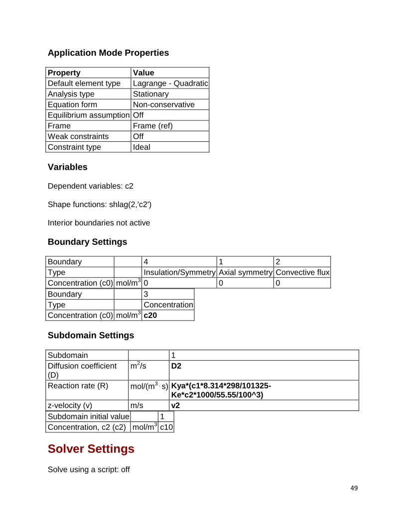
Application Mode Properties

Property Value

Default element type Lagrange - Quadratic

Analysis type Stationary

Equation form Non-conservative

Equilibrium assumption Off

Frame Frame (ref)

Weak constraints Off

Constraint type Ideal

Variables

Dependent variables: c2

Shape functions: shlag(2,'c2')

Interior boundaries not active

Boundary Settings

Boundary 4 1 2

Type Insulation/Symmetry Axial symmetry Convective flux

Concentration (c0) mol/m3 0 0 0

Boundary 3

Type Concentration

Concentration (c0) mol/m3 c20

Subdomain Settings

Subdomain 1

Diffusion coefficient (D)

m2/s D2

Reaction rate (R) mol/(m3⋅s) Kya*(c1*8.314*298/101325-Ke*c2*1000/55.55/100^3)

z-velocity (v) m/s v2

Subdomain initial value 1

Concentration, c2 (c2) mol/m3 c10

Solver Settings

Solve using a script: off

50

Analysis type Stationary

Auto select solver On

Solver Stationary

Solution form Automatic

Symmetric auto

Adaption Off

Direct (UMFPACK)

Solver type: Linear system solver

Parameter Value

Pivot threshold 0.1

Memory allocation factor 0.7

Stationary

Parameter Value

Linearity Automatic

Relative tolerance 1.0E-6

Maximum number of iterations 25

Manual tuning of damping parameters Off

Highly nonlinear problem Off

Initial damping factor 1.0

Minimum damping factor 1.0E-4

Restriction for step size update 10.0

Advanced

Parameter Value

Constraint handling method Elimination

Null-space function Automatic

Assembly block size 5000

Use Hermitian transpose of constraint matrix and in symmetry detection Off

Use complex functions with real input Off

Stop if error due to undefined operation On

Store solution on file Off

Type of scaling Automatic

Manual scaling

Row equilibration On

51

Manual control of reassembly Off

Load constant On

Constraint constant On

Mass constant On

Damping (mass) constant On

Jacobian constant On

Constraint Jacobian constant On

Postprocessing

52

APPENDIX F – ASPEN PLUS INPUT SUMMARY

RATE FRAC- MODELING ABSORPTION

;Input Summary created by Aspen Plus Rel. 20.0 at 12:46:26 Thu Apr 24, 2008

;Directory R:\Aspen Files\MQP Filename C:\DOCUME~1\yjackson\LOCALS~1\Temp\e\~ap3.tmp

TITLE 'Gas Absorption 1'

IN-UNITS MET VOLUME-FLOW='cum/hr' ENTHALPY-FLO='Gcal/hr' &

HEAT-TRANS-C='kcal/hr-sqm-K' PRESSURE=bar TEMPERATURE=C &

VOLUME=cum DELTA-T=C HEAD=meter MOLE-DENSITY='kmol/cum' &

MASS-DENSITY='kg/cum' MOLE-ENTHALP='kcal/mol' &

MASS-ENTHALP='kcal/kg' HEAT=Gcal MOLE-CONC='mol/l' &

PDROP=bar

DEF-STREAMS CONVEN ALL

SIM-OPTIONS ATM-PRES=1.01325

DESCRIPTION "

General Simulation with Metric Units :

C, bar, kg/hr, kmol/hr, Gcal/hr, cum/hr.

Property Method: None

Flow basis for input: Mole

Stream report composition: Mole flow

"

DATABANKS PURE20 / AQUEOUS / SOLIDS / INORGANIC / &

NOASPENPCD

PROP-SOURCES PURE20 / AQUEOUS / SOLIDS / INORGANIC

COMPONENTS

53

CARBO-01 CO2 /

WATER H2O /

AIR AIR

FLOWSHEET

BLOCK ABSORBER IN=LIQ-IN GAS-IN OUT=GAS-OUT LIQ-OUT

PROPERTIES NRTL

STREAM GAS-IN

SUBSTREAM MIXED TEMP=300. <K> PRES=20. <psig> &

MOLE-FLOW=4.37 <mol/hr>

MOLE-FLOW CARBO-01 0.85 <mol/hr> / WATER 0. <mol/hr> / &

AIR 3.52 <mol/hr>

STREAM LIQ-IN

SUBSTREAM MIXED TEMP=300. <K> PRES=1. <atm> &

MOLE-FLOW=1718.09 <mol/hr>

MOLE-FLOW CARBO-01 0. <mol/hr> / WATER 1718.09 <mol/hr> / &

AIR 0. <mol/hr>

BLOCK ABSORBER RATEFRAC

PARAM NCOL=1 TOT-SEGMENT=6

COL-CONFIG 1 6 CONDENSER=NO REBOILER=NO

PACK-SPECS 1 1 6 HTPACK=4.5 <ft> PACK-ARRANGE=RANDOM &

PACK-TYPE=RASCHIG PACK-MAT=GLASS PACK-DIM="8-MM" &

PACK-SIZE=8.00100E-3 SPAREA=6.290000 PACK-TENSION=73.00000 &

COL-DIAM=3. <in> VOID-FRACTIO=0.704

FEEDS LIQ-IN 1 1 / GAS-IN 1 7 ABOVE-SEGMENT

54

PRODUCTS GAS-OUT 1 1 V / LIQ-OUT 1 6 L

P-SPEC 1 1 1. <atm>

COL-SPECS 1 MOLE-RDV=1.0 Q1=0.0 QN=0.0

RAD-FRAC –MODELING ABSORPTION

INPUT SUMMARY CREATED BY ASPEN PLUS REL. 20.0 AT 12:53:09 THU APR 24, 2008

;DIRECTORY R:\ASPEN FILES\MQP FILENAME

C:\DOCUME~1\YJACKSON\LOCALS~1\TEMP\E\~AP6.TMP

;TITLE 'GAS ABSORPTION 2'

IN-UNITS MET VOLUME-FLOW='CUM/HR' ENTHALPY-FLO='GCAL/HR' &

HEAT-TRANS-C='KCAL/HR-SQM-K' PRESSURE=BAR TEMPERATURE=C &

VOLUME=CUM DELTA-T=C HEAD=METER MOLE-DENSITY='KMOL/CUM' &

MASS-DENSITY='KG/CUM' MOLE-ENTHALP='KCAL/MOL' &

MASS-ENTHALP='KCAL/KG' HEAT=GCAL MOLE-CONC='MOL/L' &

PDROP=BAR

DEF-STREAMS CONVEN ALL

DESCRIPTION "

GENERAL SIMULATION WITH METRIC UNITS :

C, BAR, KG/HR, KMOL/HR, GCAL/HR, CUM/HR.

PROPERTY METHOD: NONE

FLOW BASIS FOR INPUT: MOLE

STREAM REPORT COMPOSITION: MOLE FLOW

"

DATABANKS PURE20 / AQUEOUS / SOLIDS / INORGANIC / &

55

NOASPENPCD

PROP-SOURCES PURE20 / AQUEOUS / SOLIDS / INORGANIC

COMPONENTS

CARBO-01 CO2 /

WATER H2O /

AIR AIR

HENRY-COMPS HC-1 CARBO-01 AIR

FLOWSHEET

BLOCK ABSORBER IN=LIQ-IN GAS-IN OUT=GAS-OUT LIQ-OUT

PROPERTIES RK-ASPEN

PROPERTIES NRTL

PROP-DATA HENRY-1

IN-UNITS MET VOLUME-FLOW='CUM/HR' ENTHALPY-FLO='GCAL/HR' &

HEAT-TRANS-C='KCAL/HR-SQM-K' PRESSURE=BAR TEMPERATURE=C &

VOLUME=CUM DELTA-T=C HEAD=METER MOLE-DENSITY='KMOL/CUM' &

MASS-DENSITY='KG/CUM' MOLE-ENTHALP='KCAL/MOL' &

MASS-ENTHALP='KCAL/KG' HEAT=GCAL MOLE-CONC='MOL/L' &

PDROP=BAR

PROP-LIST HENRY

BPVAL CARBO-01 WATER 159.8650745 -8741.550000 -21.66900000 &

1.10259000E-3 -.1500000000 79.85000000 0.0

STREAM GAS-IN

SUBSTREAM MIXED TEMP=25. PRES=1. MOLE-FLOW=4.37 <MOL/HR>

MOLE-FLOW CARBO-01 0.85 <MOL/HR> / WATER 0. <MOL/HR> / &

56

AIR 3.52 <MOL/HR>

STREAM LIQ-IN

SUBSTREAM MIXED TEMP=25. PRES=1. <ATM> &

MOLE-FLOW=3000. <MOL/HR>

MOLE-FLOW CARBO-01 0. <MOL/HR> / WATER 3000. <MOL/HR> / &

AIR 0. <MOL/HR>

BLOCK ABSORBER RADFRAC

PARAM NSTAGE=2

COL-CONFIG CONDENSER=NONE REBOILER=NONE

RATESEP-ENAB CALC-MODE=RIG-RATE

FEEDS LIQ-IN 1 ABOVE-STAGE / GAS-IN 2 ON-STAGE

PRODUCTS GAS-OUT 1 V / LIQ-OUT 2 L

P-SPEC 1 1.

COL-SPECS

PACK-RATE 1 1 1 RASCHIG VENDOR=GENERIC PACK-MAT=CERAMIC &

PACK-SIZE="0.25-IN" PACK-FAC=5250.000 SPAREA=7.100000 &

VOIDFR=0.62 STICH1=48. STICH2=8. STICH3=2. HETP=2. <FT> &

DIAM=3. <IN> P-UPDATE=NO

PACK-RATE2 1 RATE-BASED=YES LIQ-FILM=FILMRXN VAP-FILM=FILMRXN &

MTRFC-CORR=ONDA-68 INTFA-CORR=ONDA-68 &

PACKING-SIZE=6.35000E-3

PACK-RATE 2 2 2 RASCHIG VENDOR=GENERIC PACK-MAT=CERAMIC &

PACK-SIZE="0.25-IN" PACK-FAC=5250.000 SPAREA=7.100000 &

VOIDFR=0.62 STICH1=48. STICH2=8. STICH3=2. HETP=31. <IN> &

57

DIAM=3. <IN> P-UPDATE=NO