Modeling Flash Floods in Small Ungaged Watersheds using ...

________________________________________________________________________

Modeling Flash Floods in Small Ungaged Watersheds using Embedded GIS

Ethan W. Knocke ________________________________________________________________________

Masters Thesis Research in Partial Fulfillment of the

Requirements for the Degree of Masters of Science in Geography

Virginia Polytechnic Institute and State University

Dr. Laurence W. Carstensen Jr., Chair Dr. David F. Kibler

Dr. Conrad D. Heatwole

January 27, 2006 Blacksburg, VA, USA

Key Words: Flash Flood, Hydrologic Modeling, Rainfall, GIS

Modeling Flash Floods in Small Ungaged Watersheds using Embedded GIS Ethan W. Knocke

ABSTRACT

Effective prediction of localized flash flood regions for an approaching rainfall

event requires an in-depth knowledge of the land surface and stream characteristics of the

forecast area. Flash Flood Guidance (FFG) is currently formulated once or twice a day at

the county level by River Forecast Centers (RFC) in the U.S. using modeling systems that

contain coarse, generalized land and stream characteristics and hydrologic runoff

techniques that often are not calibrated for the forecast region of a given National

Weather Service (NWS) office. This research investigates the application of embedded

geographic information systems (GIS) modeling techniques to generate a localized flash

flood model for individual small watersheds at a five minute scale and tests the model

using historical case storms to determine its accuracy in the FFG process. This model

applies the Soil Conservation Service (SCS) curve number (CN) method and synthetic

dimensionless unit hydrograph (UH), and Muskingum stream routing modeling technique

to formulate flood characteristics and rapid update FFG for the study area of interest.

The end result of this study is a GIS-based Flash Flood Forecasting system for

ungaged small watersheds within a study area of the Blacksburg NWS forecast region.

This system can then be used by forecasters to assess which watersheds are at higher risk

for flooding, how much additional rainfall would be needed to initiate flooding, and when

the streams of that region will overflow their banks. Results show that embedding these

procedures into GIS is possible and utilizing the GIS interface can be helpful in FFG

analysis, but uncertainty in CN and soil moisture can be problematic in effectively

simulating the rainfall-runoff process at this greatly enhanced spatial and temporal scale.

Acknowledgements

I would first like to thank each of my committee members for their guidance and

support in pursuing this research. This thesis topic pulled from many fields that I enjoy

and I appreciate all of your time, patience, and common interest in piecing together this

coupled meteorology and hydrology model in GIS.

To my advisor Dr. Carstensen, I thoroughly enjoyed attaining an advanced

knowledge in GIS analysis, application, and customization in your courses and

throughout this research process. Your GIS insight was instrumental in helping me to

construct this FFG application. Dr. Kibler, thank you for helping me to understand the

underlying hydrology involved in flash flood modeling and for all of your input and

advice in tackling FFG development at these small scales. Dr. Heatwole, thank you for

your guidance in proper application of GIS for hydrologic analysis and for your

assistance in conceptualizing this model.

There are two additional faculty members to acknowledge for assistance in related

research: Dr. Kolivras in an independent study of flash flood perception and Dr. Prisley

in a course project addressing elevation uncertainty in flood modeling.

Very special thanks to Stephen Keighton and Paul Jendrowski of the Blacksburg

NWS for their time and support in research topic development, in case storm event

selection, in determining necessary FFG improvements, and for providing critical data.

Next I would like to thank the Center for Geospatial Information Technology

(CGIT) for their financial support through research assistantships during my two years of

school. Finally I need to thank my family and friends for their motivational support and

for helping me to stay focused throughout my graduate school experience.

Ethan Knocke Acknowledgements iii

Table of Contents List of Tables v List of Figures vi List of Equations vii 1.0 Introduction 1 1.1 Problem Statement 1 1.2 Objectives 3 1.3 Study Area 4 2.0 Literature Review and Background 6 2.1 Flash Floods 6 2.2 Hydrologic Modeling 9 2.3 Flash Flood Guidance (FFG) 14 2.4 Current National Weather Service (NWS) FFG 15 2.5 Geographic Information Systems (GIS) 19 2.6 Model Architecture 21 2.7 Use of GIS in Hydrologic Modeling 22 2.8 Review of Current Flood Related Hydrologic Models 24 2.9 Issues of Scale and Resolution in Hydrologic Modeling 28 2.10 Soil Conservation Service (SCS) Curve Number (CN) Methodology 30 2.11 SCS Synthetic Unit Hydrograph (UH) 32 2.12 Muskingum Stream Routing 32 2.13 Application of Literature 33 3.0 Methodology 35 3.1 Embedded FFG Model 35 3.2 Model Implementation 46 3.3 Model Improvements to FFG System 49 3.4 Model Assumptions 50 3.5 Data Sources and Development 52 3.6 Storm Events 58 3.7 Discussion of Model Parameters 59 3.8 Model Sensitivity 64 4.0 Results 68 4.1 Elevation Sensitivity 68 4.2 Antecedent Moisture Condition (AMC) Sensitivity 74 4.3 Muskingum Verification 88 4.4 Model Interface 91 5.0 Discussion and Conclusions 101 5.1 Achievement of Objectives 101 5.2 Conclusions 105 5.3 Future Research 108 References 111 Vita 116

Ethan Knocke Table of Contents iv

List of Tables 1 – Residential Contents Protected with Warning 9 2 – A Typology of Models 24 3 – CN Classifications 37 4 – AMC Classifications 37 5 – Polynomial CN Adjustment Equations 39 6 – Ratios for Dimensionless Unit Hydrograph 40 7 – Case Storm Events 59 8 – Elevation Error Sensitivity Sample Results 70 9 – Literature Simulation Results for Ten Case Storm Events 75 10 – Accuracy Assessment of AMC Sensitivity Simulations 87 11 – Muskingum Stream Routing Inflow/Outflow Volume Comparison 89

Ethan Knocke List of Tables v

List of Figures 1 – RFC 3-hour FFG Map 2 2 – Ungaged Small Watershed Study Area for this Research 5 3 – Flood Timeline 8 4 – Diagram Describing the General Flood Hydrograph Simulation Process 12 5 – Rainfall-Runoff Curve used to compute FFG 17 6 – Polynomial CN Adjustment Curves 38 7 – Dimensionless Unit Hydrograph and Mass Curve 40 8 – FFG Model Flowchart 48 9 – Map of Watershed and Stream Data 53 10 – Map of Elevation Data 54 11 – Map of Land Cover Data 55 12 – Map of Hydrologic Soil Data 56 13 – Sample Rainfall Input Text File Generated by AMBER 57 14 – Shawsville USGS Streamgage File 58 15 – Elevation Error Grid Generation 66 16 – AMC Adjustments used in Sensitivity Analysis for CN = 50 67 17 – Watershed Delineations 68 18 – Stream Delineations 69 19 – UH Curves (Upstream Watershed) 71 20 – UH Curves (Confluence Watershed) 71 21 – UH Curves (Weak Boundary Watershed) 72 22 – Hydrographs for July 1, 2003 Storm (1600 – 1200 UTC) 76 23 – Hydrographs for July 6, 2003 Storm (1500 – 0000 UTC) 77 24 – Hydrographs for September 18, 2003 Storm (1600 – 0600 UTC) 78 25 – Hydrographs for November 19, 2003 Storm (0600 – 0000 UTC) 79 26 – Hydrographs for April 13, 2004 Storm (0600 – 0000 UTC) 81 27 – Hydrographs for September 8, 2004 Storm (0000 – 1630 UTC) 82 28 – Hydrographs for September 17, 2004 Storm (0600 – 0000 UTC) 83 29 – Hydrographs for September 28, 2004 Storm (0000 – 1600 UTC) 84 30 – Hydrographs for November 24, 2004 Storm (1000 – 0600 UTC) 85 31 – Hydrographs for January 14, 2005 Storm (1000 – 0300 UTC) 86 32 – Inflow and Outflow Hydrograph Comparison for Short Routing Reach 89 33 – Inflow and Outflow Hydrograph Comparison for Long Routing Reach 90 34 – Inflow and Outflow Hydrograph Comparison for Outlet Routing Reach 90 35 – Rainfall Distribution Interface 92 36 – Accumulative Rainfall Interface 93 37 – Precipitation Excess Interface 94 38 – Initial Abstraction Rainfall Interface 95 39 – Runoff CN Interface 96 40 – Stream Discharge Interface 97 41 – Flash Flood Risk Interface 99 42 – FFG Interface 100

Ethan Knocke List of Figures vi

List of Equations 2.1 – Threshold Runoff Equation 17 3.1 – Rainfall-Runoff Equation (SCS-CN) 36 3.2 – Curve Number Equation (SCS-CN) 36 3.3 – Initial Abstraction Equation (SCS-CN) 36 3.4 – Normal AMC CN Adjustment Equation 38 3.5 – Dry AMC CN Adjustment Equation 38 3.6 – Wet AMC CN Adjustment Equation 38 3.7 – Basin Lag Time Equation (SCS UH) 39 3.8 – Time to Peak Discharge Equation (SCS UH) 39 3.9 – Peak Discharge Equation (SCS UH) 39 3.10 – Stream Routing Equation (Muskingum) 42 3.11 – First Routing Coefficient Equation (Muskingum) 42 3.12 – Second Routing Coefficient Equation (Muskingum) 42 3.13 – Third Routing Coefficient Equation (Muskingum) 42 3.14 – Travel Time Equation 42 3.15 – Bankfull Velocity Equation 43 3.16 – Two-Year Flow Regression Equation 43 3.17 – Channel Width Regression Equation 43 3.18 – Channel Depth Regression Equation 43

Ethan Knocke List of Equations vii

1.0 Introduction

1.1 Problem Statement

Flash floods can develop rapidly in local areas with little or no warning. These

weather-related natural disasters can occur at any time within regions regardless of

whether or not they have a stream gage to monitor stream levels. Flash flood events can

cause many deaths and millions of dollars in property damage if the public is not warned

in advance. When flash flood conditions become likely or imminent, the public needs to

be warned in an informative and timely manner to minimize these impacts. This warning

process includes the recognition of precipitation onset, the collection and evaluation of

data by human analysts or automated systems, threat recognition, notification, decision

generation, response activation, and public action and mitigation strategies (Carsell,

2004).

The current National Weather Service (NWS) Flash Flood Guidance (FFG) model

is developed and distributed once or twice a day by thirteen River Forecast Centers

(RFCs) using a variety of hydrologic modeling techniques at varying scales. These

techniques can be problematic and error prone on localized scales and in ungaged

locations and output is provided on a very coarse, inconsistent, and uninformative county

scale (Carpenter et. al., 1999, RFC, 2003). Figure 1 provides a clear picture of the

downfalls of the current model output due to the high spatial variation in FFG

categorization:

Ethan Knocke Chapter 1 - Introduction 1

Figure 1 – RFC 3-hour FFG Map (RFC, 2003 pg. 38)

This method of distributing FFG to forecasters, who use the guidance to

determine and warn of flash flood occurrence, needs improvement because of issues

involved with:

• the loosely coupled framework to which the FFG functions,

• the untimely fashion that FFG values update,

• the generalized inconsistent scale to which guidance is portrayed, and

• the lack of technological advancement to incorporate the improved spatial

analysis and data structures that are available in current GIS.

GIS is used to analyze and describe the spatial environment through analytical

functions and a spatial data structure, while hydrologic modeling simulates the

functionality and evolution of hydrological processes using mathematics and governing

hydrologic equations (Maidment, 1996). These simulations require input data about the


watersheds within which these processes occur and require analytical tools to perform the

mathematics necessary to answer the governing equations. The strong relationships

between the two frameworks make it possible to embed a hydrologic model within the

GIS framework using object oriented programming languages to express and quantify the

hydrological equations and analysis techniques necessary to simulate processes.

Hydrological modeling has been widely associated with GIS for applications in water

quality, nonpoint pollution, erosion, and flooding (Brimicombe et. al., 1996). The use of

GIS in flood modeling and mitigation specifically has focused on hydrological modeling

and graphical visualization and communication of flood hazard information.

The purpose of this research is to investigate embedding lumped hydrologic

modeling techniques into a GIS for generation of localized real-time FFG in ungaged

small sub-watershed regions that can then be used as a supplement for flash flood hazard

identification and communication. The basic research objective is to contribute to the

advancement of methodologies involved in FFG development by addressing an applied

research objective investigating ways in which embedded GIS modeling and analysis can

enhance the accuracy of flash flood modeling techniques.

1.2 Objectives

The three primary objectives associated with this embedded FFG research are to:

• investigate the ways in which embedded GIS modeling and analysis can enhance

the accuracy of ungaged small sub-watershed hydrologic modeling techniques by

using a set of hydrograph procedures to develop a runoff response model within

the GIS framework


• test the effect that required input parameters for the hydrological formulas have

on the resulting FFG output, using sensitivity analyses

• advance the methodologies involved in real-time FFG development by

performing statistical analyses on the results of the most accurate FFG output

The unit of analysis for these objectives will be 35 small watersheds within the

South Fork of the Roanoke River, and the level of measurement for the output FFG will

be ratio, a zero based numerical score of rainfall requirements for flash flood generation.

This will dramatically improve both the spatial and temporal detail of the FFG, and will

provide much needed information for flood forecasters and the general public. It is

believed that these objectives will lead to the generation of a more accurate GIS-

embedded hydrological FFG modeling approach because it will utilize proven hydrologic

formulas and theories that can work for any watershed or sub-watershed and will

incorporate more detailed modeling parameters that can be generated within the GIS

framework. Observing the computational sensitivity of a few of the input parameters in

this GIS model will reveal the optimal FFG technique from this research, and potentially

make flash flood monitoring an easier task to undertake.

1.3 Study Area

Criteria for selection of the study area in this research included the following:

• Must be within the NWS Blacksburg forecast area for future application

• Must be in a headwater region where flash flooding occurs most frequently

• Must contain a sufficient number of small ungaged sub-watersheds

• Must drain into an outlet that contains a real-time stream gage


• Must contain complex terrain to incorporate topographic effects

• Must contain a mixture of land cover and soil groups to incorporate their effects

The South Fork of the Roanoke River was selected as a study area because: this is

a headwater section of the Roanoke River basin, the region includes 35 ungaged sub-

watersheds ranging in size from 0.5 to 9.5 square miles, the outlet of this stream network

contains a USGS stream gage in Shawsville, Virginia, there is a 2,550 foot elevation

differential between the upper headwater locations and the outlet, and there is enough

spatial variability in land and soil characteristics. Another interesting attribute of this

study area is that it is right at the border of the Ohio and the Southeast RFC coverage

areas. Figure 2 is a map of the location of this study area that includes sub-watershed

boundaries, stream network, elevation, and the stream gage location.

Figure 2 – Ungaged Small Watershed Study Area for this Research Data Sources: (NWS, 2004), (USGS, 2004)


2.0 Literature Review and Background

2.1 Flash Floods

Floods are responsible for more deaths than any other weather-related

phenomenon. The 30-year average for flood-related fatalities is around 120 per year,

with most of these due to flash floods. Flash floods are incredibly dangerous natural

disasters that occur quite frequently within the United States. In fact, from 1996 to 2003

there was an average of 3000 flash flood events recorded per year nationwide. For

comparison, there were only about 1000 tornadoes annually within this same time period

(NRC, 2005).

According to the National Weather Service (NWS), a flood is the inundation of a

normally dry area caused by an increase in water level within rivers, streams, or drainage

ditches (NWS, 2005). A flash flood is an event in which sections of a water body rapidly

rise out of their banks within six hours of a rainfall event (Sweeney, 1992). They

typically develop within storm events that contain brief periods (on the order of minutes

to hours) of intense rainfall over a given watershed region. Key ingredients for rainfall

events that can lead to flash floods include (NRC, 2005):

• Ample and persistent supply of water vapor

• A mechanism for uplift of air to condense the moisture into clouds and

precipitation (convection, orographic lifting, boundaries)

• A focusing mechanism that enhances the precipitation and can cause it to occur

continuously and repeatedly over the same area (fronts, boundaries, lows)

Ethan Knocke Chapter 2 – Literature Review and Background 6

The most common events that generate flash flood conditions are frontal systems,

tropical systems, multi-cell convection, supercell convection, squall lines, and derechoes,

and other mesoscale convective systems (Dowsell III, 1995). Events such as rapid

snowmelt, dam failure, levee system failure, or prior long-duration low intensity rainfall

can combine together with these short-duration high intensity rainfall events to enhance

flood conditions (Pilgrim et. al., 1993).

Flash floods stem from a complex interaction between meteorological and

hydrological processes at varying spatial and temporal scales. Sole use of theoretical or

modeling approaches can only provide generalized estimates of flash flood potential

within a watershed network. Most flash floods occur within headwaters, small streams,

and small river basins that collect runoff from drainage areas of a few hundred square

kilometers or less. Watersheds that produce high unit discharges (the rate of water

flowing past a stream gage divided by the drainage area) are typically found within

regions where climatic patterns can produce extraordinary precipitation events (NRC,

2005). Areas within and flanking the Appalachian Mountains fall within this category

because moisture originating from the Gulf of Mexico and the Atlantic Ocean can

enhance rainfall systems. The magnitude of a flash flood depends on the following storm

event and watershed characteristics (Bedient, 2002):

• intensity and duration of the rainfall

• distribution and movement of rainfall across the watershed region

• initial streamflow heights and rates

• antecedent moisture condition (AMC) of the soil at the onset of the event

• size and shape of the impact watersheds and sub-watersheds


• land cover and soil conditions that exist within the region of impact

• slope of the land surface and main channels

• the time it takes for rainfall to turn into direct surface runoff

Forecasting and warning of flash floods is challenging because forecasters must

be able to predict the time of precipitation onset, the amount of precipitation, the duration

and intensity of the precipitation, and the time when bankfull flows may commence. The

warning process for a flash flood event can be visualized using Figure 3:

Data

Collection

Evaluation Notification Decision Making

Action (mitigation)

Figure 3 – Flood Timeline (Carsell, 2004)

Threshold exceeded

Response begins

Threat recognized

Precipitation begins

The extraordinary precipitation and rapid nature of these events are what make them so

destructive and potentially deadly, so there is little time for warning and almost no

margin for error in the warning process. The FFG developed from this research will

supplement the data collection and shorten the evaluation phases of this timeline, and

help threat recognition to occur earlier. These improvements will allow more time for

public notification and decision making so that the response to an impending flash flood

can occur and there is more time for action (mitigation) before the bankfull threshold is

exceeded. To give some perspective on how important lead time can be in flash flood

mitigation, Table 1 reveals items that can be salvaged in a given lead time (Carsell,

2004):


1/2 hr Warning 2 hr Warning 4 hr Warning > 4 hr Warning • Color television • Stereo

equipment • Small electric

appliances • Vacuum

cleaner • Personal effects

• Carpet sweeper • Large appliances • Expensive clothing • Curtains and drapery • Vehicle • Additional personal effects

• Largest appliances • Bookcases • Furniture • Food • Some carpet • Additional clothing

and personal effects

• Heavy appliances • Kitchen utensils • Central heating

system • Piano • Dressers • Beds • Linoleum/tiles

Table 1 – Residential Contents Protected with Warning (Carsell, 2004)

2.2 Hydrologic Modeling

A hydrologic model has five basic components: watershed geometry, input,

governing laws, initial and boundary conditions, and output. The complex interaction

between the atmosphere, land geology and geomorphology, vegetation, soil, and water

network make model development and implementation a daunting task that can provide

only generalized estimates of runoff response and resulting flooding conditions (Pilgrim

et. al., 1993). There are relatively simple modeling techniques available though that have

been successful in flood forecasting applications. These models can be classified

according to their overlying modeling processes, their spatial and temporal scale, and

their method of solution (Singh, 1995).

A model process can either be lumped or distributed and developed through

deterministic, stochastic, or mixed steps. Lumped models take no account of spatial

variability of processes, input, and geometric characteristics; each watershed has one

assigned value for each attribute. Distributed models, on the other hand, factor in spatial

variability within a watershed boundary. However, in most of these models the majority

of the components are lumped and only a few of the processes and inputs that are directly

linked to the output are distributed. One caveat with distributed modeling is that there

has not been a definitive relationship developed to determine the spatial resolution


required to effectively represent spatial variability in hydrologic parameters, accurately

simulate the rainfall-runoff process, and take full advantage of the desired distributed

modeling capabilities (Butts, 2004). Deterministic models are used when all input

variables, parameters, and procedures are known and considered to be free from random

error. Stochastic models are probability based and are used to describe these random

errors and address uncertainty (Burrough et. al., 1996, McCormick, 2003).

Spatial scales can vary from large watershed basins (> 1000 km2), to medium-

sized watersheds (100 – 1000 km2), to small watersheds (< 100 km2), to sub-watersheds,

even to a gridded network within the sub-watersheds. Temporal scales within a

hydrologic model are broken down based on the time-step iteration of the land-

atmosphere interaction being analyzed. These characteristic temporal durations can be

categorized as (Steyaert, 1996):

• Short (seconds to hours): for water and energy exchange processes in the soil-

plant-atmosphere system

• Intermediate (days to seasons): for biologic and ecosystem dynamics processes

(nutrient cycling, growth and development, biomass production) and some soil

biogeochemical processes

• Annual (decades to centuries): for biogeochemical cycling (soil development) and

ecological processes

Temporal analysis is dependent on the time interval of input data and internal

computation, and the time interval of output results and calibration processes. Input data

frequency and desired computation interval is a function of the intended purposes of the

overall model. Output hydrologic response results can be calculated in event-based


intervals; discrete time intervals ranging from yearly, to monthly, to daily, to hourly and

below, or in continuous-time. The time scale of analysis and output dictates the type of

model that should be used and the amount of detail that is needed for input data and

model procedures.

Solution development can be numerical, analog, or analytical in nature. Selection

of the best combination of these characteristics for a given hydrologic model depends on

the type of hydrologic process being examined, the desired scale of results, data

availability, storage and analysis capabilities, and the application of the model’s output.

Sources of uncertainty in solution results within hydrologic models include (Butts, 2004):

• Errors in model inputs (boundary or initial conditions)

• Errors in recorded output data used to measure simulation accuracy

• Uncertainties due to sub-optimal parameter values

• Uncertainties due to incomplete or biased model structure

The three main applications of hydrologic modeling are for planning purposes,

management practices, and rainfall-runoff prediction (Singh, 1995). Each of these

applications starts with a certain amount of rainfall over the watershed region, then

excess runoff is determined after all other abstractions are accounted for, and finally the

desired hydrologic model is applied in order to simulate the resulting runoff hydrograph.

The general flow of this process is diagrammed in Figure 4:


Figure 4 – Diagram Describing the General Flood Hydrograph Simulation Process (McEnroe, 2003)

There have been many methods developed for hydrologic modeling of floods,

with the majority of them involving the use of arbitrary formulas and relationships as the

building blocks of the rainfall-runoff prediction and flood estimation. The three main

methods for estimating rainfall to runoff response rates for watershed regions and the

resulting flood potentials are (Sorrell, 2000):

• Statistical Analysis of Gage Data – fitting a probability distribution to recorded

flood data, and utilizing the resulting distribution to estimate floods

• Regression Analysis – correlating watershed characteristics to streamflow and

flood discharge using streamflow data

• Unit Hydrograph (UH) Techniques – determining peak runoff rates per inch of

runoff from a given drainage area using the physical watershed characteristics

The first two procedures are only effective in watershed regions that have a streamgage

near their outlet because they are based solely on historical flood discharge and


streamflow data. The third procedure can be utilized in all watersheds because runoff

characteristics are determined solely on physical land and stream characteristics, and the

hydrograph is generated without the assistance of any recorded discharge data. One

problem with this procedure though is that there is no way to check for hydrograph

accuracy within ungaged watersheds; the unit hydrograph technique relies on the

effectiveness of its computational techniques that are derived from watershed trends

formulated within characteristic gaged watersheds.

An overwhelming majority of the small watersheds within the U.S. do not have a

functional gaging station to record streamflow. Due to the paucity of streamflow gages,

methods for evaluating flood evolution have developed based on theoretical or empirical

formulas relating hydrograph peak flow and timing to watershed characteristics. Since

flash floods occur on localized spatial scales in both gaged and ungaged small

watersheds, FFG prediction should be developed utilizing techniques that account for

these specific spatial characteristics. Therefore, the UH modeling technique makes the

most sense when addressing flash flood potential and developing FFG that updates every

five minutes with NEXRAD radar.

The most common hydrologic modeling approach to accounting for ungaged

small watershed prediction is the use of synthetic UH theory and stream routing

procedures. Synthetic UH models can be developed from two approaches; one assuming

that all watersheds have a unique UH related to hydrologic characteristics of the area

inside the watershed boundary, and the second assuming that all UH plots can be

generated from a single set of equations and curves (Bedient, 2002). Once UH and

resulting storm hydrographs are developed for each watershed within a basin network,


discharge volumes are routed from one watershed to the next and combined together

from headwater regions down to outlets.

The two methods of UH generation that have been heavily adopted by

hydrologists are the Snyder UH method, for larger watersheds with a drainage area

greater than 100 square miles, and the SCS curvilinear dimensionless unit hydrograph

(DUH) method (Snider, 1972) for smaller watersheds. The primary stream routing

methods are the Muskingum and Muskingum-Cunge techniques, and Kinematic Wave

Routing (Bedient, 2002).

2.3 Flash Flood Guidance (FFG)

One of the four primary objects of a NWS Weather Forecast Office (WFO) is to

provide hydrologic services and support by monitoring hydrological surveillance

systems, issuing watches and warnings for flash floods, and identifying flash flood-prone

areas within their forecast region. One of the essential tools in this process is the use of

FFG. This is a forecast model output that reports the potential for flash flooding by

providing a guidance value of the amount of rainfall required over a given drainage area

to produce flash flood conditions (NWS, 2005). NWS Weather Forecast Offices (WFO)

use FFG as criteria for issuing flash flood watches and warnings through the course of a

rainfall event. Forecasters compare the guidance values with radar rainfall estimates to

determine how close regions of their forecast area are to reaching bankfull streamflow

levels and developing minor or major flooding.

FFG is determined from hydrological and hydraulic characteristics for the

drainage area in question. Direct surface runoff evolves as a function of the distribution


of rainfall excess through the duration of a rainfall event. Rainfall excess is the net rain

that is left over after all hydrologic abstractions have been subtracted out of the gross

atmospheric rainfall volume. Hydrologic abstractions include interception of rainfall

droplets by vegetation or forest canopy, surface depression storage, and infiltration of

rain water into the ground (McEnroe, 2003). Infiltration is the primary component of

hydrologic losses and when rainfall intensities exceed the infiltration capacity of a region,

direct runoff will commence. Runoff discharge is graphed over a given time duration on

a continuous plot known as a hydrograph.

The amount of direct runoff (in inches) from a rainfall event of a specified

duration needed to slightly exceed bankfull stage is known as the threshold runoff

(Sweeney, 1992). Bankfull flows occur at approximately one to two year intervals; and

since more than bankfull flow is needed for flood conditions to commence, two-year

return statistics are used within the NWS FFG assessment (Sweeney, 1993, RFC, 2003).

The average rainfall for the specified duration that is needed to generate this threshold

runoff, and initiate flooding over a given region, is reported as FFG (Sweeney, 1992).

2.4 Current National Weather Service (NWS) FFG

In a survey study of 300 participants from the general public in southwest

Virginia, 76% of the respondents stated that they would track flash floods if they became

a threat for a given day. However, 80% stated that they want a warning to be issued at or

within an hour of the flood onset and 77% said they would prefer that the warning be

issued at a more detailed level than the current county-wide warning extent (Knocke et.

al., 2005).


The current FFG system is generated by the thirteen River Forecast Centers

(RFC) and used for assessment of flood potential by the National Weather Service

(NWS). The lumped model used by the RFC to simulate the rainfall-runoff process and

compute FFG values functions at a large basin scale of 100 – 200 mi2 in area with a time

step of 6 hours (RFC, 2003). The system provides a characteristic threshold value of

rainfall needed over a one, three, and six hour period (12 and 24 hour periods are

optional) to reach bankfull discharge and for flooding to occur, generally once a day but

up to every six hours, for each zone/county within a warning area (Sweeney, 1999). The

failure for the FFG system to provide continuous and detailed guidance for forecasters is

what has led the forecasting audience to demand more precise and timely prediction and

warnings.

The current FFG was designed to be independent of any rainfall-runoff model.

FFG is computed using the following three model components (Reed et. al., 2002):

• A rainfall-runoff curve for a given rainfall duration that reflects the current AMC

• A basin routing scheme used to translate runoff depth to flow at the basin outlet

(UH theory is currently used)

• A threshold flow level or flooding flow

These components are combined together to formulate one quantity known as the

threshold runoff, which is computed using the following equation (Reed, 2002):


pR

f

QQ

R = (2.1)

where:

R – Threshold Ratio

Qf – Flooding Flow (cfs) QpR – Unit Hydrograph Peak Flow (cfs)

Once a threshold runoff is computed for FFG development, AMC is determined using a

soil moisture accounting model (Carpenter et. al., 1999) and the rainfall-runoff curve is

used to relate this threshold runoff depth to a required rainfall depth. Figure 5 shows a

conceptual plot of how the current NWS rainfall-runoff curve functions:

Figure 5 – Rainfall-Runoff Curve used to compute FFG (Reed et. al., 2002)

From this, it is clear to see that there are two values that the RFC incorporates into their

theoretical FFG parameter: the threshold runoff and current soil moisture conditions

(Sweeney, 1992). These variables are formulated using generalized universal land and

stream properties that are on a coarse scale (Carpenter et. al., 1999) so that FFG can be

implemented throughout the U.S. There are many issues that have developed since the

advent of the FFG system in the mid 1970’s. The main problem is that each RFC has its

own methods and procedures for FFG development and delivery. This leads to


inconsistencies in the derivation of threshold runoff and FFG outputs, which include

(RFC, 2003):

• Variation in rainfall/runoff model techniques and parameters

• Generation of different precipitation estimation input types

• Utilization of different threshold runoff derivations

• Inconsistency in model management

• Differentiation in ways that FFG output is dispersed to the NWS offices

• Variation in interpretation and application of the FFG output by the NWS

Another problematic component of FFG use is that it is only provided to the NWS

and public on a countywide scale. There can be a lot of spatial variability in terrain,

rainfall distribution, runoff rates, and overall flash flood potential within a given county,

and this can mislead the forecasters and the public. Most of the flash flood producing

rainfall events listed in section 2.1 have high spatial variability in rainfall intensity, which

can mean that one section of a county could get an extraordinary amount of rainfall while

another section only receives a minimal amount. There are also many surface, soil,

geological, hydrological, and terrain combinations that can exist within a single county

which means that one part of a county may react to extraordinary precipitation events

quicker than another.

The extended duration that exists between FFG updates (every 6 hours to once a

day) also makes it difficult to interpret the accuracy and reliability of the most recent

model output as storm events for a given day evolve. Guidance values are based on what

has happened up until the time of the FFG formulation and what the ground and stream

conditions are like at that point. If a flash flood producing storm event was to develop in


between the available update times, the current FFG system does not have the ability to

evolve with the precipitation and cannot adjust itself to account for the precipitation until

the next FFG output is computed.

The other main flaw in the current NWS FFG method is that techniques used in

the current system were developed before detailed radar data, high-speed computers, and

the field of Geographic Information Systems (GIS) came into existence (RFC, 2003) and

FFG has not been evolving to keep up with advancing technologies.

2.5 Geographic Information Systems (GIS)

We are coming to a time at which computers are not merely a part of the research

process and environment, they are the research environment. Scientists and decision

makers are more likely to use GIS as their research mechanism for the entire scope of the

project, rather than a program for automated and computerized analysis. Because of this

increased use in research and involvement in projects, the term GIS is a very lose word

that is applied whenever geographical information is manipulated in a digital form.

Interpretation of the meaning of GIS varies based on the specialist who is using it and the

application. Current interpretations can be categorized into the following groups

(Longley, et al., 1999):

• Application of a particular class of software to gain insight about the world

• Management of spatial data for decision support, analysis, etc.

• Principles of GIS, including the ways that it can be used to represent the world

• Technology involved in the use of GIS and the advancement of capabilities

• Science of studying issues that arise in using digital information to examine Earth


In the context of this research, a GIS is identified as a spatial database, in which

every object has a precise geographical location, brought together with software that can

perform functions of input, management, analysis, and output (Goodchild, 1994). GIS

functions based on the assumption that the world can be described in terms of sets of

basic entities (points, lines, polygons, pixels, or voxels) that contain sets of exact valued

attributes to describe their characteristics (Burrough et al., 1996). Circumstances when

an analyst would likely use GIS include (Goodchild et al., 1999):

• When data are geographically referenced

• When spatial location is important to an analysis

• When data include vector data structures

• When the volume of data is large

• When data must be integrated from many sources

• When geographical objects have a large number of attributes

• When a project or model involves aspects from multiple disciplines

• When visual display of results is important

• When data are being extensively shared as input to other programs

One of the main advantages of using GIS is the ability to develop powerful

models at varying spatial and temporal scales that involve complex interactions between

relatively static geographical entities and the dynamic phenomena through which these

entities evolve (Maguire, 1999). GIS software also has the advantage of having a

programmable language associated with it for customization. Having the combination of

built-in GIS functionality and programming customization can be useful because a flood

model program can create watershed and rainfall input parameters for the FFG model


from GIS formatted layers, cater hydrological modeling techniques to a local region, and

finally generate and display real-time FFG results within the GIS software itself.

2.6 Model Architecture

There are two categories of combining a model with GIS (Burrough et al. 1996):

• (Coupled/Linked) where the model functions outside GIS, using the latter as a

source of input data creation and a means of displaying model output

• (Holistic/Embedded) where the entire model process is integrated within the GIS

by writing it using standard analysis functions and available object oriented

programming languages

For consistency, the first option will be referred to as coupled and the second embedded.

The coupled model involves a stand-alone hydrologic model and a GIS software

program. This architecture can be considered loosely coupled or tightly coupled

depending on the level of interaction that exists between the two platforms and how

involved GIS is in the overall model process. Data is transferred between the two

interfaces as the model procedures and output are generated. The main advantage to this

architecture is that it is easier to program a hydrologic model for a stand-alone interface

because the programmer can utilize the computer language and software that best suits

the modeling purpose. Some limitations of the coupled model are that the data format

must be compatible to both interfaces, data error can develop during transfer between the

software, there can be different spatial and temporal resolutions between the interfaces,

there is no interaction and query ability of data during coupled hydrologic model

simulation, and there is a need for special knowledge to run the entire model process.


An embedded model is developed, simulated, and displayed completely within a

GIS software package. The primary advantage to this type of modeling is that there is

one single integrated database with which the model interface interacts, utilizing a single

set of generic tools that are either commonly available to the user or are customized by

the user for modeling purposes. The primary limitations to embedded modeling are that

mathematical computation may not be optimal and it can be difficult to write complex

techniques in a GIS with the available language and functionality that the GIS software

provides. This research will utilize an embedded GIS modeling approach because, as

noted earlier, one of the main weaknesses in the current NWS FFG procedure is that there

are so many interfaces that must come together to process and distribute the FFG grid,

through a variety of coupled model techniques. An embedded hydrologic modeling

approach should provide a better spatial FFG, with reduced uncertainty and error.

2.7 Use of GIS in Hydrologic Modeling

Flash flooding involves a great deal of interaction between meteorological and

hydrological data. There are many different hydrologic modeling techniques available to

facilitate this data and predict flood flow conditions, each having specific data

requirements for implementation. Hydrologic data and weather data come in a wide

variety of formats and storage structures, and it is often quite difficult to transform data

into correct formats for specific model platforms. This may require the use of an external

data formatting device or require that the desired data be collected in another format.

GIS has the ability to alleviate some of these issues with its ability to develop advanced

terrain models, delineate accurate watershed boundaries and stream networks, extract and


overlay watershed characteristics internally, and incorporate and analyze detailed spatial

data beyond the capabilities of a traditional model (Singh, 1995). These improvements

have made GIS an important component of hydrologic modeling. When addressing the

issue of integrating GIS with environmental and hydrological modeling, the following

three themes stand out (Goodchild, 1996):

• Issues of spatial data; including availability, access, common formats, resampling,

and accuracy

• Issues of modeling; including the development and structuring of models

• Issues of systems; including the design of GIS, data models, GIS functionality,

and user interfaces

There have been contributions of GIS in hydrology, including topics of

hydrologic assessment, hydrological parameter estimation, loosely-coupled GIS and

hydrological models, and integrated GIS and hydrological models (Maidment, 1993).

GIS began to play an influence in hydrologic modeling by either serving as a front-end

application for computation of watershed parameters to place into an external hydrologic

model, or a back-end application for display of results from the external model (Dodson,

1993). This loosely-coupled integration of GIS into hydrologic processes has forced

hydrologists to modify the format of model layers, how their external model interface

functions, and how the model handles spatial and temporal data.

Advances in GIS capabilities, data availability, and programming languages have

made this integration a less tedious and costly task. These advances have lead GIS

specialists towards approaching hydrologic modeling from an embedded prospective, in

order to eliminate the issue of transformation and integration between the GIS framework


and an external model interface. Out of all the hydrological modeling categories

described within the section 2.2, Table 2 provides a classification of how GIS can be used

within each modeling combination:

Kind of Model Local Neighborhood Global Rule-based 2c,d, t0 2c,d,t0 2c,d,t0Empirical 2c,d,t0,t1 2c,d,t0 1,2c,d,t0Deterministic 1,2c,d,t1 1c,d,t1 1c,d,t1Stochastic 1c,d,t1 1c,d,t1 1c,d,t11: Model external to GIS 2: Model integrated in GIS c: Discretized spatial/temporal variation d: Defined spatial entities t0: Time-independent models t1: Time-dependent models

Table 2 – A Typology of Models (Burrough et. al., 1996) Reprinted by Permission of John Wiley & Sons, Inc.

This FFG model functions at a local scale utilizing a set of empirical equations to

simulate the rainfall-runoff process, determine whether flash flooding is imminent, and

compute the additional rainfall needed to reach bankfull levels. This combination works

best with integration of the model into the GIS using discretized spatial entities to

represent the hydrologic network with or without a temporal time dependency.

Development of a GIS embedded hydrologic FFG model of watersheds based on a

polygon data structure will provide much better results because it will contain lumped

location-based watershed data that can be directly stored, retrieve, queried, analyze, and

visualized in the GIS (Dodson, 1993).

2.8 Review of Current Flood Related Hydrologic Models

Current hydrologic models are broken into three categories (DeVries et al., 1993):

• Single-Event models

• Continuous-Stream-Flow simulation models


• Flood-Hydraulics models

These models function in either a lumped or distributed environment, and are processed

at a variety of spatial and temporal scales. Hydrologic models that have been developed

predict hydrologic response using one of the following techniques (Engel, 1996):

• Lumped models that spatially integrate the entire area being modeled

• Models that subdivide watersheds into hydrologic response units (HRUs)

• Grid-based models

• TIN-based models

• Contour-based models

• Two-and three-dimensional groundwater models

The first major flood model was the HEC-1 Flood Hydrograph Program that was

developed in 1968 by the Hydrologic Engineering Center of the U.S. Army Corp of

Engineers (Feldman, 1995). This is a single event lumped model that includes

hydrologic simulations for precipitation, infiltration and interception, transformation of

rainfall excess into streamflow, and river and reservoir routing. HEC-1 incorporates UH

and kinematic wave methods for rainfall-runoff computation and includes Muskingum,

Modified Puls, and kinematic routing procedures. Computation must be carried out at a

fixed time interval that can be on the order of minutes, and the spatial scale of analysis

can be down to one square kilometer or less. The model will output discharge

hydrographs for historical and hypothetical rainfall events, but does not have the ability

to function in real-time. HEC-1 can be loosely-coupled with GIS, but this component of

the model is still under development. Advancements in the HEC series to HEC-HMS

(Hydrologic Modeling System) have helped to increase the GIS influence on hydrologic


modeling within this platform. The tool developed by HEC to address the coupled link

between GIS and HEC-HMS is called HEC-GeoHMS.

RORB is another flood related hydrologic model that was developed in 1975 as a

loss model and a catchment storage model (Laurenson et. al., 1995). The two-part

continuous lumped model first converts input rainfall into excess runoff into the

watershed network using loss equations and then routes the streamflow through the

catchment using storage and routing methods. Analysis is performed at a fixed time

interval that can be down to a temporal scale of an hour and a spatial scale of 0.5 square

kilometers. Model output surface runoff hydrographs are available for display and stored

in a log file. There is currently no connection of this model with GIS capabilities.

PRMS is a distributed model that is used to evaluate the effects of precipitation,

climate, and land use on hydrologic response (Leavesley et al., 1995). Runoff is

simulated to determine resulting flow regimes, flood peaks, and soil-water relationships.

Output streamflow hydrographs are used to derive a daily water balance for sub-regions

of a watershed. The unit of analysis in this model is confined to these predefined sub-

regions called Hydrologic Response Units (HRU) and the time interval of computation

can be down to one minute, but discharge output is presented as either a mean storm or

mean daily value. There is some coordination with GIS in this model, but this is

primarily focused on HRU delineation, deriving physically based parameters, and

automation of input parameter transformation from GIS data layers into PRMS format

(Battaglin et. al., 1996).

TOPMODEL (TOPography-based MODEL) is a single event grid based model

developed to predict storm runoff within a catchment at a one hour temporal scale using a


distributed topographic index unit and lumped watershed parameters (Engel, 1996).

Primary applications of TOPMODEL include simulating humid or dry catchment

responses, predicting flood frequency, analyzing land surface to atmospheric interactions,

and predicting geochemical characteristics (Singh, 1995). TOPMODEL has been

coupled with the GRASS-GIS framework to simplify the model and there have been

attempts at integrate this model even further.

CASC2D is a distributed raster-based hydrologic model that has been used as a

rainfall-runoff watershed model (Saghafian, 1996). The two primary components of this

model are an infiltration model for accounting soil moisture using Green-Ampt methods

and routing procedures for overland flow and channel routing. CASC2D can compute

discharge hydrographs and raster time series maps of surface depth, rainfall intensity,

infiltration rates and depths, and soil moisture content. GIS is used in conjunction with

CASC2D in a coupled sense, serving as a front end for data development and

management and a back end for visualization of CASC2D output.

The Soil and Water Assessment Tool (SWAT) was developed through

modification of the larger scale SWRRB model to predict and monitor effects of

alternative management practices on water, sediment, and chemical yields within small

ungaged watersheds (Srinivasan et. al., 1996). This model functions on a daily time scale

to simulate total streamflow on a sub-watershed scale. Like the TOPMODEL, SWAT

has been integrated with GRASS-GIS to utilize the raster functionality that GRASS

possesses. Primary components for GIS in the SWAT-GIS integrated system include

data development and management, input data transfer from the GIS to SWAT, analysis

tools, and to reduce the computation time of the SWAT-GIS model.


The RAISON system is a tightly coupled hydrologic model used to model and

monitor the environment that offers database, mapping, and analysis components that

accept many file formats including GIS layers (Lam et. al., 1996). There are two levels

to this system, the first serves as the database management and output summary engine

and the second provides advanced modeling and expert systems for GIS interaction. It

was found in a case study by Lam using RAISON that the idea of embedding models

together with other expert systems and information sources like GIS using a compatible

programming language and object-oriented interfaces is feasible and opens up many

doors to the advancement of new methods in embedded GIS modeling.

2.9 Issues of Scale and Resolution in Hydrologic Modeling

When developing or applying a hydrologic model for flood analysis, it is

important to keep track of the unit of analysis at which the model functions and the

amount of detail required for the inputs for effective results. Large watersheds have well-

defined river and stream networks; making channel storage, routing, and attenuation

dominate the hydrologic response characteristics. These watersheds are not as sensitive

to intense localized rainfall events and do not tend to develop flash flood conditions.

Small watersheds have less channel flow and are dominated by overland flow and land

characteristics. These watersheds are very sensitive to localized high-intensity, short-

duration events and are prime locations for flash flood development. Also, as the spatial

scale of a hydrologic model shifts from small watersheds to large basins, the hydrologic

response becomes less sensitive to spatial variations of watershed characteristics and

input data (Singh, 1995).


These scale variations bring up the issue of the amount of detail and the resolution

applied to the model. Accuracy of flood output is a function of the accuracy of the input

data and the degree to which the model can represent hydrologic response. With many

parameters involved in the rainfall-runoff process, it is important to understand the

availability of each parameter on large scales and the accuracy associated with the data.

NEXRAD radar determines the accumulative rainfall at a four kilometer resolution, land

cover characteristics are posted by the National Land Cover Dataset (NLCD) at 30 meter

resolutions, hydrologic soil groups (HSG) are available through SSURGO or STATSGO

in a vector format, and elevation data can be accessed at resolutions down to one meter.

Finding the best combination of these parameters is a key step within the hydrologic

modeling process.

When dealing with flash floods, small watersheds need to be used for the unit of

analysis and the time interval of computation needs to be relatively short in order to

capture the high intensity short-duration rainfall events that generate the rapid rise in

water levels in such small basins. NEXRAD radar makes one scan of the area that it

encompasses every four to six minutes, and with resolution being similar to the size of

sub-watersheds required for flash flood analysis it is best to use mean areal precipitation

(MAP) for accumulative rainfall. The NWS has developed the Areal Mean Basin

Estimated Rainfall (AMBER) software to facilitate this computation. Elevation data at

spatial resolutions between five and 50 meters have been used to represent terrain shape

within hydrological models (Hutchinson et. al., 1999). In order to keep a consistent

spatial resolution between data sources, elevation data at 30 meter grid scale have

become widely used for terrain representation to match the 30 meter NLCD data.


2.10 Soil Conservation Service (SCS) Curve Number (CN) Methodology

The Soil Conservation Service Curve Number (SCS-CN) method was developed

in 1954 as a means of quantifying the runoff from a watershed in response to a 24 hour

rainfall event. It has become one of the most popular methods for analyzing infiltration

and direct runoff on small agricultural, forest, and urban watersheds because it is simple

and easy to apply, required input data is readily available nationwide, the theory behind

the method is supported by empirical data, it relies on CN characteristics that take into

account key runoff characteristics, and it can be applied in ungaged watersheds (Mishra

et. al., 2003, Bedient, 2002).

The overlying principle of the SCS-CN method is that surface runoff is directly

related to the effective rainfall, and the effective rainfall is inversely related to the

hydrologic abstractions. The method uses computed CN and three AMC categories (dry,

average, and wet) to describe the initial state of soil moisture, storage and infiltration

levels, and runoff potential for a given rainfall period. In practice, AMC is assumed to be

broken down based on the accumulative five-day rainfall for a watershed. If there is a

longer duration between successive rainfall events then the soil has the potential to be

drier and take in more moisture before initial abstractions are met. But if there is rapid

succession of rainfall events then the ground does not have enough time to process

moisture from the previous event, making the soils wet and unable to attain as much

rainfall before reaching saturation levels again.

Output from this method is an excess-rainfall hyetograph for a watershed

catchment that can then be applied to a synthetic UH technique to yield the resulting

runoff hydrograph. Combining this SCS-CN based runoff model with a routing


mechanism makes it possible to compute runoff rates at discrete times during a storm

(Mishra et. al., 2003). Having the ability to simulate runoff rates and resulting stream

and river stages at short, discrete time intervals is a critical component of the flash flood

modeling process.

Limitations that need to be recognized when using the SCS-CN method in flash

flood modeling include (Haestad et. al., 2003):

• The method summarizes average conditions, making it useful for design storms

but less accurate for historical events, especially those with low rainfall amounts

• SCS-CN equations are not time-dependent, meaning that AMC and CN values are

held constant throughout the storm event, which ignore CN differences resulting

from varying rainfall durations and intensities

• Assumptions used to compute the Initial Abstraction in equation (3.3) are

generalized from agricultural watersheds and should be used with caution for

impervious areas and regions with surface depressions

• The method is not effective in simulating runoff due to snowmelt or rain on

frozen ground

• The method losses accuracy as runoff depth decreases below 0.5 inches

• The CN method only computes direct runoff and does not consider sub-surface

and groundwater flow

• Watersheds with a lumped adjusted CN less than 40 are not accurately simulated

by this procedure and other runoff models should be pursued


2.11 SCS Synthetic Unit Hydrograph (UH)

The NRCS (SCS) developed a dimensionless UH to represent the average

watershed response to one unit (inch) of excess rainfall over a given time interval by

analyzing a large number of historical hydrograph events using rainfall and runoff

records for a variety of small gaged watersheds. The two primary equations utilized in

this method characterize the time to peak discharge as a result of the unit excess and the

corresponding discharge at that time. The UH is then plotted using these two discharge

parameters in conjunction with time and discharge ordinates to generate simulated time-

discharge pairs through the course of the unit storm event.

Once a synthetic UH is developed for a given small watershed, the shape of this

curve can then be adjusted to match the observed excess runoff through the duration of

the storm event. Some key assumptions and limitations involved in the use of a synthetic

UH in simulating excess rainfall-runoff processes include (Mays, 2001):

• The excess rainfall has a constant intensity throughout the excess duration

• The excess rainfall is uniformly distributed throughout the watershed

• The duration of direct runoff resulting from the excess rainfall is constant

• The ordinates of all direct runoff hydrographs of a common base time are

proportional to the total amount of direct runoff represent by each hydrograph

2.12 Muskingum Stream Routing

In order to effectively simulate the flash flood potential for sections of a large

catchment area, it is important to keep track of all small watershed parts that make up the

whole basin simultaneously. A basic runoff model can predict runoff characteristics for a


small watershed or sub-watershed, but it cannot tell you how water upstream will travel

through the watershed and interact with runoff waters from lower elevations and it cannot

tell you how the runoff will travel downstream and affect other watersheds. Channel

routing techniques have been developed to facilitate this final step in the rainfall-runoff

modeling process. Channel routing techniques can be broken down into three categories:

hydrologic, hydraulic, and semi-hydrologic. Hydrologic routing utilizes continuity and

storage equations to route flood waves in a natural channel, while hydraulic routing

procedures rely on the principles of the Saint-Venant equation. The concepts behind

Saint-Venant theory are complex and difficult to model, so for the purposes of this model

the hydrologic stream routing procedures are implemented (Choudhury et. al., 2002).

One of the most popular hydrologic stream routing procedures is the Muskingum

method, which is based on the concept that the storage in a channel through which a

flood wave is being routed is proportional to a weighted sum of inflow and outflow

(Mishra et. al., 2003, Choudhury et. al., 2002). The method assumes no lateral inflow

influence into the routing reach and utilizes mass conservation to route upstream waters

through the reach to downstream locations. This method has been widely adopted for

steep slope watersheds that have small floodways, which are regions where flash floods

typically develop and evolve (Feldman, 1995).

2.13 Application of Literature

Application of GIS in hydrologic modeling has addressed methods of utilizing

GIS as a front-end and/or back-end analysis tool and the development of a coupled

modeling environment. Advancements in GIS analysis and customization capabilities


make it possible to completely embed a hydrologic model within the GIS framework,

from front-end data development, to model implementation, to back-end analysis and

visualization. However, there has been little research effort in making this transition

happen for hydrologic purposes and only a few programs have been developed to fully

utilize these new capabilities. This research focuses on the improvement of FFG

computations by embedding simplified hydrologic modeling techniques into the GIS

framework. Improvements include removing the need for a coupled modeling system,

reducing the spatial unit of analysis of FFG by one to two orders of magnitude, reducing

the temporal scale down to a five minute time step to match rainfall input, and having the

ability to inventory and analyze all small watersheds within a forecast area.

Since flash flood typically occur within small headwater regions that can exhibit

high unit discharges and have limited streamgage availability, it is important to know the

evolution of the rainfall-runoff process and corresponding discharge response at a small

watershed scale. This must be accomplished through knowledge of the intensity and

distribution of rainfall, initial streamflow and AMC conditions, and watershed geometry

and runoff characteristics. The modeling techniques must be effective at a small scale

and not be dependent on observed streamflow data, but function based on the land

characteristics of the watershed. The best combination of modeling processes for these

requirements is to utilize the lumped, empirical SCS-CN and UH procedures with

Muskingum stream routing techniques at a short 5 minute temporal scale.


3.0 Methodology

3.1 Embedded FFG Model

The purpose of this research is to utilize simple but effective hydrologic modeling

techniques that are programmable with Visual Basic for Applications (VBA) code to

develop a storm event based FFG model within the GIS framework. This embedded

model will serve as a pilot FFG that forecasters can utilize in real-time to determine flash

flood potential within small watersheds in their WFO. The unit of analysis of this model

will be the NWS delineated basins that are used within the NWS AMBER software. The

temporal scale of this model will be 5 minutes in order to validate the time constraints

associated with utilizing UH theory for watersheds of this size and to allow output FFG

to update with radar and AMBER information.

This model will not only be able to tell the forecaster which watersheds will

exceed their banks from the current rainfall, but it will also be able to project how much

extra rainfall will be needed in each watershed within a one hour and three hour time

interval to cause these watersheds to flood. The model will update in real-time with radar

in order to keep a continuous inventory of rainfall intensity and duration and also monitor

the impacts that this rainfall will have on the stream network as the storm event evolves.

The guidance model will ingest real-time MAP for every NEXRAD radar scan

using the NWS AMBER program text file output. AMC will be determined by keeping

an inventory of five-day MAP within each watershed also using AMBER. These two

values will be read into this FFG model as input into the hydrological formulas and

relationships that simulate runoff response and flash flood potential. Antecedent

Ethan Knocke Chapter 3 - Methodology 35

streamflow conditions at the study area outlet will be initialized using 15 – 30 minute

observed USGS streamgage records for Shawsville, and adjusted to characterize all other

upstream watershed base conditions using area weighted relationships.

This model utilizes the SCS-CN method to determine the amount of direct runoff

that a watershed will possess for a given rainfall depth. The SCS-CN method uses the

following equations to compute this direct runoff (Bedient, 2003):

SP

IaPQ8.0)( 2

+−

= 101000−=

CNS(3.1) (3.2) (3.3) SIa 2.0=

where:

Q – Direct Runoff (in) P – Rainfall Total (in)

Ia – Initial Abstraction (in) S – Storage Retention (in)

CN – Curve Number

Direct runoff is only preserved for a given rainfall interval if the total

accumulative rainfall depth exceeds the initial abstraction level of a watershed. While

rainfall totals are less than Ia, there is still potential for interception and storage of

additional rainfall into the ground and thus Q always equals zero. Once accumulative

rainfall exceeds Ia, some losses continue as infiltration but some rainfall transitions into

excess as direct runoff.

CN is a subjective empirical categorization of runoff potential on a zero to 100

scale based on the NLCD and HSG characteristics of a watershed. CN values are altered

based on the amount of AMC that exists within the soils. Table 3 is used to categorize

CN, with NLCD classes and codes listed down the first column and HSG categories

listed across the first row. In this table, HSG letters characterize the following (May

2001, Mockus, 1964):


• A: Deep sand, deep loess, aggregated silts (high infiltration and transmission)

• B: Shallow loess, sandy loam (moderate infiltration and transmission)

• C: Clay loams, shallow sandy loam, soils low in organic content, soils high in

clay (slow infiltration and water transmission)

• D: Soils that swell significantly when wet, heavy plastic clays, saline soils (very

slow infiltration and transmission)

• B/D: Combination of characteristics from Group B & D above

• Urban: Regions of urban influence on overlying soil characteristics

Classification (Code) A B B/D C D URBAN Open Water (11) 100 100 100 100 100 100 Low Intensity Residential (21) 54 70 77 80 85 80 High Intensity Residential (22) 77 85 88 90 92 90 Commercial/Industrial/Transportation (23) 85 90 92 93 94 93 Quarries/Strip Mines/Gravel Pits (32) 76 85 88 89 91 89 Transitional (33) 49 69 77 79 84 75 Deciduous Forest (41) 30 55 66 70 77 60 Evergreen Forest (42) 30 55 66 70 77 60 Mixed Forest (43) 30 55 66 70 77 60 Pasture/Hay (81) 39 61 71 74 80 70 Row Crops (82) 68 77 82 83 87 80 Urban/Recreational Grasses (85) 39 61 71 74 80 70 Woody Wetlands (91) 45 66 75 77 83 70 Emergent Herbaceous Wetlands (92) 45 66 75 77 83 70

Table 3 – CN Classifications (McCormick, 2003)

Runoff potential varies as a function of the amount of soil moisture that exists

when rainfall commences, so in this model CN gets altered based on the three AMC

levels using the following dormant season criteria:

Dormant Season Growing Season AMC Group 5-day Rainfall Total (in) I – Dry < 0.5 <1.4 II – Average 0.5 – 1.1 1.4 – 2.1 III – Wet >1.1 >2.1

Table 4 – AMC Classifications (Mays, 2001) Reprinted by permission of John Wiley & Sons, Inc.


Equations used to alter CN values to account for AMC are (Mays, 2001):

(3.4) IIII CNCN =

))*058.0(10(*2.4

II

III CN

CNN

−=C

))*13.0(10(*23

II

IIIII CN

CNCN+

=(3.5) (3.6)

In order to remove the discrete grouping of CN adjustments based on defined intervals,

polynomial equations were developed in this thesis that relate the observed five-day

dormant rainfall total (AMC level) to the corresponding CN adjustment. Figure 6 shows

these curves, starting with an AMCII CN of 30 at the bottom and ramping to 100 on top:

0

10

20

30

40

50

60

70

80

90

100

0 0.1 0.2 0.3 0.4 0.5 0.6 0.7 0.8 0.9 1

5 Day Rainfall (in)

Adj

uste

d C

N

30

35

40

45

5055

6065707580859095100

AMC IIAMC I AMC III

Figure 6 – Polynomial CN Adjustment Curves (Example: As shown by the black arrow, a rainfall of 0.8 adjusts the 30 CN to 40)


Equations for CN adjustment for dormant season factors are provided in Table 5:

CN Equation 30 CN = 2.9475 (AMC)2 + 28.018 (AMC) + 15.254 35 CN = 0.6962 (AMC)2 + 32.764 (AMC) + 18.444 40 CN = -1.8541 (AMC)2 + 37.177 (AMC) + 21.875 45 CN = -4.5609 (AMC)2 + 41.13 (AMC) + 25.575 50 CN = -7.288 (AMC)2 + 44.489 (AMC) + 29.577 55 CN = -9.9003 (AMC)2 + 47.109 (AMC) + 33.921 60 CN = -12.26 (AMC)2 + 48.829 (AMC) + 38.65 65 CN = -14.221 (AMC)2 + 49.47 (AMC) + 43.82 70 CN = -15.626 (AMC)2 + 48.823 (AMC) + 49.495 75 CN = -16.296 (AMC)2 + 46.644 (AMC) + 55.752 80 CN = -16.03 (AMC)2 + 42.642 (AMC) + 62.687 85 CN = -14.589 (AMC)2 + 36.466 (AMC) + 70.414 90 CN = -11.686 (AMC)2 + 27.684 (AMC) + 79.079 95 CN = -6.9699 (AMC)2 + 15.757 (AMC) + 88.864 100 CN = 100

Table 5 – Polynomial CN Adjustment Equations

Once direct runoff is computed for each watershed, the SCS DUH method is used

to simulate how long it will take for this runoff to travel through the catchment area to the

outlet. The DUH method utilizes the following formulas that relate discharge over time

with direct runoff and physical characteristics (Mays, 2001):

pp T

AQQ 484=lp TDT +

Δ=

25.07.0

7.08.0

1900)91000(

YCNCNLTl

−= (3.7) (3.8) (3.9)

where:

Tl – Basin Lag Time (hrs) Tp – Time to Peak Discharge (hrs)

Qp – Peak Discharge (cfs) L – Length Along Main Channel to Divide (ft)

Y – Land Slope (%) ΔD – Duration of Rainfall Excess (hrs)

Q – Direct Runoff (in)


Computed Tp and Qp values can then be used in conjunction with SCS DUH

Ordinates Ratios to plot out time-discharge pairs using the ratios in Table 6:

t/ tp Q/Qp t/ tp Q/Qp t/ tp Q/Qp t/ tp Q/Qp t/ tp Q/Qp0.0 0.00 0.2 0.10 1.2 0.93 2.2 0.207 3.2 0.040 4.2 0.0100 0.4 0.31 1.4 0.78 2.4 0.147 3.4 0.029 4.4 0.0070 0.6 0.66 1.6 0.56 2.6 0.107 3.6 0.021 4.6 0.0030 0.8 0.93 1.6 0.39 2.8 0.077 3.8 0.015 4.8 0.0015 1.0 1.00 2.0 0.28 3.0 0.055 4.0 0.011 5.0 0.0000

Table 6 – Ratios for Dimensionless Unit Hydrograph (Mays, 2001) Reprinted by permission of John Wiley & Sons, Inc.

After all ratios have been turned into a time-discharge pair, the resulting series of 26

values form the hydrograph that represents one inch of excess rainfall within the

watershed. Figure 7 shows the empirical curve that this unit hydrograph possesses:

Figure 7 – Dimensionless Unit Hydrograph and Mass Curve (Snider, 1972)


Since this curve represents the runoff response for one inch of excess rainfall in the

desired time duration, simply multiplying each ordinate discharge value by the change in

direct runoff (ΔQ) between the previous accumulative Q and the current computed Q,

provides output of a simulated hydrograph at the outlet of the watershed at five minute

intervals.

This SCS DUH method only computes 26 time-discharge pairs, and with this

model working at a five minute temporal scale to match data from the radar, it is

imperative to have a more detailed distribution of discharge over a fixed time interval. A

linear interpolation between the 26 computed discharge values is performed at a five

minute time interval to accommodate this requirement. This interpolation develops a

hydrograph for the watershed outlet that spans the entire length of direct runoff and

reports predicted discharge every five minutes. This hydrograph only represents

contributions from rainfall, so baseflow conditions of the watershed network must also be

factored in using the relationship between mean baseflow and drainage areas for streams

in Virginia. It is assumed for this study area that the Blue Ridge – South relationship of

0.59 (cfs/mi2) provides an effective measure of a constant baseflow (Nelms et. al., 1997).

This simulated hydrograph only reveals discharge trends at a watershed outlet for

rainfall that has fallen within the catchment area of that watershed. In order to effectively

model the interaction of the entire watershed network it is critical that the model

procedures incorporate a routing procedure to route all excess runoff through each stream

reach that it must travel through to get to the primary outlet downstream. In this study

area there are 16 small watersheds that receive water from 19 headwater watersheds, and

thus require routing. In order to keep consistent with reach length criteria, some


watersheds needed to be subdivided into smaller subreaches to avoid complications in

continuity and computing negative results.

This model utilizes the Muskingum method to account for inflow/outflow

characteristics, travel time, and attenuation of excess runoff through downstream

watersheds. The equations involved in this method are (Bedient, 2003):


1211102 OCICICO ++=

txtxCΔ+Κ−ΚΔ+Κ−

=5.0

5.00(3.10) (3.11)

txtxCΔ+Κ−Κ

Δ+Κ=

5.05.0

1 txtxC

Δ+Κ−ΚΔ−Κ−Κ

=5.05.0

2(3.12) (3.13)

where:

I1 – Initial Inflow (cfs) I2 – Final Inflow (cfs)

O1 – Initial Outflow (cfs) O2 – Final Outflow (cfs)

C0, C1, C2 – Coefficients K – Travel Time Constant (hrs)

x – weighting factor Δt – Routing Time Step (hrs)

The weighting factor (x) is a fixed value that ranges between 0 (complete attenuation) to

0.5 (pure translation), depending on the hydrologic characteristics of the stream reaches

within the watershed. In this model a weighting factor of 0.25 will be used because a

typical range of most natural streams is 0.2 – 0.3, which represents some attenuation of

flow through a reach (Bedient, 2003). Since rainfall input cycles every five minutes, it

will also be assumed that Δt will always equal five minutes as well. The travel time

parameter (K) is computed using the following equation (Kent, 1972):

BFVR

=Κ (3.14)

where:

R – Reach Length (ft) VBF– Bankfull Velocity (f/s)

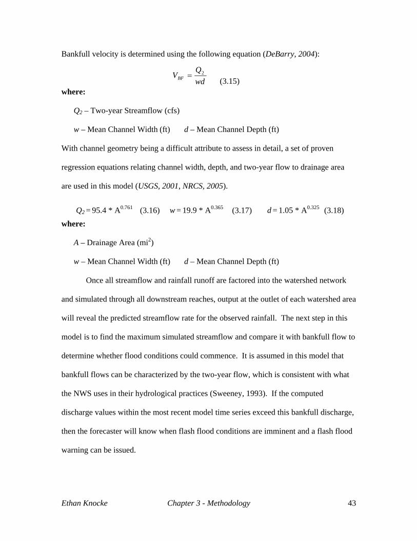
Bankfull velocity is determined using the following equation (DeBarry, 2004):

wdQ

VBF2=

(3.15)where:

Q2 – Two-year Streamflow (cfs)

w – Mean Channel Width (ft) d – Mean Channel Depth (ft)

With channel geometry being a difficult attribute to assess in detail, a set of proven

regression equations relating channel width, depth, and two-year flow to drainage area

are used in this model (USGS, 2001, NRCS, 2005).

(3.16) (3.17)


Q2 = 95.4 * A0.761 w = 19.9 * A0.365 d = 1.05 * A0.3255 (3.18)where:

A – Drainage Area (mi2)

w – Mean Channel Width (ft) d – Mean Channel Depth (ft)

Once all streamflow and rainfall runoff are factored into the watershed network

and simulated through all downstream reaches, output at the outlet of each watershed area

will reveal the predicted streamflow rate for the observed rainfall. The next step in this

model is to find the maximum simulated streamflow and compare it with bankfull flow to

determine whether flood conditions could commence. It is assumed in this model that

bankfull flows can be characterized by the two-year flow, which is consistent with what

the NWS uses in their hydrological practices (Sweeney, 1993). If the computed

discharge values within the most recent model time series exceed this bankfull discharge,

then the forecaster will know when flash flood conditions are imminent and a flash flood

warning can be issued.

If discharges within the series do not exceed bankfull, the model first gives a

flood threat level to describe how close water levels will get to flood stage and then

determines the amount of rainfall needed in a one and three hour period to ramp

streamflow levels up to flash flood levels. FFG rainfall depth categories were developed

to relate with simulated discharge differences between current peak flows and bankfull

flows using evenly distributed rainfall depths within the one and three hour time periods.

Rainfall depths from zero to 3.25 inches were evaluated at intervals of 0.25 inches by

dividing the rainfall depth into equal five minute periods throughout the one hour (depth /

12) and three hour (depth / 36) hypothetical rainfall events. These hypothetical storms

were then simulated using the basic hydrological modeling structure within this thesis

model for all three AMC conditions. Initial streamflow conditions were set to zero and

initial abstractions were nullified so that the only discharge increases within the output

hydrograph result from direct runoff contributions from the hypothetical rainfall

distribution. Each rainfall depth, duration, and AMC combination was simulated out six

hours from the beginning of the rainfall in order to obtain the entire evolution of the of

the rainfall-runoff process and determine the maximum discharge rate from the output

hydrograph that would be experienced within each watershed during the defined flash

flood duration.

With all model calculations computed, the GIS interface is then utilized to

symbolize each watershed in a variety of ways for visualization and hydrologic

interpretation purposes. The following characteristics are archived throughout the storm

event process and are available for mapping options:


• Total Rainfall – Accumulative storm total

• Excess Rainfall – Accumulative excess

• Saturation Rainfall – Additional rainfall required to satisfy initial abstractions

• Runoff CN – The computed storm event CN used within the FFG model process

• Peak Discharge – The current simulated peak discharge

• Flash Flood Risk – The current threat index, and previous flood duration

• One Hour FFG –Rainfall required in a one hour period to initiate flooding

• Three Hour FFG – Additional rainfall required in a three hour period

This GIS interface also has the capability to plot the following attributes for each

watershed:

• Storm Hydrograph – Simulated discharge for storm event at watershed outlet

• FFG – Evolution of predicted FFG thresholds through the course of a storm event

• Five Minute Rainfall – Observed Five Minute MAP distribution

• Total Rainfall – Accumulative rainfall distribution

A plot can be generated for any watershed within the study area by clicking within the

watershed area using one of the following mouse click options:

• Left Mouse – Storm Hydrograph

• Right Mouse – One Hour FFG

• Shift + Left Mouse – Five Minute Rainfall

• Shift + Right Mouse – Accumulative Rainfall Total


3.2 Model Implementation

This model operates in the ArcObjects environment of the ArcGIS 8.3 program

by repeating a series of functions to update the rainfall-runoff process and resulting storm

hydrograph evolution for every radar scan within the storm simulation. Functions access

and alter input variables from attribute tables, read rainfall text files to interpolate MAP

values for each radar scan, re-compute and store UH and storm hydrographs for each

watershed in .dbf tables, route runoff from headwater watersheds to the study area outlet

by tracking discharge evolution in two-dimensional arrays and tables, and update peak

discharge and FFG values. Tables needed for this model include (by name): Storm,

Wshds_Time, Wshds_Discharge, UH_5Min, Previous_Hydrograph, Storm_Hydrograph,

Simulated_Hydrograph, Hydrograph, and FFG. The continuous loop evolves in the

following schematic:

• Access MAP text files from NWS AMBER program for the duration of the storm

event and name each file in order starting at one

• Process through all MAP files to compute five minute rainfall depths for each

watershed and store them in the Storm table

• Access five-day rainfall total text file from NWS AMBER program to be used in

AMC classification and store them in the watershed attribute table

• Utilize the AMC value to adjust the normal watershed CN using the polynomial

CN adjustment equations and store the storm CN in the watershed attribute table

• Loop through rainfall depths for the number of scans involved in the storm

1. Store hydrograph from previous radar scan in a separate table (copy values

from Simulated_Hydrograph table into Previous_Hydrograph)


2. Read watershed area, length, slope, CN, and AMC from the watershed

attribute table and compute Tp and Qp for SCS UH ordinates generation

3. Utilize Tp and Qp ordinates table ratios to compute the 26 simulated UH

points for each watershed and store the time values in Wshds_Time and

discharge values in Wshds_Discharge

4. Use linear interpolation equations to interpolate between 26 known points at a

five minute time duration to form a simulated five minute UH and the series in

the UH_5min table

5. Use the SCS-CN equations to determine how much excess rainfall would

result for a given five minute rainfall depth (only applicable when all initial

abstractions are met)

6. Scale down the five minute storm UH to the actual amount of direct runoff

simulated and overwrite the UH_5min table with the simulated five minute

hydrograph

7. Offset the previous five minute hydrograph ahead one time step and then add

the current hydrograph onto the previous to form the updated storm

hydrograph and store this summation simultaneously in the

Storm_Hydrograph and Simulated_Hydrograph tables

8. If excess rainfall exists in any of the 35 watersheds, then perform the

Muskingum stream routing procedures for required watersheds, storing

subreach discharge inventories in arrays and output discharge values in the

Simulated_Hydrograph table


9. Store the first discharge value of the final simulation hydrograph for the

current five minute radar scan in the storm event hydrograph table

(Hydrograph) at the correct time slot within the storm evolution

10. Process through the current five minute simulation hydrograph to determine

the simulated peak discharge and compare that value with bankfull discharge

values to determine flash flood threat levels

11. Determine the difference between bankfull discharge and the current peak

discharge and assign this magnitude to a corresponding one and three hour

FFG (storing values in FFG tables)

• Symbolize and label the watershed layer within the GIS Interface with the

characteristic chosen by the user

Figure 8 provides a visual flowchart of this model process:

Figure 8 – FFG Model Flowchart


3.3 Model Improvements to FFG System

The use of embedded GIS in this FFG model creates a centralized process that

gathers required input data, computes parameters, simulates runoff potential, determines

the flood threat of a watershed, and displays FFG values for forecaster interpretation

within the same computer environment without the use of any external coupled model.

This model can give forecasters and hydrometeorologists a real-time inventory of rainfall,

direct runoff contributions, streamflow rates for gaged and ungaged watersheds, flash

flood threat, and resulting FFG. This model can also become a standard system that is

used across the country, and will work on any computer that has access to ArcGIS

software and extensions. Key reasons why the embedded GIS framework is

advantageous in this process include:

• Eliminating the need for coupling a hydrologic runoff simulation model with the

FFG system, everything is done within the same GIS program

• Most of the data required in this model scheme (watersheds, elevation,

hydrography, NLCD, HSG) are already developed in a GIS compatible format

• Having an embedded programming environment in ArcObjects to customize

ArcGIS to facilitate all formulas, computations, data manipulation, and output

display procedures of this FFG system

• The ability to analyze spatial watershed characteristics and compute required

parameters using the analysis tools available in ArcGIS

• The ability to store watershed geometry and the numerous lumped attributes for

these watersheds within the vector data structure


• Having a spatially oriented database structure that can be easily stored,

manipulated, and queried when results are computed

• The ability to access and handle very large spatial watershed databases; the

hydrograph table in particular because it contains simulated discharge values for

each watershed at five minute intervals for up to 20 hours

• Having a display environment available in ArcMap to display watershed

attributes, symbolize flood threat levels, and label watershed with output FFG

• The ability to query results interactively and plot hydrographs, FFG, and rainfall

by watershed to visualize when flood conditions may become imminent

• The flexibility in graphics user interface (GUI) development, which leads to the

development of user friendly programs

3.4 Model Assumptions

In order to model a complex flash flood guidance model in GIS that:

• is both flexible and effective,

• fits the scope of available data and hydrologic theory,

• requires small data storage and manageable computation,

• still provides good simulations of flood potential

there is a set of assumptions that have to be included in the modeling process to help

generalize the vast continuous earth into a suitable modeling environment. Assumptions

and generalizations that are included in this FFG include:

• 30 meter NED, NLCD, and SSURGO raster data provide accurate representations

of land surface and terrain characteristics


• Watershed attributes can be lumped to the small spatial scale of the watersheds

and still effectively represent the hydrologic composition of the region that they

encompass (the largest watershed area in this study area is 9.5 square miles)

• Rainfall accumulation can be accurately determined using MAP from the NWS

AMBER program at the radar time interval of four to six minutes

• AMC conditions can be broken down into dry, normal, and wet using the dormant

five-day rainfall intervals listed in Table 4

• AMC can be categorized using the five-day rainfall total developed by AMBER

• Antecedent streamflow conditions can be initialized for storm event simulation

using 15 - 30 minute observed USGS streamgage records

• The SCS-CN method and SCS-DUH procedure provide an accurate simulation of

the rainfall-runoff process for flash flood purposes

• A linear interpolation can be implemented between known time-discharge pairs of

the SCS-DUH at five minute intervals

• Streamflow routing downstream can be accounted for using the Muskingum

method

• Channel geometry can be determined using a set of developed regression

equations relating baseflow, two-year flow, width, and depth to drainage area

• The weighting factor (x) can be factored into the Muskingum formulas as a fixed

value of 0.25 because it represents the mean wedge coefficient or attenuation

factor

• Bankfull velocity can be directly related to the two-year flow of a stream segment


3.5 Data Sources and Development

There are many GIS layers involved in the model parameter development and

implementation of this FFG system. All provided layers were converted from the data

source coordinate system into an Albers projection because the Albers system preserves

area well within the United States. The following list describes each data type, the data

source, and its application in the model process.

• Watersheds – a basin shapefile provided by Paul Jendrowski of the NWS

Blacksburg Office (NWS, 2004). The watersheds were delineated for the

AMBER program and are at the spatial scale of flood analysis within the NWS

FFG system. This file is used to determine drainage area and is used as a

boundary for computing lumped watershed parameters needed in the model

(Figure 9).

• Streams/Rivers – a second shapefile provided by Paul Jendrowski, because it is

the stream file used by the AMBER program (NWS, 2004). The file follows the

National Hydrography Dataset (NHD) standards and contains many attributes

about the stream segments. This file is used for finding stream lengths and

determining overland travel distances to the nearest stream catchment (Figure 9).


Figure 9 – Map of Watershed and Stream Data Data Source: (NWS, 2004)

• Elevation – a 30 meter resolution grid that was downloaded from the USGS

seamless data server (USGS, 2004). The elevation data is a part of the National

Elevation Dataset (NED). A continuous elevation dataset is used to determine

terrain related characteristics such as land slope and runoff direction (Figure 10).


Figure 10 – Map of Elevation Data Data Source: (USGS, 2004)

• Land Cover – a 30 meter resolution grid that was also downloaded from the

USGS seamless data server (USGS, 2004). The land cover grid is a part of the

National Land Cover Dataset (NLCD). Land cover classes are used in

conjunction with the hydrologic soil group (HSG) to determine the runoff curve

number (CN) over the land area (Figure 11).


Figure 11 – Map of Land Cover Data Data Source: (USGS, 2004)

• Soil Type – grid data was developed during the implementation of a master’s

thesis by Brian McCormick (McCormick, 2003). The original data source was a

SSURGO polygon shapefile for the study area that was converted into a 30 meter

resolution grid to match the elevation and land cover grids. Soil type classes are

used to determine the HSG that the soil at a given location falls under and help to

determine CN (Figure 12).


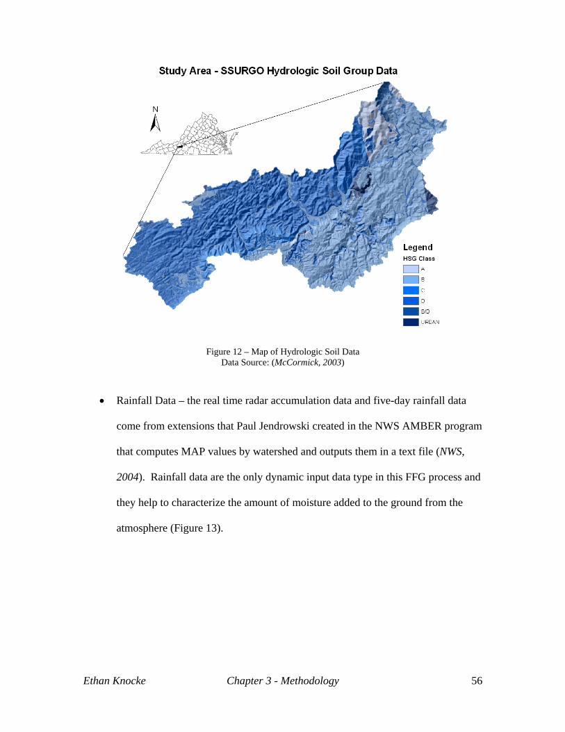
Figure 12 – Map of Hydrologic Soil Data Data Source: (McCormick, 2003)

• Rainfall Data – the real time radar accumulation data and five-day rainfall data

come from extensions that Paul Jendrowski created in the NWS AMBER program

that computes MAP values by watershed and outputs them in a text file (NWS,

2004). Rainfall data are the only dynamic input data type in this FFG process and

they help to characterize the amount of moisture added to the ground from the

atmosphere (Figure 13).


Figure 13 – Sample Rainfall Input Text File Generated by AMBER (Depth in last column) Data Source: (NWS, 2004)

• Streamgage Data – this data was developed by the USGS and distributed by

Shaun Wicklein of the Virginia Water Science Center. The data file contains 15 –

30 minute continuous observed unit stream discharge from July 2003 to January

2005 and is used to initialize streamflow rates for storm events and to validate

model simulations (Figure 14).


Figure 14 – Shawsville USGS Streamgage File (Streamflow in fourth column) Data Source: (USGS, 2005)

3.6 Storm Events

In order to test the accuracy and effectiveness of the hydrologic modeling

techniques and embedded GIS functionalities used in this FFG system, a set of ten

historical storm events were selected to serve as case flood events. Storm event criteria

included the relative flash flood threat to the study area, the type of weather event that the

storm represents, the movement of the storm, the orientation of the storm in relation to

the stream network, and the magnitude of the peak discharge observed at the Shawsville

gage. These criteria were further limited to the previous two years because this model

utilizes NWS AMBER rainfall data, which is only archived back to January 2003. Storm

events were selected by looking at the following four weather and hydrology sources:


• 1. National Climatic Data Center Storm Event Database (NCDC, 2005)

• 2. NWS Blacksburg Preliminary Climate Data (NWS, 2005)

• 3. USGS Surface Water Peak Streamflow Archive for Shawsville (USGS, 2005)

• 4. USGS 15 - 30 Minute Streamflow Dataset for Shawsville (USGS, 2005)

Table 7 lists the storm events utilized in this research in chronological order, with rainfall

and discharge ranges characterizing the time interval of simulation:

Source Date Type Movement, Orientation

5 Day Rainfall

Storm Rainfall

Peak Discharge

Flood Threat

2 7/1/2003 Low NE, ⁄⁄ 0.06-2.24 0.35-1.05 473 N 1 7/6/2003 Convection E, ⁄⁄ 0.68-1.95 0.25-1.85 2530 Y 1 9/18/2003 Tropical NW, ┴ 0.01-0.14 0.94-3.77 3220 Y 1 11/19/2003 Front E, ⁄⁄ 0.07-0.19 0.63-1.31 2050 N 4 4/13/2004 Low NE, ⁄⁄ 0.35-0.68 0.22-0.51 880 N 2 9/8/2004 Tropical NE, ⁄⁄ 0.01-0.55 0.42-2.86 3480 Y 2 9/17/2004 Tropical NE, ⁄⁄ 0.00 0.3-1.22 916 N 3 9/28/2004 Tropical N, ┴ 0.00-0.02 1.78-4.7 7390 Y 4 11/24/2004 Low E, ⁄⁄ 0.00-0.38 0.36-0.85 1620 N 1 1/14/2005 Front E, ⁄⁄ 0.00-0.56 0.7-1.19 1730 N

Table 7 – Case Storm Events

3.7 Discussion of Model Parameters

The four processes involved in this FFG model (SCS-CN, SCS DUH,

Muskingum, and FFG) have a diverse set of parameters in their formulas that help to

simulate the rainfall-runoff process and predict bankfull flow development. These

parameters include:

• Direct Runoff (Q) – represents the amount of liquid water from rainfall that

contributes to the watershed stream network as discharge. This value is computed

using the SCS-CN method equation (3.1). Direct runoff will only commence

when rainfall totals have matched or exceeded the initial abstraction levels of the


watershed. In the SCS DUH formulation, it is assumed that there is one inch of

direct runoff in the rainfall excess duration.

• Rainfall (P) – quantifies the amount of rainfall that has fallen on the surface as a

lumped MAP for the watershed catchment. This value is used to reveal the

amount of liquid water that is added that can potentially be converted into runoff

into the stream network after all abstractions have been removed. MAP is

computed within the NWS AMBER program.

• Antecedent Moisture Condition (AMC) – an adjustment factor on CN used to

account for the amount of moisture present within the ground at the beginning of

a storm event. In literature the AMC category is assumed to be broken down

based on the dormant five-day accumulative rainfall total, which is also computed

using the NWS AMBER program.

• Initial Abstraction (Ia) – characterizes the amount of rainfall that can be stored in

surface depressions or through interception. This parameter is computed using

the SCS-CN method equation (3.3).

• Storage Retention (S) – helps to categorize the maximum amount of rainfall that

can be directly stored in the ground through abstractions. This value is

characterized based on the land use, land cover, soil type, hydrologic condition,

and AMC and is related to the CN of a watershed using the SCS-CN method

equation (3.2)

• Curve Number (CN) – categorizes the runoff potential that exists for a watershed

region on a scale from zero to 100. This number is determined on a cell by cell

basis within the NLCD and HSG grids using a curve number table that relates


land cover and soil type, and is then altered using equations (3.5) and (3.6) based

on the AMC levels (dry, average, and wet)

• Basin Lag Time (Tl) – quantifies the time lag between the middle of the rainfall

excess period and the peak discharge at the outlet of a watershed. It is computed

using the SCS equation (3.7)

• Length to divide (L) – measures the distance along the main channel of a

watershed up to the furthest upstream divide. This distance helps to characterize

the maximum length that rain water will have to travel as direct runoff down the

outlet. This parameter is computed using the “flowlength” function in the Spatial

Analyst environment of ArcGIS.

• Average Land Slope (Y) – describes the mean slope of land within the watershed

where overland flow takes place. The slope of this component of a watershed

determines how quickly direct runoff will flow over the surface down to the main

channel. To determine this function, a slope grid was calculated using the “slope”

function on the elevation grid in spatial analyst. Then, the “zonalmean” function

was used to determine the mean slope by watershed.

• Duration of Rainfall Excess (ΔD) – quantifies the time lapse between initiation

and termination of rainfall excess within the watershed. The duration of rainfall

excess reveals how much time there is for potential direct runoff contribution into

the main channel network. This is defined to be five minutes in this model

because this will match the approximate five minute time interval of radar input.


• Time to peak discharge (Tp) – describes the time lapse between runoff initiation

in the streams and rivers and the peak discharge simulated at the outlet using the

SCS DUH equation (3.8).

• Peak Discharge (Qp) – defines the maximum discharge that will occur at the

outlet at the peak discharge time. This peak discharge generated from simulated

direct runoff in the water is calculated using the SCS DUH equation (3.9).

• Drainage Area (A) – measures the land area of the catchment region that a given

watershed covers. This area is delineated based on topographic divides and other

boundaries that alter the directionality of runoff flow. Drainage area came as an

attribute within the watershed shapefile provided by the NWS.

• Outflow (O) – represents an initial and final outflow parameter used within the

Muskingum method to route runoff contributions to streamflow through a

watershed channel reach. These parameters simulate the outflow discharge at the

outlet of a watershed at the beginning and end of a routing time step. The values

are computed and used in the Muskingum equation (3.10).

• Inflow (I) – represents an initial and final inflow parameter used in the

Muskingum method to quantify discharge contributions into a watershed

catchment from upstream. The values are computed and used in the Muskingum

equation (3.10).

• Coefficients (C) – are equation component coefficients used to characterize the

hydrologic offsets required to accurately depict routing of runoff water through a

stream reach in the Muskingum method. The three coefficients are computed

using equations (3.11 – 3.13).


• Travel Time Constant (K) – is used within Muskingum coefficient equations to

describe the time it takes for a bankfull velocity flow rate to travel through the

stream reach of a watershed. This parameter is computed using equation (3.14).

• Weighting Factor (x) – is used within Muskingum coefficient equations to

characterize the storage and attenuation capabilities of a stream reach. These

values range between zero and 0.5 and in this model the factor is assumed to be

an average value of 0.25.

• Routing Time Step (Δt) – is used within the Muskingum coefficient equations to

tag the time step associated with the routing procedure. This value is assumed to

be five minutes, in order to match the time interval associated with the SCS-CN

and SCS DUH methods.

• Reach Length (R) – represents the length of the main concentrated flow channel

of a watershed. This section of the watershed accounts for the area where routing

is influenced the most in the process of transitioning runoff water through a

catchment zone. The length was computed by calculating the stream distance

within the streams shapefile.

• Bankfull Velocity (VBF) – represents the streamflow rate that would be observed

if the stage height of a stream or river was at the bankfull level. This velocity

quantifies the speed to which water would travel through the channel network at

the bankfull stage. This parameter is determined for each watershed based on

watershed geometry and flow characteristics using the equation (3.15).

• Two-Year Streamflow (Q2) – quantifies the estimated discharge within the

channel in a two-year return period. In this FFG model, Q2 is assumed to be the


flood stage discharge for each watershed. The flow rate is determined using the

regression equation (3.16)

• Mean Channel Width (w) – characterizes the mean width of the concentrated

channel of a watershed catchment. The value is determined in this model using

the regression equation (3.17)

• Mean Channel Depth (d) – characterizes the mean depth of the concentrated

channel of a watershed. This works in conjunction with the mean width to

provide a generalized geometric representation of the stream channel network.

The value is determined using the regression equation (3.18)

3.8 Model Sensitivity

With all of the parameters, equations, regressions, assumptions, and limitations

involved in this FFG modeling sequence, there is a set of attributes to the model that are

tested within this research to reveal their sensitivity and influence on model results. The

following sensitivity analyses were performed:

- Impacts of error in DEM grid on watershed delineation, overland and streamflow

dynamics, and lumped parameter estimation

- Impacts of AMC on moisture initialization and direct runoff generation

The purpose of the DEM sensitivity analysis is to determine the impact that error

in the National Elevation Dataset (NED) has on watershed and hydrology parameters.

These parameters include the watershed area, mean slope, length to divide, mean CN, UH

time to peak discharge, and UH peak discharge. This will help to characterize

uncertainties that may exist in UH generation and FFG development as a result of terrain


and watershed induced error in these input parameters. It should be noted that stream

geometry, watershed shape, and lumped parameters in the FFG model developed from

this research will not be altered from their initial state based on the results of this analysis

because it is important to utilize the same input watersheds and streams that the NWS

uses in their lumped AMBER rainfall software for rainfall-runoff consistency.

Metadata for the USGS NED states that there is a RMSE in modeled elevation of

up to seven meters at a given grid cell location. This error can significantly impact the

surface runoff dynamics of a region, which would alter watershed shapes and the lumped

characteristics of these watersheds. To determine the magnitude of these acknowledged

vertical errors, five spatially autocorrelated random error grids were used in this

assessment to alter the source NED data, delineate watersheds and streams, re-compute

terrain related parameters, compare values with current parameter values used in my FFG

model, and determine how this error can effect UH shapes. It is assumed for this analysis

that error should not exceed one contour interval, which in this region is 20 feet

(approximately 6 meters).

The random grid generator function in spatial analyst (rand()) was used to create

the uniformly distributed error values for each pixel within the study area. The focal

mean smoothing function (focalmean()) was performed using a five by five mean matrix

to smooth error values down to the desired +/- six meter range and achieve the necessary

spatial autocorrelation to effectively simulate terrain error. Figure 15 shows the error

generation process:


+

Figure 15 – Elevation Error Grid Generation

This created seven scenarios (model, NED, and five error grids) that were used to

determine the impact of vertical error on input parameters. The model scenario use the

watershed and stream geometry provided by the NWS, the NED scenario follows

geometry and parameters computed using the source USGS NED, and the five error grids

each follow geometry and parameters computed using each perturbed NED grid.

The purpose of the AMC sensitivity analysis is to determine the impact that

categorized CN adjustments have on lumped CN estimation, initial abstraction

computation, and direct runoff generation. CN based models and the criteria and

assumptions that come with them can be effective in simulating the rainfall-runoff

process, but at this point CN and AMC theories are not an exact science. They do not

function well during the winter months when snowmelt and frozen soils can impact

infiltration and AMC categories, the assumption that five-day rainfall classes can

categorize AMC may not always work during times of drought or excessive rainfall, and

holding AMC and CN constant throughout a storm event is a basic attempt at simulating

the hydrologic response of the environment.

Storm events will be simulated utilizing the AMC criteria provided in the

literature (Table 4), simulated by holding CN at a constant AMC II state below the AMC


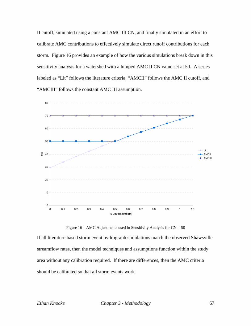
II cutoff, simulated using a constant AMC III CN, and finally simulated in an effort to

calibrate AMC contributions to effectively simulate direct runoff contributions for each

storm. Figure 16 provides an example of how the various simulations break down in this

sensitivity analysis for a watershed with a lumped AMC II CN value set at 50. A series

labeled as “Lit” follows the literature criteria, “AMCII” follows the AMC II cutoff, and

“AMCIII” follows the constant AMC III assumption.

0

10

20

30

40

50

60

70

80

0 0.1 0.2 0.3 0.4 0.5 0.6 0.7 0.8 0.9 1 1.1

5 Day Rainfall (in)

CN

LitAMCIIAMCIII

Figure 16 – AMC Adjustments used in Sensitivity Analysis for CN = 50

If all literature based storm event hydrograph simulations match the observed Shawsville

streamflow rates, then the model techniques and assumptions function within the study

area without any calibration required. If there are differences, then the AMC criteria

should be calibrated so that all storm events work.


4.0 Results

4.1 Elevation Sensitivity

There were differences found between stream and watershed delineations in the

seven scenarios described in section 3.8. After visualizing these differences, it was found

that headwater tributaries and small stream segments within higher elevations do not

deviate due to NED error as much as downstream segments and branch confluences that

have wider channel geometries. Watershed deviations also exhibited these same

characteristics, with the greatest deviation occurring at the eastern branch confluence and

the outlet of this study area. Differences in boundaries also exist along the western

border of the South Fork region where smaller ridges form the watershed boundaries.

Figure 17 and 18 show the differences that exist within the study area:

Figure 17 – Watershed Delineations

Ethan Knocke Chapter 4 – Results 68

Figure 18 – Stream Delineations

Terrain characteristics varied between the scenarios in different ways. Area

varied most within the watersheds where boundaries varied the most near branch

confluences (IDs 6, 7, 10, 12, 14, 16, and 17). Mean slope and CN did not vary as much

between the seven scenarios, most likely because small variations in watershed

boundaries of this size get nullified by the large number of 30 meter grid cells involved in

the lumped parameter estimation. Length computations varied the most because this is

the only parameter that is computed in a continuous distributed manner. With random

perturbations in terrain shape, flow direction and accumulation can be altered

significantly on the small scale. The most substantial differences occurred within IDs 6,

7, 9, 10, 14, 16, and 17. These results reveal that elevation error on the local scale will

have the most impact within the lumped SCS UH modeling environment on drainage area

and flow length. Tp and Qp coefficients varied on the same pattern as these two

parameters.


Tp and Qp coefficients were then used to develop UH curves for each watershed

using values computed within the seven scenarios and the SCS UH ordinates tables. To

help visualize the effects that elevation error can have on SCS UH generation, UH plots

were developed for three watersheds. Watershed 0 (Figure 19) was graphed to reveal the

limited impact the elevation error has on upstream headwater watersheds, watershed 10

(Figure 20) was graphed to show error impacts within wider downstream segments and

confluence regions, and watershed 25 (Figure 21) was graphed to characterize the

impacts of small low elevation terrain divides and watershed boundaries like the ones

seen in the western border of this study area. Table 8 contains parameter ranges

computed between the seven scenarios and percent differences for these three

watersheds:

ID Area (mi2) Slope (%) CN Length (ft) Tp (hrs) Qp (cfs) 0 6.08-6.10

0.21% 25.09-25.14

0.20% 54.55-55.06

0.93% 33,760-34,455

2.04% 2.13-2.17

1.86% 1,352-1,381

2.12% 10 1.26-1.49

15.16% 28.36-29.71

4.65% 70.24-70.30

0.08% 12,013-14,297

17.36% 0.61-0.69 13.95%

905-1,018 11.75%

25 3.50-3.76 7.16%

15.32-15.85 3.40%

66.17-72.45 9.06%

17,109-21,845 24.32%

1.01-1.44 35.10%

1,253-1,681 29.18%

Table 8 – Elevation Error Sensitivity Sample Results

Differences that may exist between the model results and the other six scenarios due to

the fact that this scenario utilizes watershed and stream geometry provided by the NWS,

while the other six geometries were derived using hydrology tools on the source NED

and error grids.


0

200

400

600

800

1000

1200

1400

0 1 2 3 4 5 6 7 8 9 10 11

Time (hr)

Dis

char

ge (c

fs)

ModelNEDError 1Error 2Error 3Error 4Error 5

Figure 19 – UH Curves (Upstream Watershed)

0

200

400

600

800

1000

1200

0 0.25 0.5 0.75 1 1.25 1.5 1.75 2 2.25 2.5 2.75 3 3.25 3.5

Time (hr)

Dis

char

ge (c

fs)


Figure 20 – UH Curves (Confluence Watershed)


0

200

400

600

800

1000

1200

1400

1600

1800

0 1 2 3 4 5 6 7 8

Time (hr)

Dis

char

ge (c

fs)


Figure 21 – UH Curves (Weak Boundary Watershed)

In summary, geometry results reveal that elevation error does not lead to

significant alteration of watershed boundaries and stream channels within higher

elevation upstream headwater regions with crisp ridge divides and narrow, well-defined

channel geometries. However, as you travel downstream to wider channel reaches and

regions around forks and branch confluences, elevation error can significantly alter

drainage areas, boundary locations, and stream shapes. In this study area, sections of the

stream reaches within watersheds 6, 12, and 14 were simulated 250 to 500 meters apart.

Watershed areas were altered the most by elevation error in complex confluence regions

(e.g. IDs 6, 7, 12, 14, 16, 21) and within valley drainage areas with small fuzzy terrain

divides and boundaries (e.g. IDs 9, 25, 26, 29, 31, 32, 33).

Terrain parameters within the lumped SCS-UH method are impacted in a variety

of ways; with mean slope and CN not being perturbed as much by error, and area and


flow length being altered more due to their heavier sensitivity to watershed shape and

flow dynamics. Again, these impacts were seen most within lower elevation downstream

reaches near the outlet of the South Fork and along watershed regions with weaker ridges

for drainage divides such as the ones found in the western side of this study area.

Tp and Qp were altered among the simulations in a given watershed based on the

impact that elevation error had on the terrain parameters involved in SCS UH equations.

SCS UH curves varied significantly within the downstream watersheds and the western

watersheds, where elevation perturbations influenced Tp and Qp the most. Discharge

values immediately around Tp and to the right of Tp during recession seem to vary the

most in these situations. This is because varying parameter results impacted the assigned

time of concentration for a watershed, which altered the timing of Tp and corresponding

magnitude of Qp. Overall, these sample graphs help to show that elevation error can lead

to differences in UH shape, which can accumulate over time within a storm simulation to

create dramatic differences in storm hydrograph evolution. Although in this five minute

FFG model, differences in UH shape may not be as significant for smaller storm events

with minor runoff contributions because the very small direct runoff depths associated

with this short of a time span will dramatically reduce the discharge values throughout

the curve.

This sensitivity analysis of elevation error illustrates the minimal impact that

NED error can have on higher elevation headwater regions and the importance of

accounting for elevation error in hydrologic parameters and model simulation within

wider downstream reaches and watershed areas with smaller divides. In order to clear

uncertainties in elevation error on UH shape, hydrologists should visualize observed gage


hydrographs to determine whether computed Tp values are too quick or are delayed and

resulting Qp values are overshooting the peak or are too low. Confidence intervals in

drainage area, flow lengths, and Tp and Qp UH parameters should be included within

hydrological analyses using the range between maximum and minimum terrain parameter

values within NED error scenarios. This way, meteorologists and hydrologists will

understand impacts that elevation error may have on their current river and stream

forecasts and resulting FFG.

4.2 Antecedent Moisture Condition (AMC) Sensitivity

Simulation of the ten storm events was first performed using the standard SCS-

CN procedures and AMC adjustments that are provided in the hydrology literature. Five-

day rainfall is computed as a single accumulative MAP by watershed using the AMBER

program. Then the computed mean CN is adjusted to account for soil moisture using the

default dormant five-day rainfall total CN adjustments (Table 4) and the polynomial

equations (Table 5) developed from these cutoffs to relate accumulative rainfall to a

representative runoff CN.

There were mixed results in using this literature based method of runoff

computation and soil moisture content, depending on the time of year that the storm event

occurred, the time interval between the previous rainfall and the storm, the amount of

rainfall and resulting direct runoff associated with the event, and the type of storm event.

Variation from the observed USGS streamflow record at the study area outlet in

Shawsville was found to be heavily influenced by whether the initial abstractions


determined from the adjusted CN value could be met by the AMBER MAP rainfall total,

and if so how far into the storm event direct runoff commenced.

With this study area being a heavily forested region, lumped CN values in normal

conditions (AMC II) were in the range of 45 to 72 with a mean of 65. Adjusting this

normal CN down to dry conditions (AMC I) causes many of the watersheds to have very

low CN values, under which the SCS-CN method would require very large initial

abstractions be met before direct runoff can commence. Sole use of the five-day rainfall

less than 0.5 inches criteria for CN adjustment to AMC I caused many of these ten storm

events to fall within this AMC I category, which led to very low runoff production

because of the large initial abstractions. From Table 7, seven of the ten storm events

have the majority of the 35 study area watersheds attaining a five-day rainfall total that is

at or well below the 0.5 inch cutoff for AMC II, meaning that the entire area will default

to CN values less than the normal AMC II condition. This caused many of the storms

totals to never exceed the predicted Ia, which obviously does not function well

considering that all ten of these storms met initial abstraction levels and initiated direct

runoff contribution into the streams. Table 9 shows results of how the ten storm events

simulated using the literature methodology:

Storm AMC CN Ia Rainfall Watersheds with Pe = 0

Pe Simulated Peak

Observed Peak

7/1/2003 I - III 32-85 0.18-4.16 0.35-1.05 18 0.0003-0.13 216 473 7/6/2003 II - III 60-85 0.32-1.32 0.25-1.85 14 0.00007-0.56 3870 2530 9/18/2003 I 27-56 1.56-5.35 0.94-3.77 29 0.0008-0.13 55 3220

11/19/2003 I 33-55 1.68-4.02 0.63-1.31 35 0.00 85 2050 4/13/2004 I - II 42-75 0.65-2.75 0.22-0.54 35 0.00 300 880 9/8/2004 I - II 35-62 1.23-3.82 0.42-2.84 31 0.005-0.19 1931 3480 9/17/2004 I 25-50 2.04-5.82 0.3-1.22 35 0.00 50 916 9/28/2004 I 25-50 1.96-5.96 1.78-4.7 6 0.0002-0.55 151 7390

11/24/2004 I 29-55 1.59-4.84 0.35-0.84 35 0.00 350 1620 1/14/2005 I - II 29-57 1.49-4.84 0.7-1.19 35 0.00 99 1730

Table 9 – Literature Simulation Results for Ten Case Storm Events


With the limited success of utilizing the AMC CN adjustments provided in the

literature to simulate these ten storm events, the other two CN adjustment factors were

implemented for storm simulation (AMCII and AMCIII described and graphed in section

3.5). The following few pages reveal the results of each simulation and how sensitive the

rainfall-runoff process is to soil moisture adjustments. Figures 22 through 31 provide

plots of hydrographs of AMC simulations that initiated direct runoff for each case storm.

0

50

100

150

200

250

300

350

400

450

500

550

600

650

700

0 60 120 180 240 300 360 420 480 540 600 660 720 780 840 900 960 1020 1080 1140 1200

Time (Min)

Dis

char

ge (c

fs)

GageLitAMCIIAMCIII

Figure 22 – Hydrographs for July 1, 2003 Storm (1600 – 1200 UTC)

July 1, 2003 Storm

The first storm was difficult to simulate due to the extended duration that low

pressure rainfall contributed to direct runoff. There were two brief periods of rainfall that

occurred roughly 12 hours apart, followed by an extended period of light rainfall. Due to

the limitations in ArcGIS 8.3, simulation could only be carried out to account for the two

initial bursts. Therefore, results from this storm may not necessarily represent the correct

accuracy of the models ability to simulate this event. The majority of this rainfall (0.6 to


one inch) dropped in the eastern watersheds, where AMC rainfall was lower. According

to the literature, CN values needed to be very low (30 – 50), requiring more rainfall than

the observed amount to achieve runoff. Minimal excess rainfall amounts in these

simulations were confined to watersheds around the outlet, and only raised discharge

within the AMCIII simulation. Error in simulation of this storm event can be referenced

to the inability to simulate the entire storm event due to limitations in memory allocation

in ArcGIS 8.3, the subjectivity of CN classification, and incorrect AMC adjustments.

0

500

1000

1500

2000

2500

3000

3500

4000

4500

5000

5500

6000

0 30 60 90 120 150 180 210 240 270 300 330 360 390 420 450 480 510 540

Time (Min)

Dis

char

ge (c

fs)

GageLitAMCIIAMCIII

Figure 23 – Hydrographs for July 6, 2003 Storm (1500 – 0000 UTC)

July 6, 2003 Storm

This storm event was simulated best by this FFG model; with direct runoff

initiation occurring at the correct time and a slight offset of time of concentration and

resulting peak discharge magnitude. This storm event began with ample soil moisture

from previous rainfall (0.6 – 1.9 inches), making storm CN values and runoff potential


very high. This was a high intensity, short duration storm event, as some of the

watersheds received the majority of the rainfall from this event in less than an hour.

Heaviest rainfall totals and resulting direct runoff were at or immediately around the

outlet watershed. Early rise in the simulated hydrograph curves mean that literature

based UH Tp computations can be early in some storm events. Offsets in time of

concentration can be caused by errors in terrain, false classification of required CN, and

inaccuracy in CN adjustments based on AMC criteria. Having a lower Tp in the UH

formation causes Qp to be higher, which could be the reason for overshooting simulated

peak discharge.

0

500

1000

1500

2000

2500

3000

3500

4000

4500

5000

5500

6000

6500

7000

7500

8000

0 30 60 90 120 150 180 210 240 270 300 330 360 390 420 450 480 510 540 570 600 630 660 690 720 750 780 810

Time (Min)

Dis

char

ge (c

fs)

GageLitAMCIIAMCIII

Figure 24 – Hydrographs for September 18, 2003 Storm (1600 – 0600 UTC)

September 18, 2003 Storm

This storm was the first of four tropical events simulated in this research,

consisting of moderate rainfall that occurred for nearly ten hours. The event was difficult


to simulate due to the low five-day rainfall total that existed before it (0.01 – 0.14

inches). This caused initial abstractions to be so high that it took the majority of the

extreme rainfall from this event for the FFG model to recognize direct runoff using the

literature methodology. Rainfall amounts of two to three inches were heaviest to the

northeast of the outlet watershed, with direct runoff contributions within the AMCII and

AMCIII simulations primarily around the outlet. The AMCII simulation did initialize a

discharge increase at the right time, but direct runoff contribution from rainfall after this

time using the runoff potential associated with these sensitivity criteria was not enough

for the model to simulate a peak that matched reality. The AMCIII simulation also began

a discharge rise at the same time as the gage records, but discharge levels rose much

quicker and to a higher peak. Close proximity to the outlet; coupled with a high CN, low

time of concentration, and consistent direct runoff contribution are the primary reasons

for this offset in hydrography shape.

0100200300400500600700800900

1000110012001300140015001600170018001900200021002200

0 60 120 180 240 300 360 420 480 540 600 660 720 780 840 900 960 1020

Time (Min)

Dis

char

ge (c

fs)

GageAMCIII

Figure 25 – Hydrographs for November 19, 2003 Storm (0600 – 0000 UTC)


November 19, 2003 Storm

This ten hour event contained predominantly low intensity rainfall rates across the

entire study area with a brief period of moderate rainfall near the end at the time of the

frontal passage. Like the September 18th event, this was an isolated storm with rainfall

totals in the days leading up to this event between 0.07 and 0.19 inches. Initial

abstractions were met in all of the simulations within the previous event due to the

extraordinary amount of precipitation associated with the tropical system. However in

this event, lower rainfall totals of 0.5 – 1.3 inches were only able to counterbalance

assumed initial abstractions within the AMCIII criteria. Hydrograph simulation using

these criteria did contain a discharge rise at the same time and general rate as the gage

record, but the model simulation peaked out at an earlier time with lower discharge.

Upon comparison between the time that initial abstractions were met and when the

heaviest rainfall fell near the end of the event, it was found that direct runoff contribution

in the FFG model did not commence until this late time. Therefore, excess runoff depths

according to the model were very low, peaking out at only 0.1 inches. Extremely low,

evenly distributed simulated direct runoff at the end of the event is most likely to blame

for the lower peak discharge level simulated in this case.


0

50

100

150

200

250

300

350

400

450

500

550

600

650

700

0 60 120 180 240 300 360 420 480 540 600 660 720 780 840 900 960 1020

Time (Min)

Dis

char

ge (c

fs)

Gage

Figure 26 – Hydrographs for April 13, 2004 Storm (0600 – 0000 UTC)

April 13, 2004

The graph for this storm only contains the observed gage hydrograph because

initial abstractions were never met within all three of the AMC sensitivity analyses.

Therefore according to the criteria and assumptions involved in this FFG model and

AMC sensitivity assessments, direct runoff never occurred during this event.

Accumulative rainfall in the five days leading up to this storm event was between 0.3 and

0.8 inches, making runoff potential for watersheds at or below their normal AMC II state.

However, this was an event with a prolonged low rainfall rate that generated modest

rainfall totals between 0.25 and 0.5 inches over a six hour period. Not even setting runoff

CN values at their highest possible value within the AMCIII simulation could create low

enough initial abstractions for this rainfall to counterbalance. This storm event helps to

reveal that the SCS-CN method does not function correctly for isolated storm events that

accumulate minimal rainfall depths. Observed runoff patterns at the Shawsville gage for


this storm event required CN values to be higher than the range used in these dormant

AMC CN adjustments for the SCS CN and UH procedures to correctly simulate the

rainfall-runoff process and hydrograph volume.

0

500

1000

1500

2000

2500

3000

3500

4000

4500

0 60 120 180 240 300 360 420 480 540 600 660 720 780 840 900 960 1020 1080 1140 1200

Time (Min)

Dis

char

ge (c

fs)

GageLitAMCIIAMCIII



This was the first of three tropical events in September of 2004, with a consistent

light to moderate rainfall for 18 hours. Antecedent rainfall was between 0.01 and 0.5,

making AMC conditions at or below normal. Heaviest rainfall totals exceeding two

inches were found in the higher elevation eastern regions of this study area, with

significant direct runoff of 0.25 to 0.5 inches simulated along the eastern border

watersheds. Discharge contributions in the literature and AMCII state initiated much

later in the storm event and did not reach the correct peak, while AMCIII CN conditions

matched closer in timing with the Shawsville record. Again, the rising side of the

simulated hydrograph seems to increase quicker and slightly earlier, which could be


referenced to the improper use of SCS Tp equation parameters due to elevation or CN

error. Adjusting time of concentration to a longer duration and unit hydrograph shape to

the right can fix this mismatch.

0

50

100

150

200

250

300

350

400

450

500

550

600

650

700

750

800

850

900

950

1000

0 60 120 180 240 300 360 420 480 540 600 660 720 780 840 900 960 1020

Time (Min)

Dis

char

ge (c

fs)

GageAMCIII



This second tropical event in the series was also simulated quite well in

comparison to gage records. It also brought a prolonged light to moderate rainfall in the

eastern regions of this study area. Rainfall depths were on the order of 0.75 to one inch

in this event however, so simulated direct runoff was very low in the FFG model. There

was no observed rainfall in the five-days before this tropical event, so AMC CN

adjustments set mean CN values at their minimum. Direct runoff only initiated when

runoff potential was maximized within the AMCIII sensitivity analysis. The same issue

came up in this tropical event as in the previous, direct runoff initiated at the correct time


but the simulated discharge increased more rapidly. However in this storm event the

early rise peaked very close to the correct value and did not lead to a discharge overshoot.

A slight adjustment in runoff CN and time of concentration can correct this error.

0

2000

4000

6000

8000

10000

12000

14000

16000

18000

20000

22000

24000

26000

28000

30000

32000

34000

0 60 120 180 240 300 360 420 480 540 600 660 720 780 840 900

Time (Min)

Dis

char

ge (c

fs)

GageLitAMCIIAMCIII



The third tropical system out of this series was different from the other two

because even though there was also a prolonged duration to the event, there were three

brief periods of intense rainfall. The event brought the most rainfall out of the ten events

across the entire study area, with extreme rainfall amounts as high as 4.5 inches and high

amounts of direct runoff exceeding one inch over the majority of the region. The five-

day AMC was again initiated to be at zero, making direct runoff initiation in the literature

method unable to convert much of this extraordinary rainfall into direct runoff. However,

the cost of bringing CN adjustments up to the AMCII and AMCIII caused hydrograph

initiation to occur at the correct time, but discharge rates to rise much quicker than the


gradual ascent of the observed hydrograph. This rapid rise leads to a substantial

overestimation of the peak discharge by two to four times the observed value. This

extraordinary precipitation event shows that CN adjustment between AMC I, AMCII, and

AMCIII is not always effective enough in determining the correct runoff CN to

implement. Adjustment to AMCII alone for this event created a runoff CN that

converted far too much rainfall into runoff. Computing a study area wide observed CN

from the observed gage hydrograph for extraordinary tropical events can help to

determine the correct CN to utilize within extreme runoff events.

0

500

1000

1500

2000

2500

3000

3500

0 60 120 180 240 300 360 420 480 540 600 660 720 780 840 900 960 1020 1080 1140

Time (Min)

Dis

char

ge (c

fs)

GageAMCIII

Figure 30 – Hydrographs for November 24, 2004 Storm (1000 – 0600 UTC)

November 24, 2004 Storm

Like the July 6th storm event, the rainfall pattern of this case was brief, intense,

and located around the outlet. However this was an isolated storm event where AMC

conditions were dry, so discharge simulation only occurred within the AMCIII analysis.

Direct runoff in this simulation began at the same time as this brief burst of rainfall,


which is why discharge rapidly rose to the peak. This simulation also overshot the

observed peak because extreme runoff CN values were needed from the AMCIII

adjustment in order for discharge to be initiated.

0100200300400500600700800900

1000110012001300140015001600170018001900200021002200

0 30 60 90 120 150 180 210 240 270 300 330 360 390 420 450 480 510 540 570 600 630 660 690 720

Time (Min)

Dis

char

ge (c

fs)

GageAMCIII

Figure 31 – Hydrographs for January 14, 2005 Storm (1000 – 0300 UTC)

January 14, 2005 Storm

The final case in this analysis was also a storm with little to no AMC, causing CN

values to be extremely low and runoff response only to occur within the maximized

AMCIII conditions. An even distribution of 0.75 to one inch of rain fell in a moderate

rate leading to a similar distribution of direct runoff across the entire study area. One

difference with utilizing the AMCIII criteria in this storm is that direct runoff initiation

was late in this event and again simulated an extremely rapid discharge rise.

Overall, the analysis of these ten storm events shows that simple implementation

of the dormant AMC CN adjustment classifications can be ineffective in creating the

optimal runoff CN characteristics for storm events. Extremely dry weather patterns


before a storm event are not simulated well with these adjustments, marginal rainfall

events are not accurately simulated by the AMC I – III CN values, and overestimation of

direct runoff can occur within extraordinary rainfall events. Table 10 summarizes

characteristics of the closest curve out of the three simulations for each event:

Storm Option Mean CN

Gage Peak

Gage Time

Model Peak

Model Time

ΔT (hr)

ΔQ (cfs)

Q % Diff

Cross Correlation

7/1/2003 AMCIII 80 473 0230 728 1130 9 255 42.5 0.157 7/6/2003 Lit 76 2,530 2230 3,870 2200 -0.5 1,340 41.8 0.945

9/18/2003 AMCII 64 3,220 0500 2,324 0230 -2.5 -896 -32.2 0.762 11/19/2003 AMCIII 80 2,050 1930 1,658 1730 -2.0 -392 21.1 0.833 4/13/2004 - - - - - - - - - - 9/8/2004 AMCIII 80 3,480 1730 3,438 1915 1.75 -42 -0.2 0.909

9/17/2004 AMCIII 80 916 2230 742 2030 -2.0 -174 -20.9 0.914 9/28/2004 AMCII 64 7,390 1430 13,995 1015 -4.25 6,605 61.7 0.768 11/24/2004 AMCIII 80 1,620 0300 3319 0115 -1.75 1699 68.7 0.987 1/14/2005 AMCIII 80 1,730 1045 2,087 0730 3.25 357 18.7 0.940

Table 10 – Accuracy Assessment of AMC Sensitivity Simulations

Even though there are differences in timing and magnitude of discharge within the rising

side of these simulated storm hydrograph, high cross correlation values do help to prove

that the hydrograph increase toward the peak discharge is initializing at the correct time

and the evolution of the rising side is consistent for the majority of the storms. Variations

in hydrograph shape can be created by the following:

- Errors in watershed MAP computation by the NWS AMBER program

- Errors in the observed gage height measurements and the Shawsville rating curve

- Uncertainty in watershed CN classification due to the empirical and subjective

process of assigning a runoff CN through NLCD, HSG, and AMC combinations

- Error in the simple implementation of AMC CN adjustments in Table 4

- Error in the rainfall-runoff conversion utilized in Equation 3.1

- Uncertainty in time of concentration computation

- Uncertainty in terrain related parameters due to errors in elevation


- Uncertainty in implementation of the SCS UH at a five minute time stamp

- Error in the assumption that the wedge coefficient used in the Muskingum stream

routing procedure should be assigned a value of 0.25 for natural streams

The hydrological modeling and routing techniques utilized in this FFG model are

simplified methods for simulating the rainfall-runoff process and stream characteristics.

These techniques are used in order to meet the objectives of proving that a hydrology

model can be embedded within the GIS framework. This sensitivity assessment does

show some of the shortcomings of using these CN based theories, but moving to more

advanced models does not necessarily improve the accuracy of hydrograph generation.

4.3. Muskingum Verification

In this model, Muskingum stream routing procedures were implemented from

scratch in the ArcObjects coding environment. To validate that the developed functions

are effective in conserving runoff contribution as it attenuates through downstream

watersheds, simulated inflow and outflow hydrographs were compared for a set of

watersheds in the study area. A hypothetical rainfall distribution with substantial direct

runoff was developed to test the conservation of discharge and this FFG model was

simulated with a duration long enough for all hydrographs to encompass their entire flow

from initial to final baseflow. Volume comparisons were then made between the two

hydrographs of each watershed to make sure that continuity is maintained in the routing

process and no water is lost. Table 10 describes these comparisons for the variety of

watershed types and Figures 32 – 34 provide visual inflow and outflow hydrograph

comparisons for a short reach (ID 2), a long reach (ID 22), and the outlet reach (ID 6):


ID Reach Length

(ft) Subreaches Inflow Volume

(5-min cfs) Outflow Volume

(5-min cfs) % Difference

2 4,819 2 56,929 56,877 -0.092 3 24,240 8 56,877 56,389 -0.861 6 5,609 2 663,472 657,216 -0.947

22 6,055 2 53,457 53,388 -0.127 24 22,396 7 89,798 89,040 -0.847 28 9,989 4 35,047 35,106 0.168

Table 11 – Muskingum Stream Routing Inflow/Outflow Volume Comparison

0

250

500

750

1000

1250

1500

1750

2000

2250

2500

2750

3000

0 30 60 90 120 150 180 210 240 270 300 330 360 390 420 450 480 510

Time (Min)

Dis

char

ge (c

fs)

InflowOutflow

Figure 32 – Inflow and Outflow Hydrograph Comparison for Short Routing Reach


0

500

1000

1500

2000

2500

3000

3500

4000

4500

5000

5500

0 30 60 90 120 150 180 210 240 270 300 330 360 390 420 450 480 510

Time (Min)

Dis

char

ge (c

fs)

InflowOutflow

Figure 33 – Inflow and Outflow Hydrograph Comparison for Long Routing Reach

0

1000

2000

3000

4000

5000

6000

7000

8000

9000

10000

11000

12000

13000

14000

0 30 60 90 120 150 180 210 240 270 300 330 360 390 420 450 480 510

Time (Min)

Dis

char

ge (c

fs)

InflowOutflow

Figure 34 – Inflow and Outflow Hydrograph Comparison for Outlet Routing Reach


This table and corresponding figures help to show that watersheds of varying length,

location, and subreach count are accounted for quite well by the Muskingum code

included within this FFG model. Volume comparisons reveal that percent differences

between inflow and outflow computations never exceed one, with higher percentages

existing in longer watersheds that require more subdivisions. This verification proves

that other than the assumption of a storage coefficient of 0.25, the Muskingum stream

routing component of this model is very accurate in conserving runoff water.

4.4. Model Interface

The interface and visualization component of this research addressed ways in

which the GIS software and GUI can be utilized to effectively communicate FFG model

results. The two primary components to this phase of the model are:

- the ability to symbolize and label watersheds with rainfall totals, discharge levels,

flash flood threat levels, FFG values, and other hydrological characteristics

- the ability to utilize the IDataGraph interface of ArcObjects to plot rainfall

distributions, simulated discharge hydrographs, and FFG evolution

The most successful storm simulation (July 6, 2003) will be used to show the impact that

adding this visual dimension to the model has on communicating streamflow and

resulting flash flood threats. This storm event had a varied rainfall distribution across the

study area that can be seen in Figure 35:


Figure 35 – Rainfall Distribution Interface

The color coded rainfall symbology and labeling of observed rainfall totals gives

forecasters the ability to visualize which watersheds have received more rainfall and

could become saturated and generate runoff contribution faster. In this case it is clear to

see that the northern sections of this study area around the outlet received much more

rainfall than the headwater southern regions. This would tell the forecaster to focus flash

flood warning efforts to the northern sections of the South Fork near Shawsville. Having

the ability to plot the five minute rainfall distribution also helps to show forecasters when

the rainfall occurred through storm duration and the distribution of how intense the

rainfall was and what might be leading to the spatial variability in rainfall patterns. In the

July 6th case the two graphs included in Figure 35 reveal that almost 400 minutes into the

storm the northern watershed received nearly 0.5 inches of rainfall in five minutes, while


the southern watershed only received 0.06 inches. Figure 36 shows another way that

rainfall can be visualized using an accumulative rainfall graph:

Figure 36 – Accumulative Rainfall Interface

Now that a forecaster has a clear vision of how the rainfall is distributed across

the forecast area, it is important for the model to communicate how much of this rainfall

is actually contributing to the stream network through direct runoff. Figure 37 gives the

distribution of precipitation excess (Pe) that was simulated for the July 6th event:


Figure 37 – Precipitation Excess Interface

It can be seen in this map that the excess rainfall is confined to the northern watersheds

where the most rainfall occurred, with the most direct runoff contribution being right

around the outlet. All of the watersheds labeled as “0” have not satisfied their initial

abstraction levels, and thus have not began the direct runoff process. For these

watersheds, it is then important for a forecaster to get an understanding of how much

more rainfall it will take for the ground in these watersheds to become fully saturated.

Figure 38 provides the visual representation of this additional rainfall:


Figure 38 – Initial Abstraction Rainfall Interface

This map gives the forecaster a relative magnitude of additional rainfall that is required

before it is time to start factoring future rainfall into streams. It also helps to show which

watersheds may not have contributed direct runoff yet (from what would be seen in

Figure 37) but have just reached the initial abstraction state and will contribute runoff

immediately. This is the case in this July 6th example wherever both maps (Figure 37 and

38) have a watershed labeled as ”0”.

In addition to knowledge of amount of precipitation out of the storm event rainfall

that will drain into streams as direct runoff, the forecaster must understand the current

runoff rate that a watershed possesses. This characteristic is depicted through the runoff

CN, which is computed as a mean CN and altered based on the AMC at the onset of the

event. Visualizing the CN distribution helps to explain how wet the ground may be and

which watersheds will respond quicker to direct runoff. Figure 39 shows the runoff CN

distribution for the July 6th storm event:


Figure 39 – Runoff CN Interface

In the July 6th case, this map helps to show that the ground was obviously very wet at the

beginning of this rainfall event because CN values are above their normal AMC II state.

This would tell the forecaster from the beginning that if a significant rainfall event was

either already happening or about to commence, that flash flooding could be a threat.

Having the ability to visualize the runoff potential in watersheds that have received

copious amounts of rainfall in a storm event is helpful in determining the effect that this

precipitation will have on rivers and streams. In this storm the majority of the rainfall fell

in the northern sections of the study area, and from this CN map it can be seen that runoff

potential is very high with CN values anywhere from 75 - 83. This would automatically

be a flag that streams will be significantly altered and flash flooding could develop.

With rainfall patterns and runoff characteristics known, the hydrological

techniques used in this FFG model are then used to simulate the discharge throughout the

duration of the storm event and into the future and also to generate storm hydrographs.


Peak discharge information from this simulation can then be compared by forecasters to

bankfull levels to determine how close stream reaches are to flooding, if they have

already flooded, and how high above flood stage the waters will rise. This interface

symbolizes the watersheds based on categorical discharge levels and labels each one with

its current simulated peak discharge. Hydrograph plots can then be visualized by

watershed to determine how close the peak is to bankfull. These graphs have two lines

on them, with green representing the bankfull discharge level for that watershed and blue

representing the storm hydrograph. Figure 40 shows how discharge characteristics can

be visualized using this model:

Figure 40 – Stream Discharge Interface

From this figure alone, the spatial variability in discharge response from this July 6th

storm in relation to a watersheds bankfull stage can be seen. The outlet watershed

(labeled “3276.1”) accumulated the most direct runoff contribution through the storm and

came very close to flooding, making flash flooding a likely threat. The northern


watershed (labeled “22.393”) received runoff contribution that brought stream reach

waters in this watershed well above its bankfull levels, making flash flooding an

imminent threat. The southern watershed (labeled “10.439”) did not accumulate as much

direct runoff into its streams because this region did not receive as much rainfall, so

discharge values were low throughout this storm making flash flooding a minimal threat.

With simulated discharge values at watershed outlets known, it is then important

for the forecaster to understand the relative flash flood threat level that the peak discharge

possesses as well as the duration of a storm event where flooding was present. This

model continuously updates the simulated peak discharge with each five minute rainfall

depth and adjusts flash flood threat levels accordingly. The threat levels used in this

interface are low, medium, high, watch, and imminent. Threat levels are assigned based

on the percent difference between the current peak discharge and bankfull discharge. In

this flash flood risk interface, watersheds are symbolized based on their current assigned

risk and labeled with the number of five minute time durations where peak discharges

exceeded bankfull. This gives a snap shot of what is currently going on and also gives an

indication of how the stream and rivers have responded throughout the course of the

storm event. Figure 41 contains the flash flood risk map that was computed at the end of

the July 6th storm event simulation:


Figure 41 – Flash Flood Risk Interface

The final component to this model interface is the one and three hour FFG. With

rainfall patterns, AMC, runoff potential, direct runoff contribution, peak discharge, and

flash flood threat levels known, the final thing that a forecaster would need is the

additional amount of future rainfall needed to bring stream levels up to bankfull levels

and initiate flash flood conditions. This model continuously monitors the spread between

the current peak discharge and bankfull and then categorizes the additional rainfall

required in a one and three hour period and reports the FFG. Watersheds are symbolized

and labeled based on the FFG rainfall depth. This interface also has the ability to graph

the evolution of FFG throughout the storm. Figure 42 gives a map of the simulated one

hour FFG values at the end of the July 6th storm event and graphs of how FFG evolved

through this event:


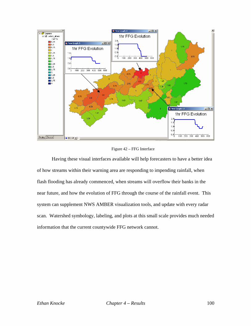
Figure 42 – FFG Interface

Having these visual interfaces available will help forecasters to have a better idea

of how streams within their warning area are responding to impending rainfall, when

flash flooding has already commenced, when streams will overflow their banks in the

near future, and how the evolution of FFG through the course of the rainfall event. This

system can supplement NWS AMBER visualization tools, and update with every radar

scan. Watershed symbology, labeling, and plots at this small scale provides much needed

information that the current countywide FFG network cannot.


5.0 Discussion and Conclusions

5.1 Achievement of Objectives

The primary goal of this thesis research was to take common hydrologic modeling

techniques and construct a GIS embedded FFG model from scratch utilizing the

programming languages available within the ArcGIS 8.3 platform. This model can serve

as a pilot example of how embedded GIS can remove the need for coupled hydrologic

modeling. The methodology, analysis, and results of this research achieved the three

objectives in section 1.2 that were used to meet this goal in the following ways:

• Investigate the ways in which embedded GIS modeling and analysis can

enhance the accuracy of ungaged small sub-watershed hydrologic modeling.

Simple proven hydrological modeling techniques (SCS-CN Method, SCS UH,

Muskingum stream routing) were programmed from scratch within the ArcGIS

8.3 Visual Basic environment using VBA and ArcObjects functionality. Input

variables were developed using the GIS analysis environment, rainfall was read

into the GIS model from AMBER text files, a series of .dbf tables were developed

and manipulated to track hydrograph evolution, two-dimensional arrays were

generated and altered for stream routing inventory, rainfall was converted into

direct runoff within the GIS framework, discharge hydrographs were developed,

FFG depths were assigned, and finally the symbology and graphing interface of

GIS was called to display model output. This model functions at a temporal scale

of five minutes to match NEXRAD radar output, and keeps an inventory of

discharge and FFG at the spatial scale of the small watersheds utilized within the

Ethan Knocke Chapter 5 – Discussion and Conclusions 101

AMBER software. Explanation of the model process and how it serves as an

improvement to the current FFG system can be found in sections 3.1 and 3.2.

• Test the effect that required input parameters for the hydrological formulas

have on the resulting FFG output, using sensitivity analyses.

Sensitivity analyses were performed on the SCS UH procedures and FFG model

output to determine the impact of elevation error on terrain related input variables

and AMC criteria on CN adjustments for model simulation.

Five random error elevation grids were developed from the source NED for the

elevation analysis. Then watersheds and streams were delineated for each

scenario, SCS UH equation parameters were re-computed to determine their

influence on Tp and Qp, and UH plots were generated for each elevation scenario.

It was found that error in elevation is insignificant within upstream watersheds

with well defined drainage divides and stream channels; while error was more

influential within wider downstream watersheds, near stream confluences, and in

watersheds dominated by rolling terrain and fuzzy boundaries. Drainage area and

length to divide were altered the most out of the parameters because they are

computed based on the shape of the terrain itself, while mean slope and CN are

not perturbed as much due to the high volume of interior grid cells involved in

their computation. Elevation error does have an impact on UH timing and shape,

and confidence intervals should be provided to reveal the uncertainty involved in

the SCS UH development. Further examination of the elevation sensitivity

analysis can be found within section 4.1.

Three AMC simulation techniques (Lit, AMCII, and AMCIII) were developed to


test the impact of CN alterations based on soil moisture conditions. Results reveal

that the literature based CN classifications and AMC adjustments used in this

research are sometimes ineffective in simulating the correct initial abstractions,

direct runoff levels, and hydrograph timing and magnitude. Isolated storm events

with dry AMC drop CN values so low that initial abstractions for this heavily

forested study area were never met in the simulations by the observed rainfall

depth. Storm events with marginal rainfall (zero to 0.5 inches) were not

simulated correctly by any of the three AMC scenarios, showing that runoff CN

classifications break down for weak storms. Extraordinary rainfall events (two to

four inches) tend to be overestimated in this model setup due to the heavy

dependence of the rainfall-runoff process on assigning the correct CN and time of

concentration. For simulations where AMC adjustments altered CN to a value

where direct runoff can commences, it was found through high cross correlations

that the model does do very well at determining the correct time that initial

abstractions should be nullified and how the rising side of the hydrograph should

evolve. There is also a trend toward early peaking hydrographs with overshooting

peak discharges within this model, and closer examination of AMC levels and

resulting CN, and time of concentration could solve this issue. An in depth

analysis of the performance of this hydrologic model within the ten storm events

can be found in section 4.2.

• Advance the methodologies involved in real-time FFG development by

performing statistical analyses on the results of the most accurate FFG.

Even though there was success in implementing a complete hydrologic FFG


model and flood analysis interface within the GIS framework and output FFG

now has the ability to update in real time with considerable accuracy, there are

still some shortcomings of the model process and assumptions that need to be

addressed. Model components that seem to impact hydrograph accuracy the most

include the subjectivity of CN computation, the uncertainty in current AMC

adjustment factors, the uncertainty in NEXRAD radar and AMBER MAP

accuracy, error in observed unit discharges at USGS streamgages, and the error

involved in pushing the limits of SCS UH theory to a five minute time scale.

Examining the simulated hydrographs for each storm event showed that there is

inconsistency in the accuracy of the five-day AMC CN assignment ranges (Table

4) and adjustment equations between AMC I and AMC III (3.4 – 3.6) currently

used in literature. Peak discharge simulations within the most accurate AMC

simulation for each storm were seven to 68 percent above or below the observed

peak and timing offsets existed anywhere from 0.5 to nine hours. This shows that

there is too much uncertainty in the impact that these subjective alterations have

on CN and AMC adjustments to runoff potential should be accounted for utilizing

a more complex soil moisture model. Verifying volume comparison of the

Muskingum stream routing procedure revealed that the routing functions coded in

this GIS model are accurate at conserving runoff water. This shows that out of

the two primary components of the model (SCS-CN and UH generation and

Muskingum routing), the main sources of error only come from the SCS

techniques and assumptions.


5.2 Conclusions

This research provides a pilot embedded GIS model for FFG development. In

order to program the hydrological processes necessary for effective FFG computation,

simple but common techniques were used to construct the model. The model has the

ability to process rainfall, runoff, stream discharge, and flash flood potential at the same

spatial scale as the AMBER watersheds every five minutes in order to keep consistent

with radar information. The graphical interface coupled with this model will

dramatically improve the amount of hydrologic and meteorological data available to

forecasters for flash flood forecasting purposes.

Model functionality is accurate in conserving excess runoff as it is routed from

headwaters downstream to the outlet. However, issues of CN classification, AMC

alteration, and UH generation within the SCS hydrograph procedures create uncertainty

in the development of a five minute storm hydrograph. With this model evolving every

five minutes for storm events approaching 12 hours in length, errors in each five minute

storm hydrograph can propagate and magnify as the storm event progresses. For FFG

purposes it is not necessarily important to match streamflow rates exactly, but critical to

simulate the relative time and magnitude of the peak discharge from a storm event. The

difference between this peak discharge and bankfull discharge is what determines FFG

depths and when flash flooding is likely to start. Hydrometeorologists can utilize these

two pieces of information along with meteorological rainfall models to predict when

streams have the potential to exceed their banks and issue flash flood warnings further in

advance.


In order to fix these offsets in hydrograph timing and peak discharge magnitudes,

the following model components should be assessed:

• Proper runoff CN classification for various storm types and characteristics

• Better methods of keeping a continuous inventory of AMC

• Better methods of interpolating the SCS UH to a five minute time step

• Accuracy of observed streamflow from USGS stream gages and of MAP

estimations from the AMBER software

• Comparison of required CN based on the observed gage hydrograph with CN

values used in the simulation for calibration purposes

• Comparison of observed peak discharge timing and magnitude with simulated

results to determine hydrograph shape adjustments

In conclusion, the embedded GIS capabilities that were developed within this

research have dramatically improved the application of FFG and flash flood forecasting.

This model removes the need for an external coupled hydrological model reducing the

amount of data development and transfer between software interfaces. Having all phases

of the FFG system (preprocessing, implementation, analysis, and output) centralized in

one GIS package will provide a better means of managing the model, tracking the success

of the model, calibrating and troubleshooting errors that maybe be found, and improve

the output delivery time and accuracy.

This model functions at a unit of analysis of watersheds on the order of 0.5 to 9.5

square miles in area instead of the current large basin scale. At this smaller scale, the

SCS UH techniques can be utilized instead of the current Snyder UH method. Having the

hydrological techniques and FFG processing at this fine scale is critical because this is


the same spatial scale of the NWS AMBER program. Therefore, the model has the

ability to simulate the rainfall-runoff process at the same unit of input MAP from

AMBER. Output FFG values are computed for each small watershed instead of

aggregating up to the county or zone scale. This added detail provides much needed

spatial information about the distribution of rainfall patterns, runoff patterns, streamflow

patterns, and flash flood threat patterns which can be reported only in those specific areas

that warrant the report rather than much larger units used today.

This model also functions at a temporal scale of five minutes, which is a drastic

improvement over the six hour time step used within the current system. Having the

ability to track runoff rates, stream levels, and FFG in real time with NEXRAD radar

information will add much needed information that the current six hour to daily FFG

update cannot provide. This increase in frequency of FFG updates will also help

forecasters to match FFG estimates in real time with NEXRAD rainfall depths and

meteorological rainfall forecast models, which will allow forecasters to identify flash

flood threat times and locations earlier and increase the amount of warning time provided

to the public.

The graphics interface of this model gives forecasters the ability to monitor a

variety of hydrological and flood related characteristics, some of which are currently not

available. These attributes include displaying rainfall totals, direct runoff totals, required

rainfall depths to reach saturation, storm event runoff CN, current simulated peak

discharge rates, current flash flood threat levels, and current one and three hour FFG.

Having the ability to plot rainfall distributions, simulated hydrographs, and FFG


evolution for each small watershed will help forecasters to visualize spatial variability in

runoff impacts for a storm event.

Though the benefits are clear, the process of embedding hydrological modeling

techniques within the GIS framework and stretching the limits of SCS and Muskingum

procedures to this small spatial and temporal scale did bring an element of uncertainty to

the rainfall-runoff process that is leading to error in hydrograph simulation for some

storm event types and conditions. Based on results, there is a trend toward a more rapid

ascent in the rising side of the storm hydrograph which can lead to an early peak at a

higher magnitude. Primary causes of this error are uncertainty in the subjectivity of CN

classification and AMC adjustments, as well as uncertainty in the accuracy of watershed

and stream delineation and terrain related parameters due to error in NED data. Further

analysis of rainfall input, rainfall-runoff processing, CN, AMC, and UH development at

this 5 minute small watershed scale will help to solve these issues.

5.3 Future Research

Now that a functional FFG model has been framed out within the GIS

environment, future research should address adjusting the components of this model that

are leading to error propagation through the simulation process. First, the memory

leakage issue that exists when the loop involved in this model approaches 250 iterations

needs to be addressed in order to simulate fully a storm event of any duration from initial

baseflow to the recession baseflow. Then full storm event hydrograph comparisons

should be performed to make sure that the simulated study area outlet hydrograph

contains the same total volume as the Shawsville streamgage hydrograph.


Improvements of runoff CN assignments can be pursued by computing observed

CN values needed to match the observed streamgage hydrograph and comparing them

with CN values used in this model. These comparisons can then be used to notice trends

that may exist in the differences between the model and observed CN. There are also CN

classification tables beyond the scheme used in this model (Table 3) and these

categorizations can be applied to the model to determine the CN classification that is

most effective.

Improvements in AMC accuracy can be achieved by removing the simplistic

five-day AMC CN adjustments and utilizing a more sophisticated soil moisture content

model like the Sacramento Soil Moisture Accounting (SACSMA) model or water balance

models. These models factor in not only antecedent rainfall totals, but also snowmelt,

evapotranspiration, groundwater recharge, and surface runoff rates. The runoff CN of a

watershed is critical in this model because it influences the UH Tp computation and the

SCS-CN rainfall-runoff relationship equations. Since the simulated AMC of a watershed

has the final say in CN characterization, it is critical to maintain the most accurate

inventory of soil moisture possible.

Rainfall accuracy of the AMBER software can be performed by correlating MAP

values with observed rain gage and IFLOWS records for small watersheds that contain

one of these gages. Also the SCS UH shape follows a gamma distribution, so

improvements in five minute UH development can be made by attempting interpolation

methods that go beyond simple linear interpolation to techniques such as a two or three

parameter gamma distribution. The underlying hydrologic modeling processes and FFG

development will also have to evolve from the current storm event mode to real-time so


that the model will be able to update every 5 minutes instead of simulating an entire

storm duration. Finally, even though it was found in this research that the simulated FFG

values in this GIS application can be accurate provided an effective rainfall-runoff model,

gaining access to NWS countywide FFG archives from the Ohio and Southeast RFC for

these events may still be helpful to check for overall consistencies and differences and/or

prove that this model is more accurate.


References

Battaglin, W.A., G. Kuhn, and R. Parker. 1996. Using GIS to Link Digital Spatial Data and the Precipitation Runoff Modeling System: Gunnison River Basin, Colorado. In GIS and Environmental Modeling, eds. M.F. Goodchild, L.T. Steyaert, B.O. Parks, C. Johnson, D. Maidment, M. Crane, and S. Glendinning, 159-163. Colorado: GIS World, Inc.

Bedient, P.B., and W.C. Huber. 2002. Hydrology and Floodplain Analysis, 3rd Edition.

New Jersey: Prince-Hall, Inc. Brimicombe, A.J., and J.M. Bartlet. 1996. Linking GIS with Hydraulic Modeling for

Flood Risk Assessment: The Hong Kong Approach. In GIS and Environmental Modeling, eds. M.F. Goodchild, L.T. Steyaert, B.O. Parks, C. Johnson, D. Maidment, M. Crane, and S. Glendinning, 165-168. Colorado: GIS World, Inc.

Burrough, P.A., R. van Rign, and M. Rikken. 1996. Spatial Data Quality and Error

Analysis Issues: GIS Functions and Environmental Modeling. In GIS and Environmental Modeling, eds. M.F. Goodchild, L.T. Steyaert, B.O. Parks, C. Johnson, D. Maidment, M. Crane, and S. Glendinning, 29-34. Colorado: GIS World, Inc.

Butts, M.B., J.T. Payne, M. Kristensen, and H. Madsen. 2004. An evaluation of the

impact of model structure on hydrological modeling uncertainty for streamflow simulation. Journal of Hydrology 298: 242-266

Carpenter, T.M., J.A. Sperfslage, K.P. Geogakakos, T. Sweeney, and D.L. Fread. 1999.

National Threshold Runoff Estimation Utilizing GIS in Support of Operational Flash Flood Warning Systems. Journal of Hydrology 224: 1-23.

Carsell, K.M., N.D. Pingel, and D.T. Ford. 2004. Quantifying the Benefit of a Flood

Warning System. Natural Hazards Review 5(3): 131-140. Choudhury, P., R.K. Shrivastava, and S.M. Narulkar. 2002. Flood Routing in River

Networks Using Equivalent Muskingum Inflow. Journal of Hydrologic Engineering 7(6): 413-419

DeVries, J.J. and T.V. Hromadka. 1995. Computer Models for Surface Water. In

Handbook of Hydrology, ed. D.R. Maidment, 22.1-22.34. New York: McGraw-Hill, Inc.

Dodson, R.D. 1995. Advances in Hydrologic Computation. In Handbook of Hydrology,

ed. D.R. Maidment, 23.1-23.24. New York: McGraw-Hill, Inc. Doswell III, C.A., H.E. Brooks, and R.A. Maddox. 1996. Flash Flood Forecasting: An

Ingredients-Based Methodology. Weather Forecasting 11: 560-581.

Ethan Knocke References 111

Engel, B.A. 1996. Methodologies for Development of Hydrologic Response Units Based

on Terrain, Land Cover, and Soils Data. In GIS and Environmental Modeling, eds. M.F. Goodchild, L.T. Steyaert, B.O. Parks, C. Johnson, D. Maidment, M. Crane, and S. Glendinning, 123-128. Colorado: GIS World, Inc.

Feldman, A.D. 1995. HEC-1 Flood Hydrograph Package. In Computer Models of

Watershed Hydrology, ed. V.P. Singh, 119-150. Colorado: Water Resources Publications.

Goodchild, M.F. 1994. Geographic Information Systems and Geographic Research. In

Ground Truth: The Social Implications of Geographic Information Systems, ed. J. Pickles, 31-50. New York: Guilford.

Goodchild, M.F. 1996. The Spatial Data Infrastructure of Environmental Modeling. In

GIS and Environmental Modeling, eds. M.F. Goodchild, L.T. Steyaert, B.O. Parks, C. Johnson, D. Maidment, M. Crane, and S. Glendinning, 11-15. Colorado: GIS World, Inc.

Goodchild, M.F. and P.A. Longley. 1999. The Future of GIS and Spatial Analysis. In

Geographical Information Systems Volume 1: Principles and Technical Issues, 2nd Edition, eds. P.A. Longley, M.F. Goodchild, D.J. Maguire, D.W. Rhind, 567-580. New York: John Wiley & Sons, Inc.

Haested, and S.R. Durrns, 2003. Stormwater Conveyance Modeling and Design, 1st

Edition. Waterbury, CT: Haestad Press. Hutchinson, M.F. and J.C. Gallant. 1999. Representation of Terrain. In Geographical

Information Systems Volume 1: Principles and Technical Issues, 2nd Edition, eds. P.A. Longley, M.F. Goodchild, D.J. Maguire, D.W. Rhind, 105-124. New York: John Wiley & Sons, Inc.

Kent, K.M., 1972. SCS National Engineering Hand-book, Section 4: Hydrology. Chapter

15: Travel Time, Time of Concentration, and Lag. U.S. Department of Agriculture. Washington, D.C.

Knocke, E.W. and K. Kolivras. 2005. Flash Flood Awareness in Southwest Virginia. In

Review by Risk Analysis International Journal Lam, D. and C. Pupp. 1996. Integration of GIS, Expert Systems, and Modeling for State-

of-Environment Reporting. In GIS and Environmental Modeling, eds. M.F. Goodchild, L.T. Steyaert, B.O. Parks, C. Johnson, D. Maidment, M. Crane, and S. Glendinning, 419-422. Colorado: GIS World, Inc.


Laurenson, E.M. and R.G. Mein. 1995. RORB: Hydrograph Synthesis by Runoff Routing. In Computer Models of Watershed Hydrology, ed. V.P. Singh, 151-164. Colorado: Water Resources Publications.

Leavesley, G.H. and L.G. Stannard. 1995. The Precipitation-Runoff Modeling System –

PRMS. In Computer Models of Watershed Hydrology, ed. V.P. Singh, 281-310. Colorado: Water Resources Publications.

Longley, P.A., M.F. Goodchild, D.J. Maguire, and D.W. Rhind. 1999. Introduction. In

Geographical Information Systems Volume 1: Principles and Technical Issues, 2nd Edition, eds. P.A. Longley, M.F. Goodchild, D.J. Maguire, D.W. Rhind, 1-20. New York: John Wiley & Sons, Inc.

Maguire, D.J. 1999. GIS Customization. In Geographical Information Systems Volume 1:

Principles and Technical Issues, 2nd Edition, eds. P.A. Longley, M.F. Goodchild, D.J. Maguire, D.W. Rhind, 359-369. New York: John Wiley & Sons, Inc.

Maidment, D.R. 1993. GIS and Hydrologic Modeling. In Environmental Modeling with

GIS, eds. M.F. Goodchild, B.O. Parks, and L. Steyaert, 147-167. New York: Oxford University Press.

Maidment, D.R. 1996. Environmental Modeling within GIS. In GIS and Environmental

Modeling, eds. M.F. Goodchild, L.T. Steyaert, B.O. Parks, C. Johnson, D. Maidment, M. Crane, and S. Glendinning, 315-323. Colorado: GIS World, Inc.

Mays, L.W. 2001. Water Resources Engineering, 1st Edition. New Jersey: John Wiley &

Sons, Inc. McCormick, B.C. 2003. Distributed Hydrologic Modeling of the Upper Roanoke River

Watershed using GIS and NEXRAD. Masters Thesis in Civil Engineering at Virginia Tech.

McEnroe, B.M., and P. Gonzalez. 2003. Storm Duration and Antecedent Moisture

Conditions for Flood Discharge Estimation. Report No. K-TRAN: KU-02-4, Final Report, 1-50.

Mishra, S.K., and V.P. Singh. 2003. Soil Conservation Service Curve Number (SCS-CN)

Methodology. Water Science and Technology Library Volume 42. Dordrecht: Kluwer Academic Publishers

Mockus, V., 1972. SCS National Engineering Hand-book, Section 4: Hydrology. Chapter

7: Hydrologic Soil Groups. U.S. Department of Agriculture. Washington, D.C. NCDC. 2005. U.S. Storm Event Database. WWW Document, < http://www.ncdc.noaa.gov/oa/climateresearch.html >


Nelms, D.L., G.E. Harlow Jr., and D.C. Hayes. 1997. Base-Flow Characteristics of Streams in the Valley and Ridge, the Blue Ridge, and the Piedmont Physiographic Provinces of Virginia. U.S. Geological Survey Water-Supply Paper 2457, 1-47.

NRC, 2005. Flash Flood Forecasting Over Complex Terrain: With an Assessment of the

Sulphur Mountain NEXRAD in Southern California. Washington D.C.: The National Academic Press.

NRCS, 2005. Regional Hydraulic Geometry Curves. WWW Document,

< http://wmc.ar.nrcs.usda.gov/technical/HHSWR/Geomorphic/ > NWS. 2004. AMBER Basin Files. Data provided by Paul Jendrowski, Information

Technology Specialist. NWS. 2005. National Weather Service Glossary. WWW Document,

< http://www.nws.noaa.gov/glossary/ > NWS. 2005. National Weather Service Climate. WWW Document, < http://www.weather.gov/climate/index.php?wfo=rnk > Pilgrim, D.H., and I. Cordery. Flood Runoff. In Handbook of Hydrology, ed. D.R.

Maidment, 9.1-9.42. New York: McGraw-Hill, Inc. Reed, S., D. Johnson, and T. Sweeney. 2002. Application and National Geographic

Information System Database to Support Two-Year Flood and Threshold Runoff Estimates. Journal of Hydrologic Engineering 7(3): 209-219

River Forecast Center Development Management Team (RFC). 2003. Flash Flood

Guidance Improvement Team Final Report. National Weather Service. Saghafian, B. 1996. Implementation of a Distributed Hydrologic Model within GRASS

In GIS and Environmental Modeling, eds. M.F. Goodchild, L.T. Steyaert, B.O. Parks, C. Johnson, D. Maidment, M. Crane, and S. Glendinning, 205-208. Colorado: GIS World, Inc.

Singh, V.P. 1995. Watershed Modeling. In Computer Models of Watershed Hydrology,

ed. V.P. Singh, 1-22. Colorado: Water Resources Publications. Sorrell, R.C. 2000. Computing Flood Discharge For Small Ungaged Watersheds.

Michigan Department of Environmental Quality Land and Water Management Division.

Snider, D. 1972. SCS National Engineering Hand-book, Section 4: Hydrology. Chapter

16: Hydrographs. U.S. Department of Agriculture. Washington, D.C.


http://www.nws.noaa.gov/glossary/

Srinivasan, R., J. Arnold, W. Rosenthal, and R.S. Muttiah. 1996. Hydrologic Modeling of Texas Gulf Basin Using GIS. In GIS and Environmental Modeling, eds. M.F. Goodchild, L.T. Steyaert, B.O. Parks, C. Johnson, D. Maidment, M. Crane, and S. Glendinning, 213-217. Colorado: GIS World, Inc.

Steyaert, L.T., 1996. Status of Land Data for Environmental Modeling and Challenges

for Geographic Information Systems in Land Characterization. In GIS and Environmental Modeling, eds. M.F. Goodchild, L.T. Steyaert, B.O. Parks, C. Johnson, D. Maidment, M. Crane, and S. Glendinning, 17-27. Colorado: GIS World, Inc.

Sweeney, T.L. 1992. Modernized Areal Flash Flood Guidance. NOAA Technical

Memorandum NWS Hydro 44. Silver Spring, MD. Sweeney, T.L., D.L. Fread, and K.P. Georgakakos. 1993. GIS Application for NWS

Flash Flood Guidance Model. Sweeney, T.L. and T.F. Baumgardner. 1999. Modernized Flash Flood Guidance. WWW

Document, <http://www.nws.noaa.gov/ohd/hrl/ffg/modflash.htm> USGS. 2004. The National Map Seamless Data Distribution System. WWW Document,

< http://seamless.usgs.gov/ > USGS. 2005. USGS Shawsville Streamflow Files. Data provided by Shaun Wicklein,

Supervisory Hydrologist. USGS. 2005. USGS Surface Water for USA: Peak Streamflow. WWW Document, < http://nwis.waterdata.usgs.gov/usa/nwis/peak > USGS. 2001. The National Flood Frequency Program – Methods for Estimating Flood

Magnitude and Frequency in Rural Areas of Virginia. USGS Fact Sheet 023-01, February, 2001


Vita

Ethan Knocke was born in Blacksburg, Virginia on April 8, 1982. He developed

a passion for the weather at an early age and started his journey toward a career in

meteorology by receiving a Bachelor of Science in Meteorology from the Pennsylvania

State University in December 2003. During his undergraduate studies, he realized the

importance of spatial analysis in weather forecasting and earned a minor in GIS. He then

pursued further education in GIS at Virginia Tech to earn a Masters of Science in

Geography. During his Master’s studies he was a graduate research assistant with the

Center for Geospatial Information Technology (CGIT) and also served as a teaching

assistant for an online meteorology course. Ethan is now beginning a career that focuses

on linking GIS with meteorology and related sciences.

Ethan Knocke Vita 116

Modeling Flash Floods in Small Ungaged Watersheds using ...

Documents

Transcript of Modeling Flash Floods in Small Ungaged Watersheds using ...