1

Modeling Escape from a One-Dimensional Potential Well at Zero or Very Low Temperatures

Chungho Cheng

Department of Mechanical and Aerospace Engineering, University of California, Davis, California 95616, USA

Gaetano Salina

Istituto Nazionale di Fisica Nucleare, Sezione Roma “Tor Vergata”, I-00133 Roma, Italy

Niels Grønbech-Jensen

Department of Mathematics and Department of Mechanical and Aerospace Engineering, University of California, Davis, California 95616 , USA

James A. Blackburn

Physics & Computer Science, Wilfrid Laurier University, Waterloo, ON N2L 3C5, Canada

Massimiliano Lucci and Matteo Cirillo (*)

Dipartimento di Fisica and MINAS-Lab Università di Roma “Tor Vergata”, I-00133 Roma, Italy

Abstract

The process of activation from a one-dimensional potential is systematically investigated in

zero and nonzero temperature conditions. The features of the potential are traced through

statistical escape from its wells whose depths are tuned in time by a forcing term. The process is

carried out for the damped pendulum system imposing specific initial conditions on the potential

variable. While the escape properties can be derived from the standard Kramers theory for

relatively high values of the dissipation, for very low dissipation these deviate from this theory

by being dependent on the details of the initial conditions and the time dependence of the forcing

term. The observed deviations have regular dependencies on initial conditions, temperature, and

loss parameter itself. It is shown that failures of the thermal activation model are originated at low

temperatures, and very low dissipation, by the initial conditions and intrinsic, namely T=0,

characteristic oscillations of the potential-generated dynamical equation.

(*) Corresponding author : cirillo@roma2.infn.it

2

1) INTRODUCTION

The interest for fluctuations in dynamical systems and the analysis of their dynamical response

when subject to external forcing terms and/or thermal noise is a subject that has attracted generations

of scientists. Several relevant reviews are available on this topic [1, 2, 3] and body of work and insight

are still expanding in part due to increased power of numerical techniques. A key model for describing

thermal activation is due to Kramers [4,5]; a relevant feature of this model is that the escape rate Γ

from a potential well with amplitude ∆U, at temperature T, is governed by the equation [4]

Γ = 𝑓𝑓 exp(−Δ𝑈𝑈𝑘𝑘𝐵𝐵𝑇𝑇

) (1)

where f is an attempt frequency. A system to which Kramers model (and eq. 1) has been

extensively applied is the compound pendulum, which is described by the following normalized

equation for the angle φ

�̈�𝜑 + 𝛼𝛼�̇�𝜑 = −𝑑𝑑𝑈𝑈𝑑𝑑𝜑𝜑

(2)

with 𝑈𝑈(𝜑𝜑) = (1 − 𝑐𝑐𝑐𝑐𝑐𝑐𝜑𝜑) − 𝜂𝜂𝜑𝜑 being the potential energy. The coefficient α and the parameter η

account respectively for dissipation and forcing terms. Two recent reviews [6,7] demonstrate the

relevance of the system (2) in the history of physics and of show its intriguing counterparts in general

physics and nonlinear dynamics. In condensed matter the driven-damped pendulum equation is

analogous to that of the Josephson junction [8], which has been the focus of much attention in

theoretical, experimental, and applied physics level for decades [9,10]. Specific applications of

Kramers analysis to Josephson potentials were reported in two key publications by Kurkijarvi [11]

and Büttiker et al. [12].

Due to the applicability of Kramers model to a broad class of systems, we have conducted a

systematic statistical analysis of its validity for describing the behavior of the pendulum. We first

study, in the next section, the potential in the absence of temperature fluctuations, i. e. studying eq.

3

2 in absence of noise. In this T=0 case we focus on the dependence of the escape from the potential

for different values of dissipation values while increasing the force term linearly on time. We study

the effect of specific initial conditions on the statistical distributions of the escape processes analyzing

the response induced by the initial data. We also present a model which explains the underlying

physics of the obtained numerical results. Then, in sect. 3, we include thermal effects through a noise

term in eq. 2. We show that the conclusions made for the zero-temperature case about the initial

conditions can play a crucial role for the escape statistics in regime of low dissipation and nonzero

temperature. In sect. 4 we discuss the results in terms of experimental phenomenology while in sect.

5 we summarize the paper.

4

2) ZERO TEMPERATURE

In Fig. 1a the curves show the first well of the potential U that we are investigating traced for

increasing values of the parameter η (η = 0.6 , the lowest and η = 1 the highest). The inset shows the

value of the height of the potential barrier ∆U , the energy spacing between the maximum and minimum

value in the well, spanned over the entire interval [0;1] of the forcing term η ; according to the

dependence ∆𝑈𝑈 = 2(�1 − 𝜂𝜂2 − 𝜂𝜂𝑐𝑐𝑐𝑐𝑐𝑐−1𝜂𝜂), the depth of the potential (the difference in energy

between successive minimum and the maximum) decreases and goes to zero for η =1 as shown in

the inset. In our escape experiments and numerical procedures the forcing term is increased according

to 𝜂𝜂(𝑡𝑡) = �̇�𝜂𝑡𝑡 where the derivative �̇�𝜂 = 𝑑𝑑𝑑𝑑𝑑𝑑𝑑𝑑

is kept constant and the curves in Fig. 1a, in practice,

correspond to successive time shots for �̇�𝜂 = 1.95 x 10-8. In the figure we also indicate the stable

equilibrium points at the bottom of the potential (full diamonds) and the unstable (empty circles)

equilibrium points at the top of the well: these were calculated, for each curve evaluating numerically

the minima and the maxima.

In Fig. 2 we trace both stable and unstable equilibrium points as a function of η , respectively

by the continuous and the dashed lines: the crossing of the two curves is the point where an escape

event is recorded: we see that this event occurs, always when η =1 , when the well becomes flat and

the two curves cross, meaning that the stable and unstable equilibrium point have the same (η,ϕ)

coordinates. The escape event is numerically identified by the fact that, for a further increase of the

forcing term above η=1 , the system is driven in a dynamical condition of continuous phase increase

(rotation states in terms of the compound pendulum). For T=0 (zero temperature) and initial

conditions 𝜑𝜑0 = 𝜑𝜑(𝑡𝑡 = 0) = 0 and �̇�𝜑0 = 𝑑𝑑𝑑𝑑𝑑𝑑𝑑𝑑

(𝑡𝑡 = 0) = 0 , the escape from the potential well always

occurs for η=1 ; moreover, for these initial conditions, this situation remains the same, for any value

of α and η. The two plots in Fig. 2a,b represent indeed the results of the numerical integration for

these initial conditions and different values of α (indicated in the plot) : we can see that, even

5

decreasing the loss parameter of six orders of magnitude, the response is always the same and the

escape always occurs above η =1.

Before proceeding, however, it is necessary to specify what is our criterion to judge that an

escape process out of the potential well has safely occurred. When η < 1 the escape occurs at the

angle 𝜑𝜑 = 𝜋𝜋 − arcsin 𝜂𝜂 while for η ≈1 the escape is recorded when 𝜑𝜑 = 𝜋𝜋2 . In both cases the escape

from the well is double checked by the continuous increase of the phase generating a non–zero

average value of the time derivative of the phase (we usually stop the integration when < �̇�𝜑 >= 1 ).

The results herein presented have been obtained integrating the system (2) by specific versions of the

velocity-explicit Størmer-Verlet algorithm [13] setting the integration time ∆t =0.02 ; two

independently developed versions of the algorithm, running on different computers and operating

systems, always returned the same results. Halving tests for the integration time step were performed

routinely in order to check the independence of the results upon it.

Keeping the same value of �̇�𝜂 = 1.95𝑥𝑥10−8 but setting nonzero values for the initial angle 𝜑𝜑0

the dependence on the loss parameter of the escape process becomes significant and the values of η

for which escape from the potential well are recorded can be substantially different. Fig. 3 and Fig.

4 show two escape processes obtained both for initial condition 𝜑𝜑0 ≠ 0 (respectively ϕ0 =0.3π and

ϕ0=0.6 π for Fig. 3 and Fig. 4) and three decreasing values of the loss parameter α . The value of

time derivative of the initial phase �̇�𝜑0 was set to zero. The physical meaning of these initial conditions

for the system (2) corresponds to start an integration in an oscillating regime with zero average phase

derivative in the point where the phase has its maximum value and the derivative of the phase is zero,

namely the inversion point of the oscillations. We see now that in Fig. 3a,b and 4a,b the “phase

trajectory” still escapes from the potential well for η values very close to the critical one (the unity),

however, for α in the 10-7 range the phase oscillations due to the initial angle do not damp out and

the dark area in the figures is just generated by the oscillations whose period is too small to be seen

in the figures (we just show a zoom with few periods before escaping in the inset of Fig. 4b). In this

6

case the escape occurs, as shown in the figure, when the phase oscillation trajectory crosses the

unstable point trace for η <1 . Considered the effect shown in Fig. 3 and Fig. 4, we decided to

investigate systematically the effect of dissipation and initial conditions on the escape current, namely

the value of the bias current for which the system escapes from the well.

The result of our simulations for the dependence of the escape current upon loss parameter

and initial angle are epitomized in Fig. 5. Here we show in a three-dimensional plot the data obtained

for the escapes out of the potential well of the system (2) for T=0 setting �̇�𝜂 = 1.95 x10-8 . On the

vertical axis we report the observed value of the “escape” of ηΕ , namely the value of η generating

an escape event from the periodic oscillations in the potential well to an out of the well running state

in which the angle increases continuously. On the horizontal axes we have the initial angle 𝜑𝜑0 which

is indicated in the figures as ϕ0 and the loss parameter α . We can see that when the initial angle tends

to zero the escape always occurs for ηΕ=1 , for any value of the loss parameter. Instead, when the loss

decreases and the initial angle increases we see that the escape current decreases substantially until it

reaches zero actually when 𝜑𝜑0 = ±𝜋𝜋 and values of the loss parameter less than 10-7. Changing the

value of the parameter �̇�𝜂 of one order of magnitude no substantial differences are observed in the

escape plots of Fig. 5: we always see that relevant changes occur below 𝑙𝑙𝑐𝑐𝑙𝑙𝛼𝛼 ≅ −7 .

In Fig. 6 we show two section of plots like that of Fig. 5 where we can see more clearly the

effect of the loss parameter condition (a) and initial conditions (b): these are used as parameters for

the curves in the figures where, on the vertical axis we always report the value of the escape current.

Both these “sections” were obtained for �̇�𝜂 =1.95x10-8. In (a) we can clearly see that the escape is very

flat down to 10-7 and then it becomes a monotonically decreasing and symmetric function of the angle

. Decreasing the loss, the width of the bell-shaped function shrinks but saturates for logα =-9. In (b)

we show the dependence of the escape current upon the parameter α for different initial conditions :

here we plot the escape current versus the log α and we parametrize with respect to the initial angle

7

and the result of this operation is just to set the value of a specific escape current on the left side of

the plot while on the right side, for α >10-7 , the escape current is always equal to the unity.

We then investigated the response of the system by changing the parameter �̇�𝜂 for a given initial

angle, 𝜑𝜑0 = 0.2 𝜋𝜋 and different values of the loss parameter. The results are shown in Fig. 7: here in

(a) we see that variations in �̇�𝜂 even of one order of magnitude, generate slight differences in the

escape currents around the loss values of the order of 10-7; the interesting thing now is to consider

what happens if we scale the horizontal axis of the data in (a) plotting the escape current as a function

of the common logarithm of ratio 𝜅𝜅 = 𝛼𝛼�̇�𝑑 . Now we find (see Fig. 7b) that all the data collapse in a

single curve. The data show that 𝜅𝜅, the ratio between loss parameter (α) and rate of increase of the

forcing term (�̇�𝜂), plays an important role providing a sort of normalization of the observed potential

escape features and a discontinuity in the response of the system occurs when 𝜅𝜅 = 1. The result of

Figs. 2-7 summarize our investigations for T=0 : given a specific initial condition on the angle

coordinate of the potential, the value of η for which we observe escape out of the potential well

depends in a relevant way from the values of the parameters α and �̇�𝜂.

We conclude that the system (2) undergoes an abrupt “transition” when 𝜅𝜅, the ratio between

dissipation and rate of increase of applied force, is equal to the unity. This ratio has also been shown

to play a relevant role in the context of the appearance of multipeaked escape statistical distributions

when sweep rates are particularly high [14,15]. Since we limit the investigation herein to statistical

distributions obtained with relatively low sweep rates, multipeaked distributions like those reported

in ref. 14 are not observed. As we shall see now the analysis for T=0 of the escape process is a

relevant physical background for understanding thermal excitations in the well. This is not surprising

indeed because it is known that the characteristics of a nonlinear system for T=0 leads to identifying

relevant phenomena [7] and it has been shown how complex can be the T=0 spectrum of “simple”

nonlinear systems [16] and how anharmonic analysis of the potentials can provide account for

experimental results [17].

8

In terms of Josephson effect physics the role of the oscillations generated by an initial angle

on the escape value ηE (the current for which the junctions switch from zero to non-zero voltage

state) can be understood, for low dissipation values, on the basis of a model for the energy stored in

the Josephson inductance in the zero voltage state. Given the value of the maximum Josephson pairs

current Ic the Josephson inductance is defined by [9]

𝐿𝐿𝐽𝐽 =1

�1 − ( 𝐼𝐼𝐼𝐼𝑐𝑐)2

𝛷𝛷0

2𝜋𝜋𝐼𝐼𝑐𝑐 (3)

Where I is the bias current fed through the junction and Φ0=2.07x10-15 Wb is the flux quantum.

In the limit I=0 the above equation returns the zero-bias Josephson inductance LJ0 = Φ0 /2πIc.

An initial angle ϕ0 gives rise, according to the Josephson dc equation, to an initial current in

the form I0 = Ic sin ϕ0 . We assume that, for t >0 , an oscillating current with amplitude I0 and

oscillating time dependence in the form I0 sin ωj t will be activated. Here we can consider ωj as the

bias-dependent Josephson angular plasma oscillations frequency [9]. In this harmonic approximation

it is straightforward to calculate the average energy in one period of these oscillations in the Josephson

inductor as 𝑊𝑊𝐿𝐿 = 14𝐿𝐿𝑗𝑗𝐼𝐼02.

We presume that, when damping is very low this initial energy will persist in the system even

when the value of the forcing term is slowly increased and indeed these oscillations are those that

we can see in the inserts of Figs. 3 and 4. Thus, the just calculated WL will contribute to lower the

barrier height ∆U of the washboard potential in one period in which an escape attempt occurs. We

recall now that in the expression for ∆U given before, in Josephson terms, energies are normalized

to the Josephson zero bias energy, namely EJ =Φ0Ic/2π. Normalizing WL to this quantity and

subtracting it from ∆U we get an effective height of the potential ∆UE in the form :

9

Δ𝑈𝑈𝐸𝐸 = 2 ��1 − 𝜂𝜂2 − 𝜂𝜂𝑐𝑐𝑐𝑐𝑐𝑐−1𝜂𝜂� − 𝜂𝜂02

4�1 − 𝜂𝜂02 (4)

where η0=I0/Ic = sin ϕ0 is the initial, normalized, current amplitude. From this equation the

value of η=I/Ic for which the escape to the voltage state in a Josephson junction occurs can be easily

evaluated as the value ηΕ for which ∆UE goes to zero. A comparison of such a calculation with the

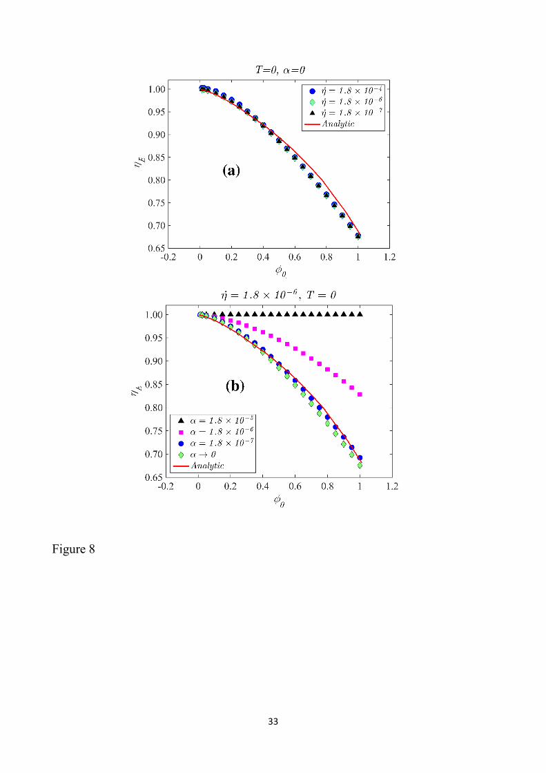
numerical data is shown in Fig. 8.

In Fig. 8a we have compared the analytical prediction obtained from (4) with the numerical

data for values of �̇�𝜂 , the current sweep rate in Josephson terms, varied over three orders of magnitude

setting α = 0 (the analytical calculation, in principle, is valid in this limit): we see that the agreement

between equation (4) and numerical data is very good for 0 ≤ ϕ0 < 1 . In Fig. 8b instead we investigate,

for a fixed value of the sweep rate, �̇�𝜂 = 1.8𝑥𝑥10−6, the effect of different values of the dissipation on

the escape current. We see here that the agreement between the predictions and the numerical is very

good when α is lower than the sweep rate, the condition in which we are observing the relevance of

the initial conditions. This confirms the relevance of the parameter κ and the physical nature of the

phenomenon generating early escapes which are due to the extra energy pumped in the system by the

initial condition when κ <1. In these conditions we see that the proposed lowering of the potential

predicted by eq. 4 gives a very good prediction of the escape current. Note in Fig. 8b that, for a given

value of the sweep rate, when a “saturation” value of α is reached (below the normalized sweep

rate) further lowering of it does not produce relevant changes in the escape current. For high values

of the loss parameter, as epitomized in Fig. 5 there are no changes of the escape currents and the

escape value always equals 1.

10

3) NON-ZERO TEMPERATURE

Let us step now to the analysis of the escape process for nonzero temperatures. Thermal

fluctuations are plugged into the right hand side of eq. 2 by the term 𝑛𝑛(𝑡𝑡) linked to the dissipation

through the fluctuation-dissipation relationship [18]: < 𝑛𝑛(𝑡𝑡) >= 0 and < 𝑛𝑛(𝑡𝑡)𝑛𝑛(𝑡𝑡′) > =

2 𝛼𝛼 𝑘𝑘𝐵𝐵𝑇𝑇𝐸𝐸

𝛿𝛿(𝑡𝑡 − 𝑡𝑡′), where T is the thermodynamic temperature of the system, kB =1.38 x10-23 J/K is

Boltzmann’s constant and E an adequate normalizing energy (in Josephson effect terms this is just

the EJ introduced in the past section). In Fig. 9a we show three statistical escape distribution obtained

for five values of the parameter 𝑘𝑘𝐵𝐵𝑇𝑇𝐸𝐸

which were, from left to right respectively 1.8x10-2, 1.3x10-2,

8.0x0-3, 4.0x10-3, 2.0x10-3, 5.0x10-4 . These distributions were obtained by setting the initial conditions

ϕ0 = 0 and �̇�𝜑0 = 0 , with standard deviation around these values given by (kBT/E)1/2, and setting

α =0.018 and �̇�𝜂 = 1.8𝑥𝑥10−9 .

Technically, the distributions of Fig. 9a are obtained generating 1500 escape events by

increasing η and recording each time the value of it for which the escape occurs : on the vertical axis

we just have the number of events (switches) relative to the specific η value. The horizontal

resolution is 6.4 x10-5 <∆η < 5.3x10-4 and it is varied depending on the width of the specific statistical

distribution. On the vertical axis we have essentially a probability distribution ρ expressed in

arbitrary units. The distributions move right with temperature and the width of the statistical

distributions decreases with temperature. In Fig. 9b we show the temperature dependence of the

widths of the statistical distributions for the same value of �̇�𝜂 = 1.8𝑥𝑥10−6 but for five different

values of the loss factor α which are one order of magnitude apart starting from 1.8x10-4 down to

1.8x10-8. We see that the dependencies are straight lines in a log-log plot (here we consider only the

data returning linear correlation coefficients above 0.999) and the values of the slope return the value

of the exponent γ of the power law indicated in the inset which varies in the interval [0.59;0.70].

Kramers theory (see eq. 12 of ref. 11, the paper is devoted to Josephson phenomenology) predicts a

11

dependence σ ≈ (kB T/ EJ)2/3 of the width of the statistical distributions on temperature; we see that only

one straight line of the log-log plot returns a value close to 2/3 while the other values are different up

to 10% from this value.

In Figure 9c we show the dependence of the slope of the straight lines of Fig. 9b, namely the

exponent γ of the law 𝜎𝜎 = (𝑘𝑘𝐵𝐵𝑇𝑇𝐸𝐸

)𝛾𝛾 , upon the parameter κ. We see that the slope of the curves has a

maximum around κ =1 and is roughly symmetrical around this point. Thus, the dynamical response

changes significantly as a function of the ratio a 𝛼𝛼�̇�𝑑 and, since the value of the sweep rate is fixed,

the result indicates that is the damping parameter which regulates the response of the system.

Analogous results can be obtained varying �̇�𝜂.

In Fig. 10a we show a plot similar to that of Fig. 9b obtained now setting a given angle as

initial condition, but still initial angular velocity set to zero, namely ϕ0 = 0.2π and �̇�𝜑0 = 0 . For the

two lower values of the loss parameter (1.8x10-7 and 1.8x10-6) we obtain the same value of the exponent

of the power law γ, within few parts over 103 uncertainty, and this value is equal to 0.5. The fitting

for the highest loss value instead (1.8x10-5) returns the exponent 0.672. In Fig. 9b we show the

dependence of the exponent γ of the law 𝜎𝜎 = (𝑘𝑘𝐵𝐵𝑇𝑇𝐸𝐸

)𝛾𝛾 upon logκ . We see here, more clearly than in

Fig. 9c, that the response of the system exhibits abrupt differences below and above 𝜅𝜅 = 1. It is worth

noting that the same dependence shown in Fig. 10b, is recorded if we set a different angle as initial

condition: along with 𝜑𝜑0 = 0.2 𝜋𝜋 we tested the results for and 𝜑𝜑0 = 0.5 𝜋𝜋 and 𝜑𝜑0 = 0.1 and these

cases returned exactly the same dependence in the range of logκ shown in Fig. 9b . We conclude

that the effect of setting a given angle as initial condition is to generate, for 𝜅𝜅 < 1, a straightforward

dependence of the standard deviation of the statistical distributions upon the square root of the

temperature 𝜎𝜎 = �𝑘𝑘𝐵𝐵𝑇𝑇𝐸𝐸

valid at least over two orders of magnitude of the parameter 𝑘𝑘𝐵𝐵𝑇𝑇𝐸𝐸

.

12

If we now choose as initial condition an angle distributed randomly and uniformly in a given

interval [-ϕ0;ϕ0], the above found square root dependence of the standard deviation of the

distributions upon kBT/E fails. What happens in this case quantitatively evident in Fig. 11a,b,c where

we show the dependence of the standard deviation of the distributions upon the normalized thermal

energy in a log-log plot. Here we see that for lower values of the normalized energy a saturation of

the standard deviation occurs and the specific saturation current depends on the initial angle. The

result are obtained setting an initial angle randomly uniformly distributed respectively in the intervals

[-0.1;0.1] (a) , [-0.2π ;0.2π] (b) and [-π/2;π/2] (c). In the plots we also show the dependence of the

“saturation” curves upon the loss parameter. Looking back at the T=0 results we can have a

straightforward explanation of this effect considering, in particular, Fig. 6b. We see there that

different initial angles correspond to different escape currents and therefore if the initial angle is

uniformly distributed over an interval the escape ηΕ also shall be distributed over an interval which

will set a distribution even for T=0. When the temperature in the system is high enough these initial

condition-generated oscillations shall not be visible because are masked by thermal fluctuations,

however, when thermal fluctuations have a low energy the standard deviation is just determined by

the randomness of the initial angle distribution.

In Figs. 11a,b,c we also write the slopes of the “linear” portions of the plots, those

corresponding to higher temperatures. It is worth noting that results similar to those of Fig. 10,

obtained setting an initial uniform random distribution of the angle can be obtained even with

different type of random initial conditions.

The above argument concerning the saturation of the standard deviation of the escape

distributions based on the T=0 behavior, makes sense when κ is of the order of the unity and below.

When κ is much above the unity the distribution of escape values does not depend on the initial angle,

as we see in Figs. (3-7), and therefore saturation cannot be expected on the basis the above conjecture.

However, in the nonzero temperature case variations of the plots of Figs. (3-7) can be expected and

13

saturations effects are recorded even at very low temperatures even for κ >1, as shown in Fig. 11. We

see in this figure that the “saturation” σ -value of statistical distribution at low energies/temperatures

depends on the amplitude of the random initial angle interval and on the value of the loss parameter.

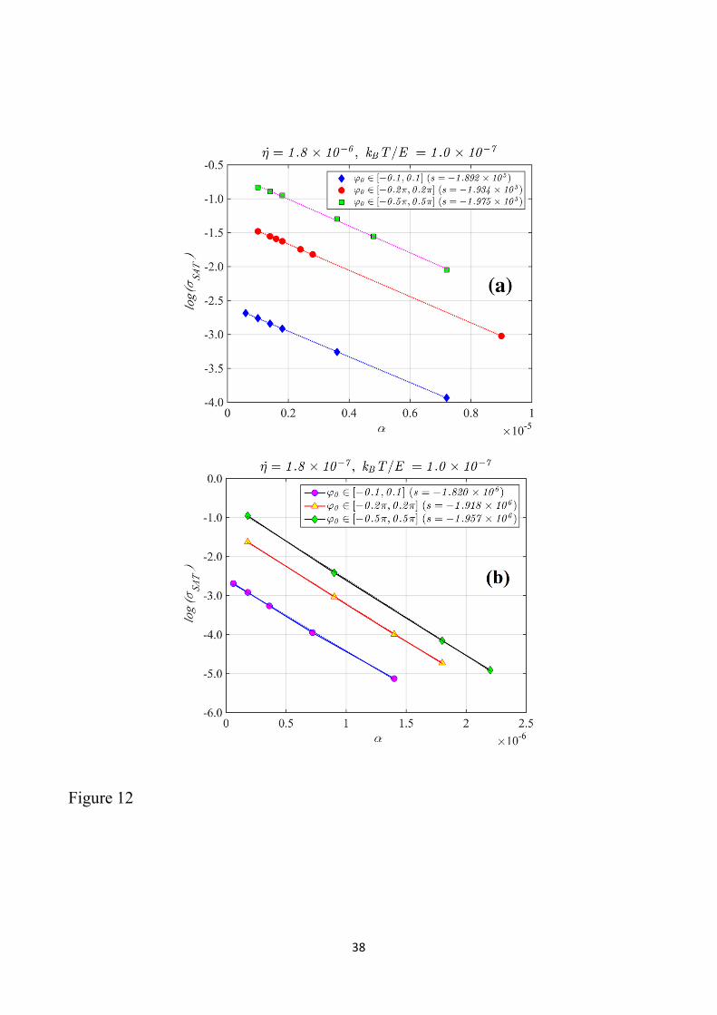
We have seen in Fig. 11 that, for a given value of �̇�𝜂 the with of the distributions can attain a

saturation value that will call σSAT . In Fig. 12 we show the dependence of this parameter upon the

loss parameter α in a semi-logarithmic plot for three settings of the initial conditions corresponding

to have the angle uniformly distributed respectively in [-0.1; 0.1], [-0.2π;0.2π] and [-0.5 π ; 0.5 π]:

Fig. 12a has been obtained for �̇�𝜂 = 1.8 𝑥𝑥 10−6. Instead, in Fig. 12b we show the same dependencies

of the saturation currents, for the same initial conditions, obtained for �̇�𝜂 = 1.8 𝑥𝑥 10−7. We clearly

see that both 12a,b that the dependencies are exponential of the type 𝜎𝜎𝑆𝑆𝑆𝑆𝑇𝑇 = 𝜎𝜎0𝑒𝑒−𝑠𝑠𝛼𝛼 with slopes s,

indicated in the insets, which have only few percent differences between the two cases (for the same

random initial interval) . For both cases we see that the extrapolation of the straight lines toward α =

0 is a well defined, non zero, value and therefore, for a random initial angle the width of the

distribution has a finite value in a lossless system. “Parental” results of those shown in Fig. 12a,b

were recently obtained in ref. 14 for the width of the peaks appearing in the statistical distributions

for high sweep rate: in that case the dependence of the width of the individual peaks of a multipeaked

distribution was investigated and it was shown that the dependence of the width of the peaks on the

loss factor was exponential.

14

4) EXPERIMENTAL BACKGROUND

We note that the work herein contained is referred to very adiabatic changes of force terms in the

system (2). The effects of “pulsed” excitations on this system have been thoroughly investigated in

previous publications (see [10] and references therein). The pulsed experiments on our systems, and

the oscillations these generated are much reminiscent of the phenomenology early observed in pulsed

laser experiments [19]; in the present paper, however, we have undertaken a systematic analysis of

the “adiabatically” driven system (2) since we believe this effect can serve as useful background of

knowledge for investigating more complex and non adiabatic conditions. This was the case indeed

of the work recently appeared in ref. 14 for which a guide from (preliminary) results herein presented

was important.

Framing of our results in terms of experimental parameters and procedures can be illustrated for

a specific case. Systems which have represented a benchmark for the one-dimensional potential

herein treated are Josephson junction and interferometers (consisting of a superconductive loops

closed by one or two junctions). The first thing to point out is that the operating temperatures at which

Josephson systems have been typically operating have gone from 4.2K down to 10mK. What we have

used as normalizing energy E is, in Josephson terms, the zero-bias Josephson energy which is the EJ

defined earlier in sect.2. Now, typical maximum pair currents for the thermal activation experiments

performed on Josephson junctions are in the range (1-330)µA [20-26]. If we consider for example a

1µA Josephson current, the corresponding Josephson energy is EJ = 0.33 x10-21J and our normalized

kBT/EJ will be 0.16 at 4K and 4x10-4 at 10 mK. When the Josephson maximum current scales up one

order of magnitude the energy will scale up of the same amount and the maximum and minimum

values of the normalized energy will consequently scale down a factor 10. Thus, for a Josephson

current of 100 µA the energy EJ = 33 x10-21 J and the normalized temperature will range from 0.16 x

10-2 at 4 K down to 4x10-6 at 10 mK.

15

From the above estimate of currents and related normalized energy it is evident why we have

chosen the intervals of energy variation for our investigation. Other relevant parameters in our work

are the rate of change of the applied force �̇�𝜂 and the loss factor α ; as far as the first parameter is

concerned, also known in Josephson terms as normalized sweep rate since it is the normalized time

derivative of the bias current, this can vary from the range of 10-6 down to the range of 10-9, depending

on junctions properties (essentially capacitance and critical current) [20-25]. A special problem

instead is represented by establishing the effective losses in Josephson systems when performing

potential escape measurements; in this case the work reported in ref. 27, for example, provides

interesting information because it evaluates a specific temperature dependence of the dissipation in

the junctions and simulations should take into account this physical condition. An analysis of the

intriguing effects generated by the variations of this parameter would be interesting and requires

further investigations.

In the present work we have preferred to set constant the dissipation parameter α in order to

maintain our analysis more general because in many physical cases the dissipation coefficient can

just be kept constant. As we have seen at the beginning setting a constant dissipation factor and all

zero initial conditions there are no effects on the escape from the potential and the data indeed might

follow very accurately the Kramers model. In Fig. 13 we plot the numerically obtained position (in

current) of the statistical distribution peaks with initial phase and phase derivative set to zero, for

α=0.01 . The full circles represent the numerical results for the position in current of the statistical

peak of the distributions, in values normalized to Ic while the continuous line represents the prediction

of Kramers theory [28]. According this theory the position, in current (Ip), of peak of the statistical

distribution moves away from the T=0 Josephson critical curent Ic following the same functional

dependence on temperature of the width of the distribution, namely (Ic - <Ip>)/Ic≈ (kBT/Ej)2/3. A

numerical evidence of the fact that peak widths and position follow the same temperature dependence

16

is given in Fig. 51, right panel, of ref. 10 : as we see there, for the given value of the loss, the data

follow perfectly Kramers predictions all over the temperature range.

However, if the loss factor α is scaled down to 10-10 , namely below �̇�𝜂 = 2𝑥𝑥10−9 , so that the

parameter 𝜅𝜅 = 𝛼𝛼�̇�𝑑 is below the unity, at low temperatures the position of the peaks freezes as shown

by the yellow triangles in Fig. 13. For this specific run we have chosen to set “Gaussian” initial

conditions meaning that the initial angle is randomly distributed around the given angle ϕ0 = 0.0856 π

with a standard deviation of the packet proportional to the square root of the kBT ; the initial phase

derivative is always set to zero. The triangles, the squares and diamonds in Fig. 13 correspond to the

time steps of the numerical integration indicated in the inset, showing stability of the results, for very

low dissipation, under “halving” tests. The intersection of horizontal line obtained for α =10-10 with

the Kramers curve occurs for a temperature slightly above 50 mK. We can say that an initial angle

ϕ0 = 0.086 , and a loss factor less than the normalized sweep rate, establish a difference between the

temperature intervals in which the system responds according to the Kramers model or to the

phenomenology of a very underdamped dynamical regime. As attempt frequency for tracing the

theoretical Kramers curve, based on eq. 1, in Fig. 13 we have used both the one corresponding to the

harmonic approximation, 𝑓𝑓 = 𝑓𝑓𝐽𝐽0(1 − 𝜂𝜂2)1/4 (where 𝑓𝑓𝐽𝐽0 = 𝜔𝜔02𝜋𝜋

is the zero-bias Josephson plasma

frequency [9,10]) and the one coming from the anharmonic approximation (see pag. 5 of ref. 10) but

the two results are identical within 0.1%.

We note that, according to the analysis performed in ref. 27, in a temperature interval between 1K

and 5K the effective damping can change of 5 orders of magnitude and therefore it is not unreasonable

to expect that in the hundreds of millikelvin range the normalized damping could be of the same order

of magnitude, or less, of the sweep rate and generate the freezing of the position peaks. Since it has

been shown that problems might exist [29,30] in attributing to quantum phenomenology and theories

experimental results at very low temperatures, we speculate that more quantitative insight into the

17

Josephson potential escape phenomenology could come from specific analysis of the resistively and

capacitively junction model (RCSJ) of Josephson systems considering adequate settings for the

effective losses and initial conditions. We note that in very underdamped conditions oscillating

transients can hardly be removed, even imposing waiting times between current ramps.

18

5) CONCLUSIONS

We have investigated systematically the features of potential escape for a physical system

having relevant impact in general physics and condensed matter. Although work has been dedicated

in the past to identify analytical criteria to describe the response of the system that we have

investigated and peculiar models have been considered to explain experiments [20-26] the

nonlinearity of the potential, and the related dynamical equation it generates, are such that only

accurate and systematic numerical integrations can enable us to have ideas of the response over wide

parameters excursions at very low temperatures. The zero temperature analysis of the system (2) led

us to identify a relevant parameter, the ratio between loss factor and rate of increase of applied force:

a threshold related to it (𝜅𝜅 = 𝛼𝛼�̇�𝑑

= 1) characterizes the response of the dynamical system. This

threshold differentiates the dynamical response both in zero temperature and in non-zero

temperature. Below this threshold the dynamics is much dependent on the initial conditions imposed

on the dynamical variable of the potential because the oscillations generated by the initial data

condition the potential escape process. Moreover, we have shown that relevant deviations from the

predictions of the Kramers model occur due to the setting of specific random initial data.

The present paper was also motivated by the fact that in a previous publication [30] evidence

was found that macroscopic quantum tunneling theory cannot provide explanation of experimental

results obtained on Josephson systems at very low temperature. We have herein shown that specific

settings of the RCSJ model, as far as Josephson phenomenology is concerned [9,10], can return

results which are close to the observed experimental phenomenology in terms of saturation of the

statistical distributions and freezing of the position of the peak of the distributions, The physical

motivation providing agreement between modelling and experiments is essentially the fact that in

rather underdamped classical systems the effects of transients oscillations cannot be neglected.

19

The results herein presented are consistent with recently reported investigations of potential

escape phenomena in which the effect of very high rates of change of the external force on the system

(2), with noise term, was investigated [14]. In ref. 14 it was shown that the threshold 𝜅𝜅 = 1 represents

a crucial condition for generating multipeaked statistical distributions. It is evident then that the

behavior of the system for T=0 is a background conditioning the response when thermal excitations

are present. It will be surely interesting to further develop specific issues related to the Josephson

effect and in particular those conceerning the temperature dependence of the dissipation parameter.

Previous works indeed have attempted to find general criteria for the appearance of specific

phenomena in the escape process [31].

It is also worth noting that presently much attention is devoted to digital circuits based on

Josephson effect which could work without the shunting resistors necessary for the proper operation

of Rapid Single Flux Quantum (RSFQ) logics [32, 33, 34]. In these conditions, in which the effect of

loss is pushed to an extremely low limit, the response of the Josephson junctions to external

excitations leading it to fast switches is a crucial phenomenon and the effect of the initial state of the

system is even more relevant than it is for shunted junctions [35]. The same type of problems are

faced when considering unshunted Josephson junctions as switches for single photon detectors [26,

36, 37], a field which has a promising impact both on fundamental and applied sciences. The

relevance of our work can be particularly realized when considering the issues of ref. 26. It is

important in this specific case to set the optimal parameters for which the response of the devices is

not conditioned by internal modes or spurious oscillations.

Acknowledgement

This work was partially supported by the INFN-FEEL project (Italy).

20

REFERENCES

1) A. Politi, Stochastic Fluctuations in Deterministic Systems in Large Deviations in Physics,

Lecture Notes in Physics, vol. 885, A. Vulpiani, F.Cecconi, M. Cencini, A. Puglisi, D.

Vergni eds. ( Springer, Berlin, Heidelberg, 2014); https://doi.org/10.1007/978-3-642-

54251-0_9 .

2) P. Hänggi, P. Talkner, and M. Burkovek, Rev. Mod. Phys. 62, 251 (1990).

3) A. M. Selvam, Noise or Random Fluctuations in Physical Systems: A Review in Self-

organized Criticality and Predictability in Atmospheric Flows (Springer Atmospheric

Sciences. Springer, Cham 2017); https://doi.org/10.1007/978-3-319-54546-2_2 .

4) H. A. Kramers, Physica 7, 284 (1940).

5) Activated Barrrier Crossing, Applications in Physics, Chemistry and Biology, Edited by

Graham R. Fleming and Peter Hänggi, World Scientific Eds. (Singapore, 1993).

6) G. L. Baker and J. A. Blackburn, The Pendulum, A Case Study in Physics, Oxford

University Press (2005).

7) R. L. Kautz, Chaos, The Science of Predictable Random Motion, Oxford University Press

(2011).

8) P. W. Anderson, Special Effects in Superconductivity, in Lectures on the Many Body

Problem, Edited by E. R. Caianiello (Academic Press, New York, 1964), Vol. 2, pp. 113-

135.

9) A. Barone and G. Paternò, Physics and Applications of the Josephson Effect (John Wiley,

New York, 1982); T. Van Duzer, and C. W. Turner, Principles of Superconductive Devices

and Circuits (Prentice-Hall, Englewood Cliffs, NJ, 1999).

10) J. A. Blackburn, M. Cirillo, and N. Grønbech-Jensen, Phys. Rep. 611, 1 (2016).

11) J. Kurkijärvi, Phys. Rev. B 6, 832 (1972).

12) M. Büttiker, E. P. Harris, R. Landauer, Physical Review B 28, 1268 (1985).

21

13) N. Grønbech-Jensen and O. Farago, Mol. Phys. 111, 983 (2013).

14) C. Cheng, M. Cirillo, G. Salina, and N. Grønbech-Jensen, Phys. Rev. E 98, 012140 (2018).

15) N. Grønbech-Jensen and M. Cirillo, Phys. Rev. B 70, 214507 (2004).

16) J. A. Blackburn, M. Cirillo, and N. Grønbech-Jensen, European Physics Letters 115,

50004 (2016).

17) N. Grønbech-Jensen, M. G. Castellano, F. Chiarello, M. Cirillo, C. Cosmelli, V. Merlo,

R. Russo, G. Torrioli, “Anomalous thermal escape in Josephson systems perturbed by

microwaves”, in Quantum Computing in Solid State Systems, Edited by B. Ruggiero, P.

Delsing, C. Granata, Y. Pashkin, P.Silvestrini, Springer Science (2006), pag. 111-119.

18) G. Parisi, Statistical Field Theory (Addison-Wesley, Reading, MA, 1988).

19) F. T. Arecchi and V. Degiorgio, Phys. Rev. A3, 1108 (1971).

20) R. F. Voss and R. A. Webb, Physical Review Letters 47, 265 (1981).

21) S. Washburn, R. A. Webb, R. F. Voss, and S. M. Faris, Physical Review Letters 54, 2712

(1985).

22) A. Wallraff, A. Lukashenko, C. Coqui, A. Kemp, T. Duty, and A. V. Ustinov, Review of

Scientific Instruments 74, 3740 (2003).

23) T. Bauch, F. Lombardi, F. Tafuri, A. Barone, G. Rotoli, P. Delsing, and T.Claeson,

Physical Review Letters 94, 087003 (2005)

24) K. Inomata, S. Sato, K. Nakajima, A. Tanaka, Y. Takano, H. B. Wang, M. Nagao, H.

Hatano, and S. Kawabata, Physical Review Letters 95, 107005 (2005)

25) H. F. Yu et al. , Physical Review B81, 144518 (2010).

26) G. Oelsner, L. S. Revin, E. Il'ichev, A. L. Pankratov, H.-G. Meyer, L. Grönberg, J.

Hassel, and L. S. Kuzmin, Appl. Phys. Lett. 103, 142605 (2013).

27) P. Silvestrini, S. Pagano, R. Cristiano, O. Liengme, and K. E. Gray, Physical Review

Letters 60, 844 (1988).

22

28) K. K. Likharev, Dynamics of Josephson Junctions and Circuits, Gordon and Breach, NY

1986; see sect. 3.4 (equation 3.65).

29) J. A. Blackburn, M. Cirillo, and Niels Grønbech-Jensen, Europh. Lett. 107, 67001 (2014).

30) J. A. Blackburn, M. Cirillo, and N. Grønbech-Jensen, J. Appl. Phys. 122,133904 (2017).

31) A. L. Pankratov and M. Salerno, Phys. Lett. A273, 162 (2000); Phys. Rev. E 61, 1206

(2000).

32) J. Ren and V. K. Semenov, IEEE Trans. Appl. Sup. 21, 780 (2011)

33) M. Lucci, J. Ren, S. Sarwana, I. Ottaviani, M. Cirillo, D. Badoni, and G. Salina, IEEE

Trans. Appl. Sup. 26, 100905 (2016)

34) O. A. Mukhanov, IEEE Trans. Appl. Sup. 21, 760 (2011).

35) A. V. Gordeeva and A. L. Pankratov, Appl. Phys. Lett. 88, 022505 (2006).

36) G. Oelsner, C. K. Andersen, M. Rehák, M. Schmelz, S. Anders, M. Grajcar, U. Hübner,

K. Mølmer, and E. Il’ichev, Phys. Rev. Applied 7, 014012 (2017).

37) L. S. Kuzmin, A. S. Sobolev, C. Gatti, D. Di Gioacchino, N. Crescini, A. Gordeeva, E.

Il’ichev, IEEE Trans. Appl. Supercond. 28, 7, 2400505 (2018).

23

FIGURE CAPTIONS

Figure 1. The process of lowering the potential barrier of the system (2) by the external

forcing term η . The inset shows the dependence of the amplitude of the potential (the

difference in energy between the maximum and the minimum) as a function of η. The full

diamonds and the empty circles indicate respectively the stable and unstable points of the

potential. Escape from the well occurs when stable and unstable points coincide.

Figure 2. Traces of the minimum (continuous curve) of maximum (dashed curve) of the well

in Fig.1 traced as a function of η for “flat” initial conditions, namely 𝜑𝜑 = 0 and �̇�𝜑 = 0 . As

indicated in the plots, a) and b) correspond to loss factors α which are 6 orders of magnitude

apart. Escape occurs when the two curves cross and we see that, in spite of the noticeable

difference in loss, it occurs in both cases for η=1. In this integration.

Figure 3. The changes in stability and equilibrium generated lowering loss, setting as initial

conditions on the phase ϕ0 =0.3π , 𝜑𝜑0̇ = 0 . We can see in a) that for α = 0.01 the response

is identical to that of the panels of Fig. 2. However, decreasing the loss α parameter to

3.2x10-7 in b), and to 3.2x10-8 in c), the η point for which the two curves cross becomes less

than the unity, since the initial oscillations due to the initial angle do not damp out. The fine

structure of the dark areas is evident in the magnifying zoom showing the phase oscillations

and the crossing with the instability curve.

Figure 4. Same as in Fig. 3 for initial conditions 𝜑𝜑0 = 0.6 𝜋𝜋 and �̇�𝜑0 = 0 . We see that now

in b) and c) that the escape occurs values of η lower than those recorded in Fig. 3.

Figure 5. 3D plot showing the dependence of the “escape” values of η upon variations of loss

term and initial angle. The plot is obtained for a sweep rate �̇�𝜂 = 1.95𝑥𝑥10−8.

Figure 6 . Projections of the 3D plot of Fig. 5 on the (ηe ,ϕ) plane (a) and on the (ηe, logα)

plane (b).

24

Figure 7 (a) Dependence of the escape ηe upon the loss factor logα with the sweep rate �̇�𝜂 set

as a parameter; (b) “Normalization” of the data in (a) obtained by scaling the loss factor by

the sweep rate. The singularity in the response of the system, as far as escape processes are

concerned, occurs when the ratio 𝜅𝜅 = 𝛼𝛼�̇�𝑑

= 1 .

Figure 8 (a) Comparison between the prediction of eq. 4 and the numerical simulations for

three values of the sweep rate; (b) the results of eq. (4) compared with numerical data inserting

loss in the system. We see that the effect of the internal oscillations due to the initial angle

become relevant for κ <1.

Figure 9. (a) Typical dependence of the position of the central peak of the statistical escape

distribution and of the width of the distribution itself upon temperature : the peaks move

toward increasing current and the width of the distributions tends to squeeze; (b) dependence

of the width of the distribution statistics upon temperature setting initial angle and phase

derivative equal to zero; (c) the dependence of the slopes extracted from the plot (b) upon the

ratio κ .

Figure 10. (a)The dependence of the width of the statistical distributions upon the temperature

for non-zero initial angles. The values of the initial angles are indicated in the plot. In (b) we

see the dependence of the slope upon the parameter κ when the initial angle is fixed to 0.2 π.

We can clearly see that passing through the interval 0 < κ < 1 the response of the system

strongly changes.

Figure 11 . The saturation of the widths of the distributions for different values of the initial

angle distribution. In (a), (b) and (c) we set as initial condition and angle uniformly distributed

respectively in [-01;0.1], [-2π ;2π], and [-5π ;5π]. In each plot the different symbols indicate

different values of the loss parameter indicated in the inset. In the insets we also indicate the

“asymptotic” high-temperature value of the exponent (γ) of the law σ =(kBT/Hj)γ. The dotted

25

straight lines indicate, for comparison, the behavior observed for a fixed angle: in this case we

observe no saturation all over the investigated temperature range.

Figure 12. The dependence of the value of the distribution width saturation value σSAT upon

the loss parameter for different initial conditions. In the semi-log plot we can clearly see an

exponential dependence of the saturation width upon the dissipation and in the insets we

indicate the slope of the linear dependence. In (a) we have set a rate of increase of the force

term �̇�𝜂 = 1.8𝑥𝑥10−6while in (b) �̇�𝜂 = 1.8𝑥𝑥10−7.

Figure 13. The dependence of the current corresponding to the peak of the statistical

distributions upon temperature as described by the Kramers model (continuous line) and the

results of numerical simulations (blue full circles) obtained setting all zero initial conditions,

α =0.01 and �̇�𝜂 = 2.085 𝑥𝑥 10−9. The yellow triangles, the squares and the diamonds show the

results obtained, at low temperature, setting α = 10-10 the same value of �̇�𝜂 but initial conditions

set by ϕ0 = 0.0856 π (with Gaussian noise around it) and �̇�𝜑(0) = 0. The dt in the inset are the

values of the time steps set for performing halving checks for the numerical integration.

26

Figure 1

27

Figure 2

28

Figure 3

29

Figure 4

30

Figure 5

31

Figure 6

32

Figure 7

33

Figure 8

34

Figure 9

35

Figure 10

36

37

Figure 11

38

Figure 12

39

Figure 13