Modeling Engineering Systems Engineer Computer … · Modeling Engineering Systems K. Craig 1 ......

Modeling Engineering Systems K. Craig 1

Modeling Engineering Systems

Electrical-ElectronicsEngineer

Controls Engineer

Mechatronic System Design

MechanicalEngineer

ComputerSystemsEngineer

Electro-Mechanics

SensorsActuators

EmbeddedControl

Modeling &Simulation


Engineering System Investigation Process

Physical

System

System

Measurement

Measurement

Analysis

Physical

Model

Mathematical

Model

Parameter

Identification

Mathematical

Analysis

Comparison:

Predicted vs.

Measured

Design

Changes

Is The

Comparison

Adequate ?

NO

YES

START HERE

The cornerstone of

modern engineering

practice !

Engineering

System

Investigation

ProcessModeling


• Apply the steps in the process when:

– An actual physical system exists and one desires to

understand and predict its behavior.

– The physical system is a concept in the design process

that needs to be analyzed and evaluated.

• After recognizing a need for a new product or service, one

generates design concepts by using: past experience

(personal and vicarious), awareness of existing hardware,

understanding of physical laws, and creativity.

• The importance of modeling and analysis in the design

process has never been more important. Design concepts

can no longer be evaluated by the build-and-test approach

because it is too costly and time consuming. Validating the

predicted dynamic behavior in this case, when no actual

physical system exists, then becomes even more dependent

on one's past hardware and experimental experience.


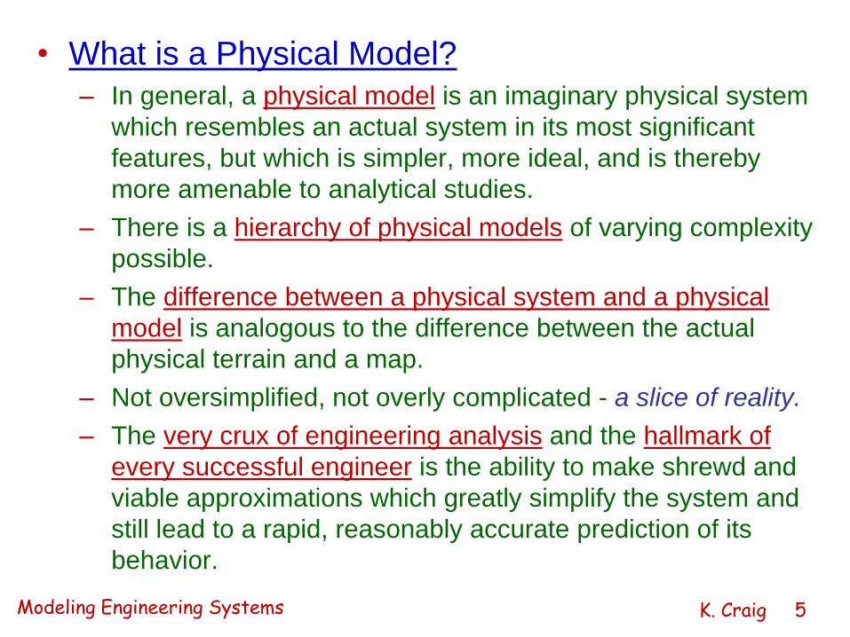
• What is a Physical Model?

– In general, a physical model is an imaginary physical system

which resembles an actual system in its most significant

features, but which is simpler, more ideal, and is thereby

more amenable to analytical studies.

– There is a hierarchy of physical models of varying complexity

possible.

– The difference between a physical system and a physical

model is analogous to the difference between the actual

physical terrain and a map.

– Not oversimplified, not overly complicated - a slice of reality.

– The very crux of engineering analysis and the hallmark of

every successful engineer is the ability to make shrewd and

viable approximations which greatly simplify the system and

still lead to a rapid, reasonably accurate prediction of its

behavior.


• What is a Mathematical Model?

– We apply the Laws of Nature to the Physical Model,

NOT to the Physical System, to obtain the

Mathematical Model.

– What Laws of Nature?

• Newton’s Laws of Motion

• Maxwell’s Equations of Electromagnetism

• Laws of Thermodynamics

– Once we have the Mathematical Model of the

Physical Model, we then solve the equations, either

analytically or numerically, or both to get the greatest

insight, to predict how the Physical Model behaves.

This predicted behavior must then be compared to

the actual measured behavior of the Physical System.


Nonlinear Principle of Superposition

Does Not ApplyNonlinear Differential

Equations

Linear Principle of Superposition

AppliesLinear Differential

Equations

Distributed Dependent Variables are

Functions of Space & TimePartial Differential

Equations

Lumped Dependent Variables are

Functions Only of TimeOrdinary Differential

Equations

Time-Varying Model Parameters Vary in

TimeEquations with Time-

Varying Parameters

Stationary Model Parameters are

Constant in TimeEquations with

Constant Parameters

Continuous Dependent Variables defined

over Continuous Range of

Independent Variables

Differential Equations

Discrete Dependent Variables defined

only for Distinct Values of

Independent Variables

Time-Difference

Equations

Classification of System Models


Ideal Linear System Elements


Balance: The Key to Success

Computer Simulation Without Experimental Verification

Is At Best Questionable, And At Worst Useless!


Balance in Engineering is the Key!

• The essential characteristic of an engineer and

the key to success is a balance between the

following sets of skills:

– modeling (physical and mathematical), analysis

(closed-form and numerical simulation), and control

design (analog and digital) of dynamic physical

systems

– experimental validation of models and analysis and

understanding the key issues in hardware

implementation of designs


• Dynamic Physical System

– Any collection of interacting elements for which there

are cause-and-effect relationships among the time-

dependent variables. The present output of the system

depends on past inputs.

• Analysis of the Dynamic Behavior of Physical

Systems

– Cornerstone of modern technology

– More than any other field links the engineering

disciplines

• Purpose of a Dynamic System Investigation

– Understand & predict the dynamic behavior of a system

– Modify and/or control the system, if necessary


• Essential Features of the Study of Dynamic

Systems

– Deals with entire operating machines and

processes rather than just isolated components.

– Treats dynamic behavior of mechanical, electrical,

electromechanical, fluid, thermal, chemical, and

mixed systems.

– Emphasizes the behavioral similarity between

systems that differ physically and develops general

analysis and design tools useful for all kinds of

physical systems.

– Sacrifices detail in component descriptions so as to

enable understanding of the behavior of complex

systems made from many components.


– Uses methods which accommodate component

descriptions in terms of experimental

measurements, when accurate theory is lacking or

is not cost-effective, and develops universal lab

test methods for characterizing component

behavior.

– Serves as a unifying foundation for many practical

application areas, e.g., vibrations, measurement

systems, control systems, acoustics, vehicle

dynamics, etc.

– Offers a wide variety of computer software to

implement its methods of analysis and design.


Electro-Dynamic Vibration Exciter

Physical System vs. Physical Model


• This "moving coil" type of device converts an electrical

command signal into a mechanical force and/or motion and

is very common, e.g., vibration shakers, loudspeakers,

linear motors for positioning heads on computer disk

memories, and optical mirror scanners.

• In all these cases, a current-carrying coil is located in a

steady magnetic field provided by permanent magnets in

small devices and electrically-excited wound coils in large

ones.

• Two electromechanical effects are observed in such

configurations:

– Generator Effect: Motion of the coil through the magnetic field

causes a voltage proportional to velocity to be induced into the coil.

– Motor Effect: Passage of current through the coil causes it to

experience a magnetic force proportional to the current.


• Flexure Kf is an intentional soft spring (stiff, however, in

the radial direction) that serves to guide the axial motion

of the coil and table.

• Flexure damping Bf is usually intentional, fairly strong,

and obtained by laminated construction of the flexure

spring, using layers of metal, elastomer, plastic, and so

on.

• The coupling of the coil to the shaker table would ideally

be rigid so that magnetic force is transmitted undistorted

to the mechanical load. Thus Kt (generally large) and Bt

(quite small) represent parasitic effects rather than

intentional spring and damper elements.

• R and L are the total circuit resistance and inductance,

including contributions from both the shaker coil and the

amplifier output circuit.


t t f t f t t c t t c t

c c t c t t c t

i c

M x K x B x B (x x ) K (x x )

M x B (x x ) K (x x ) Ki

Li e Ri Kx

Equations

of Motion

f t f t t tt t

t t t tt t

ic c

t t t tc c

c c c c c

0 1 0 0 0

0K K B B K Bx x0

M M M M 0x x

0 0 0 1 0 0ex x

K B K B 0Kx x

M M M M M 1i i

LK R0 0 0

L L

State-Space

Representation

Mathematical Modeling: Laws of Nature applied to Physical Model


Analytical Frequency Response Plots

-100

-80

-60

-40

-20

0

20

Magnitu

de (

dB

)

100

101

102

103

104

105

106

107

90

180

270

360

450

540

Phase (

deg)

Bode Diagram

Frequency (rad/sec)

Typical

Parameter

Values

(SI Units)

L = 0.0012

R = 3.0

K = 190

Kt = 8.16E8

Bt = 3850

Kf = 6.3E5

Bf = 1120

Mc = 1.815

Mt = 6.12

resonance due to flexures

parasitic resonance

due to coil-table

coupling


Experimental Frequency Response Plot

B&K

PM Vibration Exciter

Type 4809


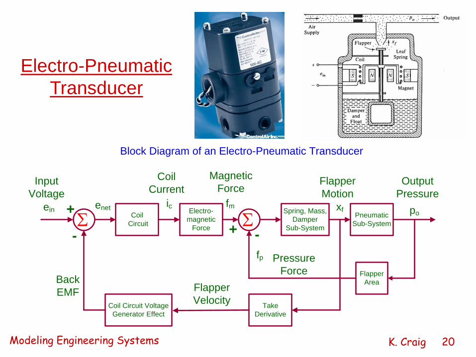
Electro-Pneumatic

Transducer

Coil

Circuit

Electro-

magnetic

Force

+

- + -

Spring, Mass,

Damper

Sub-System

Pneumatic

Sub-System

Flapper

Area

Take

Derivative

Coil Circuit Voltage

Generator Effect

einenet

Back

EMF Flapper

Velocity

ic fm

fp

xf po

Output

Pressure

Flapper

Motion

Pressure

Force

Magnetic

ForceCoil

CurrentInput

Voltage

Block Diagram of an Electro-Pneumatic Transducer


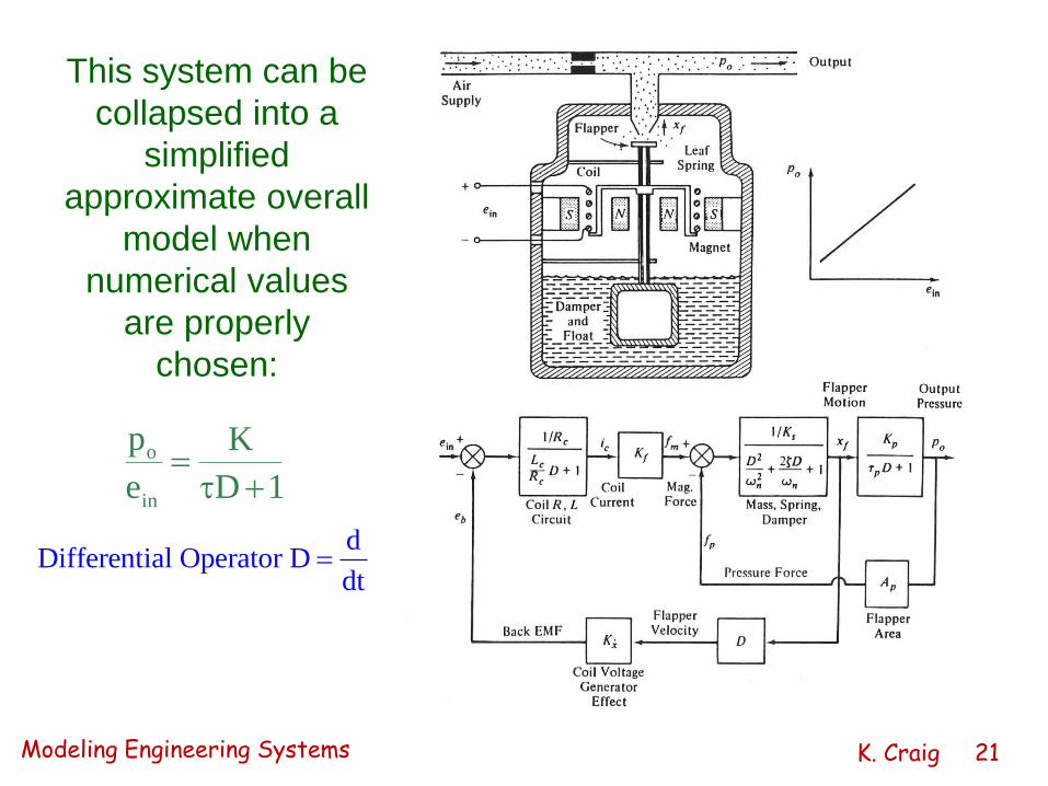
This system can be

collapsed into a

simplified

approximate overall

model when

numerical values

are properly

chosen:

o

in

p K

e D 1

dDifferential Operator D

dt


• It is interesting to note here that while the block

diagram shows one input for the system, i.e.,

command voltage ein , there are possible undesired

inputs that must also be considered.

• For example, the ambient temperature will affect the

electric coil resistance, the permanent magnet

strength, the leaf-spring stiffness, the damper-oil

viscosity, the air density, and the dimensions of the

mechanical parts. All these changes will affect the

system output pressure po in some way, and the

cumulative effects may not be negligible.


Temperature Feedback

Control System:

A Larger-Scale

Engineering System

Bridge

CircuitAmplifier

+

-

Controller

Electro-

Pneumatic

Transducer

ValveChemical

Process

Thermistor

RV

eE

RC

Desired

Temperature

(set with RV)

Block Diagram of an Temperature Control System

Actual

Temperature

(measured with

RC)

eM pM xVTC


• Note that in the block diagram of this system, the

detailed operation of the electropneumatic transducer

is not made apparent; only its overall input/output

relation is included.

• The designer of the temperature feedback-control

dynamic system would consider the electropneumatic

transducer an off-the-shelf component with certain

desirable operating characteristics.

• The methods of system dynamics are used by both

the electropneumatic transducer designer and the

designer of the larger temperature feedback-control

system.


Physical Modeling

Less Real, Less Complex, More Easily Solved

Truth Model Design Model

More Real, More Complex, Less Easily Solved

Hierarchy Of Models

Always Ask: Why Am I Modeling?


• Physical System

– Define the physical system to be studied, along with

the system boundaries, input variables, and output

variables.

• Physical System to Physical Model

– In general, a physical model is an imaginary physical

system which resembles an actual system in its

salient features, but which is simpler, more ideal, and

is thereby more amenable to analytical studies.

There is a hierarchy of physical models of varying

complexity possible.

– Not oversimplified, not overly complicated - a slice of

reality.


– The astuteness with which approximations are

made at the onset of an investigation is the very

crux of engineering analysis.

– The ability to make shrewd and viable

approximations which greatly simplify the system

and still lead to a rapid, reasonably accurate

prediction of its behavior is the hallmark of every

successful engineer.

– What is the purpose of the model? Develop a set

of performance specifications for the model based

on the specific purpose of the model. What

features must be included? How accurately do

they need to be represented?


– The challenges to physical modeling are formidable:

• Dynamic behavior of many physical processes is

complex.

• Cause and effect relationships are not easily

discernible.

• Many important variables are not readily identified.

• Interactions among the variables are hard to

capture.

• Engineering Judgment is the Key!


– In modeling dynamic systems, we consider matter

and energy as being continuously, though not

necessarily uniformly, distributed over the space

within the system boundaries.

– This is the macroscopic or continuum point of view.

We consider the system variables as quantities which

change continuously from point to point in the system

as well as with time and this always leads to a

distributed-parameter physical model which results in

a partial differential equation mathematical model.

– Models in this most general form behave most like the

real systems at the macroscopic level.


– Because of the mathematical complexity of these

models, engineers find it necessary and desirable to

work with less exact models in many cases.

– Simpler models which concentrate matter and energy

into discrete lumps are called lumped-parameter

physical models and lead to ordinary differential

equation mathematical models.

– An understanding of the difference between

distributed-parameter and lumped-parameter models

is vital to the intelligent formulation and use of lumped

models.

– The time-variation of the system parameters can be

random or deterministic, and if deterministic, variable

or constant.


• Comments on Truth Model vs. Design Model

– In modeling dynamic systems, we use engineering

judgment and simplifying assumptions to develop a

physical model. The complexity of the physical model

depends on the particular need, and the intelligent

use of simple physical models requires that we have

some understanding of what we are missing when we

choose the simpler model over the more complex

model.

– The truth model is the model that includes all the

known relevant characteristics of the real system.

This model is often too complicated for use in

engineering design, but is most useful in verifying

design changes or control designs prior to hardware

implementation.


– The design model captures the important features

of the process for which a control system is to be

designed or design iterations are to be performed,

but omits the details which you believe are not

significant.

– In practice, you may need a hierarchy of models of

varying complexity:

• A very detailed truth model for final

performance evaluation before hardware

implementation

• Several less complex truth models for use in

evaluating particular effects

• One or more design models


Approximation Mathematical

Simplification

Neglect small effects Reduces the number and

complexity of the equations of

motion

Assume the environment is

independent of system motions

Reduces the number and

complexity of the equations of

motion

Replace distributed

characteristics with appropriate

lumped elements

Leads to ordinary (rather than

partial) differential equations

Assume linear relationships Makes equations linear; allows

superposition of solutions

Assume constant parameters Leads to constant coefficients in

the differential equations

Neglect uncertainty and noise Avoids statistical treatment


• Neglect Small Effects

– Small effects are neglected on a relative basis. In

analyzing the motion of an airplane, we are unlikely to

consider the effects of solar pressure, the earth's

magnetic field, or gravity gradient. To ignore these

effects in a space vehicle problem would lead to

grossly incorrect results!

• Independent Environment

– In analyzing the vibration of an instrument panel in a

vehicle, we assume that the vehicle motion is

independent of the motion of the instrument panel.


• Lumped Characteristics

– In a lumped-parameter model, system dependent

variables are assumed uniform over finite regions of

space rather than over infinitesimal elements, as in a

distributed-parameter model. Time is the only

independent variable and the mathematical model is

an ordinary differential equation.

– In a distributed-parameter model, time and spatial

variables are independent variables and the

mathematical model is a partial differential equation.

– Note that elements in a lumped-parameter model do

not necessarily correspond to separate physical parts

of the actual system.


– A long electrical transmission line has resistance,

inductance, and capacitance distributed continuously

along its length. These distributed properties are

approximated by lumped elements at discrete points

along the line.

– It is important to note that a lumped-parameter model,

which may be valid in low-frequency operations, may

not be valid at higher frequencies, since the neglected

property of distributed parameters may become

important. For example, the mass of a spring may be

neglected in low-frequency operations, but it becomes

an important property of the system at high

frequencies.


• Linear Relationships

– Nearly all physical elements or systems are inherently

nonlinear if there are no restrictions at all placed on

the allowable values of the inputs, e.g., saturation,

dead-zone, square-law nonlinearities.

– If the values of the inputs are confined to a sufficiently

small range, the original nonlinear model of the

system may often be replaced by a linear model

whose response closely approximates that of the

nonlinear model.

– When a linear equation has been solved once, the

solution is general, holding for all magnitudes of

motion.


– Linear systems also satisfy conditions for

superposition.

– The superposition property states that for a system

initially at rest with zero energy: (1) multiplying the

inputs by any constant multiplies the outputs by the

same constant, and (2) the response to several inputs

applied simultaneously is the sum of the individual

responses to each input applied separately.

• Constant Parameters

– Time-varying systems are ones whose characteristics

change with time.

– Physical problems are simplified by the adoption of a

model in which all the physical parameters are

constant.


• Neglect Uncertainty and Noise

– In real systems we are uncertain, in varying degrees,

about values of parameters, about measurements,

and about expected inputs and disturbances.

Disturbances contain random inputs, called noise,

which can influence system behavior.

– It is common to neglect such uncertainties and noise

and proceed as if all quantities have definite values

that are known precisely.


• Summary

– The most realistic physical model of a dynamic

system leads to differential equations of motion that

are:

• nonlinear, partial differential equations with time-

varying and space-varying parameters

• These equations are the most difficult to solve.

– The simplifying assumptions discussed lead to a

physical model of a dynamic system that is less

realistic and to equations of motion that are:

• linear, ordinary differential equations with constant

coefficients

• These equations are easier to solve and design

with.


Classes of Systems


Pure and Ideal Elements vs. Real Devices

• A pure element refers to an element (spring, damper,

inertia, resistor, capacitor, inductor, etc.) which has only the

named attribute.

• For example, a pure spring element has no inertia or friction

and is thus a mathematical model (approximation), not a

real device.

• The term ideal, as applied to elements, means linear, that

is, the input/output relationship of the element is linear, or

straight-line. The output is perfectly proportional to the

input.

• A device can be pure without being ideal and ideal without

being pure.


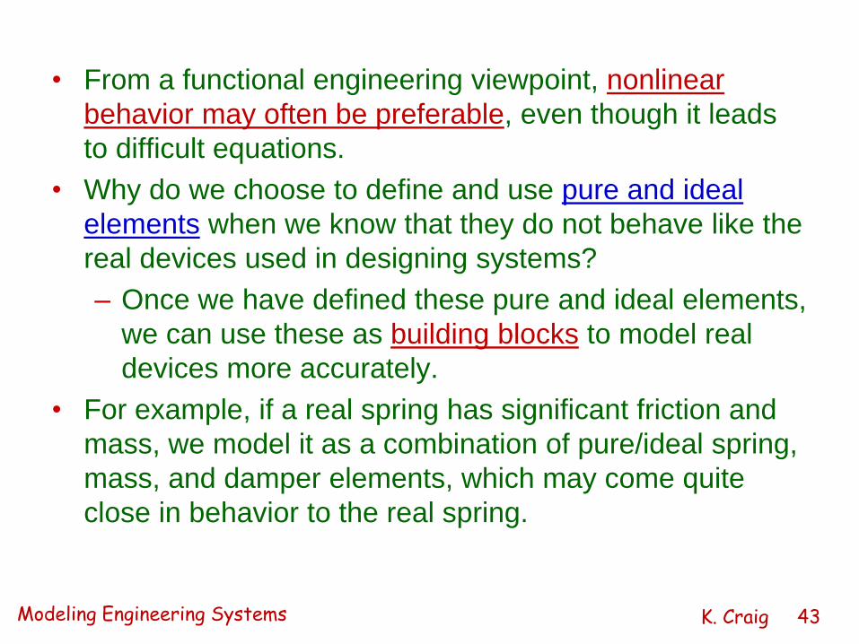
• From a functional engineering viewpoint, nonlinear

behavior may often be preferable, even though it leads

to difficult equations.

• Why do we choose to define and use pure and ideal

elements when we know that they do not behave like the

real devices used in designing systems?

– Once we have defined these pure and ideal elements,

we can use these as building blocks to model real

devices more accurately.

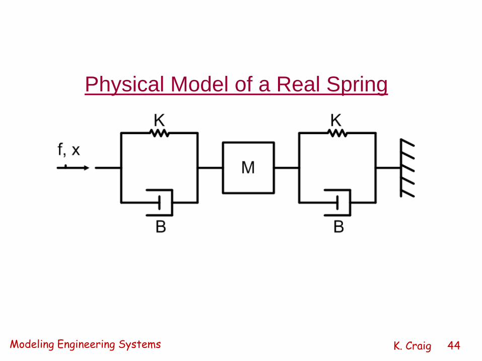
• For example, if a real spring has significant friction and

mass, we model it as a combination of pure/ideal spring,

mass, and damper elements, which may come quite

close in behavior to the real spring.


Physical Model of a Real Spring


• There are three basic types of building blocks,

two that can store energy and one that

dissipates energy.

– All Mechanical Systems have three attributes - mass,

springiness, and energy dissipation. The basic

elements corresponding to these attributes are inertia

(mass), damper (friction), and spring (compliance).

– All Electrical Systems have three attributes -

inductance, resistance, and capacitance. The

corresponding basic elements are inductor, resistor,

and capacitor.


Mechanical System Elements

• It is hard to imagine any engineering system that does

not have mechanical components.

• Motion and force are concepts used to describe the

behavior of engineering systems that employ mechanical

components.

• The three basic mechanical building block elements are:

– Spring (elasticity or compliance) element

– Damper (friction or energy dissipation) element

– Mass (inertia) element

• There are both translational and rotational versions of

these basic building blocks.


• These are passive (non-energy producing) devices.

• Driving Inputs are force and motion sources which cause

elements to respond.

• Each of the elements has one of two possible energy

behaviors:

– stores all the energy supplied to it

– dissipates all energy into heat by some kind of

“frictional” effect

• Spring stores energy as potential energy.

• Mass stores energy as kinetic energy.

• Damper dissipates energy into heat.

• The Dynamic Response of each element is important.


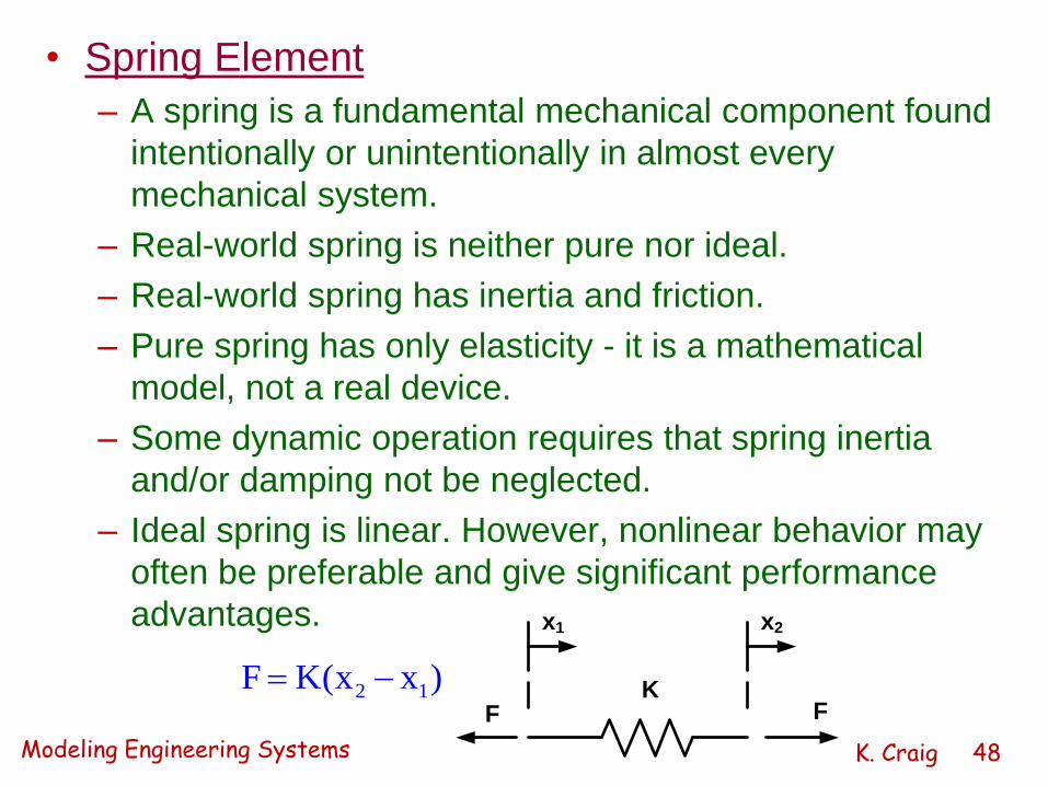
• Spring Element

– A spring is a fundamental mechanical component found

intentionally or unintentionally in almost every

mechanical system.

– Real-world spring is neither pure nor ideal.

– Real-world spring has inertia and friction.

– Pure spring has only elasticity - it is a mathematical

model, not a real device.

– Some dynamic operation requires that spring inertia

and/or damping not be neglected.

– Ideal spring is linear. However, nonlinear behavior may

often be preferable and give significant performance

advantages.

FF

x1 x2

K2 1F K(x x )


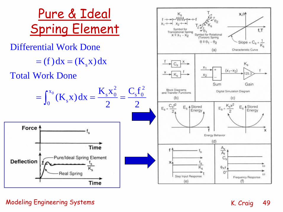
0

s

2 2x

s 0 s 0s

0

Differential Work Done

(f )dx (K x)dx

Total Work Done

K x C f (K x)dx

2 2

Pure & IdealSpring Element


• Damping Element

– A damper is a mechanical component often found in

engineering systems.

– A pure damper dissipates all the energy supplied to it,

i.e., converts the mechanical energy to thermal

energy.

– Various physical mechanisms, usually associated

with some form of friction, can provide this dissipative

action, e.g.,

• Coulomb (dry friction) damping

• Material (solid) damping

• Viscous (fluid) damping


– Shown is a typical mechanical viscous damper. If the

mass and springiness of the piston and cylinder are

small, then the force will be a function of the relative

velocity between the piston and the cylinder.

– Forces on the two ends of the damper are exactly

equal and opposite at all times (just like a spring);

pure springs and dampers have no mass or inertia.

This is NOT true for real springs and dampers.

B

FF

v1 v2

2 1F B(v v )


Pure & IdealDamper Element

Step Input

Force

causes instantly

(a pure damper

has no inertia) a

Step of dx/dt

and a

Ramp of x


• Mass or Inertia Element

– All real mechanical components used in engineering

systems have mass.

– A designer rarely inserts a component for the purpose

of adding inertia; the mass or inertia element often

represents an undesirable effect which is unavoidable

since all materials have mass.

– There are some applications in which mass itself

serves a useful function, e.g., flywheels – a flywheel

is an energy-storage device and can be used as a

means of smoothing out speed fluctuations in engines

or other machines.


– Newton’s Law defines the behavior of mass elements

and refers basically to an idealized “point mass”:

– The concept of rigid body is introduced to deal with

practical situations. For pure translatory motion,

every point in a rigid body has identical motion.

– Real physical bodies never display ideal rigid

behavior when being accelerated.

– The pure and ideal inertia element is a model, not a

real object. Real inertias may be impure (have some

springiness and friction) but are very close to ideal.

forces (mass)(acceleration)

MF

a

F Ma


Pure & IdealInertia Element

Real inertias may be

impure (have some

springiness and friction) but

are very close to ideal.

2 2

x 1 1(D) (D)

f MD T JD

Inertia Element stores energy

as kinetic energy:

2 2Mv J or

2 2


Cantilever Beam

Inertia, Energy Dissipation, Compliance – Does it have these attributes?

Can you model this real device using the pure and ideal building blocks?


Ideal vs. Real Sources

• External driving agencies are physical quantities which

pass from the environment, through the interface into the

system, and cause the system to respond.

• In practical situations, there may be interactions between

the environment and the system; however, we often use

the concept of ideal source.

• An ideal source (force, motion, voltage, current, etc.) is

totally unaffected by being coupled to the system it is

driving.

• For example, a “real” 6-volt battery will not supply 6 volts

to a circuit! The circuit will draw some current from the

battery and the battery’s voltage will drop.


Physical Model to Mathematical Model

• We derive a mathematical model to represent the physical

model, i.e., apply the Laws of Nature to the physical model and

write down the differential equations of motion.

• The goal is a generalized treatment of dynamic systems,

including mechanical, electrical, electromechanical, fluid,

thermal, chemical, and mixed systems.

– Define System: Boundary, Inputs, Outputs

– Define Variables: Through and Across Variables

– Write System Relations: Dynamic Equilibrium Relations and

Compatibility Relations

– Write Constitutive Relations: Physical Relations for Each

Element

– Combine: Generate State Equations


• Define System

– A system must be defined before equilibrium and/or

compatibility relations can be written.

– Unless physical boundaries of a system are clearly

specified, any equilibrium and/or compatibility

relations we may write are meaningless.

• Define Variables

– Physical Variables

• Select precise physical variables (velocity, voltage,

pressure, flow rate, etc.) with which to describe the

instantaneous state of a system, and in terms of

which to study its behavior.


– Through Variables

• Through variables (one-point variables) measure the

transmission of something through an element, e.g.,

– electric current through a resistor

– fluid flow through a duct

– force through a spring

– Across Variables

• Across variables (two-point) variables measure a

difference in state between the ends of an element,

e.g.,

– voltage drop across a resistor

– pressure drop between the ends of a duct

– difference in velocity between the ends of a

damper


– In addition to through and across variables, integrated

through variables (e.g., momentum) and integrated

across variables (e.g., displacement) are important.

• Write System Relations

– Dynamic Equilibrium Relations

• Write dynamic equilibrium relations to describe the

balance - of forces, of flow rates, of energy - which

must exist for the system and its subsystems.

• Equilibrium relations are always relations among

through variables, e.g.,

– Kirchhoff’s Current Law (at an electrical node)

– continuity of fluid flow

– equilibrium of forces meeting at a point


– Compatibility Relations

• Write system compatibility relations to describe

how motions of the system elements are

interrelated because of the way they are

interconnected.

• These are inter-element or system relations.

• Compatibility relations are always relations among

across variables, e.g.,

– Kirchhoff’s Voltage Law around a circuit

– pressure drop across all the interconnected

stages of a fluid system

– geometric compatibility in a mechanical system


• Write Physical Relations for Each Element

– These relations are called constitutive physical

relations as they concern only individual elements or

constituents of the system.

– They are natural physical laws which the individual

elements of the system obey, e.g.,

• mechanical relations between force and motion

• electrical relations between current and voltage

• electromechanical relations between force and

magnetic field

• thermodynamic relations between temperature,

pressure, etc.


– They are relations between through and across

variables of each individual physical element.

– They may be algebraic, differential, integral, linear or

nonlinear, constant or time-varying.

– They are purely empirical relations observed by

experiment and not deduced from any basic

principles.

• Combine System Relations and Physical

Relations to Generate System Differential

Equations


• Study Dynamic Behavior

– Study the dynamic behavior of the mathematical

model by solving the differential equations of

motion either through mathematical analysis or

computer simulation.

– Dynamic behavior is a consequence of the system

structure - don’t blame the input!

– Seek a relationship between physical model

structure and behavior.

– Develop insight into system behavior.


• Comparison: Actual vs. Predicted

– Compare the predicted dynamic behavior to the

measured dynamic behavior from tests on the actual

physical system; make physical model corrections, if

necessary.

• Make Design Decisions

– Make design decisions so that the system will behave

as desired:

• modify the system (e.g., change the physical

parameters of the system, add a sensor, change

the actuator or its location)

• control the system (e.g., augment the system,

typically by adding a dynamic system called a

compensator or controller)

Modeling Engineering Systems Engineer Computer … · Modeling Engineering Systems K. Craig 1 ......

Documents

Transcript of Modeling Engineering Systems Engineer Computer … · Modeling Engineering Systems K. Craig 1 ......