Policy, Research, and External Affairs

WORKING PAPERS

Women In Development

Populatio,l and Human ResourcesDepartment

The World BankAugust 1990

WPS 469

Modeling EconomicBehavior

in Peru's InformalUrban Retail Sector

J. Barry Smithand

Morton Stelcner

Small family businesses that operate outside the formal systemcomprise a large part of the economy in developing countries andmore than half the Peruvian street vendors are women. Thismodel of informal activity in Peru's urban areas elicits policyrecommendations to improve productivity (especially women's)in the informal sector.

Thw Policy,Research. and Extemal Affairs Complex distributes PRE Working Papers todisseminatethe findings of work in progress andto encourage the exchange of ideas among Bank staff and all others interested in development issues. These papers canry the names ofthe authors, reflect only their views, and should he used and cited accordingly. The findings, interpretations, and conclusions are theauthors' own. They should not be attributed to the World Bank, its Board of Directors. its management, or any of its member countries.

Pub

lic D

iscl

osur

e A

utho

rized

Pub

lic D

iscl

osur

e A

utho

rized

Pub

lic D

iscl

osur

e A

utho

rized

Pub

lic D

iscl

osur

e A

utho

rized

Pub

lic D

iscl

osur

e A

utho

rized

Pub

lic D

iscl

osur

e A

utho

rized

Pub

lic D

iscl

osur

e A

utho

rized

Pub

lic D

iscl

osur

e A

utho

rized

LPolicy, Research, and External Affairs

Women In Development |

WPS 469

This paper - a product of the Women in Development Division, Population and lHuman ResourcesDepartment is part of a larger effort in PRE to determine if and how women's productivity (and thusfamily welfare) are improved when women are given more access to education, extension, training, credit,health care, and otherpublic resources. Copies are available free from the Wor!d Bank, 1818 H Street NW,Washington DC 20433. Please contact Maria Abundo, room S9-123, extension 36820 (87 pages withdiagrams and tables).

The informal sector is a collection of loosely Smith and Stelcner analyze Peru's urbanorganized, small-scale competitive family informal sector- particulary women's role in itbusinesses that rely little on nonfamily hired - based on a theoretical model of informal retaillabor, use labor-intensive technologies, and trade (the dominant nonfarm family enterprises),operate largely outside of the legal, bureaucratic, using data from the Peru Living Standardsand regulatory framework in terms of licenses, Survey (PLSS).taxes, and contractual obligations.

They address these questions: What factorsIn Lima, Peru, the informal sector makes up explain differences in the performance of retail

half the labor force, accounts for 61 percent of businesses? If these can be identified, what typesthe hours worked, and generates an astounding of policy initiatives might improve the perfor-39 percent of GDP. More than half the street mance of firms, especially those run by women?vendors are women. Among their recommendations:

In the informal sector, the free play of * Channeling crcdit to small businesses.market forces determiines returns to productivefactors, especially labor. Informal enterprises are * Promoting cooperatives and self-helpconcentrated in low-income areas of urban associations, which provide credit, facilitate bulkcenters, but rural households in Kenya and Peru, purchases, and establish markets for entrepre-among other countries, have joined. neurs.

The informal sector is an important - if not * Providing technical assistance, such asthe sole -- income opportunity for growing short-term instruction in basic management.numbers of the poor. International aid agencieshave explored policies to make informal busi- * Making it easier and cheaper to get businessnesses more profitable. But this surge of interest licenses.is not based on much empirical evidence aboutwhat determines the firms' performance. Nor is * Provide or facilitate cooperative childcarethe value of women's entrepreneurial activities centers, facilities for preparing food, and neigh-reflected in the national accounts. borhood facilities for basic health care to reduce

the heavy workload typical for women.

The PRE Working Paper Series disseminates the findings of work undcr way in the Bank's Policy, Rcsearch. and ExtemalAffairs Complex. Anobjective of thcseries is to get these findings outquickly, even if prescntations are less than fully polished.The findings, interpretations, and conclusions in these papers do not necessarily represent official Bank policy.

Produced by the PRE Dissemination Center

Table of Contents

page

1. Introduction ......................................... 1

2. Some Stylized Facts on the Informal Sector .... ....... 4

2.1 Magnitudes and other Characteristics .... ........ 42.2 The Role of Women ............................... 8

3. Model Formulation and Concepts ........................ 12

3.1 Assumptions ..................................... 133.2 Specific Aspects of the Model ................... 153.3 The Revenue Function of the Firm .... ............ 183.4 Marginal Revenue Products and Profit

Maximization .................................... 19

4. Description of the Data and Variables .... ............. 22

5. The Empirical Model ................................... 28

5.1 Initial Specification ........................... 295.2 Preliminary Tests for Aggregation and Pooling .... 295.3 Diagnostic Analysis ............................. 315.4 Analysis of Nonlinearity ........................ 345.5 Distribution of the Errors ...................... 37

6. Empirical Findings and Interpretation .... ............. 38

6.1 Factor Productivities ........................... 426.2 Nonparametric Evidence .......................... 596.3 Simulation Experiments .......................... 67

7. Policy Implications ................................... 70

7.1 Enterprise-Specific Policies .................... 717.2 Women-Specific Policies .72

Appendix A: Nonparametric Analysis .74Nonparametric Modeling .74Defining Conditional Means and Their Properties 75Estimating Conditional Means and Derivatives .76

Appendix B: The Rural Model .78

Bibliography .84

J. Barry Smith is a member of the Department of Economics, York University, Toronto, Ontario and Morton Stelcneris in the Department of Economics, Concordia University, Montreal, Quebec.

The authors thank the foLlowing individuals: Jorge Castillo, Shahid Khandker, Valerie Kozel, and Marcia Schafgansof the World Bank; Richard Laferriere, Department of Economics, Concordia University; Georges Monette, Department ofMathematics, York University; Jeffrey Racine, Department of Economics, York University; Gwenn B. Hughes, Policy andStrategic Analysis Branch, Labour Canada, Ottawa, and Gail A. Spence, Canadian Pacific Forest Products Limited,Montreal. The authors also benefited from the opportunity to present an earlier version of the paper at a seminarsponsored by the Women in Development Division. Jeffrey Racine performed the nonparametric analysis and wrote AppendixA. The research was funded by the Women in Development Division, the World Bank.

Modeling Economic Behavior in

the Informal Urban Retail Sector of Peru

J. Barry Smith and Morton Stelcner

1. Introduction

Few topics in the literature on development economics have inspired as much

interest, controversy, and rhetoric as the informal sector in developing

countries.1 Here the term is intended as a shorthand expression to describe the

collection oJf loosely organized (but not necessarily fly-by-night) small-scale

competitive family businesses. Such businesses rely little on nonfamily hired

labor. Their technologies are labor intensive and they operate largely outside

the legal, bureaucratic, and regulatory framework reg.rding such matters as

licenses, taxes, and contractual obligations. An important characteristic of the

informal sector is that the free play of market forces generally determines

returns to productive factors, especially labor. The enterprises are usually

concentrated in low-income areas of large metropolitan centers, but it is not

uncommon to find rural households, for example in Kenya and Peru, that have

joined the informal sector.2

There appears to be a consensus that the informal economy is a sizable and

growing component of developing economies. It accounts for a substantial fraction

1 For more recent literature see Bromley (1978), Cornia (1987), Hallak andCaillods (1982), Hart (1987), House (1984), IDB (1987a), Mattera (1985), Moserand Marsie-Hazen (1984), Sethuraman (1981), Stewart (1987), and Tokman (1978).

2 For a discussion see Stelcner and Moock (1988), Moock, Musgrove, andStelcner (1989), and Freeman and Norcliffe (1985).

1

of the labor force, especially in urban areas, and provides an important -- if

not the sole - - income opportunity for growing numbers of the poor. But the

debate about its role in economic development continues. There is considerable

disagreement aoout whether measures should be taken to promote informal

activities as an impetus to economic growth and a strategy for improving the

earnings of low-income households.

The place of the informal sector in development is all the more imnortant

because of the severe economic crisis in most third world economies. As Cornia

(1987) discusses, households faced with sharply reduced employment and incom3

prospects in the formal (or modern) sectors -- manufacturing, services, mining,

and government - - tend to seek employment and income opportunities in the

informal economy. The first to shift are those who have lost jobs in the formal

sector. Next, employed formal sector workers, especially government employees,

resort to moonlighting activities, most of which are informal. As household

incomes decline, married women and children who previously did not work in the

market are drawn into informal market activities, and soon new entrants to the

labor force begin to find jobs in the informal rather than the formal sector. 3

The rapid growth of the informal sector has led international aid agencies

and governments to explore policies to improve the profitability of such

businesses. This surge of interest, however, is not based on much empirical

evidence about the underlying determinants of the performance of the firms.

Informals perform a remarkable array of activities, ranging from vending

foodstuffs and prepared foods to consumer goods and services, including

3 Several recent studies have identified these general patterns. See Cornia(1987), IDB (1987b), PREALC (1985), van der Gaag, Stelcner and Vijverberg (1989),and Tokman (1986).

2

carpentry, tailoring, barbering, shoe-repair, domestic work, vehicle and tool

repairs, and transport. In addition, small-scale entrepreneurs manufa re

textiles, garments, footwear, household utensils, musical instruments, metal

products, furniture and wood products, and leather goods. They process foods

and beverages, and recycle junk. Some firms are also involved in such illicit

ventures as smuggling and processing alcohol and cocaine.

This research analyzes the informal sector in Peru, particularly the role

of women, based on a theoretical model of informal retail trade that uses data

from the Peru Living Standards Survey (PLSS). Retailing is the domirnant nonfarm

family enterprise. The central questions are: What factors explain differences

in the performance of retail businesses? Assuming that these cc.nsiderations can

be identified, what types of policy initiatives might improve the performance

of firms, particularly those run by women? The analysis is confined to urban

areas where most of these bus.nesses are located . 4

4We attempted to provide an analysis of nonfarm enterprises in both urban andrural areas. But the limited size of the sample in rural areas precluded theestimation of a mod-l that we were confident of using. The resu- ts for ruralareas are in appendix L.

3

2. Some Stylized Facts on the Informal Sector

2.1 Magnitudes and Other Characteristics

Informal economic activity is a mainstay of the Peruvian economy. Its

sustained growth stands in marked contrast to formal activity, which has

deteriorated in the last decade at an alarmingly rapid rate. There is extensive

evidence that a high proportion of the labor force, especially the Lemale

component, is in informal activities. As Glewwe and de Tray (1989) and Suarez-

Berengue]a (1987) discuss, the majority of the bottom socioeconomic strata in

urban areas earns a livelihood from self-employment in the informal sector.

Peru's shadow economy has recently attracted worldwide attention5 as a

result of the recent publication of El Otro Sendero: La Revolucibn Informal6 by

Hernando de Soto, a businessman and president of Lae Instituto Libertad y

Democracia (ILD) in Lima. He concludes that the informal sector is the dominant

and most dynamic part of the economy, and believes that removing the burdensome

obstacles to legitimacy (such as bureaucratic red tape) would considerably

improve Peru's economic malaise.

Several other recent studies corroborate de Soto's view ,hat a sizable

portion, perhaps a majority, of the labor force is in the informal sector.7

Surveys by the ILD in 1985 and 1986 show that the informal sector in Lima makes

up almost half the labor force, accounts for 61 percent of the hours worked and

s See The Economist, February 18 and September 23, 1989; and Leaders, March 1989(12) 1.

6 The English translation is The Other Path: The Invisible Revolution in theThird World. (See de Soto 1989).

7See Althaus and Morelli (1980), Kafka (1984), Litan and others (1987), Stelcnerand Moock (1988), Moock, Musgrove, and Stelcner (1989), Strassmann (1987),Suarez-Berenguela (1987), Vargas Llosa (1987), Webb (1977), and World Bank(1987).

4

generates an astounding 39 percent of GDP (1984). For such sectors as commerce

mind personal services this share exceeds 60 percent. Litan and others (1987)

report that the official national accounts estimate of the informal sector's

contribution to GDP it, 3'84 resulted in an understatement of total GDP of 23

percent. Perhaps even more striking is the estimate that 439,000 Lima residents

depend on the underground commercial economy, and almost three fourths (314,000)

of these individuals depend on street sales. According to de Soto, these

activities generated about $25 million a month in gross sales in 1985 and an

average ret per capita profit of $58 a month, about 40 percent more than the

legal minimum wage. The 314,000 street merchants include 91,455 street vendors,

are 42 percent of the Lima work force involved in commerce.

The ILD surveys show that women make up 54 percent of the street vendors.

Eighty-six percent of the street merchants occupy curbside sites, while the

remaining 14 percent rove the streets. Business is also conducted in (illegal)

cooperative markets -- collections of kiosks, stalls and booths. Of the 331

markets in Lima, 274 were put up illegally; only 57 were built by the government.

It is estimated that $41 million has been invested in these illegal markets,

which employ about 125,000 people (including sc - 40,000 vendors). More than 80

percent of the street vendors and 64 percent of the informal markets are found

in low-income districts.

According to recent studies that used the Peru Living Standards Survey8,

half of the 5,100 households surveyed owned at least one nonagricultural family

enterprise. Of the 27,000 individuals in the survey, 13,600 were in the labor

force and 97 percent were employed. More than 4,500 worked in nonfarm family

8 See Stelcner and Moock (1988), and Moock, Musgrove, and Stelcner (1989).

5

businesses, and 3,100 worked in family enterprises as their main occupation.

About 6,200 worked on family farms.

Metropolitan Lima accounted for 34 percent of n3nfarm family businesses,

other urban areas for 44 percent, and rural areas only 22 percenc.. Of course,

a large fraction of rural households also operate farms. These proportions

correspond closely to the distribution of family workers and households across

regions. The average number of enterprises per household is 1.25.

These family businesses are dominated by retail trade, manufacturing

(especially textiles), and personal services (mainly in urban areas). Retail

trade encompasses small shops, inns and cafes, kiosks, stalls, and street

vending. Nontextile manufacturing includes food, beverages, pottery, furniture,

toys,novelties, and musical instruments. The textile sector includes spinning,

weaving, and tailoring. Personal services range from laundries and hairdresser.

and barbers to entertainment, auto and electrical repairs, and cleaning

services. Most businesses rely on just one or two family workers; the use of

hired labor is negligible.

Many firms do not own any capital or inventory and often have no operating

expenses. In the retail sector selling is often on consignment or commission.

Large factories, wholesalers, and stores in the formal sector often provide the

goods and perhaps the cart, stall, or kiosk. The goods are sold either on

straight commission, or on consignment: the sellers pay only for what they sell

and return the unsold goods. Factories often subcontract textile, clothing,

leather and footwear manufacturing to family enterprises, which they provide with

materials and equipment. In the labor-intensive personal services sector, little

use is made of capital equipment. Thus it is not surprising that many family

6

businesses in the dominant sectors reported little or no capital, inventories,

or operating expenses.

How much credit do informals use and obtain? The Peru Living Standards

Survey provided information on the current debt position of each household, and

on the source and termns of loans obtained in the past year.

Only 10 percent of the households that operated businesses reported that

they received loans or were in debt. This is not surprising for several reasons.

First, the PLSS was conducted when inflation rates were extremely high (June

1985-July 1986). (During the first half of 1985 the annual inflation was 200

percent, and in the first half of 1986 monthly inflation was 4 to 5 percent.

Such high rates of inflation are unlikely to foster a willingness to lend, except

at interest rates so high that few households would choose to borrow. Second,

given a sensitivity to questions about indebtedness, the Peru Living Standards

Survey probably underestimated the debt among respondents. (To preserve good

will, questions on debt and credit were last in a long questionnaire". Third,

given the uncertain legal position of family businesses, their ability to obtain

credit from formal lending institutions is very restricted at best. As Carbonetto

(1984), Mescher (1985), and Kafka (1984) document, only a minute fraction of

informal sector firms in Lima borrow from financial intermediaries in the formal

sector. Households that need to borrow must depend on loan sharks and

pawnbrokers, or resort to a "pandeiro". This is a revolving fund to which

members make a weekly contribution. A lottery determines the winner of the week's

contributions .9

9 See Mescher(1985), World Bank (1989).

7

In Lima, retail trade, personal services, and manufacturing account for

more thati 80 percent of the businesses and almost 85 percenc of the family

workers (Table 1). The single most important activity is retail trade. The

pattern is the same in the rest of Peru. In other urban areas the proportions

are 86 percent (retail trade, 52 percent) and 90 percent. In rural areas 80

percent of entrepreneurial families and workers are in retail trade (43 percent)

or manufacturing, particularly textiles. These are typical informal sector

endeavors in most developing countries. What distinguishes Peru from other

countries is the unusually large proportion of women and households in these

activities.

2.2 The Role of Women

The Peru Living Standards Survey shows that women dominate the informal

economy. Schafgans (1989) notes t'at women make up about 45 percent of the labor

force. The vast majority work in family-owned firms and farms. Table 2 shows that

82 percent of the 5,952 employed women worked in family-owned nonfarm businesses

(28 percent) or on family farms (54 percent). The remaining 18 percent were wage

earners, mostly in urban areas. In Lima 45 percent of employed women were wage

earners in contrast to 19 percent in other urban areas. In rural areas only 5

percent of employed women worked as salaried employees, usually as school-

teachers and clerks in the public sector. There is practically no labor market

for women in rural areas. In Lima, 38 percent of the women were employed in

nonfarm businesses and 17 percent in agricultural activities; in other urban

areas the corresponding proportions were 44 and 37 percent, and in rural areas

11 and 84 percent.

8

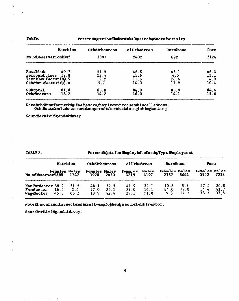
TabTh. Percendfbgttribuf5 forbEhitysineAqtctofictivity

Metrbima OthdirbaAreas AlUrbabreas RuraUreas Peru

No.oWDbservationlO45 1387 2432 692 3124

Retdilade 40.7 51.5 46.8 43.1 46.0Persofekvices 19.8 12.4 15.6 4.5 13.1TextM1mnufacturiI*.9 12.2 11.6 26.4 14.9Othd4anufacturidrW.4 9.7 10.0 11.9 10.4

Subtotal 81.8 85.8 84.0 85.9 84.4Othdefctors 18.2 14.2 16.0 14.1 15.6

Note0thdfanufactubtraidoedbvera6irxii rcorduebis cel1laiieems .OthLactdcswlud6nstruc inanporbdtmdi i:adhnintishfrnhunting.

SourcberIiiviSgandaSldviey.

TABLE 2. Percentfbtribuflmpfoy&dbo]Pordvfrypefmployment

Metrbima OthdfrbaAreas AlUrbaAreas Rurareas Peru

Females Males Females Males Females Males Females Males Females MalesNo.o9Dbservatl8fll 1747 1978 2450 3215 4197 2737 3041 5952 7238

NonFarSector 38.2 31.5 44.1 32.5 41.9 32.1 10.6 5.3 27.5 20.8Farigector 16.5 3.4 37.0 25.1 29.0 16.1 84.0 77.0 54.4 41.7Wageector 45.3 65.1 18.9 42.4 29.1 51.8 5.3 17.7 18.1 37.5

Notefhemonfaumfarwectae£melf-employhowgsectDf etirdAbor.

SourcBerhiviigandaSdBvey.

9

Of the 7,238 employed men surveyed, 21 percent worked in nonfarm

enterprises and 42 percent worked on family farms, while 38 percent worked as

wage employees (65 percent in Lima. 42 percent in other urban areas, and 18

percent in rural areas). In Lima about 32 percent of employed men worked in

family businesses and 3 percent on farms, while in other urban areas the

proportions were 33 and 25 percent, respectively. In rural areas only 5 percent

of men worked in nonfarm family businesses; 77 percent worked on family farms.

In the retail food and textile sectors women account for three-fourths of

the family workers. In retail nonfood and food processing sectors they make up

60 to '0 percrnt of the work force, and account for about half the workers in

urban personal services. The remaining family businesses -- transportation,

construction, wood and4 chemical manufacturing, wholesale trade, hunting and

fishing, and professional services -- are dominated by men and employ only a

small fraction of women. There appears to be a clear division of labor between

men and women. The proportion of women employed in the formal sector is much

smaller than that of men and the informal sector activities that women pursue

are considerably different from those of men.

The role of women in familv enterprises is also highlighted by the large

proportion of family businesses in the dominant three sectors that employ

exclusively women and children under 20. In urban and rural areas about half the

family retail businesses rely only on women and children. About 40 percent of

that provide services firms employ only women and children. In textiles, which

are largely home-based, oner 66 percent of the rural concerns employ only women

and children. In Lima the proportion rises to 70 percent and in other urban areas

to 75 percent. These data suggest that women not only make up a high proportion

of family workers but also operate the family businesses.

10

Despite their importance in these businesses, the value of women's

entrepreneurial activities is not adequately reflected -- if at all -- in the

national accounts. There have been very few attempts to assess their contribution

to the economy or to analyze the relative performance of men and women in the

informal economy. This is particularly true in Peru and other Latin American

countries where such work has gone largely unnoticed, with the possible exception

of domestic work.

Moreover, official Latin America data'° do not give accurate information

about women's economic activities. Most of the empirical economic research on

family businesses has focused on agricultural activities or on the activities

of self-employed urban men. Agricultural research tends to ignore informal

nonfarm economic activities in rural areas. And most of the research on the self-

employed analyzes individuals rather than the enterprise, ignoring the

contributions to income of capital, nonlabor inputs, and the labor of women and

children. These last are typically excluded because most surveys report them as

unpaid family workers, while men are usually reported as paid family workers

(Chiswick 1983).11

This analysis focuses on the family business rather than the self-employed

individual, thereby incorporating enterprise characteristics -- capital,

location, nonlabor inputs -- and the labor of all family workers.1 2

10 See Recchine de Lates and Wainerman 1986; Bunster and Chaney 1985; Babb 1984.

11 Often it is not clear whether these self-employed earnings refer to the valueof gross sales or to the value of net production, that is, sales less cost ofmaterials and other inputs.

12 For related approaches see Blau (1985), Chiswick (1983), Strassmann (1987),Vijverberg (1988), and Teilhet-Waldorf and Waldorf (1983).

11

3. Model Formulation and Concepts

The analysis of the model of the revenue process of retail enterprises

includes a theoretical characterization of revenue generation by retailers as

well as a basis for estimating economic magnitudes (such as productivity). The

model incorporates three features of sales revenue -- price, potential customers,

and the process by which a potential customer becomes a purchaser, at a given

price.

The traditional economic model of production is extended to explain the

production process of firms that expend resources in selling as well as in

producing goods or services. For example, consider a street vendor who sells

pencils at a given price at a busy intersection. An important consideration

involves measuring the vendor's output. To argue that output can be measured in

terms of the number or constant dollar value of transactions (in this case,

pencils sold) is akin to measuring output by the value of inputs, and misses a

vital feature of the retailing process. That is, in every attempt (whether

successful or not) to convince a passerby to purchase a pencil, the vendor is

also making a sales effort, that includes information about the product and its

availability. To measure output by the volume or value of transactions measures

only that part of the vendor's activity that is successful.

In our model we argue that an enterprise in the retail sector effectively

'produces' the probability that a contacted customer will make a purchase. We

argue further that the firm can adjust its inputs (including labor, capital,

materials, and inventory) to change the likelihood that it will make a sale.

Changing inputs may range from increasing inventories to providing more

information to customers.

12

The model is not explicitly one of profit maximization and not necessarily

one where optimization leads to a dual relationship between cost and production.

The data (particularly on prices) are not sufficient to estimate such a model.

More important, it is not clear whether the textbook model of cost-efficient

production and profit maximization is a useful hypothesis. It may be more

reasonable to assume simply that firms make efficient use of their inputs and

then to test whether observed decisions are consistent with profit maximization.

Since our goal is to provide an empirical model of production for retail firms,

in our discussion of the theoretical model we will also refer to problems and

limitations in the applied work.

3.1 Assumptions

Assume that potential shoppers arrive randomly at the location of a

vendor. Thus the contacts between buyers and sellers is a random variable. The

average number of such contacts will depend upon the characteristics of the firm,

including its location and reputation. 13 There is no guarantee that a shopper

arriving at an enterprise will decide to make a purchase. Of two seemingly

identical shoppers, one may decide to buy while the other does not, independently

of the characteristics of the enterprise. The fraction of shoppers that makes

a purchase is thus a random variable.

We assume that at each point in time and for a given price and type of

good, a customer has a random yet rationally determined threshold response level

to the vendor's sales effort. Suppose shopper j has threshold level ti. The

decision by the customer whether or not to make the purchase involves a

comparison of t. with the variable T. defined as tbh index of sales effort

13 No information is available concerning repeat buyers or customers who purchasemore than one unit of a good.

13

produced by firm i. If TL > tj, then the arriving customer will buy from firm i.

If customers have their threshold levels ti distributed according to the same

(distribution) function F, then a firm with sales effort T. will make a sale to

a randomly arriving customer with probability F(Td). This probability, F(T1), can

also be thought of as the fraction of arriving customers that buy from the firm.

Part of the firms' decision making involves setting the level of TL.

The model described above is similar to stochastic choice models that

have lately become quite popular in labor economics. By analogy, the decision

to buy is like the decision to enter the labor force and the condition that tj

< TL is similar to the requirement that the reservation wage at zero work is less

than the market wage.

The enterprise can change its operating characteristics to affect the

fraction of shoppers that makes a purchase. For example, a business can increase

its inventory or stay open longer. Such factors are considered productive if

increasing them raises the fraction of potential consumers who make purchases

or, equivalently, increases the probability that a given shopper will make a

purchase. Since the fraction of shoppers who buy is bounded from above by unity,

in the limit for large quantities of factors there must be zero returns at the

margin to increasing the level of productive factors. Similarly, while

enterprises may adopt different mixes of factors (perhaps due to financing

restrictions), labor is a common feature; no retail firm can operate without

labor. The fraction of shoppers making purchases will approach zero as the amount

of labor input approaches zero. This need not be true, however, for such inputs

as capital (for example, a cart or stall) or inventory. Without these factors

a customer can still make a purchase. The model is not constrained ex ante to

require profit maximizing decisions on the part of firms. We do, however, examine

14

whether the properties of the estimated model are consistent with profit

maximization.

In applied work, neither the total number of units sold nor the selling

price per unit are generally known. Data sets typically do not contain this

information. Similarly, information on the number of customer contacts and the

fraction of shoppers who buy is not available. At most, information on revenues,

costs, and other characteristics of factors employed by the firm will be

available in cross-section or time series data sets. With cross-section data the

absence of separate information on price and quantity may cause fewer problems

than in a time series setting where constancy of price is difficult to justify

as a working assun,ption.

3.2 Specific Aspects of the Model

The expected price per unit received by an enterprise is defined as p8.

It is assumed that agents treat pB as independent of the decisions of individual

enterprises and of customers.

The expected number of shoppers arriving at enterprise i is defined as

NE(Xi). NE is assumed to depend upon (a vector of) characteristics of firm i, X',

one element of which, for example, would be location. Differences in the expected

number of arrivals at firm i versus firm j are assumed to depend only on

differences in the characteristics of vectors xL and x3. Because the total number

of arrivals is subject to random effects, firm i will not in general observe

arrivals equal to N1(XI). In the applied work of subsequent sections it is

assumed that the expected number of arrivals to firm i can be expressed as:

nN

NE(XL) - exp[a0 + E a xi] (1)

Thus,nN

lnNE(XL) ao + E axi (2)J=1 .2 .1

15

where XLJ is a measure of the jth characteristic in firm i. The specification of

NE(Xt ) is seen to be linear in its logarithm and introduces the ex ante

restriction that the number of arrivals is nonnegative.

The fraction of shoppers that make a purchase or, equivalently, the

probability that firm i makes a sale to a randomly arriving customer, is given

by F(T(Z')). F depends upon a vector of firm i's characteristics, ZI, which

includes labor, materials/expenses, capital, and inventories.

In keeping with the discussion of the previous section, F can be written

as a function of T1 where T. is an index of sales effort and output produced by

firm i and given by:

TL = T(Zi) (3)

F will be a nondecreasing function of TL, bounded from below by 0 and from

above by 1. Indeed, F is just the cumulative distribution function for the random

variable t representing individual consumer purchasing thresholds. A drawing of

t for a given customer j (tj) shows the level of (an index of) sales effort

needed to guarantee that individual j will make a purchase.

By adopting the above characterization of retailing, we obtain a model

whereby something can be produced (sales effort or the probability of a purchase)

with no guarantee that any consumer will make a purchase or that a firm will be

observed to make a transaction. This will occur when the level of (the index of)

sales effort produced by a given firm falls short of the threshold level

necessary to convince the customer to buy. In the applied research it is assumed

16

that the cumulative distribution function, F, is given by the logistic

function. 14

F(TL) 11 + exp[-T] (4)

From (3) it will be recalled that the index TL is a function of a vector

of characteristics ZL of firm i. This function must reflect the fact that labor

is indispensable to the activity but that other factors are not. If we define

ZL as the labor component of Z', the indispensability of labor can be introduced

by requiring T, to be an increasing function of the logarithm of z1L. Introducing

the remaining factors affecting TL in a linear fashion leads to the

specification:nF

TL- bo + bllnzL + E b zL (5)1 J-2 j J

where nF is the number of factors used in the production of T.. Given that b, >

0, labor will be an indispensable factor with a positive marginal product in

terms of increasing the index T.. As labor becomes small, TL decreases without

bound and F(T1) approaches zero. Any other factor zi will be productive as long

as bi > 0. The parameter bo is the value of the index when labor is equal to one

unit and all other factors are zero.It is reasonable to expect bo to be negative

and large enough in absoltte value such that exp[-b.] is large and F(TL), the

average frequency of sales, is small when almost no factors are allocated to

sales.

As a final point, it is possible to extend the production analogy to

consider isoquants which, in this case, are isoprobability contours of F. Since

" This specification of a logistic probability distribution function has provedvaluable in other areas of applied economic research and it has the added benefitthat it leads to applied models that are somewhat easier to estimate than thosebased upon the cumulative normal distribution function.

17

F is a monotone increasing transformation of T., isoquants of T1 will coincide

with isoquants of F. These isoquants will be straight lines for pairs of inputs,

excluding labor. Alternatively, for pairs of inputs one of which is labor

measured on the vertical axis, the isoquants are horizontally parallel and

intersect the vertical axis. Production processes such as this are called quasi-

linear.

3.3 The Revenue Function of the Firm

The discussion contained in the foregoing sections leads to the

specification of a revenue function for a representative firm in the retail

sector. This function is comprised of both a deterministic and a stochastic

component. The expected revenue of firm i, RE5 , is given by the product of the

expected price and the expected number of buyers. The latter quantity is itself

given by the product of the expected number of arriving customers and the

fraction of customers who make purchases. In terms of the notation introduced

above,

RE = pENE(XI)F(T(ZI)) (6)L

We assume that the stochastic influence on revenues enters

multiplicatively. Thus observed revenues of firm i, R., are given by:

RL = R' exp[vL] (7)

where vL is a random variable incorporating uncertainties in the price level and

the unforecastable factors affecting the number of customer contacts with the

firm. We assume that vL is such that E[exp[v,]] = 1. Our applied work will

involve estimating the revenue function in logarithmic form. In terms of the

18

specification of NE and F(T.) in previous sections, the estimating equation will

be of the form:

lnRL - lnpE + ao +F 1 ajx3 - ln(l + exp[-(b. + b,lnz' + 2 bzi')]) + vi (8)

A nonlinear least squares algorithm is used to obtain point estimates of

the parameters of the model. Since independent information on average price is

not available, the coefficient estimate of ao will not identify the parameter ao.

3.4 Marginal Revenue Products and Profit Maximization

The derivative of the expected revenue function with respect to a right-

hand side variable (such as labor or capital) can be interpreted as the expected

marginal revenue product of the variable. In cases where the unit price of the

factor is known, the expected marginal revenue product can be compared with this

magnitude to partially assess the efficiency of the firm. For example, if a firm

is maximizing expected profits, the factor price and the marginal revenue product

should, on average, coincide. In cases where data on factor prices are not

available (a common occurrence in the informal sector), the derivative of the

expected revenue fur -tion can be considered the shadow price of the factor. This

shadow price is the amount of money that would be paid to the factor if the

existing situation represented profit-maximizing behavior. In both situations

the results lead to interesting insights for policy analysis.

The model is quite flexible with respect to possible relationships between

revenue and such productive factors as labor, capital, and expenses. The fact

that F(T1) is strictly bounded from above and below introduces some features into

the relationship between factors that often do not arise in standard models of

19

production. To highlight some of these prope-ties, we present the following

example of an expected revenue function.

Suppose that a simplified expected revenue function with two factors (x

and y) is given by:

R 1/(1 + exp[a - x - y]), a 2 0 (9)

where R is (expected) revenue, price and customer effects are fixed (in this

example) and (a, -1, -1) are the estimated coefficients of the model. The

(expected) marginal revenue product of factor x, R., is the derivative of the

right hand side of (9) with respect to x and is given by:

Rx =R - R2 (10)

The marginal revenue product of x will be positive as long as the right

hand side of (10) is positive. Given the definition of R in (9), this will always

be the case because R < 1.

The response of the marginal revenue product function to changes, ceteris

paribus, in x and y is important for determining the suitability of any profit

maximization hypothesis and for determining the relationships between productive

factors. The slope of the marginal revenue product function is given by the

derivative of the right hand side of (10) with respect to x. Denoting this slope

by R., differentiation yields:

R.. - R,(1 - 2R) (11)

Eventually, the marginal revenue product curve will slope downwards as R

becomes larger than .5. There may be a range of x values where the marginal

revenue product curve is upward sloping. This would be the case, for example,

20

if when x - 0, the value of the expression (a - y) exceeds 0 (and hence, R < .5

when x 0). Thus the slope of the marginal revenue product curve tor x depends

in part on the quantity of the other productive factors. Within a profit

maximization setting, the marginal revenue product curves must be downward

sloping if the optimality conditions are to be satisfied.

It was noted above that the levels of other factors affect the slope of

the marginal revenue product curve for a given factor. The position of the

marginal revenue product curve for a given factor is influenced by the quantities

of the other factors as well. This effect can be illustrated by considering the

change in the marginal revenue product of x as y changes. Denoting this effect

by R.., the right hand side of (10) can be differentiated with respect to y to

obtain:

R' = cRY1 - 2R) (R - R2)(1 - 2R) (12)

where R. is the marginal revenue product of y. Thus in this simple example, as

long as R < .5, increasing y makes x more productive. Eventually, though, as y

becomes increasingly large, more of the factor y will exert a negative effect

on the (marginal) productivity of x. The explanation lies in the fact that the

probability of making a sale (in this case 1/(1 + -n[I - x - y]) is bounded

from above by 1. The only way this condition can be met for increasing values

of y and fixed x is if both factors are made less productive. If this were not

to happen then x could be increased over a feasible range of values and the

probability could be made greater than 1.

21

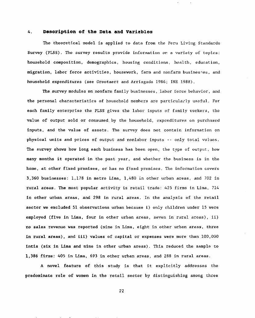
4. Description of the Data and Variables

The theoretical model is applied to data from the Peru Living Standards

Survey (PLSS). The survey results provide informiiation or. a variety of topics:

household composition, demographics, housing conditions, health, education,

migration, labor force activities, housework, farm and nonfarm busines-es, and

household expenditures (see Grootaert and Arrlagada 1986; INE 1988).

The survey modules on nonfarm family businesses, labor force behavior, and

the personal characteristics of household members are particularly useful. For

each family enterprise the PLSS gives the labor inputs of family workers, the

value of output sold or consumed. by the household, expenditures on purchased

inputs, and the value of assets. The survey does not contain information on

physical units and prices of output and nonlabor inputs -- only total values.

The survey shows how long each business has been open, the type of output, how

many months it operated in the past year, and whether the business is in the

home, at other fixed premises, or has no fixed premises. The information covers

3,360 businesses: 1,178 in metro Lima, 1,480 in other urban areas, and 702 in

rural areas. The most popular activity is retail trade: 425 firms in Lima, 714

in other urban areas, and 298 in rural areas. In the analysis of the retail

sector we excluded 51 observations urban because i) only children under 15 were

employed (five in Lima, four in other urban areas, seven in rural areas), ii)

no sales revenue was reported (nine in Lima, eight in other urban areas, three

in rural areas), and iii) values of capital or expenses were more than 100,000

intis (six in Lima and nine in other urban areas). This reduced the sample to

1,386 firms: 405 in Lima, 693 in other urban areas, and 288 in rural areas.

A novel feature of this study is that it explicitly addresses the

predominate role of women in the retail sector by distinguishing among three

22

types of businesses: 1) female.-only firms (possibly with children), 2) male-only

firms (perhaps with children), and 3) mixed firms. Most retail firms employ only

one or two family workers and do not use hired laborers. (See Table 3)

We use the follr.wing variables in the empirical analysis. The dependent

variable is the logarithm of monthly gross revenues, which is the value of

output. The set of regressors can be grouped into two categories -- those that

describe customer arrivals and those chat affect the probability of a purchase.

The former group includes the age of the enterprise in years, which can be

interpreted as a reflection of the reputation of the firm and perhaps as a

predictor of learning by doing in attracting clientq. Also included is the place

of operation as a proxy for ease of access by customers. Two dummy variables -

- 'in the home' and 'at a fixed location' (a kiosk or stall) -- incorporate the

site information. Itinerant operations with no fixed location (such as peddling

and street hawking) are excluded.

The following variables are deemed to affect the probability of a

purchase. First, the value of capital, which includes land, buildings, furniture,

tools, machinery, equipment and vehicles. Second, the value of inventory stocks

and third, monthly operating expenses which measure the cost of goods purchased

for resale, raw materials, and such items as repairs, utilities, and fuel. The

timeframe of this variable corresponds to that of the dependent variable. The

fourth variable is labor input, measured by the logarithm of monthly hours

devoted by all family workers in the ent._rprise. The annual hours of farming

labor are divided by the months of operation. Other aspects of managerial or

sales skills are described by two proxies: 1) total work experience (in years)

of the most experienced adult family worker in the firm and 2) the level of

educational attainment of the most educated adult family worker in the firm. Work

23

experience is entered with linear and quadratic (scaled by 100) terms. The

effects of educational attainment are entered in two alternative ways. First,

we use three dummy variables - primary school completed, secondary school

completed, and postsecondary school completed; the excluded category is less than

primary schoolirg. Second, we use three splines - years of primary school (zero

to five), secondary school (six to ten) and postsecondary school (more than 10

years). Finally, the effects of vocational training are reflected by a dummy

variable that takes a value of unity if any adult family worker in the enterprise

had vocational training, or a value of zero otherwise.

24

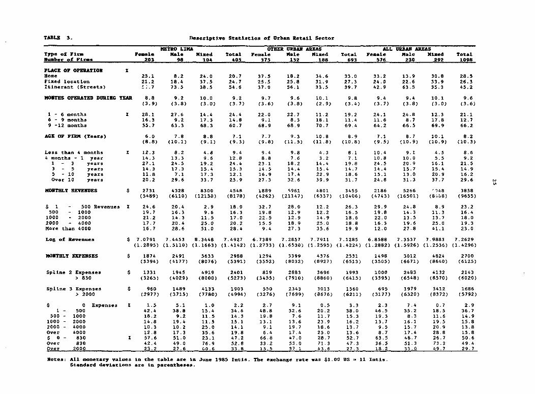
TABLE 3. Pescriptjte Statistics of Urban Retail Sector

METRO LIMA OTHER URBAN ARFAS ALL URBAN AREASType of Firm Female Male Mixed Total Female Male Mixed Total Female male mixed TotalRumber of Firms 203 98 104 405 375 132 188 693 576 230 292 1098

PLACE OF OPERATION SHome 25.1 8.2 24.0 20.7 37.5 18.2 34.6 33.0 33.2 13.9 30.8 28.5Fixed location 21.2 18.4 37.5 24.7 25.5 25.8 31.9 27.3 24.0 22.6 33.9 26.3Itinerant (Streets) ''.7 73.5 38.5 54.6 37.0 56.1 33.5 39.7 42.9 63.5 35.3 45.2

MONTHS OPERATED DURING YEAR 8.8 9.2 10.0 9.2 9.7 9.6 10.1 9.8 9.4 9.4 10.1 9.6(3.9) (3.8) (3.0) (3.7) (3.6) (3.8) (2.9) (3.4) (3.7) (3.8) (3.0) (3.6)

1 - 6 months X 28.1 27.6 14.4 24.4 22.0 22.7 11.2 19.2 24.1 24.8 12.3 21.16 - 9 months 16.3 9.2 17.3 14.8 9.1 8.3 18.1 11.4 11.6 8.7 17.8 12.79 -12 months 55.7 63.3 68.3 60.7 68.9 68.9 70.7 69.4 64.2 66.5 69.9 66.2

AGE OF FIRM (Tears) 6.0 7.8 8.8 7.1 7.7 9.3 10.8 8.9 7.1 8.7 10.1 8.2(8.8) (10.1) (9.1) (9.3) (9.8) (11.5) (11.8) (10.8) (9.5) (10.9) (10.9) (10.3)

Less than 4 months Z 12.3 8.2 4.8 9.4 9.4 9.8 4.3 8.1 10.4 9.1 4.5 8.64 months - 1 year 14.3 13.3 9.6 12.8 8.8 7.6 3.2 7.1 10.8 10.0 5.5 9.21 - 3 years 27.1 24.5 19.2 24.4 23.1 18.2 14.4 19.8 24.5 20.9 16.1 21.53 - 5 years 14.3 17.3 15.4 15.3 14.5 14.4 15.4 14.7 14.4 15.7 15.4 14.95 - 10 years 11.8 7.1 17.3 12.1 16.9 17.4 22.9 18.6 15.1 13.0 20.9 16.2Over 10 years 20.2 29.6 33.7 25.9 27.3 32.6 39.9 31.7 24.8 31.3 37.7 29.6

MONTHLY REVENUES $ 2731 4328 8300 4548 i8 8 95961 4801 3455 2186 5266 '148 3858

(5489) (6110) (12138) (8178) (4262) (21147) (6337) (10406) (4743) (16501) (8;o&8) (9655)

$ 1 - 500 Revenues X 24.6 20.4 2.9 18.0 32.7 28.0 12.2 26.3 29.9 24.8 8.9 23.2500 - 1000 19.7 16.3 9.6 16.3 19.8 12.9 12.2 16.5 19.8 14.3 11.3 16.41000 - 2000 21.2 14.3 11.5 17.0 22.5 12.9 14.9 18.6 22.0 13.5 13.7 18.02000 - 4000 17.7 20.4 25.0 20.2 15.5 18.9 25.0 18.8 16.3 19.6 25.0 19.3More than 4000 16.7 28.6 51.0 28.4 9.4 27.3 35.6 19.9 12.0 27.8 41.1 23.0

Log of Revenues S 7.0791 7.4453 8.3448 7.4927 6.7389 7.2857 7.7911 7.1285 6.8588 7.3537 7.9883 7.2629(1.2895) (1.5110) (1.1663) (1.4142) (1.2733) (1.6530) (1.2595) (1.4224) (1.2882) (1.5926) (1.2536) (1.4296)

MONTHLY EXPENSES $ 1874 2491 5633 2988 1294 3399 4376 2531 1498 3012 4824 2700(3394) (4177) (8076) (5391) (3552) (8032) (8927) (6513) (3505) (6671) (8640) (6125)

Spline 2 Expenses $ 1331 1945 4919 2401 819 2883 3696 1993 1000 2483 4132 2143> 830 (3265) (4029) (8000) (5273) (3455) (7910) (8860) (6415) (3395) (6548) (8570) (6020)

Spline 3 Expenses $ 960 1489 4133 1903 550 2343 3013 1560 695 1979 3412 1686> 2000 (2977) (3715) (7780) (4994) (3276) (7699) (8676) (6211) (3177) (6320) (8372) (5792)

$ 0 Expenses X 1.5 5.1 1.0 2.2 2.7 9.1 0.5 3.3 2.3 7.4 0.7 2.91 - 500 42.4 38.8 15.4 34.6 48.8 32.6 20.2 38.0 46.5 35.2 18.5 36.7

500 - 1000 18.2 9.2 11.5 14.3 19.8 7.6 11.7 15.3 19.3 8.3 11.6 14.91000 - 2000 14.8 19.4 11.5 15.1 13.1 13.6 23.9 16.2 13.7 16.1 19.5 15.82000 - 4000 10.3 10.2 25.0 14.1 9.1 19.7 18.6 13.7 9.5 15.7 20.9 13.8Over 4000 12.8 17.3 35.6 19.8 6.4 17.4 25.0 13.6 8.7 17.4 28.8 15.8$ 0 - 830 X 57.6 51.0 23.1 47.2 66.8 47.0 28.7 52.7 63.5 48.7 26.7 50.6Over 830 42.4 49.0 76.9 52.8 33.2 53.0 71.3 47.3 36.5 51.3 73.3 49.4Over 2000 23.2 27.6 60.6 33.8 15.5 37.1 43.6 27.3 18.2 33.0 49.7 29.7

Notes: All monetary values in the table are in June 1985 Intis. The exchange rate vas $1.00 US = 11 Intis.Standard deviations are in parentheses.

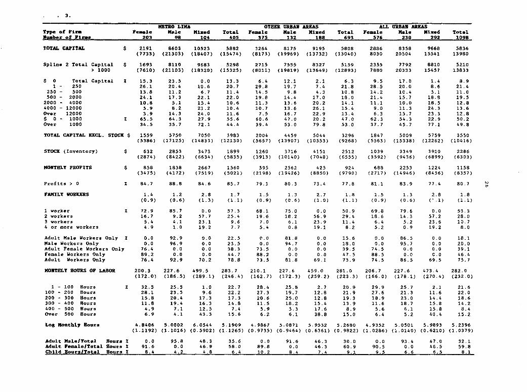
. 3.

METRO LIKA OTHER URBAN AREAS ALL URBAN AREASType of Finr Female Kale Mized Total Female Kale Mixed Total Female Male Mized TotalNumber of Firms 203 98 104 405 375 132 188 693 576 230 292 1098TOTAL CAPITAL $ 2191 8603 10523 5882 3264 8175 9195 5808 2886 8358 9668 5836(7733) (21303) (18407) (15474) (8173) (19969) (13732) (13040) 8030 20504 15541 13980Spline 2 Total Capital $ 1693 8110 9683 5298 2715 7555 8327 5159 2355 7792 8810 5210> 1000 (7610) (21103) (18320) (15325) (8011) (19819) (13649) (12893) 7880 20333 15457 13833

$ 0 Total Capital X 15.3 23.5 0.0 13.3 6.4 12.1 2.1 6.3 9.5 17.0 1.4 8.91 - 250 26.1 20.4 10.6 20.7 29.8 19.7 7.4 21.8 28.5 20.0 8.6 21.4250 - 500 13.8 11.2 6.7 11.4 14.5 9.8 4.3 10.8 14.2 10.4 5.1 11.0500 - 2000 24.1 17.3 22.1 22.0 19.8 14.4 17.0 18.0 21.4 15.7 18.8 19.52000 - 4000 10.8 5.1 15.4 10.6 11.3 13.6 20.2 14.1 11.1 10.0 18.5 12.84000 - 12000 5.9 8.2 21.2 10.4 10.7 13.6 26.1 15.4 9.0 11.3 24.3 13.6Over 12000 3.9 14.3 24.0 11.6 7.5 16.7 22.9 13.4 6.3 15.7 23.3 12.8$ 0 - 1000 2 65.5 64.3 27.9 55.6 60.6 47.0 20.2 47.0 62.3 54.3 22.9 50.2Over 1000 34.5 35.7 72.1 44.4 39.4 53.0 79.8 53.0 37.7 45.7 77.1 49.8

TOTAL CAPITAL EXCL. STOCK $ 1559 5750 7050 3983 2004 4459 5044 3296 1847 5009 5759 3550(5386) (17125) (14833) (12130) (5657) (13907) (10553) (9268) (5563) (15338) (12262) (10416)STOCK (Inventory) $ 632 2853 3473 1899 1260 3716 4151 2512 1039 3349 3910 2286(2874) (8422) (6634) (5835) (3913) (10140) (7048) (6555) (3592) (9436) (6899) (6303)

MONTHLY PROFITS $ 858 1838 2667 1560 595 2562 425 924 688 2253 1224 1158(3475) (4172) (7519) (5021) (2198) (19426) (8850) (9790) (2717) (14946) (8456) (8357)Profits > 0 2 84.7 88.8 84.6 85.7 79.1 80.3 73.4 77.8 81.1 83.9 77.4 80.7

FAMILY WORKERS 1.4 1.2 2.8 1.7 1.5 1.3 2.7 1.8 1.5 1.3 2.8 1.8(0.9) (0.6) (1.3) (1.1) (0.9) (0.6) (1.0) (1.1) (0.9) (0.6) (1.1) (1.1)1 worker % 72.9 85.7 0.0 57.3 68.1 75.0 0.0 50.9 69.8 79.6 0.0 53.32 workers 16.7 9.2 57.7 25.4 19.6 18.2 56.9 29.4 18.6 14.3 57.2 28.03 workers 5.4 4.1 23.1 9.6 7.0 6.1 23.9 11.4 6.4 5.2 23.6 10.74 or more workers 4.9 1.0 19.2 7.7 5.4 0.8 19.1 8.2 5.2 0.9 19.2 8.0

Adult Male Workers Only X 0.0 92.9 0.0 22.5 0.0 81.8 0.0 15.6 0.0 86.5 0.0 18.1Male Workers Only 0.0 96.9 0.0 23.5 0.0 94.7 0.0 18.0 0.0 95.7 0.0 20.0Adult Female Workers Only 76.4 0.0 0.0 38.3 73.5 0.0 0.0 39.5 74.5 0.0 0.0 39.1Female Workers Only 89.2 0.0 0.0 44.7 88.2 0.0 0.0 47.5 88.5 0.0 0.0 46.4Adult Workers Only 76.4 92.9 70.2 78.8 73.5 81.8 69.1 73.9 74.5 86.5 69.5 75.7

MONTHLY HOURS OF LABOR 200.3 227.6 499.5 283.7 210.1 227.6 459.0 281.0 206.7 227.6 473.4 282.0(172.0) (186.5) (289.1) (246.4) (162.7) (172.3) (259.2) (223.3) (166.0) (178.1) (270.4) (232.0)1 - 100 Hours 2 32.5 25.5 1.0 22.7 28.4 25.8 2.7 20.9 29.9 25.7 2.1 21.6100 - 200 Hours 28.1 23.5 9.6 22.2 27.3 19.7 12.8 21.9 27.6 21.3 11.6 22.0200 - 300 Hours 15.8 20.4 17.3 17.3 20.6 25.0 12.8 19.3 18.9 23.0 14.4 18.6300 - 400 Hours 11.8 19.4 16.3 14.8 11.5 18.2 15.4 13.9 11.6 18.7 15.8 14.2400 - 500 Hours 4.9 7.1 12.5 7.4 5.9 5.3 17.6 8.9 5.6 6.1 15.8 8.4Over 500 Hours 6.9 4.1 43.3 15.6 6.2 6.1 38.8 15.0 6.4 5.2 40.4 15.2

Log Monthly Hours 4.8406 5.0002 6.0544 5.1909 4.9867 5.0871 5.9532 5.2680 4.9352 5.0501 5.9893 5.2396(1.1192) (1.1016) (0.5902) (1.1265) (0.9735) (0.9464) (0.6361) (0.9822) (1.0286) (1.0140) (0.6210) (1.0379)

Adult Male/Total Hours 2 0.0 95.8 48.3 35.6 0.0 91.6 46.3 30.0 0.0 93.4 47.0 32.1Adult Female/Total Hours X 91.6 0.0 46.9 58.0 89.8 0.0 46.3 60.9 90.5 0.0 46.5 59.8Child HourslTotal Hours X 8.4 4.2 4.8 6.4 10.2 8.4 7.4 9.1 9.5 6.6 6.5 8.1

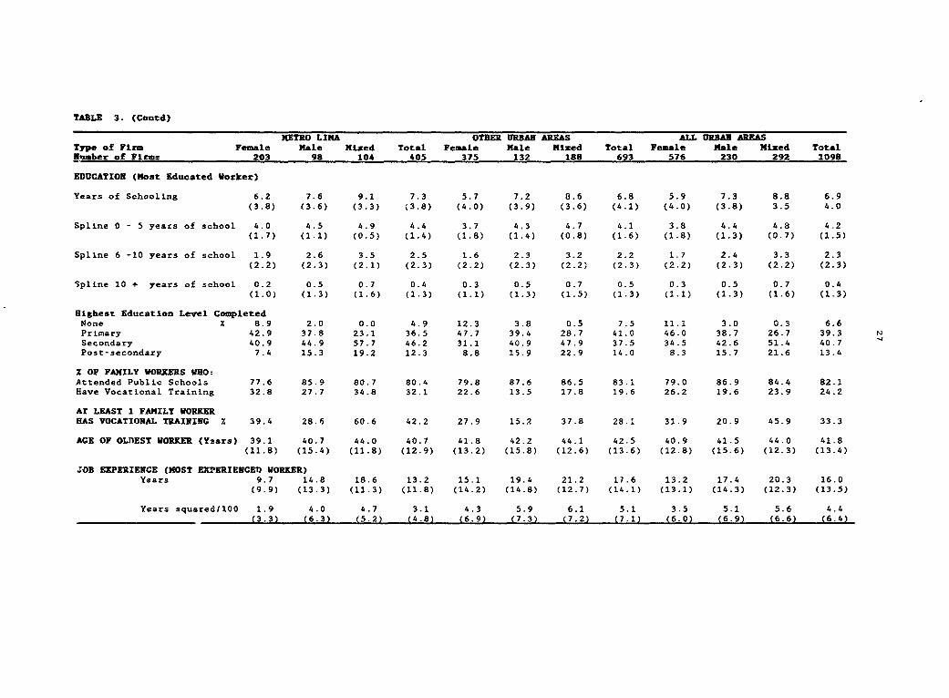
TABLE 3. (Coutd)

METRO LIMA OTE URBAN AREAS ALL URBAN ARRASType of Ftrm Female Male Mixed Total Female Kale Mixed Total Female Male Mixed TotalNumber of Firms 203 98 104 405 375 132 188 693 576 230 292 1098EDUCATION (Most Educated Worker)

Years of Schooling 6.2 7.6 9.1 7.3 5.7 7.2 8.6 6.8 5.9 7.3 8.8 6.9(3.8) (3.6) (3.3) (3.8) (4.0) (3.9) (3.6) (4.1) (4.0) (3.8) 3.5 4.0Spline 0 - 5 years of school 4.0 4.5 4.9 4.4 3.7 4.3 4.7 4.1 3.8 4.4 4.8 4.2(1.7) (1.1) (0.5) (1.4) (1.8) (1.4) (0.8) (1.6) (1.8) (1.3) (0.7) (1.5)Spline 6 -10 years of school 1.9 2.6 3.5 2.5 1.6 2.3 3.2 2.2 1.7 2.4 3.3 2.3(2.2) (2.3) (2.1) (2.3) (2.2) (2.3) (2.2) (2.3) (2.2) (2.3) (2.2) (2.3)Spline 10 + years of school 0.2 0.5 0.7 0.4 0.3 0.5 0.7 0.5 0.3 0.5 0.7 0.4(1.0) (1.3) (1.6) (1.3) (1.1) (1.3) (1.5) (1.3) (1.1) (1.3) (1.6) (1.3)Highest Education Level CompletedNone % 8.9 2.0 0.0 4.9 12.3 3.8 0.5 7.5 11.1 3.0 0.3 6.6Primary 42.9 37.8 23.1 36.5 47.7 39.4 28.7 41.0 46.0 38.7 26.7 39.3Secondary 40.9 44.9 57.7 46.2 31.1 40.9 47.9 37.5 34.5 42.6 51.4 40.7Post-secondary 7.4 15.3 19.2 12.3 8.8 15.9 22.9 14.0 8.3 15.7 21.6 13.4

2 OF FAMILY WORKERS WHO:Attended Public Schools 77.6 85.9 80.7 80.4 79.8 87.6 86.5 83.1 79.0 86.9 84.4 82.1Have Vocational Training 32.8 27.7 34.8 32.1 22.6 13.5 17.8 19.6 26.2 19.6 23.9 24.2Ar LEAST 1 FAMILY WORKERHAS VOCATIONAL TRAINING X 39.4 28.6 60.6 42.2 27.9 15.2 37.8 28.1 31.9 20.9 45.9 33.3AGE OF OLDEST WORKER (Years) 39.1 40.7 44.0 40.7 41.8 42.2 44.1 42.5 40.9 41.5 44.0 41.8(11.8) (15.4) (11.8) (12.9) (13.2) (15.8) (12.6) (13.6) (12.8) (15.6) (12.3) (13.4)JOB EXPERIENCE (MOST EX2ERIENCED WORKER)

Years 9.7 14.8 18.6 13.2 15.1 19.4 21.2 17.6 13.2 17.4 20.3 16.0(9.9) (13.3) (11.3) (11.8) (14.2) (14.8) (12.7) (14.1) (13.1) (14.3) (12.3) (13.5)

Years squared/100 1.9 4.0 4.7 3.1 4.3 5.9 6.1 5.1 3.5 5.1 5.6 4.4(3.3) (6.3) (5.2) (4.8) (6.9) (7.3) (7.2) (7.1) (6.0) (6.9) (6.6) (6.4)

5. The Empirical Model

This section reports the specification and estimation of the revenue model

for the informal retail sector. In contrast to popular approaches to estimating

the properties of production technologies, we introduce no assumptions about the

optimizing behavior of agents. One reason for this is that there are seldom well-

developed markets for the factors employed by these firms and thus no way to

construct independent measures of the opportunity cost necessary for optimizing

models.

Our work uses the revenue function specified in equation (8). Ultimately,

though, the statistical process of specification, estimation, diagnostic

analysis, and nonlinearity analysis that we employ is iterative. In our case

there were iterations with respect to both model specification and

inclusion/exclusion of data points in the sample reflecting the inflow of

information from the battery of diagnostic tests to which the model and data

were subjected. Since our model is nonlinear in some parameters it was necessary

to estimate the extent of this nonlinearity to determine whether the local

diagnostic analysis, based on a version of the model linearized about the least

squares optimum and other measures of goodness of fit and precision, retained

their traditional meaning. It is known, for example, that as the measured degree

of model/parameter nonlinearity increases,traditional confidence ellipsoids may

become distorted, with the result that traditional measures of (joint)

significance of parameters lose their validity.

We describe below the iterations of testing and diagnostic analysis that

separate the initial model from the final model for which parameter estimates

are reported. The approach led to a model that is extremely robust, provides an

excellent fit of the data, and is very close to the initial model in both

28

specification and sample. Two versions of the final model are reported: the

difference between the two lies in the measurement of education -- dummy or

splined variables. Finally, as a further test of validity, we analyzed the data

using nonparametric techniques (see Appendix B). The results are discussed below.

5.1 Initial Specification

The initial model was given by:

lnRL - ao + alLOCTION_HOME + a2LOCATION_FIXED + a3FIRM_AGE - ln(l + e T)

+ VL (13)

where:

TL - bo + bjEXPENSES + b2CAPITAL + b3STOCK + b,ln(LABOR)

+ b5 TRAINING + b6 SCHOOL_PRIMARY + b7 SCHOOL_SECONDARY + b8 SCHOOL_POSTSEC

+ bgEXPERIENCE + b2OEXPERIENCE2 (14)

The model was fitted to three subsamples of the data: Lima, other urban

areas, and rural areas. All the first round point estimates of the parameters

(obtained by a nonlinear least squares Gauss-Newton algorithm) had the correct

signs and between 50 and 60 percent of the variance in the logarithm of revenues

was explained.

5.2 Preliminary Tests for Aggregation and Pooling

The initial results showed similar patterns in the estimated parameters

of the Lima and other urban areas models. Some parameters from the rural model

were similar to their counterparts for Lima and for other urban areas. These

results led to the hypothesis that an aggregate model based on a pooled sample

could be estimated. At the same time it was necessary to determine whether we

were justified in pooling data among female, male, and mixed enterprises. This

question was particularly important given that one of our goals was to estimate

29

women's productivity. Finally, regardless of the outcome of these initial

hypothesis tests, all the tests would have to be redone since the model

specification and the data set might change as a result of information obtained

from the diagnostic analysis (see below). All hypotheses were tested using the

sample likelihood ratio statistic compared with its 1 percent critical value.

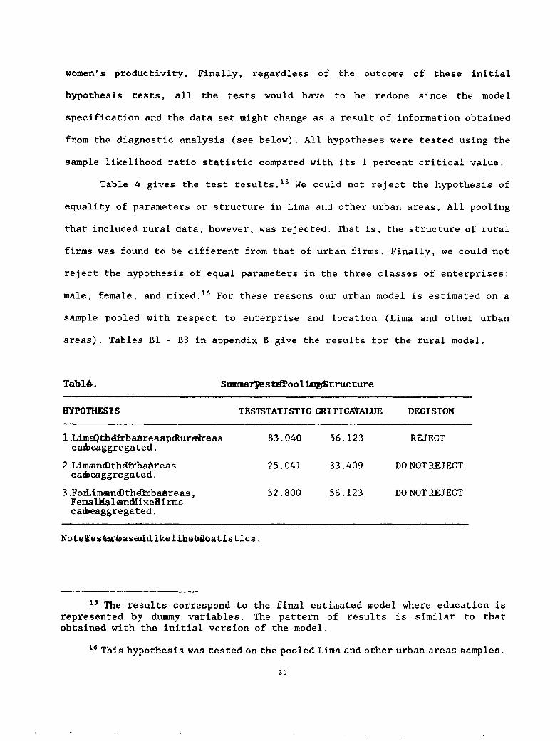
Table 4 gives the test results.'5 We could not reject the hypothesis of

equality of parameters or structure in Lima and other urban areas. All pooling

that included rural data, however, was rejected. That is, the structure of rural

firms was found to be different from that of urban firms. Finally, we could not

reject the hypothesis of equal parameters in the three classes of enterprises:

male, female, and mixed."6 For these reasons our urban model is estimated on a

sample pooled with respect to enterprise and location (Lima and other urban

areas). Tables Bl - B3 in appendix B give the results for the rural model.

Tabl4. Summarqestifool1iagtructure

HYPOTHESIS TESTSTATISTIC CRITICAQALUE DECISION

l.Lima1thdfrbaArea;i&ur %reas 83.040 56.123 REJECTcalbeaggregated.

2.LimaandthdirbaAreas 25.041 33.409 DO NOT REJECTcalbeaggregated.

3.FoiLimandDthd1rbaAreas, 52.800 56.123 DO NOTREJECTFemalftlean&ixegirmscaibeaggregated.

Note.TestwbaseAilikelihabeoatistics.

15 The results correspond to the final estimated model where education is

represented by dummy variables. The pattern of results is similar to that

obtained with the initial version of the model.

16 This hypothesis was tested on the pooled Lima and other urban areas samples.

30

5.3 Diagnostic Analysis

Our analysis involved assessing the sensitivity of parameter estimates

to what we term "data problems." Although the PLSS is an unusually clean data

set, where much effort was devoted to correcting anomalies, it is still open to

a variety of impurities due to, inter alia, measurement errors, data entry, and

inaccurate reporting by respondents and enumerators. Advances in statistical

research have made it possible to implement a set of data diagnostic tests to

reveal statistical problems arising from imperfect data or highly influential

sets of observations. These tests provide another useful way to assess the

reliability of a given model."7

The diagnostic techniques involve searching the data for single

observations or sets of observations that differ significantly from the 'average'

data point and may have an excessive influence on the regression results.

Parameter estimates that are highly dependent on the properties of small

subsamples of the data should be treated with caution. For this reason the

isolation and careful study of influential observations is an important task in

applied modeling. The theory behind these tests for linear models has been

developed extensively in the statistics literature. For our nonlinear model, the

tests were performed on a version of the model linearized about the nonlinear

least squares optimum.

Two possible sources of influential observations are high leverage points

and outliers. A high leverage point is an observation for which the vector of

independent variables is "far" from the rest of the data. In the leverage

analysis, the data were searched for points that were farthest from the center

" For an excellent discussion of these issues, see Belsley, Kuh, and Welsch(1980), and Chatterjee and Hadi (1988).

31

of the remaining data. Since leverage points need not be influential points,

these observations were iteratively dropped and the model reestimated to see if

the points were particularly influential in determining the overall fit. The

second test involved plotting residuals against leverage values to identify

outliers, that is, those observations where the residuals were large. We isolated

observations where the fitted values of the model were farthest from the actual

values of the dependent variables. These observations were removed from the data

set and the model was reestimated to evaluate their influence on the regression

results. This process was repeated several times because the removal cf any one

high leverage point can, and generally does, cause a change in the set of high

leverage points.

Finally, we examined the plots of the studentized residuals against the

independent variables and against the fitted values of the dependent variable.

The first set of plots was studied for patterns (for example, positive residuals

for large values of the variables) that might indicate that the specification

was not robust. The second plots provided information about possible nonlinear

relationships in the residuals.

Ultimately the analysis showed that 15 data points were influential. That

is, their removal from the sample led to significant changes in the parameter

estimates for capital, stock, and expenses. All the influential observations we

isolated had extremely large values for capital, stock, or expenses (more than

100,000 intis). We chose not to include these 15 data points in the estimation

of subsequent models.

In strdying the stability of the estimated parameters, we were

particularly concerned about their sensitivity to restrictions on the capital,

stock, and expenses variables. Our analysis involved setting critical values for

32

these variables and dropping observations in excess of these values. When we

reestimated the model for successively smaller critical values, we found that

the parameters associated with capital, stock, and expenses were quite sensitive

to these restrictions, but that other parameters were stable. The parameter

estimates for capital, stock, and expenses tended to increase as the independent

variables were restricted.

These results suggest that a model with constant coefficients for capital,

stock, and expenses might not be appropriate. The coefficients should be given

the flexibility to decrease as the variables increase.18 The economic

interpretation of these results was that there were variable returns to these

factors beyond what the original specification of the model could encompass.

We reestimated the model with piecewise linear splines for capital, stock,

and expenses. Because the nonlinear nature of the model combined wich the large

sample size made estimation somewhat expensive, we undertook only limited

experimentation on determining the knots of the splines. Up to three segments

appeared necessary to remove a large amount of the instability of the

coefficients.

The parameter instability that remained appeared to involve a trade-off

in the values of the parameters of the stock the capital variables similar to

a multicollinearity problem. Independent of the choice of knot points, the spline

coefficients for the stock variables were never significant and typically had

t-statistics less than 0.5. The estimated coefficients were of the wrong sign

as well. But if the added spline variables for stock were removed, an unstable

18 We also estimated the model with quadratic terms for capital, stock, andexpenses, but the parameter instability remained. Box-Cox transformations werenot possible because these variables often had values of zero.

33

but statistically significant coefficient of the correct sign arose for the

remaining stock variable.

We resolved this problem by aggregating the stock and capital variables

into a single variable called total capital. We reasoned that statistical

testing based on the likelihood ratio test provided no clear evidence against

the aggregation decision. Whether or not the test rejected or did not reject

aggregation depended on the number of spline variables introduced. In no case

was aggregation as strongly rejected as the competing hypothesis that the stock

variable should simply be dropped from the model. Second, the model with capital

and stock aggregated was characterized by stable and significant parameter

estimates of the correct sign. Third, prior to aggregation the nonlinearity tests

(see below) indicated that the model was highly nonlinear in terms of the

curvature properties of the estimated revenue function. After aggregation this

problem disappeared.

5.4 Analysis of Nonlinearity

The diagnostic analysis is based on the assumption that the underlying

regression model is linear in the parameters. Other statistics, such as

confidence intervals about the point estimates of the parameters, assume that

the model is linear. This linearity assumption is violated in the strict sense,

but that there will be a linearized version of the model around the nonlinear

least squares optimum. The important question to raise is whether the linearized

version of the nonlinear model is accurate over a sufficiently large range of

the parameter space so as to include confidence intervals measured in the

standard way. Alternatively, the model may be so nonlinear that the linear

approximation model becomes unacceptably inaccurate within the range of the

traditionally (linearly) measured confidence intervals.

34

Current research in the statistics literature has been aimed at resolving

such questions using differential geometry. This branch of mathematics has well-

developed notions and measures of curvature and nonlinearity. Nonlinearity of

statistical models has beer, reduced, in part, to the study of the radius (of

curvature) of the largest approximating ball "covered" by the estimated model.

Intuitively, the larger the radius of curvature, the better will be the local

linear approximation to the model and the more confident one can feel about

results based on the linearized model. The total curvature of a model can be

decomposed to three parts: one representing the intrinsic curvature of the model

(and about which nothing can be done short of respecification) and the other two

representing parameter effects curvature (which can, to some degree, be mitigated

by reparametrization of the model without distorting the specification).

Statistical tests of the extent of curvature relative to the distance of the

estimated model from the dependent variable can be performed and the significance

of deviations from linearity can be assessed (see Bates and Watts 1980).

Table 5 shows the nonlinearity analysis arising from the last diagnostic

iteration. All the parameters of the model fell within acceptable limits for

nonlinearity. Those parameters for which the curvature measures were greatest

were associated with the spline variables for capital and expenses. These results

confirm our finding that it was inappropriate to specify constant coefficients

for the aggregate expenses and capital variables. They also suggest that the

spline approach leads to a model with a sufficiently accurate linear

approximation around the nonlinear least squares optimum. The nonlinearity

analysis increased our confidence in the quality of the estimated model and in

the validity of applying traditional statistical tests to the model.

35

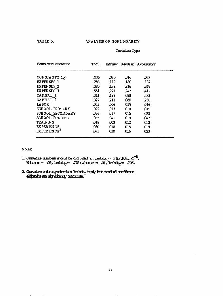
TABLE 5. ANALYSIS OF NONLINEARIrY

CurvaMn Type

Pmn etr C omnskd Tota kltrkis2 GeodC s A oakn

CONSTANT2 .036 .020 .014 .027EXPEN SES_1 .286 .119 .180 .187EXPEN SES_2 .385 .172 .216 ,269EXPENSES_3 551 .271 247 .41'CAPITAL_1 .311 .199 .088 .223CAPIrAL_2 .327 .211 .080 .236LABOR .023 .006 .015 .016SCHOOL_PRHM4ARY .022 .013 .010 .015SCHOOL_SECONDARY .034 .017 .015 .025SCHOOL_POSTSEC .065 .041 .019 .047TRA IN ING .018 .003 .012 .012EX PER IEN CE .030 .018 .015 .019EXPERIENCE2 .041 .030 .016 .023

No':

1. Cu r& nbe riould be onpaId tD: lanbda, - F(17,1081; a)f.W bsn a = £5, knbt= .778; whEn a = .01, nbcl= .7C6.

2. Cue atn hnmbc inpv ttdid cmE

36

5.5 Distribution of the Errors

The specified form of the (logarithmic) model in (13) contains the

representative error term v.. The error term is unobserved but the regression

residuals (that is, the differences between the dependent variable, lnRL, and

its fitted value, lnR L) provide information about the distribution of the error

terms. Using the standard Shapiro-Wilk test (based upon order-statistics), we

could not reject the hypothesis that the residuals were normally distributed.'9

This in turn suggests that the multiplicative error term for total revenues given

by exp[v1I in equation (7) is lognormally distribt'ted.

There are two implications of these distribution results. First, because

the error term appears to be normally distributed in the garithmic model, the

least squares parameter estimates are also maximum likelihood estimates.

The second point is technical but important for the simulation analy'As.

In some of the simulation work it is necessary to construct an estimate of R

(the expected value of revenue for the ith firm). Given that the model is

estimated with the logarithm of revenues as the dependent variable: lnR - h(x,)

+ vL, then, becau:e the v. appear to be normally distributed, the appropriate

estimate for RE1 is given by:

RE- exp[h(xL)]exp[o2/2]

where CA2 iS the estimated variance of v1. The second exponential term is a

scaling factor arising in the transition from a normally distributed random

variable to one that is lognormally distributed. In the empirical work we found

that o 2 was about equal to 0.773 and thus that the scaling factor was about

1.47. If this scaling factor were ignored, the estimate of expected revenue would

be biased downward by approximately 47 percent.

9 An examination of the normal probability plot of the residuals as well as theshape of the plotted density function for the residuals confirms this finding.

3,

6. Empirical Findings and Interpretation

We first present regression results for the final models for urban areas

and comment on some (ex post) tests for aggregation and pooling. Second, we

discuss the factor productivity of labor, expenses, and capital, and explain the

distributions of productivity overall and by type of enterprise. Finally, we

report some simulation experiments in which we provide loans to selected groups

of firms. We use information from the estimated revenue model is to assess the

firms' ability to repay these loans. We also consider simulations that change

the level of schooling and the number of labor hours available to the firm.

The exact form of the final regression model is given by:

1,R, = a. + alLOCATION_HOME + a2LOCATION_FIXED + a3FIRM AGE - ln(l + eTi)

+ v1 (15)

where:

- bo + b1 EXPENSES_1 + b2EXPENSES_2 + b3EXPENSES_3 + b4CAPITAL_1

+ bcCAPITAL_2 + b61n(LABOR) + b7TRAINING + b8SCHOOL_PRIMARY

+ b9SCHOOL_SECONDARY + bloSCHOOL_POSTSEC + b.11 XPERIENCE

+ b12EXPERIENCE2 (16)

The introduction of spline variables increased the number of expenses

variables to three and the number of capital variables to two. The capital

variable now includes the values of both physical capital and stock. Finally,

we consider two versions of the model: one where the schooling variables are

measured as splines, and the other where binary variables are used to distinguish

levels of schooling.

Tables 6 and 7 present the regression results. The t-statistics suggest

that most of the parameters are significantly different from 0 at the 1 percent

level. In addition, each model explains about 60 percent of the -'--iation in the

dependent variable. This is high by cross-section standards.

38

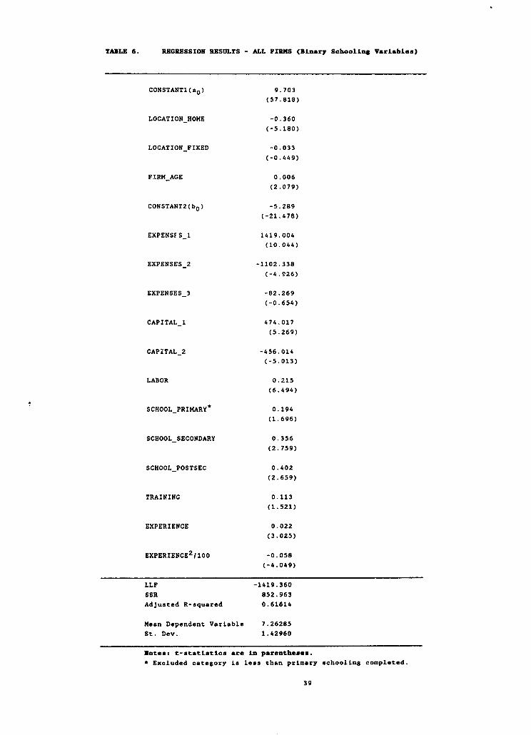
TABLE 6. REGRESSION RESULTS - ALL FIRMS (Binary SchoolLng Variables)

CONSTANT1(ao) 9.703

(57. 818)

LOCATION_HOME -0.360

(-5.180)

LOCATION_FIXED -0.033

(-0.449)

FIRM AGE 0.006

(2.079)

CONSTANT2(bo) -5.289

(-21. 478)

EXPENSES 1 1419.004

(10. 044)

EXPENSES 2 -1102. 338

(-4.926)

EXPENSES_3 -82.269

(-0.654)

CAPITAL_1 474.017

(5.269)

CAPITAL 2 -456.014

(-5.013)

LABOR 0.215

(6.494)

SCHOOL PRIMARY* 0.194

(1.696)

SCHOOL_SECONDARY 0.356

(2. 759)

SCHOOL POSTSEC 0.402

(2. 659)

TRAINING 0.113

(1.521)

EXPERIENCE 0.022

(3. 025)

EXPERIENCE21100 -0.058

(-4.049)

LLF -1419.360

SSR 852.963

Adjusted R-squared 0.61614

Mean Dependent Variable 7.26285

St. Dev. 1.42960

Notes: t-statLetics are in parenthease.

* Excluded category is less than prLmary schooling completed.

39

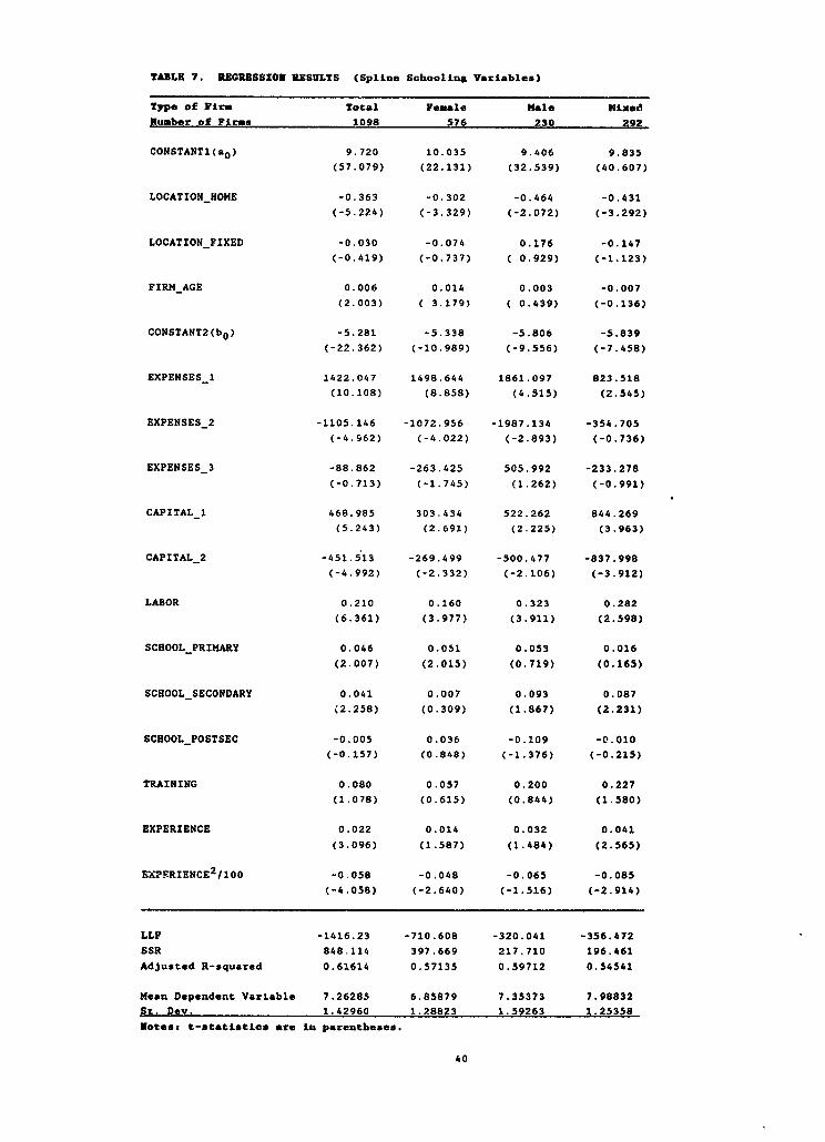
TABLE 7. REGRESSION YtESULTS (Spline Schooling Variables)

Type of Ylra Total Female Male mixed

Number of Firms 1098 576 230 292

CONSTANTl(ao) 9,720 10.035 9.406 9.835

(57.079) (22.131) (32.539) (40.607)

LOCATION HOME -0.363 -0.302 -0.464 -0.431

(-5.224) (-3.329) (-2.072) (-3.292)

LOCATION_FIXED -0.030 -0.074 0.176 -0.147

(-0.419) (-0.737) (0.929) (-1.123)

FIRM AGE 0.006 0.014 0.003 -0.007

(2.003) ( 3.179) ( 0.439) (-0.136)

CONSTANT2(bo) -5.281 -5.338 -5.806 -5.839

(-22.362) (-10.989) (-9.556) (-7.458)

EXPENSES_1 1422.047 1498.644 1861.097 823.518

(10.108) (8.858) (4.515) (2.545)

EXPENSES_2 -1105.146 -1072.956 -1987.134 -354.705

(-4.962) (-4.022) (-2.893) (-0.736)

EXPENSES 3 -88.862 -263.425 505.992 -233.278

(-0.713) (-1.745) (1.262) (-0.991)

CAPITAL_1 468.985 303.434 522.262 844.269

(5.243) (2.691) (2.225) (3.963)

CAPITAL_2 -451.513 -269.499 -500.477 -837.998

(-4.992) (-2.332) (-2.106) (-3.912)

LABOR 0.210 0.160 0.323 0.282

(6.361) (3.977) (3.911) (2.598)

SCHOOL PRIMARY 0.046 0.051 0.053 0.016

(2.007) (2.015) (0.719) (0.165)

SCHOOL-SECONDARY 0.041 0.007 0.093 0.087

;2.258) (0.309) (1.867) (2.231)

SCHOOL POSTSEC -0.005 0.036 -0.109 -0.010

(-0.157) (0.848) (-1.376) (-0.215)

TRAINING 0.080 0.057 0.200 0.227

(1.078) (0.615) (0.844) (1.580)

EXPERIENCE 0.022 0.014 0.032 0.041

(3.096) (1.587) (1.484) (2.565)

EXPFRIENCE2/100 -0.058 -0.048 -0.065 -0.085

(-4.058) (-2.640) (-1.516) (-2.914)

LLP -1416.23 -710.608 -320.041 -356.472

SSR 848.114 397.669 217.710 196.461

Adjusted R-squared 0.61614 0.57135 0.59712 0.54541

Mean Dependent Variable 7.26285 6.85879 7.35373 7.98832

St. Dev. 1.42960 1.28823 1.59263 1.25358

Notes: t-statiatics are in parentheses.

40

The pattern of signs and relative magnitudes of the estimated parameters

is quite reasonable. All levels of schooling and vocational training have

positive impacts on revenues in the binary variable model. The results suggest

there are diminishing benefits st the margin for postsecondary schooling. The

spline model tells an identical story. The fact that the third spline coefficient

is not significantly different from zero suggests that there is no important

difference (in terms of revenues) between secondary and postsecondary education.

As the sign of the linear term suggests, there are positive returns to

work experience. While these returns may initially increase, they ultimately

diminish. The fact that the quadratic term is negative implies that diminishing

returns set in more quickly. There appears to be a distinct disadvantage to

operating a business from the home as opposed to being itinerant. Finally, the

older the firm, the greater are the estimated revenues.

Labor, expenses, and capital variables continue the reasonable pattern

of results. The labor parameter has the correct sign and is highly significant.

With respect to the expenses parameters, their pattern and relative sizes are

sensible. The two spline knots for expenses were at 830 and 2,000 intis

respectively. Thus a firm with less than 830 intis in expenses will have an

expenses coefficient of 1419.004. This drops to 316.666 for a firm with between

830 and 2,000 intis of expenses, and to 234.397 for a firm with more than 2,000

intis of expenses. The fact that the coefficients decline, however, does not

guarantee that there is everywhere diminishing marginal productivity for

expenses. Eventually though, the marginal products will decline. The same is true

for capital. Here the spline knot is at 1,000 intis. Thus, a firm with less than

1,000 intis in stock and capital has a coefficient of 474.017 for aggregate

capital, and when the firm has aggregate capital in excess of 1,000 intis, the

41

coefficient is 18.003. There will eventually be diminishing returns to this

factor for all firms. Some firms in the sample, though, may be operating in a

range of increasing marginal productivity for capital.

The (ex post) tests for aggregation and pooling are identical to the ex

ante results. The hypothesis of equal structures in Lima and OUAs could not be

rejected. Similarly, the hypothesis that male, female, and mixed enterprises have

similar structures could not be rejected for all urban areas.20 An important

implication of the last test is that productivity does not differ by type of

firm. A female firm with the same factor endowments and other characteristics

as a male or mixed firm will have the same revenues, on average, as other

businesses.

6.1 Factor Productivities

The estimated revenue function provides some insights into the behavior

of factor productivity, particularly the marginal revenue products of factors.

The derivative of the revenue function with respect to a right-hand side variable

is the marginal revenue product of that variable. These derivatives will differ

from observation to observation and thus we can determine their distribution

separately for all firms, female-only firms, male-only firms, and mixed firms.

The derivatives are the product of the (unknown) price and the marginal product

of the factor. Despite the fact that the marginal products of these factors

remain unobservable, some interesting related results can be obtained for the

expected marginal revenue products.

The marginal revenue products can be thought of as shadow input prices.

A profit maximizing firm in a competitive setting would attempt to equate the

20 In all cases rural firms had significantly different structures. (See Table4).

42

marginal cost of factors (prices) with corresponding marginal revenue products.

The shadow price for a factor is deduced fr-m the marginal revenue product as

the amount the firm would be paying to the factor if the firm were being observed

at a profit-maximizing equilibrium.21

For labor, expenses, and capital we can make some conjectures about the

size of the marginal revenue products. For example, one might expect the marginal

revenue product of labor in the informal sector to be less than the wage in the

formal sector. With respect -o expenses, we might expect the shadow price to be

close to unity. Except for that part of current expenses going to purchase

stock,2 2 we would not expect any firm to spend one more inti on expenses unless

it also expected to recoup it in revenues.

For aggregate capital the case is less clear. It is difficult to deduce

dynamic effects from a static model. Nonetheless the marginal revenue product

of capital, for example, can be thought of as the rate of return to having one

more unit (inti) of, say, stock in the firm. This is over and above the price

that a firm will get when it sells the unit currently in stock. Table 8 shows

the measured marginal revenue products.

21 A further restriction for these results to hold is that the marginal revenueproduct curve is downward sloping at the profit maximizing equilibrium. If thiscondition is v4olated then the firm is not maximizing profits.

22 Unsold goods purchased with current expense money enter the inventories offirms. Our data set does not contain any information about inventory policies.

43

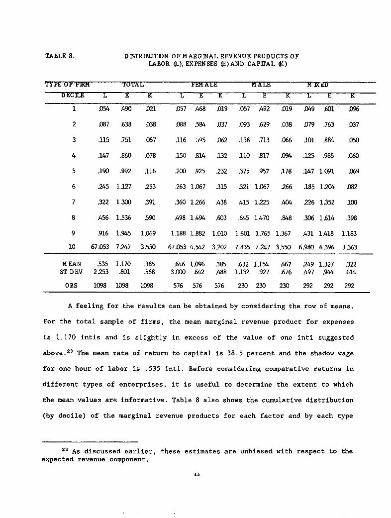
TABLE 8. D1STRIBUTDN OF MARGINAL REVENUE PRODUCTS OFLABOR (), EXPENSES E) AND CAPIrAL (C)

TYPE OF FiM TOTAL FEM ALE M ALE -- -1D

DECLE L E K L E K L E K L E K

1 .054 490 .021 .057 .468 .019 .057 .492 .019 .049 .601 .096

2 .087 .638 .038 .088 .584 .037 .093 .629 .038 .079 .763 .037

3 .115 .751 .057 .116 445 .062 .138 .713 .066 .101 .884 .050

4 .147 .860 .078 .150 .814 .132 .110 .817 .094 .125 .985 .060

5 .190 .992 .116 200 .925 .232 375 .957 .178 .147 1.091 .069

6 .245 1.127 .253 .263 1.067 .315 .321 1.067 .266 .185 1 .204 .082

7 322 1.300 .391 .360 1.266 .438 .415 1.225 .404 .226 1.352 .100

8 .456 1.536 .590 .498 1.494 .603 .645 1470 .848 .306 1.614 .398

9 .916 1.945 1.069 1.188 1.882 1.010 1.601 1.765 1.367 .431 1h418 1.183

10 67.053 7.247 3550 67.053 4.542 3202 7.835 7247 3.550 6.980 6.396 3.363

M EAN .535 1.170 .385 .646 1.096 .385 .632 1.154 .467 .249 1.327 .322ST DEV 2253 .801 568 3.000 .642 .488 1.152 .927 .676 .497 .944 .614

OBS 1098 1098 1098 576 576 576 230 230 230 292 292 292

A feeling for the results can be obtained by considering the row of means.

For the total sample of firms, the mean marginal revenue product for expenses

is 1.170 intis and is slightly in excess of the value of one inti suggested

above.23 The mean rate of return to capital is 38.5 percent and the shadow wage

for one hour of labor is .535 inti. Before considering comparative returns in

different types of enterprises, it is useful to determine the extent to which

the mean values are informative. Table 8 also shows the cumulative distribution

(by decile) of the marginal revenue products for each factor and by each type

23 As discussed earlier, these estimates are unbiased with respect to the

expected revenue component.

44

of enterprise. It is clear that all of the distributions are highly skewed and

that the mean value is typically not encountered until the seventh or eighth

decile. Thus for policy purposes the mean is not ar. informative statistic.

Moreover, before policy questions can be answered, it is necessary to determine

which firms are in the tails of the distributions (high versus low returns at

the margin), their characteristics, and the extent to which having a high (or

low) return for one variable coincides with a high (low) return for another

variable.

We analyzed the distribution of the marginal revenue products of capital,

expenses, and labor for the four sample groups: (1) all firms, (2) female-only

firms,(3) male-only firms, and (4) mixed firms. We also examined the relationship

of the marginal revenue products of factors by firm to the levels of all

productive factors. The results are presented in a set of 12 diagrams labelled

Cl, C2, C3, C4; El, E2, E3, E4; and Ll, L2, L3, L4. The letter refers the

productive factor -- capital, expenses, and labor; the number refers to the

relevant subgroup of firms above. Thus Diagram L2 shows the marginal revenue

product of labor for women-only firms.

In a representative diagram the information is: In diagram Cl, the

relevant sample is all firms, ordered from largest to smallest according to the

size of the estimated marginal revenue product of the relevant factor (in this

case, capital). Thus the firm with the largest marginal revenue product of

capital becomes the first firm and the firm with the smallest marginal revenue

product becomes the 1,098 firm. The marginal revenue product of capital is

measured on the left-hand vertical axis and, by construction, the plotted values

of the marginal revenue product of capital will decrease as higher-numbered firms

are encountered. The median firm is the $5 4 9 th and for this firm the marginal

45

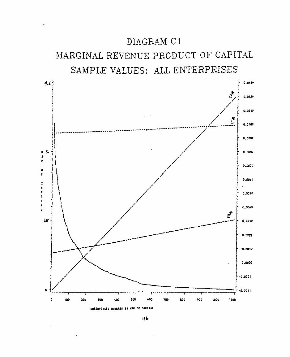
DIAGRAM C1

MARGINAL REVENUE PRODUCT OF CAPITAL

SAMPLE VALUES: ALL ENTERPRISES

!~~~~~~~~~~~~~~~~~~~~~~~~~~ Cf0.0129

1le 7X j ~~~~~~~~~~~~~~~~~~~~~~~~~~~~~~~~~~~~~~~~~~~~~~~~~~~~C.:CI 0.0099

~~~~~~~~~~~~~~~~~~~~~~~~~~~~~~~~~~~~~~ I~~~~~~~~~~~~~~~~~~~~~~~~~~~~~~~~~~~~~~~~~~~~~~~~~~~~~~~~~~~~~~~~~~~~~~~~I

A* ~~~~~~~~~~~~~~~~~~~~~~~~~~~~0.0079

4 j / f O.D069

:.rr X / _ __- "- 0.0039

_o----8zH ~ ~ ~ ~ ~ ~- - O.Ot

- - ~~~~~~~~~~~~~~~~~~~~0.0019

100 200 300 400 500 600 700 800 900 1000 1100

ENTERPRISES ORDERED SY NAP Of CAPITAL

DIAGRAM C2MARGINAL REV7ENUE PRODUCT OF CAPITAL

SAMPLE VALUES: FEMALE ENTERPRISES

o.o1o7

. 0.0097

0.J0T7

! c .

o~ i1 ./ - .:os

- j \ X t Q~~~~~~~~~~~~~~~~~~~~~~~~~~~~.0003

{.s.3 g / t ~~~~~~~~~~~~~~~~~~~~~~~~0.002t

141.~~~~~~~~~~~~~~~~~~~~~~~~~~~~~~~~~~~~~~~~~~~~~~~~~~~~~~~~~~~~~~~~~~~~~~~~~~~~~~~~~~~~~~~~~~~~~~~~~~~~~I

} / . ~~~~~~~~~~~~~~~~~~~~~~~~'-0.0003

o 4, _____ - -- - 1-- ' , ' -T-- 0 ' >0.0013

O io0 zoo 300 40 500SO

EXtERPRIME ORDERED By URP Of CAPITAL

9 I r~~

DIAGiA.iN,/ C3

-MARGINAL REVENUE PRODUCT OF CAPITAL

SA.NMIPLE VALUES: MALE ENTERPRISES

5 J ' ~~~~~~~~~~~~~~~~~~~~~~~~~~~0.0196

{ * ' ~~~~~~~~~~~~~~~~~~~~~~~~~~~~~~~~~~~0.020S_l 0.016

I F~~~~~~~~~~~~~~~~~~~~~~~~~~~~~~~~~~~~~0

0196

0.0076

r 0.0076

r 0.016

0.0106

N~~ ~ ~ .. F°0i':^

/0.0106

--. , | / L t 0.0106

P0.00 26

A 0 /t 08^6S

d \0.0076 A~~~~~~~~~~~~~~~~~~~~~ 0 .0016

/\ - ~~~~~~~~~~~~~~~~~~~~~~~~~0.0006

/ < '0~~~~~~~~~~~~~~~~~~~~~~~0.0004

/ \ '*~~~~~~~~~~~~~~~~~~~~~~~~0.0014

/ * -~~~~~~~~~~~~~~~~~~~~~~~~~0.0024/ , '-~~~~~~~~~~~~~~~~~~~~~~~~~~~~~~0. 0034

0 100 200 300

ENTERPRISES OROERED BY NRP OF CAPITAL

84

DIAGR AM C4

MARGINAL REVENUE PRODUCT OF CAPITAL

SAMPLE VALUES: MIXED ENTERPRISESf4 5

f.~~~~~~~~~~~~~~~~~~~~~~~~~~~~0.0153

1 t 0.0133

.. .. .. . .. .. .. . .. .. .. . .. .... . .. .. .. ... .. ......... ..........- -........... - L

0.0103

l 0 / k:~~~~~~~~~~~~~~~~~~~~~~~~~~.0093

A~~~~~~~~~~~~~~~~~

Pl \/ 0.0073

Iz X ,,,,-- t~~~~~~~~~~~~~~~~~~~~~~0.0063

.01~~~~~~~~~~~~~~~~~~~~~~~~~~~~~~~I

0.00.3

o A t ~~~~~~~~~~~~~~~~~~~~~0.01033

0 -, - - , - - - -, ' T - 0.0023

0 loo 200 300

ENTERPRISES OROECRED SY KRP OF CAPITAL

I~ ~~

DIAGRAAM El

MARGINAL REVENUE PRODUCT OF EXPENSE'

SAMPLE VALUES: ALL ENTERPRISES

I ~~~~~~~~~~~~~~~~~~~~~~~~~~~~0.01&7

0.0107

0.0067a r , 0.0087

0 J L0.007

-t 3. j \

,, I \ t0.0067

S [~~~~~~~~~~~~~~~~~~~~~~~~~~~~0.005?

0.0027

100 200 300 400 500 600 700 800 900 1000 1100

EUtERPRISES ORDERED BY MAP Of EXPENSES

0-

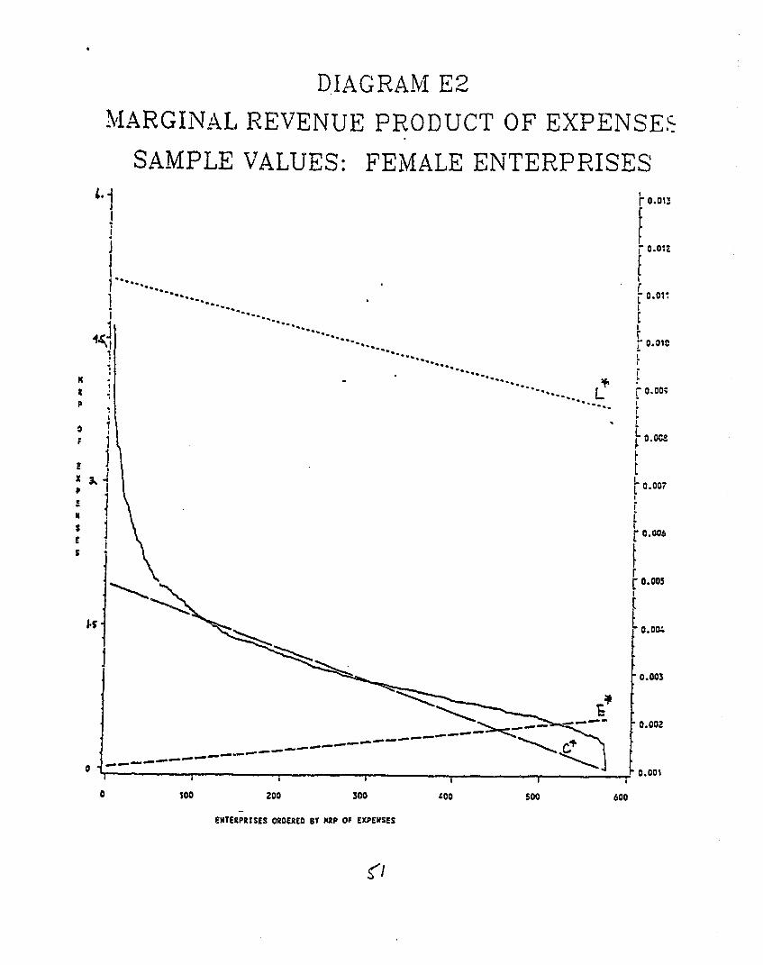
DIAGRAM E2

MARGINAL REVENUE PRODUCT OF EXPENSES

SAMPLE VALUES: FEMALE ENTERPRISES

~~~~~~~* 1 [~~~~~~~~~~~~~~~~~~~~~~~~~~'0.006

l g

.1 ~ ~ ~ ~ ~ ~ ~ ~ ~ ~ ~ ~ ~ ~ ~ ~~~~~~~~ ~~~~~0.012

*1

I.00

r 0.0102

3 ',''''"'- L ,°°°;0.002

r 1 L o.oc

IIITERPRISES ORDERED BYtXRP OF EXPENSES

.~~~~~~~~~~~~~~~~~~~~~~.0

1.5 L~~

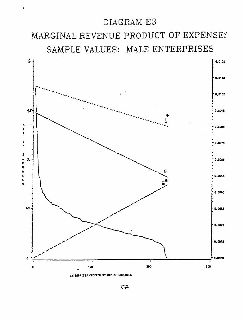
DIAGRAM E3

MARGINAL REVENUE PRODUCT OF EXPENSE.'

SAMPLE VALUES: MALE ENTERPRISES

s 0.00.9

i0 | ,,,,,, [ 0.0ca

t 11 \ .O; s. ~~~~~~~~~~~~~~~~~~~~~~~~~ ~~~0.0073

t3.n \ °°:1 0.003

O - / v ' 0.0008

s~~~~~~~~~~~~~~~~~~~~~~~~~~~~~~~~~~~~~~~~~~~~~~

0.0033

0 ~~~~~~~~~~~~ ~0,0.0008

0 100 200 300

ENTERPRISES OROERED BY NRP Of EXPENSES

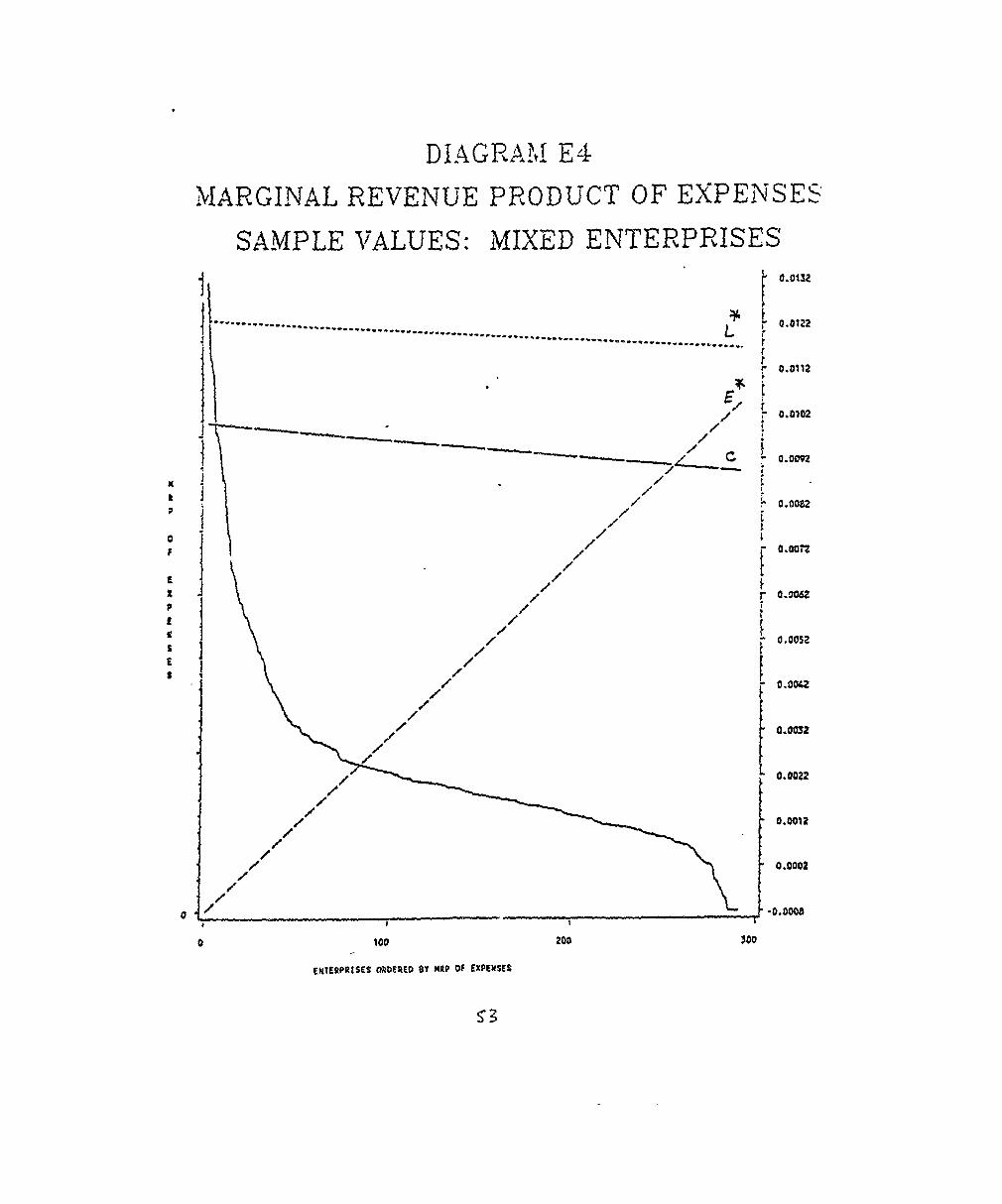
DIAGRAM E4

MARGINAL REVENUE PRODUCT OF EXPENSES

SAMPLE VALUES: MIXED ENTERPRISES

.... ~ f' ... . . . . . . . . . . . . . . . . . . . . . . . . . . . . . . . . . . . . . . . . . . .

E0 .0 1 2 2of r 0.0112

/ 0.0102

^ r c O . D~~~~~~~~~~~~~~~~~~~~~~~~~~0920.0092

w I / Oo

F

x J \

// , 0.0022

3 ,, 0.0052

/ 0.0002

30.o03z

O la0

200.00

EUIERPRISES ORDERED OY XRP Of EXPENSES

S 3

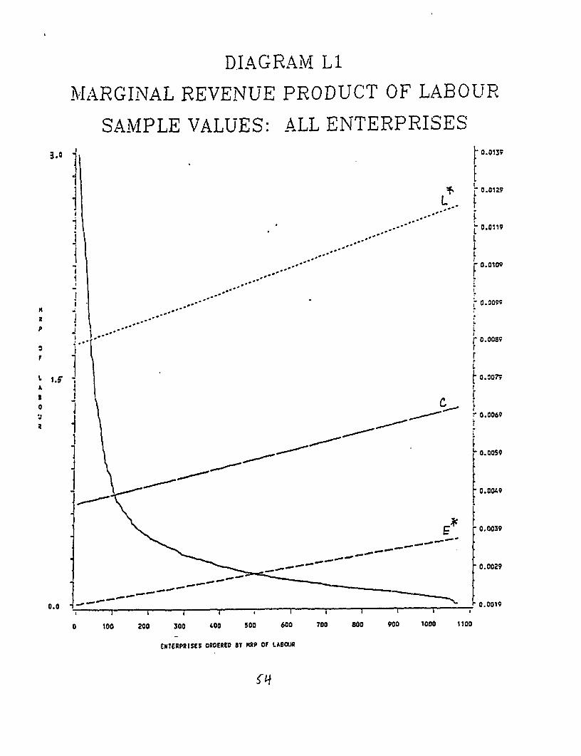
DIAGRAM Ll

MIARGINAL REVENUE PRODUCT OF LABOUR

SAMPLE VALUES: ALL ENTERPRISES3.0 i S 0.0130

al 1, 0.0129

I ~~~~~~~~~~~~~~~~~~~~~ ~~~~~~0.0109

.1 .. F°.°1°Ml - 0.00o9

1 \ ..._ < t~~~~~~~~~~~~~~~~~~~~~~~~~~ 0.00L9

0 100 200 300 400 Soo 600 700 goo 900 1000 1 t00

ENTERPRISES OROERED er PtP oF EABOUJR

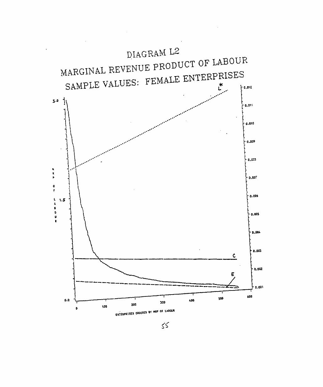
DIAGRAM L2

MARGINAL REVENUE PRODUCT OF LABOURSAIPLE VALUES: FEMALE ENTERPRISES

.0 1L V O 0

-

-Ce- -e - --------

}_0 _ wR =_ C Si ~~~~~~~~~~~~~~~~~~~O.OQ3

L ,o

aU~= ==

Ltoo

tS,R9RIStS 0OERtt as gP OF I,D6BW

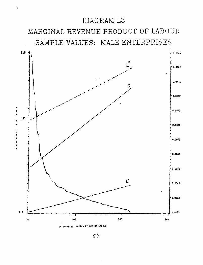
DIAGRAM L3

MARGINAL REVENUE PRODUCT OF LABOUR

SAMPLE VALUES: MALE ENTERPRISESO .013Z

F-~~~~~~~~~~~~~~~~~~~~~~~~~~~~~~~~~~~~~~~~~~~~~0.0102J~~~~~~~~~~~~~~~~~~~~~~~~~~~~~~~~~~~~~~~~~

J~~~~~~~~~~~~~~~~~~~~~~~~~~~~~~~~~~~~~~~~~

N I / i.07

* ' 0.00S

p

I 0

a K

0.0 _- 0

EE

0.0032

0 100 200 300

ENTERPRISES ORDERED BY KRP Of LABOWR

('(9

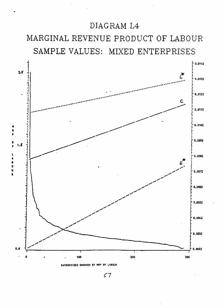
DIAGRAM L4

MARGINAL REVENUE PRODUCT OF LABOUR

SAMPLE VALUES: MIXED ENTERPRISES

' ,,,,,,_,,,.-J-"''''"''''''''" ~~~~~~~~~~~~~00122I~~~~~~~~~~~~~~~~~~~~~~~~~~~~~~~~~~~~~~~~~~~~~~~~~~~~~~~~~~~~~~~~~~~~~~~~~~~~~~~~~~~~~~~~I

0.0t22

0 1.5 . , 0112

.L o 0.0052

A~~~~~~~~

N '-/ 0.002

p.~~~~~~~~~~~~~~~~~~~~~~~~~0

/// ~~~~~~~~~~~~~~~~~~~~~~~0.0032

0 1~~~~~~~~.0

.00,~~~~~~~~~~~~~~~~~~~~~~~~~~008

0.0022

0 . _ 100 200 300

ENTERPRISES ORDERED BY HRP OF LA8LUR

'7

revenue product is about .15 inti. Notice how quickly the marginal revenue

product of capital by firm declines as we consider the first 200 firms.

Next consider the relationship of the marginal revenue products to the

levels of the productive factors. Capital, expenses, and labor variables are

all measured on the right-hand vertical axis. The variables were scaled to all

fit on these axes. The lines C, E and L represent the least squares regression

lines of the capital, expenses, and labor variables (respectively) of firm i on

the rank (1 to 1,098) of firm i. The rank of a firm continues to be determined

by the size of its marginal revenue product. An asterisk in the label of a

regression line indicates that the slope of the regression line is significantly

different from zero.

These regression lines provide a considerable amount of additional

information that explains the distributions of the marginal revenue products.

In diagram Cl we see that firms with high marginal revenue products of capital

also had significantly lower endowments of capital. They also tended to have

significantly lower quantities of expenses and labor. Extending the analysis to

capital input for female enterprises (diagram C2), we see that firms with high

marginal revenue products of capital had significantly lower endowments of

capital. There is, however, no significant relationship between the distribution

of the marginal revenue products and either expenses or labor.

Two patterns can be isolated in the marginal revenue product diagrams.

First, for all groups of firms and for all productive factors there is a

significant relationship between the marginal revenue product of a factor and

the amount of the factor. Firms with smaller amounts of a given factor tend to

have higher marginal revenue products for the factor. Second, in about 75 percent

of the cases where a significant relationship exists, there is an inverse

58

relationship between the marginal revenue product of one factor and the

quantities of the other factors. This suggests that small firms are the most

productive in terms of measured marginal revenue products.

These results have important implications for the competitive structure

of the informal urban retail sector. The sector's rapid growth may well signal

a greater degree of competitiveness in retail trade, and large incumbent firms

may be feeling the pressure of both inefficient size and falling (real) prices.

Leaner and more aggressive small firms appear to be making significant inroads.

Some supporting evidence for this view comes from examining the location

structure of firms in the upper and lower 20 percent tails. Firms with low

returns to labor and capital are much more likely to operate out of homes and

fixed locations while those with high returns are mobile. For the capital

variable, firms in the upper tail are twice as likely to be mobile as firms in

the lower tail. And female-only firms tend to have lower capital, labor, and

expenses than male-only and mixed firms. It appears that women are good

candidates for the high rates of return obtained by smaller firms. It may be,

however, that these returns at the margin can be further increased. Female firms

may be operating where marginal revenue product curves have a positive slope.

In this case growth would tend to make these firms even more productive.

6.2 Nonparametric Evidence

These estimates are based on parametric methods. The results below are

based on a nonparametric approach (described in appendix B). That estimates

marginal revenue products and revenue without having to specify (parametric)

model. In the nonparametric analysis all the variables appearing in the

parametric model were included except dummy variables. Since the nonparametric

59

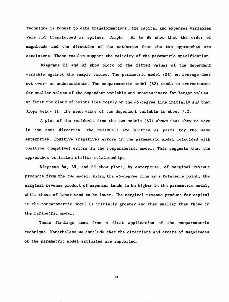
technique is robust to data transformations, the capital and expenses variables

were not transformed as splines. Graphs Bi to B6 show that the order of

magnitude and the direction of the estimates from the two approaches are

consistent. These results support the validity of the parametric specification.

Diagrams B1 and B2 show plots of the fitted values of the dependent

variable against the sample values. The parametric model (Bi) on average does

not over- or underestimate. The nonparametric model (B2) tends to overestimate

for smaller values of the dependent variable and underestimate for larger values.

At first the cloud of points lies mostly on the 45-degree line initially and then

drops below it. The mean value of the dependent variable is about 7.2.

A plot of the residuals front the two models (B3) shows that they to move

in the same direction. The residuals are plotted as pairs for the same

enterprise. Positive (negative) errors in the parametric model coincided with

positive (negative) errors in the nonparametric model. This suggests that the

approaches estimated similar relationships.

Diagrams B4, B5, and B6 show plots, by enterprise, of marginal revenue

products from the two model. Using the 45-degree line as a reference point, the

marginal revenue product of expenses tends to be higher in the parametric model,

while those of labor tend to be lower. The marginal revenue product for capital

in the nonparametric model is initially greater and then smaller than those in

the parametric model.

These findings come from a first application of the nonparametric

technique. Nonetheless we conclude that the directions and orders of magnitudes

of the parametric model estimates are supported.

60

DIAGRAM Bi

PARAMETRIC FIT

10 ++ +

E9'] + +++

. +F ~ ~++4

T 44 5 6 9 1

1 8~ ~ ~~~6

T

ET *+ + ++

D 7

+ *+~~~~~~~V + ++: :~+ A

L 6 ++ + 4t 4 +** ~

s + 4++p ~+~ F+

3

3 4 5 6 7 8 10

ACTUAL VALUES

DIAGRAM B2

NONPARAMETRIC FIT

' 8F + +t

T + ++T +

D 7 *

6 + + ? 8 9 10

4

3

3 a 9 10

ACTUAL VALUES

DIAGRAM B3

COMPARISON OF MODELSRESIDUALS

3

N +

r:1 + + +

A , + + ++

N +' + se + +A +

E + + +T +

L + +

c + a+$ + 4.

R

C +IA

D 6

A

-2 ~ ~1 0 1 23

PARAMETRIC RESIDUALS

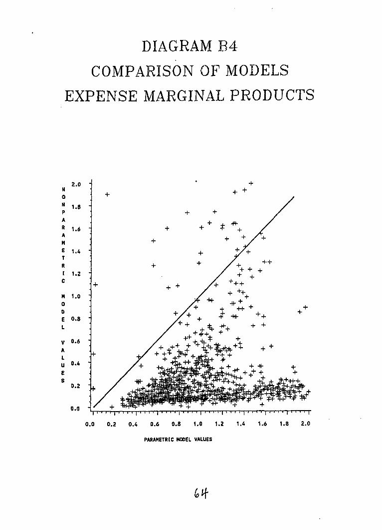
DIAGRAM B4

COMPARISON OF MODELS

EXPENSE MARGINAL PRODUCTS

2.0 ' +N ~~~~~~~~~++

m + +0 +N 1.8-+ +/p + +A +R + + +*4

A + + + .+E 1.4 + + +T ++R + + ++1 1.2 + + +C + +

M1.0 + +0 .+ +0 + + +E 0.8 ++++

L *~~~~~+ +* + +

V 0.6 ++ ++

U 0.4

+

0.2 +

0.0 0.2 0.4 0.6 0.8 1.0 1.2 1.4 1.6 1.8 2.0

PARAM4ETRIC MOOEL VALUES

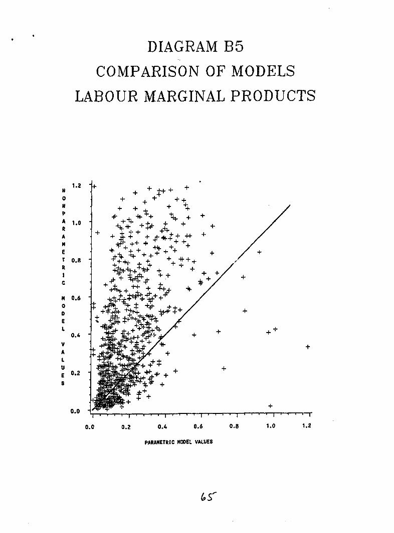
DIAGRAM B5

COMPARISON OF MODELS

LABOUR MARGINAL PRODUCTS

N 1.2 + + +

0 + ++

N + + + ++p ++A 1.0 +T +

00 +F . + +A 4-;+ + 4+ + + +N +~~~++ + +~-1++ ++

0.0 0 . + + 0 R +~~-* ,4 + + *++fI 4 ~1 ~4+ yi- +* + +

C ++R + Y

0.6600 +

0. + + ++0V +

A L

U +

+~~~~~~~

0.0

0.0 0.2 0.4 0.6 0.8 1.0 1.2

PARAMETRIC MODEL VALUES

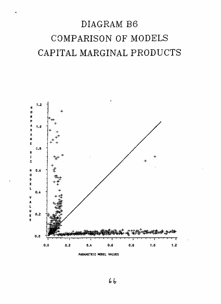
DIAGRAM B6

COMPARISON OF MODELS

CAPITAL MARGINAL PRODUCTS

1.2Na +N. p

A 1.0

A +/A .N ~+

E + +

+ ~~~~~~~~+C + / +

+E ~+

N 0.6

D /

0.4V +X

UD /

SE0.2

0.0 0.2 0.4 0.6 0.8 1.0 1.2

PARAMETRIC MWEL VALUES

b

6.3 Simulation Experiments

The estimated revenue model can address a variety of other questions. For

example, it can assess the impact of policies that affect Lhe amount, quality,

and distribution of productive factors such as loans (either unrestricted or

factor-specific) to a given subgroup. Evaluating such a credit policy would

invclve estimating the effects on expected revenues and determining the payback

period for the loan. Policymakers can also assess the revenue impact of social

policies that raise education levels or allow family members to substitute work

in the family business for housework (perhaps through child care programs).

Table 9 shows the effects on expected revenues, averaged over firms, of

seven different policy experiments. The first four experiments are 'simple' in

that only one underlying variable is changed. The other four experiments are

'compound' in that more than one variable changes. For example, in the first

experiment, the most educat-d individual in the firm is given two more years of

schooling if the number of years of schooling is less than nine. The group of

firms receiving this education changes from all firms, to the bottom 50 percent

(in terms of education), and then to the bot om 25 percent (in terms of

education) and finally, for comparison purposes, to the top 25 percent. Within

each group, the effects on all, female firms, male firms, and mixed firms are

calculated separately. The effect of formal schooling on revenues is 100 to 200

intis a month.

The second simulation increases the amount of labor by 100 hours a month.

This could be accomplished by policies that reduce the costs of noncompliance,

encourage bulk purchasing by cooperatives, and offer training in management.

The time devoted to business activities by women could be increased by providing

67

Table 9. SIMULATION RESULTS - EFFECTS ON REVENUES

INCREASE IN BY I (1) 1 (2) 1 (3) 1 (4) 1 (5) 1 (6 1 17 l

Years of Schooling 2 2

Monthly Hours 100 100 100

Expenses S 1000 500 500 500

Total Capital $ .I 1000 500 500 500

_ I -I .INobs S Nobs S Nobs S Nobs S Nobs S Nobs S Nobs S

Glven to AllFLrmsb Y

All Enterprises 11098 103 1098 187 1098 1079 1098 31411098 843 1098 1100 1098 1245

Female Enterprises 576 97 576 182 576 988 576 323 576 828 576 1101 576 1250

Male Enterprises 230 112 230 237 230 1136 230 399 230 907 230 1255 230 1377

Mixed Enterprises 292 109 292 157 292 1213 292 231 292 820 292 1001 292 1130

GLven to Bottom 50 Z of Firms

All Enterprises 528 157 546 239 549 1279 549 578 755 872 845 1001 926 1039

Female Enterprises 343 126 366 218 361 1102 358 495 471 810 514 977 538 1057

Male Enterprises 100 175 127 299 111 1394 125 690 165 908 195 1030 209 1074

Mixed Enterprises 85 2601 53 243 77 1944 66 816 119 10701 136 1052 179 943

Given to Bottom 25 1 of Flrms I lAll Enterprises 242 1441 274 284 274 1409 274 641 446 6691 541 737 637 695

Female Enterprises 180 119| 197 257 163 1176 182 588 281 5671 347 650 411 6151

Male Enterprises 40 199 67 363 71 1449 72 671 109 7291 131 843 145 8321

Mixed Enterprises 22 248 10 267 40 2285 20 1011 56 1068 63 998 81 853

Given to Top 25 2 of Firms I IAll Enterprises 146 42 274 115 274 978 274 58 421 3341 522 330 577 309|

Female Enterprises 47 32 75 104 81 973 82 49 138 296 181 270 210 239

Male Enterprises 36 40 27 114 61 988 59 58 96 328 108 321 121 2991

Mixed Enterprises 63 50 172 120 132 975[ 133 641 187 3641 233 3821 246 3741

Notes: The bottom 50X refers to those firms that have less than the median value of the variables)

of interest for all firms. For example, if $1000 of expenses is provided, then only those firms with

less than the median value of expenses ($806) receive the $1000. The same applies to the bottom 25X

and the top 252. The median and quartile values are:

Median Bnttom 25X Top 252

Years of Schooling 7.0 4.0 10.0Monthly Hours 234.0 113.6 386.3

Expenses $ 805.6 247.2 2478.3

Total Capital $ 967.7 170.5 4337.8

cooperative child care and facilities for meals. This experiment suggests that

revenues will increase by a respectable 200 to 300 intis a month, especially

among firms in the bottom 50 and 25 percent (in terms of labor).

The third simulation lends 1,000 intis to selected firms for operating

expenses. The results are impressive. If all firms receive the loan, on average

68

they will be able to repay the loan, retaining 79 intis as net profit for the

month. Alternatively, because they are more productive, when only the lowest

quartile (in terms of expenses) receive the loans, the average net profit is 409

intis. The small number (40 firms) of mixed enterprises in this quartile would

be the most successful, with an average net profit of 1,285 intis for the month,

compared to 176 intis for the 163 female businesses, and 449 intis for the 71

male firms.

When interpreting the fourth experiment, (each firm receives 1,000 intis

for capital expansion), the fact that the average return is less than 1,000 intis

does not mean the policies are not successful. The funds would be used to acquire

capital that would not completely depreciate in a month. In fact, the ratio of

1,000 intis to the average monthly increase in revenues is the average payback

period for the loan in months assuming zero economic depreciation. For example,

all enterprises would take just over three months (1,000/314) on average to repay

the loan. It should be noted, however, that firms with low capital endowments,

mostly female firms, tend to perform better than those with high endowments. Two-

thirds of the firms in the lowest quartile are female businesses, with an

estimated payback period of less than two months (1,000/588). The payback period

for firms in the top quartile is about 18 months (1,000/58).

The remaining 'compound' experiments (five, six, and seven ) largely

conifirm the 'simple' ones. The effects on predicted revenues of firms with lower

endowments of expenses, capital, and labor are generally higher than three of

better-endowed firms.

Finally, in comparing the simulated increases in revenues it is important

to examine more than just the average increases. There are disttibutions

associated with these point estimates. Standard statistical testing shows few

69

significant differences among the three types of firms, but this was not the

case among firms in different quartiles.

The simulation results in Table 9 are quite similar to those obtained in

the analysis of factor productivity discussed earlier. These results are very

helpful in terms of quantifying the effects of policies for the informal sector.

It appears a policy of loans to poorly endowed firms, most of which are female

businesses, could offer significant social gains.

7. Policy Implications

The extent to which estimated productivity differs among male, female,

and mixed firms appears to be due more to the distribution of factors across

enterprises than to any inherent advantage or disadvantage in the type of firm.

On average, the productivity of female firms is neither better nor worse than

that of male or mixed firms with the same factor endowments (capital, expenses,

and labor). The influence of these endowments, however, affects productivity more

than the gender or education of the entrepreneurs. Firms with smaller endowments

tended to have higher factor productivity. Thus the process of retailing is the

same among firms, but the endowment effect makes them different. Put another way,

firms with less capital, expenses, or labor usually have higher returns at the

margin but typically lower revenues. As seen in Table 3 or Table 9, a high

proportion of female firms, but a much smaller proportion of male and mixed

firms, have low amounts of capital, expenses, and labor. In our sample about a

fourth of the businesses had little or no capital and a third carried no

inventories -- most of these were female firms. The empirical analysis suggests

that proactive policies would increase substantially the productivity of small

70

businesses. Providing assistance to small businesses makes good economic sense -

- particularly if directed to those with low factor endowments.

The ultimate objective of policy measures is to alleviate poverty and

improve household welfare. Improving productivity in the informal sector helps

to achieve this goal. While we do not elaborate on implementation, two directions

will be effective. First enterprise-specific policies that directly affect

productivity, and second, set of policies aimed at women that address the

competing demands on their time.

7.1 Enterprise-Specific Policies

Governments and international donors have primarily assisted small

businesses by providing low-cost credit to firms that do not have access to

formal financial markets. Loans are small -- usually less than $500 -- but there

are many beneficiaries. Results are good and the repayment rate is often more

than 90 percent. Our estimates of productivity confirm that channeling credit

to small businesses is effective in raising productivity. Examples of different

credit programs include the Grameen Bank in Bangladesh, the Self-Employed Women's

Association in India, the Banco Popular in Costa Rica, the Badan Kredit Kecamatan

in Indonesia, the Northeast Union of Assistance to Small Businesses in Brazil,

the Institute for the Development of the Informal Sector in Peru, Fondo de

Fomento para la Pequena Industria y la Artesania in Ecuador, and the Small

Projects Program of the Inter-American Development Bank.24

Another way to help small businesses is by promoting cooperatives and

self-help associations. In addition to providing credit these organizations can

24 See Cornia (1987), Everett and Savara (1986), Herz (1989), Hossain (1987),IDB (1988), Tendler (1983), United Nations (1985), and World Bank (1989).

71

make bulk purchases from wholesalers, provide storage facilities for perishable

or nonperishable commodities, and establish markets for entrepreneurs (see

Bunster and Chaney 1985, de Soto 1989).

Technical assistance programs are a third option, offering short-term

instruction in basic management, including keeping records, marketing,

purchasing, and dealing with municipal authorities and other formal sector

institutions. Inter-American Development Bank (1988) notes that instruction can

be provided informally at neighborhood markets or at the business site,

Most family businesses in Peru are clandestine operations that generally

avoid complying with regulations. The performance o2 these businesses could be

-mproved by reducing the costs of non compliance. This would mean eliminating

various forms of harassment by local authorities, and simplifying the process

of conforming to the laws (for example, by making it easier and less costly to

obtain a business license).2 5

7.2 Women-Specific Policies

Although enterprise-specific policies can improve the productivity, they

may have undesirable side-effects in those instances where women operate or work

in the business. Most of these women also have household responsibilities and

children, end inevitably these obligations entail conflicting demands.

Enterprise-specific policies may inadvertently encourage women to devote

more time to the firm, leaving them with less time for activities related to

health, nutrition, education, and child care. Hence these policies may have

negative effects on household welfare in general and child welfare in particular

(Cornia 1987, Jolly and Cornia 1984).

25 For discussions see Bunster and Chaney (1985), de Soto (1989), Mescher(1985), Tinker (1987), and World Bank (1987).

72

These negative effects can be mitigated by a complementary set of women-

specific policies directed toward reducing the workload associated with home

activities. These may enhance the firm's productivity by allowing women to devote

more time to the business. Cornia (1987) discusses such programs in Latin

America. Coopetative child care centers ("clubes de madres"), facilities for the

preparation of food ("comodores populares"), and neighborhood facilities for

basic health care will improve the firm's productivity.

This study suggests that proactive policies and projects to help small

firms will result in social gains, contribute to the alleviation of economic

hardship, and enable disadvantaged -- especially women -- to become effective

agents in the development process.

73

Appendix A: Nonparametric Analysis

A nonparametric approach provides an alternative to the parametric model

presented in the paper. The specification of functional forms is not required

in nonparametric modeling, while in parametric modeling a functional form is

explicitly defined. Also, under certain regularity conditions, the nonparametric

estimates are consistent. This contrasts with the least squares approach where

any misspecification of the functional form, however minor, will lead to

inconsistent parameter estimates. It is not possible to say that nonparametric

methods are more or less powerful than parametric methods -- the technique may

provide a different explanation of the data. When parametric and nonparametric

models provide similar results, it is reasonable to hold a stronger belief in

the validity of the parametric specification.

Nonparametric Modeling

Consider the model:

Yi -g(X) + ui i = l. ,n (17)

where YL is the ith observation of the dependent variable Y and X. is the ith row

of the matrix of explanatory variables, X. There are k explanatory variables

and n observations on each dependent and independent variable. The unobserved

error term for the ith observation is u.

The parametric approach to estimating this model involves specifying a

functional form for go and then applying a least squares or maximum likelihood

algorithm to obtain point estimates of the parameters. The results of such an

approach were presented in the paper.

74

The nonparametric approach to estimat..ng (17) starts with the observation

that the model could be written equivalently as:

Y- g(XL) + U-

- E(YJIXd) + UL (18)

where g(X) - E(Yi1Xi) is the expectation of Y1 conditional upon X.. This is

also called the conditional mean of Y. The researcher estimates the model in

(17) or (18) and its properties by estimating the conditional mean and how the

conditional mean depends upon the conditioning varirbles. Technioues exist for

estimating the conditional mean without specifying a particular functional form

for go. Of course, different distribution and regularity assumptions are

introduced. In particular, the independent variables (drawings from which form

the conditioning matrix X) are typically assumed, but not required, to be Jointly

distributed random variables. As well, continuity and differentiability

assumptions are often implicit in the estimation of the conditional mean

function.

The following is a brief description of the nonparametric approach. The

reader is referred to Ullah (1988) for a more complete -discussion of the

development and use of nonparametric techniques in economics.

Defining Conditional Means and Their Properties

Suppose that the vector of random variables (Y, X) has a joint density

function given formally by:

dProbl(Y,X) < (y,x)]f(y,x) - (19)

d(y,x)

The marginal density function for X is defined by:

fl(x) .ff(y,x)dy (20)

75

Finally, the conditional density function of Y given X is defined by:

f(ylx) - V.x) (21)fl(Z')

Using these definitions, the conditional mean introduced in (18) is givenby :

E(ylx) - fyf(ylx)dy

r f(y ,x)- IY__dyJ fl(x) (22)

In a similar fashion, the vector of changes or responses of the

conditional mean to a change in the vector of realizations of X. is given by:

dE(YIX) d [f(y,x,)== - - ![Y dy

dxL dox J f 1 (XL) (23)

The parametric analogue of the vector of derivatives of the conditional

mean with respect to the realizations of the explanatory variables is the vector

of derivatives of the dependent variable with respect to the independent

variables. In terms of our revenue model, they are the marginal revenue products

of the factors.

Estimating Conditional Means and Derivatives

Equations (22) and (23) show that the only information required to

estimate the conditional means and the derivatives is the joint density function

f(y,x). Once this is available, the marginal density can be computed (as in (20))

and all the right hand side of (22) is known. As (21) shows, the derivative on

the right hand side of (23) can be computed and the integral can then be

evaluated.

76

There are many ways to estimate a multivariate density function. For

example it is possible to generalize the one-dimensional technique for obtaining

histograms. However, the resulting density estimate will not be differentiable.

More popular techniques involve kernel estimators. Formally, the estimate of the

multivariate density f(w) = f(y,x), where W. = (Yt,X 1 ) is given by:

A nf(w) - (1/nhq)E K((W1 - w)/h) (24)

i-1

where: h is the window width, n is the number of observations, q is the number

of elements in any W. (equal to the number of explanatory variables, k, plus

one for the dependent variable) and K() is the kernel function. The kernel

function is typically taken from the set of many times differentiable

multivariate density'functions. One popular kernel function is the multivariate

normal or Gaussian density. Note, however, that the choice of a Gaussian kernel

in no way restricts the estimated density. Indeed, it would appear that density

estimates are much less sensitive to the kernel function than they are to the

window width, h. The choice of the window width determines, in part, the degree

of smoothing of the densicy estimate. Recent work by Racine (1989) has examined

the optimal window width, h, in the sense of integrated mean square error. The

results for the Peru Living Standards Survey data make use of this optimal window

width and a Gaussian kernel.

77

Appendix B: The Rural Model

We have attempted to fit the revenue model to the rural data.26 The results

show definite similarities to the results arising in the urban data, but we are

somewhat less confident that the rural results are robust.

Table B2 shows the parameter estimates for the model.27 It is apparent

that the pattern of signs for those parameters estimated with some precision

(that is, those with t-statistics more than 2) is similar to that in the urban

data. For example, labor, capital and expenses (materials) have positive marginal

products everywhere. But only 7 of 17 parameters are estimated with precision

as opposed to 13 of 17 in the urban data. The model explains 59 percent of the

variation in the dependent variable. This compares well with the corresponding

61 percent for the urban model.

We computed values for the marginal revenue products of labor, capital,

and expenses for every observation in the sample of 288 rural businesses. Table

B3 gives the means, standard deviations, and decile values for the distributions

of these derivatives in the sample. These values can be compared with

corresponding results for the urban model presented in Table 4. In general, the

marginal revenue products for rural firms are lower than those for urban firms;

the rural values for labor and expenses are about 80 percent of the urban levels,

and the rural values for capital are almost the same as the urban levels. Tne

troubling statistical feature of the rural model is that many of the data points

may be highly influential. Of the 288 observations, 56 data points (20 percent

26 Table Bl contains information on the variables entering the rural model; theformat of is identical to that of urban areas.

27 We present results for the case where dummy variables are used to distinguishschooling levels.

78

of the sample) need detailed examination. Our concern arises from two sources:

the data have high measured leverage, and the regression residuals are large in

absolute value. The sheer number of these points combined with the costs of

reestimating the nonlinear model to examine the importance of these points

individually and in groups led us to concentrate our efforts instead on the urban

model.

We do not argue that the estimates of the rural model are wrong. Indeed,

as noted above, the pattern of results and other similarities with the urban

results provide strong indirect evidence of their qua.ity. We note, h,wever, that

the diagnostic evidence in support of the rural model is not as strong as that

for the urban model.

79

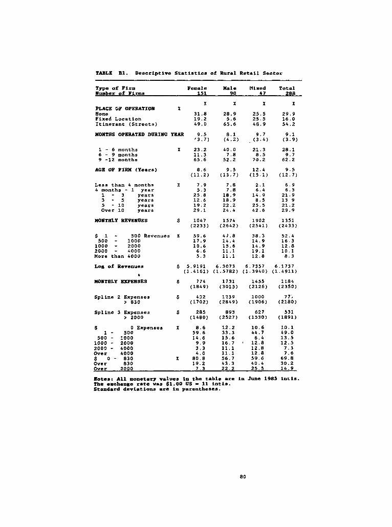
TABLE BI. DescriptLve Statistics of Rural Retail Sector

Type of FLrm Female male kixed TotalNumber of Flrms 151 90 47 288

x X X XPLACE C5F OPERATION XHome 31.8 28.9 25.5 29.9Fixed LocatLon 19.2 5.6 25.5 16.0Itlnerant (Streets) 49.0 65.6 48.9 54.2

MONTHS OPERATED DURING YEAR 9.5 8.1 9.7 9.1'3.7) (4.2) (3.4) (3.9)

1 - 6 months X 23.2 40.0 21.3 28.16 - 9 months 11.3 7.8 8.5 9.79 -12 months 65.6 52.2 70.2 62.2

AGE OF FIRM (Years) 8.6 9.5 12.4 9.5(11.2) (13.7) (15.1) (12.7)

Less than 4 months X 7.9 7.8 2.1 6.94 months - 1 year 5.3 7.8 6.4 6.3

1 - 3 years 25.8 18.9 14.9 21.93 - 5 years 12.6 18.9 8.5 13 95 - 10 years 19.2 22.2 25.5 21.2Over 10 years 29.1 24.4 42.6 29.9

MONTHLY REVENUES 5 1047 1574 1902 1351(2233) (2642) (2541) (2433)

$ 1 - 500 Revenues X 59.6 41.8 38.3 52.4500 - 1000 17.9 14.4 14.9 16.31000 - 2000 10.6 15.6 14.9 12.82000 - 4000 6.6 11.1 19.1 10.1More than 4000 5.3 11.1 12.8 8.3

Log of Revenues $ 5.9191 6.3073 6.7357 6.1737(1.4161) (1.5782) (1.3940) (1.4911)

MONTHLY EXPENSES $ 774 1731 1455 1184(1849) (3015) (2126) (2350)

Spline 2 Expenses $ 432 1739 1000 77;> 830 (1702) (2849) (1906) (2180)

Spline 3 Expenses $ 285 893 627 531> 2000 (1480) (2527) (1530) (1891)

$ 0 Expenses X 8.6 12.2 10.6 10.11 - 500 59.6 33.3 44.7 49.0

500 - '000 14.6 15.6 6.4 13.51000 - 2000 9.9 16.7 12.8 12.52000 - 4000 3.3 11.1 12.8 7.3Over 4000 4.0 11.1 12.8 7.6$ 0 - 830 2 80.8 56.7 59.6 69.8Over 830 19.2 43.3 40.4 30.2Over 2000 7.3 22.2 25.5 14.9

Notest All monetary values in the table are in June 1985 lntis.The exchange rate was $1.00 US - 11 intis.Standard devlations are in parentheses.

80

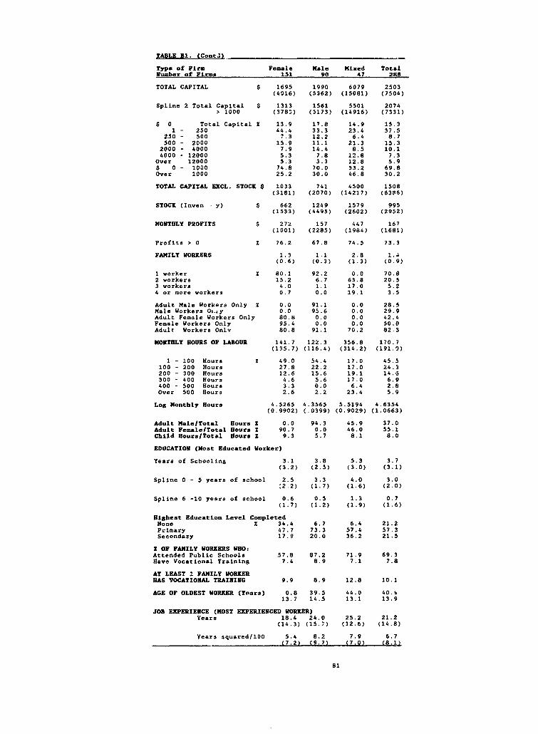
TABLE B1. (Conti)_

Type of Plrs Female male Mixed TotalNumber of Firms 151 90 47 288

TOTAL CAPITAL $ 1695 1990 6079 2503(4016) (5362) (15081) (7504)

Spline 2 Total Capital $ 1313 1561 5501 2074> 1000 (3783) (5173) (14916) (7331)

5 0 Total Capital X 13.9 17.8 14.9 15.31 - 250 44.4 33.3 23.4 37.5

250 - 500 7.3 12.2 6.4 8.7500 - 2000 15.9 11.1 21.3 15.3

2000 - 4000 7.9 14.4 8.5 10.14000 - 12000 5.3 7.8 12.8 7.3

Over 12000 5.3 3.3 12.8 5.9$ 0 - 1000 74.8 70.0 53.2 69.8Over 1000 25.2 30.0 46.8 30.2

TOTAL CAPITAL EXCL. STOCK 1033 741 4500 1508(3181) (2070) (14217) (63ft6)

STOCK (Inven y) $ 662 1249 1579 995(1533) (4495) (2602) (2952)

MONTHLY PROFITS $ 272 157 447 167(1001) (2285) (1984) (1681)

Proflts > 0 t 76.2 67.8 74.5 73.3

FAMILY WORKERS 1.3 1.1 2.8 1.4(0.6) (0.3) (1.3) (0.9)

1 worker I 80.1 92.2 0.0 70.82 workers 15.2 6.7 63.8 20.53 workers 4.0 1.1 17.0 5.24 or more workers 0.7 0.0 19.1 3.5

Adult Male Workers Only X 0.0 91.1 0.0 28.5Male Workers Ot.sy 0.0 95.6 0.0 29.9Adult Female Workers Only 80.8 0.0 0.0 42.4Female Workers Only 95.4 0.0 0.0 50.0Adult Workers Onlv 80.8 91.1 70.2 82.3

MONTHLY HOURS OF LABOUR 141.7 122.3 356.8 170.7(135.7) (116.4) (314.2) (191.0)

1 - 100 Hours X 49.0 54.4 17.0 45.5100 - 200 Hours 27.8 22.2 17.0 24.3200 - 300 Hours 12.6 15.6 19.1 14.6300 - 400 Hours 4.6 5.6 17.0 6.9400 - 500 Hours 3.3 0.0 6.4 2.8Over 500 Hours 2.6 2.2 23.4 5.9

Log Monthly Hours 4.5265 4.3565 5.5194 4.6354(0.9902) (.0399) (0.9029) (1.0663)

Adult MalelTotal Hours X 0.0 94.3 45.9 37.0Adult Female/Total sours Z 90.7 0.0 46.0 55.1Child Hours/Total Bours Z 9.3 5.7 8.1 8.0

EDUCATION (Most Educated Worker)

Years of Schooling 3.1 3.8 5.3 3.7(3.2) (2.5) (3.0) (3.1)

Spline 0 - 5 years of school 2.5 3.3 4.0 3.0:2.2) (1.7) (1.6) (2.0)

Spline 6 -10 years of school 0.6 0.5 1.3 0.7(1.7) (1.2) (1.9) (1.6)

Bighest Education Level CompletedNone X 34.4 6.7 6.4 21.2Primary 47.7 73.3 57.4 57.3Secondary 17.9 20.0 36.2 21.5

Z OF PAMILY WORKERS WHO:Attended Public Schools 57.8 87.2 71.9 69.3Have Vocational Training 7.4 8.9 7.1 7.8

AT LEAST : FAMILY WORKERHAS VOCATIONAL TRAINING 9.9 8.9 12.8 10.1

AGE OF OLDEST WORKER (Years) 0.8 39.5 44.0 40.%13.7 14.5 13.1 13.9

JOB EXPERIEBNCE (MOST EXPERIENCED WORKER)Years 18.4 24.0 25.2 21.2

(14.3) (15.7) (12.6) (14.8)

Years squaredl100 5.4 8.2 7.9 6.7(7.2) (9.7) (7.0) (8.1)

81

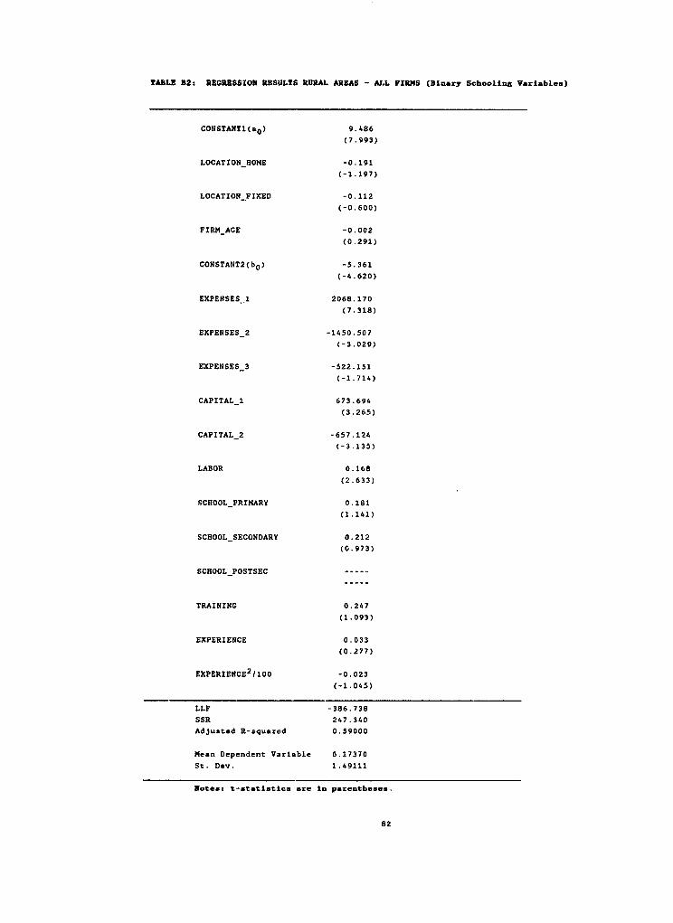
TABLE 32: REGRESSION RESULTS RURAL AREAS - ALL FIRMS (Binary Schooling Variables)

CONSTANTl(ao) 9.486

(7.993)

LOCATION_HOME -0.191

(-1. 197)

LOCATION-FIXED -0.112

(-0.600)

FIRM AGE -0.002

(0 291)

CONSTANT2(bo) -5.361

(-4.620)

EXPENSES 1 2068.170

(7.318)

EXPENSES_2 -1450.507

(-3.029)

EXPENSES 3 -522.151

(-1.714)

CAPITAL 1 673.694

(3.265)

CAPITAL 2 -657.124

(-3.135)

LABOR 0.168

(2.633)

SCHOOL PRIMARY 0 .181

(1.141)

SCHOOL-SECONDARY 0.212

(0.973)

SCHOOL_POSTSEC

TRAINING 0.247

(1.093)

EXPERIENCE 0.033

(0.277)

EXPERIENCE2/100 -0.023

(-1.045)

LLF -386.738

SSR 247.340

Adjusted R-squared 0.59000

Mean Dependent Variable 6.17370

St. Dev. 1.49111

Notes: t-statisties are in parentbeses.

82

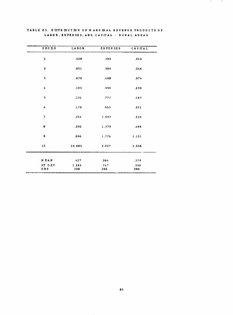
TABLE B3. DISTRIBUTION OF MARCGINAL REVENUE PRODUCTS OF

LABOR, EXPENSES, AND CAPITAL - RURAL AREAS

DECILE LABOR EXPENSES CAPITAL

1 .028 .302 .016

2 .051 .386 .046

3 .070 .468 .074

4 .103 .596 .130

5 .131 .777 .167

6 .179 .953 .221

7 .251 1.097 .310

8 .390 1.379 .499

9 .896 1.776 1.101

10 16.085 5.007 3.358

M EAN .427 .964 .379

ST DEV 1.183 .747 .556O R S 288 288 288

83

Bibliography

Althaus. Jaime, and Jorge Morelli (1980). Approximaciones a La Composicion v Evolucion del EmpleoInformal en El Peru. Lima: Pontificia Universidad Catolica del Peru, Mimeo.

Babb, Florence E. (1984). 'Women in the Marketplace: Petty Commerce in Peru." Review of RadicalPolitical Economics 16(1): 45-59.

Bates, D.M., and D.G. Watts (1980). "Relative Curvature Measures of Nonlinearity (with discussion)."Journal of the Roval Statistical Societv B 42: 1-25.

Belsey, David A., Edwin Kuh, and Roy E. Welsch (1980). Regression Diagnostics: Identifving InfluentialData and Sources of Coilinearitv. New York: Wiley.

Bromley, Ray (1978). "The Urban Informal Sector: Why is It Worth Discussing?" World Development 6,9/10, 1033-1039.

Buvinic Mayra, Margaret A. Lycette, and William Paul McGreevey (1983). Women and Povertv in theThird World. Baltimore: The Johns Hopkins University Press.

Bunster, Ximena, and Elsa Chaney (1985). Sellers and Servants: Working Women in Lima. New York:Praeger Press.

Chatterjee, Samprit, and Ali S. Hadi (1988). Sensitivitv Analvsis in Linear Regression. New .'ork: Wiley.

Chiswick, Carmel U. (1983). "Analvsis of Earnings from Household Enterprises: Methodology andApplication to Thailand." Review of Economics and Statistics LXV: No. 4, November, 656-662.

Cornia, Giovanni A., Richard Jollv. and Frances Stewart, eds. (1987). Adjustment with a FHiuman Face:Protecting the Vulnerable and Promoting Growth. Oxford: Clarendon Press.

Cornia, Giovanni A. (1987). "Adjustment at the Household Level: Potentials and Limitations of SurvivalStrategies." In Giovanni A. Cornia, Richard Jolly, and Frances Stewart, eds. Aditjstinent with a HumanFace: Protecting the Vulnera;,e and Promoting Growth. Oxford: Clarendon Press.

de Soto, Hernando (1988). The Other Path: The Invisible Revolution in the Third World. New York:Harper and Row. (First published in Spanish in 1986 as El Otro Sendero: La Revolucion Informal. Lima:Editorial El Barranco.)

Freeman, Donald B., and Glen B. Norcliffe (1985). Rural Enterprise in Kenva: Development and SpatialOrganization of the Nonfarm Sector. Chicago: University of Chicago, Department of Geography, ResearchPaper No. 214.

Gle±wwe, Paul, and Dennis de Tray (1989). The Poor in Latin America During Adjustment: A Case Studvof Peru. Washington, D.C: The W'orld Bank, Population and Human Resources Department, Welfare andHuman Resources Division, Living Standards Measurement Study Working Paper No. 24.

Grootaert, Christiaan, and Ana-Maria Arriagada (1986). 'rhe Peru Living Standards Survev: An AnnotaiedQuestionnaire. Washington, D.C: The World Bank, Development Research Department, Living StandardsMcasurement Study Working Paper Number 24.

84

Hallak. Jacques. and Francoise Caillods (1981). Education, Trainine and the Traditional Sector. Paris:UNESCO.

Hart, Keith J. (1987). "Informal Economy." In John Eatwell, Murray Milgate, and Peter Newman, eds. TheNew Paigrave: A Dictionarv of Economics. London: The MacMillan Press, 845-46.

Hart, Keith J. (1973). "Informal Income Opportunities and Urban Employment in Ghana." Journal ofModern African Studies 11: No. 1, 61-89.

Herz, Barbara (1989). "Bringing Women into the Economic Mainstream" Finance & Development 32: No.4, December, 22-25.

House, William J. (1984). "Nairobi's Informal Sector: Dynamic Entrepreneurs or Surplus Labor?" EconomicDevelopment and Cultural Change 32: No. 2, 277-302.

Instituto Nacional de Estadistica, INE (1988). Encuesta Nacional de Hogares Sobre Medicion de Nivelesce Vida Enniv (1985-86): Analisis de Resultados. Lima: INE.

Inter-American Development Bank, IDB, (1988). Ten Years of Small Projects: Bringine the Marein intothe Mainstream. Washington, D.C: IDB.

Inter-American Development Bank, IDB, (1988). Annual Report, 1988. Washington, D.C: IDB.

Inter-American Development Bank, IDB, (1987a). Biblioeraphv on the Urban Informal Sector. Washington.D.C: Plans and Programs Department, Social Policies Division, IDB.

Inter-American Development Bank, IDB, (1987b). Economic and Social Progress in Latin America: 1987Report. Washington, D.C: IDB.

International Labour Office (1972). Emplovment Incomes and Equalitv: A Stratevv for Increasing ProductiveEmplovment in Kenva. Geneva: ILO.

Kafka, Folke (1984). El Sector Informal Urbano en la Economia Peruana. Lima: Centro de Investigacion,Universidad del Pacifico.

Litan, Robert, Luis Morales-Bayro, and Jorge Fernandez-Baca (1986)."Internal Structural Reforms in Peru:A Promising Road out of the Debt Crisis." Journal of Economic Growth 1: No. 2, 28-36.

Mazumdar, Dipak (1976). "'The Urban Informal Sector." World Development 4: No. 8, 655-679.

Mescher, Micheline (1985). The Urban Informal Sector in Latin America: Case Studies of Peru and Brazil.Alexandria, Va.: Mescher Associates.

Mattera, PLilip (i985). Off the Books: The Rise of the UnderEground Economv. New York: St. Mattin'sPress.

Moock, Peter, Philip Musgrove, and Morton Stelcner, (1989). Education and Earnings in Peru's InformalNonfarm Familv Enterprises. Washineton, D.C.: Population and Human Resources Department, Educationand Emplovment Division, Policy, Planning and Research Complex, WPS 236.

Moser, Caroline 0., and Judith Marsie-Hazen (1984). A Survev of Empirical Studies in Industrial andManufacturing Activities in the Informal sector in Dcvelopinf-g Countries. New York: UNIDO.

85

OECD - Organisation for Economic Co-operation and Development (1989). Development Co-operationin the 1990s: Efforts and Policies of the Members of Ihe Development Assistancc Committee: Paris, OECD.

PREALC - program regional de empleo en America Latina y el Caribe (1985). Mas Alla de la Crisis.Santiago, Chile: PREALC.

Racine, Jeffrey S. (1989). A Semiparametric Approach to the Estimation of Svstems of Equations Modelsin the Presence of Heteroskedasticitv of Unknown Form. Toronto: Department of Economics, YorkUniversity Working Paper 89-13.

Reichmuth, Markus (1978). Dualism in Peru: An Investigation into the Inter-relationships between Lima'sInformal Clothing Industrv and the Formal Sector. Oxford: B. Litt. thesis, Oxford University.

Ross, W.H. (1987). "The Geometry of Case Deletion and the Assessment of Influence in NonlinearRegression." Canadian Journal of Statistics 15: 91-103.'

Schafgans. Marcia (1989). The Status of Women in the Economv of Peru: A Descriptive Analvsis.Washington D.C: The World Bank, Population and Human Resources Department, Women in DevelopmentDivision, (unpublished manuscript).

Sethuraman S.V. ed. (1981). The Urban Informal Sector in Developing Countries: Emplovment. Povertvand Environment. Geneva: ILO.

Stewart, Frances (1987). "Supporting Productive Emplovment Among Vulnerable Groups." In GiovanniAndrea Cornia, Richard Jollv, and Frances Stewart, eds. Adjustment with a Human Face: Protecting theVulnerable and Promoting Growth. Oxford: Oxford University Press.

Strassmann, Paul, W. (1987). "Home-based Enterprises in Cities of Developing Countries." EconomicDevelopment and Cultural Change 36: No. 1, 121- 144.

Stelcner. Morton, and Peter Moock (1988). Nonagricultural Familv Enterprises in Peru: The Role of theInformal Sector in a Developing Economv. Washington, D.C: The World Bank, Population and HumanResources Department, Welfare and Human Resources Division, (unpublished manuscript).

Suarez-Berenguela, Ruben M. (1987). Peru Informal Sector, Labor Markets, and Returns to Education.Washington, D.C: The World Bank,Development Research Department, Living Standards MeasurementStudy, No. 41.

Tendler, Judith (1983). Ventures in the Informal Sector and How Thev Worked Out in Brazil. AIDEvaluation Special Studv No. 12. Washington, D.C.: Agency for International Development.

Tinker. Irene (1987). "Street Foods: Testing Assumptions About Informal Sector Activity by Women andMen." Current Sociology 35, Winter, 1-81.

Tokman, Victor (1986). "Adjustment and Employment in Latin America." International Labour Review125: No. 5.

Tokman, Victor (1978). "An Exploration into the Nature of Formal-Informal Sector Relationships.' WorldDevelopment 6: No. 9-10, 1065-75.

86

Ullah, Aman (1988). "Non-parametric Estimation of Econometric Functionals." Canadian Journal ofEconomics 20: No. 3. 625-58.

United Nations (1985). Bank Credit for Rural Women: Report on Study Tour of Grameen Bank inBangladesh. Bangkok: Economic and Social Commission for Asia and the Pacific.

van der Gaag, Jacques, Morton Stelcner, and Wim Vijverberg (1989). 'Wage Differentials and Moonlightingby Civil Servants: Evidence from Cote d'lvoire and Peru." The World Bank Economic Review 5: No. 3,67-98.

Vargas-Llo. ±, Mario (1987). "The Silent Revolution." Journal of Economic Growth 2: No. 1, 3-7.

Webb, Richard C. (1977). Government Policv and the Distribution of Income in Peru: 1963-1973.Cambridge, Mass.: Harvard University Press.

World Bank (1989). World D±!velopment Report. New Yorkc Oxford University Press and the World Bank.

World Bank (1987). WolId Development Report. New York: Oxford University Press and the World Bank.

87

PRE Working Paper Series

ContactAuigho for paper

WPS444 The Political Economy of Inflation Stephan Haggard June 1990 A. Oropesaand Stabilization in Middle-Income Robert Kaufman 39176Countries

WPS445 Pricing, Cost Recovery, and Rachel E. Kranton June 1990 W. WrightProduction Efficiency in Transport: 33744A Critique

WPS446 MEXAGMKTS: A Model of Crop Gerald T. O'Mara July 1990 C. Spoonerand Livestock Markets in Mexico Merlinda lngco 30464

WPS447 Analyzing the Effects of U.S. Gerald T. O'Mara July 1990 C. SpoonerAgricultural Policy on Mexican 30464Agricultural Markets Using theMEXAGMKTS Model

WPS448 A Model of U.S. Corn, Sorghum, Richard E. Just July 1990 C. Spoonerand Soybean Markets and the 30464Role of Government Programs(USAGMKTS)

WPS449 Analysis of the Effects of U.S. Richard E. Just July 1990 C. SpoonerMacroeconomic Policy on U.S. 30464Agriculture Using the USAGMKTSModel

WPS450 Portfolio Effects of Debt-Equity Daniel Oks June 1990 S. King-WatsonSwaps and Debt Exchanges 31047with Some Applications toLatin America

WPS451 Productivity, Imperfect Competition Ann E. Harrison July 1990 S. Fallonand Trade Liberalization in 38009the C6te d'lvoire

WPS452 Modeling Investment Behavior in Nemat Shafik June 1990 J. IsraelDeveloping Countries: An 31285Application to Egypt

WPS453 Do Steel Prices Move Together? Ying Qian June 1990 S. LipscombA Cointegra n Test 33718

WPS454 Asset and Liability Management Toshiya Masuoka June 1990 S. Bertelsmeierin the Developing Countries: Modern 33767Financial Techniques -- A Primer

WPS455 A Formal Estimation of the Effect Junichi Goto June 1990 M. T. Sanchezof the MFA on Clothing Exports 33731from LDCs

PRE Working Paper Series

ContactIiS ~~~~~ ~ ~~Author DQ for paper

WPS456 Improving the Supply and Use of S. D. Foster June 1990 Z. VaniaEssential Drugs in Sub-Saharan Africa 33664

WPS457 Financing Health Services in Africa: Germano Mwabu June 1990 Z. VaniaAn Assessment of Alternative 33664Approaches

WPS458 Does Japanese Direct Foreign Kenji Takeuchi June 1990 J. EppsInvestment Promote Japanese Imports 33710from Developing Countries?

WPS459 Policies for Economic Development Stanley Fischer June 1990 WDR OfficeVinod Thomas 31393

WPS460 Does Food Aid Depress Food Victor Lavy July 1990 A. Murphyf roduction? The Disincentive 33750Dilemma in the African Context

WPS461 Labor Market Participation, Returns Shahidur R. Khandker July 1990 B. Smithto Education, and Male-Female 35108Wage Differences in Peru

WPS462 An Alternative View of Tax Anwar Shah July 1990 A. BhallaIncidence Analysis for Developing John Whalley 37699Countries

WPS463 Redefining Government's Role in Odin Knudsen August 1990 K. CabanaAgriculture in the Nineties John Nash 37946

WPS464 Does A Woman's Education Affect Shoshana Neuman August 1990 V. CharlesHer Husband's Earnings? Results Adrian Ziderman 33651for Israel in A Dual Labor Market

WPS465 How Integrated Are Tropical Timber Panos Varangis August 1990 D. GustafsonMarkets? 33714

WPS466 Is There An Intra-Household Lawrence Haddad August 1990 J. SweeneyKuznets Curve? Ravi Kanbur 31021

WPS467 Structural Adjustment and Living Nanak Kakwani August 1990 B. RosaConditions in Developing Countries Elene Makonnen 33751

Jacques van der Gaag

WPS468 Does the Structure of Production Indermit Gill August 1990 M. AbundoAffect Demand for Schooling in Peru? 36820

WPS469 Modeling Economic Behavior in J. Barry Smith August 1990 M. AbundoPeru's Informal Urban Retail Sector Morton Stelcner 36820