Modeling Downturn LGD for a Retail Portfolio - … · 2011-02-19 · Kungliga Tekniska Hogskolan...
87
Kungliga Tekniska H ¨ ogskolan Modeling Downturn LGD for a Retail Portfolio Author: Andreas Wirenhammar January 2010
Transcript of Modeling Downturn LGD for a Retail Portfolio - … · 2011-02-19 · Kungliga Tekniska Hogskolan...
Kungliga Tekniska Hogskolan
Modeling Downturn LGD for a RetailPortfolio
Author:
Andreas Wirenhammar
January 2010

Modeling Downturn LGD for a Retail Portfolio
By: A. Wirenhammar 2

Abstract
Loss given default is a very important measure in credit risk. This measure however might be
affected by the state of the econonomy, especially in downturn conditions. The Basel II accord
requires financial institutions to calculate the expected loss for their credit portfolio in downturn
conditions. As a part of this, downturn loss given default has to be estimated. The Swedish
FSA define downturn conditions as the conditions during the 90s crisis. This leads to the need
to create a model for quantifying the loss given default factor during downturn conditions. The
modeling is complicated by the lack of saved data from this period. This paper will discuss
numerous different approaches on how to solve this problem and as we will see, most approaches
do not give any reasonable results with our dataset. Instead this paper recommends a multifactor
model to be used until sufficient data have been amassed.
By: A. Wirenhammar 3

Modeling Downturn LGD for a Retail Portfolio
By: A. Wirenhammar 4

Sammanfattning
Forlust givet konkurs ar ett mycket viktigt matt inom kreditrisk. Detta matt ar dock inte kon-
stant utan kan paverkas av saker sa som ekonomins tillstand, speciellt under recessioner. Basel
II kraver att finansiella institut beraknar forvantade forluster for sin kreditportfolj i en recession-
speriod. Som en del i detta maste recessionsforlust fororsakad av konkurs (EN:Downturn Loss
Given Default) skattas. Finansinspektionen definierar recession i det har sammanhanget som
det tillstand som radde under nittiotalskrisen. Det har leder till behovet att kvantifiera forlust
fororsakad av konkurs under dessa forhallanden. Denna modellering kompliceras av bristen pa
data fran nittiotalskrisen. Den har uppsatsen diskuterar flera olika satt att komma runt denna
problematik men vi kommer att se att de flesta modeller inte ger nagra rimliga resultat. Istallet
rekommenderas en linjar multifaktormodell tills dess att en storre datamangd samlats in.
By: A. Wirenhammar 5

Modeling Downturn LGD for a Retail Portfolio
By: A. Wirenhammar 6

Acknowledgements
Firstly I would like to thank my supervisor at the Royal Institute of Technology, Harald Lang
and my supervisor at Nordea Gustaf Stael von Holstein for their feedback and advise. I would
also like to thank Olof Stangenberg, Fredrik Eriksson and Alexander Kamoun at Nordea for
practical help.
Moreover I would like to thank Ann-Charlotte Kjellberg for helping me with SAS and Torbjorn
Isaksson for access to time series of macro data in EcoWin. I would also like to thank my father
Sven and my brother Markus for helping me proof read this thesis.
By: A. Wirenhammar 7

Modeling Downturn LGD for a Retail Portfolio
By: A. Wirenhammar 8

Contents
1 List of Abbreviations 11
2 Introduction 13
2.1 Background . . . . . . . . . . . . . . . . . . . . . . . . . . . . . . . . . . . . . . . 13
2.2 Scope . . . . . . . . . . . . . . . . . . . . . . . . . . . . . . . . . . . . . . . . . . 14
2.3 Method . . . . . . . . . . . . . . . . . . . . . . . . . . . . . . . . . . . . . . . . . 14
2.4 Purpose . . . . . . . . . . . . . . . . . . . . . . . . . . . . . . . . . . . . . . . . . 15
2.5 Hypothesis . . . . . . . . . . . . . . . . . . . . . . . . . . . . . . . . . . . . . . . 15
3 Theoretical Background 17
3.1 Basel II . . . . . . . . . . . . . . . . . . . . . . . . . . . . . . . . . . . . . . . . . 17
3.2 Probability of Default . . . . . . . . . . . . . . . . . . . . . . . . . . . . . . . . . 18
3.3 Loss Given Default . . . . . . . . . . . . . . . . . . . . . . . . . . . . . . . . . . . 18
3.4 Credit Conversion Factor . . . . . . . . . . . . . . . . . . . . . . . . . . . . . . . 19
3.5 Risk Weighted Assets . . . . . . . . . . . . . . . . . . . . . . . . . . . . . . . . . 21
3.6 Previous research . . . . . . . . . . . . . . . . . . . . . . . . . . . . . . . . . . . . 22
3.7 What does ”downturn” mean? . . . . . . . . . . . . . . . . . . . . . . . . . . . . 23
3.8 What characterized the Swedish property crisis . . . . . . . . . . . . . . . . . . . 24
3.9 Downturn LGD . . . . . . . . . . . . . . . . . . . . . . . . . . . . . . . . . . . . . 26
4 Data 29
5 Models 31
5.1 Multiplicative Factor Model . . . . . . . . . . . . . . . . . . . . . . . . . . . . . . 32
5.2 Copulas . . . . . . . . . . . . . . . . . . . . . . . . . . . . . . . . . . . . . . . . . 33
By: A. Wirenhammar 9

Modeling Downturn LGD for a Retail Portfolio
5.3 Latent variable single factor model . . . . . . . . . . . . . . . . . . . . . . . . . . 34
5.4 Regression models . . . . . . . . . . . . . . . . . . . . . . . . . . . . . . . . . . . 39
5.4.1 Macroeconomic Drivers, Previous Research . . . . . . . . . . . . . . . . . 39
5.4.2 Macroeconomic factors . . . . . . . . . . . . . . . . . . . . . . . . . . . . . 40
5.4.3 Time Lags . . . . . . . . . . . . . . . . . . . . . . . . . . . . . . . . . . . . 41
5.4.4 Macroeconomic Drivers . . . . . . . . . . . . . . . . . . . . . . . . . . . . 42
5.4.5 Non Macro Drivers . . . . . . . . . . . . . . . . . . . . . . . . . . . . . . . 47
5.4.6 Regression . . . . . . . . . . . . . . . . . . . . . . . . . . . . . . . . . . . . 49
5.4.7 OLS . . . . . . . . . . . . . . . . . . . . . . . . . . . . . . . . . . . . . . . 49
5.5 Linear Multifactor Model . . . . . . . . . . . . . . . . . . . . . . . . . . . . . . . 50
5.6 Microdata Model . . . . . . . . . . . . . . . . . . . . . . . . . . . . . . . . . . . . 51
6 Results 55
6.1 Regression models . . . . . . . . . . . . . . . . . . . . . . . . . . . . . . . . . . . 55
6.2 Linear Multifactor Model . . . . . . . . . . . . . . . . . . . . . . . . . . . . . . . 59
6.3 Latent Variable Single Factor Model . . . . . . . . . . . . . . . . . . . . . . . . . 59
7 Conclusion 61
Appendices 65
A Table over macro data sources 67
B Plots of macro data 71
C Pool Specification 85
D Alternative Regressions 87
By: A. Wirenhammar 10

Chapter 1
List of Abbreviations
AIRB - Advanced Internal Rating Based
CCF - Credit Conversion Factor
DCCF - Downturn Credit Conversion Factor
DLGD - Downturn Loss Given Default
EAD - Exposure at Default
EL - Expected Loss
FRIB - Foundation Internal Rating Based
FSA - Financial Supervisory Authority
LGD - Loss Given Default
PD - Probability of Default
RWA - Risk Weighted Assets
SME - Small and Medium Enterprises
UL - Unexpected Loss
By: A. Wirenhammar 11

Modeling Downturn LGD for a Retail Portfolio
By: A. Wirenhammar 12

Chapter 2
Introduction
The Theoretical Background section below will go through a number of terms and definitions
that are needed to get this section well defined. Any reader not familiar with the area is strongly
recommended to read the Theoretical Background before reading this section.
2.1 Background
A bank is a very complex environment that have many different types of risk that must be
handled such as credit risk, market risk and operational risk. There are several reasons for this,
firstly to be able to make a profit, losses due to risk must be handled. Secondly the government
and society at large also has an interest to limit risk in banks and other financial institutions.
This due to the systemic effects if a financial actor goes into bankruptcy due to excessive risk
taking. An example of this is Lehman Brothers which took excessive risk, the market went
against them and thus they went into bankruptcy. This led to that all the liquidity in the
financial system dried up overnight, since no one knew if anyone else was sitting on toxic assets.
This caused major disrutions in the world economy and the effects can still be felt. To avoid this
from happening, banks are required to have a certain amount of capital that can absorb losses
so that the bank can avoid to go into bankruptcy if things goes bad.
The Basel II Accord, initially published 2004, is an international recommendation on banking
laws and regulations and as such they discuss the subject of required capital thoroughly. The
By: A. Wirenhammar 13

Modeling Downturn LGD for a Retail Portfolio
Basel II accord has three pillars:
• The first pillar deals with the required capital for credit risk, market risk and operational
risk.
• The second pillar deals with how the regulating authority should deal with the require-
ments in pillar one and also discusses how other risks such as legal risk, systemic risk and
concentration risk should be handled.
• The third pillar requires banks to publish certain information about their risk management,
this to promote stability in the system.
2.2 Scope
The scope of this paper is to look at a method that can be used by Nordea for calculating
downturn LGD for both internal use and to be used in the capital requirement calculations.
This paper will not discuss how to calculate downturn PD and therefore refer interested readers
to existing extensive academic research already performed in the area. The reason for excluding
PD is to limit the amount of work.
This paper is limited to use Nordea’s internal data on the retail portfolio and data that is publicly
available. For more through description of the data and its scope, please see the Data section
below.
We also limit this to models that are based on some kind of data. While purely theoretical
models might be interesting, it is hard to corroborate from a economic perspective why they
should be able to predict the downturn LGD in real scenarios.
This means that this paper will only look at the downturn scenarios, while calculating the
variables in a normal (non-downturn) scenario is outside the scope of this paper.
2.3 Method
This paper will go through a number of different modeling paradigms and discuss if and why are
feasible to use. If we are able to use the model and our data to predict a downturn LGD value
By: A. Wirenhammar 14

Modeling Downturn LGD for a Retail Portfolio
we will do so and discuss from an economic perspective if the result is reasonable.
This means that the work on this essay will be split into two distinctive parts. First we will
perform a thorough literature study to find good models. In the second phase we will test these
models with our dataset.
2.4 Purpose
The purpose of this paper is to find a way to model the downturn LGD factor in a way that is
both mathematically correct and that is acceptable for FSA. The model will mainly be used to
improve Nordea’s internal calculations of these factors, due to new internal demand on develop-
ment.
A requirement is that the model must be able to stress the LGD with a crisis scenario like the
1990’s crisis.
2.5 Hypothesis
The hypothesis is that the LGD for the retail portfolio is not significantly affected by an eco-
nomic downturn. I.e. LGD≈DLGD. The intuition for this is the fact that defaults by physical
person’s carries severe consequences in all the Nordic countries, hence obligors in distress will
try everything before defaulting. Default of a physical person does not mean that the loans are
written off like in the case of a juridical person. Since the retail portfolio consists mainly of
mortgages to physical persons for which the bank has both good collaterals covering the loan
and obligors with high motivation to avoid default.
By: A. Wirenhammar 15

Modeling Downturn LGD for a Retail Portfolio
By: A. Wirenhammar 16

Chapter 3
Theoretical Background
3.1 Basel II
The Basel II accord is a collection of recommendations on banking laws and financial regulations
issued by the Basel Committee on Banking Supervision. The purpose with these recommenda-
tions is to create standards regarding how much capital a bank needs to hold against financial
risk and other types of risk.[1][paragraph 1,4]
To decide the capital that a financial institution need to hold against credit risk one must calculate
expected loss (EL) and unexpected loss (UL), where EL is seen as a cost of doing business and
UL represents the potential for unexpected losses.
Figure 3.1
By: A. Wirenhammar 17

Modeling Downturn LGD for a Retail Portfolio
[3]
EL is calculated by the formula:
EL = PD ∗ LGD ∗ EAD (3.1)
Were PD is probability of default, LGD is loss given default and EAD is exposure at de-
fault.
3.2 Probability of Default
Probability of Default (PD) is the probability that an obligor will default over a period of one
year. A lot of research has been done on how this factor should be modeled and stressed.
One reason for this might be that in the FIRB the banks are only required to estimate PD
themselves.
3.3 Loss Given Default
Loss given default (LGD) is defined as the credit loss that is incurred if an obligor defaults
expressed as a percentage of the exposure at default.[1]
According to the Basel II accord AIRB approach, a bank’s estimation of LGD may not be lower
than the historical long run default weighted average. This is can be calculated as:
LGD = 1− EAD +∑
(NPV(Increases))−∑
(NPV(Decreases))
EAD(3.2)
cashflows after the default is discounted back to the time of the default using a interest rate
that takes the risk and uncertainty of the cashflows into account. This method is based on the
statement:
”When recovery streams are uncertain and involve risks that cannot be diversified away, net
present value calculations must reflect the time value of money and a risk premium appropriate
to the undiversifiable risk.”[1][paragraph 468]
By: A. Wirenhammar 18
Modeling Downturn LGD for a Retail Portfolio
The quote is extracted from the Guidance on Paragraph 468 of the Framework Document by the
Basel Committee on Banking Supervision.
This discount rate can be determined in many ways and one example is using the rate on
government bonds and adding a risk premium. Others have tried to calculate the correct rate
backwards by using the price of defaulted publicly traded bonds before and after default and the
actual recoveries, to determine which rate this implies.[26]
In addition to these criteria the bank also has taken into account that the LGD may be higher dur-
ing an economic downturn. This is taken into account by calculating a downturn LGD.[1][paragraph
468] How this should be done is however not defined in the accord.
3.4 Credit Conversion Factor
Exposures can be split in two categories, on balance and off balance. On balance means that
some kind of exposure they is included in the balance sheet. An example of this is a mortgage.
Off balance means items that are not currently on the balance sheet but which could lead to
items on the balance sheet in the future.. An example of this is a mortgages in principle (SV:
lanelofte.) This means that the bank promise to lend money to a prospective homebuyer if he
buys anything within a specified time period, this could lead to a loan that ends up on the
balance sheet and is thus classified as off balance. For the on balance the entire amount of the
exposure is used in the capital calculation. In the case of off balance exposures however capital
must only be held against a part of the exposure. This part is calculated by multiplying the off
balance with a credit conversion factor (CCF). This factor should capture how much of the off
balance that has been utilized at the time of default.[1][paragraph 82]
By: A. Wirenhammar 19

Modeling Downturn LGD for a Retail Portfolio
Exposure
Committed amount
Exposure
Time
Utilized amount Off Balance*CCF
Off Balance
On Balance
Time of Default Measurement point, t=0
Figure 3.2
Exposure at default (EAD) can thus be calculated using the formula:
EAD = On Balance + CCF ∗Off Balance (3.3)
[1][paragraph 308-310]
If the equations 3.3 is solved for CCF we get:
CCF =EAD−On Balance
Off Balance(3.4)
Where the on balance and off balance are known quantities but the CCF factor must be calculated
using historical data. According to the Basel II accord banks must take into account that the
CCF factor might be higher during an economic downturn.[1][paragraph 474-479] This is done
by calculating a downturn CCF factor and test if it deviates from the average historical CCF
factor.
The Basel II accord can be interpreted to support the view that the CCF must be expressed in
this way. The EU implementation of the Basel II, the Capital Requirements Directive (CRD),
implicitly states that the CCF factor must be higher than zero.[5][p 81]
The CCF factor is called Loan Equivalent (LEQ) or Usage Given Default (UGD) in some litera-
ture. Some American literature even defines the term CCF differently than we do and use one of
By: A. Wirenhammar 20
Modeling Downturn LGD for a Retail Portfolio
the above terms for what we would call CCF.[5][p 81] In this paper however only the definition
in equation 3.4 is used.
3.5 Risk Weighted Assets
Risk weighted assets (RWA) is given by the formula:
RWA = K ∗ 12.5 ∗ EAD (3.5)
Where K is the capital requirement. K is given by different formulas for different asset classes.
For retail the formula is:
K = LGD ∗ Φ[(1−R)−0.5 ∗ Φ−1(PD) +
(R
1−R
)0.5
∗ Φ−1(0.9999)]− PD ∗ LGD (3.6)
This formula is derived from an Asymptotic Single Risk Factor (ASRF) model. This means that
we model the loss rate as only dependant on a single factor and that the individual idiosyncratic
risk factors of individual exposure do not have any effect. The reasons for choosing this model
is that the Basel Committee wanted a portfolio invariant measure, i.e. only the characteristics
of the new loan should matter. There should be no marginal effects based on the portfolio it is
added to. One of the reasons for this is that it would be difficult for the employees in the branch
network to know how they are supposed to run their business if the conditions changes because
of the portfolio. It would be even hard to explain to the costumer why the loan they were as
good as promised last week can not be done suddenly. The demand for a portfolio invariant
model more or less limited the choice to an ASRF model. [4]
The term Φ−1(PD) in the equation above represents the default threshold and the (1− R)−0.5
factor is a penalty based on the default correlation R. The Φ−1(0.9999) term represents a con-
servative value of the systematic risk factor and(
R1−R
)0.5
is a penalty based on the default
correlation R.
The correlation R in the capital requirement formula above is set to 0.15 for retail mortgages
by the Basel II Accord. The formula for qualifying revolving credit facilities is the same with
the difference that R=0.04. Retail exposure not covered by these two categories uses the for-
mula:
By: A. Wirenhammar 21

Modeling Downturn LGD for a Retail Portfolio
R = 0.03
[1− exp(−35 ∗ PD)
1− exp(−35)
]+ 0.16
[1− (1− exp(−35 ∗ PD)
1− exp(−35)
](3.7)
to calculate R.[1][paragraph 328] This formula gives a correlation between 3% (when PD=1) and
16% (when PD=0). The factor 35 decides how fast the correlation decreases when PD decreases
and the choice of 35 here mean that the decline is slower than the equivalent case for corporate
where it is set to 50.
The Basel II accord has three different approaches to measure credit risk: Standardized, Foun-
dation Internal Rating Based (FIRB) and Advanced Internal Rating Based (AIRB).
If using the standardized approach the banks are required to use the credit ratings of an external
credit rating agency to quantify the required amount of capital.
The banks using the FIRB approach are allowed to quantify their own PDs but are required to
use the regulators LGD and banks using the AIRB approach are allowed to estimate their own
PDs, EADs and LGDs.
In general the AIRB requires less capital than FIRB and FIRB requires less capital than the
standardized approach. This since the more advanced methods only can be used if the bank has
sufficient historical data. This means that the bank can replace conservative estimations with
historical values that in general show less credit losses than the conservative estimations.
3.6 Previous research
When Basel II was implemented, both financial institutions and researchers focused on how to
estimate PD. As when some improvements had been discovered focus shifted to LGD. This means
that in the case of LGD, a comparison of model suitability can conducted and subsequently tested
with data.
While there have been numerous studies modeling downturn LGD, most of these have focused
on corporate credit portfolios, mainly publicly traded bonds. The reason for this is simple, data
on and about corporation issuing public bonds is easily available and market values of publicly
traded bonds are readily available.
The Vasieck model used in the Basel II accord does not take the correlation between LGD and
PD into account. This has lead to a large number of researchers trying to correct this, by
By: A. Wirenhammar 22

Modeling Downturn LGD for a Retail Portfolio
suggesting models that take this correlation into account. The largest group of such models is
the factor models group. This group of models assumes that both PD and LGD are driven by
some kind of common latent variable. An example of this kind of model is Frey 2000 with one
systematic and one idiosyncratic factors , Hillebrand 2006 two systematic factors, Barco 2007
with two systematic factors and Chabane Laurent and Salomon with two systematic and two
idiosyncratic factors.
There are also attempts to model downturn LGD with copulas and an example of this is Hui Li
2010 which discusses a copula model for only two loans but which could theoretically be extended
to any number of loans.
Others, such as Chalupka et al 2008, discuss numerous simpler models. Most of these however
are not relevant since they are not based on data or are based on data that are not available.
Ozdemir and Miu 2009 suggest three approaches of which two will be tested in this paper, namely
stress LGD by macro factors and a PD-LGD correlation model. A good example of an article
building of a macro-stressable model is Caselli et al 2008 which comes to the conclusion that
three macro factors are the main determinants for LGD.
Another interesting approach is to model LGD based on micro-data such as employment status,
income, marriage, etc for each obligor. This has been done by Belloti and Cook 2009 and this
kind of model is also supported by Roszbach at Riksbanken. This kind of data is not available
to the author and will thus not be explored in this paper. Basing a model on this type of data
and changing the status of people, for example from employed to unemployed, would probably
be a very good model for downturn LGD and further research in the area should be done as data
become available.
3.7 What does ”downturn” mean?
An important aspect of this task is to determine how to define ”downturn”. According to the
Swedish FSA there are no periods during the twenty-first century that can be seen as downturns
in this regard.[8][p 12] This guideline was however published in 2007, i.e. before the financial
crisis. While one could argue that the recent financial crisis was severe enough, the credit losses
for Swedish banks have not been significant if we disregard the Baltic exposures. An example of
this is that for private persons in Sweden that were not laid off, there has been no crisis at all.
By: A. Wirenhammar 23
Modeling Downturn LGD for a Retail Portfolio
Instead they have experienced lowered taxes and extremely low interest rates. Since this paper
is based on data from Nordea’s retail portfolio in the Nordic countries we have to look at another
crisis. This implies that the best period to look at is the years during the nineties crisis. This is
in line with the FSA that states that
”...the nineties can give good guidance on how such a (downturn) period might look.” [8][p 12]
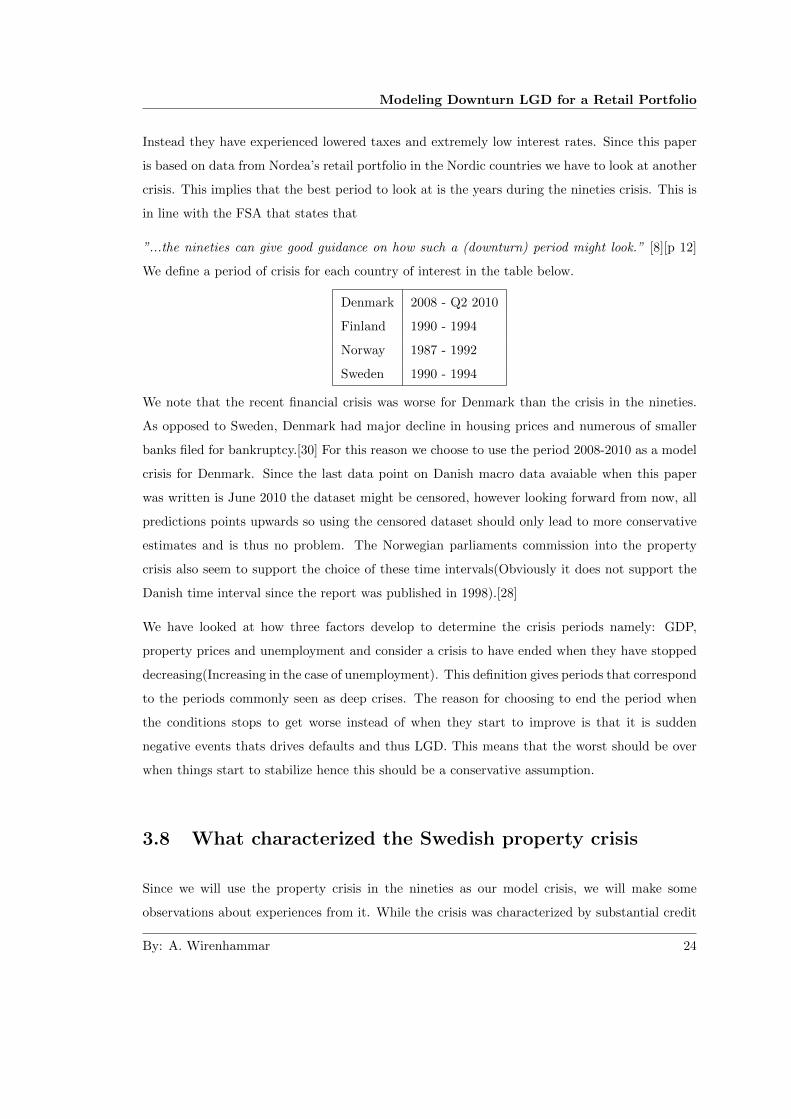
We define a period of crisis for each country of interest in the table below.
Denmark 2008 - Q2 2010
Finland 1990 - 1994
Norway 1987 - 1992
Sweden 1990 - 1994
We note that the recent financial crisis was worse for Denmark than the crisis in the nineties.
As opposed to Sweden, Denmark had major decline in housing prices and numerous of smaller
banks filed for bankruptcy.[30] For this reason we choose to use the period 2008-2010 as a model
crisis for Denmark. Since the last data point on Danish macro data avaiable when this paper
was written is June 2010 the dataset might be censored, however looking forward from now, all
predictions points upwards so using the censored dataset should only lead to more conservative
estimates and is thus no problem. The Norwegian parliaments commission into the property
crisis also seem to support the choice of these time intervals(Obviously it does not support the
Danish time interval since the report was published in 1998).[28]
We have looked at how three factors develop to determine the crisis periods namely: GDP,
property prices and unemployment and consider a crisis to have ended when they have stopped
decreasing(Increasing in the case of unemployment). This definition gives periods that correspond
to the periods commonly seen as deep crises. The reason for choosing to end the period when
the conditions stops to get worse instead of when they start to improve is that it is sudden
negative events thats drives defaults and thus LGD. This means that the worst should be over
when things start to stabilize hence this should be a conservative assumption.
3.8 What characterized the Swedish property crisis
Since we will use the property crisis in the nineties as our model crisis, we will make some
observations about experiences from it. While the crisis was characterized by substantial credit
By: A. Wirenhammar 24

Modeling Downturn LGD for a Retail Portfolio
losses for most banks, most of the credit losses came from corporate exposures. Credit losses
from private persons were comparably small. The loans to private individuals represented 2%
of credit losses in 1992. In 1993 this hade increase to 26% of losses and was 23% in 1994.
In money the amounts where 385 MSEK 1992, 1098 MSEK 1993 and 500 MSEK 1994. The
large increase private persons share in total loan losses can partly be explained by the transfer
of assets to Securum in 1993. The transfered assets where mainly non performing corporate
loans meaning that it changed the portfolio composition, this however can not explain the whole
increase. [14][15][16]
There are several reasons for this, firstly the most common reason that private persons default is
sudden unemployment or sickness. In many cases these are temporary conditions and default can
be handled by simply lowering amortization until the person gets a new job/recovers. Secondly,
residential mortgages have the residence as collateral, and in the few cases where the residence
is actually sold, the proceedings from the sale covers most of the debt. This means that any
remaining debt probably can be repaid by the obligor’s salary. This was true even during the
crisis.[31]
In the cases where the property did not cover most of the debt, the collateral was mainly very
remote houses that are problematic to sell, however in those cases the property did not cost
the defaulted that much either. The main category of private persons that defaults and leads
to actual losses is SME owners that have guaranteed their firm’s loans with private property.
Unfortunately the loan losses above can not be separted into losses on residential mortgages and
losses due to SME faliure.
It is also important to note that the crisis was caused by a number of structural changes. Since
then, people have either become accustomed to the changes or further changes have been made.
This means that the economy, regulations and the banks have changed since.[31] Firstly, during
the eighties the credit market in Sweden was de-regulated. Before this, the bank was only allowed
to increase net lending by a certain percentage each year. This led to a large unfilled demand for
credit by the households. When the market was de-regulated the households borrowed heavily,
quickly increasing their leverage. This at the same time as the banks accustomed to the regulation
did not have an adequate credit process in place. Secondly, until 1990 interest rates were fully
deductible in Sweden. This coupled with high marginal taxes on income made debts cheap
financing. During the beginning of the nineties there was a change from pegged currencies, and
full employment to floating currencies and inflation targeting, causing a major macro-economic
By: A. Wirenhammar 25

Modeling Downturn LGD for a Retail Portfolio
shift. However, it took time for the economy to adjust. The years after the change, interest
rates remained on the same nominal level as before, leading to a large increase in real interest
rate.[23]
Although it would have been interesting to investigate how the crisis in the nineties affected
the other Nordic countries, this has not been done due to the practical problems involved.
The differences however, should not be so large that the description above is an unreasonable
approximation even if it does not fit in every aspect. Especially in Denmark this might be an
issue since we use a total different time period for Denmark. All macro data used however, is
from the respective country.
3.9 Downturn LGD
There has been some research done into calculating LGD factors in downturn scenarios. This
research however focuses mostly on deriving purely theoretical models (as in no or very little
connection to real world data) or is based on publicly traded debt, almost always US corporate
bonds.[3] In the case of a traded bond one might see LGD as one minus the bond price after
default through the bond price before default. This however requires a market value, something
that is not available for mortgages. While this kind of research might be very interesting it is not
applicable without modification, since our model has to be based on real world data and market
prices are not available.
In general, many banks have problems calculating LGD and especially downturn LGD since they
lack sufficient data. There has been some research done on how to work around this problem.
Part of the solutions offered are the theoretical models mentioned above, and part are Monte
Carlo approaches or macro-economic models.
Chalupka et al state some approaches they think might be good ways to calculate downturn
LGD.[11] These are:
1. Use a different(read higher) discount factor
2. Work with default weighted LGD instead of exposure weighted or time weighted LGD
3. Take into the consideration the non-closed files, where the recovery is lower
4. Use macro-economic factors within several stress scenarios
By: A. Wirenhammar 26

Modeling Downturn LGD for a Retail Portfolio
5. Choose 5 worst years out of last 7 years
While 1. might partially serve to calculate downturn LGD, it clearly is not enough and impossible
given our dataset since the data only a single final LGD value is saved. Using only 1. disregards
several important factors. 2. are already done with the normal LGD so that would not change
anything. Currently, Nordea assumes that all recoveries are made within three years of the
default. Later recoveries are not considered. While 3. might imply an even shorter limit it does
not appear like a good way to estimate downturn LGD for several reasons. Most importantly
that it is a very subjective method and that it is not based on actual, accurate data. 4. is an
interesting approach which this paper will try to apply. 5. do not seem to capture a downturn
very well since if the last seven years have been good the result will be biased.
The methodology of picking the worst, might hold some value in some sense but for it to be
actually useful, it would have to be modeled differently. One might for example create a new
portfolio consisting of actual loans from the real portfolio but overweight the loans with high
LGDs. This might for example be done with the bootstrap method. While this methodology
might be interesting as a comparison it does not fulfill the criteria of being based on actual
downturn data since we can not know which quantile of the loss distribution that correspond to
an actual downturn.
Ozdemir and Miu suggest three different approaches to downturn LGD:
1. Use historical LGD from a stressed period
2. Use a stressable LGD model such as a macro model
3. Explicitly incorporate PD and LGD correlation
As said before, 1. is impossible with the data available but would probably be the best method
if they were available, while 2. and 3. will be tested in this paper.[19]
By: A. Wirenhammar 27

Modeling Downturn LGD for a Retail Portfolio
By: A. Wirenhammar 28

Chapter 4
Data
The data used to produce this paper is derived from Nordea’s retail portfolio. The portfolio
contains data for loans to private persons and some SME. The portfolio as of the end of 2009
(numbers from the Nordea Annual report 2009) has an on-balance exposure of 130248 mEUR
with household mortgages making up 96615 mEUR of the on-balance. The off-balance exposure
was 11479 mEUR which gives a total exposure of 141776 mEUR. [13]
Nordea has useable and representative data from 2002 which is available on a loan basis. The
data before 2002 is very aggregated and only available in the form of annual reports of the banks
that merged to create Nordea. This makes it very hard to use this information since we have to
separate the net losses into PD and LGD. Also note the fact that it takes a three year workout
period from default to get the final LGD. This means that we have data with final LGD values
from 2002-2006 i.e. five years.
The on balance items are dominated by mortgages which make up about 74% of the on balance.[13]
This means that focus of this paper will be to model mortgages correctly.
The dataset contains the realized LGD for all defaults during 2002-2006. It is important to note
that the criterion used by Nordea to determine defaults is that a payment is more than 90 days
late. This means that a default only indicates that a payment has not been made, it says nothing
about the lenders fiscal situation. I.e. someone who has the ability to pay but who forgets to
will be classed as a default and then as a default that recovered when the obligor pays.
The data has been split into different pools according to the type of the loan, i.e. residential
By: A. Wirenhammar 29

Modeling Downturn LGD for a Retail Portfolio
mortgages in one pool, credit cards in another. This gives us a large number of pools, however
the number of observations is not equally distributed in these pools. Instead some pools contains
a large share of the exposure and/or default observations.
While each of these pools contains a large number of defaults some pools contain only a fraction
of loans that actually incurred losses. Between 45-95% of the defaults in each pool was cured,
meaning that no losses were incurred since the loan became performing again. Of the remaining
non-recovered loans there is a large share that did not lead to any losses. This because the sale
of collaterals covered the debt. The large number of loans which did not lead to losses might
cause a modeling problem if not considered properly.
While some pools contains few observations these pools also have a very small share of both
exposure and losses, this means that we should have enugh observation to be able to get reli-
able results. It is also important to note that we have very high granularity in our data since
the exposure to each costumer is very small compared to the size of the portfolio. While we
do not have perfect granularit we are close enough to be able to use model based on perfect
granularity.
In this paper we have reduced the number of pools to three per country to preserve commercial
confidentiality and make it easier to follow. Please refer to Appendix C for a specification of
these pools and to section 5.5 for a description of the characteristics of each pool.
By: A. Wirenhammar 30

Chapter 5
Models
We will go through a number of different models, which of some will be tested and some we will
dismiss without testing because of lack of data or demand of computer power. We will go through
the FSA’s suggested model, a multiplicative factor model, different regression models, latent
variable models, copula models, an additive factor model and finally a micro data model based
on the characteristics of every obligor. But first we will look at the distribution of LGD.
Most studies on LGD and downturn LGD (for example Chalupka et al 2008) seem to show a
similar pattern where most observations either have a LGD of 0% or 100%. This means that
some defaults do not imply any losses at all. Examples of this are when the collateral is worth
more than the loan or when then obligor has just forgotten to pay the bills. There are also a
percentage of loans that imply that more than the entire amount is lost. It is possible for the
LGD to be higher than 100% because of the recovery costs, loans with an LGD over 100% are
mostly unsecured. 5.1 show a simulation on how a ordinary LGD distribution looks.
By: A. Wirenhammar 31

Modeling Downturn LGD for a Retail Portfolio
0 0.1 0.2 0.3 0.4 0.5 0.6 0.7 0.8 0.9 10
100
200
300
400
500
600
700
LGD
Pro
babi
lity
Figure 5.1: The plot shows the distribution: X=0 with p=0.6,X=1 with p=0.3 and X=U(0,1)
with p=0.1
5.1 Multiplicative Factor Model
One way to factorize LGD is to use the formula
LGD = (1− C)(1− S)(1−O) (5.1)
where: C is the cure rate, i.e. loans that stop being in default S is recoveries from collaterals
ratio, i.e. sales of collaterals O is recoveries from obligor ratio, for example repayment from the
salary of the obligor. This is the model suggested by the Swedish FSA in their report ”Att mata
kreditrisk - erfarenheter fran Basel 2”.[8]
Using this framework allows us to separate the sources that can be used to repay the loan in case
By: A. Wirenhammar 32

Modeling Downturn LGD for a Retail Portfolio
of default. This means data for which we can model the variables independently. For instance,
one might presume that recoveries from collaterals ratio, S, is dependent on housing prices while
recoveries from obligor ratio, O, is dependant on unemployment. This however still leaves the
problem regarding how to quantify the C, S and O parameters and more importantly how to
stress them. One way to solve this is to make them dependent on macro-economic data and then
stress these.
According to the Swedish FSA, the most important and most common factor for mortgages is
the loan to value ratio. This is however not taken into account in the model which they suggest
for calculating LGD.[8]
5.2 Copulas
While this area in general is very suited to be modeled by copulas, this paper will not use copula
models to calculate downturn LGD. This due to the fact that the size of the portfolio used would
create big computational problems for very little gain. A copula with hundreds of thousands
dimensions is extremely computer intensive to calculate at the same time as the size make good
estimations of parameters such as correlation impossible. Instead one would have to make the
assumptions that all correlations are the same and equal to some more or less arbitrary numbers.
This makes copula models difficult to use in practice on such a large portfolio. This reasoning
was confirmed by Filip Lindskog in a discussion about model choice. One good example of this
type is the one suggested by Hui Li 2010. This model however only looks at two loans at the same
time.[21] While it is possible to expand that model to cover more loans, it is not possible from
a practical sense with a portfolio containing as many loans as Nordea’s retail portfolio.
It is possible that this kind of model could be used for large corporate costumer since they are
limited in numbers and it should be easier to estimate correlations. For example if a firms largest
costumer defaults the risk that the firm defaults will increase a lot. To investiget this however
is outside the scope of the paper since we only look at retail costumers.
By: A. Wirenhammar 33

Modeling Downturn LGD for a Retail Portfolio
5.3 Latent variable single factor model
There are numerous sources that claim that PD and LGD are correlated, especially in downturn.
[20] This has led to a number of models based on the basis that the correlation between PD and
LGD comes from a dependence on a common factor. One example of these single factor models
is the model presented by Frye 2000. The reason for choosing this model is that it is simpler
form than the others and thus should be more robust.
We begin with describing this model before defining it in a more formal manner. We assume that
the PD is driven by two factors, one systematic factor representing the state of the economy and
one idiosyncratic factor unique to each obligor. We then assume that it is the same systematic
factor that drives LGD. However the level of correlation between the systematic factor and PD
or LGD respectively might differ. We then use historical data to solve an ML estimation to
gain the PD-Economy correlation and which historical values this implies for the latent state
of the economy variable. We then make an assumption on how the LGD depends on mean,
standard deviation, and correlation with the economy and use the implied values for the state
of the economy to solve another ML problem. This second problem gives us the LGD-Economy
correlation, mean LGD and standard deviation of LGD. We can now choose a sufficiently stressed
quantile of the latent variable and calculate which LGD values this implies, these LGD values
are our DLGD.
First we define the relationship
Aj = pX ∗√
(1− p2) ∗Xj (5.2)
Aj is the asset level index for the j:th firm in the portfolio, while Aj might be mapped against
asset value in money, this is not necessary for the model. X is a systematic risk factor often seen
as the ”state of the economy” and Xj is an idiosyncratic risk factor specific for the j:th firm.
Both these are assumed to be independent and normally distributed.
The correlation factor p, controls how much the state of the economy affects the loan. A p close
to zero will mean that the idiosyncratic risk factor is a more important driver of LGD and that
we will not see any credit cycles. A value of p close to 1 will mean that the firms is closely tied
to the state of the economy and that we will see severe credit cycles since many firms will default
at the same time. The firm is considered to be in default if Aj is less than some threshold value,
By: A. Wirenhammar 34

Modeling Downturn LGD for a Retail Portfolio
defined with help of PDj which is the long term average probability of default for firm j. We
now define the default indicator Dj. This indicator is 1 if the firm is in default and 0 otherwise.
i.e:
Dj = 1 if ;Aj < Φ−1(PDj);Dj = 0 Otherwise (5.3)
If we assume that we have a large and well diversified portfolio, which is a very reasonable
assumption since our data are mortgages and bank loans to SMEs. This means that each loan
is very small compared to the size of the portfolio and that it is close enough to a homogenous
portfolio that assuming homogeneity does not make any unreasonable restrictions. We can hence
use the law of large numbers which implies that conditional on a level of X, the observed default
frequency for loan j, DFj, approximates its conditionally expected rate. Given this information
we solve the next problem to determine
DFj = P[Aj < Φ−1(PDj)|X = x
]= P
[px ∗
√(1− p2) ∗Xj < Φ−1(PDj)|X = x
]=
[Xj <
Φ−1PDj−px√(1−p2)∗
]= Φ
[Xj <
Φ−1PDj−px√(1−p2)∗
]Looking at the recovery side we define recoveries Rj:
Rj = µj + σ ∗ qX + σ√
(1− q2) ∗ Zj (5.4)
Where Zj is an idiosyncratic risk factor, X is the state of the economy, same as above, q is the
recovery rates dependence on the state of the economy. I.e. a q close to zero will imply that
recoveries do not depend on the state of the economy and a value close to the opposite.σj is
the long term average recovery rate and ?j is the volatility of the recovery rate. We also not
that:
Corr(Aj , X) = p and Corr(Rj , X) = p (5.5)
To fit the single factor model to data we first define
DFt,r = Φ
[Xj <
Φ−1PDj − pXt√(1− p2)
](5.6)
By: A. Wirenhammar 35

Modeling Downturn LGD for a Retail Portfolio
Where DFt,r is the default rate in pool r in year t and PDr is the long term average default rate
for firms in pool r. Instead of just separating into pools we could could separate into groups of
firms with rating x in pool r. This is however impossible in practice, since it would result in
very few observations in each group. It would also be hard to get these data without making so
restrictive assumptions that the analysis becomes meaningless.
We can then calculate the default rate in year t, DFt, with the formula:
DFt =
R∑r=1
ht,rDt,r = gp(Xt) (5.7)
Where ht,r is the share of total defaults in pool r in year t.
Since g is monotonic and we know that X is normal distributed, we can use the change variable
technique. i.e if then:
FY (y) =
∣∣∣∣ 1
g′ (g−1 (y))
∣∣∣∣ ∗ fX(g−1 (y)) (5.8)
And in our case we have DFt = gp(Xt) which implies that
fDTt(DTt) =
∣∣∣ 1g′(g−1(DTt))
∣∣∣ ∗ fX(g−1 (DTt)) =[Xt = g−1 (DTt)
]=∣∣∣ 1g′(Xt)
∣∣∣ ∗ fX(g−1 (DTt)) =
∣∣∣ 1g′(Xt)
∣∣∣ ∗ exp
(−(g−1(DTt))
2
2
)√
2∗π
If we then calculate the derivate of g implicitly and assume independence between years, we can
get the joint density function for the default rates:
fDF1,...,DFt(DF1, . . . , DFt) =
∏Tt=1
∣∣∣ 1g′(Xt)
∣∣∣ ∗ exp
(−(g−1(DFt))
2
2
)√
2∗π =
[g′ (DFt) = d
dx
∑Rr=1 ht,rΦ
[Φ−1PDj−pXt√
(1−p2)
]= p√
1−p2
∑Rr=1 ht,rΦ
[Φ−1PDj−pXt√
(1−p2)
]]=
∏Tt=1
√1−p2∗exp
(−(g−1(DFt))
2
2
)p√
2π∗∑R
r=1 ht,rΦ
[Φ−1PDj−pXt√
(1−p2)
]
I.E.
By: A. Wirenhammar 36

Modeling Downturn LGD for a Retail Portfolio
fDF1,...,DFt(DF1, . . . , DFt) =
T∏t=1
√1− p2 ∗ exp
(−(g−1(DFt))
2
2
)p√
2π ∗∑Rr=1 ht,rΦ
[Φ−1PDj−pXt√
(1−p2)
] (5.9)
We note that the joint density function 5.9 is a function of DFt, the default proportions ht,r and
the long term average default rates PDr and the unknown parameter p. We also note that we
can calculate all these parameters using our dataset. We get p by maximizing the joint density
function with respect to p; i.e. by using maximum likelihood. This can be done since we can
invert g numerically with respect to Xt since g is monotonic. I.e. seek Xt such that:
DFt,r = Φ
[Xj <
Φ−1PDj − pXt√(1− p2)
]= 0 (5.10)
Where we use the p value in the current iteration of the maximum likelihood maximization.
After we have found our p we can use the equation
DFt,r = Φ
[Xj <
Φ−1PDj − pXt√(1− p2)
](5.11)
and solve it for Xt since all other parameters are known. This then gives us implicit values for
Xt.
Now define Rt,r, the recovery rate year t for loans in pool r.
Rt,r = µr + σqXt + σ√
1− q2 ∗ Zt,r (5.12)
The average recovery rate in year t can be calculated as
Rt =
∑Rr=1Rt,r∑Rr=1Nt,r
(5.13)
Where Nt,r is the number of recoveries year t in pool r.
If Rt,r in 5.13 is replaced by 5.12 we get:
Rt =
∑Rr=1Nt,rµt,r
Nt+
∑Rr=1Nt,rσq
2
Nt+ Yt (5.14)
By: A. Wirenhammar 37

Modeling Downturn LGD for a Retail Portfolio
Where Yt is normally distributed with zero mean and variance
V ar [Yt] =
∑Rr=1Nt,rσ
2(1− q2
)(∑Rr=1Nt,r
)2 (5.15)
This leads to the likelihood function for the recovery data by using the change of variable tech-
nique again.
f (Rt) = exp
− 12V ar[Yt]
∗[Rt− =
∑Rr=1 Nt,rµt,r
Nt−∑R
r=1 Nt,rσq2
Nt
]√
2πV ar [Yt]
(5.16)
Maximizing∏r f (Rt) with respect to µj , σ and q gives estimates of these parameters. What
remains to adapt this model for the purpose of this paper, is to decide how severe the crisis in
the nineties was with respect to our X parameter. It is important to note here that we have
assumed that X is normal distributed and this is probably not the best distribution to model
a crisis as severe, as the one in the nineties since the distribution has very little weight in the
tails.
The formulas above is presented as in Frye however when deriving them I got slightly different
results. Note the extra square in the formula below:
V ar [Yt] =
∑Rr=1N
2t,rσ
2(1− q2
)(∑Rr=1Nt,r
)2 (5.17)
And that the q2 has been changed to q in the formula below.
f (Rt) = exp
− 12V ar[Yt]
∗[Rt− =
∑Rr=1 Nt,rµt,r
Nt−∑R
r=1 Nt,rσq
Nt
]√
2πV ar [Yt]
(5.18)
How one should determine a value of X that represents a downturn scenario is also an important
question. One idea here is to look at some variable such as change unemployment or property
prices and assume that it is normal distributed. We then normalize the variable and calculate
in which quantile a data point that we know, comes from a downturn end up. If we do this for
a couple of variables we should have an idea of which value to use.
By: A. Wirenhammar 38

Modeling Downturn LGD for a Retail Portfolio
5.4 Regression models
While it is certainly possible to select a large number of macro-economic factors and then use
model selection theory and choose to use the factors which have the highest significance, this is
not a good idea.
We have available data from a normal (i.e. non downturn) period from an economic standpoint.
We are going to use this data to calibrate a regression model based on macro-economic factors
and then use the value of these factors during the nineties crisis to calculate a downturn LGD.
While certain relationships may exist during the normal period it is not certain that they behave
in the same way during a stressed period. This means that we have to be certain that we use
factors that actually do affect LGD and that the relationship does not change significantly if the
economy deteriorates.
5.4.1 Macroeconomic Drivers, Previous Research
Caselli et al have done a study examining the relation between LGD and macro-economic factors
with the help of a dataset of 11649 loans from the Italian market. According to the study, the
best predictors for LGD on loans to households are the default rate of households, unemployment
rate and household consumption. For SME LGD they assert that the best predictors are GDP
growth rate and the number of employed. [10] They also come to the conclusion that there are
no set of parameters that fits all LGD pools. Instead the macroeconomic factors must be chosen
so that they fit the LGD pool in question i.e. Household disposable income affect mortgage LGD
a great deal more than foreign guarantees to SMEs.
An important factor that prevents the comparison of results between countries is bankruptcy
law. For example in the US a mortgage is tied to the property, not the person. I.e. a person can
leave the house key to the bank and be free of the mortgage. In Sweden however the mortgage
is tied to the person, not the property and a person can be in debt even after the lender has
liquidated the property. This means that a Swedish obligor is less probable to default since the
legal consequences are much more severe. Which implies that while you might use the same
method in different countries the results can not be compared in a good way. Otherwise a
comparison between the results in this study and that of Caselli et al would be very interesting,
especially since they also focus on a retail portfolio. The legal situation in the Nordic countries
By: A. Wirenhammar 39

Modeling Downturn LGD for a Retail Portfolio
is however similar, which helps simplifying the analysis.
Torbjorn Isakson, chief analyst at Nordea, suggests another set of factors. He suggests that the
debt to disposable income and interest rate payments to disposable income, probably are the
two most driving factors for mortgage LGD and that other important factors might be interest
rate level, household financial savings and employment or unemployment. [29]
The importance of these factors is supported by Troels Thiell Eriksen, senior analyst at Nordea,
specialized in the Nordic housing market. He also suggests that forced sales might be a good
variable since forced sale of real estate should be closely tied to defaulted mortgages. [30]
Another source of inspiration for choosing macro-economic variables is Riksbankens report on
financial stability 2009:2. In this report Riksbanken makes an analysis of the lending and credit
risk of the large Swedish banks and base their level of credit losses on a macro-economic scenario
of three variables, namely industrial production, consumer price index and 3 months interest
rate. [7]
In the report ”Alla vill gora ratt for sig” the Swedish Enforcement Agency investigates the reasons
for over indebtness. Their conclusions are that while it is hard to quantify specific reasons for
over indebtness important factors are sudden negative events and low margins. Sudden negative
events mean events that lower income and are hard to predict. Examples are unemployment,
long term sickness and divorce. Having low margins lowers a person’s ability to handle these
changes. Low margins however does not mean that it only concerns persons with low income as
persons with high income may also have low margins. [22]
According to a study by the Swedish Riksbank SMEs show less reaction to macroeconomic
changes as well as changes in firm specific risk factors. The Riksbank uses this to reach the
conclusion that the unexpected loss is smaller for SMEs than for larger corporations.[24] What is
interesting in this for our model, is that since SMEs show less reaction to changes in the macro
economy, however it also means that the losses should be more stable around the mean than larger
corporation making the intercept more important, so this should not cause a problem.
5.4.2 Macroeconomic factors
The main source of the macro-economic data is Ecowin, a databank that compiles time series
of financial and economic data. The advantages of using this data source are that almost all
By: A. Wirenhammar 40

Modeling Downturn LGD for a Retail Portfolio
macro-economic data comes from a single source which makes collection easier and that we get
comparable data series for the different countries or as close to comparable as possible. However
not all factors used were available from Ecowin some come from Eurostat and the national
statistics agencies. Please reger to appendix A for tables over data sources and from which year
they where avaiable.
5.4.3 Time Lags
It is important to note that there might lag effects in the relationship between LGD and macro
data, i.e. if we have LGD data from Q2 2002 it is not certain that it is the unemployment data
from Q2 2002 we should use in our regression. Instead it might be the unemployment data from
Q1 2001 that show the best correlation with changes in LGD. One explanation for this is that
most people have some kind of buffer they will use before defaulting and that the unemployment
subsidies decrease after one year of unemployment. To be certain that we use optimal time lags
one might compare the correlation between LGD and the macro data and choose to use the time
lags that show the highest correlation.
Figure 5.2
The plot shows the correlation between the LGD of 10 Danish pools and employment for 9
different time lags of the employment. The values on the x-axis correspond to the number of
quarters for which the employment data has been shifted. So if the value is -4, we have checked
the correlation between the LGD values and the unemployment one year before.
By: A. Wirenhammar 41
Modeling Downturn LGD for a Retail Portfolio
However as we see in the plot above, it is impossible to determine which time lag is optimal.
Firstly we have the problem that the correlation for each pool changes sign more or less randomly
for different time lags. This together with the small data sample used to calculate the correlations
in the first place raises the question whenever we can draw any reliable conclusions from this at
all. The second problem is that the correlation for the different pools does not seem to follow the
same pattern, for example, for time lag -4 we have some pools that have the highest correlation
while some have the lowest. This can partly be explained by the fact that the pool contains
different kinds of loans and that these loans are affected differently. But the most probable
reason is that we simply do not have enough data. Unsecured loans should probably be affected
earlier than mortgages. Because of this problem and arbitrariness of choosing time lags based
on the available data, all time lags were set to zero. This is not true since it takes some time
for thing such as decreased employment to cause actual increases in LGD. But it is the most
reasonable assumption we can make under the circumstances.
5.4.4 Macroeconomic Drivers
Debt to disposable income ratio This ratio measures how the debt compares to the income
which could be used to pay it. This means that it is a measure of long term viability. I.e. if
this measure is high, the households will be very sensitive to interest rate increases. While it is
intuitive to assume that a higher debt to income ratio leads to a higher LGD, this might not be
the case case, since the ratio increases mostly when the economy is going up. Likewise a decline
in debt ratio is a sign of an economic downturn, and the level of decrease is dependent on the
level of credit losses and the difficulty of getting new financing. As we see in the picture, the ratio
decreased during the property crisis and increased during good years. It is also probable that
the ratios long term average has been changed since inflation targeting was introduced, making
comparisons difficult.
By: A. Wirenhammar 42

Modeling Downturn LGD for a Retail Portfolio
Sweden Debt Ratio
0.00
0.20
0.40
0.60
0.80
1.00
1.20
1.40
1.60
1.80
Mar-85
Mar-86
Mar-87
Mar-88
Mar-89
Mar-90
Mar-91
Mar-92
Mar-93
Mar-94
Mar-95
Mar-96
Mar-97
Mar-98
Mar-99
Mar-00
Mar-01
Mar-02
Mar-03
Mar-04
Mar-05
Mar-06
Mar-07
Mar-08
Mar-09
Debt Ratio
Figure 5.3
Property prices are an important indicator since most of the collaterals for our portfolio is
housing. A decrease in this variable will decrease the value of the collaterals, increasing the
LGD. Ideally this measure should contain both houses and condominiums prices in the right
proportions but such measures are hard to get. This however is not possible since the required
price data/price index for condominiums and the historical distribution between houses and
condominiums does not exist. The price of houses and condominiums is highly correlated so the
error of only using house prices should no be that large.
Interest rate payments to disposable income ratio should be more a short term indicator
of the loan defaults. A high value of this variable should imply a higher number of defaults
since a higher ratio is more difficult to maintain if something negatively affect payment ability,
for example unemployment or sickness. This variable should also be a trend sensitive indicator
since the number of people with floating interest rates on their mortgages is record high. [17]
While this variable should be a good indicator, the fact is that it is not. This is because the
By: A. Wirenhammar 43

Modeling Downturn LGD for a Retail Portfolio
shift to inflation targeting by the central banks after the property crisis. This has lead to lower
inflation which in turn has lead to lower nominal interest rate. So this variable shows a steadily
decreasing trend from 1990 to the 2006 where our dataset ends.
Sweden Interest Rate Ratio
0.00
0.02
0.04
0.06
0.08
0.10
0.12
0.14
0.16
0.18
Mar-85
Mar-87
Mar-89
Mar-91
Mar-93
Mar-95
Mar-97
Mar-99
Mar-01
Mar-03
Mar-05
Mar-07
Mar-09
Interest rate ratio
Figure 5.4
Forced Sales of real estate This is the number of sales on executive auctions. The number of
forced sales should have a very high correlation to defaulted mortgages since a defaulted mortgage
is a very common reason for a forced sale. This statistic is however only available in Denmark.
In the other countries we will try to use bankruptcies as a proxy for this variable.
By: A. Wirenhammar 44

Modeling Downturn LGD for a Retail Portfolio
Denmark Forced Sales
0
1000
2000
3000
4000
5000
6000
Ma
r-8
5
Ma
r-8
6
Ma
r-8
7
Ma
r-8
8
Ma
r-8
9
Ma
r-9
0
Ma
r-9
1
Ma
r-9
2
Ma
r-9
3
Ma
r-9
4
Ma
r-9
5
Ma
r-9
6
Ma
r-9
7
Ma
r-9
8
Ma
r-9
9
Ma
r-0
0
Ma
r-0
1
Ma
r-0
2
Ma
r-0
3
Ma
r-0
4
Ma
r-0
5
Ma
r-0
6
Ma
r-0
7
Ma
r-0
8
Ma
r-0
9
Ma
r-1
0
Forced Sales
Figure 5.5
Employment and unemployment, employment is the share of the workforce that is currently
employed and unemployment is the share of the workforce that currently has no employment. As
these variables measure more or less the same thing we will discuss them together. A decrease
in employment will lead to an increase in unemployment and while it is not a 1:1 relationship
the effect it has on LGD is the same since in general an employed person earns more than a
person that is not. This means that LGD will increase with increasing unemployment (decreasing
employment) as people will not be able to pay their loan, especially mortgages in our case.
Interest rate level. The level of interest rate do affect the number of loans that default and
will probably have some effect on the LGD. It is hard to see whether nominal or real rate that
will be more useful; which should also be true for long and short rates. To be certain to get the
best result we will try all of these variables.
Household financial savings is defined as disposable income minus consumptions. If the
By: A. Wirenhammar 45

Modeling Downturn LGD for a Retail Portfolio
households have higher savings that means that they have a higher buffer against a downturn.
This means that high savings should mean fewer defaults among households. The problem with
this assumption is of course that savings are not equal distributed among the households and it
is the households that save the least that have the highest risk of default.
Sweden Savings
-0.04
-0.02
0.00
0.02
0.04
0.06
0.08
0.10
0.12
Ma
r-8
5
Ma
r-8
6
Ma
r-8
7
Ma
r-8
8
Ma
r-8
9
Ma
r-9
0
Ma
r-9
1
Ma
r-9
2
Ma
r-9
3
Ma
r-9
4
Ma
r-9
5
Ma
r-9
6
Ma
r-9
7
Ma
r-9
8
Ma
r-9
9
Ma
r-0
0
Ma
r-0
1
Ma
r-0
2
Ma
r-0
3
Ma
r-0
4
Ma
r-0
5
Ma
r-0
6
Ma
r-0
7
Ma
r-0
8
Ma
r-0
9
Savings
Figure 5.6
GDP is a measure of overall economic output and is defined as the market value of all finished
goods and services produced in a country in a year. As such, GDP is a good measure of the level
of economic activity inside a country. Given this, it makes a reasonable assumption that GDP
should be negatively correlated to LGD in the SME segment and while it probably have some
effect on the household LGD level, it is probably small compared to both the effect on SME and
the effect other factors have on households.
Disposable income is defined as personal income minus taxes. This measure is probably
negatively correlated to household LGD since if households earn more it is reasonable to assume
By: A. Wirenhammar 46

Modeling Downturn LGD for a Retail Portfolio
that loss given default will decrease. It is important to note that since personal default has very
severe consequences and does not mean that the debt does not have to be repaid, a mortgage is
one of the first things that get paid.
Consumer price index is defined as the price level for a basket of goods and services. The
basket is based on the goods bought by consumers and should show how prices develop. Since
we use a retail portfolio it makes sense to use this index, if it were a corporate portfolio, a price
index based on another good basket would probably have been more appropriate. It is not really
clear what effect on DLGD this measure should have, if any at all.[29]
Government bond yield. This variable is a proxy for mortgage interest rates. Increases in
interest rate should increase the PD since some households will not be able to afford the increase.
However how this should affect LGD is not clear. On might argue that increases in interest rate
leads to lower housing prices, however, this should be captured better by the property price
variable.
5.4.5 Non Macro Drivers
While macro-economic factors can be very useful to estimate LGD and CCF, there are other
factors that can be used as well. Most of these factors are micro factors and need to be applied on
a loan level while the macro factors can be used on pooled data. This means that the computer
intensity of the calculations increase significantly as do the difficulty in obtaining data.
In a study of micro data Chalupka et al finds that the most important factors driving LGD are
relative value of the collateral, loan size and year of origination. [11]
Probability of default numerous academic studies such as Hu 2002 finds that PD and LGD
are correlated. This implies that PD can be used as driver for LGD. Other studies such as Frey
2000 says that the correlation between PD and LGD comes from dependence on common factors.
If that is the case it might be problematic to have both the macro-economic variables and PD
at the same time since it could cause multicollinearity problems. [27]
Credit Rating. The credit rating of the individual obligor depends on both qualitative factors
such as personal knowledge of the bank employee that grants the loan and quantitative factors
such as income. As such, credit rating is probably a very good indicator for PD and LGD, while
use of credit rating probably would produce good results. However, it is not possible too use for
By: A. Wirenhammar 47

Modeling Downturn LGD for a Retail Portfolio
two reasons; 1) using rating groups would make each group to small, 2) the credit rating data
cannot be obtained for all years. Therefore using this would further limit the already small data
sample. Taking both these effects into account the degradation of the results would probably be
larger than any potential gain at this stage. The author supports the idea of investigating this
area further when more data is available.
Geographic region/Country. Different regions have different structural conditions and cul-
tures that can affect LGD and CCF. For example two countries might have a system where
private persons might default and be free of their debt in one country however it is socially
unacceptable to default. In this case the countries would have different PDs and LGDs despite
similar laws. Franks et al finds that recovery rates in France, Germany and the UK differ signif-
icantly and attribute this to the different bankruptcy laws in these countries.[12] In this paper
the data has been separated in four geographic groups, Denmark, Finland, Norway and Sweden.
This should capture the most important differences in legal situation and debt culture. Further
subdivision is not possible since this would lead too few observations in each group.
Industry. Chalupka et al concludes that there are significant differences in LGD dependent on
industry. The reason for this is that different industries have different structure and different
amounts of physical capital.[11] For example a steel mill has a lot of physical capital that can
be used as collateral, while an IT-consultant hardly has any physical capital at all. Different
industries are also affected differently by a crisis as are the values of the collaterals they provide.
For example a steel mill might be good collateral in a normal market environment but in a
deep recession with very low steel demand the collateral value will be much lower than usual,
increasing the LGD. This is more or less equivalent to the split according to pool we have done
with our dataset. The pools are based on that there are certain groups of loans with similar
characteristics such as type of collateral.
Default on credit card It seems reasonable to assume that an obligor in distress would choose
to default on credit card debt before defaulting on a mortgage. Therefore it would be interesting
to see if credit card defaults could be used as a driving factor from mortgages defaults. This
however will probably be difficult to test due to data inadequacies.
By: A. Wirenhammar 48

Modeling Downturn LGD for a Retail Portfolio
5.4.6 Regression
One method to tie the macro-economic factors together with the LGD is by using regression.
Which kind of regression specification that is appropriate is hard to decide a priori, so instead
the model that gives the best significance will be chosen.
There are economic reasons to suspect that some of these factors may be correlated and probably
should not be used simultaneously to avoid problems with co-linearity. For example the variables
interest rate and disposable income should not be used in the same regression as interest rate
payments to disposable income ratio.
5.4.7 OLS
In OLS regression the linear model
Y = X ∗ β + ε (5.19)
where;
Y =
y1
...
yn
, X =
x1,1 . . . x1,k
.... . .
...
xn,1 . . . xn,k
, β =
β1
...
βn
, ε =
ε1
...
εn
is assumed.
We can then use the least squares method to approximate β which yields:
β = (X ′X)−1 ∗X ′Y (5.20)
Which is unbiased and we use the heteroskedasticity consistent covariance estimator:
Σ = (1
nX ′X)−1 ∗ (
1
nX ′DX)−1 ∗ (
1
nX ′X)−1 = (
1
nX ′X)−1 ∗ (
1
nX ′
n∑i=1
(xixie
2i
)X)−1 ∗ (
1
nX ′X)−1
(5.21)
[18] To be certain to get a good specification of the regression model, the forward selection
method with a significance level of 0.05 was used for each pool. The purpose of this is to make
certain that the model can be used for other periods than the one the data are from. While using
By: A. Wirenhammar 49

Modeling Downturn LGD for a Retail Portfolio
all available variables would have led to a better fit of the model during the years 2002-2006,
it would also have meant that it could not be used in a more stressed scenario since the result
would have been unreasonable.
5.5 Linear Multifactor Model
As we can see in the result section below, regression did not work very well since it gave a number
of degenerated results. The idea of using linear models is however a good one, and instead of
basing the linear model purely on quantitative data we will try one that also take some economic
common sense aspects into account.
Other
The other group consists of loans with either some kind of property or other assets (mainly assets
from SMEs) as collateral. Bearing this in mind we use unemployment and GDP as stress factor.
Unemployment should capture the the effects of changes in employment while the GDP captures
the more conditions for SMEs.
Residential
As this pools contains mainly mortgages, natural choices of factors to stress factors are employ-
ment and property prices. Like in the regression model above, the interest rate ratio and debt
ratio probably should be very good explanatory variables here. Unfortunately we have the same
problem as above here. The change in these variables are dominated by the effects caused by
the change too inflation targeting which make them hard to use with our given data.
Unsecured
The pools in this group do not have any collateral. This kind of loans is mainly affected by the
state of the economy in general and thus we use employment and Stock Index as stress factors.
We choose to use the stock index instead of GDP as the index should be more volatile and better
capture quick changes in the economy,
If we add up the above we get the table below:
Group Unemployment Property Prices Stock Index GDP
Other x x
Residential x x
Unsecured x x
By: A. Wirenhammar 50

Modeling Downturn LGD for a Retail Portfolio
We specify this model as:
DLGD = (1− C)DT ∗ (E(LGD) + β1x1 + β2x2) (5.22)
Where C is the cure rate and E(LGD) is the mean historical LGD value. The betas are coefficients
and the x’s are macro variables. The macro variables are defined as the change rate of the
variable on a yearly basis using the geometric average in the downturn period defined for each
country.
We will use the following decreases in non-cured rate to simulate our downturn. The reason for
not using the same stress factor is that not all pools are affected equally by a downturn.
(1− C)DT = (1− C)−∆GDP−∆Employment (5.23)
5.6 Microdata Model
This is a kind of model that is based on data for every single loan instead of using aggregated
indicators. This however means that to use this kind of model, large amount of data must be
available at a granular level. This kind of model is also favored by Kasper Roszbach, deputy
head of research at Sverige’s Riksbank.
Since this kind of data required is not available to the author we will only go through the main
features of the model.
Assume that we have a credit portfolio of retail loans but in addition to the data we have
available, we also have data on how much each obligor earns and how much the collateral of the
loan is worth (at the time the loan was issued). This makes it possible to calculate the loan to
value ratio for each loan. We then model a downturn with the following simple algorithm:
By: A. Wirenhammar 51
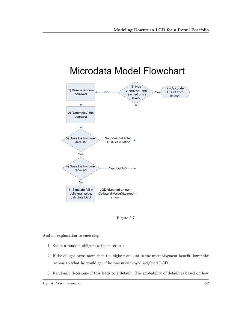
Modeling Downturn LGD for a Retail Portfolio
1) Draw a random
borrower
2) ”Unemploy” the
borrower
3) Does the borrower
default?
4) Does the borrower
recover?
5) Simulate fall in
collateral value,
calculate LGD
Yes
No
No, does not enter
DLGD calculation
Yes, LGD=0
6) Has
unemployment
reached crisis
level?
No Yes
7) Calculate
DLGD from
dataset
LGD=(Loaned amount-
Collateral Value)/Loaned
amount
Figure 5.7
And an explanation to each step
1. Select a random obligor (without return)
2. If the obligor earns more than the highest amount in the unemployment benefit, lower the
income to what he would get if he was unemployed.weighted LGD
3. Randomly determine if this leads to a default. The probability of default is based on how
By: A. Wirenhammar 52

Modeling Downturn LGD for a Retail Portfolio
much the income was lowered, on how high the interests rates are of the new income
a) If 3) does not leads to a default go to 6.
b) If 3) does leads to a default go to 4.
4. Calculated the risk for reemployment during the next year and randomly determine if this
obligor is reemployed,
5. If the obligor is reemployed LGD=0 and recovery=1 go to 6)
6. If 3) does not recover go to 5)
7. If he is not re-employed, simulate the fall in the value of the collateral by looking at
how much housing prices has fallen during historical recessions (or other indexes if the
collateral is not housing). If the new collateral value is still higher then the loaned amount
the LGD=0. Otherwise LGD=(Loaned amount-new collateral value)/ Loaned amount. Go
to 6.
8. Repeat the steps above until the ”unemployment” has been raised to a level that is similar
to the unemployment level in a historical crisis. So if the current unemployment is 4%
and the historical level of crisis unemployment is 10% we repeat these steps until we have
selected 10%-4%=6% of the loans portfolio and simulated them losing their jobs.
We then calculate the LGD we have in this scenario and use it as our downturn LGD.
This is of course a short overview on how this kind of model might work. If one were to use one
in real life one would have to define the distributions and refine the model.
By: A. Wirenhammar 53

Modeling Downturn LGD for a Retail Portfolio
By: A. Wirenhammar 54

Chapter 6
Results
6.1 Regression models
Using the regression model discussed above selecting which regression coefficients to use for each
pool by forward selection with a significance level of 0.05 we get the result in the tables below.
Please note that the intercepts are all numbers between 0 and 1. They have been left out for
confidentiality reasons since the intercept is very close to the average historical LGDs in our
dataset.
By: A. Wirenhammar 55

Modeling Downturn LGD for a Retail Portfolio
Country Pool Intercept GDP CPI Employment Unemployment Property Prices
Denmark Residential 0.xx
Denmark Unsecured 0.xx 0.28499 3.9392 -0.441 0.3159
Denmark Other 0.xx 9.3612
Finland Residential 0.xx 3.7915
Finland Unsecured 0.xx 1.16791 17.2707 -3.0182
Finland Other 0.xx
Norway Residential 0.xx 3.6544 -0.49612 1.4438
Norway Unsecured 0.xx -0.56812 -7.4129 -1.06481 2.1792
Norway Other 0.xx
Sweden Residential 0.xx
Sweden Unsecured 0.xx 0.19944
Sweden Other 0.xx 0.63988
Table 6.1
Country Pool Stock Index Yield 10Y Yield 5Y Yield 2Y Yield 3 months
Denmark Residential 0.33025
Denmark Unsecured 0.1148 -0.37061 0.27136
Denmark Other
Finland Residential 1.44616
Finland Unsecured 0.93215 0.02122 -0.48625
Finland Other 0.7527
Norway Residential 0.21316 -0.07645 -0.23496
Norway Unsecured 0.26361 -1.23574 1.0491 0.04746 -0.21879
Norway Other
Sweden Residential -0.21204
Sweden Unsecured -0.22528 -1.9865 1.06287
Sweden Other
Table 6.2
By: A. Wirenhammar 56

Modeling Downturn LGD for a Retail Portfolio
Regression DLGD
1 3 5 7 9 11 13 15 17 19 21 23 25 27 29 31 33 35 37
Pool nr
LG
D
Historical LGD 02-06
Predicted LGD 02-06
Predicted LGD 90-94
Figure 6.1
While regression models are a good idea in theory, they are not useful in practice to estimate
downturn LGD given the conditions in this paper. This is because, while the dataset used
contains hundred of thousand default observations, they are not representative for a downturn
period. This means that if we calculate the regression coefficients from these data, the coefficients
cannot be used to predict the LGD level in a downturn.
The results in table 6.1 and 6.2 is an aggregation of the full results some of the reasoning here
might not have support in these tables but are instead based on a larger table with a lot more
pools. The reason for censoring the results this way is commercial oonfidentiality.
The regression coefficients do show values that are clearly unreasonable. For example the coeffi-
cients for employment should all be negative, i.e. an increase in employment leads to a decrease
in LGD. This is however not the case, instead a number of pools for which employment is sig-
nificant, have a positive coefficient for employment. This means that if employment increases,
By: A. Wirenhammar 57

Modeling Downturn LGD for a Retail Portfolio
the LGD increases. This is clearly an unreasonable result and we can see the same pattern in
unemployment and property prices. We also have that increasing stock prices increases the LGD
for a number of pools.
If all the pools had the wrong sign it probably would depend on some other kind of error such
as omitted variable bias or multi-co-linearity. But when the signs are more or less randomly
distributed we have to draw the conclusion that regression is not usable with our dataset. In
the examples discussed above about 50 % of the pools has has a positive coefficient and 50%
has a negative coefficient. While the regression coefficients above obviously work reasonably well
to forecast the data that was used to calculate them, we cannot make any assumptions that
they can be used for anything else. This is based on what is reasonable with regards to how
the economy works and that all common sense speaks against such results. If the signs of the
regression coefficients were as expected, one might discuss using it to forecast a downturn but as
it is, that assumption cannot be made in good faith.
It is also important to note that the regression above is the specification that gives the best
results. All other specifications have given results that were worse, most of them a lot worse. For
example Appendix D contains the regression coefficients of all pools that are secured by private
housing on unemployment and property prices. As we can see, in the table, the sign and size
of the regression coefficient vary wildly, meaning that a small decrease in unemployment may
increase the LGD a lot in one pool and lower it in another. It is easy to achieve even worse result
by changing the specification even more.
While the variables debt ratio, interest rate ratio and savings ratio should be good predictors from
an economic common sense perspective, the results speak otherwise. If these variables are added
to the regression, we get degenerated results that are clearly unreasonable. This also strengthens
the reasoning above, i.e. our regression cannot be used to forecast downturn LGD.
A good example of this is that the LGD predicted in a crisis like the nineties crisis gives a
negative LGD in the area 2 to 6 for some pools. This is clearly unreasonable. You do loss
200%-600% more if a loan defaults in a crisis values of 1.05-1.15 might have been reasonable but
you do not spend 6 millions to get back 1 million from a non performing obligor. There are two
possible reasons for this, 1) these macro-economic variables are only available on a yearly basis
which is a problem since we do our regressions on a quarterly basis. 2) that the development
of these variables in the period 2002-2006 is not representative for a full economic cycle; instead
By: A. Wirenhammar 58

Modeling Downturn LGD for a Retail Portfolio
they only capture the behavior in a very good period. This might affect these variables more
since the number of observations is just a fourth of the number of observations of the other
macro-economic variables.
The same thing can be said about the variable forced sales in Demark, it shows a decreasing
trend during the period 2002-2006 while the LGD for residential mortgages, the pool forced sales
should affect the most, for non recovered loans varies wildly.
This volatility is caused by the lack of non recovered defaults; most quarters have less than
10 data points. This is because while residential mortgages are the largest pool measured by
exposure, there are hardly any data points that have led to actual losses in this pool. Instead
almost all observation that has led to actual losses is in the unsecured category, thus we have a
significant mismatch. This means that we do not get a representative relationship between the
variables and that the regression coefficients are extremely non robust.
For the reasons above, these variables have been left out of the regression model.
6.2 Linear Multifactor Model
While this model has some obvious disadvantages such as not being based on purely quantitative
analysis, it is also the model that shows the best results. This is of course dependant on the
fact that the lack of appropriate data disturbs the calibration of the other models, while this
model depends on an economic theory, the legal situation, and expert opinions for calibration.
This makes it possible to create a model that gives reasonable results that can be defended
with economic reasonability and expert evaluations. Any numeric results for this model are not
presented because of commercial confidentiality.
6.3 Latent Variable Single Factor Model
This model gives strange results, which may because of two reasons, not enough calibration
data/calibration data not representative or that the model does not work. Test with a larger
simulated dataset give more reasonable results. The result however is not good enough to actually
use. This because while the σ and q parameters are reasonable at least one of the µ’s are
unreasonable, example of this is either negative, larger than 1. The LGD is not bounded at one
By: A. Wirenhammar 59

Modeling Downturn LGD for a Retail Portfolio
as there are observations with an LGD above one, however getting a µ above ones implies that
in an average state of the economy the LGD is above 1. This is simply not the case. Neither
Frye’s original formulas nor the ones I arrived at, give any results that are usable.
While the are other latent variable models that could give better results, these were not tested
since the chance of them working when the Frye model does not, probably due to data inade-
quacies, should be very low.
By: A. Wirenhammar 60

Chapter 7
Conclusion
As we have seen in the results above, most methods to calculate downturn LGD do produce
results that are unreasonable in some way. The reason for this is obviously our lack of data and
the fact that the period we have data from was an economic boom. This makes the data hard
to use as a basis for a downturn scenario. To be able to produce some actually usable results,
we choose methods based on economic knowledge and patterns in our data. While this method
creates a model that feels more logical and consistent with common sense, it does not have the
same quantitative backing but instead partly relies on experts.
To get data of sufficient quality we would have to experience a crisis like the property crisis in
the nineties again. While the recent financial crisis was very severe in some senses, loan losses in
the nordic countries did not increase that much. The period can thus not be used as a downturn
period in our sense except for Denmark which had a more severe crisis.
While Nordea will get more data as the years go by, this also lessens the need for a downturn
LGD model. When sufficient data has been amassed one might simply use the realized LGD
value from an actual downturn scenario as downturn LGD. However there will always issue if
the past can be used to predict te future so the modelling downturn LGD will always be of some
interest.
The latent variable models might work if one have more data or use another specification. This
category of models however has a big disadvantage, namely that the latent variable is inherently
unobservable. This makes it impossible to determine how much you should stress the variable.
By: A. Wirenhammar 61

Modeling Downturn LGD for a Retail Portfolio
For example, if the latent variable is standard normal distributed as in Frye’s model, how do
one know which systematic risk factor value should be used to represent a crisis? There is no
way to determine that but to assume that a crisis is equivalent to some quantile of the normal
distribution. Such assumptions are impossible to justify since we have to base our model on facts
and historical crises.
The model that is the most promising is the model based on microdata. This allows for a much
more realistic modeling at the same time as it is both intuitive and mathematically simple. The
biggest obstacle for this model is the data required, but as time goes, this kind of data will be
collected and used. In fact, this kind of data already exists within every bank. This since no
bank will lend money to private persons without knowing what they earn, what the collateral
is worth and if the obligor has a bad credit record. The problem is that the processes and data
systems have not been adapted to save this data in a way that makes it feasible to use for this
kind of modeling. But, in the future I believe it will be available, which makes this kind of model
possible.
The hypothesis in this paper was that LGD≈DLGD. While we have not been able to support
this with quantitative data, most aspects seem to point in that direction. Examples of this are
the experience from the nineties crisis and that the pricefalls although severe was limited in the
sense that it mostly hit the homeowners equity since the loan to value ratio was below 1 in most
cases, seems to point in this direction.
By: A. Wirenhammar 62

Bibliography
[1] Basel Committee on Banking Supervision, (June 2004), International Convergence of Cap-
ital Measurement and Capital Standards A Revised Framework, Bank of international Set-
tlements, Usually referred to as the Basel II Accord
[2] Basel Committee on Banking Supervision (2005), Guidance on Paragraph 468 of the Frame-
work Document, Bank of International Settlements
[3] Basel Committee on Banking Supervision (2005b), Working Paper No. 14 Studies on the
Validation of Internal Rating Systems, Bank of International Settlements
[4] Basel Committee on Banking Supervision (2005c), An Explanatory Note on the Basel II
IRB Risk Weight Functions, Bank of International Settlements
[5] Vytautas Valvonis (2008), Estimating EAD for retail exposures for Basel II purposes p79-
109. Journal of Credit Risk, Spring 2008
[6] Sveriges Riksbank, (2006), Finansiell stabilitet 2006:1
[7] Sveriges Riksbank, (2009) Finansiell stabilitet 2009:2
[8] Finansinspektionen, (2007), Att mata kreditrisk - erfarenheter fran Basel 2
[9] Jon Frye, (2000), Depressing Recoveries, Emerging Issues Series Supervision and Regulation
Department Federal Reserve Bank of Chicago
[10] Stefano Caselli, Stefano Gatti and Francesca Querci,(2008), The Sensitivity of the Loss
Given Default Rate to Systematic Risk: New Empirical Evidence on Bank Loans, Journal
of Financial Services Research
By: A. Wirenhammar 63

Modeling Downturn LGD for a Retail Portfolio
[11] Radovan Chalupka, Juraj Kopecsni (2008), Modelling Bank Loan LGD of Corporate and
SME Segments: A Case Stud, Charles University Prague, Faculty of Social Sciences, vol.
59(4), pages 360-382
[12] Franks et al. (2004), A comparative analysis of the recovery process and recovery rates for
private companies in the UK, France and Germany, Standard & Poor’s Risk Solutions
[13] Nordea, (2009), Nordea Annual Report 2009
[14] Nordbanken, (1992), Nordbanken Annual Report 1992
[15] Nordbanken, (1993), Nordbanken Annual Report 1993
[16] Nordbanken, (1994), Nordbanken Annual Report 1994
[17] Dagens Industri, (31/8 2010), Ovantad uppgang for korta bolan
[18] Bruce E Hansen, (2010), Econometrics,University of Wisconsin
[19] Bogie Ozdemir and Peter Miu (2009), Basel II implementation: A guide to developing and
validating a compliant internal risk system, McGraw-Hill
[20] Bogie Ozdemir and Peter Miu (2005), Basel Requirement of Downturn LGD: Modeling and
Estimating PD and LGD Correlations, Journal of Credit Risk, Volume 2, Number 2, Summer
2006
[21] Hui Li (2010), Downturn LGD: A Spot Recovery Approach, MRPA
[22] Kronofogdemyndigheten (2008), Alla vill gora ratt for sig, Kronofogdemyndigheten Solu-
tions
[23] Barbro Wickman-Parak, (2009), Fastighetsmarkanden och den finansiella krisen, Sveriges
Riksbank.
[24] Tor Jacobson, Jesper Linde, Kasper Roszbach, (2008) Bankruptcy and the Business Cycle:
Are SMEs Less Sensitive to Systematic Risk? Conference on Small Business Finance World
Bank
[25] Tony Bellotti and Jonathan Crook, (2009), Loss Given Default models for UK retail credit
cards, Credit Research Centre University of Edinburgh Business School
[26] Brooks Brady, Peter Chang, Peter Miu, Bogie Ozdemir, David Schwartz (2006) Discount
Rate for Workout Recoveries: An empirical study, Working paper
By: A. Wirenhammar 64

Modeling Downturn LGD for a Retail Portfolio
[27] Yen-Ting Hu and William Perraudin (2002) The ependence of Recovery Rates and Defaults,
Working paper
[28] Dag Morten Dalen, Stephan L. Jervell, Eivind Smith, Anne Marie Nielsen, Anne Marie
Rø yert, Svein Harald Wiik, Lars Wohlin (1998) STORTINGETS GRANSKNINGSKOM-
MISJON FOR BANKKRISEN,
[29] Interview with Torbjorn Isaksson, Senior Analyst, 20/9 2010
[30] Interview with Troels Thiell Eriksen, Senior Analyst, 1/10 2010
[31] Interview with Stefan Blom, Credit Sweden at Nordea, 28/10 2010
[32] Interview with Kasper Roszbach, Deputy Head of research at Sveriges Riksbank, 11/10 2010
By: A. Wirenhammar 65

Modeling Downturn LGD for a Retail Portfolio
By: A. Wirenhammar 66

Appendix A
Table over macro data sources
The year the series starts in
By: A. Wirenhammar 67

Modeling Downturn LGD for a Retail Portfolio
Macro Variables Denmark Finland Norway Sweden
GDP 1990 1975 1978 1980
Consumer price index 1967 1960 1982 1900
Employment 1988 1988 1972 2001
Unemployment 1980 1959 1972 1991
Property prices 1992 1983 1989 1975
National Stock Index 1957 1957 1982 1987
Yield 10Y 1987 1991 1921 1918
Yield 5Y 1987 1948 1961 1986
Yield 2Y 1987 1992 1992 1960
Yield 3months 1972 1977 1971 1960
FX rate National Currency to EUR 1978 xxxx 1988 1978
LEAD 1968 1985 1970
Forced Sales 1984
Bankruptcies 1979 1986 1980 1994
Debt to disposable income ratio 1970*
Interest rate payments to disposable income ratio 1980*
Household financial savings 1988 1994*
Disposable income 1990 2002 1993*
This table show the year the macro data series start in, cells marked with * means that the data
only is available on a yearly basis instead of quarterly.
Collected from source
By: A. Wirenhammar 68

Modeling Downturn LGD for a Retail Portfolio
Macro Variables Denmark Finland Norway Sweden
GDP EW EW EW SCB
Consumer price index EW EW EW SCB
Employment EW EW EW EW
Unemployment EU EU EU+SSB EU
Property prices EW EW EW EW
National Stock Index EW EW EW EW
Yield 10Y EW EW EW EW
Yield 5Y EW EW EW EW
Yield 2Y EW EW EW EW
Yield 3months EW EW EW EW
FX rate National Currency to EUR EW EW EW
Forced Sales EW
Bankruptcies EW EW EW EW
Debt to disposable income ratio SCB
Interest rate payments to disposable income ratio SCB
Household financial savings EW SCB
Disposable income EW EW SCB
EW=EcoWin EUR=EuroStat SSB\SCB=National Statistics Agency.
By: A. Wirenhammar 69

Modeling Downturn LGD for a Retail Portfolio
By: A. Wirenhammar 70

Appendix B
Plots of macro data
Denmark GDP
0.00
50000.00
100000.00
150000.00
200000.00
250000.00
300000.00
350000.00
400000.00
Mar-85
Mar-86
Mar-87
Mar-88
Mar-89
Mar-90
Mar-91
Mar-92
Mar-93
Mar-94
Mar-95
Mar-96
Mar-97
Mar-98
Mar-99
Mar-00
Mar-01
Mar-02
Mar-03
Mar-04
Mar-05
Mar-06
Mar-07
Mar-08
Mar-09
Mar-10
GDP
Figure B.9
By: A. Wirenhammar 71
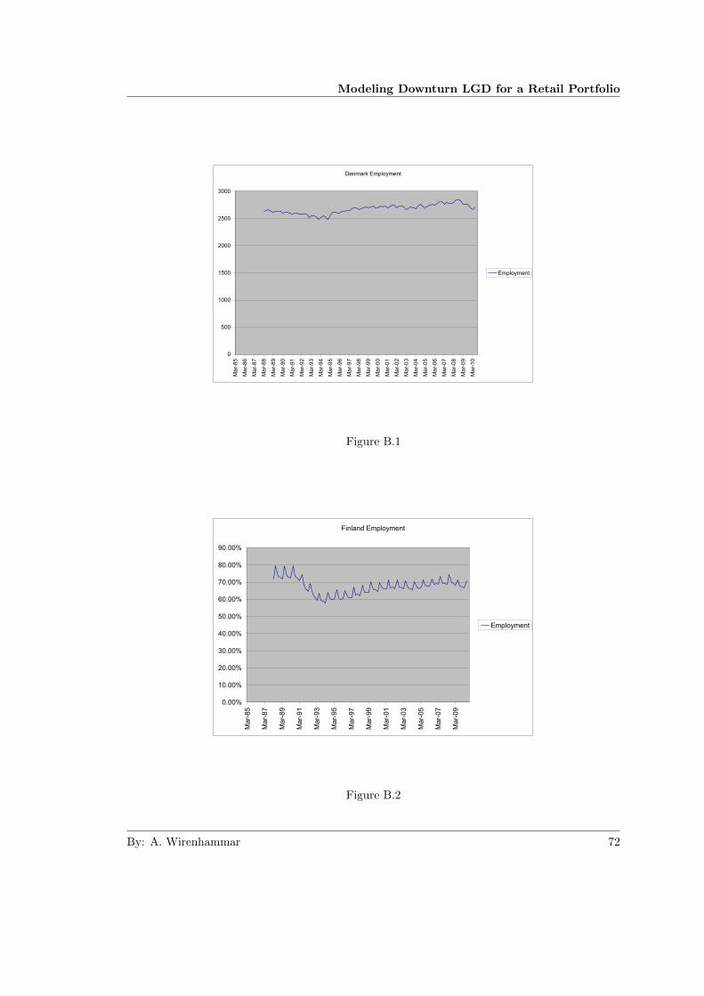
Modeling Downturn LGD for a Retail Portfolio
Denmark Employment
0
500
1000
1500
2000
2500
3000
Ma
r-8
5
Ma
r-8
6
Ma
r-8
7
Ma
r-8
8
Ma
r-8
9
Ma
r-9
0
Ma
r-9
1
Ma
r-9
2
Ma
r-9
3
Ma
r-9
4
Ma
r-9
5
Ma
r-9
6
Ma
r-9
7
Ma
r-9
8
Ma
r-9
9
Ma
r-0
0
Ma
r-0
1
Ma
r-0
2
Ma
r-0
3
Ma
r-0
4
Ma
r-0
5
Ma
r-0
6
Ma
r-0
7
Ma
r-0
8
Ma
r-0
9
Ma
r-1
0
Employment
Figure B.1
Finland Employment
0.00%
10.00%
20.00%
30.00%
40.00%
50.00%
60.00%
70.00%
80.00%
90.00%
Ma
r-8
5
Ma
r-8
7
Ma
r-8
9
Ma
r-9
1
Ma
r-9
3
Ma
r-9
5
Ma
r-9
7
Ma
r-9
9
Ma
r-0
1
Ma
r-0
3
Ma
r-0
5
Ma
r-0
7
Ma
r-0
9
Employment
Figure B.2
By: A. Wirenhammar 72

Modeling Downturn LGD for a Retail Portfolio
Norway Employment
0.00
500.00
1000.00
1500.00
2000.00
2500.00
3000.00
31/0
3/1
985
31/0
3/1
987
31/0
3/1
989
31/0
3/1
991
31/0
3/1
993
31/0
3/1
995
31/0
3/1
997
31/0
3/1
999
31/0
3/2
001
31/0
3/2
003
31/0
3/2
005
31/0
3/2
007
31/0
3/2
009
Employment
Figure B.3
Sweden Employment
0
500
1000
1500
2000
2500
3000
3500
4000
4500
5000
Ma
r-8
5
Ma
r-8
6
Ma
r-8
7
Ma
r-8
8
Ma
r-8
9
Ma
r-9
0
Ma
r-9
1
Ma
r-9
2
Ma
r-9
3
Ma
r-9
4
Ma
r-9
5
Ma
r-9
6
Ma
r-9
7
Ma
r-9
8
Ma
r-9
9
Ma
r-0
0
Ma
r-0
1
Ma
r-0
2
Ma
r-0
3
Ma
r-0
4
Ma
r-0
5
Ma
r-0
6
Ma
r-0
7
Ma
r-0
8
Ma
r-0
9
Ma
r-1
0
Employment
Figure B.4
By: A. Wirenhammar 73

Modeling Downturn LGD for a Retail Portfolio
Denmark Unemployment
0.00%
2.00%
4.00%
6.00%
8.00%
10.00%
12.00%
Mar
-85
Mar
-87
Mar
-89
Mar
-91
Mar
-93
Mar
-95
Mar
-97
Mar
-99
Mar
-01
Mar
-03
Mar
-05
Mar
-07
Mar
-09
Unemployment
Figure B.5
Finland Unemployment
0.00%
2.00%
4.00%
6.00%
8.00%
10.00%
12.00%
14.00%
16.00%
18.00%
20.00%
Mar
-85
Mar
-87
Mar
-89
Mar
-91
Mar
-93
Mar
-95
Mar
-97
Mar
-99
Mar
-01
Mar
-03
Mar
-05
Mar
-07
Mar
-09
Unemployment
Figure B.6
By: A. Wirenhammar 74

Modeling Downturn LGD for a Retail Portfolio
Norway Unemployment
0.0%
1.0%
2.0%
3.0%
4.0%
5.0%
6.0%
7.0%
8.0%M
ar-
85
Ma
r-8
7
Ma
r-8
9
Ma
r-9
1
Ma
r-9
3
Ma
r-9
5
Ma
r-9
7
Ma
r-9
9
Ma
r-0
1
Ma
r-0
3
Ma
r-0
5
Ma
r-0
7
Ma
r-0
9
Unemployment
Figure B.7
Sweden Unemployment
0.00%
2.00%
4.00%
6.00%
8.00%
10.00%
12.00%
Mar
-85
Mar
-87
Mar
-89
Mar
-91
Mar
-93
Mar
-95
Mar
-97
Mar
-99
Mar
-01
Mar
-03
Mar
-05
Mar
-07
Mar
-09
Unemployment
Figure B.8
By: A. Wirenhammar 75

Modeling Downturn LGD for a Retail Portfolio
Finland GDP
0.00
5000.00
10000.00
15000.00
20000.00
25000.00
30000.00
35000.00
40000.00
45000.00
50000.00
Ma
r-8
5
Ma
r-8
7
Ma
r-8
9
Ma
r-9
1
Ma
r-9
3
Ma
r-9
5
Ma
r-9
7
Ma
r-9
9
Ma
r-0
1
Ma
r-0
3
Ma
r-0
5
Ma
r-0
7
Ma
r-0
9
GDP
Figure B.10
Norway GDP
0
50000
100000
150000
200000
250000
300000
350000
400000
450000
31/0
3/1
985
31/0
3/1
986
31/0
3/1
987
31/0
3/1
988
31/0
3/1
989
31/0
3/1
990
31/0
3/1
991
31/0
3/1
992
31/0
3/1
993
31/0
3/1
994
31/0
3/1
995
31/0
3/1
996
31/0
3/1
997
31/0
3/1
998
31/0
3/1
999
31/0
3/2
000
31/0
3/2
001
31/0
3/2
002
31/0
3/2
003
31/0
3/2
004
31/0
3/2
005
31/0
3/2
006
31/0
3/2
007
31/0
3/2
008
31/0
3/2
009
31/0
3/2
010
GDP
Figure B.11
By: A. Wirenhammar 76

Modeling Downturn LGD for a Retail Portfolio
Sweden GDP
0.00
100000.00
200000.00
300000.00
400000.00
500000.00
600000.00
700000.00
800000.00
Mar-85
Mar-86
Mar-87
Mar-88
Mar-89
Mar-90
Mar-91
Mar-92
Mar-93
Mar-94
Mar-95
Mar-96
Mar-97
Mar-98
Mar-99
Mar-00
Mar-01
Mar-02
Mar-03
Mar-04
Mar-05
Mar-06
Mar-07
Mar-08
Mar-09
Mar-10
GDP
Figure B.12
Denmark Property Prices
0.00
20.00
40.00
60.00
80.00
100.00
120.00
Mar
-85
Mar
-87
Mar
-89
Mar
-91
Mar
-93
Mar
-95
Mar
-97
Mar
-99
Mar
-01
Mar
-03
Mar
-05
Mar
-07
Mar
-09
Property Prices
Figure B.13
By: A. Wirenhammar 77
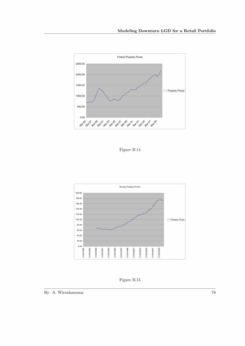
Modeling Downturn LGD for a Retail Portfolio
Finland Property Prices
0.00
500.00
1000.00
1500.00
2000.00
2500.00
Mar
-85
Mar
-87
Mar
-89
Mar
-91
Mar
-93
Mar
-95
Mar
-97
Mar
-99
Mar
-01
Mar
-03
Mar
-05
Mar
-07
Mar
-09
Property Prices
Figure B.14
Norway Property Prices
0.00
20.00
40.00
60.00
80.00
100.00
120.00
140.00
160.00
180.00
200.00
31/0
3/1
985
31/0
3/1
987
31/0
3/1
989
31/0
3/1
991
31/0
3/1
993
31/0
3/1
995
31/0
3/1
997
31/0
3/1
999
31/0
3/2
001
31/0
3/2
003
31/0
3/2
005
31/0
3/2
007
31/0
3/2
009
Property Prices
Figure B.15
By: A. Wirenhammar 78

Modeling Downturn LGD for a Retail Portfolio
Sweden Property Prices
0.00
100.00
200.00
300.00
400.00
500.00
600.00
Mar
-85
Mar
-87
Mar
-89
Mar
-91
Mar
-93
Mar
-95
Mar
-97
Mar
-99
Mar
-01
Mar
-03
Mar
-05
Mar
-07
Mar
-09
Property Prices
Figure B.16
Denmark Stock Index
0.00
100.00
200.00
300.00
400.00
500.00
600.00
Mar-85
Mar-87
Mar-89
Mar-91
Mar-93
Mar-95
Mar-97
Mar-99
Mar-01
Mar-03
Mar-05
Mar-07
Mar-09
Stock Index
Figure B.17
By: A. Wirenhammar 79

Modeling Downturn LGD for a Retail Portfolio
Finland Stock Index
0.00
2000.00
4000.00
6000.00
8000.00
10000.00
12000.00
14000.00
16000.00
18000.00
Ma
r-8
5
Ma
r-8
7
Ma
r-8
9
Ma
r-9
1
Ma
r-9
3
Ma
r-9
5
Ma
r-9
7
Ma
r-9
9
Ma
r-0
1
Ma
r-0
3
Ma
r-0
5
Ma
r-0
7
Ma
r-0
9
Stock Index
Figure B.18
Norway Stock Index
0.00
100.00
200.00
300.00
400.00
500.00
600.00
700.00
Mar
-85
Mar
-87
Mar
-89
Mar
-91
Mar
-93
Mar
-95
Mar
-97
Mar
-99
Mar
-01
Mar
-03
Mar
-05
Mar
-07
Mar
-09
Stock Index
Figure B.19
By: A. Wirenhammar 80

Modeling Downturn LGD for a Retail Portfolio
Sweden Stock Index
0.00
50.00
100.00
150.00
200.00
250.00
300.00
350.00
400.00
450.00
Mar-
85
Mar-
86
Mar-
87
Mar-
88
Mar-
89
Mar-
90
Mar-
91
Mar-
92
Mar-
93
Mar-
94
Mar-
95
Mar-
96
Mar-
97
Mar-
98
Mar-
99
Mar-
00
Mar-
01
Mar-
02
Mar-
03
Mar-
04
Mar-
05
Mar-
06
Mar-
07
Mar-
08
Mar-
09
Mar-
10
Stock Index
Figure B.20
Denmark Yield 2 Y
0.0%
2.0%
4.0%
6.0%
8.0%
10.0%
12.0%
14.0%
Mar-85
Mar-86
Mar-87
Mar-88
Mar-89
Mar-90
Mar-91
Mar-92
Mar-93
Mar-94
Mar-95
Mar-96
Mar-97
Mar-98
Mar-99
Mar-00
Mar-01
Mar-02
Mar-03
Mar-04
Mar-05
Mar-06
Mar-07
Mar-08
Mar-09
Mar-10
Yield 2 Y
Figure B.21
By: A. Wirenhammar 81

Modeling Downturn LGD for a Retail Portfolio
Finland Yield 2 Y
0.0%
2.0%
4.0%
6.0%
8.0%
10.0%
12.0%
14.0%
16.0%
Mar-85
Mar-86
Mar-87
Mar-88
Mar-89
Mar-90
Mar-91
Mar-92
Mar-93
Mar-94
Mar-95
Mar-96
Mar-97
Mar-98
Mar-99
Mar-00
Mar-01
Mar-02
Mar-03
Mar-04
Mar-05
Mar-06
Mar-07
Mar-08
Mar-09
Mar-10
Yield 2 Y
Figure B.22
Norway Yield 2 Y
0.00%
2.00%
4.00%
6.00%
8.00%
10.00%
12.00%
Ma
r-8
5
Ma
r-8
6
Ma
r-8
7
Ma
r-8
8
Ma
r-8
9
Ma
r-9
0
Ma
r-9
1
Ma
r-9
2
Ma
r-9
3
Ma
r-9
4
Ma
r-9
5
Ma
r-9
6
Ma
r-9
7
Ma
r-9
8
Ma
r-9
9
Ma
r-0
0
Ma
r-0
1
Ma
r-0
2
Ma
r-0
3
Ma
r-0
4
Ma
r-0
5
Ma
r-0
6
Ma
r-0
7
Ma
r-0
8
Ma
r-0
9
Ma
r-1
0
Yield 2 Y
Figure B.23
By: A. Wirenhammar 82

Modeling Downturn LGD for a Retail Portfolio
Sweden Yield 2 Y
0.00%
2.00%
4.00%
6.00%
8.00%
10.00%
12.00%
14.00%
16.00%
Mar-
85
Mar-
86
Mar-
87
Mar-
88
Mar-
89
Mar-
90
Mar-
91
Mar-
92
Mar-
93
Mar-
94
Mar-
95
Mar-
96
Mar-
97
Mar-
98
Mar-
99
Mar-
00
Mar-
01
Mar-
02
Mar-
03
Mar-
04
Mar-
05
Mar-
06
Mar-
07
Mar-
08
Mar-
09
Mar-
10
Yield 2 Y
Figure B.24
By: A. Wirenhammar 83

Modeling Downturn LGD for a Retail Portfolio
By: A. Wirenhammar 84

Appendix C
Pool Specification
Country Pool
Denmark Residential
Denmark Unsecured
Denmark Other
Finland Residential
Finland Unsecured
Finland Other
Norway Residential
Norway Unsecured
Norway Other
Sweden Residential
Sweden Unsecured
Sweden Other
By: A. Wirenhammar 85

Modeling Downturn LGD for a Retail Portfolio
By: A. Wirenhammar 86

Appendix D
Alternative Regressions
Country Pool Intercept Unemployment Property Prices
Denmark Residential 0.xx 0.66 5.72
Finland Residential 0.xx -2.60 3.13
Norway Residential 0.xx 0.05 0.15
Sweden Residential 0.xx 0.18 -1.72
By: A. Wirenhammar 87