Modeling Biological Systems in Stochastic

Concurrent Constraint Programming

Luca Bortolussi∗ Alberto Policriti†

Abstract

We present an application of stochastic Concurrent Constraint Programming(sCCP) for modeling biological systems. We provide a library of sCCP processesthat can be used to describe straightforwardly biological networks. In the mean-while, we show that sCCP proves to be a general and extensible framework,allowing to describe a wide class of dynamical behaviours and kinetic laws.

1 Introduction

Computational Systems Biology is an extremely fertile field, where many differentmodeling techniques are used [13, 7, 25, 37] in order to capture the intrinsic dynamicsof biological systems. These techniques are very different both in their spirit and inthe mathematics they use. Some of them are based on the well known instrumentof differential equations, mostly ordinary, and therefore they represent phenomena ascontinuous and deterministic, see [14] for a survey. On the other side we find stochasticand discrete models, that are usually simulated with Gillespie’s algorithm [21], tailoredfor simulating (exactly) chemical reactions. In the middle, we find hybrid approacheslike the chemical Langevin equation [17], a stochastic differential equation that partiallybridges these two opposite formalisms, and hybrid automata [1], mixing discrete andcontinuous evolution.

In the last few years a compositional modeling approach based on stochastic processalgebras (SPA) emerged [30], based on the inspiring parallel between molecules andreactions on one side and processes and communications on the other side [32]. Sto-chastic process algebras, like stochastic π-calculus [28], have a simple and powerfulsyntax and a stochastic semantics expressed in terms of Continuous Time MarkovChains [27], that can be simulated with an algorithm equivalent to Gillespie’s one.Since their introduction, SPA have been used to model, within the same framework,biological systems described at different level of abstractions, like biochemical reac-tions [29] and genetic regulatory networks [2].

Stochastic modeling of biological systems works by associating a rate to each activereaction (or, in general, interaction); rates are real numbers representing the frequencyor propensity of interactions. All active reactions then undergo a (stochastic) racecondition, and the fastest one is executed. Physical justification of this approach can

∗Dept. of Mathematics and Computer Science, University of Trieste, Italy. luca@dmi.units.it†Dept. of Mathematics and Computer Science, University of Udine, Italy.

policriti@dimi.uniud.it

1

be found in [20, 19]. These rates encode all the quantitative information in the system,and simulations produce discrete temporal traces with variable delay between events.

In this work we show how stochastic Concurrent Constraint Programming [3, 4](sCCP), another SPA recently developed, can be used for modeling biological sys-tems, extending the work presented in [5]. sCCP is based on Concurrent ConstraintProgramming [33] (CCP), a process algebra where agents interact by posting, at dif-ferent frequencies, constraints on the variables of the system in the constraint store,cf. Section 2.

In order to underline the rationale behind the usage of sCCP, we take an highlevel point of view, providing a general framework connecting elements of biologicalsystems with elements of the process algebra. Subsequently, we show how this generalframework gets instantiated when focused on particular classes of biological system,like networks of biochemical reactions and gene regulatory networks.

In our opinion, the advantages of using sCCP are twofold: the presence of bothquantitative information and computational capabilities at the level of the constraintsystems, and the presence of functional rates. This second feature, in particular, allowsto encode in the system different forms of dynamical behaviors, in a very flexible way.Quantitative information, on the other hand, allows a more compact representation ofmodels, as part of the details can be described in relations at the store’s level. Thecombined effect of these features not only allows the typical subdivision of the “logical”and “computational” part of the program, but also permits a non rigid introductionof the stochastic ingredient.

The paper is organized as follows: in Section 2 we review briefly sCCP, in Section 3we describe a high level mapping between biological systems and sCCP, then we in-stantiate the framework for biochemical reactions (Section 3.1) and gene regulatorynetworks (Section 3.2). Finally, in Section 4, we draw final conclusions and suggestfurther directions of investigation.

2 Stochastic Concurrent Constraint Programming

In this section we present a stochastic version [3] of Concurrent Constraint Program-ming [33], which will be used in the following as a modeling language for biologicalsystems. More material on sCCP ca be found in [4].

2.1 Concurrent Constraint Programming

Concurrent Constraint Programming (CCP [33]) is a process algebra having two dis-tinct entities: agents and constraints. Constraints are interpreted first-order logicalformulae, stating relationships among variables (e.g. X = 10 or X + Y < 7). CCP-agents compute by adding constraints (tell) into a “container” (the constraint store)and checking if certain relations are entailed by the current configuration of the con-straint store (ask). The communication mechanism among agents is therefore asyn-chronous, as information is exchanged through global variables. In addition to ask andtell, the language has all the basic constructs of process algebras: non-deterministicchoice, parallel composition, procedure call, plus the declaration of local variables.This dichotomy between agents and the constraint store can be seen as a form of sep-aration between computing capabilities (pertaining to the constraint store) and thelogic of interactions (pertaining to the agents). From a general point of view, the main

2

Program = D.A

D = ε | D.D | p(~x) : −A

A = 0 | tell∞(c) | M | ∃xA | A.A | A ‖ AM = π.G | M + M

π = tellλ(c) | askλ(c)G = 0 | tell∞(c) | p(~y) | M | ∃xG | G.G | G ‖ G

Table 1: Syntax of of sCCP.

difference between CCP and π-calculus resides really in the computational power ofthe former. π-calculus, in fact, has to describe everything in terms of communicationsonly, a fact that may result in cumbersome programs in all those situations in which“classical” computations are directly or indirectly involved.

The constraint store is defined as an algebraic lattice structure, using the theoryof cylindric algebras [22]. Essentially, we first choose a first-order language togetherwith an interpretation, which defines a semantical entailment relation (required tobe decidable). Then we fix a set of formulae, closed under finite conjunction, as theprimitive constraints that the agents can add to the store. The algebraic lattice isobtained by considering subsets of these primitive constraints, closed by entailmentand ordered by inclusion. The least upper bound operation of the lattice is denotedby t and it basically represents the conjunction of constraints. In order to model localvariables and parameter passing, the structure is enriched with cylindrification anddiagonalization operators, typical of cylindric algebras [22]. These operators allow todefine a sound notion of substitution of variables within constraints. In the followingwe denote the entailment relation by ` and a generic constraint store by C. We referto [12, 34, 33] for a detailed explanation of the constraint store management.

2.2 Syntax of sCCP

The stochastic version of CCP (sCCP [3, 4]) is obtained by adding a stochastic du-ration to the instructions interacting with the constraint store C, i.e. ask and tell.More precisely, each instruction is associated with a continuous random variable T ,representing the time needed to perform the corresponding operations in the store(i.e. adding or checking the entailment of a constraint). This random variable isexponentially distributed (cf. [27]), i.e. its probability density function is

f(τ) = λe−λτ , (2.1)

where λ is a positive real number, called the rate of the exponential random variable,which can be intuitively thought as the expected frequency per unit of time.

In our framework rates associated to ask and tell are functions

λ : C → R+,

3

an approach that allows us to link frequencies to the current configuration of theconstraint store. This means that the speed of communications can vary accordingto the particular state of the system, though in every state of the store the randomvariables are uniquely defined (their rate is evaluated to a real number). This fact givesto the language a remarkable flexibility in modeling biological systems, see Section 3for further material on this point.

The syntax of sCCP, as defined in [4], can be found in Table 1. An sCCP programconsists in a list of procedures declaration and in the starting configuration. Proce-dures are declared by specifying their name and their free variables, treated as formalparameters. Agents, on the other hand, are defined by the grammar in the last fourlines of Table 1. There are two different actions with temporal duration, i.e. ask andtell, identified by π. Their rate λ is a function as specified above. These actionscan be combined together into a guarded choice M (actually, a mixed choice, as weallow both ask and tell to be combined with summation). In this definition, we forceprocedure calls to be always guarded. In fact, they are instantaneous operations, thusguarding them by a timed action allows to avoid instantaneous infinite recursive loops,like those possible in p : −A ‖ p. In summary, an agent A can choose between differentactions (M), it can perform an instantaneous tell, it can declare a variable local(∃xA) or it can be combined in parallel with other agents.

A congruence relation among agents can be defined, ascribing the usual propertiesto the operators of the language (e.g. associativity and commutativity to + and ‖).The configurations of sCCP programs will vary in the quotient space modulo thiscongruence relation, denoted by P.

2.3 Operational Semantics of sCCP

The definition of the operational semantics is given specifying two different kinds oftransitions: one dealing with instantaneous actions and the other with stochasticallytimed ones. The basic idea of this operational semantics is to apply the two transi-tions in an interleaved way: first we apply the transitive closure of the instantaneoustransition, then we do one step of the timed stochastic transition. To identify a stateof the system, we need to take into account both the agents that are to be executedand the current configuration of the store. Therefore, a configuration will be a pointin the space P × C.

The recursive definition of the instantaneous transition −→⊆ (P × C)× (P × C) isshown in Table 2. Rule (IR1) models the addition of a constraint in the store throughthe least upper bound operation of the lattice. Recursion corresponds to rule (IR2),which consists in substituting the actual variables to the formal parameters in thedefinition of the procedure called. In rule (IR3), local variables are replaced by freshglobal variables, while in (IR4) the other rules are extended compositionally. Observethat we do not need to deal with summation operator at the level of instantaneoustransition, as all the choices are guarded by (stochastically) timed actions. The syn-tactic restrictions imposed to instantaneous actions guarantee that −→ can be appliedonly for a finite number of steps. Moreover, it can be proven to be confluent, see [4].Given a configuration 〈A, d〉 of the system, we denote by

−−−→〈A, d〉 the configuration ob-tained by applying the transitions −→ as long as it is possible (i.e., by applying thetransitive closure of −→). The confluence property of −→ implies that

−−−→〈A, d〉 is welldefined.

4

(IR1) 〈tell∞(c).A, d〉 −→ 〈A, d t c〉

(IR2) 〈p(x), d〉 −→ 〈A[x/y], d〉 if p(y) : −A

(IR3) 〈∃xA, d〉 −→ 〈A[y/x], d〉 with y fresh

(IR4)〈A1, d〉 −→ 〈A′1, d′〉

〈A1 ‖ A2, d〉 −→ 〈A′1 ‖ A2, d′〉

Table 2: Instantaneous transition for stochastic CCP

(SR1) 〈tellλ(c).A, d〉 =⇒(1,λ(d))−−−−−−→〈A, d t c〉

(SR2) 〈askλ(c).A, d〉 =⇒(1,λ(d))−−−→〈A, d〉 if d ` c

(SR3)〈M1, d〉 =⇒(p,λ)

−−−−→〈A′1, d′〉

〈M1 + M2, d〉 =⇒(p′,λ′)

−−−−→〈A′1, d′〉

with p′ = pλλ+rate(M2,d) and λ′ = λ + rate(M2, d)

(SR4)〈A1, d〉 =⇒(p,λ)

−−−−→〈A′1, d′〉

〈A1 ‖ A2, d〉 =⇒(p′,λ′)

−−−−−−−−−→〈A′1 ‖ A2, d

′〉with p′ = pλ

λ+rate(A2,d) and λ′ = λ + rate(A2, d)

Table 3: Stochastic transition relation for stochastic CCP

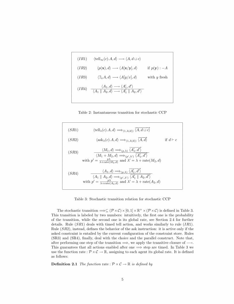
The stochastic transition =⇒⊆ (P×C)× [0, 1]×R+× (P×C) is defined in Table 3.This transition is labeled by two numbers: intuitively, the first one is the probabilityof the transition, while the second one is its global rate, see Section 2.4 for furtherdetails. Rule (SR1) deals with timed tell action, and works similarly to rule (IR1).Rule (SR2), instead, defines the behavior of the ask instruction: it is active only if theasked constraint is entailed by the current configuration of the constraint store. Rules(SR3) and (SR4), finally, deal with the choice and the parallel construct. Note that,after performing one step of the transition =⇒, we apply the transitive closure of −→.This guarantees that all actions enabled after one =⇒ step are timed. In Table 3 weuse the function rate : P ×C → R, assigning to each agent its global rate. It is definedas follows:

Definition 2.1 The function rate : P × C → R is defined by

5

1. rate (0, d) = 0;

2. rate (tellλ(c).A, d) = λ(d);

3. rate (askλ(c).A, d) = λ(d) if d ` c;

4. rate (askλ(c).A, d) = 0 if d 6` c;

5. rate (M1 + M2, d) = rate (M1, d) + rate (M2, d).

6. rate (A1 ‖ A2, d) = rate (A1, d) + rate (A2, d);

Using relation =⇒, we can build a labeled transition system, whose nodes areconfigurations of the system and whose labeled edges correspond to derivable stepsof =⇒. As a matter of fact, this is a multi-graph, as we can derive more than onetransition connecting two nodes (consider the case of tellλ(c)+tellλ(c)). Starting fromthis labeled graph, we can build a Continuous Time Markov Chain (cf. [27] and nextsection) as follows: substitute each label (p, λ) with the real number pλ and add up thenumbers labeling edges connecting the same nodes. More details about the operationalsemantics can be found in [3, 4].

2.4 Continuous Time Markov Chains and Gillespie’s Algorithm

A Continuous Time Markov Chain (CTMC for short) is a continuous-time stochasticprocess (Xt)t≥0 taking values in a discrete set of states S and satisfying the memorylessproperty, ∀n, t1, . . . , tn, s1, . . . , sn:

P{Xtn= sn | Xtn−1 = sn−1, . . . , Xt1 = s1} = P{Xtn

= sn | Xtn−1 = sn−1}. (2.2)

A CTMC can be represented as a directed graph whose nodes correspond to the statesof S and whose edges are labeled by real numbers, which are the rates of exponentiallydistributed random variables (defined by the probability density (2.1)). In each statethere are usually several exiting edges, competing in a race condition in such a waythat the fastest one is executed. The time employed by each transition is drawn fromthe random variable associated to it. When the system changes state, it forgets its pastactivity and starts a new race condition (this is the memoryless property). Therefore,the traces of a CTMC are made by a sequence of states interleaved by variable timedelays, needed to move from one state to another.

The time evolution of a CTMC can be characterized equivalently by computing,in each state, the normalized rates of the exit transitions and their sum (called theexit rate). The next state is then chosen according to the probability distributiondefined by the normalized rates, while the time spent for the transition is drawn froman exponentially distributed random variable with parameter equal to the exit rate.

This second characterization can be used in a Monte-Carlo simulation algorithm.Suppose to be in state s; then draw two random numbers, one according to the prob-ability given by the normalized rates, and the second according to an exponentialprobability distribution with parameter equal to the exit rate. Then choose the nextstate according to the first random number, and increase the time according to thesecond. The procedure sketched here is essentially the content of the Gillespie’s algo-rithm [20, 21], originally derived in the context of stochastic simulation of chemicalreactions. Indeed, the stochastic description of chemical reactions is exactly a Contin-uous Time Markov Chain [18].

6

2.5 Stream Variables

In the use of sCCP as a modeling language for biological systems, many variableswill represent quantities that vary over time, like the number of molecules of certainchemical species. In addition, the functions returning the stochastic rate of commu-nications will depend only on those variables. Unfortunately, the variables we haveat our disposal in CCP are rigid, in the sense that, whenever they are instantiated,they keep that value forever. However, time-varying variables can be easily modeled asgrowing lists with an unbounded tail: X = [a1, . . . , an|T ]. When the quantity changes,we simply need to add the new value, say b, at the end of the list by replacing the oldtail variable with a list containing b and a new tail variable: T = [b|T ′]. When we needto compute a function depending on the current value of the variable X, we need toextract from the list the value immediately preceding the unbounded tail. This can bedone by defining the appropriate predicates in the first-order language over which theconstraint store is built. As these variables have a special status in the presentationhereafter, we will refer to them as stream variables. In addition, we will use a simplifiednotation that hides all the details related to the list update. For instance, if we wantto add 1 to the current value of the stream variable X, we will simply write X = X+1.The intended meaning of this notation is clearly: “extract the last ground element nin the list X, consider its successor n + 1 and add it to the list (instantiating the oldtail variable as a list containing the new ground element and a new tail variable)”.

2.6 Implementation

We have developed an interpreter for the language that can be used for running sim-ulations. The simulation engine is based on the Gillespie’s Algorithm, therefore itperforms a Monte-Carlo simulation of the underlying CTMC. The memoryless prop-erty of the CTMC guarantees that we do need to generate all its nodes to perform asimulation, but we need to store only the current state. By syntactic analysis of thecurrent set of agents in execution, we can construct all the exit transitions and com-pute their rates, evaluating rate functions w.r.t. the current configuration of the store(actually, those functions depend only on stream variables, thus their computation hastwo steps: extract the current value of the variables and evaluate the function). Thenwe apply the Gillespie’s procedure to determine the next state and the elapsed time,updating the system by modifying the current set of agents and the constraint storeaccording to the chosen transition.

The interpreter is written in SICStus Prolog [16]. It is composed by a parser,accepting a program written in sCCP and converting it into an internal list-basedrepresentation. The main engine operates therefore by inspecting and manipulatingthe lists representing the program. The constraint store is managed using the con-straint solver on finite domains of SICStus. Stream variables are not represented aslists, but rather as global variables using the meta-predicates assert and retract ofProlog. The choice of working with finite domains is mainly related to the fact thatthe biological systems analyzed can be described using only integer values1.

In every execution cycle we need to inspect all terms in order to check if theyenable a transition. Therefore, the complexity of each step is linear in the size of the

1The real valued rates and the stochastic evolution are tight with the definition of the semanticsand not with the syntax of the language, thus we do not need to represent them in the store.

7

Measurable Entities ↔ Stream Variables

Logical Entities ↔ Processes(Control Variables)

Interactions ↔ Processes

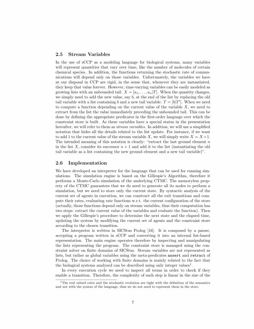
Table 4: Schema of the mapping between elements of biological systems (left) andsCCP (right).

(representation) of the program. This can be easily improved by observing that anenabled transition that is not executed remains enabled also in the future. See [4] forfurther details.

3 Modeling Biological Systems

Taking an high level point of view, biological systems can be seen as composed essen-tially by two ingredients: (biological) entities and interactions among those entities.For instance, in biochemical reaction networks, the molecules are the entities and thechemical reactions are the possible interactions, see [30] and Section 3.1. In gene reg-ulatory networks, instead, the entities into play are genes and regulatory proteins,while the interactions are production and degradation of proteins, and repression andenhancement of gene’s expression, cf. [2] and Section 3.2. In addition, entities fall intotwo separate classes: measurable and logical. Measurable entities are those presentin a certain quantity in the system, like proteins or other molecules. Logical entities,instead, have a control function (like gene gates in [2]), hence they are neither pro-duced nor degraded. Note that logical entities are not real world entities, but ratherthey are part of the models. Note that logical entities are not real world entities, butrather they are part of the models: genes, in fact, are concrete objects, made of atoms.However, they are present in one single copy, hence they are intrinsically different fromother molecules, fact that motivates their labeling as “logical”.

The translation scheme between the previously described elements and sCCP ob-jects is summarized in Table 4. Measurable entities are associated exactly to streamvariables introduced at the end of Section 2. Logical entities, instead, are representedas processes actively performing control activities. In addition, they can use variablesof the constraint store either as control variables or to exchange information. Finally,each interaction is associated to a process modifying the value of certain measurablestream variables of the system.

Associating variables to measurable entities means that we are representing themas part of the environment, while the active agents are associated to the differentactions capabilities of the system. These actions have a certain duration and a certainpropensity to happen: a fact represented here in the standard way, i.e. associatingto each action a stochastic rate. Actually, the speed of most of these actions dependson the quantity of the basic entities they act on. This fact shows clearly the need for

8

having functional rates, which can be used to describe these dependencies explicitly.This “interaction-centric” point of view, associating interactions to processes, is

different from the usual modeling activity of stochastic process algebras, like π-calculus,where each molecule is represented by a different process. The resulting approach,however, is still compositional, though what is composed together are interactionsrather than molecules. In the rest of the chapter, we show that this different approachdoes not result in models of bigger size (we are referring to the size of the syntacticdescription). Actually, the flexibility inherent in sCCP allows to take also an “entity-centric” point of view: we model genes as logical entities (gene gates), hence there canbe processes also associated to entities.

In the following, we instantiate this general scheme to deal with two classes of bio-logical systems: networks of biochemical reactions (Section 3.1) and genetic regulatorynetworks (Section 3.2). In both section, we provide some examples of systems describedand analyzed in sCCP. In particular, in Section 3.1.1, we show how to use functionalrates to write models where the complexity is reduced by using more complex rates(corresponding to more sophisticated chemical kinetics).

3.1 Modeling Biochemical Reactions

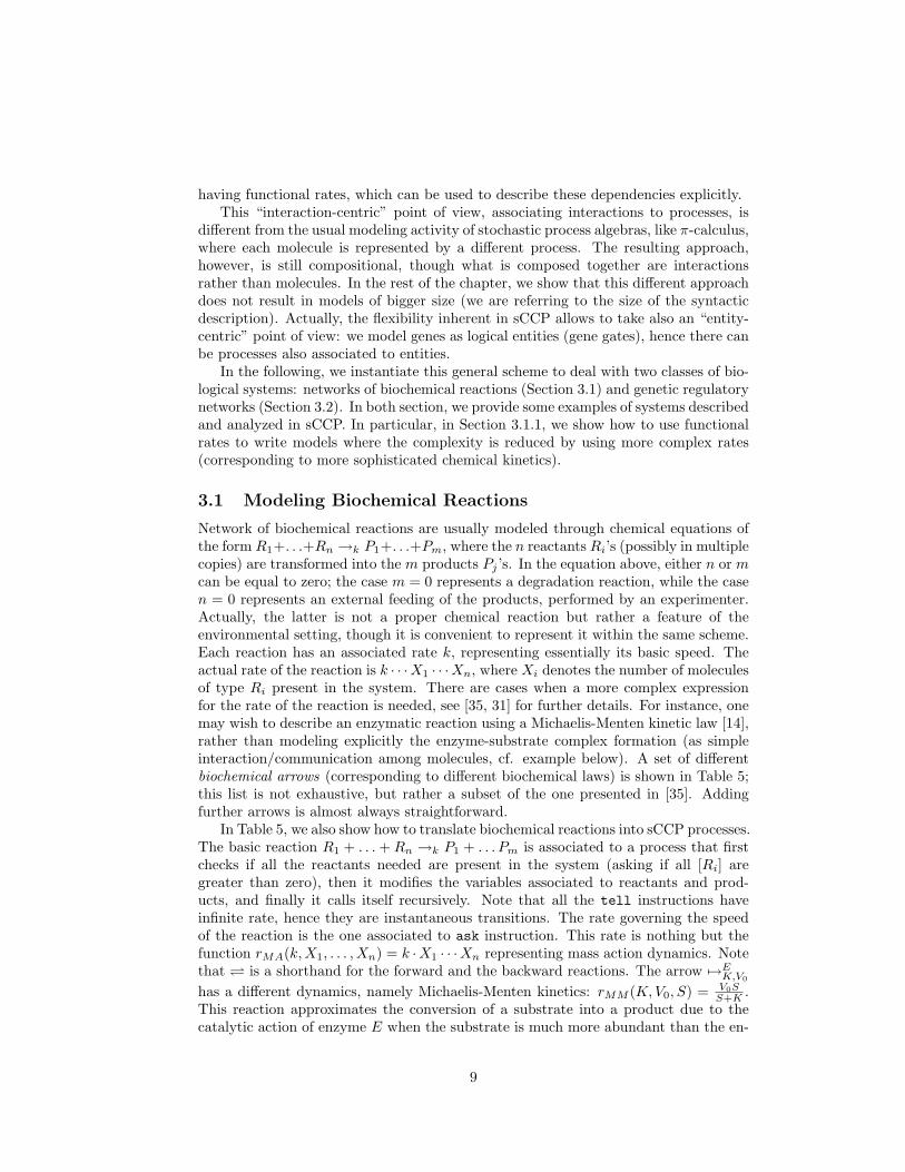
Network of biochemical reactions are usually modeled through chemical equations ofthe form R1+. . .+Rn →k P1+. . .+Pm, where the n reactants Ri’s (possibly in multiplecopies) are transformed into the m products Pj ’s. In the equation above, either n or mcan be equal to zero; the case m = 0 represents a degradation reaction, while the casen = 0 represents an external feeding of the products, performed by an experimenter.Actually, the latter is not a proper chemical reaction but rather a feature of theenvironmental setting, though it is convenient to represent it within the same scheme.Each reaction has an associated rate k, representing essentially its basic speed. Theactual rate of the reaction is k · · ·X1 · · ·Xn, where Xi denotes the number of moleculesof type Ri present in the system. There are cases when a more complex expressionfor the rate of the reaction is needed, see [35, 31] for further details. For instance, onemay wish to describe an enzymatic reaction using a Michaelis-Menten kinetic law [14],rather than modeling explicitly the enzyme-substrate complex formation (as simpleinteraction/communication among molecules, cf. example below). A set of differentbiochemical arrows (corresponding to different biochemical laws) is shown in Table 5;this list is not exhaustive, but rather a subset of the one presented in [35]. Addingfurther arrows is almost always straightforward.

In Table 5, we also show how to translate biochemical reactions into sCCP processes.The basic reaction R1 + . . . + Rn →k P1 + . . . Pm is associated to a process that firstchecks if all the reactants needed are present in the system (asking if all [Ri] aregreater than zero), then it modifies the variables associated to reactants and prod-ucts, and finally it calls itself recursively. Note that all the tell instructions haveinfinite rate, hence they are instantaneous transitions. The rate governing the speedof the reaction is the one associated to ask instruction. This rate is nothing but thefunction rMA(k,X1, . . . , Xn) = k ·X1 · · ·Xn representing mass action dynamics. Notethat is a shorthand for the forward and the backward reactions. The arrow 7→E

K,V0

has a different dynamics, namely Michaelis-Menten kinetics: rMM (K, V0, S) = V0SS+K .

This reaction approximates the conversion of a substrate into a product due to thecatalytic action of enzyme E when the substrate is much more abundant than the en-

9

R1 + . . . + Rn →k P1 + . . . + Pm

reaction(k, [R1, . . . , Rn], [P1, . . . , Pm]) : −askrMA(k,R1,...,Rn)

�Vni=1(Ri > 0)

�.�

‖ni=i tell∞(Ri = Ri − 1) ‖

‖mj=1 tell∞(Pj = Pj + 1)

�.

reaction(k, [R1, . . . , Rn], [P1, . . . , Pm])

R1 + . . . + Rn k1k2

P1 + . . . + Pmreaction(k1, [R1, . . . , Rn], [P1, . . . , Pm]) ‖reaction(k2, [P1, . . . , Pm], [R1, . . . , Rn])

S 7→EK,V0

P

mm reaction(K, V0, S, P ) : −askrMM (K,V0,S)(S > 0).(tell∞(S = S − 1) ‖ tell∞(P = P + 1)) .mm reaction(K, V0, S, P )

S 7→EK,V0,h P

hill reaction(K, V0, h, S, P ) : −askrHill(K,V0,h,S)(S > 0).(tell∞(S = S − h) ‖ tell∞(P = P + h)) .Hill reaction(K, V0, h, S, P )

whererMA(k, X1, . . . , Xn) = k ·X1 · · ·Xn

rMM (K, V0, S) = V0SS+K

rHill(k, V0, h, S) = V0Sh

Sh+Kh

Table 5: Translation into sCCP of different biochemical reaction types, taken from thelist of [35]. The reaction process models a mass-action-like reaction. It takes in inputthe basic rate of the reaction, the list of reactants, and the list of products. Theselist can be empty, corresponding to degradation and external feeding. The processhas a blocking guard that checks if all the reactants are present in the system. Therate of the ask is exactly the global rate of the reaction. If the process overcomesthe guard, it modifies the quantity of reactants and products and then it calls itselfrecursively. The reversible reaction is modeled as the combination of binding andunbinding. The third arrow corresponds to a reaction with Michaelis-Menten kinetics.The corresponding process works similarly to the first reaction, but the rate functionis different. Here, in fact, the rate function is the one expressing Michaelis-Mentenkinetics. See Section 3.1.1 for further details. The last arrow replaces Michaelis-Mentenkinetics with Hill’s one (see end of Section 3.1.1).

zyme (quasi-steady state assumption, cf. [14]). The last arrow, instead, is associatedto Hill’s kinetics. The dynamics represented here is an improvement on the Michaelis-Menten law, where the exponent h encodes some information about the cooperativityof enzymatic binding.

Comparing the encoding of biochemical reaction into sCCP with the encoding intoother process algebras like π-calculus [30], we note that the presence of functionalrates gives more flexibility in the modeling phase. In fact, these rates allow to describedynamics that are different from Mass Action. Notable examples are exactly Michaelis-Menten’s and Hill’s cases, represented by the last two arrows. This is not possiblewherever only constant rates are present, as the definition of the operational semantics

10

enz reaction(k1, k−1, k2, S, E,ES, P ) :-reaction(k1, [S, E], [ES]) ‖ reaction(k−1, [ES], [E,S]) ‖ reaction(k2, [ES], [E,P ]).

enz reaction(k1, k−1, k2, S, E,ES, P ) ‖ reaction(kprod, [], [S]) ‖ reaction(kdeg, [P ], [])

Table 6: sCCP program for an enzymatic reaction with mass action kinetics. Thefirst block defines the predicate enz reaction(k1, k−1, k2, S, E,ES, P ), while the secondblock is the definition of the entire program. The predicate reaction has been definedin Table 5.

constrain the dynamics to be Mass-Action like. More comments about this fact canbe found in [6, 4].

3.1.1 Example: Enzymatic Reaction

As a first and simple example, we show the model of an enzymatic reaction. Weprovide two different descriptions, one using a mass action kinetics, the other using aMichaelis-Menten one, see Table 5.

In the first case, we have the following set of reactions:

S + E k1k−1

ES →k2 P + E; P →kdeg; →kprod

S, (3.1)

corresponding to a description of an enzymatic reaction that takes into account alsothe enzyme-substrate complex formation. Specifically, substrate S and enzyme Ecan bind and form the complex ES. This complex can either dissociate back into Eand S, or be converted into the product P and again enzyme E. Moreover, in thisparticular system we added degradation of P and external feeding of S, in order to havecontinuous production of P . The sCCP model of this reaction can be found in Table 6.It is simply composed by 5 reaction agents, one for each arrow of the equations (3.1).The three reactions involving the enzyme are grouped together under the predicateenz_reaction{k1,k-1,k2,S,E,ES,P}, that will be used in following subsections.

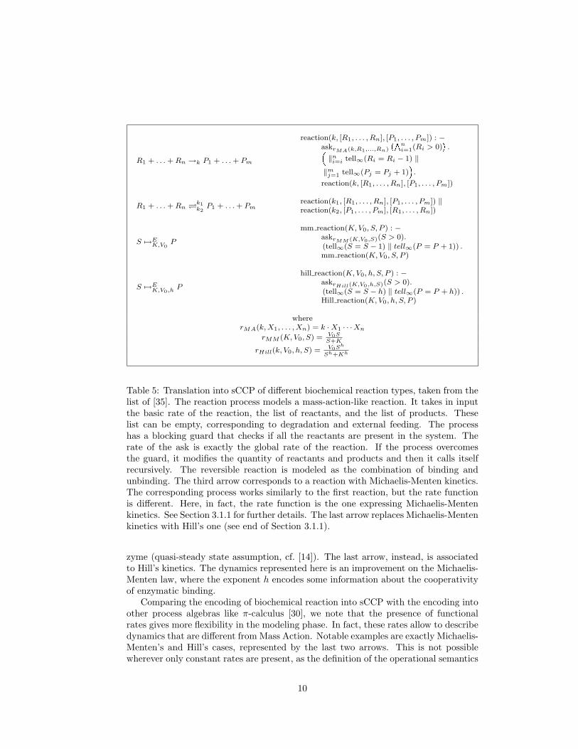
Simulations were performed with the simulator described in Section 2.6, and thetrend of product P is plotted in Figure 1 (top). Parameters of the system were chosenin order to have, at regime, almost all the enzyme molecules in the complexed state,see caption of Figure 1 (top) for details.

For this simple enzymatic reaction, the quasi-steady state assumption [14] can beapplied, thanks to the fact that the number of molecules of the substrate is much biggerthan the number of molecules of the enzyme (meaning that almost all molecules ofthe enzyme are in the complexed form). Therefore, replacing the substrate-enzymecomplex formation with a Michaelis-Menten kinetics (see [14]) should leave the systembehaviour unaltered. This intuition is confirmed by Figure 1 (bottom), showing theplot of the evolution over time of product P for the following system of reactions:

S 7→EK,V0

P ; P →kdeg; →kprod

S,

whose sCCP code can be derived easily from Table 5.Actually, the two graphs in Figure 1 are similar is not just by chance, but rather as a

consequence of a general result of Rao [31] about the use of steady state assumption instochastic simulation. This can be seen as an approximate technique for model simpli-fication, that reduces the dimension of the state space by averaging out the behaviour

11

Figure 1: (top) Mass Action dynamics for an enzymatic reaction. The graph showsthe time evolution of the product P . Rates used in the simulation are k1 = 0.1,k−1 = 0.001, k2 = 0.5, kdeg = 0.01, kprod = 5. Enzyme molecules E are never degraded(though they can be in the complex status), and initial value is set to E = 10. Startingvalue for S is 100, while for P is zero. Notice that the rate of complexation of E andS into ES and the dissociation rate of ES into E and P are much bigger than thedissociation rate of ES into E and S. This implies that almost all the moleculesof E will be found in the complexed form. (bottom) Michaelis-Menten dynamicsfor an enzymatic reaction. The graph shows the time evolution of the product P .Rates kdeg and kprod are the same as above, whilst K = 5.01 and V0 = 5. These lastvalues are derived from mass action rates in the standard way, i.e. K = K2+k−1

k1and

V0 = k2E0, where E0 is the starting quantity of enzyme E, cf. [14] for a derivationof these expressions. Notice that the time spawn by this second temporal series islonger than the first one, despite the fact that simulations lasted the same numberof elementary steps (of the labeled transition system of sCCP). This is because theproduct formation in the Michaelis-Menten dynamics model is a one step reaction,while in the other system it is a two step reaction (with a possible loop because of thedissociation of ES into E and S).

of some variables of the system. This averaging procedure induces a complication ofthe form of the stochastic rates of the models. In the case of Michaelis-Menten dy-

12

namics, it can be shown [31] that the stochastic and the deterministic form for therates under quasi-steady state assumption coincide; this gives a formal justification forthe adoption of the simplified model shown above. In [31], the authors claim also thatthis correspondence in the form of rates should hold also for other, more complicated,approximations induced by quasi-steady state assumption, like that of Hill’s equations.

Hill’s equation treat the case in which some level of cooperativity of the enzyme isto be modeled (see [10]). The set of reactions in this case is an extension of the aboveone and, for a cooperative effect of degree two, can be written as:

S + E k1k−1

C1 →k2 P + E;S + C1 k3

k−3C2 →k4 P + E;

P →kdeg; →kprod

S.

(3.2)

The corresponding sCCP program is a straightforward extension of the previousone:

2 enz reaction(k1, k−1, k2, k3, k−3, k4, S, E,ES, P ) :-reaction(k1, [S, E], [C1]) ‖ reaction(k−1, [C1], [E,S]) ‖ reaction(k2, [C1], [E,P ]) ‖reaction(k3, [S, C1], [C2]) ‖ reaction(k−3, [C2], [C1, S]) ‖ reaction(k4, [C2], [E,P ])

while the rest of the coding is entirely similar to the previous case.Also in this case a comparison with the reaction obtained with the computed Hill

coefficientS 7→E

K,V0,2 P ; P →kdeg; →kprod

S,

can be easily carried out. This kinetics, however, can be used only under some as-sumptions on the value of the rates involved, see [4] for further details. Notice thatthe Hill’s exponent corresponds exactly to the degree of cooperativity of the enzyme,2 in this case. Generalization to enzymatic reaction of higher order cooperativity isstraightforward. In Figure 2, we compare two simulations, one carried out with thefull model and one carried out with the reduced model, using the corresponding Hillkinetics. As we can see, the two trajectories are almost coincident.

3.1.2 Example: MAP-Kinase Cascade

A cell is not an isolated system, but it communicates with the external environmentusing complex mechanisms. In particular, a cell is able to react to external signals, i.e.to signaling proteins (like hormones) present in the proximity of the external mem-brane. Roughly speaking, this membrane is filled with receptor proteins, that have apart exposed toward the external environment capable of binding with the signalingprotein. This binding modifies the structure of the receptor protein, that can now trig-ger a chain of reactions inside the cell, transmitting the signal straight to the nucleus.In this signaling cascade a predominant part is performed by a family of proteins,called Kinase, that have the capability of phosphorylating other proteins. Phospho-rylation is a modification of the protein fold by attaching a phosphorus molecule toa particular amino acid of the protein. One interesting feature of these cascades ofreactions is that they are activated only if the external stimulus is strong enough. Inaddition, the activation of the protein at the end of the chain of reactions (usually an

13

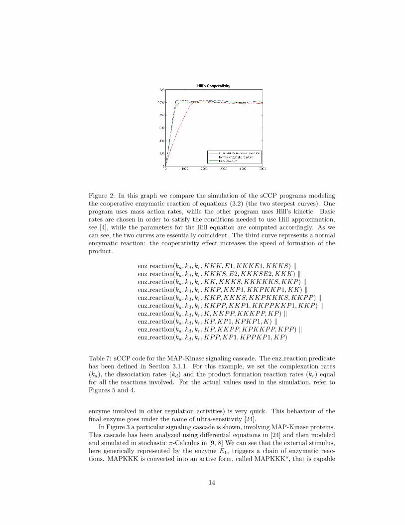
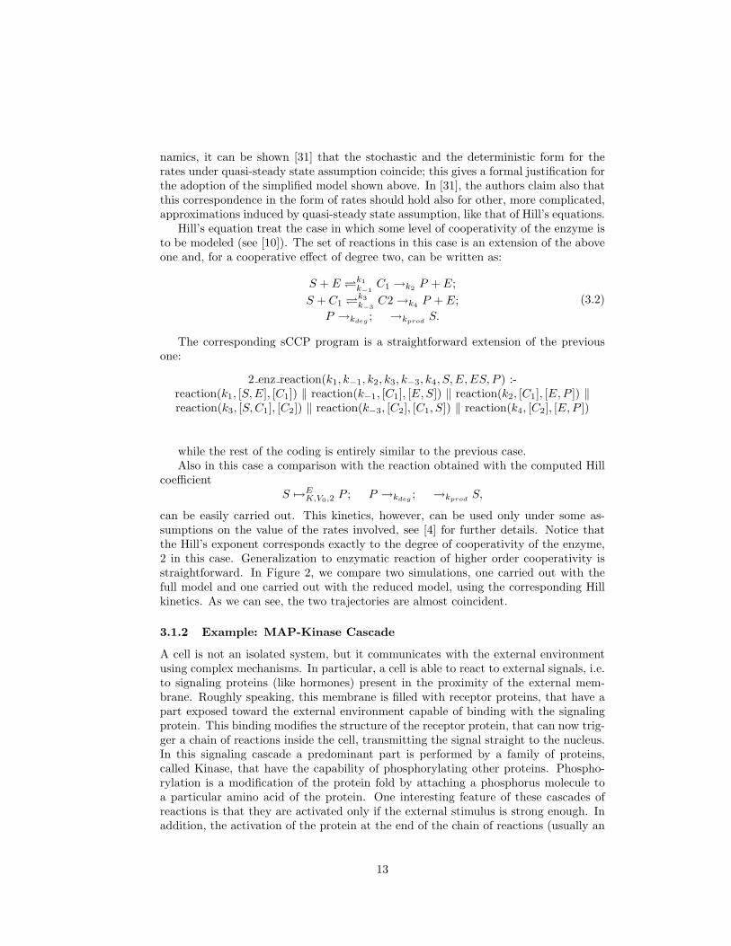
Figure 2: In this graph we compare the simulation of the sCCP programs modelingthe cooperative enzymatic reaction of equations (3.2) (the two steepest curves). Oneprogram uses mass action rates, while the other program uses Hill’s kinetic. Basicrates are chosen in order to satisfy the conditions needed to use Hill approximation,see [4], while the parameters for the Hill equation are computed accordingly. As wecan see, the two curves are essentially coincident. The third curve represents a normalenzymatic reaction: the cooperativity effect increases the speed of formation of theproduct.

enz reaction(ka, kd, kr,KKK, E1,KKKE1,KKKS) ‖enz reaction(ka, kd, kr,KKKS,E2,KKKSE2,KKK) ‖enz reaction(ka, kd, kr,KK, KKKS,KKKKKS, KKP ) ‖enz reaction(ka, kd, kr,KKP,KKP1,KKPKKP1,KK) ‖enz reaction(ka, kd, kr,KKP,KKKS,KKPKKKS, KKPP ) ‖enz reaction(ka, kd, kr,KKPP,KKP1,KKPPKKP1,KKP ) ‖enz reaction(ka, kd, kr,K,KKPP, KKKPP,KP ) ‖enz reaction(ka, kd, kr,KP,KP1,KPKP1,K) ‖enz reaction(ka, kd, kr,KP,KKPP,KPKKPP,KPP ) ‖enz reaction(ka, kd, kr,KPP,KP1,KPPKP1,KP )

Table 7: sCCP code for the MAP-Kinase signaling cascade. The enz reaction predicatehas been defined in Section 3.1.1. For this example, we set the complexation rates(ka), the dissociation rates (kd) and the product formation reaction rates (kr) equalfor all the reactions involved. For the actual values used in the simulation, refer toFigures 5 and 4.

enzyme involved in other regulation activities) is very quick. This behaviour of thefinal enzyme goes under the name of ultra-sensitivity [24].

In Figure 3 a particular signaling cascade is shown, involving MAP-Kinase proteins.This cascade has been analyzed using differential equations in [24] and then modeledand simulated in stochastic π-Calculus in [9, 8] We can see that the external stimulus,here generically represented by the enzyme E1, triggers a chain of enzymatic reac-tions. MAPKKK is converted into an active form, called MAPKKK*, that is capable

14

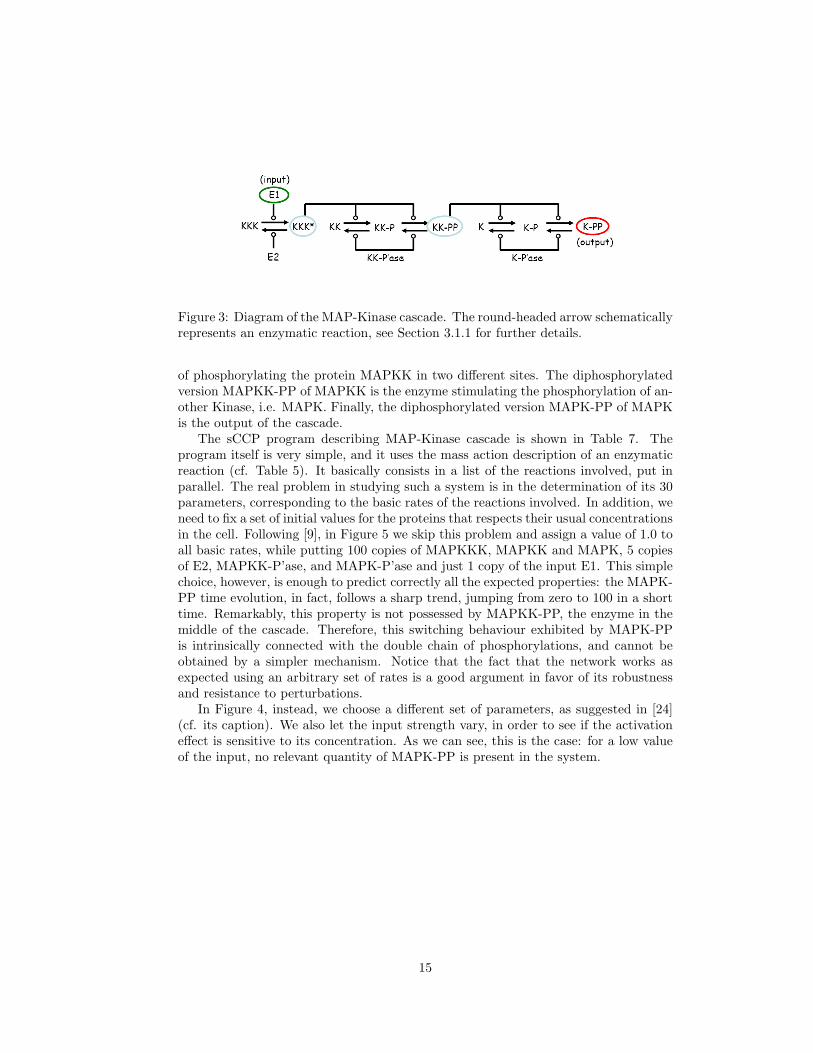
Figure 3: Diagram of the MAP-Kinase cascade. The round-headed arrow schematicallyrepresents an enzymatic reaction, see Section 3.1.1 for further details.

of phosphorylating the protein MAPKK in two different sites. The diphosphorylatedversion MAPKK-PP of MAPKK is the enzyme stimulating the phosphorylation of an-other Kinase, i.e. MAPK. Finally, the diphosphorylated version MAPK-PP of MAPKis the output of the cascade.

The sCCP program describing MAP-Kinase cascade is shown in Table 7. Theprogram itself is very simple, and it uses the mass action description of an enzymaticreaction (cf. Table 5). It basically consists in a list of the reactions involved, put inparallel. The real problem in studying such a system is in the determination of its 30parameters, corresponding to the basic rates of the reactions involved. In addition, weneed to fix a set of initial values for the proteins that respects their usual concentrationsin the cell. Following [9], in Figure 5 we skip this problem and assign a value of 1.0 toall basic rates, while putting 100 copies of MAPKKK, MAPKK and MAPK, 5 copiesof E2, MAPKK-P’ase, and MAPK-P’ase and just 1 copy of the input E1. This simplechoice, however, is enough to predict correctly all the expected properties: the MAPK-PP time evolution, in fact, follows a sharp trend, jumping from zero to 100 in a shorttime. Remarkably, this property is not possessed by MAPKK-PP, the enzyme in themiddle of the cascade. Therefore, this switching behaviour exhibited by MAPK-PPis intrinsically connected with the double chain of phosphorylations, and cannot beobtained by a simpler mechanism. Notice that the fact that the network works asexpected using an arbitrary set of rates is a good argument in favor of its robustnessand resistance to perturbations.

In Figure 4, instead, we choose a different set of parameters, as suggested in [24](cf. its caption). We also let the input strength vary, in order to see if the activationeffect is sensitive to its concentration. As we can see, this is the case: for a low valueof the input, no relevant quantity of MAPK-PP is present in the system.

15

Figure 4: Comparison of the temporal evolution of the MAP-Kinase cascade for dif-ferent concentrations of the enzyme MAPKKK. As argued in [24], this is equivalentto the variation of the input signal E1. Rates are equal for all reactions, and have thefollowing values: ka = 1, kd = 150, kr = 150. This corresponds to a Michaelis-Mentenrate of 300 for all the enzymatic reactions. The initial quantity of MAPKK and MAPKis set to 1200, the initial quantity of phosphatase MAPK-P’ase is set to 120, the initialquantity of other phosphatase and the enzyme E2 is set to 5, and the initial quantityof E1 is 1. (top) The initial quantity of MAPKKK is 3. We can see that there is nosensible production of MAPK-PP. (middle) The initial quantity of MAPKKK is 30.Enzyme MAPK-PP is produced but its trend is not sharp, as expected. (bottom)The initial quantity of MAPKKK is 300. The system behaves as expected. We can seethat the increase in the concentration of MAPK-PP is very sharp, while MAPKK-PPgrows very slowly in comparison.

16

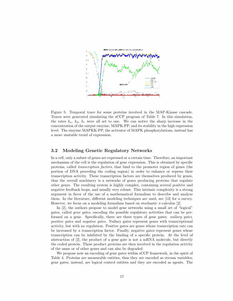
Figure 5: Temporal trace for some proteins involved in the MAP-Kinase cascade.Traces were generated simulating the sCCP program of Table 7. In this simulation,the rates ka, kd, kr were all set to one. We can notice the sharp increase in theconcentration of the output enzyme, MAPK-PP, and its stability in the high expressionlevel. The enzyme MAPKK-PP, the activator of MAPK phosphorylations, instead hasa more unstable trend of expression.

3.2 Modeling Genetic Regulatory Networks

In a cell, only a subset of genes are expressed at a certain time. Therefore, an importantmechanism of the cell is the regulation of gene expression. This is obtained by specificproteins, called transcription factors, that bind to the promoter region of genes (theportion of DNA preceding the coding region) in order to enhance or repress theirtranscription activity. These transcription factors are themselves produced by genes,thus the overall machinery is a networks of genes producing proteins that regulateother genes. The resulting system is highly complex, containing several positive andnegative feedback loops, and usually very robust. This intrinsic complexity is a strongargument in favor of the use of a mathematical formalism to describe and analyzethem. In the literature, different modeling techniques are used, see [13] for a survey.However, we focus on a modeling formalism based on stochastic π-calculus [2].

In [2], the authors propose to model gene networks using a small set of “logical”gates, called gene gates, encoding the possible regulatory activities that can be per-formed on a gene. Specifically, there are three types of gene gates: nullary gates,positive gates and negative gates. Nullary gates represent genes with transcriptionalactivity, but with no regulation. Positive gates are genes whose transcription rate canbe increased by a transcription factor. Finally, negative gates represent genes whosetranscription can be inhibited by the binding of a specific protein. At the level ofabstraction of [2], the product of a gene gate is not a mRNA molecule, but directlythe coded protein. These product proteins are then involved in the regulation activityof the same or of other genes and can also be degraded.

We propose now an encoding of gene gates within sCCP framework, in the spirit ofTable 4. Proteins are measurable entities, thus they are encoded as stream variables;gene gates, instead, are logical control entities and they are encoded as agents. The

17

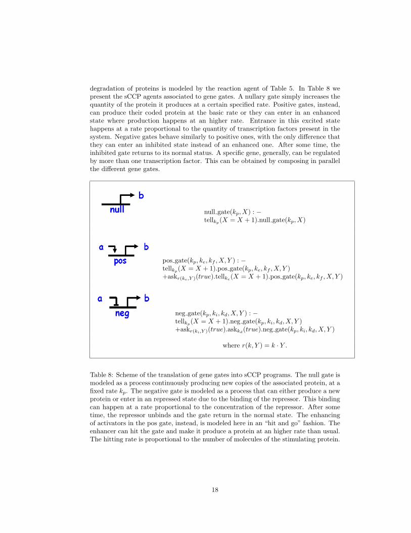
degradation of proteins is modeled by the reaction agent of Table 5. In Table 8 wepresent the sCCP agents associated to gene gates. A nullary gate simply increases thequantity of the protein it produces at a certain specified rate. Positive gates, instead,can produce their coded protein at the basic rate or they can enter in an enhancedstate where production happens at an higher rate. Entrance in this excited statehappens at a rate proportional to the quantity of transcription factors present in thesystem. Negative gates behave similarly to positive ones, with the only difference thatthey can enter an inhibited state instead of an enhanced one. After some time, theinhibited gate returns to its normal status. A specific gene, generally, can be regulatedby more than one transcription factor. This can be obtained by composing in parallelthe different gene gates.

null gate(kp, X) : −tellkp

(X = X + 1).null gate(kp, X)

pos gate(kp, ke, kf , X, Y ) : −tellkp

(X = X + 1).pos gate(kp, ke, kf , X, Y )+askr(ke,Y )(true).tellke

(X = X + 1).pos gate(kp, ke, kf , X, Y )

neg gate(kp, ki, kd, X, Y ) : −tellkp

(X = X + 1).neg gate(kp, ki, kd, X, Y )+askr(ki,Y )(true).askkd

(true).neg gate(kp, ki, kd, X, Y )

where r(k, Y ) = k · Y .

Table 8: Scheme of the translation of gene gates into sCCP programs. The null gate ismodeled as a process continuously producing new copies of the associated protein, at afixed rate kp. The negative gate is modeled as a process that can either produce a newprotein or enter in an repressed state due to the binding of the repressor. This bindingcan happen at a rate proportional to the concentration of the repressor. After sometime, the repressor unbinds and the gate return in the normal state. The enhancingof activators in the pos gate, instead, is modeled here in an “hit and go” fashion. Theenhancer can hit the gate and make it produce a protein at an higher rate than usual.The hitting rate is proportional to the number of molecules of the stimulating protein.

18

3.2.1 Example: Bistable Circuit

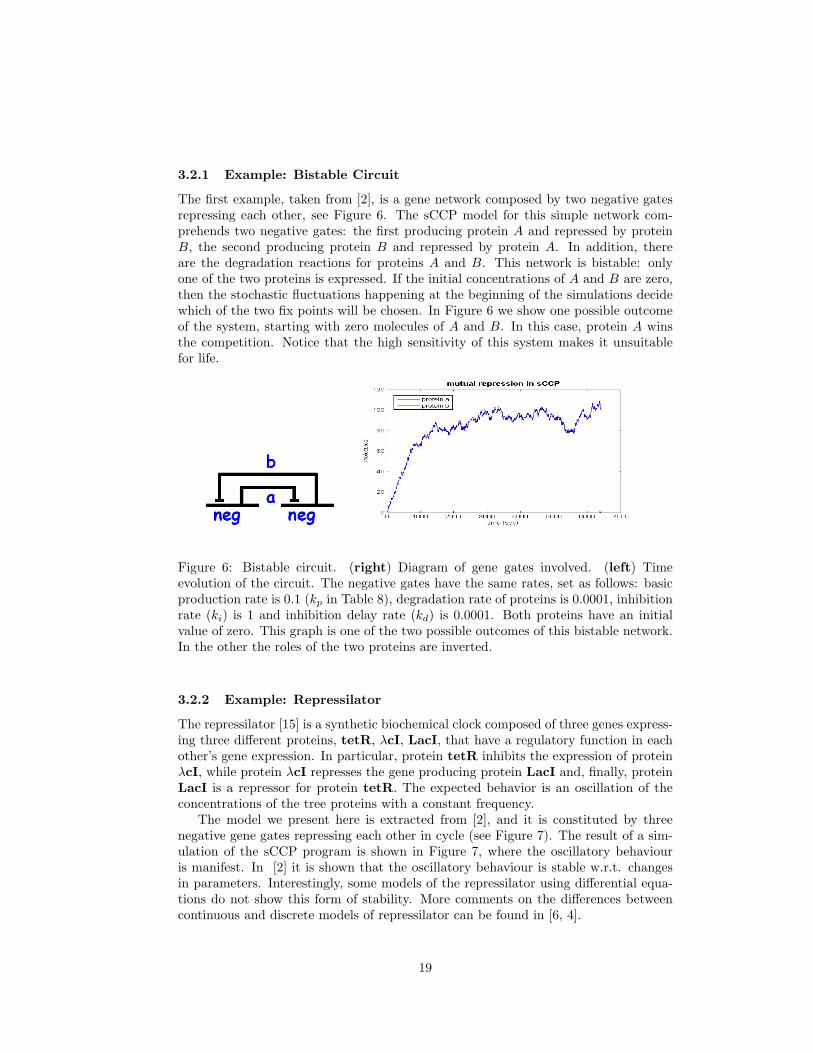
The first example, taken from [2], is a gene network composed by two negative gatesrepressing each other, see Figure 6. The sCCP model for this simple network com-prehends two negative gates: the first producing protein A and repressed by proteinB, the second producing protein B and repressed by protein A. In addition, thereare the degradation reactions for proteins A and B. This network is bistable: onlyone of the two proteins is expressed. If the initial concentrations of A and B are zero,then the stochastic fluctuations happening at the beginning of the simulations decidewhich of the two fix points will be chosen. In Figure 6 we show one possible outcomeof the system, starting with zero molecules of A and B. In this case, protein A winsthe competition. Notice that the high sensitivity of this system makes it unsuitablefor life.

Figure 6: Bistable circuit. (right) Diagram of gene gates involved. (left) Timeevolution of the circuit. The negative gates have the same rates, set as follows: basicproduction rate is 0.1 (kp in Table 8), degradation rate of proteins is 0.0001, inhibitionrate (ki) is 1 and inhibition delay rate (kd) is 0.0001. Both proteins have an initialvalue of zero. This graph is one of the two possible outcomes of this bistable network.In the other the roles of the two proteins are inverted.

3.2.2 Example: Repressilator

The repressilator [15] is a synthetic biochemical clock composed of three genes express-ing three different proteins, tetR, λcI, LacI, that have a regulatory function in eachother’s gene expression. In particular, protein tetR inhibits the expression of proteinλcI, while protein λcI represses the gene producing protein LacI and, finally, proteinLacI is a repressor for protein tetR. The expected behavior is an oscillation of theconcentrations of the tree proteins with a constant frequency.

The model we present here is extracted from [2], and it is constituted by threenegative gene gates repressing each other in cycle (see Figure 7). The result of a sim-ulation of the sCCP program is shown in Figure 7, where the oscillatory behaviouris manifest. In [2] it is shown that the oscillatory behaviour is stable w.r.t. changesin parameters. Interestingly, some models of the repressilator using differential equa-tions do not show this form of stability. More comments on the differences betweencontinuous and discrete models of repressilator can be found in [6, 4].

19

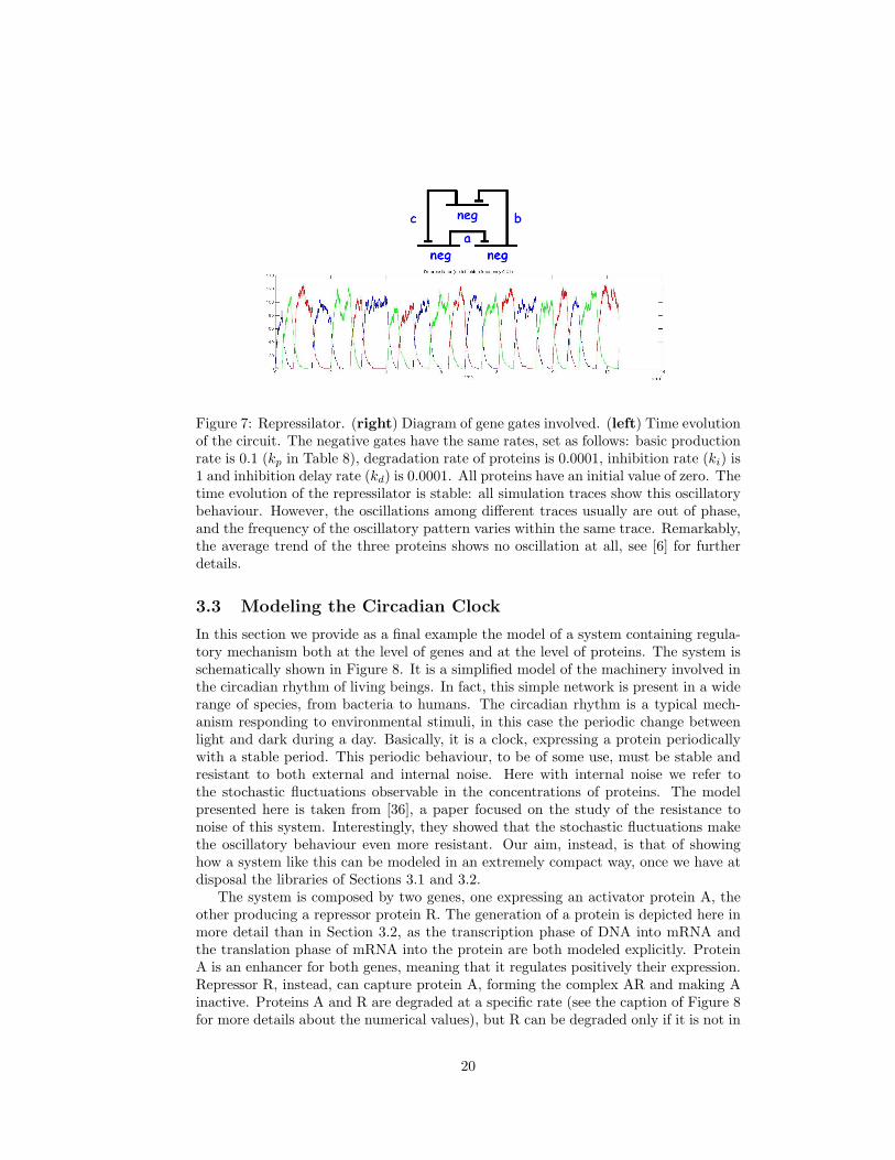
Figure 7: Repressilator. (right) Diagram of gene gates involved. (left) Time evolutionof the circuit. The negative gates have the same rates, set as follows: basic productionrate is 0.1 (kp in Table 8), degradation rate of proteins is 0.0001, inhibition rate (ki) is1 and inhibition delay rate (kd) is 0.0001. All proteins have an initial value of zero. Thetime evolution of the repressilator is stable: all simulation traces show this oscillatorybehaviour. However, the oscillations among different traces usually are out of phase,and the frequency of the oscillatory pattern varies within the same trace. Remarkably,the average trend of the three proteins shows no oscillation at all, see [6] for furtherdetails.

3.3 Modeling the Circadian Clock

In this section we provide as a final example the model of a system containing regula-tory mechanism both at the level of genes and at the level of proteins. The system isschematically shown in Figure 8. It is a simplified model of the machinery involved inthe circadian rhythm of living beings. In fact, this simple network is present in a widerange of species, from bacteria to humans. The circadian rhythm is a typical mech-anism responding to environmental stimuli, in this case the periodic change betweenlight and dark during a day. Basically, it is a clock, expressing a protein periodicallywith a stable period. This periodic behaviour, to be of some use, must be stable andresistant to both external and internal noise. Here with internal noise we refer tothe stochastic fluctuations observable in the concentrations of proteins. The modelpresented here is taken from [36], a paper focused on the study of the resistance tonoise of this system. Interestingly, they showed that the stochastic fluctuations makethe oscillatory behaviour even more resistant. Our aim, instead, is that of showinghow a system like this can be modeled in an extremely compact way, once we have atdisposal the libraries of Sections 3.1 and 3.2.

The system is composed by two genes, one expressing an activator protein A, theother producing a repressor protein R. The generation of a protein is depicted here inmore detail than in Section 3.2, as the transcription phase of DNA into mRNA andthe translation phase of mRNA into the protein are both modeled explicitly. ProteinA is an enhancer for both genes, meaning that it regulates positively their expression.Repressor R, instead, can capture protein A, forming the complex AR and making Ainactive. Proteins A and R are degraded at a specific rate (see the caption of Figure 8for more details about the numerical values), but R can be degraded only if it is not in

20

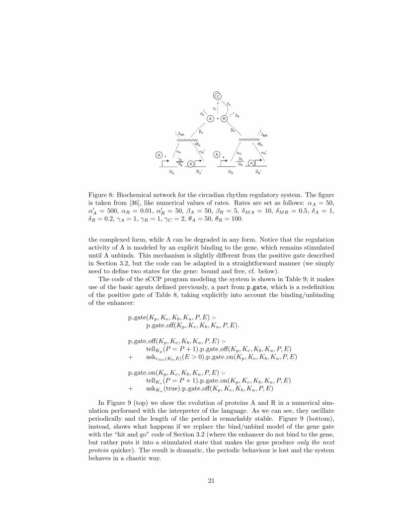
Figure 8: Biochemical network for the circadian rhythm regulatory system. The figureis taken from [36], like numerical values of rates. Rates are set as follows: αA = 50,α′A = 500, αR = 0.01, α′R = 50, βA = 50, βR = 5, δMA = 10, δMR = 0.5, δA = 1,δR = 0.2, γA = 1, γR = 1, γC = 2, θA = 50, θR = 100.

the complexed form, while A can be degraded in any form. Notice that the regulationactivity of A is modeled by an explicit binding to the gene, which remains stimulateduntil A unbinds. This mechanism is slightly different from the positive gate describedin Section 3.2, but the code can be adapted in a straightforward manner (we simplyneed to define two states for the gene: bound and free, cf. below).

The code of the sCCP program modeling the system is shown in Table 9; it makesuse of the basic agents defined previously, a part from p gate, which is a redefinitionof the positive gate of Table 8, taking explicitly into account the binding/unbindingof the enhancer:

p gate(Kp,Ke,Kb,Ku, P, E) :-p gate off(Kp,Ke,Kb,Ku, P, E).

p gate off(Kp,Ke,Kb,Ku, P, E) :-tellKp

(P = P + 1).p gate off(Kp,Ke,Kb,Ku, P, E)+ askrma(Kb,E)(E > 0).p gate on(Kp,Ke,Kb,Ku, P, E)

p gate on(Kp,Ke,Kb,Ku, P, E) :-tellKe(P = P + 1).p gate on(Kp,Ke,Kb,Ku, P, E)

+ askKu(true).p gate off(Kp,Ke,Kb,Ku, P, E)

In Figure 9 (top) we show the evolution of proteins A and R in a numerical sim-ulation performed with the interpreter of the language. As we can see, they oscillateperiodically and the length of the period is remarkably stable. Figure 9 (bottom),instead, shows what happens if we replace the bind/unbind model of the gene gatewith the “hit and go” code of Section 3.2 (where the enhancer do not bind to the gene,but rather puts it into a stimulated state that makes the gene produce only the nextprotein quicker). The result is dramatic, the periodic behaviour is lost and the systembehaves in a chaotic way.

21

pos gate(αA, α′A, γA, θA,MA, A) ‖pos gate(αR, α′R, γR, θR,MR, A) ‖

reaction(βA, [MA], [A]) ‖reaction(δMA, [MA], []) ‖reaction(βR, [MR], [R]) ‖reaction(δMR, [MR], []) ‖

reaction(γC , [A,R], [AR]) ‖reaction(δA, [AR], [R]) ‖

reaction(δA, [A], []) ‖reaction(δR, [R], [])

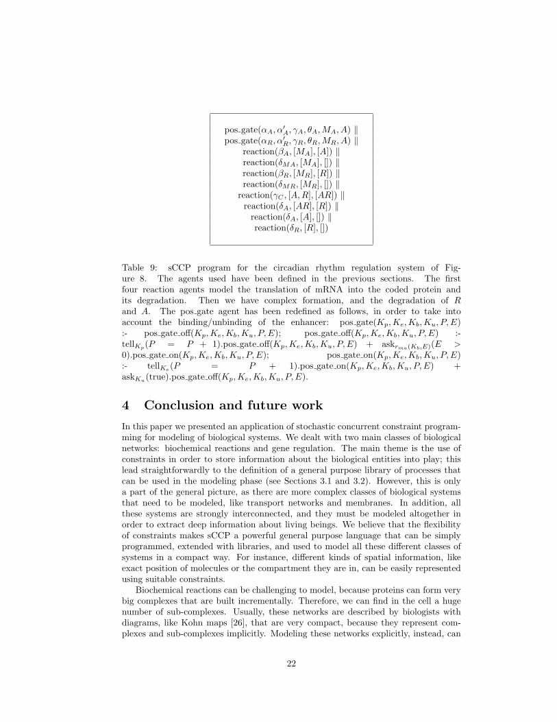
Table 9: sCCP program for the circadian rhythm regulation system of Fig-ure 8. The agents used have been defined in the previous sections. The firstfour reaction agents model the translation of mRNA into the coded protein andits degradation. Then we have complex formation, and the degradation of Rand A. The pos gate agent has been redefined as follows, in order to take intoaccount the binding/unbinding of the enhancer: pos gate(Kp,Ke,Kb,Ku, P, E):- pos gate off(Kp,Ke,Kb,Ku, P, E); pos gate off(Kp,Ke,Kb,Ku, P, E) :-tellKp

(P = P + 1).pos gate off(Kp,Ke,Kb,Ku, P, E) + askrma(Kb,E)(E >0).pos gate on(Kp,Ke,Kb,Ku, P, E); pos gate on(Kp,Ke,Kb,Ku, P, E):- tellKe(P = P + 1).pos gate on(Kp,Ke,Kb,Ku, P, E) +askKu(true).pos gate off(Kp,Ke,Kb,Ku, P, E).

4 Conclusion and future work

In this paper we presented an application of stochastic concurrent constraint program-ming for modeling of biological systems. We dealt with two main classes of biologicalnetworks: biochemical reactions and gene regulation. The main theme is the use ofconstraints in order to store information about the biological entities into play; thislead straightforwardly to the definition of a general purpose library of processes thatcan be used in the modeling phase (see Sections 3.1 and 3.2). However, this is onlya part of the general picture, as there are more complex classes of biological systemsthat need to be modeled, like transport networks and membranes. In addition, allthese systems are strongly interconnected, and they must be modeled altogether inorder to extract deep information about living beings. We believe that the flexibilityof constraints makes sCCP a powerful general purpose language that can be simplyprogrammed, extended with libraries, and used to model all these different classes ofsystems in a compact way. For instance, different kinds of spatial information, likeexact position of molecules or the compartment they are in, can be easily representedusing suitable constraints.

Biochemical reactions can be challenging to model, because proteins can form verybig complexes that are built incrementally. Therefore, we can find in the cell a hugenumber of sub-complexes. Usually, these networks are described by biologists withdiagrams, like Kohn maps [26], that are very compact, because they represent com-plexes and sub-complexes implicitly. Modeling these networks explicitly, instead, can

22

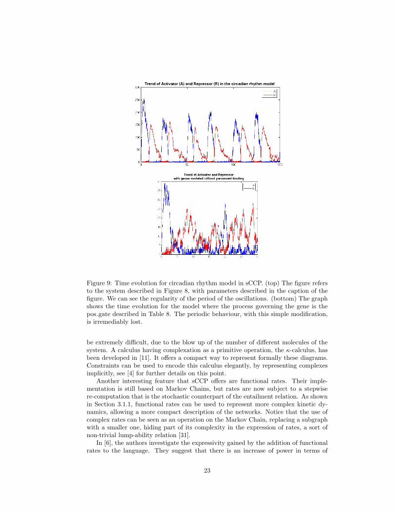
Figure 9: Time evolution for circadian rhythm model in sCCP. (top) The figure refersto the system described in Figure 8, with parameters described in the caption of thefigure. We can see the regularity of the period of the oscillations. (bottom) The graphshows the time evolution for the model where the process governing the gene is thepos gate described in Table 8. The periodic behaviour, with this simple modification,is irremediably lost.

be extremely difficult, due to the blow up of the number of different molecules of thesystem. A calculus having complexation as a primitive operation, the κ-calculus, hasbeen developed in [11]. It offers a compact way to represent formally these diagrams.Constraints can be used to encode this calculus elegantly, by representing complexesimplicitly, see [4] for further details on this point.

Another interesting feature that sCCP offers are functional rates. Their imple-mentation is still based on Markov Chains, but rates are now subject to a stepwisere-computation that is the stochastic counterpart of the entailment relation. As shownin Section 3.1.1, functional rates can be used to represent more complex kinetic dy-namics, allowing a more compact description of the networks. Notice that the use ofcomplex rates can be seen as an operation on the Markov Chain, replacing a subgraphwith a smaller one, hiding part of its complexity in the expression of rates, a sort ofnon-trivial lump-ability relation [31].

In [6], the authors investigate the expressivity gained by the addition of functionalrates to the language. They suggest that there is an increase of power in terms of

23

dynamical behaviours that can be reproduced, after encoding in sCCP a wide class ofdifferential equations. This problem, together with the inverse one of describing sCCPprograms by differential equations, is an interesting direction of research, which maylead to an integration of these different techniques, see [23, 6, 4] for further comments.

Finally, we plan to implement a more powerful and fast interpreter for the lan-guage, using also all available tricks to increase the speed of stochastic simulations [18].Moreover, we plan to tackle also the problem of distributing efficiently the stochasticsimulations of programs written in sCCP.

References

[1] R. Alur, C. Belta, F. Ivancic, V. Kumar, M. Mintz, G. Pappas, H. Rubin, andJ. Schug. Hybrid modeling and simulation of biomolecular networks. In Pro-ceedings of Fourth International Workshop on Hybrid Systems: Computation andControl, volume LNCS 2034, pages 19–32, 2001.

[2] R. Blossey, L. Cardelli, and A. Phillips. A compositional approach to the stochas-tic dynamics of gene networks. T. Comp. Sys. Biology, pages 99–122, 2006.

[3] L. Bortolussi. Stochastic concurrent constraint programming. In Proceedings of4th International Workshop on Quantitative Aspects of Programming Languages,QAPL 2006, ENTCS, volume 164, pages 65–80, 2006.

[4] L. Bortolussi. Constraint-based approaches to stochastic dynamics of biologicalsystems. PhD thesis, PhD in Computer Science, University of Udine, 2007. Inpreparation. Available on request from the author.

[5] L. Bortolussi and A. Policriti. Modeling biological systems in concurrent con-straint programming. In Proceedings of Second International Workshop onConstraint-based Methods in Bioinformatics, WCB 2006, 2006.

[6] L. Bortolussi and A. Policriti. Relating stochastic process algebras and differentialequations for biological modeling. Proceedings of PASTA 2006, 2006.

[7] J. M. Bower and H. Bolouri eds. Computational Modeling of Genetic and Bio-chemical Networks. MIT Press, Cambridge, 2000.

[8] L. Cardelli. Abstract machines of systems biology. Transactions on ComputationalSystems Biology, III, LNBI 3737:145–168, 2005.

[9] L. Cardelli and A. Phillips. A correct abstract machine for the stochastic pi-calculus. In Proceeding of Bioconcur 2004, 2004.

[10] A. Cornish-Bowden. Fundamentals of Chemical Kinetics. Portland Press, 3rdedition, 2004.

[11] V. Danos and C. Laneve. Formal molecular biology. Theor. Comput. Sci.,325(1):69–110, 2004.

[12] F.S. de Boer, A. Di Pierro, and C. Palamidessi. Nondeterminism and infinitecomputations in constraint programming. Theoretical Computer Science, 151(1),1995.

24

[13] H. De Jong. Modeling and simulation of genetic regulatory systems: A literaturereview. Journal of Computational Biology, 9(1):67–103, 2002.

[14] L. Edelstein-Keshet. Mathematical Models in Biology. SIAM, 2005.

[15] M.B. Elowitz and S. Leibler. A syntetic oscillatory network of transcriptionalregulators. Nature, 403:335–338, 2000.

[16] Swedish Institute for Computer Science. Sicstus prolog home page.

[17] D. Gillespie. The chemical langevin equation. Journal of Chemical Physics,113(1):297–306, 2000.

[18] D. Gillespie and L. Petzold. System Modelling in Cellular Biology, chapter Nu-merical Simulation for Biochemical Kinetics. MIT Press, 2006.

[19] D. T. Gillespie. A rigorous derivation of the chemical master equation. PhysicaA, 22:403–432, 1992.

[20] D.T. Gillespie. A general method for numerically simulating the stochastic timeevolution of coupled chemical reactions. J. of Computational Physics, 22, 1976.

[21] D.T. Gillespie. Exact stochastic simulation of coupled chemical reactions. J. ofPhysical Chemistry, 81(25), 1977.

[22] L. Henkin, J.D. Monk, and A. Tarski. Cylindric Algebras, Part I. North-Holland,Amsterdam, 1971.

[23] J. Hillston. Fluid flow approximation of pepa models. In Proceedings of the SecondInternational Conference on the Quantitative Evaluation of Systems (QEST05),2005.

[24] C.F. Huang and J.T. Ferrell. Ultrasensitivity in the mitogen-activated proteinkinase cascade. PNAS, Biochemistry, 151:10078–10083, 1996.

[25] H. Kitano. Foundations of Systems Biology. MIT Press, 2001.

[26] K. W. Kohn. Molecular interaction map of the mammalian cell cycle control anddna repair systems. Molecular Biology of the Cell, 10:2703–2734, August 1999.

[27] J. R. Norris. Markov Chains. Cambridge University Press, 1997.

[28] C. Priami. Stochastic π-calculus. The Computer Journal, 38(6):578–589, 1995.

[29] C. Priami and P. Quaglia. Modelling the dynamics of biosystems. Briefings inBioinformatics, 5(3):259–269, 2004.

[30] C. Priami, A. Regev, E. Y. Shapiro, and W. Silverman. Application of a stochasticname-passing calculus to representation and simulation of molecular processes.Inf. Process. Lett., 80(1):25–31, 2001.

[31] C. V. Rao and A. P. Arkin. Stochastic chemical kinetics and the quasi-steadystate assumption: Application to the gillespie algorithm. Journal of ChemicalPhysics, 118(11):4999–5010, March 2003.

25

[32] A. Regev and E. Shapiro. Cellular abstractions: Cells as computation. Nature,419, 2002.

[33] V. A. Saraswat. Concurrent Constraint Programming. MIT press, 1993.

[34] V. A. Saraswat, M. Rinard, and P. Panangaden. Semantics foundations of con-current constraint programming. In Proceedings of POPL, 1991.

[35] B. E. Shapiro, A. Levchenko, E. M. Meyerowitz, Wold B. J., and E. D. Mjolsness.Cellerator: extending a computer algebra system to include biochemical arrowsfor signal transduction simulations. Bioinformatics, 19(5):677–678, 2003.

[36] J. M. G. Vilar, H. Yuan Kueh, N. Barkai, and S. Leibler. Mechanisms of noiseresistance in genetic oscillators. PNAS, 99(9):5991, 2002.

[37] Darren J. Wilkinson. Stochastic Modelling for Systems Biology. Chapman & Hall,2006.

26