Modeling auditory processing and speech perception in ... · Modeling auditory processing and...

General rights Copyright and moral rights for the publications made accessible in the public portal are retained by the authors and/or other copyright owners and it is a condition of accessing publications that users recognise and abide by the legal requirements associated with these rights.

Users may download and print one copy of any publication from the public portal for the purpose of private study or research.

You may not further distribute the material or use it for any profit-making activity or commercial gain

You may freely distribute the URL identifying the publication in the public portal If you believe that this document breaches copyright please contact us providing details, and we will remove access to the work immediately and investigate your claim.

Downloaded from orbit.dtu.dk on: May 26, 2020

Modeling auditory processing and speech perception in hearing-impaired listeners

Jepsen, Morten Løve

Publication date:2010

Document VersionPublisher's PDF, also known as Version of record

Link back to DTU Orbit

Citation (APA):Jepsen, M. L. (2010). Modeling auditory processing and speech perception in hearing-impaired listeners.Technical University of Denmark.

https://orbit.dtu.dk/en/publications/1f755de6-43c6-4732-9e1b-88325e6530bd

Morten Løve Jepsen

CONTRIBUTIONS TO HEARING RESEARCH Volume 7

Modeling auditory processing and speech perception in hearing-impaired listeners

i

i

“MainFile” — 2010/7/15 — 15:31 — page i — #1i

i

i

i

i

i

Modeling auditory processing

and speech perception in

hearing-impaired listeners

Ph.D. thesis by

Morten Løve Jepsen

Technical University of Denmark2010

i

i

“MainFile” — 2010/7/15 — 15:31 — page ii — #2i

i

i

i

i

i

c© Morten Løve Jepsen, 2010

Printed in Denmark by Rosendahls - Schultz Grafisk A/S.

The defense was held on May 27, 2010.

i

i

“MainFile” — 2010/7/15 — 15:31 — page iii — #3i

i

i

i

i

i

Denne ph.d.-afhandling er indleveret til bedømmelse til Institut forElektroteknologi på Danmarks Tekniske Universitet.

Projektet er hovedsageligt udført hos Center for anvendt høreforskn-ing, Institut for Elektroteknologi på Danmarks Tekniske Universitet.Dele af projektet er udført på Hearing Research Center ved BostonUniversity, Massachusetts, USA.

Vejledere:

Hovedvejleder:Professor Torsten DauCenter for anvendt høreforskning, DTU ElektroLyngby, Danmark

Medvejledere:Lars Bramsløw, Ph.D. and Michael S. Pedersen, Ph.D.OticonSmørum, Danmark

Vejleder på delprojekt på Boston University:Dr. Oded GhitzaHearing Research Center, Boston UniversityBoston, Massachusetts, USA

Finansiering:

Projektet var finansieret gennem Oticon Fonden, Forskerskolen SNAK (Sanser,nerver, adfærd og kommunikation) og Ministeriet for videnskab, teknologi ogudvikling.

Et eksternt forskningsophold blev endvidere støttet af Oticon Fonden, Otto MønstedsFond og Kaj og Hermilla Ostenfeld’s Fond.

4. Februar, 2010

.

Morten Løve Jepsen, forfatter

i

i

“MainFile” — 2010/7/15 — 15:31 — page iv — #4i

i

i

i

i

i

i

i

“MainFile” — 2010/7/15 — 15:31 — page v — #5i

i

i

i

i

i

To my sonTobias

i

i

“MainFile” — 2010/7/15 — 15:31 — page vi — #6i

i

i

i

i

i

i

i

“MainFile” — 2010/7/15 — 15:31 — page vii — #7i

i

i

i

i

i

Abstract

A better understanding of how the human auditory system represents and analyzessounds and how hearing impairment affects such processing is of great interest forresearchers in the fields of auditory neuroscience, audiology, and speech communica-tion as well as for applications in hearing-instrument and speech technology. In thisthesis, the primary focus was on the development and evaluation of a computationalmodel of human auditory signal-processing and perception.The model was initiallydesigned to simulate the normal-hearing auditory system with particular focus onthe nonlinear processing in the inner ear, or cochlea. The model was shown toaccount for various aspects of spectro-temporal processing and perception in tasks ofintensity discrimination, tone-in-noise detection, forward masking, spectral maskingand amplitude modulation detection. Secondly, a series of experiments was performedaimed at experimentally characterizing the effects of cochlear damage on listeners’auditory processing, in terms of sensitivity loss and reduced temporal and spectralresolution. The results showed that listeners with comparable audiograms canhave very different estimated cochlear input-output functions, frequency selectivity,intensity discrimination limens and effects of simultaneous- and forward masking.Part of the measured data was used to adjust the parameters ofthe stages in the model,that simulate the cochlear processing. The remaining data were used to evaluate thefitted models. It was shown that an accurate simulation of cochlear input-outputfunctions, in addition to the audiogram, played a major rolein accounting both forsensitivity and supra-threshold processing. Finally, themodel was used as a front-end in a framework developed to predict consonant discrimination in a diagnosticrhyme test. The framework was constructed such that discrimination errors originatingfrom the front-end and the back-end were separated. The front-end was fitted toindividual listeners with cochlear hearing loss accordingto non-speech data, andspeech data were obtained in the same listeners. It was shownthat most observationsin the measured consonant discrimination error patterns were predicted by the model,although error rates were systematically underestimated by the model in few particularacoustic-phonetic features. These results reflect a relation between basic auditoryprocessing deficits and reduced speech perception performance in the listeners withcochlear hearing loss. Overall, this work suggests a possible explanation of thevariability in consequences of cochlear hearing loss. The proposed model might be aninteresting tool for, e.g., evaluation of hearing-aid signal processing.

vii

i

i

“MainFile” — 2010/7/15 — 15:31 — page viii — #8i

i

i

i

i

i

i

i

“MainFile” — 2010/7/15 — 15:31 — page ix — #9i

i

i

i

i

i

Resumé

Der er stor interesse for en bedre forståelse af hvordan menneskets hørelse analysererog repræsenterer lyde og for at forstå hvordan høretab påvirker signalbehandlingenog opfattelsen af lyd. Disse aspekter er særligt interessante for forskere indenforneurovidenskab, audiologi, talekommunikation og i anvendelsesområder som ihøreapparats og tale-teknologi. Det primære fokus i denne afhandling var udviklingog evaluering af en beregningsmodel for auditiv signalbehandling og lydopfattelse hosmennesker. Modellen blev først udviklet til at simulere detnormalthørende auditivesystem med fokus på den ikke-lineære processering i det indre øre (cochlea). Det blevvist, at modellen kunne forklare aspekter der vedrører spektro-temporal processering,såsom intensitets-diskrimination, detektering af toner istøj, tids-maskering (forwardmasking), spektral maskering samt detektering af amplitude-modulation. Dernæstblev det undersøgt hvordan man ved hjælp af psykoakustiske eksperimenter kankarakterisere den auditive signalbehandling hos hørehæmmede med høretab i detindre øre. Disse eksperimenter testede hørbarhed samt eventuelt reduceret opløsningi tid og frekvens. Resultaterne viste at personer med sammenlignelige audiogrammerhavde vidt forskellige udfald i forhold input-output funktioner i cochlea, frekvens-selektivitet, intensitets-diskrimination samt simultanmaskering og tids-maskering.En del af data blev brugt til at tilpasse parametre i de trin i modellen der simulererdet indre øres funktion og formålet var at beskrive signalbehandlingen hos de målteindivider. De resterende data blev brugt til at evaluere de tilpassede modeller. Udoveraudiogrammet, viste det sig at være vigtigt at kunne simulere cochlear processeringenpræcist for at kunne beskrive både hørbarhed og såkaldt “supra-tærskel” processering.Til sidst blev modellen brugt som “front-end” i et talegenkendelses-system målrettetmod at kunne forudsige data fra et specifikt taleeksperiment(diagnostic rhyme test).Systemet var udviklet til at kunne separere konsonant-diskriminations fejl i forholdtil om de stammede fra modellens front-end eller detektor (back-end). Modellensfront-end blev på baggrund af maskeringsdata tilpasset tilpersoner med høretabi det indre øre, og fejlrater i tale-eksperimentet blev målti de samme personer.Modellen kunne i de fleste betingelser forudsige mønsteret ide målte konsonant-diskriminations fejl. Disse resultater afspejler at der eren sammenhæng mellem denforringede signalbehandling i hørelsen og forværret taleopfattelse hos hørehæmmede.

ix

i

i

“MainFile” — 2010/7/15 — 15:31 — page x — #10i

i

i

i

i

i

x

Samlet set bliver der i denne afhandling foreslået en række mulige forklaringer påvariationen i hørehæmmedes lydopfattelse. Derudover kan den foreslåede modelmuligvis være interessant i anvendelse som et værktøj, eksempelvis til at evalueresignalbehandlingen i høreapparater.

i

i

“MainFile” — 2010/7/15 — 15:31 — page xi — #11i

i

i

i

i

i

Forord

Det er min overbevisning, at tiden går hurtigt hvis man nyderhvad man laver. Det ernetop hvad der er sket for mig i de sidste 3 år. Det har været en fornøjelse at mødepå arbejde hver dag i forbindelse med dette projekt. Den primære årsag har vært demennesker som har omgivet mig på kontoret og privat.

Jeg takker Torsten Dau for at have været min inspiration til at gå i gang med etforskningsprojekt. Hans engagement og den energi han har lagt i vejledningen eruvurderlig. Måden hvorpå han involverer sig som kollega og ven har gjort det til enfornøjelse at arbejde på projektet.

Adskillige folk og medstuderende har skabt et enestående arbejdsmiljø på Center foranvendt høreforskning (CAHR), både fagligt og socialt. Forat nævne nogle få: Claus,Eric, Filip, Iris, Olaf, Sarah, Sebastien, Sylvain og Tobias... Tak. Også en tak tilMartin, Sven og Anders for nogle underholdende timer i pauserne.

Jeg er taknemmelig overfor min familie, især mine forældre.I har været en uundværligstøtte, og jeg havde ikke kunne udføre dette arbejde uden jeres hjælp og fleksibilitet.

Mine medvejledere hos Oticon, Lars og Michael, har vist storinteresse i projektetsforløb, og var en stor hjælp i projektet indledende fase i forhold til planlægning og tilat vælge en indholdsmæssig relevant retning.

The people at Boston University were very welcoming, and made my visit in Bostonduring the fall of 2008 a great experience from day one. Thankyou, Oded and Steve.

Tak til alle forsøgspersonerne der har deltaget i mine lytteforsøg. Resultaterne framålingerne er selvfølgelig en vigtig del af hele projektet.

Og mest af alle vil jeg takke min søn, Tobias, for alle de dejlige dage som har fjernetmine tanker fra arbejdet når det var nødvendigt. Disse år havde ikke været så sjove oglykkelige uden dig.

Morten Løve Jepsen, 4. februar, 2010

xi

i

i

“MainFile” — 2010/7/15 — 15:31 — page xii — #12i

i

i

i

i

i

i

i

“MainFile” — 2010/7/15 — 15:31 — page xiii — #13i

i

i

i

i

i

List of publications

Journal articles:

Jepsen, M. L., Ewert, S. D. and Dau, T.(2008), ”A computational model of humanauditory signal processing and perception”, J. Acoust. Soc. Am. 124, 422-438.

Moore, B. C. J., Glasberg, B. R., and Jepsen, M. L.(2009), ”Effects of pulsing ofthe target tone on the audibility of partials in inharmonic complex tones”, J. Acoust.Soc. Am. 125, 3194-3204.

Jepsen, M. L., and Dau, T.(2010), “Characterizing auditory processing andperception in individual listeners with sensorineural hearing loss”, J. Acoust. Soc.Am., Submitted.

Conference articles:

Dau, T., Jepsen, M. L., and Ewert, S. D.(2007), ”Modeling spectral and temporalmasking in the human auditory system”, Proceedings of the 19th InternationalCongress on Acoustics, ICA ’07, Madrid, Spain.

Dau, T., Jepsen, M. L., and Ewert, S. D.(2008), ”Spectral and temporal processingin the human auditory system”, Proceedings of the International Symposium onAuditory and Audiological Research (ISAAR), Helsingør, Denmark.

Jepsen, M. L., and Dau, T.(2008), ”Modeling auditory signal processing in hearing-impaired listeners”, Proceedings of the International Symposium on Auditory andAudiological Research (ISAAR), Helsingør, Denmark.

Jepsen, M. L., and Dau, T.(2010), ”Modeling a damaged cochlea: beyond non-speech psychophysics”, International Symposium on Auditory and AudiologicalResearch (ISAAR), Helsingør, Denmark.Submitted.

Published abstracts:

Jepsen, M. L., and Dau, T.(2008), ”Estimating the basilar-membrane input-outputfunction in normal-hearing and hearing-impaired listeners using forward masking”,J. Acoust. Soc. Am. 123, 3859. Acoustics ’08, Paris, France.

Jepsen, M. L., and Dau, T.(2008), ”Modeling auditory perception of individualhearing-impaired listeners”, International Hearing Aid Research Conference (IH-CON), Lake Tahoe, CA, USA.

Dau, T. and Jepsen, M. L.(2010), ”Modeling Individual Hearing Impairment witha Physiologically-Based Auditory Perception Model”, Association for Research inOtolaryngology (ARO), Midwinter Meeting, February 2010, Anaheim, CA, USA.

i

i

“MainFile” — 2010/7/15 — 15:31 — page xiv — #14i

i

i

i

i

i

i

i

“MainFile” — 2010/7/15 — 15:31 — page xv — #15i

i

i

i

i

i

Contents

List of abbreviations xix

1 General introduction 1

2 A computational model of human auditory signal processing

and perception 7

2.1 Introduction. . . . . . . . . . . . . . . . . . . . . . . . . . . . . . . 8

2.2 Description of the model. . . . . . . . . . . . . . . . . . . . . . . . 14

2.2.1 Overall structure. . . . . . . . . . . . . . . . . . . . . . . . 14

2.2.2 Processing stages in the model. . . . . . . . . . . . . . . . . 14

2.3 Experimental method. . . . . . . . . . . . . . . . . . . . . . . . . . 22

2.3.1 Subjects. . . . . . . . . . . . . . . . . . . . . . . . . . . . . 22

2.3.2 Apparatus and procedure. . . . . . . . . . . . . . . . . . . . 22

2.3.3 Stimuli . . . . . . . . . . . . . . . . . . . . . . . . . . . . . 23

2.3.4 Simulation parameters. . . . . . . . . . . . . . . . . . . . . 25

2.4 Results. . . . . . . . . . . . . . . . . . . . . . . . . . . . . . . . . . 27

2.4.1 Intensity discrimination . . . . . . . . . . . . . . . . . . . . 27

2.4.2 Tone-in-noise simultaneous masking. . . . . . . . . . . . . . 28

2.4.3 Spectral masking patterns with narrowband signals and maskers30

2.4.4 Forward masking with noise and on- versus off-frequency

tone maskers. . . . . . . . . . . . . . . . . . . . . . . . . . 34

2.4.5 Modulation detection with noise carriers of different bandwidth 38

2.5 Discussion. . . . . . . . . . . . . . . . . . . . . . . . . . . . . . . . 41

xv

i

i

“MainFile” — 2010/7/15 — 15:31 — page xvi — #16i

i

i

i

i

i

xvi

2.5.1 Role of nonlinear cochlear processing in auditory masking . . 41

2.5.2 Effects of other changes in the processing on the overall model

performance . . . . . . . . . . . . . . . . . . . . . . . . . . 44

2.5.3 Limitations of the model. . . . . . . . . . . . . . . . . . . . 46

2.5.4 Perspectives. . . . . . . . . . . . . . . . . . . . . . . . . . . 47

2.6 Summary . . . . . . . . . . . . . . . . . . . . . . . . . . . . . . . . 49

2.7 Appendix: DRNL parameters of the model. . . . . . . . . . . . . . . 50

3 Estimating basilar-membrane input-output functions

using forward masking 51

3.1 Introduction. . . . . . . . . . . . . . . . . . . . . . . . . . . . . . . 52

3.2 Experimental methods. . . . . . . . . . . . . . . . . . . . . . . . . 58

3.2.1 Listeners . . . . . . . . . . . . . . . . . . . . . . . . . . . . 58


3.2.3 Stimuli . . . . . . . . . . . . . . . . . . . . . . . . . . . . . 59

3.3 Results. . . . . . . . . . . . . . . . . . . . . . . . . . . . . . . . . . 61

3.3.1 BM I/O functions in NH listeners. . . . . . . . . . . . . . . 61

3.3.2 BM I/O functions in HI listeners. . . . . . . . . . . . . . . . 63

3.4 Discussion. . . . . . . . . . . . . . . . . . . . . . . . . . . . . . . . 69

3.5 Conclusions. . . . . . . . . . . . . . . . . . . . . . . . . . . . . . . 72

3.6 Appendix: Additional information about the listeners. . . . . . . . . 73

4 Characterizing auditory processing and perception in individual

listeners with sensorineural hearing loss 75

4.1 Introduction. . . . . . . . . . . . . . . . . . . . . . . . . . . . . . . 76

4.2 Auditory processing model. . . . . . . . . . . . . . . . . . . . . . . 82

4.2.1 Stages of the auditory processing. . . . . . . . . . . . . . . 83

4.2.2 Parameter changes to account for SNHL. . . . . . . . . . . . 85

4.3 Experimental method. . . . . . . . . . . . . . . . . . . . . . . . . . 88

4.3.1 Test subjects. . . . . . . . . . . . . . . . . . . . . . . . . . 88

i

i

“MainFile” — 2010/7/15 — 15:31 — page xvii — #17i

i

i

i

i

i

xvii


4.3.3 Stimuli . . . . . . . . . . . . . . . . . . . . . . . . . . . . . 89

4.4 Results. . . . . . . . . . . . . . . . . . . . . . . . . . . . . . . . . . 94

4.4.1 BM input-output functions. . . . . . . . . . . . . . . . . . . 94

4.4.2 Predicted pure-tone audiograms. . . . . . . . . . . . . . . . 101

4.4.3 Relation between pure-tone threshold and estimates of com-

pression, HLOHC and HLIHC . . . . . . . . . . . . . . . . . . 101

4.4.4 Frequency selectivity. . . . . . . . . . . . . . . . . . . . . . 102

4.4.5 Simultaneous- and forward masking. . . . . . . . . . . . . . 107

4.4.6 Intensity discrimination . . . . . . . . . . . . . . . . . . . . 110

4.5 Discussion. . . . . . . . . . . . . . . . . . . . . . . . . . . . . . . . 115

4.5.1 Behavioral estimates of human BM input/output functions . . 115

4.5.2 Evaluation of the models fitted to individuals. . . . . . . . . 118

4.5.3 Relationships between different measures in individual listeners119

4.5.4 Capabilities and limitations of the modeling approach . . . . . 119

4.5.5 Perspectives. . . . . . . . . . . . . . . . . . . . . . . . . . . 124

4.6 Conclusions. . . . . . . . . . . . . . . . . . . . . . . . . . . . . . . 125

4.7 Appendix: Additional information about the listeners. . . . . . . . . 126

5 Relating individual consonant confusions to

auditory processing in listeners with cochlear damage 129

5.1 Introduction. . . . . . . . . . . . . . . . . . . . . . . . . . . . . . . 130

5.2 Experimental methods. . . . . . . . . . . . . . . . . . . . . . . . . 135

5.2.1 Listeners . . . . . . . . . . . . . . . . . . . . . . . . . . . . 135

5.2.2 Apparatus. . . . . . . . . . . . . . . . . . . . . . . . . . . . 136

5.2.3 Temporal masking curves (TMC). . . . . . . . . . . . . . . 136

5.2.4 The diagnostic rhyme test (DRT). . . . . . . . . . . . . . . . 136

5.3 Modeling speech perception. . . . . . . . . . . . . . . . . . . . . . 139

5.3.1 The front end. . . . . . . . . . . . . . . . . . . . . . . . . . 139

5.3.2 Simulation of individual hearing loss. . . . . . . . . . . . . 139

i

i

“MainFile” — 2010/7/15 — 15:31 — page xviii — #18i

i

i

i

i

i

xviii

5.3.3 Internal representation of the stimuli after auditory processing 141

5.3.4 The back end. . . . . . . . . . . . . . . . . . . . . . . . . . 143

5.4 Results. . . . . . . . . . . . . . . . . . . . . . . . . . . . . . . . . . 149

5.4.1 Characterizing individual hearing impairment usingnon-

speech stimuli . . . . . . . . . . . . . . . . . . . . . . . . . 149

5.4.2 DRT error patterns. . . . . . . . . . . . . . . . . . . . . . . 155

5.5 Discussion. . . . . . . . . . . . . . . . . . . . . . . . . . . . . . . . 164

5.5.1 Front-end processing. . . . . . . . . . . . . . . . . . . . . . 164

5.5.2 Back-end processing. . . . . . . . . . . . . . . . . . . . . . 165

5.5.3 Limitations of the approach. . . . . . . . . . . . . . . . . . 166

5.6 Conclusions. . . . . . . . . . . . . . . . . . . . . . . . . . . . . . . 168

6 General discussion 169

References 173

i

i

“MainFile” — 2010/7/15 — 15:31 — page xix — #19i

i

i

i

i

i

List of abbreviations

AM Amplitude modulation

AN Auditory nerve

BM Basilar membrane

CASP Computational Auditory Signal-processing and Perception

CF Characteristic frequency

CM Compactness

DRNL Dual-resonance nonlinear

DRT Diagnostic rhyme test

ERB Equivalent rectangular bandwidth

GOM Growth-of-masking

GV Graveness

HI Hearing impaired

HL Hearing level

HLTOT Total hearing loss

HLOHC Hearing loss due to outer hair-cell loss

HLIHC Hearing loss due to inner hair-cell loss

IHC Inner hair cell

I/O Input-output

IR Internal representation

JND Just noticeable difference

xix

i

i

“MainFile” — 2010/7/15 — 15:31 — page xx — #20i

i

i

i

i

i

xx

MSE Mean squared error

MSI Masker-signal interval

NH Normal hearing

NN Noise signal and noise masker

NS Nasality

NT Noise signal and tone masker

OHC Outer hair cell

rms Root-mean-square

roex Rounded exponential

SAM Sinusoidally amplitude modulated

SB Sibilation

SD Standard deviation

SL Sensation level

SNHL Sensorineural hearing loss

SNR Signal-to-noise ratio

SPL Sound pressure level

SRT Speech reception threshold

ST Sustention

TFS Temporal fine structure

TMC Temporal masking curve

TMTF Temporal modulation transfer function

TN Tone signal and noise masker

TT Tone signal and tone masker

VC Voicing

i

i

“MainFile” — 2010/7/15 — 15:31 — page 1 — #21i

i

i

i

i

i

1General introduction

Hearing loss affects the life of millions of people throughout the world. The increasing

population of elderly people and the present day noise exposure of young people

are likely to further increase the number of people with hearing impairment (HI)

over the next years. Impaired hearing ability has major consequences for every-day

life, since acoustic communication is a primary source of information. Hearing-aid

technology has experienced a great evolution in the last decades, and modern hearing

aids undoubtedly help a large part of the HI people to restoretheir ability to function

in every-day situations. However, the performances in day-to-day tasks which involve

hearing, e.g., understanding an acoustic message or speechin a noisy environment,

vary substantially among hearing-aid users. Some experience more benefit than

others.

There has been extensive research on understanding the function of hearing and

how the human auditory system analyzes acoustic signals. A lot has been learned over

the years but many aspects still remain unclear. The normally functioning auditory

system has an impressive capability to extract informationfrom a mixture of sounds

from an acoustic environment. The challenges are to identify a sound source and

disregard the irrelevant information, while still being attentive to new potentially

important acoustic events. Psychoacoustic measurements are usually used in research

on the processing in the human auditory systems. Several experiments, such as

the measurement of signal-detection thresholds in the presence of a masker, have

been developed to gain insight into basic auditory function. For example, notched-

noise masking and forward masking have typically been used to measure the spectral

and temporal resolution of the system, respectively. The aim of models of auditory

processing and perception has been to match the human performance in tasks like

these.

1

i

i

“MainFile” — 2010/7/15 — 15:31 — page 2 — #22i

i

i

i

i

i

2 1. General introduction

Computer models of the auditory system become more complex the more we

understand about the underlying mechanisms of hearing, andthe models can account

for several fundamental aspects when simulating the performances of humans in

certain tasks. However, there is still room for substantialimprovement, especially

regarding generalized models that can account for a broad variety of data. Most

existing models can be expected to simulate the particular aspects which they were

specifically designed for. For example, models that have focused on the simulation of

precise temporal processing in the auditory periphery are not necessarily successful

when considering the auditory spectral analysis.

The signal processing of the inner ear, the cochlea, and in particular the basilar

membrane (BM) is of great importance for understanding the capability of the auditory

periphery to process complex sounds. The BM basically realizes a frequency analyzer

which is highly nonlinear and has level-dependent compression. This feature partly

explains our ability to perceive a wide dynamic range of input sound pressure levels

which allows the subsequent neural system that has a very limited dynamic range to

further process the incoming information. The nonlinearity has several consequences

on spectro-temporal auditory processing. The sharpness ofthe auditory filters reflects

the ability of frequency selectivity, and their bandwidthsare level-dependent. The

cochlea also realizes a nonlinear gain which effectively amplifies low-level input

signals. It thus seems that an appropriate simulation of theprocessing on the BM

is a key element in a successful model of the auditory system.

The most typical type of hearing loss is the so-called sensorineural hearing loss

(SNHL), which is a consequence of a dysfunction of sensory hair-cells within the

cochlea. A typical consequence of hair-cell loss is an abnormal BM processing.

Although there are substantial individual differences among the people with this

type of hearing loss, the nonlinear gain is typically reduced. Changes in the

compressive behavior of the BM affect the tuning of the auditory filters, which have

been observed to be broader in listeners with SNHL. Such effects have dramatic

perceptual consequences for the HI listeners, since their ability to resolve sounds

in time and frequency is degraded. Individual differences in the basic auditory

processing may explain the variability in the severity of communication problems

across HI listeners as well as the varying benefit from compensation by hearing-

i

i

“MainFile” — 2010/7/15 — 15:31 — page 3 — #23i

i

i

i

i

i

3

aids. It is likely that an individual characterization of cochlear processing is important

for a better understanding of the perceptual consequences of cochlear damage or

SNHL. Such characterization needs a set of critical experiments, psychoacoustic

or objective measures, and provides an "auditory profile" for each individual HI

listener, including substantial information in addition to the conventional audiogram.

Auditory processing models of individual hearing loss may be particularly interesting

for the evaluation of novel hearing-aid processing and compensation strategies, or the

prediction of implications of hearing loss on speech intelligibility and sound quality.

The most serious consequence of hearing loss is probably thereduced ability to

understand speech information in noisy backgrounds or in conditions with multiple

speech sources. This has often been referred to as the "cocktail party problem".

Psychoacoustic measures of speech intelligibility typically estimate the signal-to-

noise ratio (SNR) at which a pre-defined amount of words, presented in a masking

condition, is correctly identified. This is reflected in measures of the speech reception

threshold (SRT), hence it reflects an average long-term performance. Other behavioral

measures of speech perception extract more detailed information about specific speech

recognition errors. For example, measures of consonant identification in noise provide

detailed consonant confusion patterns. It is likely that there is a relation between these

speech measures and the outcomes of the non-speech psychophysics described earlier.

A computational model which appropriately simulates the processing in normal-

hearing (NH) and HI listeners and further includes an appropriate "central operator",

such as an optimal detector or a recognizer, would provide a very powerful tool to

explain the observed variation in the data, particularly among the HI listeners. The

work presented in this thesis attempted to provide a step in this direction in addition

to the capability to explain non-speech data.

This thesis presents the results of four interconnected studies. InChapter 2,

a model of computational auditory signal processing and perception (CASP) is

described. It was developed to account for a variety of masking and discrimination

data by simulating the monaural signal processing of the normally-functioning

auditory system. It represents a further development of an existing model of auditory

processing and the major modifications addressed the nonlinear cochlear processing

stage and the processing of amplitude modulations beyond the cochlear stage. The

i

i

“MainFile” — 2010/7/15 — 15:31 — page 4 — #24i

i

i

i

i

i


model is tested in conditions that critically depend on the appropriate simulation

of BM compression and spectral- and temporal resolution. The experimental test

conditions are intensity discrimination, tone-in-noise detection, spectral masking,

forward masking and the detection of amplitude modulations.

In Chapter 3, a method to estimate BM processing in terms of its input-

output (I/O) function is suggested. The results obtained with this method provide

valuable information about the state of the cochlea and can be used for an individual

characterization of hearing loss. The method is based on a forward masking paradigm

and allows robust estimates of BM compression in humans bothwith normal and

impaired hearing. The method further provides an estimate of the "knee point" and

that allows estimation of an individual BM I/O function covering a wider range of

input levels compared to the existing method.

Chapter 4 describes a method to experimentally characterize individual SNHL

in terms of spectro-temporal processing and intensity resolution. The experimental

conditions include; the pure-tone audiogram, forward masking, notched-noise mask-

ing and intensity discrimination. Data are collected from ten listeners with SNHL and

three NH listeners. The measures of sensitivity to pure tones (audiogram) and forward-

masking thresholds are used to adjust the cochlear parameters of the CASP model in

order to account for individual hearing loss; one parameterset for each listener. The

analysis is focused on obtaining individual estimates and appropriate simulations of

outer- and inner hair-cell losses. The individually fitted models are evaluated in terms

of predicted sensitivity, BM tuning as well as simultaneous- and forward masking

measured in a separate masking experiment.

In order to investigate the relation between auditory processing and perception

of speech, the CASP model for normal and impaired hearing is used as a front-

end to a speech recognizer inChapter 5. Psychoacoustic measures of forward

masking and pure-tone sensitivity are performed in three listeners with SNHL. The

procedure presented in Chapter4 is used to adjust the front-end parameters. Data

from a speech task are obtained by using the diagnostic rhymetest (DRT). The DRT

data provide a detailed error pattern of consonant confusion. It is investigated how

the measured error patterns match to the error patterns produced by the model. If

individual error patterns can be accounted for by the model,then this would indicate

i

i

“MainFile” — 2010/7/15 — 15:31 — page 5 — #25i

i

i

i

i

i

5

a clear relation between speech and non-speech psychophysics. Within the modeling

framework it is required that errors from the front-end and back-end processing are

clearly separated. Otherwise it will not be possible to conclude whether the model’s

internal representation appropriately reflects the perceptual relevant features.

Finally, Chapter 6 summarizes the main findings and conclusions from the four

studies. Possible implications as well as an outlook at potential applications are

discussed.

i

i

“MainFile” — 2010/7/15 — 15:31 — page 6 — #26i

i

i

i

i

i


i

i

“MainFile” — 2010/7/15 — 15:31 — page 7 — #27i

i

i

i

i

i

2A computational model of human

auditory signal processingand perception1

A model of computational auditory signal processing and perception (CASP)is presented that accounts for various aspects of simultaneous and non-simultaneous masking in human listeners. The model is basedon themodulation filterbank model described by Dauet al. [J. Acoust. Soc.Am., 102, 2892-2905 (1997)] but includes major changes at peripheraland more central stages of processing. The model contains outer- andmiddle-ear transformation, a nonlinear basilar-membraneprocessing stage,a hair-cell transduction stage, a squaring expansion, an adaptation stage,a 150-Hz lowpass modulation filter, a bandpass modulation filterbank, aconstant-variance internal noise and an optimal detector stage. The modelwas evaluated in experimental conditions that reflect, to a different degree,effects of compression and spectral and temporal resolution in auditoryprocessing. The experiments include intensity discrimination with puretones and broadband noise, tone-in-noise detection, spectral masking withnarrowband signals and maskers, forward masking with tone signals andtone or noise maskers, and amplitude modulation detection with narrowand wideband noise carriers. The model can account for most of the keyproperties of the data and is more powerful than the originalmodel. Themodel might be useful as a front-end in technical applications.

1 This chapter was published asJepsenet al. (2008).

7

i

i

“MainFile” — 2010/7/15 — 15:31 — page 8 — #28i

i

i

i

i

i

8 2. Modeling auditory signal processing

2.1 Introduction

There are at least two reasons why auditory processing models are constructed:

to represent the results from a variety of experiments within one framework and

to explain the functioning of the system. Specifically, processing models help

generate hypotheses that can be explicitly stated and quantitatively tested for complex

systems. Models of auditory processing may be roughly classified into biophysical,

physiological, mathematical (or statistical) and perceptual models, depending on

which aspects of processing are considered. Most of the models can be broadly

referred to as functional models, that is, they simulate experimentally observed input-

output behavior of the auditory system without explicitly modeling the precise internal

biophysical mechanisms involved.

The present study deals with the modeling of perceptual masking phenomena,

with focus on effects of intensity discrimination and spectral and temporal masking.

Explaining basic auditory masking phenomena in terms of physiological mechanisms

has a long tradition. There have been systematic attempts atpredicting psychophysical

performance limits from the activity of auditory nerve (AN)fibers (e.g.,Siebert,

1965, 1970; Heinz et al., 2001a,b; Colburnet al., 2003), combining analytical and

computational population models of the AN with statisticaldecision theory. A general

result has been that those models that make optimal use of allavailable information

from the AN (e.g., average rate, synchrony, and nonlinear phase information) typically

predict performance that is 1-2 orders of magnitude better than human performance,

while the trends often match well to human performance.

Other types of auditory masking models are to a lesser extentinspired by

neurophysiological findings and make certain simplifying assumptions about the

auditory processing stages. Such an "effective" modeling strategy does not allow

conclusions about the details of signal processing at a neuronal level. On the other

hand, if the effective model accounts for a variety of data, this suggests certain general

processing principles. These, in turn, may motivate the search for neural circuits

in corresponding physiological studies. Models of temporal processing typically

consist of an initial stage of bandpass filtering, reflectinga simplified action of basilar

membrane (BM) filtering. Each filter is followed by a nonlinear device. In recent

i

i

“MainFile” — 2010/7/15 — 15:31 — page 9 — #29i

i

i

i

i

i

2.1 Introduction 9

models, the nonlinear device typically includes two processes, half-wave rectification

and a compressive nonlinearity, resembling the compressive input-output function on

the BM (e.g.,Ruggero and Rich, 1991; Oxenham and Moore, 1994; Oxenham and

Plack, 1997; Plack and Oxenham, 1998; Plack et al., 2002). The output is fed to

a smoothing device implemented as a lowpass filter (Viemeister, 1979) or a sliding

temporal integrator (e.g.,Mooreet al., 1988). This is followed by a decision device,

typically modeled as the signal-to-noise ratio. Forward and backward masking have

been accounted for in terms of the build-up and decay processes at the output of

the sliding temporal integrator. The same model structure has also been suggested

to account for other phenomena associated with temporal resolution, such as gap

detection and modulation detection (e.g.,Viemeister, 1979).

An alternative way of describing forward masking is in termsof neural

adaptation (e.g.,Jesteadtet al., 1982; Nelson and Swain, 1996; Oxenham, 2001;

Meddis and O’Mard, 2005). A few processing models include adaptation and account

for several aspects of forward masking (e.g.,Dau et al., 1996a,b; Buchholz and

Mourjoloulus, 2004a,b; Meddis and O’Mard, 2005). It appears that the two types of

models, temporal integration and adaptation, can lead to similar results even though

seemingly conceptually different (Oxenham, 2001; Ewertet al., 2007).

Dauet al. (1996a) proposed a model to account for various aspects of simultane-

ous and non-simultaneous masking using one framework. The model includes a linear

one-dimensional transmission line model to simulate BM filtering (Strube, 1985), an

inner-hair-cell transduction stage, an adaptation stage (Püschel, 1988) and an 8-Hz

modulation lowpass filter, corresponding to an integrationtime constant of 20 ms. The

adaptation stage in that model is realized by a chain of five simple nonlinear circuits,

or feedback loops (Püschel, 1988; Dauet al., 1996a). An internal noise is added to

the output of the preprocessing that limits the resolution of the model. Finally, an

optimal detector is attached that acts as a matched filteringprocess. An important

general feature of the model ofDauet al. (1996a) is that, once it is calibrated using

a simple intensity discrimination task to adjust its internal noise variance, it is able

to quantitatively predict data from other psychoacoustic experiments without further

fitting. Part of this flexibility is caused by the use of the matched filter in the decision

process. The optimal detector automatically “adapts” to the current task and is based

i

i

“MainFile” — 2010/7/15 — 15:31 — page 10 — #30i

i

i

i

i

i


on the cross-correlation of a template, a supra-threshold representation of the signal to

be detected in a given task, with the internal signal representation at the actual signal

level.

In a subsequent modeling study (Dauet al., 1997a,b), the gammatone filterbank

model of Pattersonet al. (1995) was used instead of Strube’s transmission-line

implementation, because its algorithm is more efficient andthe bandwidths matched

estimates of auditory-filter bandwidths more closely. The modulation lowpass

filter was replaced by a modulation filterbank, which enablesthe model to reflect

the auditory system’s high sensitivity to fluctuating sounds and to account for

amplitude modulation (AM) detection and masking data (e.g., Bacon and Grantham,

1989; Houtgast, 1989; Dau et al., 1997a; Verhey et al., 1999; Piechowiaket al.,

2007). The modulation filterbank realizes a limited-resolutiondecomposition of the

temporal modulations and was inspired by neurophysiological findings in the auditory

brainstem (e.g.,Langner and Schreiner, 1988; Palmer, 1995). The parameters of

the filterbank were fitted to perceptual modulation masking data and are not directly

related to the parameters from physiological models that describe the transformation

from a temporal neural code into a rate based representationof AM in the auditory

brainstem (Langner, 1981; Hewitt and Meddis, 1994; Nelson and Carney, 2004; Dicke

et al., 2007).

The preprocessing of the model described byDau et al. (1996a, 1997a) has

been used in a variety of applications, e.g., for assessing speech quality (Hansen

and Kollmeier, 1999, 2000), predicting speech intelligibility (Holube and Kollmeier,

1996), as a front-end for automatic speech recognition (Tchorz and Kollmeier, 1999),

for objective assessment of audio quality (Huber and Kollmeier, 2006) and signal-

processing distortion (Plasberg and Kleijn, 2007). The model has also been extended

to predict binaural signal detection (Breebaartet al., 2001a,b,c) and across-channel

monaural processing (Piechowiaket al., 2007).

However, despite some success with the model ofDau et al. (1997a), there are

major conceptual limitations of the approach. One of these is that the model does

not account for nonlinearities associated with basilar-membrane processing, since it

uses the (linear) gammatone filterbank (Pattersonet al., 1995). Thus, for example,

the model must fail in conditions which reflect level-dependent frequency selectivity,

i

i

“MainFile” — 2010/7/15 — 15:31 — page 11 — #31i

i

i

i

i

i

2.1 Introduction 11

such as in spectral masking patterns. Also, even though the model includes effects of

adaptation which account for certain aspects of forward masking, it must fail in those

conditions that directly reflect the nonlinear transformation on the BM. This, in turn,

implies that the model will not be able to account for consequences of sensorineural

hearing impairment for signal detection, since a realisticcochlear representation of

the stimuli in the normal system is missing as a reference.

Implementing a nonlinear BM processing stage in the framework of the model is

a major issue, since the interaction with the successive static and dynamic processing

stages can strongly affect the internal representation of the stimuli at the output of

the preprocessing, depending on the particular experimental condition. For example,

how does the level-dependent cochlear compression affect the results in conditions of

intensity discrimination? To what extent are the dynamic properties of the adaptation

stage affected by the fast-acting cochlear compression? What is the influence of

the compressive peripheral processing on the transformation of modulations in the

model? In more general terms, the question is whether a modified model that includes

a realistic (but more complex) cochlear stage canextendthe predictive power of the

original model. If this cannot be achieved, major conceptual changes of the modeling

approach would most likely be required.

In an earlier study (Derleth et al., 2001), it was suggested how the model of

Dau et al. (1997a,b), referred to in the following as the “original model”, could be

modified to include fast-acting compression, as found in BM processing. Different

implementations of fast-acting compression were tested, either through modifications

of the adaptation stage, or by using modified, level-dependent, gammatone filters (Car-

ney, 1993). Derlethet al. (2001) found that the temporal adaptive properties of the

model were strongly affected in all implementations of fast-acting compression; their

modified model thus failed in conditions of forward masking.It was concluded that,

in the given framework, the model would only be able to account for the data when

an expansion stage after BM compression was assumed (which would then partly

compensate for cochlear compression). However, corresponding explicit predictions

were not generated in their study.

Several models of cochlear processing have been developed recently (e.g.,Heinz

et al., 2001b; Meddiset al., 2001; Zhanget al., 2001; Bruceet al., 2003; Irino and

i

i

“MainFile” — 2010/7/15 — 15:31 — page 12 — #32i

i

i

i

i

i


Patterson, 2006) which differ in the way that they account for the nonlinearities in

the peripheral transduction process. In the present study,the dual-resonance nonlinear

(DRNL) filterbank described byMeddiset al. (2001) was used as the peripheral BM

filtering stage in the model - instead of the gammatone filterbank. In principle, any of

the above cochlear models could instead have been integrated in the present modeling

framework. The DRNL was chosen since it represents a computationally efficient

and relatively simple functional model of peripheral processing. It can account

for several important properties of BM processing, such as frequency- and level-

dependent compression and auditory-filter shape in animals(Meddiset al., 2001). The

DRNL structure and parameters were adopted to develop a human cochlear filterbank

model byLopez-Poveda and Meddis(2001), on the basis of pulsation-threshold data.

In addition to the changes at BM level, several other substantial changes in the

processing stages of the original model were made. The motivation was to incorporate

findings from other successful modeling studies in the present framework. Models

of human outer- and middle-ear transformations were included in the current model,

none of which were considered in the original model. An expansion stage, realized

as a squaring device, was assumed after BM processing, as in the temporal-window

model (Plack and Oxenham, 1998; Plack et al., 2002). Also, certain aspects of

modulation processing were modified in the processing, motivated by recent studies

on modulation detection and masking (Ewert and Dau, 2000; Kohlrauschet al., 2000).

The general structure of the original perception model, however, was kept the same.

The model developed in this study, referred to as the computational auditory

signal processing and perception (CASP) model in the following, was evaluated

using a set of critical experiments, including intensity discrimination using tones and

broadband noise, tone-in-noise detection as a function of the tone duration, spectral

masking patterns with tone and narrow-band noise signals and maskers, forward

masking with noise and tone maskers, and amplitude modulation detection with wide-

and narrow-band noise carriers. The experimental data fromthese conditions can

only be accounted for if the compressive characteristics and the spectral and temporal

properties of auditory processing are modeled appropriately. To the knowledge of

the authors, no model is currently available that can account for the data from all the

i

i

“MainFile” — 2010/7/15 — 15:31 — page 13 — #33i

i

i

i

i

i

2.1 Introduction 13

conditions listed above, without changing the model parameters substantially from

one condition to the next.

i

i

“MainFile” — 2010/7/15 — 15:31 — page 14 — #34i

i

i

i

i

i


2.2 Description of the model

2.2.1 Overall structure

Figure2.1 shows the structure of the CASP model2. The first stages represent the

transformations through the outer and the middle ear, whichwere not considered in

Dauet al. (1997a,b). A major change to the original model was the implementation

of the DRNL filterbank. The hair-cell transduction, i.e., the transformation from

mechanical vibrations of the BM into inner hair-cell receptor potentials, and the

adaptation stage are the same as in the original model. However, a squaring expansion

was introduced in the model after hair-cell transduction, reflecting the square-law

behavior of rate-versus-level functions of the neural response in the auditory nerve

(Yateset al., 1990; Muller et al., 1991). In terms of envelope processing, a 1st-

order 150-Hz lowpass filter was introduced in the processingprior to the modulation

bandpass filtering. This was done in order to limit sensitivity to fast envelope

fluctuations, as observed in amplitude-modulation detection experiments with tonal

carriers (Ewert and Dau, 2000; Kohlrauschet al., 2000). The transfer functions of the

modulation filters and the optimal detector are the same as used in the original model.

The details of the processing stages are presented below.

2.2.2 Processing stages in the model

Outer- and middle-ear transformations

The input to the model is a digital signal, where an amplitudeof 1 corresponds to a

maximum sound pressure level of 100 dB. The amplitudes of thesignal are scaled

to be represented in units of Pa prior to the outer-ear filtering. The first stage of

auditory processing is the transformation through outer and middle ear. As in the

study of Lopez-Poveda and Meddis(2001), these transfer functions were realized

by two linear-phase finite impulse response (FIR) filters. The outer-ear filter was a

2 MATLAB implementations of the model stages are available underthe name ’Compu-tational Auditory Signal-processing and Perception (CASP) model’ on our lab’s website:http://www.dtu.dk/centre/cahr/downloads.aspx. Implementations of stages from earlier papers are alsoincluded, e.g.Dauet al. (1996a, 1997a)

i

i

“MainFile” — 2010/7/15 — 15:31 — page 15 — #35i

i

i

i

i

i

2.2 Description of the model 15

+

DRNL filterbank

Lineargain

Gammatonefilter

Lowpassfilter

Broken sticknon-linearity

Hair cell transduction

Expansion

Adaptation

Outer- and middle-ear TF

+Internal noise

Optimal detector

Modulation filterbank

Gammatonefilter

Gammatonefilter

Lowpassfilter

Figure 2.1: Block diagram of the model structure. See text fora description of each stage.

headphone-to-eardrum transfer function for a specific pairof headphones (Pralong and

Carlile, 1996). It was assumed that the headphone brand only has a minor influence,

as long as circumaural, open and diffuse-field equalized, quality headphones are

considered, as was done in the present study. The middle-earfilter was derived from

human cadaver data (Goodeet al., 1994) and simulates the mechanical impedance

change from the outer ear to the middle ear. The outer- and middle-ear transfer

functions correspond to those described inLopez-Poveda and Meddis(2001, their

Fig. 2). The combined function has a symmetric bandpass characteristic with a

i

i

“MainFile” — 2010/7/15 — 15:31 — page 16 — #36i

i

i

i

i

i


maximum at about 800 Hz and slopes of 20 dB/decade. The outputof this stage

is assumed to represent the peak velocity of vibration at thestapes as a function of

frequency.

The dual-resonance nonlinear (DRNL) filterbank

Meddis et al. (2001) developed an algorithm to mimic the complex nonlinear BM

response behavior of physiological chinchilla and guinea pig observations. This

algorithm includes two parallel processing paths, a linearone and a compressive

nonlinear one, and its output represents the sum of the outputs of the two paths. The

complete unit has therefore been called the dual-resonancenonlinear (DRNL) filter.

The structure of the DRNL filter is illustrated in Fig.2.1. The linear path consists

of a linear gain function, a gammatone bandpass filter and a lowpass filter. The

nonlinear path consists of a gammatone filter, a compressivefunction which applies

an instantaneous broken-stick nonlinearity, another gammatone filter and, finally, a

lowpass filter. The output of the linear path dominates the sum at high signal levels

(above 70-80 dB SPL). The nonlinear path behaves linearly atlow signal levels (below

30-40 dB SPL) and is compressive at medium levels (40-70 dB SPL). In Meddiset

al. (2001), the model parameters were fitted to physiological data so that the model

accounted for a range of phenomena, including iso-velocitycontours, input-output

functions, phase responses, two-tone suppression, impulse responses and distortion

products. In a subsequent study, the DRNL filterbank was modified in order to

simulate the properties of thehumancochlea (Lopez-Poveda and Meddis, 2001),

by fitting the model parameters to psychophysical pulsationthreshold data (Plack

and Oxenham, 2000). These data have been assumed to estimate the amount of

peripheral compression in human cochlear processing. The parameters of their model

were estimated for different signal frequencies andLopez-Poveda and Meddis(2001)

suggested how to derive the parameters for a complete filterbank.

The CASP model includes the digital time-domain implementation of the DRNL

filterbank described byLopez-Poveda and Meddis(2001). However, slight changes

in some of the parameters were made. The amount of compression was adjusted

to stay constant above 1.5 kHz, whereas it was assumed to increase continuously in

the original parameter set. This modification is consistentwith recent findings of

i

i

“MainFile” — 2010/7/15 — 15:31 — page 17 — #37i

i

i

i

i

i


Lopez-Povedaet al. (2003) andRosengardet al. (2005), where a constant amount of

compression was estimated at signal frequencies of 2 and 4 kHz, based on forward

masking experiments. A table containing the parameters that were modified is given

in Sec.2.7. For implementation details, the reader is referred toLopez-Poveda and

Meddis(2001).

Some of the key properties of the implemented DRNL filter are reflected in the

input/output (I/O) functions at different characteristicfrequencies (CF). Figure2.2A

shows I/O functions of the filters at 0.25, 0.5, 1 and 4 kHz. The0.25-kHz function

(dotted curve) is linear up to an input level of 60 dB SPL, and becomes compressive

at the highest levels. With increasing CF, the level at whichcompression begins to

occur decreases. It is well known that the compressive characteristics of the BM

are most prominent near CF (0.2-0.5 dB/dB), at least for CFs above about 1 kHz,

whereas the response is close to linear (0.8-1.0 dB/dB) for stimulation at frequencies

well below CF (e.g.,Ruggeroet al., 1997). Figure2.2B shows the I/O functions

for the filter centered at 4 kHz in response to tones with several input frequencies (1,

2.4, 4, 8 kHz). It can be seen that the largest response is generally produced by on-

frequency stimulation (4 kHz). The I/O functions for stimulation frequencies below

CF are linear. The response to a tone with a frequency one octave above CF (8 kHz)

is compressive (dotted curve), but at a very low level.

Associated with the compressive transformation for on-frequency stimulation and

the less compressive (close to linear) response to off-frequency stimulation is the level-

dependent magnitude transfer function of the filter. The transfer function (normalized

to the maximal tip gain) for the DRNL filter tuned to 1 kHz (solid curves) is shown

for input levels of 30 dB SPL (panel C), 60 dB SPL (panel D) and 90 dB SPL (panel

E). For comparison, the dashed curves indicate the transferfunction of the 4th-order

gammatone filter at the same CF. At the lowest level, 30 dB SPL,the transfer function

of the DRNL is very similar to that of the gammatone filter. Thebandwidth of the

DRNL filter increases with level and the filter becomes increasingly asymmetric. With

increasing level, the best frequency, i.e., the stimulus frequency that produces the

strongest response, shifts toward lower frequencies, similar to physiological data from

animals at higher frequencies (e.g.,Ruggeroet al., 1997). Behavioral data from

Moore and Glasberg(2003) indicated that this shift may not occur at the 1-kHz site

i

i

“MainFile” — 2010/7/15 — 15:31 — page 18 — #38i

i

i

i

i

i


0 30 60 90−100

−80

−60

−40

−20

Input level (dB SPL)

DR

NL

outp

ut (

dB r

e 1

m/s

)

I/O−func., different CFs

A 0.25 kHz

0.50 kHz1 kHz4 kHz

0 30 60 90

CF = 4 kHz, different stim freq

B 1 kHz

2.4 kHz4 kHz8 kHz

0.5 1 1.5−60

−40

−20

0

Frequency [kHz]

DR

NL

outp

ut (

dB r

e m

ax)

C

0.5 1 1.5

Iso−intensity response functions

D

0.5 1 1.5

E

Figure 2.2: Properties of the DRNL filterbank. Panel A shows the input/output functions for on-frequencystimulation at different characteristic frequencies (CF).Panel B shows the input/output functions for thefilter with CF = 4 kHz, for tones with frequencies of 1, 2.4, 4 and 8 kHz. The solid curves in panels C, Dand E show the normalized magnitude transfer functions of the DRNL filter tuned to 1 kHz for input levelsof 30, 60 and 90 dB SPL, respectively. The dashed curves indicate the transfer function of the corresponding4th-order gammatone filter.

in humans. Nevertheless, the implementation as suggested in Lopez-Poveda and

Meddis (2001) was kept in the present study. The output of the DRNL filterbank

is a multi-channel representation, simulating the temporal output activity in various

frequency channels. Each channel is processed independently in the following stages.

The distance between center frequencies in the filterbank isone equivalent rectangular

bandwidth, representing a measure of the critical bandwidth of the auditory filters as

defined byGlasberg and Moore(1990).

i

i

“MainFile” — 2010/7/15 — 15:31 — page 19 — #39i

i

i

i

i

i


Mechanical-to-neural transduction and adaptation

The hair-cell transduction stage in the model roughly simulates the transformation of

the mechanical BM oscillations into receptor potentials. As in the original model, this

transformation is modeled by half-wave rectification followed by a 1st-order lowpass

filter (Schroeder and Hall, 1974) with a cutoff frequency at 1 kHz. The lowpass

filtering preserves the temporal fine structure of the signalat low frequencies and

extracts the envelope of the signal at high frequencies (Palmer and Russell, 1986). The

output is then transformed into an intensity-like representation, by applying a squaring

expansion. This step is motivated by physiological findingsof Muller et al. (1991)

andYateset al. (1990) which provided evidence for a square-law behavior of rate-

versus-level functions of auditory-nerve fibers near AN threshold (in guinea pigs). The

output of the squaring device serves as the input to the adaptation stage of the model

which simulates adaptive properties of the auditory periphery. Adaptation refers to

dynamic changes of the gain in the system in response to changes in input level.

Adaptation has been found physiologically at the level of the auditory nerve (e.g.,

Smith, 1977; Westermann and Smith, 1984). In the present model, the effect of

adaptation is realized by a chain of five simple nonlinear circuits, or feedback loops,

with different time constants as described byPüschel(1988) andDau et al. (1996a,

1997a). Each circuit consists of a lowpass filter and a division operation. The

lowpass filtered output is fed back to the denominator of the divisor element. For

a stationary input signal, each loop realizes a square-rootcompression. Such a single

loop was first suggested bySiebert(1968) as a phenomenological model of auditory-

nerve adaptation. The output of the series of five loops approaches a logarithmic

compression for stationary input signals. For input variations that are rapid compared

to the time constants of the low-pass filters, the transformation through the adaptation

loops is more linear, leading to an enhancement of fast temporal variations or onsets

and offsets at the output of the adaptation loops. The time constants, ranging between

5 and 500 ms, were chosen to account for perceptual forward masking data (Dau

et al., 1996a). In response to signal onsets, the output of the adaptationloops is

characterized by a pronounced overshoot. InDauet al. (1997a), this overshoot was

limited, such that the maximum ratio of onset response amplitude and steady-state

i

i

“MainFile” — 2010/7/15 — 15:31 — page 20 — #40i

i

i

i

i

i


response amplitude was 10. This version of the adaptation stage was also used in the

CASP model.

Modulation processing

The output of the adaptation stage is processed by a 1st-order lowpass filter with a

cutoff frequency at 150 Hz. This filter simulates a decreasing sensitivity to sinusoidal

modulation as a function of modulation frequency (Ewert and Dau, 2000; Kohlrausch

et al., 2000). The lowpass filter is followed by a modulation filterbank. The highest

modulation filter center frequencies in the filterbank are limited to one quarter of the

center frequency of the peripheral channel driving the filterbank, and maximally to

1000 Hz, motivated by results from physiological recordings ofLangner and Schreiner

(1988) andLangner(1992). The lowest modulation filter is a 2nd-order lowpass filter

with a cutoff frequency at 2.5 Hz. The modulation filters tuned to 5 and 10 Hz have

a constant bandwidth of 5 Hz. For modulation frequencies at and above 10 Hz, the

modulation filter center frequencies are logarithmically scaled and the filters have a

constant Q value of 2. The magnitude transfer functions of the filters overlap at their

−3 dB points. As in the original model, the modulation filters are complex frequency-

shifted first-order lowpass filters. These filters have a complex valued output and

either the absolute value of the output or the real part can beconsidered. For the

filters centered above 10 Hz, the absolute value is considered. This is comparable

to the Hilbert envelope of the bandpass filtered output and only conveys information

about the presence of modulation energy in the respective modulation band, i.e., the

modulation phase information is strongly reduced. This is in line with the observation

of decreasing monaural phase discrimination sensitivity for modulation frequencies

above about 10 Hz (Dau et al., 1996a; Thompson and Dau, 2008). For modulation

filters centered at and below 10 Hz, the real part of the filter output is considered.

In contrast to the original model, the output of modulation filters above 10 Hz was

attenuated by a factor of√

2, so that the rms value at the output is the same as for

the low-frequency channels in response to a sinusoidal AM input signal of the same

modulation depth.

i

i

“MainFile” — 2010/7/15 — 15:31 — page 21 — #41i

i

i

i

i

i


The decision device

In order to simulate limited resolution, a Gaussian-distributed internal noise is added

to each channel at the output of the modulation filterbank. The variance of the internal

noise was the same for all peripheral channels and was adjusted so that the model

predictions followed Weber’s law in an intensity discrimination task. Specifically,

predictions were fitted to intensity discrimination data ofa 1-kHz pure-tone at 60 dB

SPL and of broadband noise at medium sound pressure levels. The representation

of the stimuli after the addition of the internal noise is referred to as the “internal

representation”. The decision device is realized as an optimal detector, as in the

original model. Within the model, it is assumed that the subject is able to create a

“template” of the signal to be detected. This template is calculated as the normalized

difference between the internal representation of the masker plus a suprathreshold

signal representation and that of the masker alone. The template is a three-dimensional

pattern, with axes time, frequency and modulation frequency. During the simulation

procedure, the internal representation of the masker aloneis calculated and subtracted

from the internal representation in each interval of a giventrial. Thus, in the signal

interval, the difference contains the signal, embedded in internal noise, while the

reference interval(s) contain internal noise only. For stochastic stimuli, the reference

and signal intervals are affected both by internal noise andby the external variability of

the stimuli. The (non-normalized) cross-correlation coefficient between the template

and the difference representations is calculated, and a decision is made on the basis

of the cross-correlation values obtained in the different intervals. The interval that

produces the largest value is assumed to be the signal interval. This corresponds to

a matched-filtering process (e.g.,Green and Swets, 1966) and is described in more

detail inDauet al. (1996a).

i

i

“MainFile” — 2010/7/15 — 15:31 — page 22 — #42i

i

i

i

i

i


2.3 Experimental method

The experimental method, stimulus details and simulation parameters are described

below. In the present study, data were collected for tone-in-noise detection and

forward masking, while the data on intensity discrimination, spectral masking and

modulation detection were taken from the literature (Houtsmaet al., 1980; Mooreet

al., 1998; Dauet al., 1997a; Viemeister, 1979).

2.3.1 Subjects

Four normal-hearing listeners, aged between 24 and 28 years, participated in the

experiments. They had pure-tone thresholds of 10 dB HL or better for frequencies

between 0.25 and 8 kHz. One subject was the first author and hadexperience with

psychoacoustic experiments. The other three subjects had no prior experience in

listening tests. These three subjects were paid for their participation on an hourly

basis and received 30 minute training sessions before each new experiment. There

were no systematic improvements in thresholds during the course of the experiments.

Measurement sessions ranged from 30 to 45 minutes dependingof the subject’s ability

to focus on the task. In all measurements, each subject completed at least three runs

for each condition.

2.3.2 Apparatus and procedure

All stimuli were generated and presented using the AFC-Toolbox for Matlab

(Mathworks), developed at the University of Oldenburg, Germany, and the Technical

University of Denmark (DTU). The sampling rate was 44.1 kHz and signals were

presented through a personal computer with a high-end, 24-bit soundcard (RME

DIGI 96/8 PAD) and headphones (Sennheiser HD-580). The listeners were seated

in a double-walled, sound insulated booth with a computer monitor, which displayed

instructions and gave visual feedback.

A three-interval, three-alternative forced choice (3-AFC) paradigm was used in

conjunction with an adaptive 1-up-2-down tracking rule. This tracked the point on

the psychometric function corresponding to 70.7% correct.The initial step size was

i

i

“MainFile” — 2010/7/15 — 15:31 — page 23 — #43i

i

i

i

i

i

2.3 Experimental method 23

4 dB. After each second reversal, the step size was halved until a minimum step size

of 0.5 dB was reached. The threshold was calculated as the average of the level at

six reversals at the minimum step size. The computer monitordisplayed a response

box with three buttons for the stimulus intervals in a trial.The subject was asked to

indicate the interval containing the signal. During stimulus presentation, the buttons in

the response box were successively highlighted in time withthe appropriate interval.

The subject responded via the keyboard and received immediate feedback on whether

the response was correct or not.

2.3.3 Stimuli

Intensity discrimination of pure tones and broadband noise

The data on intensity discrimination of a 1-kHz tone and broadband noise were taken

from Houtsmaet al. (1980). The just noticeable level difference was measured as a

function of the standard (or reference) level of the tone or noise, which was 20, 30, 40,

50, 60 or 70 dB SPL. The duration of the tone was 800 ms, including 125-ms onset

and offset raised-cosine ramps. The noise had a duration of 500, including 50-ms

raised-cosine ramps.

Tone-in-noise simultaneous masking

Detection thresholds of a 2-kHz signal in the presence of a noise masker were

measured for signal durations from 5 to 200 ms, including 2.5-ms raised-cosine ramps.

The masker was a Gaussian noise that was bandlimited to a frequency range from 0.02

to 5 kHz. The masker was presented at a level of 65 dB SPL and hada duration of

500 ms including 10-ms raised-cosine ramps. The signal was temporally centered in

the masker.

Spectral masking with narrowband signals and maskers

The data from this experiment were taken fromMooreet al. (1998). The signal and

the masker were either a tone or an 80-Hz wide Gaussian noise.All four signal-

masker combinations were considered: tone signal and tone masker (TT), tone signal

i

i

“MainFile” — 2010/7/15 — 15:31 — page 24 — #44i

i

i

i

i

i


and noise masker (TN), noise signal and tone masker (NT), andnoise signal and noise

masker (NN). In the TT-condition, a 90-degree phase shift between signal and masker

was chosen, while the other conditions used random onset phases of the tone. The

masker was centered at 1 kHz, and the signal frequencies were0.25, 0.5, 0.9, 1.0, 1.1,

2.0, 3.0 and 4.0 kHz. The signal and the masker were presentedsimultaneously. Both

had a duration of 220 ms including 10-ms raised-cosine ramps. Here, only the masker

levels of 45 and 85 dB SPL were considered, whereas the original study also used a

level of 65 dB SPL.

Forward masking with noise and tone maskers

In the first forward masking experiment, the masker was a broadband Gaussian noise,

bandlimited to the range from 0.02 to 8 kHz. The steady-statemasker duration was

200 ms and 2-ms raised-cosine ramps were applied. Three masker levels were used:

40, 60, and 80 dB SPL. The signal was a 4-kHz tone. It had a duration of 10

ms and a Hanning window was applied over the entire signal duration. Thresholds

were obtained for temporal separations between the masker offset and the signal

onset of−20 ms to 150 ms. For separations between−20 and−10 ms, the signal

was presented completely in the masker, i.e., these conditions reflected simultaneous

masking.

The second experiment involved forward masking with pure-tone maskers. The

stimuli were similar to those used byOxenham and Plack(2000). Two conditions

were used: in the on-frequency condition, the signal and themasker were presented at

4 kHz. In the off-frequency condition, the signal frequencyremained at 4 kHz whereas

the masker frequency was 2.4 kHz. The signal was the same as inthe first experiment.

The signal and the masker had random onset phases in both conditions. The signal

level at masked threshold was obtained for several masker levels. In the on-frequency

condition, the masker was presented at levels from 30 to 80 dBSPL, in 10-dB steps.

For the off-frequency condition, the masker was presented at 60, 70, 80 and 85 dB

SPL. The separation between masker offset and signal onset was either 0 or 30 ms.

i

i

“MainFile” — 2010/7/15 — 15:31 — page 25 — #45i

i

i

i

i

i


Modulation detection

The data for the modulation detection experiments were taken fromDauet al.(1997a)

for the narrowband-noise carriers and fromViemeister(1979) for the broadband-noise

carriers. For the narrowband carriers, a bandlimited Gaussian noise, centered at 5

kHz, was used as the carrier. The carrier bandwidths were 3, 31 or 314 Hz. The

carrier level was 65 dB SPL. The overall duration of the stimuli was 1 s, windowed

with 200-ms raised-cosine ramps. Sinusoidal amplitude modulation (SAM) with a

frequency in the range from 3 to 100 Hz was applied to the carrier. The duration of

the signal modulation was equal to that of the carrier. In thecase of the 314-Hz wide

carrier, the modulated stimuli were limited to the original(carrier) bandwidth to avoid

spectral cues. To eliminate potential level cues, all stimuli were adjusted to have equal

power (for details, seeDauet al., 1997a).

For the broadband noise carrier, a Gaussian noise with a frequency range from

1 to 6000 Hz was used. The carrier was presented at a level of 77dB SPL and had

a duration of 800 ms. The signal modulation had the same duration and the stimulus

was gated with 150-ms raised-cosine ramps, resulting in a 500-ms steady-state portion.

Sinusoidal signal modulation, ranging from 4 to 1000 Hz, wasimposed on the carrier.

There was no level compensation, i.e., the overall level of the modulated stimuli varied

slightly depending on the imposed modulation depth.

2.3.4 Simulation parameters

The model was calibrated by adjusting the variance of the internal noise so that the

model predictions satisfied Weber’s law for the intensity discrimination task. When

setting up the simulations, the frequency range of the relevant peripheral channels and

the supra-threshold signal level for the generation of the template need to be specified.

The range of channels was chosen such that potential effectsof off-frequency listening

were included in the simulations. The on-frequency channelmay not always represent

the channel with the best signal-to-noise ratio, particularly in the present model where

the best frequency of the nonlinear peripheral channels depends on the stimulus level.

The following frequency ranges and supra-threshold signallevels were used in

the simulations: For intensity discrimination with tones,the peripheral channels from

i

i

“MainFile” — 2010/7/15 — 15:31 — page 26 — #46i

i

i

i

i

i


one octave below to one octave above the signal frequency (1 kHz) were considered.

For the broadband noise, all peripheral channels centered from 0.1 to 8 kHz were used.

For both experiments, the signal level for the template was chosen to be 5 dB above

the standard level. For tone-in-noise masking, the channels from one octave below to

one octave above the 2-kHz signal frequency were considered. The signal level for the

template was set to 75 dB SPL which is about 10 dB higher than the highest expected

masked threshold in the data. For the spectral masking experiments, the channels from

half an octave below to one octave above the signal frequencywere considered. For

the forward masking experiment with a broadband noise masker and a 4-kHz signal,

the channels from 3.6 to 5 kHz were used. The signal level for the template was chosen

to be 10 dB above the masker level. For the forward-masking experiments with pure-

tone maskers, only the channel tuned to the signal frequency(4 kHz) was used and

the template level was 10 dB above the masker level. In the modulation detection

experiment with narrow-band carriers centered at 5 kHz, thechannel at 5 kHz was

considered as in the study ofDauet al. (1997a) in order to directly compare with the

results with the original simulations. For this experiment, the simulations showed a

standard deviation that was larger than in the data. To reduce the standard deviation,

simulated thresholds were averages of 20 runs instead of only three runs as for all

other simulations. For the broadband-noise carrier condition, the channels from 0.1 to

8 kHz were used. In both cases, the modulation depth for the template was chosen to

be−6 dB.

i

i

“MainFile” — 2010/7/15 — 15:31 — page 27 — #47i

i

i

i

i

i

2.4 Results 27

2.4 Results

In this section, measured data are compared with simulations. The data are represented

by open symbols while simulations are shown as filled symbols. For comparison, gray

symbols indicate simulations obtained with the original model. Differences between

the predictions of the two models are discussed in more detail in Sec.2.5.

2.4.1 Intensity discrimination

For pure-tone and broadband noise stimuli, the smallest detectable change in intensity,

∆I, is, to a first approximation, a constant fraction of the standard intensity,I, of

the stimulus (e.g.,Miller , 1947). This is referred to as Weber’s law. As in many

other studies, intensity differences are described in the following as just noticeable

differences (JNDs) in level,∆L.

The broadband noise JND at medium levels (from 30 to 60 dB) wasused to

calibrate the model, i.e., to adjust the variance of the internal noise in the model. In

the original model, the combination of the logarithmic compression of (the stationary

parts of) the stimuli, realized in the adaptation loops, andthe constant-variance

internal noise produced a constant Weber fraction (for noise) throughout the entire

level range.

Figure2.3shows the JNDs for the 1-kHz tone (panel A) and for broadband noise

(panel B). The simulations (filled circles) are shown together with average data (open

squares) taken fromHoutsmaet al. (1980). For the pure tone, the simulated JND is

about 0.5 dB for all standard levels considered here. For thelevels from 20 to 40 dB

SPL, the simulated JNDs lie about 0.5 dB below the data. At higher standard levels,

the simulations agree well with the data. The simulation does not reflect the near-miss

to Weber’s law observed in the measured data, i.e., the decrease of threshold with

increasing standard level. This is discussed in detail in Sec. 2.5.1. The original model

(gray symbols) accounts well for the data at 20 dB SPL and above 50 dB SPL, while

the JND for 40 dB SPL lies 0.5 dB below the measured JND.

The measured JNDs for broadband noise (panel B) are about 0.6dB for levels

from 30 to 50 dB SPL. There is a slight increase at the lowest and the highest levels in

the data, resulting in a JND of about 0.8 dB. The simulations agree very well with the

i

i

“MainFile” — 2010/7/15 — 15:31 — page 28 — #48i

i

i

i

i

i


data for levels from 30 to 60 dB SPL. For the lowest level (20 dBSPL), the simulated

JND lies 0.3 dB below the measured JND, while it is about 0.2 dBabove the measured

value at the highest level. The simulations obtained with the original model show

essentially the same results.

20 30 40 50 60 70

B, Broadband

20 30 40 50 60 700

0.5

1

1.5

2

Standard level (dB SPL)

∆ L

(dB

)

A, Pure−tone 1 kHz

Figure 2.3: Intensity discrimination thresholds for a 1-kHztone (left panel) and broadband noise (rightpanel) as a function of the standard level. Model predictions (closed symbols) are shown along withmeasured data (open symbols) taken fromHoutsmaet al. (1980). The gray symbols represent simulationsobtained with the model ofDauet al. (1997a).

2.4.2 Tone-in-noise simultaneous masking

Figure2.4 shows the average thresholds of the four listeners from the present study

for tone-in-noise masking (open circles). The error bars indicate± one standard

deviation across subjects, which is typically less than 1 dB, but amounts to about

2 dB for the shortest signal duration of 5 ms. For signal durations in the range from

5 to 20 ms, the threshold decreases by about 4-5 dB per doubling of signal duration,

while the decrease is about 3 dB per doubling for durations above 20 ms. The data

are consistent with results from earlier studies on signal integration in tone-in-noise

masking (e.g.,Dau et al., 1996b; Oxenham and Plack, 1997; Oxenham, 1998). The

simulations (filled circles) show a constant decay of 3 dB perdoubling of signal

duration. This agrees nicely with the measured data for durations at and above 15 ms.

i

i

“MainFile” — 2010/7/15 — 15:31 — page 29 — #49i

i

i

i

i

i

2.4 Results 29

5 10 20 50 100 20045

50

55

60

65

70

75

Tone duration (ms)

Thr

esho

ld (

dB S

PL)

Figure 2.4: Results from the tone-in-noise masking experiment with a broadband noise masker at 65 dBSPL. The signal was a 2-kHz pure tone. The open circles show the mean detection thresholds for the foursubjects as a function of signal duration. The error bars indicate one standard deviation. The closed circlesindicate the predicted thresholds for the CASP model (black)and the original model (gray).

At signal durations of 200 ms and above (not shown), the simulations are consistent

with the prediction of 48 dB obtained with the classical power spectrum model of

masking (Patterson and Moore, 1986), assuming a threshold criterion of 1.5 dB

increase of power (due to the addition of the signal to the noise) in the passband

of the 2-kHz gammatone filter. For the shortest signal duration of 5 ms, the CASP

model underestimates the measured threshold by 4 dB. This results from the 3-dB

per doubling decay in the simulations observed also for the short durations (5-20 ms)

while the data show a somewhat larger slope in this region. The simulations with the

original model (gray symbols) show similar results3 as the CASP model.

3 The same condition was earlier tested using the model described by Dau et al. (1996a). The modelproduced a much too shallow decay of the threshold function with increasing signal duration. Thiswas mainly caused by the excessive overshoot produced by the adaptation stage in response to thesignal onset, such that information from the steady-state portion of the signal hardly contributed to thedetection of the signal. The onset response of the adaptation stage was therefore limited inDauet al.(1997a) in order to obtain a more realistic ratio of onset and steady-state amplitude.

i

i

“MainFile” — 2010/7/15 — 15:31 — page 30 — #50i

i

i

i

i

i


The actual integration of signal information in the model isrealized in the

optimal detector. The matched filtering process implies that a variable time constant

is available that is matched to the signal duration. The integration of the cross

correlator in the detector is similar to the classic notion of temporal integration, but

no fixed integration time constant is necessary for long-term integration. It is the

temporal extension of the template which automatically determines the weighting

of the stimuli across time. This concept is effectively close to the “multiple-looks”

strategy discussed byViemeister and Wakefield(1991). Time constants that are related

to the “hard-wired” part of signal processing within the model represent a lower limit

of temporal acuity. The modulation filterbank represents a set of time constants that

are, however, too short to account for the long-term integration data. Thus, it is the

decision device that inherently accounts for the long effective time constants observed

in the present experiment. The result of the decision process depends critically on the

properties of the internal representation of the stimuli which forms the input to the

detector. The combination of peripheral processing, adaptation, modulation filtering

and decision making, assumed in the present model, leads to agood agreement of the

predictions with the data in this experimental condition.

2.4.3 Spectral masking patterns with narrowband signals and

maskers

Masking patterns represent the amount of masking of a signalas a function of signal

frequency in the presence of a masker with fixed frequency andlevel. The shapes

of these masking patterns are influenced by several factors,such as occurrence of

combination tones or harmonics produced by the peripheral nonlinearities, and by

beating cues (Moore and Glasberg, 1987; van derHeijden and Kohlrausch, 1995).

Additionally, the width and shape of the masking patterns are level dependent as a

consequence of the level-dependent auditory filters.Moore et al. (1998) measured

masking patterns using pure tones and narrow-band noises assignals and pure tones

and narrow-band noises as maskers, for masker levels of 45, 65 and 85 dB SPL.

They found that temporal fluctuations (beats) had a strong influence on the measured

masking patterns for sinusoidal maskers, for masker-signal frequency separations

i

i

“MainFile” — 2010/7/15 — 15:31 — page 31 — #51i

i

i

i

i

i

2.4 Results 31

up to a few hundred Hertz. The data also indicated some influence of beats for

the conditions with narrow-band noise maskers. The simulations obtained with the

present model are compared here with the data ofMoore et al. (1998) and with

simulations ofDerleth and Dau(2000) using the original model.

The open symbols in Fig.2.5 show the mean data ofMoore et al. (1998).

The four panels show the results for conditions TT, TN, NT andNN. The masking

patterns for masker levels of 45 and 85 dB SPL are indicated bysquares and

circles, respectively. The ordinate represents masking, defined as the difference

between the masked threshold and the absolute threshold at each signal frequency.

The masking patterns generally show a maximum at the masker frequency. The

amount of masking generally decreases with increasing spectral separation between

the signal and the masker. For the TT condition, the peak in the masking patterns

is particularly pronounced, since beating between the signal and the masker for

frequency separations of a few hundred Hz provides a very effective detection cue in

this condition (e.g.,Mooreet al., 1998). The 45-dB SPL masker produces a symmetric

pattern in all conditions, whereas the pattern for the 85-dBSPL masker is asymmetric

with a considerable broadening on the high-frequency side.

The filled symbols in Fig.2.5 show the model predictions. In the TT condition,

the predictions agree well with the experimental data, except for the signal frequencies

500 and 750 Hz for the 85-dB SPL masker, where the amount of masking is

overestimated. The simulations at this masker level otherwise show the asymmetry

found in the measured masking pattern, which in the model is adirect consequence

of the level-dependent BM filter shapes. The gray symbols plot the simulated pattern

from Derleth and Dau(2000). Using level-invariant, linear gammatone filters, these

predictions underestimate the amount of masking at high signal frequencies.

The two filled upward-pointing triangles in panel A indicatesimulations that

were obtained considering only the first 8 modulation filters(with center frequencies

ranging from 0 to 130 Hz), while neglecting activity in the remaining modulation

filters tuned to modulation rates above 130 Hz. These predictions exceed measured

thresholds by up to 15 dB. Within the model, the reason for this deviation from the

data is that the beats between the signal and the masker at rates of 150-200 Hz are not

represented and cannot contribute to signal detection. Thus, in the framework of the

i

i

“MainFile” — 2010/7/15 — 15:31 — page 32 — #52i

i

i

i

i

i


0

20

40

60

80

Mas

king

(dB

)

A TT

0.25 0.5 1 2 3 4

0

20

40

60

80

Signal (center) frequency (kHz)

C NT

0.25 0.5 1 2 3 4

D NN

B TN

Figure 2.5: Spectral masking patterns for the four stimulus conditions. Masking in dB is the differencebetween the masked and the absolute threshold. The masker was centered at 1 kHz. Squares and circlesindicate masker levels of 45 and 85 dB SPL, respectively. Opensymbols indicate the measured data (Mooreet al., 1998). Closed symbols indicate the simulated patterns. Panel A represents the TT-condition. Theupward triangles indicate predicted masking where the modulation filters were limited to have a maximumcenter frequency of 130 Hz. Panels B, C and D show the patternsin the TN, NT, and NN conditions,respectively. The gray symbols indicate predictions fromDerleth and Dau(2000)

present model, the inclusion of higher-frequency modulation filters between 130 and

250 Hz is crucial to account for the tone-on-tone masking pattern.

The masking patterns for condition TN are shown in panel B. For signal

frequencies close to the masker frequency, they are broaderthan for the TT condition.

i

i

“MainFile” — 2010/7/15 — 15:31 — page 33 — #53i

i

i

i

i

i

2.4 Results 33

The sharp peak at 2 kHz that occurred for the tonal masker is not present for the noise

masker. This is also the case in the simulated pattern since the beating cue for small

masker-signal frequency separations is less pronounced than in the case of the tonal

masker. On the low-frequency side of the masker, the predictions of the CASP model

are considerably better than those obtained byDerleth and Dau(2000), where masking

was overestimated by up to 18 dB. Thus, as expected, in this condition where energy

cues play the most important role, the shapes of the level-dependent BM filters are

mainly responsible for the good agreement between the data and the simulations.

Panel C shows the results for condition NT. When the signal andmasker are

centered at the same frequency, the amount of masking is about 20 dB lower than

for the TN and TT conditions. This “asymmetry” of masking hasbeen reported

previously and explained by temporal envelope fluctuationsintroduced by the noise

signal (e.g.,Hellman, 1972; Hall, 1997; Moore et al., 1998; Gockel et al., 2002;

Verhey, 2002). The simulated patterns agree very well with the data, except for signal

(center) frequencies of 500 and 750 Hz at the high masker level, where masking is

overestimated by about 10 dB. Again, the agreement between simulations and data

is better for the current model than for the original model which assumed linear BM

filters.

Finally, the masking patterns for the NN condition are shownin panel D. The

results are similar to those for the TN condition. The simulations agree very well with

the measured patterns, except for the signal center frequencies of 3 and 4 kHz, where

the masking is overestimated by about 11 dB for the 85-dB masker. The simulations

using the original model (Derleth and Dau, 2000, Fig. 4) showed a considerable

overestimation of the masking on the low-frequency side of the masker (up to about

20 dB).

In summary, the masking patterns simulated with the CASP model agree well

with the measured data in the four masking conditions. For the 45-dB masker, the

predictions were similar to those obtained byDerleth and Dau(2000). For the 85-dB

masker, however, the simulations were clearly improved as aconsequence of the more

realistic simulation of level-dependent cochlear frequency selectivity. However, it is

the combination of audio-frequency selectivity and the sensitivity to temporal cues,

i

i

“MainFile” — 2010/7/15 — 15:31 — page 34 — #54i

i

i

i

i

i


such as beating between the signal and the masker, that is crucial for a successful

simulation of masking patterns.

2.4.4 Forward masking with noise and on- versus off-frequency

tone maskers

The forward masking experiments of the present study were conducted to test the

ability of the CASP model to account for data that have been explained in terms of

nonlinear cochlear processing. Figure2.6shows the mean masked thresholds for the

four subjects (open symbols) for three masker levels (40, 60, 80 dB SPL), as a function

of the offset-onset interval between the masker and the signal. The error bars indicate

± one standard deviation. The mean absolute threshold of the subjects for the brief

signal was 12 dB SPL and is indicated in Fig.2.6by the gray horizontal lines. In the

simultaneous-masking conditions, represented by the negative offset-onset intervals,

the masked thresholds lie slightly below the level of the masker. As expected, the

thresholds decrease rapidly for short delays, and more slowly for larger delays. At a

masker-signal separation of 150 ms, the three forward masking curves converge at the

absolute threshold of the signal. The simulated forward masking curves are indicated

by the filled symbols in Fig.2.6. The model accounts quantitatively for the measured

thresholds for all three masker levels. The simulations obtained with the original

model (gray symbols) show clear deviations from the data, with a decrease that is too

shallow in the 0- to 40-ms region of the forward-masking curve for the highest masker

level (panel C).

In the CASP model, peripheral compression influences the thresholds in this

region, since the signal level falls in the compressive region around 50 dB SPL. Large

changes in the input level are thus required to produce smallchanges in the internal

representation of the signal, resulting in a faster decay offorward masking.

Oxenham and Plack(2000) presented data that demonstrated the role of level-

dependent BM processing in forward masking. Similar experiments, using on- and

off-frequency pure-tone maskers in forward masking, were conducted here. The

hypothesis was that GOM functions in forward masking shoulddepend on whether

the masker and/or the signal level fall within the compressive region of the BM input-

i

i

“MainFile” — 2010/7/15 — 15:31 — page 35 — #55i

i

i

i

i

i

2.4 Results 35

10

30

50

70 A, 40 dB SPL

10

30

50

70

Thr

esho

ld (

dB S

PL)

B, 60 dB SPL

−20 0 20 40 80 150

10

30

50

70

Offset−onset interval (ms)

C, 80 dB SPL

Figure 2.6: Forward masking thresholds obtained with a 10-ms 4-kHz pure-tone signal and a broadbandnoise masker. Results for masker levels of 40, 60 and 80 dB SPL are indicated in panels A, B and C,respectively. Open symbols represent the mean data from four subjects, while closed symbols representpredicted thresholds. Predictions of the original model aregiven in gray. The abscissa represents the timeinterval between the masker offset and the signal onset. The horizontal gray lines indicate the absolutethreshold of the signal.

output function. If the masker and the signal levels both fall in the compressive

region, which is typically the case for very short masker-signal separations, and if

the compression slope is assumed to be constant, the signal level at threshold should

change linearly with changing masker level. On the other hand, for larger masker-

i

i

“MainFile” — 2010/7/15 — 15:31 — page 36 — #56i

i

i

i

i

i


signal separations, the masker level may fall in the compressive region while the signal

level falls in the linear region of the BM input-output function. In this case, a given

change in masker level will produce a smaller change of the signal level at threshold,

leading to a shallower slope of the GOM function.

For off-frequency stimulation with a masker frequency wellbelow the signal

frequency, the BM response at the signal frequency is assumed to be linear at all

levels. The slope of the curves should therefore be roughly independent of the masker-

signal interval for off-frequency stimulation. The data presented inOxenham and

Plack(2000) provided evidence for such behavior of the GOM functions, using on-

and off-frequency pure-tone maskers. Figure2.7shows the GOM functions from the

second forward masking experiment of the present study, averaged across the four

subjects. Panels A and B show the results for the on- and off-frequency conditions,

respectively. Thresholds corresponding to masker-signalintervals of 0 and 30 ms

are indicated by triangles and circles, respectively. In the on-frequency condition,

the measured GOM function is close to linear (≈ 0.9 dB/dB) for the 0-ms interval.

For the masker-signal interval of 30 ms, the slope of the GOM function is shallower

(≈ 0.25 dB/dB). This was expected since the signal and masker can be assumed to be

processed in different level regions of the BM input-outputfunction. The data agree

with the results ofOxenham and Plack(2000) in terms of the slopes of the GOM

functions (0.82 dB/dB for the 0-ms interval, and 0.29 dB/dB for the 30-ms interval).

The corresponding simulated GOM functions (filled symbols)for both masker-

signal intervals are very close to the measured data. This supports the hypothesis that

the nonlinear BM stage can account for the different shapes for different intervals.

Since the BM stage in the earlier model processes sound linearly, the slopes of

the predicted GOM functions (gray symbols) are similar for the two masker-signal

intervals. The failure of the original model to correctly predict the GOM slope for

the 30-ms interval was also observed in the first forward masking experiment for the

30-ms interval for the 80-dB masker from the previous experiment (Fig.2.6, Panel C).

For the off-frequency masker, the slope of the GOM function for the 0-ms interval

is about 1.2 dB/dB, while it is 0.5 dB/dB for the 30-ms interval. These data are not

consistent with the hypothesis that the GOM function for off-frequency stimulation

should be independent of the interval. The variability of the average data is very

i

i

“MainFile” — 2010/7/15 — 15:31 — page 37 — #57i

i

i

i

i

i

2.4 Results 37

40 60 800

20

40

60

80

Thr

esho

ld (

dB S

PL)

A, On−freq.

interval = 0 msinterval = 30 ms

40 60 80Masker level (dB SPL)

B, Off−freq.

Figure 2.7: Panel A shows the growth of masking (GOM) curves obtained in the forward maskingexperiment, where a 10-ms, 4-kHz pure-tone signal was masked byan on-frequency forward masker.Triangles and circles represent thresholds when the masker-signal interval was 0 and 30 ms, respectively.Open symbols show the mean data of four subjects. Black and graysymbols show simulated thresholdsusing the CASP and the original model, respectively. In panelB, GOM curves for an off-frequency maskerat 2.4 kHz are shown using the same symbols and notation as for panel A.

low, with a standard deviation of only 1-2 dB. The data also differ from the average

data ofOxenham and Plack(2000, their Fig. 3). They found GOM functions in

this condition with a mean slope close to unity for all masker-signal separations.

However, there was substantial variability in slope acrosssubjects; some showed a

clearly compressive GOM function while other subjects showed a linear or slightly

expansive GOM function.

The initial hypothesis was that both the signal and the masker were processed

linearly in the off-frequency condition. However, this is not always the case: the

signal level can be above 30-40 dB and thus fall in the compressive region of the BM

i

i

“MainFile” — 2010/7/15 — 15:31 — page 38 — #58i

i

i

i

i

i


input/output function, while the off-frequency masker is still processed linearly. Such

a situation would lead to a GOM function with a slope greater than 1, a trend which

is observed in the data in panel B for the 0-ms separation, at least for the two highest

masker levels. The data ofOxenham and Plack(2000) for the same interval support

this idea, but this was not explicitly discussed in their study.

The simulations for the off-frequency condition closely follow the measured data.

The CASP model predicts a GOM function with a slope below one for the 30-ms

interval, as observed in the data. This is caused by the adaptation stage, which

compresses the long-duration off-frequency masker slightly more than the short-

duration signal. This slight compression can also be seen inthe simulations obtained

with the original model (gray circles). For the 0-ms interval, some of the signal

thresholds lie in the compressive part (>30 dB SPL) of the BM input/output function

(see also Fig.2.2A). As a consequence, the GOM function has a slope above one,

since the masker is still processed linearly. The corresponding simulations obtained

from the original model show a function which is essentiallyparallel to the 30-ms

function. This model thus fails to account for the differentslopes for the two masker-

signal intervals.

2.4.5 Modulation detection with noise carriers of differentband-

width

In the following, amplitude modulation detection with random noise carriers of

different bandwidth is considered. Figure2.8shows the average data (open symbols)

from Dau et al. (1997a) for carrier bandwidths of 3 Hz, 31 Hz, and 314 Hz.

Panel D shows the “classical” temporal modulation transferfunction (TMTF) using

a broadband noise carrier, taken from Viemeister (1979, open symbols). The

modulation depth at threshold, in dB (20 log m), is plotted as a function of the

modulation frequency. The simulations (closed symbols) for the 3-Hz wide carrier

account for the main characteristics of the data. The simulated TMTF shows a slightly

shallower threshold decrease with increasing signal modulation frequency than the

measured function. For the 31-Hz wide carrier, the simulated TMTF follows the high-

pass characteristic observed in the data; only at 50 Hz is themeasured threshold

i

i

“MainFile” — 2010/7/15 — 15:31 — page 39 — #59i

i

i

i

i

i

2.4 Results 39

−30

−20

−10

0A 3 Hz

Mod

ulat

ion

dept

h (d

B)

3 5 10 20 50 100

B 31 Hz

3 5 10 20 50 100

3 5 10 20 50 100

−30

−20

−10

0

Modulation frequency (Hz)

C 314 Hz

4 8 16 32 64 250 1000

D Broadband

Figure 2.8: Temporal modulation transfer functions (TMTFs) for sinusoidal amplitude modulation imposedon noise carriers of different bandwidths. In panels A, B, and C, the measured data ofDauet al. (1997a)are indicated as open symbols for carrier bandwidths of 3, 31 and 314 Hz, respectively. Panel D showsmeasured data fromViemeister(1979) as open symbols. The black filled symbols represent the simulatedTMTFs obtained with the present model. Gray symbols indicate the simulations obtained with the originalmodel. The black triangle indicates the predicted thresholdfor the 500-Hz modulation frequency when nolimiting 150-Hz modulation lowpass filter was used.

underestimated by 3-4 dB. For the 314-Hz wide carrier, the simulated thresholds

roughly follow the shape of the measured TMTF, but predictedthresholds are typically

1-3 dB below the data. The agreement of the simulations with the data is slightly worse

for the original model than for the present model, except forthe 3-Hz bandwidth,

where the agreement is similar.

Finally, the broadband TMTF (panel D) shows a low-pass characteristic with a

cut-off frequency of about 64 Hz. Thresholds are generally lower than for the 314-Hz

i

i

“MainFile” — 2010/7/15 — 15:31 — page 40 — #60i

i

i

i

i

i


wide carrier, which is a consequence of the lower envelope power spectrum density

resulting from intrinsic fluctuations in the carrier. Sincethe envelope spectrum of the

carrier extends to the carrier bandwidth, the power densityin the envelope spectrum is

lower (given that the overall level of the carriers is similar in these two conditions) and

stretches over a broader frequency region in the case of the broadband noise carrier. If

the model was based on a broad “predetection” filter instead of a peripheral filterbank,

the distribution of power in the envelope spectrum would directly relate to the lower

thresholds in the broadband condition. In the model, however, the auditory filters limit

the bandwidths of the internal signals and thus the frequency range of their envelope

spectra. The lower thresholds obtained with the broadband carriers result from across-

frequency integration of modulation information in the model, as shown byEwert and

Dau(2000). The predicted and measured TMTFs have similar shapes for frequencies

up to 250 Hz, but the simulated TMTF (closed symbols) lies 1-3dB below the data. At

500 and 1000 Hz, the modulation is undetectable for the model(even at a modulation

depth of 0 dB) and no predicted threshold is shown. This is related to the modulation

lowpass filter, which reduces the sensitivity to modulationfrequencies above 150 Hz.

The filled triangle indicates the simulated threshold for 500 Hz when the limiting

lowpass filter was left out. In this case, the result is close to the measured threshold

and also similar to the simulated threshold obtained with the original model. However,

both the CASP model and the original model fail to predict themeasured threshold

for the 1000-Hz modulation frequency. It is possible that other cues contribute to

detection at these high modulation rates which are not reflected in the modulation

filterbank of the present model, such as pitch (e.g.,Burns and Viemeister, 1981;

Fitzgerald and Wright, 2005).

i

i

“MainFile” — 2010/7/15 — 15:31 — page 41 — #61i

i

i

i

i

i

2.5 Discussion 41

2.5 Discussion

In this section, the effects of the modifications introducedin the CASP model and

their interaction with the remaining processing stages areconsidered. The limitations

of the present modeling approach are discussed and potentials for further model

investigations addressed.

2.5.1 Role of nonlinear cochlear processing in auditory masking

The original model (Dau et al., 1997a) is quite successful when predicting

simultaneous and nonsimultaneous discrimination and masking data, even though

the model’s linear processing at the BM level is not realistic. The study ofDerleth

et al. (2001) demonstrated fundamental problems when trying to implement BM

nonlinearity in a straightforward way in the model: when thegammatone filterbank

was replaced by a nonlinear cochlear stage, the model could not account for forward

masking, since the temporal-adaptive properties were substantially affected. One

might argue that the assumed processing in the model, particularly the processing

in the adaptation stage, is inappropriate, since it leads tosuccessful predictions only

when combined with a linear BM simulation. However, the simulations obtained

with the CASP model demonstrate that forward masking actually can be accounted

for including the adaptation stage. One of the reasons for this result is the squaring

device that simulates the expansive transformation from inner hair-cell potentials into

auditory-nerve rate functions. The expansion reduces the amount of (instantaneous)

compression introduced by the compressive BM stage while the overall compression

in the CASP model is kept level dependent, which is differentfrom the original

model. A squaring stage was also included byPlacket al. (2002) in their temporal-

window model and was crucial for the success of their model when describing forward

masking.

In several of the experimental conditions considered here,the CASP model

produced very similar predictions to the original model. Inthe level discrimination

task, the predicted just-noticeable difference in level depends on the overall steady-

state compression in the model, which is dominated by the logarithmic compression

in the adaptation stage. This leads to a roughly constant discrimination threshold in the

i

i

“MainFile” — 2010/7/15 — 15:31 — page 42 — #62i

i

i

i

i

i


model, independent of level (see Fig.2.3). The level-dependent compression realized

in the cochlear processing does not affect the model predictions for broadband noise.

For pure tones, the present model predicts slightly lower JNDs than the original model

for the lowest standard levels of 20 and 30 dB SPL.

The original model correctly describes Weber’s law within each channel,

consistent with intensity discrimination data in notched noise (Viemeister, 1983).

With increasing spread of activity into different auditorychannels in the multi-channel

simulation shown here (2.3, gray symbols), the original model predicts the near miss to

Weber’s law. The CASP model can no longer predict Weber’s lawwithin an individual

channel as a consequence of the BM compression at mid levels.An analysis of the

model’s behavior revealed that, when only a single peripheral channel (centered at the

signal frequency) was considered, the pure-tone JNDs were elevated in the mid-level

region (50-70 dB SPL) by 0.3-0.4 dB to a maximum of about 1 dB. If a channel tuned

to a higher center frequency was analyzed, for which the tonefell in the region of

linear processing, the JNDs were level independent. When using an auditory filterbank

(as in the simulations shown in Fig.2.3), the level-independent JND contributions

from the off-frequency channels produce essentially a constant JND across levels, thus

minimizing the effect of on-frequency peripheral compression. Thus, the combination

of information across frequency leads here to the prediction of Weber’s law but does

not account for the near-miss to Weber’s law. This result is consistent with simulations

by Heinz et al. (2001b) when considering only AN firing rate information (average

discharge counts) and disregarding nonlinear phase information. AN fibers with CFs

above and below the tone frequency have phase responses thatchange with level (e.g.,

Ruggeroet al., 1997) and thus contribute information. In their modeling framework,

Heinz et al. (2001b) showed that the inclusion of nonlinear phase information (at

low and moderate CFs where phase information is available) as well as rate-based

information can account for the near miss to Weber’s law, using an across-frequency

coincidence mechanism evaluating this information. Thus,it appears that the lack of

such an evaluation of nonlinear phase effects across CF is responsible for the inability

of the CASP model to account for the near-miss to Weber’s law.

The predicted detection of amplitude modulation is not affected by the amount

of cochlear compression in the CASP model, consistent with earlier results ofEwert

i

i

“MainFile” — 2010/7/15 — 15:31 — page 43 — #63i

i

i

i

i

i

2.5 Discussion 43

and Dau(2000) for broadband TMTFs. Since both signal modulation and inherent

carrier modulations are compressed in the same way, the signal-to-noise ratio (at the

output of the modulation filters) does not change. This is also consistent with the

observation that sensorineural hearing-impaired listeners often show about the same

sensitivity to modulation, independent of the amount of hearing loss (e.g.,Bacon and

Viemeister, 1985; Formby, 1987; Bacon and Gleitman, 1992), at least for narrowband

noise carriers, and for broadband-noise carriers as long asthe hearing loss is relatively

flat. Accordingly, the characteristics of the spectral masking patterns (as in Fig.2.5)

that are associated with temporal envelope (beating) cues do not strongly depend

on peripheral compression, i.e., the simulations obtainedwith the present model are

very similar to earlier simulations using the gammatone filterbank. For example, the

sharp tuning of the masking pattern for the tone signal and the tone masker and the

asymmetry of masking effect for tone-on-noise versus noise-on-tone masking can be

accounted for by both models.

However, cochlear nonlinear processingdoesplay a crucial role in the other

conditions considered in the present study. For the spectral masking patterns obtained

with the high masker level (85 dB SPL), the effect of upward spread of masking is

accounted for by the level-dependent frequency selectivity in the BM stage, which

was not implemented in the original model. In the forward-masking conditions, where

the signal and the masker were processed in different regions of the BM input-output

function, the results obtained with the CASP model showed much better agreement

with the data than the original model. Specifically, in the conditions with an on-

frequency tone masker, the measured slopes of the GOM function strongly depend

on the masker-signal interval, an effect explained by cochlear compression (Oxenham

and Plack, 2000).

In the forward-masking condition with the broadband noise masker, the present

model was able to account for the data for all masker levels. In contrast, the original

model overestimated forward masking by 15 to 20 dB for masker-signal intervals of

10-40 ms at the highest masker level (80 dB SPL). These deviations are directly related

to the deviations observed in the GOM functions for the tonalmasker.

Ewert et al. (2007) compared forward-masking simulations from an earlier

version of the CASP model with predictions from the temporal-window model (e.g.,

i

i

“MainFile” — 2010/7/15 — 15:31 — page 44 — #64i

i

i

i

i

i


Oxenham and Moore, 1994; Oxenham, 2001). They investigated whether forward

masking was better explained by the concept of neural persistence or temporal

integration, as reflected in the temporal-window model, or by the concept of neural

adaptation, as reflected in the CASP model.Ewertet al. (2007) showed that the two

models produce essentially equivalent results and argued that the temporal-window

model can be considered a simplified model of adaptation. Thereason for the

similarity of the two models is that the signal-to-noise ratio based decision criterion

at the output of the temporal-window model acts in a way that corresponds to the

division process in the adaptation stage of the present model.

The remaining difference is that the CASP model includes adaptation effects of

the signal itself since the model contains a feedback mechanism in the adaptation

loops. In contrast, the temporal-window model only mimics adaptation effects caused

by the masker which are modeled using a feed-forward mechanism (Ewert et al.,

2007).

2.5.2 Effects of other changes in the processing on the overall

model performance

The transformations through the outer and middle ear were not considered and

absolute sensitivity as a function of frequency was only approximated in the original

model. In the current model, an outer-ear and a middle-ear transfer function were

implemented. In the experiments considered here, the effect of the absolute threshold

was only observed in the forward-masking condition at the largest masker-signal

intervals.

The 150-Hz modulation lowpass filter was included in the CASPmodel to simu-

late the auditory system’s limited sensitivity to high-frequency envelope fluctuations.

The filter was chosen based on the results of studies on modulation detection with

tonal carriers where performance was limited by internal noise rather than any external

statistics of the stimuli. The model accounts well for the broadband noise TMTF for

AM frequencies up to 250 Hz (see Fig.2.8). However, the 150-Hz lowpass filter

caused predicted thresholds to be too high for high-rate modulations. Additional

model predictions for a 500-Hz modulation rate without the 150-Hz filter were very

i

i

“MainFile” — 2010/7/15 — 15:31 — page 45 — #65i

i

i

i

i

i

2.5 Discussion 45

close to those obtained with the original model and the experimental data. This

suggests that the slope of the 150-Hz lowpass filter (6 dB/oct) might be too steep.

A shallower slope of 3-4 dB/oct would most likely not affect other simulations in

the present study substantially while it would still be in line with the modulation

detection data for pure-tone carriers ofKohlrauschet al. (2000). However, it is

also possible that other cues, like pitch, contribute to thedetection of high-frequency

modulations. It has been shown that sinusoidal amplitude modulation of broadband

noise allows melody recognition, even though the pitch is weak (e.g.,Burns and

Viemeister, 1981; Fitzgerald and Wright, 2005). The model does not contain any pitch

detection mechanism and is therefore not able to account forpotential effects of pitch

on amplitude modulation detection. There might be an additional process responsible

for the detection of temporal envelope pitch and (fine-structure) periodicity pitch

(Steinet al., 2005). Such a process might already be effective at modulation rates

above the lower limit of pitch (of about 30 Hz), but particularly at high modulation

rates (above about 200 Hz) which are not represented or are strongly attenuated in the

internal representation of the stimuli in the CASP model.

Another modification of the original model was that the center frequencies of

the modulation filters were restricted to one quarter of the center frequency of the

corresponding peripheral channel, but never exceeded 1 kHz. In the spectral masking

experiment of the present study, with a masker centered at 1 kHz, the simulations

showed very good agreement with the data, suggesting that beating cues up to

about 250 Hz can contribute to signal detection, at least in the high-level masker

condition. However, it is difficult to determine the upper limit of the “existence region”

of modulation filters, since the sidebands are typically either spectrally resolved

by the auditory filters (for tonal carriers), or the modulation depth required for

detection is very large (for broadband noise carriers), such that there is not enough

dynamic range available to accurately estimate any meaningful modulation filter

characteristic (Ewert and Dau, 2000; Ewertet al., 2002). The combination of the first-

order 150-Hz modulation low-pass filter (that provides the “absolute” threshold for

AM detection) and the modulation bandpass filtering (over a modulation frequency

range that scales with the carrier or “audio” frequency), appears to be successful in

various experimental conditions.

i

i

“MainFile” — 2010/7/15 — 15:31 — page 46 — #66i

i

i

i

i

i


2.5.3 Limitations of the model

Several studies of modulation depth discrimination (e.g.,Wakefield and Viemeister,

1990; Lee and Bacon, 1997; Ewert and Dau, 2004) showed that Weber’s law holds

for most modulation depths, i.e., the just noticeable difference of AM depth is

proportional to the reference modulation depth. A modified internal-noise source

would be required in the model to account for these data (Ewert and Dau, 2004).

Such a noise could be modeled either by a multiplicative internal noise at the output

of the modulation filters or by a logarithmic compression of the rms output of the

modulation filter (seeEwert and Dau, 2004). Neither the original model nor the

CASP model can predict Weber’s law in this task, since a level-independent fixed-

variance internal noise is assumed. As described earlier, both models do account

for Weber’s law in classic intensity discrimination, sincethe preprocessing realizes a

logarithmic compression for stationary signals (due to theadaptation stage). However,

the AM depth for input fluctuations with rates higher than 2 Hz(which are represented

in the modulation bandpass filters) is transformed almost linearly by the adaptation

stage. Thus, the CASP model fails in these conditions. This might be improved by

including an additional nonlinearity in the modulation domain. Such a modification

was considered beyond the scope of the present study.

Shamma and colleagues (e.g.,Chi et al., 1999; Elhilali et al., 2003) described

a model that is conceptually similar to the CASP model but includes an ad-

ditional “dimension” in the signal analysis. They suggested a spectro-temporal

analysis of the envelope, motivated by neurophysiologicalfindings in the auditory

cortex (Schreiner and Calhoun, 1995; deCharmset al., 1998). In their model,

a “spectral” modulation filterbank was combined with the temporal modulation

analysis, resulting in 2-dimensional spectro-temporal filters. Thus, in contrast to the

implementation presented here, their model contains joint(and inseparable) spectral-

temporal modulations. In conditions where both temporal and spectral features of the

input are manipulated, the two models respond differently.The model of Shamma

and co-workers has been utilized to account for spectro-temporal modulation transfer

functions, for the assessment of speech intelligibility (Chi et al., 1999; Elhilali et al.,

2003), the prediction of musical timbre (Ru and Shamma, 1997), and the perception

of certain complex sounds (Carlyon and Shamma, 2003). The CASP model is

i

i

“MainFile” — 2010/7/15 — 15:31 — page 47 — #67i

i

i

i

i

i

2.5 Discussion 47

sensitive to spectral envelope modulation which is reflected as a variation of the

energy (considered at the output of the modulation lowpass filter) as a function of the

audio-frequency (peripheral) channel. For temporal modulation frequencies below 10

Hz, where the phase of the envelope is preserved, the presentmodel could thus use

spectro-temporal modulations as a detection cue. The main difference to the model

of Chi et al. (1999), however, is that the CASP model does not include joint spectro-

temporal channels. It is not clear to the authors of the present study to what extent

detection or masking experiments can assess the existence of joint spectro-temporal

modulation filters. The assumption of the CASP model that (temporal) modulations

are processed independently at the output of each auditory filter implies that no across-

channel modulation processing can be accounted for. This reflects a limitation of this

model.

2.5.4 Perspectives

Recently, comodulation masking release (CMR) has been modeled using an

equalization-cancellation (EC) mechanism for the processing of activity across

audio frequencies (Piechowiaket al., 2007). The EC process was assumed to take

place at the output of the modulation filterbank for each audio-frequency channel. In

that model, linear BM filtering was assumed. The model developed in the present

study will allow a quantitative investigation of the effects of nonlinear BM processing,

specifically the influence of level-dependent frequency selectivity, compression and

suppression, on CMR. The model might be valuable when simulating the numerous

experimental data that have been described in the literature, and might in particular

help interpreting the role of within- versus across-channel contributions to CMR.

Another challenge will be to extend the model to binaural processing. The model

of Breebaartet al. (2001a) accounted for certain effects of binaural signal detection,

while their monaural preprocessing was based on the model ofDau et al. (1996a),

i.e., without BM nonlinearity and without the assumption ofa modulation filterbank.

Effects of BM compressionBreebaartet al. (2001a) and the role of modulation

frequency selectivity (Thompson and Dau, 2008) in binaural detection have been

discussed, but not yet considered in a common modeling framework.

An important perspective of the CASP model is the modeling ofhearing loss and

i

i

“MainFile” — 2010/7/15 — 15:31 — page 48 — #68i

i

i

i

i

i


its consequences for perception. This may be possible because the model now includes

realistic cochlear compression and level-dependent cochlear tuning. Cochlear hearing

loss is often associated with lost or reduced compression (Moore, 1995). Lopez-

Poveda and Meddis(2001) suggested how to reduce the amount of compression in

the DRNL to simulate a loss of outer hair-cells for moderate and severe hearing loss.

This could be used in the present modeling framework as a basis for predicting the

outcome of a large variety of psychoacoustic tasks in (sensorineural) hearing-impaired

listeners (see Chapter4; Jepsen and Dau, 2010).

i

i

“MainFile” — 2010/7/15 — 15:31 — page 49 — #69i

i

i

i

i

i

2.6 Summary 49

2.6 Summary

• A computational auditory signal processing and perception(CASP) model

was developed, representing a major modification of the modulation filterbank

model ofDauet al. (1997a). The CASP model includes an outer- and middle-

ear transformation and a nonlinear cochlear filtering stage, the DRNL, that

replaces the linear gammatone filterbank used in the original model. A squaring

expansion was included before the adaptation stage and a modulation lowpass

filter at 150 Hz was used prior to the modulation bandpass filterbank. The

adaptation stage, the main parameters of the modulation filterbank and the

optimal detector were the same as in the original model.

• Model simulations were compared with data for intensity discrimination with

tones and broadband noise, tone-in-noise detection as a function of tone

duration, spectral masking with tonal and narrow-band noise signals and

maskers, forward masking with tone signals and (on- and off-frequency) noise

and tone maskers, and amplitude modulation detection usingnarrowband and

wideband noise carriers.

• The model was shown to account well for most aspects of the data. In

some cases (intensity discrimination, signal integrationin noise, amplitude

modulation detection), the simulation results were similar to those for the

original model. In other cases (forward masking with noise and tone maskers,

spectral masking at high masker levels) the CASP model showed much better

agreement with the data than the original model, mainly as a consequence

of the level-dependent compression and frequency selectivity in the cochlear

processing.

i

i

“MainFile” — 2010/7/15 — 15:31 — page 50 — #70i

i

i

i

i

i


2.7 Appendix: DRNL parameters of the model

The parameters of the human dual resonance nonlinear filterbank used in the CASP

model were slightly different from those in (Lopez-Poveda and Meddis, 2001, Table

III, average response). Table2.1shows the original parameters (Lopez-Povedaet al.,

2001, left column) and the parameters used here (right column). They were calculated

from regression-line coefficients of the formlog10

(parameter) = p0 + m log10

(BF),

where BF is expressed in Hertz. Parametersa and b are the same as the original

for BFs below 1.5 kHz. For larger BFs they are set to be constant to reduce the

amount of compression. The original value of the compression exponentc was 0.25

and is unchanged. The amount of compression is not determined by c alone, but by

a combination of parametersa, b andc, as a consequence of the parallel processing

structure of the DRNL algorithm.

original presentParameter p0 m p0 m

BWlin 0.03728 0.78563 0.03728 0.75BWnlin −0.03193 0.77426 −0.03193 0.77LPlin cutoff −0.06762 1.01673 −0.06762 1.01a CF> 1.5 kHz 1.40298 0.81916 4.00471 0.00b CF> 1.5 kHz 1.61912 −0.81867 −0.98015 0.00

Table 2.1: The left column shows the original values of the DRNL filterbank parameters which werechanged in the present study to reduce the filter bandwidths and the amount of compression at BFs higherthan 1.5 kHz. The right column shows the new values.

i

i

“MainFile” — 2010/7/15 — 15:31 — page 51 — #71i

i

i

i

i

i

3Estimating basilar-membrane

input-output functionsusing forward masking4

To characterize the function of human cochlear processing,it would bebeneficial to behaviorally estimate the basilar membrane (BM) input-output(I/O) function. Such estimates would also be useful for auditory modelingwhen simulating individual cochlear hearing loss. In recent studies, forwardmasking has been used to estimate BM compression. If an on-frequencymasker is processed compressively, while an off-frequencymasker providesa linear processing reference, then the ratio between the slopes of growth ofmasking (GOM) functions reflects an estimate of BM compression. In thisstudy, this paradigm was extended to also estimate the knee point of the I/O-function. If a low-level signal is masked by an on-frequencymasker, such thatthe signal is processed linearly and the masker compressively according to theI/O function, then a steeper GOM function is expected than that obtained for ahigh-level signal where both masker and signal are processed compressively.The knee point can then be estimated at the input level where the GOM slopechanges significantly. In order to find this, data were collected from 7 normal-hearing (NH) and 5 hearing-impaired (HI) listeners with a mild to moderatesensorineural hearing loss. Both groups show large across-listener but lowwithin-listener variability. For these HI listeners for whom a knee point couldbe estimated, the knee point level was similar to or shifted up to about 30 dBhigher than the level for the NH listeners. The amount of compression for theHI listeners was similar to or smaller than for that found in NH listeners. Themethod was shown to provide estimates of the BM I/O function for a widerrange of input levels, due to the additional estimates of theknee points.

4 The data from this chapter were presented at Acoustics ’08, Paris (Jepsen and Dau, 2008).

51

i

i

“MainFile” — 2010/7/15 — 15:31 — page 52 — #72i

i

i

i

i

i

52 3. Estimating BM I/O functions using forward masking

3.1 Introduction

Basilar-membrane (BM) nonlinearity is known to influence several aspects of auditory

perception and the performance in various psychoacoustic tasks. Normal-functioning

BM compression is responsible for our ability to extract information from an

impressively large dynamic range of acoustic sound-pressure levels. A consequence

of BM compression is level-dependent tuning of the BM filterswhich determine the

frequency selectivity of the auditory system. Temporal masking aspects, such as

forward masking, have been shown to be influenced by the compressive properties

of the BM (Oxenham and Plack, 2000). The function of the outer hair-cells

(OHCs) is mainly responsible for the compressive properties of BM processing.

The consequences of damage to the OHCs are a reduced or lost compression and,

in turn, reduced frequency selectivity and degraded temporal resolution such as a

slower recovery from forward masking. These aspects may be critical for our ability

to understand speech in noisy environments or to segregate sound sources, since it

becomes harder to exploit the spectral and temporal cues from the target. Loss of

OHCs also causes reduced sensitivity, since the effect nonlinear gain is reduced or

absent. Another perceptual aspect associated with loss of compression is abnormal

growth of loudness or loudness recruitment.

The nonlinear features of BM processing have been investigated in physiological

animal studies. It was found that compression is present at the characteristic frequency

(CF) when using on-frequency stimulation, while the processing is more linear

using off-frequency stimulation (Ruggeroet al., 1997). It was also observed that

compression generally occurs for mid- and high-level stimulation, while more linear

processing was observed at the lowest stimulation levels. Some studies suggested

that compressive processing is only present for at mid- and high CFs, but this remain

unclear due to technical limitations in measuring in the apical parts of the cochlea.

Behavioral studies indicated that off-frequency compression might also exist in the

apical parts of the cochlea (Lopez-Povedaet al., 2003)

A quantitative characterization of the BM behavior can be realized by the

BM I/O-function which is assumed to have close-to-linear processing for low

stimulation levels, and approximately constant compressive processing for mid- and

i

i

“MainFile” — 2010/7/15 — 15:31 — page 53 — #73i

i

i

i

i

i

3.1 Introduction 53

high levels (e.g.,Ruggeroet al., 1997). The input-level at the transition between the

linear and compressive processing regions is referred to asthe "knee point" throughout

this chapter. Studies of BM compression in human listeners have suggested to

use behavioral techniques such as measurement of pulsationthresholds (Plack and

Oxenham, 2000) and forward masking (Oxenham and Plack, 1997, 2000; Nelson

et al., 2001). Oxenham and Plack(1997) developed a forward masking paradigm

to estimate the amount of BM compression. Temporal masking is interesting here

since it eliminates effects of suppression. Using a tonal signal masked by an on-

frequency tone or an off-frequency masker at a lower frequency as a linear reference,

Oxenham and Plack(1997) assumed that the ratio of the slopes of masking functions

provides an estimate of BM compression. This method will throughout this chapter be

referred to as the growth-of-masking (GOM) method. It is though limited to estimate

compression only at and above 1 kHz, where an appropriate off-frequency masker can

be used as a linear reference. The forward masking paradigms, in general, have limited

ability to produce reliable results at low signal frequencies because of the ringing of

the auditory filters.Oxenham and Plack(1997) collected data from both NH and HI

listeners. NH listeners showed estimates of compression ofabout 0.15-0.30 dB/dB. HI

listeners showed a substantially reduced amount of compression or no compression.

Oxenham and Plack(2000) further investigated the role of cochlear compression in

forward masking in NH listeners, where they varied the masker-signal interval in their

stimuli. For an on-frequency masking condition, their datashowed decreasing slopes

of the GOM functions with increasing masker-signal interval. In an off-frequency

masking condition, they found that the slopes of GOM functions were independent of

the masker-signal interval, indicating near to linear processing. This encouraged the

idea of using an off-frequency masker at a lower frequency asa linear reference.

Nelson et al. (2001) suggested an alternative forward masking approach to

estimate BM compression. They argued that the estimates from the method of

Oxenham and Plack(1997) are influenced by the spread of excitation produced by

signals at the different levels. Nelsonet al. suggested to use a fixed low-level

signal (10 dB SL) and to measure the masker level at thresholdas a function of the

masker-signal interval. These are referred to as temporal masking curves (TMC). They

derived I/O response growth curves as estimates of BM I/O functions. The rationale

i

i

“MainFile” — 2010/7/15 — 15:31 — page 54 — #74i

i

i

i

i

i


assumes that, at a given masker-signal interval, the effective response produced by

an off-frequency masker is the same as produced by an on-frequency masker at the

signal-frequency place. An increase of the masker-signal interval, for an off-frequency

masker, results in a linear increase in the effective outputlevel at the signal-frequency

place. Therefore, the changes in masker input level with masker-signal interval will

be the same as the changes in effective output level that occur at the probe frequency

place. A compressively processed on-frequency masker willproduce less change in

the effective output level at the same masker-signal intervals. The I/O function thus

represents a plot of the off-frequency output levels against the on-frequency masker

input level. This method was used in,Nelsonet al.(2001); Lopez-Povedaet al.(2003);

Rosengardet al.(2005) to measure compression for a wide range of frequencies in NH

listener as well as in HI listeners (Mooreet al., 1999; Nelson and Carney, 2004; Plack

et al., 2004; Rosengardet al., 2005; Stainsby and Moore, 2006). Placket al. (2004)

obtained estimates of BM I/O functions in listeners with mild-to-moderate hearing

loss. In their data, a general trend was observed: Several listeners had compression

exponents in the normal range. However, their knee points were shifted towards higher

input levels, implying that the nonlinear cochlear gain might be unchanged at high

input levels.

Rosengardet al.(2005) compared the methods ofOxenham and Plack(1997) and

Nelsonet al. (2001) using the same NH and HI listeners. The two methods produced

similar estimates of the amount of compression. Their main conclusions were that:

(1) The method of Oxenham and Plack produces stable estimates of compression,

with small confidence intervals compared to the method of Nelson et al.. (2) The

tested levels can be predefined, whereas pilot testing is required in the method of

Nelsonet al.. (3) The method of Nelson et al. uses a low-level signal, which avoids

concerns of off-frequency listening effects. (4) The TMC method provided estimates

of the I/O function knee point due to multi-segment curve-fitting. Wojtczak and

Oxenham(2009) showed further that the recovery from forward masking withon-

versus off-frequency maskers was different, especially athigh masker levels. This

violates the basic assumption of these forward masking paradigms, which assumes a

frequency and level-independent recovery. As a consequence, compression might be

i

i

“MainFile” — 2010/7/15 — 15:31 — page 55 — #75i

i

i

i

i

i

3.1 Introduction 55

overestimated by the TMC method by up to a factor of two (Wojtczak and Oxenham,

2009).

An estimate of the BM I/O-function would be useful for auditory modeling when

simulating individual hearing impairment. Quantitative estimates of the amount of

compression and the knee point would provide useful information for adjusting the

parameters of a nonlinear cochlear processing stage (see chapter4 of this thesis).

In this study, the idea was to characterize the BM I/O function by two sequential

forward masking experiments. The motivation was to establish experiments with a

low within-listener variability in the data. Furthermore,the amount of necessary

training should be low. Experiment 1 was similar to the GOM experiment suggested in

Oxenham and Plack(1997) and was conducted to estimate the amount of compression

in the compressive region of the BM. This experiment was chosen because it produces

very robust data compared to other paradigms (Rosengardet al., 2005). Experiment

2 was designed to estimate the knee point of the I/O-function. This experiment was

inspired by the hypothesis inOxenham and Plack(2000) suggesting that differences

in GOM will occur if the signal and the masker are processed differently on the BM.

Here, the hypothesis was that a GOM function will have a transition point, due

to differences in the underlying BM I/O function, as illustrated in Fig.3.1. This will

occur when the masker-signal interval (MSI) is larger than about 10 ms, such that the

absolute levels of the signal and the masker are sufficientlydifferent. In condition

A1, the levels of both, masker and signal at masked threshold, fall in the compressive

region on the BM I/O function. A change in input signal and masker level would

lead to identical changes in the BM response (∆Si = ∆Mi for ∆So = ∆Mo). This

produces a certain slope of the GOM function. At the lower signal level, in condition

A2, the presented signal falls in the linear region of the BM I/O function, while the

masker still falls in the compressive processing region. This implies that a smaller

change in signal input level is necessary to produce a similar change in BM response

level between signal and masker (∆Si < ∆Mi for ∆So = ∆Mo). This will produce

a steeper GOM curve, which is presumably divided in two segments. Differences in

the slopes indicate whether the data-points were produced from condition A1 or A2.

At low input levels, the GOM curve will be steeper than at higher input levels. The

transition point between the two segments provides an estimate of the knee point of the

i

i

“MainFile” — 2010/7/15 — 15:31 — page 56 — #76i

i

i

i

i

i


BM I/O function. In the most widely used GOM method (Oxenham and Plack, 1997),

and in experiment 1 here, the MSIs were small (about 0 to 2 ms),and it is therefore

likely that signal and masker were both processed in the linear or compressive region

at all tested levels, such that no transition point appears.

Input level (dB)

BM

re

sp

on

se

(d

B)

Knee-point

Compressiveregion

A1

Linearregion

DSi DMi

DSoDMo

Input level (dB)

B1

DSi DMi

DMo

DSo

BM

re

sp

on

se

(d

B)

Input level (dB)

A2

DSi DMi

DSo

DMo

Input level (dB)

B2

DSi DMi

DMo

DSo

Figure 3.1: Schematic diagram of the BM response changes in probe- and masker tone levels. A changein signal input level (light gray regions,∆Si) and masker input level (dark gray regions,∆Mi) producescorresponding changes in output level (∆So and∆Mo). The top row represents condition with a normalBM I/O function, while the bottom row shows examples where theknee point has shifted towards higherlevels. A1: probe and masker are both processed in the compressive region. A2: The signal is processedin the linear region while the masker is processed compressively. B1:Signal and masker are both processedin the linear region. B2: The signal is processed in the linear region while the masker is processedcompressively.

Consider the hypothetical I/O function observed in HI listeners where the

compression exponent is near normal and the knee point is shifted towards higher

input levels (Placket al., 2004). This is illustrated in panels B1 and B2 in Fig3.1. The

i

i

“MainFile” — 2010/7/15 — 15:31 — page 57 — #77i

i

i

i

i

i

3.1 Introduction 57

dynamic range of signal levels that will force the masker to fall in the compressive

region is now narrower (B2), and will produce slopes of the GOM function similar to

that obtained in condition A2 (∆Si < ∆Mi for ∆So = ∆Mo). In condition B1, both

masker and signal will be processed linearly leading to a shallower steepness of the

GOM function (∆Si = ∆Mi for ∆So = ∆Mo). Thus, in this particular situation,

the complete GOM function would have a shallow slope at low input levels, while a

steeper slope at higher input levels. Again, the transitionlevel indicates the knee-point.

i

i

“MainFile” — 2010/7/15 — 15:31 — page 58 — #78i

i

i

i

i

i


3.2 Experimental methods

3.2.1 Listeners

Seven normal-hearing and five hearing-impaired listeners participated in the measure-

ments. The NH listeners were between 20 and 26 years of age, and all had pure-tone

thresholds of 10 dB HL or better at frequencies between 0.125and 8 kHz. One was the

first author and had previous experience in psychoacoustic experiments. The others

had no prior experience in listening tests. The five HI listeners had mild-to-moderate

sensorineural hearing loss at the test frequencies. Their pure-tone audiograms are

shown in Fig.3.2 and additional information can be found in Sec.3.6. They were

between 53 and 73 years of age. Listeners were paid for their participation on an

hourly basis, except for the author. They all received training-sessions of about

two hours in forward masking before the measurements were conducted. There

were no systematic improvements in thresholds during the course of the experiments.

Measurement sessions ranged from 30 to 60 minutes dependingon the listener’s

ability to focus on the task. In all measurements, each subject completed at least

three runs for each condition. The total testing time, including training, was 6 to 8 hrs.


Measurements were carried out in a double-walled sound insulated booth with

a computer monitor to provide instructions and visual feedback. The computer

keyboard was used to obtain the responses. The stimuli were presented monaurally via

Sennheiser HD580 headphones. Signals were generated in MATLAB on a personal

computer and converted to analogue signals by a 24-bit soundcard (RME DIGI 96/8).

The sampling rate was at 44.1 kHz. FIR equalization filters were applied to obtain

a flat frequency response at the headphone output. A three-interval tree-alternative

forced choice paradigm combined with a 2-up-1-down tracking rule was used such

that thresholds reflect the 70.7% point on the psychometric function and represent the

mean of at least three measurements. The step size was variedadaptively, starting

i

i

“MainFile” — 2010/7/15 — 15:31 — page 59 — #79i

i

i

i

i

i

3.2 Experimental methods 59

100

80

60

40

20

0

HI1

Thr

esho

ld (

dB H

L)

HI2

.13 .25 .5 1 2 4 8

HI3

.13 .25 .5 1 2 4 8

100

80

60

40

20

0

HI4

.13 .25 .5 1 2 4 8

HI5

Frequency (Hz)

Figure 3.2: Audiograms of the measured ears of the five HI listeners. Thresholds are shown in dB hearinglevel (HL).

at 4 dB and ending at 1 dB. Thresholds were an average of the levels at the last six

reversals with the final step size.

3.2.3 Stimuli

Experiment 1 was used to estimate BM compression. Forward masking of a brief

probe tone was measured as a function of the signal level. Themasker-signal interval

(MSI) was fixed. The masker level was adaptively changed in order to reach the

masked threshold. The parameters were similar to those ofRosengardet al. (2005),

with slight changes to the probe duration and MSI. The probe signal was a 5-ms tone

burst at a frequency (fsig) of 1 or 4 kHz, Hanning windowed over its duration. The

masker was also a pure tone with a duration of 110 ms and 5-ms raised-cosine on-

and off ramps were applied. The masker frequency (fm) was equal tofsig in the on-

frequency condition and0.55 · fsig in the off-frequency condition. The MSI was fixed

at 2 ms. The signal level ranged from 40 to 85 dB SPL, and the individual levels were

i

i

“MainFile” — 2010/7/15 — 15:31 — page 60 — #80i

i

i

i

i

i


chosen for each listener in a pilot experiment. The lower limit was typically 40 dB

SPL for the NH listeners since it was intended to measure the amount of compression

in the compressive region of the BM I/O function. The upper limit for the level was

found such that masker levels did not become uncomfortably loud. These levels

were 95 dB SPL for NH listeners and 100 dB SPL for the HI listeners. In order to

prevent off-frequency listening effects, an ipsi-lateralhigh-pass noise was presented

at a spectrum level of 40 dB (60 dB for HI listeners) below the signal level. The noise

had a frequency range from1.2 · fsig to 6.0 kHz and a duration of 200 ms including

50 ms raised-cosine on- and off-frequency ramps. To preventdetection of the contra-

lateral ear, a noise was presented with frequencies rangingfrom 0.8 · fsig to 1.2 · fsig

presented at a spectrum level 20 dB (50 dB for HI listeners) lower than the signal level.

Experiment 2 was used to estimate the knee point of the BM I/O function. Most

experimental parameters in this experiment were identicalto those of experiment 1,

i.e., the duration and frequencies of the on- and off-frequency maskers as well as the

ipsi- and contra-lateral noise maskers. However, the probeduration was 10 ms and

Hanning-windowed over its duration. The masker-signal interval (MSI) was chosen,

such that there was sufficient dynamic range of the input levels in condition A2 for NH

listeners. If the MSI was too short, then the levels of the masker and the signal were

too similar, and no transition point would be found. If the masker-signal interval was

too long the sound pressure level of the masker approached the maximally allowed

presentation level, which, in turn, reduced the dynamic range of the data in condition

A1, especially when measuring HI listeners with reduced compression. The other

issue was that the level of the signal in condition A2/B2 can be very close to its

threshold in quiet. This made the task more demanding to the listeners and training

could presumably not resolve this. Here, the MSI was 12 ms. The tested signal levels

ranged from 18 to 60 dB SPL for NH listeners and from 30 to 85 dB for the HI

listeners. Measurable levels in the experimental conditions for each listener were

found in a pilot run of the experiment.

i

i

“MainFile” — 2010/7/15 — 15:31 — page 61 — #81i

i

i

i

i

i

3.3 Results 61

3.3 Results

3.3.1 BM I/O functions in NH listeners

Figure3.3shows the results of experiment 1 for the NH listeners. The first two rows

show the data measured withfsig at 1 kHz while the two lower rows show results

wherefsig was 4 kHz. Circles indicate GOM functions obtained with on-frequency

masking and the squares show GOM functions obtained with off-frequency masking.

The solid lines show linear functions fitted to the data. The slopes of the on-frequency

GOM function are generally steeper than the off-frequency slopes. The ratio of the

slopes of the fitted curves was calculated and provides an estimate of BM compression.

The compression estimates are listed in Table3.1. In some cases (e.g., NH2 and NH4

at 1 kHz), the on-frequency GOM functions cross the off-frequency curves, however

this does not affect the estimate of compression. The compression estimates was in the

range from 0.34 to 0.63 dB/dB (mean = 0.48) at 1 kHz and from 0.17 to 0.45 dB/dB

(mean = 0.30) at 4 kHz. The 1 kHz values are slightly higher than those found in other

studies (e.g.,Rosengardet al., 2005). The 4 kHz values are in good agreement with

previous results. Error bars indicate± one standard deviation and are typically within

the size of the symbols.

Knee points were estimated from the data in Fig.3.4. The shape of the obtained

GOM functions support the hypothesis described in the introduction and visualized

in Fig. 3.1 (panels A1 and A2). A two-line multi-phase linear regression analysis

was performed, and the fitted linear curves are plotted as thesolid curves. In cases

where the slopes of the two lines were significantly different, an estimate of the knee

point was obtained. This was possible in 10 of the 14 cases. The short vertical lines

indicate the input level at these knee points. The estimatedvalues are provided in the

plots and listed in Table3.1. The obtained estimates are comparable at the two tested

frequencies and are in the range from 28 to 40 dB. These are in good agreement with

the expected knee points, observed in other studies (e.g.,Ruggeroet al., 1997; Plack

and Oxenham, 1998).

Estimates of the complete BM I/O function were derived from the results from

Experiment 1 and 2. Fig.3.5 shows the individual I/O functions for the seven NH

listeners. The solid and dashed curves show I/O functions derived at 1 and 4 kHz,

i

i

“MainFile” — 2010/7/15 — 15:31 — page 62 — #82i

i

i

i

i

i


40

60

80

100NH1

40

60

80

100

Mas

ker

leve

l at t

hres

hold

(dB

SP

L)

NH1

NH2

1 kHz

NH2

4 kHz

NH3

NH3

40 50 60 70

NH4

40 50 60 70

NH4

40 50 60 7040

60

80

100NH5

40 50 60 7040

60

80

100NH5

40 50 60 70

NH6

40 50 60 70

NH6

Signal level (dB SPL)

40 50 60 70

NH7

40 50 60 70

NH7

On−freq.Off−freq.

Figure 3.3: GOM functions for the NH listeners, experiment 1.Masker level at thresholds is plotted asa function of the signal input level. Circles indicate results using the on-frequency masker, while squaresindicate results using the off-frequency masker. The first two rows show data measured at a signal frequencyat 1 kHz, while the two bottom rows show data measured at 4 kHz.

respectively. In the few cases where no knee-point estimates could be obtained, only

the compressive part of the I/O function is shown (e.g., NH4 at 1 kHz). These

I/O functions are plotted such that an input level of 100 dB SPL has a 100 dB

BM response, correspondingly, although this output level reference has been chosen

arbitrarily for illustrative purposes.

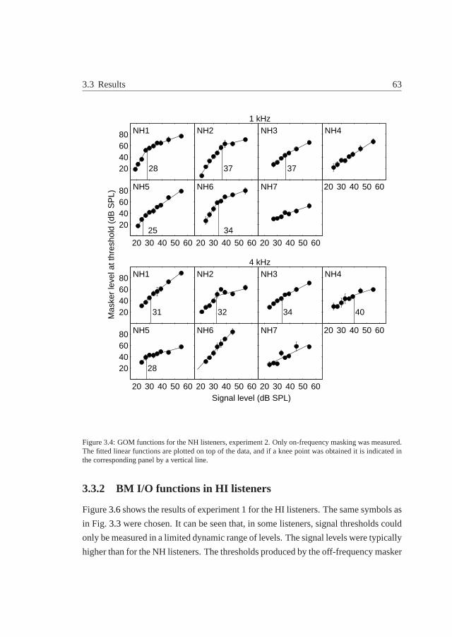
i

i

“MainFile” — 2010/7/15 — 15:31 — page 63 — #83i

i

i

i

i

i

3.3 Results 63

20406080 NH1

28

20406080 NH1

31Mas

ker

leve

l at t

hres

hold

(dB

SP

L)

NH2

37

1 kHz

NH2

32

4 kHz

NH3

37

NH3

34

20 30 40 50 60

NH4

20 30 40 50 60

NH4

40

20 30 40 50 60

20406080 NH5

25

20 30 40 50 60

20406080 NH5

28

20 30 40 50 60

NH6

34

20 30 40 50 60

NH6


20 30 40 50 60

NH7

20 30 40 50 60

NH7

Figure 3.4: GOM functions for the NH listeners, experiment 2.Only on-frequency masking was measured.The fitted linear functions are plotted on top of the data, andif a knee point was obtained it is indicated inthe corresponding panel by a vertical line.

3.3.2 BM I/O functions in HI listeners

Figure3.6shows the results of experiment 1 for the HI listeners. The same symbols as

in Fig. 3.3were chosen. It can be seen that, in some listeners, signal thresholds could

only be measured in a limited dynamic range of levels. The signal levels were typically

higher than for the NH listeners. The thresholds produced bythe off-frequency masker

i

i

“MainFile” — 2010/7/15 — 15:31 — page 64 — #84i

i

i

i

i

i


NH1 NH2 NH3 NH4 NH5 NH6 NH7 mean SDCompression, 1 kHz 0.44 0.34 0.63 0.42 0.62 0.47 0.51 0.48 0.09Knee point, 1 kHz 28 37 37 - 25 34 - 32 5.4Compression, 4 kHz 0.26 0.32 0.30 0.45 0.36 0.17 0.22 0.30 0.09Knee point, 4 kHz 31 32 34 40 28 - - 33 4.5

Table 3.1: Overview of the estimated BM I/O parameters for the NH listeners: BM compression in dB/dBand knee point in terms of the input level in dB. The means and standard deviations (SD) are also listed

20

40

60

80

100 NH1 NH2 NH3

20 40 60 80 100

NH4

0 20 40 60 80 100

20

40

60

80

100 NH5

Out

put (

dB)

20 40 60 80 100

NH6

Input level (dB SPL)20 40 60 80 100

NH7

1 kHz4 kHz

Figure 3.5: Estimated BM I/O functions for the NH listeners obtained from combining the data of the twoexperiments. I/O functions are plotted such that an input level at 100 dB SPL produces a correspondingoutput at 100 dB. The solid and dashed curves indicate I/O functions at 1 and 4 kHz, respectively. Thedashed-dotted curves indicate the slope of 1.0 (linear relation).

were generally above those found with the on-frequency masker. In several cases, the

slopes of the on- and off-frequency masking GOM functions were more similar than

found in the NH listeners. This is consistent with recent findings by, e.g.,Rosengard

et al. (2005). The estimated compression was calculated and is listed inTable3.2.

i

i

“MainFile” — 2010/7/15 — 15:31 — page 65 — #85i

i

i

i

i

i

3.3 Results 65

The compression ratios range from being close to normal (0.31 dB/dB) to about one

indicating linear BM processing.

40

60

80

100HI1

40

60

80

100

Mas

ker

leve

l at t

hres

hold

(dB

SP

L)

HI1

HI2

1 kHz

HI2

4 kHz

40 50 60 70 80 90

HI3

40 50 60 70 80 90

HI3

40 50 60 70 80 9040

60

80

100HI4

40 50 60 70 80 9040

60

80

100HI4

40 50 60 70 80 90

HI5

40 50 60 70 80 90Signal level (dB SPL)

HI5


Figure 3.6: Results of experiment 1, as in Fig.3.3, but for the five HI listeners.

Knee points were estimated from the data in Fig.3.7. Multi-phase regression

lines were calculated as described earlier, and the fitted linear curves are represented

by the solid curves. In four cases (e.g., HI2 and HI4 at 1 kHz),where the knee-

point estimates are in the normal range (39 to 45 dB), the results reflect the scenario in

i

i

“MainFile” — 2010/7/15 — 15:31 — page 66 — #86i

i

i

i

i

i


HI1 HI2 HI3 HI4 HI5Compression, 1 kHz 0.69 0.65 0.55 1.11 0.50Knee point, 1 kHz (70) 40 - 39 (50)Compression, 4 kHz 0.54 0.76 0.31 0.39 0.85Knee point, 4 kHz (59) - - 40 45

Table 3.2: As Table 3.1, but for the HI listeners. Knee pointsin brackets indicate particular cases, asdescribed in Fig 1, panels B1 and B2.

A1/A2 in Fig.3.1. In three other cases cases (HI1 and HI5 at 1 kHz; and HI1 at 4 kHz),

the results reflect the B1/B2 scenario, and in these cases theknee-point estimates are

at higher-than-normal levels (70, 50 and 59 dB, respectively). In the remaining three

cases, no reliable estimate of the knee point could be obtained. For the HI listeners,

there are several conditions where one of the two lines in theregression-line fits were

based on only few data-points.

As for the NH listeners, the estimates of the complete BM I/O functions were

derived from the results from the two experiments. Fig.3.8shows the individual I/O

functions for the five HI listeners.It is clear that these I/Ofunctions are very different

across the five listeners, and depend on frequency within each listener. When no

knee-point estimates were obtained, only the compressive part of the I/O function is

shown (e.g., HI3 at 1 kHz). Fig.3.9 shows estimated BM compression as a function

of pure-tone sensitivity (left panel) and the knee-point estimates as a function of

sensitivity (right panel). No significant correlation was observed in either case. The

correlation coefficients (ρ) for the data in the left and right panels were 0.0018 and

0.26, respectively.

i

i

“MainFile” — 2010/7/15 — 15:31 — page 67 — #87i

i

i

i

i

i

3.3 Results 67

20406080 HI1

70

20406080 HI1

59

Mas

ker

leve

l at t

hres

hold

(dB

SP

L)

HI2

40

1 kHz

HI24 kHz

30 40 50 60 70 80

HI3

30 40 50 60 70 80

HI3

30 40 50 60 70 80

20406080 HI4

39

30 40 50 60 70 80

20406080 HI4

40

30 40 50 60 70 80

HI5

50

30 40 50 60 70 80

HI5

45


Figure 3.7: Results of experiment 2, as in Fig.3.4, but for the five HI listeners.

i

i

“MainFile” — 2010/7/15 — 15:31 — page 68 — #88i

i

i

i

i

i


20

40

60

80

100 HI1 HI2

20 40 60 80 100

HI3

0 20 40 60 80 100

20

40

60

80

100 HI4

Out

put l

evel

(dB

)

20 40 60 80 100

HI5


1 kHz4 kHz

Figure 3.8: As in Fig. 3.5, but for the five HI listeners.

0 10 20 30 40 500.2

0.4

0.6

0.8

1

1.2

Pure−tone threshold (dB HL)

BM

com

pr. (

dB/d

B)

1 kHz4 kHz

0 10 20 30 40 5030

40

50

60

70

80


Kne

e po

int (

dB)

1 kHz4 kHz

Figure 3.9: Scatter-plots of the relations between the pure-tone thresholds (sensitivity) and estimatedcompression (left panel) and knee points (right panel)

i

i

“MainFile” — 2010/7/15 — 15:31 — page 69 — #89i

i

i

i

i

i

3.4 Discussion 69

3.4 Discussion

The measured thresholds in both experiment 1 and 2 showed lowwithin-listener

variability. This was earlier emphasized as being one of themajor advantages

of the GOM method over the TMC method (Rosengardet al., 2005). Estimates

of compression were found to be similar across NH listeners,with estimated

compression exponents at 1 kHz being slightly higher than at4 kHz. This is

consistent with the observation inMooreet al. (1999); Rosengardet al. (2005). The

estimated compression in the HI listeners varied substantially, as expected from earlier

investigations. No correlation between the loss of sensitivity and the estimated amount

of compression was found (ρ = 0.0018). Mooreet al. (1999) collected data in six HI

listeners with moderate to severe hearing loss. They found aslight correlation between

sensitivity and compression estimates for cases where the loss was larger than 35 dB.

The listeners from the present study typically had losses less than 35 dB at the tested

frequencies which might be the reason for why no correlationwas found.

The main contribution of this study was that estimates of both compression

exponents and knee point levels were obtained. This was achieved by adding an

extra forward masking condition with a longer masker-signal interval. This allows

characterization of the BM I/O function for a wider range of input levels. Presently,

this is the first behavioral study that use an experimental condition designed to

explicitly determine the BM I/O function knee point. It was shown that this can

be done reliably. For all NH listeners, except NH7, clear significant knee-point

estimates could be obtained. An advantage was that the only change from experiment

2 to experiment 1 was the changed MSI. Thus, the additional experiment requires

additional testing time, but no further training. The experiment was sensitive to the

choice of the MSI, since the number of measured thresholds above and below the

knee-point need to be sufficient. However, it seems the the MSI chosen here (12 ms)

was appropriate for all NH listeners. For the HI listeners, knee points were obtained

in 7 of the 10 I/O-functions estimates. Some of these estimates relied on few data-

points. This could be avoided by choosing the MSI of experiment 2 to be listener

specific, based on a pilot run testing a range of MSIs. If the MSI is too short, the

levels of the masker and the signal are too similar, and both stimuli are processed

i

i

“MainFile” — 2010/7/15 — 15:31 — page 70 — #90i

i

i

i

i

i


in the same, either linear or compressive, region, such thatno transition point could

be identified. This could be the reason why no knee points could be found for HI3

(at both frequencies) and HI2 (at 4 kHz). If the MSI is too long, the level of the

masker approaches the maximally allowed presentation level of 100 dB SPL, which in

turn, reduced the dynamic range of tested input levels in thedata reflecting condition

A1. Three of the estimated I/O functions showed support of the idea that the knee

point is shifted towards higher levels (Placket al., 2004). However, only one of these

(HI5 at 1 kHz) approached a near-normal compression exponent. Four other I/O-

function estimates showed a trend where the knee point was close to normal while

less compression was found. It was also tested whether therewas a relation between

the HI listener sensitivity and corresponding estimated knee points. No significant

correlation was found (ρ = 0.26).

Recently,Wojtczak and Oxenham(2009) discussed that the assumption underly-

ing the GOM method may not be appropriate, since on- and off-frequency maskers

show a different recovery from masking at a particular placeon the BM, even when

the amount of excitation was adjusted to be the same at that place. This means that the

amount of compression may be overestimated (lower compression exponents) using

forward masking methods to estimate BM compression.Wojtczak and Oxenham

(2009) concluded that results obtained with the GOM method are less likely to

overestimate compression compared to the TMC method. The mean estimates of

compression for the NH listeners of the present study were 0.48 at 1 kHz and 0.30

at 4 kHz. This was slightly higher than, although consistentwith, results from other

studies (e.g.,Rosengardet al., 2005). The results ofPlacket al. (2004) were obtained

with the TMC method, and they found near-normal compressionabove the knee point.

This was only observed in 2 out of 10 conditions in the HI listeners from the present

study. For the remaining conditions the compression exponents were higher. The

disadvantage of using the GOM method over the TMC method is the requirement of

ipsi-lateral masking noise to avoid off-frequency listening, and contra-lateral masking

noise to prevent across ear listening. It is not clear how to choose the levels of these

noises appropriately for HI listeners. Here, these masker noise levels were chosen

relatively lower than those used for NH listeners. The HI listeners may not have

the off-frequency cues available due to their reduced sensitivity, and furthermore, the

i

i

“MainFile” — 2010/7/15 — 15:31 — page 71 — #91i

i

i

i

i

i

3.4 Discussion 71

noise masker levels used for the NH listeners were too high, such that they would

be distractive to the HI listeners. The finding of large individual differences in BM

I/O functions motivate the importance of characterizing hearing loss on an individual

basis, e.g. in terms of BM compression and BM tuning in addition to the audiogram.

The valuable contribution from the present study is that thesuggested experiment

provides reliable estimates of the I/O-function knee point, which is an important

parameters when nonlinear I/O-functions of the BM stage in amodel is fitted to

individual hearing loss. Such model allows to investigate the underlying mechanisms

of cochlear hearing loss. This was investigated inJepsen and Dau(2010) (chapter4

of this thesis).

i

i

“MainFile” — 2010/7/15 — 15:31 — page 72 — #92i

i

i

i

i

i


3.5 Conclusions

• In experiment 1, forward masking using on- and off-frequency was measured,

and the results were used to obtain an estimate of basilar-membrane compres-

sion. In experiment 2 a different forward masking conditionwas used and the

results were used to obtain estimates of the knee point of thebasilar-membrane

input-output function. By combining the results of experiment 1 and 2 an

estimate in the complete BM I/O function was obtained in seven normal-hearing

and five hearing impaired listeners.

• The method extends the input level range in which I/O functions can be

estimated compared to other forward masking paradigms. However, the

suggested method requires additional testing time.

• For the NH listeners the choice of masker-signal intervals in experiment 2 was

constant and provided reasonable knee-point estimates. However, for the HI

listeners an individual-specific choice of masker-signal interval is necessary to

obtain reliable knee-point estimates.

i

i

“MainFile” — 2010/7/15 — 15:31 — page 73 — #93i

i

i

i

i

i

3.6 Appendix: Additional information about the listeners 73

3.6 Appendix: Additional information about the lis-

teners

This appendix describes additional information about the hearing-impaired listeners

that were used in Chapter 3 and is listed in Table3.3. The etiologies of the hearing

losses are listed, and they are based on clinical diagnoses if available. It is also listed

whether the listeners were hearing-aid users or not. Finally, results from a speech

intelligibility test are listed. These results were not used or analyzed in the chapter,

but are reported here to make these data available to possible future studies.

Speech reception thresholds (SRTs) were measured for Danish Dantale II

sentences in two noise conditions. It is a closed-set word recognition test using

Hagerman sentences (Wageneret al., 2003). The noise conditions were: (1) stationary

speech-shaped noise (SSN) with the long-term spectrum of the Dantale II sentences;

(2) sinusoidally amplitude modulated (SAM) noise with a constant modulation rate

at 8 Hz and a modulation depths of 1. The SRT was defined as the SNR at which

50% words were identified correctly. The noise level was constant wihle the level of

the sentences was varied adaptively. Listeners were trained on a single run with 20

sentences before measurements were made. The reported SRTsare avereages of two

measurements. The mean SRT results of the seven NH listenersare also given in the

table.

Listener Etiology Hearing-aid user SSN SAMHI1 Presbycusis No -2.6 -4.8HI2 Noise induced Yes -5.6 -6.3HI3 Presbycusis Yes -6.6 -8.7HI4 Unknown No -6.5 -9.2HI5 Presbycusis Yes -7.1 -8.5Mean NH -7.6 -16.7

Table 3.3: Additional information about the five HI listenersused in Chapter 3. The table lists their hearingloss etiology, hearing aid use and SRTs (in dB) in noise condition of stationary speech-shaped noise (SSN)and Sinusoidally amplitude modulated (SAM) noise at a modulation rate of 8 Hz.

i

i

“MainFile” — 2010/7/15 — 15:31 — page 74 — #94i

i

i

i

i

i


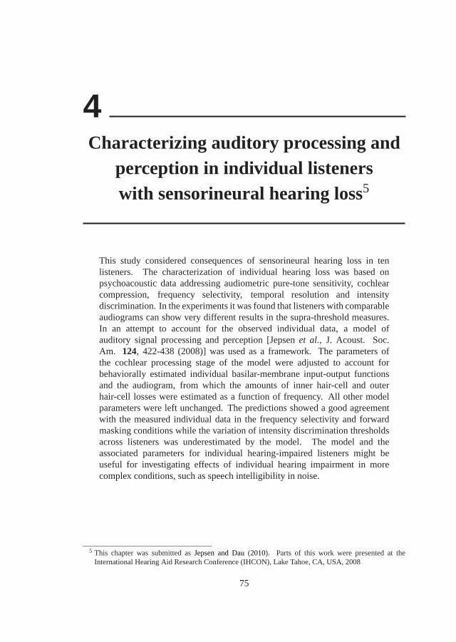
i

i

“MainFile” — 2010/7/15 — 15:31 — page 75 — #95i

i

i

i

i

i

4Characterizing auditory processing and

perception in individual listenerswith sensorineural hearing loss5

This study considered consequences of sensorineural hearing loss in tenlisteners. The characterization of individual hearing loss was based onpsychoacoustic data addressing audiometric pure-tone sensitivity, cochlearcompression, frequency selectivity, temporal resolutionand intensitydiscrimination. In the experiments it was found that listeners with comparableaudiograms can show very different results in the supra-threshold measures.In an attempt to account for the observed individual data, a model ofauditory signal processing and perception [Jepsenet al., J. Acoust. Soc.Am. 124, 422-438 (2008)] was used as a framework. The parameters ofthe cochlear processing stage of the model were adjusted to account forbehaviorally estimated individual basilar-membrane input-output functionsand the audiogram, from which the amounts of inner hair-celland outerhair-cell losses were estimated as a function of frequency.All other modelparameters were left unchanged. The predictions showed a good agreementwith the measured individual data in the frequency selectivity and forwardmasking conditions while the variation of intensity discrimination thresholdsacross listeners was underestimated by the model. The modeland theassociated parameters for individual hearing-impaired listeners might beuseful for investigating effects of individual hearing impairment in morecomplex conditions, such as speech intelligibility in noise.

5 This chapter was submitted asJepsen and Dau(2010). Parts of this work were presented at theInternational Hearing Aid Research Conference (IHCON), Lake Tahoe, CA, USA, 2008

75

i

i

“MainFile” — 2010/7/15 — 15:31 — page 76 — #96i

i

i

i

i

i

76 4. Characterizing auditory processing in hearing impairment

4.1 Introduction

Hearing impairment is a communicative handicap: hearing-impaired (HI) people often

experience great difficulty with speech communication. These difficulties are typically

most pronounced when background noise is present, in reverberant environments or in

situations with multiple interfering sound sources. The most common form of hearing

loss can be attributed to damage to the inner ear, or cochlea,where the most obvious

symptom is a loss of ability to detect weak sounds. This is accompanied by a variety

of other changes in the way that sound is perceived. Even if sounds are amplified

by a hearing aid such that reduced audibility is compensatedfor, many listeners still

experience problems in every-day life situations. There can be enormous differences

in performance between individual listeners to whom a hearing aid has been fitted

(Lunner, 2003). Some listeners might be satisfied with their aids while others continue

to experience difficulties when listening to speech in noiseor competing speech. In

order to choose the right compensation strategy for the individual hearing-impaired

listener, one needs to understand where the sources of this variability among the

listeners are. It is important to clarify what the limitations besides audibility are and

how they can be characterized. Furthermore, if the performance of individual listeners

could be predicted through auditory modeling, this would beparticularly useful to help

design the best compensation strategy for the individuals.

The present study had two major goals. One goal was to experimentally

characterize individual hearing impairment, using a set ofmeasures of auditory

function. The second goal was to quantitatively account forindividual hearing

impairment using a model of auditory signal processing and perception. The

study focused on perceptual consequences of sensorineuralhearing loss (SNHL).

Typical consequences of this type of hearing loss are reduced sensitivity, loudness

recruitment, reduced temporal resolution and reduced frequency selectivity (e.g.,

Moore, 1995). While reduced sensitivity explains part of the communication

difficulties in HI listeners, some of the reported variability in performance among

listeners may be due to supra-threshold deficits. Loudness recruitment as well

as reduced frequency selectivity and reduced temporal resolution are examples of

"supra-threshold" consequences. In the present study, basic functions of auditory

i

i

“MainFile” — 2010/7/15 — 15:31 — page 77 — #97i

i

i

i

i

i

4.1 Introduction 77

processing in HI listeners were investigated, using psychoacoustic masking and

discrimination experiments. These measures included the sensitivity to pure tones

in terms of the audiogram; temporal masking curves (TMC;Nelsonet al., 2001)

to estimate individual basilar-membrane (BM) input-output (I/O) functions; notched-

noise masking to estimate individual auditory filter bandwidths (Patterson and Moore,

1986); simultaneous and forward masking with noise maskers (Glasberget al.,

1987) to estimate temporal resolution; and intensity discrimination for tones to

estimate intensity resolution. This approach was similar in Moore et al. (1999)

where measures of sensitivity and frequency selectivity and their relations to hair-

cell loss and changes in BM compression were investigated. However, in contrast

to Mooreet al. (1999) who focused on correlations between measures, the goal here

was to characterize individual hearing impairment using a "critical" set of outcome

measures. Furthermore, several conditions of non-simultaneous and simultaneous

masking were considered which were not studied inMooreet al. (1999). The results

of the experiments served as the basis for the subsequent modeling efforts described

further below.

In the normally functioning system, the BM I/O function has an approximately

linear region at low input sound pressure levels (< 30-40 dB)and a compressive

region at medium and high sound pressure levels (< 90 dB) (Ruggeroet al., 1997).

The transition point between the linear and the compressiveregion reflects the knee

point. Some studies observed a return to linear processing for levels above about

90 dB SPL (e.g.,Nelsonet al., 2001). Several studies have suggested methods to

behaviorally estimate the BM I/O function and, thus, the amount of BM compression

in humans (e.g.,Oxenham and Plack, 1997; Nelsonet al., 2001). Nelsonet al. used

forward masking with pure-tone signals and maskers and measured TMCs where the

signal level was fixed and the temporal separation between the masker and the signal

varied. Based on this, an estimate of the shape of the BM I/O function was obtained,

including estimates of the amount of compression and the knee point. This method

has since been used in several studies with normal-hearing and hearing-impaired

listeners (Nelsonet al., 2001; Lopez-Povedaet al., 2003, 2005; Placket al., 2004;

Stainsby and Moore, 2006). In these studies, a reduced or loss of compression was

found in HI listeners with severe loss, resulting in a linearor close to linear I/O

i

i

“MainFile” — 2010/7/15 — 15:31 — page 78 — #98i

i

i

i

i

i


function (Nelsonet al., 2001; Stainsby and Moore, 2006) which is in line with the

assumed effect of a loss of OHCs in such listeners. Other studies dealt with mild-to-

moderate losses (Placket al., 2004; Lopez-Povedaet al., 2005; Dubnoet al., 2007;

Jepsen and Dau, 2008) where it was found that the estimated I/O functions strongly

depended on the individual listener. Some listeners showedan increased compression

exponent, i.e. less compression, while others also indicated a shift in the knee point

between the linear and compressive region.

In a SNHL, the number of hair cells in the cochlea is typicallyreduced due to age,

hereditary disease, noise trauma or exposure to drugs from medical treatment (e.g.,

Moore, 2007). The hair cells are divided into outer hair cells (OHCs) andinner

hair cells (IHCs). The OHCs are commonly associated with nonlinear gain in the

cochlea (e.g.,Ruggeroet al., 1997). At low stimulation levels, the OHCs amplify the

basilar-membrane (BM) response. The amount of gain provided by the OHCs is level

dependent; with increasing input level, the OHC gain decreases. This is equivalent

to the BM input-output (I/O) function being non-linear and compressive. It is an

important property of the normally-functioning inner ear that a wide dynamic range

of input levels is transformed into a narrower dynamic rangeat its output. The OHCs

are also responsible for the sharp tuning of the BM at low stimulation levels, a feature

which is important for the ability to spectrally resolve complex sounds. The IHCs are

responsible for the transduction of the BM motion into electrical potentials that are

further processed by the subsequent neural system along theauditory pathway (e.g.,

Pickles, 2008). In listeners with SNHL, just noticeable differences (JNDs) in

intensity are typically similar as or higher than in NH listeners when the stimuli are

presented at the same SL, whereby thresholds can vary considerably among individual

listeners (Florentineet al., 1993).

It is still unclear how the loss of OHCs and IHCs can be estimated. showed that

The degree of OHC- and IHC loss has been shown to strongly depend on the individual

listener or animal preparation (e.g.,Liberman and Dodds, 1984; Mooreet al., 1999;

Heinz and Young, 2004). The variability may arise from differences in the cause of

the loss, e.g., due to differences in the intensity and duration of noise exposure (Borg

and Engström, 1989). Important effects are reduced OHC gain and, in consequence,

reduced BM compression and frequency selectivity. Loss of IHCs primarily has an

i

i

“MainFile” — 2010/7/15 — 15:31 — page 79 — #99i

i

i

i

i

i

4.1 Introduction 79

influence on sensitivity. It has also been hypothesized thatIHC loss may affect the

temporal acuity of the neural coding, or phase locking (e.g., Moore, 2007); however,

clear physiological evidence has not been provided yet (e.g., Heinz et al., 2002).

IHC loss has been observed to affect the temporal acuity of the neural coding, or

phase locking, but this is not necessarily always the case (see e.g.,Moore, 2007).

These aspects of a cochlear hearing loss cannot be characterized or predicted from the

audiogram alone. Estimates of the degree of impairments andthe relation between

OHC- and IHC loss in the impaired listeners would be important for characterizing

consequences of individual impairment.Moore et al. (1999) observed a reduced

sensitivity to pure tones in their HI listeners, referred tohere as "total hearing loss"

(HLTOT). They further used a loudness matching experiment to obtain an estimate of

the contribution of OHC loss to the reduced audibility (HLOHC). They estimated IHC

loss (HLIHC) from HLTOT and HLOHC, assuming that HLTOT = HLOHC+HLIHC. Heinz

and Young(2004) measured the growth of auditory-nerve responses as a function

of level in cats after acoustic trauma. They observed different impaired response

functions, some of which were primarily based on OHC loss, some were primarily

resulting from IHC loss and others were based on a more equal distribution of OHC

and IHC losses. The observations from these studies demonstrated the importance of

characterizing individual SNHL.

To address the second main goal of this study, which was to simulate individual

hearing impairment, the computational auditory signal processing and perception

(CASP) model ofJepsenet al.(2008) was used as a framework. The model consists of

various processing stages including, outer- and middle-ear filtering, nonlinear cochlear

processing, effects of adaptation, a modulation filterbankand an optimal detector

as the decision stage. This model which is based on the original model ofDau et

al. (1997a) but includes a nonlinear cochlea stage instead of the linear gammatone

filterbank, was shown to account for a large variety of detection and masking data in

normal-hearing listeners (Jepsenet al., 2008). In the present study, modifications of

the model were undertaken in the cochlear stage of the model.These modifications

were exclusively based on the individual estimates of the BMI/O functions derived

from the TMC data and the audiogram from this study. Even though the model

contains numerous parameters in the different processing stages, only very few (five)

i

i

“MainFile” — 2010/7/15 — 15:31 — page 80 — #100i

i

i

i

i

i


frequency-dependent parameters were considered for modification to account for the

individual losses. The model was used to predict the measured thresholds obtained in

the NH and individual HI listeners. Some of the parameters ofthe cochlear stage

of the model were adjusted to fit estimates of BM compression derived from the

psychophysical data, and measured loss of sensitivity. This approach has the principal

limitation that such behavioral estimates are themselves based on assumptions and

concepts which might not be fully justified and valid.

The CASP model represents only one example of an auditory processing model.

In fact, explaining basic auditory masking phenomena in terms of physiological

mechanisms has a long tradition. There have been systematicattempts at predicting

psychophysical performance limits (both in the NH and HI system) from the activity

of auditory nerve (AN) fibers (e.g.,Siebert, 1965, 1970; Heinz et al., 2001a,b,c;

Colburnet al., 2003; Bruceet al., 2003; Zilany and Bruce, 2006, 2007), combining

analytical and computational population models of the AN with statistical decision

theory. Different approaches to simulate effects of SNHL have been suggested (e.g.,

Kates, 1991; Bruce et al., 2003; Zilany and Bruce, 2006). A general result has

been that those models that make optimal use of all availableinformation from the

AN (e.g., average rate, synchrony, and nonlinear phase information) typically predict

performance that is one to two orders of magnitude better than human performance,

while the trends often match well human performance (e.g.,Heinz et al., 2001a).

Other types of auditory models are to a lesser extent inspired by neurophysiological

findings and make simplifying assumptions about the auditory processing stages. Such

an "effective" modeling strategy does not allow conclusions about the details of signal

processing at the neuronal level; on the other hand, if the model accounts for a variety

of data, this suggests certain processing principles. For example, the temporal window

model (e.g.,Oxenham and Moore, 1994; Oxenhamet al., 1997; Plack and Oxenham,

1998; Plack et al., 2002) has been shown to account for forward and backward

masking data in NH and sensorineural HI listeners as well as for other phenomena

associated with temporal resolution such as gap detection.The temporal window

model includes an initial stage of bandpass filtering (reflecting a simplified action of

BM filtering), followed by a nonlinear device, a smoothing device (implemented as a

lowpass filter or a sliding temporal integrator) and finally adecision device. The CASP

i

i

“MainFile” — 2010/7/15 — 15:31 — page 81 — #101i

i

i

i

i

i

4.1 Introduction 81

model, chosen here, lies conceptually between the two approaches described above. It

reflects a perception model designed to account for perceptual data, as the temporal-

window model, and is thus less accurate than the AN models in terms of details of

peripheral processing. However, it makes several additional assumptions about the

processing at and subsequent to the cochlear stage, such as effects of adaptation,

modulation filterbank and template-based optimal detection. Since this framework

has led to successful predictions of a large variety of perceptual masking data in NH

listeners it was chosen here to consider consequences of cochlear hearing impairment.

i

i

“MainFile” — 2010/7/15 — 15:31 — page 82 — #102i

i

i

i

i

i


4.2 Auditory processing model

The structure of the CASP model (Jepsenet al., 2008) is shown in Fig.4.1. The

processing stages comprise outer- and middle-ear filters, nonlinear BM processing,

inner hair-cell transduction, expansion, adaptation and amodulation filterbank.

Finally, the model includes an optimal detector designed todeal with n-interval

alternative forced choice paradigms.

+

DRNL filterbank

Lineargain

Gammatonefilter

Lowpassfilter

Broken sticknon-linearity


Expansion

Adaptation

Outer- and middle-ear TF

+

Optimal detector

Modulation filterbank

Gammatonefilter

Gammatonefilter

Lowpassfilter

Internal noise

Figure 4.1: Schematic structure of the CASP model. The model comprises: outer- and middle ear filtering,the DRNL filterbank, inner hair-cell transduction, expansion, adaptation, a modulation filterbank and anoptimal detector. The gray blocks indicate the stages in which adjustments are made to fit individualhearing loss. In the DRNL filterbank, the gain in the linear path and parameters controlling the broken-stick nonlinearity are fitted. IHC loss is implemented in the IHC transduction stage.

i

i

“MainFile” — 2010/7/15 — 15:31 — page 83 — #103i

i

i

i

i

i

4.2 Auditory processing model 83

4.2.1 Stages of the auditory processing

The first stage is an outer- and middle-ear stage implementedas two finite impulse

response filters as inLopez-Poveda and Meddis(2001). The second stage is the dual-

resonance nonlinear (DRNL) filterbank as inLopez-Poveda and Meddis(2001). The

model uses parallel processing in two independent paths. The linear path comprises

linear gain,g, a cascade of gammatone filters and a subsequent lowpass filter, and can

be regarded as describing the “passive” BM response. The nonlinear path comprises

cascaded gammatone filters, a broken stick nonlinearity (Eq. 4.1), another cascade of

gammatone filters and a lowpass filter and can be associated with the “active” part of

the BM response. The summed signal of the two paths describesthe nonlinear BM

processing and accounts for level-dependent compression and tuning. The broken-

stick nonlinearity is defined as follows:

y[i] = sign(x[i]) · min(a|x[i]|, b|x[i]|c) (4.1)

wherebyy represents the output signal andx is the input signal,i refers to theith

sample anda, b andc are parameters. After this stage, the signal analysis is performed

separately in different frequency channels.

Inner hair-cell transduction is modeled as a half-wave rectification followed by a

first-order lowpass filter with a cut-off frequency at 1 kHz. Effectively, it preserves

phase information (fine-structure) at low frequencies while the signal envelope is

extracted at higher frequencies. The expansion stage transforms the output of the

IHC stage into an intensity-like representation by applying a squaring expansion.

Effects of adaptation are simulated by a chain of five simple nonlinear circuits, or

feedback loops, which include different time constants in the individual loops (Dau

et al., 1996a). For stationary input signals, the output of the series of five loops

approaches a logarithmic compression. For input variations that are rapid compared to

the time constants (τ ) of the lowpass filters (withτ in the range from 5 to 500 ms), the

transformation through the adaptation loops is more linear, leading to an enhancement

of fast temporal variations at the output of the adaptation stage. For example, in

response to signal onsets, the output of the adaptation loops is characterized by a

pronounced overshoot. In order to simulate absolute threshold, the lower limit of the

i

i

“MainFile” — 2010/7/15 — 15:31 — page 84 — #104i

i

i

i

i

i


input to the adaptation loops, and thus the size of the dynamic range in the model,

was chosen here to be different for different frequency channels such that the model

for normal hearing predicts the 0 dB hearing level (HL) line in the simulation of the

audiogram (see gray squares in the top left panel in Fig.4.3). This lower limit used

to be frequency independent inDauet al. (1996a, 1997a,b) andJepsenet al. (2008)

where the focus was on signal in noise detection while pure-tone sensitivity in quiet

was not considered in detail.

The output of the adaptation stage is processed by a first-order lowpass filter

with a cut-off frequency at 150 Hz. The lowpass filter is followed by the

modulation filterbank which is a bank of bandpass filters tuned to different modulation

frequencies. The decision device is realized as an optimal detector. It derives a

template of the model’s internal representation, using a supra-threshold representation

of the signal in the target interval, and a representation ofthe reference intervals

(Dauet al., 1996a,b). The internal representation of the stimuli after the modulation

filterbank is a three-dimensional pattern with axes time, center frequency and

modulation frequency. In the present study, the templates were derived from the

model fitted to the individual listener; thus, the templatesused to simulate the effects

of hearing impairment were based on the impaired, i.e. the not normal, auditory

processing. Internal noise is added to the internal representation in order to limit

the model’s resolution and match human performance. The variance of this noise was

adjusted such that the model follows Weber’s law in intensity discrimination with

pure tones, at a reference level of 60 dB SPL (Dau et al., 1996a). The variance

was kept constant in all simulations. It was determined in the model of normal

hearing and assumed to be the same in listeners with SNHL. Theeffect of the internal

noise depends on the experimental conditions. For example,if a masking experiment

is simulated and stochastic maskers are used, then theexternal variability of the

stimuli typically dominates, whereas performance is limited by the internal noise in

experiments using deterministic maskers. For further details, the reader is referred

to Dauet al. (1996a, 1997a,b) andJepsenet al. (2008).

i

i

“MainFile” — 2010/7/15 — 15:31 — page 85 — #105i

i

i

i

i

i


4.2.2 Parameter changes to account for SNHL

To simulate consequences of sensorineural hearing loss, the stages associated with

hair-cell loss were modified. The changes were thus includedin the DRNL filterbank

and the IHC transduction stage. The input-output behavior of the DRNL filter is

determined by the interaction of the linear and the nonlinear path. The resulting knee

point and compression exponent are therefore not solely defined by the broken-stick

nonlinearity. The linear path has more dominance when the linear gain,g, is increased,

leading to a linear response at high input levels. Parameters a andb in the broken-

stick nonlinearity (Eq.4.1) can be adjusted to fit the target knee point. The relation

between the values ofa andb determines the level at which the transition from linear to

compressive processing (the knee point) occurs. By decreasing a, the low-level linear

part will be extended, thus shifting the knee point towards higher levels. A decrease

of b extends the compressive region towards lower levels, thus shifting the knee point

towards lower levels. Parameterc is the compression exponent and will resemble the

effective compression of the complete input-output function where the termb|x[i]|cin Eq. 4.1 is smallest. The interaction betweena, b, c andg determines the resulting

compression exponent of the complete DRNL I/O function.

In the present study, these four parameters were adjusted tofit the BM I/O

functions of the individual listeners. This was done manually. The first step was to

adjust a and b in parallel according to the estimated knee, orto the lowest measurable

point in the TMC data. The DRNL I/O function was assumed to be linear for levels

below this level or the knee point. It was further assumed that the compression

exponent (parameterc) of the fitted DRNL I/O functions cannot be below that of the

DRNL I/O functions simulating normal hearing. Parameterc was only in few cases

adjusted, since the adjusteda andb already influenced the effective compression in

the compressive region. Finally, parameterg was adjusted such that the extent of

the compressive region was matching the estimated I/O function. The DRNL I/O

function was assumed to be linear for levels below the lowestmeasurable point in

the TMC data. It was further assumed that the compression exponent (parameterc)

of the fitted DRNL I/O functions cannot be below that of the DRNL I/O functions

simulating normal hearing. The parameters were determinedat 1 and 4 kHz. For

other filter center frequencies (from 0.05 to 10 kHz in 25 Hz steps), the corresponding

i

i

“MainFile” — 2010/7/15 — 15:31 — page 86 — #106i

i

i

i

i

i


parameters were obtained using a linear interpolation and extrapolation procedure.

This procedure was the same as the one used in the regression analysis inLopez-

Poveda and Meddis(2001) to derive the DRNL parameters at arbitrary filterbank

frequencies. Linear interpolation was performed such thatthe parameters followed

the form log10

(parameter)= p0 + m · log10

(BF ), wherep0 and m describe the

offset and slope of the linear relation, respectively, andBF denotes the filter’s center

frequency in Hz.

An estimate of OHC loss in terms of sensitivity loss was obtained from the fitted

DRNL I/O function. It was assumed that the output magnitude of the "normal" DRNL

I/O function for an input level of 0 dB SPL reflects absolute sensitivity of this stage.

Figure4.2shows the I/O functions of the DRNL model for normal hearing at different

frequencies. The filters centered at 250 (open squares) and 500 Hz (open circles)

have their knee points shifted towards at higher input levels and their low-level linear

parts are extended compared to the functions shown for the higher frequencies. One

consequence is that the maximum amount of OHC loss that can besimulated is lower

than at higher center frequencies, since the I/O functions for these low-frequency

filters reflect less nonlinear gain. Similar frequency-dependent knee points were

observed in the pulsation threshold data ofPlack and Oxenham(2000), to which the

original version of the human DRNL filterbank was fitted (Lopez-Poveda and Meddis,

2001). The previoulsy proposed animal filterbank (Meddiset al., 2001) also simulated

limited compression at low center frequencies based on dataof Rhode and Cooper

(1996). It is now commonly assumed that on-frequency BM compression is frequency

independent (Lopez-Povedaet al., 2003). However, a modification of the DRNL to

comply with these findings has been outside the scope of the present study. Table4.1

shows the frequency-dependent maximum amount of OHC loss aspredicted by the

DRNL model.

The amount of IHC loss (HLIHC) was estimated as the difference between HLTOT

(as measured in the audiogram) and HLOHC (estimated from the fitted DRNL I/O

functions). Liberman and Dodds(1984) found that noise-induced damage to the

IHCs, mainly causes elevated tuning curves. Here, it was assumed that HLIHC can be

simulated as a linear attenuation at the output of the hair-cell transduction stage. Other

studies involving simulation of IHC loss use similar and simple forms of attenuation,

i

i

“MainFile” — 2010/7/15 — 15:31 — page 87 — #107i

i

i

i

i

i


0 20 40 60 80 100

0

10

20

30

40

50

60

70

80

90

100


DR

NL

outp

ut (

dB)

250 Hz500 Hz1 kHz2 kHz4 kHz8 kHz

Figure 4.2: DRNL input-output functions at different center frequencies ranging from 0.25 to 8 kHz. Thefunctions are aligned such that an input level of 100 dB SPL produces a model output of 100 dB. The dottedline indicates linear processing.

Center frequency (kHz) 0.25 0.5 1 2 4 8Max HLOHC (dB) 17 25 34 38 43 45Knee point (dB) 65 45 30 20 30 40Compression (dB/dB) 0.35 0.35 0.25 0.25 0.25 0.25

Table 4.1: Maximum HLOHC that can be simulated by the DRNL filterbank at different center frequenciesas well as the values for the simulated knee point and compression of the DRNL simulating normal hearing.

although implemented in different ways (e.g.,Kates, 1991; Bruceet al., 2003; Zilany

and Bruce, 2006). It was assumed that HLIHC can be simulated as a linear attenuation

at the output of the hair-cell transduction stage. Linear interpolation was used to

obtain attenuation factors for frequencies from 0.05 to 10 kHz with a resolution of 25

Hz. This was done for each individual listener.

i

i

“MainFile” — 2010/7/15 — 15:31 — page 88 — #108i

i

i

i

i

i


4.3 Experimental method

4.3.1 Test subjects

Ten hearing-impaired (HI) and three normal-hearing (NH) listeners participated in

this study. All HI listeners had a SNHL indicated by air-bonegaps of less than

10 dB in their pure-tone audiograms. Only one ear of each subject was measured.

The measured audiograms of all ten listeners are shown in Fig. 4.3 and indicated

as open symbols. Additional information, e.g., listener’sage and gender, can be

found in Table4.2 and in Sec.4.7. The filled symbols indicate simulated thresholds

which will be described in section4.4.2. The listeners consisted of six males and

four females, aged between 48 and 73 years. Seven of the ten listeners were using

hearing aids regularly. The measurements in this study werecarried out without

hearing-aid amplification. Two of the HI listeners had previous experience in listening

experiments. The three NH listeners (two males and one female, aged between 20 and

27 years) were included as a control group. All had audiometric pure-tone thresholds

below 10 dB HL. One of the NH listeners was the first author who had experience in

listening tests. All listeners (except the first author) were paid for their participation.

Measurement sessions were between 30 to 45 minutes long depending on the listener’s

self-reported ability to focus on the task. No appointment lasted for longer than two

hours. The amount of training depended on the experiment. Training was performed

until no systematic improvements in thresholds were observed. The TMC experiment

was the most demanding task and required two to four hours of training to reach stable

results. In all measurements except the audiogram, the subjects completed at least

three runs per condition. The total testing time for each subject, including training,

was 14 to 20 hours.


The pure-tone audiograms were measured manually with a PC-based clinical setting,

using the Interacoustics Affinity and Sennheiser HDA200 headphones. The same sys-

tem was used to perform the bone-conduction measurements. All other measurements

were carried out in a double-walled sound insulated booth with a computer monitor

i

i

“MainFile” — 2010/7/15 — 15:31 — page 89 — #109i

i

i

i

i

i


to provide instructions and visual feedback. The computer keyboard was used to

obtain the responses. The stimuli were presented monaurally via Sennheiser HD580

headphones. They were generated in MATLAB on a personal computer and converted

to analogue signals by a 24-bit soundcard (RME DIGI 96/8). The notched-noise

masking stimuli were generated at a sampling rate of 48 kHz. In the other experiments,

the sampling rate was at 44.1 kHz. FIR equalization filters were applied to obtain a flat

frequency response at the headphone output. A three-interval three-alternative forced

choice paradigm combined with a 1-up-2-down tracking rule was used, except for the

TMC experiment where a 2-up-1-down rule was applied. The reported thresholds thus

reflect the 70.7% point on the psychometric function and represent the mean of at least

three measurements. The step size was varied adaptively andthresholds represent an

average of the levels at the last eight reversals at the final step size. The listeners

received immediate feedback on whether a response was correct or not.

4.3.3 Stimuli

Temporal masking curves (TMC)

In the TMC experiment, forward masking of a fixed-level brieftone was measured

as a function of the signal-masker interval. The probe signal was a pure tone with

a duration of 20 ms, which was Hanning windowed over its entire duration. The

frequency (fsig) was either 1 or 4 kHz. The signal was presented at 10 dB sensation

level (SL). The masker was also a pure tone with a duration of 200 ms and 5-ms raised-

cosine on- and off ramps were applied. The masker frequency (fm) was equal tofsig

(on-frequency condition) or0.6 · fsig (off-frequency condition). The masker-signal

interval was 2, 5, 10 ms and additional 10-ms increments until the subject reported (in

pilot runs) that the masker level became uncomfortably loud, or reached the maximum

level of 102 dB SPL. The masker level was adjusted to reach masked signal threshold.

The initial step size was 8 dB and the final step size was 1 dB.

Notched-noise masking

In order to estimate the shape and bandwidth of the auditory filters, the notched-noise

masking method was used (Patterson and Nimmo-Smith, 1980; Patterson and Moore,

i

i

“MainFile” — 2010/7/15 — 15:31 — page 90 — #110i

i

i

i

i

i


1986). The signal was a pure tone at frequencyf0 (1 or 4 kHz) with a duration of

440 ms. Maskers were generated as band-limited Gaussian noise and had a duration

of 550 ms. Both signal and masker were gated with 50-ms raised-cosine ramps. The

outside edges of the noise were fixed at±0.8 · f0. Five symmetric (δf / f0 : 0.0; 0.1;

0.2; 0.3; 0.4) and two asymmetric notch conditions (δf / f0: 0.2|0.4; 0.4|0.2) were

tested, whereδf was the spacing between the inner noise edges andf0. The constant

signal paradigm was used, i.e., the signal level was kept constant while the masker

level was varied.. For the NH listeners, the signal level was40 dB SPL. For the HI

listeners, the signal level was at least 50 dB SPL, and the specific levels used for the

individuals (given in Table4.2) were typically between 15 and 25 dB SL and were

based on pilot runs of the experiment, such that the signal was clearly audible and

data could be obtained for the widest notch conditions.

Simultaneous- and forward masking with noise maskers

In order to measure temporal processing, the transition from simultaneous to forward

masking was measured using a noise masker as inGlasberget al. (1987). The same

short signal as in the TMC experiment was used. The masker hada duration of 220

ms. Raised-cosine ramps were applied. The duration of the onset ramp was 10 ms

and 5 ms for the offset ramp. The masker was generated as a Gaussian noise and

was band-limited to frequencies ranging from 0.75 to 1.25 times the signal frequency.

The masker level was fixed at 85 dB SPL. The measured masker-signal intervals were

-219, -120, -20, 0, 20 and 60 ms, defined relative to the maskeroffset. Thus, negative

values reflect simultaneous masking while intervals at and above 0 ms reflect forward

masking. The initial and final step sizes were 8 dB and 1 dB, respectively.

Intensity discrimination with pure tones

Intensity discrimination was measured to investigate potential individual differences in

intensity resolution, which may, at least partly, be associated with cochlear processing.

In listeners with SNHL, just noticeable differences (JNDs)in intensity are typically

similar as or higher than in NH listeners when the stimuli arepresented at the same

sensation level. For equal SPL conditions the impaired listeners generally show higher

i

i

“MainFile” — 2010/7/15 — 15:31 — page 91 — #111i

i

i

i

i

i


JNDs. Depending on the shape of the audiogram the JNDs can vary considerably

among individual listeners, but a general observation has been that, for listeners with

a sloping audiogram, the JND increased strongly (e.g.,Florentineet al., 1993). Here,

the signal was a pure tone at 1 or 4 kHz. In the signal interval,the level of the tone was

higher than in the reference intervals. The difference between the measured threshold

and the reference level denoted the JND in intensity. The signal duration was 600

ms and had 125-ms raised cosine ramps. JNDs were measured forreference levels

of 60 and 80 dB SPL. In a few cases, where audibility was an issue, the JNDs were

measured at 70 and 90 dB SPL. The silent interval between intervals was 500 ms. The

initial and final step sizes were 1 and 0.1 dB, respectively.

General simulation parameters

Pure-tone thresholds, off-frequency temporal masking curves, simultaneous and

forward masking thresholds, notched-noise masking and intensity discrimination data

were predicted using the models that had been fitted to account for the BM I/O

functions in the individual listeners. The range of peripheral filters considered in

the simulations was chosen to be within± one octave from the signal frequency

in these experiments. Another model parameter was the levelat which the supra-

threshold target was presented in the template generation (the detector level). In the

audiogram simulations, this level was generally 15 dB aboveexpected threshold. In

the intensity discrimination experiment, the detector level was chosen to be 5 dB

above the reference level. In the simultaneous- and forwardmasking experiments,

the detector level was fixed at 90 dB SPL. The detector level needs to be above

the expected threshold level, otherwise the model has difficulties t derive a "stable"

representation of the target signal. For example, if the detector level I s very low, the

(normalized) template typically gets a structure which strongly differ from the signal

representation at the current signal level.

i

i

“MainFile” — 2010/7/15 — 15:31 — page 92 — #112i

i

i

i

i

i


ListenerN

HH

I1H

I2H

I3H

I4H

I5H

I6H

I7H

I8H

I9H

I10

Testedear:

Left/Right

RL

LL

LL

RR

RL

Age

(years)21/20/27

6763

6173

5048

6271

6351

Gender

(Male/F

emale)

F/M

/MF

MM

FM

FM

MM

FP

ure-tonethr.

1/4kH

z(dB

HL)

0/020/45

35/5030/30

20/3530/25

40/5530/60

50/6510/60

25/50

Probe-signalthr.

1/4kH

z(dB

SP

L)12/12

25/3637/48

29/3728/32

23/3043/56

33/6055/62

21/542

8/53

BM

compression,1

kHz

(dB/dB

)0.29

0.300.52

0.340.13

0.510.17

0.840.51

0.170.63

BM

compression,4

kHz

(dB/dB

)0.26

0.290.42

0.180.29

0.17-

0.440.97

0.431.28

I/Oknee-point1/4

kHz

(dBS

PL)

-/--/59

-/--/55

-/69-/-

-/-51/-

81/--/-

-/-

Knee

pointoffittedD

RN

L30/30

40/5555/65

40/5530/65

40/5575/-

50/7580/-

30/7035/

-

Signallevel,N

N1

kHz

(dBS

PL)

4050

6050

5050

5550

6050

60S

ignallevel,NN

4kH

z(dB

SP

L)40

6065

5050

50-

-75

-75

ER

Bof1

kHz

roexfilter

155156

220206

143162

153210

365142

166E

RB

of4kH

zroex

filter494

a840

541714

472384

--

2232-

-

IntensityJN

D,1

kHz

60/80dB

ref.1.4/1.1

2.0/2.13.1/2.6

2.0/1.42.8/1.4

2.7/1.55.0/5.3

2.3/1.4

-/1.8 b3.1/3.1

4.1/3.1Intensity

JND

,4kH

z60/80

dBref.

1.4/0.9-/1.7

2.8/1.7 b3.1/1.2

3.0/2.83.5/1.1

7.3/7.3b

2.2/1.8 b-/1.7

b-/2.1

3.4/1.7 b

Table4.2:

Detailed

information

aboutlisteners

andresults

ofaudiogram

,estim

atedB

Mcom

pression,knee

point,as

wellas

results

fromthe

notched-noise

(NN

)and

intensitydiscrim

ination(JN

D)

experiments.

NH

refersto

theaverage

NH

listener.(a):

Average

ofN

H1

andN

H3.

(b):T

hereference

levelwas

increasedby

10dB

.

i

i

“MainFile” — 2010/7/15 — 15:31 — page 93 — #113i

i

i

i

i

i


100806040200

HI1

100806040200

HI2

100806040200

HI3

Thr

esho

ld (

dB H

L)

100806040200

HI4

.13.25 .5 1 2 4 8100806040200

HI5

Frequency (kHz)

HI6

HI7

HI8

HI9

.13.25 .5 1 2 4 8

HI10

Figure 4.3: The open symbols indicate pure-tone thresholds in dB hearing level (HL) for the differenthearing-impaired listeners. Listeners in the left column (HI1 to HI5) had mild-to-moderate losses while theright column indicates listeners (HI6 to HI10) with severe high-frequency losses. The black filled symbolsshow the corresponding simulated thresholds using the CASP model fitted to the individual listeners. Thegray filled symbols in the upper left panel show the simulated thresholds obtained with the CASP model fornormal hearing.

i

i

“MainFile” — 2010/7/15 — 15:31 — page 94 — #114i

i

i

i

i

i


4.4 Results

4.4.1 BM input-output functions

Temporal masking curves

The results from the TMC experiment are shown in Fig.4.4. The first two columns

show the results for 1 kHz. The third and fourth columns show the results for 4

kHz. The circles represent the measured data obtained in theon-frequency masking

condition. The open squares show the corresponding data obtained in the off-

frequency condition. The horizontal dashed lines indicatethe signal thresholds

without any masker. The error bars, indicating± one standard deviation, are typically

smaller than the data symbol. The results for the NH listeners are shown in the two

top panels. The other panels represent the results for the individual hearing-impaired

listeners HI1 to HI10.

Generally, the off-frequency TMC thresholds (squares) lieabove the on-

frequency thresholds (circles) since an off-frequency masker produces less masking

than an on-frequency masker at the signal frequency. The off-frequency TMCs

typically have a constant slope whereas the on-frequency TMCs often show a change

in the slope with changing masker-signal interval. In some listeners (e.g., HI1, HI4,

HI6, HI9 at 1 kHz), the on-frequency TMC has a steeper slope than the off-frequency

TMC. This is consistent with previous studies (Nelson et al., 2001; Nelson and

Schroder, 2004) and indicates BM compression. For some listeners (e.g., HI1 and

HI4 at 1 kHz), the off-frequency TMC converges with the on-frequency curve. For

other listeners (e.g. HI7, HI8 and HI9), no thresholds couldbe obtained for the

largest masker-signal intervals since the masker levels became uncomfortably loud

or exceeded the maximal presentation level allowed (102 dB SPL). No data were

obtained for HI6 at 4 kHz because the shortest masker-signalinterval already required

uncomfortably loud maskers.

In a few cases (e.g., HI1, HI3 and HI5 at 4 kHz), the on-frequency masker

produced higher thresholds than the off-frequency masker.This was also observed

in earlier studies with impaired listeners (e.g.,Moore et al., 1999; Nelson and

Schroder, 2004) and was explained by possible level differences originating from the

i

i

“MainFile” — 2010/7/15 — 15:31 — page 95 — #115i

i

i

i

i

i

4.4 Results 95

0

30

60

90 HI1 HI1

0

30

60

90 HI2 HI2

HI3

0

30

60

90 HI4 HI4

0 25 50 75 1000

30

60

90 HI5

0 25 50 75 100

HI5

HI6

Data on−freq.Data off−freq.Probe thr.

HI6

HI7 HI7

0

30

60

90 HI3

Mas

ker

leve

l at t

hres

hold

(dB

SP

L)

HI8 HI8

HI9 HI9

0 25 50 75 100

HI10

0 25 50 75 100

HI10

Masker−signal interval (ms)

0

30

60

90

1 kHz

NH NH1 on−freq.

NH1 off−freq.NH2 on−freq.NH2 off−freq.NH3 on−freq.NH3 off−freq.

4 kHzNH

Figure 4.4: Results from the TMC experiment for the HI listeners and one NH listener (top panels). Thefirst two columns show the results for the signal frequency at 1kHz. The third and fourth columns show thecorresponding results at 4 kHz. The circles and squares represent thresholds in the on- and off-frequencymasking conditions, respectively. Error bars of one standard deviation are generally smaller than the symbolsize. The horizontal dashed lines show the absolute threshold of the probe signal for each listener.

i

i

“MainFile” — 2010/7/15 — 15:31 — page 96 — #116i

i

i

i

i

i


headphones. This explanation can be excluded here since equalized headphones were

used and the effect was not generally observed in the data. Ina sloping SNHL, OHC

damage has presumably mostly affected the cochlear sites athigh frequencies. If the

OHC gain at the off-frequency masker frequency is closer to normal than at the on-

frequency site, it is likely that the off-frequency masker produces more masking at the

signal frequency than the on-frequency masker. In these cases, the off-frequency data

were shifted vertically to compensate for such effects, as indicated by the filled squares

in Fig. 4.4. The shift was applied such that the on- and off-frequency TMC converge

at long masker-signal intervals. This was done in order to obtain BM I/O functions

where an input level of 100 dB produces an output level of 100 dB. However, the shift

of the off-frequency data did not affect the level of the kneepoint and the compression

exponent which were the key parameters estimated from the data.

For some listeners, there were several conditions (e.g., HI8, HI9 and HI10 at 4

kHz) where on- and off-frequency masking curves were essentially on top of each

other. According to the TMC paradigm, BM compression is absent at that site if the

slopes of the two curves are the same. The slopes of the TMCs produced by the off-

frequency masker, referred to as off-frequency TMCs, are listed in Tab.4.3for the ten

HI listeners together with the mean slope of the three NH listeners. The values of the

slopes of the NH listeners, 0.503 and 0.448 (dB/ms) at 1 and 4 kHz, respectively, are

consistent with earlier findings ofRosengardet al. (2005), where the corresponding

slopes were 0.53 and 0.39. The slopes for the ten HI listenersare generally shallower

(mean slope = 0.303 and 0.189 at 1 and 4 kHz, respectively) than those for the NH

listeners, except for a few conditions (HI2, HI3 and HI7 at 1 kHz) where they are close

to the normal values. Shallower slopes of off-frequency TMCs were also generally

observed in the studies ofPlacket al. (2004); Rosengardet al. (2005).

Estimated BM input-output functions

BM input-output functions were derived from the TMC data (inFig. 4.4) following

the procedure suggested byNelsonet al. (2001). Figure4.5 shows two examples of

estimated BM I/O functions. The circles indicate the I/O function for HI4 at 4 kHz

and the squares show the I/O function obtained for listener NH1. A straight line was

in each case fitted to the off-frequency masking data (in Fig.4.4), which reflects the

i

i

“MainFile” — 2010/7/15 — 15:31 — page 97 — #117i

i

i

i

i

i

4.4 Results 97

masker level at signal threshold as a function of the masker-signal separation. These

output levels were then plotted as a function of the input level corresponding to the

masker-signal intervals measured with on-frequency masking. The short vertical line

close to the abscissa indicates the threshold in quiet for the probe signal for HI4. The

dotted line in Fig.4.5has a slope of one indicating a linear I/O function. As inLopez-

Povedaet al. (2003) andPlacket al. (2004), a multi-segment regression fit was used.

Here, one-, two- or three-line fits were permitted by the procedure and the number of

lines fitted were chosen based on the best least-squares fit tothe data.. Three-line fits

were required where the data showed a return to linearity at high input levels. The

solid gray curves in Fig.4.5 show the two-line regression fit to the data of HI4. The

intersection indicates the estimate of the knee point.

Figure 4.6 shows the obtained BM I/O functions (circles) for all HI listeners.

Estimates of maximum compression and knee points for all test subjects are listed in

Table4.5. In a few cases (HI1, HI3 and HI5 at 4 kHz), the derived I/O function fell

below the I/O function indicating linear processing. In these cases, the complete I/O

function was shifted horizontally. This shift helped adjusting the DRNL parameters,

but did not affect the knee point or compression values. BM compression was found in

all listeners with mild-to-moderate loss (HI1 to HI5), bothat 1 and 4 kHz. The slopes

ranged from 0.13 to 0.64 dB/dB. In about 30% of the conditions, a knee point could

be estimated and was in the range from 55 to 69 dB SPL. In the other conditions, it

was not possible to obtain data at low levels to estimate the knee point between linear

and compressive processing, and linear processing was assumed for levels below the

lowest measurable data point. The lowest measurable pointson the I/O functions were

at 10 - 25 dB above the absolute threshold of the signal. At high input levels, the I/O

functions indicated a return to linearity in 50% of the conditions. For seven of the ten

I/O functions for the listeners with mild-to-moderate lossin this study, the amount of

compression was close to that for the NH listeners. This was also observed inPlack

et al. (2004). The data in Fig.4.6 show a remarkable variation of the I/O functions

across listeners, indicating the importance of estimatingindividual BM processing in

the HI listeners. For example, HI9 at 1 kHz shows a near-to-normal I/O function, HI6

at 1 kHz and HI7 at 4 kHz show near-to-normal compression but an elevated knee

point and HI7, HI8 and HI10 at 1 kHz as well as HI9 at 4 kHz show some residual

i

i

“MainFile” — 2010/7/15 — 15:31 — page 98 — #118i

i

i

i

i

i


0 20 40 60 80 100

30

40

50

60

70

80

90

100 HI4, 4 kHz


Out

put (

dB)

DRNL NHDRNL HI4, 4 kHzBM I/O NHBM I/O HI4, 4kHzCurve fit to data

HLOHC

Figure 4.5: Example of measured and simulated BM I/O functions.The squares and circles indicate themeasured I/O function for the listeners NH1 and HI4 at 4 kHz, respectively, derived from the TMC data.The two gray straight lines represent linear fits to the HI4 data. The dashed curve shows the simulated I/Ofunction for the corresponding DRNL filter for NH. The black solid curve indicates the simulated DRNLI/O function adjusted to fit the data of HI4 at 4 kHz. The horizontal dash-dotted line indicates the outputlevel of the model in response to a 0 dB SPL input level. The dotted line indicates a linear I/O function.The vertical black represents HI4’s absolute threshold forthe forward masking signal at 4 kHz. The doublearrow indicates the estimated loss of sensitivity due to OHC loss (HLOHC).

compression which is smaller than that observed in the NH listeners. HI8 and HI10

at 4 kHz show no compression. A similar variation in the individual patterns was

found in Nelsonet al. (2001) and Stainsby and Moore(2006). Thus, the general

observation was that I/O functions can be very different across listeners even though

their audiograms are relatively similar.

Simulated BM input-output functions

The thin dashed-dotted horizontal line in Fig.4.5 represents the output level of the

model for a 0 dB SPL input level. The dashed curve shows the DRNL model’s I/O

i

i

“MainFile” — 2010/7/15 — 15:31 — page 99 — #119i

i

i

i

i

i

4.4 Results 99

40

60

80

100

1 kHz

HI1

4 kHz

HI1

40

60

80

100 HI2 HI2

40

60

80

100 HI3

Out

put (

dB) HI3

40

60

80

100 HI4 HI4

0 20 40 60 80 100

40

60

80

100 HI5

0 20 40 60 80 100

HI5

HI6

Est. BM I/O func.Linear fit to dataDRNL I/O, NH modelDRNL I/O, HI modelLinear relation

HI7 HI7

HI8 HI8

HI9 HI9

0 20 40 60 80 100

HI10

0 20 40 60 80 100

HI10


Figure 4.6: Derived BM I/O functions for the HI listeners andtheir corresponding DRNL I/O functions.The first two columns show the results for the 1 kHz signal. The third and fourth columns show thecorresponding results at 4 kHz. The circles indicate the estimated BM I/O functions, derived from the data.They gray lines indicate straight-line fits to the data. The black solid curves indicate the DRNL I/O functionfitted to the data. The dashed curve represent the I/O function of the DRNL simulating normal hearing. Thedotted line indicate a linear relation and the vertical lineindicate the absolute threshold of the signal in theTMC experiment.

function for normal hearing at the corresponding signal frequency (4 kHz). A set of

DRNL parameters (a, b, c andg) was determined, such that the DRNL I/O function

i

i

“MainFile” — 2010/7/15 — 15:31 — page 100 — #120i

i

i

i

i

i


fitted the BM I/O data. The solid black curve represents the DRNL I/O function fitted

to listener HI4. The same method was used to obtain corresponding parameter sets

for each individual HI listener. The values for the adjustedDRNL parameters are

listed in Tab.4.4. For listeners HI2, HI4 and HI9, the estimated BM I/O functions

were close to normal. The solid black curves in Fig.4.6 show the fitted DRNL I/O

functions for the individual listeners at 1 and 4 kHz. In few cases where the measured

I/O functions indicated return to linearity (e.g., HI4 at 4 kHz in Fig. 4.5), the DRNL

I/O functions could not be fitted exactly to the measured functions, due to the way

the DRNL parameters interact. In these cases, output levelsproduced by high input

levels (above 70 dB SPL) might be slightly higher than the corresponding measured

output levels.If a near-to-normal I/O function at 1 kHz was observed in a listener, then

the DRNL parameters for the filters below 1 kHz were not changed relative to those

for normal hearing, assuming normal BM behavior at low frequencies. This was done

for listeners with a flat hearing loss below 1 kHz, HI2 HI4 and HI9. Other listeners

with a flat low frequency loss (e.g., HI1 and HI3) did not show near-to-normal BM

I/O functions, such that their parameters for the low-frequency DRNL filters were

changed accordingly.

Measured and simulated off-frequency TMCs

The slopes of the off-frequency TMCs were calculated from the data in Fig.4.4 and

listed in Tab.4.3. Furthermore, off-frequency TMCs were simulated using themodels

of the individual listeners (not shown explicitly), and theslopes of the simulated

TMCs were calculated and listed in Tab.4.3. The TMCs were qualitatively accounted

for in the sense that if compression was simulated for a particular listener, then the

slopes of the on- and off-frequency TMC were different. However, the simulated

on-frequency TMC only rarely represented a good quantitative account, since the

masker-signal interval at which the steepness of the TMC changed was not matched.

Predictions of the slopes of the off-frequency TMCs is interesting since it may help

understanding the observed shallower slopes in HI listeners in this and earlier studies.

The slopes produced by the model of normal hearing were comparable to the measured

slopes at 1 kHz, while it was slightly shallower at 4 kHz. Shallower slopes at higher

frequencies was observed inLopez-Povedaet al. (2003), but not in the present study.

i

i

“MainFile” — 2010/7/15 — 15:31 — page 101 — #121i

i

i

i

i

i

4.4 Results 101

The predicted slopes for the HI listeners were generally shallower than for the NH

model, and this effect is broadly consistent with the results of several studies using

the TMC method in HI listeners (e.g.,Placket al., 2004; Lopez-Povedaet al., 2005;

Rosengardet al., 2005).

4.4.2 Predicted pure-tone audiograms

The sensitivity loss due to OHC loss (HLOHC) was estimated on the basis of derived

DRNL I/O functions at 0.25, 0.5, 1, 2, 4 and 8 kHz. The values ofHLOHC for

the individual listeners at 1 and 4 kHz, and the interpolatedrange of HLOHC across

all frequencies are listed in Table4.5. HLOHC ranged from 0 dB, where the data

indicate normal I/O behavior, up to 46 dB (depending on the frequency) where the data

indicate a complete loss of compression. As expected, the largest HLOHC-values were

found in the listeners in which no compression was observed (HI8 and HI10) at the

higher frequencies. The IHC loss component (HLIHC) was assumed to represent the

difference between the total sensitivity loss reflected in the audiogram (HLTOT) and the

estimated sensitivity loss due to outer hair-cell loss, i.e., HLIHC = HLTOT − HLOHC.

The values of HLIHC for each listener at 1 and 4 kHz as well as the range of the

interpolated values across all frequencies are listed in Table4.5. The individual HLIHC

estimates are in the range from 0 to 40 dB and are similar across frequencies.

Predicted pure-tone thresholds are shown by the black symbols in Fig. 4.3. The

quantitative estimates of the thresholds as well as the curve shapes are predicted well,

and deviations are within 10 dB with a few exceptions. This was expected since the

audiogram data were used to estimate HLIHC for frequencies from 0.25 to 8 kHz.

The results show that the simulated HLOHC and HLIHC in the cochlear stage have the

desired effect on the actual threshold prediction obtainedwith the overall perception

model (CASP).

4.4.3 Relation between pure-tone threshold and estimates of com-

pression, HLOHC and HL IHC

Figure4.7 shows the relation between the measured audiometric threshold and the

different quantities derived in the present study, namely BM compression, HLOHC,

i

i

“MainFile” — 2010/7/15 — 15:31 — page 102 — #122i

i

i

i

i

i


HLIHC. The calculated correlations also include the individual data for the NH

listeners. Panel A shows that there is a clear correlation between pure-tone threshold

and HLOHC (r = 0.927, n = 26, p < 0.001) indicating that higher loss of sensitivity is

associated with higher OHC loss. Panel B shows that there is aweaker, although still

significant correlation between the pure-tone threshold and HLIHC (r = 0.771, n = 26,

p < 0.001). Panel C shows only a weak correlation between the pure-tone threshold

and the estimated compression values (r = 0.518, n = 25, p = 0.008). This means that

BM compression cannot be predicted from the measured audiogram. Moore et al.

(1999) found a similar correlation between threshold and BM compression estimate (r

= 0.56). The relation between HLOHC and compression, shown in Panel D, was weak

but significant (r = 0.5062, n = 25, p = 0.010), whereMoore et al. (1999) found a

stronger correlation between the corresponding measures (r = 0.68). The correlation

here between HLIHC and compression, as shown in Panel E, was weak (r = 0.4179, n

= 25, p = 0.038) but stronger than the corresponding correlation found inMooreet al.

(1999) (r = 0.26, not significant).

4.4.4 Frequency selectivity

Data from the notched-noise masking experiment

Figure4.8shows the data from the experiment, indicated by open symbols connected

by solid lines. No data could be obtained in the 4-kHz condition for listeners HI6

and HI9, due to uncomfortably loud masker levels. As expected, the masker level

generally increases with increasing notch width. However,the rate of increase was

different across HI listeners and frequencies.

Predicted notched-noise data

Simulated thresholds are indicated by the filled black symbols in Fig. 4.8, connected

by dashed lines. The simulations agree well with the mean data of the NH listeners

in the 1-kHz condition. However, in the 4 kHz condition the model overestimates

the masker level at particular notch conditions (0.1|0.1, 0.2|0.2, 0.3|0.3), indicating a

too narrow tuning within the model. At both frequencies, theasymmetric conditions

are fairly well predicted. The models of the HI listeners generally predict acceptable

i

i

“MainFile” — 2010/7/15 — 15:31 — page 103 — #123i

i

i

i

i

i

4.4 Results 103

0 20 40 60

0

0.5

1

1.5


Com

pres

sion

C r2 = 0.2702

0 20 40 60

0

10

20

30

40

50


HL O

HC (

dB)

A r2 = 0.8600

1 kHz4 kHz

0 20 40 60

0

10

20

30

40

50


HL IH

C (

dB)

B r2 = 0.5941

0 10 20 30

0

0.5

1

1.5

HLIHC

(dB)

Com

pres

sion

E r2 = 0.1746

0 20 40

0

0.5

1

1.5

HLOHC

(dB)

Com

pres

sion

D r2 = 0.2553

Figure 4.7: The relation between measures of the pure-tone threshold in quiet (from the audiogram),estimated HLOHC, HLIHC, BM compression (in dB/dB). Upward- and downward pointing triangles indicatedata and estimates at 1 and 4 kHz, respectively.

i

i

“MainFile” — 2010/7/15 — 15:31 — page 104 — #124i

i

i

i

i

i


0 0.2 0.4

20

40

60 NH mean

0 0.2 0.4

NH mean

0 0.2 0.4

20

40

60 HI1

0 0.2 0.4

HI1

0 0.2 0.4

20

40

60 HI2

0 0.2 0.4

HI2

0 0.2 0.4

20

40

60

Mas

ker

spec

trum

leve

l (dB

SP

L)

HI3

0 0.2 0.4

HI3

0 0.2 0.4

20

40

60 HI4

0 0.2 0.4

HI4

0 0.2 0.4

20

40

60 HI5

0 0.2 0.4

HI5

0 0.2 0.4

HI6

Data, symmetricData, asym. (0.2|0.4)Data, asym. (0.4|0.2)Simulated thresholds

0 0.2 0.4

0 0.2 0.4

HI7

0 0.2 0.4

HI7

0 0.2 0.4

HI8

0 0.2 0.4

HI8

0 0.2 0.4

HI9

0 0.2 0.4

0 0.2 0.4Normalized notch width (|f

0−f|/f

0)

HI10

0 0.2 0.4Normalized notch width (|f

0−f|/f

0)

HI10

1 kHz 4 kHz

Figure 4.8: Results from the notched-noise masking experiment. The open symbols indicate the measuredthresholds. Circles indicate symmetric-notch condition, and triangles represent the asymmetric conditions.The first two columns show the results for the 1 kHz signal. The third and fourth columns show thecorresponding results at 4 kHz. The filled symbols indicate the simulated thresholds.

matches to the data at 1 kHz, except for the models simulatinglistener HI8 and HI9

where the masker level is overestimated. The predictions are generally worse at the

4-kHz conditions, where the predictions in several cases are poor both in terms of the

absolute levels and in the slope of the masking functions. Only the model simulating

listeners HI1, HI2 and HI10 produced fair matches to the data.

i

i

“MainFile” — 2010/7/15 — 15:31 — page 105 — #125i

i

i

i

i

i

4.4 Results 105

Measured auditory filter shapes

The measured notched-noise masking paradigm was used to estimate the shape and

bandwidth of the auditory filters in the individual listeners. The actual masking data

are not shown explicitly here. Rounded-exponential (roex)filters were fitted to the

masking data, using the paradigm suggested inRosenet al. (1998). The fitted roex

filters for each listener are presented in Fig.4.9and indicated by the thin curves. The

lower left panel shows the roex filters for the three NH listeners. It is important to

note that the data were collected using different signal levels (see Table4.2); the filter

bandwidth might therefore not be directly comparable across listeners. There were

not enough data available at 4 kHz to obtain reliable roex filter estimates for listeners

HI6, HI7, HI9 and HI10, since the maskers at the widest notch condition became

uncomfortably loud or exceeded 102 dB SPL. The equivalent rectangular bandwidths

(ERBs) of the fitted filters were calculated and are listed in Table4.2.

Simulated filter shapes based on individual BM I/O functions

Figure 4.9 also shows DRNL iso-intensity response curves for the filters (thick

solid curves) using the same parameters as determined aboveto account for the

individual BM I/O functions. This was done in order to evaluate how well the

corresponding DRNL filters actually match the estimated auditory filters derived from

the "independent" notched-noise masking experiment. A quantitative comparison was

made in terms of the difference between the−10-dB bandwidths in percent. These

are listed in Table4.6. Here, DRNL filter tuning was considered to be a fair match

if this difference was less than 20%. Roex and DRNL filters matched well for the

three NH listeners, except for one listener at 4 kHz. For the majority (8 out of 10) of

the 1-kHz filters, the roex- and fitted DRNL filters agree well,especially with respect

to the bandwidth at the filter’s tip. It appears that the DRNL filters are generally too

sharply tuned at 4 kHz compared to the roex filters for the listeners HI1 to HI5. The

measured asymmetry of the filters were, overall, not well captured. It was not possible

to obtain -10-dB bandwidths for the roex-filters of listeners HI6 to HI10 at 4 kHz since

there were either no data or the filter slope was too shallow onthe low-frequency side.

Bandwidths of the corresponding DRNL filters were not specified due to the shallow

i

i

“MainFile” — 2010/7/15 — 15:31 — page 106 — #126i

i

i

i

i

i


−40−30−20−10

0 HI1

−40−30−20−10

0 HI2

−40−30−20−10

0

Filt

er g

ain

(dB

)

HI3

−40−30−20−10

0 HI4

−40−30−20−10

0 HI5

0.5 1 2 4

−40−30−20−10

0 NH

HI6

HI7

HI8

HI9

0.5 1 2 4

HI10

Center Frequency (kHz)

Roex filterDRNL tuning

Figure 4.9: Estimated auditory filter shapes for the ten HI andthree NH listeners (bottom left panel).The thin curves show roex filters derived from the notched-noise masking data. The thick curves showsimulated filter shapes obtained with DRNL filters (iso-intensity response curves) that were earlier fitted tothe individual BM I/O functions.

slopes of the low-frequency side. The varying bandwidths ofthe DRNL filters are

directly resulting from the differences in compression. These results indicate that

individual BM tuning at 1 kHz was estimated reasonably well by the DRNL filters

fitted to the individuals. An example, where listeners with equal sensitivity show a

different amount of tuning can be seen in the data of HI1 and HI4 at 1 kHz. The

i

i

“MainFile” — 2010/7/15 — 15:31 — page 107 — #127i

i

i

i

i

i

4.4 Results 107

pure-tone thresholds of the two listeners was 20 dB HL and the−10-dB bandwidths

of the roex filter were 290 Hz for HI1 and 330 Hz for HI4. The−10-dB bandwidths

of the simulated filters were 350 and 390 Hz, correspondingly. In both conditions

the simulated tuning was slightly broader than the estimated tuning (17 and 15%,

respectively). Another example shows that higher HLOHC leads to broader simulated

filters. HI1 and HI3 had estimated HLOHC of 1 and 22 dB, respectively. The simulated

tuning was based on the same signal (50 dB SPL) and was 350 and 390 Hz for the

same two listeners, respectively.

The relation between ERB, BM compression, HLOHC and HLIHC

Figure4.10shows the relationships between the derived ERBs and the four quantities:

absolute threshold, compression, HLOHC and HLIHC. Panel A shows a weak

correlation between absolute threshold and the ERB given asthe proportion of the

corresponding center frequency (r = 0.5812, n = 19, p = 0.005). Mooreet al. (1999)

found a correlation of r = 0.58 for condition where the absolute threshold was higher

than 25 dB HL. Panel B shows the relation between the HLOHC and the ERB with a

weak correlation (r = 0.592, n = 19, p = 0.004). For the corresponding measures,

Moore et al. (1999) found a correlation of r = 0.75. Relating BM compression

and ERB in Panel C reveals a correlation of r = 0.662 (n = 19, p = 0.008). The

corresponding data inMooreet al. (1999) showed a strong correlation of r = 0.92. In

Panel D the relation between HLIHC and the ERB is shown. Here, there is a weak

correlation, but this was not significant (r = 0.3076, n = 19, p= 0.164). Moore et al.

found also a weak correlation of r = 0.38.

4.4.5 Simultaneous- and forward masking

The data from the simultaneous and forward masking experiment are shown in

Fig. 4.11. The first two columns show results for the signal frequency at 1 kHz. The

third and fourth columns show the corresponding results at 4kHz. The measured

data are indicated by the open squares whereby error bars indicate one standard

deviation. The dashed horizontal lines indicate the absolute threshold for the signal

when presented in quiet. The results obtained by NH3 (top panels) and the HI listeners

i

i

“MainFile” — 2010/7/15 — 15:31 — page 108 — #128i

i

i

i

i

i


0 20 40 60

0

0.5

1


ER

B (

prop

ortio

n C

F)

A r2 = 0.3377

1 kHz4 kHz

0 20 40

0

0.5

1

OHC loss (dB)E

RB

(pr

opor

tion

CF

)

B r2 = 0.3504

0 20 40

0

0.5

1

IHC loss (dB)

ER

B (

prop

ortio

n C

F)

D r2 = 0.0950

0 0.5 1 1.5

0

0.5

1

compression

ER

B (

prop

ortio

n C

F)

C r2 = 0.4383

Figure 4.10: The relation between the estimated ERB, given asa proportion of the CF, and measured pure-tone threshold, as well as derived measures HLOHC, HLIHC and BM compression Upward- and downwardpointing triangles indicate data and estimates at 1 and 4 kHz,respectively.

are in good agreement with the results ofGlasberget al.(1987). The forward masking

conditions, indicated by the masker-signal intervals 0, 20and 60 ms, show a decay of

thresholds with increasing masker-signal interval. The rate of recovery from forward

masking is slower than normal in cases where the absolute signal threshold is higher.

This is also in line with the results ofGlasberget al. (1987).

The model predictions are indicated by the filled symbols. Toquantify the match

between data and predictions, a goodness-of-fit was defined as their rms difference.

The results are provided in Table4.6. Predictions were considered to be good matches

if this measure was below 8 dB, averaged across the six masker-signal intervals.

The model of normal hearing describes the masking data reasonably well at both

frequencies. This was expected since the experimental conditions considered here

were similar to the forward masking conditions inJepsenet al. (2008) using the

i

i

“MainFile” — 2010/7/15 — 15:31 — page 109 — #129i

i

i

i

i

i

4.4 Results 109

0

30

60

90

HI1

1 kHz

HI1

4 kHz

0

30

60

90

HI2 HI2

0

30

60

90

HI3Thr

esho

ld (

dB S

PL)

HI3

0

30

60

90

HI4 HI4

−200 −100 0 500

30

60

90

HI5

−200 −100 0 50

HI5


HI6 HI6

HI7 HI7

HI8 HI8

HI9 HI9

−200 −100 0 50

HI10

−200 −100 0 50

HI10

0

30

60

90

NH3 1 kHzNH3

4 kHz

Probe thr

Simulation

Data

Figure 4.11: Measured (open symbols) and simulated (filled symbols) simultaneous- and forward maskingthresholds. The two left columns show results for the 1-kHz signal. The two right columns showthe corresponding results at 4 kHz. Negative masker-signal intervals (-219, -120 and -20 ms) indicatesimultaneous masking conditions and positive intervals (0, 20 and 60 ms) reflect forward maskingconditions. The dashed horizontal lines indicate the absolute threshold for the signal.

same model. For the HI listeners, the predicted simultaneous and forward masking

thresholds were predicted within this limit for 16 of the 20 experimental conditions.

For the remaining four conditions (HI1, HI4, HI9 at 1 kHz and HI9 at 4 kHz), the

i

i

“MainFile” — 2010/7/15 — 15:31 — page 110 — #130i

i

i

i

i

i


predicted thresholds underestimate the measured thresholds by up to 33 dB. In terms

of forward masking at 1 kHz the model predicts a too fast decayin five of the ten

cases, and for HI7 at 1 kHz the predicted rate of decay is too shallow. At 4 kHz, the

forward-masked thresholds are fairly well predicted, except for listener HI9. In the

simultaneous masking conditions at 4 kHz, the model underestimated the thresholds

in most cases, while for 1 kHz the predictions were fairly good.

4.4.6 Intensity discrimination

The results from the intensity discrimination experiment are presented in Table4.2.

For the NH listeners, the mean just noticeable differences (JND) in intensity at 1 kHz.

were 1.4 and 1.1 dB at reference intensities of 60 and 80 dB SPL, respectively. At 4

kHz, the corresponding JNDs were 1.4 and 0.9 dB. These valuesare slightly higher

than those ofFlorentineet al. (1993) in terms of equal SPL. For subjects HI2, HI6,

HI7, HI8 and HI10, JNDs could not be measured at 60 dB SPL. Therefore, a 10 dB

higher reference level was used here. The JNDs were generally higher for the HI

listeners than for the NH listeners and were typically in therange from 1 to 3 dB,

consistent with the findings ofFlorentineet al. (1993). HI6 had untypically high

JNDs at both frequencies and levels (5.0 to 7.3 dB) where audibility cannot have been

a limiting factor.

The simulated intensity JNDs are not reported individually, since they were

roughly constant and deviated by less than 0.2 dB from the value simulated for

normal hearing. Thus, within the model, the simulated JNDs were not affected by

the simulated cochlear hearing loss. The higher JNDs observed in the data of some

of the HI listeners could thus not be accounted for. A better fit could, in principle,

be realized by increasing the variance of the internal noisein the model accordingly,

but such an attempt was not undertaken in this study since it would imply a "central"

source of hearing impairment which was outside the focus here, as discussed further

below.

i

i

“MainFile” — 2010/7/15 — 15:31 — page 111 — #131i

i

i

i

i

i

4.4 Results 111

NH

mea

nH

I1H

I2H

I3H

I4H

I5H

I6H

I7H

I8H

I9H

I10

HIm

ean

Mea

sure

dsl

ope

1kH

z0.

503

0.19

40.

501

0.43

10.

073

0.23

00.

103

0.71

90.

347

0.14

60.

288

0.30

34

kHz

0.44

80.

159

0.14

20.

158

0.24

70.

269

-0.

263

0.12

60.

136

0.2

000.

189

Pre

dict

edsl

ope

NH

1kH

z0.

426

0.27

20.

312

0.11

40.

279

0.20

00.

198

0.28

40.

235

0.32

60.

271

0.24

94

kHz

0.31

20.

178

0.28

10.

293

0.27

8.2

64-

0.29

30.

266

0.27

50.

275

0.26

7

Tabl

e4.

3:M

easu

red

and

pred

icte

dva

lues

ofth

esl

opes

ofth

eof

f-fr

eque

ncy

TM

Cs

inun

itsof

(dB

/ms)

.T

heN

Hm

ean

repr

esen

tthe

mea

nof

the

thre

eN

Hsu

bjec

ts.

The

dash

esin

dica

teth

atno

TM

Cda

taw

ere

obta

ined

for

HI6

at4

kHz.

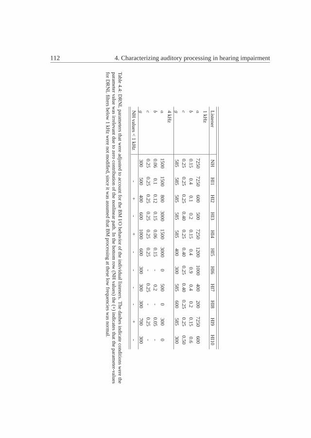
i

i

“MainFile” — 2010/7/15 — 15:31 — page 112 — #132i

i

i

i

i

i


ListenerN

HH

I1H

I2H

I3H

I4H

I5H

I6H

I7H

I8H

I9H

I10

1kH

za

72507250

600500

72501200

1000400

2007250

600b

0.150.4

0.10.2

0.150.4

0.90.4

0.20.15

0.6c

0.250.25

0.250.40

0.250.40

0.250.40

0.250.25

0.50g

585585

585585

585400

300585

600585

300

4kH

za

15001500

8003000

15003000

0500

0300

0b

0.060.1

0.120.15

0.060.15

-0.2

-0.05

-c

0.250.25

0.250.25

0.250.25

-0.25

-0.25

-g

300500

400600

1000600

300300

300700

300

NH

values<

1kH

z-

+-

+-

--

-+

-

Table4.4:

DR

NL

parameters

thatwere

adjustedto

accountfort

heB

MI/O

behaviorofthe

individuallisteners.T

hedashes

indicate

conditionsw

erethe

parameter

valuew

asirrelevantdue

tozero

contributionofthe

nonlinearpath.

Inthe

bottomrow

(NH

values)the

(+)

indicates

thattheparam

eter-valuesfor

DR

NL

filtersbelow

1kH

zw

erenotm

odified,sinceitw

asassum

ed

thatBM

processingatthese

lowfrequencies

was

normal.

i

i

“MainFile” — 2010/7/15 — 15:31 — page 113 — #133i

i

i

i

i

i

4.4 Results 113

HL

OH

CH

I1H

I2H

I3H

I4H

I5H

I6H

I7H

I8H

I9H

I10

0.25

kHz

1614

1010

14

1517

130

0.5

kHz

1122

78

1010

1523

88

1.0

kHz

121

221

1318

2429

117

2.0

kHz

1128

1015

1538

2538

1838

4.0

kHz

2228

2028

2043

3043

3643

8.0

kHz

3743

2546

2046

4646

4640

HL

IHC

HI1

HI2

HI3

HI4

HI5

HI6

HI7

HI8

HI9

HI1

00.

25kH

z4

160

039

260

287

150.

5kH

z14

138

1720

250

2212

171.

0kH

z19

148

1917

226

219

82.

0kH

z34

210

2015

715

2717

74.

0kH

z23

2210

75

1230

2224

78.

0kH

z23

1225

1410

3934

2919

0

Tabl

e4.

5:Va

lues

ofH

L OH

Can

dH

L IH

Cat

diffe

rent

freq

uenc

ies

deriv

edfr

omth

em

odel

sfit

ted

toth

ein

divi

dual

liste

ners

.

i

i

“MainFile” — 2010/7/15 — 15:31 — page 114 — #134i

i

i

i

i

i


ListenerN

HH

I1H

I2H

I3H

I4H

I5H

I6H

I7H

I8H

I9H

I10

−10-dB

BW

,roex,1kHz

(Hz)

300290

380410

330320

300410

300280

330−

10-dB

BW

,DR

NL,1kH

z(H

z)350

350380

390390

370270

360410

380400

Difference,1

kHz

(in%

)14

170

-515

14-11

-1428

2618

−10-dB

BW

,roex,4kHz

(Hz)

9401330

13801550

1520790

--

--

-−

10-dB

BW

,DR

NL,4kH

z(H

z)990

940850

730850

740-

--

--

Difference,4

kHz

(in%

)5

-42-62

-112-78

7-

--

--

SF

Mrm

sdiff.,1

kHz

(dB)

4.210.7

6.56.3

8.15.7

3.64.9

3.713.2

4.3S

FM

rms

diff.,4kH

z(dB

)6.3

6.13.4

5.67.9

7.34.2

1.76.0

12.75.9

Table4.6:

Results

ofthe

modelevaluation:

-10dB

bandwidthsfor

theroex-filters

andD

RN

Liso-intensity

responsesand

the

differencebetw

eenthe

bandwidths

inpercent;

andrm

sdifference

between

measured

and

simulated

thresholdsfor

thesim

ultaneous-and

forward

maski

ng(S

FM

)experim

ent.T

hedashes

indicateconditions

were

the-10-dB

BW

couldnotbe

obtained.F

orthe

BW

sa

differencebelow

20%w

asconsidered

reasonable,w

hilefor

theS

FM

experimentrm

sdifference

valueslow

erthan

8dB

were

considered

fairm

atches.

i

i

“MainFile” — 2010/7/15 — 15:31 — page 115 — #135i

i

i

i

i

i

4.5 Discussion 115

4.5 Discussion

4.5.1 Behavioral estimates of human BM input/output functions

In the present study, the TMC method was used to behaviorallyestimate individual

BM I/O functions. The results showed a large variability of knee-point position and

amount of compression among the HI listeners, even in the cases of similar pure-

tone sensitivity at the corresponding frequencies. These findings are consistent with

other studies (e.g.,Placket al., 2004; Lopez-Povedaet al., 2005; Rosengardet al.,

2005) which also found compression ratios for the HI listeners that ranged between

values of 0.15-0.25 dB/dB, as typically found in NH listeners, and values of one (i.e.,

linear processing), with considerable variation across the individual listeners. The

estimated parameters of the I/O functions found in the present study were consistent

with the measured frequency selectivity in the same individual listeners, i.e., losses

of compression were generally associated with a decreased frequency selectivity and

a shallower decay of forward masking curves, which agrees with earlier studies (e.g.,

Oxenhamet al., 1997; Moore et al., 1999). For some of the listeners of the present

study, it was not possible to obtain an estimate of the knee-point of the I/O function.

In these cases, only an estimate of the amount of compressioncould be derived

from the data and linear processing was assumed below the lowest measurable data

point. However, in other listeners and conditions, the knee-point could be estimated

and provided valuable additional information thus increasing the confidence in the

I/O function estimates. On the basis of the estimated I/O functions, the amount

of sensitivity loss due to OHC loss could be estimated in the individual listeners.

However, in the conditions were the knee-point estimate could not be obtained the

amount of OHC loss may be overestimated. If a knee point existed and was different

from the assumed value, then the difference would result in an overestimation of

OHC loss by an equal amount in dB. This, in turn, would lead to underestimated

IHC loss by the same amount, since this quantity was derived based on the OHC loss

estimate. It may be useful to have more robust psychophysical measures of the BM

knee point as e.g., suggested in Jepsen and Dau (2008) to overcome the present issue.

An earlier suggested method to obtain estimates of HLOHC was using a loudness-

model (Moore et al., 1999). In their study, it appeared that the estimated ERB only

i

i

“MainFile” — 2010/7/15 — 15:31 — page 116 — #136i

i

i

i

i

i


increased with increasing HLOHC when HLOHC was above 25 dB. This could reflect

that their loudness-based estimate of HLOHC is less reliable at the mild losses. In the

present study the listeners generally had less hearing lossthan those of the Moore et

al. study, and the presented correlation between HLOHC and ERB is compromised,

since very few ERB estimates was obtained for the severe losses.

As discussed in related recent studies (e.g.,Rosengardet al., 2005; Wojtczak and

Oxenham, 2009), the TMC method has several limitations.Rosengardet al. (2005)

found that the TMC data generally exhibit a larger variability than data obtained with

an alternative paradigm also based on forward masking, the growth of masking (GOM)

method (Oxenham and Plack, 1997). The GOM method varies the signal level and

keeps the masker-signal interval constant, which might provide a more stable cue for

the listeners of "when to listen" for the signal. Furthermore, the reliability of the

compression estimate has been found to be affected by the choice of the "linear" (off-

frequency) reference condition.Rosengardet al. (2005) further concluded that the

TMC method was less effective, since it was necessary to testa large range of masker-

signal intervals to measure in dynamic range of input levelsof interest. However, if the

original assumption on the off-frequency TMC representinga linear reference (Nelson

et al., 2001) is valid, then it is expected that the slope does not change due to reduced or

lost BM compression. The related earlier studies (Nelson and Carney, 2004; Placket

al., 2004; Lopez-Povedaet al., 2005; Rosengardet al., 2005; Wojtczak and Oxenham,

2009) discuss the origin of the observed shallower slope of the off-frequency TMC in

HI listeners. It could be due to reduced temporal resolutionin the HI listeners, since

the HI listeners were generally older than the NH listeners in these studies. It would be

expected that reduced temporal resolution would affect on-and off-frequency masking

by an equal amount. It is more likely that shallower off-frequency TMC are reflecting

that the necessary masker levels generally are higher for the HI listeners, and therefore

influence sources of forward masking other than BM processing, such as adaptation

and therefore lead to different rates of recovery from forward masking. Furthermore,

Wojtczak and Oxenham(2009) showed that the recovery from forward masking, with

on- versus off-frequency maskers adjusted to produce the same amount of masking at a

particular masker-signal interval, was different, especially at high masker levels. This

violates the basic assumption of the TMC paradigm which assumes a frequency and

i

i

“MainFile” — 2010/7/15 — 15:31 — page 117 — #137i

i

i

i

i

i

4.5 Discussion 117

level-independent recovery. As a consequence, compression might be overestimated

by the TMC method by a factor of two (Wojtczak and Oxenham, 2009). This would

of course have an impact on the results from this study, sincean overestimated

compression would imply an underestimated amount of OHC loss (derived from the

estimated I/O function) and would lead to too narrow tuning of the simulated BM

filters (discussed further below). However, also the alternative attempts to estimate

BM I/O function have their clear drawbacks and limitations (Wojtczak and Oxenham,

2009). For example, the GOM method does not provide reliable information about the

knee-point of the I/O functions, and might be influenced by off-frequency listening

due to the varying signal levels, and is also based on the assumption of a frequency

independent recovery from forward masking. Thus, the TMC method can still be

regarded as a reliable tool to behaviorally estimate BM I/O functions in humans.

The predicted slope of the off-frequency TMC mainly depended on the nonlinear

processing of the DRNL and adaptation stage within the model. The match between

the slope values at 1 kHz for the model of normal hearing reflects that the interaction

between these two can account for tone on tone forward masking which was expected

from the results ofJepsenet al. (2008). At 4 kHz, the predicted slope for NH was

slightly shallower than the data of this study, and consistent with slope estimates

of, e.g.,Lopez-Povedaet al. (2003). The model fitted to the individual HI listeners

generally produced a shallower and roughly constant slope of the off-frequency TMC.

These shallower slopes are primarily due to the processing of the adaptation stage.

The adaptation stage acts in a nonlinear way and higher inputlevels would lead

to a faster recovery of masking (Dau et al., 1996a,b; Jepsenet al., 2008). Faster

recovery of masking is expected to produce steeper TMCs. Within the presented

model the output of the early stages of the model, prior to theadaptation stage, is

reduced due to the simulation of OHC and IHC loss. Consequently, the adaptation

stage effectively processes the stimulus as if it was at a lower level and this leads

to a prediction of shallower slopes of the TMCs and differently for the on- and off

frequency conditions in the cases where residual BM compression is simulated. In

other studies, the shallower TMCs were discussed as being due to the general use of

higher masker levels for HI listeners (e.g.,Lopez-Povedaet al., 2005). The present

modeling efforts show that shallower slopes may not be due tothe use of high external

i

i

“MainFile” — 2010/7/15 — 15:31 — page 118 — #138i

i

i

i

i

i


masker levels, but due to a lower internal representation ofthe masker in models of

HI.

From a clinical and application-oriented perspective, though, the TMC method

might be unattractive because it is very time consuming. It would therefore

be interesting to investigate alternative behavioral methods such as, for example,

loudness scaling (with narrowband stimuli) in connection with predictions from

loudness models to estimate BM compression. While loudness growth functions are

relatively easy to assess, it is not clear to what extent suchmeasures can actually

estimate peripheral compression and estimates of OHC and IHC losses. Alternatively,

objective methods have been suggested to estimate BM properties, such as distortion-

product otoacoustic emissions (Williams and Bacon, 2005; Lopez-Povedaet al.,

2009). So far, however, this has only been tested in NH listeners and it is unclear

how reliable such measures are in HI listeners.

It remains unclear why this crossing of on- and off-frequency TMCs was observed

for particular listeners at some frequencies. One possibility could be related to the

tuning of the auditory nerve associated with SNHL.Liberman and Dodds(1984)

measured AN tuning in animals after noise trauma. They observed that the tails of

the AN tuning functions were hypersensitive at sites basal to the site of the trauma.

However, these observations were made in animals were the noise trauma were

induced locally by narrowband noise, and the hair cells at the relevant sites were

mainly intact. It is therefore questionable that this effect is a primary explanation

for the crossing TMCs, since the human listeners in the present study are unlikely to

have SNHL in very distinct region in the cochlea.

4.5.2 Evaluation of the models fitted to individuals

The models fitted to the individuals were evaluated in terms of predictions of data from

the experiments, as well as psychophysical measures derived from these data. Models

of auditory perception are most appropriately evaluated interms of its ability to predict

measured data. Additionally, measures derived from the data can be compared to the

processing of individual stages in the model. In the presentstudy, the model was

employed to predict the psychophysical data in terms of pure-tone sensitivity, off-

frequency TMCs, notched-noise masking and conditions of simultaneous and forward

i

i

“MainFile” — 2010/7/15 — 15:31 — page 119 — #139i

i

i

i

i

i

4.5 Discussion 119

masking using broadband maskers. Overall, these data were well accounted for.

However, the off-frequency TMCs were accounted for in termsof the slope of the

masking curve, and to a less degree the actual masker levels.In the notched-noise

masking experiment there was a general problem in simulating the masked thresholds

produced by the 4-kHz signal. Regarding the evaluation against derived measures,

the tuning of the DRNL stage fitted to the listeners was evaluated against roex filters

derived from the notched noise data. These results confirmedthat the tuning of the

model at 4 kHz was not well simulated.

4.5.3 Relationships between different measures in individual lis-

teners

The relationships between several quantities (absolute threshold, compression,

HLOHC , HLIHC , ERB) derived from the data showed a broad agreement with

the literature. Strong correlations were found between absolute threshold and

HLOHC. The correlation between absolute threshold and HLIHC was slightly weaker.

The relationship between compression and the three measures: absolute threshold,

HLOHC , HLIHC showed only weak correlations. Broadly the data indicates that

several of these quantities are not predictable from the absolute threshold and

strengthens the point that further individual characterization of cochlear hearing

loss is relevant. The relationships between the tested quantities and the ERB the

picture was in good agreement with the findings ofMoore et al. (1999), except that

the present data showed a weaker correlation between compression and the ERB. The

two studies share approximately the same amount of data points. The discrepancy

between the correlations may reflect that the Moore et al. study had more listeners

with severe hearing loss and estimates of compression higher than 0.7.

4.5.4 Capabilities and limitations of the modeling approach

The model framework has earlier been successfully applied to NH data in various

experimental detection and masking conditions (e.g.,Dau et al., 1996b, 1997a,b;

Verhey et al., 1999; Derleth and Dau, 2000; Piechowiaket al., 2007). Recently,

nonlinear effects associated with BM processing were included in this model (Jepsen

i

i

“MainFile” — 2010/7/15 — 15:31 — page 120 — #140i

i

i

i

i

i


et al., 2008) using the DRNL filterbank (Lopez-Poveda and Meddis, 2001). This

model was also considered here to predict effects of SNHL. However, in principle,

other cochlear front-ends could have been chosen alternatively, such as the auditory

nerve (AN) model ofHeinz et al. (2001a,c) and more recent implementations of

it (e.g., Bruce et al., 2003). One focus of their modeling has been to account for

IHC and OHC losses. For example,Bruceet al. (2003) assumed that OHC function

is responsible for the active gain mechanism and for BM tuning while the function

of the IHCs is primarily a transduction of information to theAN. They simulated a

more linear BM response, less gain and broadened tuning withincreasing OHC loss.

The maximum OHC gain in their model was 46 dB which also reflects the largest

possible effect of OHC loss in their model in terms of sensitivity loss. Their model

used a single parameter to simulate the effect of OHC loss, and allowing only one

parameter to control the I/O behavior due to OHC damage may betoo restrictive,

and may not provide the necessary flexibility to capture individual BM I/O behavior

in listeners with SNHL. In the present study, four parameters were adjusted and this

leads to more flexibility in term of fitting I/O function to data in terms of, e.g., knee

point and compression, with the cost of a more complex and less straight-forward

procedure. InBruceet al. (2003); Zilany and Bruce(2006) their simulated IHC loss

leads to reduced sensitivity and does not affect the model’stuning and compression.

This approach is thus conceptually similar to the one used inthe present study. The

dynamic compressive gammachirp filter, suggested byIrino and Patterson(2006),

provides another peripheral filtering simulation stage, but it is not clear how the model

can be modified to implement changes in the I/O function to account for hearing loss.

The multi-bandpass nonlinear filter ofGoldstein(1990) has a very similar structure as

the DRNL filter, but it is unclear if the model’s I/O behavior can be modified without

disrupting other important properties of that particular model. Overall, the DRNL

filterbank was chosen here because of its computational efficiency and the possibility

to relatively easily modify the BM filters’ input-output characteristic to account for

hearing loss (Lopez-Poveda and Meddis, 2001).

While the earlier studies (e.g.,Dau et al., 1997a; Verheyet al., 1999; Jepsenet

al., 2008) were focused on the simulation of average NH data, one important aspect

of the present work was to provide a tool that allows to quantitatively account for the

i

i

“MainFile” — 2010/7/15 — 15:31 — page 121 — #141i

i

i

i

i

i

4.5 Discussion 121

variability in the HI data (whereas NH listeners typically show much less variability).

Specifically, the present study tried to evaluate and quantitatively predict the relations

between the results obtained in the TMC experiment, the frequency and temporal

resolution tasks and the audibility test in more detail thanearlier studies. The current

model provided a good overall description of the NH and HI data. Based on the

fitted I/O functions and the audiograms, OHC and IHC losses were estimated, and the

simulations showed how absolute sensitivity loss is related to supra-threshold deficits

within the framework of the model. The modeling results support the importance of

individual characterization of SNHL based on separate estimates of OHC and IHC

losses. However, the adjusted parameters were based on datacollected at only 1 and

4 kHz. Similar data could be obtained at more frequencies to gain more confidence

in the used cochlear model parameters. The use of interpolation and extrapolation of

the parameters at other DRNL filterbank frequencies may prove to be a too crude

assumption. It should be noted that to simulate the estimated BM I/O function,

there may exist another set of DRNL parameters (a, b, c andg) providing a similar

DRNL I/O function, since their interaction is nonlinear. The parameter-sets presented

here are thus not unique, but they reflect a suggestion following the manual fitting

procedure. The estimated values of HLIHC was derived from the measured audiogram

and the estimated HLOHC . This was done at discrete frequencies. In Fig.4.3 it

was observed that the predicted audiogram were not exactly fitting the measured

audiograms. The value of HLIHC could alternatively have been adjusted to fit the

measured audiograms. The predictions are, however, depending on the processing in

neighboring channels, such that the adjustment procedure would become less straight-

forward.

Regarding intensity resolution, the model predicted an essentially constant JND

across the simulated hearing-impaired listeners, which was not consistent with the

results for some of the HI listeners who clearly showed increased JNDs. The finding

of a constant intensity JND in the model, independent of the amount of peripheral

compression, is a consequence of the roughly logarithmic overall compression in

the (perception) model, as discussed in detail inJepsenet al. (2008). Thus, in this

framework, no effects of SNHL were expected in terms of intensity JNDs. This means

that either the assumptions regarding intensity coding in the model are inappropriate,

i

i

“MainFile” — 2010/7/15 — 15:31 — page 122 — #142i

i

i

i

i

i


or other sources of variability, potentially of retro-cochlear origin, need to be assumed

in order to explain the increased JNDs in some of the listeners. The model of normal

hearing could not predict the near miss to Weber’s Law (Jepsenet al., 2008). This

effect (observed in data) may be due to the integration of information across peripheral

channels, and may not be accounted for in the current modeling framework. If the

elevated JNDs observed in the present data for HI listeners reflect a lack of account for

the near miss to Weber’s Law, then this modeling framework was again not expected

to predict the observed data. In the framework of this model,an increased JND could

effectively be simulated by increasing the variance of the internal noise. However,

more specific hypotheses about potential sources for the limitations would be needed

as well as more knowledge about how such limitations might beaccounted for in an

auditory model.

The presented model in its current form has several limitations. First of all,

it was observed that the tuning of the DRNL filters fitted to listeners with mild-to-

moderate losses at 4 kHz was generally too sharp,both in relation to the prediction of

notched noise data, and evaluating the DRNL tuning to roex filters fitted to the data.

The tuning was determined by the simulated BM compression atthe corresponding

levels. For these listeners, residual compression was found at mid-to-high frequencies

and, consequently, a near-normal DRNL filter tuning was simulated. The reason

could indeed be that the amount of compression was overestimated by the TMC

method, as discussed above. Less compression in the DRNL filters would lead

to a broader tuning. It is, however, unclear why this problemwas only observed

at 4 kHz and not at 1 kHz. The discrepancy in the matches at 4 kHzcould

potentially affect future applications of the model of SNHL. If the model generally

simulate a too good frequency resolution at high frequencies, then the subjective

performance in complex tasks might be overestimated if the task reflects an influence

of reduced frequency selectivity. The results might also suggest that auditory filter

widths, as estimated by notched-noise masking, may not be solely determined by the

BM compression. Peripheral suppression has also been shownto affect frequency

selectivity in simultaneous notched-noise masking (e.g.,Sheraet al., 2002; Oxenham

and Shera, 2003) and suppression appears to be reduced with SNHL (e.g.,Heinz et

al., 2002). Two-tone suppression is included in the DRNL model but itseffects on

i

i

“MainFile” — 2010/7/15 — 15:31 — page 123 — #143i

i

i

i

i

i

4.5 Discussion 123

frequency selectivity in a notched-noise masking paradigmhave not been investigated

explicitly yet. The results might also suggest that auditory filter widths, as estimated

by notched-noise masking, may not be solely determined by the BM compression.

Additional contributors could be the shape of the assumed middle-ear transfer function

and/or changes at later stages of processing in the HI listeners.

Second, no temporal processing deficits in terms of the coding of temporal fine

structure (TFS) have been considered. Recently, the processing of TFS information

has been discussed intensively, particularly in connection with speech reception in

noise (e.g.,Lorenziet al., 2006; Strelcyk and Dau, 2009). TFS information typically

refers to the temporal fine structure at the output of the cochlear filters and this fine

structure evokes phase-locked activity, i.e. synchronized timing of action potentials in

the subsequent stages of neural processing (e.g.,Ruggero, 1992). Evidence for TFS

processing deficits in HI listeners has been found in previous studies of monaural as

well as binaural auditory functions. Several factors mightcontribute to the deficits

in TFS processing. A loss of OHCs could lead to a reduced precision of phase

locking (Woolf et al., 1981) even though this is controversial since other studies

have not found any physiological of SNHL on TFS coding (e.g.,Harrison and Evans,

1979; Miller et al., 1997). Alternatively, TFS deficits might also be attributable to

damage to or loss of auditory nerve fibers or the innervated IHCs (e.g.,Schuknecht

and Woellner, 1953). In terms of modeling, several studies have suggested that

the extraction of spatiotemporal information, i.e. the combination of phase-locked

responses and systematic frequency-dependent delays along the cochlea (associated

with the traveling wave), is important in the context of pitch perception (e.g.,Loebet

al., 1983), localization (e.g.,Shamma, 2001), speech formant detection (e.g.,Deng

and Geisler, 1987) and tone-in-noise detection (Carneyet al., 2002). It has been

proposed that a distorted spatiotemporal response might be, at least partly, responsible

for the problems of HI listeners to process TFS information across frequencies (e.g.,

Moore, 1996; Heinz and Swaminathan, 2009). In the present study, OHC and IHC

losses have only been considered in terms of associated sensitivity losses but not in

terms of temporal coding. Thus, consequences of TFS loss cannot be accounted for

by this model.

i

i

“MainFile” — 2010/7/15 — 15:31 — page 124 — #144i

i

i

i

i

i


4.5.5 Perspectives

Reedet al. (2009) reviewed a number of studies where SNHL was simulated by

adding threshold-shaped noise to the stimuli presented to NH listeners. Some of

these studies demonstrated that data on temporal processing, such as gap detection,

can be accounted for by adding noise masking (e.g.,Florentine and Buus, 1984).

In other experiments, such as temporal integration, this relation was not found (e.g.,

Florentineet al., 1988). It is not fully understood how additive external noise affects

the processing in the cochlea. The noise might linearize theBM response since higher

input levels are used such that the system operates similarly as in the case of a (severe)

SNHL. This could be tested by adding low-to-moderate level background noise while

estimating BM compression in comparison to a quiet condition. It may also be found

that the BM response does not change significantly with additive external noise.

The model presented here might be useful to explicitly investigate the effect of the

additional noise in the various experimental conditions and could help relating the

different findings to each other.

It would also be interesting to investigate more complex tasks, such as speech

perception in noise, which also depend on spectral and temporal resolution of the

auditory system. Models of speech intelligibility, e.g., the speech intelligibility

index (SII;ANSI, 1997), typically consider only aspects of reduced sensitivity;thus,

individual differences resulting from supra-threshold deficits are not accounted for.

Using the present model as a front-end in speech intelligibility predictions might thus

provide further insights into how HI listeners process speech sounds.

i

i

“MainFile” — 2010/7/15 — 15:31 — page 125 — #145i

i

i

i

i

i

4.6 Conclusions 125

4.6 Conclusions

• Audiometric pure-tone sensitivity, cochlear compression, frequency selectiv-

ity, intensity discrimination and temporal resolution were measured in ten

sensorineural hearing-impaired listeners. Considerabledifferences of the

results across the listeners were observed even for those listeners with similar

audiograms.

• The cochlear processing stage of the considered model framework was adjusted

to account for the individual behaviorally estimated BM input/output functions

and the audiograms. The model was evaluated in the experiments of frequency

selectivity, forward masking and intensity discrimination. The predictions of

the experimental data reflected the variability observed inthe experimental

data across listeners, as well as for the results obtained inthe normal-hearing

listeners. However, the model generally overestimated theamount of frequency

selectivity at 4 kHz for the listeners with mild-to-moderate hearing loss which

might be resulting from an overestimation of cochlear compression via the

temporal masking curve paradigm. Furthermore, the model predicted a roughly

constant intensity discrimination threshold across all listeners whereas the data

showed increased thresholds in some of the HI listeners.

• Overall, the results support the importance of an individual characterization

of (sensorineural) hearing impairment. The presented modeling framework

might also be useful for future investigations of effects ofindividual hearing

impairment on speech intelligibility in various experimental conditions and

could further be beneficial for the evaluation of compensation strategies and

signal-processing algorithms in hearing instruments, where listening tests are

time consuming and expensive.

i

i

“MainFile” — 2010/7/15 — 15:31 — page 126 — #146i

i

i

i

i

i


4.7 Appendix: Additional information about the lis-

teners

This appendix describes additional information about the hearing-impaired listeners

that were used in Chapter 4 and is listed in Table4.7. The etiologies of the hearing

losses are listed, and they are based on clinical diagnoses.It is also listed whether the

listeners were hearing-aid users or not. Finally, results from a speech intelligibility

test are listed. These results were not used or analyzed in the chapter, but are reported

here to make these data available to possible future studies.

Speech reception thresholds (SRTs) were measured for Danish Dantale II

sentences in three noise conditions. It is a closed-set wordrecognition test using

Hagerman sentences (Wageneret al., 2003). The noise conditions were: (1) stationary

speech-shaped noise (SSN) with the long-term spectrum of the Dantale II sentences;

(2) sinusoidally amplitude modulated (SAM) noise with a constant modulation rate

at 8 Hz and a modulation depths of 1; (3) randomly amplitude modulated (RAM)

noise was randomly modulated with the Hilbert envelope of a bandpass-noise (4 to

12 Hz) as modulator, which reflect typical modulation rates in running speech. The

modulation depth was 1. The SRT was defined as the SNR at which 50% words were

identified correctly. The noise level was constant while thelevel of the sentences was

varied adaptively. Listeners were trained on a single run with 20 sentences before

measurements were made. The reported SRTs are averages of two measurements.

The mean SRT results of the seven NH listeners used in Chapter3 are also given in

the table.

i

i

“MainFile” — 2010/7/15 — 15:31 — page 127 — #147i

i

i

i

i

i

4.7 Appendix: Additional information about the listeners 127

Listener Etiology Hearing-aid user SSN SAM RAMHI1 Presbycusis No -4.5 -7.7 -6.1HI2 Noise induced Yes -5.6 -6.4 -4.8HI3 Presbycusis Yes -4.2 -10.5 -6.1HI4 Presbycusis No -6.7 -9.2 -7.7HI5 Unknown No -5.8 -9.4 -6.9HI6 Unknown Yes -6.5 -9.3 -7.5HI7 Presbycusis Yes -4.8 -10.0 -6.9HI8 Presbycusis Yes 2.2 1.8 2.0HI9 Presbycusis Yes -3.2 -5.8 -4.2HI10 Unknown Yes -4.6 -7.0 -6.1Mean NH -7.6 -16.7 -10.7

Table 4.7: Additional information about the ten HI listenersused in Chapter 4. The table lists theirhearing loss etiology, hearing aid use and SRTs (in dB) in noise condition of stationary speech-shapednoise (SSN), Sinusoidally amplitude modulated (SAM) noise and an amplitude modulated noise with arandom modulation rate (RAM).

i

i

“MainFile” — 2010/7/15 — 15:31 — page 128 — #148i

i

i

i

i

i


i

i

“MainFile” — 2010/7/15 — 15:31 — page 129 — #149i

i

i

i

i

i

5Relating individual consonant

confusions to auditory processing inlisteners with cochlear damage6

Reduced sensitivity to sounds represents only one typical consequence ofhearing impairment. Additional factors such as spectral and temporalresolution have been considered to characterize (individual) hearing loss.The present study investigated consequences of deficits in auditory signalprocessing and the perception of speech sounds in individual listeners. First,psychophysical forward-masking data were obtained and theparametersof a peripheral auditory model were adjusted accordingly tosimulate theindividual listeners’ cochlear processing. Second, the same individuals weretested in a Diagnostic Rhyme Test (DRT). These stimuli were processedby the peripheral model obtained in the first phase. The resulting internalauditory representation was analyzed by a detector and error patterns werepredicted along the acoustic-phonetic dimensions of the DRT. An importantfeature of the DRT framework using synthesized diphones wasthe separationof errors originating from the periphery and detector, respectively. Mosterror patterns were accounted for by the model, providing a link betweenthe speech and non-speech data in hearing-impaired listeners. Error patternswere further predicted by a model which simulated reduced sensitivity only.It was found that this model produced too few errors and indicated that supra-threshold deficits have an influence on consonant confusionsin hearing-impaired listeners.

5 This chapter represents a journal article manuscript in preparation. The data and preliminary modelingresults were presented at the International Symposium on Auditory and Audiological Research(ISAAR), Helsingør, Denmark, 2009.

129

i

i

“MainFile” — 2010/7/15 — 15:31 — page 130 — #150i

i

i

i

i

i

130 5. Consonant confusions and cochlear damage

5.1 Introduction

A major concern of hearing-impaired (HI) people is their reduced ability to reliably

communicate through speech. Some are more handicapped in their communication

than others, depending on the type and salience of their hearing impairment. Even

people with similar a hearing loss, in terms of audibility, can differ greatly in their

ability to understand speech, particularly in complex acoustic environments with

background noise, reverberation or multiple sound sources. Hearing aids can restore

audibility by amplifying speech signals and can improve thespeech-to-noise ratio

(SNR) by different techniques, such as directional microphones and noise reduction

schemes. However, the benefit from the available technical solutions differ in

individual hearing-aid users. For some people, the hearingaids restore the ability

to function almost normally in every-day communication, while others report only

limited or no benefit from hearing aids, particularly in challenging situations. It is

of great importance to obtain a better understanding of how the processing of speech

sounds is affected by the individual hearing impairment in order to identify the sources

of the variability in the speech-in-noise perception data across listeners.

spects of hearing impairment which are not accounted for by sensitivity loss

are referred to as supra-threshold deficits, such as loudness recruitment, reduced

frequency selectivity and reduced temporal resolution which also are typical conse-

quences of a sensorineural hearing loss.Moore et al. (1999) and Jepsen and Dau

(2010) showed that even hearing-impaired listeners with comparable audiograms can

show large differences in their performance in tasks related to supra-threshold deficits.

The differences may be associated with individual patternsof outer hair-cell (OHC)

and inner hair-cell (IHC) damages (Jepsen and Dau, 2010; Lopez-Povedaet al.,

2009). Frequency selectivity, temporal resolution and intensity resolution are usually

measured by psychoacoustic experiments using synthetic non-speech stimuli such as

tones presented in noise maskers. It is unclear how these deficits are reflected in

psychoacoustic tasks with more natural stimuli such as speech. Linking speech and

non-speech psychophysics might provide a step towards a better understanding of the

variability observed, particularly in the speech data of HIlisteners.

Jepsen and Dau(2010) modified some of the parameters of computational

i

i

“MainFile” — 2010/7/15 — 15:31 — page 131 — #151i

i

i

i

i

i

5.1 Introduction 131

auditory signal-processing and perception (CASP) model (Jepsenet al., 2008) on

the basis of estimated basilar-membrane (BM) input-output(I/O) function and the

audiogram. This was done on an individual basis for ten listeners with cochlear

hearing loss, and individual differences were associated with differences in the

estimates of OHC and IHC loss. Their model accounted for supra-thresholds deficits

such as broader auditory filters and reduced temporal resolution as well as reduced

sensitivity. An earlier version of the CASP model has earlier been used as a front

end in studies involving speech stimuli.Holube and Kollmeier(1996) considered the

model of auditory perception fromDau et al. (1996a) as the front end and derived

an intelligibility index. They accounted for the reduced intelligibility of speech in

noise for NH and HI listeners.Holube and Kollmeier(1996) simulated effects of

hearing loss due to audibility and frequency selectivity, however, these aspects were

not simulated as a direct consequence of cochlear compression as suggested inJepsen

and Dau(2010). The same perception model front-end was used in an automatic

speech recognizer system inTchorz and Kollmeier(1999) with a Hidden-Markov

Model (HMM) back end, where it was shown that higher robustness to noise was

obtained using the auditory processing front end compared to the commonly used

mel-scale cepstral coefficient feature extraction. However, due to the HMM back

end it cannot be concluded whether the robustness is obtained due to the front-end

processing alone.

Models of the auditory periphery attempt to appropriately describe a perceptually

relevant "internal representation" (IR) of the incoming sounds. To investigate whether

the simulated IR provides a good match to the “real” IR, it is crucial that front-end and

back-end processing, for example in a speech recognition system, are clearly separated

(Ghitza, 1993). The ultimate goal is not to obtain perfect speech recognition but to

match human performance, and thereby to contribute to a better understanding of how

speech is processed in the auditory system.Ghitza(1993) suggested that the cognitive

component involved in consonant recognition (both for humans and machines) could

be minimized by using the diagnostic rhyme test (DRT;Voiers, 1983), because this

test represents a simple binary discrimination task. However, their back-end stage

was found to be a source of errors since a HMM was used as a recognizer, even after

attempts were made to keep its errors at a minimum.Messinget al. (2009) proposed

i

i

“MainFile” — 2010/7/15 — 15:31 — page 132 — #152i

i

i

i

i

i


a modeling framework to predict confusion patterns from DRTin NH listeners, where

they further separated the peripheral model (front end) andthe detector stage (back

end) by using synthesized DRT diphones. These allowed them to use of a simple back

end which measures a perceptual distance to templates in order to keep the back-end

errors at a minimum. Their framework and data was used to measure inaccuracies in

the front-end model’s internal representation of speech.

The goal of the present study was to investigate how degradedauditory

processing, due to cochlear damage, affects speech perception in individual listeners.

This was done in the framwork of the synthesized DRT, using the CASP model (Jepsen

et al., 2008; Jepsen and Dau, 2010) as the front end and a detector similar to that

of Messinget al. (2009) as the back end. The separation of front-end and back-

end processing was of conceptual importance here, since predicted errors could thus

be uniquely associated with the front-end processing and could provide a measure

of how well the CASP model, including the simulation of cochlear hearing loss,

can describe the actual IR of speech sounds in individual hearing-impaired listeners.

For the simulation of hearing impairment, the front end was fitted to the individual

listeners due to non-speech psychophysics, based on behavioral estimates of BM

I/O functions and the audiogram following the method suggested inJepsen and Dau

(2010). The peripheral model then remained unchanged for the simulations of DRT

error patterns. If the model was able to predict individual error patterns in the DRT

task based on individual fits to the non-speech tasks, then degraded performance in

the speech tasks could be associated with limitations in basic auditory processing in

the individuals. In order to resolve whether simulated DRT errors were accounted for

due to reduced sensitivity (audibility) alone, individualerror patterns were simulated

using a configuration of the CASP model which only simulated reduced sensitivity

without changing the BM processing stage.

A common measure of speech intelligibility is the speech reception threshold

(SRT), which is a single value typically defined as the SNR at which 50% of a sentence

is correctly understood. HI listeners commonly have higherSRTs than NH listeners,

i.e., they need a larger SNR to recognize speech. The SRT depends critically on

experiment-specific factors, such as speech material, background-noise characteristics

as well as specific characteristics of the hearing loss. SRT measurements provide a

i

i

“MainFile” — 2010/7/15 — 15:31 — page 133 — #153i

i

i

i

i

i

5.1 Introduction 133

useful tool to study the influence of a specific noise-type or atransmission channel on

speech intelligibility or to roughly quantify the communication difficulties of hearing-

impaired listeners. However, a SRT value does not reveal information about which

elements of the speech that were received incorrectly and what the source of the errors

was, for example in terms of specific hearing impairment factors.

Other experiments using speech stimuli have been designed to obtain more

detailed information about speech perception. One exampleis the DRT (Voiers, 1983),

used in the present study, where consonant confusions can bemeasured by consonant

discrimination along a number of acoustic-phonetic features. Another example is

the approach described inMiller and Nicely (1955) where consonant recognition is

measured (at different SNRs) and consonant confusion patterns can be derived from

the data. This allows categorizing typical confusions in terms of perceptual features.

Phatak and Allen(2007) andPhataket al. (2008) extended the analysis of consonant

confusion patterns and provided a detailed analysis in terms of perceptual consonant

groups.

Speech perception models have been useful, for example for evaluating the effect

of room acoustics on speech intelligibility. The articulation index (e.g.,Kryter, 1962;

ANSI, 1969) and later the speech intelligibility index (SII;ANSI, 1997) provide

estimates of the expected average speech intelligibility of a signal that has been

distorted by a transmission-line. The SII also includes a component that addresses

hearing impairment, but only the loss of sensitivity is considered. The speech

transmission index (STI;Steeneken and Houtgast, 1980), is based on the distortion

of the modulation depth through a transmission channel, such as a reverberant room.

There are no standardized procedures to account for hearingloss in the STI method,

but some attempts have been made to address this issue (Humeset al., 1986). More

recently,Elhilali et al.(2003) presented a model that analyzes (joint) spectra-temporal

modulations in the signal to predict speech intelligibility. They introduced the measure

of the spectro-temporal modulation index (STMI) which could account for effects of

degraded temporal modulations in a similar way as the STI, but could further describe

effects of nonlinear distortions on speech intelligibility which degraded the pattern of

spectral periodicities (spectral modulation).

In this study, the representation of speech sounds in the CASP model was used to

i

i

“MainFile” — 2010/7/15 — 15:31 — page 134 — #154i

i

i

i

i

i


predict the DRT error patterns of listeners with cochlear hearing loss. The hypothesis

was that an appropriate simulation of sensitivity loss and supra-threshold deficits is

required to account for individual differences in the errorpatterns measured in the

same individuals.

i

i

“MainFile” — 2010/7/15 — 15:31 — page 135 — #155i

i

i

i

i

i


5.2 Experimental methods

5.2.1 Listeners

Three listeners with mild-to-moderate sensorineural hearing loss participated in this

study. Listeners S1, S2 and S3 were 21, 45 and 27 years old, respectively. All these

have had a hearing loss since their early childhood. S1 and S2were regular users of

hearing aids while S3 did not use hearing aids. Only one ear ofeach listener was

measured in the speech and non-speech tasks. The audiogramsof the measured ears

are shown in Fig.5.1 (open symbols). The listeners were selected to have hearing

losses less than 55 dB HL at frequencies from 0.25 to 4 kHz. Therationale behind this

choice was to be able to measure performance in the speech task without compensating

for audibility and thereby potentially introducing undesired distortion. The listeners

were paid for their participation on an hourly basis. Measurement appointments lasted

two hours and sessions had durations of about 30 to 45 minutes. Training sessions in

the forward masking task were run until no systematic improvements were observed,

usually after two to four hours. For the DRT, three hours of training were provided.

The total testing time for each subject was about 16 to 20 hours, including training.

.25 .5 1 2 4 8

100

80

60

40

20

0

S1Thr

esho

ld (

dB H

L)

.25 .5 1 2 4 8

S2

Frequency (kHz).25 .5 1 2 4 8

S3

Sim.

Data

Figure 5.1: Audiograms of the measured ears of the three HI listeners. Pure-tone thresholds are plotted indB hearing level (HL). Open symbols indicate measured thresholds, while filled symbols indicate simulatedthresholds by the corresponding models (described in Sec.5.4).

i

i

“MainFile” — 2010/7/15 — 15:31 — page 136 — #156i

i

i

i

i

i


5.2.2 Apparatus

Audiograms were provided by audiological clinics while allother data were collected

in the laboratory of the Biomedical Engineering departmentat Boston University.

The stimuli were presented monaurally to the subject via headphones (Sennheiser

HD265) in a sound-insulated listening booth. Listeners responded on a computer

keyboard, following the instructions on a computer monitorlocated in the booth. The

experiments were run on a personal computer with a 16-bit high-quality soundcard.

5.2.3 Temporal masking curves (TMC)

In the TMC experiment, forward masking of a fixed-level brieftone was measured as

a function of signal-masker interval. The probe signal was apure tone with a duration

of 20 ms, which was Hanning windowed over its entire duration. The frequency (fsig)

was either 1 or 4 kHz. The signal was presented at 10 dB sensation level (SL). The

masker was also a pure tone with a duration of 200 ms including5-ms raised-cosine

on- and off ramps. The masker frequency (fm) was equal tofsig (on-frequency

condition) or0.6 ·fsig (off-frequency condition). The masker-signal interval was 2, 5,

10 ms and additional 10-ms increments until the subject reported (in pilot runs) that

the masker level became uncomfortably loud, or reached the maximum level of 95 dB

SPL. Stimuli were generated in Matlab at a sampling rate of 44.1 kHz. The masker

level was adjusted by the adaptive procedure to reach maskedsignal threshold. A

three-interval tree-alternative forced choice paradigm in connection with a two-up-

one-down rule were applied. The reported thresholds reflectthe 70.7% point on the

psychometric function and represent the mean of at least three measured thresholds.

The step size was varied adaptively, starting at 8 and endingat 1 dB, and thresholds

were an average of the levels at the last eight reversals withthe final step size. The

listener received immediate feedback on whether a responsewas correct or not.

5.2.4 The diagnostic rhyme test (DRT)

The DRT of Voiers (1983) uses 192 minimal pair diphones and was designed to

cover six acoustic-phonetic dimensions: voicing (VC), nasality (NS), sustention

(ST), sibilation (SI), graveness (GV) and compactness (CM). The diphones were

i

i

“MainFile” — 2010/7/15 — 15:31 — page 137 — #157i

i

i

i

i

i


synthesized by a text-to-speech system, such that the acoustic waveforms only differed

in the initial consonant. The test stimuli had a sampling rate of 16 kHz and were

identical to those used inMessinget al.(2009). The noise was a Gaussian noise which

was spectrally shaped to have a long-term spectrum similar to speech. Different noise

tokens were realized in the generation of the noisy stimuli.The speech had a constant

rms level of 70 dB SPL and was presented in background noise at SNRs of 0 and 10

dB. Eight repetitions of the 192 diphones were presented in blocks of 128 in random

order. The DRT is a binary consonant discrimination task realized in a one-interval

two-alternative forced-choice method. The listeners werenot given feedback on their

responses. The performance of the listeners was evaluated by the error rate along the

six acoustic-phonetic dimensions. Examples of minimal pairs are given in Table5.1

(see also,Voiers, 1983; Ghitza, 1993).

i

i

“MainFile” — 2010/7/15 — 15:31 — page 138 — #158i

i

i

i

i

i


Voicing (VC) Nasality (NS) Sustention (ST)Voiced - Unvoiced Nasal - Oral Sustained - Interrupted

veal - feel meat - beat vee - beebean - peen need - deed sheet - cheatgin - chin mitt - bit vill - billdint - tint nip - dip thick - tickzoo - Sue moot - boot foo - pooh

dune - tune news - dues shoes - choosevole - foal moan - bone those - dozegoat - coat note - dote though - doughzed - said mend - bend then - den

dense - tense neck - deck fence - pencevast - fast mad - bad than - Dangaff - calf nab - dab shad - chad

vault - fault moss - boss thong - tongdaunt - taunt gnaw - daw shaw - chawjock - chock mom - bomb von - bonbond - pond knock - dock vox - box

Sibilation (SB) Graveness (GV) Compactness (CM)Sibilated - Assibilated Grave - Acuté Compact - Diffuse

zee - thee weed - reed yield - wieldcheep - keep peak - teak key - tea

jilt - gilt bid - did hit - fitsing - thing fin - thin gill - dilljuice - goose moon - noon coop - poopchew - coo pool - tool you - rue

Joe - go bowl - dole ghost - boastsole - thole fore - thor show - sojest - guest met - net keg - pegchair - care pent - tent yen - wrenjab - dab bank - dank gat - bat

sank - thank fad - thad shag - sagjaws - gauze fought - thought yawl - wallsaw - thaw bong - dong caught - taught

jot - got wad - rod hop - fopchop - cop pot - tot got - dot

Table 5.1: Examples of diphone minimal pairs in the six acoustic-phonetic features. Each feature-blockcontains 16 minimal pairs, thus there are 192 diphones in total.

i

i

“MainFile” — 2010/7/15 — 15:31 — page 139 — #159i

i

i

i

i

i

5.3 Modeling speech perception 139

5.3 Modeling speech perception

5.3.1 The front end

A schematic structure of the front-end, the CASP model (Jepsenet al., 2008; Jepsen

and Dau, 2010), is shown in Fig.5.2. The acoustic stimuli are first processed

by the outer- and middle ear filters, followed by the dual-resonance nonlinear

(DRNL) filterbank (Lopez-Poveda and Meddis, 2001) simulating BM processing. The

processing of the subsequent stages is carried out in parallel in the frequency channels.

Inner hair-cell transduction is modeled roughly by half-wave rectification followed by

a first-order lowpass filter with a cut-off frequency at 1 kHz.The expansion stage

transforms the output of the IHC stage into an intensity-like representation by applying

a squaring expansion. The adaptation stage simulates dynamic changes in the gain of

the system in response to changes in the input level. It consists of five feedback loops

with time-constants in the range from 5 to 500 ms. For a stationary input signals,

the output approaches a logarithmic compression. For rapidinput variations the

transformation through the adaptation loops is more linear, leading to an enhancement

in fast temporal variations, such as onsets. The output of the adaptation stage is

processed by a first-order lowpass filter with a cut-off frequency at 150 Hz, followed

by the modulation filterbank, which is a bank of bandpass filters tuned to different

modulation frequencies (Dau et al., 1997a). For further details on the CASP model

stages, the reader is referred to (Jepsenet al., 2008) and (Jepsen and Dau, 2010).

5.3.2 Simulation of individual hearing loss

Jepsen and Dau(2010) described a method to adjust the parameters of the cochlear

stages of the model (DRNL filterbank and hair-cell transduction, gray blocks in

Fig. 5.2 to simulate degraded processing due to hair-cell loss. The I/O function of

the DRNL filters simulating normal hearing has a linear low-level part for input levels

below about 30-40 dB SPL, whereas compressive processing isassumed above this

level. The transition between the linear and the compressive region is referred to as the

knee point. Here, the I/O behavior of the DRNL filterbank was adjusted to correspond

to the BM I/O functions estimated behaviorally in the three HI listeners, in terms of the

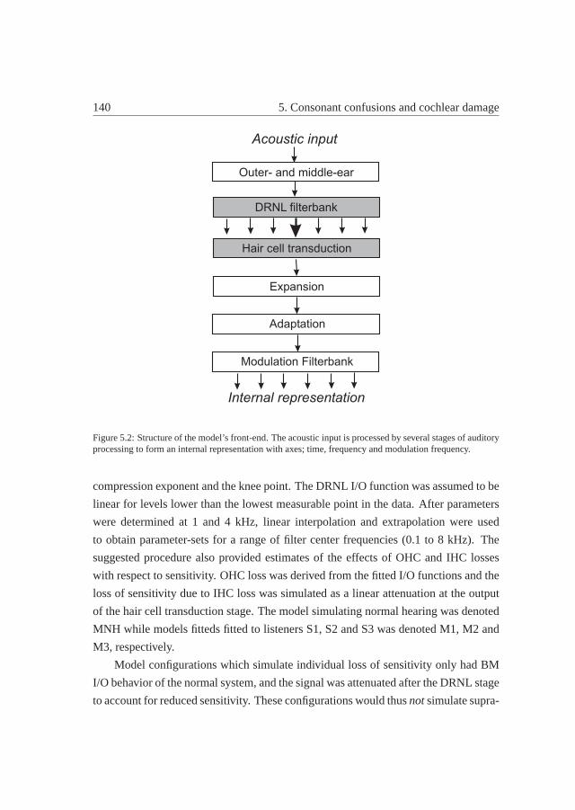
i

i

“MainFile” — 2010/7/15 — 15:31 — page 140 — #160i

i

i

i

i

i



Expansion

Adaptation

Outer- and middle-ear

DRNL filterbank

Modulation Filterbank

Internal representation

Acoustic input

Figure 5.2: Structure of the model’s front-end. The acousticinput is processed by several stages of auditoryprocessing to form an internal representation with axes; time, frequency and modulation frequency.

compression exponent and the knee point. The DRNL I/O function was assumed to be

linear for levels lower than the lowest measurable point in the data. After parameters

were determined at 1 and 4 kHz, linear interpolation and extrapolation were used

to obtain parameter-sets for a range of filter center frequencies (0.1 to 8 kHz). The

suggested procedure also provided estimates of the effectsof OHC and IHC losses

with respect to sensitivity. OHC loss was derived from the fitted I/O functions and the

loss of sensitivity due to IHC loss was simulated as a linear attenuation at the output

of the hair cell transduction stage. The model simulating normal hearing was denoted

MNH while models fitteds fitted to listeners S1, S2 and S3 was denoted M1, M2 and

M3, respectively.

Model configurations which simulate individual loss of sensitivity only had BM

I/O behavior of the normal system, and the signal was attenuated after the DRNL stage

to account for reduced sensitivity. These configurations would thusnotsimulate supra-

i

i

“MainFile” — 2010/7/15 — 15:31 — page 141 — #161i

i

i

i

i

i


thresholds deficits due hair-cell loss. These model configuration were denoted A1, A2

and A3, respectively. These are also referred to as the "sensitivity-only" models.

5.3.3 Internal representation of the stimuli after auditory process-

ing

The output of the preprocessing stages, the internal representation (IR) of the

respective input stimulus, has the dimensions time (t), frequency (f ) and modulation

frequency (mf). IRs were generated using DRNL filters in the range from 0.1 to 8

kHz, with 4 filters per equivalent rectangular bandwidth (60channels in total) and

considering the first six modulation filters, with modulation filter center frequencies

ranging from 0 to 46 Hz. Including more filters did not change performance; therefore,

they were not considered in order to reduce the computational load. In the following,

the IRs are defined as the model’s response from time 150 to 600ms. In the first

150 ms, the response to the noise onset dominates, and the diphone onset had not yet

occurred. For the present purpose, this noise-onset response was disregarded since it

did not influence the diphone recognition. Figure5.3 shows IRs generated from the

voiced/unvoiced minimal pair/daunt/ - /taunt/at the two tested SNRs 0 and 10 dB.

For illustrative purposes, the modulation filterbank was disregarded in this example

and replaced by a modulation-lowpass filter with a cut-off frequency at 8 Hz (Dauet

al., 1996a). This representation can be regarded as an auditory spectrogram with axes

time and frequency. Darker colors reflect a larger internal excitation.

In the top-right panel (/daunt/, voiced, SNR = 10 dB) it can be seen that there is

a strong response to the onset across frequency at about 250 ms. The strong response

reflects a short "voice onset time". Multiple formant trajectories are represented and

resolved in frequency. The top-left panel was generated with the same diphone but

at the lower SNR (0 dB). Here, the response to the diphone signal is less clear, since

there is a stronger overall response to the background noisedue to the lower SNR.

The lower panels in Fig.3.3 show corresponding IRs generated from the unvoiced

/taunt/. Recall that a synthesized diphone pair only differs in the initial consonant.

The shown responses to the diphones were thus different fromabout time 200 ms and

the following 100-150 ms in this particular case. It can be seen that the onset of taunt

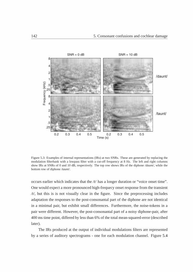
i

i

“MainFile” — 2010/7/15 — 15:31 — page 142 — #162i

i

i

i

i

i


Fre

quency (

kH

z)

SNR = 0 dB

.25

.5

1

2

4

8

SNR = 10 dB

Time (s)0.2 0.3 0.4 0.5

.25

.5

1

2

4

8

0.2 0.3 0.4 0.5

/daunt/

/taunt/

Figure 5.3: Examples of internal representations (IRs) at two SNRs. These are generated by replacing themodulation filterbank with a lowpass filter with a cut-off frequency at 8 Hz. The left and right columnsshow IRs at SNRs of 0 and 10 dB, respectively. The top row showsIRs of the diphone/daunt/, while thebottom row of diphone/taunt/.

occurs earlier which indicates that the/t/ has a longer duration or “voice onset time”.

One would expect a more pronounced high-frequecy onset response from the transient

/t/, but this is is not visually clear in the figure. Since the preprocessing includes

adaptation the responses to the post-consonantal part of the diphone are not identical

in a minimal pair, but exhibit small differences. Furthermore, the noise-tokens in a

pair were different. However, the post-consonantal part ofa noisy diphone-pair, after

400 ms time point, differed by less than 6% of the total mean-squared-error (described

later).

The IRs produced at the output of individual modulations filters are represented

by a series of auditory spectrograms - one for each modulation channel. Figure5.4

i

i

“MainFile” — 2010/7/15 — 15:31 — page 143 — #163i

i

i

i

i

i


shows these IRs for the diphone pair/daunt/ - /taunt/at a SNR of 10 dB. The first

channel is a lowpass filter which contains the “direct-current“(DC) energy of the

signal after auditory processing. In the other five channels, it can be observed that

for /daunt/ (left column), the strongest response has a shorter duration compared to

/taunt/, while the excitation amplitude is higher (darker color). The high modulation

frequency channels thus also contributed to a detection of differences in the diphone

pairs within the model.

Figure 5.5 shows IRs that reflect hypothetical hearing losses assumed in the

model. Consequences of broader auditory filters, IHC loss and a combination of the

two are illustrated. In order to isolate the effects, the IRswere generated using a linear

BM stage, the gammatone filterbank, which was also used in an earlier version of

the processing model (Dauet al., 1997a). The IR of /daunt/ produced by this model

(without the modulation filterbank) is shown in the upper left panel. To simulate

IHC loss, a constant attenuation of 25 dB was applied at the hair-cell stage across

frequencies. The corresponding IR is shown in the upper right panel. Consequently,

the amplitude of the response is reduced in the entire IR, butthe spectral resolution

is unchanged. To simulate broader filters, the bandwidths ofthe gammatone filters

were increased by a factor of 2 in all channels, resulting in the IR shown in the lower

left panel. As a consequence, the excitation is smeared across frequency and signal

information is reduced due to less resolved spectral components. A combination

of broader filters and IHC loss is presented in the lower-right panel. Here, it can

be observed that the amount of information is strongly reduced. The CASP model

fitted to the three individual listeners (described furtherbelow, Fig.5.10) provides

IRs reflecting individual level- and frequency-dependent combinations of reduced

sensitivity and reduced spectral and temporal resolution.

5.3.4 The back end

Messinget al. (2009) introduced the concept of using synthesized DRT diphones and

a detector (back end) based on theL2-norm. With their method, it can be assumed that

the source of model errors must be originating from the front-end processing. Here,

the same synthesized diphones and the same detector were used. Templates (Y ) were

the IRs of each diphone presented in a random realization of the noise, at a SNR of 5

i

i

“MainFile” — 2010/7/15 — 15:31 — page 144 — #164i

i

i

i

i

i


/daunt/

.512

4

.512

4

Fre

qu

en

cy (

kH

z)

.512

4

.512

4

.512

4

Time (s)

0.2 0.3 0.4 0.5

.512

4

/taunt/

0.2 0.3 0.4 0.5

0 Hz

5 Hz

10 Hz

17 Hz

28 Hz

46 Hz

Figure 5.4: Examples of IRs in the six modulation channels tuned to modulations center frequencies at 0, 5,10, 17, 28 and 43 Hz (top to bottom). The left column shows responses to/daunt/, while the right columnshows the responses to/taunt/. The SNR was 10 dB.

i

i

“MainFile” — 2010/7/15 — 15:31 — page 145 — #165i

i

i

i

i

i


Fre

quen

cy (

Hz)

Gammatone, normal tuning

.25

.5

1

2

4

8IHC loss (25 dB)

Time (s)

Broader filters (2x)

0.2 0.3 0.4 0.5

.25

.5

1

2

4

8IHC loss and broader filters

0.2 0.3 0.4 0.5

Figure 5.5: Examples of IRs to illustrate front-end processing consequences of simulated hearing loss.They were generated using a lowpass filter instead of the modulation filterbank, as in Fig.5.3. The upperleft panel shows the IR from/daunt/using the gammatone filterbank as the BM stage. The upper right panelshows the effect of a constant IHC loss of 25 dB. The lower leftshows the consequence of using broadergammatone filter, where the ERBs are doubled in all channels. The lower right panel exemplifies a responsewith both constant IHC loss and broader filters.

dB. For a given test diphone, the IR was calculated at a particular SNR (IRx), and the

mean-squared-errors (MSEs) between IRx and the two possible templates (e.g., for

/daunt/and/taunt/) was calculated across time, frequency and modulation frequency.

The MSE represents theL2-norm or Euclidean distance and is considered here as

representing theperceptualdistance between test IR and template. The MSE between

i

i

“MainFile” — 2010/7/15 — 15:31 — page 146 — #166i

i

i

i

i

i


IRx and the correct template (YC) was denoted MSEC , while the MSE calculated for

the corresponding wrong template (YW ) was denoted MSEW :

MSEC(x) =

∑NT

t=1

∑NF

f=1

∑NMF

mf=1[YC(t, f,mf) − IRx(t, f,mf)]2

NT NF NMF

(5.1)

MSEW (x) =

∑NT

t=1

∑NF

f=1

∑NMF

mf=1[YW (t, f,mf) − IRx(t, f,mf)]2

NT NF NMF

(5.2)

wherebyt represents the time index,f is frequency index andmf is the modulation

frequency index.NT , NF andNMF represent the total number of time, frequency

and modulation frequency indices, respectively. The argument x indicates that this

calculation is carried out for each of the 192 diphones. Detection is based on the

difference,∆MSE = MSEW − MSEC . Messinget al. used ahard decision

criterion, where the detector chooses the template which produces the smallest MSE as

representing the detected diphone. For∆MSE < 0, a wrong decision was made, while

for ∆MSE > 0, the correct word was detected. In the present study, a probabilistic

decision criterion was introduced which reflects the introduction of internal noise in

the model. In a binary task, the probability of being correctwhen∆MSE = 0 is 0.5.

In this new approach, the probability of being correct followed a Gaussian cumulative

density function (CDF) withµ = 0 and standard deviationσ, thus implying asoft

decision criterion.

CDF(x) =

∫ x

−∞

1√2πσ

exp(− x2

2σ2)dx (5.3)

To preserve the argumentation ofMessinget al.(2009) that the source of model errors

reflects front-end processing, it was important thatσ was fixed at this stage. Notice

that the introduced stochasticity in this detector, unlikethe back end in Messinget al.,

now introduce back-end errors. Therefore, predicted errorpatterns will be presented

as the mean error rates across 5 runs of the simulation.

Figure 5.6 shows examples of the∆MSE-distribution from actual simulations

using MNH, M1, M2 and M3. These show distributions produced while simulating

i

i

“MainFile” — 2010/7/15 — 15:31 — page 147 — #167i

i

i

i

i

i


the detection of voiced consonants (VC+) at the two tested SNRs. The distribution

produced by the MNH has most of the∆MSE-values greater than zero at the higher

SNR (10 dB), while there is an increased number of∆MSEs smaller than zero at 0

dB SNR. In the bottom panels, it can be seen that the HI models generally produce

narrower∆MSE-distributions but no increase in the occurrences of∆MSE < 0

relative to the NH model. Consequently, the HI models would not produce more

errors compared to the NH model if the hard decision rule was used. However, the

values of∆MSE are generally closer to zero in the HI models than in the NHmodel.

Thus, the use of the proposed probabilistic decision criterion will produce more errors

with the HI models.

i

i

“MainFile” — 2010/7/15 — 15:31 — page 148 — #168i

i

i

i

i

i


MNH

SNR = 10 dB

0

0.5

1MNH

SNR = 0 dB

0 200 400

M1

0 200 4000

0.5

1 M1

P(c

orre

ct)

0 200 400

M2

0 200 4000

0.5

1 M2

0 200 400

M3

0 200 4000

0.5

1 M3

∆ MSE

Figure 5.6: Example of∆MSE-distributions (gray bars in histograms) from the four models (MNH, M1,M2 and M3). These are produced from simulations of the VC+ dimension. Left and right columns showdistributions from 0 and 10 dB, respectively. The vertical dashed line indicates the decision boundary at∆MSE = 0, where the probability of being correct, P(correct), was 50%. The solid curve shows the CDFwhich determines P(correct) for detection as a function of∆MSE. σ of the CDF was constant at 25 in allmodels.

i

i

“MainFile” — 2010/7/15 — 15:31 — page 149 — #169i

i

i

i

i

i

5.4 Results 149

5.4 Results

5.4.1 Characterizing individual hearing impairment using non-

speech stimuli

Estimated BM input-output functions

The results from the TMC experiment are shown in Fig.5.7. The left and right

columns show the results at 1 and 4 kHz, respectively. The circles represent the

measured data obtained in the on-frequency masking condition. The open squares

show corresponding data obtained in the off-frequency condition. The horizontal

dashed lines indicate the thresholds for the signal withoutany masker. The error bars,

indicating± one standard deviation, are typically smaller than the datasymbol.

The off-frequency thresholds (squares) lie above the on-frequency thresholds

(circles), since an off-frequency masker produces less masking than an on-frequency

masker at the signal frequency. No data were obtained using the off-frequency masker

for S2 at the 4-kHz condition, since the necessary masker levels exceeded the limit

of the hardware (95 dB SPL). In order to be able to derive the BMI/O function in

this condition, the off-frequency TMC at 600 Hz, indicated by the asterisks, was used.

For listener S2 at 1 and 4 kHz, and S3 at 4 kHz the slope of parts of the on-frequency

TMC is steeper than the off-frequency TMC. This indicates BMcompression, and was

also observed, e.g., inNelsonet al. (2001) andJepsen and Dau(2010). In the case

of S1 at 1 kHz, the on- and off-frequency TMCs are roughly parallel which indicates

no BM compression, i.e. linear processing. However, for S1 at 4 kHz and S3 at 1

kHz, it can be observed that the slope of the on-frequency TMCis shallower than

that of the off-frequency TMC. This is not a typical result ofthis experiment, which

has been conducted in several studies using HI listeners. Here, it is assumed that BM

processing cannot be expansive, and these data may reflect inappropriate assumptions,

for these HI listeners, in the TMC method.

BM I/O functions were derived from the TMC data following theprocedure

suggested byNelsonet al. (2001). No data were obtained using the off-frequency

masker for S2 at the 4-kHz condition, since the necessary masker levels exceeded the

limit of the hardware (95 dB SPL). In order to be able to derivethe BM I/O function

i

i

“MainFile” — 2010/7/15 — 15:31 — page 150 — #170i

i

i

i

i

i


0

30

60

90S1

1 kHz

S1

4 kHz

0

30

60

90S2

Mas

ker

leve

l at t

hres

hold

(dB

SP

L)

S2

0 25 50 75 1000

30

60

90S3

0 25 50 75 100

S3



Figure 5.7: Results of the TMC experiment for the HI listeners. The left and right columns show resultswhere the signal frequency was 1 or 4 kHz, respectively. Opencircle and square symbols indicate thresholdsin the on- and off-frequency masking conditions, respectively. Error bars of one SD are generally smallerthan the symbol.

in this condition, the off-frequency TMC at 600 Hz was used. The circles in Fig.5.8

represent estimated I/O functions for the three listeners.These were obtained by using

a method similar toJepsen and Dau(2010): A straight line was in each case fitted to

the off-frequency masking data, which reflects the masker level at signal threshold as

a function of the masker-signal separation. These output levels were then plotted as

a function of the input level corresponding to the masker-signal intervals measured

i

i

“MainFile” — 2010/7/15 — 15:31 — page 151 — #171i

i

i

i

i

i

5.4 Results 151

with on-frequency masking. The dotted line has a slope of oneindicating a linear I/O

behavior.

40

60

80

100

1 kHz

S1

4 kHz

S1

40

60

80

100 S2

Out

put l

evel

(dB

)

S2

0 20 40 60 80 100

40

60

80

100 S3

0 20 40 60 80 100

S3


DRNL I/O NH

DRNL I/O HI

BM I/O

Figure 5.8: Measured and simulated BM I/O functions for the three HI listeners. Left and right columnsshow the results at 1 and 4 kHz, respectively. The circles indicate the measured I/O functions for listeners.The dashed curve shows the I/O function for the corresponding DRNL filter for MNH. The black curveindicates the DRNL I/O function adjusted to fit the measured I/O function. The dotted line indicates linearI/O behavior.

The slopes of the estimated I/O function were calculated andare shown in

Table 5.2. BM compression was found for listeners S2 at both 1 and 4 kHz,and

for S3 at 4 kHz, but in all cases slopes were higher than in NH listeners, i.e. above

i

i

“MainFile” — 2010/7/15 — 15:31 — page 152 — #172i

i

i

i

i

i


about 0.25. The three other conditions showed a slight expansion (S1 at 1 kHz) or a

substantial expansion (S1 at 4 kHz and S3 at 1 kHz). Indication of expansion is not

a typical result of this experiment, which has been conducted in several studies using

HI listeners. Here, it is assumed that BM processing cannot be expansive, and these

data may reflect inappropriate assumptions, for these HI listeners, in the TMC method.

However, some studies reported a few listeners were the slopes were higher than one

(up to 1.70 inRosengardet al. (2005) and up to 1.56 inStainsby and Moore(2006)).

It remains unclear why substantial expansion was observed.It was not possible to

determine a knee point in any of the estimated I/O functions here. As inJepsen

and Dau(2010), the general observation was that I/O functions were different across

listeners even though their sensitivity at the tested frequencies was comparable..

Listener S1 S2 S3BM compression, 1 kHz 1.34 0.36 2.88BM compression, 4 kHz 2.01 0.66 0.64

Table 5.2: Estimated BM compression exponents in units of dB/dB

Simulated BM I/O functions, sensitivity and frequency tuning

The dashed curve in Fig.5.7shows the DRNL model’s I/O function for normal hearing

at the corresponding signal frequencies. Following the procedure suggested inJepsen

and Dau(2010), a set of frequency-dependent DRNL parameters (a, b, c andg) was

determined, such that the DRNL I/O function fitted the BM I/O data. In the three cases

where the estimated compression exponent was higher than one (expansive). There are

no psychophysical or physiological data on the literature that suggest expansive BM

I/O behavior, so when the present data suggest expansion, the model processing was

assumed to be linear. The solid black curves represent the fitted DRNL I/O functions.

The sensitivity loss due to OHC loss (HLOHC) was estimated on the basis of these

derived DRNL I/O functions for 0.25, 0.5, 1, 2, 4 and 8 kHz. Thevalues of HLOHC

for the three listeners at 1 and 4 kHz, and the range of estimated HLOHC over all

frequencies are listed in Table5.3. Values of HLOHC of ranged from 10 dB to 45 dB.

Less compression was reflected by higher values. The IHC losscomponent (HLIHC)

i

i

“MainFile” — 2010/7/15 — 15:31 — page 153 — #173i

i

i

i

i

i

5.4 Results 153

was assumed to represent the difference between the total sensitivity loss reflected in

the audiogram (HLTOT) and HLOHC, i.e., HLIHC = HLTOT − HLOHC. The results for

each listener at 1 and 4 kHz as well as the range over all frequencies are listed in

Table5.3. The HLIHC estimates are in the range from 0 to 35 dB. Overall, the data

suggest that S1 and S3 primarily had lost sensitivity due to OHC loss, while for S2 the

sensitivity loss appears distributed equally between OHC and IHC loss. The models

fitted to listeners S1, S2 and S3 were named M1, M2 and M3. Pure-tone thresholds

were predicted and are indicated by the black symbols in Fig.5.1. It can be seen that

the frequency dependent sensitivity is appropriately accounted for, typically within

10 dB. This was expected since the audiogram was used to determine the value for

HLIHC.

Listener S1 S2 S3HLOHC at 1 kHz (dB) 35 25 35HLOHC at 4 kHz (dB) 45 35 35HLOHC range in filterbank 17-45 10-35 10-45HLIHC at 1 kHz (dB) 10 20 0HLIHC at 4 kHz (dB) 10 10 10HLIHC range in filterbank 0-15 10-35 0-10

Table 5.3: Estimated loss of sensitivity due to OHC and IHC loss in dB. HLOHC-values were obtainedfrom the model’s individually fitted I/O function. HLIHC was estimated from the value of HLOHC and theaudiogram

Further individual differences were explored by investigating the tuning of the

DRNL filters of M1, M2 and M3. The tuning of the filters was represented by iso-

intensity response functions in Fig.5.9. They are shown for four center frequencies

(at 0.5, 1, 2 and 4 kHz) and at two different input levels, 30 (dashed) and 70 dB SPL

(solid). Such simulated filter tuning was shown to resemble roex filters measured

in individual listeners inJepsen and Dau(2010). The top panel shows the level-

dependent DRNL tuning for MNH. The lower input level produced the most sharply

tuned response curves. This is a direct consequence of the compression in the model.

The filterbank of M1 had completely linear BM processing; thefilters were generally

broader and had no dependency on level. The DRNL filters of M2 had residual

compression. The tuning was thus close to that of the NH modelfor the highest

i

i

“MainFile” — 2010/7/15 — 15:31 — page 154 — #174i

i

i

i

i

i


level and level-dependency could only be seen at 2 and 4 kHz (at the levels tested

here). The filters of M3 were broad and level-independent at 0.5 and 1 kHz, while

their relative sharpness increased for the higher center frequencies. Level-dependent

tuning was only observed at 4 kHz.

−40

−20

0 MNH

−40

−20

0 M1

DR

NL

outp

ut (

dB, r

e m

ax)

−40

−20

0 M2

0.25 0.5 1 2 4 8−40

−20

0 M3

Frequency (kHz)

Figure 5.9: Simulated BM tuning for the four models (MNH, M1, M2and M3). The iso-intensity responsefunctions for DRNL filters are shown for center-frequenciesat 0.5, 1, 2 and 4 kHz. The dashed curves wereproduced from an input level of 30 dB SPL and the solid line from 70 dB SPL. The tip gains are normalizedto the corresponding max filter gains.

i

i

“MainFile” — 2010/7/15 — 15:31 — page 155 — #175i

i

i

i

i

i

5.4 Results 155

Simulated internal representations of speech sounds

Figure 5.10 illustrates how the simulated individual BM compression, frequency

selectivity and IHC loss affected the processing of the speech signals in the framework

of the model. The shown IRs of MNH and three HI models were generated from

/daunt/ at a SNR of 10 dB, in a manner similar to those of Fig.5.5, but here using

the individually fitted processing. The IR of MNH is identical to the upper right panel

of Fig. 5.3, and was re-plotted here for a better visual comparison. In the IR of M1

it can be observed that the corresponding signal was less resolved in frequency, and

the overall amplitude of excitation is reduced (brighter colors). This was expected due

to the linear BM processing, and consequently lower sensitivity. For M2 it is clear

that most low-frequency (< 500 Hz) information is lost due tothe reduced sensitivity

in these channels. The frequency resolution for the mid- andhigh frequencies was

higher than for M1. This reflected the simulated residual compression M2. M3 show a

stronger excitation compared to M1 and M2, since listener S3had the mildest hearing

loss in terms of sensitivity. The frequency resolution is reduced at least at frequencies

below 1 kHz, as expected from Fig.5.9.

5.4.2 DRT error patterns

Measured error patterns

The human performance in the DRT is presented as the error rate percentage in each

of the tested acoustic-phonetic dimensions; VC, NS, ST, SB,GV and CM. They are

further resolved in two groups, indicating whether the attribute was present (+) or not

(−). The chance level in this task was 50% and is indicated by thedashed horizontal

line. The error rates are shown in Fig.5.11 for the NH listeners and the three HI

listeners, represented by the bars. These plots are referred to as DRT error patterns.

These error rates also represent the target rates for the model predictions. The data

for NH listeners were taken fromMessinget al. (2009) at the corresponding signal

level and SNR (their Fig. 9, panels "70dB SPL 0 dB SNR" and "60dB SPL 10 dB

SNR"). They represent mean errors of 6 NH listeners, and the error bars indicate±one standard deviation (SD) across listeners. For the NH listeners, it can be observed

that the dimensions VC−, ST+ and ST− have the highest error rates. The remaining

i

i

“MainFile” — 2010/7/15 — 15:31 — page 156 — #176i

i

i

i

i

i

156 5. Consonant confusions and cochlear damageF

requ

ency

(kH

z)

MNH

.25.5

1

2

4

8

.25M1

Time (s)

M2

0 0.1 0.2 0.3 0.4.25.5

1

2

4

8

.25M3

0 0.1 0.2 0.3 0.4

Figure 5.10: Examples of IRs of the four models (MNH, M1, M2 and M3). They were generated fromdiphone/daunt/at an SNR of 10 dB.

dimensions typically have error rates below 20% and for NS the error rate is close to

zero errors. The general trend was that more errors were produced at the lower SNR (0

dB). According toMessinget al.(2009) these error rates are similar to those produced

with natural DRT stimuli.

The remaining data were obtained by the three HI listeners ofthe present study.

Here, the error bars indicate± one SD across eight diphone repetitions within the

listener. Listener S1 clearly produced more errors than theNH listeners at both

SNRs. ST+ has the highest amount of errors of about 60%, exceeding chance level.

i

i

“MainFile” — 2010/7/15 — 15:31 — page 157 — #177i

i

i

i

i

i

5.4 Results 157

0

20

40

60

SNR = 0 dB

NH

SNR = 10 dB

NH

0

20

40

60

Err

or r

ate

(%)

S1 S1

0

20

40

60 S2 S2

+− +− +− +− +− +−0

20

40

60

VC NS ST SB GV CM

S3

+− +− +− +− +− +−VC NS ST SB GV CM

S3

Figure 5.11: Measured error patterns of the DRT at the two SNRs (0 and 10 dB). The bars indicate the errorrate in percent in the six acoustic-phonetic dimensions, and+/− indicate if the attribute was present or not.The data in the top row (NH) is re-plotted fromMessinget al. (2009) in the SNR conditions correspondingto those of the present study. The three remaining rows show data measured in the three HI listeners of thepresent study. Error bars indicate±one SD. The horizontal dashed line indicates the chance level at 50%.

For the dimensions VC, SB, GV and CM the amount of errors were about twice

of that obtained in the NH listeners or higher. However, thislistener showed good

i

i

“MainFile” — 2010/7/15 — 15:31 — page 158 — #178i

i

i

i

i

i


performance in the NS condition. Overall, slightly fewer errors were found at the

higher SNR (10 dB). S1 had the worst overall performance among the HI listeners of

this study. S2 showed a high error rate (above 30%) in all dimensions at 0 dB SNR,

except for NS. At SNR = 10 dB there a substantially fewer errors, so it seems that S2

had a great benefit from the better SNR (except for dimension ST). Interestingly, S2

was the only HI listener producing errors in dimension NS higher than 6%. S3 also

shows a benefit from the better SNR, and had the best performance at SNR = 0 dB

among the HI listeners.

Simulated error patterns

The predicted error patterns of the models simulating normal hearing (MNH) and

individual hearing loss (M1, M2 and M3) are shown in Fig.5.12. The error bars

indicate± one SD across three model runs of the DRT. The error rates had aslight

variability across runs, since a stochastic decision criterion was used. The SDs were

typically within 4%. For MNH at SNR = 0 dB it can be seen that error rates for

VC, ST, SB and CM were about 20%. For GV they were about 28%, andfor NS

the error rates were close to zero. At SNR = 10 dB there were generally about 10%

fewer errors with a similar error pattern. Model M1 producedmore errors than MNH.

At SNR = 0 dB there were about 5-10% more errors for ST, SB and CM, while the

other dimensions, VC, NS and GV, had about the same error rateas for MNH. This

may indicate that the discrimination cues used in ST, SB and CM are less robust to

noise due to supra-thresholds deficits. At SNR = 10 dB there were generally 2-13%

more errors than MNH, except for NS where both MNH and M1 produce zero errors.

There were slightly fewer errors at the higher SNR. For M2 at SNR = 0 dB there was

generally about 20% errors, except for dimension GV which had 32 and 34% errors.

At SNR = 10 dB there were fewer errors (up to 11%), especially for NS, SB and GV.

M2 was the only model that produced a substantial amount of errors in dimension NS.

Model M3 generally had a very low error rates of about 10 to 23%at SNR = 0 dB

and 4 to 20% and SNR = 10 dB. In dimension NS there were virtually zero errors.

Errors rates were mostly lower than those produced by MNH at both SNRs, which

was unexpected. It is unclear whether this reflect unrealistic simulation of degraded

i

i

“MainFile” — 2010/7/15 — 15:31 — page 159 — #179i

i

i

i

i

i

5.4 Results 159

auditory processing, or if the back end needs to be modified toappropriately handle

the template matching after degraded auditory processing.

0

20

40

60

SNR = 0 dB

MNH

SNR = 10 dB

MNH

0

20

40

60

Err

or r

ate

(%)

M1 M1

0

20

40

60 M2 M2

+− +− +− +− +− +−0

20

40

60

VC NS ST SB GV CM

M3

+− +− +− +− +− +−VC NS ST SB GV CM

M3

Figure 5.12: Error patterns predicted by the four models (MNH, M1, M2 and M3), corresponding toFig. 5.11.

i

i

“MainFile” — 2010/7/15 — 15:31 — page 160 — #180i

i

i

i

i

i


Comparison between human and model error patterns

The target error rates of the models were the individual human error rates. Aχ2-

statistic was used to evaluate if the match between model andhuman error rate was

significant. This metric was also used inMessinget al. (2009). It evaluates whether

error rates were statistically similar or different. Lowervalues of theχ2-statistic reflect

closer matches. If theχ2-value is lower than a critical value it cannot be rejected that

the errors rates are the same. For one degree of freedom thesecritical value is 3.84 at

confidence level of 95%. Here matches within the 95% level were considered good.

Figure5.13shows theχ2-values in for the acoustic-phonetic features. Formally these

values can only be positive, but here a sign has been added to indicate whether errors

were over- or underestimated. Negative values reflect that the model produced too

few errors. The critical value is indicated by the horizontal gray lines. The bars were

colored black if the values exceeded the critical value. Forthe two SNR conditions

the MNH model produce close matches in most of the acoustic-phonetic dimensions.

At the lower SNR (0 dB) for GV- the error were substantially overestimated. For the

models simulating hearing imapairment different trends appear. For model M1 the

matches are genrerally fair, except for the ST+ dimesnion were the amount of errors

were substantially underestimated. This was also the case for the simulated errors

by model M3. Model M2 oervall produced a good match at the lower SNR, but at

the higher SNR the model generally produced too many errors.The meanχ2-values

(without sign change) for the individual listeners at the two tested SNRs are shown in

Table5.4. If the meanχ2-value was lower than the critical value (3.84) the simulated

error pattern was considered a fair overall match to the data. The mean critical value

was lower than the critical value in six of the eight conditions. The two conditions

were there was a significant difference was for M2 in the 10-dBSNR condition and

for model M3 in the 0-dB SNR condition.

SNR (dB) MNH− NH M1 − S1 M2− S2 M3− S30 3.82 3.78 3.01 6.7410 2.09 2.52 7.72 3.76

Table 5.4: χ2-values between measured and predicted error patterns, averaged across acoustic-phoneticfeatures in the DRT.

i

i

“MainFile” — 2010/7/15 — 15:31 — page 161 — #181i

i

i

i

i

i

5.4 Results 161

Error patterns due to reduced sensitivity alone

The error patterns from by the models that only simulate reduced sensitivity (A1,

A2 and A3) are compared to those simulating hearing loss due to loss of hair-cells

leading to reduced sinsetivity and suprathreshold deficits. In Fig. 5.14error patterns

are compared in terms of the error rate difference in percentage points (pp). Zero

error rate differences represent perfect matches. Negative bars indicate that simulated

supra-threshold deficits contribute to a larger number of errors in the DRT - up to 20%

in several cases. For the models simulating the peripheral processing of listener S1 and

S2, it is clear that the supra-threhold deficits have a large influence, whereas for models

A3 and M3 produce similar amounts of errors. The simulationsfrom the "sensitivity-

only" model are compared to the human data in theχ2 sense and the values are shown

in Table5.5. In none of the conditions the meanχ2-value falls within the critical limit

at 3.84. Thus, the relatively fewer errors produced by the "sensitivity-only" models

generally led to unreasonable macthes to the human data. Theχ2-analysis was also

used to test whether the error patterns of the two models, simulating each listener, was

significantly different (bottom rows of Table5.5). Significant differences were found

in only two of the six conditions (A1/M1 at 10-dB SNR and A2/M2at 10-dB SNR).

SNR (dB) A1− S1 A2− S2 A3− S30 5.60 5.34 6.7910 7.26 4.53 6.85

SNR (dB) A1− M1 A2 − M2 A3 − M30 1.80 2.02 0.5310 4.19 7.22 0.69

Table 5.5: χ2-values calculated to evaluate the matches between the "sensitivity-only" models and thehuman data (top rows), and comparing the two model configurations for the individual listeners (bottomrows)

i

i

“MainFile” — 2010/7/15 — 15:31 — page 162 — #182i

i

i

i

i

i


−40

−20

0

20

SNR = 0 dB

MNH − NH MNH − NH

SNR = 10 dB

−40

−20

0

20

χ2 val

ue

M1 − S1 M1 − S1

−40

−20

0

20M2 − S2 M2 − S2

+− +− +− +− +− +−−40

−20

0

20

VC NS ST SB GV CM

M3 − S3

+− +− +− +− +− +−VC NS ST SB GV CM

M3 − S3

Figure 5.13: The match of predicted and human error rates in terms of χ2-statistics. Gray bars indicatecases where the value is lower than the critical value (3.84). Black bars indicate cases where the criticalvalue is exceeded. Negative bars reflect that errors are underestimated by the model.

i

i

“MainFile” — 2010/7/15 — 15:31 — page 163 — #183i

i

i

i

i

i

5.4 Results 163

−40

−20

0

20

Err

or r

ate

diffe

renc

e (p

p)

A1 − M1 A1 − M1

−40

−20

0

20A2 − M2 A2 − M2

+− +− +− +− +− +−−40

−20

0

20

VC NS ST SB GV CM

A3 − M3

+− +− +− +− +− +−VC NS ST SB GV CM

A3 − M3

Figure 5.14: Contribution from simulated supra-threshold deficits in terms of the error rate difference inpercentage points (pp). Negative bars indicate that simulated supra-treshold effects lead to more errors.

i

i

“MainFile” — 2010/7/15 — 15:31 — page 164 — #184i

i

i

i

i

i


5.5 Discussion

5.5.1 Front-end processing

The predicted error patterns were in reasonable agreement with the measured error

patterns, except for a few particular acoustic-phonetic dimensions. This indicates

that the front-end processing, which was fitted to the hearing loss of the individual

listeners, appropriately simulates internal representations in the hearing-impaired

listeners. However, errors rates were systematically underestimated in three particular

acoustic-phonetic dimensions. It is yet unclear if this discrepancy is due to

inappropriate front-end or back-end processing. Similar results were obtained for NH

listeners inGhitza(1993) andMessinget al. (2009). The result of this study is, to the

knowledge of the authors, the first time that a relation between speech and non-speech

data has been shown in listeners with cochlear hearing loss.The IR reflects aspects

of both sensitivity and supra-threshold deficits. The simulated supra-threshold effects

are consistent with the current understanding of consequences of cochlear damage,

that is, changes in frequency selectivity and temporal resolution. These effects are

crucial for describing the variability in results of HI listeners and can presumably

not be accounted for by using threshold shaped noise maskingof a model of normal

hearing (e.g.,Holube and Kollmeier, 1996). However, this was not explicitly tested

here.

The adaptation stage of the CASP model was crucial in order toaccount for,

among other aspects, temporal masking (Dauet al., 1996a, 1997a; Jepsenet al., 2008).

Such effects were not included in the front-end used inMessinget al.(2009). Another

effect of adaptation was logarithmic compression for stationary inputs, e.g., for the

noise used in the present study. This reduced the dynamic range of the response to

the noise, and may be effectively similar to the concept of the dynamic range window

introduced inMessinget al. (2009), which they assigned to simulate efferent control.

No stages of efferent effects were considered in the CASP model. However, in terms

of the predicted DRT error patterns for NH listeners, the performance of the present

model and that of Messinget al. are comparable.

It was further found that the prediction using the modulation filterbank was better

than using an energy representation (e.g.,Dauet al., 1996a). Aspects of, e.g., onset

i

i

“MainFile” — 2010/7/15 — 15:31 — page 165 — #185i

i

i

i

i

i

5.5 Discussion 165

timing was represented in more detail using the modulation filters and adding up to

six modulation filters affected the pattern of errors.Jürgens and Brand(2009) used an

earlier version of the CASP model as front-end. They used thefirst four modulation

channels. It is unclear why they did not include filters tunedto higher modulations

rates. In other auditory models intended as front-ends for speech intelligibility, the

analysis was performed in time-frames.Messinget al.(2009) used temporal windows

of about 8-12 ms to find the short term average of the output. Jürgens and Brand

used down-sampling to get instantaneous output values at every 10 ms (100 Hz). In

the present study, the temporal sampling rate of the IRs was 1kHz, which means that

more temporal information, e.g. fine-structure, was preserved at frequencies up to 500

Hz which could be relevant for speech perception.

By using versions of the model that was fitted to the HI listeners, and simulating

only loss of sensitivity, it was explored how the simulationof supra-threshold deficits

affected the DRT error patterns. It was found, that for the predictions of the data for

two out of the three listeners, error rates were substantially underestimated. This

indicates that simulation of reduced spectral and temporalresolution does have a

considerable influence on the simulations relating to speech perception. InHolube

and Kollmeier(1996) they attempted similar explorations, but they did not find large

effects of simulating broader filters in their predictions of the data in their speech task.

However, they did not include realistic simulation of nonlinear cochlear processing in

their model.

5.5.2 Back-end processing

The underlying assumption in the detector was that the dominant source of errors

produced by the model was due to insufficient information to discriminate a diphone

pair, after front-end processing. The use of the synthesized DRT stimuli, combined

with the template matching paradigm, allowed this assumption. However, due to the

adaptation stage in the CASP model the IR depends on the previous samples over an

interval of 500 ms. However, it is likely that this side-effect does not influence the

predicted error rate, since major contributions to the calculated MSEs were within the

time-range of the initial consonant. The contribution fromthe last 200 ms of the IRs

to the∆MSEs was in the range from 0 to 6%.

i

i

“MainFile” — 2010/7/15 — 15:31 — page 166 — #186i

i

i

i

i

i


It remains unclear at which SNR the template should be generated. In previous

studies using the CASP model to predict masking and discrimination data, the SNR of

the template was usually at a high SNR compared to the expected detection threshold.

Here, a SNR of 5 dB, thus between the two tested SNRs (0 and 10 dB) was chosen,

similarly to Messinget al. (2009) who found this to be the optimal choice. This may

not necessarily be optimal using the CASP model as the front end.

Jürgens and Brand(2009) used perfecta priori knowledge of the stimuli to obtain

the best matches to human performance, that is, templates were derived from signals

identical to the test stimuli. They used naturally uttered nonsense logatoms. In order to

account for the variations in the stimuli they used a dynamictime-warp stage in their

detector. This stage may introduce some errors, due to time-compression or expansion

and it is not possible to separate if predicted confusion errors are due to this stage or

the front-end. Also, information about timing differences, which may aid detection,

was lost in the dynamic time-warp stage. Timing cues are of great importance in

discriminating consonants (e.g.,Régnier and Allen, 2008).

5.5.3 Limitations of the approach

The results obtained here with synthesized stimuli are useful, since front end and back

end were clearly separated. The experimental data do not reflect aspect of natural

variations of uttered diphones. These variations depend on, e.g., speaker differences,

co-articulation etc. The current detector cannot account for these variations in time

and frequency. Future studies should address this issue.

Here, templates were derived from signals embedded in noise. If it is assumed

that human observers have stored templates of speech sounds, they may be "clean"

or there may be several templates representing a broad rangeof speech sounds at

different SNRs. It is also a question whether hearing-impaired listeners have templates

reflecting a normally functioning periphery, or if they adjust templates over time due to

their degraded representations (neural plasticity). The listeners here had hearing losses

since early childhood, and templates were derived from their individual impaired

auditory processing.

The error rates of the VC−, ST+ and ST− dimensions were substantially

underestimated. This was also a general problem in the modelpredictions of

i

i

“MainFile” — 2010/7/15 — 15:31 — page 167 — #187i

i

i

i

i

i

5.5 Discussion 167

Messinget al. (2009). These are also the conditions where the NH listeners showed

substantially worse performance in the DRT using syntheticdiphones, compared to

natural diphones (Messinget al., 2009). The missing capability to predict these error

rates may reflect that the detector of the present model is toosensitive to timing cues.

Voicing and sustention are the features which primarily depend on timing-differences

in a minimal pair, while the remaining features depend more on spectral or spectro-

temporal differences. It is unclear if the human observers can use a timing precision

of about 1 ms in their decision, although the information maybe available in the

peripheral representation.

i

i

“MainFile” — 2010/7/15 — 15:31 — page 168 — #188i

i

i

i

i

i


5.6 Conclusions

• Cochlear hearing loss in three individual listeners were characterized due

to their audiograms and estimated basilar-membrane I/O functions. The

parameters of the cochlear stage of the CASP model were fittedto these data.

The model was then used as a front end in a speech detector system.

• The model with individualized front-ends could predict most aspects of DRT

error patterns measured in the same listeners, except for a few particular

conditions were DRT error rates are substantially underestimated by the model.

Since the modeling framework could separate front-end and back-end errors, the

capability of the model to predict the error patterns shows that there is a relation

between the limited auditory function, characterized on the basis of non-speech

data, and speech perception.

• There were considerable differences between the predictederror patterns by

the suggested model and a model that was designed to only simulate reduced

sensitivity in the individuals.

• The suggested framework, combining the CASP front end with the back end

based on synthetic DRT stimuli, might be interesting in applications, e.g., to

objectively assess the perceptual implications of signal processing algorithms

of hearing aids in HI listeners.

i

i

“MainFile” — 2010/7/15 — 15:31 — page 169 — #189i

i

i

i

i

i

6General discussion

In this thesis, a model was proposed that simulates auditorysignal processing and

perception. This model was first developed to simulate the normally functioning

auditory system. The focus was to include a realistic cochlear processing stage into

an existing modeling framework that assumed linear processing at this stage. Second,

it was shown how consequences of individual cochlear hearing impairment can be

characterized experimentally and accounted for by the model. Third, the peripheral

part of the model was used as a front-end in a speech recognizer designed for

consonant discrimination. It was shown that the model usingindividually fitted front-

end parameters can account for many characteristics of the individual error patterns in

the data from hearing-impaired (HI) listeners.

The computational auditory signal-processing and perception (CASP) model

was shown to account for various data from psychoacoustic detection and masking

experiments (Chapter2). The inclusion of the nonlinear basilar-membrane (BM)

stage increased the predictive power of the model, particularly in conditions where

the results are affected by the level-dependent cochlear processing, such as spectral-

masking patterns and forward masking. This was an importantresult since previous

studies had raised concerns about the combination of the compressive cochlear stage

and the subsequent adaptation stage assumed in the model framework (Derleth et

al., 2001). Here, it was shown that there was no principal limitation in combining

the two stages; however, it was necessary to include a stage of level-independent

expansion to account for the data in the tested experimentalconditions, particularly

in forward masking. Another key finding was that intensity discrimination data could

be accounted for. The question was whether the compressive properties of the BM

stage would results in an underestimation of intensity JNDs. However, intensity

discrimination data were accurately accounted for, since the linear off-frequency

169

i

i

“MainFile” — 2010/7/15 — 15:31 — page 170 — #190i

i

i

i

i

i

170 6. General discussion

processing in neighboring channels of the cochlear filterbank model dominates the

processing in this task within the model, since off-frequency channels realize a

logarithmic compression. This results in JNDs of approximately 1 dB. The model

was further modified in the modulation processing stage, where the sensitivity to

high modulation rates (above 150 Hz) was reduced by a lowpassfilter prior to the

modulation filterbank stage. Here, it was shown that the model’s ability to account

for temporal modulation transfer functions in narrowband and wideband carriers was

preserved, at least for modulation rates at up to 250 Hz.

In Chapter 4, perceptual consequences of cochlear hearing loss including

sensitivity and supra-threshold limitations, were considered in individual listeners.

For ten HI listeners, an individual parameter-set for the cochlear stage of the CASP

model was derived, based on the experimental estimates of BMI/O functions and

the audiogram. Individual frequency-specific estimates ofthe effect of outer hair-

cell (OHC) and inner hair-cell (IHC) loss on sensitivity were obtained. One key

finding was that these estimates varied largely across listeners, and could not be

predicted based on the audiogram alone. Within the model, a reduced or lost BM

compression associated with OHC loss had direct consequences for BM tuning. It was

shown that the model could account for individual frequencyselectivity as measured

independently in all listeners, even though some systematic discrepancy was found at

one tested frequency. The model successfully accounted forthe individual thresholds

in simultaneous- and forward masking conditions. The results indicate that individual

BM I/O behavior combined with the audiogram provide sufficient information about

cochlear hearing loss to describe the tested supra-threshold effects.

The experimental characterization of BM I/O functions in Chapter 4 showed

that stable estimates of BM compression as well as the I/O-function knee point are

useful quantities in order to simulate individual cochlearhearing loss. Chapter3

described an attempt to extend the growth-of-masking (GOM)experiment (Oxenham

and Plack, 1997). It was shown that the knee point of the BM I/O function could

be accurately estimated with the modified paradigm in addition to estimating the

amount of BM compression. The results demonstrated that an estimate of the BM I/O

function could be estimated for a wider range of input levelsthan in the case of the

original method by using two different masker-signal interval conditions. The within-

i

i

“MainFile” — 2010/7/15 — 15:31 — page 171 — #191i

i

i

i

i

i

171

listener variability in the data was small compared to that found previously in the

alternative temporal masking curve (TMC) method (Nelsonet al., 2001; Rosengard

et al., 2005). The extended GOM method thus represents a method of estimating

BM I/O-functions which produces robust data. However, the capability to accurately

estimate knee point depends on the appropriate choice of masker-signal interval in

a particular experimental condition. For NH listeners, theknee point estimate was

obtained with a constant masker-signal interval. For HI listeners, however, the choice

of masker-signal interval should be chosen individually for measured ears, based on

pilot experiments. The suggested method could have been used to obtain the BM

I/O functions in Chapter4, but it was decided to use the established and commonly

used TMC method (Nelsonet al., 2001), since it was not yet explicitly shown if more

stable results could be obtained in HI listeners with the newmethod. Furthermore the

method of Chapter3 required more testing time compared to the TMC method.

The results reported in Chapter5 showed that consonant discrimination error

patterns were mostly accounted for using auditory processing front-end that had been

fitted to individual cochlear hearing loss. The model’s back-end and the synthetic

speech stimuli were designed such that front-end and back-end errors were separated.

Otherwise it would not have been possible to assign consonant discrimination

error patterns to the degraded auditory processing in the models describing hearing

loss. The results indicated that it is possible to use a modelof detailed auditory

preprocessing as a front-end in an speech intelligibility application. The results further

indicated that there is a relation between the performancesof individual HI listeners

in speech versus non-speech perception tasks. However, forthree particular acoustic-

phonetic feature dimensions the errors were substantiallyunderestimated both for

MNH and the three model of hearing impairment. It is still unclear exactly why

this is the case, but the back end of the model may be too sensitive to timing cues

which are important in these partilar dimensions. The current findings support that

supra-thresholds consequences of cochlear damage are crucial to speech perception,

and that audibility alone cannot be expected to explain degraded speech perception

in HI listeners. In future studies, back-ends which can handle natural speech stimuli

(instead of the synthesized stimuli considered here) may lead to models that account

for data in a broader selection of speech materials.

i

i

“MainFile” — 2010/7/15 — 15:31 — page 172 — #192i

i

i

i

i

i

172 6. General discussion

The modeling framework suggested in this thesis may be interesting and useful

for applications, such as systems which objectively assessspeech intelligibility

or audio quality, as perceived by hearing-impaired listeners. For example, new

compensation strategies or signal-processing algorithmsin hearing aids (HA) could

be tested in a carefully designed system to give rough estimates of the outcome

of listening tests, which are otherwise expensive and time-consuming. A scheme

for the objective assessment of the effect of hearing-aid processing is suggested in

Fig. 6.1. Consider an assessment system where the model, with a back-end (such as

an optimal detector or speech recognizer), can account for some data (non-speech,

speech intelligibility, sound quality etc.) from both NH listeners and a HI listener.

If hearing-aid processing is introduced prior to the model representing the impaired

periphery of the HI listeners, the implications of the HA processing can be observed

at the output of the complete model. The outcome could then becompared to that of

the model of normal hearing. The HA processing could subsequently be adjusted

to match the performance of the NH model or to further reduce errors, e.g., in

consonant discrimination error patterns (see, e.g., Chapter 5). Subjective testing

cannot be expected to be completely replaced, but objectiveassessment tools may

provide useful estimates of the effects of distortions and improvements resulting from

the tested algorithms. Some of the experiments considered in this thesis to characterize

individual hearing loss are time-consuming. Thus, the suggested framework is

probably not applicable to HA fitting in individual patients. However, for research

and development purposes, the experiments presented here should not necessarily be

repeated, since the current modeling framework, includingthe results of this thesis,

already provides parameter-sets to describe a variety of HIlisteners. These may

comprise a representative sample of current or potential hearing-aid users.

Stimulus Front-end Back-end Output

Signal in noise

Speech in noise

CASP NH

CASP HI

Optimal detector

Speechrecognizer/detectorHearing

aid

Masked threshold

Speech discriminationerror pattern

Masked threshold

Speech discriminationerror pattern

compare

Figure 6.1: Example of a scheme to test perceptual implicationsof hearing-aid processing, using theauditory processing model framework suggested in this thesis

i

i

“MainFile” — 2010/7/15 — 15:31 — page 173 — #193i

i

i

i

i

i

References

ANSI (1969). “S3.5-1969: Methods for calculation of the articulationindex,”American National Standards Institute, New York .

ANSI (1997). “S3.5-1997: Methods for calculation of the speech intelligibility index,”American National Standards Institute, New York .

Bacon, S. P., and Gleitman, R. M. (1992). “Modulation detection in subjects withrelatively flat hearing losses,” J. Speech Hear. Res.35, 642– 653.

Bacon, S. P., and Grantham, D. W. (1989). “Modulation masking: Effects ofmodulation frequency, depth and phase,” J. Acoust. Soc. Am.85, 2575–2580.

Bacon, S. P., and Viemeister, N. F. (1985). “Temporal modulation transfer functionsin normal-hearing and hearing-impaired listeners,” Audiology 24, 117–134.

Borg, E., and Engström, B. (1989). “Noise level, inner hair cell damage, audiometricfeatures, and equal-energy hypothesis,” J. Acoust. Soc. Am. 86, 1776–1782.

Breebaart, J., van de Par, S., and Kohlrausch, A. (2001a). “Binaural processing modelbased on contralateral inhibition. I. Model structure.,” J. Acoust. Soc. Am.110,1074–1088.

Breebaart, J., van de Par, S., and Kohlrausch, A. (2001b). “Binaural processingmodel based on contralateral inhibition. II. Dependence onspectral parameters.,”J. Acoust. Soc. Am.110, 1089–1104.

Breebaart, J., van de Par, S., and Kohlrausch, A. (2001c). “Binaural processing modelbased on contralateral inhibition. III. Dependence on temporal parameters.,” J.Acoust. Soc. Am.110, 1105–1117.

Bruce, I. C., Sachs, M. B., and Young, E. D. (2003). “An auditory-periphery modelof the effects of acoustic trauma on auditory nerve responses,” J. Acoust. Soc. Am.113, 369–388.

173

i

i

“MainFile” — 2010/7/15 — 15:31 — page 174 — #194i

i

i

i

i

i

174 References

Buchholz, J. M., and Mourjoloulus, J. (2004a). “A computational auditorymasking model based on signal dependent compression. I. Model description andperformance analysis,” Acustica - Acta Acustica5, 873–886.

Buchholz, J. M., and Mourjoloulus, J. (2004b). “A computational auditory maskingmodel based on signal dependent compression. II. Model simulations and analyticalapproximations,” Acustica - Acta Acustica5, 887–900.

Burns, E. M., and Viemeister, N. F. (1981). “Played-again SAM: Further observationson the pitch of amplitude-modulated noise,” J. Acoust. Soc.Am. 70, 1655–1660.

Carlyon, R. P., and Shamma, S. (2003). “An account of monaural phase sensitivity,” J.Acoust. Soc. Am.114, 333–348.

Carney, L. H., Heinz, M. G., Evilsizer, M. E., Gilkey, R. H., and Colburn, H. S.(2002). “Auditory phase opponency: A temporal model for masked detection atlow frequencies,” Acta. Acust. Acust.88, 334–347.

Carney, L. H. (1993). “A model for the responses of low-frequency auditory-nervefibers in cat,” J. Acoust. Soc. Am.93, 401–417.

Chi, T., Gao, Y., Guyton, M. C., Ru, P., and Shamma, S. (1999). “Spectro-temporalmodulation transfer functions and speech intelligibility,” J. Acoust. Soc. Am.106,2719–2732.

Colburn, H. S., Carney, L. H., and Heinz, M. G. (2003). “Quantifying theinformation in auditory-nerve responses for level discrimination,” J. Assoc. Res.in Otolaryngology4, 294–311.

Dau, T., Puschel, D., and Kohlrausch, A. (1996a). “A quantitative model of theeffective signal processing in the auditory system. I. Model structure,” J. Acoust.Soc. Am.99, 3615–3622.

Dau, T., Puschel, D., and Kohlrausch, A. (1996b). “A quantitative model ofthe effective signal processing in the auditory system. II.Simulations andmeasurements,” J. Acoust. Soc. Am.99, 3623–3631.

Dau, T., Kollmeier, B., and Kohlrausch, A. (1997a). “Modeling auditory processingof amplitude modulation. I. Detection and masking with narrow-band carriers,” J.Acoust. Soc. Am.102, 2892–2905.

Dau, T., Kollmeier, B., and Kohlrausch, A. (1997b). “Modeling auditory processing ofamplitude modulation. II. Spectral and temporal integration,” J. Acoust. Soc. Am.102, 2906–2919.

i

i

“MainFile” — 2010/7/15 — 15:31 — page 175 — #195i

i

i

i

i

i

References 175

de Charms, R. C., Blake, D. T., and Merzenich, M. M. (1998). “Optimizing soundfeatures for cortical neurons,” Science280(5368), 1439–1443.

Deng, L., and Geisler, C. D. (1987). “A composite auditory model for processingspeech sounds,” J. Acoust. Soc. Am.82, 2001–2012.

Derleth, R. P., and Dau, T. (2000). “On the role of envelope fluctuation processing inspectral masking,” J. Acoust. Soc. Am.108, 285–296.

Derleth, R. P., Dau, T., and Kollmeier, B. (2001). “Modeling temporal andcompressive properties of the normal and impaired auditorysystem,” Hear. Res.159, 132–149.

Dicke, U., Ewert, S. D., Dau, T., and Kollmeier, B. (2007). “A neural circuittransforming temporal periodicity information into a rate-based representation inthe mammalian auditory system.,” J. Acoust. Soc. Am.121, 310–326.

Dubno, J. R., Horwitz, A. R., and Ahlstrom, J. B. (2007). “Estimates of Basilar-Membrane Nonlinearity Effects on Masking of Tones and Speech,” Ear and Hearing28, 2–17.

Elhilali, M., Chi, T., and Shamma, S. (2003). “A spectro-temporal modulation index(STMI) for assessment of speech intelligibility,” Speech Commun.41, 331–348.

Ewert, S. D., and Dau, T. (2000). “Characterizing frequency selectivity for envelopefluctuations,” J. Acoust. Soc. Am.108, 1181–1196.

Ewert, S. D., and Dau, T. (2004). “External and internal limitations in amplitude-modulation processing,” J. Acoust. Soc. Am.116, 478–490.

Ewert, S. D., Verhey, J. L., and Dau, T. (2002). “Spectro-temporal processing in theenvelope-frequency domain,” J. Acoust. Soc. Am.112, 2921–2931.

Ewert, S. D., Hau, O., and Dau, T. (2007). “Forward Masking: Temporal Integrationor Adaptation?,” inHearing - From Sensory Processing to Perception, editedby Kollmeier, B., Klump, G., Hohmann, V., Langemann, U., Mauermann, M.,Uppenkamp, S., and Verhey, J. (Springer-Verlag, Berlin) , 165–174.

Fitzgerald, M. B., and Wright, B. A. (2005). “A perceptual learning investigation ofthe pitch elicited by amplitude-modulated noise,” J. Acoust. Soc. Am.118, 3794–3803.

Florentine, M., and Buus, S. (1984). “Temporal gap detection in sensorineural andsimulated hearing impairments.,” J. Speech and Hear. Res.27, 449–455.

i

i

“MainFile” — 2010/7/15 — 15:31 — page 176 — #196i

i

i

i

i

i

176 References

Florentine, M., Fastl, H., and Buus, S. (1988). “Temporal integration in normalhearing, cochlear impairment, and impairment simulated bymasking,” J. Acoust.Soc. Am.84, 195–203.

Florentine, M., Reed, C. M., Rabinowitz, W. M., Braida, L. D., Durlach, N. I., andBuus, S. (1993). “Intensity perception. XIV. Intensity discrimination in listenerswith sensorineural hearing loss,” J. Acoust. Soc. Am.94, 2575–2586.

Formby, C. C. (1987). “Modulation threshold functions for chronically impairedMénière patients,” Audiology26, 89–102.

Ghitza, O. (1993). “Adequacy of auditory models to predict human internalrepresentation of speech sounds,” J. Acoust. Soc. Am.93, 2160–2171.

Glasberg, B. R., and Moore, B. C. J. (1990). “Derivation of auditory filter shapes fromnotched-noise data,” Hear. Res.47, 103–138.

Glasberg, B. R., Moore, B. C. J., and Bacon, S. P. (1987). “Gap detection and maskingin hearing-impaired and normal-hearing subjects,” J. Acoust. Soc. Am.81, 1546–1556.

Gockel, H., Moore, B. C. J., and Patterson, R. D. (2002). “Asymmetry of maskingbetween complex tones and noise: The role of temporal structure and peripheralcompression,” J. Acoust. Soc. Am.111, 2759–2770.

Goldstein, J. L. (1990). “Modeling rapid waveform compression on the basilarmembrane as multiple-bandpass-nonlinearity filtering,” Hear.Res.49, 39–60.

Goode, R. L., Killion, M. L., Nakamura, K., and Nishihara, S.(1994). “Newknowledge about the function of the human middle ear: development of animproved analogue model,” Am. J. Otol.15, 145–154.

Green, D. M., and Swets, J. (1966). Signal Detection Theory and Psychophysics.Wiley, New York.

Hall, J. L. (1997). “Asymmetry of masking revisited: generalization of masker andprobe bandwidth,” J. Acoust. Soc. Am.101, 1023–1033.

Hansen, M., and Kollmeier, B. (1999). “Continuous assessment of time-varyingspeech quality,” J. Acoust. Soc. Am.106, 2888–2899.

Hansen, M., and Kollmeier, B. (2000). “Objective modeling of speech quality with apsychoacoustically validated auditory model,” J. Audio Eng. Soc.48, 395–409.

i

i

“MainFile” — 2010/7/15 — 15:31 — page 177 — #197i

i

i

i

i

i

References 177

Harrison, R. V., and Evans, E. F. (1979). “Some aspects of temporal coding by singlecochlear fibres from regions of cochlear hair cell degeneration in the guinea pig,”Arch. Otolaryngol.224, 71–78.

Heinz, M., and Swaminathan, J. (2009). “Quantifying envelope and fine-structurecoding in auditory-nerve responses to chimaeric speech,” J. Assoc. Res.Otolaryngology10, 407–423.

Heinz, M. G., and Young, E. D. (2004). “Response Growth With Sound Level inAuditory-Nerve Fibers After Noise-Induced Hearing Loss,”J. Neurophysiol.91,784–795.

Heinz, M. G., Colburn, H. S., and Carney, L. H. (2001a). “Evaluating auditoryperformance limits: I. One-parameter discrimination using a computational modelfor the auditory nerve,” Neural Comp.13, 2273–2316.

Heinz, M. G., Colburn, H. S., and Carney, L. H. (2001b). “Rate and timing cuesassociated with the cochlear amplifier: Level discrimination based on monauralcross-frequency coincidence detection,” J. Acoust. Soc. Am. 100, 2065–2084.

Heinz, M. G., Zhang, X., Bruce, I. C., and Carney, L. H. (2001c). “Auditorynerve model for predicting performance limits of normal andimpaired listeners,”Acoust.Res. letters online2, 91–96.

Heinz, M. G., Colburn, H. S., and Carney, L. H. (2002). “Quantifying the implicationsof nonlinear cochlear tuning for auditory-filter estimates,” J. Acoust. Soc. Am.111,996–1011.

Hellman, R. P. (1972). “Asymmetry of masking between noise and tone,” Percept.Psychophys.11, 241–246.

Hewitt, M. J., and Meddis, R. (1994). “A computer model of amplitude-modulationsensitivity of single units in the inferior colliculus,” J.Acoust. Soc. Am.95, 2145–2159.

Holube, I., and Kollmeier, B. (1996). “Speech intelligibility prediction in hearing-impaired listeners based on a psychoacoustically motivated perception model,” J.Acoust. Soc. Am.100, 1703–1716.

Houtgast, T. (1989). “Frequency selectivity in amplitude-modulation detection,” J.Acoust. Soc. Am.85, 1676–1680.

Houtsma, A. J. M., Durlach, N. I., and Braida, L. D. (1980). “Intensity perception. XI.Experimental results on the relation of intensity resolution to loudness matching,”J. Acoust. Soc. Am.68, 807–813.

i

i

“MainFile” — 2010/7/15 — 15:31 — page 178 — #198i

i

i

i

i

i

178 References

Huber, R., and Kollmeier, B. (2006). “PEMO-Q - a new method for objective audioquality assessment using a model of auditory perception,” IEEE Trans. Audio,Speech and Lang. Proc.14, 1902–1911.

Humes, L. E., Dirks, D. D., Bell, T. S., Ahlstrom, C., and Kincaid, G. E.(1986). “Application of the articulation index and speech transmission index to therecognition of speech by the normal-hearing and hearing-impaired,” J. Speech Hear.Res29, 447–462.

Irino, T., and Patterson, R. D. (2006). “Dynamic, compressive gammachirp auditoryfilterbank forperceptual signal processing,” IEEE Intl. Conf. Acoust., Speech andSignal Proc.V, 133–136.

Jepsen, M. L., and Dau, T. (2008). “Estimating the basilar-membrane input-outputfunction in normal-hearing and hearing-impaired listeners using forward masking,”J. Acoust. Soc. Am.123, 3859.

Jepsen, M. L., and Dau, T. (2010). “Characterizing auditory processing and perceptionin individual listeners with sensorineural hearing loss,”J. Acoust. Soc. Am.-,Submitted.

Jepsen, M. L., Ewert, S. D., and Dau, T. (2008). “A computational model of humanauditory signal processing and perception,” J. Acoust. Soc. Am. 124, 422–438.

Jesteadt, W., Bacon, S. P., and Lehman, J. R. (1982). “Forward masking as a functionof frequency, masker level, and signal delay,” J. Acoust. Soc. Am.71, 950–962.

Jürgens, T., and Brand, T. (2009). “Microscopic prediction of speech recognition forlisteners with normal hearing in noise using an auditory model,” J. Acoust. Soc.Am. 126, 2635–2648.

Kates, J. M. (1991). “A time-domain digital cochlear model,” IEEE Trans. SignalProcess.39, 2573–2592.

Kohlrausch, A., Fassel, R., and Dau, T. (2000). “The influence of carrier level andfrequency on modulation and beat-detection thresholds forsinusoidal carriers,” J.Acoust. Soc. Am.108, 723–734.

Kryter, K. D. (1962). “Methods for calculation and use of articulation index,”J.Acoust. Soc. Am.34, 1689–1697.

Langner, G., and Schreiner, C. (1988). “Periodicity coding in the inferior colliculus ofthe cat. I. Neuronal mechanism,",” J. Neurophysiol.60, 1799–1822.

i

i

“MainFile” — 2010/7/15 — 15:31 — page 179 — #199i

i

i

i

i

i

References 179

Langner, G. (1981). “Neuronal mechanisms for pitch analysis in the time domain,”Exp. Brain Res.44, 450–454.

Langner, G. (1992). “Periodicity coding in the auditory system,” Hear. Res.60, 115–142.

Lee, J., and Bacon, S. P. (1997). “Amplitude modulation depth discrimination of asinusoidal carrier: effect of stimulus duration.,” J. Acoust. Soc. Am.101, 3688–3693.

Liberman, M. C., and Dodds, L. W. (1984). “Single-neuron labeling and chroniccochlear pathology. III. Stereocilia damage and alterations of threshold tuningcurves,” Hear. Res.16, 55–74.

Loeb, G. E., White, M. W., and Merzenich, M. M. (1983). “Spatial cross-correlation.A proposed mechanism for acoustic speech perception,” Biol. Cybern.47, 149–163.

Lopez-Poveda, E. A., and Meddis, R. (2001). “A human nonlinear cochlearfilterbank.,” J. Acoust. Soc. Am.110, 3107–3118.

Lopez-Poveda, E. A., Plack, C. J., and Meddis, R. (2003). “Cochlear nonlinearitybetween 500 and 8000 Hz in listeners with normal hearing,” J.Acoust. Soc. Am.113, 951–960.

Lopez-Poveda, E. A., Plack, C. J., Meddis, R., and Blanco, J.L. (2005). “Cochlearcompression in listeners with moderate sensorineural hearing loss,” Hear. Res.205,172–183.

Lopez-Poveda, E. A., Johannesen, P. T., and Merchán, M. A. (2009). “Estimationof the degree of inner and outer hair cell dysfunction from distortion productotoacoustic emission input/output functions,” Audiological Medicine7, 22–28.

Lorenzi, C., Gilbert, G., Carn, H., Garnier, S., and Moore, B. C. J. (2006). “Speechperception problems of the hearing impaired reflect inability to use temporal finestructure,” Proc. Natl. Acad. Sci. USA103, 18866–18869.

Lunner, T. (2003). “Cognitive function in relation to hearing aid use,” Int.J. Audiol.42, S49–58.

Meddis, R., and O’Mard, L. P. (2005). “A computer model of the auditory-nerveresponse to forward-masking stimuli,” J. Acoust. Soc. Am.117, 3787–3798.

Meddis, R., O’Mard, L. P., and Lopez-Poveda, E. A. (2001). “A computationalalgorithm for computing nonlinear auditory frequency selectivity,” J. Acoust. Soc.Am. 109, 2852–2861.

i

i

“MainFile” — 2010/7/15 — 15:31 — page 180 — #200i

i

i

i

i

i

180 References

Messing, D. P., Delhorne, L., Bruckert, E., Braida, L. D., and Ghitza, O. (2009).“A non-linear efferent-inspired model of the auditory system; matching humanconfusions in stationary noise,” Speech Commun.51, 668–683.

Miller, G. A., and Nicely, P. E. (1955). “An analysis of perceptual confusions amongsome english consonants,” J. Acoust. Soc. Am.27, 338–352.

Miller, R. L., Schilling, J. R., Franck, K., and Young, E. D. (1997). “Effects of acoustictrauma on the representation of the vowel / / in cat auditory nerve fibers,” J. Acoust.Soc. Am.101, 3602U3616.

Miller, G. A. (1947). “Sensitivity to changes in the intensity of white noise and itsrelation to masking and loudness,” J. Acoust. Soc. Am.19, 609–619.

Moore, B. C. J., and Glasberg, B. R. (1987). “Factors affecting thresholds forsinusoidal signals in narrow-band maskers with fluctuatingenvelopes,” J. Acoust.Soc. Am.82, 69–79.

Moore, B. C. J., and Glasberg, B. R. (2003). “Behavioural measurement of level-dependent shifts in the vibration pattern on the basilar membrane at 1 and 2 kHz,”Hear. Res.175, 66–74.

Moore, B. C. J., Glasberg, B. R., Plack, C. J., and Biswas, A. K. (1988). “The shapeof the ear’s temporal window,” J. Acoust. Soc. Am.83, 1102–1116.

Moore, B. C. J., Alcantara, J. I., and Dau, T. (1998). “Masking patterns for sinusoidaland narrow-band noise maskers,” J. Acoust. Soc. Am.104, 1023–1038.

Moore, B. C. J., Vickers, D. A., Plack, C. J., and Oxenham, A. J. (1999). “Inter-relationship between different psychoacoustic measures assumed to be related tothe cochlear active mechanism,” J. Acoust. Soc. Am.106, 2761–2778.

Moore, B. C. J. (1995). Perceptual Consequences of Cochlear Damage. OxfordUniversity Press, New York.

Moore, B. C. J. (1996). “Perceptual consequences of cochlear hearing loss and theirimplications for the design of hearing aids.,” Ear Hear.17, 133–161.

Moore, B. C. J. (2007). Cochlear hearing loss. pp. 29-37, Wiley, New York.

Muller, M., Robertson, D., and Yates, G. K. (1991). “Rate-versus-level functionsof primary auditory nerve fibres: evidence for square law behaviour of all fibrecategories in the guinea pig,” Hear. Res.55, 50–56.

i

i

“MainFile” — 2010/7/15 — 15:31 — page 181 — #201i

i

i

i

i

i

References 181

Nelson, P. C., and Carney, L. H. (2004). “A phenomenological model of peripheraland central neural responses to amplitude-modulated tones,” J. Acoust. Soc. Am.116, 2173–2186.

Nelson, D. A., and Schroder, A. (2004). “Peripheral compression as a function ofstimulus level and frequency region in normal-hearing listeners,” J. Acoust. Soc.Am. 115, 2221–2233.

Nelson, D. A., and Swain, A. (1996). “Temporal resolution within the upper accessoryexcitation of a masker,” Acustica - Acta Acustica82, 328–334.

Nelson, D. A., Schroder, A. C., and Wojtczak, M. (2001). “A new procedurefor measuring peripheral compression in normal-hearing and hearing-impairedlisteners,” J. Acoust. Soc. Am.110, 2045–2064.

Oxenham, A. J., and Moore, B. C. J. (1994). “Modeling the additivity ofnonsimultaneous masking,” Hear. Res.80, 105–118.

Oxenham, A. J., and Plack, C. J. (1997). “A behavioral measure of basilar-membranenonlinearity in listeners with normal and impaired hearing,” J. Acoust. Soc. Am.101, 3666–3675.

Oxenham, A. J., and Plack, C. J. (2000). “Effects of masker frequency and durationin forward masking: further evidence for the influence of peripheral nonlinearity,”Hear. Res.150, 258–266.

Oxenham, A. J., and Shera, C. A. (2003). “Estimates of Human Cochlear Tuningat Low Levels Using Forward and Simultaneous Masking,” J. Assoc. Res.Otolaryngology4, 541–554.

Oxenham, A. J., Moore, B. C. J., and Vickers, D. A. (1997). “Short-term temporalintegration: evidence for the influence of peripheral compression,” J. Acoust. Soc.Am. 101, 3676–3687.

Oxenham, A. J. (1998). “Temporal integration at 6 kHz as a function of maskerbandwidth,” J. Acoust. Soc. Am.103, 1033–1042.

Oxenham, A. J. (2001). “Forward masking: Adaptation or integration?,” J. Acoust.Soc. Am.109, 732–741.

Palmer, A. R., and Russell, I. J. (1986). “Phase locking in the cochlear nerve of theguinea-pig and its relation to the receptor potential of inner hair-cells,” Hear. Res.24, 1–15.

i

i

“MainFile” — 2010/7/15 — 15:31 — page 182 — #202i

i

i

i

i

i

182 References

Palmer, A. R. (1995). “Neural signal processing,” inHearing, edited by Moore, B.C. J. (Academic).

Patterson, R. D., and Moore, B. C. J. (1986). “Auditory filters and excitation patternsas representations of frequency resolution,” inFrequency Selectivity in Hearing(Academic, London).

Patterson, R. D., and Nimmo-Smith, I. (1980). “Off frequency listening and auditoryfilter asymmetry,” J. Acoust. Soc. Am.67, 229–245.

Patterson, R. D., Allerhand, M. H., and Giguere, C. (1995). “Time-domain modelingof peripheral auditory processing: a modular architectureand a software platform,”J. Acoust. Soc. Am.98, 1890–1894.

Phatak, S. A., and Allen, J. B. (2007). “Consonant and vowel confusions in speech-weighted noise,” J. Acoust. Soc. Am.121, 2312–2326.

Phatak, S. D., Lovitt, A., and Allen, J. B. (2008). “Consonant confusions in whitenoise,” J. Acoust. Soc. Am.124, 1220–1233.

Pickles, J. O. (2008). An Introduction to the Physiology of Hearing. pp. 56-63,Emerald, Bingley, U.K.

Piechowiak, T., Ewert, S. D., and Dau, T. (2007). “Modeling comodulation maskingrelease using an equalization-cancellation mechanism.,”J. Acoust. Soc. Am.121,2111–2126.

Plack, C. J., and Oxenham, A. J. (1998). “Basilar-membrane nonlinearity and thegrowth of forward masking,” J. Acoust. Soc. Am.103, 1598–1608.

Plack, C. J., and Oxenham, A. J. (2000). “Basilar-membrane nonlinearity estimatedby pulsation threshold,” J. Acoust. Soc. Am.107, 501–507.

Plack, C. J., Oxenham, A. J., and Drga, V. (2002). “Linear and nonlinear processes intemporal masking,” Acustica - Acta Acustica88, 348–358.

Plack, C. J., Drga, V., and Lopez-Poveda, E. A. (2004). “Inferred basilarmembraneresponse functions for listeners with mild to moderate sensorineural hearing loss,”J. Acoust. Soc. Am.115, 1684–1695.

Plasberg, J. H., and Kleijn, W. B. (2007). “The sensitivity matrix: Using advancedauditory models in speech and audio processing,” IEEE Trans. Audio, Speech andLang. Proc.15, 310–319.

i

i

“MainFile” — 2010/7/15 — 15:31 — page 183 — #203i

i

i

i

i

i

References 183

Pralong, D., and Carlile, S. (1996). “The role of individualized headphone calibrationfor the generation of high fidelity virtual auditory space,”J. Acoust. Soc. Am.100,3785–3793.

Püschel, D. (1988). Prinzipien der zeitlichen Analyse beim Hören. PhD thesis ,University of Göttingen.

Reed, C. M., Braida, L. D., and Zurek, P. M. (2009). “Review of the literatureon temporal resolution in listeners with cochlear hearing impairment: A criticalassessment of the role of suprathreshold deficits,” Trends Amplif. 13, 4–43.

Régnier, M. S., and Allen, J. B. (2008). “A method to identify noise-robust perceptualfeatures: Application for consonant /t/,” J. Acoust. Soc. Am. 123, 2801–2814.

Rhode, W. S., and Cooper, N. P. (1996). “Nonlinear mechanics in the apical turn ofthe chinchilla cochlea in vivo,” Aud. Neurosci.3, 101U121.

Rosen, S., Baker, R. J., and Darling, A. M. (1998). “Auditory filter nonlinearity at 2kHz in normal listeners,” J. Acoust. Soc. Am.103, 2539–2550.

Rosengard, P. S., Oxenham, A. J., and Braida, L. D. (2005). “Comparing differentestimates of cochlear compression in listeners with normaland impaired hearing,”J. Acoust. Soc. Am.117, 3028–3041.

Ru, P., and Shamma, S. A. (1997). “Representation of musical timbre in the auditorycortex,” J. New Music Res.26, 154–169.

Ruggero, M. A., and Rich, N. C. (1991). “Furosemide alters organ of cortimechanics: Evidence for feedback of outer haircells upon the basilar membrane,”J. Neuroscience11, 1057–1067.

Ruggero, M. A., Rich, N. C., Recio, A., Narayan, S. S., and Robles, L. (1997).“Basilar-membrane responses to tones at the base of the chinchilla cochlea,” J.Acoust. Soc. Am.101, 2151–2163.

Ruggero, M. A. (1992). “Physiology and coding of sound in the auditory nerve,”In A. N. Popper and R.R. Fay (Eds.), The Mammalian Auditory Pathway:NeurophysiologySpringer-Verlag, New York., pp. 34–93.

Schreiner, C. E., and Calhoun, B. (1995). “Spectral envelope coding in cat primaryauditory cortex: Properties of ripple transfer functions,” J. Auditory Neuroscience1, 39–61.

Schroeder, M. R., and Hall, J. L. (1974). “Model for mechanical to neural transductionin the auditory receptor,” J. Acoust. Soc. Am.55, 1055–1060.

i

i

“MainFile” — 2010/7/15 — 15:31 — page 184 — #204i

i

i

i

i

i

184 References

Schuknecht, H. F., and Woellner, R. C. (1953). “Hearing losses following partialsection of the cochlear nerve,” Lyrangoscope63, 441–465.

Shamma, S. (2001). “On the role of space and time in auditory processing,” TrendsCogn. Sci.5, 340–348.

Shera, C. A., Guinan, J. J., and Oxenham, A. J. (2002). “Revised estimates of humancochlear tuning from otoacoustic and behavioral measurements,” Proc. Nat. Acad.Sci. U.S.A.99, 3318U3323.

Siebert, W. M. (1965). “Some implications of the stochastic behavior of primaryauditory neurons.,” Kybernetik2, 206–215.

Siebert, W. M. (1968). “Quarterly no. 88,”. Technical Report pp. 330-334 MITResearch Lab of Electronics 1968.

Siebert, W. M. (1970). “Frequency discrimination in the auditory system: placeorperiodicity mechanism,” Proc. IEEE58, 723–730.

Smith, R. L. (1977). “Short-term adaptation in single auditory-nerve fibers:Somepost-stimulatory effects,” J. Neurophysiology49, 1098–1112.

Stainsby, T. H., and Moore, B. C. J. (2006). “Temporal masking curves for hearing-impaired listeners,” Hear. Res.218, 98–111.

Steeneken, H., and Houtgast, T. (1980). “A physical method for measuring speech-transmission quality,” J. Acoust. Soc. Am.67, 318–326.

Stein, A., Ewert, S. D., and Wiegrebe, L. (2005). “Perceptual interaction betweencarrier periodicity and amplitude modulation in broadbandstimuli: a comparisonof the autocorrelation and modulation-filterbank model,” J. Acoust. Soc. Am.118,2470–2481.

Strelcyk, O., and Dau, T. (2009). “Relations between frequency selectivity, temporalfine-structure processing, and speech reception in impaired hearing,” J. Acoust. Soc.Am. 125, 3328–3345.

Strube, H. W. (1985). “Computationally efficient basilar-membrane model,” Acustica58, 207–214.

Tchorz, J., and Kollmeier, B. (1999). “A model of auditory perception as front end forautomatic speech recognition,” J. Acoust. Soc. Am.106, 2040–2050.

Thompson, E., and Dau, T. (2008). “Frequency selectivity in binaural processing offluctuations in interaural level difference,” J. Acoust. Soc. Am.123, 1017–1029.

i

i

“MainFile” — 2010/7/15 — 15:31 — page 185 — #205i

i

i

i

i

i

References 185

van der Heijden, M., and Kohlrausch, A. (1995). “The role of envelope fluctuations inspectral masking,” J. Acoust. Soc. Am.97, 1800–1807.

Verhey, J. L., Dau, T., and Kollmeier, B. (1999). “Within-channel cues incomodulation masking release (CMR): Experiments and modelpredictions usinga modulation-filterbank model,” J. Acoust. Soc. Am.106, 2733–2745.

Verhey, J. L. (2002). “Modeling the influence of inherent envelope fluctuationsinsimultaneous masking experiments,” J. Acoust. Soc. Am.111, 1018–1025.

Viemeister, N., and Wakefield, G. (1991). “Temporal integration and multiple looks,”J. Acoust. Soc. Am.90, 858–865.

Viemeister, N. F. (1979). “Temporal modulation transfer functions based uponmodulation thresholds,” J. Acoust. Soc. Am.66, 1364–1380.

Viemeister, N. F. (1983). “Auditory intensity discrimination at high frequenciesin thepresence of noise,” Science221, 1206–1208.

Voiers, W. D. (1983). “Evaluating processed speech using the diagnostic rhymetest,”Speech Technol.1, 30–39.

Wagener, K., Josvassen, J. L., and Ardenkjaer, R. (2003). “Design, optimization andevaluation of a Danish sentence test in noise,” Int. J. Audiol. 42, 10–17.

Wakefield, G. H., and Viemeister, N. F. (1990). “Discrimination of modulation depthof sinusoidal amplitude modulation (SAM) noise,” J. Acoust. Soc. Am.88, 1367–1373.

Westermann, L. A., and Smith, R. L. (1984). “Rapid and short-term adaptation inauditory nerve responses,” Hear. Res.15, 249–260.

Williams, E. J., and Bacon, S. P. (2005). “Compression estimates using behavioral andotoacoustic emission measures,” Hear. Res.201, 44–54.

Wojtczak, M., and Oxenham, A. J. (2009). “Pitfalls in behavioural estimates of basilar-membrane compression in humans,” J. Acoust. Soc. Am.125, 270–281.

Woolf, N. K., Ryan, A. F., and Bone, R. C. (1981). “Neural phase-locking propertiesin the absence of cochlear outer hair-cells,” Hear. Res107, 335–346.

Yates, G. K., Winter, I. M., and Robertson, D. (1990). “Basilar membrane nonlinearitydetermines auditory nerve rate-intensity functions and cochlear dynamic range,”Hear. Res.45, 203–220.

i

i

“MainFile” — 2010/7/15 — 15:31 — page 186 — #206i

i

i

i

i

i

186 References

Zhang, X., Heinz, M. G., Bruce, I. C., and Carney, L. H. (2001). “A phenomenologicalmodel for the responses of auditory-nerve fibers: I. Nonlinear tuning withcompression and suppression,” J. Acoust. Soc. Am.109, 648–670.

Zilany, M. S. A., and Bruce, I. C. (2006). “Modeling auditory-nerve responses for highsound pressure levels in the normal and impaired auditory periphery,” J. Acoust.Soc. Am.120, 1446–1466.

Zilany, M. S. A., and Bruce, I. C. (2007). “Representation of the vowel /ǫ/ in normaland impaired auditory nerve fibers: Model predictions of responses in cats,” J.Acoust. Soc. Am.122, 402–417.

i

i

“MainFile” — 2010/7/15 — 15:31 — page 187 — #207i

i

i

i

i

i

Contributions to Hearing Research

Vol. 1: Gilles Pigasse, Deriving cochlear delays in humans using otoacoustic emis-

sions and auditory evoked potentials, Dec. 2008.

Vol. 2: Olaf Strelcyk, Peripheral auditory processing and speech reception in impaired

hearing, Jun. 2009.

Vol. 3: Eric R. Thompson, Characterizing binaural processing of amplitude-

modulated sounds, Aug. 2009.

Vol. 4: Tobias Piechowiak, Spectro-temporal analysis of complex sounds in the

human auditory system, Sept. 2009.

Vol. 5: Jens Bo Nielsen, Assessment of speech intelligibility in background noiseand

reverberation, Dec. 2009.

Vol. 6: Helen Connor Sørensen, Hearing aid amplification at soft input levels,

Jan. 2010.

Vol. 7: Morten Løve Jepsen, Modeling auditory processing and speech perception in

hearing-impaired listeners, May 2010

Vol. 8: Sarah Verhulst, Characterizing and modeling dynamic processes in the

cochlea using otoacoustic emissions, Jun. 2010

Vol. 9: Sylvain Favrot, A loudspeaker-based room auralization system for auditory

research, Jun. 2010

Modeling auditory processing and speech perception in ... · Modeling auditory processing and...

Documents

Transcript of Modeling auditory processing and speech perception in ... · Modeling auditory processing and...