
Modeling and Verification of Big Data Computation · Modeling and Verification of Big Data...
77
Modeling and Verification of Big Data Computation Claudio Mandrioli Matricola 849973 Relatore: Alberto Leva Co-Relatore: Martina Maggio Dipartimento di Elettronica, Informazione e Bioingegneria
Transcript of Modeling and Verification of Big Data Computation · Modeling and Verification of Big Data...

Modeling and Verification of Big Data
Computation
Claudio Mandrioli
Matricola 849973
Relatore: Alberto Leva
Co-Relatore: Martina Maggio
Dipartimento di Elettronica, Informazione e Bioingegneria

MSc Thesis
Dipartimento di Elettronica, Informazione e BioingegneriaVia Ponzio 34/520100 MilanoItaly
© 2017 by Claudio Mandrioli. All rights reserved.

Contents
1. Introduction: Definitions and Problem Statement 5
1.1 Present and Expected Impact of Big Data . . . . . . . . . . . . . 71.2 Defining Big Data . . . . . . . . . . . . . . . . . . . . . . . . . 81.3 Big Data Frameworks and Applications . . . . . . . . . . . . . . 101.4 Scenario . . . . . . . . . . . . . . . . . . . . . . . . . . . . . . 111.5 Purpose of This Thesis . . . . . . . . . . . . . . . . . . . . . . . 12
2. Historical Perspective on Big Data 14
2.1 Historical Perspective . . . . . . . . . . . . . . . . . . . . . . . 152.2 First-Principles of Big Data Processing . . . . . . . . . . . . . . 192.3 Spark Programming Model . . . . . . . . . . . . . . . . . . . . 222.4 Performance and Simulation of Big Data Frameworks . . . . . . 26
3. Modelling Big Data Frameworks 28
3.1 Big Data Application . . . . . . . . . . . . . . . . . . . . . . . 283.2 Model of the Computational Step . . . . . . . . . . . . . . . . . 353.3 Frameworks: the Resource Allocation . . . . . . . . . . . . . . . 393.4 Frameworks: the DAG . . . . . . . . . . . . . . . . . . . . . . . 43
4. Implementation and Validation 45
4.1 Model Checking and UPPAAL . . . . . . . . . . . . . . . . . . 454.2 Model Implementation . . . . . . . . . . . . . . . . . . . . . . . 494.3 Model Validation . . . . . . . . . . . . . . . . . . . . . . . . . 57
5. Model Extensions 62
5.1 Limits to Overcome . . . . . . . . . . . . . . . . . . . . . . . . 625.2 The Extended Model . . . . . . . . . . . . . . . . . . . . . . . . 635.3 Implementation of the Extended Model . . . . . . . . . . . . . . 645.4 Testing the Extended Model . . . . . . . . . . . . . . . . . . . . 66
6. Conclusion and Future Work 70
6.1 Application Modeling . . . . . . . . . . . . . . . . . . . . . . . 716.2 Architecture/Hardware Modeling . . . . . . . . . . . . . . . . . 71
Bibliography 73
3

1
Introduction: Definitions
and Problem Statement
During the 1990s and the early 2000s, the volume of data available for processingin computing systems and networks, has increased dramatically. For example, onFacebook 300 million photos are uploaded every day and 293 thousand statuses areupdated every minute, on Youtube 300 hours of videos are put online every minute,modern cars are highly instrumented and produce location data and data analyticsevery time they are used, and many other examples could be listed.
Of course, applications involving a large amount of data are not a novelty per se.For example, huge sets of data come into play when solving engineering problemsinvolving large-scale finite-element models, or computational fluid dynamics ones.The novelty in the situations mentioned above is that the data:
• Is composed of many simple unities unrelated to one another (think e.g. of thetweets in one day),
• Is often natively distributed starting from the origin (which is self-evident forexample in social networks),
• Is typically unstructured, i.e., heterogeneous like a photo and a biographicsketch that can be uploaded by a person as a description of him/herself.
To indicate applications with the characteristics just listed, the term “Big Data”was created, and is nowadays widely adopted. Correspondingly, big data frame-
works started emerging as the technological means to realize big data applications.In fact, in the literature many different definitions of “big data” were given, but it
is not the goal of this chapter – nor of the thesis as a whole – to enter this discussion.Therefore, for our purpose, we just say that a big data framework is a software toolthat allows the user to write a big data application, exploiting modern computingarchitectures like those made available by the cloud. As a result, and once againat a level of detail compatible with this work, the major capability of a big dataframework can be summarized as follows.
5

Chapter 1. Introduction: Definitions and Problem Statement
• It must be capable of manipulating data not enjoying homogeneity and unifor-
mity properties, which is what in this context one means for “unstructured”.Not being homogeneous means that data playing the same role in the appli-cation (e.g., describing a person) can have various natures, like the photo andthe bio mentioned above. Not being uniform means that data can be stored indifferent manners, on different media, and in any case not with the organiza-tion that is typical of traditional databases.
• It must provide the user with the possibility not only of writing the appli-cation, but also of specifying the resources that will be allotted (typically,by taking them from the cloud) for its execution; in this context, it must becapable of managing different elaboration and storage units, making the ap-plication execution distributed, and to manage parallelism, typically dividinga large set of data among elaboration units.
Examples of big data frameworks are MapReduce, Apache Hadoop, ApacheSpark, Apache Tez, Apache Pig, Apache Hive, Disco, Microsoft Dryad, M3R, . . . Ahistorical perspective on the mentioned big data frameworks is presented in Chap-ter 2.
Abstracting from their implementation intricacies, all these frameworks are verysimilar to one another. They focus on allowing applications to query and manipulatedata that do not fit into the memory of a single computing unit, and are thereforesaved in a distributed storage infrastructure. The similarity comes from sharing ofthe abstractions of the manipulations: hence we can investigate the idea that there isa simple model that can represent this common feature transversally to the differentframeworks.
Starting from this idea, the aim of this thesis is twofold. The first objectiveis to capture the main characteristics of a generic big data framework – i.e., themain physical phenomena that govern the processing of large datasets, where onthe meaning of “physical” some words are spent later on in due course – so as toobtain a general dynamic model of the framework’s operation. On the same front,the thesis proposes specializations of this general model that capture the behaviorof a specific framework (to this end, reference is made here to Apache Spark).
The second aim of the thesis is to use the obtained model to verify propertiesof the execution of an application on a specific big data framework. The main ideabehind this second purpose is that if the model reliably computes and exposes thequantities that are needed for the intended evaluation (e.g., completion or responsetimes, resource allocations, and so forth) without of course actually executing theapplication, and therefore being immensely lighter from the computational stand-point, then subjecting the “simulated application” to model checking allows to carryout the verifications (both deterministically and stochastically) in a correspondinglyreliable manner, with very significant time and effort savings. To this end, in thethesis reference is made to the UPPAAL probabilistic model checker.
6

1.1 Present and Expected Impact of Big Data
1.1 Present and Expected Impact of Big Data
The kind of analysis sketched out at the beginning of this introductory chapter, weresimply not possible before information technologies became as pervasive in everyaspect of human life, as they are nowadays. Still, however, there are major obstaclesto exploiting the so opened possibilities: for example, according to [37], we reachedthe point that the percentage of data a company can process with respect the datathey collect is significantly decreasing. More in general, it is common perceptionthat data are being generated at a faster rate than the machines power growth, andfor this reason we cannot expect this problem to be solved by future improvementsof current technologies (like larger memories and faster computation).
In detail, the obstacles just mentioned are mainly two. First, the data we areconsidering is intrinsically distributed as for their generation, and in any case solarge that even if they were generated at a single location, collecting them in a sin-gle storing device it would not be possible. For instance the social media profiles ofFacebook subscribers are stored in databases (in a number of the order of dozens)constituted each by thousands of machines, so even if the physical locality of thestoring machines is the same the number of involved storing devices is impressive.Secondly, data is not produced and stored in such a way to be suitable for the re-quired analysis; sticking to the case of a social media, if for example we want tofind out which football team Facebook users support, we will have to analyze eachprofile, studying data of different nature at the same time: videos, texts, pictures,audio, and so on.
Obviously, to make analysis useful, a time constraint must be introduced, thatis, the processing of data must be performed in a reasonable amount of time, andpossibly within a predictable time window. In fact, a relevant part of data can beare volatile, this can be used for retrieving useful information only if processed in aconstrained time horizon: for instance, a stock market analysis might be constrainedby the date of an auction closure.
Traditional tools for data analysis are based on homogeneity and structured-
ness of the information, and on a concentrated environment: all the data and thecomputational resources are located in the same place (and therefore constrainingthe maximum volume of data that can be considered) and are well structured (theysatisfy homogeneity and uniformity requirements, e.g. a relational database). Ap-parently, removing those hypothesis requires the introduction of completely newtechnologies for data analysis.
Summarizing, the impact of big data – both present and future – is already ev-ident considering the kind of analysis they make possible, and correspondingly, onthe progress they are (and will be) inducing both in technologies and in applica-tion/framework development methodologies.
7
Chapter 1. Introduction: Definitions and Problem Statement
1.2 Defining Big Data
Due to the variety of different possible applications of the big data technology,and to its potentialities, many people are interested in studying it. As a result, theterm “big data” has been used in plenty of different fields simultaneously, before arigorous definition was given. This has led to many different interpretations of itsmeaning, a very few of which are listed below.
• According to IBM1, “Big data is a term applied to data sets whose size or typeis beyond the ability of traditional relational databases to capture, manage,and process the data with low-latency. And it has one or more of the followingcharacteristics – high volume, high velocity, or high variety”.
• Researchers in Rome wrote that: “Big Data is the Information asset char-acterized by such a High Volume, Velocity and Variety to require specificTechnology and Analytical Methods for its transformation into Value” [24].
• Microsoft Research2 defined big data as “The process of applying seriouscomputing power, the latest in machine learning and artificial intelligence, toseriously massive and often highly complex sets of information”.
Although it is not the purpose of this thesis to take part into this discussion, it isworth noticing that sometimes the term often is not used referring to a technology,but rather to a generic source of information provided that this information is “big”,i.e., without taking into account its nature, and the novelties that need introducingto process it fruitfully. The result is that frequently “big data” is referred to what itis used for, instead of what it actually is, and analogously, the abstract properties oftheir processing confused with those of the way one would like the said processingto happen.
So, we must first of all make clear that we are describing a new technology, thatshould allow us to process datasets with properties not considered before – specifi-cally, related to the dimensions and lack of structure – and subject to constraints onthe execution time. Then, given this and in the light of the works cited above, wecan try to synthesize our specific definition.
It is clear that the key point of big data is that there must be something differentfrom the previous technologies. The distinction arises in the volume and the natureof the data. Hence we say that
Big data are datasets with volumes that do not allow to store them in asingle place,that are constituted by elements that are small with respect the totalvolume of the dataset, and that might be unstructured.
1 https://www.ibm.com/analytics/us/en/technology/hadoop/big-data-analytics/2 https://news.microsoft.com/2013/02/11/the-big-bang-how-the-big-data-explosion-is-changing-the-
world/
8

1.2 Defining Big Data
The combination of these properties must be such that a specific technology forcollecting and processing them is required. In this sense, big data become a techno-logical challenge and remain independent from the possible application field allow-ing us to involve all of them at the same time. According to the given definition, afew examples of big data are given below.
• Profiles of the people registered to a certain social media (needless to say thatthe volume of information is massive and specifically it is strongly unstruc-tured as some profiles might be characterized mainly by videos while othersby pictures and so on),
• The tweets of Twitter subscribers from USA during the election day (thisdataset can be considered structured as all tweets have the same structure butstill the volume is such that we can consider it big data),
• The purchases made on Amazon by people in Milan in a certain period oftime,
• All the records of the airplane tickets bought by people flying from Malpensain 2016.
Instead, although “big”, we do not consider the following cases to fall into the“big data” category.
• An enormous matrix (elaborating a matrix generally requires considering atthe same time if not all most of its elements, hence we cannot talk about smallelements that constitute the object big data),
• Data produced by a Finite Element Method simulation (same considerationsmade for the matrix),
• The database of a bank (such dataset might be massive but is strongly struc-tured hence not requiring specific technologies).
The definition is based on the fact that traditional solutions do not accomplishthe task of processing datasets with the properties listed before, hence new technolo-gies must be presented from both the hardware and the software point of view. Forthe former the solution is offered by the so called “cloud”, that can offer the com-putational power of theoretically all the computers around the world3. This has thedrawback of introducing all the complexities related to managing and coordinatingthose resources, and this must be tackled using the software.
For the sake of completeness, we end this section by reporting and briefly com-menting another common definition used for big data, i.e., five adjectives known
3 Resorting to the cloud is a natural choice as the data are already stored in the same distributedenvironment.
9

Chapter 1. Introduction: Definitions and Problem Statement
as “the five V”: Volume, Variety, Velocity, Veracity and Value. The first two termssurely point out the main dimensions that characterize big data, velocity instead tothe author looks like a requirement, not a property: every datum intrinsically has afinite life after which it loses its value. Veracity and value definitely belong to an-other level of analysis not related to the technology. This is proven by the fact thatit is not possible to give a non ambiguous and rigorous definition of them and is aclear example of how this term is often overlapped with what it is used for as wesaid before. We opted instead for a technology-based definition, as it best fits thescope of this work.
1.3 Big Data Frameworks and Applications
To process those high volume, distributed and non-structured datasets, it is neces-sary to define programs that are able to manipulate those objects. We will call thoseprograms from now on big data applications (BDAs). A BDA defines the operationsthat the user (the programmer) wants to execute on the dataset.
In order to manipulate big data, programs will use some instruments or toolsprovided by a framework (that analogously we will call big data framework, BDF).Those instruments consist in functions that manipulate the big data objects, eachtime the programmer uses them the framework autonomously allocates the re-sources available in the cloud in order to execute the program. The framework musttherefore provide the programmer the functionalities to manipulate the big data ob-ject and coordinate the computational resources and the data movements.
Although not strictly necessary from the conceptual point of view, for apparentreasons of opportunity and practical viability, BDAs take the resource they requirefrom the cloud. Exploiting the cloud also means exploiting parallelism: multiplecomputational units allow for faster execution of a program under the bounds of thedegree of parallelism of the program itself. Big data applications are characterizedby the execution of relatively few and simple operations on a massive amount of rel-atively small inputs. By “relatively few and simple operations” we refer to the factthat the processing of the single datum is small both in execution time and requiredcomputational resources with respect the overall execution of the application. Thisnaturally allows for an high degree of parallelism, but we still need to have a rigor-ous definition of it in order to properly exploit it. In general defining the degree ofparallelism of a computer program is not trivial and often close to impossible due tocomplexity and variety of operating systems (and how operations are actually exe-cuted). However in the specific case of big data applications, parallelism appears intwo specific forms.
Two Forms of Parallelism
A BDA is defined by a set of operations to be performed on a dataset with theproperties listed above. Given this we can find parallelism in it in two ways: (i) it
10

1.4 Scenario
can be intrinsically part of the definition of the program, (ii) a required operationmight be intrinsically parallel with respect the input data. In the first case, it is theprogrammer who defines two or more operations that do not strictly require to besequential, this may happen in the following cases:
• To perform different operations on the same dataset, in this case data can beread twice and processed independently4,
• To perform different operations on different data, this case is (conceptually)the most parallel possible where the required operations don’t even share theinput set.
Differently the second form of parallelism is a property of a single operationinstead of the computational flow of the program. The programmer may require anoperation on a given dataset that has some degree of parallelism, i.e. the operationcan be separately performed on the different input elements. This happens in rela-tion to how much the processing of a given datum is dependent from the processingof other data.
This form of parallelism may appear in different ways and levels. Think of anoperation to be performed in different steps with decreasing level of parallelismlike computing the maximum of a vector of numbers: it can be done separately onthe elements of a partition of the whole vector and then iterated on the maxima ofeach sub-vector. Different thing is if the programmer wants to increase by 1 each ofthe elements of the vector: the increment is a single operation that involves each ofthe input elements individually. It is important that for each possible operation thedegree of parallelism is well defined in order to be able to properly exploit it.
Apparently the higher the degree of parallelism of the overall BDA is, the morewe will be able to exploit the cloud resources. Both the kinds of parallelism cancontribute to the parallelism of the overall computation but it is clear that the twomust be managed in very different way. Moreover to the programmer this distinc-tion shouldn’t appear and must be completely managed by the framework. This isnot trivial and further increases the computational overhead required to exploit thecloud.
1.4 Scenario
Now that we have stated what is big data, what we want to do with it and which toolswe expect to use, we can well define the scenario that we are considering in thecontext of the big data technology. The technological challenge is to use distributedcomputational resources to process a high number of small (relatively to the wholedataset) unstructured data stored in a distributed environment. The environments
4 Usually called Multiple Instructions, Single Data.
11
Chapter 1. Introduction: Definitions and Problem Statement
that store and process the data might be the same or not or may partially overlap,apparently the first case is the most favorable one and a good framework is supposedto exploit this opportunity. In this problem statement there are different sources ofcomplexity:
• Distributed computational resources,
• High volume and consequent distributed storage,
• Data unstructureness.
In the list above we can make an important distinction. The high volume andconsequent distributed environment that has to store and process the data are known(within some bounds) at the beginning of the execution of the BDA. Instead the datanature and therefore the computational weight of each datum is unknown until theyare actually processed. So if we want to perform the processing in a controlled timeand not just deploy the program and hope for the best, dynamic control5 of resourceallocation is required. This necessity is further strengthen if we consider that thecluster (the cloud) on which the program is run has its own dynamics and if we admitthat its structure may vary during the execution. This naturally calls for a control-theoretical approach. We underline once more that the resource management mustbe completely and autonomously managed by the by the framework and hidden tothe programmer so that he can focus on defining the analysis he wants to perform.
1.5 Purpose of This Thesis
In this work we propose a systemic approach to the problem of big data. The abstrac-tion is that we want to process high volume datasets constituted by relatively smallunstructured data in a cluster constituted by an arbitrary number of computationalunits and we want to do it in a controlled manner. This is a purely technologicalobjective, by itself not related to the specific application. As stated in the previoussections, however, there are several elements of complexity, what we want to do isto point out the intrinsic complexity and dynamics of the problem, irrespectively tothe specific implementation of the solution. This is usually called a “first-principle”approach where we look for the physics of the abstract problem that is commonto every specific realization of it. This approach brings a strong advantage: we canarbitrarily choose which parts and at which level we want to describe of the realityand therefore arbitrarily choose the complexity of our description (model).
Modeling reality allows us to verify properties of it up to the point that thedescription is consistent with reality. Specifically our problem is characterized byboth discrete and continuous components that respectively model the algorithmic
5 People with a computer science background are likely to call it adaptation.
12

1.5 Purpose of This Thesis
(the program) and dynamic (the processing) aspects of a big data application. Au-tomated tools for querying those models about properties expressed in temporallogic already exist and they are called model checkers. The methodology of usingthose instruments is called model checking [23, 9]. When also statistical modelingis introduced we talk instead about statistical model checking [17, 18, 28].
In this work, we will use this description of big data applications exactly todo that. This should allow us to provide a theoretical upper bound for what theperformances of a BDA can be. We will provide a high level description of thoseprograms that allows without actually processing the data to have an estimate of theperformance6 of the framework. Model checking the high level description naturallyrequires much less time and computational resources with respect actual executionof the application: as we are talking about applications that may run for hours, daysor even weeks this can be considered a useful tool.
Finally, there is another advantage that can be taken from this approach. BDF upto now have been created without actually being aware of the “inner physics” of theproblem and this is natural as the problem itself was not well defined. In the writeropinion nowadays technology is mature enough to allow a complete comprehensionof the problem’s physics and therefore a more efficient re-build of the frameworks.
Structure of the thesis
The thesis is structured in six chapters. In the first chapter (this one) we gave adefinition of big data, stated our problem in the so identified scenario, and outlinedthe objectives of this work. In the second chapter we critically go through the “short”history of big data: this will provide us the concrete concepts that characterize bigdata frameworks (in contrast with the purely abstract ones presented in this chapter).In the third chapter, a first model for a BDA is presented, and successively – inthe fourth one – its implementation is described and validated. The fifth chapterpresents another model that extends the one already presented with some analysisof its meaning and power7. In the last chapter some final considerations are madeabout the work done, and guidelines for future work are provided.
6 Performance of a BDF regards the required computational time with respect the allocated resources.7 This is a clear example of what stated a couple of paragraphs before about the possibility to arbitrarily
choose the level of abstraction of our representation of reality.
13

2
Historical Perspective on
Big Data
This chapter provides an overview of the big data frameworks’ landscape, in anattempt to better understand the concept behind big data and the characteristics thatframeworks are required to have for proper functioning.
The term big data was first used in 1944, to refer to the imminent explosion ofstored information, and then remained unused until the nineties. In the beginning ofthe third millenium, Google publies a paper describing the Google File System [13].While the paper does not explicitly mention the term big data, the content of thework precisely fits the paradigm of modern big data frameworks. The Google FileSystem introduces a new technology to handle the complexity of processing amountof data that previous technologies could not process. In the third millenium, thistechnology has gained traction and has been far more important, as the amount ofcollected data in many different domains steadily increases.
Apparent economical interests in the big data scenario are accompanied by ageneral lack of information about big data frameworks. To date, companies likeAmazon1 or SAS2 do not release any information about the frameworks and in-frastructures that they use to process data. The exceptions in this sense seem to beGoogle, which published some of the details behind their data processing frame-work [33], and Microsoft Research, which presented details of the Dryad frame-work [15]. Our analysis is necessarily focused on open-source frameworks. We re-view and analyze the technological solutions used in modern big data frameworks.Our analysis concentrates on what we have described as the inner physics of the
problem, or the necessary characteristics that any big data framework must possess.This approach allows us to exploit the same modeling framework to capture thecharacteristics of different frameworks, and to reason about their similarities anddifferences using a unified approach.
1 https://aws.amazon.com/2 https://www.sas.com/it_it/home.html
14

2.1 Historical Perspective
The surveyed technologies have reached a level of maturity and complexity thatallows us to draw general conclusions that are valid irrespectively of the specificframework characteristics. Also, we believe that this investigation is crucial towardsbuilding a new framework from scratch, taking advantage of the knowledge and theexperience gathered with the use of successful frameworks. We believe that struc-turing clearly the current technological knowledge is indeed the first step towardsformalizing properly the needs and desired characteristics of a stable, usable, andwell-performing big data framework.
The second part of the chapter presents the state of the art of big data tech-nologies, focusing on two main aspects: (1) the programming model, and (2) therepresentation of the applications in the different frameworks. We describe thesetwo aspects and relate them to the two different levels of parallelism discussed inSection 1.2. We are then ready to establish what are the first principles behind ageneric software application that operates on big data.
2.1 Historical Perspective
In this section we survey relevant artifact that are linked to milestones in the bigdata technology. Notice that providing a complete history of big data frameworksand of their characteristics is out of the scope of this thesis. However, we will usethe surveyed knowledge to understand and describe the first principles behind bigdata processing. The mentioned milestones are the following:
• Google File System [13] (2003): In this work large datasets are taken intoaccount. The amount of data processed at each time is however really small.
• MapReduce [11] (2004): This work presents the first programming modelsuited to process a big amount of data simultaneously.
• Dryad [15] (2007): Applications that have to operate on big data are describedfor the first time using the formalism of Directed Acyclic Graphs, preciselyhighlighting the flow of information.
• Resilient Distributed Dataset [34] and Spark [35] (2010): These two contribu-tions determine how in-memory operation change the big data scenario. Bigdata applications can be sped up, dividing the data set in structures that arekept in nodes’ memory for fast access.
• Apache Tez (2015): This contribution introduces libraries for data-flow basedengines and the concept that all the frameworks are built upon the same setof basic components and concepts.
15
Chapter 2. Historical Perspective on Big Data
The Google File System
We start our historical overview from the Google File System Paper [13]. The au-thors tackled the problem of designing “a scalable distributed file system for large
distributed data-intensive applications”. The purpose of a file system is to deter-mine how data are placed in the available storage medium. This work’s peculiarityis that the storage medium is distributed across an arbitrary number of machines.
Among the novelties introduced by the paper, the authors mention explicitly theproblem of managing large datasets of the volume of terabytes, comprising billionsof objects. Albeit the authors do not talk explicitly about big data, their infrastruc-ture and the characteristics of their problem precisely fit the definition that we havegiven of big data. Their file system is structured to partition datasets in relativelysmall chunks (the standard size of a chunk of data is 64 MB). Said chunks are thenreplicated and distributed to different locations to achieve fault tolerance, with astandard number of 3 replicas per chunk. A single master node is in charge of man-aging the location of all the chunks, in the form of metadata. This structure has thenbeen used by the Hadoop File System3 (HDFS) – the open-source implementationof the Google File System.
HDFS is nowadays used by most (if not all) the open source big data frame-works.
MapReduce
The introduction of the Map Reduce programming model [11] is arguably the mainturning point in big data analytics. The functional style of the Map Reduce pro-gramming model – and of its homonym framework – is adequate to process largedata sets on large clusters, matching precisely the definition of big data.
The basic idea behind the Map Reduce framework is to split the computation onthe data in two defined steps: a map phase, and a reduce phase. The map phase pro-cesses elements one by one, applying one or more functions to the original data togenerate intermediate <key,value> pairs. During the reduce phase, the intermedi-ate values are merged based on their key parameter. Between the two operations, thedataset must be re-organised and the intermediate data having the same key must belocalized. This operation is usually referred to as shuffle. During a shuffle operation,the master node is informed of the location of all the data with the same key, to aidthe reduce operation. A shuffle does not necessarily produce any data movement,but rather determines how to partition the intermediate dataset and where it is lo-cated on the large cluster of available nodes. The intermediate data are then storedon the distributed file system, with a write operation, to re-organize them and parti-tion them in such a way that the reduce operation can be executed locally in parallelon many different nodes.
Map Reduce introduced some fundamental concepts of big data analytics: (1)the necessity of a specific programming model, (2) the complexity related to the
3 https://hadoop.apache.org/docs/r1.2.1/hdfs_user_guide.html
16
2.1 Historical Perspective
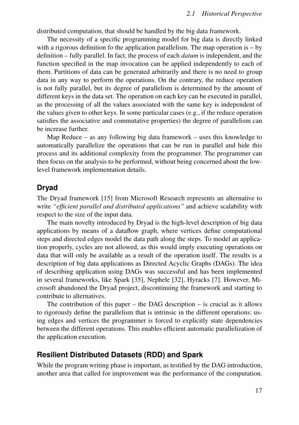
distributed computation, that should be handled by the big data framework.The necessity of a specific programming model for big data is directly linked
with a rigorous definition fo the application parallelism. The map operation is – bydefinition – fully parallel. In fact, the process of each datum is independent, and thefunction specified in the map invocation can be applied independently to each ofthem. Partitions of data can be generated arbitrarily and there is no need to groupdata in any way to perform the operations. On the contrary, the reduce operationis not fully parallel, but its degree of parallelism is determined by the amount ofdifferent keys in the data set. The operation on each key can be executed in parallel,as the processing of all the values associated with the same key is independent ofthe values given to other keys. In some particular cases (e.g., if the reduce operationsatisfies the associative and commutative properties) the degree of parallelism canbe increase further.
Map Reduce – as any following big data framework – uses this knowledge toautomatically parallelize the operations that can be run in parallel and hide thisprocess and its additional complexity from the programmer. The programmer canthen focus on the analysis to be performed, without being concerned about the low-level framework implementation details.
Dryad
The Dryad framework [15] from Microsoft Research represents an alternative towrite “efficient parallel and distributed applications” and achieve scalability withrespect to the size of the input data.
The main novelty introduced by Dryad is the high-level description of big dataapplications by means of a dataflow graph, where vertices define computationalsteps and directed edges model the data path along the steps. To model an applica-tion properly, cycles are not allowed, as this would imply executing operations ondata that will only be available as a result of the operation itself. The results is adescription of big data applications as Directed Acyclic Graphs (DAGs). The ideaof describing application using DAGs was successful and has been implementedin several frameworks, like Spark [35], Nephele [32], Hyracks [7]. However, Mi-crosoft abandoned the Dryad project, discontinuing the framework and starting tocontribute to alternatives.
The contribution of this paper – the DAG description – is crucial as it allowsto rigorously define the parallelism that is intrinsic in the different operations: us-ing edges and vertices the programmer is forced to explicitly state dependenciesbetween the different operations. This enables efficient automatic parallelization ofthe application execution.
Resilient Distributed Datasets (RDD) and Spark
While the program writing phase is important, as testified by the DAG introduction,another area that called for improvement was the performance of the computation.
17
Chapter 2. Historical Perspective on Big Data
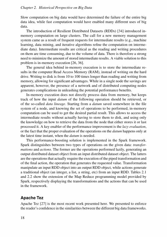
Slow computation on big data would have determined the failure of the entire bigdata idea, while fast computation would have enabled many different uses of bigdata.
The introduction of Resilient Distributed Datasets (RDDs) [34] introduced in-memory computation on large clusters. The call for a new memory managementsystem came as a result of frequent requests for intermediate results (e.g., machinelearning, data mining, and iterative algorithms refine the computation on interme-diate data). Intermediate results are critical as the reading and writing procedureson them are time consuming, due to the volume of data. There is therefore a strongneed to minimize the amount of stored intermediate results. A viable solution to thisproblem is in-memory execution [26, 36].
The general idea behind in-memory execution is to store the intermediate re-sults in the computer Read Access Memory (RAM), instead of writing on the harddrive. Writing to disk is from 10 to 100 times longer than reading and writing frommemory, allowing for significant advantages. While in a single node the savings areapparent, however, the presence of a network and of distributed computing nodesgenerates complications in unleashing the potential performance benefits.
In-memory execution does not directly process data from memory, but keepstrack of how the input datum of the following operation should be retrieved, orof the so-called data lineage. Starting from a datum saved somewhere in the filesystem of a node, and knowing the set of operations to be performed, in-memorycomputation can be used to get the desired partial result. This allows to access theintermediate results without actually having to store them to disk, and using onlythe knowledge on how to retrieve the data from the node that either stores it or lastprocessed it. A key enabler of the performance improvement is the lazy evaluation,or the fact that the proper evaluation of the operations on the datum happens only atthe latest time instant, when the datum is needed.
This performance-boosting solution is implemented in the Spark framework.Spark distinguishes between two types of operations on the given data: transfor-
mations and actions. The former are the operations performed lazily, generating anoutput distributed dataset object from an input distributed dataset object. The lattersare the operations that actually require the execution of the piped transformation andof the final action, the operation that generates the requested value. Transformationmanipulate an input RDD object into an output RDD object, while actions generatea traditional object (an integer, a list, a string, etc) from an input RDD. Tables 2.1and 2.2 show the extension of the Map Reduce programming model provided bySpark, respectively displaying the transformations and the actions that can be usedin the framework.
Apache Tez
Apache Tez [27] is the most recent work presented here. We presented to enforcethe reader’s confidence in the similarities between the different big data frameworks.
18
2.2 First-Principles of Big Data Processing
More precisely, Apache Tez helps us showing that all the big data frameworks arebuilt on the same concepts and components. Tez, in fact, is a “library to build data-
flow based engines” and can be used to produce code to be executed using differentframeworks: Map Reduce, Hive, Pig, Spark, Flik, Cascading, and Scalding. Tezconfirms the “intuition that most of the popular vertical engines can leverage a
core set of building blocks”.This idea is the basis of our systemic approach, and reinforces the importance
of looking for the common characteristics of all the frameworks, the first-principlesthat rule the processing of big data. Specifically, according to the creators of Tez,the common elements to the different frameworks are:
• A description of big data applications in the form of DAGs,
• The environment in which they run, Hadoop4 and the Hadoop File SystemHDFS 2.1, and a policy for resource allocation – in most cases ApacheYARN [29],
• Mechanisms for recovering from hardware failures,
• Mechanisms for publishing metrics and statistics.
We will not delve into further details of Apache Tez, but will limit our historicalperspective to highlighting the consciousness that different frameworks are basedon the same basic blocks. The following section is devoted to the clarification ofthese first principles.
2.2 First-Principles of Big Data Processing
The two most important breakthroughs in big data technologies so far have been:(1) the Map Reduce programming model, and (2) the DAG abstraction for programdescription. The validity of this statement is supported by the need to exploit par-allelism in big data applications. The two mentioned contributions are related toone of the forms of parallelism found in big data applications, that we defined insection 1.3. On one hand we have application-level parallelism, or parallelism thatarises from the possibility of executing multiple parts of the application in parallel(e.g., retrieving the marks given to students in two different exams and computingtheir averages can be done in parallel). On the other hand we have data-level paral-
lelism, or parallelism that is intrinsic in the operation that is being executed on thedata (e.g., adding one to every element of a vector can be done in parallel).
This section focuses on how to distribute the computation over the cluster andshould help us undestanding what are the first principles of processing big data.
4 http://hadoop.apache.org/
19

Chapter 2. Historical Perspective on Big Data
While capturing first-principle phenomena for a physical problem is easy andfirst-principle equations come directly from the law of physics, in computing prob-lems finding first-principle phenomena is a difficult task. It is of course always pos-sible to describe microscopic behavior, at the level of the transistors, and modelcomputation using the laws of electromagnetism. However, this results in unprece-dented complexity, and the given models are of little or no use to control the macro-scopic phenomena like data moving from one location to another, or resources beingallocated to a computational unit. These macroscopic laws, in computing systems,are themselves part of the design choices and should be therefore devised at thedesign level [3, 21].
In fact, first-principles laws are useful in computing systems too. There is a niceparallelism between physical problems and computing problems, in that these lawsdepend on the chosen level of abstraction, which can be chosen according to theaspects that need to be captured for the given problem solution. For instance, tomodel the behavior of a gas we could either decide to model the single moleculesdynamics or to use the ideal gas theory. In the same way in computing we can gofrom modeling the physics of transistors to modeling the values of the variablesduring the computation. Our choice should then depend on which aspects of theproblem are relevant for our study.
In big data applications, the relevant phenomena are related to (1) the processingof data, (2) data locality, and (3) the transmission of data through the network. Inthis section we will justify this statement starting from the design choices related tothe programming model and the DAG description that characterize most (if not all)of the big data frameworks.
Exploiting Parallelism
Big data applications run on clusters (networks of computing machines) and usuallydo not get exclusive access to the hardware resources, being these computational ornetworking resources. There are several managers that handle the requests for re-sources received from concurrently running applications. Google, for instance, usesBorg [30]; the Hadoop environment adopted YARN [29] or Mesos5. These man-agers or resource schedulers receive resource requests and allocate units of compu-tational resources in the cluster, e.g. <2GB RAM, 1 CPU>. The choice of the amountof resources to be allocated is almost invariantly formulated at the application leveland met whenever possible at the cluster level.
A big data application that runs on a cluster distributes the different computationsteps, i.e., different processing operations to be executed on the big data. Thesecomputation steps are defined as the couple metadata (defined in Section 2.1) andoperations. The computational units receive the information (the couple of metadataand operations) and perform the given operation on the data that is identified by themetadata. According to the properties defined in Chapter 1, operations and metadata
5 http://mesos.apache.org
20
2.2 First-Principles of Big Data Processing
are small with respect to the actual data. When the computation steps are sent acrossthe network their contribution to the network load is negligible with respect thecontribution of the transfer of the actual data.
A good distribution of the computational load will try to assign to a physicalnode (a computer) the processing of the data stored in the same physical node. Thisis based on the principle that moving the computation is cheaper than moving the
data (see the HDFS architecture guide6). This is one of the reasons why the DAG isa useful abstraction of the big data application, as it allows to clearly identify whichoperations have to be performed on which data.
The DAG abstraction describes the flow of data through the operations and tothe file system calls. The representation of big data applications in forms of DAGsat the present stage is not unique. Equivalent DAGs represent the same sequenceof computation step, the difference between them representing different executionchoices. Those choices are related to what the DAG describes of the given applica-tion. A natural consequence of this property is that the DAG can be manipulated toimprove the computational efficiency of the application through better parallelismexploitation. Section 3.1 gives a more accurate description of the DAG model.
We illustrate the above concept with an example. An application is composedof three different operations. The first is operated on an input set. The second andthird are independent operations that are to be executed on the data that is the resultof the first operation. The big data framework can then choose different executionalternatives.
As a first approach, the input is read and the first operation is performed inparallel on parts of the input by different computational units (that differ from themachines7). The output of this first step is written on the file system. As a followingstep, the computational units are divided in two groups and to each group is assignedone of the two following operations, that can be executed in parallel. Following thisapproach, the intermediate dataset is read twice by the machines of the differentgroups and processed in parallel. The two final results are separately written on thefile system.
As a second approach, the computational units can be immediately divided intwo groups. Each group reads the input set and perform sequentially the first (equalfor the two sets) operation and a second assigned operation among the two. Follow-ing this second approach, the first operation is performed twice on each datum, butthere is no writing of the intermediate result on the file system – a procedure that iscomputationally heavy and imposes a lot of additional overhead.
There are other different possibilities depending also on eventual mathematicalproperties of the given operations. Each of these possibilities results in a different
6 https://hadoop.apache.org/docs/r1.2.1/hdfs_design.html7 In the author’s opinion, it would be proper to define the computational units as the purely sequential
computing machines that constitute the cluster (i.e. the cores of the machines). In current big dataframeworks, these computational units are running processes and are implemented as java threadshence not univocally associated to a CPU. Chapter 5 contains a few remarks on the matter.
21
Chapter 2. Historical Perspective on Big Data
DAG. Deciding when a DAG is optimal given a specific infrastructure is a problemoutside the scope of this thesis. In here, we are concerned only with capturing allthe given possibilities, to ensure a complete description of the problem.
The example shows very well the difference between the two forms of paral-lelism. In the first approach “the first instruction is performed in parallel on parts ofthe input”. This is the operation-level or data-level parallelism described in Chap-ter 1, Section 1.3. For example, in the case of a map operation, the data can bepartitioned arbitrarily and execution of operations could happen in parallel. Thisis usually called multiple data, single operation parallelism. In the example, thesecond step, i.e., the two parallel operations, is an example of application-level par-allelism, also called single data, multiple operations parallelism. At this step of theexecution both the forms of parallelism are present and the framework must manageand exploit them at the same time. The computational units must be divided in twogroups and the complete input set must be divided among the elements of both thefirst and second group.
2.3 Spark Programming Model
Different programming models for big data ara available [38, 16], but at the presentstage, these programming models are all inspired by the Map Reduce paradigm,and define some extensions on top of it, sharing most of the functionalities. Forinstance, the frameworks based on SQL-like8 queries (like Hive and Pig) translatethose queries in a set of operations described by a DAG [38].
In our model validation experiments, we use Spark as a big data framework,due to its customization and extensibility. We here then report the set of operationsthat are available in the Spark framework. As reported in Section 2.1, the Sparkprogramming model is based on the RDD memory abstraction.
The main available operations are listed in tables 2.1 and 2.29. Operations aredivided between transormations and actions with the distinction reported in Sec-tion 2.1. From the computational point of view, the most relevant feature of eachoperation is its degree of parallelism. We are also interested in identifying the sit-uations that require to shuffle the data. The former is related to the possibility toparallelize the processing as an intrinsic property of each functionality (or to data-parallelism), the latter to the necessity of performing write and read operations forre-organizing the data in the cluster.
To exploit data-level parallelism, Spark partitions the input set of an operation(or a stage, as we will discuss next) and distribute the operation among the com-putational units – the so called tasks. A task consists in a set of data-chunks of theoriginal input and in the instructions to perform on them.
8 Structured Query Language (SQL) is the language used for interrogating traditional databases.9 http://spark.apache.org/docs/latest/rdd-programming-guide.html
22

2.3 Spark Programming Model
In Spark, the necessity of shuffling the data at a given point of the execution ofthe application is enforced if the next operation requires a different partition of thedataset (with respect to the one used for the pervious operation). In this case dataare centrally re-organized through serialization of the RDD in the file system, andsuccessive re-distribution of data chunks to the computational units. Spark evaluatesthis necessity of shuffle operations when building the application’s DAG. Considerfor instance the sequence of a map and a reduce operations: between the two ashuffle must be performed in order to aggregate the data with the same key. TheDAG must capture this aspect10. What requires a shuffle operation is that a differentpartition of the dataset is required.
For our purposes, we are interested in how each operation is characterized interms of level of parallelism that allows to framework to execute it separately in thedifferent chunks of input data. We are also interested in knowing which operationsrequire input from the file system or write their output on the file system.
Spark’s application DAG
As written in Section 2.1, the use of dataflow diagrams in big data applicationswas introduced in the Dryad framework. Dryad enforced a dataflow programmingmodel, creating a one-to-one mapping between the application and its DAG. Theprogrammer is supposed to use a precise programming syntax to build the DAG –and the application itself. Each vertices defines a set of sequential operations to beperformed on data (which are encoded as the edges entering vertices). The edgesexiting from nodes point to the nodes that use the output of the given node as input.In Dryad, the DAG is only a model of the program, and does not represent anythingabout its execution. In successive frameworks, the DAG was automatically extractedand built by the big data framework based on the application code.
Since in our experiments we use Spark, this section explains how the DAG isgenerated from the application code in the Spark framework.
The DAG is used to represent the parallelism that characterizes the applicationwe are considering and the read and write operations. Spark uses the actions topartition the application in jobs: this means that each job, given the definition oftransformations and actions, starts from one or more RDD (a big data object), andperforms different transformations on them, concluding with the action that gener-ates a value.
The sequence of transformations in each job is described by a DAG. A transfor-mation is applied on the input RDD – separately on its subsets (the performing ofeach of those is what we named in section 2.1 as task). If multiple operations can besequentially performed on the same subset of data, they are grouped and performed
10 A particular case is the one when the reduce operation satisfies the associativity property: nodes couldstart performing the reduce operation of the data stored in themselves and only after this perform theshuffle, possibly strongly reducing the volume of data to redistribute through the network.
23

Chapter 2. Historical Perspective on Big Data
Table 2.1 Spark: list of transformations.
Transformation Meaningmap(func) Return a new distributed dataset formed by passing each element of the
source through a function func.filter(func) Return a new dataset formed by selecting those elements of the source
on which func returns true.flatMap(func) Similar to map, but each input item can be mapped to 0 or more output
items (so func should return a Seq rather than a single item).mapPartitions(func) Similar to map, but runs separately on each partition (block) of the
RDD, so func must be of type Iterator<T> => Iterator<U> when run-ning on an RDD of type T.
mapPartitionsWithIndex(func)
Similar to mapPartitions, but also provides func with an integer valuerepresenting the index of the partition, so func must be of type (Int,Iterator<T>) => Iterator<U> when running on an RDD of type T.
sample(withReplacement,fraction, seed)
Sample a fraction fraction of the data, with or without replacement, us-ing a given random number generator seed.
union(otherDataset) Return a new dataset that contains the union of the elements in thesource dataset and the argument.
intersection(otherDataset) Return a new RDD that contains the intersection of elements in thesource dataset and the argument.
distinct([numTasks]) Return a new dataset that contains the distinct elements of the sourcedataset.
groupByKey([numTasks]) When called on a dataset of (K, V) pairs, returns a dataset of (K, Iter-able<V>) pairs.
reduceByKey(func, [num-Tasks])
When called on a dataset of (K, V) pairs, returns a dataset of (K, V) pairswhere the values for each key are aggregated using the given reducefunction func, which must be of type (V,V) => V. Like in groupByKey,the number of reduce tasks is configurable through an optional secondargument.
aggregateByKey(zeroValue)(seqOp, combOp, [num-Tasks])
When called on a dataset of (K, V) pairs, returns a dataset of (K, U)pairs where the values for each key are aggregated using the given com-bine functions and a neutral "zero" value. Allows an aggregated valuetype that is different than the input value type, while avoiding unnec-essary allocations. Like in groupByKey, the number of reduce tasks isconfigurable through an optional second argument.
sortByKey([ascending],[numTasks])
When called on a dataset of (K, V) pairs where K implements Ordered,returns a dataset of (K, V) pairs sorted by keys in ascending or descend-ing order, as specified in the boolean ascending argument.
join(otherDataset, [num-Tasks])
When called on datasets of type (K, V) and (K, W), returns a dataset of(K, (V, W)) pairs with all pairs of elements for each key. Outer joins aresupported through leftOuterJoin, rightOuterJoin, and fullOuterJoin.
cogroup(otherDataset,[numTasks])
When called on datasets of type (K, V) and (K, W), returns a datasetof (K, (Iterable<V>, Iterable<W>)) tuples. This operation is also calledgroupWith.
cartesian(otherDataset) When called on datasets of types T and U, returns a dataset of (T, U)pairs (all pairs of elements).
pipe(command, [envVars]) Pipe each partition of the RDD through a shell command, e.g. a Perl orbash script. RDD elements are written to the process’s stdin and linesoutput to its stdout are returned as an RDD of strings.
coalesce(numPartitions) Decrease the number of partitions in the RDD to numPartitions. Use-ful for running operations more efficiently after filtering down a largedataset.
24

2.3 Spark Programming Model
Action Meaningrepartition(numPartitions) Reshuffle the data in the RDD randomly to create either more or fewer
partitions and balance it across them. This always shuffles all data overthe network.
repartitionAndSortWithinPartitions(partitioner)
Repartition the RDD according to the given partitioner and, within eachresulting partition, sort records by their keys. This is more efficient thancalling repartition and then sorting within each partition because it canpush the sorting down into the shuffle machinery.
Table 2.2 Spark: list of actions.
Action Meaningreduce(func) Aggregate the elements of the dataset using a function func (which takes
two arguments and returns one). The function should be commutativeand associative so that it can be computed correctly in parallel.
collect() Return all the elements of the dataset as an array at the driver program.This is usually useful after a filter or other operation that returns a suf-ficiently small subset of the data.
count() Return the number of elements in the dataset.first() Return the first element of the dataset (similar to take(1)).take(n) Return an array with the first n elements of the dataset.takeSample(withReplace,num, [seed])
Return an array with a random sample of num elements of the dataset,with or without replacement, optionally pre-specifying a random num-ber generator seed.
takeOrdered(n, [ordering]) Return the first n elements of the RDD using either their natural orderor a custom comparator.
saveAsTextFile(path) Write the elements of the dataset as a text file (or set of text files) ina given directory in the local filesystem, HDFS or any other Hadoop-supported file system. Spark will call toString on each element to con-vert it to a line of text in the file.
saveAsSequenceFile(path)(Java and Scala)
Write the elements of the dataset as a Hadoop SequenceFile in a givenpath in the local filesystem, HDFS or any other Hadoop-supported filesystem. This is available on RDDs of key-value pairs that implementHadoop’s Writable interface. In Scala, it is also available on types thatare implicitly convertible to Writable (Spark includes conversions forbasic types like Int, Double, String, etc).
saveAsObjectFile(path)(Java and Scala)
Write the elements of the dataset in a simple format using Java serial-ization, which can then be loaded using SparkContext.objectFile().
countByKey() Only available on RDDs of type (K, V). Returns a hashmap of (K, Int)pairs with the count of each key.
foreach(func) Run a function func on each element of the dataset. This is usually donefor side effects such as updating an Accumulator or interacting withexternal storage systems.
25
Chapter 2. Historical Perspective on Big Data
together in a single task. When a transformation requires input from multiple parti-tions, data must be re-organized, i.e. stored and re-partitioned, via a shuffle.
Shuffles delimit what in the Spark framework is called a stage. Each stage cor-responds to a node in the DAG. More formally, a stage is a sequence of transforma-tions at the end of which a shuffle (or an action in the case of the final stage of thejob) must be performed. The flow of data into the stages is described by the directededges: an edge from stage 1 to stage 2 defines that the output of stage 1 is the inputof stage 2.
As frequently happens in interactive algorithms and machine learning appli-cations different jobs may require the same operations on the same data (henceproducing the same intermediate result). Spark avoids performing twice these oper-ations, re-using the already produced RDD — the key concept of in memory exe-cution of Spark defined in section 2.1. This means that the DAGs of different jobscan be connected11.
The framework can then operate manipulations on the DAG to optimize its exe-cution, but we will not delve in further detail as it is not strictly related to our work.The key points in Spark are the automatical retrieval of the DAG from the applica-tion code and the fact that this description is not unique. Optimizations performedon the DAG are usually aimed at minimizing read and write operations. Also, theydo not strictly depend on the cluster and on the available resources, but rather onthe data and the sequence of operations.
2.4 Performance and Simulation of Big Data Frameworks
The previous sections have provided an overview of how a big data frameworkworks. It is a complex, distributed system that runs in a complex environment, acluster of ten, hundred of even thousands of machines. Predicting the behavior ofboth the software and the hardware is a non-trivial task. However, as we stated inChapter 1, Section 1.5, the ability to predict and even control the execution of anapplication would give us a clear advantage. This need is further witnessed by theexistence of several works, related to either performance modeling or simulationof big data frameworks. Here we report just a small part of them in chronologicalorder.
• Mumak (2009)12: is the Apache open source simulator for Hadoop.
• MRperf (2009)13: is a Map Reduce simulator by Virginia Tech researchers,
11 Spark does not actually connect the DAG of different jobs: in case the described scenario happens itintroduces the stages twice, but executes them only once re-using the available data. This is equivalentto connecting the DAGs.
12 https://issues.apache.org/jira/browse/MAPREDUCE-72813 http://research.cs.vt.edu/dssl/mrperf/
26
2.4 Performance and Simulation of Big Data Frameworks
the purpose of this simulator is to help programmers evaluating different set-up choices on the Hadoop cluster.
• SimMR (2011) [31]: another Map Reduce simulator oriented at allowing theanalysis of different schedulers.
• YARNsim (2015) [22]: a simulator oriented at emulating the behavior ofMapReduce in the YARN environment introduced in 2013.
• I/O modeling for big data applications over cloud infrastructures (2015) [25]:This works discusses a performance analysis and points out the difficulties incapturing the implementation intricacies of big data applications, proposinga purely input output approach for performance modeling.
• Analysis, Modeling, and Simulation of Hadoop YARN Map Reduce(2016) [8]: a statistical modeling of Map Reduce in the YARN Hadoopenvironment.
• Stage Aware Performance Modeling of DAG Based in Memory Analytic Plat-forms (2016) [14]: a gray-box approach for analyzing the performance ofSpark applications based on the DAGs produced by the framework. The ex-ecution time of each stage of the DAG is statistically modeled running theoperations on subsets of the input.
These are only a few works that demonstrate the importance of the topic. Whatis crucial is that none of these approaches exhibits an explicit system-theoreticalapproach, resulting in the fact that none of the presented models is dynamical.The proposals are purely statistical approaches or simulation-based analysis tools.They do not investigate abstractions or first-principle relations between the involvedquantities. Despite that, similar considerations (e.g., the relevance of the degree ofconcurrency or of the data locality) are recurrent in the different studies. Modelsof phenomena are often derived from data observations, not from a systemic anal-ysis of the involved quantities. For instance YARNsim [22] evidences a lognormaldistribution of the execution time for map tasks with the average value linearly re-lated to: (1) blocksize of input chunks, (2) size of intermediate data and (3) levelof concurrency. In our opinion these work lack investigation on why these relationsemerge, probabilistic distributions of certain quantities, and system dynamics.
27

3
Modelling Big Data
Frameworks
To process the large amount of data typically involved in big data computations, datastorage needs to be distributed onto different physical nodes in a cluster and dupli-cated for fault tolerance. At the same time, to obtain competitive performance, dataprocessing must exploit parallelism. The combination of these two factors supportsthe use of a distributed software architecture with multiple storage and computationnodes.
These nodes concurrently contribute to the processing of the data. With the termdata processing we indicate the execution of an application that contains one ormore calls that operate on the large data set, typically executing instructions thatread, write, or modify the data.
We will use first-principle models, describing only the core physics of the bigdata framework – which does not depend on the specific implementation frame-work. Traditionally first-principle models are defined as the models based on bal-ance equations. In our model this kind of equation are in fact present in three ways:when modeling (1) the progression of the computation, (2) data transmission amongthe different computational steps and (3) resource allocation.
In this Chapter, we derive a generic abstract model for the execution of an appli-cation in a big data framework, and we propose some specialization of the abstractmodel to describe specific framework implementations, like Apache Spark. We willuse a toy example to describe the main steps for retrieving the model from the codeof a big data application.
3.1 Big Data Application
The source code of a big data application contains multiple calls to functions thatmanipulate the data, like map, filter, reduce, and their derivatives. These callsare resolved in the scope of the framework, that has access to the code that it should
28

3.1 Big Data Application
1 text = read_input(in1_location) // Call #1
2 counts = text.flatmap(fun line -> line.split(" ")) // Call #2a
3 .map(fun word -> (word, 1)) // Call #2b
4 .reducebykey(fun a, b: a+b) // Call #2c
5 counts.write_output(out1_location) // Call #3
6 articles = {a, an, the}
7 no_articles =
8 text.flatmap(fun line -> line.split(" ")) // Call #4a
9 .filter(fun word not in articles) // Call #4b
10 no_articles.write_output(out2_location) // Call #5
Listing 3.1 Pseudo-code for a big data application example.
(potentially optimize and) execute. Sequences of instructions containing frameworkcalls are interleaved with other operations that the application should execute.
For example, the code for the application shown in Listing 3.1 contains fivesequences of big data framework calls. The first one reads an input text from agiven location (Call #1). The second one splits each line of the text into wordswith a flatmap (Call #2a), transforms each word into a tuple with the word asa key and a number 1 as a value with a map operation (Call #2b) and counts thenumber of occurrencies of each word with a reducebykey call (Call #2c). Thethird call writes the the counts to an output location (Call #3). The fourth callparses the text dividing it into words with the flatmap function (Call #4a) andthen removes the articles using a filter function (Call #4b). Finally, the last callsaves the text without articles to a given location (Call #5).
Looking at the specific calls, it is possible to identify the input and the outputdata of each operation. These create a logic link between the different calls, thatdepend upon each other for execution. We can represent each of the frameworkcalls as the node of a graph, and the dependencies as directed edges between nodes.
Arrows represent dependancies related to big data sets. Those data sets are gen-erally transmitted through the different functions being written on the distributedfile system, hence a write and a read operations are required. If the intermediate da-
tum is small enough that it doesn’t require distributed storage the it doesn’t requireto be written on the file system and can instead be stored locally1. For this reasonin such cases no arrow connection between the nodes related to the function callsis required. Under the light of this statement the DAG becomes a representation ofboth the program and its execution.
DAG Definition
The result of the analysis in the previous paragraph is a Directed Acyclic Graph,which both represents the order of execution of the function calls in the framework
1 In general further processing of those data wont even require more calls of the framework functions.
29

Chapter 3. Modelling Big Data Frameworks
#1
#2a #2b #2c #3
#4a #4b #5
text
counts
text
no_articles
Figure 3.1 A Directed Acyclic Graph models the framework calls of the applica-tion shown in Listing 3.1.
and the read write operations to the file system. This abstraction is more general thanthe one presented in Chapter 2 for frameworks like Apache Spark, Apache Tez, andDryad as it is generated from the generic code and not defined by the framework.For this reason it can theoretically be applied also to the execution of application inframeworks that do not explicitly implement the DAG.
Nodes of the DAG represent calls that should be executed, while arrows repre-sent synchronization points between the function calls executions, that model theneed for input data that should be written on the file system by the execution ofprevious function calls. Figure 3.1 represent the DAG of the code block in List-ing 3.1. Dashed arrows and gray marks are added only for convenience to representthe entry and exit point of the code block execution and to highlight that this isonly a code block in a possibly larger application. On top of the directed edges, wehave identified the name of the variables associated with the data exchanged by theframework function calls. Assuming we know the control flow of the big data ap-plication, we can model the big data framework calls that are going to be executedby any application using a DAG2.
Formally, se use the following notation.
• Definition (Directed Graph): A Directed Graph is a tuple < V,E > whereV = {v1,v2, . . .vn} is a set of n vertices or nodes, and E is a set of directededges, each of which can be written as vx → vy, indicating a connection be-tween the nodes vx and vy both in V , where vx is the start point and vy is theend point of the edge.
• Definition (Path): A path in a directed graph is a sequence of vertices thatare connected with directed edges. For example, if V = {v1,v2,v3} and E ={v1 → v3,v2 → v3,v3 → v1}, a possible path is the sequence [v2,v3,v1,v3].
2 Our aim is to verify properties related to the execution time of the big data application. The assump-tion of knowing the control flow is therefore not a limiting one, as we can run the verification processfor all the possible control flows of the application and observe the worst-case scenario. We still needit to know previous the the application execution which framework calls will be executed.
30
3.1 Big Data Application
• Definition (Cycle): A cycle is a path that starts and ends with the same node.
• Definition (Directed Acyclic Graph): A Directed Graph that has no cyclesis also referred to as a Directed Acyclic Graph (DAG).
• Definition (Input Edges of a Node): For each node vx we denote with E (vx)the set of directed edges that have the node as the end point. I (vx) = {vi →v j ∈ E | v j = vx}.
• Definition (Output Edges of a Node): For each node vx we denote withO(vx) the set of directed edges that have the node as the start point. O(vx) ={vi → v j ∈ E | vi = vx}.
• Definition (Node Predecessors): A node vx is said to belong to the set ofpredecessors of a node vy – denoted with P(vy) – when the arc vx → vy isincluded in the set of arcs of the DAG, i.e., if vx → vy ∈ E . In other terms,P(vy) = {vx | vx → vy ∈ I (vx)}.
• Definition (Node Successors): A node vx is said to belong to the set of suc-
cessors of a node vy – denoted with S (vy) – when the arc vy → vx is in-cluded in the set of arcs of the DAG, i.e., if vy → vx ∈ E . In other terms,S (vy) = {vx | vx → vy ∈ O(vx)}.
• Definition (Initial Nodes): The set of initial nodes I is defined as theset of nodes whose predecessors sets are empty. Formally, a node vx ∈I iff P(vx) =∅.
• Definition (Final Nodes): The set of final nodes F is defined as the set ofnodes whose successors sets are empty. Formally, a node vx ∈F iff S (vx) =∅.
We refer to the application DAG as defined above (that is with a one-to-one cor-respondence between nodes and function calls) using the term “fine-grained DAG”.Irregardless of the execution framework, for every block of code, we can alwaysdetermine the fine-grained DAG of the application. In some frameworks, the (fine-grained) DAG is manipulated (either at compile or run time) to enable further op-timizations, with the aim of reducing computation time, and increasing efficiency.This improvement is possible as the DAG is not only a model of the program butcaptures also the input output operations on the file system.
The information included in the DAG for each node is (1) the function call thatthe nodes represent, (2) its input edges, and (3) output edges. The function callrepresents the operation that the big data framework is applying to the data and canbe selected among the ones available for the specific big data framework. The inputand output edges – I (vx) and O(vx) – model the data needed for the computationand produced by the computation.
31

Chapter 3. Modelling Big Data Frameworks
DAG Manipulations
If we let a single node represent a sequence of function calls instead of a single one,we can define optimizations on the DAG. In this case, we interpret the edges as thedefinition of the input ad output sets of the given sets of operations and we can defineall the possible mutations that are applicable to a given graph. The transition from asingle function calls to a set of calls models the execution of multiple operations onthe same partition of the data without the need for intermediate operations involvingwriting results. This enables optimizations like recomputing a set of data instead oftransferring the data over the network. We now investigate the possible maniplationsof the DAG.
• Join of two nodes: a node can be joined with its successor if the set of suc-cessors contains only that specific node and the node is the only predeces-sor of its successor. In place of the two nodes, one single node remains inthe DAG, representing the sequence of operations of the two joint nodes.The predecessors of this joint node are the predecessors of the first nodeand the successors of the joint node are the successors of the original suc-cessor node. The new DAG describes exactly the same sequence of opera-tions but hides the intermediate result that would be generated between thetwo operations, avoiding the read and write operations of it. For this rea-son the join two nodes manipulation is applicable only if the one to onerelation is satisfied. The necessity but not sufficiency is related to the pos-sibility that two successive operations might require read and write opera-tions in between for data shuffling. Formally, given a DAG D =<V,E > andtwo nodes vx,vy ∈ V such that S (vx) = {vy} and P(vy) = {vx} we can de-fine a new DAG D′ =< V ′,E ′ > with V ′ = V
⋃
vz \ {vx,vy} and E ′ such thatP(vz) = P(vx) and S (vz) = S (vy)
3.
• Duplicate a node with respect to the input: every node with strictly morethan one successor can be split in two nodes characterized by the same opera-tions and same predecessors. The sets of the successors of the new nodes mustbe a partition of the successors set of the single node. The two resulting nodesare associated with the same operation that defined the starting one. This ma-nipulation models the simple choice of executing twice the same operationson the same dataset (possibly in parallel on different computation units). Forthis reason it can always be applied. Formally, given a DAG D =< V,E >and a node vx ∈ V with S (vx) = {vy,i|i = 1,s} we can define a new DAGD′ =< V ′,E ′ > where V ′ = V
⋃{vx.i|i = 1, . . . ,s} \ vx and E ′ is such thatP(vx) = P(vx,1) = . . .= P(vx,s)
4 and S (vx,i) = {vy,i} , i = 1, . . . ,s.
3 P(vx) and S (vy) are defined in D while P(vz) and S (vz) are defined in D′4 P(vx) is defined in D while P(vx,i) are defined in D′
32

3.1 Big Data Application
• Duplicate a node with respect to the output: this manipulation is the dualof the former. It is operated on a node with strictly more than one predecessorand consist in applying the operation separately to the different outputs of thepredecessors. The successors set of each of the new nodes must coincide withthe one of the single node. The two resulting nodes are associated with thesame operation of the starting one. Differently from the previous manipula-tions, this one cannot always be applied depending on the nature of the func-tion calls that are associated to the node to be duplicated5. Formally, given aDAG D =< V,E > and a node vy ∈ V with P(vy) = {vx,i|i = 1, p} we dandefine a new DAG D′ =<V ′,E ′ > where V ′ =V
⋃{vy.i|i = 1, . . . , p}\ vy andE ′ is such that S (vy) = S (vy,1) = . . . = S (vx,p) and
⋃
i=1,...,p{P(vy,i)} ={vx,i|i = 1, . . . , p}.
• Switch two nodes: a node can be switched with its successor if this is the onlysuccessor of the considered node and the node is the only predecessor of itssuccessor. Moreover, it is required that the two operations satisfy the commu-tativity property. Formally, given a DAG D =<V,E > and two nodes vx,vy ∈V such that S (vx) = {vy}, P(vy) = {vx}, P(vx) = {vpr,i|i = 1, . . . , p} andS (vy) = {vsc,i|i = 1, . . . , p} we can define a new DAG D′ =<V,E ′ > whereE ′ is such that S (vy) = {vx}, P(vx) = {vy}, P(vy) = {vpr,i|i = 1, . . . , p}and S (vx) = {vsc,i|i = 1, . . . , p}
The described manipulations are strictly related to how the graph models theapplication in terms of the sequence of operations that are given a specific set ofinput and output data. Using these manipulations, we are able to describe all (butnot only) the possible graphs that are related to the given code. The fundamentalproperty that must be guaranteed while manipulating the DAG is that the resultingprograms always provide the same result. This concept is used to define the equiv-
alence between two DAGs.
• Definition: Equivalent DAGs Two DAGs are said to be equivalent when thesequences of operations they define applied to the any input produces thesame output6.
By means of those manipulations we can model how the sequences of frame-work calls discussed can be grouped into different “blocks of calls”, depending onthe big data framework compiler logic and on memory access.
In the example of Figure 3.1 we can apply the join two nodes manipulation toboth the branches of the DAG: three times to the upper branch grouping operations
5 The operation must allow independent processing of each of the resulting subsets of the input set,that is the degree of parallelism must allow it.
6 Note that equivalence is related to what the DAG describes of the definition of the program, not ofits execution.
33
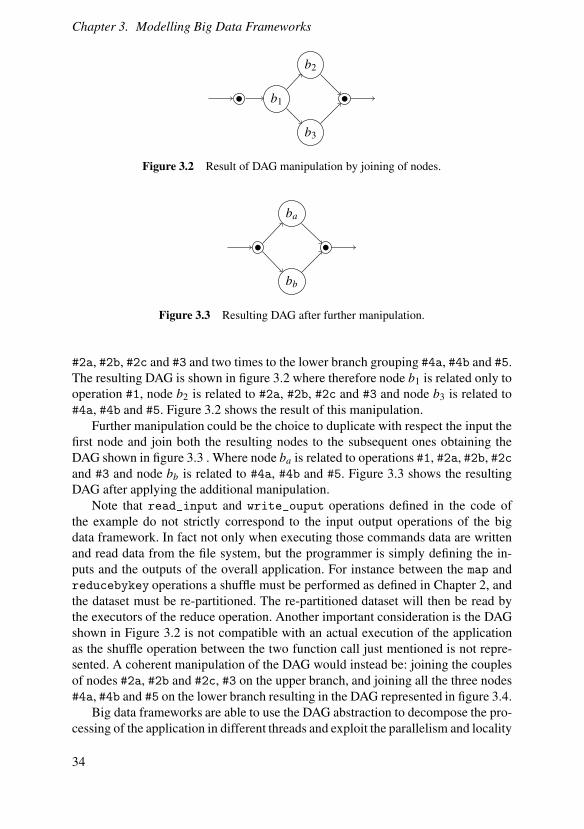
Chapter 3. Modelling Big Data Frameworks
b1
b2
b3
Figure 3.2 Result of DAG manipulation by joining of nodes.
ba
bb
Figure 3.3 Resulting DAG after further manipulation.
#2a, #2b, #2c and #3 and two times to the lower branch grouping #4a, #4b and #5.The resulting DAG is shown in figure 3.2 where therefore node b1 is related only tooperation #1, node b2 is related to #2a, #2b, #2c and #3 and node b3 is related to#4a, #4b and #5. Figure 3.2 shows the result of this manipulation.
Further manipulation could be the choice to duplicate with respect the input thefirst node and join both the resulting nodes to the subsequent ones obtaining theDAG shown in figure 3.3 . Where node ba is related to operations #1, #2a, #2b, #2cand #3 and node bb is related to #4a, #4b and #5. Figure 3.3 shows the resultingDAG after applying the additional manipulation.
Note that read_input and write_ouput operations defined in the code ofthe example do not strictly correspond to the input output operations of the bigdata framework. In fact not only when executing those commands data are writtenand read data from the file system, but the programmer is simply defining the in-puts and the outputs of the overall application. For instance between the map andreducebykey operations a shuffle must be performed as defined in Chapter 2, andthe dataset must be re-partitioned. The re-partitioned dataset will then be read bythe executors of the reduce operation. Another important consideration is the DAGshown in Figure 3.2 is not compatible with an actual execution of the applicationas the shuffle operation between the two function call just mentioned is not repre-sented. A coherent manipulation of the DAG would instead be: joining the couplesof nodes #2a, #2b and #2c, #3 on the upper branch, and joining all the three nodes#4a, #4b and #5 on the lower branch resulting in the DAG represented in figure 3.4.
Big data frameworks are able to use the DAG abstraction to decompose the pro-cessing of the application in different threads and exploit the parallelism and locality
34

3.2 Model of the Computational Step
c0
c1 c2
c3
Figure 3.4 DAG manipulated taking into account the shuffle.
of data to improve computing performances. The application is first decomposed inthe different computational steps7 corresponding to the nodes of the DAG. Each ofthe computational steps is decomposed in different parallel processes8. This is howthe DAG abstraction allows the big data framework to exploit the two forms of par-allelism. In the next section we will propose a dynamical model for the distributedprocessing of each of the computational steps.
3.2 Model of the Computational Step
The DAG abstraction allows us to model the application as a set of computing steps(the nodes) that synchronize and exchange information (the edges). The processingof each of those steps is distributed according to the degree of parallelism allowedby the operations that define it. This means that there are different executors for thesame computational step and that each of them performs the given operations on asubset of the input of the overall node9.
The allocation and synchronization of these executors is the level at which wewish to exploit data locality, i.e., a good big data framework will try to allocate theexecutors in the cluster close to where the data they are supposed to process arelocated. On the one side, data locality has a strong impact on the execution of theapplication. On the other side, it strongly depends on the specific execution instanceand on the cluster on which the application is run. For those reasons we chose forour model a higher level of abstraction that is oblivious to this phenomenon10.
We generically define the given resources as a single variable and relate theprogress of data processing to this single variable, being it executors, cores, CPUtime and so forth. The resources are then assigned to the overall computational step(or stage in Spark jargon). If we want to regulate the amount of resources with a
7 In Spark, computational steps are called stages.8 In Spark, parallel processes are called tasks.9 The union of the subsets must be the original input set.
10 The retrieved model can be extended and overcome this limitation, as explained in Chapter 5.
35
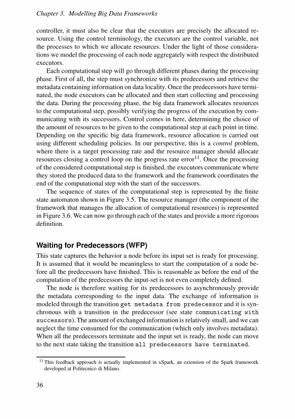
Chapter 3. Modelling Big Data Frameworks
controller, it must also be clear that the executors are precisely the allocated re-source. Using the control terminology, the executors are the control variable, notthe processes to which we allocate resources. Under the light of those considera-tions we model the processing of each node aggregately with respect the distributedexecutors.
Each computational step will go through different phases during the processingphase. First of all, the step must synchronize with its predecessors and retrieve themetadata containing information on data locality. Once the predecessors have termi-nated, the node executors can be allocated and then start collecting and processingthe data. During the processing phase, the big data framework allocates resourcesto the computational step, possibly verifying the progress of the execution by com-municating with its successors. Control comes in here, determining the choice ofthe amount of resources to be given to the computational step at each point in time.Depending on the specific big data framework, resource allocation is carried outusing different scheduling policies. In our perspective, this is a control problem,where there is a target processing rate and the resource manager should allocateresources closing a control loop on the progress rate error11. Once the processingof the considered computational step is finished, the executors communicate wherethey stored the produced data to the framework and the framework coordinates theend of the computational step with the start of the successors.
The sequence of states of the computational step is represented by the finitestate automaton shown in Figure 3.5. The resource manager (the component of theframework that manages the allocation of computational resources) is representedin Figure 3.6. We can now go through each of the states and provide a more rigorousdefinition.
Waiting for Predecessors (WFP)
This state captures the behavior a node before its input set is ready for processing.It is assumed that it would be meaningless to start the computation of a node be-fore all the predecessors have finished. This is reasonable as before the end of thecomputation of the predecessors the input-set is not even completely defined.
The node is therefore waiting for its predecessors to asynchronously providethe metadata corresponding to the input data. The exchange of information ismodeled through the transition get metadata from predecessor and it is syn-chronous with a transition in the predecessor (see state communicating with
successors). The amount of exchanged information is relatively small, and we canneglect the time consumed for the communication (which only involves metadata).When all the predecessors terminate and the input set is ready, the node can moveto the next state taking the transition all predecessors have terminated.
11 This feedback approach is actually implemented in xSpark, an extension of the Spark frameworkdeveloped at Politecnico di Milano.
36

3.2 Model of the Computational Step
WFP
PD
CWS
E
all predecessors have terminated
get metadata from predecessor
finished processing
all successors have been informed
inform successor (send metadata)
Figure 3.5 State machine representing the states of the single computational step.
RA de-allocate resources to step-iallocate resources to step-i
Figure 3.6 State machine of resource allocator.
Processing Data (PD)
In this state we capture the processing of the data. The processing speed depends onthe allocated resources. Resources u(t) – like CPU time and cores – are assigned toexecutors, that process the data. We model the progress rate as an integrator wherethe integration rate is a generic function of the allocated resources g(·).
An example ise(t) = g(e(t),u(t),d(t),θ ) , (3.1)
where e(t) represents the state variable (the computation progress), u(t) are the allo-cated resources, d(t) is a positive quantity that represents a time varying efficiencyof the computation and θ is a vector of parameter describing the cluster.
37

Chapter 3. Modelling Big Data Frameworks
The time varying efficiency is a disturbance on the system representing all thepossible external inputs affecting the computation progress, from the varying dataload to the external disturbances acting on the cluster’s machines. The function g()must be non negative12 and saturated with respect to the input resources accordingto the maximum available computational parallelism in the overall cluster — i.e. thenumber of available sequential computational units, the cores — and the maximumparallelism allowed by the operations represented by the node.
The procedure of writing data on the file system is considered to happen imme-diately after the data are generated. It therefore overlaps with the processing timeand does not require specific modeling13. This holds under the assumptions that (1)the writing action doesn’t affect the processing rate, and (2) that the writing rate ishigher than the processing rate – i.e. the bottleneck is the processing.
When the variable e(t) reaches the threshold representing the volume of inputdata the node can take the transition finished processing and move to the nextstate.
Communicating with Successors (CWS)
This state is the dual of the Waiting for predecessors one, and models howthe node synchronizes with successors. The node takes the transition inform
successor once for each of the successors synchronizing with them and sharingthe metadata of its output-set. In the real case the metadata should describe datalocality and volume, to our level of abstraction is sufficient the latter. The volume ofgenerated data is defined by the fraction factor (a parameter of the node – and of theset of operations) multiplied by the volume of the input-set. Once all successors areinformed the node moves to the final state End (E) where it is eventually availablein case backup information are needed.
Resources and Resource Allocation Modeling
The model of the overall application is constituted by a set of parallel switchingsystems, equal to the one just presented. The DAG describes the required synchro-nization among these different switching systems, determining the successor andpredecessor relationships. Each of the switching systems models independently thecomputation of a single step. The different switching systems share the resources tothe same cluster, hence the sum of the allocated resources u(t) to each step must besaturated according to the cluster dimensions.
The Resource Manager can allocate resources with different policies, usually theprogrammer has several choices for each framework. The resource allocation policydetermines both when the the transitions allocate resources and de-allocate
12 A negative value of g() implies the loss of processed data during the application execution. Weassume this cannot happen, as the File System takes care of replicating data and guarantees faulttolerance.
13 This is even more valid when the computational unit is on a machine that works also as storage node.
38

3.3 Frameworks: the Resource Allocation
resources are taken and how much resources to which stage are allocated. In ourcontrol-theoretical perspective this is the control law.
A final note about the modeling of resources is that, as we stated in Chapter 1Section 2.2, those applications are not the only running on the cluster. We can easilyrepresent this making the saturation level of total resources vary in time.
3.3 Frameworks: the Resource Allocation
In this section we investigate how to apply the model just defined to the executionof applications defined in different frameworks. The basic ingredients for definingthe model are (1) the DAG definition and (2) the behavior of the Resource Manager.
For defining the resource manager behavior, we need to analyse the schedulerof the cluster environment in which applications run. All of the framework that wewill model run in an Hadoop environment in which the programmer is allowed toplug different scheduling policies. The standard policy is the FIFO scheduler thatdoes not use any feedback signal and simply allocates resources to all the tasks it re-ceives in the arrival order. This can be implemented in our model activating the tran-sition allocate resources, as long as the processing is not terminated and thereis resource available. Alternatives to this behavior are the “Fair scheduler”, devel-oped by Facebook, and the “Capacity scheduler”, developed by Yahoo!. These canbe modeled as an arbitrary activation of allocate resources (or de-allocateresources), providing the amount of resources to allocate at each activation.
We also model the allocation policy implemented in xSpark [4]. xSparx imple-ments a feedback-based resource allocator, described in the following.
xSpark Resource Allocator
The xSpark resource allocator implements a cascade control loop. The first loop isat the level of the overall application and acts on the deadline of the single sages– adjusting the deadlines for proper allocation. The second loop is local to eachcomputational step and allocates the resources.
Application Level Control Loop The deadline control loop generates the dead-line for each computational step (stage) using a heuristic approach, based on thedeadline of the overall application DA , supplied by the user. Denoting with T j thetime elapsed from the beginning of the processing at the beginning of stage j, thedeadline D j for the stage j is generated as show in Equation 3.2.
D j =α ·DA −T j
w j
(3.2)
Here, α is a constant parameter between 0 and 1, used to implement a givenmargin with respect of the overall deadline, and w j is a weight associated witheach stage, determined according to Equation 3.4. Denoting with R j the number of
39

Chapter 3. Modelling Big Data Frameworks
0, elaboration status
t
Prescribed completion %100
γ ·D j
D j, required completion time for j
Figure 3.7 Processing progress reference for stage j.
remaining stages to complete at the moment of the start of the execution of stagej, with r j the ratio between the expected duration of the stages that still need tobe executed and the duration of stage j’s computation, and with d j the expectedduration of stage j, the ratio is determined as
r j =1
d j
·n
∑i= j
di, (3.3)
and the stage weight is then defined as
w j = β ·R j +(1−β ) · r j. (3.4)
In Equation (3.4), β is a constant determined conducting a sensitivity analysis, inxSpark its value is set to 1
3 .
Stage Level Control Loop The inner control loop uses the deadline generated bythe external control loop to compute the reference of processing progress, with somesafety margin defined by the user like the one plotted in Figure 3.7. The margin isimplemented forcing the processing to attempt ending at time γ ·D j instead of D j
with γ ∈ (0,1].Using this reference and the actual progress, the processing error is computed.
Based on this error a discrete Proportional and Integral (PI) controller is imple-mented, to decide how much resource to allocate. The necessity of a PI is driven bythe reference signal being a ramp. For asymptotic ramp setpoint tracking, two inte-grators are required in the loop: one is provided by the process when the progressrate is integrated to obtain the actual amount of processed data, the second is there-fore included in the controller.
The resource allocation dynamics is modeled as shown in Equation (3.5). Theinput c(k) is the amount of requested resources at time k and the output ρ(k) isthe processing progress rate at time k. The dynamics includes a pole p and an ar-bitrary function f (): the pole is estimated using step-response analysis and f () isexperimentally estimated.
ρ(k) = p ·ρ(k− 1)+ (1− p) · f (c(k− 1)) (3.5)
40
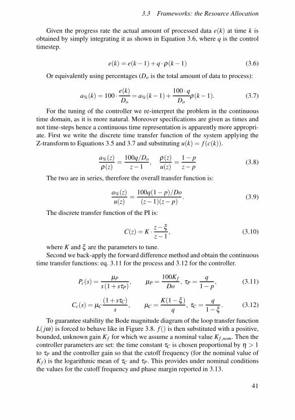
3.3 Frameworks: the Resource Allocation
Given the progress rate the actual amount of processed data e(k) at time k isobtained by simply integrating it as shown in Equation 3.6, where q is the controltimestep.
e(k) = e(k− 1)+ q ·ρ(k− 1) (3.6)
Or equivalently using percentages (Do is the total amount of data to process):
a%(k) = 100 · e(k)
Do
= a%(k− 1)+100 ·q
Do
ρ(k− 1). (3.7)
For the tuning of the controller we re-interpret the problem in the continuoustime domain, as it is more natural. Moreover specifications are given as times andnot time-steps hence a continuous time representation is apparently more appropri-ate. First we write the discrete time transfer function of the system applying theZ-transform to Equations 3.5 and 3.7 and substituting u(k) = f (c(k)).
a%(z)
ρ(z)=
100q/Do
z− 1,
ρ(z)
u(z)=
1− p
z− p(3.8)
The two are in series, therefore the overall transfer function is:
a%(z)
u(z)=
100q(1− p)/Do
(z− 1)(z− p). (3.9)
The discrete transfer function of the PI is:
C(z) = K · z− ξ
z− 1, (3.10)
where K and ξ are the parameters to tune.Second we back-apply the forward difference method and obtain the continuous
time transfer functions: eq. 3.11 for the process and 3.12 for the controller.
Pc(s) =µP
s(1+ sτP), µP =
100K f
Do, τP =
q
1− p, (3.11)
Cc(s) = µC
(1+ sτC)
s, µC =
K(1− ξ )
q, τC =
q
1− ξ. (3.12)
To guarantee stability the Bode magnitude diagram of the loop transfer functionL( jω) is forced to behave like in Figure 3.8. f () is then substituted with a positive,bounded, unknown gain K f for which we assume a nominal value K f ,nom. Then thecontroller parameters are set: the time constant τC is chosen proportional by η > 1to τP and the controller gain so that the cutoff frequency (for the nominal value ofK f ) is the logarithmic mean of τC and τP. This provides under nominal conditionsthe values for the cutoff frequency and phase margin reported in 3.13.
41

Chapter 3. Modelling Big Data Frameworks
0
dB
ω
|L( jω)|
1τP
1τC
= 1ητP
K f
K f ,nom
cutoff frequency ωc
Figure 3.8 Bode magnitude diagram of the required open-loop frequency re-sponse.
ωc =1
η√
τP
, ϕm = arctan(√
η)− arctan(
1√η
)
. (3.13)
Once retrieved the parameters are converted back to the discrete-time domainobtaining the following formulas:
K =Do(1− p)
100qK f√
η, ξ =
η + p− 1η
. (3.14)
With a value of η around 10 – corresponding to φm around 55◦ – as a reasonabledefault the controller behaves satisfactorily provided that q is small enough withrespect to the required completion time. The discrete-time controller in state spaceform reads:
{
xC(k) = xC(k− 1)+ (1− ξ )(a◦%(k− 1)− a%(k− 1))c(k) = KxC(k)+K (a◦%(k)− a%(k))
(3.15)
The number of required cores may transiently assume negative values or exceedthe number of available resources, this plainly means that the control variable issaturated (as we stated also in Section 3.2). Hence the anti-windup must be imple-mented according to eq. 3.16.
xC(k) =c(k)
K− a◦%(k)+ a%(k). (3.16)
Our model captures the xSpark resource allocator activating transitionallocate resources (or de-allocate resources if the control action isnegative) at every control time-step q and computing and allocating the resourcescomputed according to the PI control law.
42
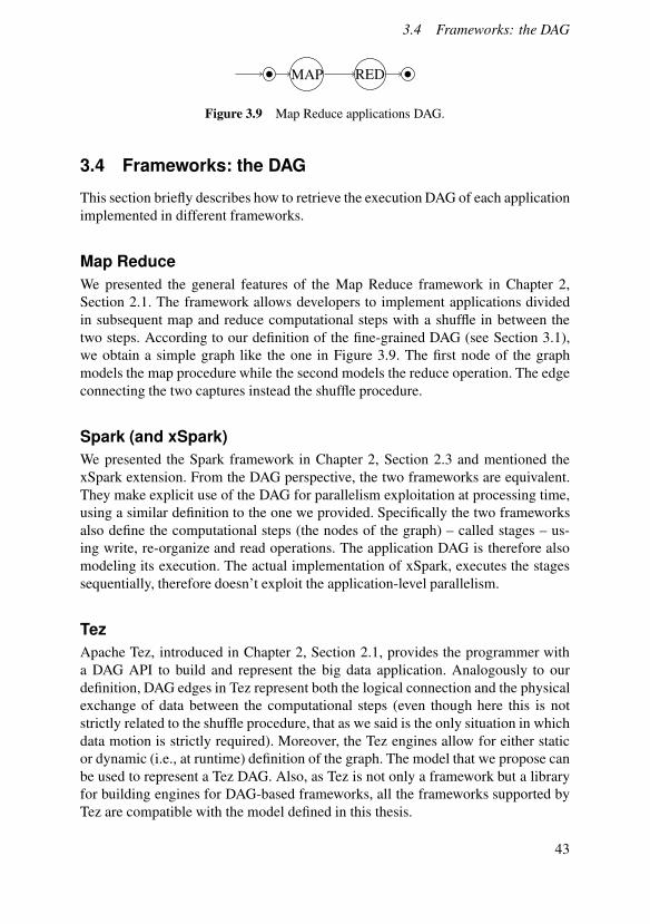
3.4 Frameworks: the DAG
MAP RED
Figure 3.9 Map Reduce applications DAG.
3.4 Frameworks: the DAG
This section briefly describes how to retrieve the execution DAG of each applicationimplemented in different frameworks.
Map Reduce
We presented the general features of the Map Reduce framework in Chapter 2,Section 2.1. The framework allows developers to implement applications dividedin subsequent map and reduce computational steps with a shuffle in between thetwo steps. According to our definition of the fine-grained DAG (see Section 3.1),we obtain a simple graph like the one in Figure 3.9. The first node of the graphmodels the map procedure while the second models the reduce operation. The edgeconnecting the two captures instead the shuffle procedure.
Spark (and xSpark)
We presented the Spark framework in Chapter 2, Section 2.3 and mentioned thexSpark extension. From the DAG perspective, the two frameworks are equivalent.They make explicit use of the DAG for parallelism exploitation at processing time,using a similar definition to the one we provided. Specifically the two frameworksalso define the computational steps (the nodes of the graph) – called stages – us-ing write, re-organize and read operations. The application DAG is therefore alsomodeling its execution. The actual implementation of xSpark, executes the stagessequentially, therefore doesn’t exploit the application-level parallelism.
Tez
Apache Tez, introduced in Chapter 2, Section 2.1, provides the programmer witha DAG API to build and represent the big data application. Analogously to ourdefinition, DAG edges in Tez represent both the logical connection and the physicalexchange of data between the computational steps (even though here this is notstrictly related to the shuffle procedure, that as we said is the only situation in whichdata motion is strictly required). Moreover, the Tez engines allow for either staticor dynamic (i.e., at runtime) definition of the graph. The model that we propose canbe used to represent a Tez DAG. Also, as Tez is not only a framework but a libraryfor building engines for DAG-based frameworks, all the frameworks supported byTez are compatible with the model defined in this thesis.
43

Chapter 3. Modelling Big Data Frameworks
SQL-like Frameworks
As evidenced in [38], SQL-like programming models rely on frameworks that trans-late the query in jobs for other DAG based frameworks, hence validating once morethat the DAG is a power abstraction to capture a general big data application. Forinstance, Hive translates queries in Map Reduce jobs connected as a DAG (in thiscase each of the nodes corresponds to a map and a reduce operation, duplicated tocapture the shuffle that is executed between the two operations). The retrieved DAGis compatible with the proposal of this thesis.
44
4
Implementation and
Validation
Now that we have described the proposed model for big data applications, we canproceed to its implementation and validation. As the final aim of this work is toperform model checking and verify properties of the different applications, we im-plemented the model using the statistical model checker UPPAAL1. This softwaretool serves well for our purpose, because it allows the study of stochastic switchingsystems, and the properties we want to verify are exactly of that nature, like forexample probability distributions and expected values of convenient indicas char-acterizing the evolution of the system. This Chapter first introduces the UPPAALsoftware tool, and then provides some simulations to assess the validity of the UP-PAAL implementation our model.
The aim of model validation in the long term research project to which this the-sis belongs, is mainly to show the validity of our way of reasoning and approachto the big data problem. We want to show that by means of simple “first-principle”abstract models we can recreate the behavior of the applications and the frame-works. As stated in the introduction, we expect that understanding those conceptswill eventually pave the way the implementation of a brand new generation of bigdata frameworks.
4.1 Model Checking and UPPAAL
In the last few years, model checking techniques have been attracting a strong in-terest in both the academic and the industrial world. Those tools are of the “push abutton” kind, meaning that once the model and the properties one wants to verifyare defined and implemented in the formalism of the tool, all one needs to do isto push a button and the software will tell whether or not the system satisfies the
1 http://www.uppaal.org/
45

Chapter 4. Implementation and Validation
property. According to this statement the key ingredients of a model checking toolare:
• An operational formalism to describe the the system to be analyzed,
• A descriptive formalism to describe the properties to be verified,
• An algorithm that can check if a system described using the given operationalformalism satisfies a property defined in the given descriptive formalism.
This is generally called the dual-language approach, as it is based on the ideaof describing the system using an operational language (like automata or timedautomata), and the studied properties using a descriptive language (most frequently,a logic or a temporal logic).
The idea of model checking can be extended allowing a stochastic behavior inthe system description, but this is done at a very high cost, as the model checkingproblem for such systems is undecidable. The approach proposed in the literature toovercome this limitation is called statistical model checking (SMC) [20]. The ideaof SMC is to run a finite number of simulations of the system, and then use resultsfrom statistics to verify properties of the system within some interval of confidence.This classifies SMC between exhaustive model checking and testing. In fact, whileon one side SMC it is not exhaustive as pure model checking, on the other side it ismore expressive and requires by far less memory and time for computing.
UPPAAL is one of those tools. There are several works that present it both froma practical2 and methodological point of view [19] [5]. The tool was extended toimplement also statistical model checking, and such features are presented and ex-plained in [10]. Finally, for what concerns the purely theoretical aspects and foun-dations of the model checking methodology, we refer to [12].
Systems in UPPAAL: the Operational Language
The modeling formalism implemented by UPPAAL SMC is a stochastic extensionof the timed automata [1]. Timed automata extend the basic finite-state automata byintroducing clocks, i.e., variables that generally evolve according to the differentialequation x = 1 where x is the value of the clock. Clocks may influence the behaviorof automata (being part of the transition’s conditions or state’s invariants) and viceversa (transitions may reset or alter the value of clocks). This way, timed automataallow to extend the finite state automata formalism in order to capture their evolutionover time.
A further extension of this formalism is the introduction of stochastic behaviorfor the systems involved. The stochastic extension implemented in UPPAAL re-places the two non-deterministic aspects of timed automata formalism with a prob-abilistic behavior. We now spend a couple of words on this important aspect.
2 https://www.it.uu.se/research/group/darts/uppaal/small_tutorial.pdf
46

4.1 Model Checking and UPPAAL
First, non-deterministic time delays that determine the permanence in a state aresubstituted by probabilistic distributions. Those distributions can be either uniform(for bounded intervals) or exponential (for unbounded intervals)3. For instance, inthe automaton in Figure 4.1, once the condition A for transition activation is satis-fied, there is no information on when the transition will actually be taken: it couldbe immediately or never. Instead, in the stochastic automaton in Figure 4.2, whencondition A is satisfied the system waits for a time determined by an exponentialprobabilistic distribution with initial rate equal to 1. This way the time-delays in-stead of being non-deterministic are refined by probability distributions.
Secondly, when the automaton can chose between two possible transitions, itdoes that accordingly to an (apparently discrete) probabilistic distribution, insteadof non-deterministically. The automaton in Figure 4.3, when condition A is satisfied,will non-deterministically take one of the two transitions and move to states b or c.If say 100 simulations are run, we cannot assume anything about how many timesthe system will move to state b or c. Instead, the automaton represented in Figure 4.4will chose between states b and c according to a discrete probabilistic distributionwhere probability of moving to state b is 0.7 and probability of moving to c is 0.3 .Hence, if 100 simulations are run, the system will approximatively end 70 times inb and 30 in c.
We can use the first kind of statistical modeling to describe time delays that canbe related to communication between nodes (i.e., network efficiency) and in gen-eral to all the phenomena that we cannot (or do not want) to model by means offirst-principle equations. Instead the statistical choice between transitions could beused to model the choice between different possible DAGs for the same applica-tion, hence overcoming the necessity of knowing in advance the control flow of theapplication—see Chapter 3, Section 3.1.
Inside a model, the user can define more than one automaton, and each of themwill evolve concurrently. UPPAAL allows to implement synchronization channelsthat impose simultaneous execution of transitions in different automata. For a tran-sition with a channel to be executed also another process must be ready to execute atransition associated to the same channel. One transition must be marked as receiverand the other as sender. The updates (or in general the code) associated to those isexecuted first on the sender side, and then on the receiver side.
According to the so defined formalism, the system definition results in the endin a network of stochastic timed automata (NSTA).
Properties in UPPAAL: the Descriptive Language
UPPAAL allows to query models in different ways. The queries can regard eitherevaluation of expressions or satisfaction of properties. Expressions are user-definedfunctions that depend on clocks or variables in the system.
3 This constrain is dictated by the possibility of using statistical results for analyzing the results. Thislimitation frequently appears when dealing with our kind of problems.
47

Chapter 4. Implementation and Validation
a
exp λ = 1
bA
Figure 4.1 Non-deterministic Behavior:transition A can be taken or not at any timeinstant (e.g., it could be taken at time i or itcould also never be activated).
a
exp λ = 1
bA
Figure 4.2 Stochastic Behavior: transitionA is taken after a delay determined accord-ing to an exponential distribution with initialrate 1.
a
b
c
A
A
Figure 4.3 Non-deterministic Behavior:when A is satisfied, the choice of the tran-sition to be taken is arbitrary and the systemcould reach either state b or c.
a
b
c
A (0.7)
A (0.3)
Figure 4.4 Stochastic Automaton: when Ais satisfied and the automaton leaves state a,it goes with probability 0.7 to state b andwith probability 0.3 to state c.
Properties are statements about the system expressed with an extension of thetemporal logic, namely the Mixed Interval Temporal Logic (MITL) [2]. This logicallows to express properties over bounded domains for the clocks; this is not bindingfor our analysis, as we want to study applications that execute over a finite time. Theavailable operators are the ones usually implemented in any propositional logic, like“not” ¬ , “and” ∧ , “or” ∨ plus the temporal operators “eventually in the future” ♦
and “always in the future” � with the usual quantifiers “exists” ∃ and “for all” ∀ 4.The available queries for statistical model checking are the following.
• Simulate the defined system : this functionality makes the model evolve fora finite time, defined by the user, and visualizes the value of defined expres-sions. This is not a standard model checking query, but allows the program-mer to get a feedback about whether the system behaves as he expected whenhe implemented it.
4 Note that apparently this is neither an exhaustive nor rigorous definition of the logic implemented byUPPAAL, for such descriptions we refer to the cited works. Here we report the main concepts thatgive an intuition which kind of properties we can (and want) describe.
48
4.2 Model Implementation
• Probability estimation : this query asks UPPAAL to produce an approxima-tion interval [p− ε, p+ ε] for the probability p that a property ψ is verified.p = P(ψ) with confidence (1−α), where ε and α are defined by the user.Hence, given a property, ψ UPPAAL evaluates the probability that ψ is veri-fied.
• Hypothesis testing : this query asks UPPAAL to test the null-hypothesis H :p = PM(ψ)≥ θ against the alternative hypothesis K : p = PM(ψ)< θ . In thiscase, the user is asking to test whether or not the probability that a propertyis verified is bounded by a certain value. UPPAAL asks the user to definealso an execution bound M for the runs that are performed when testing thehypothesis5.
• Probability comparison : this query simply asks UPPAAL to verify amongtwo different properties which has the higher probability of occurring.Bounds must be provided on the simulated time of the queries.
• Expected value : this query asks UPPAAL to estimate the expected value forthe minimum or the maximum of a given expression. This query requires theuser to provide a number of runs to execute for the estimation and, like theprevious queries, a bound on the simulated time.
Extension to Switching Systems
UPPAAL SMC has also been extended to allow the control of the progress rate ofthe clocks. In each state of the modeled automata, the user can impose the progressrate of the clocks using the variables defined inside the model, including the clockvalue itself, thus implementing ordinary differential equations (ODE). This is doneinside the environment “state invariants”, where the user can define progress rateof clocks and properties that the system must satisfy when in this state. In casethose properties are not satisfied and the process cannot evolve without violatingthem, a run-time error will be generated. We use this functionality to implement theprogress of the processing queue, and in general the differential equations inside themodel.
4.2 Model Implementation
In this section we delve into the details of how we implemented the model presentedin Chapter 3 in UPPAAL, for capturing the behavior of the xSpark framework pre-sented in Section 3.3.
A model in UPPAAL is constituted by a set of concurrent processes defined asautomata. For the definition of a model, three environments are available:
5 This bound can be expressed in different ways; suffice here to state that it is generally a bound overthe simulated time.
49
Chapter 4. Implementation and Validation
• An environment for global declarations accessible both in reading and writingby all the processes (data-types, constants, variables, clocks, channels andfunctions),
• A set template definitions of the automata, each with its own environment forlocal definitions accessible only by the automaton itself (constants, variables,clocks and functions),
• An environment for the instantiation of the automata (or equivalently of theprocesses).
Our model defines two automata templates: one for the single computationalstep, and another for implementing an observer that checks whether the applica-tion meets or misses the deadline. We now go through all the environments andtemplates.
Global Declarations
The global declarations include all the informations that are shared among the com-putational steps. Those include:
• The DAG of the application,
• The definition of the cluster on which the application runs,
• Control parameters of the framework,
• The communication channels that allow synchronization of the computationalsteps,
• A couple of commodity functions.
The DAG The DAG is defined using a matrix of booleans called flow_diagram.Each row and each column directly corresponds to a stage of the application, andvice versa: for instance, stage k corresponds to row k and column k. The (i, j) ele-ment of the matrix is true when stage j is a predecessor of stage i, false otherwise.Symmetrically, we can say that (i, j) is true when i is a successor of j. This impliesthat on the generic column j, true values evidence the successors of stage j, whileon generic row i, true values evidence the predecessors of stage i.
Cluster and Allocated Resources The cluster is defined as a set of machines ofgiven and fixed cardinality. Each machine has a fixed number of cores, and eachcore provides a certain (maximum) computational power; the processing rate thatone may desire to govern is ten expressed as jobs (in the broadest sense of theterm) per second per core. The resources, when allocated, are quantized accordingto the machine_quantum variable defined in this environment, as this is a potentialcontrol parameter of the overall application.
50

4.2 Model Implementation
Allocated resourced are described as a vector of integers with as many elementsas the number of stages—a choice that eases the UPPAAL operation, and is consis-tent with the inherently quantized nature of any resource. Specializing to a cluster,each element quantifies the percentage of machines allocated to a given stage ag-gregated with respect to the machines. This means that we cannot distinguish whichmachine is allocated to which stage. It is worth noticing that this would not bea meaningful distinction anyway, under the hypothesis of uniform resources andstages6.
Application Level Control Parameters In the global declarations we find the con-trol parameters related to the application-level control loop(s). Those include theoverall application deadline and the α parameter, that implements the desired mar-gin with respect to the completion of the overall application – as was defined inChapter 3, Section 3.3. A boolean vector for keeping track of the completed nodesis implemented. It is used for the computation of the weight of each stage in theheuristic for stage deadline generation, eq. 3.4.
Channels A matrix of channels with dimensions equal to the number of stages onboth row and columns is implemented. As channels impose simultaneous executionof transitions in different processes (automata), they come into play when synchro-nization between stages is required. Channel (i, j) is used when stage j (marked assender) wants to communicate with stage i (marked as receiver), we will get back onthis when describing the behavior of the single computational step in Sections 4.2and 4.2.
Functions The commodity functions implemented here are two. One returns thenumber of missing stages, information required in the deadline loop that implementsthe heuristic shown in Chapter 3, Section 3.3. The second one receives as input adouble and returns the smallest integer that is bigger than the input. This latterfunction is used when values of the kind of double are assigned to int variables.
Computational Step Template
The automaton template of the single stage implemented in UPPAAL is shown inFigure 4.5. As we can see, there is here one main difference with respect to the theo-retical one presented in Figure 3.5: the transition leaving the processing state anddefining a self-loop. This transition implements the resource allocator. In fact, re-source allocation is activated only in this state of the stage automaton, and in xSparkthe stage-level control of each computational step is independent of the controls ofthe other stages. For this reason there is no need for a parallel process represent-ing it, and doing so would increase the complexity without implementing specificfunctionalities. Still, all the stages allocate resources from the same pool (the global
6 This is a necessary hypothesis as we want the framework model to be agnostic with respect to thisinformation. The resource allocation logic (i.e. the control) should guarantee adaptation with respectto those variabilities or, using control-theoretical terms, should reject those disturbances.
51

Chapter 4. Implementation and Validation
Figure 4.5 Stage automaton as implemented in UPPAAL.
variable), hence the representation of the “competition” among parallel stages forthe resources is preserved.
Stage Declarations As we said, we can declare variables that live within the scopeof the single process. This means that those variables are accessible only by theprocess they are associated to. Moreover when allocating the single stage we candefine some input parameters for the process. For the stage template those are:
• The integer id that is a univocal identifier for the stage,
• The integer initial defining the volume of input data that do not come frompredecessors7,
• The fraction_factor defining the ratio between volume of input data andoutput data8,
7 This is used for the starting stages, that do not receive the data from other stages but process the rawinput of the application.
8 This depends on the actual data and operations that are being executed so we cannot provide a generalmodel for it. Here we define it as an input in order to have the same data volumes of the applicationexecutions of which we have data. In the general case where we do not have this information; it can
52

4.2 Model Implementation
• The weight parameter w corresponding to the w(sk) parameter defined inChapter 3, eq. 3.3.
In our model the variables of the stage template can be divided in two groups:one comprising the variables that define the state of the stage computation, related tothe progress of processing itself, the second with the variables related to the control,hence defined by the framework.
In the first group we find:
• The variables input_dim and processing_bound that define the volume ofthe data set to process,
• Two boolean vectors received_predecessorsand inofrmed_successorsthat respectively keep track of which predecessors have synchronized at thebeginning of the computation and which successors have synchronized at theend,
• The clock queue_processing that is the “core” variable of the stage: it de-scribes the amount of processed data (i.e. the e variable in eq. 3.1 defined inSection 3.2),
• The constant pr_pole defining the pole of the resource allocation dynamicsdescribed in Chapter 3, eq. 3.5.
Instead the variables related to the control are:
• The constants gamma and beta implementing respectively the γ parameterdefined in Chapter 3, Section 3.3 and the β parameter used in eq. 3.4,
• The stage deadline and the weight parameter (corresponding to theweight(sk) used in eq. 3.2) both computed at the beginning of the process-ing,
• The variable reference_rate computed according to the deadline and γparameters,
• The variable start_time used for storing the time at which the processingof the stage started,
• The variable ci_old implementing the state variable of the controller,
• The clock t_ctrl and constant q used for implementing the control time step(the constant corresponds to the q defined in Chapter 3, Section 3.3),
be statistically modeled by substituting a parameter computed at the end of the processing accordingto some probabilistic distribution.
53

Chapter 4. Implementation and Validation
• The variables estimated_cores, stage_saturation and the constantoverscale used by xSpark for bounding the total amount of resources avail-able for the single stage.
We now go through each of the states and transitions of the template.
Waiting for Synchronization This state implements the state described in Sec-tion 3.2. Here no data processing and no control is happening, so the rate of theclocks t_ctrl and queue_processing are fixed at zero (defined in the invariantsof the state).
In this state the automaton may activate two transitions with mutually exclu-sive conditions. One of those is described by the self-loop for synchronizing withthe predecessors, it is in fact associated to the channel update_input[id][j] andcan be taken when condition not check_predecessors() is valid. The functioncheck_predecessors() returns a boolean value that is true when all the prede-cessors have terminated and synchronized with the present node, false otherwise9.When the transition is taken, the function update_input_dim() is executed: thisfunction updates the variable received_predecessors and increments the vari-able input_dim reading the value of the global meta-variable10 total_update.The variable was in fact first updated by the predecessor (see Section 4.2), exploit-ing the fact that the transition code is first executed by the sender and then by thereceiver.
When all the predecessors have terminated and synchronized with the givenstage, the output of function check_predecessors() returns true, hence the au-tomaton may take the transition to the Processing state. When taking this tran-sitions different functions are executed. The processing_bound variable is up-dated summing the input dimension received from the predecessors and the inputof the template initial. Function compute_stage_deadline() computes thestage deadline, the reference rate, the estimated cores and the stage saturation: ingeneral we can say that this function initializes the control of the stage. Functioninitialize_resources initializes the allocated resources to the node accordingto the estimated required cores (also the state of the controller is initialized accord-ingly). Finally, the function update_processing_rate() computes the process-ing rate reading the allocated resources and implementing eq. 3.5.
Processing As defined in Section 3.2, in this state the actual processing of data ismodeled. In fact the rate of the clock queue_processing is set equal to variablepr that was previously initialized by the function update_processing_rate().
9 The function simply compares the vector variable received_predecessors defined before withthe predecessors defined by the DAG.
10 A meta-variable is a variable that is not part of the state hence the programmer cannot rely on it havingthe same value across the execution of different transitions. When possible it is used to reduce thestate-space of the implemented system and improve efficiency of model checking.
54
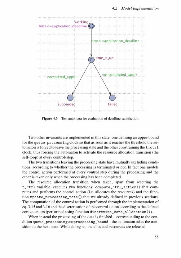
4.2 Model Implementation
Figure 4.6 Test automata for evaluation of deadline satisfaction.
Two other invariants are implemented in this state: one defining an upper-boundfor the queue_processing clock so that as soon as it reaches the threshold the au-tomaton is forced to leave the processing state and the other constraining the t_ctrlclock, thus forcing the automaton to activate the resource allocation transition (theself-loop) at every control-step.
The two transitions leaving the processing state have mutually excluding condi-tions, according to whether the processing is terminated or not. In fact one modelsthe control action performed at every control step during the processing and theother is taken only when the processing has been completed.
The resource allocation transition when taken, apart from resetting thet_ctrl variable, executes two functions: compute_ctrl_action() that com-putes and performs the control action (i.e. allocates the resources) and the func-tion update_processing_rate() that we already defined in previous sections.The computation of the control action is performed through the implementation ofeq. 3.15 and 3.16 and the discretization of the control action according to the definedcore quantum (performed using function discretize_core_allocation()).
When instead the processing of the data is finished – corresponding to the con-dition queue_processing>= processing_bound– the automaton takes the tran-sition to the next state. While doing so, the allocated resources are released.
55

Chapter 4. Implementation and Validation
Output This state is the dual of the initial one. Here the process is ready to syn-chronize and communicate to the successors its output data. This is done executingthe transition that defines a self-loop synchronized with the one in the initial stateexecuted by the successor.
The value assigned to the total_update variable – that will be readby the successor – is the processing_bound times the fraction_factor
this defines the volume of output data. This is done until the functionall_successors_informed() that compares the vectors of successors (takenfrom the matrix defining the DAG) and the vector of informed successors returnstrue. At this point the other transition to the end state is taken and the stage updatesits execution state in the global variable completed_nodes.
Deadline Observer
A common way to define properties in model checking, is the usage of test-
automata [6]. This idea is mainly motivated by the desire of avoiding expressingproperties of the systems with the logic, and instead use simpler automata that evi-dently enjoy the said properties. Doing so is not by itself more powerful than usingthe logic (in the sense that one cannot express more properties), but can be easierto understand for the user. More precisely, the approach is to define an automatoninside the model and make it behave in such a way that it detects (in the sense that itchanges its state) the occurrence of specific events or sequences of events. Then thequery can be easily expressed on the final state of the defined automaton. Propertiesexpressed this way frequently are of the kind of bounded liveness, but this is notexclusive.
In this work, we use this idea for checking whether an application meets ormisses the deadline. This is a trivial task, as the deadline is defined as a globalvariable and it is therefore accessible from all processes, the deadline observerincluded. This simple automaton is shown in Figure 4.6. The automaton doesnothing until the time reaches the deadline, at this moment the invariant time <application_deadline of the initial state is not valid anymore, and the processis forced to leave the state. This cannot happen earlier, as the transition that leavesthis state has the condition time >= application_deadline. The next state, theone called time_is_up is marked as committed, this means that when in this statethe process is forced to leave it without any delay. The two transitions leaving thisintermediate state have mutually excluding conditions about whether the applicationhas finished running or not. In the first case the application ends in state succeeded,otherwise in state failed.
Using this automaton, we can simply ask the model checker about the proba-bility of runs such that the deadline observer ends in the state failed and directlyretrieve the probability the application meeting the deadline or not.
56
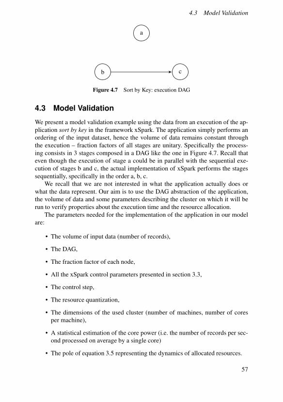
4.3 Model Validation
a
b c
Figure 4.7 Sort by Key: execution DAG
4.3 Model Validation
We present a model validation example using the data from an execution of the ap-plication sort by key in the framework xSpark. The application simply performs anordering of the input dataset, hence the volume of data remains constant throughthe execution – fraction factors of all stages are unitary. Specifically the process-ing consists in 3 stages composed in a DAG like the one in Figure 4.7. Recall thateven though the execution of stage a could be in parallel with the sequential exe-cution of stages b and c, the actual implementation of xSpark performs the stagessequentially, specifically in the order a, b, c.
We recall that we are not interested in what the application actually does orwhat the data represent. Our aim is to use the DAG abstraction of the application,the volume of data and some parameters describing the cluster on which it will berun to verify properties about the execution time and the resource allocation.
The parameters needed for the implementation of the application in our modelare:
• The volume of input data (number of records),
• The DAG,
• The fraction factor of each node,
• All the xSpark control parameters presented in section 3.3,
• The control step,
• The resource quantization,
• The dimensions of the used cluster (number of machines, number of coresper machine),
• A statistical estimation of the core power (i.e. the number of records per sec-ond processed on average by a single core)
• The pole of equation 3.5 representing the dynamics of allocated resources.
57
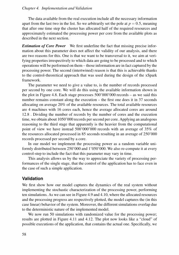
Chapter 4. Implementation and Validation
The data available from the real execution include all the necessary informationapart from the last two in the list. So we arbitrarily set the pole at p = 0.5, meaningthat after one time step the cluster has allocated half of the required resources andapproximately estimated the processing power per core from the available plots asdescribed in the next section.
Estimation of Core Power We first underline the fact that missing precise infor-mation about this parameter does not affect the validity of our analysis, and thereare two reasons for this. One is that we want to be transversal to it, we aim at veri-fying properties irrespectively to which data are going to be processed and to whichoperations will be performed on them – those information are in fact captured by theprocessing power. The second (intertwined) reason is that this is achievable thanksto the control-theoretical approach that was used during the design of the xSparkframework.
The parameter we need to give a value to, is the number of records processedper second by one core. We will do this using the available information shown inthe plot in Figure 4.8. Each stage processes 500’000’000 records – as we said thisnumber remains constant along the execution – the first one does it in 37 secondsallocating on average 20% of the available resources. The total available resourcesare 4 machines with 16 cores each, hence the average allocated cores are around12.8 . Dividing the number of records by the number of cores and the executiontime, we obtain about 1050’000 records per second per core. Applying an analogousreasoning to the third stage that apparently is the heavier from the computationalpoint of view we have instead 500’000’000 records with an average of 35% ofthe resources allocated processed in 85 seconds resulting in an average of 250’000records processed per second by a core.
In our model we implement the processing power as a random variable uni-formly distributed between 250’000 and 1’050’000. We also re-compute it at everycontrol-step to include the fact that this parameter may vary in time.
This analysis allows us by the way to appreciate the variety of processing per-formances of the single stage, that the control of the application has to face even inthe case of such a simple application.
Validation
We first show how our model captures the dynamics of the real system withoutimplementing the stochastic characterization of the processing power, performingten simulations. As we can see in Figure 4.9 and 4.10, where the allocated resourcesand the processing progress are respectively plotted, the model captures the (in thiscase linear) behavior of the system. Moreover, the different simulations overlap dueto the deterministic nature of the implemented model.
We now run 50 simulations with randomized value for the processing power;results are plotted in Figure 4.11 and 4.12. The plot now looks like a “cloud” ofpossible executions of the application, that contains the actual one. Specifically, we
58

4.3 Model Validation
Figure 4.8 Execution progress and resource allocation profiles in the execution ofsort by key application.
0 20 40 60 80 100 120 140 160 180 2000
20
40
60
80
100
Time [s]
Resource%
Stage 0Stage 1Stage 2
Figure 4.9 Non stochastic simulation of the implemented model: plot of allocatedresources.
0 20 40 60 80 100 120 140 160 180 2000
20
40
60
80
100
Time [s]
Record
%
Stage 0Stage 1Stage 2
Figure 4.10 Non stochastic simulation of the implemented model: plot processingprogress per stage.
59
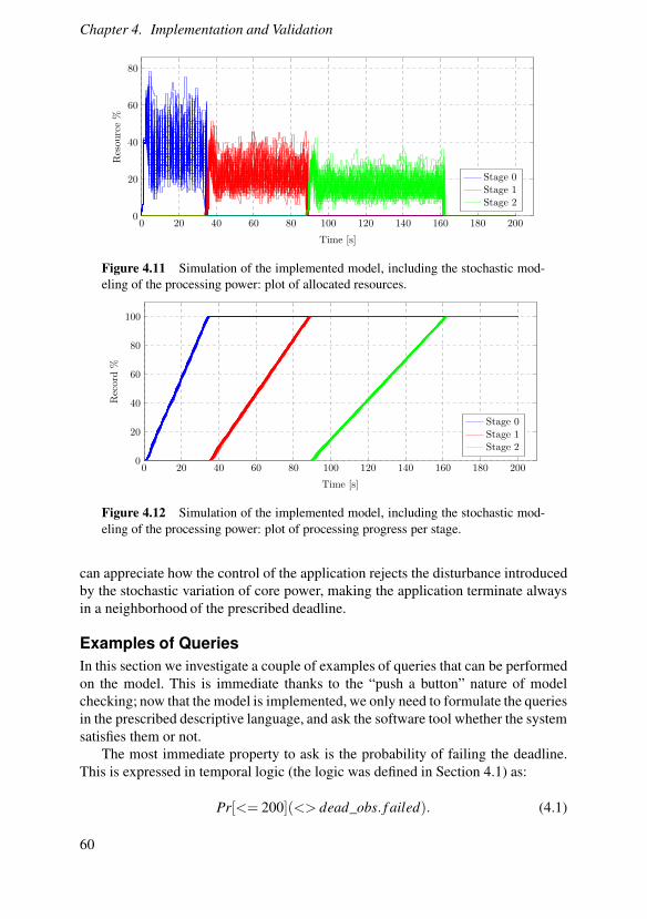
Chapter 4. Implementation and Validation
0 20 40 60 80 100 120 140 160 180 2000
20
40
60
80
Time [s]
Resource%
Stage 0Stage 1Stage 2
Figure 4.11 Simulation of the implemented model, including the stochastic mod-eling of the processing power: plot of allocated resources.
0 20 40 60 80 100 120 140 160 180 2000
20
40
60
80
100
Time [s]
Record
%
Stage 0Stage 1Stage 2
Figure 4.12 Simulation of the implemented model, including the stochastic mod-eling of the processing power: plot of processing progress per stage.
can appreciate how the control of the application rejects the disturbance introducedby the stochastic variation of core power, making the application terminate alwaysin a neighborhood of the prescribed deadline.
Examples of Queries
In this section we investigate a couple of examples of queries that can be performedon the model. This is immediate thanks to the “push a button” nature of modelchecking; now that the model is implemented, we only need to formulate the queriesin the prescribed descriptive language, and ask the software tool whether the systemsatisfies them or not.
The most immediate property to ask is the probability of failing the deadline.This is expressed in temporal logic (the logic was defined in Section 4.1) as:
Pr[<= 200](<> dead_obs. f ailed). (4.1)
60
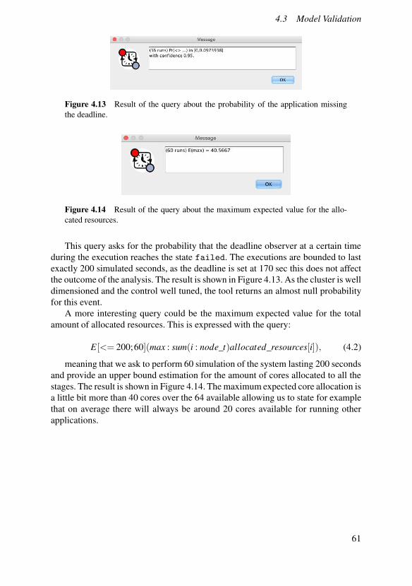
4.3 Model Validation
Figure 4.13 Result of the query about the probability of the application missingthe deadline.
Figure 4.14 Result of the query about the maximum expected value for the allo-cated resources.
This query asks for the probability that the deadline observer at a certain timeduring the execution reaches the state failed. The executions are bounded to lastexactly 200 simulated seconds, as the deadline is set at 170 sec this does not affectthe outcome of the analysis. The result is shown in Figure 4.13. As the cluster is welldimensioned and the control well tuned, the tool returns an almost null probabilityfor this event.
A more interesting query could be the maximum expected value for the totalamount of allocated resources. This is expressed with the query:
E[<= 200;60](max : sum(i : node_t)allocated_resources[i]), (4.2)
meaning that we ask to perform 60 simulation of the system lasting 200 secondsand provide an upper bound estimation for the amount of cores allocated to all thestages. The result is shown in Figure 4.14. The maximum expected core allocation isa little bit more than 40 cores over the 64 available allowing us to state for examplethat on average there will always be around 20 cores available for running otherapplications.
61
5
Model Extensions
The model introduced in Chapter 3 was shown to be able of reproducing applicationdata precisely enough, and therefore to be suitable for verifying the properties ofinterest via model checking applied to the simulator of an application instead of theapplication itself.
However, although the model fullfils the goal set for this thesis, it also con-tains some quite relevant simplifications, that it may be interesting to relax in aview to applying the devised modeling principles to a more fine-grained analysis.The purpose of this chapter is to propose an extended model to overcome the saidsimplifications.
5.1 Limits to Overcome
The limitations of the model proposed in Chapter 3 – hereinafter the basic model,as opposed to the extended one presented in the following – are basically two.
• The operation of a stage is represented monolithically, without describing itspartition into the elaboration and the reading/writing of data.
• The processing of data proceeds at a speed proportional (among other factorssome of which unpredictable) to the allocated resources, but this fact is repre-sented as if there were only one elaboration unit with more or less resources,not evidencing the presence of several units possibly operating in parallel.
To avoid possible confusions, it is worth specifying that in fact the basic modeldoes represent parallelism, but only at the level of the DAG, i.e., in how the programrealizing the application is written. The level of parallelism related to the singleoperations, instead, is not modeled, since – adopting for a moment the Spark jargon– there is no evidence of the executors spawned in parallel, on different cores, tocarry out a stage.
Indeed, for several analysis activities, the basic model is more than enough. Forexample, when aiming at the first-cut sizing of an elaboration architecture, one may
62

5.2 The Extended Model
not yet have precise enough an idea of how many units will be required, and thusdesire to obtain that number exactly from the simulation of a model in the basicform. Or, ideas may not be yet clear on the communication and storage part of thearchitecture, and therefore one may decide to just give a rough quantification of theconsequent time overhead, and include it in that of the processing time.
The basic model, on the other hand, clearly reveals its shortcomings when thepurpose of the simulation and checking activity is not sizing an architecture, whichhas to be done in a cautious manner anyway, but rather providing reliable and pre-cise enough estimates – possibly based also on the profiling of convenient bench-mark applications – of the data processing times really observed at runtime.
5.2 The Extended Model
In the basic model a stage is viewed as a single entity that has to process a givenamount of data. The processing speed is governed by allotting this entity more orless elaboration units, which is viewed as equivalently providing a single more orless powerful one. There is no evidence of the physical means by which this isrealized.
In the extended model, when a stage starts, the data to be processed is splitinto a number of subsets. The processing of one of these subsets, that can takeplace in parallel with others, is called a task. The processing speed of the stage isgoverned by spawning more or less executors, that can be thought here as sequentialelaboration units taking care of one task, thereby allowing more or less tasks to runin parallel.
In both cases the number of available elaboration units is clearly limited, as thecluster has a finite number of cores, whence the allocation problem. However, theextended model can for example describe the situation in which some executorscome to transiently reducing their operating speed, which is apparently impossiblefor the basic one.
Coming to the breakdown of the data elaboration, in the basic model there is no“data transfer” if not from a stage to the downstream ones—in other words, onlywhen locality is violated. In the extended model we conversely need to account forthe time spent in attributing their subsets to the stage tasks. We therefore separatethe reading of data from its elaboration, describing the former as a delay. The sameis not required for the writing operation, as this takes place contextually with theelaboration itself. In fact, as soon as part of the output is produced, this is directlywritten to the application file system, which affects the overall processing time onlyto a nearly negligible extent.
For the sake of completeness, one may argue that even though the writing pro-cedure itself does not require a relevant time with respect to the overall computationtime, it may load the network, and thus indirectly affect the reading time. However,in this respect, a couple of factors must be considered: first, differently from the
63
Chapter 5. Model Extensions
reading procedure, the writing one can be forced to take place on a cluster nodeclose to the one that processes the data or even on the same node, resulting in amarginal load for the network: second, the volume of output data is usually smallerthan the volume of input data—at least, on an average basis.
Despite the remarks just made. one could still not desire to neglect the writingtime. The extended model can be very easily adapted to allow this, but the matter isleft to future works.
The extended model is composed of a state machine, representing the operat-ing states traversed by the elaboration units. This state machine governs the evolu-tion of a continuous-time dynamic system describing the units themselves. Differ-ently from the basic model, as the number of active units can vary, the order of thecontinuous-time part of the model can vary as well, making the extended model ahybrid – not switching – dynamic system.
5.3 Implementation of the Extended Model
The extended model, with respect the basic one, changes the way the processing ofdata is described. For this reason the differences between the two are confined tohow the processing of data is captured.
The model extension includes the deploying of tasks that process the data inparallel. To implement this, we use an UPPAAL functionality that allows to dynamicallocate (or using UPPAAL jargon, spawn) of processes within the model, hence tocapture an hybrid system (as it does not require to know in advance how manyprocesses will be launched).
From the implementation point of view, there are two main differences: the be-havior of the stage in the processing state is different, and the dynamic template ofthe executors is introduced. We now present the introduced features.
Stage Implementation Differences Figures 5.1 and 5.2 show the stage automatonin the extended model: as we can see, the behavior differs from the basic modelonly in the processing state. When in this state, if the processing is not terminated,it takes a transition at every control step – analogously to the basic model – andmoves to another state named spawn tasks. When taking this transition the controlaction – i.e., the number of resources (executors) to allocate – is computed: forreasons explained in the next section, in this case we allocate only a constant numberof those. The update of the pr variable instead is implemented here to make thismodel comparable to the basic one, the way it affects the processing will be shownwhen describing the executor template. The state spawn executors is marked ascommitted that means that when in this state no delay is allowed and the system mustimmediately take a transition exiting the state. In this state the automaton cycles onthe self-loop transition and once at a time allocates an executor. This is done untileither the overall resources are saturated or the number of executors matches thenumber requested by the controller. Then, the process takes the transition back to
64

5.3 Implementation of the Extended Model
Figure 5.1 Stage automaton of the extended model implemented in UPPAAL
Figure 5.2 Zoom on the processing phase in the stage automaton of the extendedmodel
the processing state. When eventually a controller is implemented, the anti wind-upprocedure must be performed in this transition, as only at this moment the actualamount of allocated resources is known.
Executor Template The implementation of the template of an executor is shownin figure 5.3. This automaton is supposed to capture the sequence of procedures thatare involved in the processing of a single task. When spawned, the automaton is ina initial “committed” state, which it is forced to leave immediately. The automa-ton hence moves to the reading state, using a transition that computes the readingdelay—i.e., the time it will have to wait before being able to move to the process-ing state. As at the moment we do not have any model for the reading delay, hencehere we made the hypothesis of a delay that is constituted by a constant term plusa linear function of the number of deployed executors. This idea should be verifiedusing real data from adequately instrumented applications, or by trying to (finely)model the “inner-physics” of the network. When the process leaves the reading state
65

Chapter 5. Model Extensions
Figure 5.3 Executor Template implemented in UPPAAL
it moves to the one modeling the processing. The processing delay is implementedin a slightly different manner: the threshold is constant and the clock rate varies.The rate is determined at every control step as it was in the basic model in orderto achieve comparability between the two. Also the variability is properly chosento emulate the previous one, how this is done is described in section 5.4. Once theprocessing is completed, the executor increases by one the number of overall com-pleted tasks in the stage, and start to process another task, if instead before thishappens the amount of allocated resources is reduced the executor deallocates itselfusing function exit().
We chose to implement only the reading and writing procedures, but we can seethat the model could be extended introducing for instance another state capturingother procedures.
5.4 Testing the Extended Model
In this section we briefly present two tests. The first one is aimed at showing thatthe extended model, although different from the basic model as for its implemen-tation, does in fact comprehend the simpler model. This is achieved by simulatingan application with the basic model and then with the extended one, but allowingfor only one elaboration unit in parallel, and setting the data reading delay to zero.Consistency of the two models is verified as for both the execution traces, and theprobabilistic assessment of a property.
The second test is conversely aimed at evidencing the additional representation
66

5.4 Testing the Extended Model
capabilities of the extended model. This is obtained by starting from the same sit-uation just described, and showing how the property assessment is affected by theintroduction of a data reading delay.
Since the aim of both test is to assess the descriptive capabilities of the models,no control is involved—hence we “disable” the controller and impose a constantamount of allocated resources.
Test one – Consistency
The aim of this test is to verify that the extended model discussed in Section 5.2is able to capture the physical behavior described by the basic model presented inChapter 3. We achieve this objective by presenting one simulation with equivalentparameters for both models—the core power for the basic model (as defined insection 4.3), and the equivalent processing time per task in the extended model. Ourresults show that, despite the more complex dynamics introduced in the extendedmodel and the uncertainty encoded in the mentioned parameters, the results in termsof execution times are comparable. In the extended model, reading delays are set tozero, in order to match the basic model behavior.
Our simulations involve the same application presented in 4.3, composed ofthree stages, each with a fraction factor of 1, i.e., preserving the total amount ofrecords to process. The application is given 500M input records that have to beprocessed by the three stages sequentially. Both in the extended model and in thebasic one, the application is given 32 cores. This is simply a number for the basicmodel, while in the extended model case, having access to 32 cores implies that theapplication can run 32 tasks in parallel. Each of the tasks of the extended model isgiven 500K records to process, therefore a total number of 1000 tasks is to be runfor completion.
For each second of the simulation, in both models, the stochastic parametersare updated from a uniform random distribution. In the case of the basic model,the core power (the amount of record processed in a second per core) is uniformlydistributed between 350 and 850. For the extended model, the stochastic behavior isencoded as the number of tasks completed per second per core. To obtain the samerandom distribution, we therefore utilize the same random variable parameters anddivide them by the number of records per task (500K).
[
record
s · core
]
·[
task
record
]
=
[
task
s · core
]
(5.1)
Figures 5.4 and 5.5 show respectively the results of 50 different simulationsof the basic and extended models. As can be seen, the completion times of firststage are almost identical, the range being between 25 and 30 seconds. For thesecond and third stage, differences become slightly more evident – justifying tosome extent the necessity of a model that includes more details providing resultsof finer granularity. Nevertheless, it is worth noticing that the basic model, despite
67

Chapter 5. Model Extensions
0 10 20 30 40 50 60 70 80 90 100 1100
100000
200000
300000
400000
500000
Time [s]
Record
·1000
Stage 0Stage 1Stage 2
Figure 5.4 Basic model, no delay.
0 10 20 30 40 50 60 70 80 90 100 1100
100000
200000
300000
400000
500000
Time [s]
Record
·1000
Stage 0Stage 1Stage 2
Figure 5.5 Extended model, no delay.
being notably simpler, catches the results of the extended one by far less than anorder of magnitude, therefore proving to be well suitable for a first cut evaluation.
For example, observing Figure 5.5 and in particular the curves for the beginningof the stage 1 execution and the progress rate of stage 2, one can notice the quan-tization of the progress of the computation. This models very well the availabilityof measurement and information within the big data framework – it is in fact im-possible to properly be informed about the progress of the execution if not for thecompletion time of tasks. This is also evident in the execution traces from the runshown in Figure 4.8. The extended model better capture the nature of the feedbacksignal, therefore being more suited for fine grain evaluation of the performance ofthe big data framework together with the computation infrastructure.
Test two – Extension
The aim of this second test is to show the characteristics of the extended model (andof the execution on the real hardware) that are not captured by the basic model. Weachieve this by setting a nonzero reading delay and verifying the performance degra-
68

5.4 Testing the Extended Model
0 10 20 30 40 50 60 70 80 90 100 1100
100000
200000
300000
400000
500000
Time [s]
Record
·1000
Stage 0Stage 1Stage 2
Figure 5.6 Extended model, delay
dation (longer execution times). Specifically, the model factors in a constant delayfor the setup of the reading channel and a delay that is proportional to the numberof the running tasks. This second term allows the extended model to capture an in-crease in network load – which results in lower reading speed – due to concurrency.All the other parameters (computing speed, allocated resources, etc.) are kept con-stant. Figure 5.6 shows the simulations obtained with the extended models and adelay of 0.1s for the channel setup and an additional delay of 0.0001s per runningtask. The figure displays, in fact, longer execution times for each of the stages andtherefore a longer completion time for the overall application.
69

6
Conclusion and Future
Work
The aim of this work was to provide a first-principle modeling approach to big dataapplications and frameworks. The main motivation for this is to make model check-ing feasible in the addressed context. Specifically, once the model is proven able torepresent the characteristics of the evolution of a big data application informativelyenough, it is possible to carry out model checking operation on the simulator of theapplication instead of the application itself. Since the former is far less complex andcomputationally intensive, the advantages are apparent. Indeed, important proper-ties can be assessed at a very small fraction of the cost, and model checking can beconsidered even for applications that in the absence of a suitable simulation modelwould simply be intractable.
Once the model has been proposed, including some relevant extensions to thebasic principles, and tests have been presented to demonstrate its adequacy to theintended purpose, it is now the time to take a wider perspective.
In fact, this thesis is part of a long term research project, the major aim of whichis not only to model and simulate the existing technology, but ultimately to deviseand realize a brand new generation of big data frameworks, where the system- andcontrol-theoretical attitude here just introduced is brought to guide the entire design.As a result, several research directions are open, that can be broadly classified inthree sets:
• Application modeling,
• Architecture/hardware modeling,
• Framework design and realization.
The first activity set is basically the continuation of the analysis carried out inthis work, in a view to exploiting the devised abstractions to improve the softwarearchitecture of the applications.
70

6.1 Application Modeling
The second set is conversely a step ahead with respect to this work. Once thesoftware-related abstractions are assessed, the idea is to extend the modeling strat-egy to the hardware that executes the application, determining and adopting theconvenient level of descriptive detail. This is surely an ambitious objective, as theinvolved architectures are typically cloud-based.
The third set, finally, amounts to turn methodological results on modeling, sim-ulation and control, into engineering practices for the control-based design of bigdata frameworks.
Despite the activities just mentioned are nowadays largely to be defined, theexperience gathered in this work allows to spend some final words at least on thefirst two, thereby sketching out, with the detail feasible to date, future activities inthis context.
6.1 Application Modeling
From this viewpoint, the first problem to address is how to generate the DAG fromthe code of an application automatically, and for different frameworks. On one handthis has an operational importance, as it avoids to input the same information twiceand reduces the possibility of modeling errors. On the other hand, and more impor-tant, the solution of this problem will provide further support to the generality andthe descriptive capabilities of the proposed modeling paradigm.
A second relevant issue is whether or not, and in the affirmative case how, it ispossible to manipulate a DAG so as to generate another one, functionally equivalentbut with some optimality properties. Besides its obvious usefulness, a solution tothis problem would inherently allow to define a “theoretically optimal” performancefor the application, possibly – and hopefully – independent of the dataset and thecluster.
As a result of addressing the points above, one should be able to define a pro-gramming model (or extend existing ones) so that the DAG can be generated bythe compiler instead of by the programmer (in an implicit way), and automaticallycompleted with the information required to set up and run its simulation (at both thebasic and the extended level) and model checking.
6.2 Architecture/Hardware Modeling
This activity will aim at completing the description of the application with that ofthe hosting computing machinery (especially in terms of network access and datamanagement), in the broadest sense of the term. A significant effort will be requiredto relate this work to the huge existing corpus of computing systems modeling,fulfilling however the specific needs – evidenced in the previous chapters – of thebig data context.
71

Chapter 6. Conclusion and Future Work
The expected results is that quantities relative to the file system, the network andthe computing nodes, instead of being provided – normally in a conservative manner– by the user, can be obtained automatically. Solving this problem would makeit possible to rapidly and systematically evaluate an application and the hostingarchitecture at the same time, and therefore to pave the way toward the realizationof new big data frameworks that take advantage right form the start of their design
of the control-theoretical approach adopted here.
72

Bibliography
[1] R. Alur and D. L. Dill. “A theory of timed automata”. Theor. Comput.
Sci. 126:2 (1994), pp. 183–235. ISSN: 0304-3975. DOI: 10.1016/0304-3975(94) 90010- 8. URL: http: / / dx . doi . org / 10 . 1016/ 0304-3975(94)90010-8.
[2] R. Alur, T. Feder, and T. A. Henzinger. “The benefits of relaxing punctual-ity”. J. ACM 43:1 (1996), pp. 116–146. ISSN: 0004-5411. DOI: 10.1145/227595 . 227602. URL: http : / / doi . acm . org / 10 . 1145 / 227595 .227602.
[3] K.-E. Årzén, A. Robertsson, D. Henriksson, M. Johansson, H. Hjalmarsson,and K. H. Johansson. “Conclusions of the artist2 roadmap on control of com-puting systems”. SIGBED Rev. 3:3 (2006), pp. 11–20. ISSN: 1551-3688. DOI:10.1145/1164050.1164053. URL: http://doi.acm.org/10.1145/1164050.1164053.
[4] L. Baresi, S. Guinea, A. Leva, and G. Quattrocchi. “A discrete-time feedbackcontroller for containerized cloud applications”. In: Proceedings of the 2016
24th ACM SIGSOFT International Symposium on Foundations of Software
Engineering. FSE 2016. ACM, Seattle, WA, USA, 2016, pp. 217–228. ISBN:978-1-4503-4218-6. DOI: 10.1145/2950290.2950328. URL: http://doi.acm.org/10.1145/2950290.2950328.
[5] G. Behrmann, A. David, and K. G. Larsen. “A tutorial on uppaal”. In:M. Bernardo et al. (Eds.). Formal Methods for the Design of Real-Time
Systems: International School on Formal Methods for the Design of Com-
puter, Communication, and Software Systems, Bertinora, Italy, September
13-18, 2004, Revised Lectures. Springer Berlin Heidelberg, Berlin, Heidel-berg, 2004, pp. 200–236.
[6] J. Bengtsson, K. Larsen, F. Larsson, P. Pettersson, and W. Yi. “Up-paal—a tool suite for automatic verification of real-time systems”. In:Proceedings of the DIMACS/SYCON Workshop on Hybrid Systems III : Ver-
ification and Control: Verification and Control. Springer-Verlag New York,
73
Bibliography
Inc., New Brunswick, NeW Jersey, USA, 1996, pp. 232–243. ISBN: 3-540-61155-X. URL: http://dl.acm.org/citation.cfm?id=239587.239611.
[7] V. Borkar, M. Carey, R. Grover, N. Onose, and R. Vernica. “Hyracks: a flexi-ble and extensible foundation for data-intensive computing”. In: Proceedings
of the 2011 IEEE 27th International Conference on Data Engineering. ICDE’11. IEEE Computer Society, Washington, DC, USA, 2011, pp. 1151–1162.ISBN: 978-1-4244-8959-6. DOI: 10 . 1109 / ICDE . 2011 . 5767921. URL:http://dx.doi.org/10.1109/ICDE.2011.5767921.
[8] T. C. Bressoud and Q. Tang. “Analysis, modeling, and simulation of hadoopYARN mapreduce”. In: 2016 IEEE 22nd International Conference on Paral-
lel and Distributed Systems (ICPADS). 2016, pp. 980–988. DOI: 10.1109/ICPADS.2016.0131.
[9] Clarke, Grumberg, and Peled. Model Checking. MIT Press, Cambridge, MA,2000.
[10] A. David, K. G. Larsen, A. Legay, M. Mikuaionis, and D. B. Poulsen. “Up-paal smc tutorial”. Int. J. Softw. Tools Technol. Transf. 17:4 (2015), pp. 397–415. ISSN: 1433-2779.
[11] J. Dean and S. Ghemawat. “MapReduce: simplified data processing on largeclusters”. In: Proceedings of the 6th Conference on Symposium on Opearting
Systems Design & Implementation - Volume 6. OSDI’04. USENIX Associ-ation, San Francisco, CA, 2004, pp. 10–10. URL: http://dl.acm.org/citation.cfm?id=1251254.1251264.
[12] C. A. Furia, D. Mandrioli, A. Morzenti, and M. Rossi. Modeling Time
in Computing. Springer Publishing Company, Incorporated, 2012. ISBN:3642323316, 9783642323317.
[13] S. Ghemawat, H. Gobioff, and S.-T. Leung. “The google file system”. In:Proceedings of the Nineteenth ACM Symposium on Operating Systems Prin-
ciples. SOSP ’03. ACM, Bolton Landing, NY, USA, 2003, pp. 29–43. ISBN:1-58113-757-5. DOI: 10.1145/945445.945450. URL: http://doi.acm.org/10.1145/945445.945450.
[14] G. P. Gibilisco, M. Li, L. Zhang, and D. Ardagna. “Stage aware performancemodeling of dag based in memory analytic platforms”. In: 2016 IEEE 9th
International Conference on Cloud Computing (CLOUD). 2016, pp. 188–195. DOI: 10.1109/CLOUD.2016.0034.
[15] M. Isard, M. Budiu, Y. Yu, A. Birrell, and D. Fetterly. “Dryad: distributeddata-parallel programs from sequential building blocks”. In: Proceedings of
the 2Nd ACM SIGOPS/EuroSys European Conference on Computer Systems
2007. EuroSys ’07. ACM, Lisbon, Portugal, 2007, pp. 59–72. ISBN: 978-1-59593-636-3. DOI: 10.1145/1272996.1273005. URL: http://doi.acm.org/10.1145/1272996.1273005.
74

Bibliography
[16] J. C. Jacksona, V. Vijayakumarb, M. A. Quadirc, and C. Bharathid. “Sur-vey on programming models and environments for cluster, cloud, and gridcomputing that defends big data”. In: 2015.
[17] J.-P. Katoen. “The probabilistic model checking landscape”. In: Proceedings
of the 31st Annual ACM/IEEE Symposium on Logic in Computer Science.LICS ’16. ACM, New York, NY, USA, 2016, pp. 31–45. ISBN: 978-1-4503-4391-6. DOI: 10.1145/2933575.2934574. URL: http://doi.acm.org/10.1145/2933575.2934574.
[18] H. L. S. Younes. Planning and Verification for Stochastic Processes with
Asynchronous Events. PhD thesis. 2004, pp. 1001–1002.
[19] K. G. Larsen, P. Pettersson, and W. Yi. “Uppaal in a nutshell”. International
Journal on Software Tools for Technology Transfer (STTT) 1:1-2 (1997),pp. 134–152. ISSN: 1433-2779. DOI: 10 . 1007 / s100090050010. URL:http://dx.doi.org/10.1007/s100090050010.
[20] A. Legay, B. Delahaye, and S. Bensalem. “Statistical model checking: anoverview”. In: H. Barringer et al. (Eds.). Runtime Verification: First Interna-
tional Conference, RV 2010, St. Julians, Malta, November 1-4, 2010. Pro-
ceedings. Springer Berlin Heidelberg, Berlin, Heidelberg, 2010, pp. 122–135. DOI: 10.1007/978- 3- 642- 16612-9_11. URL: https://doi.org/10.1007/978-3-642-16612-9_11.
[21] A. Leva, M. Maggio, A. V. Papadopoulos, and F. Terraneo. Control-Based
Operating System Design. Institution of Engineering and Technology, 2013.ISBN: 1849196095, 9781849196093.
[22] N. Liu, X. Yang, X.-H. Sun, J. Jenkins, and R. Ross. “YARNsim: simulatinghadoop YARN”. In: ACM Digital Symposium on Cluster, Cloud, and Grid
Computing. 2015.
[23] J. Maluszy¿ski. Model Checking. MIT Press, 1997, pp. 39–39. ISBN:9780262291323. URL: http : / / ieeexplore . ieee . org / xpl /
articleDetails.jsp?arnumber=6279110.
[24] A. D. Mauro, M. Greco, and M. Grimaldi. “A formal definition of big databased on its essential features”. Library Review 65:3 (2016), pp. 122–135.DOI: 10.1108/LR-06-2015-0061.
[25] I. Mytilinis, D. Tsoumakos, V. Kantere, A. Nanos, and N. Koziris. “I/o per-formance modeling for big data applications over cloud infrastructures”. In:2015 IEEE International Conference on Cloud Engineering. 2015, pp. 201–206. DOI: 10.1109/IC2E.2015.29.
[26] H. Plattner and A. Zeier. In-Memory Data Management: An Inflection Point
for Enterprise Applications. 1st. Springer Publishing Company, Incorpo-rated, 2011. ISBN: 3642193625, 9783642193620.
75

Bibliography
[27] B. Saha, H. Shah, S. Seth, G. Vijayaraghavan, A. Murthy, and C. Curino.“Apache tez: a unifying framework for modeling and building data process-ing applications”. In: Proceedings of the 2015 ACM SIGMOD International
Conference on Management of Data. SIGMOD ’15. ACM, Melbourne, Vic-toria, Australia, 2015, pp. 1357–1369. ISBN: 978-1-4503-2758-9. DOI: 10.1145 / 2723372 . 2742790. URL: http : / / doi . acm . org / 10 . 1145 /2723372.2742790.
[28] K. Sen, M. Viswanathan, and G. Agha. “On statistical model checking ofstochastic systems”. In: K. Etessami et al. (Eds.). Computer Aided Veri-
fication: 17th International Conference, CAV 2005, Edinburgh, Scotland,
UK, July 6-10, 2005. Proceedings. Springer Berlin Heidelberg, Berlin, Hei-delberg, 2005, pp. 266–280. ISBN: 978-3-540-31686-2. DOI: 10 . 1007 /11513988_26. URL: https://doi.org/10.1007/11513988_26.
[29] V. K. Vavilapalli, A. C. Murthy, C. Douglas, S. Agarwal, M. Konar, R. Evans,T. Graves, J. Lowe, H. Shah, S. Seth, B. Saha, C. Curino, O. O’Malley, S.Radia, B. Reed, and E. Baldeschwieler. “Apache hadoop yarn: yet anotherresource negotiator”. In: Proceedings of the 4th Annual Symposium on Cloud
Computing. SOCC ’13. ACM, Santa Clara, California, 2013, 5:1–5:16. ISBN:978-1-4503-2428-1. DOI: 10.1145/2523616.2523633. URL: http://doi.acm.org/10.1145/2523616.2523633.
[30] A. Verma, L. Pedrosa, M. Korupolu, D. Oppenheimer, E. Tune, and J. Wilkes.“Large-scale cluster management at google with borg”. In: inproceedings of
the Tenth European Conference on Computer Systems. EuroSys ’15. ACM,Bordeaux, France, 2015, 18:1–18:17. ISBN: 978-1-4503-3238-5. DOI: 10.1145 / 2741948 . 2741964. URL: http : / / doi . acm . org / 10 . 1145 /2741948.2741964.
[31] A. Verma, L. Cherkasova, and R. H. Campbell. “Play it again, simmr!” In:Proceedings of the 2011 IEEE International Conference on Cluster Comput-
ing. CLUSTER ’11. IEEE Computer Society, Washington, DC, USA, 2011,pp. 253–261. ISBN: 978-0-7695-4516-5. DOI: 10.1109/CLUSTER.2011.36.URL: http://dx.doi.org/10.1109/CLUSTER.2011.36.
[32] D. Warneke and O. Kao. “Nephele: efficient parallel data processing in thecloud”. In: Proceedings of the 2Nd Workshop on Many-Task Computing on
Grids and Supercomputers. MTAGS ’09. ACM, Portland, Oregon, 2009, 8:1–8:10. ISBN: 978-1-60558-714-1. DOI: 10.1145/1646468.1646476. URL:http://doi.acm.org/10.1145/1646468.1646476.
[33] J. Yang. “From google file system to omega: a decade of advancement in bigdata management at google”. In: 2015 IEEE First International Conference
on Big Data Computing Service and Applications. 2015, pp. 249–255. DOI:10.1109/BigDataService.2015.47.
76
Bibliography
[34] M. Zaharia, M. Chowdhury, T. Das, A. Dave, J. Ma, M. McCauley, M. J.Franklin, S. Shenker, and I. Stoica. “Resilient distributed datasets: a fault-tolerant abstraction for in-memory cluster computing”. In: Proceedings of the
9th USENIX Conference on Networked Systems Design and Implementation.NSDI’12. USENIX Association, San Jose, CA, 2012, pp. 2–2. URL: http://dl.acm.org/citation.cfm?id=2228298.2228301.
[35] M. Zaharia, M. Chowdhury, M. J. Franklin, S. Shenker, and I. Stoica. “Spark:cluster computing with working sets”. In: Proceedings of the 2Nd USENIX
Conference on Hot Topics in Cloud Computing. HotCloud’10. USENIX As-sociation, Boston, MA, 2010, pp. 10–10. URL: http://dl.acm.org/citation.cfm?id=1863103.1863113.
[36] H. Zhang, G. Chen, B. C. Ooi, K.-L. Tan, and M. Zhang. “In-memory big datamanagement and processing: a survey”. IEEE Transactions on Knowledge
and Data Engineering (2015).
[37] P. Zikopoulos and C. Eaton. Understanding Big Data: Analytics for Enter-
prise Class Hadoop and Streaming Data. 1st. McGraw-Hill Osborne Media,2011. ISBN: 0071790535, 9780071790536.
[38] A. Y. Zomaya and S. Sakr, (Eds.). Handbook of Big Data Technologies.Springer, 2017. ISBN: 978-3-319-49339-8. DOI: 10.1007/978- 3- 319-49340-4. URL: https://doi.org/10.1007/978-3-319-49340-4.
77


![Floating Point Verification - University of · PDF fileFloating Point Verification ... LMS Journal of Computation and Mathematics, I, 1998. ... [7,8] has been to define the concrete](https://static.fdocuments.net/doc/165x107/5ab9475f7f8b9aa6018da899/floating-point-verication-university-of-floating-point-verication-.jpg)