Modeling and simulation of the non-equilibrium process for ...

International Journal of Solids and Structures 212 (2021) 124–142

Contents lists available at ScienceDirect

International Journal of Solids and Structures

journal homepage: www.elsevier .com/locate / i jsols t r

Modeling and simulation of the non-equilibrium process for acontinuous solid solution system in lithium-ion batteries

https://doi.org/10.1016/j.ijsolstr.2020.11.0140020-7683/� 2020 Elsevier Ltd. All rights reserved.

⇑ Corresponding author.E-mail address: [email protected] (H.-Y.S Huang).

Hongjiang Chen, Hsiao-Ying Shadow Huang ⇑Mechanical and Aerospace Engineering Department, North Carolina State University, R3158 Engineering Building 3, Campus Box 7910, 911 Oval Drive, Raleigh, NC 27695,United States

a r t i c l e i n f o

Article history:Received 14 July 2020Received in revised form 9 November 2020Accepted 13 November 2020Available online 10 December 2020

Keywords:Li-ion batteriesSolid solution systemFinite deformationContinuum mechanicsNon-equilibrium thermodynamicsModeling and simulation

a b s t r a c t

The capacity loss and cycling aging of lithium-ion batteries at high (dis)charging rate (C-rate) hinders thedevelopment of emerging technologies. To improve the performance of Li-ion batteries, it is important tounderstand the coupling effect of the mechanical behaviors and the electrochemical response of elec-trodes, as the capacity loss and cycling aging are related to the mechanics of electrodes during (dis)charg-ing. Many studies have formulated the distribution of stress, strain and lithium-ion fraction of electrodesduring lithiation/delithiation. However, few of them reported a self-consistent formulation that containsmechanical-diffusional-electrochemical coupling effects, solid viscosity, and diffusion-induced creep foran electrode with large deformation under non-equilibrium process. This paper considers the electrode ofa Li-ion battery as a solid solution system. Based on continuum mechanics, non-equilibrium thermody-namics and variational theory, we develop a generalized theory to describe the variations of stress distri-bution, electrode material deformation and lithium-ion fractions of the solid solution system over a non-equilibrium process. The finite deformation, mass transfer, phase transformation, chemical reaction andelectrical potential of the system are coupled with each other in a fully self-consistent formulation. Weapply the developed theory to numerically simulate a Sn anode particle using the finite differencemethod. Our results compare the influences of different C-rates on the non-equilibrium process of theanode particle. Higher C-rate corresponds to stronger dissipation effects including faster plastic deforma-tion, larger viscous stress, more polarization in the electrical potential, longer relaxation time and lesselectrical energy. With the formulation and simulation of the non-equilibrium process, this study refinesour understanding of the mechanical-diffusional-electrochemical coupling effect in Li-ion batteries withhigh C-rate.

� 2020 Elsevier Ltd. All rights reserved.

1. Introduction

The performance and life of Li-ion batteries are related tomechanical effects of electrodes during (dis)charging (Vetteret al., 2005). For example, Wang et al. (2005) presented thecrack-induced capacity fade of LiFePO4 during cycling. Piper et al.(2013) reported that compressive stress may decrease the effectivespecific capacity of Si anodes. Cycling-induced crack propagation ofa single crystal Si anode was observed and simulated by Shi et al.(2016). For decreasing the capacity loss and improving the lifetimeof Li-ion batteries, it is important to understand the relationbetween the mechanical behaviors and the electrochemicalresponses of Li-ion batteries.

The mechanical behaviors of electrodes include the stress anddeformation induced by the diffusion of Li. Based on the assump-tions of infinitesimal deformation and diffusion of Li governed byFick’s law, the diffusion-induced stress of a spherical electrode par-ticle was analytically solved by Cheng and Verbrugge (2009). Dueto the simplicity of Fick’s law, the diffusion-induced stress maybe simulated conveniently for more complicated geometry of elec-trodes (Kim and Huang, 2016; Kim et al., 2018, 2019). However,Fick’s law neglects the influence of the mechanical behaviors onthe diffusion of Li. This influence may be reflected by themechanical-chemical potential of Li which can be considered aspart of the driving force of Li diffusion. To fully present themechanical-diffusional coupling effect, some studies introducedthe stress of electrode into their chemical potential models of Li(Christensen and Newman, 2006; Bower et al., 2011; Di Leoet al., 2014; Bucci et al., 2017). The stress-induced chemical poten-tial of solid was initiated by Larché and Cahn (1973) (Eq. (1.1)):

http://crossmark.crossref.org/dialog/?doi=10.1016/j.ijsolstr.2020.11.014&domain=pdf

https://doi.org/10.1016/j.ijsolstr.2020.11.014

mailto:[email protected]


http://www.sciencedirect.com/science/journal/00207683

http://www.elsevier.com/locate/ijsolstr

H. Chen and Hsiao-Ying Shadow Huang International Journal of Solids and Structures 212 (2021) 124–142

lr ¼ �13VPMTr rð Þ ð1:1Þ

where lr is stress-induced chemical potential, VPM is partial molarvolume, Tr is trace operator, and r is stress tensor. The Larche-Cahnmodel is derived from the linear theory of elasticity and thus shouldbe used based on the assumption of infinitesimal deformation.However, many alloy anodes of Li-ion batteries have large volumeexpansion and contraction during lithiation and delithiation,respectively (Huggins, 2008; Qi et al., 2014). In studies of modelingthe finite deformation of electrodes, the mechanical-chemicalpotentials were formulated based on the Larche-Cahn model, eventhough the assumption of infinitesimal deformation is not possible(Bower et al., 2011a, 2015b, 2015c; Di Leo et al., 2014, 2015; Wenet al., 2018; Dal and Miehe, 2015; Bucci et al., 2016). A formulationfor the mechanical-diffusional coupling effect of the electrodes withfinite deformation is still unclear.

The diffusion of Li in an electrode is coupled with not only themechanical behaviors but also the electrical potential of the elec-trode since the electrochemical reaction is related to themechanical-chemical potential of Li. The electrode at a higher(dis)charging rate (C-rate) has more capacity loss (Kang andCeder, 2009) and cycling aging (Xie et al., 2015), which may berelated to the viscous effect of the electrode via the mechanical-chemical potential during faster deformation at the higher C-rate.The dissipation effect could become significant with larger defor-mation in electrodes because of their faster strain rates. However,few studies formulated the mechanical-diffusional-electrochemical coupling effect with solid viscosity. To this end, we adapt anon-equilibrium process with finite deformation to fully describeelectrodes exhibiting different evolutions of strain and stress dur-ing lithiation/delithiation at different C-rates.

In addition, the diffusion of Li atoms can form creep strain orconvection in an electrode continuum. On the scale of continuum,different atoms are indistinguishable. The stress of an electrodeshould be the statistical average of the atom interaction in the elec-trode (Thompson et al., 2009). Hence Li atoms should share thestress and be treated as a part of the electrode. The electrode massflow induced by Li diffusion corresponds to a partial deformation ofthe electrode continuum. This deformation can be considered asdiffusion-induced creep strain (Jones, 1965). In the measurementfrom Pharr et al. (2014), the variation of electrical potential of aSi film electrode demonstrated transient trend reversal with eachchange of C-rate. This phenomenon may be related to the diffusioninduced creep strain, as C-rate can directly influence the diffusion-induced creep strain. Selecting the matrix of the electrode, such asSi atoms of Si alloy anode, as the material configuration of defor-mation may mathematically obviate the diffusion-induced creepstrain, meanwhile the convection induced by the mass flow mustbe included in the formulation of electrodes. To close this knowl-edge gap, we consider the diffusion-induced creep strain and/orthe convection effect of electrodes in the current study.

Furthermore, the diffusion of Li can generate phase separationfor some electrode materials, such as LiFePO4, graphite and Si(Huggins, 2008; Whittingham, 2004). The diffusion-induced stressmay be influenced by the phase separation (Song et al., 2015).Many studies that considered the phase separation and themechanical-diffusional coupling effect incorporate a sharp inter-face between Li-rich phase and Li-poor phase (Bower et al., 2015;ChiuHuang and Shadow Huang, 2013; Cui et al., 2013), but thesharp interface can only be applied to special geometries such asfilm or spherical electrodes. To address this current limitation,our study includes continuous phase field in the formulation ofelectrodes to present the phase separation for general geometries.

In this paper, the electrodes of Li-ion batteries are considered assolid solution systems. Based on the continuum mechanics (Sedov,

125

1997, 1965), non-equilibrium thermodynamics (de Groot andMazur, 2011) and variational theory (Gelfand and Fomin, 2000), aformulation including convection effect is developed for the non-equilibrium process of a solid solution system with finite deforma-tion. Mechanics, diffusion, phase separation, chemical reaction andelectrical potential are fully coupled with each other in the formu-lation. We start with basic axioms such as mass conservation andthe 1st law of thermodynamics to develop a general theory (Sec-tion 2.1). The general theory is then applied to a simplified Li-Snsystem (Section 2.2). A system of equations is numerically solvedfor a Sn anode particle with an initial spherical cap geometry (Sec-tion 2.3). Our goal is to use a rigorous mathematical formulation todevelop a generalized method to describe evolutions ofelectrochemical-mechanical behaviors of electrodes during (dis)charging at various C-rates.

2. Method

2.1. General theory

The electrodes of Li-ion batteries can be considered as continu-ous solid solution systems, in which every component has finitedeformation due to the volume change and mass transfer during(dis)charging. In this paper, the finite deformation of an electrodesystem is formulated based on metric tensor (Sedov, 1997) insteadof deformation gradient tensor. The deformed configurations of thesolution components in the electrode are considered as deformedmetric spaces with curvilinear coordinate frames, where the com-ponents of tensors generally could be covariant or contravariant.The concepts of metric tensor and covariant/contravariant compo-nents of tensors are briefly introduced in Appendix A1. Some ter-minologies and tensor indices are defined below: Reference spaceis used to refer a metric space selected for describing the compo-nents and basis of tensors. The operators and the tensor compo-nents are for the reference space unless otherwise specified. Labspace is used to refer an inertial Euclidean space with a static met-ric. Moreover, lowercase English letters, uppercase English orGreek letters are used with superscripts/subscripts in this paper,and details are as follows:

a. Lowercase English letters. If there is no bracket, these itemsare the tensors’ spatial indices, and they obey Einstein’ssummation convention. Superscripts indicate contravariantcomponents, and subscripts indicate covariant components.

b. Uppercase English or Greek letters. Normal superscripts/-subscripts of a variable. They are not indices and do not obeyEinstein’s summation convention.

c. Within brackets. Indices that do not obey Einstein’s summa-tion convention.

2.1.1. Mass conservation and kinematics of continuums for solutionsystems

A solution system is composed of different matter componentsk. Every component corresponds to an individual continuous met-ric space, which can move and deform following the movement ofa corresponding component relative to a static space. In general,due to the movement of the components, the coordinate framesof the corresponding spaces are curvilinear. We may select themetric space corresponding to any component as the referencespace, in which the Lagrangian coordinate is used for the selectedcomponent and the Eulerian coordinate is used for all other com-ponents. In this paper, the term ‘‘velocity” is the velocity relativeto the selected reference space unless otherwise specified. In addi-tion, the lab space is necessary for describing the deformation of asolution system.


Based on mass conservation, the divergence theorem and thechain rule yield equation (2.1.1) used for the density change incomponent k. The derivation steps are shown in Appendix A2. Asshown in equation (2.1.1), the local change rate in the density forcomponent k is caused by the convective change rate of the density

r � q kð Þv kð Þ� �

, the deformation of the reference space r � v�, and

local chemical reactionsP

jnjð Þkð ÞJ

jð Þ.

@q kð Þ@t

þr � q kð Þv kð Þ� �

þ q kð Þr � v� ¼Xj

n jð Þkð ÞJ

jð Þ ð2:1:1Þ

where q kð Þ is the mass density of component k, v kð Þ is the velocity ofcomponent k in the solution system, r� is divergence operator, v� is

the velocity of the reference space relative to the lab space, n jð Þkð Þ is the

mass stoichiometric ratio of component k in chemical reaction j,which is less than zero for the components on the left of the chem-

ical equation, and J jð Þ is the chemical reaction mass rate of reactionj.To describe the diffusion of components in a solution system,

we introduce a mass center continuum for the solution system,in which the density and velocity are defined as follows:

q ¼Xk

q kð Þ ð2:1:2Þ

qv ¼Xk

q kð Þv kð Þ ð2:1:3Þ

where q and v are the density and the velocity of the mass centercontinuum, which are called the mass center density and the masscenter velocity, respectively (Sedov, 1997).

The diffusion flux and the mass fraction of component k aredefined as follows:

J kð Þ ¼ qðkÞ v kð Þ � v� � ð2:1:4Þ

xðkÞ ¼ qðkÞ=q ð2:1:5Þwhere J kð Þ and xðkÞ are the flux and the mass fraction of component k,respectively (Sedov, 1997).

With equations (2.1.2) and (2.1.3), summing (2.1.1) for all the kcomponents yields equation (2.1.6), which describes the densitychange of the mass center continuum. Because all the componentssatisfy the conditions for mass conservation, the mass center con-tinuum is also mass-conserved. The chemical reactions are mass-conserved, and hence are canceled by the summation, as shownin equation (2.1.6):

@q@t

þr � qvð Þ þ q r � v� ¼ 0 ð2:1:6Þ

Combining equations (2.1.6) and (2.1.1) yields equation (2.1.7)with equation (2.1.8) below for the changing rate of the massfraction:

q _x kð Þ þ r � J kð Þ ¼Xj

n jð Þkð ÞJ

jð Þ ð2:1:7Þ

_x kð Þ ¼dx kð Þdt

ð2:1:8Þ

where � is the operator of rate, and ddt is the total derivative operator

over time of a tensor’s components for fixed mass center coordi-nates. In the selected reference space, the total derivatives for func-tions of coordinate zi and time t are calculated by the equation(2.1.9) below,

ddt

¼ @

@tþ v i @

@zið2:1:9Þ

126

where v i is the contravariant component of the mass center velocityand zi is the contravariant coordinate of the selected referencespace.

The covariant component of the strain tensor for a continuum isdefined as half of the change in the covariant component of themetric for the corresponding space (Sedov, 1997). Equation(2.1.10) shows the strain of the mass center continuum:

eij ¼ 12

gij � g�ij

� � ð2:1:10Þ

where eij is the covariant component of the strain tensor for themass center continuum. ^ indicates that the component corre-sponds to the mass center space, gij is the covariant component ofthe metric tensor of the deformed mass center space, and g�

ij isthe covariant component of the metric tensor for the initial masscenter space. Above metric-based definition of strain for the finitedeformation can be applied to the strains in different categories(Sedov, 1997): elastic strain, thermal strain, plastic strain, concen-tration strain, etc. As proved in Appendix A1, the strain tensordefined by equation (2.1.10) is equivalent to the Green strain tensor.

The total strain may be composed of multiple strains with dif-ferent categories, which can be elastic, plastic, creep, etc. For themass center continuum, within the mass center space, the covari-ant component of the total strain is the summation of the covariantcomponents of the strains in all categories (Sedov, 1997), as shownin equation (2.1.11):

eij ¼Xl

eðlÞij ð2:1:11Þ

where eðlÞij is the component of the strain for the mass center spacewith category l, and the category may be elastic, plastic, creep, etc.Based on the metric-based definition of strain demonstrated byequation (2.1.10), the additive decomposition of strain componentshown by equation (2.1.11) is valid for the finite deformation andconsistent with the multiplicative decomposition of deformationgradient, which is proved in Appendix A1. Please note that onlythe covariant components in Lagrangian coordinates satisfy theadditive decomposition of strain component (Sedov, 1997).

2.1.2. Momentum equation and energy equationThe Cauchy stress in a solution system represents the statistical

average of the atom interaction in the system (Thompson et al.,2009). As the atoms of all the components are indistinguishableon continuous scale, the Cauchy stress is related to the accelerationof the mass center continuum using the momentum equation asshown below (de Groot and Mazur, 2011);

qaL ¼ r � pþXk

qðkÞFLkð Þ ð2:1:12Þ

where aL is the acceleration of the mass center continuum relativeto the lab space, p is the Cauchy’s stress tensor of the solution sys-tem, and FL

kð Þ is the specific body force of component k in the labspace.

In the reference space, aL is calculated using equation (2.1.13):

aLi ¼ @vLi

@tþ vLkrkvLi ð2:1:13Þ

where aLi is the contravariant component of aL, vLi is the contravari-ant component of vL, which is the velocity of the mass center con-tinuum relative to the lab space, and rk is the operator of thecovariant derivative.

The evolution of the solution system obeys the 1st law of ther-modynamics. The energy equation of the system is formulatedusing the generalized D’Alembert principle below:


dZVuqdV ¼

ZVdqqdV þ

ZV

Xk

qðkÞFLkð Þ � drLkð ÞdV þ dWa

þZAp � n � drLdA ð2:1:14Þ

where u is the specific internal energy of the mass center contin-uum, V is the volume of the solution system, q is the specific heatof the mass center continuum, drLðkÞ is the variational of the radiusvector for component k in the lab space, dWa is the total virtualwork of inertia force in the system, n is the normal vector for thesurface of the solution system, drL is the variational of the radiusvector for the mass center continuum in the lab space, and A isthe surface area of the solution system.

On the continuous scale, we use the mass center continuum torepresent the entire solution system. The mass center density andthe mass center velocity are considered as the density and thevelocity of the system, respectively. Hence, we use the mass centercontinuum to calculate the virtual work of the inertia force inequation (2.1.14), as shown below:

dWa ¼ZV�qaL � drLdV ð2:1:15Þ

2.1.3. Equation of the entropy production rateThe evolution of a solution system satisfies the 2nd law of ther-

modynamics. Under nonequilibrium thermodynamics, the entropyproduction rate is composed of a series of generalized thermody-namic flows and forces that describe the system at non-equilibrium (de Groot and Mazur, 2011). The derivation of theentropy production rate is based on the description of the internalenergy. The solution system is represented by its mass center con-tinuum, of which the total internal energy is a functional of thespecific internal energy, which is shown in equation (2.1.16):

U ¼Zmu s; eðlÞij ; rke

ðlÞij ; xðkÞ; rixðkÞ

� �dm ð2:1:16Þ

where U is the total internal energy of the solution system, s is

specific entropy, ri is the operator of the covariant derivative inthe mass center space, and m is the mass of the solution system.

The intensive thermodynamic functions of the solution systemare defined as the functional derivatives of the total internalenergy. With the mathematical relation between the functionalderivatives and the partial derivatives, we define the homogeneousfunctions and inhomogeneous functions as shown below:

Temperature T is defined as follows:

T ¼ dUds

� �e;x

¼ @u@s

� �e;re;x;rx

ð2:1:17Þ

Stress with category l, rðlÞ, is defined as follows:

1qrðlÞij ¼ dU

deðlÞij

!s;eðl0–lÞ ;x

¼ 1qrðlÞij

HOM � rk1qrðlÞijk

INH ð2:1:18Þ

With category l, the homogeneous stress rðlÞHOM and the inhomo-

geneous stress rðlÞINH are defined below, respectively:

1qrðlÞij

HOM ¼ @u

@eðlÞij

!s;eðl0–lÞ ;re;x;rx

ð2:1:19Þ

1qrðlÞijk

INH ¼ @u

@rkeðlÞij

!s;e;reðl0–lÞ ;x;rx

ð2:1:20Þ

The category l can be elastic, plastic, creep, etc. The chemicalpotential of component k relative to component K is defined by

127

lðkKÞ ¼dUdxðkÞ

� �s;e;xðk0–kÞ

¼ lHOMðkKÞ � riliINHðkKÞ ð2:1:21Þ

where the homogeneous relative chemical potential lHOMðkKÞ andinhomogeneous relative chemical potential lINHðkKÞ are respectively

defined by:

lHOMðkKÞ ¼@u@xðkÞ

� �s;e;re;xðk0–kÞ ;rx

ð2:1:22Þ

l^ i

INHðkKÞ ¼@u

@r^

ixðkÞ

0B@

1CA

s;e;re;x;rxðk0–kÞ

ð2:1:23Þ

Based on the definitions of the intensive functions above, wefind equations (2.1.24), (2.1.25), (2.1.26), (2.1.27), and (2.1.28) forthe entropy production rate by combining the conservation equa-tion (2.1.7), the energy equation (2.1.14), and the divergence theo-rem. The derivation steps are shown in Appendix A3. Withequation (2.1.24), we have the generalized thermodynamic flows

Js, sðlÞ, JðkÞ, and JðjÞ, and generalized thermodynamic forces rT , _eðlÞ,

rWLðkKÞ, and AðjÞ

C (de Groot and Mazur, 2011). The generalized ther-modynamic flows can be expressed as functions of the generalizedthermodynamic forces. Their models for a simplified case areshown in Section 2.2.2.

Th ¼ �Js � rT þXl

sðlÞ : _eðlÞ �XK�1

k

JðkÞ � rWLðkKÞ þ

Xj

JðjÞAðjÞC ð2:1:24Þ

sðlÞ ¼ p� rðlÞ ð2:1:25Þ

WLðkKÞ ¼ lðkKÞ þuL

ðkKÞ ð2:1:26Þ

FLðkKÞ ¼ FL

ðkÞ � FLðKÞ ¼ �ruL

ðkKÞ ð2:1:27Þ

AðjÞC ¼ �

XK�1

k

lðkKÞnðjÞðkÞ ð2:1:28Þ

where h is entropy production rate, Js is entropy flux, sðlÞ is the dis-

sipation stress with category l, _eðlÞ is the strain rate with category lof the mass center continuum, JðkÞ is the diffusion flux of component

k, WLðkKÞ is the potential energy of component k relative to compo-

nent K in the lab space, AðjÞC is the specific chemical affinity of reac-

tion j, and uLðkKÞ is the potential energy corresponding to the body

force in the lab space.

2.1.4. Constitutive relations of state functionsWe selected T, eðlÞ;reðlÞ; xðkÞ, and rxðkÞ as the basic independent

parameters to determine the status of a solution system. The otherstate functions of the solution system depend on these five param-eters. To replace the specific entropy with the temperature as anindependent parameter of the state functions in Section 2.1.3,specific free energy aF is introduced by equations (2.1.29) and(2.1.30):

aF ¼ u� Ts ð2:1:29Þand

daF ¼ �sdT þXl

1qrðlÞij

HOMdeðlÞij þ

Xl

1qrðlÞijk

INH drkeðlÞij

þXK�1

k

lHOMðkKÞdxðkÞ þXK�1

k

liINHðkKÞdrixðkÞ ð2:1:30Þ


We assume that the 2nd order partial derivatives of aF is contin-uous. The homogeneous and inhomogeneous stresses are thereforea continuous function of T, eðlÞ;reðlÞ; xðkÞ, and rxðkÞ. It is assumedthat there is no crossed coupling between different categories of

the (in)homogeneous stresses, i.e.,@ rðlÞij

HOM=q

� �@eðhÞ

kl

� �l–h

¼ 0,

@ rðlÞijHOM

=q� �@rm e

ðhÞpq

� �l–h

¼ 0,@ rðlÞijk

INH =q� �

@eðhÞpq

� �l–h

¼ 0, and@ rðlÞijk

INH =q� �@rm e

ðhÞpq

� �l–h

¼ 0. The

homogeneous and inhomogeneous stresses with category l satisfyequations (2.1.31) and (2.1.32):

drðlÞij

HOM

q

!¼ C

ðlÞijklq deðlÞkl þ C

ðlÞijrspqr drpe

ðlÞrs þ

XK�1

k

jðlÞijðkKÞdxðkÞ

þXK�1

k

jðlÞijqrðkKÞdrqxðkÞ þ cðlÞijdT ð2:1:31Þ

and

drðlÞijk

INH

q

!¼ K

ðlÞijklmdeðlÞlm þ K

ðlÞijklmp

r drpeðlÞlm þ

XK�1

k

xðlÞijkðkKÞdxðkÞ

þXK�1

k

xðlÞijkqrðkKÞdrqxðkÞ þ vðlÞijkdT ð2:1:32Þ

where CðlÞijklq , C

ðlÞijrspqr , jðlÞij

ðkKÞ, jðlÞijqrðkKÞ, c

ðlÞij, KðlÞijklm

, KðlÞijklmp

r , xðlÞijkðkKÞ , x

ðlÞijkqrðkKÞ,

and vðlÞijk are the components of the coefficient tensors.Similarly, the relative chemical potentials are continuous func-

tions of T, eðlÞ; reðlÞ; xðkÞ, and rxðkÞ. They satisfy equations (2.1.33)and (2.1.34):

dlHOMðkKÞ ¼ � @s@xðkÞ

� �T;:::

dT þXl

jðlÞijðkKÞde

ðlÞij

þXl

xðlÞijkðkKÞdrke

ðlÞij þ

XK�1

h

NðkhÞdxðhÞ

þXK�1

h

li

ðkKhÞdrixðhÞ ð2:1:33Þ

and

dliINHðkKÞ ¼ � @s

@rixðkÞ

!T;:::

dT þXl

jðlÞrsirðkKÞde

ðlÞrs

þXl

xðlÞrspirðkKÞdrpe

ðlÞrs

þXK�1

h¼1

li

ðkKhÞdxðhÞ þ@2aF

@rixðkÞ@rqxðhÞdrqxðhÞ

" #ð2:1:34Þ

where NðkhÞ and li

ðkKhÞ are the components of coefficient tensors.Because of the symmetry of the 2nd order derivatives of aF ,

coefficients jðlÞijðkKÞ, x

ðlÞijkðkKÞ , j

ðlÞrsirðkKÞ, and xðlÞrspi

rðkKÞ appear in both expres-

sions of rðlÞ and lðkKÞ. The coefficients jðlÞijðkKÞ, x

ðlÞijkðkKÞ , j

ðlÞrsirðkKÞ, and

xðlÞrspirðkKÞ are named coupling coefficients of the mechanical-

chemical coupling effect.

2.2. Simplification and application

The general theory in Section 2.1 may be applied to a simplifiedsolution system that represents the tin anode particle in Li-ion bat-teries, based on the assumptions below: (1) This solution system isa binary system with isotropic materials. (2) The temperature ofthe system is constant and evenly distributed. (3) The body forceis neglected. (4) The materials of the system have no memory

128

effect. (5) Only the interstitial diffusion of Li in the Sn anode is con-sidered. (6) The electrochemical reaction of the Sn anode occursonly on the surface of the solution system. (7) The electrical poten-tial is evenly distributed on the particle.

In the tin anode, Li atoms diffuse through the sites around Snatoms. The solution system has two components, Li and Sn. Wedefine three continuums: the Li continuum, Sn continuum andthe mass center continuum. All three continuums have their corre-sponding deformed spaces. Li is defined as component 1 and Sn isdefined as component 2. If there is no index of components markedin a function, that function is for the mass center continuum.

2.2.1. Mass conservation and kinematicsThe boundary of the anode is determined by the boundary of

the Sn continuum. For the convenience of setting the boundaryconditions, we select the space of the Sn (component 2) as the ref-erence space, of which the independent variables for the functionsare z1; z2; z3; t

� �, where zi is the Eulerian coordinate of the mass

center continuum and the Lagrangian coordinate of the Sncontinuum.

Selecting the Sn space as the reference space means thatv ð2Þ ¼ 0. The solution system is assumed to be a binary system.This system yields a simplified form of equation (2.1.4), as shownin equation (2.2.1) below,

Jð1Þ ¼ qð2Þv ð2:2:1ÞSubstituting equation (2.2.1) into equation (2.1.7), with the

assumption that there is no chemical reaction inside the system,yields the mass conservation equation:

q _x 1ð Þ þ r � qð2Þv� �

¼ 0 ð2:2:2Þ

For the binary system, the molar fraction and the mass fractionare related by equation (2.2.3):

y0ð1Þ ¼Mð2Þ

NBMð1Þ

xð1Þxð2Þ

ð2:2:3Þ

where y0ð1Þ is the molar fraction of the occupied Li sites, Mð1Þ is themolar mass of Li, Mð2Þ is the molar mass of Sn, and NB is the averagenumber of Li per Sn when the anode is fully lithiated.

We define the current density of lithiation as positive. The totalcurrent of the anode particle is as follows:

I ¼ �FZA

1Mð1Þ

qv � ndA ð2:2:4Þ

where n is the normal vector of the surface.Since only the interstitial diffusion is considered, we assume

that the elastic strain and plastic strain rate of the anode particleare contributed from the Sn atoms, as shown in equations (2.2.5)and (2.2.6):

eðeÞ ¼ eðeÞð2Þ ð2:2:5Þand

_eðpÞ ¼ _eðpÞð2Þ ð2:2:6Þ

where eðeÞ is the elastic strain of the mass center continuum, eðeÞð2Þ is

the elastic strain of the Sn continuum, _eðpÞ is the plastic strain rate of

the mass center continuum, and _eðpÞð2Þ is the plastic strain rate of theSn continuum. In addition, we assume that the Sn continuum hasonly the elastic deformation and the plastic deformation. Sincethe reference space is the Lagrangian space of the Sn continuum,the additive decomposition of strain component demonstrated byequation (2.1.11) yields three kinematic relations for the Sn contin-uum, as shown in equations (2.2.7), (2.2.8), and (2.2.9):


eð2Þij ¼ eðeÞð2Þij þ eðpÞð2Þij ð2:2:7Þ

_eð2Þij ¼ 12

rivLð2Þj þrjvL

ð2Þi� �

¼ @eð2Þij@t

¼ 12@gð2Þij@t

ð2:2:8Þ

_eðpÞð2Þij ¼@eðpÞð2Þij@t

ð2:2:9Þ

where eð2Þij is the covariant component for the total strain of the Sn

continuum, eðeÞð2Þij is the covariant component for the elastic strain of

the Sn continuum, eðpÞð2Þij is the covariant component for the plastic

strain of the Sn continuum, _eð2Þij is the covariant component forthe total strain rate of the Sn continuum, vL

ð2Þj is the covariant com-ponent for the velocity of the Sn continuum relative to the lab

space, gð2Þij is the metric of the Sn space, and _eðpÞð2Þij is the covariantcomponent for the plastic strain rate of the Sn continuum. By sub-stituting equations (2.2.5), (2.2.6), and (2.2.7) into equation (2.2.8),we have the relations between the deformation of the mass centercontinuum and the deformation of the Sn continuum as shownbelow,

@eðeÞij

@tþ _eðpÞij ¼ 1

2rivL

ð2Þj þrjvLð2Þi

� �ð2:2:10Þ

and

@eðeÞij

@tþ _eðpÞij ¼ 1

2@gð2Þij@t

ð2:2:11Þ

The constitutive equations for the finite deformation should beformulated based on rate functions. For the mass center contin-uum, the elastic strain rate is connected to its elastic strain byequation (2.2.12) (Sedov, 1997):

_eðeÞij ¼ @eðeÞij

@tþ eðeÞkj

@vk

@ziþ eðeÞil

@v l

@zjþ vk

@eðeÞij

@zkð2:2:12Þ

where _eðeÞij is the covariant component for the elastic strain rate of

the mass center continuum and v i is the contravariant componentof the mass center velocity. The total strain rate of the mass centercontinuum depends on the mass center velocity relative to the labspace, which is equal to the mass center velocity relative to the ref-erence space plus the velocity of the reference space relative to thelab space. It yields equation (2.2.13):

_e ¼ 12

rv þ rvð ÞTh i

þ 12

rvLð2Þ þ rvL

ð2Þ� �T�

ð2:2:13Þ

where the first part 12 rv þ rvð ÞTh i

is the mass center strain rate

induced by diffusion, called diffusion-induced creep rate, and thesecond part is the mass center strain rate induced by the Sncontinuum.

2.2.2. Dissipation models of non-equilibrium processEquation (2.1.24) for the entropy production rate reveals 4 parts

for the dissipation of the solution system: thermal, mechanical, dif-fusional, and chemical reactions. For the system with an evenlydistributed temperature, thermal dissipation is canceled. The otherthree dissipations are modeled in this section.

Because there is no memory effect, rðpÞ ¼ 0. The elastic stress ismarked as r. It yields as follows:

sðpÞ ¼ p ¼ sðeÞ þ r ð2:2:14ÞThe mechanical dissipation is assumed to be related to _eðpÞ and

_eðeÞ. Substituting equation (2.2.14) into equation (2.1.24) yields asfollows:

129

ThM ¼ r : _eðpÞ þ sðeÞ : _eðeÞ þ _eðpÞ� �

ð2:2:15Þ

where hM is the mechanical entropy production rate. For the term

r : _eðpÞ, we describe the plastic strain rate with the classic form ofthe plasticity flow as follows:

_eðpÞ ¼ 2kðPÞSðeÞ ð2:2:16Þwhere kðPÞ is the coefficient of the plastic strain rate, which is called

the plasticity rate in this paper, and SðeÞ is the deviatoric tensor of r.Substituting equation (2.2.16) into equation (2.2.15) yields as

follows:

ThM ¼ 2kðPÞwþ sðeÞ : _eðeÞ þ _eðpÞ� �

ð2:2:17Þ

with

w ¼ r : SðeÞ ¼ SðeÞ : SðeÞ ð2:2:18ÞEquation (2.2.17) reveals that w may be considered as a gener-

alized force of the generalized flow kðPÞ. The function kðPÞ ¼ kðPÞ wð Þ ismodeled by introducing the transition-state theory into the plas-ticity. Atoms should pass the transition state for causing plasticdeformation. This mechanism is named kinetic plasticity and isshown below:

kðPÞ ¼ kðPÞþ � kðPÞ� ð2:2:19Þ

kðPÞ� ¼ CðpÞ�exp � EðpÞ�A

RT

!ð2:2:20Þ

EðpÞþA ¼ aðpÞKwwþ EðpÞ

A0 ð2:2:21Þ

EðpÞ�A ¼ aðpÞ þ 1

� �Kwwþ EðpÞ

A0 ð2:2:22Þ

where kðPÞ� is forward/backward plasticity rate, CðpÞ� are pre-exponential factors of the forward/backward plasticity rate, aðpÞ isa symmetry coefficient of the plasticity rate, Kw is the stress-

activation energy coefficient, and EðpÞA0 is the reference activation

energy of the plasticity rate.During the plastic deformation, when some atoms are passing

the transition state from the old state to the new one, that eventcorresponds to the forward plasticity rate. Additionally, someatoms may go back to the old state from the new one. This eventcorresponds to the backward plasticity rate. The net plasticity rateis the difference between the forward plasticity rate and the back-ward plasticity rate. The probability of passing the transition stateobeys the Boltzmann distribution with forward/backward activa-tion energy. The forward/backward activation energy is assumedto be linear with the w.

The dissipation stress sðeÞ in equation (2.2.17) is known as vis-cous stress. We assume it as follows:

sðeÞ ¼ gðeÞ : _eðeÞ þ gðpÞ : _eðpÞ ð2:2:23Þwhere gðeÞ and gðpÞ are the coefficients of viscosity related to elasticstrain rate and plastic strain rate respectively. The existence of vis-cosities makes the non-equilibrium process stable. Solving theequations of the system may give divergent results if the coeffi-cients of the viscosity are not carefully chosen.

The material is assumed to be isotropic. Hence, gðeÞ and gðpÞ havesimplified forms related to the metric as follows:

gðeÞijkl ¼ gðeÞH gij

ð2Þgklð2Þ þ gðeÞ

D gikð2Þg

jlð2Þ þ gðeÞ

D gilð2Þg

jkð2Þ ð2:2:24Þ

and

gðpÞijkl ¼ gðpÞH gij

ð2Þgklð2Þ þ gðpÞ

D gikð2Þg

jlð2Þ þ gðpÞ

D gilð2Þg

jkð2Þ ð2:2:25Þ


where gijð2Þ is the contravariant component of the metric tensor for

the reference space, and gðeÞH , gðeÞ

D , gðpÞH , and gðpÞ

D are materialparameters.

Substituting equation (2.2.16) into equation (2.2.23) yields a

simplified form of sðeÞ by cancelling the gðpÞH :

sðeÞ ¼ gðeÞ : _eðeÞ þ 4gðpÞD kðPÞSðeÞ ð2:2:26Þ

For isotropic materials, the parameters are zero for the 1st andthe 3rd order coefficient tensors (Sedov, 1997). Hence, for the dif-fusional dissipation, there should be no coupling between Jð1Þand

AðjÞC , or between Jð1Þ and _eðlÞ. The body force is neglected. It yields

as follows:

Thð1Þ ¼ �Jð1Þ � rlð12Þ ð2:2:27Þwhere hð1Þ is the diffusional entropy production rate of the simpli-fied system. The relation between Jð1Þ and rlð12Þ is expressed asfollow:

Jið1Þ ¼ � LTgijð2Þrjlð12Þ ð2:2:28Þ

with

L ¼ L0f L xð1Þ� � ð2:2:29Þ

where Jið1Þ is the contravariant component of Li flux, L is the thermo-dynamic coefficient of diffusion, and L0 is the reference thermody-namic coefficient of diffusion. Coefficient L depends on the massfraction of Li. According to equations (2.1.4) and (2.1.5), Jð1Þ is zerowhen xð1Þ is zero. Hence, L should be zero whenxð1Þ is zero. More-over, we assume that L is zero when the anode is fully lithiated.

We set lithiation as the forward reaction. The chemical reactionon the surface is as follows:

Liþ þ e� $ Li ð2:2:30Þwhere Li+ is the Li-ion from the electrolyte and e� is the electronfrom the anode. The surface region may not be considered as thebinary system since there are more than two components on thesurface. We define the Li-ion as component 3.

The molar electrochemical potential of the Li-ion in the elec-trolyte is expressed as follows:

lð30ÞM ¼ lð32ÞMð1Þ þ F/ ð2:2:31Þwhere lð30ÞM is the molar electrochemical potential of the Li-ion inthe electrolyte, F is the Faraday’s constant, and / is the electricalpotential based on the location of Li-ion. If the diffusivity of theLi-ion in the electrolyte is much higher than the diffusivity of Liin the anode, we may consider the electrolyte to always be in equi-librium relative to the anode. Hence, lð30ÞM should be constant andevenly distributed in the electrolyte. Substituting equation (2.2.31)into equation (2.1.28) yields as follows:

ACM ¼ lð30ÞM � F/þ lð12ÞMð1Þ� �

ð2:2:32Þ

where ACM is the molar chemical affinity.We define the molar reaction rate JM with JM ¼ J=Mð1Þ. Based on

the transition-state theory, the function JM ¼ JM ACMð Þ is modeled byequations (2.2.33), (2.2.34), (2.2.35), and (2.2.36):

JM ¼ JþM � J�M ð2:2:33Þ

J�M ¼ CðRÞ�exp �EðRÞ�A

RT

!ð2:2:34Þ

EðRÞþA ¼ aðRÞACM þ EðRÞ

A0 ð2:2:35Þ

130

EðRÞ�A ¼ aðRÞ þ 1

� �ACM þ EðRÞ

A0 ð2:2:36Þ

where J�M is the forward/backward molar reaction rate, CðRÞ� is pre-exponential factors of the forward/backward molar reaction rate,

aðRÞ is the symmetry coefficient of the molar reaction rate, and EðRÞA0

is the reference activation energy of the molar reaction rate.

2.2.3. Models of state functions

For isotropic materials, Cijkl

q and jðlÞijðkKÞ have simplified forms

related to the metric tensor. It yields as follows:

Cijkl

q ¼ kqgijgkl þ Gqg

ikgjl þ Gqgilgjk ð2:2:37Þ

and

jijð12Þ ¼ jgij ð2:2:38Þ

where j is related to the expansion ratio defined by

aij ¼ agij ¼@eðeÞ

ij

@xð1Þ

� �rHOM

q

. The chain rule

@@xð1Þ

rijHOMq

� �eðeÞkl

¼ � @

@eðeÞkl

rijHOMq

� �xð1Þ

@eðeÞkl

@xð1Þ

� �rHOM

q

yields the connection

between j and a:

j ¼ �ð3kq þ 2GqÞa ð2:2:39Þwhere a is related to the partial molar volume VPM by

a ¼ 13

qVPM

Mð1Þxð2Þð2:2:40Þ

Since for isotropic materials, the parameters are zero for the 3rdand 5th order coefficient tensors (Sedov, 1997), we can cancel the

CðlÞijrspqr , jðlÞijq

rðkKÞ, KðlÞijklm

, xðlÞijkðkKÞ , and vðlÞijk in equations (2.1.31) and

(2.1.32). There are 15 independent components for 6th order iso-tropic tensors (Kearsley and Fong, 1975). With considering thesymmetries of stress tensor and strain tensor, the number of the

independent components for Kr decreases to six: Krð1Þgijgkpglm,

Krð2Þgijgklgmp, Krð3Þg

ikgjlgmp, Krð4Þgikgjpglm, Krð5Þg

ilgjmgkp, and

Krð6Þgilgjpgkm. For simplicity, K

ijklmp

r and xijkqrð12Þ are expressed in only

one component of them. Hence, we assume

Kijklmp

r ¼ Krgijgkpglm ð2:2:41Þ

xijkqrð12Þ ¼ xI g

ijgkq ð2:2:42ÞBy substituting equations (2.2.41) and (2.2.42) into equations

(2.1.31) and (2.1.32), equation (2.1.18) yields the model of theobjective elastic stress rate _X as shown below,

_Xij ¼ Cijkl

q q _eðeÞkl � rij _emm þ jgijð2Þq _xð1Þ þ 2q r2f ex

� �_eij � qgij

ð2Þ

�d r2f ex� �

dtð2:2:43Þ

with

f ex ¼ Kre eð Þmm þxIxð1Þ ð2:2:44Þ

The relation between the objective elastic stress rate and theelastic stress is as follows (Sedov, 1997):

_Xij ¼ @rij

@t� rpj @v i

@zp� riq @v j

@zqþ vk @rij

@zkð2:2:45Þ

The relative chemical potential lð12Þ is divided into an ideal partand an excess part. The entropy of the ideal part obeys the idealsolution model (DeHoff, 2006). We assume that specific entropy s


is independent of rxð1Þ and reðlÞ. Hence, combining equations(2.1.21), (2.1.29), (2.1.30), (2.1.31), (2.1.33), and (2.1.34) yieldsthe relative chemical potential model below. The derivation stepsare shown in Appendix A4.

@lEXð12Þ@t

þ vk@lEXð12Þ@zk

¼ KDe_ ðeÞm

m þ hx_

ð1Þ ð2:2:46Þ

lð12Þ ¼ RT1

Mð1Þln

y0ð1Þy0ð2Þ

� NB

Mð2Þlny0ð2Þ

" #�xIr2e eð Þm

m

� Kð12Þr2xð1Þ þ lEXð12Þ ð2:2:47Þ

KD ¼ j� Txð2Þ

c ð2:2:48Þ

c ¼ �ð3kq þ 2GqÞaT ð2:2:49Þwhere lEXð12Þ is the excess relative chemical potential, h is the mate-rial parameter of the relative chemical potential, calculated byh ¼ khRTRT=Mð2Þ, R is gas constant, y0ð2Þ is the molar fraction of unoc-cupied Li sites, Kð12Þ is the material parameter of the relative chem-ical potential, and aT is the thermal expansion ratio.

2.3. Numerical simulation

2.3.1. Transformation of equations and numerical methodFor the convenience of simulating Sn anode particles, we trans-

form the following equations into conducive forms for lineariza-tion: equation (2.2.2) for mass conservation, the momentumequation (2.1.12), the diffusion equation (2.2.28), equation(2.2.20) for the plasticity rate, equation (2.2.34) for the chemicalreaction rate, and equation (2.2.47) for the relative chemical poten-tial. The derivation steps of the transformation are shown inAppendix A5. The transformed equations are shown below:

The equation for mass conservation is transformed into:

q _xð1Þ � L0RMð1Þ

f L1r2xð1Þ þ gijð2Þ rif L1ð Þ rjxð1Þ

� �h i

� L0T

f Lr2lIEð12Þ þ gijð2Þ rif Lð Þ rjlIEð12Þ

� �h i¼ 0 ð2:3:1Þ

f L xð1Þ� � ¼ AL xð1Þ

� �N1 1� xð1Þ� �N2 1� Mð2Þ

NBMð1Þþ 1

� �xð1Þ

� N3

ð2:3:2Þ

f L1 xð1Þ� � ¼ AL xð1Þ

� �N1�1 1� xð1Þ� �N2�1 1� Mð2Þ

NBMð1Þþ 1

� �xð1Þ

� N3�1

ð2:3:3Þwhere lIEð12Þ is inhomogeneous and an excess part of the relativechemical potential and AL, N1, N2, N3 are material parametersrelated to f L.

The momentum equation is transformed into:

rjpij ¼ q@v i

@tþ vkrkv i þ @vL

ð2Þjgijð2Þ

@tþ vL

ð2ÞjrkvLð2Þmg

kjð2Þg

mið2Þ

!ð2:3:4Þ

pij ¼ rij þ gHgijð2Þg

klð2Þ þ 2gDg

ikð2Þg

jlð2Þ

� �_eðeÞkl þ 4gðpÞ

D kðPÞSðeÞij ð2:3:5Þ

The diffusion equation is transformed into:

qð2Þv i ¼ �L0gijð2Þ

RMð1Þ

f L1rjxð1Þ þ f LTrjlIEð12Þ

� ð2:3:6Þ

The equation for the plasticity rate is transformed into:

131

@kðPÞþ

@t¼ � aðpÞKw

RTkðPÞþ

@w@t

ð2:3:7Þ

@kðPÞ�

@t¼ � aðpÞ þ 1

� �Kw

RTkðPÞ�

@w@t

ð2:3:8Þ

@w@t

¼ 2 SðeÞij

@rij

@tþ SðeÞijruv @gð2Þui

@tgð2Þvj

� �ð2:3:9Þ

The equation for the chemical reaction rate is transformed into:

@JþM@t

¼ � aðRÞ

RTJþM

@ACM

@tð2:3:10Þ

@J�M@t

¼ � aðRÞ þ 1RT

J�M@ACM

@tð2:3:11Þ

@ACM

@t¼ � F

@/@t

þMð1Þ@lHLð12Þ@xð1Þ

@xð1Þ@t

þ @lIEð12Þ@t

� �� ð2:3:12Þ

@lHLð12Þ@xð1Þ

¼ RTNB

Mð2Þ

kxð1Þ

� 1xð2Þ

þ kþ 1ð Þ21� kþ 1ð Þxð1Þ

" #ð2:3:13Þ

k ¼ Mð2ÞNBMð1Þ

ð2:3:14Þ

where lHLð12Þ is the homogeneous-logarithm relative chemicalpotential.

The equation for the relative chemical potential is transformedinto:

lIEð12Þ ¼ �xIr2e eð Þmm � Kð12Þr2xð1Þ þ lEXð12Þ ð2:3:15Þ

For the numerical simulations, we have equations (2.2.43),(2.2.39), (2.2.40), (2.2.44), (2.3.4), (2.3.5), (2.2.13), (2.2.19),(2.3.7), (2.3.8), (2.3.9), (2.2.10), (2.3.1), (2.3.2), (2.3.3), (2.1.8),(2.2.45), (2.2.12), (2.3.6), (2.2.46), (2.2.48), (2.3.15), (2.2.11), and(2.1.5). To make the number of variables equal to the number ofequations, the four additional equations shown below arenecessary:

@q 2ð Þ@t

þ q 2ð Þr � v ðLÞð2Þ ¼ 0 ð2:3:16Þ

gð2Þijh i

¼ gijð2Þ

h i�1ð2:3:17Þ

kq ¼ k=q ð2:3:18Þ

Gq ¼ G=q ð2:3:19Þwhere k and G are Lame constants.

We have 28 equations above with 28 variables below to numer-ically solve the non-equilibrium process of the Sn anode particle,

namely, _X, j, a, f ex, vLð2Þ, p, _e, k

ðPÞ, kðPÞþ, kðPÞ�, w, _eðeÞ, _xð1Þ, f L, f L1, x 1ð Þ,

r, eðeÞ, v , lEXð12Þ, KD, lIEð12Þ, gð2Þij, q, q 2ð Þ, gijð2Þ, kq, and Gq.

We apply the finite difference method coded with MATLAB tosolve the equation set of the solution system numerically. Weuse a mesh generator program from Persson and Strang (2004) togenerate the grid of the discretized anode particle. The derivativematrices of the finite difference are built based on the method fromPerrone and Kao (1975). We use the implicit method of finite dif-ference scheme to keep the system numerically stable and conver-gent. System equations are solved in every time step. Theequations of the solution system are nonlinear. To reduce the com-putational cost, Newton’s iteration is avoided at every time step.The equations are simply linearized by setting the variables as


input coefficients for every time step if the variables are integratedover time in the simulation.

2.3.2. Geometry and material parameters of the particleFig. 1a shows the initial spherical cap geometry of the anode

particle bonded on a flat current collector, based on the size ofthe Sn particle observed in Takeuchi (2016). To prevent stress con-centration, the fillet is set on the connection between the currentcollector and the particle. We use the cylindrical coordinate framez1; z2; z3� �

on the initial Sn space, where z2 is the angle coordinate.The origin of the coordinate frame coincides with the sphericalcenter of the spherical cap.

For simplicity, the numerical simulation of phase separationand the inhomogeneous stress are neglected in this paper. Hencewe set Kr ¼ 0, xI ¼ 0, Kð12Þ ¼ 0. Other material parameters used

for the computation are shown in Table 1. gðeÞH , gðeÞ

D and gðpÞD are

assigned by referring the viscosity of glass at transition state(Zheng and Mauro, 2017). Because the stiffness of electrodes maychange during charging/discharging (Maxisch and Ceder, 2006;Stournara et al., 2012; Shenoy et al., 2010), the Lame constantsare multiplied by factors k ¼ kkGk0 and G ¼ kkGG0, where k0 andG0 are Lame constants of pure Sn (Qi et al., 2014). The partial molar

volume VPM is determined by VPM ¼ Mð2ÞRVq0NB

, where RV is the ratio of

the expanded volume of the anode particle after it is fully lithiatedby the ideal process that is stress-free and possesses quasi-equilibrium, and q0 is the density of pure Sn. To save on the com-putation cost, we set RV ¼ 1 which is half of the ratio of a real Snanode (Qi et al., 2014).

The thermodynamic coefficient of diffusion L in equation(2.2.28) can be connected to the diffusivity D in Fick’s law. Withthe values of N1, N2, and N3 in Table 1, equation (2.2.29) and equa-tion (2.3.2) yield the curve of L. Comparing equation (2.2.28) withFick’s 1st law yields the corresponding D of L as shown in Fig. 1b.The derivation steps are shown in Appendix A6. The shape of Dis basically consistent with the results in Ding (2009). The valueof D agrees the range between 8� 10�20 m2/s and 5:9� 10�11

m2/s mentioned in Shi et al. (2016).

2.3.3. Boundary conditions, initial conditions and deformationDue to the symmetry, we calculate the right half of the particle.

In Fig. 1a, the segment from point A to point C is designated thebottom, and the segment from point C to point B is called an arc.

The mechanical boundary condition is

kðiÞBAMpijnj þ gBA 1� kðiÞBAM

� �vL

ð2Þjgijð2Þ ¼ 0 ð2:3:20Þ

Fig. 1. (a) A representative Sn anode particle used in the simulation. Initially, the particlethe fillet between points C and D is 0.375 mm. The distance between the spherical center aof diffusion L and the diffusivity D serve as functions of the molar fraction of occupied L

132

with

kðiÞBAM ¼ 2parctan lð ÞaðiÞ 1� lð ÞbðiÞ

h i�cðiÞn oð2:3:21Þ

where kðiÞBAM is the bottom-arc mixing coefficient for the mechanical

boundary condition. kðiÞBAM helps to prevent singularity by making themechanical boundary condition change continuously from the bot-

tom to the arc. kðiÞBAM is a monotone-increasing function of l withvalue settings of aðiÞ, bðiÞ and cðiÞ. l represents the location alongthe boundary passing through points A, C, D, and B in Fig. 1a. l = 0at point A and l = 1 at point B. For both i = 1 and i = 3, we set

kðiÞBAM ¼ 0:1 at point C, kðiÞBAM ¼ 0:9 at point D, and kðiÞBAM ¼ 0:5 at themidpoint of the boundary segment between points C point D inFig. 1a.

The kinetic boundary condition is composed of the followingequations: equation (2.1.7) for mass conservation, equations(2.2.33), (2.3.10), (2.3.11), (2.3.12), and (2.3.13) for chemical reac-tion, and equation (2.2.4) for the total electric current. The reactionregion is very thin compared to the whole particle. The mass con-servation equation can be simplified as

qv � n ¼ �JMMð1ÞhR ð2:3:22Þ

where hR is the thickness of the reaction region. In Table 1, hR isassigned by referring the thickness of electrical double layer(Marcicki et al., 2014).

Ideally, the chemical affinity on the segment will be zero wherethe particle contacts the current collector; i.e., only the surfacewhere the particle contacts the electrolyte has the chemical reac-tion. Like the mechanical boundary condition, to avoid singularity,we set the kinetic boundary condition changes continuously alongthe surface. A coefficient kBAk with the same mathematical form asequation (2.3.21) is multiplied on the right side of equation(2.3.12).

The surface area of the particle changes during (de)lithiation.Based on the particle symmetry with respect to z2, the dA of theintegral in equation (2.2.4) changes according to equation(2.3.23) as shown below:

dAdA0

� �2

¼ gð2Þ11 � 2gð2Þ13 z1=z3� �þ gð2Þ33 z1=z3

� �21þ z1=z3ð Þ2

gð2Þ22

z1ð Þ2" #

ð2:3:23Þ

The derivation steps are shown in Appendix A7. With thekinetic boundary condition, JM , J

þM , J

�M , ACM , lHLð12Þ, and / are added

into the equation set for the anode particle in the galvanostaticmode of lithiation.

is a spherical cap with a fillet. The radius of the spherical cap is 1.5 mm. The radius ofnd the current collector is 0.75 mm. (b) The curves of the thermodynamic coefficienti sites y0ð1Þ .

Table 1Material parameters used in the simulation.

Parameter Unit Value Ref. Parameter Unit Value Ref.

Mð1Þ kg/mol 6:94� 10�3 Lide (2005) T K 300

Mð2Þ kg/mol 0.119 Lide (2005) L0 kg s K/m31� 10�15b

NB – 4.4 Takeuchi (2016) RV – 1 Qi et al. (2014)q0 kg/m3

7:265� 103 Lide (2005) N1 – 0.5b

k0 GPa 40.4384 Qi et al. (2014) N2 – 1b

G0 GPa 19.0299 Qi et al. (2014) N3 – 0.5b

aT K�12:2� 10�5 Lide (2005) kkG – 0.7 Stournara et al. (2012)

gðeÞH

GPa s 2000 Zheng and Mauro (2017) khRT – 4000c

gðeÞD

GPa s 1000 Zheng and Mauro (2017) hR nm 1.05 Marcicki et al. (2014)

gðpÞD

GPa s 1000 Zheng and Mauro (2017) /0 V 1c

kðpÞ0(Pa s)�1

1� 10�14a D/R1C V �0.1c

aðpÞ – �0.5 DtI s 5Kw J/Pa2 3� 10�10a y0ð1Þ0 – 5� 10�4

aðRÞ – �0.5 JM0 mol/(m3 s) 5:9011� 103 c

a Estimated value fit to results shown in Fig. 3.b Estimated value fit to curves shown in Fig. 1b.c Estimated value fit to results shown in Fig. 7.


To make the simulation more stable, we set the total electriccurrent in the collector changes continuously between zero andthe maximum. The duration of the change is DtI . When the timeis zero, the nonzero initial conditions of the system are

y0ð1Þ ¼ y0ð1Þ0 ð2:3:24Þ

kðPÞþ ¼ kðPÞ� ¼ kðpÞ0 ð2:3:25Þ

JþM ¼ J�M ¼ JM0 ð2:3:26Þ

/ ¼ /0 ð2:3:27Þ

gð2Þij ¼ dij ð2:3:28Þ

qð2Þ ¼ q0 ð2:3:29Þwhere y0ð1Þ0 is used for avoiding the negative infinity of the relativechemical potential, the reference chemical reaction rate JM0 can becalculated by setting the overpotential D/R1C for the 1C electric cur-rent under the ideal situation, i.e., lð12Þ ¼ 0, /0 is the reference elec-trical potential, and dij is the Kronecker delta. Initially, the particle isassumed to be stress free, strain free and static, hence the initial val-ues of the following variables are zero: r, eðeÞ, v , vL

ð2Þ, and lEXð12Þ.To display the deformation of the particle directly, we need to

calculate Zi, which gives the coordinates of Sn in the lab space.The solved vL

ð2Þi should be transformed into the component in thelab space with the below equations. The derivation steps are

shown in Appendix A8. The boundary condition for solving Zi isvL

ð2ÞL1 z1 ¼ 0� � ¼ 0.

Z1 ¼ ffiffiffiffiffiffiffiffiffiffiffigð2Þ22

p ð2:3:30Þ

@Z3

@z1¼ �

ffiffiffiffiffiffiffiffiffiffiffiffiffiffiffiffiffiffiffiffiffiffiffiffiffiffiffiffiffiffiffiffiffiffigð2Þ11 �

@Z1

@z1

!2vuut ð2:3:31Þ

@Z3

@z3¼

ffiffiffiffiffiffiffiffiffiffiffiffiffiffiffiffiffiffiffiffiffiffiffiffiffiffiffiffiffiffiffiffiffiffigð2Þ33 �

@Z1

@z3

!2vuut ð2:3:32Þ

vLð2Þi ¼ vL

ð2ÞLj@Zj

@zið2:3:33Þ

133

@Zi

@t¼ vL

ð2ÞLi ð2:3:34Þ

3. Results and discussions

In this paper, somematerial parameters of the Li-Sn system cur-rently serve as placeholders for future simulation versatility fordifferent lithium-ion battery binary systems. For example, the ref-

erence thermodynamic diffusion coefficient L0, viscosities gðeÞH , gðeÞ

D ,

and gðpÞD , symmetry factors aðpÞ and aðRÞ, etc. Compared to the

numerical error, the chosen material parameters may dominatethe overall error in final results. Hence, analyzing the numericalerror in the current simulations lacks practical significance and isneglected in the present theoretical study.

We simulate anode particles at three different C-rates: C-rate = 3, C-rate = 1.5 and C-rate = 0.75. The particles with all threeC-rates are lithiated until their states of charge (SOC) are equal to0.5. Once the SOCs reach 0.5, the particles start to relax, and theelectric current decrease to zero within 5 s. The initial times ofthe relaxation (tR ¼ 0) are set when the SOCs reach 0.5. We havepresented several key phenomena during the evolution in our sim-ulations, namely molar fraction of occupied sites of Li (y0ð1Þ), veloc-ity of Li continuum relative to Sn space (v ð1Þ), mass center velocityrelative to lab space (vL ¼ v þ vL

ð2Þ), hydrostatic elastic strain

(eðeÞH ¼ e eð Þmm=3), relative chemical potential (lð12Þ), plasticity rate

(kðpÞ), hydrostatic elastic stress (rH ¼ rmm=3), hydrostatic viscous

stress (sðeÞH ¼ s eð Þmm=3), hydrostatic Cauchy stress (pH ¼ pm

m=3), andthe evolution of whole cell voltage change as induced by anodeD/ ¼ /0 � /. Please note that all the components are for the labspace and the values in the results are nondimensionalized if nounit is specified.

During lithiation, y0ð1Þ and lð12Þ increase with a nonuniform dis-tribution as displayed in Fig. 2. The higher lð12Þ near the arc makesLi move from the arc into the particle. The velocity of Li relative tothe Sn space keeps decreasing during lithiation (Fig. 2) since thefraction of Li is increased. Equation (2.1.4) yields Jð1Þ ¼ qð2Þxð1Þv ð1Þ,where xð1Þ increases from zero. Although qð2Þ decreases due tothe volume expansion, v ð1Þ decreases from infinity with the con-stant lithiation rate. The distribution of vL in Fig. 2 shows thatthe particle moves relatively faster on the connection regionbetween the bottom and the arc. While the arc moves outward,

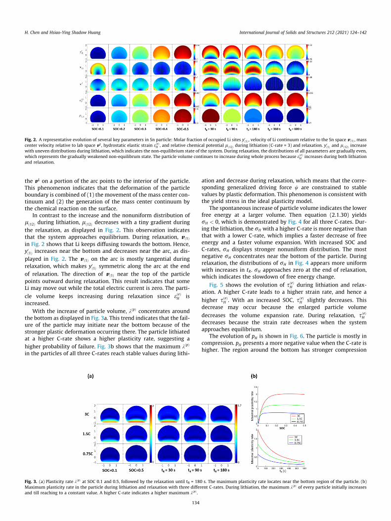
Fig. 2. A representative evolution of several key parameters in Sn particle: Molar fraction of occupied Li sites y0ð1Þ , velocity of Li continuum relative to the Sn space v ð1Þ , masscenter velocity relative to lab space vL , hydrostatic elastic strain eðeÞH , and relative chemical potential lð12Þ during lithiation (C-rate = 3) and relaxation. y0ð1Þ and lð12Þ increasewith uneven distributions during lithiation, which indicates the non-equilibrium state of the system. During relaxation, the distributions of all parameters are gradually even,which represents the gradually weakened non-equilibrum state. The particle volume continues to increase during whole process because eðeÞH increases during both lithiationand relaxation.


the vL on a portion of the arc points to the interior of the particle.This phenomenon indicates that the deformation of the particleboundary is combined of (1) the movement of the mass center con-tinuum and (2) the generation of the mass center continuum bythe chemical reaction on the surface.

In contrast to the increase and the nonuniform distribution oflð12Þ during lithiation, lð12Þ decreases with a tiny gradient duringthe relaxation, as displayed in Fig. 2. This observation indicatesthat the system approaches equilibrium. During relaxation, v ð1Þin Fig. 2 shows that Li keeps diffusing towards the bottom. Hence,y0ð1Þ increases near the bottom and decreases near the arc, as dis-played in Fig. 2. The v ð1Þ on the arc is mostly tangential duringrelaxation, which makes y0ð1Þ symmetric along the arc at the endof relaxation. The direction of v ð1Þ near the top of the particlepoints outward during relaxation. This result indicates that someLi may move out while the total electric current is zero. The parti-

cle volume keeps increasing during relaxation since eðeÞH isincreased.

With the increase of particle volume, kðpÞ concentrates aroundthe bottom as displayed in Fig. 3a. This trend indicates that the fail-ure of the particle may initiate near the bottom because of thestronger plastic deformation occurring there. The particle lithiatedat a higher C-rate shows a higher plasticity rate, suggesting ahigher probability of failure. Fig. 3b shows that the maximum kðpÞ

in the particles of all three C-rates reach stable values during lithi-

Fig. 3. (a) Plasticity rate kðpÞ at SOC 0.1 and 0.5, followed by the relaxation until tR = 180Maximum plasticity rate in the particle during lithiation and relaxation with three differand till reaching to a constant value. A higher C-rate indicates a higher maximum kðpÞ .

134

ation and decrease during relaxation, which means that the corre-sponding generalized driving force w are constrained to stablevalues by plastic deformation. This phenomenon is consistent withthe yield stress in the ideal plasticity model.

The spontaneous increase of particle volume indicates the lowerfree energy at a larger volume. Then equation (2.1.30) yieldsrH < 0, which is demonstrated by Fig. 4 for all three C-rates. Dur-ing the lithiation, the rH with a higher C-rate is more negative thanthat with a lower C-rate, which implies a faster decrease of freeenergy and a faster volume expansion. With increased SOC andC-rates, rH displays stronger nonuniform distribution. The mostnegative rH concentrates near the bottom of the particle. Duringrelaxation, the distributions of rH in Fig. 4 appears more uniformwith increases in tR. rH approaches zero at the end of relaxation,which indicates the slowdown of free energy change.

Fig. 5 shows the evolution of sðeÞH during lithiation and relax-ation. A higher C-rate leads to a higher strain rate, and hence a

higher sðeÞH . With an increased SOC, sðeÞH slightly decreases. Thisdecrease may occur because the enlarged particle volume

decreases the volume expansion rate. During relaxation, sðeÞH

decreases because the strain rate decreases when the systemapproaches equilibrium.

The evolution of pH is shown in Fig. 6. The particle is mostly incompression. pH presents a more negative value when the C-rate ishigher. The region around the bottom has stronger compression

s. The maximum plasticity rate locates near the bottom region of the particle. (b)ent C-rates. During lithiation, the maximum kðpÞ of every particle initially increases

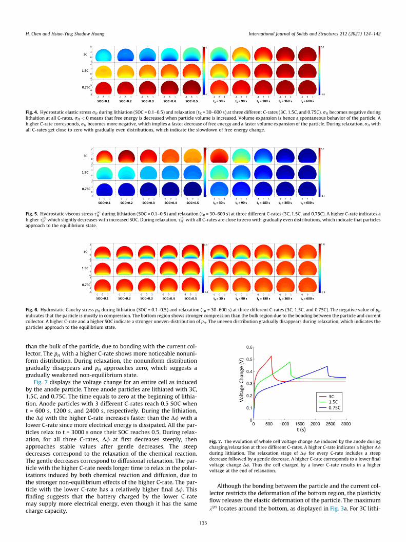
Fig. 4. Hydrostatic elastic stress rH during lithiation (SOC = 0.1–0.5) and relaxation (tR = 30–600 s) at three different C-rates (3C, 1.5C, and 0.75C). rH becomes negative duringlithaition at all C-rates. rH < 0 means that free energy is decreased when particle volume is increased. Volume expansion is hence a spontaneous behavior of the particle. Ahigher C-rate corresponds, rH becomes more negative, which implies a faster decrease of free energy and a faster volume expansion of the particle. During relaxation, rH withall C-rates get close to zero with gradually even distributions, which indicate the slowdown of free energy change.

Fig. 5. Hydrostatic viscous stress sðeÞH during lithiation (SOC = 0.1–0.5) and relaxation (tR = 30–600 s) at three different C-rates (3C, 1.5C, and 0.75C). A higher C-rate indicates ahigher sðeÞH which slightly decreases with increased SOC. During relaxation, sðeÞH with all C-rates are close to zero with gradually even distributions, which indicate that particlesapproach to the equilibrium state.

Fig. 6. Hydrostatic Cauchy stress pH during lithiation (SOC = 0.1–0.5) and relaxation (tR = 30–600 s) at three different C-rates (3C, 1.5C, and 0.75C). The negative value of pH

indicates that the particle is mostly in compression. The bottom region shows stronger compression than the bulk region due to the bonding between the particle and currentcollector. A higher C-rate and a higher SOC indicate a stronger uneven-distribution of pH . The uneven distribution gradually disappears during relaxation, which indicates theparticles approach to the equilibrium state.

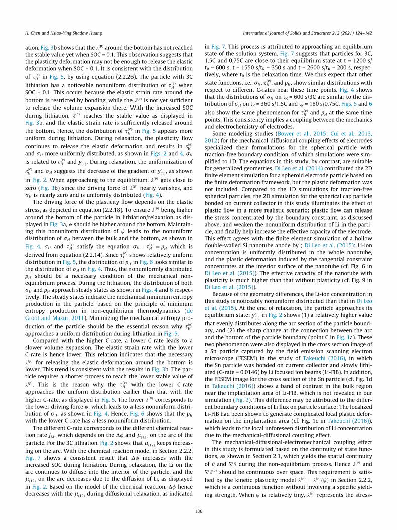
Fig. 7. The evolution of whole cell voltage change D/ induced by the anode duringcharging/relaxation at three different C-rates. A higher C-rate indicates a higher D/during lithiation. The relaxation stage of D/ for every C-rate includes a steepdecrease followed by a gentle decrease. A higher C-rate corresponds to a lower finalvoltage change D/. Thus the cell charged by a lower C-rate results in a highervoltage at the end of relaxation.


than the bulk of the particle, due to bonding with the current col-lector. The pH with a higher C-rate shows more noticeable nonuni-form distribution. During relaxation, the nonuniform distributiongradually disappears and pH approaches zero, which suggests agradually weakened non-equilibrium state.

Fig. 7 displays the voltage change for an entire cell as inducedby the anode particle. Three anode particles are lithiated with 3C,1.5C, and 0.75C. The time equals to zero at the beginning of lithia-tion. Anode particles with 3 different C-rates reach 0.5 SOC whent = 600 s, 1200 s, and 2400 s, respectively. During the lithiation,the D/ with the higher C-rate increases faster than the D/ with alower C-rate since more electrical energy is dissipated. All the par-ticles relax to t = 3000 s once their SOC reaches 0.5. During relax-ation, for all three C-rates, D/ at first decreases steeply, thenapproaches stable values after gentle decreases. The steepdecreases correspond to the relaxation of the chemical reaction.The gentle decreases correspond to diffusional relaxation. The par-ticle with the higher C-rate needs longer time to relax in the polar-izations induced by both chemical reaction and diffusion, due tothe stronger non-equilibrium effects of the higher C-rate. The par-ticle with the lower C-rate has a relatively higher final D/. Thisfinding suggests that the battery charged by the lower C-ratemay supply more electrical energy, even though it has the samecharge capacity.

135

Although the bonding between the particle and the current col-lector restricts the deformation of the bottom region, the plasticityflow releases the elastic deformation of the particle. The maximumkðpÞ locates around the bottom, as displayed in Fig. 3a. For 3C lithi-


ation, Fig. 3b shows that the kðpÞ around the bottom has not reachedthe stable value yet when SOC = 0.1. This observation suggests thatthe plasticity deformation may not be enough to release the elasticdeformation when SOC = 0.1. It is consistent with the distribution

of sðeÞH in Fig. 5, by using equation (2.2.26). The particle with 3C

lithiation has a noticeable nonuniform distribution of sðeÞH whenSOC = 0.1. This occurs because the elastic strain rate around thebottom is restricted by bonding, while the kðpÞ is not yet sufficientto release the volume expansion there. With the increased SOCduring lithiation, kðpÞ reaches the stable value as displayed inFig. 3b, and the elastic strain rate is sufficiently released around

the bottom. Hence, the distribution of sðeÞH in Fig. 5 appears moreuniform during lithiation. During relaxation, the plasticity flow

continues to release the elastic deformation and results in eðeÞH

and rH more uniformly distributed, as shown in Figs. 2 and 4. rH

is related to eðeÞH and y0ð1Þ. During relaxation, the uniformization of

eðeÞH and rH suggests the decrease of the gradient of y0ð1Þ, as shown

in Fig. 2. When approaching to the equilibrium, kðpÞ gets close tozero (Fig. 3b) since the driving force of kðpÞ nearly vanishes, andrH is nearly zero and is uniformly distributed (Fig. 4).

The driving force of the plasticity flow depends on the elasticstress, as depicted in equation (2.2.18). To ensure kðpÞ being higheraround the bottom of the particle in lithiation/relaxation as dis-played in Fig. 3a, w should be higher around the bottom. Maintain-ing this nonuniform distribution of w leads to the nonuniformdistribution of rH between the bulk and the bottom, as shown in

Fig. 4. rH and sðeÞH satisfy the equation rH þ sðeÞH ¼ pH which is

derived from equation (2.2.14). Since sðeÞH shows relatively uniformdistribution in Fig. 5, the distribution of pH in Fig. 6 looks similar tothe distribution of rH in Fig. 4. Thus, the nonuniformly distributedpH should be a necessary condition of the mechanical non-equilibrium process. During the lithiation, the distribution of bothrH and pH approach steady states as shown in Figs. 4 and 6 respec-tively. The steady states indicate the mechanical minimum entropyproduction in the particle, based on the principle of minimumentropy production in non-equilibrium thermodynamics (deGroot and Mazur, 2011). Minimizing the mechanical entropy pro-

duction of the particle should be the essential reason why sðeÞH

approaches a uniform distribution during lithiation in Fig. 5.Compared with the higher C-rate, a lower C-rate leads to a

slower volume expansion. The elastic strain rate with the lowerC-rate is hence lower. This relation indicates that the necessarykðpÞ for releasing the elastic deformation around the bottom islower. This trend is consistent with the results in Fig. 3b. The par-ticle requires a shorter process to reach the lower stable value of

kðpÞ. This is the reason why the sðeÞH with the lower C-rateapproaches the uniform distribution earlier than that with thehigher C-rate, as displayed in Fig. 5. The lower kðpÞ corresponds tothe lower driving force w, which leads to a less nonuniform distri-bution of rH , as shown in Fig. 4. Hence, Fig. 6 shows that the pH

with the lower C-rate has a less nonuniform distribution.The different C-rate corresponds to the different chemical reac-

tion rate JM , which depends on the D/ and lð12Þ on the arc of theparticle. For the 3C lithiation, Fig. 2 shows that lð12Þ keeps increas-ing on the arc. With the chemical reaction model in Section 2.2.2,Fig. 7 shows a consistent result that D/ increases with theincreased SOC during lithiation. During relaxation, the Li on thearc continues to diffuse into the interior of the particle, and thelð12Þ on the arc decreases due to the diffusion of Li, as displayedin Fig. 2. Based on the model of the chemical reaction, D/ hencedecreases with the lð12Þ during diffusional relaxation, as indicated

136

in Fig. 7. This process is attributed to approaching an equilibriumstate of the solution system. Fig. 7 suggests that particles for 3C,1.5C and 0.75C are close to their equilibrium state at t = 1200 s/tR = 600 s, t = 1550 s/tR = 350 s and t = 2600 s/tR = 200 s, respec-tively, where tR is the relaxation time. We thus expect that other

state functions, i.e., rH , sðeÞH , and pH , show similar distributions withrespect to different C-rates near these time points. Fig. 4 showsthat the distributions of rH on tR = 600 s/3C are similar to the dis-tribution of rH on tR = 360 s/1.5C and tR = 180 s/0.75C. Figs. 5 and 6

also show the same phenomenon for sðeÞH and pH at the same timepoints. This consistency implies a coupling between the mechanicsand electrochemistry of electrodes.

Some modeling studies (Bower et al., 2015; Cui et al., 2013,2012) for the mechanical-diffusional coupling effects of electrodesspecialized their formulations for the spherical particle withtraction-free boundary condition, of which simulations were sim-plified to 1D. The equations in this study, by contrast, are suitablefor generalized geometries. Di Leo et al. (2014) contributed the 2Dfinite element simulation for a spheroid electrode particle based onthe finite deformation framework, but the plastic deformation wasnot included. Compared to the 1D simulations for traction-freespherical particles, the 2D simulation for the spherical cap particlebonded on current collector in this study illuminates the effect ofplastic flow in a more realistic scenario: plastic flow can releasethe stress concentrated by the boundary constraint, as discussedabove, and weaken the nonuniform distribution of Li in the parti-cle, and finally help increase the effective capacity of the electrode.This effect agrees with the finite element simulation of a hollowdouble-walled Si nanotube anode by ; Di Leo et al. (2015): Li-ionconcentration is uniformly distributed in the whole nanotube,and the plastic deformation induced by the tangential constraintconcentrates at the interior surface of the nanotube (cf. Fig. 6 inDi Leo et al. (2015)). The effective capacity of the nanotube withplasticity is much higher than that without plasticity (cf. Fig. 9 inDi Leo et al. (2015)).

Because of the geometry differences, the Li-ion concentration inthis study is noticeably nonuniform distributed than that in Di Leoet al. (2015). At the end of relaxation, the particle approaches itsequilibrium state: y0ð1Þ in Fig. 2 shows (1) a relatively higher valuethat evenly distributes along the arc section of the particle bound-ary, and (2) the sharp change at the connection between the arcand the bottom of the particle boundary (point C in Fig. 1a). Thesetwo phenomenon were also displayed in the cross section image ofa Sn particle captured by the field emission scanning electronmicroscope (FESEM) in the study of Takeuchi (2016), in whichthe Sn particle was bonded on current collector and slowly lithi-ated (C-rate = 0.0146) by Li focused ion beams (Li-FIB). In addition,the FESEM image for the cross section of the Sn particle (cf. Fig. 1din Takeuchi (2016)) shows a band of contrast in the bulk regionnear the implantation area of Li-FIB, which is not revealed in oursimulation (Fig. 2). This difference may be attributed to the differ-ent boundary conditions of Li flux on particle surface: The localizedLi-FIB had been shown to generate complicated local plastic defor-mation on the implantation area (cf. Fig. 1c in Takeuchi (2016)),which leads to the local unforeseen distribution of Li concentrationdue to the mechanical-diffusional coupling effect.

The mechanical-diffusional-electromechanical coupling effectin this study is formulated based on the continuity of state func-tions, as shown in Section 2.1, which yields the spatial continuityof h and rh during the non-equilibrium process. Hence kðpÞ andrkðpÞ should be continuous over space. This requirement is satis-fied by the kinetic plasticity model kðPÞ ¼ kðPÞ wð Þ in Section 2.2.2,which is a continuous function without involving a specific yield-ing strength. When w is relatively tiny, kðPÞ represents the stress-


induced creep. The kinetic plasticity model shows the similarresponse of plastic strain to the ideal plasticity model (Hill, 1998)when Kw in equations (2.2.21) and (2.2.22) is large enough. Thesmooth transition between the elastic region and plastic regionof electrodes has been formulated using the piecewise power func-tions in Bower et al. (2011), Bower et al. (2015), Cui et al. (2012),Cui et al. (2013), and Di Leo et al. (2015). Compared to the piece-wise plasticity models, the kinetic plasticity model helps simplifythe procedure of solving the system equations by excluding theradial return algorithm (Simo and Taylor, 1986; Wang and Atluri,1994) used for locating the plastic region in the system.

The chemical potential model that includes the finite deforma-tion of electrodes has been studied by Cui et al. (2012), Cui et al.(2013), in which the mechanical part of the chemical potentialmodel has a coefficient term @F�

@c

� �F;C that represents the deforma-

tion change induced by the concentration change for the interme-diate state under the fixed total deformation and the fixedstiffness. However, @F�

@c

� �F;C relates to not only the material property

(i.e., the expansion ratio) but also the change of elastic state, whichis implicit and needs to be solved. In contrast, the relative chemicalpotential model in this study uses the material property KD only toexplicitly show the mechanical part. In some other studies of mod-eling the finite deformation of electrodes, e.g., Bower et al. (2011),Dal and Miehe (2015), Di Leo et al. (2014), Di Leo et al. (2015), andBucci et al. (2016), the chemical potential are modeled based onthe Larche-Cahnmodel (Larché and Cahn, 1973) shown in equation(1.1). However, the Larche-Cahn model (Larché and Cahn, 1973) isbased on the assumptions that (1) the deformation of the system issmall and thermodynamically reversible and (2) the molar mass ofLi-ion is much less than the molar mass of site component,Mð1Þ Mð2Þ. The assumption of small deformation would resultin the metric change negligible. Thermodynamic reversibilitywould result in the integral to be path independent. Mð1Þ Mð2Þindicates constant density and v ¼ 0, which linearize the rateequations (2.2.12), (2.2.45), and (2.2.46). Then directly integratingthe rate equations yields the Larche-Cahn model, which is a specialcase of the non-equilibrium model in this study. Using the Larche-Cahn model suggests the acceptance of above two assumptions.However, the assumption (1) is limited in the infinitesimal defor-mation and an equilibrium process. The assumption (2) oversim-plifies the diffusion of Li since the molar mass of Li should not benegligible for most electrode materials. Therefore, it is not plausi-ble to adopt the Larche-Cahn model to describe the chemicalpotential of electrodes with finite deformation or non-equilibrium process.

As Li atoms should share the stress of electrodes, we considerthe movement of lithium as a part of the deformation of the mix-tured system represented by the mass center contiuum. Thedeformation of the mixtured system should be formulated basedon the mass-conserved infinitesimal element instead of the mole-number-conserved infinitesimal element, because the differentmolar mass of components make the mass conservation con-flicted with the mole-number-conservation in the infinitesimalelement of mass center continuum. Thus, we use the mass frac-tions of components instead of the concentration of components,and the specific free energy instead of the free energy density toformulate the mixtured system. In the existing studies for model-ing the finite deformation of electrodes (Bower et al., 2011; Di Leoet al., 2014, 2015; Dal and Miehe, 2015; Bucci et al., 2016; Cuiet al., 2013, 2012), by contrast, the concentration of componentsand the free energy density are used in the formulations based onthe mole-number-conservation, suggesting that the movement ofLi atoms are not considered as a part of the deformation of themixture.

137

The mass-conserved infinitesimal element of the mixtured sys-tem is introduced by using multi metric spaces, in which everyspace reveals the deformation of every corresponding componentin the mixture. The method of multi metric spaces helps distributethe strains of the mixtured system conveniently: the Li-Sn systemincludes three metric spaces (i.e., mass center space, Sn space, andlab space), in which the Sn space is selected as the reference spacebecause (1) the elastic strain and the plastic strain rate of the mix-ture are assigned to the Sn continuum due to the interstitial mixingof the Li-Sn system, and (2) the Sn space is the Lagrangian space ofthe Sn continuum, which satisfies the requirement of the additivedecomposition of strain component (equation (2.1.11)) derivedfrom the metric-based definition of the finite strain (equation(2.1.10)). Compared to the multiplicative decomposition of defor-mation gradient used in the other modeling works for finite defor-mation of electrodes (Bower et al., 2011; Di Leo et al., 2014, 2015;Bucci et al., 2016; Cui et al., 2013, 2012), the additive decomposi-tion of strain component is linear, simpler and also valid for thefinite deformation of electrodes.

The method of multi metric spaces in this study reveals thediffusion-induced creep of electrodes. In the Li-Sn systemdescribed in the Sn space (i.e., reference space), the influences ofdiffusion-induced creep on the mixture (i.e., mass center contin-uum) are represented by the diffusion-induced convective effects,which are indicated by the terms including v (i.e., the mass centervelocity relative to the reference space) in rate equations (2.2.12),(2.2.45) and (2.2.46). In the relation between the electrical poten-tial and Li concentration of a Si film electrode measured by Pharret al. (2014), the electrical potential showed transient trend rever-sal with each change of C-rate during lithiation, and the rate of thetrend reversal is higher when the change of C-rate is larger (cf.Fig. 1 in Pharr et al. (2014)). This phenonmenon may be explainedby the influcence of diffusion-induced creep: At the moment ofinstantly increasing the C-rate of the Si film electrode during lithi-

ation, in the region of chemical reaction, eðeÞkj@vk

@zi and vk @eðeÞ

ij

@zk in equa-

tion (2.2.12) increase instantly, while the change of@eðeÞ

ij

@t may keepnegligible because of the viscosity of the electrode. Then increased_eðeÞij may decrease dlð12Þ=dt by equations (2.2.46) and (2.2.47) sinceKD < 0. Finally, the slope @/=@t is increased by equation (2.2.32). /hence transiently increases after each instant decrease induced byincreasing the C-rate, and vice versa. When the change of C-rate is

larger, the changes of terms eðeÞkj@vk

@zi and vk @eðeÞ

ij

@zk in equation (2.2.12)are larger, finally the trend reversal of / is faster. As / is influencedby v in equation (2.2.12), the diffusion-induced creep should takepart in the mechanical-diffusional-electrochemical coupling effectof electrodes.

As the influence of the diffusion-induced creep, the termsincluding v in rate equations (2.2.12), (2.2.45) and (2.2.46) makethe integrals for elastic strain, elastic stress, and relative chemicalpotential related to the history of diffusion. Furthermore, the elas-tic stress is influenced by the rate of deformation, because of theviscous stress sðeÞ in equations (2.2.14) and (2.2.23). Therefore,the states of a mixtured system relate to the history and the rateof the evolution of the system, which is an essential feature ofthe non-equilibrium process. Compared to the framework that isbased on the rate functions for modeling the non-equilibrium pro-cess of electrodes in this study, the formulations in existing contri-butions (Bower et al., 2011; Di Leo et al., 2014, 2015; Bucci et al.,2016; Cui et al., 2013, 2012) are based on the assumed explicitexpressions of the free energy density without considering the vis-cosity and diffusion-induced creep, which are only suitable for thesystems in quasi-equilibrium process.


4. Conclusion

In this paper, we have developed a general theory to describethe evolution of a solid solution system with finite deformation.The system is considered as a non-equilibrium process rather thana quasi-equilibrium process. This fully self-consistent theory ishence formulated based on rate functions. Mechanics, diffusion,phase separation, chemical reaction and electrical potential ofthe system are coupled with each other in the formulation. Thekey function of the coupling is the rate of the relative chemicalpotential that depends on the elastic strain rate and Li-ion fractionrate. The general theory has been applied to a simplified Li-Sn sys-tem in Li-ion batteries. We set multiple metric spaces to clarify theinfluence of the diffusion-induced creep of the system and to helpassign different strains conveniently. During the non-equilibriumprocess of the Li-Sn system, the entropy production rate of the sys-tem is composed of a mechanical component, a diffusional compo-nent, and a chemical reaction component. The mechanical part iscomprised of viscosity and plasticity and where the linearized vis-cosity is used. The plasticity and chemical reaction are formulatedbased on the transition-state theory. The kinetic formulation of theplasticity generates a continuous interface between elastic defor-mation and plastic deformation which helps obviate the steps ofidentifying the plastic region in the system and simplify the proce-dure of solving the plasticity of electrodes.

Three Sn electrode particles with initial spherical cap geome-tries and appropriate boundary conditions have been numericallysimulated using the finite difference method coded with MATLAB.We have compared the lithiated processes of the particles withthree different C-rates, including the lithiation and relaxation.The simulation results show that the bottom region of each particlehas more plastic deformation than the bulk region. The plasticdeformation helps release the volume expansion around the bot-tom region, although it is bonded. The particle with a higher C-rate needs a longer process to obtain higher rate of plastic defor-mation, which releases the faster volume expansion around thebottom. During lithiation, the electrical potential of the particlewith a higher C-rate shows more polarization. After relaxation,the particle with a lower C-rate consists more electric energy, eventhough the final electric capacities of all particles are the same.

With the rigorous mathematical formulation, we illuminate theevolution of a solid solution system in details. Our developed the-ory and simulation help better understand the mechanical-diffusional-electrochemical coupling effect in Li-ion batteries. Someinnovations in this study, such as multiple metric spaces for differ-ent components, diffusion-induced creep/convection, viscosity,and kinetic plasticity, may provide more insight into the descrip-tion of continuous mixtures especially at non-equilibrium.

Declaration of Competing Interest

The authors declare that they have no known competing finan-cial interests or personal relationships that could have appearedto influence the work reported in this paper.

Appendix A

A1. Introduction to the metric-based kinematics of finite deformation

The initial configuration and the deformed configuration of a con-tinuum correspond to two spaces with curvilinear coordinateframes f1; f2; f3

� �and g1;g2;g3

� �respectively. The differential of

radius vector is invariant in both spaces: dr ¼ @r@fi

dfi ¼ @r@gj dg

j. The

basis of initial space and deformed space are defined by ei ¼ @r@fi

138

and ej ¼ @r@gj respectively, where ^ denotes the deformed space.

With the function relation fi ¼ fi g1;g2;g3� �

, we have

dr ¼ dgjej ¼ dfiei ¼ @fi

@gj dgjei, which yields

ej ¼ @fi

@gjei ðA1:1Þ

The function relation gi ¼ gi f1; f2; f3� �

yields

dgi ¼ @gi

@fjdfj ðA1:2Þ

Equations (A1.1) and (A1.2) show the transformations betweentwo spaces for the basis and components of dr respectively. Quan-tities which transform like the basis of dr, by equation (A1.1), isnamed covariant. Quantities which transform like the componentsof dr, by equation (A1.2), is named contravariant. Please note thedifferent locations of the dummy indices in equation (A1.1) andequation (A1.2). The transformations for covariant quantities andcontravariant quantities are mutually inverse. The indices ofcovariant quantities are subscripts. The indices of contravariantquantities are superscripts. A pair of the same indices that one issubscript and the other is superscripts indicates the Einstein sum-mation convention.

The metric of a space is defined as the dot product between twobase vectors of the space. The metric of the initial space isgij ¼ ei � ej. The contravariant metric gij is the inverse of gij:

gij� � ¼ gij

� ��1. We use gij to introduce the contravariant basis of

the initial space: ej ¼ gijei. The deformed space also has the corre-

sponding metric gij and contravariant basis ei.Based on the invariance of tensors, a 1st order tensor A and a

2nd order tensor T respectively satisfy below equations:

A ¼ Aiei ¼ Aiei ¼ Aiei ¼ Aie

i ðA1:3Þ

T ¼ Tijeiej ¼ Tijeiej ¼ Tijeie

j ¼ Tijeiej ¼ T ije

iej ¼ Ti

jeiej ðA1:4Þ

where Tij and T

i

j are called mixed components of T . The contravari-ant components, covariant components, and mixed components of

T in different spaces are transformed by Tij ¼ Tkl @gi

@fk@gj

@fl,

T ij ¼ Tkl@fk

@gi@fl

@gj, and Ti

j ¼ Tkl@gi

@fk@fl

@gj respectively.

The metric of a space can be used to change the indices location

of the tensor components in the space. For example, Ai ¼ Ajgij, and

T ij ¼ Tklgkiglj ¼ T

l

iglj. It can be proved that gij and gij are respectivelythe covariant and contravariant components of a tensor g, namedthe fundamental metric tensor, whose mixed components are equalto the Kronecker delta: gi

k ¼ ei � ek ¼ gijgjk ¼ dik. The mixed compo-nents of g are usually used to change the indices of quantities. Forexample, the trace of T is calculated by

Tr Tð Þ ¼ Tijeiej� �

: gklekel

� � ¼ Tijgkl ei � ek� �

ej � el� � ¼ Tijgklg

ki g

lj

¼ Tijgij ¼ Tii ¼ T

^ i

i

We consider the configuration of a deformed continuum as adeformed space. The covariant component of strain for the spacedeformation is defined as half of the metric change of the spacefrom initial state to final state, as shown below,

eij ¼ 12

g�ij � g

�ij

� �ðA1:5Þ

where eij is the covariant component of strain, g�ij and g

�ij are the

metric of the final space and the initial space respectively. eij can


be used to introduce two strain tensors with the same covariant

components but different contravariant basis: e� ¼ eije

�ie�j

and

e� ¼ eije

�ie�j. The tensor e

�is equivalent to the Green strain tensor when

the initial space is undeformed, which is proved below: The finalmetric and the initial metric are gij and gij respectively, which indi-

cates eij ¼ 12 gij � gij

� �, where the ^ in eij emphasizes the basis of

deformed space for strain tensor. With Fij ¼ @fi

@gj, we have

eijeiej ¼ 1

2gije

iej � gijeiej

� �¼ 1

2gklF

ki F

lje

iej � gijeiej

� �ðA1:6Þ

eijeiej ¼ 1

2ek � elð ÞFk

i Flje

iej � gijeiej

h i¼ 1

2Fki e

iek� �

� Fljele

j� �

� gijeiej

h iðA1:7Þ

The deformation gradient is a two-point tensor, which includesthe basis of two different spaces. As the initial space is unde-

formed, gijeiej ¼ I. We hence have,

e ¼ 12

FT � F � I� �

ðA1:8Þ

where the right side is the definition of Green strain tensor.When we decompose a deformation to multiple sequential pro-

cesses, we have the multiplicative decomposition of deformationgradient and the additive decomposition of strain component.The additive decomposition of strain component (equation(2.1.11)) is proved as below: For simplicity, we consider twosequential processes for a deformation, (a) and (b). Based on equa-tion (A1.5), the covariant component of strain for the process (a) is

eðaÞij ¼ 12

g�ðaÞij � g

�ðaÞij

� �¼ 1

2g�ðaÞij � gij

� �ðA1:9Þ

and the covariant component of strain for the process (b) is

eðbÞij ¼ 12

g�ðbÞij � g

�ðbÞij

� �¼ 1

2gij � g

�ðbÞij

� �ðA1:10Þ

Because processes (a) and (b) are sequential, we have g�ðaÞij ¼ g

�ðbÞij ,

summing equations (A1.9) and (A1.10) yields the additive decom-position below,

eij ¼ eðaÞij þ eðbÞij ðA1:11ÞHence, as two different mathematical forms of decomposing the

finite deformation, the multiplicative decomposition of deforma-tion gradient and the additive decomposition of strain component(equation (2.1.11)) are mutually consistent. Please note that onlythe covariant components in Lagrangian measure satisfy the addi-tive decomposition of strain component.

In a curvilinear coordinate frame, the covariant derivative andLaplacian for scalars, and the covariant derivatives for the covari-ant/contravariant components of 1st and 2nd order tensors, arelisted below:

riu ¼ @u@fi

r2u ¼ @2u@fi@fj

gij � @u@fk

Ckijg

ij

riwj ¼ @wj

@fiþwkCj

ki

riwj ¼ @wj

@fi�wkC

kji

139

riHjk ¼ @Hjk

@fiþ HlkCj

li þ HjlCkli

riHjk ¼ @Hjk

@fi� HmkC

mij � HjmC

mik

where Ckij is called Christoffel symbols. In Euclidean space and Rie-

mannian Space, Christoffel symbols are calculated as below,

Cijk ¼

12gis @gjs

@fkþ @gks

@fj� @gjk

@fs

� �

For more information about the metric-based continuummechanics, see the reference Sedov (1997).

A2. Generalized mass conservation equation

A density function f of a continuum can be written as

f ¼ f Z1; Z2; Z3; t� �

or f ¼ f z1; z2; z3; t� �

. The rate of the volume inte-

gral of f depends on the local rate of f and the deformation of thedomain of integration as shown below (Sedov, 1997):

ddt

ZVfdt ¼

ZV

@f@t

� �Z

þr � fvLt

� �� dt ðA2:1Þ

where vLt is the velocity of the domain of integration of the contin-

uum relative to the lab space. The rate of f for fixed Lagrangiancoordinates of the continuum has two forms below:

dfdt

¼ @f@t

� �Z

þ vLt � rf ðA2:2Þ

dfdt

¼ @f@t

� �zþ vt � rf ðA2:3Þ

where vt is the velocity of the domain of integration of the contin-uum relative to the reference space. The relation between vL

t and vt

is

vLt ¼ vt þ v� ðA2:4Þ

Substituting equations (A2.2), (A2.3), and (A2.4) into equation(A2.1) yields

ddt

ZVfdt ¼

ZV

@f@t

� �z

þr � fvtð Þ þ fr � v��

dt ðA2:5Þ

Based on mass conservation for component k, chemical reac-tions determine the variation of total mass which is equal to thevariation of the volume integral of qðkÞ, as shown in equations(A2.6) and (A2.7):

dmðkÞdt

¼ZV

Xj

nðjÞðkÞJðjÞdt ðA2:6Þ

dmðkÞdt

¼ ddt

ZVqðkÞ z1; z2; z3; t� �

dt ðA2:7Þ

Setting f ¼ qðkÞ and vt ¼ v ðkÞ in equation (A2.5) and combiningequation (A2.6) yield equation (2.1.1).

A3. Entropy production rate

Combining equations (2.1.12), (2.1.14), (2.1.15) and the diver-gence theorem yields

dZVuqdV ¼

ZV

qdqþXk

qðkÞ drLkð Þ � drL� �

� FLkð Þ þ p : rdrL

" #dV

ðA3:1Þ


Because qdV ¼ dm, which is conserved mass differential, thevariational of the total internal energy for the mass center contin-uum relates to the functional derivatives with respect to indepen-dent variables by

dZVuqdV ¼

ZV

dUds

� �e;x

dsþXl

dU

deðlÞij

!s;eðl0–lÞ ;x

deðlÞij

24

þXK�1

k

dUdxðkÞ

� �s;e;xðk0–kÞ

dxðkÞ

35qdV ðA3:2Þ

Combining equations (A3.1) and (A3.2), setting ds ¼ ds,

deðlÞij ¼ deðlÞij , dxðkÞ ¼ dxðkÞ, dq ¼ dq, drLðkÞ ¼ vLðkÞdt, and drL ¼ vLdt (vari-

ational are arbitrary and can be set following the real process), andusing equation (2.1.4) yield

qTdsþXl

rðlÞijdeðlÞij þXK�1

k

qlðkKÞdxðkÞ

¼ qdqþXKk

JðkÞ � FLkð Þdt þ p : rvLdt ðA3:3Þ

We assume that p is a symmetric tensor. Using the kinematicrelations equations (A3.4) and (A3.5) for strain rate and strainsyields equation (A3.6):

_eij ¼ 12

rivLj þrjvL

i

� �ðA3:4Þ

eij ¼Xl

eðlÞij ðA3:5Þ

p : rvLdt ¼ p : _edt ¼ pijdeij ¼Xl

pijdeðlÞij ðA3:6Þ

Then, substitutingPK

k JðkÞ ¼ 0, the definition of heat fluxqdq ¼ �r � JQdt, equations (2.1.26), (2.1.27), and (A3.6) intoequation (A3.3) yields equations (A3.7), (A3.8), and (A3.9) forentropy change, entropy flow and entropy production rate,respectively. Using equations (A3.10) and (2.1.25) we haveequation (2.1.24).

qdsdt

¼ �r � JS þ h ðA3:7Þ

JS ¼1T

JQ �XK�1

k

lðkKÞJðkÞ

!ðA3:8Þ

Th ¼ �Js � rT þXl

pij � rðlÞij� �de^ ðlÞijdt

�XK�1

k

JðkÞ � rWLðkKÞ þ

Xj

JðjÞAðjÞC

ðA3:9Þ

_eðlÞij ¼ deðlÞij

dtðA3:10Þ

A4. Relative chemical potential

Because s is assumed to be independent of rxð1Þ and reðlÞ, wehave

@s@xð1Þ

� �T;:::

¼ f xð1Þ; eðlÞij

� �ðA4:1Þ

140

It yields

d T@s

@xð1Þ

� �T;:::

" #¼ @s

@xð1Þ

� �T;:::

dT þ T@2s@x2ð1Þ

!T;:::

dxð1Þ

þXl

T@2s

@xð1Þ@eðlÞij

!T;:::

deðlÞij ðA4:2Þ

Based on the symmetry of the 2nd order derivatives of aF , equa-tions (2.1.30) and (2.1.31) yield

Xl

T@2s

@xð1Þ@eðlÞij

!T;:::

deðlÞij ¼Xl

� @cðlÞij

@xð1Þ

!T;:::

TdeðlÞij ðA4::3Þ

Substituting equation (A4.3) into equation (A4.2), we have

@s@xð1Þ

� �T;:::

dT þ T@2s@x2ð1Þ

!T;:::

dxð1Þ

¼ d T@s

@xð1Þ

� �T;:::

" #þ T

@c@xð1Þ

� �T;:::

gijdeðeÞij ðA4:4Þ

Using equation (A4.4) in equation (2.1.33) yields

dlHOMð12Þ ¼ �d T@s

@xð1Þ

� �T;:::

" #� T

@c@xð1Þ

� �T;:::

gijdeðeÞij

þ jgijdeðeÞij þ @2u@x2ð1Þ

!T;:::

dxð1Þ ðA4:5Þ

The parameter tensors with the 1st and 3rd orders are zero inisotropic material (Sedov, 1997). Using equation (2.1.29) we sim-plify equation (2.1.34) to

dliINHð12Þ ¼ xrspi

rð12ÞdrpeðeÞrs þ Kð12Þg

iqdrqxð1Þ ðA4:6Þwith defining a material property

@2u

@rixð1Þ@rqxð1Þ¼ K

iq

rð12Þ ¼ Kð12Þgiq ðA4::7Þ

The specific entropy s is related to the molar entropy sM com-

posed of a fraction part sMF ¼ sMF y0ð1Þ� �

and a deformation part

sMD ¼ sMD eðlÞij� �

as shown below:

s ¼ Sm

¼ Nð2ÞNB

msM ¼ xð2Þ

NB

Mð2ÞsMF þ sMDð Þ ðA4:8Þ

The fraction part obeys the entropy of the ideal solution asshown below (DeHoff, 2006):

sMF ¼ �R y0ð1Þlny0ð1Þ þ 1� y0ð1Þ

� �ln 1� y0ð1Þ� �h i

ðA4:9Þ

Equation (A4.9) yields

@

@xð1Þxð2Þ

NB

Mð2ÞsMF

� �T;:::

¼ �R1

Mð1Þln

y0ð1Þy0ð2Þ

� NB

Mð2Þlny0ð2Þ

" #ðA4:10Þ

We define the excess relative chemical potential as below:

lEXð12Þ ¼ lHOMð12Þ þ T@

@xð1Þxð2Þ

NB

Mð2ÞsMF

� �T;:::

ðA4:11Þ

Substituting equations (A4.8) and (A4.11) into equation (A4.5)yields

dlEXð12Þ ¼NB

Mð2ÞTdsMD � T

@c@xð1Þ

� �T;:::

gijdeðeÞij þ jgijdeðeÞij

þ @2u@x2ð1Þ

!T;:::

dxð1Þ ðA4:12Þ


where c is related to the stiffness and thermal expansion ratio asshown below

c^ ðeÞij ¼ cg

^ ij ¼ � @

@e^ðeÞkl

r^ ij

HOM

q

0@

1A

xð1Þ ;e^ðeÞmn–kl

@e^ ðeÞkl

@T

0@

1A

rHOMq

¼ � kqg^ ij

g^ kl þ Gqg

^ ik

g^ jl þ Gqg

^ il

g^ jk

� �aTg

^

kl ðA4:13Þ

Thus the coupling coefficient in the relative chemical potentialof a isotropic material is

KD ¼ j� T@c@xð1Þ

� �T;:::

� Txð2Þ

c ðA4:14Þ

With defining a material property h ¼ @2u@x2ð1Þ

� �T;:::

, substituting

equation (A4.14) into equation (A4.12) yields equation (2.2.46).

We assume liINHð12Þ is a 1st order homogeneous function of

rpeðeÞrs and rqxð1Þ. Equation (A4.6) yields

liINHð12Þ ¼ xrspi

r rpeðeÞrs þ Kð12Þg

iqrqxð1Þ ðA4:15Þwhere xrspi

r for isotropic material satisfies

xrspir ¼ xI g

rsgpi þxIIAgrpgsi þxIIBg

rigsp ðA4:16ÞFor simplicity, we assume xIIA ¼ xIIB ¼ 0. Combining equations

(2.1.21), (A4.10), (A4.11), (A4.15) and (A4.16) yields equation

(2.2.47). If @c@xð1Þ

� �T;:::

¼ 0, we have equation (2.2.48). Equation

(2.2.49) is obtained from equation (A4.13).

A5. Transformed equations

We divide the relative chemical potential into a homogeneous-logarithm part and an inhomogeneous-excess part, lð12Þ ¼lHLð12Þ þ lIEð12Þ with

lHLð12Þ ¼ RT1

Mð1Þln

y0ð1Þy0ð2Þ

� NB

Mð2Þlny0ð2Þ

" #ðA5:1Þ

Using equations (2.2.47) and (A5.1) yields equation (2.3.15).Combining equations (2.2.1), (2.2.2), (2.2.3), (2.2.28), (2.2.47),(2.3.2), (2.3.3), and (2.3.15) yields equations (2.3.1) and (2.3.6).Combining equations (2.1.12), (2.1.13), and vL ¼ v þ vL

ð2Þ yieldsequation (2.3.4). Using equations (2.2.14) and (2.2.26) we haveequation (2.3.5).

A6. Relation between D and L

Using equations (2.1.5) and (2.2.1), the flux of Li can be writtenas

Jð1Þ ¼ qð1Þxð2Þv ð1Þ ¼ cð1ÞMð1Þxð2Þv ð1Þ ðA6:1Þwhere cð1Þ is the concentration of Li. To estimate the relation

between D and L, we only consider lHLð12Þ in the diffusion for sim-plicity, as shown below,

Jð1Þ � LTrlHLð12Þ ¼ �LR

1Mð1Þy0ð1Þy

0ð2Þ

þ NB

Mð2Þy0ð2Þ

!ry0ð1Þ ðA6:2Þ

The Fick’s 1st law yields

cð1Þv ð1Þ ¼ �Drcð1Þ ¼ �DcMAXry0ð1Þ ¼ �DNBqð2ÞMð2Þ

ry0ð1Þ ðA6:3Þ

Combining equations (A6.1), (A6.2), (A6.3), and (2.2.29) yieldsthe expression of D as shown below,

141

D ¼RL0f L Mð2Þ þMð1ÞNBy0ð1Þ

� �2NBqð2ÞM

2ð1ÞMð2Þy0ð1Þy

0ð2Þ

ðA6:4Þ

A7. Differential of expanded surface area

Initially, the area differential of the particle surface is governedby

dl0j j2 ¼ g�ð2Þijdzidzj ¼ dz1

� �2 þ dz3� �2 ðA7:1Þ

and

d10j j2 ¼ g�ð2Þ22 dz2� �2 ¼ z1

� �2dz2� �2 ðA7:2Þ

where dl0 is the initial length of the infinitesimal arc perpendicularto the initial basis vector e2 on the particle surface and d10 is the ini-tial length of the infinitesimal arc parallel to the initial basis vectore2 on the particle surface. After the particle is deformed, the lengthsof the infinitesimal arcs have

dlj j2 ¼ gð2Þijdzidzj

¼ gð2Þ11 dz1� �2 þ 2gð2Þ13dz

1dz3 þ gð2Þ33 dz3� �2 ðA7:3Þ

and

d1j j2 ¼ gð2Þ22 dz2� �2 ¼ Z1

� �2dz2� �2 ðA7:4Þ

where dl is the length of the infinitesimal arc perpendicular tothe basis vector e2 on the particle surface and d1 is the length ofthe infinitesimal arc parallel to the basis vector e2 on the particlesurface. Hence, the initial and present area differentials respec-tively have

dA0ð Þ2 ¼ dl0j j2 d10j j2 ðA7:5Þand

dAð Þ2 ¼ dlj j2 d1j j2 ðA7:6ÞCombining equations (A7.1), (A7.2), (A7.3), (A7.4), (A7.5), and

(A7.6) yields equation (2.3.23).

A8. The component of vLð2Þ in the lab space

The relation between the components of a tensor in differentcoordinate frames yields equations (2.3.33) and (A8.1) (Sedov,1997);

gð2Þij ¼ gLpq@Zp

@zi@Zq

@zjðA8:1Þ

where gLpq is the metric of lab space. Using equation (A8.1) we have

equation (2.3.30). If we assume @Z3

@z1 < 0 and @Z3

@z3 > 0, equation (A8.1)implies equations (2.3.31) and (2.3.32).

References

Vetter, J., Novák, P., Wagner, M.R., Veit, C., Möller, K.-C., Besenhard, J.O., Winter, M.,Wohlfahrt-Mehrens, M., Vogler, C., Hammouche, A., 2005. Ageing mechanismsin lithium-ion batteries. J. Power Sources 147 (1-2), 269–281. https://doi.org/10.1016/j.jpowsour.2005.01.006.

Wang, D., Wu, X., Wang, Z., Chen, L., 2005. Cracking causing cyclic instability ofLiFePO4 cathode material. J. Power Sources 140 (1), 125–128. https://doi.org/10.1016/j.jpowsour.2004.06.059.

Piper, D.M., Yersak, T.A., Lee, S.-H., 2013. Effect of compressive stress onelectrochemical performance of silicon anodes. J. Electrochem. Soc. 160 (1),A77–A81. https://doi.org/10.1149/2.064301jes.

Shi, F., Song, Z., Ross, P.N., Somorjai, G.A., Ritchie, R.O., Komvopoulos, K., 2016.Failure mechanisms of single-crystal silicon electrodes in lithium-ion batteries.Nat. Commun. 7 (May), 1–8. https://doi.org/10.1038/ncomms11886.

https://doi.org/10.1016/j.jpowsour.2005.01.006




https://doi.org/10.1149/2.064301jes

https://doi.org/10.1038/ncomms11886


Cheng, Y.-T., Verbrugge, M.W., 2009. Evolution of stress within a spherical insertionelectrode particle under potentiostatic and galvanostatic operation. J. PowerSources 190 (2), 453–460. https://doi.org/10.1016/j.jpowsour.2009.01.021.

Kim, S., Huang, H.-Y., 2016. Mechanical stresses at the cathode–electrolyte interfacein lithium-ion batteries. J. Mater. Res. 31 (22), 3506–3512. https://doi.org/10.1557/jmr.2016.373.

Kim, S., Wee, J., Peters, K., Huang, H.-Y., 2018. Multiphysics coupling in lithium-ionbatteries with reconstructed porous microstructures. J. Phys. Chem. C 122 (10),5280–5290. https://doi.org/10.1021/acs.jpcc.7b12388.

Kim, S., Chen, H., Huang, H.Y.S., 2019. Coupled mechanical and electrochemicalanalyses of three-dimensional reconstructed LiFePO4 by focused ion beam/scanning electron microscopy in lithium-ion batteries. J. Electrochem. EnergyConvers. Storage 16 (1), 1–7. https://doi.org/10.1115/1.4040760.

Christensen, J., Newman, J., 2006. Stress generation and fracture in lithium insertionmaterials. J. Solid State Electrochem. 10 (5), 293–319. https://doi.org/10.1007/s10008-006-0095-1.

Bower, A.F., Guduru, P.R., Sethuraman, V.A., 2011. A finite strain model of stress,diffusion, plastic flow, and electrochemical reactions in a lithium-ion half-cell. J.Mech. Phys. Solids 59 (4), 804–828. https://doi.org/10.1016/j.jmps.2011.01.003.

Di Leo, C.V., Rejovitzky, E., Anand, L., 2014. A Cahn-Hilliard-type phase-field theoryfor species diffusion coupled with large elastic deformations: application tophase-separating Li-ion electrode materials. J. Mech. Phys. Solids 70 (1), 1–29.https://doi.org/10.1016/j.jmps.2014.05.001.

Bucci, G., Swamy, T., Bishop, S., Sheldon, B.W., Chiang, Y.-M., Carter, W.C., 2017. Theeffect of stress on battery-electrode capacity. J. Electrochem. Soc. 164 (4), A645–A654. https://doi.org/10.1149/2.0371704jes.

Larché, F., Cahn, J.W., 1973. A linear theory of thermochemical equilibrium of solidsunder stress. Acta Metall. 26 (1), 53–60. https://doi.org/10.1016/0001-6160(78)90201-8.

Huggins, R.A., 2008. Negative electrodes in lithium cells. Adv. Batter. 123–149. doi:10.1007/978-0-387-76424-5_7.

Qi, Y., Hector Jr., L.G., James, C., Kim, K.J., 2014. Lithium concentration dependentelastic properties of battery electrode materials from first principlescalculations. J. Electrochem. Soc. 161 (11), F3010–F3018. https://doi.org/10.1149/2.0031411jes.

Wen, J., Wei, Y., Cheng, Y.-T., 2018. Stress evolution in elastic-plastic electrodesduring electrochemical processes: a numerical method and its applications. J.Mech. Phys. Solids 116, 403–415. https://doi.org/10.1016/j.jmps.2018.04.006.

Bower, A.F., Chason, E., Guduru, P.R., Sheldon, B.W., 2015. A continuum model ofdeformation, transport and irreversible changes in atomic structure inamorphous lithium–silicon electrodes. Acta Mater. 98, 229–241. https://doi.org/10.1016/j.actamat.2015.07.036.

Di Leo, C.V., Rejovitzky, E., Anand, L., 2015. Diffusion–deformation theory foramorphous silicon anodes: the role of plastic deformation on electrochemicalperformance. Int. J. Solids Struct. 67-68, 283–296. https://doi.org/10.1016/j.ijsolstr.2015.04.028.

Bower, A.F., Guduru, P.R., Chason, E., 2015. Analytical solutions for composition andstress in spherical elastic–plastic lithium-ion electrode particles containing apropagating phase boundary. Int. J. Solids Struct. 69-70, 328–342. https://doi.org/10.1016/j.ijsolstr.2015.05.018.

Dal, H., Miehe, C., 2015. Computational electro-chemo-mechanics of lithium-ionbattery electrodes at finite strains. Comput. Mech. 55 (2), 303–325. https://doi.org/10.1007/s00466-014-1102-5.

Bucci, G., Chiang, Y.-M., Carter, W.C., 2016. Formulation of the coupledelectrochemical–mechanical boundary-value problem, with applications totransport of multiple charged species. Acta Mater. 104, 33–51. https://doi.org/10.1016/j.actamat.2015.11.030.

Kang, B., Ceder, G., 2009. Battery materials for ultrafast charging and discharging.Nature 458 (7235), 190–193. https://doi.org/10.1038/nature07853.

Xie, J., Oudenhoven, J.F.M., Harks, P.-P., Li, D., Notten, P.H.L., 2015. Chemical vapordeposition of lithium phosphate thin-films for 3D all-solid-state li-ion batteries.J. Electrochem. Soc. 162 (3), A249–A254. https://doi.org/10.1149/2.0091503jes.

Thompson, A.P., Plimpton, S.J., Mattson, W., 2009. General formulation of pressureand stress tensor for arbitrary many-body interaction potentials under periodicboundary conditions. J. Chem. Phys. 131 (15), 154107. https://doi.org/10.1063/1.3245303.

142

Jones, R.B., 1965. Diffusion creep in polycrystalline magnesium. Nature 207 (70),1965.

Pharr, M., Suo, Z., Vlassak, J.J., 2014. Variation of stress with charging rate due tostrain-rate sensitivity of silicon electrodes of Li-ion batteries. J. Power Sources270, 569–575. https://doi.org/10.1016/j.jpowsour.2014.07.153.

Whittingham, M.S., 2004. Lithium batteries and cathode materials. Chem. Rev. 104(10), 4271–4302. https://doi.org/10.1021/cr020731c.

Song, Y.C., Li, Z.Z., Soh, A.K., Zhang, J.Q., 2015. Diffusion of lithium ions anddiffusion-induced stresses in a phase separating electrode under galvanostaticand potentiostatic operations: phase field simulations. Mech. Mater. 91, 363–371. https://doi.org/10.1016/j.mechmat.2015.04.015.

ChiuHuang, C.-K., Shadow Huang, H.-Y., 2013. Stress evolution on the phaseboundary in LiFePO 4 Particles. J. Electrochem. Soc. 160 (11), A2184–A2188.https://doi.org/10.1149/2.079311jes.

Cui, Z., Gao, F., Qu, J., 2013. Interface-reaction controlled diffusion in binary solidswith applications to lithiation of silicon in lithium-ion batteries. J. Mech. Phys.Solids 61 (2), 293–310. https://doi.org/10.1016/j.jmps.2012.11.001.

Sedov, L.I., 1997. Mechanics of Continuous Media. World Scientific.Sedov, L.I., 1965. Introduction to the Mechanics of a Continuous Medium. Addison-

Wesley.de Groot, S.R., Mazur, P., 2011. Non-equilibrium Thermodynamics. Dover

Publications.Gelfand, I.M., Fomin, S.V., 2000. The Calculus of Variations. Dover Publications.Kearsley, E.A., Fong, J.T., 1975. Linearly independent sets of isotropic Cartesian

tensors of ranks up to eight. J. Res. Natl. Bur. Stand. Sect. B Math. Sci. 79B (1), 49.https://doi.org/10.6028/jres.079b.005.

DeHoff, R., 2006. Thermodynamics in Materials Science. CRC Press, p. 624.Persson, P.O., Strang, G., 2004. A simple mesh generator in MATLAB. SIAM Rev. 46

(2), 329–345. https://doi.org/10.1137/S0036144503429121.Perrone, N., Kao, R., 1975. A general finite difference method for arbitrary meshes.

Comput. Struct. 5 (1), 45–57. https://doi.org/10.1016/0045-7949(75)90018-8.Takeuchi, S. et al., 2016. Editors’ choice communication—comparison of nanoscale

focused ion beam and electrochemical lithiation in b-Sn microspheres. J.Electrochem. Soc. 163 (6), A1010–A1012. https://doi.org/10.1149/2.1161606jes.

Zheng, Q., Mauro, J.C., 2017. Viscosity of glass-forming systems. J. Am. Ceram. Soc.100 (1), 6–25. https://doi.org/10.1111/jace.14678.

Maxisch, T., Ceder, G., 2006. Elastic properties of olivine Lix FePO4 from firstprinciples. Phys. Rev. B Condens. Matter Mater. Phys. 73 (17), 1–4. https://doi.org/10.1103/PhysRevB.73.174112.

Stournara, M.E., Guduru, P.R., Shenoy, V.B., 2012. Elastic behavior of crystalline Li-Snphases with increasing Li concentration. J. Power Sources 208, 165–169. https://doi.org/10.1016/j.jpowsour.2012.02.022.

Shenoy, V.B., Johari, P., Qi, Y., 2010. Elastic softening of amorphous and crystallineLi-Si Phases with increasing Li concentration: a first-principles study. J. PowerSources 195 (19), 6825–6830. https://doi.org/10.1016/j.jpowsour.2010.04.044.

Ding, N. et al., 2009. Determination of the diffusion coefficient of lithium ions innano-Si. Solid State Ionics 180 (2–3), 222–225. https://doi.org/10.1016/j.ssi.2008.12.015.

Shi, J., Wang, Z., Fu, Y.Q., 2016. Density functional theory study of diffusion oflithium in Li–Sn alloys. J. Mater. Sci. 51 (6), 3271–3276. https://doi.org/10.1007/s10853-015-9639-z.

Marcicki, J., Conlisk, A.T., Rizzoni, G., 2014. A lithium-ion battery model includingelectrical double layer effects. J. Power Sources 251, 157–169. https://doi.org/10.1016/j.jpowsour.2013.11.001.

Cui, Z., Gao, F., Qu, J., 2012. A finite deformation stress-dependent chemicalpotential and its applications to lithium ion batteries. J. Mech. Phys. Solids 60(7), 1280–1295. https://doi.org/10.1016/j.jmps.2012.03.008.

Hill, R., 1998. The Mathematical Theory Of Plasticity. Oxford University Press, USA.Simo, J.C., Taylor, R.L., 1986. A return mapping algorithm for plane stress

elastoplasticity. Int. J. Numer. Methods Eng. 22 (3), 649–670. https://doi.org/10.1002/nme.1620220310.

Wang, L.H., Atluri, S.N., 1994. An analysis of an explicit algorithm and the radialreturn algorithm, and a proposed modification, in finite plasticity. Comput.Mech. 13 (5), 380–389. https://doi.org/10.1007/BF00512590.

Lide, D.R., 2005. CRC Handbook of Chemistry and Physics, Internet Version 2005,CRC Press. Taylor Fr. Boca Rat. FL, p. 2660. doi: 10.1016/0165-9936(91)85111-4.


https://doi.org/10.1557/jmr.2016.373

https://doi.org/10.1557/jmr.2016.373

https://doi.org/10.1021/acs.jpcc.7b12388

https://doi.org/10.1115/1.4040760

https://doi.org/10.1007/s10008-006-0095-1

https://doi.org/10.1007/s10008-006-0095-1

https://doi.org/10.1016/j.jmps.2011.01.003


https://doi.org/10.1149/2.0371704jes

https://doi.org/10.1016/0001-6160(78)90201-8

https://doi.org/10.1016/0001-6160(78)90201-8

https://doi.org/10.1149/2.0031411jes

https://doi.org/10.1149/2.0031411jes


https://doi.org/10.1016/j.actamat.2015.07.036






https://doi.org/10.1007/s00466-014-1102-5

https://doi.org/10.1007/s00466-014-1102-5



https://doi.org/10.1038/nature07853

https://doi.org/10.1149/2.0091503jes

https://doi.org/10.1063/1.3245303

https://doi.org/10.1063/1.3245303


https://doi.org/10.1021/cr020731c

https://doi.org/10.1016/j.mechmat.2015.04.015

https://doi.org/10.1149/2.079311jes


http://refhub.elsevier.com/S0020-7683(20)30443-1/h0155






https://doi.org/10.6028/jres.079b.005

https://doi.org/10.1137/S0036144503429121

https://doi.org/10.1016/0045-7949(75)90018-8

https://doi.org/10.1149/2.1161606jes

https://doi.org/10.1111/jace.14678

https://doi.org/10.1103/PhysRevB.73.174112

https://doi.org/10.1103/PhysRevB.73.174112




https://doi.org/10.1016/j.ssi.2008.12.015

https://doi.org/10.1016/j.ssi.2008.12.015

https://doi.org/10.1007/s10853-015-9639-z

https://doi.org/10.1007/s10853-015-9639-z





https://doi.org/10.1002/nme.1620220310

https://doi.org/10.1002/nme.1620220310

https://doi.org/10.1007/BF00512590

Modeling and simulation of the non-equilibrium process for ...

Documents

Transcript of Modeling and simulation of the non-equilibrium process for ...