Modeling and Simulation of Mineral Processing Systems
415
-
Upload
sanaamikhail -
Category
Documents
-
view
2.613 -
download
15
Transcript of Modeling and Simulation of Mineral Processing Systems


Modeling and Simulation ofMineral Processing Systems

This book is dedicated to mywife Helen

Modeling and Simulation ofMineral Processing SystemsR.P. King
Department of Metallurgical EngineeringUniversity of Utah, USA
Boston Oxford Auckland Johannesburg Melbourne New Delhi
Butterworth-HeinemannLinacre House, Jordan Hill, Oxford OX2 8DP225 Wildwood Avenue, Woburn, MA 01801-2041A division of Reed Educational and Professional Publishing Ltd
A member of the Reed Elsevier plc group
First published 2001
© R.P. King 2001
All rights reserved. No part of this publication may be reproducedin any material form (including photocopying or storing in anymedium by electronic means and whether or not transiently orincidentally to some other use of this publication) without thewritten permission of the copyright holder except in accordancewith the provisions of the Copyright, Designs and Patents Act 1988or under the terms of a licence issued by the Copyright LicensingAgency Ltd, 90 Tottenham Court Road, London, England W1P 9HE.Applications for the copyright holder’s written permission to reproduceany part of this publication should be addressed to the publishers
British Library Cataloguing in Publication DataKing, R.P.
Modeling and simulation of mineral processing systems1. Ore-dressing – Mathematical models 2. Ore-dressing – Computer simulationI. Title622.7
Library of Congress Cataloging in Publication DataKing, R.P. (Ronald Peter), 1938–
Modeling and simulation of mineral processing systems/R.P. King.p. cm.Includes bibliographical references and indexISBN 0 7506 4884 81. Ore-dressing–Mathematical models. 2. Ore-dressing–Computer simulation.I. Title.TN500.K498 2001622’.7’015118–dc21 2001037423
ISBN 0 7506 4884 8
For information on all Butterworth-Heinemannpublications visit our website at www.bh.com
Typeset at Replika Press Pvt Ltd, Delhi 110 040, IndiaPrinted and bound in Great Britain.
Preface
Quantitative modeling techniques and methods are central to the study anddevelopment of process engineering, and mineral processing is no exception.Models in mineral processing have been difficult to develop because of thecomplexity of the unit operations that are used in virtually all mineral recoverysystems. Chief among these difficulties is the fact that the feed material isinvariably a particulate solid. Many of the conventional mathematical modelingtechniques that are commonly used for process equipment have limitedapplication to particulate systems and models for most unit operations inmineral processing have unique features. Common ground is quite difficultto find. The one obvious exception is the population balance technique andthis forms a central thread that runs throughout the modeling techniquesthat are described in this book. The models that are described are certainlyincomplete in many respects, and these will be developed and refined bymany researchers during the years ahead. Nevertheless, the models are usefulfor practical quantitative work and many have been widely used to assist inthe design of new equipment and processes. Some of the newer models havenot yet been seriously tested in the industrial environment.
The book is written at a reasonably elementary level and should be accessibleto senior undergraduate and graduate students. A number of examples areincluded to describe the application of some of the less commonly usedmodels, and almost all of the models described in the book are included inthe MODSIM simulator that is available on the companion compact disk. Thereader is encouraged to make use of the simulator to investigate the behaviorof the unit operations by simulation.
The main advantage of using quantitative models is that they permit thecomplex interactions between different unit operations in a circuit to be exploredand evaluated. Almost all of the models described are strongly nonlinear andare not usually amenable to straightforward mathematical solutions, nor arethey always very convenient for easy computation using calculators or spreadsheets. In order to investigate interactions between models, the simulationmethod is strongly recommended, and the focus throughout this book hasbeen on the development of models that can be used in combination to simulatethe behavior of complex mineral dressing flowsheets. Simulation techniquesare popular because they allow complex problems to be tackled without theexpenditure of large resources. All the models described here can be usedwithin the MODSIM simulator so they are readily accessible to the reader.The models are transparent to the user and the models can be tried in isolationor in combination with other unit operations. MODSIM has proved itself tobe an excellent teaching tool both for conventional courses and, in recentyears, to support an Internet course delivered from the University of Utah. Ihope that distributing MODSIM widely, together with this book, will encourage
researchers and engineers to make use of this technique, which brings toevery engineer the results of many man-years of research endeavor that havecontributed to the development of the models. Simulation does have itslimitations and the reader is reminded that a simulator can not be reliedupon to provide an exact replica of any specific real plant operation. Thereliability of the simulator output is limited by the accumulated reliability ofthe component models.
The work of many researchers in the field has been inspiration for themodels that are described in this book. I have tried to extract from the researchliterature those modeling techniques that have proved to be useful andapplicable to practical situations and I have tried to identify those modelingmethods and process features that have been confirmed, at least partially, bycareful experimental observation. In this I am indebted to many students andcolleagues whose work has provided data, ideas and methods.
The preparation of a book is always a time-consuming task and I wish tothank my wife, Ellen, for her patience and encouragement while it was beingwritten and for typing much of the final version of the manuscript. Themanuscript went through many revisions and the early versions were typedby Karen Haynes. Kay Argyle typed the illustrative examples. It is a pleasureto acknowledge their contributions for which I am very grateful.
R.P. KingSalt Lake City
vi Preface
Contents
Preface v
1. Introduction 1
Bibliography 4References 4
2. Particle populations and distribution functions 5
2.1 Introduction 52.2 Distribution functions 62.3 The distribution density function 132.4 The distribution by number, the representative size and
population averages 132.5 Distributions based on particle composition 162.6 Joint distribution functions 172.7 Conditional distribution functions 192.8 Independence 312.9 Distributions by number 322.10 Internal and external particle coordinates and
distribution densities 342.11 Particle properties derived from internal coordinates 352.12 The population balance modeling method 352.13 The fundamental population balance equation 362.14 The general population balance equation for
comminution machines 40Bibliography 42References 43
3. Mineral liberation 45
3.1 The beta distribution for mineral liberation 463.2 Graphical representation of the liberation distribution 493.3 Quantitative prediction of mineral liberation 513.4 Simulating mineral liberation during comminution 583.5 Non-random fracture 693.6 Discretized Andrews-Mika diagram 723.7 Symbols used in this chapter 79Bibliography 79References 80

4. Size classification 81
4.1 Classification based on sieving–vibrating screens 814.2 The classification function 864.3 A simple kinetic model for screening 914.4 Classification based on differential settling – the
hydrocyclone 984.5 Terminal settling velocity 1024.6 Capacity limitations of the hydrocyclone 1244.7 Symbols used in this chapter 124References 125
5. Comminution operations 1275.1 Fracture of brittle materials 1275.2 Patterns of fracture when a single particle breaks 1295.3 Breakage probability and particle fracture energy 1325.4 Progeny size distribution when a single particle
breaks – the breakage function 1365.5 Energy requirements for comminution 1505.6 Crushing machines 1525.7 Grinding 1605.8 The continuous mill 1745.9 Mixing characteristics of operating mills 1795.10 Models for rod mills 1805.11 The population balance model for autogenous mills 1815.12 Models for the specific rate of breakage in ball mills 1875.13 Models for the specific rate of breakage in autogenous
and semi-autogenous mills 1975.14 Models for the breakage function in autogenous and
semi-autogenous mills 2015.15 Mill power and mill selection 2025.16 The batch mill 205Bibliography 209References 210
6. Solid–liquid separation 213
6.1 Thickening 2136.2 Useful models for the sedimentation velocity 2196.3 Simulation of continuous thickener operation 2206.4 Mechanical dewatering of slurries 2236.5 Filtration 227Bibliography 230References 231
7. Gravity separation 233
7.1 Manufactured-medium gravity separation 233
viii Contents

7.2 Quantitative models for dense-media separators 2347.3 Autogenous media separators 2437.4 Generalized partition function models for gravity
separation units 263Bibliography 266References 266
8. Magnetic separation 269
8.1 Behavior of particles in magnetic fields 2698.2 Forces experienced by a particle in a magnetic field 2728.3 Magnetic properties of minerals 2778.4 Magnetic separating machines 2788.5 Dry magnetic separation 2838.6 Wet high intensity magnetic separation 287Bibliography 288References 288
9. Flotation 289
9.1 A kinetic approach to flotation modeling 2909.2 A kinetic model for flotation 2939.3 Distributed rate constant kinetic model for flotation 3079.4 Bubble loading during flotation 3099.5 Rise times of loaded bubbles 3129.6 Particle detachment 3219.7 The froth phase 3239.8 Simplified kinetic models for flotation 3379.9 Symbols used in this chapter 346Bibliography 347References 348
10. Simulation of ore dressing plants 351
10.1 The nature of simulation 35110.2 Use of the simulator 35410.3 The flowsheet structure 35510.4 Simulation of single unit operations and simple
flowsheets 36310.5 Integrated flowsheets 37110.6 Symbols used in this chapter 393References 393
Appendix: Composition and specific gravities of somecommon minerals 395
Index 399
Contents ix

This Page Intentionally Left Blank
1Introduction
This book covers the quantitative modeling of the unit operations of mineralprocessing. The population balance approach is taken and this provides aunified framework for the description of all of the unit operations of mineralprocessing. Almost all of the unit operations, both separation andtransformation operations, can be included. Many ore dressing operationsare sufficiently well understood to enable models to be developed that can beusefully used to describe their operation quantitatively. Experimental datathat has been obtained by many investigators over the past couple of decadeshas provided the basis for quantitative models that can be used for designand simulation of individual units in any flowsheet. Quantitative methods areemphasized throughout the book and many of the old empirical methods thathave been in use since the early years of the twentieth century are passed overin favor of procedures that are based on an understanding of the behavior ofthe particulate solids that are the basic material of mineral processing operations.
The focus is quantitative modeling. All mineral processing equipmentexhibits complex operating behavior and building quantitative models forthese operations is not a straightforward task. In some cases the basicfundamental principles of a particular type of equipment are ill understood.In most cases the complexity of the operation precludes any complete analysisof the physical and chemical processes that take place in the equipment andcontrol its operation. In spite of these difficulties much progress has beenmade in the development of useful models for almost all of the more importanttypes of mineral processing equipment.
The style of modeling usually referred to as phenomenological is favoredin the book. This means that the physical and, to a limited extent, the chemicalphenomena that occur are modeled in a way that reflects the physical realitiesinherent in the process. This method cannot always be made to yield a completemodel and often some degree of empiricism must be used to complete themodel. This approach has a number of advantages over those that are basedon empirical methods. Phenomenological models are not based entirely onavailable experimental data and consequently do not need to be substantiallymodified as new data and observations become available. If the basic principlesof a particular operation are properly formulated and incorporated into themodels, these can be continually developed as more information and greaterunderstanding of the principles become available. Generally speaking,phenomenological models are not so prone to catastrophic failure as operatingconditions move further from known experimental situations. Overloadedand underloaded operating conditions will often emerge as the natural
2 Modeling and Simulation of Mineral Processing Systems
consequences of adding more material to the model and scale-up principlescan usually be more confidently applied if these are based on a sounddescription of the operating principles of the equipment concerned and anunderstanding of the detailed behavior of solid particles in the equipment.Extrapolation of operation outside of the normal region is less hazardous ifthe phenomena have been modeled with due care having been taken to ensurethat the models have correct asymptotic behavior at more extreme conditions.
A common feature of all of the models that are developed in the book isthe role played by solids in the particulate state in the unit operations that areconsidered. The very essence of mineral processing is the physical separationof minerals and, given the most common occurrence patterns of minerals innaturally occurring exploitable ore bodies, successful separation techniquesrequire the reduction of the solid raw material to the particulate state withparticle dimensions commensurate with the scale of the mineralogical texture.Both the size and the composition of the particles play important roles in themodels because the behavior of the particles in the equipment is influencedin a significant way by these parameters. Often the effect of particle compositionis indirect because the mineralogical content of a particle directly influencesits density, surface characteristics, magnetic and electrical properties. Thesephysical attributes in turn influence the behavior in the equipment that isdesigned to exploit differences in physical and chemical properties amongthe particles to effect a separation.
Physical separation of minerals requires that the various mineral speciesmust be liberated by comminution and this imposes some strong requirementson the models that are developed. Mineral liberation is quite difficult tomodel mainly because of the complexity of naturally occurring mineralogicaltextures and the associated complexity of the fracture processes that occurwhen an ore is crushed and ground prior to processing to separate the minerals.In spite of the complexity, some effective modeling techniques have beendeveloped during the past two decades and the models that are used here areeffective at least for describing the liberation of minerals from ores that haveonly a single mineral of interest. Modeling of liberation phenomena has beengreatly facilitated by the development of computer based image analysissystems. These methods have made it possible to examine the multicomponentmineral bearing particles and to observe the disposition of mineral phasesacross the particle population at first hand. Modern instruments can revealthe mineral distribution in considerable detail and digital images are the rulerather than the exception now. Computer software for the analysis of digitalimages is readily available and these range from comparatively simple programsthat provide rudimentary image processing and image analysis capabilitiesto special purpose programs that provide facilities to manipulate and processimages and subsequently analyze their content using a wide variety ofalgorithms that have been developed specifically to measure mineral liberationphenomena in naturally occurring ores.
Mineral liberation is the natural link between comminution operationsand mineral recovery operations, and it is not possible to model either type

Introduction 3
effectively without proper allowance for the liberation phenomenon. Theapproach that is taken to liberation modeling in this book keeps this firmly inmind and mineral liberation is modeled only to the extent that is necessary toprovide the link between comminution and mineral recovery.
The population balance method is used throughout to provide a uniformframework for the models. This method allows the modeler to account forthe behavior of each type of particle in the processing equipment and at thesame time the statistical properties of the particle populations are correctlydescribed and accounted for. In the unit operations such as grinding machineswhere particles are transformed in terms of size and composition, the populationbalance models are particularly useful since they provide a framework withinwhich the different fracture mechanisms such as crushing and attrition canbe modeled separately but the effects of these separate subprocesses can beaccounted for in a single piece of equipment. Population balance methodologyis well developed and the models based on it can be coded conveniently forcomputation.
Models for the performance of mineral processing equipment are usefulfor many purposes – plant and process design and development, performanceevaluation and assessment, equipment and process scale-up but mostimportantly for simulation. Many of the models that are described in thisbook were developed primarily to provide the building blocks for the simulationof the operation of complete mineral processing plants. As a result the modelsall have a common structure so that they can fit together seamlessly inside aplant simulator. The population balance method facilitates this and it iscomparatively simple for the products of any one unit model to become thefeed material for another.
All of the models developed are particularly suited to computer calculations.Simulation of a wide range of engineering systems is now accepted as theonly viable procedure for their analysis. Purely theoretical methods that areaimed at complete and precise analytical solutions to the operating equationsthat describe most mineral processing systems are not general enough toprovide useful working solutions in most cases. Very fast personal computersare now available to all engineers who are required to make design andoperating decisions concerning the operation of mineral processing plants. Avariety of software packages are available to analyze data within the frameworkof the quantitative models that are described in this book.
All of the models described here are included in the MODSIM mineralprocessing plant simulator. This is a low-cost high-performance simulationsystem that is supplied on the compact disc that is included with this book.It can be used to simulate the steady-state operation of any ore dressingplant. It has been tested in many ore dressing plants and has been shown tobe reliable. It is fully documented in a user manual, which is included indigital form on the compact disc. The theoretical and conceptual base for thesimulation method that is embodied in MODSIM is described in detail in thisbook and the models used for simulation are fully described. The simulatorshould be regarded as a resource that can be used by the reader to explore the
4 Modeling and Simulation of Mineral Processing Systems
implications of the models that are developed in the book. With very fewexceptions, all of the models that are discussed in the book are included inMODSIM. It is a simple matter to simulate single unit operations and thereader is thus able to observe the effect of changing parameter values on themodels and their predictions. In many cases multiple interchangeable modelsare provided for individual unit operations. This makes it easy for the readerto compare predictions made by different models under comparable conditionsand that can be useful when deciding on the choice of unit models to includein a full plant simulation. A number of interesting plant simulations areincluded on the compact disc and the reader is encouraged to run these andexplore the various possibilities that the simulator offers.
Many people have contributed to the development of models for mineralprocessing operations. No comprehensive attempt has been made in thisbook to attribute models to individual researchers and formal referencing ofspecific papers in the text has been kept to a minimum to avoid this distractionfor the reader. A brief bibliography is provided at the end of each chapter andthis will provide the user with the main primary references for informationon the models that are discussed.
BibliographyThis book is not meant to be a primary textbook for courses in mineralprocessing technology and it should be used together with other books thatprovide descriptions of the mineral processing operations and how they areused in industrial practice. Wills’ Mineral Processing Technology (1997) is speciallyrecommended in this respect. The two-volume SME Mineral Processing Handbook(Weiss, 1985) is an invaluable source of information on operating mineralprocessing plants and should be consulted wherever the mechanical detailsof a particular unit operation need to be clarified. Theoretical modelingprinciples are discussed by Kelly and Spottiswood (1982) and Tarjan (1981,1986). Woolacott and Eric (1994) provide basic quantitative descriptions forseveral of the mineral processing operations. Gaudin’s superlative 1939 text,although dated, is still an excellent source of fundamental scientific informationon the unit operation of mineral processing.
ReferencesGaudin, A.M. (1939) Principles of Mineral Dressing. McGraw-Hill, New York.Kelly, E.G. and Spottiswood, D.J. (1982) Introduction to Mineral Processing. Wiley, New
York.Tarjan, G. (1981) Mineral Processing. Vol 1. Akademai Kiado, Budapest.Tarjan, G. (1986) Mineral Processing. Vol 2. Akademai Kiado, Budapest.Weiss, N.L. (ed.) (1985) SME Mineral Processing Handbook. Vols 1 and 2. SME, Lyttleton,
CO.Wills, B.A. (1997) Mineral Processing Technology. Butterworth-Heinemann, Oxford.Woolacott, L.C. and Eric, R.H. (1994) Mineral and Metal Extraction. An Overview. S. Afr.
Inst. Min. Metall. Johannesburg

2Particle populations anddistribution functions
2.1 IntroductionThe behavior of ore dressing equipment depends on the nature of the individualparticles that are processed. The number of particles involved is very largeindeed and it would be quite impossible to base computational procedureson any method that required a detailed description of the behavior of eachparticle. The complexity of such procedures would mean that any useful ormeaningful models would be entirely out of the question. But the characteristicsof individual particles do have to be taken into account and useful modelscannot be developed if these are to be based entirely on average properties ofall the particles in the population.
Individual particles differ from each other in many respects. The differencesthat are of interest in ore dressing operations are those physical propertiesthat influence the behavior of a particle when subject to treatment in any oredressing equipment. The two most important fundamental properties are thesize of the particle and its mineralogical composition. Other properties suchas shape, specific gravity, fracture energy, surface area, contact angle and soon are also important and, in some ore dressing operations, can be of overridingsignificance. The operations of comminution and classification are primarilydependent on the size of the particles treated but the composition, specificgravity, brittleness and other properties can also influence the behavior of theparticles to a greater or lesser extent during treatment. Gravity concentrationoperations exploit primarily the differences in specific gravity between particlesand thus different mineral species can be separated from each other.
The various physical properties are not necessarily independent of eachother. For example the specific gravity of a single particle is uniquely fixedonce the mineralogical composition is specified. Likewise the surface propertiesof a particle will be specified by the mineral components that are exposed onthe surface of the particle.
Some definite scheme for the description of the properties of the particlesin the particle population is required that will allow enough detail to permitthe models to be sufficiently sensitive to individual particle properties but atthe same time sufficiently comprehensive to allow the economy of not havingto define the properties of each individual particle. Such a scheme is providedby a description using distribution functions.
6 Modeling and Simulation of Mineral Processing Systems
2.2 Distribution functionsThe distribution function for a particular property defines quantitatively howthe values of that property are distributed among the particles in the entirepopulation. Perhaps the best known and most widely used distribution functionis the particle size distribution function P(dp) defined by P(dp) = mass fractionof that portion of the population that consists of particles with size less thanor equal to dp. The symbol dp is used throughout this book to represent thesize of a particle.
The function P(dp) has several important general properties:
(a) P(0) = 0(b) P( ) = 1(c) P(dp) increases monotonically from 0 to 1 as dp increases from 0 to .
Properties (a) and (b) are obvious because no particle in the population canhave a size less than or equal to 0 and all the particles have a size less thaninfinity. Property (c) reflects the fact that the fraction of the population havingsize less than or equal to dp1 must contain at least all those particles of size dp2or smaller, if dp2 dp1.
Of course the concept of particle size is ambiguous. Particles that are ofinterest in mineral processing do not have regular definable shapes such asspheres and cubes. The size of a spherical particle can be unambiguouslydefined as the diameter. Likewise the size of a cube can be definedunambiguously as the length of a side but another dimension could be equallywell used such as the longest diagonal. Particle size clearly does not have aunique meaning even for particles with regular shapes. In mineral processingtechnology an indirect measure of size is used. The size of a particle is definedas the smallest hole opening in a square-mesh screen through which theparticle will fall. Sometimes it is necessary to work with particles that are toosmall to measure size conveniently by means of screening. Then otherappropriate indirect measures are used such as the terminal falling velocityin a fluid of specified viscosity and density.
In practical applications it is convenient and often essential to make use ofa discrete partioning of the length scale so that the particle population isdivided conceptually into groups each identified by the smallest and largestsize in the group.
The value of P can be measured experimentally at a number of fixed sizesthat correspond to the mesh sizes of the set of sieves that are available in thelaboratory. This data is usually presented in tabular form showing mesh sizeagainst the fraction smaller than that mesh. Graphical representations areuseful and are often preferred because it is generally easier to assess andcompare particle size distributions when the entire distribution function isimmediately visible. A variety of different graphical coordinate systems havebecome popular with a view to making the distribution function plot as astraight line or close to a straight line. The particle size axis is usually plottedon a logarithmic coordinate scale. A variety of calibrations for the ordinate
Particle populations and distribution functions 7
scale is used. Specially ruled graph papers are available for this purpose andthese can be easily drawn by computer.
The mesh sizes in the standard sieve series vary in geometric progressionbecause experience has shown that such a classification will leave approximatelyequal amounts of solids on each of the test sieves in a screen analysis. Thuseach mesh size is a constant factor larger than the previous one. The constantfactor is usually 21/4 or 2 . The mesh sizes in such a series will plot asequidistant points on a logarithmic scale.
Although the distribution function P(dp) is perfectly well defined and isamenable to direct measurement in the laboratory, it is not directly useful formodeling ore dressing unit operations. For this purpose the derived densityfunction is used. The discrete particle size density function pi(dp) is defined asfollows:
i pD
D
p i i ip d dP d P D P D Pi
i
( ) ( ) ( ) ( ) –1
1 (2.1)
= mass fraction of that portion of the particle population thatconsists of particles that have size between Di and Di–1
pi(dp) is called the fractional discrete density function and the argument dp isoften dropped if there is no risk of confusion.
dp = Di–1 – Di is the so-called size class width and is usually not constantbut varies from size to size. The finite width of the size class defined by dpis important in the development of the modeling techniques that are used.The idea of a particular size class is central to the development of our modelingprocedure. The size class is considered conceptually to include all particles inthe entire population that have size falling within the class boundaries Diand Di + dp. It is customary to designate the class boundary by means of asubscript and in order to distinguish the class boundaries clearly they willalways be denoted by the symbol Di which indicates the lower boundary ofsize class i. Thus the entire particle population is conceptually classified intoclasses each one of which is defined by its upper and lower boundary. It isconventional to run the number of the classes from larger sizes to smaller.Thus Di Di+1. The top size class has only one boundary D1 and it includesall particles which have size greater than D1.
The concept of the particle classes effectively allows us to formulate modelsfor mineral processing systems by describing the behavior of classes of particlesrather than the behavior of individual particles. A representative size isassociated with each particle size class and it is assumed that all particles inthe class will behave in the processing systems as if it had a size equal to therepresentative size. Clearly this will be a viable working assumption only ifthe size class is sufficiently narrow. It is not possible to define the concept‘sufficiently narrow’ precisely but it is generally assumed that a 2 series forthe class boundaries is the largest geometric ratio that can be safely used. Thekey to the success of this approach to the modeling of particulate systems is

8 Modeling and Simulation of Mineral Processing Systems
the use of narrow size intervals. This in turn implies that a large number ofparticle classes must be considered. From a practical point of view this increasesthe amount of computation that is required if realistically precise descriptivemodels are to be developed for particulate processes. Consequently thisapproach requires efficient computer code if it is to be implemented as aviable practical tool.
2.2.1 Empirical distribution functionsSeveral empirical distribution functions have been found to represent thesize distribution of particle populations quite accurately in practice and theseare useful in a number of situations. The most common distributions are:
Rosin-Rammler distribution function defined by:
P D D D( ) = 1 – exp[– ( / ) ]63.2 (2.2)
D63.2 is the size at which the distribution function has the value 0.632.Log-normal distribution defined by:
P D GD D
( ) = ln( / )50 (2.3)
where G(x) is the function
G x e dtx
t( ) = 12 –
– /22
= 12
1 + 2
erf x (2.4)
which is called the Gaussian or normal distribution function. It is tabulatedin many mathematical and statistical reference books and it is easy to obtainvalues for this function. In this distribution D50 is the particle size at whichP(D50) = 0.5. It is called the median size. is given by
= 12 (lnD84 – lnD16) (2.5)
The log-normal distribution has a particularly important theoretical significance.In 1941, the famous mathematician A.N. Kolmogorov1 proved that if a particleand its progeny are broken successively and if each breakage event producesa random number of fragments having random sizes, then, if there is nopreferential selection of sizes for breakage, the distribution of particle sizes
1Kolmogorov, A.N. (1941) Uber das logarithmisch normale Verteilungsgestz der Dimesionender Teilchen bei Zerstuckelung. Comtes Rendus (Doklady) de l’Academie des Sciences del’URSS, Vol. 31, No. 2 pp. 99–101. Available in English translation as ‘The logarithmicallynormal law of distribution of dimensions of particles when broken into small parts’.NASA Technical Translations NASA TTF 12, 287.
Particle populations and distribution functions 9
will tend to the log-normal distribution after many successive fracture events.Although this theoretical analysis makes assumptions that are violated inpractical comminution operations, the result indicates that particle populationsthat occur in practice will have size distributions that are close to log-normal.This is often found to be the case.
Logistic distribution defined by:
P DD
D
( ) = 1
1 + 50
–(2.6)
These three distributions are two-parameter functions and they can be fittedfairly closely to measured size distributions by curve fitting techniques.
The Rosin-Rammler, log-normal and logistic distribution functions haveinteresting geometrical properties which can be conveniently exploited inpractical work.
The Rosin-Rammler distribution can be transformed to:
ln ln 11 – ( )
= ln( ) – ln( )P D
D D63 2. (2.7)
which shows that a plot of the log log reciprocal of 1 – P(D) against the logof D will produce data points that lie on a straight line whenever the datafollow the Rosin-Rammler distribution. This defines the Rosin-Rammlercoordinate system.
The log-normal distribution can be transformed using the inverse functionH(G) of the function G. This inverse function is defined in such a way that if
G(x) = g (2.8)
then
x = H(g) (2.9)
From Equation 2.3
H P DD D
( ( )) = ln( / )50 (2.10)
and a plot of H(P(D)) against log D will be linear whenever the data followthe log-normal distribution. This is the log-normal coordinate system.
The logistic distribution can be transformed to:
–log 1( )
– 1 = log – log 50P DD D (2.11)
which shows that the data will plot on a straight line in the logistic coordinatesystem whenever the data follow the logistic distribution. Plotting the data inthese coordinate systems is a convenient method to establish which distributionfunction most closely describes the data.
10 Modeling and Simulation of Mineral Processing Systems
2.2.2 Truncated size distributionsSometimes a particle population will have every particle smaller than a definitetop size. Populations of this kind occur for example when a parent particle ofsize D is broken. Clearly no progeny particle can have a size larger than theparent so that the size distribution of the progeny particle population istruncated at the parent size D . Thus
P(D ) = 1.0 (2.12)
The most common truncated distribution is the logarithmic distribution.Logarithmic distribution function is defined by the function:
P D DD
D D( ) = for (2.13)
which clearly satisfies equation 2.12.D is the largest particle in the population and is a measure of the spread
in particle sizes.Other truncated distributions are the Gaudin-Meloy and Harris distributions.Gaudin-Meloy distribution is defined by:
P(D) = 1 – (1 – D/D )n for D D (2.14)
Harris distribution is defined by:
P(D) = 1 – (1 – (D )s)n for D D (2.15)
Truncated versions of the Rosin-Rammler, log-normal and logistic distributionscan be generated by using a transformed size scale. The size is first normalizedto the truncation size:
= D/D (2.16)
and the transformed size is defined by:
= 1 –
(2.17)
The truncated Rosin-Rammler distribution is:
P D D D( ) = 1 – exp – for 63.2
(2.18)
The truncated log-normal distribution is:
P D G( ) = ln( / )50 (2.19)
with
= 12 (ln( 84) – ln( 16)) (2.20)

Particle populations and distribution functions 11
The truncated logistic distribution is:
P D( ) = 1
1 + 50
–(2.21)
Straight line plots can be generated for truncated data using the appropriatecoordinate systems as was done in Section 2.2.
The logarithmic distribution can be transformed to
log[P(D)] = log(D) – log(D ) (2.22)
which shows that a plot of P(D) against D on log-log coordinates will producedata points that lie on a straight line whenever the data follow the logarithmicdistribution.
The Gaudin-Meloy distribution can be transformed to
log(1 – P(D)) = n log(D – D) – n logD (2.23)
Data will give a linear plot in the log-log coordinate system if plotted as1 – P(D) against D – D. In order to make such a plot it is necessary to knowthe value of D and this is a disadvantage.
The truncated Rosin-Rammler, log-normal and logistic distributions canbe linearized by using the appropriate coordinate systems as described in theprevious section but using the variable in place of D. In every case, thesestraight line plots can be constructed only after the truncation size D isknown.
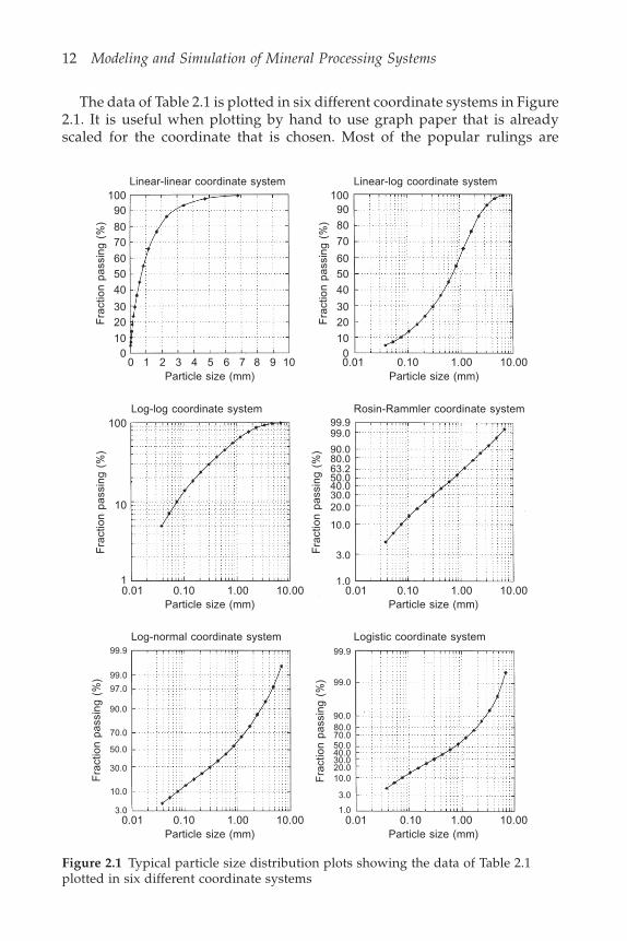
A typical set of data measured in the laboratory is shown in Table 2.1.
Table 2.1 A typical set of data that defines the particle sizedistribution of a population of particles
Mesh size (mm) Mass % passing
6.80 99.54.75 97.53.40 93.32.36 86.41.70 76.81.18 65.80.850 55.00.600 45.10.425 36.70.300 29.60.212 23.50.150 18.30.106 13.90.075 10.00.053 7.10.038 5.0
12 Modeling and Simulation of Mineral Processing Systems
The data of Table 2.1 is plotted in six different coordinate systems in Figure2.1. It is useful when plotting by hand to use graph paper that is alreadyscaled for the coordinate that is chosen. Most of the popular rulings are
Figure 2.1 Typical particle size distribution plots showing the data of Table 2.1plotted in six different coordinate systems
10090
8070
6050
40
3020
100
Fra
ctio
n pa
ssin
g (%
)
0 1 2 3 4 5 6 7 8 9 10
10090
80
70
6050
40
3020
100
Fra
ctio
n pa
ssin
g (%
)
Particle size (mm)0.01 0.10 1.00 10.00
Particle size (mm)
Linear-linear coordinate system Linear-log coordinate system
100
10
1
Log-log coordinate system Rosin-Rammler coordinate system
0.01 0.10 1.00 10.00Particle size (mm)
0.01 0.10 1.00 10.00Particle size (mm)
99.999.0
90.080.063.250.040.030.020.0
10.0
3.0
1.0
0.01 0.10 1.00 10.00Particle size (mm)
0.01 0.10 1.00 10.00Particle size (mm)
Fra
ctio
n pa
ssin
g (%
)
Fra
ctio
n pa
ssin
g (%
)
99.9
99.0
90.080.070.050.040.030.020.010.0
3.0
1.0
Fra
ctio
n pa
ssin
g (%
)
99.9
99.0
90.0
70.0
50.0
30.0
10.0
3.0
Fra
ctio
n pa
ssin
g (%
)
Log-normal coordinate system Logistic coordinate system
97.0
Particle populations and distribution functions 13
readily available commercially. It is even more convenient to use a computergraph plotting package such as the PSD program on the companion CD thataccompanies this text and which offers all of the coordinate systems shownas standard options.
2.3 The distribution density functionIn much of the theoretical modeling work it will be convenient to work witha function that is derived from the distribution function by differentiation.Let x represent any particle characteristic of interest. Then P(x) is the massfraction of the particle population that consists of particles having the valueof the characteristic less than or equal to x. The distribution density functionp(x) is defined by
p x dP xdx
( ) = ( ) (2.24)
The discrete density function defined in Equation 2.1 is related to the densityfunction by
p p x dxiD
D
i
i
= ( )–1
= P(Di–1) – P(Di) (2.25)
A usual but imprecise interpretation of the distribution density function isthat p(x)dx can be regarded as the mass fraction of the particle populationthat consists of particles having the value of the characteristic in the narrowrange (x, x + dx).
An important integral relationship is
0( ) = ( ) – (0) = 1p x dx P P (2.26)
which reflects that the sum of all fractions is unity.
2.4 The distribution by number, the representativesize and population averages
Because all particle populations contain a finite number of particles it is alsopossible to describe the variation of particle characteristics through the numberfraction. The number distribution function for any characteristic (having valuesrepresented by the variable x) is defined as the function (x) which is thefraction by number of particles in the population having size equal to x orless. The associated number density function is defined by
= ( )d xdx
(2.27)

14 Modeling and Simulation of Mineral Processing Systems
The discrete number density is given by
i = (Xi–1) – (Xi) = i (2.28)
where the upper case letters represent the class boundaries.Often it is useful to have average values for any characteristic with the
average taken over all members of the population. The average value of anycharacteristic property is given by
xN
xNT j
Nj
T
= 1=1
( ) (2.29)
where x(j) is the value of the characteristic property for particle j and NT is thetotal number of particles in the population. Equation 2.29 is unwieldy becausethe summation must be taken over a very large number, NT, of particles. Thenumber of terms in the summation is greatly reduced by collecting particlesthat have equal values of x into distinct groups. If the number of particles ingroup i is represented by n(i) and the value of x for particles in this group isrepresented by xi, then the average value of the property x in the wholepopulation is given by
xN
n xNT i
Ni
i= 1=1
( ) (2.30)
where N represents the total number of groups that are formed. The ration(i)/NT is the fraction by number of the particle population having size xi.This allows an alternative and even more convenient way of evaluating theaverage
x xN i
N
i i==1
(2.31)
Other averages are sometimes used. For example the average could be weightedby particle mass rather than by number
xM
m xT i
Ni
i = 1=1
( ) (2.32)
In Equation 2.32 MT represents the total mass of material in the populationand m(i) the mass of particles in the group i having representative value xi.The ratio m(i)/MT is the fraction by mass of particles in the group i and thisis related to the distribution function
mM
P x P x P pi
Ti i i i
( )+1 = ( ) – ( ) = = (2.33)
x x Pi
N
i i = =1
(2.34)
= ( )=1i
N
i ix p x (2.35)
Particle populations and distribution functions 15
In the limit as the group widths decrease to zero, Equation 2.34 becomes
x x dP x = ( )0
1
(2.36)
= ( ) 0
xp x dx (2.37)
In a similar way the variance of the distribution can be obtained
2
0
2 = ( – ) ( ) x x p x dx (2.38)
The distribution density function is useful for the evaluation of the averageof any function of the particle property x.
f x f x p x dx( ) = ( ) ( ) 0
(2.39)
In the same way, the average value of the property, x, weighted by number isobtained from
x x x dxN = ( ) 0
(2.40)
or more generally
f x f x x dxN( ) = ( ) ( ) 0
(2.41)
For example, if all particles in the population are spherical, the average particle
volume is the average value of dp3/6 . Thus
Average particle volume = 0
3
6 ( )
dd dd
pp p (2.42)
In order that it is possible to describe the behavior of the particles adequately,the concept of a representative size for each size class is introduced. Arepresentative size for size class i is defined through the expression
dd
d d ddpii p D
D
p p pi
i3 3 = 1
( ) ( )
–1
(2.43)
where (dp) is the number distribution density function and i(dp) is thenumber fraction of the population in size class i. Other definitions of therepresentative size can be used and the precise definition will depend on thecontext in which the representative size will be used. It is important that therepresentative size be such that a single particle having the representativesize would behave in a way that will adequately represent all particles in theclass.

16 Modeling and Simulation of Mineral Processing Systems
It is also possible to estimate the representative size from
dp
d p d ddpii D
D
p p pi
i
= 1 ( ) –1
= 1 ( )–1
pd dP d
i D
D
p pi
i
(2.44)
which weights the individual particles in the class by mass.These two definitions of the representative size require the size distribution
function to be known before the representative size can be established. Inmany circumstances this will be unsatisfactory because it would be moreconvenient to have the size classes together with their representative sizesdefined independently of the size distribution. A common method is to usethe geometric mean of the upper and lower boundaries for the representativesize.
dpi = (DiDi–1)1/2 (2.45)
Since DN = 0 and D0 is undefined, Equation 2.45 cannot be used to calculatethe representative sizes in the two extreme size classes. These sizes are calculatedusing
dd
d
dd
d
pp
p
pNpN
pN
12
2
3
–12
– 2
=
=
(2.46)
These formulas project the sequence dpi as a geometric progression into thetwo extreme size classes.
The arrangements of mesh and representative sizes is shown in Figure 2.2.
Nd pN
d pN – 1d pN – 2
N – 1 N–2
DN DN–1DN–2 DN–3 D4 D3 D2 D1
Particle size
Mesh size
Size class
Representativesize
d p2d p3
d p4
4 3 2
Figure 2.2 Arrangement of class sizes, representative sizes and mesh sizes alongthe particle size axis
2.5 Distributions based on particle compositionThe mineralogical composition of the particles that are processed in ore dressingoperations varies from particle to particle. This is of fundamental importance

Particle populations and distribution functions 17
in any physical separation process for particulate material. The primaryobjective of ore dressing processes is the separation of materials on the basisof mineralogical composition to produce concentrates having a relativeabundance of the desired mineral. The objective of comminution operationsis the physical separation of minerals by fragmentation. Unfortunately, exceptin favorable cases, the minerals do not separate completely and many particles,no matter how finely ground, will contain a mixture of two or more mineralspecies. Some particles will, however, always exist that are composed of asingle mineral. These are said to be perfectly liberated. The amount of mineralthat is liberated is a complex function of the crystalline structure andmineralogical texture of the ore and the interaction between these and thecomminution fracture pattern.
The mineralogical composition of a particle can be unambiguously definedby the fractional composition of the particle in terms of the individual mineralcomponents that are of interest. Generally, more than one mineral speciesmust be accounted for so that the mineralogical composition is described bya vector g of mineral fractions. Each element of the vector g represents the massfraction of a corresponding mineral in the particle. The number of elementsin the vector is equal to the number of minerals including gangue minerals.Thus in a particle that is made up of 25% by mass of chalcopyrite, 35% ofsphalerite and 40% of gangue would be described by a mineral fraction vectorg = (0.25 0.35 0.40). A number of discrete classes of mineral fractions can bedefined and the range of each element fraction, i.e. the range of each componentof the vector g, must be specified for each class of particles. The fractionaldiscrete distribution function can be defined as was done for particle size.
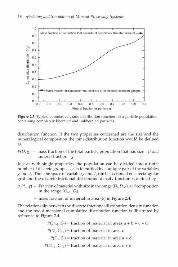
A special class exists for mineral fractions at the extreme ends of thecomposition range. In ore dressing operations it is usual to work with particlepopulations that have some portion of the mineral completely liberated. Thusa definite non-zero fraction of the particle population can have a mineralfraction exactly equal to zero or unity and a separate class is assigned to eachof these groups of particles. These classes have class widths of zero. If only asingle valuable mineral is considered to be important, g is a scalar and thedistribution function P(g) will have the form shown in Figure 2.3.
The concentration of particles in the two extreme classes representingcompletely liberated gangue and mineral respectively is represented by thestep discontinuities in the distribution functions. When more than one mineralis significantly important, the simple graphical representation used in Figure2.3 is no longer available and a multidimensional description is required.
2.6 Joint distribution functionsIt often happens that more than one property of the particle is significant ininfluencing its performance in an ore dressing operation. In that case it isessential to use a description of the particle population that takes all relevantproperties into account. The appropriate description is provided by the joint
18 Modeling and Simulation of Mineral Processing Systems
distribution function. If the two properties concerned are the size and themineralogical composition the joint distribution function would be definedas
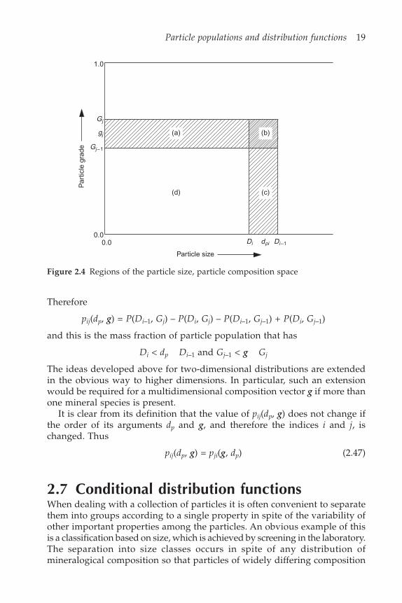
P(D, g) = mass fraction of the total particle population that has size D andmineral fraction g.
Just as with single properties, the population can be divided into a finitenumber of discrete groups – each identified by a unique pair of the variablesg and dp. Thus the space of variable g and dp can be sectioned on a rectangulargrid and the discrete fractional distribution density function is defined by
pij(dp, g) = Fraction of material with size in the range (Di, Di–1), and compositionin the range (Gj–1, Gj)
= mass fraction of material in area (b) in Figure 2.4.
The relationship between the discrete fractional distribution density functionand the two-dimensional cumulative distribution function is illustrated byreference to Figure 2.4.
P(Di–1, Gj) = fraction of material in areas a + b + c + d
P(Di, Gj–1) = fraction of material in area d
P(Di, Gj) = fraction of material in area a + d
P(Di–1, Gj–1) = fraction of material in area c + d
Figure 2.3 Typical cumulative grade distribution function for a particle populationcontaining completely liberated and unliberated particles
Mass fraction of population that consists of completely liberated mineral
1.0
0.9
0.8
0.7
0.6
0.5
0.4
0.3
0.2
0.1
0.00.0 0.1 0.2 0.3 0.4 0.5 0.6 0.7 0.8 0.9 1.0
Mass fraction of population that consists of completely liberated gangue
Mineral fraction in particle g
Cum
ulat
ive
dist
ribut
ion
P(g
)
Particle populations and distribution functions 19
Therefore
pij(dp, g) = P(Di–1, Gj) – P(Di, Gj) – P(Di–1, Gj–1) + P(Di, Gj–1)
and this is the mass fraction of particle population that has
Di < dp Di–1 and Gj–1 < g Gj
The ideas developed above for two-dimensional distributions are extendedin the obvious way to higher dimensions. In particular, such an extensionwould be required for a multidimensional composition vector g if more thanone mineral species is present.
It is clear from its definition that the value of pij(dp, g) does not change ifthe order of its arguments dp and g, and therefore the indices i and j, ischanged. Thus
pij(dp, g) = pji(g, dp) (2.47)
2.7 Conditional distribution functionsWhen dealing with a collection of particles it is often convenient to separatethem into groups according to a single property in spite of the variability ofother important properties among the particles. An obvious example of thisis a classification based on size, which is achieved by screening in the laboratory.The separation into size classes occurs in spite of any distribution ofmineralogical composition so that particles of widely differing composition
Figure 2.4 Regions of the particle size, particle composition space
Par
ticle
gra
de
Particle size
(a) (b)
(d) (c)
1.0
Gj
gj
Gj–1
0.00.0 Di dpi Di–1
20 Modeling and Simulation of Mineral Processing Systems
will be trapped on the same test sieve. Each batch of material on the differenttest sieves will have a different distribution of compositions. For example,the batch of particles in the finest size class will be relatively rich in completelyliberated material. There is a unique composition distribution function foreach of the size classes. The screening is called a conditioning operation andthe distribution function for each size class is called a conditional fractionaldistribution function.
The conditional discrete density function pji(g |dp) is defined as the massfraction of the particles in size class i (i.e. have size between Di and Di–1), thatare in composition class j. These conditional distribution functions can berelated to the joint distribution functions that have already been defined.
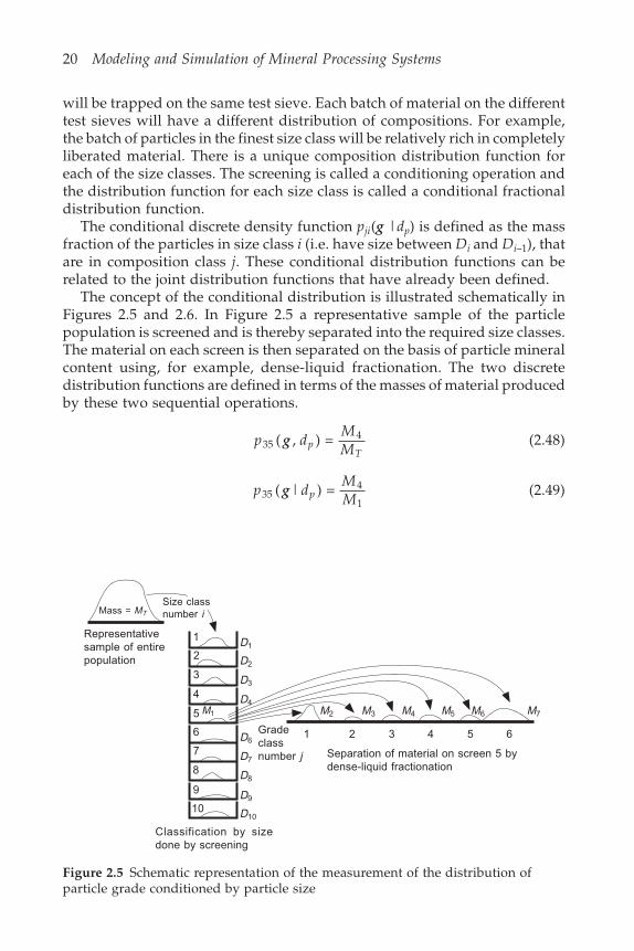
The concept of the conditional distribution is illustrated schematically inFigures 2.5 and 2.6. In Figure 2.5 a representative sample of the particlepopulation is screened and is thereby separated into the required size classes.The material on each screen is then separated on the basis of particle mineralcontent using, for example, dense-liquid fractionation. The two discretedistribution functions are defined in terms of the masses of material producedby these two sequential operations.
p dMMp
T35
4( , ) = g (2.48)
p dMMp35
4
1( | ) = g (2.49)
Mass = MT
Size classnumber i
1
2
3
4
5
6
7
8
9
10
D1
D2
D3
D4
D6
D8
D9
D10
D7
Gradeclassnumber j
M2 M3 M4 M5 M6 M7
1 2 3 4 5 6
Separation of material on screen 5 bydense-liquid fractionation
Classification by sizedone by screening
Representativesample of entirepopulation
M1
Figure 2.5 Schematic representation of the measurement of the distribution ofparticle grade conditioned by particle size
Particle populations and distribution functions 21
M1
M 2
M 3
M 4
M 5
M 6
M 7
M 8
M 9
M10
M11
and
p dMMp
T5
1( ) = (2.50)
It is easy to see that
p dMM
M MM M
p dp dp
T
T
p
p35
4
1
4
1
35
5( | ) = =
//
= ( , )( )
gg
(2.51)
and that pj5( g|dp) shows how the material on screen 5 is distributed withrespect to the particle composition.
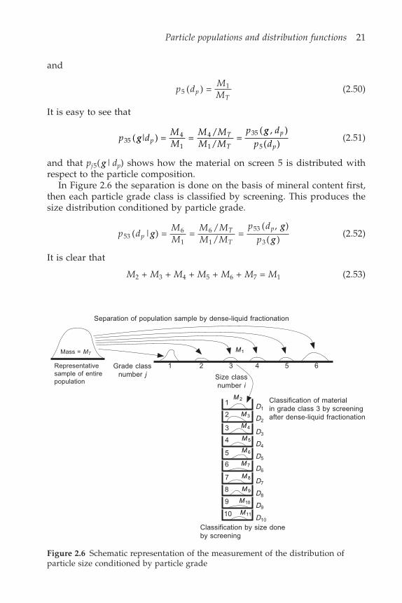
In Figure 2.6 the separation is done on the basis of mineral content first,then each particle grade class is classified by screening. This produces thesize distribution conditioned by particle grade.
p dMM
M MM M
p dpp
T
T
p53
6
1
6
1
53
3( | ) = =
//
= ( , )
( )g
gg
(2.52)
It is clear that
M2 + M3 + M4 + M5 + M6 + M7 = M1 (2.53)
Figure 2.6 Schematic representation of the measurement of the distribution ofparticle size conditioned by particle grade
Mass = MT
Representativesample of entirepopulation
1
2
3
4
5
6
7
8
9
10
D1
D2
D3
D4
D6
D8
D9
D10
D7
Grade classnumber j
1 2 3 4 5 6
Classification by size doneby screening
D5
Classification of materialin grade class 3 by screeningafter dense-liquid fractionation
Separation of population sample by dense-liquid fractionation
Size classnumber i
22 Modeling and Simulation of Mineral Processing Systems
so that
j ji pp d=1
6
( | ) = 1g (2.54)
and
j j p pp d p d=1
6
5 5 ( , ) = ( )g (2.55)
These ideas can be generalized to develop the following relationships. If M isthe mass of the total population, the mass of particles that fall in the twoclasses j and i simultaneously is just Mpji(g, dp). When this is expressed as afraction of only those particles in the dp class, namely Mpi(dp), the conditionaldistribution is generated.
Thus
p dMp d
Mp d
p dp d
ji pji p
i p
ji p
i p
( | ) = ( , )( )
= ( , )( )
gg
g(2.56)
Equation 2.56 is important chiefly because it provides a means for thedetermination of the theoretically important joint discrete distribution functionpji(g, dp) from the experimentally observable conditional distribution functionpji(g | dp)
pji(g, dp) = pji(g|dp)pi(dp) (2.57)
Since
pji(g, dp) = pij(dp, g) (2.58)
we note that
pji(g, dp) = pij(dp|g)pj (g) (2.59)
and
pji(g|dp)pi(dp) = pij(dp|g)pj (g) (2.60)
Equation 2.57 corresponds to an experimental procedure in which the particlepopulation is first separated on the basis of size by screening followed by aseparation of each screened fraction into various composition groups. Equation2.60 on the other hand corresponds to a separation on the basis of composition(by magnetic, electrostatic, or dense liquid techniques perhaps) followed bya sieve analysis on each composition class. Either way the same joint distributionfunction is generated but the former experimental procedure is in most instancesmuch less convenient than the latter because of the experimental difficultiesassociated with separation by composition. It is usually more efficient to
Particle populations and distribution functions 23
combine one composition separation with many size separations (which arecomparatively simple to do in the laboratory) than the other way about.
The density functions satisfy the following general relationships whichmay be verified using the same simple principles that are used above.
i j ijp x y ( , ) = 1 (2.61)
j ij j ij j ip x y p x y p y p x ( , ) = ( | ) ( ) = ( ) (2.62)
i ij i ji i jp x y p y x p x p y ( , ) = ( | ) ( ) = ( ) (2.63)
i ijp x y ( | ) = 1 (2.64)
The principles developed in this section can be used to define the conditionaldistribution functions P(g|dp) and P(g| dp) as well as the associated densityfunctions p(g|dp). These are related by
p x ydP x y
dx( | ) =
( | )(2.65)
p x yp x y
p y( | ) =
( , )( )
(2.66)
and satisfy the following relationships analogous to Equations 2.61–64.
p x y dx dy( , ) = 1 (2.67)
p x y dy p x( , ) = ( ) (2.68)
p x y dx p y x p x dx p y( , ) = ( | ) ( ) = ( ) (2.69)
p x y dx( | ) = 1 (2.70)
2.7.1 Practical representations of conditional gradedistributions – the washability curve
Conditional grade distributions have been used for many years in practicalmineral processing and a number of standard representational methods haveevolved. Of these, the most widely used is the washability distribution andthe associated washability curve. This method was developed initially toanalyze coal washing operations and it is based on the dense-liquid fractionationlaboratory method. This procedure is based on the use of a sequence oforganic liquids having different densities usually in the range 1200 kg/m3 toabout 3200 kg/m3 although denser liquids can be synthesized and used. The
24 Modeling and Simulation of Mineral Processing Systems
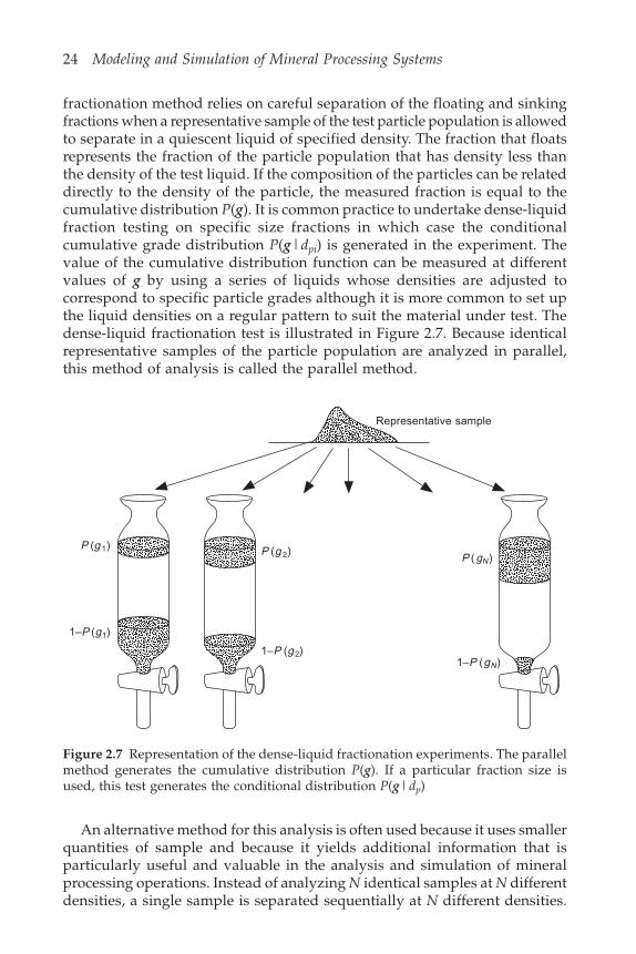
fractionation method relies on careful separation of the floating and sinkingfractions when a representative sample of the test particle population is allowedto separate in a quiescent liquid of specified density. The fraction that floatsrepresents the fraction of the particle population that has density less thanthe density of the test liquid. If the composition of the particles can be relateddirectly to the density of the particle, the measured fraction is equal to thecumulative distribution P(g). It is common practice to undertake dense-liquidfraction testing on specific size fractions in which case the conditionalcumulative grade distribution P(g|dpi) is generated in the experiment. Thevalue of the cumulative distribution function can be measured at differentvalues of g by using a series of liquids whose densities are adjusted tocorrespond to specific particle grades although it is more common to set upthe liquid densities on a regular pattern to suit the material under test. Thedense-liquid fractionation test is illustrated in Figure 2.7. Because identicalrepresentative samples of the particle population are analyzed in parallel,this method of analysis is called the parallel method.
Representative sample
P (g 1)
1–P (g1)
P (g 2)
1–P (g2)
P (gN)
1–P (gN)
Figure 2.7 Representation of the dense-liquid fractionation experiments. The parallelmethod generates the cumulative distribution P(g). If a particular fraction size isused, this test generates the conditional distribution P(g|dp)
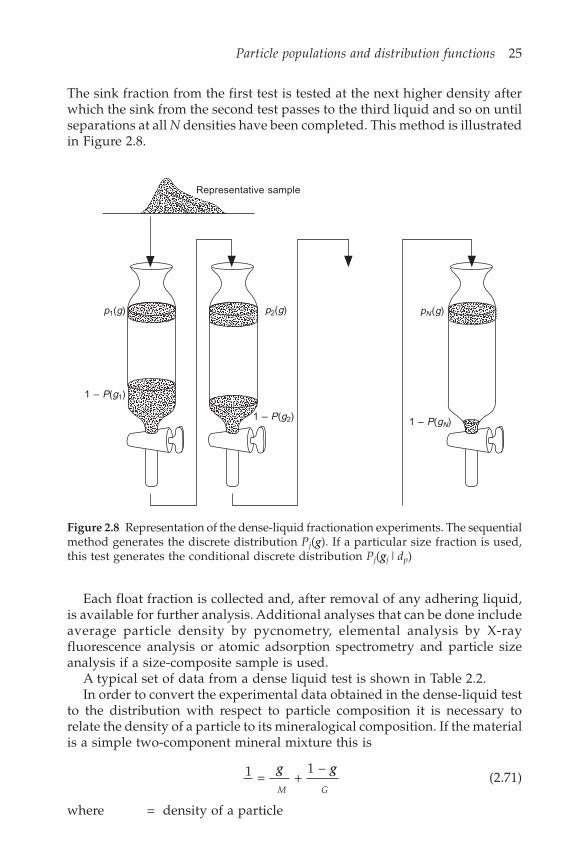
An alternative method for this analysis is often used because it uses smallerquantities of sample and because it yields additional information that isparticularly useful and valuable in the analysis and simulation of mineralprocessing operations. Instead of analyzing N identical samples at N differentdensities, a single sample is separated sequentially at N different densities.
Particle populations and distribution functions 25
The sink fraction from the first test is tested at the next higher density afterwhich the sink from the second test passes to the third liquid and so on untilseparations at all N densities have been completed. This method is illustratedin Figure 2.8.
Representative sample
p1(g)
1 – P(g1)
p2(g)
1 – P(g2)
pN(g)
1 – P(gN)
Figure 2.8 Representation of the dense-liquid fractionation experiments. The sequentialmethod generates the discrete distribution Pj(g). If a particular size fraction is used,this test generates the conditional discrete distribution Pj(gj|dp)
Each float fraction is collected and, after removal of any adhering liquid,is available for further analysis. Additional analyses that can be done includeaverage particle density by pycnometry, elemental analysis by X-rayfluorescence analysis or atomic adsorption spectrometry and particle sizeanalysis if a size-composite sample is used.
A typical set of data from a dense liquid test is shown in Table 2.2.In order to convert the experimental data obtained in the dense-liquid test
to the distribution with respect to particle composition it is necessary torelate the density of a particle to its mineralogical composition. If the materialis a simple two-component mineral mixture this is
1 = + 1 –g g
M G(2.71)
where = density of a particle
26 Modeling and Simulation of Mineral Processing Systems
M = density of the mineral phaseG = density of the gangue phaseg = mass fraction of mineral in the particle
The inverse of this equation is more useful
g = –
–G
G M
M (2.72)
which shows that the mineral grade is a linear function of the reciprocal ofthe particle density.
When the mineralogical texture is more complex than the simple binarymixture of two minerals, additional information is required from the dense-medium test to relate the particle composition to the separating density. Thisusually requires elemental analysis of the individual fractions that are obtainedin the sequential dense-liquid test. Typical data are shown in Table 2.2. Fromthe measured assays, the average mineralogical composition of particles ineach fraction can be estimated. In this case the calcite content is estimatedfrom the CaO assay and the magnesite content is estimated by differenceassuming that only the three minerals magnesite, calcite and silica are present.The relationship between the particle density and its mineralogical compositionis
–1=1
–1 = m
M
m mg (2.73)
If the density intervals used in the dense-liquid test are narrow it is reasonableto postulate that the average density of the particles in each density fractionis the midpoint between the end points of the intervals.
The densities calculated from the mineralogical compositions and the knowndensities of the minerals should correspond quite closely with the midpointdensities as shown in Table 2.3.
In the case of coal, it is usual to measure the ash content and sulfur contentof the washability fractions. It is also customary to measure the energy contentof the fractions as well because this plays a major role in assessing the utilityof the coal for power generation. Even greater detail regarding the make-up
Table 2.2 Typical data from a dense-liquid test on magnesite ore
Liquid specific Total mass yield in this % CaO % SiO2gravity fraction %
Float at 2.85 21.6 19.30 18.22.85–2.88 5.70 21.76 2.492.88–2.91 3.20 10.15 1.522.91–2.94 0.90 9.67 2.922.94–2.96 7.60 2.95 3.892.96–3.03 61.0 0.96 2.55Sink at 3.03 0.00
Particle populations and distribution functions 27
of the coal can be obtained if the full proximate analysis is determined foreach washability fraction. It is also possible to distinguish organically boundsulfur from pyritic sulfur in the coal. The greater the detail of the analysis ofthe washability fractions, the greater the detail in the products that can becalculated by modeling and simulation. These analyses are done on theseparated fractions and therefore give values that are conditional on theparticle density. This is a useful approach because many coal processingmethods separate the particles on the basis of their density. The conditionalanalyses can then be used to calculate compositions and heating values of thevarious products of the separation.
2.7.2 Measurement of grade distributions byimage analysis
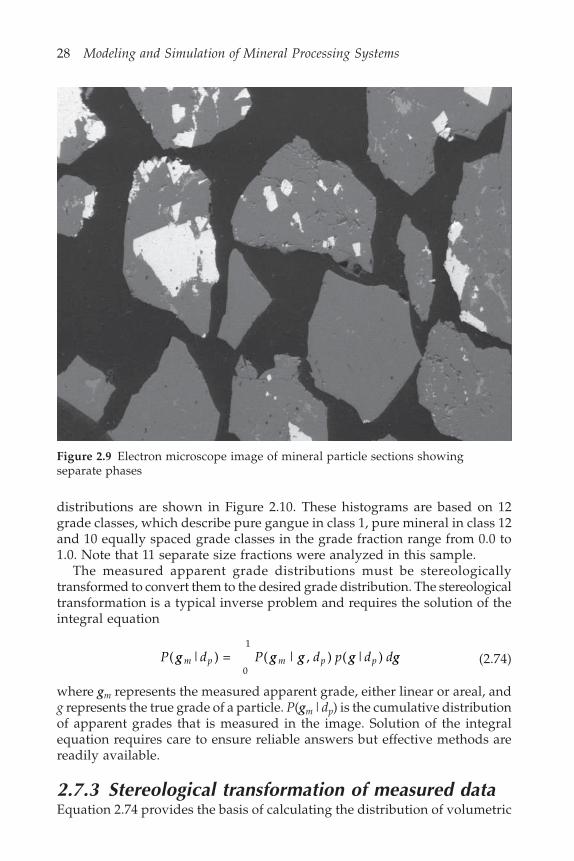
In recent years a more direct method of measurement has been developed,namely mineral liberation measurement using automatic image analysis. Thistechnique provides a direct measurement of the distribution of particle gradesin a sample from a narrow size fraction. The technique requires the generationof microscopic images of the particles that are mounted in random orientationand sectioned. The images which can be generated by optical or scanningelectron microscopy must distinguish each mineral phase that is to be measured.A typical image of a binary mineral system is shown in Figure 2.9. The apparentgrade of each particle section in the image can be readily determined whenthe image is stored in digital form. The apparent areal grade of a particlesection is the ratio of mineral phase pixels to total pixels in the section. Figure2.9 is typical of images obtained from mineral particles that are collected inmineral processing plants and it is easy to see that the lack of liberation willhave a profound effect on the unit operations that are used to upgrade themineral species.
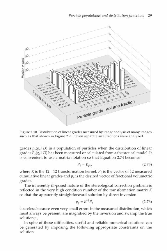
Alternatively the apparent grade of many linear intercepts across a particlesection can be measured. It is a simple matter to establish the distribution ofapparent linear or areal grades from images containing a sufficiently largenumber of particle sections. Typical histograms of measured linear grade
Table 2.3 Data derived from the measured data in Table 2.2
Liquid specific Magnesite Calcite (%) SiO2 (%) Calculated densitygravity (%) (kg/m3)
Float at 2.85 47.34 34.46 18.2 28282.85–2.88 58.65 38.86 2.49 28672.88–2.91 80.36 18.13 1.52 29352.91–2.94 79.81 17.28 2.92 29332.94–2.96 90.85 5.26 3.89 29682.96–3.03 95.74 1.71 2.55 2985Sink at 3.03
28 Modeling and Simulation of Mineral Processing Systems
distributions are shown in Figure 2.10. These histograms are based on 12grade classes, which describe pure gangue in class 1, pure mineral in class 12and 10 equally spaced grade classes in the grade fraction range from 0.0 to1.0. Note that 11 separate size fractions were analyzed in this sample.
The measured apparent grade distributions must be stereologicallytransformed to convert them to the desired grade distribution. The stereologicaltransformation is a typical inverse problem and requires the solution of theintegral equation
P d P d p d dm p m p p( | ) = ( | , ) ( | ) 0
1
g g g g g (2.74)
where gm represents the measured apparent grade, either linear or areal, andg represents the true grade of a particle. P(gm|dp) is the cumulative distributionof apparent grades that is measured in the image. Solution of the integralequation requires care to ensure reliable answers but effective methods arereadily available.
2.7.3 Stereological transformation of measured dataEquation 2.74 provides the basis of calculating the distribution of volumetric
Figure 2.9 Electron microscope image of mineral particle sections showingseparate phases
Particle populations and distribution functions 29
grades pv(gv|D) in a population of particles when the distribution of lineargrades P�(g�|D) has been measured or calculated from a theoretical model. Itis convenient to use a matrix notation so that Equation 2.74 becomes
P� = Kpv (2.75)
where K is the 12 12 transformation kernel. P� is the vector of 12 measuredcumulative linear grades and pv is the desired vector of fractional volumetricgrades.
The inherently ill-posed nature of the stereological correction problem isreflected in the very high condition number of the transformation matrix Kso that the apparently straightforward solution by direct inversion
pv = K–1P� (2.76)
is useless because even very small errors in the measured distribution, whichmust always be present, are magnified by the inversion and swamp the truesolution pv.
In spite of these difficulties, useful and reliable numerical solutions canbe generated by imposing the following appropriate constraints on thesolution
Figure 2.10 Distribution of linear grades measured by image analysis of many imagessuch as that shown in Figure 2.9. Eleven separate size fractions were analyzed
30 Modeling and Simulation of Mineral Processing Systems
i vip
=1 = 1.0
12
(2.77)
and
pvi 0 for i = 1, 2 . . . 12 (2.78)
with pvi representing the ith element of the vector pv.
The solution is obtained by imposing additional regularization conditionswhich reflect the relative smoothness that would be expected for the distributionfunction pv(g|D) in any real sample of ore, and the transformed distributionis obtained as the solution to the constrained minimization problem
Minimize ||100( – )|| + ln
=1
12
pv i v
ivi
vi
Kp P p pl (2.79)
subject to equality constraint 2.77 and inequalities 2.78. The term –i v
ivip p
=1
12
ln
measures the entropy of the distribution pvi and increases as the distribution
becomes smoother.The regularization parameter in Equation 2.79 is arbitrary and controls
the weight given to maximization of the entropy of the distribution relativeto minimization of the residual norm. Large favors larger entropy andtherefore smoother solutions at the cost of larger residual norms. In practicea value of = 1.0 has been found to be a satisfactory choice in most cases.
In general the kernel matrix should be determined separately for everysample that is analyzed but this is a time-consuming and tedious task. As aresult users of this method develop libraries of kernel matrices from whichthe most appropriate can be selected for a particular application. A usefulkernel that will produce good results for many ores is
P g g v� �( | )
=
!∀#### #∀∃!%##∀&&#∃#∀∋(&∃ #∀)∗∋∋ #∀!%#&#∀!+!! #∀!#+! #∀#()( #∀#+∋∋ #∀#!++ #∀####
!∀#### #∀%#)∃#∀∗%∗##∀&!#! #∀∋∗+# #∀)&(! #∀!∃#%#∀!)&+ #∀#∃)∗ #∀#+(# #∀#!&! #∀####
!∀#### #∀%)∃∃#∀(∗+&#∀&%∃(#∀+&)! #∀∋∋!∃ #∀)∋∗( #∀!∗)! #∀!#∋∋ #∀#&∗! #∀#!(! #∀####
!∀#### #∀%+∗##∀∃!+%#∀∗(!∗ #∀&∋)%#∀+#∃) #∀∋##) #∀)#∃( #∀!∋)+ #∀#(#! #∀#)#& #∀####
!∀#### #∀%&∃+#∀∃&+∋#∀(∋∋+ #∀∗#(∋ #∀+∃+∋ #∀∋∗∃∃ #∀)∗∋) #∀!∗%∋ #∀#∃%+#∀#)&&#∀####
∀ #∀%∗(( #∀∃∃&( #∀(∃∗! #∀∗(&∋ #∀&&%##∀++!# #∀∋)+( #∀)!∋% #∀!!+∋ #∀#∋)∋ #∀####
!∀#### #∀%(+&#∀%!#∗ #∀∃∋#( #∀(∋∗∃ #∀∗∋!) #∀&!&(#∀∋%)( #∀)∗∗∗ #∀!+&( #∀#+!∗ #∀####
!∀#### #∀%(%&#∀%)%%
1 0000
#∀∃∗(∗#∀∃∗(∗ #∀(%!∋ #∀∗%%∃#∀&%!∃#∀+∗(! #∀∋)∃+ #∀!∃&! #∀#&+##∀####
!∀#### #∀%∃)%#∀%+∋%#∀∃%∗(#∀∃∋(% #∀(∗∋∋ #∀∗∗∃) #∀&+(%#∀+#!∋ #∀)∋&&#∀#(!) #∀####
!∀#### #∀%∃+%#∀%&∋##∀%!(+ #∀∃(+∗ #∀∃!%! #∀(+)% #∀∗∋∗# #∀+∃%%#∀∋#+# #∀#%() #∀####
!∀#### #∀%∃&∗#∀%&∗(#∀%)(∋ #∀∃%&%#∀∃&∃%#∀∃#%&#∀(∋∗( #∀∗)+) #∀++%)#∀!∃!# #∀####
!∀#### !∀#### !∀#### !∀#### !∀#### !∀#### !∀#### !∀#### !∀#### !∀#### !∀#### !∀####
(2.80)

Particle populations and distribution functions 31
A histogram of the true volumetric distribution of particle grades is shown inFigure 2.11 after stereological correction of the data in Figure 2.10. Theimportance of transforming the data is immediately apparent from thesefigures. The untransformed data do not reveal the true nature of the liberationdistribution and cannot be used to analyze the behavior of individual particletypes in any mineral processing operation. This should be borne in mindwhen experimental image analysis data is to be used for model calibrationpurposes.
Figure 2.11 Liberation distributions of 11 particle size fractions of a 2-component oremeasured by image analysis. These histograms were obtained by stereologicaltransformation of the data shown in Figure 2.10
2.8 IndependenceIt happens that sometimes two properties can be distributed independentlyof each other. This idea can be made precise by defining the independence oftwo properties, say k and dp, if the following relationship is satisfied.
pji(k|dp) = pj(k) (2.81)
which means that the distribution of k values (these could be flotation rateconstants for example) is the same within any size class as it is across theentire population.
32 Modeling and Simulation of Mineral Processing Systems
This leads to
pji(k, dp) = pj(k|dp)pi(dp)
= pj(k)pi(dp) (2.82)
which shows that the joint distribution for two properties that are independentcan be generated as the product of the two separate distribution functions.
2.9 Distributions by numberIn some situations it is useful to use number fractions rather than mass fractionswhen dealing with particle populations. The relationship between the massdistribution functions and the equivalent number distribution function canbe deduced as follows.
The number distribution function (dp) is defined to be equal to the numberfraction of particles in the entire population with size dp. Number distributionfunctions and number distribution density functions can be defined in asimilar way for each of the distribution types already defined for mass fractions.In particular the discrete number fractional distribution function is definedby
i p
i p
d
n dN
( ) = number of particles in size class i
Total number of particles in the population
( )
(2.83)
The number distributions can be related to the mass distributions as follows
Let (m)dm = number fraction of particles having mass in (m, m + dm)(m|dp)dm = number fraction of particles of size dp that have mass in
(m, m + dm). That is the distribution density for particlemass conditioned by particle size
pi(dp) = mass fraction of particles in size class im = mass of a particle of size dp
m dp( ) = average mass of a particle of size dp
M = total mass of particles in the populationN = total number of particles in the population
Mp d N m m d dmp p( ) = ( , )0
= ( | ) ( )0
N m m d d dmp p (2.84)
= ( ) ( | )0
N d m m d dmp p
= ( ) ( )N d m dp p
Particle populations and distribution functions 33
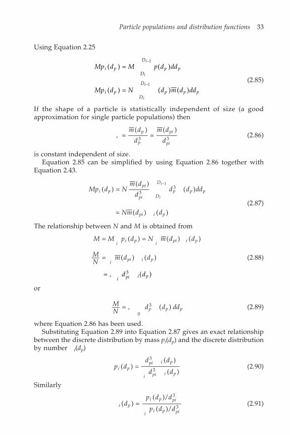
Using Equation 2.25
Mp d M p d dd
Mp d N d m d dd
i pD
D
p p
i pD
D
p p p
i
i
i
i
( ) = ( )
( ) = ( ) ( )
–1
–1(2.85)
If the shape of a particle is statistically independent of size (a goodapproximation for single particle populations) then
, = ( )
= ( )
3 3
m d
d
m d
dp
p
pi
pi
(2.86)
is constant independent of size.Equation 2.85 can be simplified by using Equation 2.86 together with
Equation 2.43.
Mp d Nm d
dd d ddi p
pi
pi D
D
p p pi
i
( ) = ( )
( )33
–1
(2.87)= ( ) ( )Nm d dpi i p
The relationship between N and M is obtained from
M M p d N m d di i p i pi i p = ( ) = ( ) ( )
MN
m d di pi i p = ( ) ( ) (2.88)
= ( )3,i pi i pd d
or
MN
d d ddp p p = ( ) 0
3, (2.89)
where Equation 2.86 has been used.Substituting Equation 2.89 into Equation 2.87 gives an exact relationship
between the discrete distribution by mass pi(dp) and the discrete distributionby number i(dp)
p dd d
d di p
pi i p
i pi i p( ) =
( )
( )
3
3 (2.90)
Similarly
i pi p pi
i i p pi
dp d d
p d d( ) =
( )/
( )/
3
3 (2.91)

34 Modeling and Simulation of Mineral Processing Systems
2.10 Internal and external particle coordinateand distribution densities
Up to now, the particles have been classified according to two very importantproperties: the particle size and the mineralogical composition. These aretwo examples of many properties that can be used to describe the particle.They are certainly the most important descriptive properties so far as oredressing and hydrometallurgical processes are concerned, but in order todevelop effective models for the unit operations it is always necessary toensure that the particles are described in sufficient detail for the purposes ofthe modeling study. It is impossible to make a complete description of anyone particle – such concepts as particle shapes, surface topography, surfaceenergy etc. cannot be completely described in a quantitative sense using afinite number of variables. Consequently, it is always necessary to choose afinite and comparatively small number of variables that can be used to describethe particle properties in sufficient detail for the purposes of the model.
The properties that describe the nature of the individual particles are calledthe internal coordinates of the particle phase space. The choice of thesecoordinates is dictated entirely by the demands of the model. However, it isalways necessary to bear in mind that one of the primary objectives of modelingthe unit operations is to link these together in a plant flowsheet so that theplant can be simulated. It will often happen that the set of internal coordinatesthat are required to model one of the unit operations might not be appropriatefor the other models. In general the problem is overcome by specifying a setof internal coordinates that will include all internal coordinates required forthe separate models as subsets. This means that some of the internal coordinateswill be redundant in some of the unit models. This does not cause any problemsin general.
In some unit operations, the physical location of the particle in the unitequipment can have a very significant effect on the particle behavior and it issometimes necessary to track the position of the particles in the equipment inorder to describe the operation of the unit as a whole. This is not alwaysnecessary but in formulating the general model structure it is convenient toinclude them.
The distribution functions that were described in Section 2.9 can be relatedto corresponding distribution density functions and it is convenient to formulatea generalized model in terms of the joint distribution density function for allthe particle coordinates external and internal.
The generalized particulate distribution density function (x) is an ordinaryfunction of the vector argument x which comprises all of the external andinternal coordinates that are relevant to the problem on hand. All possiblevectors x make up the particle phase space. (x) is defined as the numberfraction density, i.e. the number fraction of the entire particle population thatoccupies unit volume of the particle phase space. The finite particle distributionfunctions defined previously can be constructed from the distribution densityas follows.

Particle populations and distribution functions 35
In the case where the phase space consists only of the particle size (dp) andthe particle grade (g)
ij p iD
D
G
G
p pd g d g dd dgi
i
i
i
( , ) = ( , ) –1 +1
(2.92)
The mathematical description of is sometimes difficult. For example it maynot be possible to obtain in terms of any known transcendental functionsand may have to include Dirac delta functions. Particular examples are thetwo extreme ends of the liberation spectrum. Thus we tend to avoid forpractical modeling work and use it only formally to develop some necessarymodel structures.
2.11 Particle properties derived from internalcoordinates
The internal coordinates of a particle should be sufficient to describe allsignificant characteristics of the particle. In many situations it is necessary toobtain some derived quantity. Some examples are: the metal assay from themineralogical composition, the magnetic susceptibility of the particle fromthe magnetic susceptibilities of the individual minerals, and the calorificvalue, volatile content and ash content of a coal particle from the mineralmatter content plus the maceral content.
The density of the particle is a particularly important derived propertyand we note that this is related to mineralogical composition by
1 = =1m
Mm
m
g(2.93)
wherem = density of mineral phase
= density of particlegm = mass fraction of mineral phase m in the particle (particle grade).
2.12 The population balance modeling methodThe characterization of a particle population through the distribution of particlesin the external and internal variable spaces provides a powerful formalizedmodeling procedure. The essential idea is that as the particles move throughthe processing environment their external and internal coordinates change –the external coordinates because they move physically and the internalcoordinates because the particles are altered by the processing.
The collection of external and internal coordinates attached to a particledefines the coordinate location of the particle in the phase space. The externalcoordinates describe its actual physical location while the internal coordinates

36 Modeling and Simulation of Mineral Processing Systems
describe the characteristics of the particle itself. The internal coordinates mustbe sufficiently numerous to describe the particle in all the detail necessary forits complete characterization in terms of the processes that must be describedby the model.
Some examples of internal coordinates are:
− particle size; this is perhaps the most important of all− mineralogical composition− chemical composition− particle shape− surface specific energy.
Some of these internal coordinates may themselves be multidimensional. Forexample the mineralogical composition of the solid material may includemore than two minerals in which case the mineralogical composition vectormust include one coordinate for each distinct mineral. Sometimes the multi-dimensionality of the internal coordinates must be infinite. This occurs, forexample, during leaching processes when the concentration of the speciesthat is being leached varies continuously within the particle and the chemicalcomposition must be known at every point within the particle. In general theconcentration profile of the leached component will be low near the surfaceof the particle and higher further in where lixiviant has not attained highconcentrations because of diffusional resistance within the particle. Theconcentration profile is a functional of the entire processing history of theparticle. In practice it is not convenient to use an infinite-dimensional internalcoordinate and various finite-dimensional approximations must be made.An important instance when a one-dimensional internal characterization iscompletely adequate applies to the technically important topochemicalprocesses where the radial position of the topochemical interface inside theparticle often carries complete information regarding the concentration profileand its effect on the rate of the chemical process. There is a large class ofparticulate rate processes that can be modeled topochemically and for whichthe instantaneous rate of the process over the particle as a whole can bewritten as a unique function of the position of the topochemical interface.This makes topochemical models very powerful models indeed for thedescriptions of particulate rate processes. Furthermore topochemical modelspermit the calculation of the rate at which the topochemical boundary movesand this rate is important in the formulation of population balance modelsfor the particle population as a whole.
2.13 The fundamental population balanceequation
Notation used in this section:
(x)dx is the number fraction of particles per unit volume of phase space,
Particle populations and distribution functions 37
i.e. the number fraction of the particle population that occupies asmall volume around the phase coordinate x.
x is the coordinate point in phase space x . �N
u is a vector of ‘velocities’ at which particles change their phasecoordinates. For example this could be the rate of change of particlesize by attrition when particle size is an internal coordinate, the rateof movement of the topochemical interface when the position of theinterface is the internal coordinate or the rate of change of particlecomposition when the particle undergoes chemical change. Thecorresponding elements for the external coordinate are the physicalvelocities in three-dimensional space.
�(x) is the rate at which particles at coordinate position x are destroyed.This rate is specified as mass per unit volume of phase space perunit time.
Win is the mass rate at which solid material is fed to the system.Wout is the mass rate at which solid material is withdrawn from the
system.The material in the feed and product is distributed in the phasespace according to in and out respectively.
m( )x is the average mass of a particle at point x in the phase space.N is the total number of particles in the system.A, B, D are rates of addition, birth and destruction of particles.Q is the rate of removal material through product removal streams.
B(x; x ) is a distribution function that describes the way material can movesuddenly over discrete distances in phase space following physical destructionor breakage. B(x; x ) is the mass fraction of solid material that has a phasecoordinate less then x after destruction of a particle at phase coordinate x .The statement that the phase coordinate of a particle is less than x must beinterpreted to mean that every phase coordinate of the particle is less thanthe corresponding element of x. b(x; x ) is the corresponding density function.
a(x; x ) is the distribution density for particles produced by attrition andother surface wear processes at x .
In general a(x; x ) and b(x; x ) are significantly different from each otherand in practical applications each needs to be determined separately.
Consider a region Rc of the particle phase space and account for theaccumulation of particulate mass in Rc by all processes that change thecoordinates of particles. The region Rc is completely enclosed by a surface Sc.
These processes are
1. Movement across the boundaries of Rc (convective motion in phasespace).
2. Arrivals by finite steps from other regions in the phase space.3. Destruction of particles in region Rc.4. Physical additions and withdrawals in feed and product streams.
An accounting of individual particles in the reference region Rc gives:

38 Modeling and Simulation of Mineral Processing Systems
// t
N d N d D B Q AR Sc c
( ) = – ( ) – + – + x x x u . n (2.94)
In this equation, n is the outward pointing normal vector to the surface Sc atpoint x.
In our mineral processing systems solid mass is conserved and this imposessome important constraints on the formulation of model equations.
The destruction processes can generally be described by a mass rate ofdestruction per unit volume of phase space
D
, Fm
dRc
= ( ( ), [ ( )])
( )� x x x
xx (2.95)
and is specified as number of particles broken per unit time in the controlvolume Rc. The notation F1[ (x)] indicates that the destruction function processD is a function of the entire distribution function (x) and not only of thevalue of (x) at x. This allows for such effects as the variation of breakagerates in a mill with the amount of fine and coarse particles present.
The birth processes can only result (and must necessarily do so) from theproducts of the destruction processes since mass is conserved.
B
mF b d d
R Rc
= 1( )
( ( ), , [ ( )]) ( ; ) ( )x
x x x x x x xx
�
–( )
( ) ( ) ( ) ( ; ) ( )R Rc
Nm
m a d d0 1x
x u x x x x x xx
(2.96)
Here R (x) and R2(x) are the regions of space from which progeny particlescan enter the small phase volume dx around the point x by breakage andattrition processes respectively. These are called the feeder regions forpoint x.
The conservation of mass constraint distinguishes mineral processingsystems from other particulate processes such as crystallization and leachingin which mass transfers between the solid phase and the liquid phase andsolid phase mass is not conserved.
Mass enters and leaves the processing volume by physical addition andremoval through feed and product streams. The addition rate is given by
A W NM
dRc
= ( ) inin
in x x (2.97)
and the removal rate by
Q W NM
dj j
R jj
c
= ( ) out out x x (2.98)
In Equation (2.98), j indexes the different physical output streams. The integral
Particle populations and distribution functions 39
over the surface of the reference region is inconvenient and this can be convertedto an integral over the volume by application of the divergence theorem.
S Rc c
N d N d0 1 0( ) = ( ) x u n u x x (2.99)
The final working equation for steady-state operation is
N d
Fm
dR Rc c
1 0 ( ) + ( ( ), , [{ ( )])
( )u x x
x x xx
x�
– 1
( ) ( ( ), , [ ( )]) ( ; )
( )R Rcm
F b d dx
x x x x x x xx
�
(2.100)
+( )
( ) ( ) ( ) ( ; ) ( )R Rc
Nm
m a d d0 1x
x u x x x x x xx
= – ( ) + ( )out out inin
inj jj R
jR
W NM
d W NM
dc c
x x x x
This equation can be specialized in a number of ways to suit the requirementsof any particular application. It can be written in terms of mass densityfunctions by substituting for (x) in terms of p(x) using equations such as2.84.
Because the region Rc is arbitrary, Equation 2.100 can be written as afunctional integro-differential equation.
N
Fm
1 0 ( ) + ( ( ), , [ ( )])
( )u x
x x xx
�
– 1
( ) ( ( ), , [ ( )]) ( ; )
( )mF b d
Rxx x x x x x
x�
+( )
( ) ( ) ( ) ( ; )( )
Nm
m a dRx
x u x x x x x0 1x
(2.101)
= – ( ) + ( )out out inin
inW NM
d W NM j
j j x x x
This form of the population balance equation is usually the most convenientfor analytical solution.
The population balance equation must be solved subject to the condition
( ) = 1x xd (2.102)
where the integral is taken over the entire phase space.The two breakage functions b(x; x ) and a(x; x ) must satisfy two important
conditions.
40 Modeling and Simulation of Mineral Processing Systems
R
R
A
A
b d
a d
( ; ) = 1
( ; ) = 1
x x x
x x x(2.103)
RA and RA2 are the regions of the phase space that can be reached by progenyparticles that are formed by breakage (for b) or attrition (for a) at point x .These are called the accessible regions of phase space and they arecomplementary to the feeder regions R and R2. The determination of thefeeder regions R and R2 and the accessible regions RA and RA2 can be quitedifficult and some specific cases are considered later. It is usually easier todefine the accessible regions than the feeder regions and this fact can have asignificant effect on the choice of computational algorithms that can be usedsuccessfully.
In most applications the fundamental population balance equation will bereduced to an appropriate discrete form with the region Rc corresponding tothe appropriate particle class.
2.14 The general population balance equationfor comminution machines
The population balance equation provides a powerful model for the descriptionof industrial comminution machines. It allows the development of a uniformmodel that describes the operating behavior of rod, ball, semi-autogenous,and autogenous mills. Because of the great importance of these operations inpractice some effort is devoted here to the careful development of the modelsfrom the detailed population balance Equation 2.101.
A useful restricted form of the general population balance equation isgenerated under the following conditions: only one internal coordinate, theparticle size, and it is assumed that the breakage and wear processes are notdependent on the position of the particle in the mill so that the externalcoordinates are irrelevant. The general Equation 2.101 is accordingly written:
N d
dxu x x
x x F xx
( ( ) ( )) + ( ( ), , [ ( )])
3,�
– 1 ( ( ), , [ ( )]) ( ; )3
( ), xx x F x b x x dx
R x�
(2.104)
+ ( ) ( ) ( ; )3( )
3N x u xd x
dxa x x dx
R x,,
x
= – ( ) + ( )out
outin
inW NM
x W NM
x

Particle populations and distribution functions 41
In Equation 2.104 the scalar x represents the particle size dp and the averagemass of a particle is related to the size by
m x x( ) = 3, (2.105)
A commonly-used model for the rate of attrition and other wear processessuch as chipping is that this rate is proportional to the surface area of theparticle. Using a spherical particle as a model
36
= –2
3 2dxdt
x(2.106)
which implies that the velocity at which a wearing particle moves in phasespace is constant and is given by
u x dxdt
( ) = = –3 (2.107)
A more general model for surface wear processes is
dxdt
x x = – ( ) = –3 3 (2.108)
where is a constant between 0 and 1.This implies that
dmdt
xs = –2
2+3 (2.109)
If = 0 the specific surface wear rate is constant while > 0 means that thespecific surface wear rate increases as the size of the particle increases. Asshown above = 0 is equivalent to the assumption that surface wear rate isproportional to the surface area of the particle while = 1 means that thesurface wear rate is proportional to the mass of the particle.
It is usual to develop the population balance equation in terms of thedistribution by mass and Equation 2.104 is converted using Equation 2.84.
,( ) =
( )3x M
Np x
x(2.110)
Equation 2.104 becomes:
–
( ( ) ( )/ ) +
( ( ), [ ( )])3
3M d x p x x
dxp x x, F p x
x,3
,�
– 1 ( ( ), [ ( )]) ( ; )3
( ), xp x x , F p x b x x dx
R x� (2.111)
–( )
3 ( ) ( ; )3( )
32M
x
p x
xx x a x x dx
R x,3
= –( )
+ ( )out
3in
3Wp x
xW
p x
x, ,

42 Modeling and Simulation of Mineral Processing Systems
The rate of destruction is intensive with respect to the average mass densityover phase space. Consider two systems having the identical phase space butcontaining different total masses. In particular (x) is identical for both systems.Then
�
�1
2
1
2
( ( ), , [ ( )])( ( ), , [ ( )])
= p F pp F p
MM
x x xx x x (2.112)
Therefore
�(p(x), x, F[p(x)]) = M� (p(x), x, F[p(x)]) (2.113)
Furthermore a logical assumption relating to the physical breakage processwould suggest that
�(p(x), x, F[p(x)]) = Mp(x)k(x, F[p(x)]) (2.114)
k(x, F[p(x)]) is the specific rate of breakage of material of size x and it representsthe breakage rate when 1 kg of material of size x is in the mill.
The average residence time in the mill is
4 = MW
(2.115)
where W is the flowrate through the mill.Equation 2.111 becomes
–
( ) ( ) + 3 ( )
( ) + ( ( ), , [ ( )]4
343 4
d x p xdx
xp x
xp x x F p x�
– ( ( ), [ ( )]) ( ; ) – 3 ( )
( )( ; )
( ) ( )4 4 3
R x R xp x x F p x b x x dx x
p xx
a x x dx�
= pin(x) – pout(x) (2.116)
This is the fundamental population balance equation for any comminutionprocess and it incorporates both autogeneous and media-induced breakage.It is difficult to solve this integro-differential equation principally becausethe functions �, b and a are strongly nonlinear. Under conditions that applyto practically useful situations, only numerical solutions are possible. Theseare developed for practical situations in Chapter 5.
BibliographyThe application of population balance methods to systems that process particleswas described by Hulburt and Katz (1964) which is a good basic reference forpopulation balance methods as they are applied to particulate systems.
Measurement of the distribution of particle composition by image analysismethods is described by Jones (1987) and Barbery (1991). The method usedfor the stereological transformation used here is based on an idea of Coleman(1988) and is described in detail by King and Schneider (1998).

Particle populations and distribution functions 43
ReferencesBarbery, G. (1991) Mineral Liberation. Measurement, Simulation and Practical Use in Mineral
Processing. Editions GB, Quebec.Coleman, R. (1988) Least squares and its application to mineral liberation. Arch. Mining
Sci., Poland. Vol. 33, pp. 270–290.Hulburt, H.M. and Katz, S. (1964) Some problems in particle technology. A statistical
mechanical formulation. Chemical Engineering Science, Vol. 19, pp. 555–574.Jones, M.P. (1987) Applied Mineralogy: A Quantitative Approach. Graham and Trotman,
London.King, R.P. and Schneider, C.L. (1998) Stereological correction of linear grade distributions
for mineral liberation. Powder Technology, Vol. 98, pp. 21–37.

This Page Intentionally Left Blank
3Mineral liberation
Recovery of minerals using ore dressing and concentration operations is basedon methods that separate particles on the basis of their physical or chemicalproperties. Individual minerals can be separated completely only if eachparticle contains only one mineral. Two minerals in the same particle cannever be separated using physical separation methods alone. Separatingminerals at the particulate level is referred to as liberation since the individualminerals are liberated from each other in a physical way. In practice however,the comminution processes that are used to reduce mineralogical raw materialsto the particulate state are, for the most part, unselective and, apart from afew unusual cases, the particles that are formed consist of mixtures of themineral components that are present in the original ore.
During comminution there is, however, a natural tendency towards liberationand particles that are smaller than the mineral grains that occur in the ore canappear as a single mineral. This happens when the particle is formed entirelywithin a mineral grain. Obviously this will occur more frequently the smallerthe particle size and it is impossible when the particle is substantially largerthan the mineral grains in the ore. Typical patterns for the distribution ofparticles in the size-composition space are shown in Figure 2.11 in Chapter 2.Methods that can be used to model these distributions are presented in thischapter. These methods must necessarily be quite complex because thegeometrical structure of any mineralogical material is not uniform and cannotbe described by the familiar conventional regular geometrical entities such asspheres and cubes. Mineralogical textures have indeterminate geometrieswhich are to a greater or lesser extent random in size, shape, orientation, andposition. Likewise the particles that are generated by comminution operationsare irregular in shape and size. Thus the particle population is made up ofindividuals that have irregular shapes and sizes and which are composed ofmaterial which itself has an irregular and complex texture of mineral phases.In spite of this lack of regularity, the distributions of particles with respect tocomposition do show some regular features particularly with respect to thevariation of the distribution with particle size. An empirical but usefuldistribution is discussed in Section 3.1.
The mineralogical scale of a mineralogical texture is difficult to specifyand often the different mineral components are present in the texture atvastly different size scales. In spite of this it is useful to regard each mineralas having a characteristic size that is commensurate with the size of individualgrains in the texture. It is not possible to assign a definite value to this sizebecause every mineral grain will be different in size and shape. Except in the

46 Modeling and Simulation of Mineral Processing Systems
most regular crystalline structures, it is not possible to assign a unique size toa grain of irregular shape. In spite of this, the concept of grain size is usefulin that it provides some idea of the size to which the material must be reducedby comminution in order to achieve liberation of the phase. The concept ofsome characteristic grain size has been used in a semi-quantitative sense formany years in mineral processing and this concept is developed here byusing a hypothetical liberation size as the main parameter in the developmentof a quantitative model for mineral liberation during comminution. Thisconcept was introduced in response to the observation that, for many real oretextures, the distribution of particles over the grade range changes from adistribution that is concentrated around the average grade to one that showsconsiderable dispersion towards the liberated ends over a comparativelysmall particle size range. This effect is illustrated in Figure 2.11. This rapidchange in liberation behavior is evidence that significant liberation occurs ata particle size that is characteristic for the mineral texture.
The models for liberation that are described in this chapter are specific tomineralogical textures that consist of only two minerals – a valuable speciesand all the other minerals that are present and which are classified as gangueminerals in any one analysis. Although the techniques that are used can beapplied to multicomponent ores, the details of a suitable analysis are not yetworked out and they are not included here.
3.1 The beta distribution for mineral liberationA useful distribution function is developed in this section for the descriptionof the populations of particles that have variable mineral content. Thisdistribution function is based on the beta distribution that is widely used inmathematical statistics.
When describing a population of particles that have a distribution of mineralcontent, four parameters at least are essential to provide a description of thepopulation that can be usefully used in practice. These are the average gradeof the mineral, the dispersion of particle grades about the average value andin addition the fractions of particles that contain only a single mineral – oneparameter for each mineral. The latter two quantities are usually referred toas the liberated ends of the distribution. If these latter two quantities are notspecified the information is seriously incomplete and the resulting liberationdistribution is not very useful because it does not account for the most significantparticles of all, namely, those that are liberated.
The following symbols are used to represent the four parameters.
g = average grade of mineral in the population (expressed as mass fraction)g = standard deviation about the mean in the population
L0 = mass fraction of the population that consists of liberated gangue particlesL1 = mass fraction of the population that consists of liberated mineral.
The particle population is conceived as consisting of three groups: liberated
Mineral liberation 47
particles of gangue, liberated particles of mineral and the remainder of theparticles which are all composed of mixtures of the two minerals. Thedistribution of mineral grades over the third group is called the interiorgrade distribution and the beta distribution function is used as a model. Thedistribution density for particle grade is given by
p g L Lg g
Bg( ) = (1 – – )
(1 – )( , )
for 0 < < 10 1
–1 –1
(3.1)
and are two parameters that characterize the distribution and B , ) isthe beta function. Two Dirac delta functions must be added at each end tocomplete this distribution.
Some useful properties of the beta distribution
0
1–1 –1(1 – ) = ( , )g g dg B (3.2)
The mean of the interior distribution is given by
g gg g
Bdg
BB
M = (1 – )( , )
= ( + 1, )
( , )0
1 –1 –1
= +
(3.3)
The variance of the interior distribution is defined as
( 2
0
12
–1 –1
) = ( – ) (1 – )( , )
M Mg gg g
Bdg (3.4)
The parameters and are related to the mean and the variance through theexpressions
= g M (3.5)
and
= (1 – )g M (3.6)
where is given by
= – ( ) – ( )
( )
2 2
2
g gM M M
M(3.7)
Both and must be positive numbers and therefore Equations 3.5 and 3.6require > 0. This in turn imposes an upper limit on the variance of thedistribution by Equation 3.7
( ) < (1 – )2 M M Mg g (3.8)
The corresponding cumulative distribution is given by
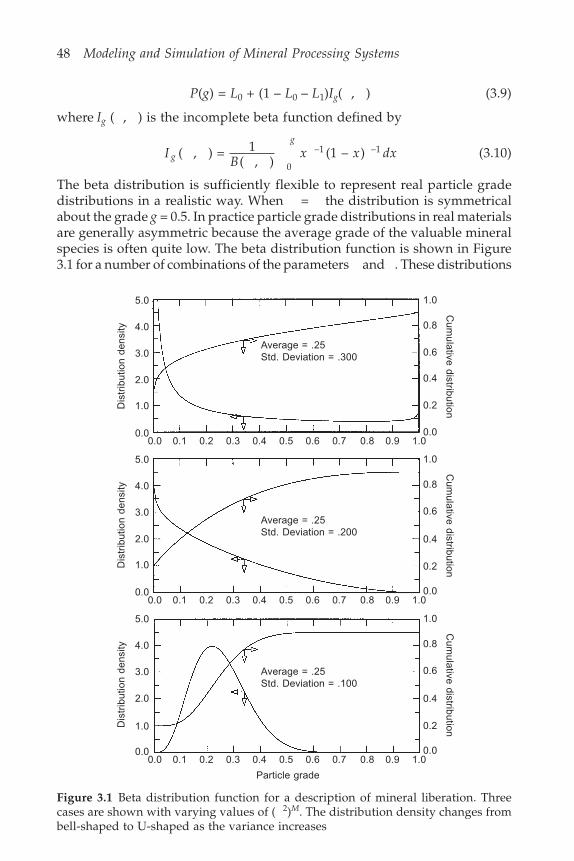
48 Modeling and Simulation of Mineral Processing Systems
P(g) = L0 + (1 – L0 – L1)Ig( , ) (3.9)
where Ig ( , ) is the incomplete beta function defined by
IB
x x dxg
g
( , ) = 1( , )
(1 – )0
–1 –1 (3.10)
The beta distribution is sufficiently flexible to represent real particle gradedistributions in a realistic way. When = the distribution is symmetricalabout the grade g = 0.5. In practice particle grade distributions in real materialsare generally asymmetric because the average grade of the valuable mineralspecies is often quite low. The beta distribution function is shown in Figure3.1 for a number of combinations of the parameters and . These distributions
Figure 3.1 Beta distribution function for a description of mineral liberation. Threecases are shown with varying values of ( 2)M. The distribution density changes frombell-shaped to U-shaped as the variance increases
5.0
4.0
3.0
2.0
0.0
1.0
1.0
0.8
0.6
0.4
0.2
0.0
Average = .25Std. Deviation = .300
Cum
ulative distributionDis
trib
utio
n de
nsity
0.0 0.1 0.2 0.3 0.4 0.5 0.6 0.7 0.8 0.9 1.0
5.0
4.0
3.0
2.0
0.0
1.0
1.0
0.8
0.6
0.4
0.2
0.0
Average = .25Std. Deviation = .200
Cum
ulative distributionDis
trib
utio
n de
nsity
0.0 0.1 0.2 0.3 0.4 0.5 0.6 0.7 0.8 0.9 1.0
5.0
4.0
3.0
2.0
0.0
1.0
1.0
0.8
0.6
0.4
0.2
0.0
Average = .25Std. Deviation = .100
Cum
ulative distributionDis
trib
utio
n de
nsity
0.0 0.1 0.2 0.3 0.4 0.5 0.6 0.7 0.8 0.9 1.0
Particle grade
Mineral liberation 49
are shown as both distribution densities and cumulative distributions. Onthe cumulative distribution, the liberated mineral at each end of the distributionrepresented by the vertical discontinuities at g = 0 and g = 1. Note how thedistribution density changes from bell-shaped to U-shaped as the variance ofthe inner distribution varies from 0.1 (lower graph) to 0.3 (upper graph). Thisis an essential requirement for the description of mineral liberation distributionsfor different particle sizes. When the particle size is distinctly larger than thesizes of the mineral grains within the ore, most particles in the populationexhibit a mineral grade close to the mean value for the ore as a whole and thedistribution is bell-shaped. On the other hand when the particle size is distinctlysmaller than the sizes of the mineral grains, the tendency for liberated andnearly liberated particles to appear is greatly enhanced and the beta distributionfunction reflects this tendency by exhibiting a strong U-shape. In the limit, asthe variance approaches its maximum value g gM M(1– ) , the beta distributioncan also describe a particle population that consists of completely liberatedparticles only. These properties of the beta distribution are exploited in thefollowing sections to develop models for the liberation process.
In practice it is common to represent the liberated material in terms of thefraction of the available mineral that is liberated:
�1 1 = gL(3.11)
�0 0 = (1 – )g L
3.2 Graphical representation of theliberation distribution
The distribution density function that is described in Section 3.1 is notparticularly useful for practical work. There is no convenient way ofrepresenting the liberated material at each end of the distribution density.This deficiency can be overcome by using either the cumulative distributionon which the liberated ends appear as vertical steps at each end of the graphor as a histogram that displays the distribution of particles in a finite numberof grade classes. The three distributions in Figure 3.1 are shown as histogramsin Figure 3.2.
Although the histogram gives a useful graphical representation of theliberation data, it cannot be used directly to make accurate estimates of theaverage grade of particles in the population. The usual formula
g g p gi i i = ( )=1
12
(3.12)
will often produce estimates that are significantly in error because of thedifficulty in assigning appropriate values to the representative grade gi ofeach grade class i. An alternative formula, which avoids this difficulty, isbased on the cumulative distribution
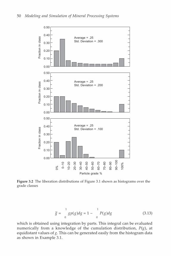
50 Modeling and Simulation of Mineral Processing Systems
g gp g dg P g dg = ( ) = 1 – ( )0
1
0
1
(3.13)
which is obtained using integration by parts. This integral can be evaluatednumerically from a knowledge of the cumulation distribution, P(g), atequidistant values of g. This can be generated easily from the histogram dataas shown in Example 3.1.
Figure 3.2 The liberation distributions of Figure 3.1 shown as histograms over thegrade classes
0.50
0.40
0.30
0.20
0.10
0.00
Average = .25Std. Deviation = .300
Fra
ctio
n in
cla
ss
0.50
0.40
0.30
0.20
0.10
0.00
Fra
ctio
n in
cla
ss
0.50
0.40
0.30
0.20
0.10
0.00
Fra
ctio
n in
cla
ss
0% 0–10
10–2
0
20–3
0
30–4
0
40–5
0
50–6
0
60–7
0
70–8
0
80–9
0
90–1
00
100%
Average = .25Std. Deviation = .200
Average = .25Std. Deviation = .100
Particle grade %

Mineral liberation 51
Illustrative example 3.1The histogram data for the distribution shown in the upper graph in Figure3.2 is given in Table 3.1. Use Equations 3.12 and 3.13 to make estimates of theaverage grade and compare these to the true average.
Table 3.1 Histogram data for the cumulative distribution shown in the top panel ofFigure 3.2
G-class Grade range p1(g) P (g) gi
1 0 0.2000 0.2000 0.002 0–10 0.3478 0.5478 0.053 10–20 0.0737 0.6215 0.154 20–30 0.0512 0.6727 0.255 30–40 0.0410 0.7137 0.356 40–50 0.0351 0.7488 0.457 50–60 0.0315 0.7803 0.558 60–70 0.0292 0.8095 0.659 70–80 0.0280 0.8375 0.75
10 80–90 0.0282 0.8657 0.8511 90–100 0.0343 0.9000 0.9512 100 0.1000 1.0000 1.00
g g p gi i i = ( ) = 0.285=1
12
The integral in Equation 3.13 can be conveniently evaluated using any equal-interval quadrature formula such as Simpson’s rule rather than the simpleEuler formula that is used in Equation 3.12. Using Simpson’s rule the averagegrade is calculated to be 0.281. These values can be compared to the correctvalue of (1 – 0.2 – 0.1)0.25 + 0.1 = 0.275. The error in calculating the averagehas been reduced from 3.8% to 2.2% using the more accurate formula. Thefractional liberation of the two minerals are
�1 = 0.275 0.1 = 0.0275
and
�0 = (1 – 0.275)0.2 = 0.145
3.3 Quantitative prediction of mineralliberation
Minerals are liberated from the host rock of an ore by grinding and in manymineral processing operations the sole purpose of any comminution operationis mineral liberation. Grinding operations are usually unselective in the sense

52 Modeling and Simulation of Mineral Processing Systems
that fractures that are induced in the rock show virtually no correlation withthe underlying mineralogical texture of the ore. There are exceptions to thisgeneral statement and some of the more important exceptions are examinedin some detail later in this chapter. The operations of crushing and grindingcan be regarded conceptually as the superimposition of a vast network offractures through the complex heterogeneous mineralogical texture of theore. The network of fractures ultimately determines the distribution of particlesizes that are produced in the comminution equipment. The relationshipbetween the network of fractures and the underlying mineralogical texturedetermines how the mineral phases are distributed among the particles inthe population after fracture. This concept can be observed in the particlesections that are shown in Figure 2.9 where the separate mineral phases aredisplayed at different gray levels so that they can be distinguished easily.
The purpose of any mathematical model of the liberation process is thecalculation of the liberation distribution that can be expected when mineralores are subjected to typical comminution operations. Quantitative modelsthat can be used for this purpose are not easy to develop and some specializedmethods must be used. Any model for liberation must begin with somequantitative description of the mineralogical texture of the ore. This is noeasy task because the ore texture is always complex in the geometrical sense.The most effective tool for the quantitative characterization of texture is imageanalysis. Samples of the ore are obtained and these are sectioned and polishedto reveal a plane section through the material. The section is examined usingoptical or electron microscopy and many digital images are collected torepresent the ore texture. These digital images are analyzed using specializedimage analysis software as described in Section 3.3.1. Typical sections throughtwo ores are shown in Figures 3.3 and 3.4.
3.3.1 Characterization of mineralogical texture byimage analysis
Because the texture of ores are so irregular in their geometrical constructionit is possible to characterize the texture only in terms of its statistical properties.This requires that many individual observations must be made and the relevantstatistical properties of the texture must be estimated from these observations.
The most useful properties to measure are those that will give some measureof the nature of the particles that are formed during grinding. Unfortunatelyit is not possible to know in advance how any particular piece of ore willfragment during the comminution operations and the fragmentation can onlybe simulated. The analysis that follows makes use of the concepts of theconditional distributions that are discussed in Section 2.7.
A simulation of the fracture pattern is obtained from a sample of actualparticles which have been mounted, sectioned, polished and imaged as shownfor example in Figure 3.5. The size and shape of these particles are characterizedby the distribution of linear intercepts which is determined by measuring thelength of very many intercept lengths across the particles as shown in Figures

Mineral liberation 53
Figure 3.3 Typical image of a section through mineral-bearing ore. Bright phase ispyrite, gray phases are silicates
Figure 3.4 Texture of coal. Bright phase is pyrite, gray phase is ash-forming mineralmatter and dark phase is the desired carbonaceous material
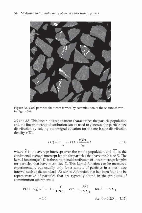
54 Modeling and Simulation of Mineral Processing Systems
2.9 and 3.5. This linear intercept pattern characterizes the particle populationand the linear intercept distribution can be used to generate the particle sizedistribution by solving the integral equation for the mesh size distributiondensity p(D):
P P D
p DdD
D
( ) = ( | ) ( )
0� � �
�(3.14)
where � is the average intercept over the whole population and �D is theconditional average intercept length for particles that have mesh size D. Thekernel function p(�|D) is the conditional distribution of linear intercept lengthsfor particles that have mesh size D. This kernel function can be measuredexperimentally but usually only for a sample of particles in a mesh sizeinterval such as the standard 2 series. A function that has been found to berepresentative of particles that are typically found in the products ofcomminution operations is
P D
DR
DDR
i ii( | ) = 1 – 1 –
1.2 exp –
1.2 for 1.2
–1
2
–1–1�
� ��
= 1.0 for � > 1.2Di–1 (3.15)
Figure 3.5 Coal particles that were formed by comminution of the texture shownin Figure 3.4

Mineral liberation 55
The conditioning variable DR indicates that this distribution applies to asample of particles in a mesh size interval having Di–1/Di = R rather than ata single size D.
When all particles are exactly of size D, R = 1 and
P D
D D( | ) = 1 – 1 –
1.2 exp –
1.2� � �
(3.16)
It is usual to use distributions that are weighted by length
f
p( ) =
( )�
� �
�(3.17)
and
f D
p D
D( | ) =
( | )�
� �
�(3.18)
and Equation 3.15 becomes
F F D p D dD( ) = ( | ) ( )
0� � (3.19)
which has the following useful kernel
F D
D( | ) = 1 – exp –
0.772�
�(3.20)
where the parameter is a function of the material and method of comminution.The distributions given in Equations 3.15 and 3.16 are parameter free and
can be used for many ores even when the linear intercept distribution for theparticles is not available. When the conditional linear intercept distributionof the particle population is known or can be estimated, the prediction of theexpected liberation characteristics of the ore can be calculated using thefollowing straightforward method.
The image of the unbroken ore is sampled by superimposing linear samplesdrawn from the population defined by Equation 3.14. Each linear sample willcover one or more of the phases and consequently can be characterized by itslinear grade gL which is the fraction of its length that covers the mineralphase. The sample lengths can be sorted into sizes and the distribution oflinear grades can be easily estimated for each different linear sample lengthwhich generates the conditional linear grade distribution P(gL| �) for the ore.This provides the necessary characterization of the ore texture from which itsliberation characteristics can be calculated.
The images that are used must be larger than the largest dimension of anytexture characteristic of the ore. This can be difficult to achieve if the sizescales of the different minerals in the ore are widely different. The pyriticquartzite and coal shown in Figures 3.3 and 3.4 are typical examples. Thepyritic quartzite includes large quartz pebbles which are completely barren
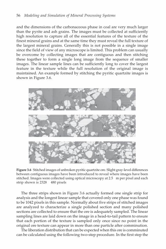
56 Modeling and Simulation of Mineral Processing Systems
and the dimensions of the carbonaceous phase in coal are very much largerthan the pyrite and ash grains. The images must be collected at sufficientlyhigh resolution to capture all of the essential features of the texture of thefinest mineral grains and at the same time they must reveal the full texture ofthe largest mineral grains. Generally this is not possible in a single imagesince the field of view of any microscope is limited. This problem can usuallybe overcome by collecting images that are contiguous and then stitchingthese together to form a single long image from the sequence of smallerimages. The linear sample lines can be sufficiently long to cover the largestfeature in the texture while the full resolution of the original image ismaintained. An example formed by stitching the pyritic quartzite images isshown in Figure 3.6.
Figure 3.6 Stitched images of unbroken pyritic quartzite ore. Slight gray-level differencesbetween contiguous images have been introduced to reveal where images have beenstitched. Images were collected using optical microscopy at 2.5 m per pixel and eachstrip shown is 2328 480 pixels
The three strips shown in Figure 3.6 actually formed one single strip foranalysis and the longest linear sample that covered only one phase was foundto be 1042 pixels in this sample. Normally about five strips of stitched imagesare analyzed to characterize a single polished section and many polishedsections are collected to ensure that the ore is adequately sampled. The linearsampling lines are laid down on the image in a head-to-tail pattern to ensurethat each portion of the texture is sampled only once since no point in theoriginal ore texture can appear in more than one particle after comminution.
The liberation distribution that can be expected when this ore is comminutedcan be calculated using the following two-step procedure. In the first step the

Mineral liberation 57
measured distribution of linear grades from the linear samples are combinedwith the linear intercept distribution density p(�|D) of the particles that areexpected to be formed during comminution of the ore. Equations 3.15, 3.16 or3.20 would be suitable models for the latter distribution. This produces thedistribution of linear grades in particles of size D from the equation
P g D P g p D dL L( | ) = ( | ) ( | )
0� � � (3.21)
This equation represents exactly the measurement of the linear gradedistribution by sampling particle sections from size D as described in Section2.7.2. The result of applying this transformation to the distribution of lineargrades measured on the texture shown in Figure 3.6 is given in Figure 3.7.
Equation 3.21 implies that P(gL|�, D) is independent of the particle size.This is valid provided that the fracture process is random and independentof the texture. The problem is considerably more complex when non-randomfracture patterns occur. Non-random fracture is discussed in Section 3.5.
Figure 3.7 Calculated distribution of linear intercepts as a function of particle sizefor texture shown in Figure 3.6
In the second stage of the calculation, the distribution of linear grades thatwas calculated using Equation 3.21 is transformed stereologically to generatethe distribution of grades in the real three-dimensional particles. This is identicalto the problem discussed in Section 2.7.3 for stereologically transformingmeasured linear grade distributions. The solution method is based ongenerating solutions to the integral equation
P g D P g g D p g D dgL L( | ) = ( | , ) ( | )0
(3.22)
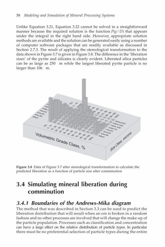
58 Modeling and Simulation of Mineral Processing Systems
Unlike Equation 3.21, Equation 3.22 cannot be solved in a straightforwardmanner because the required solution is the function P(g|D) that appearsunder the integral in the right hand side. However, appropriate solutionmethods are available and the solution can be generated easily using a numberof computer software packages that are readily available as discussed inSection 2.7.3. The result of applying the stereological transformation to thedata shown in Figure 3.7 is given in Figure 3.8. The difference in the ‘liberationsizes’ of the pyrite and silicates is clearly evident. Liberated silica particlescan be as large as 250 m while the largest liberated pyrite particle is nolarger than 106 m.
Figure 3.8 Data of Figure 3.7 after stereological transformation to calculate thepredicted liberation as a function of particle size after comminution
3.4 Simulating mineral liberation duringcomminution
3.4.1 Boundaries of the Andrews-Mika diagramThe method that was described in Section 3.3 can be used to predict theliberation distribution that will result when an ore is broken in a randomfashion and no other processes are involved that will change the make-up ofthe particle population. Processes such as classification and concentrationcan have a large effect on the relative distribution of particle types. In particularthere must be no preferential selection of particle types during the entire
Mineral liberation 59
comminution process. These conditions are normally not met in ball millcircuits which usually process feed that includes cyclone underflow and oftenother concentrates and tailing streams in addition to fresh feed. This complicatesthe calculation of the mineral liberation during comminution and it is necessaryto apply population balance techniques which can describe the fracture ofmulticomponent particles on a class-by-class basis. In this way the gradeclasses can be accurately accounted for among the breaking particles andevolution of the liberation distribution can be calculated at all stages in thecomminution process.
The effect of the mineral liberation phenomenon is described in thepopulation balance models through the breakage matrix b(x; x ) in Equation2.116. This matrix describes how particles transfer among the internalcoordinates during comminution. Two internal coordinates, particle size andparticle grade, are required to describe populations of multicomponentparticles. The matrix b(x; x ) is difficult to model in any particular case becauseit depends on both the liberation characteristics of the material, which aregoverned primarily by mineralogical texture, and also by the characteristicsof the comminution machine. In spite of the complexities, useful modelshave been developed and these have proved to be successful in simulationsof complex milling and concentration circuits. The approach that is used hereis based on a graphical representation of the breakage process called theAndrews-Mika diagram. These diagrams show what type of progeny particleswill be generated when a single parent particle breaks in a milling environment.The diagrams are useful because the graphical representation is fairly easy tointerpret and the diagrams explicitly include a number of essential constraintsthat must be applied to the breakage process in the population balance modelingmethod.
Particle size and particle grade must be included among the internalcoordinates to describe mineral liberation and the vector x of internalcoordinates is written for a two-component ore as
x = (g, dp) (3.23)
Here dp represents the particle size and g the particle grade. The breakagematrix b(x; x ) can be written as
b b g d g dp p( ; ) = ( , ; , )x x (3.24)
to reflect the two variables that make up the internal coordinates. This functioncan be simplified significantly using the rules of conditional distributionsdiscussed in Section 2.7
b g d g d b g d g d b d g dp p p p p p( , ; , ) = ( | ; , ) ( ; , ) (3.25)
To a large extent this decouples the breakage process from the liberationprocess and the two breakage functions can be modeled separately and thensubsequently combined using Equation 3.25 to generate the transformationfunction b g d g dp p( , ; , ) which is necessary to apply the population balance

60 Modeling and Simulation of Mineral Processing Systems
g g D d pu= [ / ]lib
method. The function b d g dp p( ; , ) can, in most cases, be assumed to beindependent of the grade g of the parent particle.
b d g d b d dp p p p( ; , ) = ( ; ) (3.26)
This is equivalent to asserting that the breakage function is independent ofthe grade of the parent particle. This appears to be a realistic assumption inmost practical cases. Models for the breakage function b d dp p( ; ) are discussedin Section 5.4. The function b g d g dp p( | ; , ) shows how the fracture productsof a parent particle of size dp and grade g are distributed with respect tograde for every possible progeny size. A useful practical model for this functionis developed in this section.
A geometric approach is taken and the nature of the function is describedby reference to the two-dimensional g – dp plane as shown in Figure 3.9. Anyparticle is located in this plane according to the values of its mineral grade gand its size dp. We wish to investigate how the progeny particles of a singleparent will dispose themselves in this two-dimensional phase space afterbreakage when the location of the parent particle is known. Of course thiscan be determined only in a probabilistic sense because the fracture processis random in character. Thus the liberation distributions for progeny particlesfrom a parent at point g dp, is required. To use the simplification that isinherent in Equation 3.25, the distributions that are conditional on the progeny
Figure 3.9 Boundaries of the Andrews-Mika diagram for the three cases: parent particlesize > liberation size, parent particle size liberation size, parent particle size <liberation size
1000
500
00.0 0.2 0.4 0.6 0.8 1.0 0.0 0.2 0.4 0.6 0.8 1.0 0.0 0.2 0.4 0.6 0.8 1.0
Par
ticle
siz
e
1000
500
0
1000
500
0
Parent particle
Liberation
size
BC
Attainable region R
g GF
Parent particle
Liberation
size
Attainable region R Attainable region R
A
A
A Parent particle
BC
G
Liberation
size
Fg GF
BC
Feeder region R
g
Particle grade Particle grade Particle grade
g g d dp p= [ / ]0.2
g g D d pu= [ / ]lib
d p
d p
d p
gd g dp p3 3 =

Mineral liberation 61
size, dp, are calculated. This gives the function b g d g dp p( | ; , ) which can becombined with the breakage function b d dp p( ; ) in Equation 3.26 for use inthe population balance Equation 2.116. A geometrical model is developedhere for b g d g dp p( | ; , ) in terms of a comparatively small number of parametersthat can be related to features of the mineralogical texture of the parentparticle.
Consider a parent particle at point A in Figure 3.9. When this particle isbroken, the progeny particles cannot appear at every point in the phasespace. They are restricted by definite physical constraints. Clearly progenycan appear only below point A because every progeny particle must be smallerthan the parent. In addition the progeny particles must satisfy the law ofconservation of phase volume. This means that no progeny particle can containa greater volume of mineral than the volume of mineral in the parent particle.Likewise no progeny particle can contain more gangue than was present inthe parent particle. These restrictions lead to the two inequalities
gv g vp p (3.27)
and
(1 – ) (1 – )g gp pv v (3.28)
where vp is the volume of the progeny particle and vp the volume of theparent particle. Since particles that are produced during comminutionare more or less geometrically similar, these inequalities can be writtenapproximately as
gd g dp p3 3 (3.29)
and
( 1 – ) (1 – )3 3g d g dp p (3.30)
These inequalities define two regions R and R in the phase space like thoseshown in the right hand panel of Figure 3.9. The diagrams shown in Figure3.9 are called Andrews-Mika diagrams in recognition of the first paper thatdescribed the boundaries and explored their significance.
The region R, called the attainable region, shows where progeny particlescan appear after fracture of a parent at point A. In particular the liberatededges of the region, represented by BF and CG in the diagram, are includedin the attainable region because an unliberated particle can generate completelyliberated particles. However, it is physically impossible for a parent at A togenerate any liberated particles larger than dpC or liberated gangue particleslarger than dpB. The region R is complementary to R and represents theregion of phase space that contains parent particles that could produce aprogeny at point A. This region is called the feeder region for progeny at A.Unlike the attainable region, the boundaries of the feeder region neitherintersect nor touch the vertical sides of the diagram at g = 0 and g = 1 because
62 Modeling and Simulation of Mineral Processing Systems
of the obvious fact that an unliberated progeny can never be produced froma liberated parent. The feeder region is important because it appears in thefundamental population balance Equation 2.110 for comminution machinesand it is necessary to establish the boundaries of R to define the region ofintegration in that equation. The shape of the boundaries of R and R varyconsiderably depending on the location of the parent particle in the phasespace.
When the parent particle is significantly smaller than the average ‘grainsize’ of the mineral in the ore, the parent will appear under the microscope asshown in image D of Figure 3.10. Under these conditions the parent willtypically contain only a single region of mineral and a single region of gangueand inequalities 3.29 and 3.30 are realistic bounds for the regions R and R .
This is not true when the parent particle is larger than the mineral ‘grainsize’. Two other cases can be distinguished: the parent size is comparable tothe mineral ‘grain size’ and the situation when the parent size is much largerthan the mineral ‘grain size’. These situations are illustrated in images B andC respectively in Figure 3.10, which are from the same material but weremade from particles of different size and magnification. The texture appearsto change from size to size but it is only the apparent texture that changes.The overall texture is of course the same. Textures that display this characteristicare called non-fractal to distinguish them from synthetic textures made usingfractal generators and which appear to be qualitatively similar no matterwhat scale and magnification is used to observe them. If the texture weretruly fractal, each apparently uniform mineral grain in Figure 3.10 wouldappear to be fragmented and made up of much smaller grains.
These geometrical properties of textures affect the boundaries of the feederand attainable regions. This can be seen most easily by considering point Cin the right hand panel of Figure 3.9 which is drawn at the intersection of theboundary of the attainable region and the line g = 1. This point reflects theprinciple that the largest completely liberated progeny particle cannot exceedthe total size of the mineral phase in the parent. If the parent particle containsonly a single mineral grain as is suggested, for example, by the lower imagein Figure 3.11, the largest grain is proportional to g dp
3 which is reflected ininequality 3.29. However, when the parent particle contains several separatemineral grains as shown in the upper diagram in Figure 3.11, the intersectionof the attainable region boundary with g = 1 must reflect the principle thatthe size of the largest liberated mineral particle in the progeny populationcannot exceed the size of the largest single coherent mineral grain in theparent particle. If there is more than one grain in the parent, the size of thelargest single grain must be smaller than g dp
3 and the upper boundary ofthe attainable region must fall below g dp
3 . This is illustrated in the left handand center panels of Figure 3.9. Similar arguments can be made for the ganguephase, which is reflected in the left hand boundaries of the attainable regionsshown in Figure 3.9. Boundaries for the feeder and attainable regions for thissituation can be defined by analogy to inequalities 3.29 and 3.30 as

Mineral liberation 63
gd g d
g d g d
p p
p p(1 – ) (1 – )(3.31)
with 3. The exponent varies with parent size and a model for thisvariation that has been found to be useful in practice is
Figure 3.10 Images that show the non-fractal nature of a typical mineralogical texture.A is a section through the unbroken ore. B is a section through a single particle fromthe 950–1180 m screen fraction at 20 magnification. C is from the 212–300 m screenfraction at 70 magnification. D is from the 53–75 m screen fraction at 300magnification
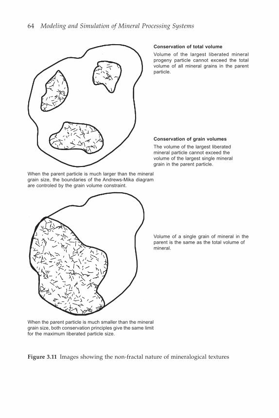
64 Modeling and Simulation of Mineral Processing Systems
Conservation of total volume
Volume of the largest liberated mineralprogeny particle cannot exceed the totalvolume of all mineral grains in the parentparticle.
Conservation of grain volumes
The volume of the largest liberatedmineral particle cannot exceed thevolume of the largest single mineralgrain in the parent particle.
When the parent particle is much larger than the mineralgrain size, the boundaries of the Andrews-Mika diagramare controled by the grain volume constraint.
Volume of a single grain of mineral in theparent is the same as the total volume ofmineral.
When the parent particle is much smaller than the mineralgrain size, both conservation principles give the same limitfor the maximum liberated particle size.
Figure 3.11 Images showing the non-fractal nature of mineralogical textures
Mineral liberation 65
= min , 30libD
dp
x
(3.32)
for d Dp lib where Dlib is a parameter referred to as the liberation size forthe ore. It is roughly equal to the particle size at which the mineral starts toliberate significantly when the ore is comminuted. x is a parameter which isapproximately 0.5. The upper limit of = 3 represents the law of conservationof phase volume and must never be exceeded.
The symmetry of the texture is also an important factor in fixing theboundaries of the attainable and feeder regions. A symmetrical texture is onein which the different mineral phases cannot be distinguished from geometricalfactors alone. The most common asymmetric texture is one in which distinctgrains of one mineral are imbedded in a more or less continuous phase ofanother mineral. To account for this effect the exponent can be different forthe mineral and the gangue. Thus inequalities 3.29 and 3.30 are written
gd g d
g d g d
p p
p p
u u
l l(1 – ) (1 – )(3.33)
The asymmetry factor for the texture is the ratio u/ l with u l = .When the parent size is much greater than the liberation size Dlib, and
when the progeny particles are also larger than Dlib, these will retain theparent composition or at most will be only slightly less or slightly greaterthan the parent composition. The attainable region is narrow for these progenyand useful approximations to the boundaries are shown in the left handpanel of Figure 3.9 and are given by
g gdd
gDdu
p
p p
u
max , 0.2
lib(3.34)
1 – max (1 – ) , (1 – )0.2
libg gdd
gDdl
p
p p
l
(3.35)
In spite of the empirical nature of these relationships, the parameters can beestimated reliably from batch comminution tests on two-component ores.
3.4.2 Internal structure of the Andrews-Mika diagramThe boundaries of the Andrews-Mika diagram are not sufficient to definehow progeny particles are distributed when a parent of given size and gradeis broken. The internal structure of the diagram contains this informationand a useful model for this internal structure is developed here which isbased on the beta distribution.
The model is based on the assumption that the progeny particle population
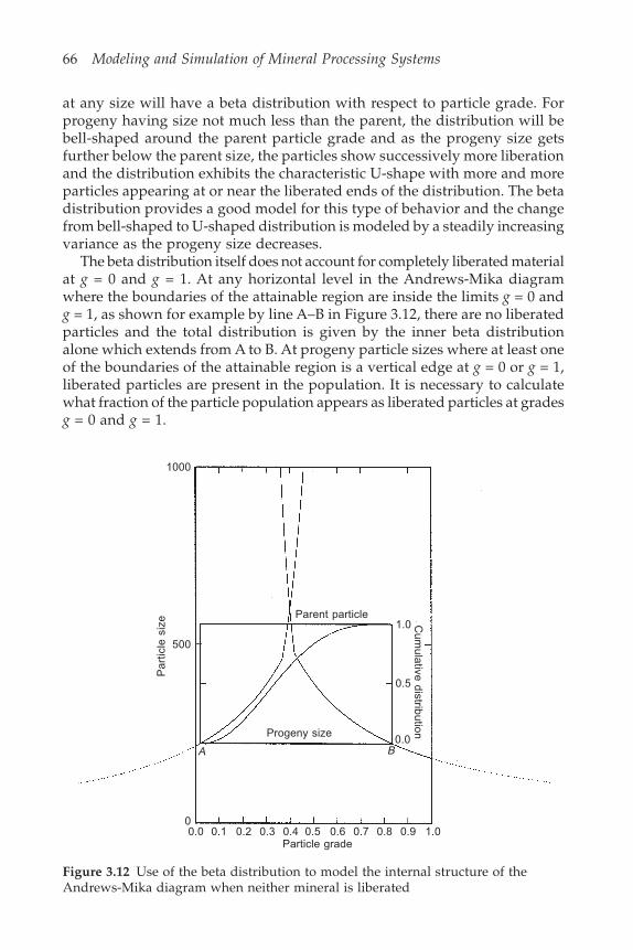
66 Modeling and Simulation of Mineral Processing Systems
at any size will have a beta distribution with respect to particle grade. Forprogeny having size not much less than the parent, the distribution will bebell-shaped around the parent particle grade and as the progeny size getsfurther below the parent size, the particles show successively more liberationand the distribution exhibits the characteristic U-shape with more and moreparticles appearing at or near the liberated ends of the distribution. The betadistribution provides a good model for this type of behavior and the changefrom bell-shaped to U-shaped distribution is modeled by a steadily increasingvariance as the progeny size decreases.
The beta distribution itself does not account for completely liberated materialat g = 0 and g = 1. At any horizontal level in the Andrews-Mika diagramwhere the boundaries of the attainable region are inside the limits g = 0 andg = 1, as shown for example by line A–B in Figure 3.12, there are no liberatedparticles and the total distribution is given by the inner beta distributionalone which extends from A to B. At progeny particle sizes where at least oneof the boundaries of the attainable region is a vertical edge at g = 0 or g = 1,liberated particles are present in the population. It is necessary to calculatewhat fraction of the particle population appears as liberated particles at gradesg = 0 and g = 1.
Figure 3.12 Use of the beta distribution to model the internal structure of theAndrews-Mika diagram when neither mineral is liberated
1000
500
0
A
0.0 0.1 0.2 0.3 0.4 0.5 0.6 0.7 0.8 0.9 1.0
B
Progeny size
Parent particle1.0
0.5
0.0
Cum
ulative distribution
Particle grade
Par
ticle
siz
e
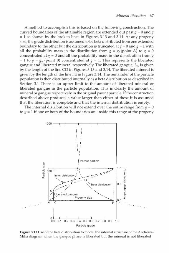
Mineral liberation 67
A method to accomplish this is based on the following construction. Thecurved boundaries of the attainable region are extended out past g = 0 and g= 1 as shown by the broken lines in Figures 3.13 and 3.14. At any progenysize, the grade distribution is assumed to be beta distributed from one extendedboundary to the other but the distribution is truncated at g = 0 and g = 1 withall the probability mass in the distribution from g = gl (point A) to g = 0concentrated at g = 0 and all the probability mass in the distribution from g= 1 to g = gu (point B) concentrated at g = 1. This represents the liberatedgangue and liberated mineral respectively. The liberated gangue, L0, is givenby the length of the line CD in Figures 3.13 and 3.14. The liberated mineral isgiven by the length of the line FE in Figure 3.14. The remainder of the particlepopulation is then distributed internally as a beta distribution as described inSection 3.1 There is an upper limit to the amount of liberated mineral orliberated gangue in the particle population. This is clearly the amount ofmineral or gangue respectively in the original parent particle. If the constructiondescribed above produces a value larger than either of these it is assumedthat the liberation is complete and that the internal distribution is empty.
The internal distribution will not extend over the entire range from g = 0to g = 1 if one or both of the boundaries are inside this range at the progeny
Figure 3.13 Use of the beta distribution to model the internal structure of the Andrews-Mika diagram when the gangue phase is liberated but the mineral is not liberated
1000
500Inner distribution
DLiberated gangue
Progeny size
0.0 0.1 0.2 0.3 0.4 0.5 0.6 0.7 0.8 0.9 1.0
Particle grade
1.0
0.5
0.0
Beta distribution
A C
0
B
Par
ticle
siz
e
Parent particle
Cum
ulative distribution
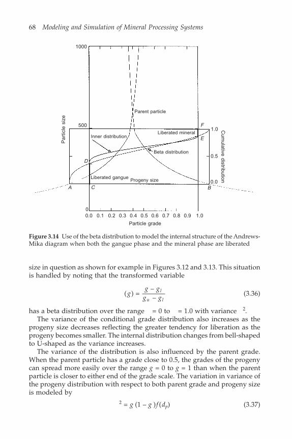
68 Modeling and Simulation of Mineral Processing Systems
size in question as shown for example in Figures 3.12 and 3.13. This situationis handled by noting that the transformed variable
( ) = ––
gg g
g gl
u l(3.36)
has a beta distribution over the range = 0 to = 1.0 with variance 2.The variance of the conditional grade distribution also increases as the
progeny size decreases reflecting the greater tendency for liberation as theprogeny becomes smaller. The internal distribution changes from bell-shapedto U-shaped as the variance increases.
The variance of the distribution is also influenced by the parent grade.When the parent particle has a grade close to 0.5, the grades of the progenycan spread more easily over the range g = 0 to g = 1 than when the parentparticle is closer to either end of the grade scale. The variation in variance ofthe progeny distribution with respect to both parent grade and progeny sizeis modeled by
2 = g (1 – g ) f (dp) (3.37)
1000
500
Par
ticle
siz
e
A C
D
Liberated gangue
Inner distribution
Beta distribution
Liberated mineral
Progeny size
Parent particle
F
E
B
1.0
0.5
0.0
Cum
ulative distribution
0.0 0.1 0.2 0.3 0.4 0.5 0.6 0.7 0.8 0.9 1.0
Particle grade
Figure 3.14 Use of the beta distribution to model the internal structure of the Andrews-Mika diagram when both the gangue phase and the mineral phase are liberated
0
Mineral liberation 69
with
f dd
D
pp
( ) = 1
1 + lib
(3.38)
The function f(dp) is S-shape in the range 0 to 1 as dp varies from large sizesto very small sizes. This function has the greatest variation when dp is closeto the mineral liberation size which reflects the tendency of the mineral toliberate over a comparatively narrow range of sizes. This phenomenon hasoften been observed in typical ore textures.
Substitution of Equation 3.37 into Equation 3.7 gives
= 1 – ( )
( )f d
f dp
p(3.39)
The parameters of the internal distribution must be chosen so that the averagegrade of the conditional distribution at every progeny size is equal to theparent grade:
g gp g d g d dgg L
L LM
g
g
p p
l
u
= ( | ; , ) = –
1 – –1
1 0(3.40)
The two parameters of the internal distribution are calculated from M = gM
and M = (1 – gM) . In fact, Equation 3.40 holds only if the fracture process israndom and no preferential breakage of one or other of the mineral phasesoccurs. Preferential breakage is discussed in Section 3.5.
3.5 Non-random fractureWhen the fracture pattern that is developed in the ore during comminutionis not independent of the mineralogical texture, the fracture process isconsidered to be non-random. Significant progress has been made onquantifying the effects of non-random fracture when particle fracture isinfluenced by the mineralogical composition and the texture of the parentparticle. Six separate non-random fracture effects have been identified whenmulti phase particles are broken:
1. Selective breakage. This occurs when the different mineral phases have unequalbrittleness. The more brittle mineral fractures more easily, and accordinglyparticles that have a larger content of the more brittle phase will have a largerspecific rate of breakage. This phenomenon does not influence the nature ofthe Andrews-Mika diagram directly and is described entirely through thebreakage rate parameters in the population balance equation. The parameterk in Equation 5.94 must be considered to be a function of both the particle sizeand the grade of the particle. This is discussed further in Section 5.8.3.
70 Modeling and Simulation of Mineral Processing Systems
2. Differential breakage. This occurs when the conventional breakage functiondepends on the composition of the parent particle. In other words, the sizedistribution of the progeny from a single breakage event will be influencedby the composition of the parent particle.
3. Preferential breakage. This occurs when crack branching occurs more frequentlyin one of the mineral phases. The most obvious manifestation of preferentialbreakage is a variation of average composition with particle size in the particlepopulations. This is often noticed in practice and is usually comparativelyeasy to detect and measure. Good models are available to incorporatepreferential fracture into the Andrews-Mika diagram and comparisons withexperimental observations have been satisfactory.
4. Phase-boundary fracture. This occurs when cracks have a significant tendencyto move along interphase boundaries rather than across the phases. Phase-boundary fracture destroys interphase boundary area in the progeny particles,and this should be measurable by careful image analysis. However, noconvincing evidence of significant phase-boundary fracture has been reportedin the literature.
5. Liberation by detachment. This occurs when mineral grains are comparativelyloosely bonded into the ore matrix. Mineral grains become detached from theore during comminution, which leads to significant and clean liberation ofthe mineral phases. This is unfortunately a fairly rare phenomenon and is notoften encountered with large ore bodies.
6. Boundary-region fracture. This occurs when the highly stressed region in theneighborhood of the boundary between two dissimilar minerals is preferentiallyfractured. This leads to the production of comparatively more smaller particlesfrom the phase-boundary region and therefore to less liberation among finerparticles than among coarser particles which originate preferentially fromthe interior of the mineral phases. Although there is some direct evidencethat boundary-region fracture does occur, this phenomenon is usually inferredfrom indirect observations on the behavior of the particles in concentrationplants. For example, preferential fracture in the neighborhood of a minormineral component will lead to a more than proportionate showing of thatmineral on the surfaces of the particles. This can have a profound effect onthe response of the particles to flotation. This is a complex phenomenon andno quantitative models have yet been developed to describe the effectconvincingly.
Only the first three of these six non-random fracture effects have beenmodeled successfully and the last three require considerably more research.Selective breakage can be simulated by determining the brittleness of eachmineral species and modeling the selection function in terms of the brittlenessratio as follows
Mineral liberation 71
k g dg g k d
pp
00
( , ) = 2( + (1 – ) ) ( )
1 + (3.41)
In Equation 3.41, k0(dp) is the specific rate of breakage as a function only of thesize of the parent particle. Models for k0(dp) are discussed in Section 5.12. Thebrittleness ratio can be measured using micro indentation techniques onpolished sections of the minerals.
When differential breakage occurs the approximation of Equation 3.26cannot be used and the size breakage function and a collection of breakagefunctions for each parent composition must be used. Such breakage functionscan be measured in the laboratory using single impact or slow compressiontesting devices.
If one of the mineral phases breaks preferentially it will end up in greaterconcentration in the finer sizes after comminution. Although it is not possibleto predict this phenomenon from a study of the mineralogy, it can be observedeasily in size-by-size assays of a simple laboratory batch mill test. This willreveal the systematic variation of mineral content with size. Preferentialbreakage has a strong influence on the internal structure of the Andrews-Mika diagram. Equation 3.40 can be relaxed and replaced with the requirementthat the average mineral grade over the total particle population must beconserved. Thus
0 0
1
( , | , ) = d
p p p
p
gb g d g d dgdd g (3.42)
for every combination of parent grade and size. Using Equation 3.25 thisrestriction becomes
0 0
1
( | , ) ( | ; , ) = d
p p p p p
p
b d g d gb g d g d dgdd g (3.43)
The preferential breakage is modeled by finding how the conditional mean
g d g d gb g d g d dgp p p p( ; , ) = ( | ; , )0
1
(3.44)
of the progeny particles varies with their size and parent composition. Amodel that has been found to satisfy data for several ores is
g d g dp g g g vddp
p
p( ; , ) = (1 – ) (3.45)
with
0( | , ) = 0
dp
p pp
ppb d g d v
dd
dd (3.46)
72 Modeling and Simulation of Mineral Processing Systems
Provided that the function v d dp p( / ) satisfies Equation 3.46, the conservationconstraint will be satisfied. The positive sign is used in Equation 3.45 whenthe mineral fractures preferentially and the negative sign is used when thegangue fractures preferentially.
A function which satisfies this requirement and which is suggested bytypical experimental data is
v(u) = u ln(u) (3.47)
with
= – 1ln( *)u
(3.48)
u
dd
p
p =
1 –
1 – 0(3.49)
This model for preferential breakage has two parameters. Values for theseparameters must be found from experimental data. 0 is a parameter that isadjusted to satisfy Equation 3.46. u* can be estimated directly from a plot ofmineral grade against particle size in the comminution product. Usually sucha plot shows a clear maximum or minimum. u* is the value of u at themaximum or minimum. The data shown in Figure 3.15 demonstrates this.
3.6 Discretized Andrews-Mika diagramThe models for the boundaries and internal structure of the Andrews-Mikadiagram that are developed in the preceding sections are based on thecontinuous beta distribution. They are not particularly useful for calculationsin this form and discrete versions are developed here for use in the discretizedpopulation balance models for ball mills that are described in Chapter 5. It iscommon practice to classify the grade variable into 12 or 22 classes over therange [0, 1]. Twelve classes allow one class at each end of the distribution forliberated mineral and for liberated gangue and 10 intervals in (0, 1). Theseare often of equal width but this is not essential. Twenty-two classes allow for20 internal classes which are usually 0.05 grade units in width. The conditionaldiscrete distribution can be obtained from the cumulative conditionaldistribution using the following equations
p g d g d P G d g d P G d g di i pj k pl i pj k pl i pj k pl( | ; , ) = ( | ; , ) – ( | ; , )+1(3.50)
= (1 – – ) ( , ) – ( , 0 1 ( ) ( )+1L L I IGM M
GM M
i i !Gi is the grade at the boundary between the i – 1 and i grade class.
A shorthand notation is used to describe the discrete versions of these

Mineral liberation 73
distribution functions.
a p g d g di jkl i i pj k pl, = ( | ; , ) (3.51)
The coefficients ai,jkl make up a discrete version of the attainable region of theAndrews-Mika diagram and examples are shown in Figures 3.16 and 3.17.Each bar in the attainable region shows what fraction of the parent particletransfers to each progeny class on breakage. The bar heights in the diagramare normalized so that the total height of all bars at a particular size is unity.This is consistent with the use of the conditional distributions in the continuousmodels described in Sections 3.4 and 3.5.
When this model for mineral liberation is inserted into the populationbalance equations for the ball mill, the feeder region for each point in thephase space rather than the attainable region from each parent location isrequired. The models developed in Sections 3.4 and 3.5 provide a logical andconsistent description of the attainable region and it would be much moredifficult to develop models for the feeder region. It is simpler to generate thefeeder region from the known structure of the attainable region. Let bi,jkl bethe fraction of size l to size j transfers that appear in grade class i when theparent is in grade class k. The relationship between the attainable and feederregions is
Figure 3.15 Data showing variation of grade with particle size when preferentialbreakage occurs
1.0
0.8
0.6
0.4
0.2
0.0
Ave
rage
gra
de
10–2 2 3 4 5 6 7 8 9 10–1 2 3 4 5 6 7 8 9100
Particle size, microns
Calculated from model with feed grade = 0.11Experimental data with feed grade = 0.11Calculated from model with feed grade = 0.41Experimental data with feed grade = 0.41Calculated from model with feed grade = 0.47Experimental data with feed grade = 0.47Experimental data with feed grade = 0.71Experimental data with feed grade = 0.83Calculated from model with feed grade = 0.71Calculated from model with feed grade = 0.83
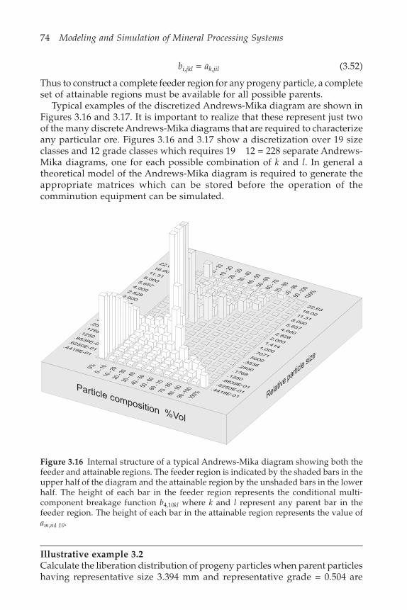
74 Modeling and Simulation of Mineral Processing Systems
bi,jkl = ak,jil (3.52)
Thus to construct a complete feeder region for any progeny particle, a completeset of attainable regions must be available for all possible parents.
Typical examples of the discretized Andrews-Mika diagram are shown inFigures 3.16 and 3.17. It is important to realize that these represent just twoof the many discrete Andrews-Mika diagrams that are required to characterizeany particular ore. Figures 3.16 and 3.17 show a discretization over 19 sizeclasses and 12 grade classes which requires 19 12 = 228 separate Andrews-Mika diagrams, one for each possible combination of k and l. In general atheoretical model of the Andrews-Mika diagram is required to generate theappropriate matrices which can be stored before the operation of thecomminution equipment can be simulated.
Figure 3.16 Internal structure of a typical Andrews-Mika diagram showing both thefeeder and attainable regions. The feeder region is indicated by the shaded bars in theupper half of the diagram and the attainable region by the unshaded bars in the lowerhalf. The height of each bar in the feeder region represents the conditional multi-component breakage function b4,10kl where k and l represent any parent bar in thefeeder region. The height of each bar in the attainable region represents the value ofam,n4 10.
Illustrative example 3.2Calculate the liberation distribution of progeny particles when parent particleshaving representative size 3.394 mm and representative grade = 0.504 are

Mineral liberation 75
broken by random fracture. Assume that the texture is symmetrical and thatthe liberation size parameter for the ore is 200 m. Consider two cases: progenysize is 212 m which is close to the liberation size, and progeny size = 53 mwhich is considerably smaller than the liberation size.
Values for other parameters in the model are 0 = 2.0, x = 0.5, asymmetryfactor = 1.0 and = 1.0.
Case 1: Progeny size = 212 mCalculate the boundaries of the Andrews-Mika diagram.
= min 2.02003394
, 3 = 0.2430.5
Texture is symmetrical, so � = u = = 0.243The upper boundary is calculated using Equation 3.34
gu = max 0.5043394212
, 0.504200212
0.2 0.243
Figure 3.17 Internal structure of a typical Andrews-Mika diagram showing both thefeeder and attainable regions. The feeder region is indicated by the shaded bars in theupper half of the diagram and the attainable region by the unshaded bars in the lowerhalf. The height of each bar in the feeder region represents the conditional multi-component breakage function b7,10kl where k and l represent any parent bar in thefeeder region. The height of each bar in the attainable region represents the value ofam,n7 10.

76 Modeling and Simulation of Mineral Processing Systems
= max [0.878, 0.497]
= 0.878
The lower boundary is calculated using Equation 3.35
1 – = max 0.496 3394212
, 0.496200212
0.2 0.243
g�
= max [0.864, 0.489]
g� = 0.136
Both boundaries lie within the range g = 0 to g = 1, so that the variable
=
––
g gg gu
�
� has a Beta distribution. Thus the cumulative conditional
distribution for progeny particles of size 212 m is
P(g|212; 0.504, 3394) = 0.0 for g g�
= Ix(g)( , ) for g� < g < gu
= 1.0 for g ∀ gu
The parameters and in this distribution are calculated from
#= (g)
= 0.504 – 0.1360.878 – 0.136
= 0.496
#####= (1 – (g ))
= 0.504#
The parameter determines the variance of the distribution
f dp( ) = 1
1 + 212200
= 0.4851.0
= 1 – ( )
( ) = 1 – 0.485
0.485 = 1.061
f df d
p
p
= 0.496 1.061 = 0.526
= 0.504 1.061 = 0.585
Since both and are less than 1, the distribution is U-shaped, which indicatesthat the minerals are rapidly approaching liberation as the progeny size passesthe mineral grain size.
The cumulative distribution and the corresponding histogram is shown inFigure 3.18

Mineral liberation 77
Case 2: Progeny size = 53 mIn this case, the boundaries fall outside the range g = 0 to g = 1 and
completely liberated particles will be found in the progeny population.
gu = max 0.5013394
53, 0.504
20053
0.2 0.243
= max [1.158, 0.696]
= 1.158
1 – = max 0.4963394
53, 0.496
20053
0.2 0.243
g�
= max [1.140, 0.685]
= 1.140
g� = – 0.140
The liberated factions are calculated from the Beta distribution of thetransformed variable,
( ) = + 0.140
1.158 + 0.140g
g
which has parameters
f dp( ) = 1
1 + 53200
= 0.791
= 1 – 0.7910.791
= 0.265
1.0
0.8
0.6
0.4
0.2
0.00.0 0.2 0.4 0.6 0.8 1.0
Particle grade
Cum
ulat
ive
dist
ribut
ion
0.50
0.40
0.30
0.20
0.10
0.00
Fra
ctio
n in
cla
ss
0% 0–10
10–2
020
–30
30–4
040
–50
50–6
060
–70
70–8
080
–90
90–1
0010
0%
Particle grade %
Figure 3.18 Cumulative distribution and histogram of particle grades at progeny sizeof 212 m.
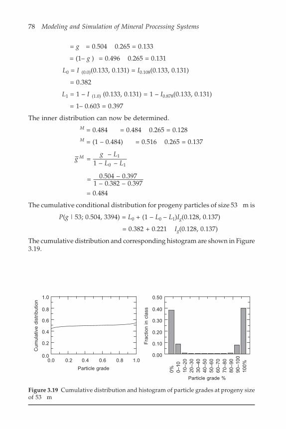
78 Modeling and Simulation of Mineral Processing Systems
= g = 0.504 0.265 = 0.133
= (1– g ) = 0.496 0.265 = 0.131
L0 = I (0.0)(0.133, 0.131) = I0.108(0.133, 0.131)
= 0.382
L1 = 1 – I (1.0) (0.133, 0.131) = 1 – I0.878(0.133, 0.131)
= 1– 0.603 = 0.397
The inner distribution can now be determined.M = 0.484 = 0.484 0.265 = 0.128M = (1 – 0.484) = 0.516 0.265 = 0.137
gg L
L LM =
–1 – –
1
0 1
= 0.504 – 0.3971 – 0.382 – 0.397
= 0.484
The cumulative conditional distribution for progeny particles of size 53 m is
P(g | 53; 0.504, 3394) = L0 + (1 – L0 – L1)Ig(0.128, 0.137)
= 0.382 + 0.221 Ig(0.128, 0.137)
The cumulative distribution and corresponding histogram are shown in Figure3.19.
Figure 3.19 Cumulative distribution and histogram of particle grades at progeny sizeof 53 m
1.0
0.8
0.6
0.4
0.2
0.00.0 0.2 0.4 0.6 0.8 1.0
Particle grade
Cum
ulat
ive
dist
ribut
ion
0.50
0.40
0.30
0.20
0.10
0.00
Fra
ctio
n in
cla
ss
0% 0–10
10–2
020
–30
30–4
040
–50
50–6
060
–70
70–8
080
–90
90–1
0010
0%
Particle grade %
Mineral liberation 79
3.7 Symbols used in this chapterB( , ) Beta function.b d dp p( : ) Breakage function.b g d g dp p( , : , ) Breakage function for 2-component material.dp Particle size.D Mesh size.f (�) Distribution density (by length) for intercept length.f (dp) Variation of variance with progeny size.g Mineral grade of particle.gL Linear grade.Ig Incomplete beta function.
� Average intercept length.
�D Average intercept length for particles of size D.L0 Mass fraction of particle population that consists of
liberated gangue.L1 Mass fraction of particle population that consists of
liberated mineral.�0 Fraction of available gangue that is liberated.�1 Fraction of available mineral that is liberated.p(D) Distribution density for particle size.p(g) Distribution density for particle grade.p(�) Distribution density for intercept length.p(�|D) Conditional density for intercept length from particles
of size D.p(gL|�) Conditional density for linear grades in intercepts of
length �.DR Conditioning variable to indicate particles come from a
size interval.
BibliographyThe importance of mineral liberation and its description in terms of thegeometry of the mineralogical texture and the geometrical properties of theparticles was analyzed by Gaudin (1939) using simple geometrical structures.Barbery (1991) gave an account of most of the more recent research up to1990. Fander (1985) gives a well illustrated account of many mineral texturesas seen under the microscope. Jones (1987) provides an excellent account ofquantitative methods that are available for the analysis of mineralogical texture.King (1994) has presented an alternative theoretical method for the predictionof mineral liberation from measurements on sections which can be appliedwhen fracture is not random. Andrews and Mika (1976) analyzed the inter-relationship between comminution and liberation using population balancetechniques and this forms the basis of the modeling method discussed in thischapter. King (1990) provided a simple model for the internal structure of the
80 Modeling and Simulation of Mineral Processing Systems
Andrews-Mika diagram and Schneider (1995) developed the model to thestage where it could be calibrated using image analysis data obtained fromsamples of ore.
ReferencesAndrews, J.R.G. and Mika, T.S. (1976) Comminution of heterogeneous material.
Development of a model for liberation phenomena. Proc. 11th Int Mineral ProcessingCongress, pp. 59–88.
Barbery, G. (1991) Mineral Liberation. Measurement, Simulation and Practical Use in MineralProcessing. Editions GB, Quebec.
Fander, H.W. (1985) Mineralogy for Metallurgists: an Illustrated Guide. The Institution ofMining and Metallurgy, London.
Gaudin, A.M. (1939) Principles of Mineral Dressing. McGraw-Hill, New York.Jones, M.P. (1987) Applied Mineralogy: A Quantitative Approach. Graham and Trotman,
London.King, R.P. (1990) Calculation of the liberation spectrum in products produced in
continuous milling circuits. Proc. 7th European Symposium on Comminution, Vol. 2,pp. 429–444.
King, R.P. (1994) Linear stochastic models for mineral liberation. Powder Technology.Vol. 81, pp. 217–234.
Schneider, C.L. (1995) The Measurement and Calculation of Liberation in ContinuousGrinding Circuits. Ph.D Thesis, University of Utah.
4Size classification
It is always necessary to control the size characteristics of particulate materialthat is fed to process equipment that separates the mineralogical components.It is not possible within the production environment to exercise precise controlover the size of all particles in a population and, in most cases, size classificationequipment is designed to split a feed of particulate material into a coarse anda fine product. Occasionally one or two product streams of intermediate sizemay be produced such as by a double or triple deck screen. Probably themost common application of size classification is its use to prevent oversizematerial leaving a comminution circuit. Oversize material is recycled to acomminution stage for further size reduction before passing to subsequentstages of processing.
The most significant consideration when evaluating classification equipmentis the lack of a clean cut at a particular size. Even the most efficient industrialsize classifiers will pass a proportion of oversize material and will retain aportion of undersize material.
Size classification equipment is also subject to capacity limitations andthese must be considered when evaluating the performance of new or existingclassification equipment. In fact older methods of performance evaluationconcentrate entirely on the capacity limitations. However, more modernprocedures recognize that the efficiency of separation must also be consideredif the performance of a size classifier in a plant circuit is to be accuratelyevaluated. The procedures that follow take this into account.
There are essentially two types of classifier available for process operation:screens and classifiers that rely on the variation of terminal settling velocitiesof particles of varying size when these are immersed in a viscous fluid. Ingeneral the former are used for the classification of drier material at coarser sizes.
4.1 Classification based on sieving–vibratingscreens
The basic method of operation of a screen is simple. The screen presents abarrier to the passage of oversize material while it readily passes undersizematerial. It is only necessary to ensure that each particle has an opportunityto reach the screen. In practice each particle is given several opportunities topass through the screen. Screens can be stationary or the screen can vibratewhich increases the rate of presentation of each particle and assists in movingoversize material over and away from the screening surface.
82 Modeling and Simulation of Mineral Processing Systems
4.1.1 Models based on screen capacityThe traditional method of evaluation of screen performance is the use of acapacity measure. This represents the ability of the screen to accept andhandle the feed tonnage of material. The most important assumption in thisapproach is that the capacity of a screen is directly proportional to its surfacearea so that the basic capacity is specified at tons of feed per hour per squaremeter of screen. This quantity is represented by Iu. The basic capacity of anyscreen is determined under standard operating conditions using a predefinedstandard feed material. As the nature of the feed material changes and as theoperating conditions change so the actual capacity of the screen changes, itwill increase for conditions less arduous than the standard and decrease forconditions more arduous than the standard. These modifications are representedby capacity factors which multiply the standard unit screen capacity to getthe actual screen capacity under conditions that the screen will actually meetin its position in the operating plant
Rated screen feed capacity = IuK1K2 . . .
= Iu iKi tons/hr m2 (4.1)
where the separate Ki are the capacity factors for deviations from the standardconditions with respect to a number of individual conditions.
The basic unit capacity varies primarily with the size of the screen opening,screens with larger openings being able to handle large quantities of feedmaterial. A typical relationship between Iu and mesh size is:
Iu = 0.783h + 37 for h 25 mm (4.2)
= 20.0h0.33 – 1.28 for h < 25 mm (4.3)
where Iu is in tons/hr m2 and h is the mesh size in mms. Each screenmanufacturer has its own basic capacity-size relationships for its range ofscreens. The above expressions are only meant to define a typical trend.
The individual capacity factors are provided by screen manufacturers intabular or graphical form although the availability of computers is encouragingthe presentation of these factors in algebraic form. The following factors aretypical for woven wire mesh screens.
The open area factor K1The standard condition is usually 50% open area and the capacity is proportionalto the open area available.
K1 = % open area
50(4.4)
For material having a bulk density less than 800 kg/m3 the standard openarea is 60% rather than 50% and Equation 4.4 should be modified accordingly.
Size classification 83
The half-size factor K2Feed that contains a large proportion of material that is considerably smallerthan the screen mesh size will be handled more easily by a screen. The standardcondition is defined as feed material having 40% smaller than one half of themesh size. If the feed has more than 40% smaller than one half of the screenmesh size, the half-size factor will exceed unity and vice versa.
K2 = 2PF(0.5h) + 0.2 (4.5)
The oversize factor K3A screen can handle a greater tonnage of feed material that contains largequantities of oversize material because this material passes directly over thescreen and need not be transmitted through the mesh. This is accounted forby the oversize factor K3, which has a value of unity for a standard feedcontaining 25% oversize material. This factor increases very quickly as thefraction of oversize increases and is given by
K3 = 0.914 exp exp (4.22 ( ) – 3.50)P hF (4.6)
In Equation 4.6, P hF ( ) is the fraction of material in the feed that has sizegreater than the screen mesh size h. It is related to the cumulative sizedistribution function by
P hF( ) = 1 – PF(h) (4.7)
The bulk density factor K4Denser materials will be transmitted more easily than lighter materials. Afactor K4 accounts for this effect when bulk density differs from the standardof 1600 kg/m3.
K B4 =
1600(4.8)
The deck position factor K5Screens that are lower down in the deck receive undersize from the screenabove and can handle less material than a screen that takes fresh feed. Thecapacity decreases with position according to capacity factor K5.
K5 = 1.1 – 0.1S (4.9)
where S represents the deck position; 1 for top deck, 2 for 2nd deck and so on.
The screen angle factor K6The standard inclined screen has an angle of inclination of 15 . Lower anglesof inclination increase the projected area of the screen aperture in the horizontalplane and the screen can handle a greater load. This is accounted for bycapacity factor K6.

84 Modeling and Simulation of Mineral Processing Systems
K6 = 1.0 – 0.01( – 15) (4.10)
where is the angle of inclination in degrees.
The wet screen factor K7Screening at finer mesh sizes can be improved by spraying the screen loadwith water. The factor K7 accounts for this effect
K7 = 1.0 + 2.4 10–4(25 – h)2.5 for h 25 mm
= 1.0 for h > 25 mm (4.11)
The aperture shape factor K8The standard screen has square openings and other shapes influence thecapacity as shown in Table 4.1.
Table 4.1 Screen capacity factor for different apertures
Shape of screen opening K8
Round 0.8Square 1.02 to 1 rectangular slot 1.153 to 1 rectangular slot 1.24 to 1 rectangular slot 1.25
Particle shape factor K9Slabby and elongated particles are more difficult to screen than particles thatare essentially isometric. If the feed contains about 15% of slabby or elongatedparticles K9 should be set at 0.9. Larger amounts of this type of materialwould give significant problems and would need to be investigated specially.
The surface moisture factor K10Surface moisture tends to make the particles adhere and screen capacity isreduced. Factor K10 accounts for this and can be evaluated from Table 4.2.
Table 4.2 Surface moisture capacity factor for screens
Condition of feed K10
Wet, muddy or sticky material 0.75Wet surface quarried and material from 0.85surface stockpiles with up to 15% moisture by volumeDry crushed material 1.0Naturally or artificially dried material 1.25
Size classification 85
4.1.2 Screen transmission efficiencyIdeally the screen should be able to transmit all of the undersize material inthe feed. In practice, however, not all of the undersize material passes throughthe screen and the fraction of the feed undersize that does pass through isreferred to as the screen efficiency. The efficiency is determined primarily bythe actual feed loading on the screen relative to the rated feed capacity ascalculated by Equation 4.1. The efficiency of transmission decreases if thescreen must handle feed in excess of 80% of the rated tonnage because theaccess of individual particles to the screen surface is hindered to a greater orlesser degree. The efficiency also decreases as the actual feed tonnage fallsbelow 80% of rated capacity because particles tend to bounce on the lightlyloaded screen and make fewer contacts with the screen surface.
If WF represents the actual feed tonnage, then the rating ratio is given by:
RR WI K
F
u i i =
screen area(4.12)
and the efficiency of transmission is given by
e RR RR RR
RR RR
= 0.95 – 0.25( – 0.8) – 0.05( – 0.8) for 0.8= 0.95 – 1.67(0.8 – ) for < 0.8
2
2(4.13)
The actual tonnage passed to the undersize stream is
WU = ePF(h)WF (4.14)
Each size class smaller than the mesh size is subject to the same efficiencyfactor e so that the particle size distribution in the underflow stream is calculatedin discrete form as
pep W
eP h W
p
P hd h
d h
iU i
F F
F FiF
F pi
pi
= ( )
= ( )
for <
= 0 for
(4.15)
where piU is the fraction of the underflow stream in the size class i and
piF that fraction in the feed stream.The actual tonnage passed to the overflow stream is:
W P h W e P h W
W eP h
O F F F F
F F
= (1 – ( )) + (1 – ) ( )
= (1 – ( ))(4.16)
and the discrete size distribution in the overflow stream is given by:
pe p
eP hd hi
O iF
F p = (1 – )
(1 – ( )) for < (4.17)
=1 – ( )
for p
eP hd hi
F
F p (4.18)
86 Modeling and Simulation of Mineral Processing Systems
The simple capacity model permits the calculation of the total screen areathat is required for a specific duty. The aspect ratio of the screen (length/width ratio) must be determined by considering the depth of the bed ofparticles on the screen. An approximate guide is the restriction of the beddepth at the discharge end to no more than four times the mesh size. Thethickness of the bed is determined by the total flowrate over the screen surface,the width of the screen, b, and the velocity of travel of the material along thescreen.
t Wbub
O
B = (4.19)
where tb is the bed thickness, Wd the mass flowrate across the discharge end,b the screen width, u the velocity of travel across the screen surface and B thebulk density. The velocity of travel depends primarily on the angle of inclinationand the amplitude and mode of vibration.
4.2 The classification functionA more realistic description of the performance of a classification device isprovided by the classification function. This function defines the probabilitythat an individual particle will enter the oversize stream that leaves the classifier.This function is also known as the partition function, and, when showngraphically, as the partition curve. It is a complicated function of the particleproperties and the classifying action of the particular device underconsideration. The classification function c(dpi) is defined as the mass fractionof material in size interval i in the feed which finally leaves in the oversizestream.
Once the partition function is known, the size distribution in both overflowand underflow can be calculated by a simple mass balance over the solids insize class i.
W p c d W pUiU
piF
iF = (1 – ( )) (4.20)
W p c d W pOiO
piF
iF = ( ) (4.21)
where the superscripts O, U and F refer to oversize, undersize and feedrespectively.
The total flowrates of solid in the oversize and the undersize are given by:
W W p c d W pUi
UiU
i piF
iF = = (1 – ( )) (4.22)
W W p c d W pOi
OiO
i piF
iF = = ( ) (4.23)
p c d WW
pc d p
c d piU
piF
U iF pi i
F
i pi iF
= [1 – ( )] = [1 – ( )]
[1 – ( )](4.24)

Size classification 87
p c d WW
pc d p
c d piO
piF
O iF pi i
F
i pi iF
= ( ) = ( )
( )(4.25)
These formulas are often written in terms of the total yield of solids to theoverflow:
Y WW
sO
F = (4.26)
pc d p
YiU pi i
F
s =
(1 – ( ))1 –
(4.27)
pc d p
YiO pi i
F
s =
( )(4.28)
Y c d ps i pi iF = ( ) (4.29)
4.2.1 The Karra modelThe approach described in the previous section is the traditional methodused for sizing screens. Its chief limitation is that the screen must be sizedaccording to the amount of feed that is presented to the screen. A morelogical approach is based on the amount of material that must be actuallytransmitted by the screen to the underflow stream. This approach has beendeveloped by V.K. Karra (1979) into an effective description of how a screenmay be expected to perform during plant operation.
The approach is similar to the traditional approach but is based on thecapacity of the screen to transmit undersize material proportional to thescreen area. As in the traditional method this basic capacity is modified by anumber of factors that allow for variations of the feed material and the screenfrom the standard test conditions.
Let A represent the basic capacity which is defined as the tonnage ofundersize that a particular screen can transmit per unit of screen surface area.The basic capacity is increased or decreased depending on the nature of thefeed and conditions on the screen. A number of capacity factors allow for theamount of oversize in the feed (factor B), the amount of half size in the feed(factor C), the location of the deck (factor D), factor for wet screening (factorE) and for material bulk density (factor F). These factors all have a value ofunity at the nominal standard operating condition and move down or up asthe screening duty becomes more or less arduous. The amount of near-sizematerial also has a significant effect on the ability of the screen to transmitundersize material and an additional near-size capacity factor Gc is introduced.
The theoretical amount of undersize that can be transmitted by the screenis given by:
Th = A.B.C.D.E.F.Gc screen area (4.30)
88 Modeling and Simulation of Mineral Processing Systems
A screen will be well designed to handle its duty in the circuit if Th isapproximately equal to the quantity of undersize in the feed. Each of thecapacity factors is related to the quality of the feed and to the type of screen.
Karra bases the screen performance on the effective throughfall apertureof the screen defined by
hT = (h + dw) cos – dw (4.31)
where dw is the diameter of the wire and is the angle of inclination of thedeck. Equation 4.31 gives the effective aperture area projected onto thehorizontal plane which is appropriate for particles that must pass throughthe screen under gravity.
The basic capacity AThe basic capacity is primarily determined by the mesh size of the screenwith the effective throughfall aperture being used as the appropriate measureof screen mesh size.
A h hT T = 12.13 – 10.3 for < 51 mm0.32 (4.32)
A = 0.34 hT + 14.41 for hT 51 mm (4.33)
with hT in mm and A is in metric tons/hr m2.The basic capacity will also depend on the open area of the screen used.
The basic capacity calculated from Equations 4.32 and 4.33 is applicable tostandard industrial light-medium woven wire mesh. For other screen clothsand surfaces, A must be adjusted in proportion to the open area. The percentopen area for light-medium wire mesh is related to the mesh size h by
OA = 21.5 log10h + 37 (4.34)
with h in millimeters.Thus capacity A must be adjusted to:
AOA
actual % open area(4.35)
The oversize factor B
B P h P hB P h P h
FT
FT
FT
FT
= 1.6 – 1.2 ( ) for ( ) 0.87 = 4.275 – 4.25 ( ) for ( ) 0.87
(4.36)
The half-size factor C
C P h P hC P h P hC P h P hC P h P h
FT
FT
FT
FT
FT
FT
FT
FT
= 0.7 + 1.2 (0.5 ) for (0.5 ) 0.3 = 2.053 (0.5 ) for 0.3 < (0.5 ) 0.55 = 3.35 (0.5 ) for 0.55 < (0.5 ) 0.8 = 5.0 (0.5 ) – 1.5 for (0.5 ) 0.8
0.564
1.37(4.37)
Size classification 89
The deck location factor DD = 1.1 – 0.1S (4.38)
where S = 1 for top deck, S = 2 for 2nd deck and so on.
The wet screening factor ELet T = 1.26hT (hT in mm)
E = 1.0 for T < 1E = T for 1 T < 2E = 1.5 + 0.25T for 2 T < 4E = 2.5 for 4 T < 6E = 3.25 – 0.125T for 6 T < 10E = 4.5 – 0.25T for 10 T < 12E = 2.1 – 0.05T for 12 T < 16E = 1.5 – 0.0125T for 16 T < 24E = 1.35 – 0.00625T for 24 T < 32E = 1.15 for T > 32
whenever the material is sprayed with water.
The bulk density factor F
F B = 1600
(4.39)
The near-size capacity factor GcThe capacity of the screen is also affected by the presence of near-size materialin the feed. The near-size material in the feed is in the size range from 0.75hTto 1.25hT. Considerable quantities of near-size material will inhibit the passageof undersize material through the screen. The near-size capacity factor can beevaluated from:
G
G P h P hc
cF
TF
T
= 0.975(1 – near-size fraction in feed) = 0.975(1 – (1.25 ) + (0.75 )
0.511
0.511 (4.40)
4.2.2 The screen classification functionIn practice, not all of the undersize is transmitted because of various physicalfactors that impair the efficiency of the screen. This effect is described by thescreen partition function. Several standard functional forms are available todescribe this effect, and the Rosin-Rammler function is used here.
c(dp) = 1 – exp[– 0.693(dp/d50)5.9] (4.41)
This gives the efficiency of transfer of particles of size dp to oversize.The parameter that will determine the screening efficiency is d50. Values of
d50 greater than the mesh size give high efficiencies and vice-versa.The actual d50 achieved will depend primarily on the effective throughfall
90 Modeling and Simulation of Mineral Processing Systems
aperture of the wire mesh used on the screen, on a loading coefficient Kdefined by:
KABCDEF
W P hABCDEF
FT
= tons of undersize in the feed/unit of screen area
=( )/screen area (4.42)
and on the near-size factor Gc.Experimental screening data are well represented by:
dh
GKT
c500.148 = (4.43)
d50 can be substituted in Equations 4.41 and 4.20–25 to calculate the sizedistributions in the two product streams.
pc d p
c d piU pi i
F
i pi iF
= [1 – ( )]
[1 – ( )](4.44)
pc d p
c d piO pi i
F
i pi iF
= ( )
( )(4.45)
The model provides a simulation of the actual performance of the screen inthe circuit. This performance can be compared with the design capacity ofthe screen and the screen performance evaluated. In particular, the actualoperating efficiency can be calculated from
simulated efficiency = tonnage transmitted to undersize
tonnage of undersize in feed(4.46)
= [1 – ( )]
( )i pi i
F
F
c d p
P h(4.47)
The effective utilization of the screen area can be calculated from
AUF = area utilization factor
=tonnage transmitted to undersize
theoretical ability of the screen to pass undersize(4.48)
=( ) simulated efficiency
screen areaW P h
A.B.C.D.E.F.G
F F
c
An AUF equal to unity indicates that the screen capacity is exactly balancedto the required duty. AUF > 1 indicates that the screen is overloaded whileAUF < 1 indicates that the screen is underloaded.
A particular advantage of the Karra screen model is that no free parametersare required to be estimated from operating data.
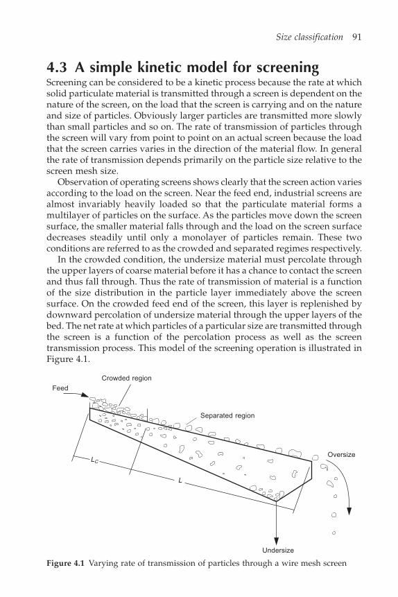
Size classification 91
4.3 A simple kinetic model for screeningScreening can be considered to be a kinetic process because the rate at whichsolid particulate material is transmitted through a screen is dependent on thenature of the screen, on the load that the screen is carrying and on the natureand size of particles. Obviously larger particles are transmitted more slowlythan small particles and so on. The rate of transmission of particles throughthe screen will vary from point to point on an actual screen because the loadthat the screen carries varies in the direction of the material flow. In generalthe rate of transmission depends primarily on the particle size relative to thescreen mesh size.
Observation of operating screens shows clearly that the screen action variesaccording to the load on the screen. Near the feed end, industrial screens arealmost invariably heavily loaded so that the particulate material forms amultilayer of particles on the surface. As the particles move down the screensurface, the smaller material falls through and the load on the screen surfacedecreases steadily until only a monolayer of particles remain. These twoconditions are referred to as the crowded and separated regimes respectively.
In the crowded condition, the undersize material must percolate throughthe upper layers of coarse material before it has a chance to contact the screenand thus fall through. Thus the rate of transmission of material is a functionof the size distribution in the particle layer immediately above the screensurface. On the crowded feed end of the screen, this layer is replenished bydownward percolation of undersize material through the upper layers of thebed. The net rate at which particles of a particular size are transmitted throughthe screen is a function of the percolation process as well as the screentransmission process. This model of the screening operation is illustrated inFigure 4.1.
Figure 4.1 Varying rate of transmission of particles through a wire mesh screen
FeedCrowded region
Separated region
LC
L
Undersize
Oversize
92 Modeling and Simulation of Mineral Processing Systems
Let wi(l) = mass flowrate per unit width of screen of material in size intervali down the screen at distance l from the feed end (kg/ms). wi(l) is related tothe discrete size distribution density function by wi(l) = W(l)pi(l) where W(l)is the total flow of material down the screen per unit width at position l andthe dependence of these functions on position is shown explicitly by theargument l.
If the rate of transmission of particles in size interval i is represented byr(dpi) kg/m2 s, a differential mass balance gives
dw ldl
r dipi
( ) = – ( ) (4.49)
This equation can be integrated if a model for the rate of transmission can bedeveloped.
The rate of transmission will be modeled differently under the crowdedand separated conditions. Accurate models for the crowded condition arecomplex since they must take into account both the stratification andtransmissions processes. A simple but useful model is used here but a morerealistic model is developed in Section 4.3.1.
Unfortunately there is very little data available on the value of thetransmission rate for crowded conditions, r(dp), and its variation with particlesize and with conditions on the screen. It is also dependent on the sizedistribution in the feed.
If the rate of transmission under crowded conditions remains constantalong the screen, Equation 4.49 can be integrated immediately to give
wi(l) = wi(0) – r(dpi)l (4.50)
At the transition between the crowded regime and the separated regimel = Lc
wi(Lc) = wi(0) – r(dpi)Lc (4.51)
with
r(dpi) = k(dpi)Mo piF (4.52)
where Mo is the load on the screen in kg/m2 at the feed end. There is someexperimental evidence to support this assumption of a constant rate oftransmission under crowded conditions.
w L Wb
p k d M p Li cF
iF
pi o iF
c( ) = – ( ) (4.53)
Let M(l) represent the load per unit area of screen surface at a distance l fromthe feed end in kg/m2. The flowrate down the screen W(l) is related to theload on the screen by
W(l) = M(l)u (4.54)
where u is the velocity at which the material travels down the screen:
Size classification 93
w L M up k d M p Li c o iF
pi o iF
c( ) = – ( ) (4.55)
= ( – ( ) )M p u k d Lo iF
pi c
= 1 –( )W
bp
k du
LF
iF pi
c (4.56)
Lc can be defined as the position on the screen at which particles in thesmallest size class just become depleted
L uk dc
pN =
( )(4.57)
The simplest model for the variation of k(dpi) with particle size is:
k du
ku
dh
m d h
d h
pi pipi
pi
( ) = 1 – for <
= 0 for
0 –1(4.58)
where k0/u is the operating parameter. k0/u will depend on the mesh size ofthe screen, its fractional open area and on other operating parameters such asvibration amplitude and frequency.
Under separated conditions, the rate of transmission of particles if size dpis assumed to be proportional to the amount of that material per unit area ofscreen surface
dw ldl
s d M l p lipi i
( ) = – ( ) ( ) ( ) (4.59)
wherepi(l) = the discrete particle size density function of the material on
the screen at distance l from the feed end.s(dpi) = the specific rate of transmission for particles of size dpi
(sec–1)wi(l) is related to M(l) by
wi(l) = pi(l)M(l)u (4.60)
dw ldl
s du
w li pii
( ) = –
( ) ( ) (4.61)
This is easy to integrate and match the individual mass flowrates for eachsize interval at the boundary between the crowded and separated regions:
w l w Ls d
ul Li i c
pic( ) = ( ) exp –
( )( – ) (4.62)
= [ (0) – ( ) ] exp –( )
( – )w r d Ls d
ul Li pi c
pic (4.63)

94 Modeling and Simulation of Mineral Processing Systems
The partition factor can be evaluated from Equation 4.63:
c dw Lw
r d Lw
s du
L L
pii
i
pi c
i
pic
( ) = ( )(0)
= 1 –( )
(0) exp –
( )( – )
(4.64)
The specific rate constant s(dpi)/u can be approximated by the probability ofpassage of a particle during a single contact with the screen. This is usuallycomputed as the ratio of the area of the effective aperture to the total area ofthe screen. In order to pass cleanly through a square mesh opening a sphericalparticle must pass with its center within a square of side h – dp in the centerof the mesh opening. Thus the probability of passage is given by
Ph d
h dh
h d
dh
fdh
rp
w w
p
p
= ( – )
( + )=
( + )1 –
= 1 –
2
2
2
2
2
0
2(4.65)
where f0 is the fraction open area of the screen. This is illustrated inFigure 4.2.
Figure 4.2 Geometrical restrictions on the passage of a particle through square-mesh screen
h
dw
dp
Open area = ( + )
2
2h
h dw
Area for clear passage = ( – )
( + )
2
2
h d
h dp
w
Size classification 95
Ferrara et al. (1988) suggested an empirical functional form:
s du
nfdh
pi pi( ) = 1 –0
/2 (4.66)
where is a constant that should be close to 2. n is the number of presentationsper unit length of bed. Equation 4.66 can be written
s du
sdh
d h
d h
pi pipi
pi
( ) = 2 1 – for <
= 0 for
50 (4.67)
where s50 is the value of s(dpi)/u when the particle size is one half the meshsize. s50 should be proportional to f0
/2 for similar screen types but will alsovary with angle of inclination, vibration amplitude and frequency and themode of vibration.
4.3.1 The Ferrara-Preti-Schena kinetic modelThe modeling of the kinetics of the transmission process under crowdedconditions given in the previous section does not represent the processparticularly well. Ferrara et al. have analyzed an alternative model which isbased on the assumption that the local rate of transmission under crowdedconditions at size dp is proportional to the mass fraction of material of size dpon the screen. This reflects the obvious fact that particle sizes that are notabundant do not transmit large quantities of material.
Equation 4.49 can now be written
dw d ldl
k d p d lp
p p( , )
= – ( ) ( , ) (4.68)
where k(dp) is a kinetic transmission coefficient that is independent of the sizedistribution in the feed.
Using Equation 4.60
dw d ldl
k du
w d lM l
p p p( , ) = –
( ) ( , )( )
(4.69)
It is usual to write this in terms of the total mass of material flowing along thescreen.
W l uM l w d l ddp p( ) = ( ) = ( , )0
(4.70)
dw d ldl
k dw d l
W lp
pp( , )
= – ( ) ( , )
( )(4.71)
This equation is difficult to solve because W(l) is related to the dependent
96 Modeling and Simulation of Mineral Processing Systems
variable w(dp, l) through the integral in Equation 4.70. It is best solved bynoting the formal solution
E d lw d lw d
k d dlW lp
p
pp
l
( , ) = ( , )( , 0)
= exp – ( ) ( )0
(4.72)
and Equation 4.71 becomes
W lE d l
dE d ldl
k dp
pp
( )( , )
( , ) = – ( ) (4.73)
Introduce a new variable
( ) = ( )( )
x k xk dp
(4.74)
where x can represent any particle size.Using Equation 4.72
( ) = ln ( , )ln ( , )
x E x lE d lp
(4.75)
and noting that
W l w x l dx
w x E x l dx
( ) = ( , )
= ( , 0) ( , )
0
0
(4.76)
and
E(x, l) = E(dp, l) (x) (4.77)
Equation 4.73 becomes
0
( )–1( , 0) ( , ) ( , )
= – ( )w x E d ldE d l
dldx k dp
x pp (4.78)
For every screen there will be a particle size D above which the rate oftransmission is zero so that
(x) = 0 for x D (4.79)
The integral in Equation 4.78 can be split into two parts which can be integratedwith respect to l over the range 0 to Lc to give
0
( )( , 0)( )
[ ( , ) – 1] + ( , 0) ln ( , ) = – ( )D
p cx
Dp c p c
w xx
E d L dx w x E d L dx k d L
(4.80)
Size classification 97
This equation can be written in terms of the size distribution in the feed
Wp x
xE d L dxF
D F
p cx( )
( ) [ ( , ) – 1]
0
( )
+ ( ) ln ( , ) = – ( )W P D E d L k d L bF Fp c p c (4.81)
where b represents the width of the screen.In practice this equation is solved using a finite difference approximation
WL b
pE d L W P D E d L k d
F
c j
jF
jipi c
F Fpi c pi
ji [ ( , ) – 1] + ( ) ln ( , ) = – ( ) (4.82)
where
jipj
pi
k dk d
= ( )( )
(4.83)
and the summation is taken only over those classes for which dpj < D.Equation 4.82 is solved for E(dpi, l) for each particle size class.Ferrara et al. propose that k(dp) should be modeled by an equation of the
form
k d kdDp
p( ) = 2 1 –50 (4.84)
with approximately equal to 2. k50 is the rate of transmission of particleswith size equal to 1/2 the mesh size under crowded conditions in the absenceof any other particle sizes. It must be determined by experiment. Anapproximate value can be obtained using the standard screen capacity factorfor undersize transmission evaluated for the mesh size used and 0% oversizeand 100% undersize. Using the Karra formulas this would be given by
k A B50 = 1.6 3.5
1600 tons/hr m2 (4.85)
The partition coefficient at each size is given by Equation 4.64
c d E d Ls d
uL Lpi pi c
pic( ) = ( , ) exp –
( ) ( – ) (4.86)
There is no known way of predicting a priori the value of the length Lc of thescreen over which crowded screening conditions exist. It will be necessary toinvestigate by experiment how the kinetic constants are affected by operatingconditions on the screen before this kinetic model finds any real applicationin practice.
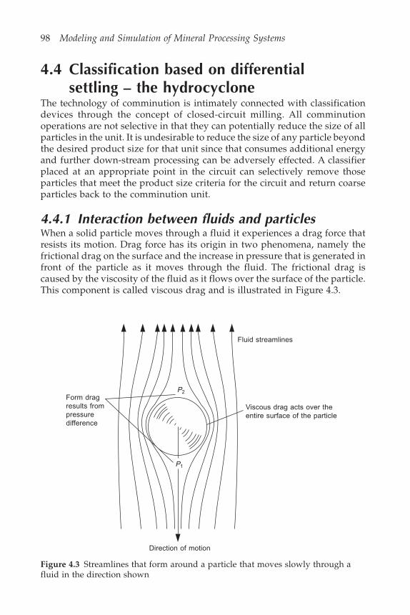
98 Modeling and Simulation of Mineral Processing Systems
4.4 Classification based on differentialsettling – the hydrocyclone
The technology of comminution is intimately connected with classificationdevices through the concept of closed-circuit milling. All comminutionoperations are not selective in that they can potentially reduce the size of allparticles in the unit. It is undesirable to reduce the size of any particle beyondthe desired product size for that unit since that consumes additional energyand further down-stream processing can be adversely effected. A classifierplaced at an appropriate point in the circuit can selectively remove thoseparticles that meet the product size criteria for the circuit and return coarseparticles back to the comminution unit.
4.4.1 Interaction between fluids and particlesWhen a solid particle moves through a fluid it experiences a drag force thatresists its motion. Drag force has its origin in two phenomena, namely thefrictional drag on the surface and the increase in pressure that is generated infront of the particle as it moves through the fluid. The frictional drag iscaused by the viscosity of the fluid as it flows over the surface of the particle.This component is called viscous drag and is illustrated in Figure 4.3.
Figure 4.3 Streamlines that form around a particle that moves slowly through afluid in the direction shown
Fluid streamlines
Viscous drag acts over theentire surface of the particle
Form dragresults frompressuredifference
P2
P1
Direction of motion
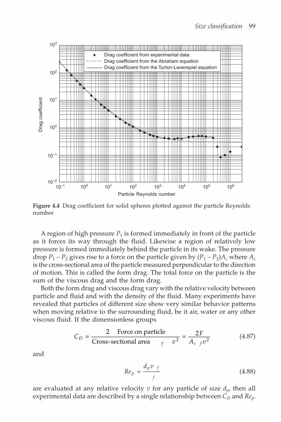
Size classification 99
A region of high pressure P1 is formed immediately in front of the particleas it forces its way through the fluid. Likewise a region of relatively lowpressure is formed immediately behind the particle in its wake. The pressuredrop P1 – P2 gives rise to a force on the particle given by (P1 – P2)Ac where Acis the cross-sectional area of the particle measured perpendicular to the directionof motion. This is called the form drag. The total force on the particle is thesum of the viscous drag and the form drag.
Both the form drag and viscous drag vary with the relative velocity betweenparticle and fluid and with the density of the fluid. Many experiments haverevealed that particles of different size show very similar behavior patternswhen moving relative to the surrounding fluid, be it air, water or any otherviscous fluid. If the dimensionless groups
Cv
FA v
Df c f
= 2 Force on particle
Cross-sectional area = 2
2 2(4.87)
and
Red v
pp f
f = (4.88)
are evaluated at any relative velocity v for any particle of size dp, then allexperimental data are described by a single relationship between CD and Rep.
Drag coefficient from experimental dataDrag coefficient from the Abraham equationDrag coefficient from the Turton-Levenspiel equation
10–1 100 101 102 103 104 105 106
Particle Reynolds number
Dra
g co
effic
ient
103
102
101
100
10–1
10–2
Figure 4.4 Drag coefficient for solid spheres plotted against the particle Reynoldsnumber
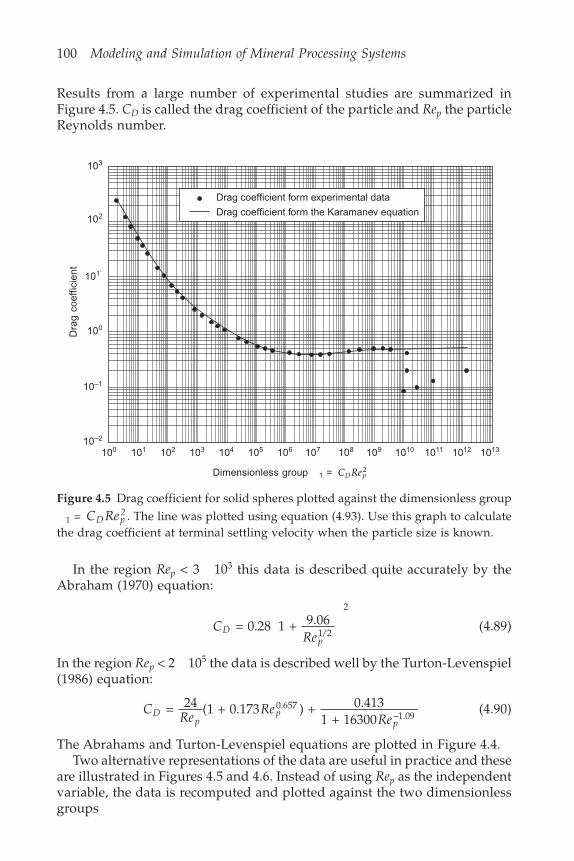
100 Modeling and Simulation of Mineral Processing Systems
Results from a large number of experimental studies are summarized inFigure 4.5. CD is called the drag coefficient of the particle and Rep the particleReynolds number.
Figure 4.5 Drag coefficient for solid spheres plotted against the dimensionless group
1 = C ReD p2 . The line was plotted using equation (4.93). Use this graph to calculate
the drag coefficient at terminal settling velocity when the particle size is known.
Drag coefficient form the Karamanev equation
Drag coefficient form experimental data
103
102
101`
100
10–1
10–2
100 101 102 103 104 105 106 107 108 109 1010 1011 1012 1013
Dimensionless group 1 = C ReD p2
Dra
g co
effic
ient
In the region Rep < 3 103 this data is described quite accurately by theAbraham (1970) equation:
CRe
Dp
= 0.28 1 + 9.061/2
2
(4.89)
In the region Rep < 2 105 the data is described well by the Turton-Levenspiel(1986) equation:
CRe
ReRe
Dp
pp
= 24 (1 + 0.173 ) + 0.4131 + 16300
0.657–1.09
(4.90)
The Abrahams and Turton-Levenspiel equations are plotted in Figure 4.4.Two alternative representations of the data are useful in practice and these
are illustrated in Figures 4.5 and 4.6. Instead of using Rep as the independentvariable, the data is recomputed and plotted against the two dimensionlessgroups
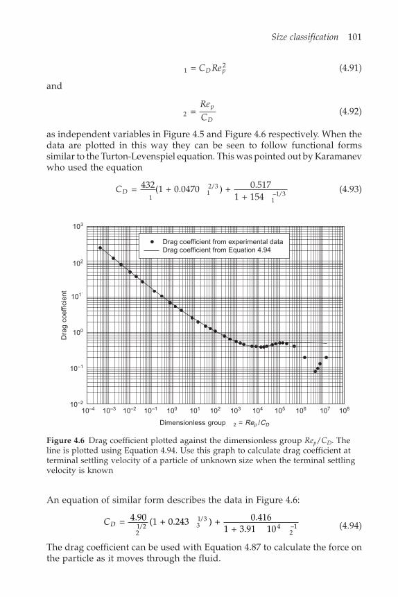
Size classification 101
Drag coefficient from experimental dataDrag coefficient from Equation 4.94
12 = C ReD p (4.91)
and
2 = ReC
p
D(4.92)
as independent variables in Figure 4.5 and Figure 4.6 respectively. When thedata are plotted in this way they can be seen to follow functional formssimilar to the Turton-Levenspiel equation. This was pointed out by Karamanevwho used the equation
CD = 432(1 + 0.0470 ) + 0.5171 + 1541
12/3
1–1/3
(4.93)
Figure 4.6 Drag coefficient plotted against the dimensionless group Rep/CD. Theline is plotted using Equation 4.94. Use this graph to calculate drag coefficient atterminal settling velocity of a particle of unknown size when the terminal settlingvelocity is known
An equation of similar form describes the data in Figure 4.6:
CD = 4.90 (1 + 0.243 ) + 0.4161 + 3.91 102
1/2 31/3
42–1 (4.94)
The drag coefficient can be used with Equation 4.87 to calculate the force onthe particle as it moves through the fluid.
103
102
101`
100
10–1
10–2
10–4 10–3 10–2 10–1 100 101 102 103 104 105 106 107 108
Dimensionless group 2 = Rep /CD
Dra
g co
effic
ient
102 Modeling and Simulation of Mineral Processing Systems
Force = 2
2Cv AD
f c (4.95)
4.5 Terminal settling velocityIf a particle falls under gravity through a viscous fluid it will accelerate for ashort while but as the particle moves faster the drag force exerted by the fluidincreases until the drag force is just equal to the net gravitational force lessthe buoyancy that arises from the immersion of the particle in the fluid.
The terminal settling velocity vT can be evaluated by balancing the dragand buoyancy forces
p s fD
f T cgC
v A( – ) = 2
2 (4.96)
where p is the volume of the particle.
4.5.1 Settling velocity of an isolatedspherical particle
When the particle is spherical, the geometrical terms in Equation 4.96 can bewritten in terms of the particle diameter
6 ( – ) =
2 42 2d g
Cv dp
3s f
Df T p (4.97)
The drag coefficient at terminal settling velocity is given by
Cv
gdDs f
f Tp* = 4
3( – )
2(4.98)
and the particle Reynolds number at terminal settling velocity is given by
Red v
pp T f
f* = (4.99)
It is not possible to solve Equation 4.97 directly because CD is a function ofboth vT and the particle size dp through the relationship shown in Figure 4.4or either of the Abraham or Turton-Levenspiel equations. Two different solutionprocedures are commonly required in practice: the calculation of the terminalsettling velocity for a particle of given size or the calculation of the size of thespherical particle that has a prespecified terminal settling velocity. Theseproblems can be solved without recourse to trial and error methods byconsidering the two dimensionless groups 1 and 2 both evaluated at theterminal settling velocity.
Size classification 103
12
2
2
23 3
* = * * = 43
–
43
( – ) = *
C Regd
v
d v
gd d
D ps f
f
p
T
p T f
f
s f ff
p p
(4.100)
and
2
23 3* =
*
*34 ( – )
= *Re
C gv V
p
D
f
s f fT T (4.101)
dp* and VT* are called the dimensionless diameter and the dimensionless
terminal settling velocity of a sphere respectively. dp* can be evaluated from
a knowledge of the properties of the fluid and the size of the particle. dp* is
independent of the terminal settling velocity. VT* is independent of the particlesize and can be evaluated if the terminal settling velocity is known. 1* isoften called the Archimedes number which is usually represented by thesymbol Ar.
From the definition of 1* and 2* given in Equations 4.100 and 4.101, thefollowing relationships are easily derived.
Re d Vp p T* = ( * * ) = * *1 21/3 (4.102)
CRe
Re
d
VD
p
p
p
T
* = *
* =
*
* =
*
*2
12 2
(4.103)
Re C Vd
Cp D T
p
D
* = * * = *
*3
31/2
(4.104)
The drag coefficient at terminal settling velocity can be calculated easily fromFigure 4.5 or Equation 4.93 if the dimensionless diameter of the particle isknown. It is then a simple matter to evaluate the terminal settling velocityfrom Equation 4.97 or more conveniently from Equation 4.103.
The diameter of the particle that has known terminal settling velocity canbe calculated using a similar procedure. In this case the dimensionless settlingvelocity VT* is calculated using Equation 4.101 and the drag coefficient atterminal settling velocity can then be calculated from Equation 4.94 or readfrom Figure 4.6. In either case the required variable can be calculated directlyfrom Equation 4.97 once CD
* is known or more conveniently from Equation4.103.
A similar solution procedure can be obtained using the Abraham equation
104 Modeling and Simulation of Mineral Processing Systems
starting from Equation 4.102. The Abraham equation may be solved directlyto give the dimensionless terminal settling velocity once dp* is known.
VRe
C
d V
d V
Tp
D
p T
p T
* = *
* =
* *
0.28 1 + 9.06( * * )
3
1/2
2 (4.105)
1 + 9.06( * * )
= *
0.28 *1/2
1/2
1/2d V
d
Vp T
p
T
(4.106)
This equation can be re-arranged to show more clearly the relationship betweenVT* and dp*
0.28 * * + 9.06 0.28 * – * = 01/2 1/2 1/2 1/2V d V dT P T p (4.107)
This equation can be solved for VT* in terms of dp* or for dp* in terms of VT* .Either way the solution procedure is straightforward because Equation 4.107
is quadratic in the variables VT*1/2 and dp*1/2 .
The solutions are:
Vd*
dTp
p* = 20.52[(1 + 0.0921 * ) – 1]3/2 1/2 2 (4.108)
dV
Vp
TT* = 0.070 1 + 68.49
*+ 1 *
3/2
1/2 2
2 (4.109)
The drag coefficient at terminal settling velocity is related to dp* and VT* mostdirectly by Equation 4.103.
These solutions are due to Concha and Almendra (1979).This approach to the analysis of terminal settling velocity provides
straightforward linear procedures for the calculation of terminal settling velocityor particle size. No inconvenient iterative calculations are required. Illustrativeexamples 4.1 and 4.2 demonstrate their application.
Illustrative example 4.1 Terminal settling velocityCalculate the terminal settling velocity of a glass sphere of diameter 0.1 mmin a fluid having density 982 kg/m3 and viscosity 0.0013 kg/ms. Density ofglass is 2820 kg/m3. Also calculate the drag coefficient at terminal settlingvelocity.
SolutionSince the particle size is known, calculate dp* .
Size classification 105
13
3
2* = * = 4
3( – )
dg d
ps f f p
f
= 43
(2820 – 982) 982 9.81 (0.1 10 )(0.0013)
–3 3
2
= 13.97
Using the Karamanev modification to the Turton-Levenspiel equation,
CD* = 432*
(1 + 0.0470 * ) + 0.5171 + 154 1
12/3
1–1/3
= 39.355 + 0.008 = 39.36
Check this on the graph of CD vs 1 (Figure 4.5)
ReC
pD
* = *
* = 13.97
39.36= 0.5961
1/21/2
Check this on the CD vs Rep graph (Figure 4.4)
T pf
p fRe
d = * = 0.596 0.0013
0.1 10 982 = 7.89 10 m/s–35
–3
Alternatively use the Concha-Almendra procedure
dp* = (13.97) = 2.4081/3
Vd
dTp
p* = 20.52*
[(1 + 0.0921 * ) – 1]3/2 1/2 2
= 0.217
Re d Vp p T* = * * = 2.408 0.217 = 0.522
Tp f
p f
Red
= *
= 0.522 0.0013. 982
= 6.91 10 m/s–3–3
0 1 10
The drag coefficient at terminal settling velocity is calculated from
Cd
Vd
p
T
* = *
*2.408
0.217 = 51.1
2 2
Illustrative example 4.2 Size of settling particleFind the size of a spherical particle of glass that has a terminal settling velocityof 7.4 mm/s in a fluid of density 982 kg/m3 and viscosity 0.0013 kg/ms.Density of glass is 2820 kg/m3.
106 Modeling and Simulation of Mineral Processing Systems
SolutionSince the terminal settling velocity is known, start the calculation with VT* .
23
2
T3* = * = 3
4 ( – )V
gTf
s f f
= 34
982 (7.4 10 )(2820 – 982) 0.0013 9.81
= 0.01252 –3 3
CD* = 4.90*
(1 + 0.243 * ) + 0.4161 + 3.91 1 *2
1/2 21/3
2–10 4
= 46.29 + 1.33 10–7 = 46.29
Re C Vp D T* = * * = 46.29 0.0125 = 0.5793
dRe
pp f
T f =
* = 0.579 0.0013
7.4 10 982 = 1.04 10 m–3
– 4
Alternatively, the Concha-Almendra method can be used.
dV
Vp
TT* = 0.070 1 + 68.49
* + 1 * = 2.504
3/2
1/2 2
2
Re* d V*p p T = * = 2.504 (0.0125) = 0.5811/3
dRe
pp f
T f =
* = 1.04 10 m–4
4.5.2 Stokes’ lawWhen the relative velocity between the particle and the fluid is very low, therelationships that define the interaction between the fluid and the particlebecome very simple. Under this extreme condition
CReD
p = 24 (4.110)
The force experienced by the particle is given by Equation 4.87
Force = 12Ad
vc
pf (4.111)
The terminal settling is obtained by substitution of this equation into Equation4.96

Size classification 107
6( – ) = 24
2 43 2 2d g
Rev dp s f
pf T p (4.112)
v gdTs f
fp =
–18
2 (4.113)
This is known as Stokes’ law of settling. Stokes’ law is particularly useful forthe analysis of the motion of very small particles. It should not be used if theparticle Reynolds number is greater than 1.0.
Illustrative example 4.3Use Stokes’ law to calculate the terminal settling velocity of a glass sphere ofdiameter 0.1 mm in a fluid having density 982 kg/m3 and viscosity 0.0013kg/ms. Density of glass is 2820 kg/m3.
SolutionStokes’ law
Ts f
fpgd =
–18
2
= 2820 – 98218 0.0013
9.81 (0.1 10 )–3 2
= 7.71 10–3 m/s
Calculate the Reynolds number at terminal settling velocity to establish whetherStokes’ law can be applied.
Red
pp T f
f* =
=0.1 10 7.71 10 9.82
0.0013 = 0.582
–3 –3
This satisfies the condition Rep < 1.0 for the application of Stokes’ law.
4.5.3 Isolated isometric particles of arbitrary shapeWhen the particles are not spherical but at least isometric (i.e. they haveroughly equal dimensions in three orthogonal directions) useful correlationshave been developed by Concha and Barrientos (1986). There are two factorsthat make the non-spherical particles differ from their spherical counterparts:the surface area per unit volume will be larger giving rise to larger surfacedrag and the irregular shape of the particle gives rise to oscillatory andvibratory motions as the particle settles through the fluid. The former effectis significant at all particle Reynolds numbers while the latter effect is significantonly under turbulent flow conditions.
The particle size is now defined as the equivalent volume diameter.
108 Modeling and Simulation of Mineral Processing Systems
dep
= 6 1/3v
(4.114)
which is the diameter of the sphere having the same volume as the particle.Concha and Barrientos define a modified drag coefficient and a modifiedparticle Reynolds number as
CC
f fDMD
A C =
( ) ( )(4.115)
and
ReRe
f fM
p
B D =
[ ( ) ( )]2 (4.116)
In these equations represents the particle sphericity and the densityratio
= Surface area of sphere with equal volume
Surface area of particle(4.117)
=2d
ae
p
= s
f(4.118)
The functions fA, fB, fc and fD account for the effect of sphericity and densityratio on the drag coefficient and the particle Reynolds number.
The Abrahams equation is modified in a simple way to allow for non-spherical particles.
CRe
DMM
= 0.284 1 + 9.061/2
2
(4.119)
The empirical functions proposed by Concha and Barrientos are given by
fA ( ) = 5.42 – 4.75
0.67(4.120)
f fB A( ) = 0.843 ( ) log 0.065
–1/2
(4.121)
fC( ) = –0.0145 (4.122)
fD( ) = 0.00725 (4.123)
Note that
fA(1) = fB(1) = fC(1) = fD(1) = 1.0 (4.124)
Size classification 109
These functions allow the definition of modified dimensionless particle sizeand dimensionless settling velocity as follows:
d d*eM e* = ( ( )) ( ( ))2/3 2/3 (4.125)
and
VV
mT* = *
( ) ( ) ( ) ( )2/3 2/3(4.126)
where de* and VT* are evaluated from Equations 4.100 and 4.101 using de
rather than dp in Equation 4.100. The new functions , , and are relatedto fA, fB, fc and fD as follows:
( ) = ( )2fB (4.127)
( ) = ( ( ) ( ))1/2 2 –1f fA B (4.128)
( ) = ( )2fD (4.129)
( ) = ( ( ) ( )1/2 2f fc D )–1 (4.130)
With these definitions of ( ), ( ), ( ) and ( ), it is easy to show that themodified variables satisfy the same consistency relationships 4.102 and 4.103at terminal settling velocity.
Re d VM M M eM M* = ( * * ) = * *1 21/3 (4.131)
and
CRe
Red
VDM
M
M
M
M
eM
M
= *
* =
* =
*
*2
12 2
(4.132)
With these definitions the modified dimensionless terminal settling velocityis related to the modified dimensionless particle diameter by
Vd
dMeM
em* = 20.52*
[(1 + 0.0921 * ) – 1]3/2 1/2 2(4.133)
and
dV
VeM
MM
* = 0.070 1 + 68.49*
+ 1 *3/2
1/2 2
2 (4.134)
which are identical in form to Equations 4.108 and 4.109. In practice it may bemore convenient to work with VT* and de* and then the relationship between
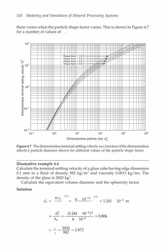
110 Modeling and Simulation of Mineral Processing Systems
them varies when the particle shape factor varies. This is shown in Figure 4.7for a number of values of .
Figure 4.7 The dimensionless terminal settling velocity as a function of the dimensionlesseffective particle diameter shown for different values of the particle shape factor
102
101
100
10–1
10–2
10–1 100 101 102 103 104
Dimensionless particle size d p*
Dim
ensi
onle
ss t
erm
inal
set
ting
velo
city
VT*
Shape factor = 1.0Shape factor = 0.9Shape factor = 0.8Shape factor = 0.6
Illustrative example 4.4Calculate the terminal settling velocity of a glass cube having edge dimension0.1 mm in a fluid of density 982 kg/m3 and viscosity 0.0013 kg/ms. Thedensity of the glass is 2820 kg3.
Calculate the equivalent volume diameter and the sphericity factor.
Solution
dv
ep
= 6
= 6 1 = 1.241 10 m1/3 1/3
–40 12–
= = (1.241 10 )
6 10 = 0.806
2 –4 2
–8
da
e
p
= = 2820982
= 2.872s
f

Size classification 111
fA ( ) = 5.42 – 4.75
0.67 = 2.375
f fB ( ) = 0.843 ( ) log 0.065
–1/2
= 0.676
fc( ) = 0.985
( ) = ( ) = 0.4572fB
( ) = ( ( ) ( )) = 1.4211/2 2 –1f fA B
( ) = = 1.0152fD
( ) = ( ( ) ( ) ) = 0.9921/2 2 –1f fc D
dg
de s f ff
e* = 43
( – ) = 2.9892
1/3
d deM e* = * ( ( )) ( ( )) = 3.7572/3 2/3
Vd
dmeM
eM* = 20.52*
[(1 + 0.0921 * ) – 1]3/2 1/2 2
= 0.467
V VT M* = * ( ) ( ) ( ) ( )2/3 2/3
= 0.273
This combination of de* and VT* can be checked on Figure 4.7.
T Tf
s f fV
g = * 3
4 ( – )
2 –1/3
= 8.70 10–3 m/s
4.5.4 General principles of the operation of thehydrocyclone
The principle of operation of the hydrocyclone is based on the concept of theterminal settling velocity of a solid particle in a centrifugal field. The conditionsin an operating hydrocyclone can be described by reference to Figures 4.8and 4.9. The feed enters tangentially into the cylindrical section of the
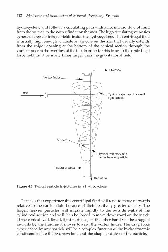
112 Modeling and Simulation of Mineral Processing Systems
hydrocyclone and follows a circulating path with a net inward flow of fluidfrom the outside to the vortex finder on the axis. The high circulating velocitiesgenerate large centrifugal fields inside the hydrocyclone. The centrifugal fieldis usually high enough to create an air core on the axis that usually extendsfrom the spigot opening at the bottom of the conical section through thevortex finder to the overflow at the top. In order for this to occur the centrifugalforce field must be many times larger than the gravitational field.
Vortex finder
Overflow
Typical trajectory of a smalllight particle
Typical trajectory of alarger heavier particle
Underflow
Spigot or apex
Air core
Inlet
Figure 4.8 Typical particle trajectories in a hydrocyclone
Particles that experience this centrifugal field will tend to move outwardsrelative to the carrier fluid because of their relatively greater density. Thelarger, heavier particles will migrate rapidly to the outside walls of thecylindrical section and will then be forced to move downward on the insideof the conical wall. Small, light particles, on the other hand will be draggedinwards by the fluid as it moves toward the vortex finder. The drag forceexperienced by any particle will be a complex function of the hydrodynamicconditions inside the hydrocyclone and the shape and size of the particle.
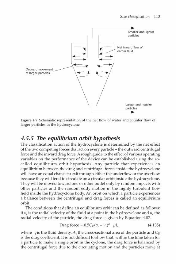
Size classification 113
4.5.5 The equilibrium orbit hypothesisThe classification action of the hydrocyclone is determined by the net effectof the two competing forces that act on every particle – the outward centrifugalforce and the inward drag force. A rough guide to the effect of various operatingvariables on the performance of the device can be established using the so-called equilibrium orbit hypothesis. Any particle that experiences anequilibrium between the drag and centrifugal forces inside the hydrocyclonewill have an equal chance to exit through either the underflow or the overflowbecause they will tend to circulate on a circular orbit inside the hydrocyclone.They will be moved toward one or other outlet only by random impacts withother particles and the random eddy motion in the highly turbulent flowfield inside the hydrocyclone body. An orbit on which a particle experiencesa balance between the centrifugal and drag forces is called an equilibriumorbit.
The conditions that define an equilibrium orbit can be defined as follows:if vr is the radial velocity of the fluid at a point in the hydrocyclone and ur theradial velocity of the particle, the drag force is given by Equation 4.87.
Drag force = 0.5CD(vr – ur)2f Ac (4.135)
where f is the fluid density, Ac the cross-sectional area of the particle and CDis the drag coefficient. It is not difficult to show that, within the time taken fora particle to make a single orbit in the cyclone, the drag force is balanced bythe centrifugal force due to the circulating motion and the particles move at
Larger and heavierparticles
Outward movementof larger particles
Net inward flow ofcarrier fluid
Smaller and lighterparticles
Figure 4.9 Schematic representation of the net flow of water and counter flow oflarger particles in the hydrocyclone
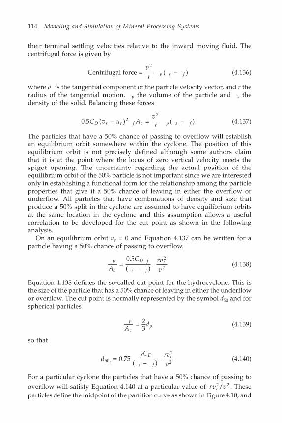
114 Modeling and Simulation of Mineral Processing Systems
their terminal settling velocities relative to the inward moving fluid. Thecentrifugal force is given by
Centrifugal force = ( – )2v
r p s f (4.136)
where v is the tangential component of the particle velocity vector, and r theradius of the tangential motion. p the volume of the particle and s thedensity of the solid. Balancing these forces
0.5 ( – ) = ( – )22
C v u AvrD r r f c p s f (4.137)
The particles that have a 50% chance of passing to overflow will establishan equilibrium orbit somewhere within the cyclone. The position of thisequilibrium orbit is not precisely defined although some authors claimthat it is at the point where the locus of zero vertical velocity meets thespigot opening. The uncertainty regarding the actual position of theequilibrium orbit of the 50% particle is not important since we are interestedonly in establishing a functional form for the relationship among the particleproperties that give it a 50% chance of leaving in either the overflow orunderflow. All particles that have combinations of density and size thatproduce a 50% split in the cyclone are assumed to have equilibrium orbitsat the same location in the cyclone and this assumption allows a usefulcorrelation to be developed for the cut point as shown in the followinganalysis.
On an equilibrium orbit ur = 0 and Equation 4.137 can be written for aparticle having a 50% chance of passing to overflow.
p
c
D f
s f
r
AC rv
v =
0.5( – )
2
2 (4.138)
Equation 4.138 defines the so-called cut point for the hydrocyclone. This isthe size of the particle that has a 50% chance of leaving in either the underflowor overflow. The cut point is normally represented by the symbol d50 and forspherical particles
p
cpA
d = 23
(4.139)
so that
dC rv
vc
f D
s f
r50
2= 0.75
( – ) 2 (4.140)
For a particular cyclone the particles that have a 50% chance of passing tooverflow will satisfy Equation 4.140 at a particular value of rv vr
2/ 2 . Theseparticles define the midpoint of the partition curve as shown in Figure 4.10, and

Size classification 115
Equation 4.140 provides a correlation for the cut point as a function of particleproperties.
Figure 4.10 Typical partition curves for a hydrocyclone
1.0
0.75
0.25
0.0
Rec
over
y to
und
erflo
w
Ideal partitioncurve e (dp )
d50
d25
d50c
d75
Particle size
The drag force experienced by a particle due to the relative motion betweenit and the fluid is the key to using the equilibrium orbit theory as a basis formodeling the behavior of the hydrocyclone. It is known that these relativevelocities are small and the particle Reynolds number is usually so low thatit is commonly assumed that the drag force can be calculated from the formulafor the slow relative motion between a sphere and a Newtonian fluid. This isthe well-known Stokes formula. This approach neglects two importantphenomena: the highly turbulent nature of the fluid inside the hydrocycloneand the relatively high concentration of particles. Thus the use of Stokes’flow theories which assumes that only a single isolated particle is present isnot very realistic.
Four limiting cases can be considered: isolated particles in a laminarflow field (Stokes regime), isolated particles in a turbulent flow field(Newton regime), interacting particles in a laminar flow field (Blake-Kozenyregime) and interacting particles in a turbulent flow field (Burke-Plummerregime).
0.5
Actual partitioncurve c (dp )
116 Modeling and Simulation of Mineral Processing Systems
The drag coefficient in Equation 4.140 is a function of the particle size andshape and the environment that the particle finds on its equilibrium orbit.Each of the four environments defined above give different expressions forCD.
Stokes regimeIn this regime the particles do not interact with each other and are surroundedby fluid in laminar motion. The drag coefficient is given by Equation 4.110.
CReD
p = 24
24( – )
f
p r r fd v u(4.141)
=24 f
p r fd v on an equilibrium orbit
Substituting in Equation 4.140 and noting that dp = d50c on an equilibriumorbit:
dd
rvv
f
s f
r50c
50 2 = 1 .
( – )8 0
dK rv
vcs f
r502 1
2 = ( – ) (4.142)
Newtonian regimeIn this regime isolated particles are surrounded by fluid in turbulent motionand from the Abraham equation:
CD = 0.28 (4.143)
Substituting in Equation 4.141:
drvv
dK rv
v
cf
s f
r
cs f
r
50
2
2
502
2
2
= 0.22 ( – )
= ( – )
(4.144)
The two limiting cases for the equilibrium orbit hypothesis (Equations 4.142and 4.144) indicate that the variation of d50c with the density difference andwith the volumetric feed rate should take the form:
dKD
Qc
ck
s fm
cn50 =
( – ) (4.145)
Size classification 117
where m and k are constants having a values between 0.5 and 1, and n is aconstant between 0 and 0.5. The lower limit of 0.5 for m and k representslaminar flow conditions and turbulence inside the hydrocyclone will giverise to higher values of m and k and lower values of n.
Experimental observations have shown that the ratio vr/v is independentof total flow rate at every point inside the hydrocyclone and the assumptionof turbulent flow (Equation 4.144) indicates that d50c should be at most aweak function of the total flow rate while the assumption of laminar flowconditions (Equation 4.142) indicates that d50c should be inversely proportionalto the square root of the volumetric flow rate. Under turbulent conditions,d50c may be expected to increase linearly with the cyclone diameter.
No one set of assumptions is likely to describe the operating behavior ofthe hydrocyclone under all conditions. Consequently only comparativelycrude empirical correlations are currently available for the prediction of thevariation of d50c with hydrocyclone geometry and operating conditions.
4.5.6 Empirical performance models forhydrocyclones
Unfortunately no classifier operates perfectly and classifiers will not dividea population of particles into two groups separated at a definite and particularsize. All classifiers are characterized by a distribution function which givesthe efficiency of separation at any size and the distribution function is moreor less sharp depending on the efficiency of separation. A typical classificationcurve is shown in Figure 4.10. This is called the partition curve (sometimescalled the Tromp curve) and it shows the fraction of particles at a particularsize that will be partitioned to the coarser fraction. The S shaped curve istypical of all practical classifiers and a variety of quantitative expressionshave been used to describe the shape of the curve.
A characteristic of virtually all practical classifiers is the phenomenon ofshort circuiting. All classifiers exploit some physical process to separate particleson the basis of size. This will be the differential settling velocity in a viscousfluid in spiral, rake and hydrocyclone classifiers or the physical sieving actionin a screening operation. Some particles pass through the equipment withoutbeing subjected to the physical separation action. In practice it is only theshort circuiting of the fine particles to the coarser product stream that issignificant. This shows up as a non-zero intersection on the partition axis atzero size. In the hydrocyclone this is due to the water carrying fine particlesinto the boundary layer on the outer wall of the conical section and dischargingthem with the underflow. In other classifiers such as spiral, rake and thevarious screening operations, fine particles are physically carried with thelarge particles into the coarse product stream.
This short circuit effect can easily be accounted for by reference to Figure4.11.
If the ideal classification action of the unit is described by classificationfunction e(dp) and a fraction of the feed short circuits directly to the
118 Modeling and Simulation of Mineral Processing Systems
coarser product then a simple mass balance gives the actual classificationcurve as
c(dp) = + (1 – )e(dp) (4.146)
e(dp) is called the corrected classification function and c(dp) the actualclassification function.
The important parameter that characterizes the operation of the classifieris the size at which e(dp) is 0.5. This size is usually called the corrected d50c(corrected since the effect of the short circuit flow has been eliminated asshown in Figure 4.10). d50c and d50 are defined by the equations
e(d50c) = 0.5 (4.147)
and
c(d50) = 0.5 (4.148)
Fine product
Ideal classifier
Actual classifier
Coarse product
Short-circuit flow
Feed
Figure 4.11 A hydrocyclone with short circuit to the underflow

Size classification 119
d50 is clearly an indicator of the size at which the classifier cuts the particlepopulation.
Although phenomenological models have been developed for the mainclassifier types, no completely satisfactory procedure exists for the calculationof the classification function in any of the main types of classifier. In thehydrocyclone the function is determined primarily by the turbulent dispersionwithin the centrifugal velocity field in the conical section and this has been afertile field of research for many years. On the various types of screeningdevices, the classification function is determined by the kinetics of thetransmission process of particles through the apertures of the screen. Theseprocesses have been comprehensively studied but it is not yet possible tomake accurate calculations of the classification function in terms of thedimensions of and operating load on the classifier. However, a number ofuseful empirical functional forms are available to describe the ideal classificationfunction. The most commonly used are:
1. Rosin-Rammler
e(dp) = 1 – exp(–0.693x ) (4.149)
2. Exponential sum
e dx
xp( ) = exp( ) – 1
exp( ) + exp( ) – 2(4.150)
3. Logistic
e(dp) = 1/(1 + x– ) (4.151)
In these equations x = dp/d50c and is a parameter that quantifies the sharpnessof the classification. It is relatively easy to appreciate the sharpness ofclassification in terms of the sharpness index defined by
SI = d25/d75 (4.152)
with e(d25) = 0.25 and e(d75) = 0.75. SI has a value between 0 and 1 with lowvalues indicating poor and inefficient separation while a value of 1.0 indicatesperfect classification at the cut size d50c .
The parameter is related to the sharpness index for each case givenabove as follows:
1. Rosin-Rammler
(SI)– = 4.819 (4.153)
SI = exp(–1.572/ ) (4.154)
= – 1.572ln( )SI
(4.155)
2. Exponential sum
SI = ln[exp + 2)/3]ln[3 exp – 2]
(4.156)
120 Modeling and Simulation of Mineral Processing Systems
is usually quite large and Equation 4.156 can be solved approximately for in terms of SI as follows:
= 1.099 (1 + )(1 – )
SISI
(4.157)
3. Logistic
(SI)– = 9 (4.158)
SI = exp(–2.1972/ ) (4.159)
= –2.1972ln( )SI
(4.160)
These functions are useful for the quantitative description of the behavior ofthe various classification units but it is necessary to evaluate the threeparameters , d50 and in terms of the physical dimensions and the actualoperating conditions relevant to the unit in question.
Illustrative example 4.5 Effect of particle densityA hydrocyclone was found to have a corrected classification curve given by
e(dp) = 1/(1 + x– )
where x = dp/d50c.When processing a quartz slurry, d50c = 16.5 m and SI = 0.72.Calculate the recovery of 10 m particles to overflow when this hydrocyclone
treats a magnetite slurry under comparable conditions. Density of quartz is2670 kg/m3 and that of magnetite is 5010 kg/m3. Recovery of water tounderflow is 18.5% in both cases.
Solution
For magnetite d c
m
50 = 16.5 2670 – 10005010 – 1000
Evaluate this for the two limiting cases: Stokes regime and fully turbulentregime.
Stokes regime: m = 0.5 d50c = 10.65 mTurbulent regime m = 1.0 d50c = 6.87 m
Classification function C(dpi) = + (1 – ) 11 + –x
= 0.185 + (1 – 0.185) 1
1 + 1010.65
– 6.686
= 0.185 + (1 – 0.185) 0.396
= 0.5079
Size classification 121
For the logistic function = – 2.1972ln( )
= – 2.1972ln(0.72)SI
= 6.689
Recovery to overflow = 1 – 0.5079 = 49.2%
4.5.7 The Plitt model for the hydrocycloneThe classification action of the hydrocyclone depends on a balance betweenthe hydrodynamic drag forces that tend to convect the particle toward theaxis and the centrifugal force that tends to move the particle outward towardsthe wall of the cone. The d50 size will be determined for the particle that findsthese two forces in balance and this gives rise to the equilibrium orbit hypothesisthat is discussed in Section 4.5.5. This hypothesis allows some generalconclusion to be drawn for predicting d50 as a function of hydrocyclonegeometry and operating conditions.
The performance of the hydrocyclone is strongly influenced by the shortcircuit to underflow and this is determined by the volumetric flow splitbetween over- and underflow. The volumetric flow split, S, is a functionprimarily of the ratio of spigot to vortex finder diameters but is also a strongfunction of the total feed rate. As the flow rate through the hydrocycloneincreases, the diameter of the air core increases choking off the underflow.This effect has not been comprehensively studied and we use a correlationdeveloped by Plitt (1976) based on experimental data.
Sa D D D D h
D Hu o
bu o
c d
cf g
= ( / ) ( + ) exp (0.54 )2 2
(4.161)
whereS = volumetric flow rate in underflow/volumetric flow rate in
overflowDu = spigot diameterDo = vortex finder diameterDc = cyclone diameter
= volume fraction solids in the feedh = vortex finder to spigot distance
H = slurry feed headThe following values are recommended for hydrocyclones operating withfree discharge: a = 3.79, b = 3.31, c = 0.36, d = 0.54, f = 1.11, g = 0.24. The inversedependence on the feed head H should be noted. As the head increases theflow through the hydrocyclone increases, the centrifugal field increases andthe air core expands choking off the discharge from the spigot.
The following recoveries are defined:
Rv = volumetric flowrate in the underflow/volumetric flowrate in the feedRf = recovery of fluid phase to the underflowRs = recovery of solid phase to the underflow.

122 Modeling and Simulation of Mineral Processing Systems
The volumetric recovery to underflow is related to S by:
R SSv =
+ 1(4.162)
The bypass fraction is assumed to be equal to the fraction of water thatreports to the underflow Rf, and this is related to the recovery of solids Rs by
Rv = Rs + Rf(1 – ) (4.163)
= = –
1 –R
R Rf
v s (4.164)
Rs is determined from Equation 4.29 by the actual classification functionwhich in turn is itself a function of Rf
R c d ps i pi iF = ( ) (4.165)
where piF is the particle size distribution in the feed.
Using Equation 4.146
R R R e d ps i f f pi iF = [ + (1 – ) ( )]
= + (1 – ) ( ) R R e d pf f i pi iF (4.166)
Substitution into Equation 4.164 and simplifying gives
RR e d p
e d pf
v i pi iF
i pi iF
= – ( )
1 – ( )(4.167)
Thus the hydrocyclone performance is completely determined if the correctedclassification function e(dp) is known together with the volumetric flow split S.
The Rosin-Rammler model 4.149 is used to describe the partition function,which requires two parameters, d50 and . Plitt has correlated these parametersin terms of the cyclone geometry and the operating variables as follows:
daD D D
D h Qc
cb
ic
od
uf g i
s f50 0.5
= exp [6.3 ]
( – ) (4.168)
Di is the inlet diameter and Q the volumetric flowrate to the cyclone.Recommended values for the constants are a = 2.69 103 and b = 0.46, c =
0.6, d = 1.21, f = 0.71, g = 0.38, i = 0.45. With this value of a, d50c from Equation4.168 will be in microns. Comparison of Equation 4.168 with Equation 4.145indicates that Plitt’s model for d50c is consistent with the main conclusionsdrawn from the equilibrium orbit hypothesis in that d50c varies roughly inproportion to the cyclone diameter (cyclone size to the power b + c + d – f –g = 1.18) and inversely with feed rate to a power less than 1. The 0.5 power
Size classification 123
dependence on s – f indicates that the interaction between particles andfluid is governed by Stokes’ law but slightly higher values can be used.
The parameter in Equation 4.149 is correlated by:
= exp (– 1.58 )2
aD hQ
Rcb
v (4.169)
Recommended values for the constants are a = 2.96 and b = 0.15. This equationreveals that the efficiency of separation depends on the volumetric recoveryRv but is a comparatively weak function of the cyclone size particularly whenthe feed rate Q is properly matched to the cyclone size.
It is useful to convert Equation 4.169 to a consistent basis for all classificationfunctions using Equation 4.155 as follows:
ln( ) = –1.24 exp(1.58 )2
0.15
SIQ
D hR
cv (4.170)
The value of the selectivity index calculated from Equation 4.170 can be usedin Equations 4.157 and 4.160 to evaluate for exponential sum and logisticpartition functions.
The values of the parameters a in Equations 4.161, 4.168 and 4.169 areoften estimated from experimental data obtained from an existing cycloneinstallation in order to make the model correspond to the actual operatingperformance and each of these parameters can be multiplied by a separatecalibration factor.
In spite of the empirical nature of the Plitt hydrocyclone model it hasproved to be robust for practical work. The chief source of uncertainty is inthe prediction of the flow split S.
The particle size distribution in the overflow stream is given by:
pc d p
c d piO pi i
F
i pi iF
= (1 – ( ))
(1 – ( ))(4.171)
pc d p
c d piU pi i
F
i pi iF
= ( )
( )(4.172)
It often happens that the different minerals present in the solid have differentdensities. Then the classification function will be a function of the particlesize and the particle composition and the size distribution density in theoverflow will be given by:
p p d giO
j ijO
p = ( , ) (4.173)
= (1 – ( , )) ( , )
(1 – ( , )) ( , )j pi i ij
Fp
i j pi i ijF
p
c d g p d g
c d g p d g(4.174)
124 Modeling and Simulation of Mineral Processing Systems
The recovery of solids is given by:
R R Re d g
gp d gs f f s
Fi j
pi j
s jijF
pi j = + (1 – ) ( , )
( ) ( , ) (4.175)
where sF is the average density of the solids in the feed and s(g) is the
density of a particle of composition g.Equation 4.167 becomes:
= = –
( , )( )
( , )
1 – ( , )
( ) ( , )
RR
e d gg
p d g
e d gg
p d gf
v sF
i j
pi j
s jijF
pi j
sF
i j
pi j
s jijF
pi j
(4.176)
4.6 Capacity limitations of the hydrocycloneThe capacity of the hydrocyclone is essentially limited by the ability of thespigot opening to discharge solids. If the solids load is too high the solidscontent of the underflow increases and the viscosity of the discharged pulpbecomes high. The tangential velocity of the slurry at the spigot decreasesand the usual umbrella-shaped discharge becomes a rope-like stream of densepulp. Under these conditions the cyclone is said to be roping and the classifierperformance is significantly degraded with the discharge of significantquantities of oversize material through the overflow. Hydrocyclones shouldnot normally be operated in the roping condition and they are often installedin clusters to spread the feed over several units to ensure that no one cycloneis overloaded. When a cyclone is operating properly the discharge shouldflare out in an umbrella shape.
Preliminary selection of hydrocyclones is usually done using manufacturers’charts. These show regions of operation of each cyclone in the manufacturer’srange as a function of the inlet pressure and the volumetric flow rate thatmust be processed. Typically a range of cut sizes is associated with eachhydrocyclone. It is generally not possible to use these selection charts effectivelyuntil an estimate of the circulating load is known. It is however a simplematter to make a tentative selection of an approximate cyclone size and thendetermine the number of cyclones in a cluster to handle the required load bysimulating the operation of the entire circuit including any comminution andother processing units.
4.7 Symbols used in this chapterAUF Area utilization factor.b Width of screen.c(dp) Classification function.
Size classification 125
CD Particle drag coefficient.dpi Representative size of particles in size class i.dw Wire diameter.e Screen efficiency.Gc Near-size factor.h Mesh size of screen.hT Throughfall aperture of screen.Lc Length of crowded section of screen.M Load on screen per unit area.OA Open area of light-medium wire mesh.pi Mass fraction of particle population in size class i.P Cumulative distribution of particle size.SI Sharpness index.W Mass flowrate.W(l) Mass flow down screen per unit width of screen.
Angle of inclination of screen.B Bulk density.
ReferencesAbraham, F.F., (1970) Functional dependence of drag coefficient of a sphere on Reynolds
number. Phys. Fluids, Vol. 13, pp. 2194–2195.Concha, F. and Almendra, E.R. (1979) Settling velocities of particulate systems.
International Journal of Mineral Processing, Vol. 5, pp. 349–367.Concha, F. and Barrientos (1986) Settling velocities of particulate systems: 4. Settling
of nonspherical isometric particles. International Journal of Mineral Processing, Vol.18, pp. 297–308.
Ferrara, G. Preti, U. and Schena, G.D. (1988) Modelling of screening operations.International Journal of Mineral Processing, Vol. 22, pp. 193–222.
Karamanev, D.G., (1996) Equations for calculation of terminal velocity and dragcoefficient of solid spheres and gas bubbles. Chem. Eng. Communications, Vol. 147,pp. 75–84.
Karra, V.K. (1979) Development of a model for predicting the screening performanceof vibrating screens. CIM Bulletin, pp. 168–171.
Plitt, V.R. (1976) A mathematical model of the hydrocyclone classifier. CIM Bulletin,Dec. 1976, pp. 114–123.
Turton, R. and Levenspiel, O. (1986) A short note on drag correlation for spheres.Powder Technology, Vol. 47, pp. 83–86.

This Page Intentionally Left Blank
5Comminution operations
5.1 Fracture of brittle materials
5.1.1 Fracture toughness and critical stressParticulate materials are fractured primarily by the imposition of compressivestress applied fairly rapidly by impact. Subsidiary fracture is caused by highshearing stress particularly at the surface of the particle. The former leads tocleavage and shattering while the latter leads to attrition and wear. All materialsresist fracture to a greater or lesser extent and energy must be expended tobreak a solid.
It is important to understand the difference between hardness and toughness.Hardness of a material represents its ability to withstand indentation andtherefore deformation. Mineralogical materials are generally quite hard.Toughness on the other hand is the ability to withstand stress without fractureor failure. It is the latter characteristic that is primarily of interest incomminution. There is usually a definite correlation between hardness andtoughness. Most mineralogical materials are brittle. They resist the tendencyto deform plastically and they show a linear relationship between stress andstrain. However, they are generally not always tough and many can be fracturedrelatively easily.
The reason for the comparatively low toughness is the presence of microand macro flaws in the materials. Under stress, a flaw leads to an increase instress intensity at the flaw tip or edge. Thus the material can be stressedlocally beyond its strength at the flaw edge. The energy required for bondbreakage and crack propagation into the material is readily available as storedelastic energy when the particle as a whole is stressed and this energy can bereleased rapidly at the flaw edge when the crack grows.
A theory of brittle fracture was developed by Griffith during the 1920s andthis led ultimately to the modern theory of fracture mechanics. In essenceGriffith was able to explain why the actual strength of brittle materials likeglass was considerably less than the strength expected from theoreticalcalculations assuming that the interatomic bonds between pairs of atomsneed to be ruptured. Griffith postulated that the low observed strengths ofbrittle elastic materials were due to the presence of small cracks or flaws inthe material. When a material containing flaws is stressed, the flaws act asstress raisers so that the stress along the edge of the flaws is considerablylarger than the average stress across the cross-section of the material.
The stress distribution in the vicinity of a crack that has been opened to a
128 Modeling and Simulation of Mineral Processing Systems
shallow elliptical cross-section can be calculated. These calculations indicatethat the stress at the edge of the crack is given by:
eLr
= 21/2
(5.1)
where is the average stress, L is half the crack width and r the radius ofcurvature of the crack opening at the crack edge.
The theoretical stress required to fracture the interactomic bonds can beshown to be
thY
= 1/2
(5.2)
where is the surface tension of the solid, Y isYoung’s modulus and is themean interatomic distance across the fracture plane at zero stress.
Equation 5.2 can be used to calculate the theoretical strength of sometypical solids. In many crystalline solids is about 3 Å (3 10–10 m), Y about1010 N/m2 and about 1 N/m. This makes th approximately 6000 Mpa,which is considerably larger than the strength of most crystalline solids.
The crack will grow if e th so that the critical failure stress f can befound from
2 = 1/2 1/2
fLr
Y(5.3)
fYL
r = 1/2
1/2
(5.4)
or
fYL
= constant 1/2
(5.5)
Equation 5.5 suggests that the group f L1/2 will have a critical value for each
material. It is customary to define the stress intensity factor, K, as the criticalvalue of K with = f as an indicator of rapid crack growth. The critical valueof K is called the fracture toughness of the material Kc.
Kc = f ( L)1/2 (5.6)
and this parameter measures the resistance of a material to crack extension.A crack will grow if K > Kc. Unfortunately this criterion cannot be useddirectly to describe fracture of irregular and inhomogeneous particles becauseit is impossible to evaluate the stress distribution inside the particle when itis stressed. Experimental measurements show that the conditions for unstablecrack growth normally exist at the crack tip under conditions where the

Comminution operations 129
particle is subject to impact loading such as would be experienced in anindustrial comminution machine (Anderson, 1995). This means that the crackgrows very rapidly. The energy that is required to drive this rapid crackgrowth comes from the elastic energy that is stored in the particle due todeformation during the rapid increase in stress prior to fracture. The energythat is stored during impact prior to fracture represents the minimum energythat is required to break the particle under the particular external loadingand stress pattern that the particle experiences. This energy is called theparticle fracture energy and its measurement and use is described later.
Unfortunately only few measurements of fracture toughness have beenmade on rocks and similar mineralogical materials. Values of the fracturetoughness ranging from 0.8 Mpa m1/2 for limestone to 2.8 Mpa m1/2 fordiorite have been measured. The value for quartzite has been measured atabout 2.4 Mpa m1/2.
The Griffith theory indicates that the larger the flaw size the lower thestress required for fracture. It is tensile stress that is required to cause fractureand it is difficult to impose tensile stress directly on a particle because itcannot be readily gripped and pulled. Tensile stress is induced indirectly bynon uniform compressive stress.
Consider a spherical particle compressed by a force P as shown in Figure 5.1.The normal stresses in the z and x directions are shown. The principal stressin the x–y plane is thus tensile throughout a considerable portion of theparticle. Thus local compressive stresses on the microscale can produce localtensile stresses and cause fracture.
5.2 Patterns of fracture when a singleparticle breaks
ShatterThis mechanism of fracture is induced by rapid application of compressivestress. A broad spectrum of product sizes is produced and this process isunselective. Multiple fracture processes occur so that progeny particles areimmediately subject to further breakage by successive impacts. In reality theshattering process consists of a series of steps in which the parent particle isfractured and this is followed immediately by the sequential fracturing ofsuccessive generations of daughter fragments until all of the energy availablefor fracture is dissipated. These successive fractures take place in very rapidsuccession and on the macro time scale they appear to be one event.
This fracture mechanism is illustrated in Figure 5.2, which shows the fracturepattern that can be expected, the range of daughter fragments that are formedand the shape of the size distribution density function for the daughterfragments of a single fracture event. The population of progeny particles ismade up of a number of sub populations – those that originate from primary
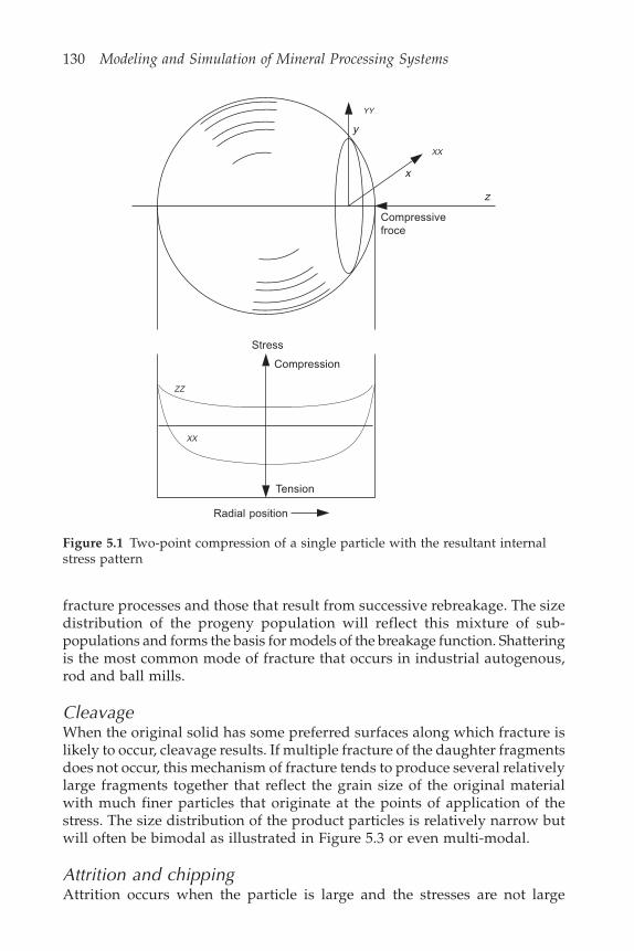
130 Modeling and Simulation of Mineral Processing Systems
fracture processes and those that result from successive rebreakage. The sizedistribution of the progeny population will reflect this mixture of sub-populations and forms the basis for models of the breakage function. Shatteringis the most common mode of fracture that occurs in industrial autogenous,rod and ball mills.
CleavageWhen the original solid has some preferred surfaces along which fracture islikely to occur, cleavage results. If multiple fracture of the daughter fragmentsdoes not occur, this mechanism of fracture tends to produce several relativelylarge fragments together that reflect the grain size of the original materialwith much finer particles that originate at the points of application of thestress. The size distribution of the product particles is relatively narrow butwill often be bimodal as illustrated in Figure 5.3 or even multi-modal.
Attrition and chippingAttrition occurs when the particle is large and the stresses are not large
YY
y
XX
x
z
Compressivefroce
Stress
Compression
XX
ZZ
Tension
Radial position
Figure 5.1 Two-point compression of a single particle with the resultant internalstress pattern
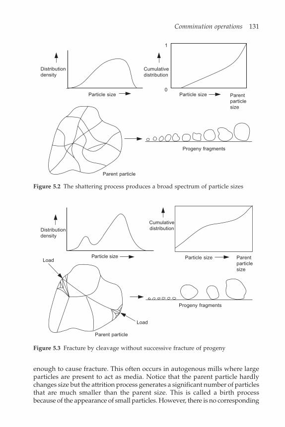
Comminution operations 131
enough to cause fracture. This often occurs in autogenous mills where largeparticles are present to act as media. Notice that the parent particle hardlychanges size but the attrition process generates a significant number of particlesthat are much smaller than the parent size. This is called a birth processbecause of the appearance of small particles. However, there is no corresponding
Figure 5.2 The shattering process produces a broad spectrum of particle sizes
Particle size
Distributiondensity
Load
Load
Parent particle
Progeny fragments
Particle size Parentparticlesize
Cumulativedistribution
Figure 5.3 Fracture by cleavage without successive fracture of progeny
Partical size
Distributiondensity
Cumulativedistribution
0Particle size Parent
particlesize
Progeny fragments
Parent particle
1
Particle size
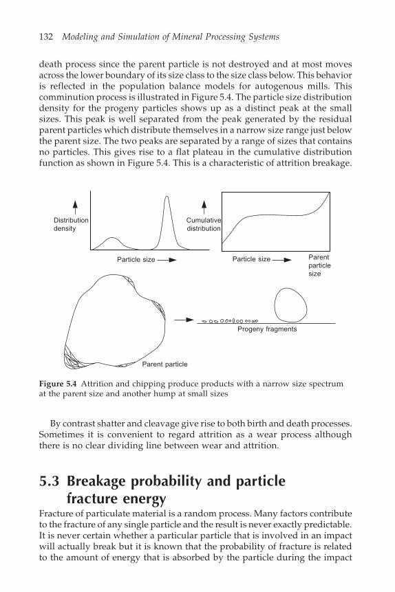
132 Modeling and Simulation of Mineral Processing Systems
death process since the parent particle is not destroyed and at most movesacross the lower boundary of its size class to the size class below. This behavioris reflected in the population balance models for autogenous mills. Thiscomminution process is illustrated in Figure 5.4. The particle size distributiondensity for the progeny particles shows up as a distinct peak at the smallsizes. This peak is well separated from the peak generated by the residualparent particles which distribute themselves in a narrow size range just belowthe parent size. The two peaks are separated by a range of sizes that containsno particles. This gives rise to a flat plateau in the cumulative distributionfunction as shown in Figure 5.4. This is a characteristic of attrition breakage.
Distributiondensity
Particle size
Cumulativedistribution
Particle size Parentparticlesize
Progeny fragments
Parent particle
Figure 5.4 Attrition and chipping produce products with a narrow size spectrumat the parent size and another hump at small sizes
By contrast shatter and cleavage give rise to both birth and death processes.Sometimes it is convenient to regard attrition as a wear process althoughthere is no clear dividing line between wear and attrition.
5.3 Breakage probability and particlefracture energy
Fracture of particulate material is a random process. Many factors contributeto the fracture of any single particle and the result is never exactly predictable.It is never certain whether a particular particle that is involved in an impactwill actually break but it is known that the probability of fracture is relatedto the amount of energy that is absorbed by the particle during the impact
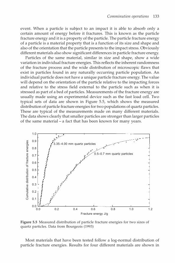
Comminution operations 133
event. When a particle is subject to an impact it is able to absorb only acertain amount of energy before it fractures. This is known as the particlefracture energy and it is a property of the particle. The particle fracture energyof a particle is a material property that is a function of its size and shape andalso of the orientation that the particle presents to the impact stress. Obviouslydifferent materials also show significant differences in particle fracture energy.
Particles of the same material, similar in size and shape, show a widevariation in individual fracture energies. This reflects the inherent randomnessof the fracture process and the wide distribution of microscopic flaws thatexist in particles found in any naturally occurring particle population. Anindividual particle does not have a unique particle fracture energy. The valuewill depend on the orientation of the particle relative to the impacting forcesand relative to the stress field external to the particle such as when it isstressed as part of a bed of particles. Measurements of the fracture energy areusually made using an experimental device such as the fast load cell. Twotypical sets of data are shown in Figure 5.5, which shows the measureddistribution of particle fracture energies for two populations of quartz particles.These are typical of the measurements made on many different materials.The data shows clearly that smaller particles are stronger than larger particlesof the same material – a fact that has been known for many years.
1.0
0.9
0.8
0.7
0.6
0.5
0.4
0.3
0.2
0.1
0.0
Cum
ulat
ive
dist
ribut
ion
of f
ract
ure
ener
gies 3.35–4.00 mm quartz particles
0.5–0.7 mm quartz particles
0.0 0.2 0.4 0.6 0.8 1.0 1.2
Fracture energy J/g
Figure 5.5 Measured distribution of particle fracture energies for two sizes ofquartz particles. Data from Bourgeois (1993)
Most materials that have been tested follow a log-normal distribution ofparticle fracture energies. Results for four different materials are shown in

134 Modeling and Simulation of Mineral Processing Systems
Figure 5.6 and the variation in the strength of the different materials isimmediately obvious. The data in this figure are plotted in the log-normalcoordinate system which produces straight lines when the data are log-normallydistributed. The data presented in Figure 5.5 also show the strong linearcharacteristic when plotted in the log-normal coordinate system.
The fracture energy is not only a function of the material and of the particlesize but it also reflects the presence of flaws in the material. Flaws in thematerial prior to impact are referred to as material damage and they aregenerated during the many natural and artificial processes that influence theparticles before they are impacted and broken in a comminution machine.The role that flaws play in particle fracture is described by the Griffith theoryof brittle fracture. When a particle is subject to rapid impact stress it initiallydeforms elastically absorbing impact energy from the impacting devices asstored elastic strain. The internal stresses in the particle increase until thestress intensity at the most sensitive flaw exceeds the Griffith criterion forunstable crack growth. A period of exceedingly rapid crack growth followswith the crack tip accelerating and often bifurcating as well. The energy thatdrives the growing crack comes from the stored elastic strain energy in theparticle, which is available to the growing crack at the requisite high rate.The crack continues to grow until it intersects the edge of the particle atwhich time the particle is fractured. Any remaining elastic stored energy isdissipated as kinetic energy of the progeny, which may suffer further fractureas a result. This model of particle fracture provides a clear explanation of theparticle fracture energy and the role that it plays in the fracture process. It isthe energy that is stored as elastic strain up to the instant of first fracture andthis represents the minimum energy that must be supplied to the particlebefore fracture will occur.
In general no one particle will absorb all of the energy that is available inany one impact event and the residual energy that remains after a particlebreaks will be available to break progeny particles in the manner describedabove. This model of particulate fracture suggests that it is the ratio of impactenergy to particle fracture energy that will determine the size distribution ofthe progeny that are produced as a result of a single impact event.
The distribution of fracture energies has another interesting interpretation.The cumulative distribution function also gives the probability that a specificparticle will fracture if it receives a given amount of energy during an impact.This follows from the fact that a particle will not break if it is impacted withless than its fracture energy. Consider a representative sample of say 100particles of quartz in the size range 0.5–0.7 mm. If each of these particles issubjected to an impact of say, 0.5 J/g the data shown in Figure 5.5 indicatethat about 35 of the particles will not break because they have particle fractureenergies greater than 0.5 J/g. Thus the probability of breakage for these particlesis 65% at an impact energy of 0.5 J/g. The same argument can be made forany other impact energy. Thus the curve in Figure 5.5 has two equally validinterpretations. On the one hand it represents the cumulative distribution of

Comminution operations 135
particle fracture energies and on the other it represents the breakage probabilityof an individual particle as a function of impact energy.
The straight lines in Figure 5.6 show that the data are well represented bythe log-normal distribution and the breakage probability of a particle thatsuffers an impact of E J/kg is given by
P E d GE E
pE
( ; ) = ln( / )50
(5.7)
99.0
97.0
90.0
70.0
50.0
30.0
10.0
3.0
1.010 100 1000
Specific particle fracture energy J/kg
Taconite
Quartz
SphaleriteGalena
Cum
ulat
ive
dist
ribut
ion
%
Figure 5.6 Cumulative distribution of particle fracture energies for different materialsmeasured in single-particle fracture tests. The data are plotted in the log-normalcoordinate system (Tavares and King, 1998)
with
G x e dtx
t( ) = 12 –
– /22(5.8)
E50 is the median fracture energy, which varies with particle size according to
E Ed
d dp p50
0
min = 1 +
–(5.9)
Values of the parameters d0 and are material specific and have been measuredfor several common minerals and these are shown in Table 5.1. dp min is thelower limit of brittle fracture. Particles smaller than dp min are deformed during

136 Modeling and Simulation of Mineral Processing Systems
impact and do not fracture. This limit is about 0.3 m for quartz. E is themedian particle fracture energy for large particles, usually about 1 cm ormore.
Table 5.1 Parameters that relate the mean mass-specific particle fracture energy toparticle size for some common minerals. From Tavares and King (1998)
Material E J/kg dp0 mm Size range, mm
Apatite 1.05 19.3 1.62 0.25–8.00Galena 3.19 7.31 1.03 0.70–7.60Gilsonite 5.50 7.03 1.60 1.18–10.0Quartz 43.4 3.48 1.61 0.25–4.75Sphalerite 7.00 8.24 1.16 0.35–10.0Magnetite 9.56 3.93 1.96 0.25–7.20Copper ore 96.1 1.17 1.26 0.25–15.8Iron ore 47.3 1.08 2.30 0.25–15.0Limestone 114.2 0.490 2.05 0.35–5.60Marble 45.9 0.882 2.66 0.50–15.0Taconite 235.9 0.803 1.42 0.35–6.00Taconite 163.3 0.856 1.76 0.35–10.0
Equation 5.9 reflects the fact that the measured median particle fracture energyis independent of particle size for particles larger than a few millimeters, butincreases quite sharply as the particle size decreases below approximately1 mm.
5.4 Progeny size distribution when a singleparticle breaks – the breakage function
It is clear that the breakage of a single particle will produce an entire spectrumof progeny sizes. When dealing with comminution processes, the distributionof breakage product sizes must be considered on a number of levels.
(a) Breakage of a specific single particle only once generating a few daughterfragments. (This is referred to as single-particle primary fracture orcleavage).
(b) Breakage of a single particle followed by sequential breakage of someof the progeny during a single breakage event. This is referred to assingle-particle, single-event fracture. All the impact energy is dissipatedin a single impact event. Some of the energy is consumed by the fractureof the parent particle and by some members of successive generationsof the progeny, some is absorbed by progeny particles without fractureand the remainder is dissipated by steel-on-steel impact. A single-impact event has total duration of a few milliseconds and the successive
Comminution operations 137
progeny breakage events follow each other at intervals of a few tens ofmicroseconds.
(c) The breakage of many single particles all of the same size in single-particle, single-impact events that produces statistically many daughterfragments. In other words repeated events of type (b).
(d) The breakage of many particles and the immediately succeeding progenyduring a single impact on a bed of particles. Particles in the bed suffersingle-particle, single-event impact each one using only a fraction ofthe total impact energy that is available for the event. This is referredto as a particle-bed single-impact event.
(e) Concurrent breakage of many particles in a comminution machine byparticle-bed single impact events. The progeny from these eventsimmediately become available for fracture in later impact events.
Each of these conceptual situations produces a different size distribution andit is important to distinguish clearly between them. (a) is not of much interestexcept as a basic event to produce the statistically meaningful (c). The productsize distribution produced by a test of type (c) is known as the single-particlebreakage function and it can be measured in a sequence of single-particlefracture tests all starting with particles of the same size.
The single-particle breakage function is defined by B(x; y) = fraction ofdaughter particles smaller than size x that result from fracture of a singleparticle of size y as described in paragraph (c) above.
Single-particle breakage tests are easy to do in the laboratory and a numberof ingenious apparatus designs have been developed. The simplest is thedrop weight test apparatus which is illustrated in Figure 5.7. A weight, usuallyspherical, is dropped from a known height on to a single particle that issupported on a hard surface. The kinetic energy of the sphere just prior toimpact is equal to mgh where m is the mass of the drop weight. This kineticenergy is transferred to the particle, which may or may not fracture. The testis repeated many times on single particles all having the same size. Thefracture products are collected for the determination of the product sizedistribution.
In spite of the use of a single particle for each test, each fracture eventconsists of a sequence of individual breakage events. Usually the energy inthe drop weight is sufficient to cause a primary fracture to occur and theresidual energy in the drop weight is then absorbed by the daughter fragmentswhich in turn are fractured forming their own progeny. The process of breakingsuccessive generations of progeny continues until all of the energy in thedrop weight is dissipated or until all of the progeny have been expelled fromthe impact zone and the drop weight collides with the hard support surfaceand dissipates all of its remaining energy as metal deformation or as elasticrebound.
The successive breakage and rebreakage of progeny particles in the single-particle, single-impact test means that the breakage function determined fromsuch a test is itself a composite of many individual primary breakage functions
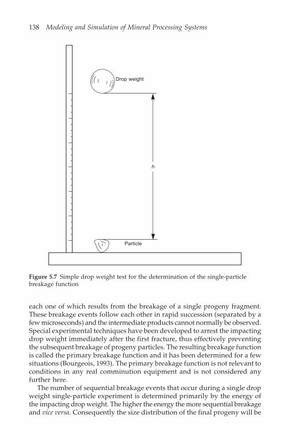
138 Modeling and Simulation of Mineral Processing Systems
each one of which results from the breakage of a single progeny fragment.These breakage events follow each other in rapid succession (separated by afew microseconds) and the intermediate products cannot normally be observed.Special experimental techniques have been developed to arrest the impactingdrop weight immediately after the first fracture, thus effectively preventingthe subsequent breakage of progeny particles. The resulting breakage functionis called the primary breakage function and it has been determined for a fewsituations (Bourgeois, 1993). The primary breakage function is not relevant toconditions in any real comminution equipment and is not considered anyfurther here.
The number of sequential breakage events that occur during a single dropweight single-particle experiment is determined primarily by the energy ofthe impacting drop weight. The higher the energy the more sequential breakageand vice versa. Consequently the size distribution of the final progeny will be
Figure 5.7 Simple drop weight test for the determination of the single-particlebreakage function
Drop weight
h
Particle
Comminution operations 139
determined to a large extent by the impact energy and to a lesser extent bythe nature of the material. A model for the single-particle breakage functionthat is based on these ideas is given below.
The breakage function plays a pivotal role in the quantitative descriptionof comminution processes. It is not the final product size distribution fromany comminution operation because the progeny particles are themselvesbroken and rebroken in many successive breakage events. In any comminutionmachine, many particles are involved in each impact event so that the single-particle breakage function that is measured in a single-particle test cannot beapplied directly to the breakage processes that occur inside the machine.Single-impact test can be conducted on particle beds and the resultant breakagefunction can be measured. It is important to distinguish among the primarybreakage event, the single-particle impact event and the single-impact particlebed event. Each kind of event is characterized by its own distinctive breakagefunction. It is only the single-impact particle-bed event that is directly relevantto conditions inside a grinding mill.
A single impact on a bed of particles is regarded as the elementary breakageevent that occurs in a grinding mill. Such an event itself consists of manysubevents such as the capture of energy by individual particles and the fractureof parent particles and the subsequent immediate rebreakage of some of theirprogeny. It is the combination of the results of all of these subevents thatconstitute the elementary breakage event. It is only the result of all the subeventstogether that can be observed because the subevents occur too quickly andcannot be distinguished. The total event typically lasts no more than a fewmilliseconds.
5.4.1 Empirical models for the breakage function thatare based on mixtures of progeny populations
Mixtures of populations with logarithmic distributionsThere have been many attempts to determine the form of the function B(x; y)for each kind of breakage event on theoretical grounds but no reliable theoreticalmodel has been found that will reproduce the size distribution that is producedin single-impact fracture tests. However some empirical models have beenfound to provide good descriptions of the experimental data.
The most popular of these models is based on the idea that the progenypopulation is made up of a mixture of two separate populations as illustratedin Figures 5.3 and 5.4. Each has a cumulative distribution that can be modeledby
B x yxy
n
( ; ) is proportional to (5.10)
Different values of n describe the larger products produced by tensile stressand the smaller products produced by the intense compressive stress at the

140 Modeling and Simulation of Mineral Processing Systems
points of application. The two distributions are added using an appropriatefractional weighting factor.
B x y Kxy
Kxy
n n
( ; ) = + (1 – )1 2
(5.11)
The first term in Equation 5.11 describes the size distribution of the finefraction in the population of progeny particles and K is the fraction of daughterproducts that contribute to the finer fraction.
The geometry of this function provides an insight into the role that eachparameter plays and also provides a convenient method for the estimation ofthe parameters K, n1 and n2 when experimental data is available for thebreakage function. The data is plotted on log-log coordinates as shown inFigure 5.9. If n2 > n1 then
xy
xy
xy
n n1 2
> as 0 (5.12)
100
10–1
10–2
654
3
2
654
3
2
10–2 2 3 4 5 10–1 2 3 4 5 100
(a) – (b)Slope = n2
(b)
(a)
Bre
akag
e fu
nctio
n B
(x;
y )
Slope = n1
Intercept = 1 – K
Intercept = K
x/y
Figure 5.8 A typical breakage function showing the procedure for evaluation of theparameters k, n1 and n2
Then at low values of xy
B x y Kxy
n
( ; ) = 1
(5.13)
Comminution operations 141
which plots as a straight line with slope n1 on the log-log coordinates asshown in Figure 5.8. The straight line will intersect the ordinate x/y = 1 at thepoint B(x; y) = K as shown. Thus the parameters n1 and K can be establishedeasily by drawing the tangent from the lower left of the curve and readingthe intercept at x/y = 1. Once this line has been established, the difference
B x y Kxy
Kxy
n n
( ; ) – = (1 – )1 2
(5.14)
can be plotted as shown in the figure. This will produce another straight lineof slope n2 and intercept (1 – K) at x/y = 1. The value of n2 can be determinedfrom the slope of this line.
It sometimes happens that the difference between the original curve (a)and the first straight line (b) is itself a curve rather than a straight line. Sucha curve can be resolved into two terms using the same procedure and theentire function B(x; y) will then consist of three power function terms.
The breakage function described by Equation 5.11 is independent of thesize of the parent particle and depends only on the ratio x/y. The samefunction can be used for all parent sizes and the distribution is said to benormalized with respect to the parent size.
If the experimental data do not normalize, the fraction K must be determined
Figure 5.9 Non-normalized breakage function showing the effect of variations in theparent size
100
10–1
10–2
10–2 10–1 1004 7 2 5 7
Parent particle size = 1 mmParent particle size = 0.4 mmParent particle size = 0.2 mmParent particle size = 0.1 mm
Bre
akag
e fu
nctio
n
Relative particle size
142 Modeling and Simulation of Mineral Processing Systems
as a function of the parent size. This is illustrated in Figure 5.9. Usually thiseffect is modeled using a simple inverse power function
K y Kyy
( ) = 00 (5.15)
where y0 is a reference parent size usually taken to be 5 mm.As the parent particles become too large to be properly nipped between
the media particles, the breakage function becomes bimodal reflecting thegreater tendency of the particles to chip rather than to shatter. Under thesecircumstances the breakage function becomes bimodal as shown in Figure5.10.
Figure 5.10 Experimentally determined breakage functions for parent particles ofdifferent size. 26.6 mm diameter balls were used. The distribution is distinctly bi-modal at larger particle sizes. Data from Austin et al. (1987)
Parent particle size
12.7 9.52 mm9.52 6.35 mm4.75 3.35 mm1.18 0.85 mm
100
10–1
10–2
10–2 10–1 100
Relative progeny size X/Y
Bre
akag
e fu
nctio
n B
(x;
y )
This behavior can be modeled approximately in the following way.
B x y Kxy
xy
Kxy
x yn n n
( ; ) = + (1 – ) for < 0
0
3 1 2
(5.16)
and

Comminution operations 143
B x y Kxy
Kxy
x yn n
( ; ) = + (1 – ) for 1 2
0 (5.17)
y0 is the largest chip size which must obviously be smaller than the parentsize y.
The four parameters K, n1, n2, and n3 are functions of the impact energybut the exact dependence has never been systematically investigated. Theycan also vary with ball size in a ball mill and a weighted average breakagefunction can be used to increase the accuracy of calculation.
Models for the breakage function that are based ontruncated standard distributionsAny of the truncated distributions that are described in Section 2.2.2 areuseful models for the breakage function. Typical representations of the truncatedRosin-Rammler, truncated logistic and truncated log-normal distributionsare shown in Figure 5.11.
Measurements indicate that the truncated distributions are not alwaysflexible enough to describe the breakage behavior under all conditions, for
Figure 5.11 Some typical representations of the breakage function using standardtruncated distribution functions
100
10–1
10–2
10–2 10–1 100
Truncated logistic distribution
Truncated log-normal distribution
Truncated Rosin-Rammler distribution
Progeny size/Parent size
Bre
akag
e fu
nctio
n
144 Modeling and Simulation of Mineral Processing Systems
example during slow compression of constrained beds and the size distributionsmeasured in single particle breakage tests have been correlated assumingthat the progeny are made up from several populations each of which has atruncated log-normal size distribution.
B x y E E F x yn
N
n n( ; , ) = ( ) ( , )=1
(5.18)
where the functions Fn(x, y) are truncated log-normal distributions given by
F x y G
x x x
x x xn
n n
n n
n( , ) =
ln( –
( – )0( )
50( )
50( )
0( )
( )(5.19)
and G is the normal distribution function defined by
G x t dtx
( ) = 12
exp(– /2)–
2 (5.20)
and x n0( ) is the upper truncation size for the nth population. The coefficients
n(E) are the weighting fractions for the separate distributions and thesedepend quite strongly on the impact energy. The parameters x xn n
0( )
50( ), and
(n) of Equation 5.19 are largely insensitive to the impact energy but dependon the parent size y. In Equation 5.19, Fn(x, y) is defined to be 1 wheneverx x n .0
( ) See Dan and Schubert (1990).
5.4.2 Models for the breakage function that arebased on the impact energy
Single-impact tests have shown clearly that the breakage function is determinedprimarily by the amount of energy that is available to break the materialduring the impact. The larger the amount of energy in the impact, the finerthe progeny that result from that impact. This is due largely to the successivebreakage and rebreakage of the progeny until the total impact energy isdissipated. Data from a series of single-particle, single-impact tests at differentimpact energies are shown in Figure 5.12. The data are plotted using a relativesize scale n = (parent size/progeny size). The effect of the increasing impactenergy is apparent in the data. It is postulated that the same relationshipbetween breakage function and energy will be obtained when the impactinvolves a bed of particles. In that case however the progeny that resultsfrom any one particle in the bed will be governed by the fraction of the totalimpact energy that is absorbed by that particle. The breakage function thatresults from the impact as a whole is the sum total of all the individualbreakage functions from each particle that absorbs enough energy to break.
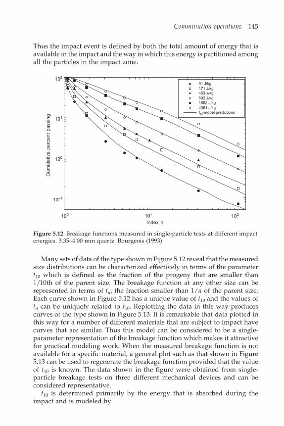
Comminution operations 145
Thus the impact event is defined by both the total amount of energy that isavailable in the impact and the way in which this energy is partitioned amongall the particles in the impact zone.
102
101
100
10–1
100 101 102
Index n
Cum
ulat
ive
perc
ent
pass
ing
Figure 5.12 Breakage functions measured in single-particle tests at different impactenergies. 3.35–4.00 mm quartz. Bourgeois (1993)
Many sets of data of the type shown in Figure 5.12 reveal that the measuredsize distributions can be characterized effectively in terms of the parametert10 which is defined as the fraction of the progeny that are smaller than1/10th of the parent size. The breakage function at any other size can berepresented in terms of tn, the fraction smaller than 1/n of the parent size.Each curve shown in Figure 5.12 has a unique value of t10 and the values oftn can be uniquely related to t10. Replotting the data in this way producescurves of the type shown in Figure 5.13. It is remarkable that data plotted inthis way for a number of different materials that are subject to impact havecurves that are similar. Thus this model can be considered to be a single-parameter representation of the breakage function which makes it attractivefor practical modeling work. When the measured breakage function is notavailable for a specific material, a general plot such as that shown in Figure5.13 can be used to regenerate the breakage function provided that the valueof t10 is known. The data shown in the figure were obtained from single-particle breakage tests on three different mechanical devices and can beconsidered representative.
t10 is determined primarily by the energy that is absorbed during theimpact and is modeled by
91 J/kg171 J/kg463 J/kg692 J/kg1652 J/kg4361 J/kgt10-model predictions
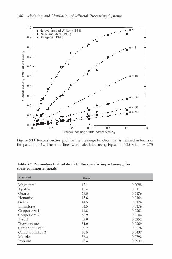
146 Modeling and Simulation of Mineral Processing Systems
Narayanan and Whiten (1983)Pauw and Mare (1988)Bourgeois (1993)
1.0
0.9
0.8
0.7
0.6
0.5
0.4
0.3
0.2
0.1
0.0
n = 2
n = 4
n = 10
n = 25
n = 50
n = 75
0.0 0.1 0.2 0.3 0.4 0.5 0.6Fraction passing 1/10th parent size-t10
Fra
ctio
n pa
ssin
g 1/
nth
par
ent
size
- tn
Figure 5.13 Reconstruction plot for the breakage function that is defined in terms ofthe parameter t10. The solid lines were calculated using Equation 5.25 with = 0.75
Table 5.2 Parameters that relate t10 to the specific impact energy forsome common minerals
Material t10max
Magnetite 47.1 0.0098Apatite 45.4 0.0115Quartz 38.8 0.0176Hematite 45.6 0.0164Galena 44.5 0.0176Limestone 54.5 0.0176Copper ore 1 44.8 0.0263Copper ore 2 58.9 0.0204Basalt 52.0 0.0252Titanium ore 51.0 0.0269Cement clinker 1 69.2 0.0276Cement clinker 2 60.5 0.0437Marble 76.3 0.0792Iron ore 65.4 0.0932
Comminution operations 147
t t e E E10 10max
– / = (1 – )50 (5.21)
The parameters t10max and are material specific and they can be determinedeasily in the laboratory using standard drop weight apparatus. The test canbe performed on single particles or on beds of particles. Values for somecommon minerals are given in Table 5.2.
The entire breakage function can be regenerated from the single value oft10 using a reconstruction plot such as that shown in Figure 5.13. A number ofmodels have been investigated to provide a suitable structure for the behaviorshown in Figure 5.13. Models based on the standard truncated distributionfunctions are particularly useful because they are characterized in terms ofonly one or two parameters and these are described in the next section.
The t10 model based on truncated distribution functionsThe truncated Rosin-Rammler distribution is given by Equation 2.18.
P D D dp( ) = 1 – exp – for 63.2
(5.22)
with
= 1 –
and = Ddp
From the definition of t10
t Pdp
1063.2
= 10
= 1 – exp – 1(10 – 1)
(5.23)
and from the definition of tn
t Pdn nnp
= = 1 – exp – 1( – 1) 63.2
(5.24)
When 63.2 is eliminated from these two equations
t tnn = 1 – (1 – )10
10–1–1 (5.25)
which shows the unique relationship between tn and t10. The parameter ismaterial specific but representative values for different materials have notyet been investigated.
Similar manipulations give the following relationships for the truncatedlogistic and truncated log-normal distributions respectively.
tt
tn
n = 1
1 + 1 – – 1
910
10
(5.26)
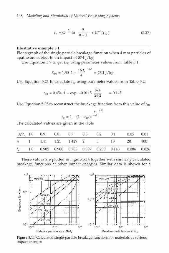
148 Modeling and Simulation of Mineral Processing Systems
t Gn
G tn = 1 ln 9– 1
+ ( )–110 (5.27)
Illustrative example 5.1Plot a graph of the single-particle breakage function when 4 mm particles ofapatite are subject to an impact of 874 J/kg.
Use Equation 5.9 to get E50 using parameter values from Table 5.1.
E50
1.62 = 1.50 1 + 19.3
4 = 26.1 J/kg
Use Equation 5.21 to calculate t10 using parameter values from Table 5.2.
t10 = 0.454 1 – exp –0.011587426.2
= 0.145
Use Equation 5.25 to reconstruct the breakage function from this value of t10.
t tnn = 1 – (1 – )10
9–1
0.75
The calculated values are given in the table
D dp/ 1.0 0.9 0.8 0.7 0.5 0.2 0.1 0.05 0.01
n 1 1.11 1.25 1.429 2 5 10 20 100
tn 1.0 0.985 0.900 0.785 0.557 0.250 0.145 0.086 0.026
These values are plotted in Figure 5.14 together with similarly calculatedbreakage functions at other impact energies. Similar data is shown for a
Figure 5.14 Calculated single-particle breakage functions for materials at variousimpact energies
100
10–1
10–2
Bre
akag
e fu
nctio
n
10–2 10–1 100
Relative particle size D d p/
100
10–1
10–2
10–2 10–1 100
Relative particle size D d p/
Apatite
6488 J/kg
1504 J/kg
254 J/kg
Iron ore
6488 J/kg
874 J/kg
1504 J/kg
254 J/kg
874 J/kg
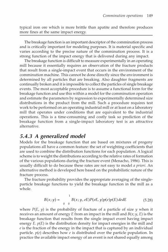
Comminution operations 149
typical iron ore which is more brittle than apatite and therefore producesmore fines at the same impact energy.
The breakage function is an important descriptor of the comminution processand is critically important for modeling purposes. It is material specific andvaries according to the precise nature of the comminution process. It is astrong function of the impact energy that is delivered during any impact.
The breakage function is difficult to measure experimentally in an operatingmill because it essentially requires an observation of the fracture productsthat result from a single-impact event that occurs in the environment of thecomminution machine. This cannot be done directly since the environment isdetermined by all particles that are breaking. Also daughter fragments arecontinually broken and it is impossible to collect the particles of single breakageevents. The most acceptable procedure is to assume a functional form for thebreakage function and use this within a model for the comminution operationand estimate the parameters by regression to experimentally determined sizedistributions in the product from the mill. Such a procedure requires testwork to be performed on an operating industrial mill or at least on a laboratorymill that operates under conditions that are equivalent to the industrialoperations. This is a time-consuming and costly task so prediction of thebreakage function from a single-impact laboratory test is an attractivealternative.
5.4.3 A generalized modelModels for the breakage function that are based on mixtures of progenypopulations all have a common feature: the set of weighting coefficients thatare used to combine the distribution functions for each population. A logicalscheme is to weight the distributions according to the relative rates of formationof the various populations during the fracture event (Menacho, 1986). This isusually difficult to do because these rates are not easy to model a priori. Analternative method is developed here based on the probabilistic nature of thefracture process.
The fracture probability provides the appropriate averaging of the single-particle breakage functions to yield the breakage function in the mill as awhole.
B x y B x y eE P eE, y p e p E dedE( ; ) = ( ; , ) ( ) ( ) ( )0
1
0(5.28)
where P(E, y) is the probability of fracture of a particle of size y when itreceives an amount of energy E from an impact in the mill and B(x; y, E) is thebreakage function that results from the single impact event having impactenergy E. p(E) is the distribution density for impact energies in the mill ande is the fraction of the energy in the impact that is captured by an individualparticle. p(e) describes how e is distributed over the particle population. Inpractice the available impact energy of an event is not shared equally among
150 Modeling and Simulation of Mineral Processing Systems
all particles that are involved with the event. Consequently the availableimpact energy is shared among the particles. The fraction of the availableenergy that a particular particle captures during the event is primarily afunction of the position that the particle occupies relative to the impact axisamong those particles that are in the impact zone. Particles that are on orclose to the impact axis are likely to capture more of the available energy thanparticles that are off the axis. Larger particles tend to capture more of theenergy than smaller particles. There will be considerable rearrangement ofparticles in the bed during the course of a single impact. At present little isknown about these processes. p(E) is the distribution density for impact energiesin the mill as a whole and it has been extensively investigated in recent yearsusing the discrete element method (Rajamani et al., 1995). Equation 5.28 providesa link between single-particle fracture tests and the behavior of the materialin an operating mill.
5.5 Energy requirements for comminutionObviously it takes energy to fracture a particle. The energy absorbed bysingle-particle fracture is a random variable. Each particle will require a differentamount of energy depending on the distribution of flaw sizes and on thefracture process (rate of stress application, orientation of particle in the stressfield etc.).
Single-particle impact fracture data show that greater amounts of energyabsorbed by the particle leads to finer average size of the product population.This leads to the concept of energy absorption by a particle population andthe continuing absorption of energy as the size distribution shifts to finer andfiner sizes.
A rough empirical expression for energy absorption during comminutioncan be obtained by following some representative size of the particle populationas it steadily decreases with the amount of comminution energy that is putinto the particulate material.
Let dr be a representative size. It could be the mean size on either a number-weighted or mass-weighted basis, but is often the 80% passing size (massbasis). There is nothing magical about the choice of representative size but itis important to maintain consistency once a choice has been made.
The relationship between comminution energy absorbed per unit massand the representative size is defined by a differential equation:
dEdd
f dr
r = ( ) (5.29)
f (dr) is a decreasing function of dr reflecting the fact that more energy per unitmass is required as the particles get smaller.
A variety of formulations for the functional form of f (dr) have been proposedand the three most common approaches are ascribed to Kick (1883), Rittinger(1857) and Bond (1952). Each of these suggest a functional form of the type

Comminution operations 151
f d Kdr rn( ) = – – (5.30)
with n having the valuen = 1 (Kick)n = 1.5 (Bond)n = 2 (Rittinger)
A value of n greater than 1 reflects an increase in energy per unit massfractured as the particle size decreases.
The energy equation can be integrated from the initial condition that E =0 when dr = drI for the parent population
dEdd
Kdr
rn = – –
E Kn
d C n
Kn
d C
rn
rn
= –1 –
+ 1
0 = –1 –
+
(1– )
(1– )1
(5.31)
E Kn d dr
n–r
nI
= – 1
1 – 1( 1) ( –1)
when n = 1 Kick
E Kdd
r
r
I = ln (5.32)
when n = 1.5 Bond
E Kd dr rI
= 2 1 – 11/2 1/2
(5.33)
when n = 2 Rittinger
E Kd dr rI
= 1
–1
(5.34)
These equations can be given approximate physical interpretations:In the case of Kick’s law energy consumed is proportional to the size
reduction ratio, i.e. it takes the same amount of energy to reduce a populationof particles from a representative size of 100 cm to a representative size of1 cm as it takes to reduce from 1 mm to 10 microns.
In the case of Rittinger’s law, the reciprocal of representative size can beregarded as being proportional to the average surface area per unit volumein the particle population. Thus energy consumed is proportional to the increasein surface area per unit volume.
This simple analysis forms the basis of the use of the Bond work index toassess energy requirements for rod and ball milling. This method is describedin Section 5.15.1.
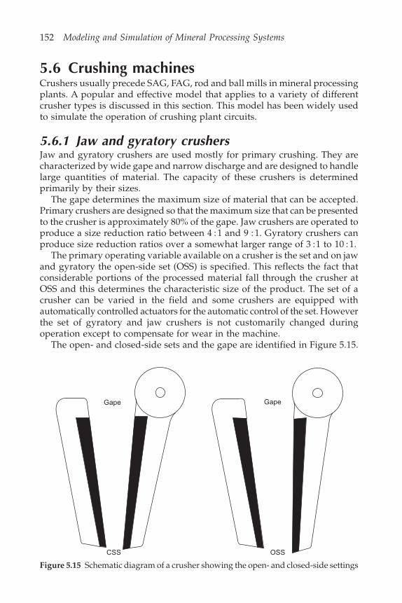
152 Modeling and Simulation of Mineral Processing Systems
5.6 Crushing machinesCrushers usually precede SAG, FAG, rod and ball mills in mineral processingplants. A popular and effective model that applies to a variety of differentcrusher types is discussed in this section. This model has been widely usedto simulate the operation of crushing plant circuits.
5.6.1 Jaw and gyratory crushersJaw and gyratory crushers are used mostly for primary crushing. They arecharacterized by wide gape and narrow discharge and are designed to handlelarge quantities of material. The capacity of these crushers is determinedprimarily by their sizes.
The gape determines the maximum size of material that can be accepted.Primary crushers are designed so that the maximum size that can be presentedto the crusher is approximately 80% of the gape. Jaw crushers are operated toproduce a size reduction ratio between 4 :1 and 9 : 1. Gyratory crushers canproduce size reduction ratios over a somewhat larger range of 3 :1 to 10 :1.
The primary operating variable available on a crusher is the set and on jawand gyratory the open-side set (OSS) is specified. This reflects the fact thatconsiderable portions of the processed material fall through the crusher atOSS and this determines the characteristic size of the product. The set of acrusher can be varied in the field and some crushers are equipped withautomatically controlled actuators for the automatic control of the set. Howeverthe set of gyratory and jaw crushers is not customarily changed duringoperation except to compensate for wear in the machine.
The open- and closed-side sets and the gape are identified in Figure 5.15.
Figure 5.15 Schematic diagram of a crusher showing the open- and closed-side settings
Gape
CSS
Gape
OSS
Comminution operations 153
Table 5.3 Characteristics that determine the product type
Crusher work index, Material characteristic Product type, PTkW hr/tonne
5–10 Soft 90Soft spongy 85
10–13 Average 90Average spongy 85
>13 Hard brittle 90Hard tough 82Hard slabby 75
The throw of the crusher is the distance that moving jaw moves in goingfrom OSS to CSS.
Throw = OSS – CSS.
The capacity is a function of size and OSS. Manufacturers publish tables ofcapacity for their crushers of various size as a function of the open-side set.
Product size distributions in gyratory and jaw crusher productsPrimary crushers usually receive feed that contains only small amounts ofmaterial that is smaller than the open-side set of the crusher. Thus almost allof the feed material is crushed in the machine.
The size distribution of the material in the product is independent of thesize distribution in the feed and is a function primarily of the setting of thecrusher and to a lesser extent of the nature of the material that is crushed.Product size distributions are often of Rosin-Rammler type with the parametersof the distribution varying with the product particle size.
The size distribution of the product is characterized by the size relative tothe open-side setting
rD
OSSii = (5.35)
and to the ‘product type’ PT which is specified in terms of the fraction of theproduct that is smaller than the open-side setting. This parameter is relatedto the nature of the material, as shown in Table 5.3.
Two derived parameters are derived from PT as follows:
KPU
T = ln
11 –
–0.67
(5.36)
and
154 Modeling and Simulation of Mineral Processing Systems
KPL
b = 0.5 ln
11 –
–1.18
(5.37)
with
PKb
U = 1 – exp –
0.5 1.5
(5.38)
The size distribution is given by
P Dr
Kr
rK
r
U
L
( ) = 1 – exp – for > 0.5
= 1 – exp – for 0.5
1.5
0.85(5.39)
These equations can lead to inconsistent results since they take no account ofthe distribution of particle sizes in the feed to the crusher and should beapplied only when the open-side setting of the crusher is smaller than the d50size in the feed.
The model that is described above is based on data from a single crushermanufacturer and is probably specific to the machine design. An alternatemodel that has been reported to describe the distribution of particle sizes inthe product from gyratory crushers is the simple normalized logarithmicdistribution
P Dr
ri( ) = 1.25
for 1.250.843
(5.40)
5.6.2 Cone crushersCone crushers are commonly used for secondary, tertiary and quaternarycrushing duties. Two variations of cone crusher are used – standard andshort head. The chief difference between cone and gyratory or jaw crushersis the nearly parallel arrangement of the mantle and the cone at the dischargeend of the cone crusher. This is illustrated in Figure 5.16. Reduction ratios inthe following ranges are common for cone crushers: 6 :1 – 8 : 1 for secondariesand 4 : 1–6 :1 for tertiary and quaternary crushing.
The size distribution of the products tends to be determined primarily bythe CSS since no particle can fall through during a single open-side periodand all particles will experience at least one closed-side nip during passagethrough the crusher. The CSS is adjusted by screwing the bowl of the crusherup or down. It is not unusual for cone crushers to be fitted with hydrauliccontrols so that the setting on the crusher can be changed during operationwith relative ease and as part of an automatic control loop if necessary.
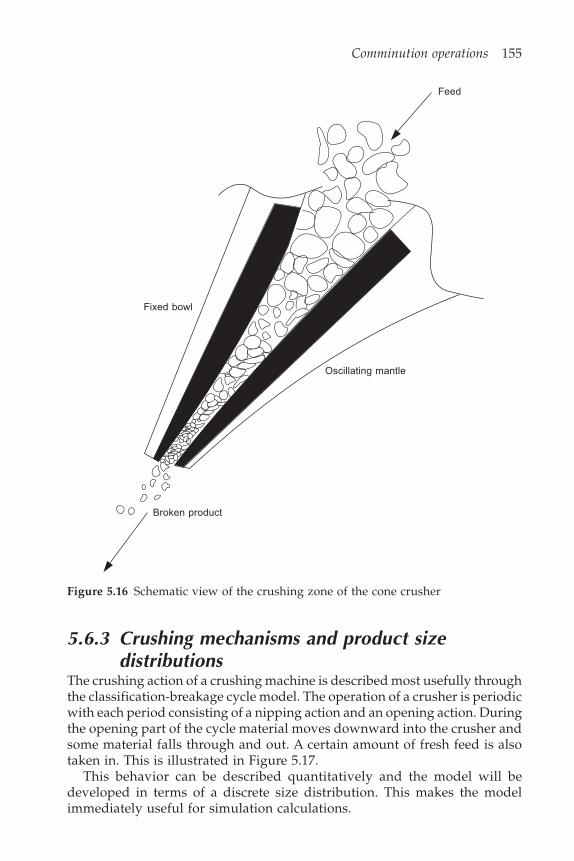
Comminution operations 155
5.6.3 Crushing mechanisms and product sizedistributions
The crushing action of a crushing machine is described most usefully throughthe classification-breakage cycle model. The operation of a crusher is periodicwith each period consisting of a nipping action and an opening action. Duringthe opening part of the cycle material moves downward into the crusher andsome material falls through and out. A certain amount of fresh feed is alsotaken in. This is illustrated in Figure 5.17.
This behavior can be described quantitatively and the model will bedeveloped in terms of a discrete size distribution. This makes the modelimmediately useful for simulation calculations.
Figure 5.16 Schematic view of the crushing zone of the cone crusher
Feed
Fixed bowl
Broken product
Oscillating mantle
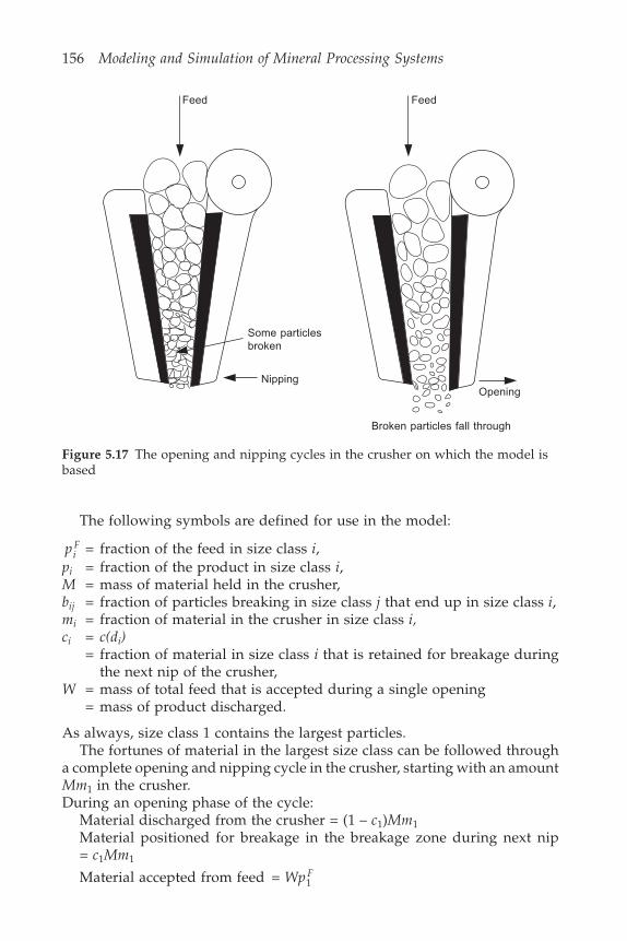
156 Modeling and Simulation of Mineral Processing Systems
The following symbols are defined for use in the model:
piF = fraction of the feed in size class i,
pi = fraction of the product in size class i,M = mass of material held in the crusher,bij = fraction of particles breaking in size class j that end up in size class i,mi = fraction of material in the crusher in size class i,ci = c(di)
= fraction of material in size class i that is retained for breakage duringthe next nip of the crusher,
W = mass of total feed that is accepted during a single opening= mass of product discharged.
As always, size class 1 contains the largest particles.The fortunes of material in the largest size class can be followed through
a complete opening and nipping cycle in the crusher, starting with an amountMm1 in the crusher.During an opening phase of the cycle:
Material discharged from the crusher = (1 – c1)Mm1Material positioned for breakage in the breakage zone during next nip= c1Mm1
Material accepted from feed = 1Wp F
Figure 5.17 The opening and nipping cycles in the crusher on which the model isbased
Feed Feed
Some particlesbroken
NippingOpening
Broken particles fall through

Comminution operations 157
After the next nip the crusher must again have an amount Mm1 in the crushingzone since the overall operation is at steady state:
Mm Wp c Mm b
MmW
pc b
F
F1 1 1 1 11
1 1
1 11
= +
= 1 –
(5.41)
Product discharged during the opening phase = Wp1 = (1 – c1)Mm1 so that
p cMm
W1 11 = (1 – ) (5.42)
which gives the fraction of size class 1 in the crusher product.Now consider the next size down:
During an opening phase of the cycle:Material discharged = (1 – c2)Mm2Material positioned for breakage during next nip = c2Mm2Material accepted from feed = 2Wp F
After next nip:
Mm Wp c Mm b c Mm b
MmW c b
p cMm
Wb
F
F
2 2 2 2 22 1 1 21
2
2 222 1
121
= + +
= 11 –
+ (5.43)
Product discharged during the opening phase which gives the fraction of thissize class in the crusher product = Wp2 = (1 – c2)Mm2
p cMm
W2 22 = (1 – ) (5.44)
The next size down can be handled in exactly the same way to give
Mm Wp c Mm b c Mm b c Mm b
MmW c b
p cMm
Wb c
MmW
b
F
F
3 3 3 3 33 2 2 32 1 1 31
3
3 333 2
232 1
131
= + + +
= 11 –
+ + (5.45)
This procedure can be continued from size to size in an obvious way.Thus for any size class i
MmW c b
p cMm
Wbi
i iiiF
j
i
jj
ij = 11 –
+ =1
–1
(5.46)
The series of Equations 5.46 can be easily solved sequentially for the groupMmi/W starting from size class number 1. The size distribution in the productcan then be calculated from
pc MmW
cc b
p cMm
Wbi
i i i
i iiiF
j
i
jj
ij = (1 – )
= 1 –
1 – +
=1
–1
(5.47)
158 Modeling and Simulation of Mineral Processing Systems
and the distribution of sizes in the product is completely determined fromthe size distribution in the feed and a knowledge of the classification andbreakage functions ci and bij. This model is completely general and for aspecific crusher reduces to the specification of the appropriate classificationand breakage functions.
The classification function is usually of the form shown schematically inFigure 5.18. d1 and d2 are parameters that are characteristic of the crusher.They are determined primarily by the setting of the crusher. Data from operatingcrusher machines indicate that both d1 and d2 are proportional to the closedside setting. d1 is the smallest size particle that can be retained in the crushingzone during the opening phase of the cycle. d2 is the largest particle that canfall through the crushing zone during the opening phase of the cycle.
Figure 5.18 A typical internal classification function for a crusher
1.0
0.9
0.8
0.7
0.6
0.5
0.4
0.3
0.2
0.1
0.0
Cla
ssifi
catio
n fu
nctio
n c
(dp)
0 d1 d2 8
Particle size dp
A useful form of the classification function is
cd dd d
d d d
d d
ipi
n
pi
pi
= 1 –––
for < <
= 0 for
2
1 21 2
1
(5.48)
= 1 for dpi d2
For both standard and short-head Symons cone crushers, the parameters arerelated to CSS as follows:
d1 = 1 CSS (5.49)
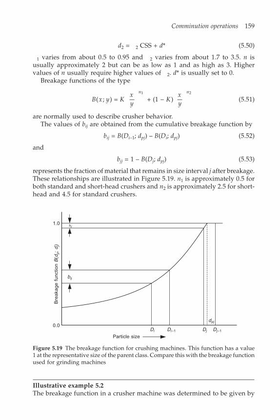
Comminution operations 159
d2 = 2 CSS + d* (5.50)
1 varies from about 0.5 to 0.95 and 2 varies from about 1.7 to 3.5. n isusually approximately 2 but can be as low as 1 and as high as 3. Highervalues of n usually require higher values of 2. d* is usually set to 0.
Breakage functions of the type
B x y Kxy
Kxy
n n
( ; ) = + (1 – )1 2
(5.51)
are normally used to describe crusher behavior.The values of bij are obtained from the cumulative breakage function by
bij = B(Di–1; dpj) – B(Di; dpj) (5.52)
and
bjj = 1 – B(Dj; dpj) (5.53)
represents the fraction of material that remains in size interval j after breakage.These relationships are illustrated in Figure 5.19. n1 is approximately 0.5 forboth standard and short-head crushers and n2 is approximately 2.5 for short-head and 4.5 for standard crushers.
1.0
0.0
Bre
akag
e fu
nctio
n B
(dp;
dj)
Particle size
Di Di –1 Dj Dj–1
dpj
bjj
bij
Figure 5.19 The breakage function for crushing machines. This function has a value1 at the representative size of the parent class. Compare this with the breakage functionused for grinding machines
Illustrative example 5.2The breakage function in a crusher machine was determined to be given by

160 Modeling and Simulation of Mineral Processing Systems
B x yxy
xy
( : ) = 0.3 + 0.70.45 3.2
If size class 2 has mesh sizes boundaries 13.4 cm and 9.5 cm and size class 5has boundaries 7.50 cm and 5.60 cm, calculate b52.
bij = B(Di–1; dpj) – B(Di; dpj)
dp 2 = 13.4 9.4 = 11.28 cm
b52
0.45 3.2 0.45 3.2
= 0.37.5
11.28 + 0.7
7.511.28
– 0.35.6
11.28– 0.7
5.611.28
= 0.4393 – 0.2934
= 0.1459
The parameters in the classification and breakage functions are obviouslyspecific to the type and size of crusher. Unfortunately not many studies havebeen done to establish their values under a range of actual operating conditionsusing predictive equations. In practice it is usual to estimate them frommeasured particle size distributions in the products from operating crushers.Once established for a particular material in a particular crusher, they remainindependent of the closed side setting. This allows the crusher performanceto be simulated as the CSS is varied.
Approximate capacities of some common crushers are given in Tables 5.4–5.7. These are average values from a number of manufacturers’ tables andshould be used only to obtain approximate values of sizes and settings forsimulation calculations.
5.7 Grinding
5.7.1 Grinding actionIndustrial grinding machines used in the mineral processing industries aremostly of the tumbling mill type. These mills exist in a variety of types – rod,ball, pebble autogenous and semi-autogenous. The grinding action is inducedby relative motion between the particles of media – the rods, balls or pebbles.This motion can be characterized as collision with breakage induced primarilyby impact or as rolling with breakage induced primarily by crushing andattrition. In autogenous grinding machines fracture of the media particlesalso occurs by both impact (self breakage) and attrition.
The relative motion of the media is determined by the tumbling actionwhich in turn is quite strongly influenced by the liners and lifters that arealways fixed inside the shell of the mill. Liners and lifters have two mainpurposes:

Comminution operations 161
Table 5.4 Approximate capacities of jaw crushers in tonnes/hr. The size designationused here is the traditional one in which the feed opening is specified as gape length in inches
Size Feed Motor Open-side setting mmopening kW
25 32 38 51 63 76 102 127 152
10 20 15 12.7 15.4 18.2 23.0 31.010 24 11 14.5 17.3 20.0 31.0 30.015 24 22 20.9 24.5 30.0 38.1 45.414 24 19 23.6 70.0 37.2 45.424 36 56 86.3 103 13630 42 75 113 136 182 227 272
Open-side setting mm
63 76 102 127 152 178 203 229 254
32 42 75 227 263 300 327 36336 48 93 189 245 300 354 40942 48 110 345 381 426 463 490 52748 60 1580 436 481 517 554 60056 72 186 454 500 567 61766 84 225 700 772 863 950
Table 5.5 Approximate capacities of gyratory crushers in tonnes/hr. Size is specifiedas gape lower mantle diameter in inches
Size Motor Open-side setting mmkW
51 63 76 89 102 114 127 140 152 178
30 60 150 313 381 450 508 567 630 695 76030 55 300 381 463 518 590 663 735 81736 60 186 458 540 604 680 755 830 900 97042 65 400 800 908 1017 1317 1500
Open-side setting mm
127 140 152 178 190 203 216 229 241 254
42 70 300 708 790 863 944 1017 109048 74 500 1544 1680 1816 1952 2088 245248 80 500 1376 1462 1562 1662 1770 187054 74 500 1634 1771 1907 2043 2180 231554 80 500 1307 1394 1490 1580 1680 177060 89 600 2270 2424 2580 2815 2960 3270
Open-side setting mm
190 203 216 229 241 254 267 279 292 305
60 102 800 2542 2760 2974 3396 3827 425460 109 800 3904 4195 4485 4776 5067 5357 5675 5993
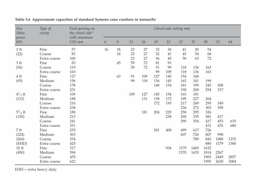
Table 5.6 Approximate capacities of standard Symons cone crushers in tonnes/hr
Size Type of Feed opening on Closed-side setting mm(Max. cavity the closed side*power with minimumkW) CSS mm 6 9 13 16 19 22 25 31 38 51 64
2 ft Fine 57 16 18 23 27 32 36 41 45 54(22) Coarse 83 18 23 27 32 41 45 54 68
Extra coarse 100 23 27 36 45 50 63 723 ft Fine 83 45 59 72 81 91(56) Coarse 119 59 72 91 99 118 136 163
Extra coarse 163 99 109 118 136 1634 ft Fine 127 63 91 109 127 140 154 168(93) Medium 156 99 118 136 145 163 181 199
Coarse 178 140 154 181 199 245 308Extra coarse 231 190 208 254 317
41/2 ft Fine 109 109 127 145 154 163 181(112) Medium 188 131 158 172 199 227 264
Coarse 216 172 195 217 249 295 349Extra coarse 238 236 272 303 358
51/2 ft Fine 188 181 204 229 258 295 326(150) Medium 213 258 290 335 381 417
Coarse 241 290 354 417 453 635Extra coarse 331 431 476 680
7 ft Fine 253 381 408 499 617 726(224) Medium 303 607 726 807 998(260) Coarse 334 789 843 1088 1270(EHD) Extra coarse 425 880 1179 138010 ft Fine 317 934 1179 1469 1632(450) Medium 394 1570 1633 1814 2267
Coarse 470 1905 2449 2857Extra coarse 622 1995 2630 3084
EHD = extra heavy duty.

Table 5.7 Approximate capacities of short head Symons cone crushers in tonnes/hr
Size Type of cavity Recommended Feed opening with Closed-side setting mm(Max. minimum CSS minimum CSS mmpower mmkW) Closed Open 3 5 6 10 13 16 19 25
side side
2 ft Fine 3 19 35 9 6 18 27 36(22) Coarse 5 38 51 16 22 29 413 ft Fine 3 13 41 27 41 54 68 91(56) Medium 3 33 60 27 41 54 68 91 99
Extra coarse 5 51 76 59 72 95 113 1274 ft Fine 5 29 57 50 77 86 122 131(93) Medium 8 44 73 91 131 145
Coarse 13 56 89 140 163 181Extra coarse 16 89 117 145 168 190 217
41/2 ft Fine 5 29 64 59 81 104 136 163(112) Medium 6 54 89 81 104 136 163
Coarse 8 70 105 109 158 181 199 227Extra coarse 13 98 133 172 190 254 238
51/2 ft Fine 5 35 70 91 136 163 208(150) Medium 6 54 89 136 163 208 254 281
Coarse 10 98 133 190 254 281 308 598Extra coarse 13 117 133 254 281 308 653
7 ft Fine 5 51 105 190 273 326 363 408(224) Medium 10 95 133 354 408 453 506(260 Coarse 13 127 178 453 481 544 598EHD) Extra coarse 16 152 203 506 589 65310 ft Fine 76 127 635 735 816 916 1106(450) Medium 102 152 798 916 1020 1224
Coarse 178 229 1125 1324 1360Extra coarse 203 254 1478
EHD = extra heavy duty.

164 Modeling and Simulation of Mineral Processing Systems
1. Liners protect the outer shell of the mill from wear – liners are renewable.2. Lifters prevent slipping between the medium and slurry charge in the
mill and the mill shell. Slippage will consume energy wastefully butmore importantly it will reduce the ability of the mill shell to transmitenergy to the tumbling charge. This energy is required to cause grindingof the material in the mill. The shape and dimensions of the lifterscontrol the tumbling action of the media.
The tumbling action is difficult to describe accurately but certain regions inthe mill can be characterized in terms of the basic pattern of motion of materialin the mill.
The motion of an individual ball in the charge is complicated in practiceand it is not possible to calculate the path taken by a particular particleduring rotation of the charge. However the general pattern of the motion ofthe media can be simulated by discrete element methods, which providevaluable information about the dynamic conditions inside the mill.
Some of the terms that are often used to describe the motion of the mediain a tumbling mill are shown in Figure 5.21.
5.7.2 Critical speed of rotationThe force balance on a particle against the wall is given by
Centrifugal force outward
F mD
c pm =
22! (5.54)
! is the angular velocity, mp is the mass of any particle (media or charge) inthe mill and Dm is the diameter of the mill inside the liners.
Collision
Rolling with nipping
Figure 5.20 Different types of grinding action by the grinding media
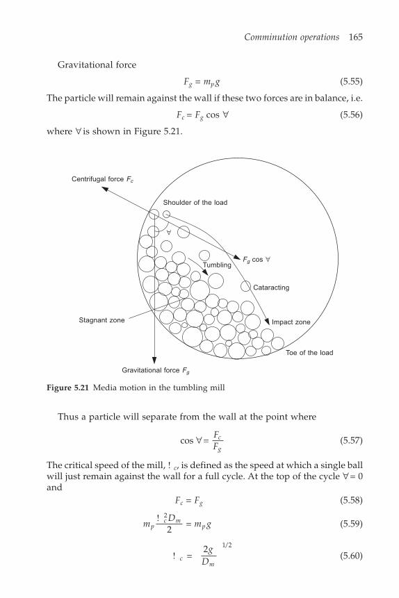
Comminution operations 165
Gravitational force
Fg = mp g (5.55)
The particle will remain against the wall if these two forces are in balance, i.e.
Fc = Fg cos ∀ (5.56)
where ∀ is shown in Figure 5.21.
Centrifugal force Fc
Shoulder of the load
∀
Fg cos ∀Tumbling
Cataracting
Impact zone
Toe of the load
Gravitational force Fg
Stagnant zone
Figure 5.21 Media motion in the tumbling mill
Thus a particle will separate from the wall at the point where
cos = ∀ FF
c
g(5.57)
The critical speed of the mill, ! c, is defined as the speed at which a single ballwill just remain against the wall for a full cycle. At the top of the cycle ∀ = 0and
Fc = Fg (5.58)
mD
m gpc m
p! 2
2 = (5.59)
! cm
gD
= 2 1/2
(5.60)
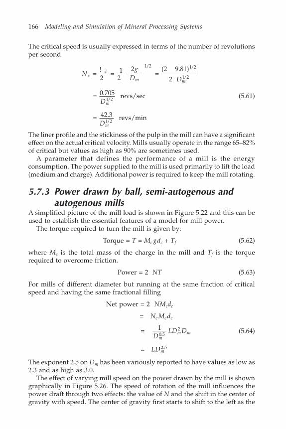
166 Modeling and Simulation of Mineral Processing Systems
The critical speed is usually expressed in terms of the number of revolutionsper second
Ng
D Dc
c
m m =
2 = 1
22
= (2 9.81)
2
1/2 1/2
1/2!
= 0.705 revs/sec1/2Dm
(5.61)
= 42.3 revs/min1/2Dm
The liner profile and the stickiness of the pulp in the mill can have a significanteffect on the actual critical velocity. Mills usually operate in the range 65–82%of critical but values as high as 90% are sometimes used.
A parameter that defines the performance of a mill is the energyconsumption. The power supplied to the mill is used primarily to lift the load(medium and charge). Additional power is required to keep the mill rotating.
5.7.3 Power drawn by ball, semi-autogenous andautogenous mills
A simplified picture of the mill load is shown in Figure 5.22 and this can beused to establish the essential features of a model for mill power.
The torque required to turn the mill is given by:
Torque = T = Mc gdc + Tf (5.62)
where Mc is the total mass of the charge in the mill and Tf is the torquerequired to overcome friction.
Power = 2 NT (5.63)
For mills of different diameter but running at the same fraction of criticalspeed and having the same fractional filling
Net power = 2 NMcdc
= Nc Mc dc
= 10.5
2
DLD D
mm m (5.64)
= 2.5LDm
The exponent 2.5 on Dm has been variously reported to have values as low as2.3 and as high as 3.0.
The effect of varying mill speed on the power drawn by the mill is showngraphically in Figure 5.26. The speed of rotation of the mill influences thepower draft through two effects: the value of N and the shift in the center ofgravity with speed. The center of gravity first starts to shift to the left as the
Comminution operations 167
speed of rotation increases but as critical speed is reached the center of gravitymoves towards the center of the mill as more and more of the material is heldagainst the shell throughout the cycle. Since critical speed is larger at smallerradii the centrifuging layer gets thicker and thicker as the speed increasesuntil the entire charge is centrifuging and the net power draw is zero.
The effect of mill charge is primarily through the shifting of the center ofgravity and the mass of the charge. As the charge increases the center ofgravity moves inward. The power draft is more or less symmetrical about the50% value.
A simple equation for calculating net power draft is:
P D LKc m l = 2.00 kW2.5 (5.65)
Kl is the loading factor which can be obtained from Figure 5.23 for the popularmill types. c is the mill speed measured as a fraction of the critical speed.
More reliable models for the prediction of the power drawn by ball, semi-autogenous and fully autogenous mills have been developed by Morrell (1996)and by Austin (1990). The relationship between gross power and net poweris given by
Figure 5.22 Simplified calculation of the torque required to turn a mill
dc
Fraction J
Center of gravityof the charge
Mcg
168 Modeling and Simulation of Mineral Processing Systems
7
6
5
4
30 10 20 30 40 50 60 70
Dry grate millWet grate millWet overflow mill
Load
ing
fact
or K
L
Load in the mill %
Figure 5.23 Effect of mill filling on power draft for ball mills. The data is taken fromRexnord Process Machinery Reference Manual, Rexnord Process Machinery Division,Milwaukee, 1976
Gross power = No-load power + Net power drawn by the charge (5.66)
The net power is calculated from
Net power = Watts2.5KD Lm e c# (5.67)
In Equation 5.67, Dm is the diameter inside the mill liners and Le is the effectivelength of the mill including the conical ends. #c is the specific gravity of thecharge and and are factors that account for the fractional filling and thespeed of rotation respectively. K is a calibration constant that varies with thetype of discharge. For overflow mills K = 7.98 and for grate mills K = 9.10.This difference is ascribed to the presence of a pool of slurry that is presenton the bottom of overflow-discharge mills but which is not present to thesame extent in grate-discharge mills. This pool is situated more or lesssymmetrically with respect to the axis of the mill and therefore does not drawsignificant power. Austin recommends K = 10.6 for overflow semi-autogenousmills, however a value of K = 9.32 gives a better fit between Austin’s formulaand Morrell’s data and this value is recommended.
The no-load power accounts for all frictional and mechanical losses in thedrive system of the mill and can be calculated from Morrell (1996):
No-load power = 1.68 [ (0.667 + )] kW2.05 0.82D L Lm c d (5.68)
Ld is the mean length of the conical ends and is calculated as half the differencebetween the center-line length of the mill and the length of the cylindrical section.

Comminution operations 169
The geometry of a mill with conical ends is shown in Figure 5.24. The totalvolume inside the mill is given by
V D LL L
LD DD Dm m
c t m
t m =
4 1 +
2( – ) 1 – ( / )1 – /
23
(5.69)
Figure 5.24 Geometry of a mill with cylindrical ends. All dimensions are inside liners.Lc = centerline length, L = belly length, Dm = mill diameter, Dt = trunnion diameter
Lc
L
Dm Dt
The density of the charge must account for all of the material in the millincluding the media which may be steel balls in a ball mill, or large lumps ofore in an autogenous mill or a mixture in a semi-autogenous mill, as well asthe slurry that makes up the operating charge. Let Jt be the fraction of the millvolume that is occupied by the total charge, Jb the fraction of the mill volumethat is occupied by steel balls and E the voidage of the balls and media. U isthe fraction of the voidage that is filled by slurry. v is the volume fraction ofsolids in the slurry. Let VB be the volume of steel balls in the mill, VMed be thevolume of autogenous media and VS the volume of slurry.
VB = Jb(1 – E)Vm
VS = JtUEVm (5.70)
VMed = (Jt – Jb)(1 – E)Vm
The charge density is calculated from
## # #
cB b m S v S v S
t
V V V VJ
= + + (1 – )1000 + Med (5.71)
170 Modeling and Simulation of Mineral Processing Systems
where #b is the density of the balls and #m the density of the media. Theeffective length of the mill is dependent on the load and is calculated from
L L J JLLe t td = 1 + 2.28 (1 – ) (5.72)
according to Morrell and from
Le = L(1 + f3)
fJ J
LL D D J Jt t
d
t t t3
0.1 –4
= 0.092(1 – 1.03 ) (1 – / )
0.6250.5 –
–0.625
0.5 –(5.73)
according to Austin.The functions and account for the effects of mill filling and rotation
speed respectively. However each of these factors is a function of both millfilling and rotation speed. Morrell recommends the following formulas:
!!
= ( – )
2
J Jt t (5.74)
! = 2(2.986 – 2.213 – 0.4927)2c c
and
= (1 – [1 – ] exp(–19.42( – ))) = 0.954 – 0.135
max max
max
c c
tJ(5.75)
Austin recommends the following formulas for the factors and :
= (1 – 1.03 )
= 1 –0.1
29–10
J Jt t
cc
(5.76)
The formulas proposed by Austin and Morrell give substantially the sameestimates of the net power that is drawn by the mill. Some typical cases areshown in Figure 5.25.
5.7.4 Power drawn by rod millsThe power drawn by a rod mill is given by:
P = 1.752D0.33(6.3 – 5.4Vp) c kW hr/tonne of rods charged (5.77)
where Vp = fraction of the mill volume that is loaded with rods. Rod millsoperate typically at c between 0.64 and 0.75 with larger diameter mills runningat the lower end and smaller mills at the upper end. Typical rod loads are35% to 45% of mill volume and rod bulk densities range from about 5400 kg/m3 to 6400 kg/m3 (Rowland and Kjos, 1980).
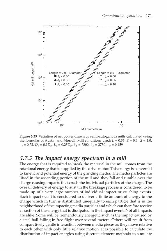
Comminution operations 171
5.7.5 The impact energy spectrum in a millThe energy that is required to break the material in the mill comes from therotational energy that is supplied by the drive motor. This energy is convertedto kinetic and potential energy of the grinding media. The media particles arelifted in the ascending portion of the mill and they fall and tumble over thecharge causing impacts that crush the individual particles of the charge. Theoverall delivery of energy to sustain the breakage process is considered to bemade up of a very large number of individual impact or crushing events.Each impact event is considered to deliver a finite amount of energy to thecharge which in turn is distributed unequally to each particle that is in theneighborhood of the impacting media particles and which can therefore receivea fraction of the energy that is dissipated in the impact event. Not all impactsare alike. Some will be tremendously energetic such as the impact caused bya steel ball falling in free flight over several meters. Others will result fromcomparatively gentle interaction between media pieces as they move relativeto each other with only little relative motion. It is possible to calculate thedistribution of impact energies using discrete element methods to simulate
104
103
102
101
100
100 101
Length = 2.0 DiameterJb = 0.00Jb = 0.05
Jb = 0.10
Length = 0.5 DiameterJb = 0.00Jb = 0.05
Jb = 0.10
Mill diameter m
Net
mill
pow
er k
W
Figure 5.25 Variation of net power drawn by semi-autogenous mills calculated usingthe formulas of Austin and Morrell. Mill conditions used: Jt = 0.35, E = 0.4, U = 1.0,
c = 0.72, Do = 0.1Dm, Ld = 0.25Dm, #B = 7800, #S = 2750, v = 0.459
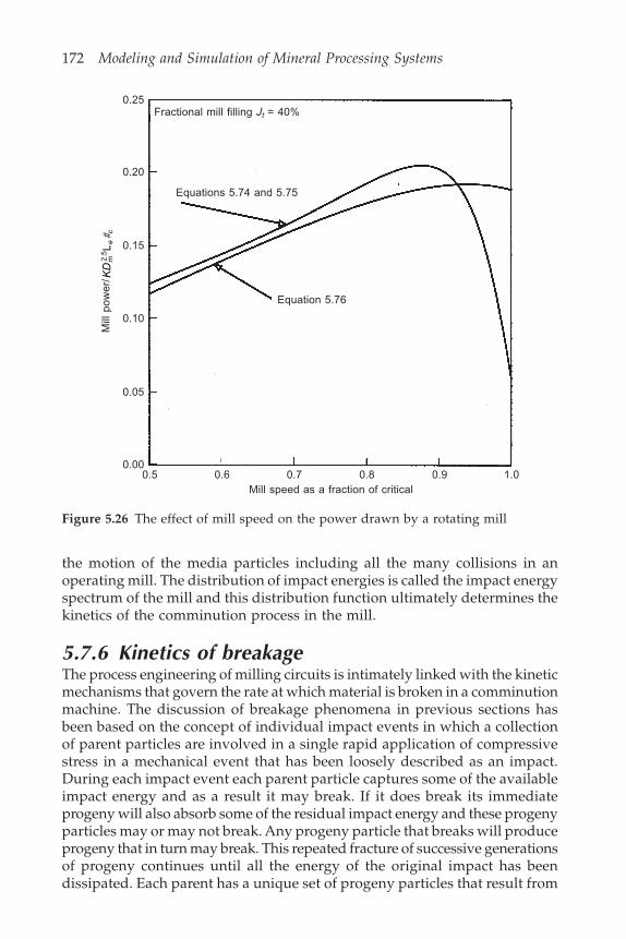
172 Modeling and Simulation of Mineral Processing Systems
the motion of the media particles including all the many collisions in anoperating mill. The distribution of impact energies is called the impact energyspectrum of the mill and this distribution function ultimately determines thekinetics of the comminution process in the mill.
5.7.6 Kinetics of breakageThe process engineering of milling circuits is intimately linked with the kineticmechanisms that govern the rate at which material is broken in a comminutionmachine. The discussion of breakage phenomena in previous sections hasbeen based on the concept of individual impact events in which a collectionof parent particles are involved in a single rapid application of compressivestress in a mechanical event that has been loosely described as an impact.During each impact event each parent particle captures some of the availableimpact energy and as a result it may break. If it does break its immediateprogeny will also absorb some of the residual impact energy and these progenyparticles may or may not break. Any progeny particle that breaks will produceprogeny that in turn may break. This repeated fracture of successive generationsof progeny continues until all the energy of the original impact has beendissipated. Each parent has a unique set of progeny particles that result from
0.25
0.20
0.15
0.10
0.05
0.000.5 0.6 0.7 0.8 0.9 1.0
Mill speed as a fraction of critical
Mill
pow
er/ K
Dm
ec
2.5L
#
Equation 5.76
Equations 5.74 and 5.75
Fractional mill filling Jt = 40%
Figure 5.26 The effect of mill speed on the power drawn by a rotating mill

Comminution operations 173
the impact and each progeny comes from one and only one original parent.The distribution of sizes of the set of progeny particles is defined by thebreakage function of the parent. These discrete impact events happen withhigh frequency in a grinding mill and it is convenient to consider the breakageas a continuous process. This provides an effective modeling method that isbased on the population balance approach.
In any region of a comminution machine, the rate at which material of aparticular size is being broken is a strong function of the amount of that sizeof material present. This is the basis of the model. The rate of breakage varieswith size. It is convenient to use discrete size classes that provide an adequateapproximation for practical computation.
The fundamental postulate that supports the kinetic model is that the rateof breakage of material out of size class i is proportional to the amount ofmaterial of size i in the mill. Thus
Rate of breakage = ki Mmi
ki is called the specific rate of breakage. It is also called the selection function.Note that ki is a function of the representative size in the class. It may also bea function of the composition of the parent particle.
Material breaking out of class i distributes itself over all other classesaccording to the breakage function which is specific to the comminutionoperation and the material being broken.
It is common practice to normalize the breakage function to the lowermesh size of the interval so that breakage means breakage out of a size class.If the breakage function is described by the standard form:
B x y Kxy
Kxy
n n
( ; ) = + (1 – )1 2
(5.78)
then
bij = B(Di–1; Dj) – B(Di; Dj) (5.79)
bjj = 0
The relationship between the cumulative breakage function and bij is shownin Figure 5.27. The breakage function has the value 1.0 at the lower boundaryof the parent size interval. This reflects the convention that breakage is assumedto occur only when material leaves the parent size interval. This conventionhas been adopted because it is only possible to detect breakage in a laboratoryexperiment if the material leaves the sieve interval. The convention is not anessential feature of the population balance method but it is convenient becausemost of the breakage data that appears in the literature has it as the base. Atall events it is not difficult to convert the breakage function data to the alternativeconvention if required. The differences between Equation 5.79 and theequivalent expressions for crushing machines (5.52 and 5.53) should be noted.
If normalization is satisfactory and if a strictly geometric progression is

174 Modeling and Simulation of Mineral Processing Systems
used for the mess size then bij is a function only of the difference i – j. Forexample if a root 2 series is used for the size classes.
DD
DD
i
j
ii j
i
j i = ( 2 )
= ( 2 )–
– (5.80)
b KDD
KDD
KDD
KDDij
i
j
ni
j
ni
j
ni
j
n
= + (1 – ) – + (1 – )–1 –11 2 1 2
(5.81)
b K Kijn j i n j i n j i n j i
= [( 2 ) – ( 2 ) ] + (1 – )[( 2 ) – 2 ]1 1 2 2( – +1) ( – ) ( – +1) ( – )
= ( 2 ) ( 2 – 1) + (1 – )( 2 ) ( 2 – 1)1 2( – ) ( – )K Kn j i n j i (5.82)
= 0.414 ( 2 ) + 0.414(1 – )( 2 )1 2( – ) ( – )K Kn j i n j i
5.8 The continuous millIndustrial grinding mills always process material continuously so that modelsmust simulate continuous operation. Suitable models are developed in thissection.
1.0
0.0
Bre
akag
e fu
nctio
n B
(dp;
dj)
Di Di–1 Dj Dj–1
Particle size
bij
Figure 5.27 The breakage function used for the description of milling operations inrotating mills. Compare with the equivalent diagram for crushing machines (Figure5.19)
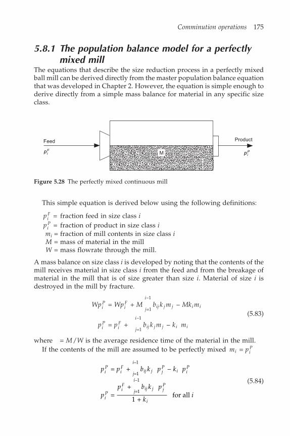
Comminution operations 175
5.8.1 The population balance model for a perfectlymixed mill
The equations that describe the size reduction process in a perfectly mixedball mill can be derived directly from the master population balance equationthat was developed in Chapter 2. However, the equation is simple enough toderive directly from a simple mass balance for material in any specific sizeclass.
Figure 5.28 The perfectly mixed continuous mill
M
Feed
piF
Product
piP
This simple equation is derived below using the following definitions:
piF = fraction feed in size class i
piP = fraction of product in size class i
mi = fraction of mill contents in size class iM = mass of material in the millW = mass flowrate through the mill.
A mass balance on size class i is developed by noting that the contents of themill receives material in size class i from the feed and from the breakage ofmaterial in the mill that is of size greater than size i. Material of size i isdestroyed in the mill by fracture.
Wp Wp M b k m Mk m
p p b k m k m
iP
iF
j
i
ij j j i i
iP
iF
j
i
ij j j i i
= + –
= + –
=1
–1
=1
–1(5.83)
where = M/W is the average residence time of the material in the mill.If the contents of the mill are assumed to be perfectly mixed m pi i
P =
p p b k p k p
pp b k p
ki
iP
iF
j
i
ij j jP
i iP
iP
iF
j
i
ij j jP
i
= + –
= +
1 + for all
=1
–1
=1
–1 (5.84)

176 Modeling and Simulation of Mineral Processing Systems
Well-mixed zone
These can be solved by a straightforward recursion relationship starting withsize class 1.
pp
kP
F
11
1 =
1 +
pp b k p
kP
F P
22 21 1 1
2 =
+ 1 +
(5.85)
pp b k p b k p
kP
F P P
33 31 1 1 32 2 2
3 =
+ + 1 +
etc.
5.8.2 The mill with post classificationIn practice the material in the mill does not have unrestricted ability to leavein the outlet stream. Larger particles are prevented from leaving by the dischargegrate if one is present and even in overflow discharge mills, the larger particlesdo not readily move upward through the medium bed to the discharge. Onthe other hand very small particles move readily with the water and aredischarged easily. Thus the discharge end of the mill behaves as a classifierwhich permits the selective discharge of smaller particles and recycles thelarger particles back into the body of the mill. This is illustrated schematicallyin Figure 5.29. The operation of such a mill can be modeled as a perfectlymixed mill with post classification as shown in Figure 5.30.
Return of oversize
Postclassification Product
Feed
Figure 5.29 The classification mechanism at the mill discharge end recycles largerparticles into the body of the mill
Applying Equation 5.84 to the perfectly mixed milling section:
mf b k m
ki
i j
i
ij j j
i =
+
1 + =1
–1
(5.86)
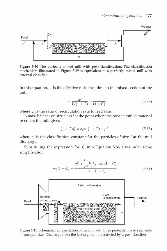
Comminution operations 177
In this equation, is the effective residence time in the mixed section of themill:
= (1 + )
= (1 + )
MW C C
(5.87)
where C is the ratio of recirculation rate to feed rate.A mass balance on size class i at the point where the post classified material
re-enters the mill gives
(1 + ) = (1 + ) + C f c m C pi i i iF (5.88)
where ci is the classification constant for the particles of size i at the milldischarge.
Substituting the expression for fi into Equation 5.84 gives, after somesimplification,
m Cp b k m C
k ci
iF
j
i
ij j j
i i(1 + ) =
+ (1 + )
1 + –=1
–1
(5.89)
M
Feed
piF
Product
piP
pi
C
Figure 5.30 The perfectly mixed mill with post classification. The classificationmechanism illustrated in Figure 5.29 is equivalent to a perfectly mixed mill withexternal classifier
Figure 5.31 Schematic representation of the mill with three perfectly mixed segmentsof unequal size. Discharge from the last segment is restricted by a post classifier
Main mixing zone
Feed
Smallermixing zones
Return of oversize
Postclassification Product
fi
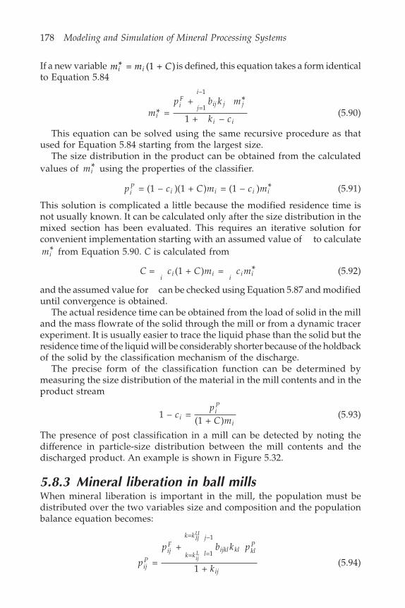
178 Modeling and Simulation of Mineral Processing Systems
If a new variable m m Ci i* = (1 + ) is defined, this equation takes a form identicalto Equation 5.84
mp b k m
k ci
iF
j
i
ij j j
i i* =
+ *
1 + –=1
–1
(5.90)
This equation can be solved using the same recursive procedure as thatused for Equation 5.84 starting from the largest size.
The size distribution in the product can be obtained from the calculatedvalues of mi* using the properties of the classifier.
p c C m c miP
i i i i = (1 – )(1 + ) = (1 – ) * (5.91)
This solution is complicated a little because the modified residence time isnot usually known. It can be calculated only after the size distribution in themixed section has been evaluated. This requires an iterative solution forconvenient implementation starting with an assumed value of to calculatemi* from Equation 5.90. C is calculated from
C c C m c mi i i i i i = (1 + ) = * (5.92)
and the assumed value for can be checked using Equation 5.87 and modifieduntil convergence is obtained.
The actual residence time can be obtained from the load of solid in the milland the mass flowrate of the solid through the mill or from a dynamic tracerexperiment. It is usually easier to trace the liquid phase than the solid but theresidence time of the liquid will be considerably shorter because of the holdbackof the solid by the classification mechanism of the discharge.
The precise form of the classification function can be determined bymeasuring the size distribution of the material in the mill contents and in theproduct stream
1 – = (1 + )
cpC miiP
i(5.93)
The presence of post classification in a mill can be detected by noting thedifference in particle-size distribution between the mill contents and thedischarged product. An example is shown in Figure 5.32.
5.8.3 Mineral liberation in ball millsWhen mineral liberation is important in the mill, the population must bedistributed over the two variables size and composition and the populationbalance equation becomes:
p
p b k p
kijP
ijF
k k
k k
l
j
ijkl kl klP
ij
ijL
IJU
=
+
1 +
=
=
=1
–1
(5.94)
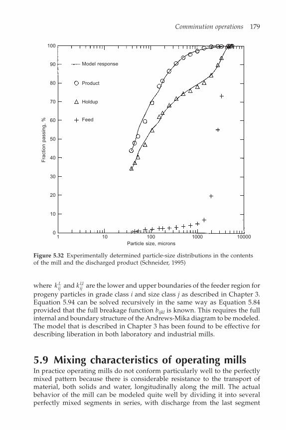
Comminution operations 179
where k kijL
ijU and are the lower and upper boundaries of the feeder region for
progeny particles in grade class i and size class j as described in Chapter 3.Equation 5.94 can be solved recursively in the same way as Equation 5.84provided that the full breakage function bijkl is known. This requires the fullinternal and boundary structure of the Andrews-Mika diagram to be modeled.The model that is described in Chapter 3 has been found to be effective fordescribing liberation in both laboratory and industrial mills.
5.9 Mixing characteristics of operating millsIn practice operating mills do not conform particularly well to the perfectlymixed pattern because there is considerable resistance to the transport ofmaterial, both solids and water, longitudinally along the mill. The actualbehavior of the mill can be modeled quite well by dividing it into severalperfectly mixed segments in series, with discharge from the last segment
100
90
80
70
60
50
40
30
20
10
01 10 100 1000 10000
Particle size, microns
Fra
ctio
n pa
ssin
g, %
Model response
Product
Holdup
Feed
Figure 5.32 Experimentally determined particle-size distributions in the contentsof the mill and the discharged product (Schneider, 1995)
180 Modeling and Simulation of Mineral Processing Systems
being restricted by a post classifier. The size distribution in the material thatleaves each segment can be calculated by repeated application of Equation5.84 successively to each mixed segment in turn. The product from the firstsegment becomes the feed to the next and so on down the mill. The numberof mixed sections and their relative sizes can be determined from the residence-time distribution function in the mill. Residence distribution functions havebeen measured in a number of operating ball, pebble and autogenous millsand it is not unusual to find that three unequal perfectly mixed segments areadequate to describe the measured residence-time distribution functions.Usually the last segment is significantly larger than the other two. This isconsistent with the behavior of a post classifier that holds up the largerparticles at the discharge end of the mill, which are then thrown quite farback into the body of the mill.
It has been suggested in the literature that a further refinement to themixed-region model can be achieved by the use of a classification actionbetween each pair of segments, but since it is impossible to make independentlyverifiable measurements of such inter-stage classifications, this refinementcannot be used effectively.
The structure of a mill with three perfectly-mixed segments with postclassification on the last is illustrated in Figure 5.31.
The residence-time distribution function for a mill can be measuredexperimentally by means of a dynamic tracer test. It is considerably easier totrace the liquid phase than the solid phase and this is usually done in practicebut the two phases have significantly different residence-time distributions.The water is not restricted during its passage through the mill as much as thesolid phase is. Consequently the hold-up of solid in the mill is greater thanthat of the liquid and the solid has a higher mean residence time. Althoughthe two phases have significantly different mean residence times, the behaviorof each phase is consistent with the three-stage model that is described above.This is demonstrated in the two measured residence-time distributions thatare shown in Figures 5.33 and 5.34. The data shown in Figures 5.33 and 5.34were collected from the same mill. The solid phase was traced by adding asample of silica rapidly to the feed stream, which was normally limestone.The mill product was sampled frequently and the concentration of SiO2 ineach sample by X-ray fluorescence analysis. The liquid was traced by rapidlyadding a small sample of water-soluble colored tracer to the mill feed andanalyzing the liquid phase in the product samples by UV absorbance.
5.10 Models for rod millsThe physical arrangement of rods in the rod mill inhibits the effective internalmixing that is characteristic of ball mills. The axial mixing model for themixing pattern is more appropriate than that based on the perfectly-mixedregion. When axial mixing is not too severe in the mill, an assumption of plugflow is appropriate. In that case the population balance model for the batch

Comminution operations 181
mill can be used to simulate the behavior of the rod mill with the time replacedby the average residence time in the mill which is equal to the holdup dividedby the throughput.
5.11 The population balance model forautogenous mills
Four distinct mechanisms of size reduction have been identified in fullyautogenous mills: attrition, chipping, impact fracture and self-breakage.Attrition is the steady wearing away of comparatively smooth surfaces oflumps due to friction between the surfaces in relative motion. Chipping occurswhen asperities are chipped off the surface of a particle by contacts that arenot sufficiently vigorous to shatter the particle. Attrition and chipping areessentially surface phenomena and are commonly lumped together andidentified as wear processes. Impact fracture occurs when smaller particlesare nipped between two large particles during an impact induced by collisionor rolling motion. Self-breakage occurs when a single particle shatters onimpact after falling freely in the mill. Rates of breakage and the progeny
2.8
2.4
2.0
1.6
1.2
0.8
0.4
0.00 15 30 45 60 75 90 105 120 135 150
Time, minutes
Abs
orba
nce
RTD model response
Experimental
tau 1 =15.177tau 2 = 0.629tau 3 = 0.384
Figure 5.33 Residence-time distribution function for the water in a continuous ballmill. The line shows the small-small-large segment model response to this experimentaldata. Note the smaller residence times than for the solid phase in the same mill shownin Figure 5.34 (Schneider, 1995)
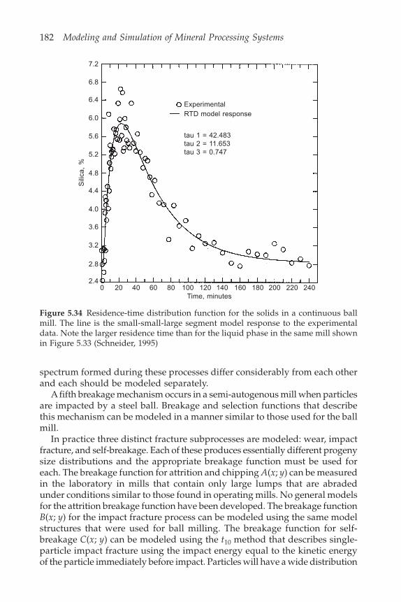
182 Modeling and Simulation of Mineral Processing Systems
spectrum formed during these processes differ considerably from each otherand each should be modeled separately.
A fifth breakage mechanism occurs in a semi-autogenous mill when particlesare impacted by a steel ball. Breakage and selection functions that describethis mechanism can be modeled in a manner similar to those used for the ballmill.
In practice three distinct fracture subprocesses are modeled: wear, impactfracture, and self-breakage. Each of these produces essentially different progenysize distributions and the appropriate breakage function must be used foreach. The breakage function for attrition and chipping A(x; y) can be measuredin the laboratory in mills that contain only large lumps that are abradedunder conditions similar to those found in operating mills. No general modelsfor the attrition breakage function have been developed. The breakage functionB(x; y) for the impact fracture process can be modeled using the same modelstructures that were used for ball milling. The breakage function for self-breakage C(x; y) can be modeled using the t10 method that describes single-particle impact fracture using the impact energy equal to the kinetic energyof the particle immediately before impact. Particles will have a wide distribution
Figure 5.34 Residence-time distribution function for the solids in a continuous ballmill. The line is the small-small-large segment model response to the experimentaldata. Note the larger residence time than for the liquid phase in the same mill shownin Figure 5.33 (Schneider, 1995)
Experimental
tau 1 = 42.483tau 2 = 11.653tau 3 = 0.747
RTD model response
7.2
6.8
6.4
6.0
5.6
5.2
4.8
4.4
4.0
3.6
3.2
2.8
2.40 20 40 60 80 100 120 140 160 180 200 220 240
Time, minutes
Sili
ca,
%

Comminution operations 183
of free-fall impact energies in a real mill and the breakage function for self-breakage is obtained by integration over the impact energy spectrum
C x y C x y h P y h p h dh( ; ) = ( ; , ) ( , ) ( ) 0
(5.95)
where C(x; y, h) is the single particle breakage function for self-breakage of aparticle of size y in free fall from height h, P(y, h) is the probability that aparticle of size y will shatter when falling a vertical height h and p(h) is thedistribution density for effective drop heights in the mill.
The attrition and wear processes that occur in autogenous, semi-autogenous,and pebble mills produce a significant fraction of the final production of fineparticles in the mill. These processes are not satisfactorily described by thekinetic breakage models that are useful for ball and rod mills. It is necessaryto invoke the full generalized population balance model that was developedin Section 2.14 in order to describe the autogenous milling operationsadequately.
Various finite difference representations of Equation 2.116 are availablebut those based on the predefined size classes as described in Chapter 2 aregenerally used. It is usual and useful to interpret the rate of breakage process� in such a way that
D
D
i ii
i
p x x F p x dx R p x F p x–1
( ( ), , [ ( )]) = ( , , [ ( )])� (5.96)
is the rate of breakage out of the interval i. This convention, which was usedto develop the simple finite difference models for ball and rod mills, is usefulparticularly because it is comparatively easy to measure the rate of breakageout of a screen interval in the laboratory and to correlate the measured rateswith the representative size for a size class.
Equation 2.116 is integrated over a typical size class i to give
– ( ) + 3 ( )( )
+ ( , , [ ( )])–1
1iD
D
i ip x xp x
xdx R p x F p x
i
i
– ( , , [ ( )] ( , )=1
–1
1j
i
j j i jR p x F p x B x D
– 3 ( ) ( )
( ; )–1
( )D
D
R xi
i
xp x
xa x x dx dx (5.97)
= Pi in – Pi out
where
i p(x) = (Di–1)p(Di–1) – (Di)p(Di) (5.98)
and
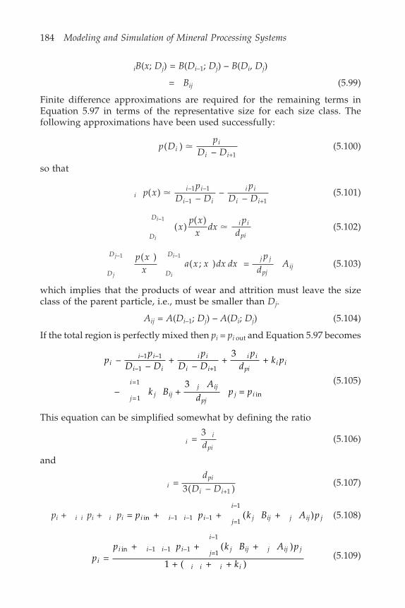
184 Modeling and Simulation of Mineral Processing Systems
iB(x; Dj) = B(Di–1; Dj) – B(Di, Dj)
= Bij (5.99)
Finite difference approximations are required for the remaining terms inEquation 5.97 in terms of the representative size for each size class. Thefollowing approximations have been used successfully:
p D
pD Di
i
i i( )
– +1� (5.100)
so that
i
i i
i i
i i
i ip x
pD D
pD D
( ) –
––
–1 –1
–1 +1� (5.101)
D
Di i
pii
i
xp x
xdx
pd
–1
( )( )
� (5.102)
D
D
D
Dj j
pjij
j
j
i
ip xx
a x x dx dxp
dA
–1 –1( ) ( ; ) = (5.103)
which implies that the products of wear and attrition must leave the sizeclass of the parent particle, i.e., must be smaller than Dj.
Aij = A(Di–1; Dj) – A(Di; Dj) (5.104)
If the total region is perfectly mixed then pi = pi out and Equation 5.97 becomes
pp
D Dp
D Dp
dk p
k BA
dp p
ii i
i i
i i
i i
i i
pii i
j
i
j ijj ij
pjj i
––
+ –
+ 3
+
– + 3
=
–1 –1
–1 +1
=1
=1
in
(5.105)
This equation can be simplified somewhat by defining the ratio
ii
pid =
3(5.106)
and
ipi
i i
dD D
= 3( – )+1
(5.107)
pi + i i pi + i pi = + + ( + )in –1 –1 –1 =1
–1
p p k B A pi i i i j
i
j ij j ij j (5.108)
pp p k B A p
ki
i i i i j
i
j ij j ij j
i i i i =
+ + ( + )
1 + ( + + )
in –1 –1 –1 =1
–1
(5.109)
Comminution operations 185
This equation can be simplified further by making the following definitions:
i = i i (5.110)
i = (ki + i) (5.111)
Both N and N are zero because there is no breakage out of the smallest sizeclass.
(kj Bij + j Aij) = ij (5.112)
Using the definitions of Aij and Bij
i j
N
ij j j jk= +1
= ( + ) = (5.113)
Equation 5.109 can be written
pP p p
i
i i i j
i
ij j
i i =
+ +
+ + 1
in –1 –1 =1
–1
(5.114)
This is the fundamental discrete population balance equation for autogenousmills and it should be compared with the equivalent Equation 5.84 for theball mill. The appearance of the term pi–1 on the right hand side of Equation5.114 should be particularly noted. This term arises from the wear processthat reduces the size of large lumps in the mill charge which is an essentialfeature of autogenous milling. Equation 5.114 can be solved recursively in astraightforward manner starting at p0. However it is necessary to choose avalue of 0p0 to ensure that
i
N
ip=1
= 1 (5.115)
is satisfied.Using Equation 5.114
i
N
i i i i
N
i i
N
i i i
N
j
i
ij jp p p p=1 =1 in =1 –1 –1 =1 =1
–1
(1 + + ) = + +
= 1 + + + 0 0 =2 –1 –1 =1
–1
= +1p p p
i
N
i i j
N
j i j
N
ij (5.116)
= 1 + + + 0 0 =1
–1
=1
–1
p p pj
N
j j j
N
j j
= 1 + + ( + )0 0 =1
–1
p pj
N
j j j
which leads to
186 Modeling and Simulation of Mineral Processing Systems
i
N
i N N Np p p=1 0 0 + ( + ) = 1 + (5.117)
Thus the condition
0p0 = 0 (5.118)
guarantees the consistency of the solution.
5.11.1 The effect of the discharge grateIn practice it is always necessary to maintain some classification action at themill discharge to ensure that large pebbles do not escape from the mill.Autogenous and semi-autogenous mills are always equipped with a steel orrubber grate to hold back the grinding media. The classification action of thegrate can be described in terms of a classification function ci as was done inSection 5.8.2. Application of Equation 5.114 to the mill contents gives
mf m m
i
i i i j
i
ij j
i i =
+ +
1 + +
–1 –1 =1
–1
(5.119)
where
fp
Cc mi
iF
i i = 1 +
+ (5.120)
and C is the fraction of the total stream that is returned to the mill by theclassification action at the discharge end. The residence time to be used tocalculate i, i, and ij in Equation 5.119 is
= (1 + )
= 1 +
MC W C
(5.121)
m
pC
m m
ci
iF
i i j
i
ij j
i i i = 1 +
+ +
1 + + –
–1 –1 =1
–1
(5.122)
Define a new variable
m C mi i* = (1 + ) (5.123)
and this equation becomes
mp m m
ci
iF
i i j
i
ij j
i i i* =
+ * + *
1 + + –
–1 –1 =1
–1
(5.124)
which can be solved recursively starting from i = 1 and 0 0* = 0.m The valueof must be established by iterative calculation using Equation 5.121 after Cis recovered from
Comminution operations 187
C c C m c mi
N
i i i
N
i i = (1 + ) = *=1 =1
(5.125)
The iterative calculation starts from an assumed value of and is continueduntil the value of stabilizes. The size distribution from the mill is recoveredfrom
p c mi i i = (1 – ) * (5.126)
The kinetic parameters ki and i and the breakage functions A(Di; Dj) andB(Di; Dj) must be estimated from experimental data.
5.12 Models for the specific rate of breakagein ball mills
The utility the kinetic model for breakage depends on the availability ofrobust models for the specific rate of breakage to describe specific millingconditions. Both functions are strong functions of the milling environment.Factors which affect the rate of breakage are the mill diameter, mill speed,media load and size and particle hold-up.
The most important functional dependence is between the specific rate ofbreakage and the particle size and methods for the description of thisfunctional dependence are described below. The specific rate of breakageincreases steadily with particle size which reflects the decreasing strength ofthe particles as size increases. This is attributed to the greater density ofmicroflaws in the interior of larger particles and to the greater likelihoodthat a particular large particle will contain a flaw that will initiate fractureunder the prevailing stress conditions in a mill. The decrease in particlestrength does not lead to an indefinite increase in the specific rate of breakage.As the particle size becomes significant by comparison to the size of thesmallest media particles, the prevailing stress levels in the mill are insufficientto cause fracture and the specific rate of breakage passes through a maximumand decreases with further increase in particle size. Some typical data areshown in Figure 5.35.
5.12.1 The Austin model for the specific rate ofbreakage
Austin represents the variation of the specific rate of breakage with particlesize by the function
k dS d
dp
p
p( ) =
1 + ( / )1
(5.127)
and it is usual to specify the particle size in mm and the specific rate ofbreakage in min–1.
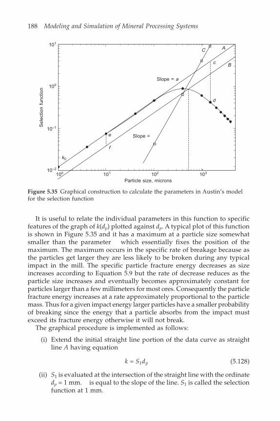
188 Modeling and Simulation of Mineral Processing Systems
It is useful to relate the individual parameters in this function to specificfeatures of the graph of k(dp) plotted against dp. A typical plot of this functionis shown in Figure 5.35 and it has a maximum at a particle size somewhatsmaller than the parameter which essentially fixes the position of themaximum. The maximum occurs in the specific rate of breakage because asthe particles get larger they are less likely to be broken during any typicalimpact in the mill. The specific particle fracture energy decreases as sizeincreases according to Equation 5.9 but the rate of decrease reduces as theparticle size increases and eventually becomes approximately constant forparticles larger than a few millimeters for most ores. Consequently the particlefracture energy increases at a rate approximately proportional to the particlemass. Thus for a given impact energy larger particles have a smaller probabilityof breaking since the energy that a particle absorbs from the impact mustexceed its fracture energy otherwise it will not break.
The graphical procedure is implemented as follows:
(i) Extend the initial straight line portion of the data curve as straightline A having equation
k S dp = 1 (5.128)
(ii) S1 is evaluated at the intersection of the straight line with the ordinatedp = 1 mm. is equal to the slope of the line. S1 is called the selectionfunction at 1 mm.
101
100
10–1
10–2
100 101 102 103
Sel
ectio
n fu
nctio
n
k0
e
f
Slope = a
Slope =
c
d
A
B
Particle size, microns
C
Figure 5.35 Graphical construction to calculate the parameters in Austin’s modelfor the selection function
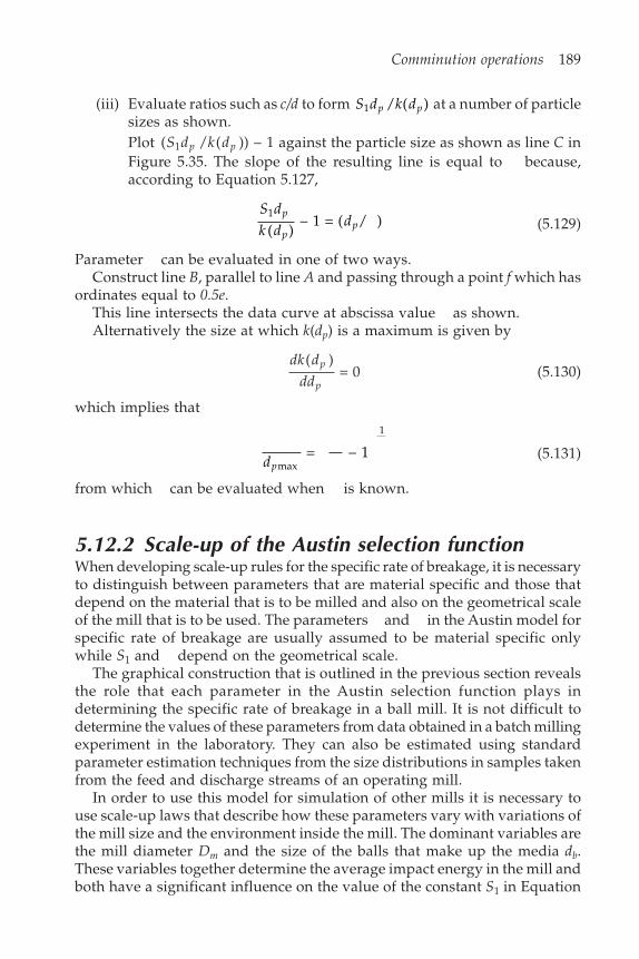
Comminution operations 189
(iii) Evaluate ratios such as c/d to form S d k dp p1 / ( ) at a number of particlesizes as shown.Plot ( / ( )) – 11S d k dp p against the particle size as shown as line C inFigure 5.35. The slope of the resulting line is equal to because,according to Equation 5.127,
S dk d
dp
pp
1
( )– 1 = ( / ) (5.129)
Parameter can be evaluated in one of two ways.Construct line B, parallel to line A and passing through a point f which has
ordinates equal to 0.5e.This line intersects the data curve at abscissa value as shown.Alternatively the size at which k(dp) is a maximum is given by
dk ddd
p
p
( ) = 0 (5.130)
which implies that
dpmax
1
= – 1 (5.131)
from which can be evaluated when is known.
5.12.2 Scale-up of the Austin selection functionWhen developing scale-up rules for the specific rate of breakage, it is necessaryto distinguish between parameters that are material specific and those thatdepend on the material that is to be milled and also on the geometrical scaleof the mill that is to be used. The parameters and in the Austin model forspecific rate of breakage are usually assumed to be material specific onlywhile S1 and depend on the geometrical scale.
The graphical construction that is outlined in the previous section revealsthe role that each parameter in the Austin selection function plays indetermining the specific rate of breakage in a ball mill. It is not difficult todetermine the values of these parameters from data obtained in a batch millingexperiment in the laboratory. They can also be estimated using standardparameter estimation techniques from the size distributions in samples takenfrom the feed and discharge streams of an operating mill.
In order to use this model for simulation of other mills it is necessary touse scale-up laws that describe how these parameters vary with variations ofthe mill size and the environment inside the mill. The dominant variables arethe mill diameter Dm and the size of the balls that make up the media db.These variables together determine the average impact energy in the mill andboth have a significant influence on the value of the constant S1 in Equation
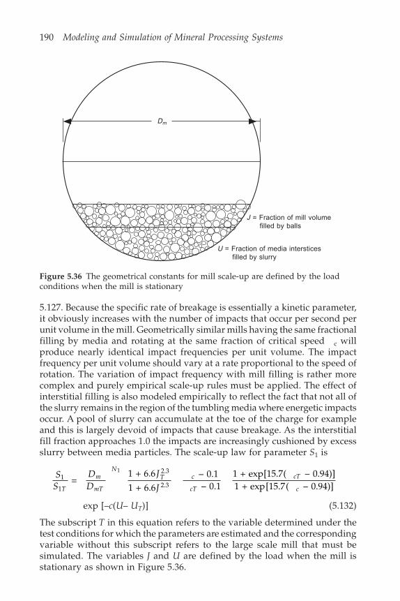
190 Modeling and Simulation of Mineral Processing Systems
5.127. Because the specific rate of breakage is essentially a kinetic parameter,it obviously increases with the number of impacts that occur per second perunit volume in the mill. Geometrically similar mills having the same fractionalfilling by media and rotating at the same fraction of critical speed c willproduce nearly identical impact frequencies per unit volume. The impactfrequency per unit volume should vary at a rate proportional to the speed ofrotation. The variation of impact frequency with mill filling is rather morecomplex and purely empirical scale-up rules must be applied. The effect ofinterstitial filling is also modeled empirically to reflect the fact that not all ofthe slurry remains in the region of the tumbling media where energetic impactsoccur. A pool of slurry can accumulate at the toe of the charge for exampleand this is largely devoid of impacts that cause breakage. As the interstitialfill fraction approaches 1.0 the impacts are increasingly cushioned by excessslurry between media particles. The scale-up law for parameter S1 is
SS
DD
J
JT
m
mT
NT c
cT
cT
c
1
1
2.3
2.3 = 1 + 6.6
1 + 6.6– 0.1– 0.1
1 + exp[15.7( – 0.94)]1 + exp[15.7( – 0.94)]
1
exp [–c(U– UT)] (5.132)
The subscript T in this equation refers to the variable determined under thetest conditions for which the parameters are estimated and the correspondingvariable without this subscript refers to the large scale mill that must besimulated. The variables J and U are defined by the load when the mill isstationary as shown in Figure 5.36.
Dm
J = Fraction of mill volumefilled by balls
U = Fraction of media intersticesfilled by slurry
Figure 5.36 The geometrical constants for mill scale-up are defined by the loadconditions when the mill is stationary
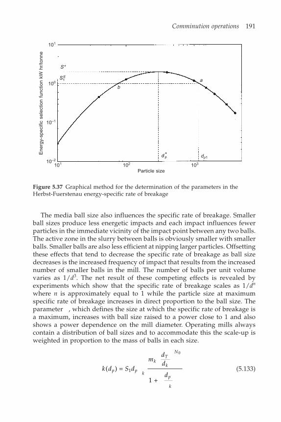
Comminution operations 191
Figure 5.37 Graphical method for the determination of the parameters in theHerbst-Fuerstenau energy-specific rate of breakage
101
100
10–1
10–2
101 102 103
dp1
ba
S*
S E1
d p*E
nerg
y-sp
ecifi
c se
lect
ion
func
tion
kW h
r/to
nne
Particle size
The media ball size also influences the specific rate of breakage. Smallerball sizes produce less energetic impacts and each impact influences fewerparticles in the immediate vicinity of the impact point between any two balls.The active zone in the slurry between balls is obviously smaller with smallerballs. Smaller balls are also less efficient at nipping larger particles. Offsettingthese effects that tend to decrease the specific rate of breakage as ball sizedecreases is the increased frequency of impact that results from the increasednumber of smaller balls in the mill. The number of balls per unit volumevaries as 1/d3. The net result of these competing effects is revealed byexperiments which show that the specific rate of breakage scales as 1/dn
where n is approximately equal to 1 while the particle size at maximumspecific rate of breakage increases in direct proportion to the ball size. Theparameter , which defines the size at which the specific rate of breakage isa maximum, increases with ball size raised to a power close to 1 and alsoshows a power dependence on the mill diameter. Operating mills alwayscontain a distribution of ball sizes and to accommodate this the scale-up isweighted in proportion to the mass of balls in each size.
k d S dm
dd
dp p
k
kT
k
N
p
k
( ) =
1 +
1
0
(5.133)

192 Modeling and Simulation of Mineral Processing Systems
where dk is the representative diameter of the kth ball size class and mk is themass fraction of the ball size class in the mill charge. k is given by
k
kT
m
mT
Nk
T
NDD
dd
= 2 3
(5.134)
Recommended values for the constants are N0 = 1.0, N1 = 0.5, N2 = 0.2, N3 =1.0 and c = 1.3. Large size ball mills have been observed to operate inefficientlyso that it is often recommended that S1 should be scaled by the factor (3.81/Dm)0.2 when the diameter of this type of mill exceeds 3.81 meters.
5.12.3 The Herbst-Fuerstenau model for the specificrate of breakage
The variation of the specific rate of breakage and of the breakage functionwith milling conditions can be substantially accounted for by describing thevariation of these functions with the specific power input into the mill andexamining how the specific power input varies with mill size and with designand operating conditions. This indirect method is particularly useful for scalingup the functions from batch scale and pilot scale test work. This is called theenergy-specific scale-up procedure and was developed initially by Herbstand Fuerstenau (1980).
The specific rate of breakage out of size class i is proportional to the netspecific power input to the mill charge.
k S PMi i
E = (5.135)
where P is the net power drawn by the mill exclusive of the no-load powerthat is required to overcome mechanical and frictional losses in the mill. M isthe mass of the charge in the mill excluding the media. Si
E is called theenergy-specific selection function for particles in size class i. The energy-specific breakage rate is commonly reported in tonnes/kW hr. The essentialfeature of the Herbst-Fuerstenau model is that Si
E is a function of the materialonly and does not vary with milling conditions nor with mill size. Thisassumption is equivalent to the postulate that the amount of breakage thatoccurs inside the mill is proportional to the amount of energy that has beenabsorbed by the material that is being milled and it is immaterial how theenergy is actually imparted to the particles or at what rate. Thus the methodcan be used to scale up the breakage rates over broad operating ranges. Infact it has been found from experimental observations that Si
E is a function ofthe ball media size distribution in the mill. It should be determined in alaboratory experiment using the same ball size distribution as the full-scalemill that is to be modeled or simulated.
It is usually convenient to use Equation 5.135 in the form
k S PWi i
E = (5.136)
Comminution operations 193
where W is the mass flowrate of solids through the mill. The product k canbe used in Equations 5.84, 5.90 and 5.111 and neither the mean residence time of the solids in the mill nor the specific rate of breakage ki need be known
explicitly. This eliminates the need for complex empirical scale-up rules suchas Equation 5.132. The ratio P/W, which is measured in kWhr/tonne, is thenet specific power consumption in the mill.
The variation of energy-specific breakage rate with particle size is givenby
ln( / ) = ln( / ) + [ln( / )] + . . .1 1 1 2 12S S d d d di
E Epi p pi p (5.137)
which represents the logarithm of the energy-specific breakage rate as a powerseries of the logarithm of the particle size. Usually two terms in the series aresufficient to describe the variation in sufficient detail for most purposes sothat the function becomes
ln( / ) = ln( / ) + [ln( / )]1 1 1 2 12S S d d d di
E Epi p pi p (5.138)
A typical plot of this function is shown in Figure 5.37.The parameters in this functional form can be obtained from experimental
data using the following simple graphical procedure.
(i) A suitable reference size dp1 is chosen to give the reference value SE1
at point a on the curve. dp1 is usually taken as the top size for theproblem on hand but that is not essential.
(ii) The turning point on the curve is located midway between points aand b and the coordinates of the turning point are ( * , *).d Sp
(iii) The parameters in the selection function are related to the coordinatesof the turning point by
11
1
= 2 ln( */ )
ln( * / )
S S
d d
E
p p
(5.139)
and
21
12
= –ln( */ )
[ln( * / )]
S S
d d
E
p p
(5.140)
These expressions are obtained by differentiating Equation 5.138 and settingthe result to zero.
0 = + 2 ln( * / )1 2 1d dp p (5.141)
This must be solved simultaneously with
ln( */ ) = ln( * / ) + [ln( * / )]1 1 1 2 12S S d d d dE
p p p p (5.142)
which yields Equations 5.139 and 5.140.

194 Modeling and Simulation of Mineral Processing Systems
This model for the variation of specific rate of breakage with particle sizeis useful to model the effect of ball size distribution in the mill. The parameter
2 determines the sharpness of the maximum in the plot of SiE against the
particle size as shown in Figure 5.37. 2 must always be a negative numberotherwise the graph will have a minimum rather than a maximum. Largenumerical values of 2 make the peak in the curve sharper and consequentlythe rate of breakage falls off rapidly at the smaller particle sizes. Converselysmaller values of 2 make the peak flatter and breakage rates are maintainedeven at comparatively small sizes. Smaller media are associated with smallervalues of 2. 1 determines the particle size at maximum specific breakagerate through the expression
ln*
= –21
1
2
dd
p
p(5.143)
5.12.4 The JKMRC modelThe JKMRC group recommends that the ball mill should be modeled as asingle perfect mixer with post classification. Equations 5.89 and 5.90 describethis situation and these equations can be written as
p pMk p
W C c
Mk b p
W C ciP
iF i i
P
i j
i j ij jP
j = –
(1 + )(1 – ) +
(1 + )(1 – )=1
–1
(5.144)
The group JKi = Mkj/W(1 + C)(1 – ci) which includes both the specific rate ofbreakage and the classification or discharge function is considered to be anarbitrary function of the particle size which must be determined from operatingdata in the mill that is to be modeled or by comparison with an equivalentoperating mill. The group JKi is usually calculated from size distributionsmeasured in the feed and discharge from a continuous mill at steady stateusing Equation 5.144 in the following form
JKp p
pJK b
p
pi
iF
iP
iP j
i
j ijjP
iP
= –
+ =1
–1
(5.145)
Given a set of measured values for p piF
iP and and an assumed breakage
function bij, the JKi can be calculated starting with JK1 and progressing to JK2and then to JK3 in sequence until sufficient values have been estimated. Asmooth cubic spline with four knots is then fitted to the experimental dataand the smoothed values used in Equation 5.144 to calculate the millperformance.
5.12.5 Scale-up of the JKMRC modelThe model can accommodate variations in the operating parameters of theball mill through the scale-up relationship

Comminution operations 195
JKD L J J W I
Qim e c proportional to
(1 – )2.5 0.8
(5.146)
In Equation 5.146 Dm is the mill diameter, Le the effective length, Q is thevolumetric flowrate of slurry to the mill, c is the mill speed as a fraction ofcritical speed, J is the fractional mill filling by grinding media (see Figure5.36) and WI is the Bond work index for the material that is to be ground inthe mill. Using Equation 5.67 for the power drawn by the mill, JKi can also bescaled according to the net mill power
JK PWIQi proportional to
0.8(5.147)
where P is the net power drawn by the mill.Variations in media ball size affect JKi in two ways. If a maximum occurs
in the graph of JKi against dp, the particle size at the maximum, dp* , varies as
db2 where db is the ball diameter. Then for particle sizes smaller than dp* , JKi
is proportional to dp–1 and for particle sizes larger than dp* , JKi is proportional
to db2 .
5.12.6 Specific rate of breakage from the impactenergy spectrum
The selection function can be calculated from the fundamental breakagecharacteristics of the particles. The selection function is essentially a measureof the likelihood that a particle will be broken during a specific impact event.In order for a particle to be selected for breakage during the event it must beinvolved with the event (it must be in the impact zone between two mediaparticles) and it must receive a sufficiently large fraction of the event impactenergy so that its fracture energy is exceeded. Integrating over all the impactsin the mill gives
Specific rate of breakage = ( ) ( , ) ( , ) ( ) 0 0
1
p E w d E P eE d p e de dEp p (5.148)
where p(E) is the distribution density for impact energies in the mill. e is thefraction of the impact energy that is captured by individual particles duringthe impact. These have been called the energy split factors (Liu and Schönert,1996). P(E, dp) is the probability that a particle of size dp will break when itcaptures energy E from the impact event.
The integral in Equation 5.148 has been evaluated with the followingassumptions used for each of the terms in Equation 5.148.
Partition of energy among particles involved in the impact:
p ee
( ) = 0.3726( + 0.1)1.1 (5.149)
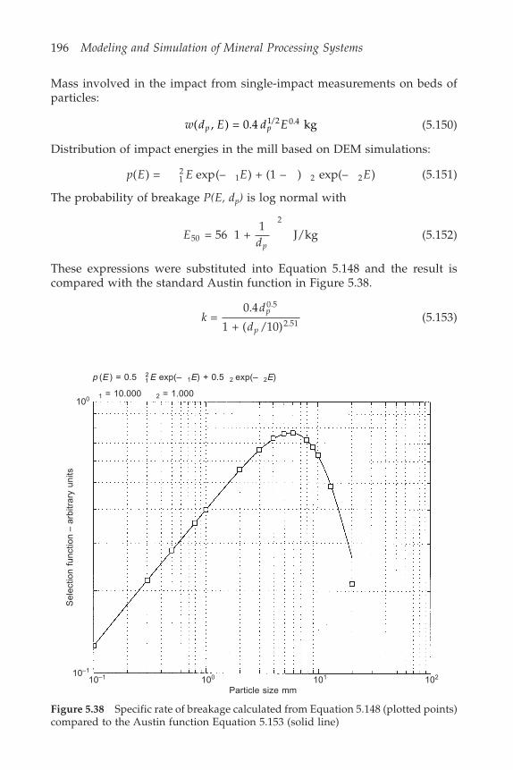
196 Modeling and Simulation of Mineral Processing Systems
Mass involved in the impact from single-impact measurements on beds ofparticles:
w d E d Ep p( , ) = 0.4 kg1/2 0.4 (5.150)
Distribution of impact energies in the mill based on DEM simulations:
p E E E E( ) = exp(– ) + (1 – ) exp(– )12
1 2 2 (5.151)
The probability of breakage P(E, dp) is log normal with
Edp
50
2
= 56 1 + 1
J/kg (5.152)
These expressions were substituted into Equation 5.148 and the result iscompared with the standard Austin function in Figure 5.38.
kd
dp
p =
0.4
1 + ( /10)
0.5
2.51 (5.153)
1 = 10.000 2 = 1.000
p (E ) = 0.5 12 E exp(– 1E) + 0.5 2 exp(– 2E)
100
10–1
10–1 100 101 102
Particle size mm
Sel
ectio
n fu
nctio
n–
arbi
trar
y un
its
Figure 5.38 Specific rate of breakage calculated from Equation 5.148 (plotted points)compared to the Austin function Equation 5.153 (solid line)
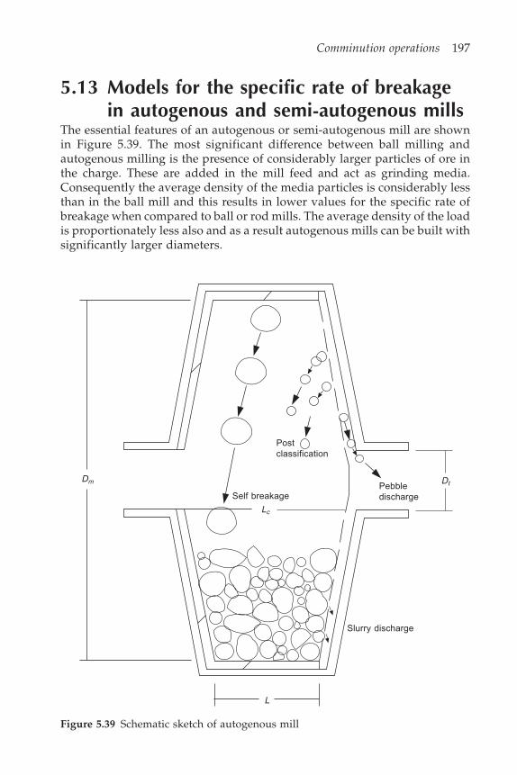
Comminution operations 197
5.13 Models for the specific rate of breakagein autogenous and semi-autogenous mills
The essential features of an autogenous or semi-autogenous mill are shownin Figure 5.39. The most significant difference between ball milling andautogenous milling is the presence of considerably larger particles of ore inthe charge. These are added in the mill feed and act as grinding media.Consequently the average density of the media particles is considerably lessthan in the ball mill and this results in lower values for the specific rate ofbreakage when compared to ball or rod mills. The average density of the loadis proportionately less also and as a result autogenous mills can be built withsignificantly larger diameters.
Figure 5.39 Schematic sketch of autogenous mill
Dm
Lc
Dt
Slurry discharge
L
Self breakage
Postclassification
Pebbledischarge

198 Modeling and Simulation of Mineral Processing Systems
Equation 5.124 defines the size distribution in the charge of an autogenousor semi-autogenous mill using the population balance model. The sizedistribution in the mill discharge can be calculated from the size distributionof the charge using Equation 5.126. In order to use these equations it isnecessary to be able to calculate the selection functions and breakage functionsfor the separate breakage mechanisms that occur in the mill, namely attrition,chipping, impact fracture and self-breakage. Chipping and attrition occur onthe surface of the particle and the inner core of the particle is not affected.Particles are subject to attrition through friction between particles and alsobetween particles and the walls of the mill. Particles are chipped throughimpact against other particles or against the walls of the mills. The sizedistribution of the progeny from attrition is somewhat finer than that fromchipping but these two subprocesses are normally lumped together. Goldmanand Barbery (1988), Goldman et al. (1991) and Austin et al. (1987) have measuredwear rates in comparatively small test mills in batch mode and all the datacan be described by a wear model of the type
i pid = (5.154)
Austin et al. favor = 0 while Goldman et al. (1991) found = 0.37 in a1.75 m diameter pilot plant mill and = 1 in a 0.75 m laboratory mill (Goldmanet al. 1988). The surface specific wear rate depends on the milling environmentdecreasing as the proportion of fines increases in the mill charge and increasingwith mill load and mill diameter. Careful experiments have shown that thesurface specific wear rate on a particular particle decreases for several minutesafter it has been introduced into the mill environment because its initialrough surface is subject to chipping and attrition that decreases as the particlebecomes rounded. Because of this phenomenon the population balance equationshould also allow for a distribution of sojourn times of the particles in themill. This level of fine detail is not justified at the level of modeling that isdescribed here.
The value of the specific attrition rate is ore specific and should bemeasured experimentally for the ore. An attrition method has been developedat Julius Kruttschnitt Mineral Research Center and is described in their 25th
anniversary volume (Napier-Munn et al., 1996). A sample of the material inthe 38 mm to 50 mm size range is tumbled for 10 minutes. The size distributionof the charge after this time is determined by screening and is typicallybimodal as shown in Figure 5.40. Estimates of the specific attrition rate andthe attrition breakage function can be easily obtained from this graph. FromEquation 2.109:
dmdt
x m
xs = –2
= –32+
1– (5.155)
Since the particles do not change much in size during the test, x is a constantequal to df for the duration of the test.
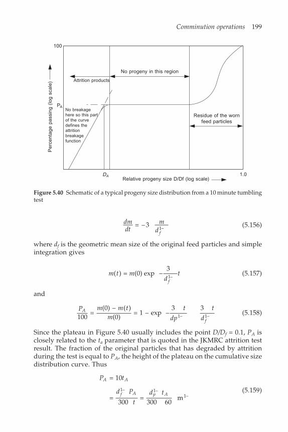
Comminution operations 199
dmdt
md f
= – 3 1– (5.156)
where df is the geometric mean size of the original feed particles and simpleintegration gives
m t md
tf
( ) = (0) exp –31– (5.157)
and
P m m tm
t
dp
t
dA
f100
= (0) – ( )
(0) = 1 – exp –
3 31– 1– (5.158)
Since the plateau in Figure 5.40 usually includes the point D/Df = 0.1, PA isclosely related to the ta parameter that is quoted in the JKMRC attrition testresult. The fraction of the original particles that has degraded by attritionduring the test is equal to PA, the height of the plateau on the cumulative sizedistribution curve. Thus
P t
d P
td t
A A
f A p A
= 10
= 300
= 300 60
m1– 1–
1–(5.159)
Per
cent
age
pass
ing
(log
scal
e)100
PANo breakagehere so this partof the curvedefines theattritionbreakagefunction
Attrition products
No progeny in this region
Residue of the wornfeed particles
DARelative progeny size D/Df (log scale)
1.0
Figure 5.40 Schematic of a typical progeny size distribution from a 10 minute tumblingtest
200 Modeling and Simulation of Mineral Processing Systems
The specific rate of breakage due to impact follows the pattern observed inball mills and the Austin method can be used to model the specific rate ofbreakage due to impact fracture provided that due allowance is made for thelower density of the medium particles. In semi-autogenous mills due allowancemust also be made for the presence of steel balls as well as the autogenousmedia. These effects are modeled by the Austin scale-up procedure by includingthe autogenous medium in the media size classes in Equation 5.133. Howeverthe lower density of the media particles must be allowed for and in Equation5.133 both mk and k must be scaled by the ratio k/ s where k is the densityof media particles in media size class k and s is the density of the balls in thetest mill.
m mk kpebbles steel
pebbles
steel = (5.160)
and
k kpebbles steel
pebbles
steel = (5.161)
The sharp decrease in the specific rate of breakage that is evident for particlesthat are too large to be properly nipped during an impact event is especiallyimportant in autogenous and semi-autogenous mills because the coarse feedsupplies many particles in this size range. An intermediate size range existsin the autogenous mill in which the particles are too large to suffer impactbreakage but are too small to suffer self-breakage. Particles in this size rangecan accumulate in the mill because they neither break nor are they dischargedunless appropriate ports are provided in the discharge grate. This is thephenomenon of critical size build up.
The phenomenon of self-breakage is completely absent in ball mills but itplays an important role in autogenous milling. The larger the particle and thegreater its height of fall in the mill, the larger its probability of self-breakageon impact. Particles smaller than 10 mm or so have negligible breakageprobabilities and consequently very low values of the specific rate of self-breakage. Specific rates of breakage by impact fracture and self-breakage areadditive and the variation of ki with particle size over the entire size range isshown schematically in Figure 5.41. The overall model is obtained fromEquations 5.127 and 5.7.
kS d
dG
E Ei
p
p E =
1 + ( / ) + drop frequency
ln( / )1 50 (5.162)
In Equation 5.162, E is the average kinetic energy per unit mass of a lump ofsize dp when it impacts the liner or the charge after being released at the topof the mill during tumbling. This is calculated as the potential energy of theparticle at a fraction of the inside diameter of the mill. E50 is the medianparticle fracture energy of a lump of size dp. For larger lumps this is independent
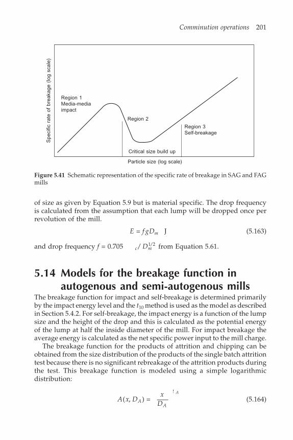
Comminution operations 201
of size as given by Equation 5.9 but is material specific. The drop frequencyis calculated from the assumption that each lump will be dropped once perrevolution of the mill.
E = f gDm J (5.163)
and drop frequency f = 0.705 c/ Dm1/2 from Equation 5.61.
5.14 Models for the breakage function inautogenous and semi-autogenous mills
The breakage function for impact and self-breakage is determined primarilyby the impact energy level and the t10 method is used as the model as describedin Section 5.4.2. For self-breakage, the impact energy is a function of the lumpsize and the height of the drop and this is calculated as the potential energyof the lump at half the inside diameter of the mill. For impact breakage theaverage energy is calculated as the net specific power input to the mill charge.
The breakage function for the products of attrition and chipping can beobtained from the size distribution of the products of the single batch attritiontest because there is no significant rebreakage of the attrition products duringthe test. This breakage function is modeled using a simple logarithmicdistribution:
A x Dx
DAA
A
( , ) = !
(5.164)
Spe
cific
rat
e of
bre
akag
e (lo
g sc
ale)
Region 1Media-mediaimpact
Region 2
Critical size build up
Region 3Self-breakage
Particle size (log scale)
Figure 5.41 Schematic representation of the specific rate of breakage in SAG and FAGmills
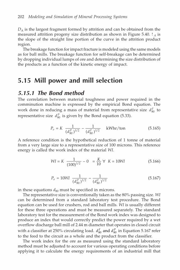
202 Modeling and Simulation of Mineral Processing Systems
DA is the largest fragment formed by attrition and can be obtained from themeasured attrition progeny size distribution as shown in Figure 5.40. ! A isthe slope of the straight line portion of the curve in the attrition productregion.
The breakage function for impact fracture is modeled using the same modelsas for ball mills. The breakage function for self-breakage can be determinedby dropping individual lumps of ore and determining the size distribution ofthe products as a function of the kinetic energy of impact.
5.15 Mill power and mill selection
5.15.1 The Bond methodThe correlation between material toughness and power required in thecomminution machine is expressed by the empirical Bond equation. Thework done in reducing a mass of material from representative size d F
80 torepresentative size d P
80 is given by the Bond equation (5.33).
P Kd d
o P F = 1
( )– 1
( ) kWhr/ton
801/2
801/2
(5.165)
A reference condition is the hypothetical reduction of 1 tonne of materialfrom a very large size to a representative size of 100 microns. This referenceenergy is called the work index of the material WI.
WI K K K WI = 1(100)
– 0 = 10
= 101/2
∀ (5.166)
P WId d
o P F = 10 1
( )– 1
( )801/2
801/2
(5.167)
in these equations d80 must be specified in microns.The representative size is conventionally taken as the 80% passing size. WI
can be determined from a standard laboratory test procedure. The Bondequation can be used for crushers, rod and ball mills. WI is usually differentfor these three operations and must be measured separately. The standardlaboratory test for the measurement of the Bond work index was designed toproduce an index that would correctly predict the power required by a wetoverflow discharge ball mill of 2.44 m diameter that operates in closed circuitwith a classifier at 250% circulating load. d dF P
80 80 and in Equation 5.167 referto the feed to the circuit as a whole and the product from the classifier.
The work index for the ore as measured using the standard laboratorymethod must be adjusted to account for various operating conditions beforeapplying it to calculate the energy requirements of an industrial mill that
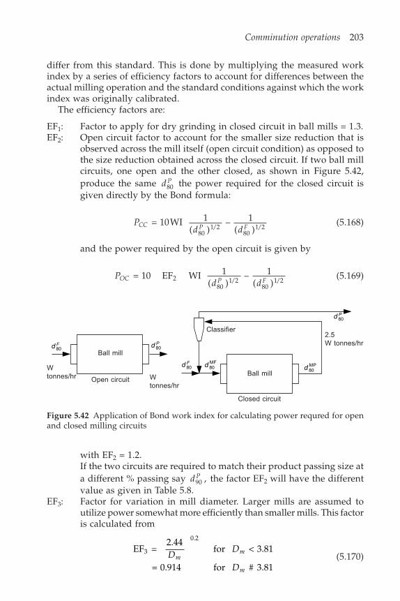
Comminution operations 203
differ from this standard. This is done by multiplying the measured workindex by a series of efficiency factors to account for differences between theactual milling operation and the standard conditions against which the workindex was originally calibrated.
The efficiency factors are:
EF1: Factor to apply for dry grinding in closed circuit in ball mills = 1.3.EF2: Open circuit factor to account for the smaller size reduction that is
observed across the mill itself (open circuit condition) as opposed tothe size reduction obtained across the closed circuit. If two ball millcircuits, one open and the other closed, as shown in Figure 5.42,produce the same d P
80 the power required for the closed circuit isgiven directly by the Bond formula:
Pd d
CC P F = 10WI 1
( )– 1
( )801/2
801/2 (5.168)
and the power required by the open circuit is given by
Pd d
OC P F = 10 EF WI 1
( )– 1
( )2
801/2
801/2 (5.169)
Wtonnes/hr
Ball mill
Wtonnes/hr
Ball mill
Closed circuit
2.5W tonnes/hr
Classifier
Open circuit
d 80MF
d 80MP
Figure 5.42 Application of Bond work index for calculating power requred for openand closed milling circuits
with EF2 = 1.2.If the two circuits are required to match their product passing size ata different % passing say d P
90 , the factor EF2 will have the differentvalue as given in Table 5.8.
EF3: Factor for variation in mill diameter. Larger mills are assumed toutilize power somewhat more efficiently than smaller mills. This factoris calculated from
EF = 2.44
for < 3.81
= 0.914 for 3.81
3
0.2
DD
Dm
m
m #(5.170)
d F80
d P80
d F80
d P80
204 Modeling and Simulation of Mineral Processing Systems
EF4: Oversize feed factor. The optimal d F80 size for a ball mill that grinds
material having a work index of WI kW hr/tonne is given by
FO = 4 14.3WI
mm1/2
(5.171)
When the feed has a size distribution coarser than the optimum, themill must draw more power to achieve the desired product size. Theappropriate efficiency factor is given by
EF = 1 + (WI – 7)( – )
480d F
R F
Fo
r o(5.172)
where Rr is the reduction ratio d
d
F
P80
80
EF5: The work index in a ball mill increases when the reduction ratiodecreases below 3 and the efficiency factor is given by
EF = 1 + 0.013– 1.355 Rr
(5.173)
To size a ball mill or rod mill that must process W tonnes/hr it is necessaryto calculate the mill power required from
P = Po W (5.174)
and find a mill from the manufacturer’s catalogue that can accept that power.If manufacturer’s data is not available, Equations 5.65 or 5.67 can be used toselect a suitable mill. This will not produce a unique design for the millbecause many combinations of Dm and L will satisfy these equations and theaspect ratio of the mill must be chosen to ensure that the mill will providesufficient residence time or specific power input to produce the requiredproduct size distribution as calculated from Equation 5.84 or 5.126. It isimportant to note that the geometry of the mill will determine the power
Table 5.8 Bond work index efficiency factor for wet opencircuit milling
Reference % passing Open circuit efficiency factor EF2
50% 1.03560% 1.0570% 1.1080% 1.2090% 1.4092% 1.4695% 1.5798% 1.70
Comminution operations 205
input not the tonnage through the mill. The power consumed will give acertain amount of size reduction and the output size will be a function of thetonnage. By contrast a crusher will produce a fixed size reduction ratio andthe power will vary to match the tonnage subject to the maximum poweravailable from the motor that is installed on the crusher.
5.16 The batch mill
5.16.1 Batch grinding of homogeneous solidsThe comminution properties of materials are often determined in the laboratoryby following the size distribution during milling in a batch mill. In such atest, the mill is charged with a given mass of feed material and the mill isoperated without continuous discharge and feed.
The size distribution in the charge in a batch mill changes continuouslywith time. The mass balance must be written for each size class.
For the top size:
Mdmdt
k Mm11 1 = – (5.175)
It is usually adequate to assume that k1 does not vary with time and thisequation can be easily integrated to give
m m e k t1 1
– = (0) 1 (5.176)
This solution plots as a straight line on log-linear coordinates.For the next size down:
Mdm
dtk Mm k Mm b2
2 2 1 1 21 = – + (5.177)
dmdt
k m k b m k b m e k t22 2 1 21 1 1 21 1
– + = = (0) 1 (5.178)
This is a first order linear differential equation which has a solution of theform:
m Ae Bek t k t2
– – = + 2 1 (5.179)
where A and B are constants that must be determined from the differentialequation and from the initial conditions. First the proposed solution isdifferentiated
dmdt
Ak e Bk ek t k t22
–1
– = – –2 1 (5.180)
These expressions for w2 and its derivative are substituted into the originaldifferential equation

206 Modeling and Simulation of Mineral Processing Systems
– – + + = 2 1–
2–
2–
1 21 1–2 1 2 1 1Ak e Bk e k Ae k Be k b m ek t k t k t k t k t( )0 (5.181)
which simplifies to
(– + ) = (0)1 2–
1 21 1–1 1k B k B e k b m ek t k t (5.182)
so that B is given by
Bk b m
k k =
–1 21 1
2 1
( )0(5.183)
A must be evaluated from the initial condition.
m2(0) = A + B (5.184)
which gives
A = m2(0) – B (5.185)
and
m m e B e e
m ek b m
k ke e
k t k t k t
k t k t k t
2 2– – –
2– 1 21 1
2 1
– –
= (0) – ( – )
= (0) –(0)
–( – )
2 2 1
2 2 1(5.186)
The solution can be continued in this way to develop the solution from sizeto size. The solution is tedious but not impossible. It is better to develop asolution that works automatically for all sizes and which is especially suitedto computer methods. Note firstly that a general solution can take two forms:
m e
m m
i j
i
ijk t
i j
i
ij j
j =
= (0)
=1
–
=1
(5.187)
The coefficients ij are not functions of time but are functions of the initialconditions and the coefficients ij are not functions of the initial conditionsbut they vary with the time. The coefficients ij can be developed throughsome recursion relationships as follows:
The differential equation that describes the variation of each of the sizeclasses is
dmdt
k m b k mii i j
i
ij j j = – + =1
–1
(5.188)
The general solution is now substituted into this equation
j
i
ij jk t
i j
i
ijk t
j
i
ij jl
j
jlk tk e k e b k ej j l
=1 =1
–
=1
–1
=1–– = – + (5.189)
Re-arranging and collecting terms

Comminution operations 207
j
i
ij i jk t
j
i
l
j
ij j jlk tk k e b k ej l
=1
–
=1
–1
=1– ( – ) = (5.190)
The order of the double summation must now be reversed
l
i
il i lk t
l
i
j l
i
ij j jlk tk k e b k el l
=1
–1–
=1
–1
=
–1– ( – ) = (5.191)
The change in the limits on the double summation should be noted particularly.The region over which the double summation operates must not change asthe order of summation is switched.
Now the terms are collected
l
i
il i l j l
i
ij j jlk tk k b k e l
=1
–1
=
–1– ( – ) – = 0 (5.192)
The coefficient of each exponential must be zero if the summation is to bezero for every value of t,
il i l j l
i
ij j jlk k b k( – ) = =
–1
(5.193)
which provides the value of each value of except for ∃ii.
ili l j l
i
ij j jlk kb k i l = 1
– for >
=
–1
(5.194)
ii can be obtained from the initial condition
mi j
i
ij ii j
i
ij(0) = = + =1 =1
–1
(5.195)
ii ij l
i
ijm= (0) –=
–1
(5.196)
All the coefficients can be solved by recursion starting from i = 1.
11 1
212 1
21 1 11
= (0)
= 1–
m
k kb k (5.197)
etc.This recursion is most useful in the form
ij = cij aj with j < i and cii = 1 (5.198)
il il li l j l
i
ij j jl l
ili l j l
i
ij j jl
c ak k
b k c a
ck k
b k c
= = 1–
= 1–
=
–1
=
–1(5.199)
208 Modeling and Simulation of Mineral Processing Systems
ii i i j
i
ij ja m c a = = (0) –=1
–1
(5.200)
Then the cil’s are independent of both the time and the initial conditions andthey can be calculated once and for all from a knowledge of the specificbreakage rate constants and the breakage function.
5.16.2 Batch grinding of heterogeneous solidsThe batch comminution equation for heterogeneous solids is
dpdt
k p k b pij
ij ijl
j
k K
K
kl ijkl kll
l
= – + =1
–1
= *
**
(5.201)
In Equation 5.201 i, j, k and l index the parent particle composition, the parentsize, the progeny composition and the progeny size respectively. K Kl l* and **
are the left and right hand boundaries of region R in the Andrews-Mikadiagram for parent particles in size class l. bijkl is the discretized version of thefunction b(g, dp|g , dp ).
In practice it is convenient to decouple the size reduction process from theliberation process. This can be done by using the conditional breakage functions:
bij kl = bj ,kl bi, j kl (5.202)
where bj ,kl is the fraction of material breaking from class k, l that reports tosize class j. bi, jkl is the conditional transfer coefficient from grade class k tograde class i given that the particle transfers from size class l to size class j.bi,jk l is usually represented as an Andrews-Mika diagram as described inChapter 3. bj,kl is referred to as the ‘size breakage function’ and bi,jkl as theAndrews-Mika coefficients. Equation 5.202 is completely general and doesnot depend on the assumption of random fracture. bj, kl and bi,j kl are conditionaldistributions and must satisfy the conditions
j l
N
j klb= +1 , = 1 (5.203)
and
i i jklb=1
12
, = 1 (5.204)
Appropriate models for the Andrews-Mika diagram are discussed inChapter 3.
A solution to the heterogeneous batch comminution equation can begenerated by exploiting the linearity of the differential equations to generatethe general solution
p eijl
j
k ijklk tkl =
=1 =1
12– (5.205)

Comminution operations 209
The coefficients in Equation 5.205 are related to the selection and breakagefunctions and to the initial conditions using the following recursionrelationships
ijmj = 0 if i %m (5.206)
ijij ijl
j
k ijklp = (0) – =1
–1
=1
12
(5.207)
ijmnl n
j
k kl ijkl klmn
ij mn
k b
k k =
–=
–1
=1
12
(5.208)
Note that the summations in Equation 5.208 run over the feeder regions andnot over the attainable regions.
This solution to Equation 5.201 is based on the usual convention thatbreakage implies that all progeny leave the size class of the parent particle.The pathological case kij = kmn is occasionally encountered in practice. Whenit occurs, it is usually handled by making a slight adjustment to the parametersthat define the relationship between the specific rate of breakage and theparticle size to assure that no two values of kij are exactly equal.
Equation 5.205 represents a complete and convenient solution to the discreteversion of the batch comminution equation with liberation and this solutionproduces the size distribution as well as the liberation distribution as a functionof the time of grinding.
BibliographyThe bibliography dealing with comminution is large. The classic referencefor the application of population balance methods is Austin et al. (1984). Thisbook discusses the application of the population balance method and describesthe careful experimental work that is required to measure the breakage andselection functions, which are central to the method, in the laboratory. Theconsiderable work done at the Julius Kruttschnitt Mineral Research Centreon the application of these models to simulation and plant evaluation arerecorded in two important texts by Lynch (1977) and by Napier-Munn et al.(1996). Useful research material on comminution can be found in two specialissues of the International Journal of Mineral Processing, Volume 22, 1988 andcombined Volumes 44 and 45, 1996.
Many good texts on fracture mechanics are available. A modern text thatcovers the material that is used here is Anderson (1995). Lawn (1993) gives anexcellent account of the fracture of brittle solids.
Bearman et al. (1989), Middlemiss (1989) and Middlemiss and Tait (1990)have measured the fracture toughness of some minerals and ores.
Elementary breakage events have been studied in the laboratory using thedrop weight method on beds of particles (Höffler, 1990; Bourgeois, 1993) and
210 Modeling and Simulation of Mineral Processing Systems
by slow compression of constrained particle beds in a piston and dieconfiguration (Liu and Schönert, 1996; Fandrich et al., 1997).
The concept of particle fracture energy was introduced by Baumgardt et al.in 1975. A method for the accurate measurement of this particle propertyusing the fast load cell is described by Tavares and King (1998).
The t10 method for reconstructing the breakage function was developed byNarayanan and Whiten (1983) using data originally obtained using thependulum impact test.
The models for the gyratory and jaw crushers is based on data from theNordberg Reference Manual, Nordberg Inc., 4th edition 1993. Use of thelogarithmic distribution for plant simulation and optimization was reportedby Csoke et al. (1996).
The model used for cone crushers is based on Whiten et al. (1979), Whiten(1973) and Karra (1982).
The use of the energy-specific selection function to scale up ball milloperations is described in Herbst and Fuerstenau (1980), Herbst et al. (1986)and Lo and Herbst (1986, 1988).
Residence-time distributions for the solids in the mill have been measuredby Kinneberg and Herbst (1984) and by Schneider (1995).
The population balance model for the autogenous and semi-autogenousmill is based on the analysis of Hoyer and Austin (1985). Details of the breakagemechanisms in these mills were investigated by Stanley (1974), Austin et al.(1987), Goldman and Barbery (1988), Goldman et al. (1991) and Leung et al.(1988).
Application of the classical Bond method is described by Rowland (1998).The analysis of the batch mill with liberation is described in King and
Schneider (1998).
ReferencesAnderson, T.L. (1995) Fracture Mechanics. 2nd edition, CRC Press, p. 47.Austin, L.G. (1990) A mill power equation for SAG mills. Minerals and Metallurgical
Processing, pp. 57–62.Austin, L.G., Klimpel, R.R. and Luckie, P.T. (1984) Process Engineering of Size Reduction:
Ball Milling. Soc. Mining Engineers, New York.Austin, L.G., Menacho, J.M. and Pearcy, F. (1987) Proc. 20th Int. Symposium on the
Application of Computers and Mathematics in the Mineral Industries. S. Afr. Inst. Min.Metall., Johannesburg, pp. 107–126.
Baumgardt, S., Buss, B., May, P. and Schubert, H. (1975) On the comparison of resultsin single grain crushing under different kinds of load. Proc. 11th Intl Mineral ProcessingCongress, pp. 3–32.
Bond, F.C. (1952) The third theory of grinding. Trans. AIME, Vol. 193, pp. 484–494.Bourgeois, F. (1993) Microscale Modeling of Comminution Processes. Ph.D Thesis,
University of Utah.Bearman, R.A., Pine, R.J. and Wills, B.A. (1989) Use of fracture toughness testing in
characterising the comminution potential of rock. Proc. Joint MMIJ/IMM Symposium,Kyoto.
Comminution operations 211
Csoke, B., Petho, S., Foldesi, J. and Meszaros, L. (1996) Optimization of stone-quarrytechnologies. International Journal of Mineral Processing, Vol. 44–45, pp. 447–459.
Dan, C.C. and Schubert, H. (1990) Breakage probability, progeny size distribution andenergy utilization of comminution by impact. Proc. 7th European Symposium onComminution, Conkarjev Dom, Ljubljana 1 : 160–179.
Fandrich, R.G., Bearman, R.A., Boland, J. and Lim, W. (1997) Mineral liberation byparticle bed breakage. Minerals Engineering, Vol. 10, pp. 175–187.
Goldman, M. and Barbery, G. (1988) Wear and chipping of coarse particles in autogenousgrinding: experimental investigation and modeling. Minerals Engineering, Vol. 1,pp. 67–76.
Goldman, M., Barbery, G. and Flament, F. (1991) Modelling load and product distributionin autogenous and semi-autogenous mills: pilot plant tests. CIM Bulletin, Vol. 8(Feb.), pp. 80–86.
Herbst, J.A. and Fuerstenau, D.W. (1980) Scale-up procedure for continuous grindingmill design using population balance models. Int. Jnl Mineral Processing, Vol. 7, pp.1–31.
Herbst, J.A., Lo, Y.C. and Rajamani, K. (1986) Population balance model predictions ofthe performance of large-diameter mills. Minerals and Metallurgical Engineering, pp.114–120.
Höffler, A. (1990) Fundamental Breakage Study of Mineral Particles with an UltrafastLoad Cell Device. Ph.D Thesis, University of Utah.
Hoyer, D.I. and Austin, L.G. (1985) A simulation model for autogenous pebble mills.Preprint number 85-430, SME-AIME Fall Meeting, Albuquerque, Oct.
Karra, V.K. (1982) A process performance model for ore crushers. Proc. 4th Int. Min.Proc. Congress Toronto, Vol. III, pp. 6.1–6.14.
Kick, F. (1883) Dinglers Polytechnisches Journal, Vol. 247, pp. 1–5.King, R.P. and Schneider, C.L. (1998) Mineral liberation and the batch comminution
equation. Minerals Engineering, Vol. 11, pp. 1143–1160.Kinneberg, D.J. and Herbst, J.A. (1984) A comparison of linear and nonlinear models
for open-circuit ball mill grinding. Intl. Jnl Mineral Processing, Vol. 13, pp. 143–165.Lawn, B. (1993) Fracture of Brittle Solids. 2nd edition, Cambridge University Press,
Cambridge.Leung, K., Morrison, R.D. and Whiten, W.J. (1988) An energy based ore-specific model
for autogenous and semi-autogenous grinding. Coper ’87, Universidadde Chile,pp. 71–85.
Liu, J. and Schönert, K. (1996) Modelling of interparticle breakage. Int. Jnl Miner.Processing, Vol. 44–45, pp. 101–115.
Lo Y.C. and Herbst, J.A. (1986) Consideration of ball size effects in the populationbalance approach to mill scale-up. In Advances in Mineral Processing (P. Somasudaran,ed.), Society of Mining Engineers Inc. Littleton, pp. 33–47.
Lo, Y.C. and Herbst, J.A. (1988) Analysis of the performance of large-diameter mills atBougainville using the population balance approach. Minerals and MetallurgicalProcessing, pp. 221–226.
Lynch, A.J. (1977) Mineral Crushing and Grinding Circuits. Their simulation, Optimisation,Design and Control. Elsevier Scientific Publishing Company, Amsterdam.
Menacho, J.M. (1986) Some solutions for the kinetics of combined fracture and abrasionbreakage. Powder Technology, Vol. 49, pp. 87–96.
Middlemiss, S.N. (1989) Effects of notch size and geometry and test techniques onfracture toughness of quartzite. Dept of Metallurgy and Materials Engineering,Univ. of the Witwatersrand. Report FRG/89/5.

212 Modeling and Simulation of Mineral Processing Systems
Middlemiss, S.N. and Tait, R.B. (1990) Fracture toughness of quartzite as a function ofvarious parameters including triaxial confining stress, temperature and underconditions of shear. Univ. of the Witwatersrand, Dept of Metallurgy and MaterialsEngineering Report FRG 90/1.
Morrell, S. (1996) Power draw of wet tumbling mills and its relationship to chargedynamics, Part 2: An empirical approach to modeling of mill power draw. Trans.Instn Mining Metall. (Sect. C: Mineral Processing Extr Metall.), 105, January–April,pp. C54–C62.
Napier-Munn, T.J., Morrell, S., Morrison, R.D. and Kojovic, T. (1996) MineralComminution Circuits. Their Operation and Optimisation. Julius Kruttschnitt MineralResearch Centre, Brisbane.
Narayanan, S.S. and Whiten, W.J. (1983) Breakage characteristics for ores for ball millmodelling. Proc. Australas. Instn Min. Metall., No. 286, pp. 31–39.
Pauw, O.G. and Mare, M.S. (1988) The determination of optimum impact-breakageroutes for an ore. Powder Technology, Vol. 54, pp. 3–13.
Rajamani, R.K., Mishra, B.K., Songfack, P. and Venugopal, R. (1999) Millsoft – simulationsoftware for tumbling-mill design and trouble shooting. Mining Engineering,December, pp. 41–47.
Rittinger, R.P. von, (1857) Lehrbuck der Aufbereitungskunde, Ernst u. Korn, Berlin.Rowland, C.A. (1998) Using the Bond work index to measure the operating comminution
efficiency. Minerals & Metallurgical Processing, Vol. 15, pp. 32–36.Rowland, C.A. and Kjos, D.M. (1980) Rod and Ball Mills. In Mineral Processing Plant
Design, 2nd edition (A.L. Mular and R.B. Bhappu, eds), SME Littleton, CO, p. 239.Schneider, C.L. (1995) The Measurement and Calculation of Liberation in Continuous
grinding Circuits, Ph.D Thesis, University of Utah.Stanley, G.G. (1974) Mechanisms in the autogenous mill and their mathematical
representation. S. Afr. Inst. Mining Metall., Vol. 75, pp. 77–98.Tavares, L.M. and King, R.P. (1998) Single-particle fracture under impact loading. Intl
Journal Mineral Processing, Vol. 54, pp. 1–28.Whiten, W.J., Walter, G.W. and White, M.E. (1979) A breakage function suitable for
crusher models. 4th Tewkesbury Symposium, Melbourne, pp. 19.1–19.3.Whiten, W.J. (1973) The simulation of crushing plants. Application of computer methods
in the mineral industry. Apcom 10, S. Afr. Inst. of Mining and Metall., Johannesburg,pp. 317–323.
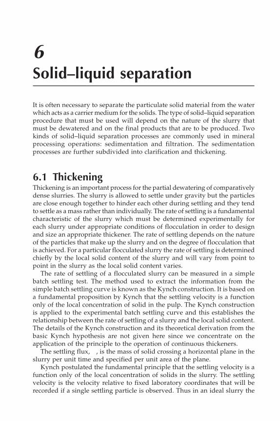
6Solid–liquid separation
It is often necessary to separate the particulate solid material from the waterwhich acts as a carrier medium for the solids. The type of solid–liquid separationprocedure that must be used will depend on the nature of the slurry thatmust be dewatered and on the final products that are to be produced. Twokinds of solid–liquid separation processes are commonly used in mineralprocessing operations: sedimentation and filtration. The sedimentationprocesses are further subdivided into clarification and thickening.
6.1 ThickeningThickening is an important process for the partial dewatering of comparativelydense slurries. The slurry is allowed to settle under gravity but the particlesare close enough together to hinder each other during settling and they tendto settle as a mass rather than individually. The rate of settling is a fundamentalcharacteristic of the slurry which must be determined experimentally foreach slurry under appropriate conditions of flocculation in order to designand size an appropriate thickener. The rate of settling depends on the natureof the particles that make up the slurry and on the degree of flocculation thatis achieved. For a particular flocculated slurry the rate of settling is determinedchiefly by the local solid content of the slurry and will vary from point topoint in the slurry as the local solid content varies.
The rate of settling of a flocculated slurry can be measured in a simplebatch settling test. The method used to extract the information from thesimple batch settling curve is known as the Kynch construction. It is based ona fundamental proposition by Kynch that the settling velocity is a functiononly of the local concentration of solid in the pulp. The Kynch constructionis applied to the experimental batch settling curve and this establishes therelationship between the rate of settling of a slurry and the local solid content.The details of the Kynch construction and its theoretical derivation from thebasic Kynch hypothesis are not given here since we concentrate on theapplication of the principle to the operation of continuous thickeners.
The settling flux, , is the mass of solid crossing a horizontal plane in theslurry per unit time and specified per unit area of the plane.
Kynch postulated the fundamental principle that the settling velocity is afunction only of the local concentration of solids in the slurry. The settlingvelocity is the velocity relative to fixed laboratory coordinates that will berecorded if a single settling particle is observed. Thus in an ideal slurry the
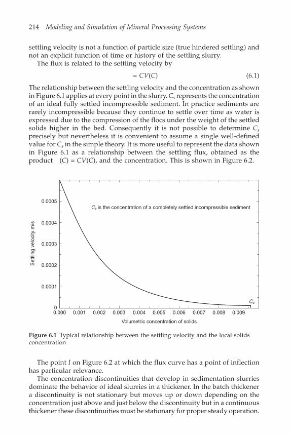
214 Modeling and Simulation of Mineral Processing Systems
0.0005
0.0004
0.0003
0.0002
0.0001
00.000 0.001 0.002 0.003 0.004 0.005 0.006 0.007 0.008 0.009
Cs
Cs is the concentration of a completely settled incompressible sediment
Volumetric concentration of solids
Set
tling
vel
ocity
m/s
settling velocity is not a function of particle size (true hindered settling) andnot an explicit function of time or history of the settling slurry.
The flux is related to the settling velocity by
= CV(C) (6.1)
The relationship between the settling velocity and the concentration as shownin Figure 6.1 applies at every point in the slurry. Cs represents the concentrationof an ideal fully settled incompressible sediment. In practice sediments arerarely incompressible because they continue to settle over time as water isexpressed due to the compression of the flocs under the weight of the settledsolids higher in the bed. Consequently it is not possible to determine Csprecisely but nevertheless it is convenient to assume a single well-definedvalue for Cs in the simple theory. It is more useful to represent the data shownin Figure 6.1 as a relationship between the settling flux, obtained as theproduct (C) = CV(C), and the concentration. This is shown in Figure 6.2.
Figure 6.1 Typical relationship between the settling velocity and the local solidsconcentration
The point I on Figure 6.2 at which the flux curve has a point of inflectionhas particular relevance.
The concentration discontinuities that develop in sedimentation slurriesdominate the behavior of ideal slurries in a thickener. In the batch thickenera discontinuity is not stationary but moves up or down depending on theconcentration just above and just below the discontinuity but in a continuousthickener these discontinuities must be stationary for proper steady operation.
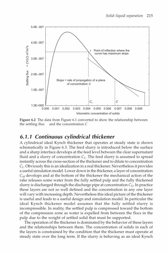
Solid–liquid separation 215
5.0E–007
4.0E–007
3.0E–007
2.0E–007
1.0E–007
1.0E+000
Set
tling
flux
=
CV
(C)
m3 /m
2 s
0.000 0.001 0.002 0.003 0.004 0.005 0.006 0.007 0.008 0.009
CC1
Slope = rate of propogation of a plane of concentration C
I Point of inflection where thecurve has maximum slope
Volumetric concentration of solids
6.1.1 Continuous cylindrical thickenerA cylindrical ideal Kynch thickener that operates at steady state is shownschematically in Figure 6.3. The feed slurry is introduced below the surfaceand a sharp interface develops at the feed level between the clear supernatantfluid and a slurry of concentration CL. The feed slurry is assumed to spreadinstantly across the cross-section of the thickener and to dilute to concentrationCL. Obviously this is an idealization in a real thickener. Nevertheless it providesa useful simulation model. Lower down in the thickener, a layer of concentrationCM develops and at the bottom of the thickener the mechanical action of therake releases some water from the fully settled pulp and the fully thickenedslurry is discharged through the discharge pipe at concentration CD. In practicethese layers are not so well defined and the concentration in any one layerwill vary with increasing depth. Nevertheless this ideal picture of the thickeneris useful and leads to a useful design and simulation model. In particular theideal Kynch thickener model assumes that the fully settled slurry isincompressible. In reality, the settled pulp is compressed toward the bottomof the compression zone as water is expelled from between the flocs in thepulp due to the weight of settled solid that must be supported.
The operation of the thickener is dominated by the behavior of these layersand the relationships between them. The concentration of solids in each ofthe layers is constrained by the condition that the thickener must operate atsteady state over the long term. If the slurry is behaving as an ideal Kynch
Figure 6.2 The data from Figure 6.1 converted to show the relationship betweenthe settling flux and the concentration C

216 Modeling and Simulation of Mineral Processing Systems
slurry, well-defined sharp interfaces will develop in the thickener and theanalysis below shows how these concentrations can be calculated.
The total settling flux relative to fixed coordinates at any level where theconcentration is C must include the effect of the net downward volumetricflow that is due to the removal of pulp at the discharge in addition to thesettling flux of the solid relative to the slurry itself. If the total flux is representedby f(c) and the volumetric flux of slurry below the feed by q then
f(C) = qC + (C) (6.2)
In batch settling q = 0 so that f (C) and (C) are identical. f (C) is plotted fordifferent values of q in Figure 6.4 using the data of Figure 6.1.
Consider any discontinuity as shown in Figure 6.3.Flux of solid into discontinuity from above:
f (C+) = C+q + C+V(C+) (6.3)
Flux of solid leaving from below:
f (C–) = C–q + C–V(C–) (6.4)
In general
f (C+) f (C–) (6.5)
so that solid accumulates at the discontinuity. The accumulation is positive if
f (C+) > f (C–) (6.6)
Figure 6.3 Schematic representation of the ideal Kynch thickener operating at steadystate
Feed slurry at concentration CF
Clear supernatant overflows into discharge trough
Clear supernant liquid
Settling layer at concentration CL
Settling layer concentration CM
Mechanically dewatered layer
Underflow discharged at concentration CD
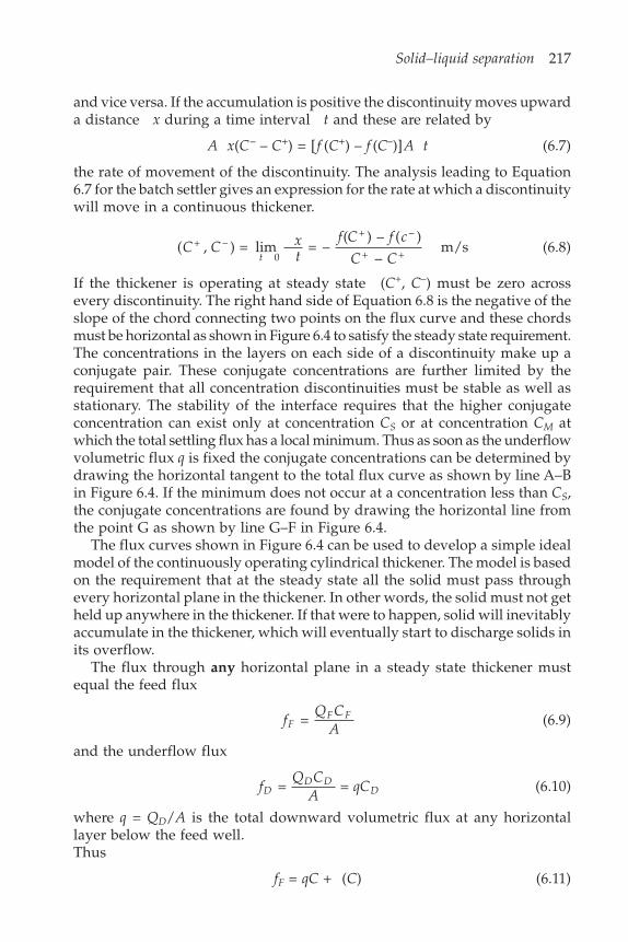
Solid–liquid separation 217
and vice versa. If the accumulation is positive the discontinuity moves upwarda distance x during a time interval t and these are related by
A x(C– – C+) = [ f (C+) – f (C–)]A t (6.7)
the rate of movement of the discontinuity. The analysis leading to Equation6.7 for the batch settler gives an expression for the rate at which a discontinuitywill move in a continuous thickener.
( , ) = lim = –( ) – ( )
– m/s+ –
0
+ –
+ +C C xt
f C f c
C Ct(6.8)
If the thickener is operating at steady state (C+, C–) must be zero acrossevery discontinuity. The right hand side of Equation 6.8 is the negative of theslope of the chord connecting two points on the flux curve and these chordsmust be horizontal as shown in Figure 6.4 to satisfy the steady state requirement.The concentrations in the layers on each side of a discontinuity make up aconjugate pair. These conjugate concentrations are further limited by therequirement that all concentration discontinuities must be stable as well asstationary. The stability of the interface requires that the higher conjugateconcentration can exist only at concentration CS or at concentration CM atwhich the total settling flux has a local minimum. Thus as soon as the underflowvolumetric flux q is fixed the conjugate concentrations can be determined bydrawing the horizontal tangent to the total flux curve as shown by line A–Bin Figure 6.4. If the minimum does not occur at a concentration less than CS,the conjugate concentrations are found by drawing the horizontal line fromthe point G as shown by line G–F in Figure 6.4.
The flux curves shown in Figure 6.4 can be used to develop a simple idealmodel of the continuously operating cylindrical thickener. The model is basedon the requirement that at the steady state all the solid must pass throughevery horizontal plane in the thickener. In other words, the solid must not getheld up anywhere in the thickener. If that were to happen, solid will inevitablyaccumulate in the thickener, which will eventually start to discharge solids inits overflow.
The flux through any horizontal plane in a steady state thickener mustequal the feed flux
fQ C
AFF F = (6.9)
and the underflow flux
fQ C
AqCD
D DD = = (6.10)
where q = QD/A is the total downward volumetric flux at any horizontallayer below the feed well.Thus
fF = qC + (C) (6.11)
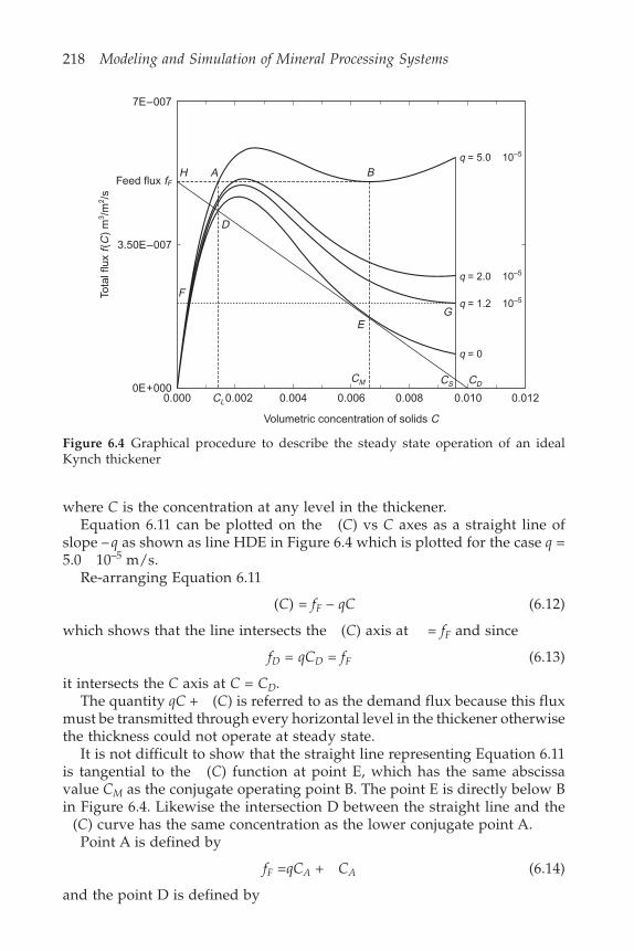
218 Modeling and Simulation of Mineral Processing Systems
where C is the concentration at any level in the thickener.Equation 6.11 can be plotted on the (C) vs C axes as a straight line of
slope – q as shown as line HDE in Figure 6.4 which is plotted for the case q =5.0 10–5 m/s.
Re-arranging Equation 6.11
(C) = fF – qC (6.12)
which shows that the line intersects the (C) axis at = fF and since
fD = qCD = fF (6.13)
it intersects the C axis at C = CD.The quantity qC + (C) is referred to as the demand flux because this flux
must be transmitted through every horizontal level in the thickener otherwisethe thickness could not operate at steady state.
It is not difficult to show that the straight line representing Equation 6.11is tangential to the (C) function at point E, which has the same abscissavalue CM as the conjugate operating point B. The point E is directly below Bin Figure 6.4. Likewise the intersection D between the straight line and the
(C) curve has the same concentration as the lower conjugate point A.Point A is defined by
fF =qCA + CA (6.14)
and the point D is defined by
Figure 6.4 Graphical procedure to describe the steady state operation of an idealKynch thickener
7E–007
Feed flux fF
3.50E–007
0E+0000.000 0.002 0.004 0.006 0.008 0.010 0.012
Volumetric concentration of solids C
CS
Tota
l flu
x f(
C)
m3 /m
2 /s
CDCM
E
B
G
D
AH
F
q = 5.0 10–5
q = 2.0 10–5
q = 1.2 10–5
q = 0
CL

Solid–liquid separation 219
fF – qCD = CD (6.15)
These two equations are true simultaneously only if CD = CA = CL.
6.2 Useful models for the sedimentationvelocity
A number of models have been proposed to relate the sedimentation velocityto the solids concentration and these have been used with varying success todescribe the sedimentation of a variety of slurries that are important in industrialpractice. The most commonly used model is based on the work of Richardsonand Zaki (1954):
V = vTF(1 – rFC)n (6.16)
Here vTF is the terminal settling velocity of an isolated floc and rF is the flocdilution which is the volume of a floc per unit mass of contained solids. Therecommended value for n is 4.65. Scott (1977) has applied this equation to thesedimentation behavior of flocculated Witwatersrand gold ore slurries andsome typical data is compared to this model in Figure 6.5 with vTF = 0.778mm/s and rF = 0.973 m3 floc/tonne solid. The following values have beenreported for Kaolin slurries at pH 6.0: vTF = 0.36 mm/s and rF = 40 m3/m3.Shirato et al. (1970) reported the following values for zinc oxide slurries vTF =0.715 mm/s and rF = 200 and for ferric oxide slurries vTF = 6.42 mm/s and rF= 17.
An alternative model has been used by Shirato et al.
V CC
C = (1 – ) exp (– )3
(6.17)
Zinc oxide slurries in the range 0.02 C 0.26 have been described using = 5.7 10–5 mm/s and = 6.59.
Careful experimental work over wide concentration ranges by Wilhelmand Naide (1981) has shown that the settling velocity of flocculated slurriesover restricted concentration ranges follows the power law:
1 = V
aC b (6.18)
Therefore the complete settling velocity concentration relationship follows asimple equation:
vV
C CTF = 1 + + + . . . .1 21 2 (6.19)
with 0 < 1 < 2 < . . . which describes a variety of slurries over wide rangesof C. Value for b range from 1.0 to as high as 10 or more. Usually no more thantwo power-function terms are required in this equation to describe the settlingvelocity over two or more orders of magnitude variation in the concentration.

220 Modeling and Simulation of Mineral Processing Systems
In Equation 6.19, vTF represents the terminal settling velocity of the individualflocs when they are widely separated from each other and settle as singleentities. vTF is quite difficult to measure but its value can be estimated usingthe methods of Section 4.5 if the size and effective density of the individualflocs can be measured.
Experimental data on the settling of coal refuse sludge measured by Wilhelmand Naide and of flocculated quartzite slurries typical of mineral processingoperations are shown in Figure 6.5. Equation 6.19 describes the settling behaviorof these flocculated slurries well and for these data is significantly better thanthe Richardson-Zakai model.
Figure 6.5 Experimental data obtained using the Kynch graphical construction andfitted by the extended Wilhelm-Naide equation
6.3 Simulation of continuous thickeneroperation
A simple simulation model can be constructed for the continuous cylindricalthickener using the ideal Kynch model. If the area of the thickener is givenand the conditions in the feed pulp are known then
Measured settling velocity of coal refuse sludge (Wilhelm and Naide, 1981)Measured settling velocity of coal refuse sludge (Wilhelm and Naide, 1981)Measured settling velocity of coal refuse sludge (Wilhelm and Naide, 1981)Measured settling velocity of quartzite slurry (Scott, 1972)Calculated settling velocity. vT/V = 1 + 40.6(C/1000)0.341 + 960(C/1000)2.73
Calculated settling velocity. vT/V = 1 + 650(C/700)1.58 + 4 104(C/700)5.02 + 105(C/700)9.3
Richardson-Zakai model V = 0.778(1 – 0.973 10–3C)4.65
Measured settling velocity of CaCO3 slurries (Font, 1988)Calculated settling velocity. 2.61/V = 1 + 2.54 10–5C2.38 + 2.7 10–14C5.41
101
100
10–1
10–2
10–3
10–4
10–5
101 2 3 4 5 6 7 8 9102 2 3 4 5 6 7 8 9103
Slurry concentration kg/m3
Set
tling
vel
ocity
mm
/s

Solid–liquid separation 221
fF = QFCF (6.20)
Thus the underflow concentration and the underflow pumping rate is fixedby the slope and abscissa intercept of the line HDE in Figure 6.4. This definesthe flowrate and the composition of the pulp that is passed from the thickeneron to the next unit in the flowsheet.
The maximum possible feed flux is fixed by the slope of the flux curve atthe point of inflexion I .
fM max = (CI) + CI I (6.21)
The method requires that a suitable model be available for the settling flux.This is calculated using settling velocities given by Equations 6.16, 6.17 or6.19.
The Richardson-Zaki model for the sedimentation velocity can be used tobuild a simple but self-consistent simulation model for the ideal Kynchthickener. The maximum feed rate of solid that can be sent to a thickener ofgiven diameter is fixed by the slope of the sedimentation flux curve at thepoint of inflexion. The sedimentation flux is given by Equation 6.1
= vTFC(1 – rFC)n (6.22)
The point of inflexion is at
Cr nI
F = 2
( + 1)(6.23)
and the critical slope at the point of inflexion is given by
ITF
nn nv
nn n n =
( + 1) (( – 1) – 2 ( – 1) )–1 (6.24)
The maximum possible feed flux occurs when the operating line in Figure 6.4is tangential to the flux curve at the critical point of inflexion. Thus
f C CF I I Imax = ( ) –
=4 ( – 1)
( + 1)
–1
+1vr
n nn
TF
F
n
n(6.25)
The maximum possible feed rate of solids to the thickener is
WFmax = s fF maxA kg/s (6.26)
When the thickener is fed at a rate less than the maximum, the concentrationof the underflow can be calculated from the intersection with the horizontalaxis of the operating line that passes through the given feed flux on thevertical axis and which is tangential to the flux curve as shown in Figure 6.4.This requires the solution of a non-linear equation
CC f
CMM F
M =
( ) –( )
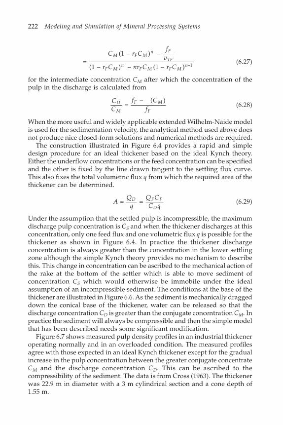
222 Modeling and Simulation of Mineral Processing Systems
=(1 – ) –
(1 – ) – (1 – ) –1
C r Cf
vr C nr C r C
M F Mn F
TF
F Mn
F M F Mn
(6.27)
for the intermediate concentration CM after which the concentration of thepulp in the discharge is calculated from
CC
f Cf
D
M
F M
F =
– ( )(6.28)
When the more useful and widely applicable extended Wilhelm-Naide modelis used for the sedimentation velocity, the analytical method used above doesnot produce nice closed-form solutions and numerical methods are required.
The construction illustrated in Figure 6.4 provides a rapid and simpledesign procedure for an ideal thickener based on the ideal Kynch theory.Either the underflow concentrations or the feed concentration can be specifiedand the other is fixed by the line drawn tangent to the settling flux curve.This also fixes the total volumetric flux q from which the required area of thethickener can be determined.
AQ
qQ CC q
D F F
D = = (6.29)
Under the assumption that the settled pulp is incompressible, the maximumdischarge pulp concentration is CS and when the thickener discharges at thisconcentration, only one feed flux and one volumetric flux q is possible for thethickener as shown in Figure 6.4. In practice the thickener dischargeconcentration is always greater than the concentration in the lower settlingzone although the simple Kynch theory provides no mechanism to describethis. This change in concentration can be ascribed to the mechanical action ofthe rake at the bottom of the settler which is able to move sediment ofconcentration CS which would otherwise be immobile under the idealassumption of an incompressible sediment. The conditions at the base of thethickener are illustrated in Figure 6.6. As the sediment is mechanically draggeddown the conical base of the thickener, water can be released so that thedischarge concentration CD is greater than the conjugate concentration CM. Inpractice the sediment will always be compressible and then the simple modelthat has been described needs some significant modification.
Figure 6.7 shows measured pulp density profiles in an industrial thickeneroperating normally and in an overloaded condition. The measured profilesagree with those expected in an ideal Kynch thickener except for the gradualincrease in the pulp concentration between the greater conjugate concentrateCM and the discharge concentration CD. This can be ascribed to thecompressibility of the sediment. The data is from Cross (1963). The thickenerwas 22.9 m in diameter with a 3 m cylindrical section and a cone depth of1.55 m.
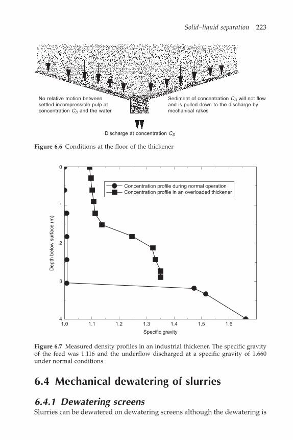
Solid–liquid separation 223
Concentration profile during normal operationConcentration profile in an overloaded thickener
0
1
2
3
4
Dep
th b
elow
sur
face
(m
)
1.0 1.1 1.2 1.3 1.4 1.5 1.6
Specific gravity
6.4 Mechanical dewatering of slurries
6.4.1 Dewatering screensSlurries can be dewatered on dewatering screens although the dewatering is
Discharge at concentration CD
No relative motion betweensettled incompressible pulp atconcentration CD and the water
Sediment of concentration CD will not flowand is pulled down to the discharge bymechanical rakes
Figure 6.6 Conditions at the floor of the thickener
Figure 6.7 Measured density profiles in an industrial thickener. The specific gravityof the feed was 1.116 and the underflow discharged at a specific gravity of 1.660under normal conditions
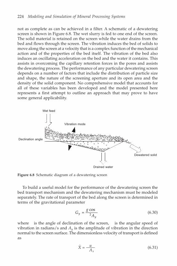
224 Modeling and Simulation of Mineral Processing Systems
not as complete as can be achieved in a filter. A schematic of a dewateringscreen is shown in Figure 6.8. The wet slurry is fed to one end of the screen.The solid material is retained on the screen while the water drains from thebed and flows through the screen. The vibration induces the bed of solids tomove along the screen at a velocity that is a complex function of the mechanicalaction and of the properties of the bed itself. The vibration of the bed alsoinduces an oscillating acceleration on the bed and the water it contains. Thisassists in overcoming the capillary retention forces in the pores and assiststhe dewatering process. The performance of any particular dewatering screendepends on a number of factors that include the distribution of particle sizeand shape, the nature of the screening aperture and its open area and thedensity of the solid component. No comprehensive model that accounts forall of these variables has been developed and the model presented hererepresents a first attempt to outline an approach that may prove to havesome general applicability.
Wet feed
Vibration mode
Declination angle
Drained water
Dewatered solid
Figure 6.8 Schematic diagram of a dewatering screen
To build a useful model for the performance of the dewatering screen thebed transport mechanism and the dewatering mechanism must be modeledseparately. The rate of transport of the bed along the screen is determined interms of the gravitational parameter
Gg
Ay
y =
cos2
(6.30)
where is the angle of declination of the screen, is the angular speed ofvibration in radians/s and Ay is the amplitude of vibration in the directionnormal to the screen surface. The dimensionless velocity of transport is definedas
X uAx
= (6.31)

Solid–liquid separation 225
where u is the velocity of travel along the screen and Ax is the amplitude ofthe vibration in the direction parallel to the screen surface.
A useful model for mineral slurries is
X = a exp(– bGy) (6.32)
The parameter b varies linearly with the slope of the screen
b = 1.44 – 2.32 (6.33)
and parameter a is specific to the material. Ng et al. (1986) have measured a= 1.87 for a coal slurry having d80 = 7.2 mm and d50 = 3.2 mm with a feedwater content of 11%. Unfortunately not much is known about the variationof this parameter with material type and values for other materials are notavailable. The amount of dewatering depends primarily on the time that theslurry spends on the screen, which is fixed by the velocity of travel and thelength of the screen
t Lu
= (6.34)
The dewatering process is governed by the inertial effects that result from therapid acceleration and deceleration of the material on the screen and by therequirement that the draining water must be able to leave the bottom of thescreen by drip dislodgement. Complete dewatering is not possible and theminimum achievable moisture content is a function of several physicalproperties of the particle bed and also of the vibration mechanism. Thisminimum is referred to as the saturation moisture content. If S representsthe saturation moisture content of the bed expressed as mass fraction ofwater in the material, the rate of dewatering can be described by the equation
dSdt
S S = – ( – ) (6.35)
This equation can be integrated to give the saturation as a function of time
S – S = pt–q (6.36)
with
q = 1– 1
(6.37)
and
p = ( ( – 1))–q (6.38)
Combining Equations 6.34 and 6.36 gives the water content of the dischargedslurry as
S S p Lu
q
= + –
(6.39)
226 Modeling and Simulation of Mineral Processing Systems
Ng (1990) has measured p and q for a coal slurry. p is a function of the solidsto be dewatered but is apparently independent of the amplitude, frequencyand mesh size of the screen. q increases with the mesh size of the screenreflecting the greater water discharge rate through the larger mesh. Theirdata give p = 0.234 and
q = 0.33 + 0.081(h – 1.0) (6.40)
where h is the screen mesh size in mm.Particles that are smaller than the mesh size can report to the underflow in
proportion to the recovery of water.The carrying capacity of the dewatering screen can be calculated
approximately from
W = W (1 – e–4h) (6.41)
where W /b is the capacity per unit width of screen at large mesh size. Thislimiting capacity is a function of the size consist of the feed slurry
W d dF F = 20 + 2.5 tonne/hr m for < 12 mm80 80
= 50 + 0.3 tonne/hr m for > 12 mm80 80d dF F (6.42)
Illustrative example 6.1Calculate the water content of a coal slurry after dewatering on a 0.6 mmmesh screen 3.66 m long by 0.914 m wide with angle of declination of 15o.Vibration mode has amplitude 2 cm at a frequency of 300 rpm and is inclinedat 45 to the surface of the screen. The saturation water content of the coal is7.35%.
= 30060
2 = 31.42
Gy = 9.81 cos 1531.42 0.02 sin 45
= 0.6792
b = 1.44 – 2.52 0.262 = 0.780
X = 1.87 exp(–0.780 0.679) = 1.101
Ax = 0.02 cos 45 = 0.014 m
u = 1.101 31.42 0.014 = 0.489 m/s
t = 3.660.489
= 7.485
p = 0.234 q = 0.33 + 0.081(0.6 – 1) = 0.298
Solid–liquid separation 227
The water content of the solid leaving the end of the dewatering screen canbe calculated from Equation 6.39.
S = 0.0735 + 0.234 (7.485)–0.298 = 0.202 kg water/kg slurry
6.5 FiltrationFiltration is used for dewatering operations in mineral processing plants butit is often something of a bottleneck. As a result, alternative processing routesthat avoid filtration are usually preferred. When filtration is used fordewatering, continuous vacuum filters are usually used. These filters areavailable as rotary drums, rotary disks and horizontal belt filters. Of thesethe rotary drum vacuum filter is the most widely used and a simple analysisof these filters is given here.
Generally the rate of flow of filtrate through a filter cake is sufficientlyslow to make the Kozeny-Carman equation a valid descriptor of the process.
Px
Vd
s
p =
150(1 – )2
3 2 (6.43)
which relates the flowrate of filtrate through the cake to the pressure gradient.In Equation 6.43:Vs = superficial liquid velocity,
= filter cake porosity,dp = surface specific particle diameter which, for spherical particles, is related
to the particle specific area per unit volume S0 by dp = 6/S0.If Ac is the interstitial cross-sectional area of the filter cake and L its thickness,Equation 6.43 can be written:
PAL
SQc =
4.17(1 – )202
2 (6.44)
where Q is the volumetric flowrate of filtrate passing through the cake underthe influence of the pressure gradient. The constant 4.17 in Equation 6.44varies with the properties of the particles that make up the filter cake and asimplified form of the equation, called Darcy’s law for porous media, isnormally used
PAL
QK
C = (6.45)
where
KS
= 4.17 (1 – )
2
202 (6.46)
is the permeability of the filter cake.

228 Modeling and Simulation of Mineral Processing Systems
It is convenient to work with the resistance of the bed R = L/Kand Darcy’s law is written
PQRAc
= (6.47)
The thickness of the cake can be related to the mass of solid in the cake perunit area Mc
Mc = s(1 – ) x (6.48)
and the resistance of the cake is related to Mc by
R = Mc (6.49)
is called the specific cake resistance.Usually the resistance of the filter medium contributes a noticeable amount
to the total resistance and it is necessary to add an equivalent resistance ofthe filter cloth or filter medium so that
R = Rcake + Rmedium (6.50)
The medium resistance may not remain constant during the filtration becausesolids may penetrate into the medium and increase the resistance to the flowof filtrate. This effect is neglected here.
P P P QMA
RAc M
c
c
m
c = + = + (6.51)
In a simple batch filtration experiment
QdVdt
f = (6.52)
where Vf is the volume of filtrate passed.The mass of solid deposited in the filter cake is related to the amount of
filtrate collected by
MV C
Acf f
c = (6.53)
where Cs is the concentration of the feed slurry in kg solid/m3 water. Thismakes no allowance for the solids that are in the liquid that is retained by thecake but this is usually negligible in practical applications.
PdVdt A
C V Vf
cs f e = 1 ( + )2
(6.54)
Ve = fictitious volume required to build up a layer of filter cake having thesame resistance as the filter cloth.
This is a two-parameter equation describing batch filtration
Solid–liquid separation 229
A dtdV
kVA
kcf
f
c = + 1 2 (6.55)
which can be integrated at constant pressure to give
tk V
Ak
VA
f
c
f
c =
2 + 1
2
2 2 (6.56)
The constants k1 and k2 can be evaluated from a simple batch filtration test byplotting t/Vf against the filtrate volume Vf.
tV
kA
VkAf c
fc
= 2
+ 12
2 (6.57)
which gives a straight line.Equation 6.56 applies directly to rotary drum filtration since each element
of the drum surface appears as a small batch filter during its sojourn in theslurry. The pressure drop across the cake is constant if the hydrostatic headvariation is neglected. The submergence time is given by
tN
= 2 (6.58)
where N is the rotation speed of the drum in revs/sec and is the submergedangle.
The filtration rate per unit area of drum surface is given by
qVDLf
f =
where D is the diameter of the drum and L its length.
Nk q k qf f = + 21
22
From which the capacity qf can be easily calculated.
Illustrative example 6.2The data given in the table were obtained in a batch filtration test on a singleframe filter press.
The frame was 40 cm by 40 cm. The concentration of solid was 12 kg/m3
water. Viscosity of water = 0.001 Pa s. The pressure drop was held constantat 1.5 105 Pa.
Evaluate the specific cake resistance.
Time s 357 716 1107 1504 1966 2431 2924 3414 3922 4450 4994 5570
Filtrate volumecollected m3 0.02 0.04 0.06 0.08 0.10 0.12 0.14 0.16 0.18 0.20 0.28 0.24
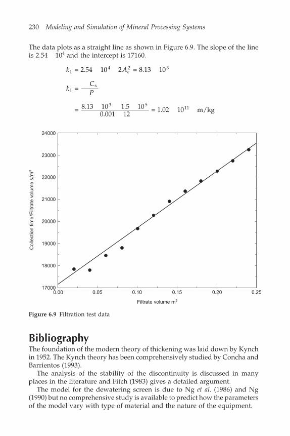
230 Modeling and Simulation of Mineral Processing Systems
24000
23000
22000
21000
20000
19000
18000
170000.00 0.05 0.10 0.15 0.20 0.25
Filtrate volume m3
Col
lect
ion
time
/Filt
rate
vol
ume
s/m
3
Figure 6.9 Filtration test data
The data plots as a straight line as shown in Figure 6.9. The slope of the lineis 2.54 104 and the intercept is 17160.
k Ac14 2 3 = 2.54 10 2 = 8.13 10
kCP1
s =
= 8.13 10 1.5 100.001 12
= 1.02 10 m/kg3 5
11
BibliographyThe foundation of the modern theory of thickening was laid down by Kynchin 1952. The Kynch theory has been comprehensively studied by Concha andBarrientos (1993).
The analysis of the stability of the discontinuity is discussed in manyplaces in the literature and Fitch (1983) gives a detailed argument.
The model for the dewatering screen is due to Ng et al. (1986) and Ng(1990) but no comprehensive study is available to predict how the parametersof the model vary with type of material and the nature of the equipment.
Solid–liquid separation 231
The capacity estimates for coal dewatering screens is based on data presentedby Leonard (1979).
Practical implications of coal dewatering are discussed by Osborne (1988).
ReferencesConcha, F. and Barrientos, A. (1993) A critical review of thickener design methods.
KONA, No. 11, pp. 79–104.Cross, H.E. (1963) A new approach to the design and operation of thickeners. Jnl of
South African Inst. Mining and Metallurgy, Vol. 63, pp. 271–298.Fitch, B. (1983) Kynch theory and compression zones. AIChEJ, Vol. 29, pp. 940–947.Kynch, G.J. (1952) Theory of sedimentation. Trans. Faraday Society, Vol. 48, pp. 166–
176.Leonard, J.W. (1979) Coal Preparation. AIME, New York, pp. 12–11.Ng, K.L. (1990) Dewatering performance of vibrating screen. Proc. Instn Mech. Engrs,
Vol. 204, pp. 73–79.Ng, K.L., Ang, L.A. and Chng, S.C. (1986) A computer model for vibrating conveyors.
Proc. Instn Mech. Engrs, Vol. 200, pp. 123–130.Osborne, D.G. (1988) Coal Preparation Technology. Graham and Trotman, Vol. 1, p. 522.Richardson, J.F. and Zaki, W.N. (1954) Sedimentation and fluidization. Trans Instn
Chem. Engrs, Vol. 32, pp. 35–53.Shirato, M., Kata, H., Kobayashi, K. and Sakazaki, H. (1970) Analysis of thick slurries
due to consolidation. Jnl of Chemical Engineering of Japan, Vol. 3, pp. 98–104.Stolz, E.C. and Scott, K.J. (1972) Design, Operation and Instrumentation of thickeners.
Combined Report Chamber of Mines of South Africa Project No. 11/504/64, October.Wilhelm, J.H. and Naide, Y. (1981) Sizing and operating continuous thickeners. Mining
Engineering, pp. 1710–1718.

This Page Intentionally Left Blank
7Gravity separation
Differences in the density of individual particles can be exploited to effect aseparation and concentrate the desired components. The driving force forseparation can be the gravitational field of the earth or the vastly more intensefields that can be generated by centrifugal action.
Gravity separation operations can be classified into two broad groups:manufactured medium and autogenous medium devices. In the former class,the separation takes place in a liquid medium that is manufactured to havea density intermediate between the densities of the materials that are to beseparated. Examples are the dense-medium drum and the dense-mediumcyclone. In autogenous medium devices, the particulate material itself makesan environment that has an effective density that will induce separation ofparticles of different densities by stratification. Examples of autogenousseparators are the jig, the sluice, the Reichert cone and the water-only cyclone.A third group of gravity separators that rely on more complex physical processesto effect a separation between particles of different density include the spiralconcentrator and the shaking table.
7.1 Manufactured-medium gravity separationThe most common manufactured media used in industry are slurries of finelyground magnetite or ferrosilicon in water. The effective density of such aslurry can be controlled by adjusting the concentration of suspension. Thesize of the particles that make up the suspension must be much smaller thanthe particles that are to be separated. In order to be useful as a separatingmedium, the slurry must be stable over the required range of densities, whichmeans that the suspension should not settle appreciably under gravity or ina centrifugal field if that is to be used to achieve separation. The suspensionshould also have low viscosity to promote rapid relative motion of particlesthat are to be separated. The medium must be easily separated from the twoproducts after processing and for economic reasons the medium must bereadily recoverable for re-use. Typical solids, with their respective specificgravities, that have been used for manufactured media are silica (2.7), barite(4.5), magnetite (5.18), ferrosilicon (6.8) and galena (7.8). The medium shouldbe cheap, readily available and chemically stable. Suspensions of finely groundmagnetite and ferrosilicon satisfy these criteria. Magnetite is generally cheaperthan ferrosilicon and the latter is generally used only for separation andrecovery of high density minerals such as diamonds. Dense media
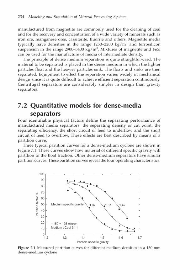
234 Modeling and Simulation of Mineral Processing Systems
100
90
80
70
60
50
40
30
20
10
01.2 1.3 1.4 1.5 1.6 1.7
–150 + 125 micronMedium : Coal 3 : 1
Medium specific gravity 1.32 1.37 1.42
Particle specific gravity
Par
titio
n fa
ctor
%
manufactured from magnetite are commonly used for the cleaning of coaland for the recovery and concentration of a wide variety of minerals such asiron ore, manganese ores, cassiterite, fluorite and others. Magnetite mediatypically have densities in the range 1250–2200 kg/m3 and ferrosiliconsuspension in the range 2900–3400 kg/m3. Mixtures of magnetite and FeSican be used for the manufacture of media of intermediate density.
The principle of dense medium separation is quite straightforward. Thematerial to be separated is placed in the dense medium in which the lighterparticles float and the heavier particles sink. The floats and sinks are thenseparated. Equipment to effect the separation varies widely in mechanicaldesign since it is quite difficult to achieve efficient separation continuously.Centrifugal separators are considerably simpler in design than gravityseparators.
7.2 Quantitative models for dense-mediaseparators
Four identifiable physical factors define the separating performance ofmanufactured media separators: the separating density or cut point, theseparating efficiency, the short circuit of feed to underflow and the shortcircuit of feed to overflow. These effects are best described by means of apartition curve.
Three typical partition curves for a dense-medium cyclone are shown inFigure 7.1. These curves show how material of different specific gravity willpartition to the float fraction. Other dense-medium separators have similarpartition curves. These partition curves reveal the four operating characteristics.
Figure 7.1 Measured partition curves for different medium densities in a 150 mmdense-medium cyclone

Gravity separation 235
7.2.1 The cut pointThe cut point is defined as the density 50 at which the partition function hasthe value 0.5. A particle having the density 50 has equal chance of reportingto the sink fraction as to the float fraction.
The cut point is an operating parameter that can be controlled fairly easilyby variation of the medium density which obviously determines which particlestend to sink in the medium and which tend to float. In a static bath of densemedium the cut point is always equal to the density of the medium. However,in continuously operating equipment this is not always the case and the cutpoint can be greater or less than the medium density depending on whetherthe lighter or heavier fraction must move counter to the prevailing bulk flowof the medium in the equipment. For example in the dense-medium cyclone,the medium together with the material to be separated enters tangentially onthe periphery of the cylindrical section and the bulk of the medium leavesthrough the vortex finder on the axis. There is therefore an overall flow ofmedium from outside inward and the inward velocity of the medium tendsto drag particles with it towards the center. Any heavy particles that leave thecyclone in the underflow must move against this flow and therefore requirea net negative buoyancy to overcome the viscous drag of the medium. Thusany particle that finds an equilibrium orbit in the cyclone must be denserthan the medium. Since the particles on equilibrium orbits define the cutpoint:
50 > m (7.1)
where m is the density of the medium. The difference 50 – m is called thecut point shift and this can be normalized with respect to the medium densityto form the normalized cut point shift:
NCPS = –50 m
m(7.2)
The normalized cut point shift must obviously increase as particle size decreasesand experimental data for coal in a dense-medium cyclone are correlated bythe simple power law:
NCPS = 0.4 –0.32dp (7.3)
over the range 0.015 < dp < 1 mm.When the lighter fraction must move counter to a prevailing flow of medium,
the NCPS must be negative. This is quite uncommon because dense mediumdrum separators are usually designed to provide a medium flow counter tothe prevailing force field to ensure that the medium does not settle undergravity or the centrifugal field. This means that the sink material movesagainst a prevailing flow of medium and the cut point shift is positive. Ingeneral the NCPS can be neglected for dense-medium drum type separatorsfor particles larger than a few millimeters.

236 Modeling and Simulation of Mineral Processing Systems
An additional factor that influences the cut point shift is the settling of thedense-medium suspension particularly in centrifugal separators. This inevitablyleads to a density differential between overflow and underflow media. Thecut point shift increases with increased media density differential. Napier-Munn et al. (1992) have evaluated a number of modeling techniques that maybe appropriate for the description of the underflow density in terms of theoperating variables in the dense-medium cyclone. An empirical model thatappears to correlate the data well for smaller diameter cyclones is
u
mi
u
c
o
c
ERe
DD
DD
+ = 1.872 0.0891
–0.0872 1.919
(7.4)
where
ReD
im i i
a =
v(7.5)
is the Reynolds number at the inlet. The symbols used in this correlationhave the following meaning:
u = underflow density,Du = spigot diameter,Do = vortex finder diameter,Di = inlet diameter,vi = velocity in the cyclone inlet,
a = apparent viscosity of the medium.E is an error term that varies strongly with the cyclone diameter and must beestimated for the cyclone that is used.
The partition curves usually normalize well with respect to the cut pointdensity so that partition curves determined at different medium densitieswill be superimposed when they are plotted using a normalized abscissa /
50. This effect is seen in Figure 7.2 where the experimental data of Figure 7.1are plotted against the reduced or normalized density / 50 and the data fallon a single curve.
7.2.2 Short circuit flowsThe curve shown in Figure 7.2 is called the normalized partition curve and itis represented by the symbol R(x) where x represents the normalized density
/ 50. The general characteristics of normalized partition functions are shownin Figure 7.3 and in practice the low- and high-density asymptotes are not at100% and 0% respectively. A fraction of the feed is assumed to pass directlyto the underflow and another fraction to the overflow directly without passingthrough the separation field of the separator. If is the short circuit fractionto sinks and the short circuit fraction to floats, the actual partition factor Rcan be related to an ideal or corrected partition factor Rc by
R(x) = + (1 – – )Rc(x) (7.6)
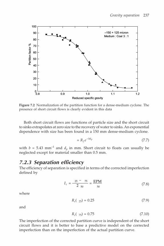
Gravity separation 237
100
90
80
70
60
50
40
30
20
10
0
Par
titio
n fa
ctor
%
0.8 0.9 1.0 1.1 1.2
Reduced specific gravity
–150 + 125 micronMedium : Coal 3 : 1
100
90
80
70
60
50
40
30
20
10
0
Par
titio
n fa
ctor
%
0.8 0.9 1.0 1.1 1.2
Reduced specific gravity
–150 + 125 micronMedium : Coal 3 : 1
Both short circuit flows are functions of particle size and the short circuitto sinks extrapolates at zero size to the recovery of water to sinks. An exponentialdependence with size has been found in a 150 mm dense-medium cyclone.
= –R efbdp (7.7)
with b = 5.43 mm–1 and dp in mm. Short circuit to floats can usually beneglected except for material smaller than 0.5 mm.
7.2.3 Separation efficiencyThe efficiency of separation is specified in terms of the corrected imperfectiondefined by
I c = –
2 = EPM25 75
50 50(7.8)
where
Rc( 25) = 0.25 (7.9)
and
Rc( 75) = 0.75 (7.10)
The imperfection of the corrected partition curve is independent of the shortcircuit flows and it is better to base a predictive model on the correctedimperfection than on the imperfection of the actual partition curve.
Figure 7.2 Normalization of the partition function for a dense-medium cyclone. Thepresence of short circuit flows is clearly evident in this data
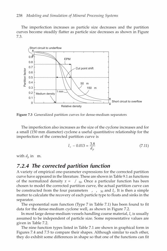
238 Modeling and Simulation of Mineral Processing Systems
Short circuit to underflow
EPM
Short circuit to overflow
0.9
0.8
0.6
0.5
0.4
0.7
0.3
0.2
0.1
0
Cut point shift
50 m
150 m
Relative density
Medium density1 mm
Par
titio
n fa
ctor
The imperfection increases as particle size decreases and the partitioncurves become steadily flatter as particle size decreases as shown in Figure7.3.
Figure 7.3 Generalized partition curves for dense-medium separators
The imperfection also increases as the size of the cyclone increases and fora small (150 mm diameter) cyclone a useful quantitative relationship for theimperfection of the corrected partition curve is
Idc
p– 0.013 = 3.8 (7.11)
with dp in m.
7.2.4 The corrected partition functionA variety of empirical one-parameter expressions for the corrected partitioncurve have appeared in the literature. These are shown in Table 9.1 as functionsof the normalized density x = / 50. Once a particular function has beenchosen to model the corrected partition curve, the actual partition curve canbe constructed from the four parameters , , 50 and Ic. It is then a simplematter to calculate the recovery of each particle type to floats and sinks in theseparator.
The exponential sum function (Type 7 in Table 7.1) has been found to fitdata for the dense-medium cyclone well, as shown in Figure 7.2.
In most large dense-medium vessels handling coarse material, Ic is usuallyassumed to be independent of particle size. Some representative values aregiven in Table 7.2.
The nine function types listed in Table 7.1 are shown in graphical form inFigures 7.4 and 7.5 to compare their shapes. Although similar to each other,they do exhibit some differences in shape so that one of the functions can fit
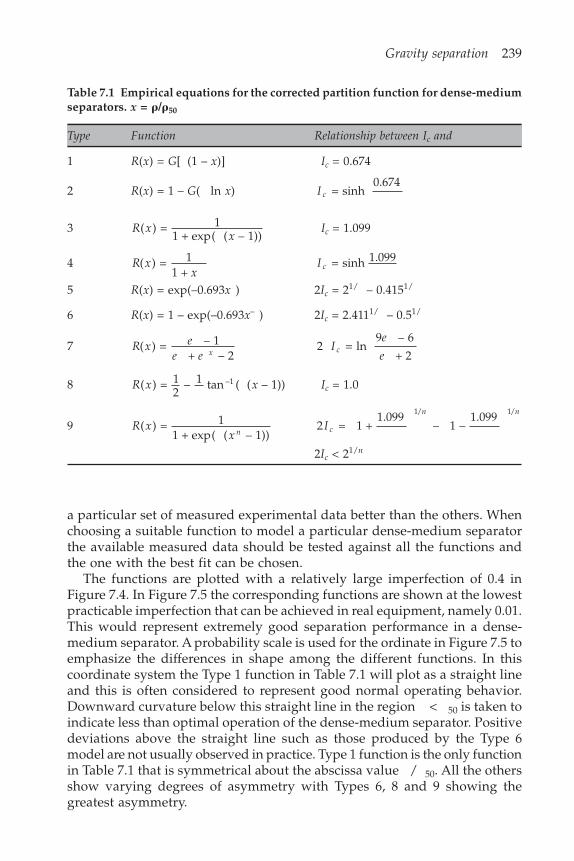
Gravity separation 239
a particular set of measured experimental data better than the others. Whenchoosing a suitable function to model a particular dense-medium separatorthe available measured data should be tested against all the functions andthe one with the best fit can be chosen.
The functions are plotted with a relatively large imperfection of 0.4 inFigure 7.4. In Figure 7.5 the corresponding functions are shown at the lowestpracticable imperfection that can be achieved in real equipment, namely 0.01.This would represent extremely good separation performance in a dense-medium separator. A probability scale is used for the ordinate in Figure 7.5 toemphasize the differences in shape among the different functions. In thiscoordinate system the Type 1 function in Table 7.1 will plot as a straight lineand this is often considered to represent good normal operating behavior.Downward curvature below this straight line in the region < 50 is taken toindicate less than optimal operation of the dense-medium separator. Positivedeviations above the straight line such as those produced by the Type 6model are not usually observed in practice. Type 1 function is the only functionin Table 7.1 that is symmetrical about the abscissa value / 50. All the othersshow varying degrees of asymmetry with Types 6, 8 and 9 showing thegreatest asymmetry.
Table 7.1 Empirical equations for the corrected partition function for dense-mediumseparators. x = �/�50
Type Function Relationship between Ic and
1 R(x) = G[ (1 – x)] Ic = 0.674
2 R(x) = 1 – G( ln x) I c = sinh0.674
3 R xx
( ) = 11 + exp( ( – 1))
Ic = 1.099
4 R xx
( ) = 11 +
I c = sinh 1.099
5 R(x) = exp(–0.693x ) 2Ic = 21/ – 0.4151/
6 R(x) = 1 – exp(–0.693x– ) 2Ic = 2.4111/ – 0.51/
7 R x ee e x
( ) = – 1 + – 2
2 = ln9 – 6
+ 2I
e
ec
8 R x x( ) = 12
– 1 tan ( ( – 1))–1 Ic = 1.0
9 R xx n
( ) = 11 + exp( ( – 1))
2 = 1 + 1.099
– 1 –1.0991/ 1/
I c
n n
2Ic < 21/n

Table 7.2 Typical values of cut point shift and imperfection for dense-medium separators
Separator Cut point Cut point shift Sp. Gr. Imperfection Particle size Referencetype differential
Chance cone 1.54 0.021 Coal1.37 0.01 + 50 mm Leonard (1979)1.37 0.03 12.5 6.5 mm
0.033 0.015
Dense- 1.41 0.020 Coalmedium 1.35 0.018 50 25 mm Leonard (1979)vessel 0.033 12.5 6.3 mm
Dense- 1.49 0.019 1/23/8 Coal
medium 1.50 0.017 3/81/4 Weiss (1985)
cyclone 1.51 0.021 1/4 8#1.53 0.025 8# 14#1.57 0.051 14# 28#
Dense- 1.325 0.045 0.014 1 28# Coalmedium 1.488 0.142 0.015 1 28# Weiss (1985)cyclone
Dense- 3.65 0.59 0.39 0.043 3/16 28# Iron oremedium 3.385 0.54 0.51 0.028 3/16 28# Weiss (1985)cyclone
Dense- 3.065 0.455 0.41 0.036 3/16 65# Chromium oremedium 3.095 0.345 0.27 0.045 3/16 65# Weiss (1985)cyclone 2.907 0.217 0.28 0.018 3/16 35#
3.065 0.215 0.25 0.027 3/16 35#
Dense- 2.82 0.42 0.41 0.028 3/16 28# Magnesitemedium 2.4 0.55 0.58 0.037 3/16 28# Copper orecyclone Davies et al. (1963)

Vorsyl 1.38 0.14 0.025 2 0.5 mm Vanangamudi et al.separator 1.5 0.45 (1992)
Dynawhirl- 1.36 0.050 0.035 31.5 0.75 mm Coalpool 1.52 0.058 0.038 6.3 0.75 mm Leonard (1979)
1.37 0.025 0.018 6.3 0.42 mm
Larcodems 1.658 0.14 0.032 100 0.5 mm Cammack (1987)1.656 0.14 0.038 25 8 mm1.818 0.18 0.176 2 0.5 mm
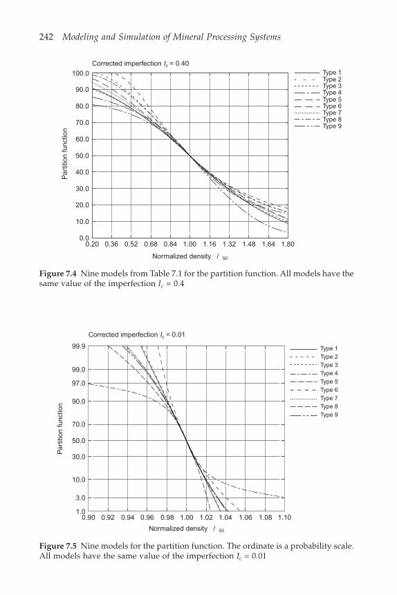
242 Modeling and Simulation of Mineral Processing Systems
Corrected imperfection Ic = 0.01
99.9
99.0
97.0
90.0
70.0
50.0
30.0
10.0
3.0
1.0
Par
titio
n fu
nctio
n
0.90 0.92 0.94 0.96 0.98 1.00 1.02 1.04 1.06 1.08 1.10
Normalized density / 50
Type 1Type 2Type 3Type 4Type 5Type 6Type 7Type 8Type 9
100.0
90.0
80.0
70.0
60.0
50.0
40.0
30.0
20.0
10.0
0.00.20 0.36 0.52 0.68 0.84 1.00 1.16 1.32 1.48 1.64 1.80
Normalized density / 50
Par
titio
n fu
nctio
nType 1Type 2Type 3Type 4Type 5Type 6Type 7Type 8Type 9
Corrected imperfection Ic = 0.40
Figure 7.4 Nine models from Table 7.1 for the partition function. All models have thesame value of the imperfection Ic = 0.4
Figure 7.5 Nine models for the partition function. The ordinate is a probability scale.All models have the same value of the imperfection Ic = 0.01
Gravity separation 243
7.3 Autogenous media separatorsManufactured dense media usually consist of a suspension of heavy particlesthat are sufficiently fine to remain in uniform suspension under the forcefield (gravity or centrifugal) that prevails in the separating unit. The particlesto be separated can move more or less independently of each other and arefree to float or sink depending on their density relative to the apparent densityof the medium suspension. Although particle–particle interactions aresignificant in a manufactured medium separator, they are usually neithersufficiently frequent nor intense to significantly influence the cut point thatis achieved in the separator. However, particle–particle interactions can havea significant influence on the separating efficiency that is actually achieved inthe equipment. In an autogenous medium separator, particle–particleinteractions are significant and dominant since it is the close interactionsbetween the particles that generate the dense environment in which particlescan separate.
The primary phenomenon that occurs in an autogenous medium separatoris stratification in the dense bed of particles. Whenever a bed of particles isdisturbed and is allowed to settle, the particles will exhibit some tendency tostratify. The heavier particles will tend to find their way to the bottom of thebed and the lighter particles will tend to migrate to the top of the bed.Autogenous media separators rely on stratification of the bed to effect aseparation and they are designed to promote rapid and effective stratificationof the particle bed.
The stratification behavior of a particle bed can be described in terms ofthe potential energy of all the particles in the bed. Stratification acts to minimizethe total potential energy of the bed by rearrangement of the particles in thebed. This principle was used by Mayer to provide a quantitative descriptionof the behavior of separation equipment such as the jig. However, aconsideration of potential energy alone does not provide an adequatedescription of the actual stratification process as it occurs in practical operations.No matter how effective the stratifying action of the machine is, perfectstratification is never possible. A multitude of random processes influencethe behavior of each particle during the time that it passes through thestratification zone of the equipment and these combine to destroy the idealstratification pattern that is predicted by potential energy considerations alone.The ideal stratification pattern tends to create sharply defined layers in thebed. Sharp boundaries between layers cannot be maintained in the face of thevariety of random perturbations that are felt by the particles. The sharpboundaries consequently become diffuse by a diffusion type mechanism whichalways acts to oppose the ideal stratification pattern.
Lovell et al. (1994) give a colorful graphic description of the relationshipbetween the pulsation of the jig bed and the motion of the particles as can besensed by inserting the hand into the bed. ‘At the peak of the pulsion stroke,the particles must be free to move relative to each other and during thesuction stroke they should be firmly held by the suction of the bed.’ It is this
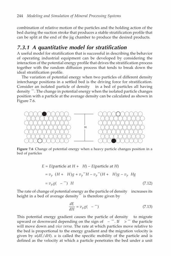
244 Modeling and Simulation of Mineral Processing Systems
H
combination of relative motion of the particles and the holding action of thebed during the suction stroke that produces a stable stratification profile thatcan be split at the end of the jig chamber to produce the desired products.
7.3.1 A quantitative model for stratificationA useful model for stratification that is successful in describing the behaviorof operating industrial equipment can be developed by considering theinteraction of the potential energy profile that drives the stratification processtogether with the random diffusion process that tends to break down theideal stratification profile.
The variation of potential energy when two particles of different densityinterchange positions in a settled bed is the driving force for stratification.Consider an isolated particle of density in a bed of particles all havingdensity . The change in potential energy when the isolated particle changesposition with a particle at the average density can be calculated as shown inFigure 7.6.
Figure 7.6 Change of potential energy when a heavy particle changes position in abed of particles
E = E(particle at H + H) – E(particle at H)
= ( + ) + – ( + ) –v H H g v H v H H g v Hgp p p p
= ( – )v g Hp (7.12)
The rate of change of potential energy as the particle of density increases itsheight in a bed of average density is therefore given by
dEdH
v gp = ( – ) (7.13)
This potential energy gradient causes the particle of density to migrateupward or downward depending on the sign of – . If > the particlewill move down and vice versa. The rate at which particles move relative tothe bed is proportional to the energy gradient and the migration velocity isgiven by u(dE/dH). u is called the specific mobility of the particle and isdefined as the velocity at which a particle penetrates the bed under a unit
Gravity separation 245
potential energy gradient. u is a strong function of particle size and shapeand the bed expansion mechanism but is independent of the particle density.The flux of particles of density in a bed of average density caused by thepotential energy gradient is given by
n C u dEdHs = – m /m s3 2 (7.14)
C is the concentration of particles of density in the bed expressed as thesolid volume fraction. The negative sign reflects the fact that each particlewill tend to move down the potential energy gradient so as to ultimatelyminimize the total potential energy in accordance with Mayer’s principle. nsis called the stratification flux. Combination of Equations 7.13 and 7.14 gives
n C uv gs p = – ( – ) (7.15)
Opposing the stratification flux is the diffusive flux due to the random particle–particle and particle–fluid interactions within the bed. This flux is describedby a Fickian equation of the type
n DdCdHD = – (7.16)
The diffusion coefficient D is dependent on the particle size, shape and bedexpansion mechanism.
A dynamic state of stratification equilibrium exists in the bed when thetendency of the particles to stratify under the influence of the potential energygradient is exactly balanced by tendency to disperse under the influence ofthe concentration gradient that is created by the stratification action. Thisdynamic equilibrium is defined by
nD = –ns (7.17)
so that
dCdH
ugv CD
p = – ( – ) (7.18)
This can be written in terms of the relative height h = ,HHb
where Hb is the
total bed depth and the specific stratification constant
= m /kg3ugv H
Dp b
(7.19)
dCdh
C h = – ( – ( )) (7.20)
is independent of particle density but will be a strong function of particlesize and bed expansion mechanism. The average bed density is a function ofh as indicated in Equation 7.20 and is given by

246 Modeling and Simulation of Mineral Processing Systems
( ) = ( )0
h C h d (7.21)
A solution to Equation 7.20 gives the vertical concentration profile of particlesof density . No boundary conditions can be specified a priori for Equation7.20 because it is not possible to specify the concentration of any particle typeat either the top or bottom or at any intermediate level in the bed.
However, the solution to Equation 7.20 must satisfy the conditions
0
1
= for all C dh C f (7.22)
where C f is the concentration of particles of density in the feed to the bedand
0 = 1 for 0 1C d h (7.23)
In practice the particle population is discretized into n grade classes, each ofwhich has a unique density and Equations 7.20–7.23 are written in discreteform
dC hdh
C h h i nii i
( ) = – ( )( – ( )) for = 1, 2, . . . (7.24)
with
( ) = ( )=1
h C hi
n
i i (7.25)
i
n
iC h h=1
( ) = 1 for all (7.26)
C C h dh iif
i = ( ) for all 0
1
(7.27)
7.3.2 Stratification of a two-component systemThe set of differential Equations 7.24 can be solved easily in closed formwhen the bed consists of only two components.
Formal integral of Equation 7.24 gives
C h C h y dy ii i i
h
( ) = (0) exp – + ( ) for = 1 and 20
(7.28)
The average density of particles at level h in the bed for the two-componentsystem is
Gravity separation 247
= ( ) + ( )( ) + )
1 1 2 2
1 2
C h C hC h C h(
(7.29)
The boundary condition Ci(0) represents the concentration of particles oftype i at the base of the bed. This is an unknown and must be calculated foreach species but the solution must satisfy the two conditions 7.26 and 7.27.
Equation 7.26 requires
C1(0) + C2(0) = 1 (7.30)
at every level in the bed.The vertical density profile ( )h is also unknown so that Equation 7.28
cannot be used in isolation to calculate the vertical concentration profile ofthe different particle types. However, the ratio of the concentrations of thetwo species in a two-component system is independent of ( ).h
C hC h
C hC h
CC
h1
2
1
1
1
21 2
)) =
( )1 – ( )
= (0)(0)
exp [– ( – ) ]((
(7.31)
from which
C h
CC
h
CC
h1
1
21 2
1
21 2
( ) =
(0) exp[– ( – ) ]
1 + (0)(0)
exp[– ( – ) ]
( )0(7.32)
Equation 7.32 gives the vertical concentration profile of species 1 as a functionof the ratio C1(0)/C2(0) at the bottom of the bed. This ratio is fixed by thecomposition of the material that is fed to the jig bed and can be evaluatedfrom Equation 7.27.
C C h dhf1
0
1
1 = )( (7.33)
Integration of Equation 7.33 using Equation 7.32 and solution for C C1 2(0)/ (0)gives:
CC
C
C
f
f1
2
1 2 1
2 1 2
1 2(0)(0)
= 1 – exp [– ( – ) ]
exp[– ( – ) ] –1 exp[ ( – )] (7.34)
which is easy to evaluate when the composition of the feed is known.Substitution of this ratio into Equation 7.32 gives the vertical concentrationprofile. Typical concentration profiles are shown in Figure 7.7.
The grade and recovery in the two product streams can be calculated oncethe equilibrium stratification profiles have been calculated. The yield of totalsolids to the heavier fraction can be obtained by integrating the concentrationprofile.
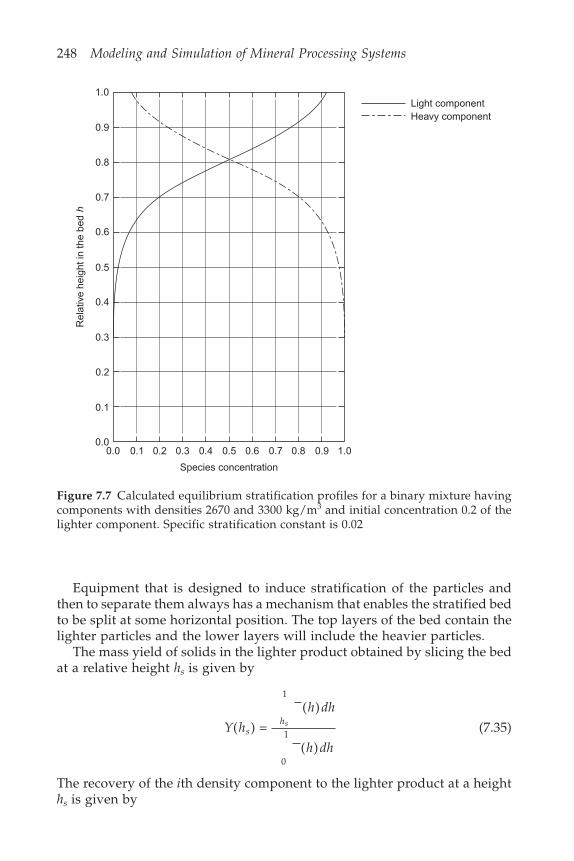
248 Modeling and Simulation of Mineral Processing Systems
1.0
0.9
0.8
0.7
0.6
0.5
0.4
0.3
0.2
0.1
0.0
Rel
ativ
e he
ight
in th
e be
d h
Species concentration
0.0 0.1 0.2 0.3 0.4 0.5 0.6 0.7 0.8 0.9 1.0
Light componentHeavy component
Equipment that is designed to induce stratification of the particles andthen to separate them always has a mechanism that enables the stratified bedto be split at some horizontal position. The top layers of the bed contain thelighter particles and the lower layers will include the heavier particles.
The mass yield of solids in the lighter product obtained by slicing the bedat a relative height hs is given by
Y h
h dh
h dhs
hs( ) =
( )
( )
1
0
1 (7.35)
The recovery of the ith density component to the lighter product at a heighths is given by
Figure 7.7 Calculated equilibrium stratification profiles for a binary mixture havingcomponents with densities 2670 and 3300 kg/m3 and initial concentration 0.2 of thelighter component. Specific stratification constant is 0.02
Gravity separation 249
R h
C h dh
C h dh
C h dh
Ci s
hi
i
hi
if
s s( ) =
( )
( )
=
( )1
0
1
1
(7.36)
The concentration of component i in the lighter product is given by
CC R h
C R hiP i
fi s
i if
i s
= ( )
( )(7.37)
Equations 7.35, 7.36 and 7.37 can be used to generate grade–recovery andrecovery–yield curves using the relative splitting height hs as the operatingvariable.
7.3.3 Stratification in multicomponent bedsWhen the material to be processed contains more than two particle types, theconvenient analytical solution given in the previous section is no longeravailable and a numerical technique must be used to solve the system ofdifferential Equations 7.24 subject to the conditions 7.25 to 7.27.
One obvious approach to the solution of the system of Equations 7.24 is toassume a set of Ci(0), integrate Equations 7.24 numerically and check theresulting profiles against Equation 7.27. Using an optimization procedure,the initial guesses of Ci(0) can be refined and the procedure repeated. Thisprocedure, however, converges only slowly and exhibits weak stabilitycharacteristics.
A much more efficient procedure for integrating the equilibrium equationscan be developed using the following method.
Integration of the stratification Equations 7.24 from the bottom of the bedwith the unknown initial condition C Ci i(0) = 0 gives
C h C h u du i ni i i
h
( ) = exp – + ( ) = 1, 2, 3 . . . 0
0(7.38)
Substituting Equation 7.38 into Equation 7.27
0
10
0 exp – + ( ) = C h u du dh Ci i
h
if (7.39)
and rearranging gives an estimate of the concentration of each species at thebottom of the bed
CC
h u du dhi
if
i
h0
0
1
0
=
exp – + ( )
(7.40)
250 Modeling and Simulation of Mineral Processing Systems
An iterative method is started by guessing an initial average density profile( )h and applying Equation 7.40 to calculate Ci
0 for each particle type.Accumulation of numerical errors i prevented by normalizing the Ci(0) to
make
i iC (0) = 1 (7.41)
at this stage in the calculation.These initial values Ci(0) can be used in Equation 7.38 to get an estimate of
the concentration profiles Ci(h) for each particle type and then a new averagedensity profile can be calculated using Equation 7.25. The procedure is repeatedand continued until the calculated average density profile no longer changesfrom one iteration to the next.
This iterative procedure is efficient and robust and is capable of generatingsolutions rapidly for any number of components encountered in practice.The ideal Meyer profile has been found to provide a good starting point andthis is easy to calculate.
The solution for a hypothetical four-component mixture is illustrated inFigure 7.9, which shows a typical equilibrium stratification profile and comparesit to the ideal Mayer profile that would be achieved without dispersion.
Specific stratification constant values range from zero for a perfectly mixedbed with no stratification to infinity for perfect stratification. Typical practicalvalues of alpha range from 0.001 m3/kg for a poor separation to 0.5 m3/kgfor an exceedingly accurate separation. Although independent of thewashability distribution of the feed, the specific stratification constant isdependent on the size and shape of the particles and on the type of equipmentand its operating conditions. Experience has shown that this method is rapidlyconvergent over a wide range of conditions. As an example the calculatedconcentration profiles of nine washability fractions of coal in an industrialBaum jig are shown in Figure 7.8.
7.3.4 Performance of continuously operating single-and double-stage jigs
The mineral jig is designed specifically to stratify a bed of solid particles anda number of different designs have evolved over the years. These all have acommon basic operating principle so that it is feasible to build a genericmodel that can be used to simulate the operation of any continuous jig.
Three distinct subprocesses can be identified in a continuous jig: bedstratification produced by the vertical pulsation of the bed, longitudinaltransport of the bed due to water flow along the axis of the jig and splittingof the bed into concentrate and tailing layers.
The water velocity in the longitudinal direction is not uniform and verticalvelocity profile exists in the continuous jig. In each compartment of the jigthe various bed layers move at different velocities, with the upper layersgenerally moving faster than the lower ones. The velocities of particles at the

Gravity separation 251
1.0
0.8
0.6
0.4
0.2
0.00.0 0.2 0.4 0.6 0.8 1.0
Con
cent
ratio
n-m
ass
frac
tion
Relative densityfraction
1.36
1.451.575
1.75
1.925
2.1
2.32.6
3.1
Relative height in stratified bed
Estimatedcut height
Figure 7.8 Calculated stratification profiles for nine washability fractions of coal inan industrial jig (Tavares and King, 1995)
Figure 7.9 The effect of dispersion on the equilibrium stratification profile in amulticomponent mixture. The beds shown represent accurate simulations using theideal Mayer theory and the dispersion model. The calculated vertical concentrationprofiles are also shown. A value of = 0.03 was used to simulate the dispersed bed
Density = 1.35 Density = 1.5 Density = 1.7 Density = 2.1
Ideal equilibrium stratificationas predicted by Mayer’s theory
Volumeconcentration
Actual equilibrium stratification aspredicted by the dispersion model
Volumeconcentration
1.0
0.5
0.0 0.
00.
250.
50.
751.
0
Rel
ativ
e he
ight
in b
ed
1.0
0.5
0.0 0.
00.
250.
50.
751.
0
Rel
ativ
e he
ight
in b
ed
252 Modeling and Simulation of Mineral Processing Systems
end of the bed depend primarily on the velocities of the layers to which theyreport. The velocity profile at the discharge end of the bed determines thedischarge rate of each layer as it leaves the jig. In a continuous jig the overallmaterial balance must be satisfied for each component and the integral conditionEquation 7.27 must reflect the velocity profile and is replaced by
CC h V h dh
C h V h dhd
f = ( ) ( )
) ( )
0
1
0 0
1
(
(7.42)
where V(h) is the longitudinal velocity of the bed at height h.The velocity profile must be known in order to integrate Equation 7.42.
The actual longitudinal velocity at each bed height can only be determinedby experiment for any particular equipment type and it will depend on theoperating conditions in the unit. Defining a dimensionless velocity by v(h) =(V(h)/Vmax) and discretizing Equation 7.42 we get
CC h v h dh
C h v h dhif
i
j
n
j
= ( ) ( )
( ) ( )
0
1
=1 0
1(7.43)
The continuous jigging model for monosize feeds consists of Equations7.24 subjected to the integral conditions given in Equations 7.25 and 7.43. Letthe denominator of Equation 7.43 be equal to a constant, say 1/ , then
C C h v h dhif
i = ( ) ( )0
1
(7.44)
A similar iterative solution procedure to the one described in Section 7.3.2 isused to model equipment with a significant velocity profile. SubstitutingEquation 7.44 into Equation 7.38 and rearranging,
CC
h u du v h dhio i
f
i
h =
exp – + ( ) ( )0
1
0
(7.45)
Cio is determined iteratively as before and Ci
o is obtained from
CC
Cio i
o
j
n
jo
=
=1
(7.46)
In the jigging process, particularly for well-operated jigs, the longitudinalvelocity is expected to increase monotonically from the bottom to the top of
Gravity separation 253
the bed. The limited amount of direct measurements of velocity profiles foundin the literature, however, does not allow the development of precise modelsfor the velocity profile. A simple but effective empirical model for the velocityprofile, which does not appear to conflict with the available experimentaldata is used here and is given by
v(h) = h + (1 – )h2 (7.47)
where is a parameter of the model.In a continuous jig, the separation of stratified layers is affected by refuse
and middlings discharge mechanisms. Additional misplacement of clean coaland refuse is believed to happen as a result of the turbulence produced by theoperation of these removal systems. The absence of any quantitativeexperimental work on this effect and the wide variety of refuse ejectorsencountered in practice does not allow the precise modeling of this sub-process at present. A simple model which considers that the turbulenceproduced by splitting the stratified layers creates a perfectly mixed region ofrelative thickness 2 is proposed tentatively here. The yield of solids to thelighter product can now be calculated by
Y h
h v h dh h v h dh
h v h dhs
h
h
hs
s
s( , ) =
12
( ) ( ) + ( ) ( )
( ) ( )
–
+
+
1
0
1 (7.48)
The recovery of the ith density component to the lighter product is given by
R h
C h v h dh C h v h dh
C h v h dhi s
h
h
ih
i
i
s
s
s( , ) =
12
( ) ( ) + ( ) ( )
( ) ( )
–
+
+
1
0
1 (7.49)
The density distribution of the lighter product by volume is given by
C hC R h
C R hip
sif
i s
j
n
jf
j s
( , ) = ( , )
( , )=1
(7.50)
The effect of the velocity profile can be seen by comparing the simulated bedsin Figures 7.9 and 7.10. In each case the same hypothetical four-componentmixture was used to simulate the stratified beds. A thick layer of refuseaccumulates in the bottom of the moving bed as a result of the longer residencetimes experienced by the heavier material in the jig. The concentration of theseparate components in the lighter product stream is governed by Equation7.50 and differs significantly from the equilibrium concentration in the beditself.
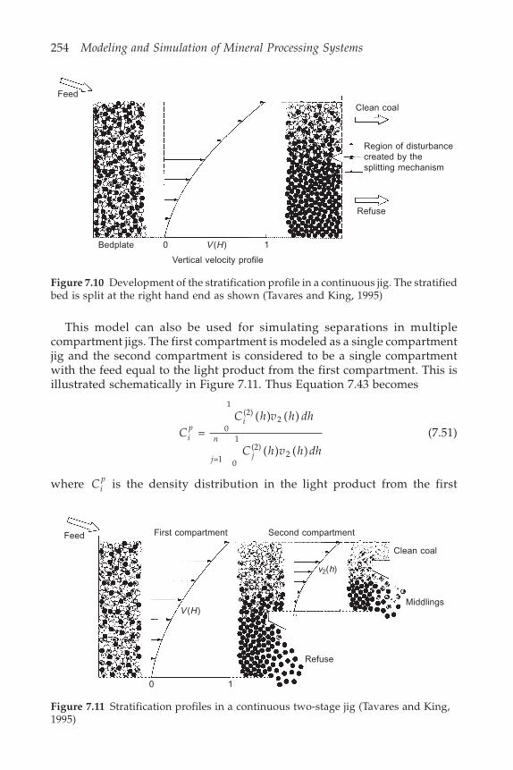
254 Modeling and Simulation of Mineral Processing Systems
This model can also be used for simulating separations in multiplecompartment jigs. The first compartment is modeled as a single compartmentjig and the second compartment is considered to be a single compartmentwith the feed equal to the light product from the first compartment. This isillustrated schematically in Figure 7.11. Thus Equation 7.43 becomes
CC h v h dh
C h v h dhip
i
j
n
j
= ) )
( ) ( )
0
1(2)
2
=1 0
1(2)
2
( ((7.51)
where Cip is the density distribution in the light product from the first
Feed
Bedplate 0 V(H) 1
Refuse
Region of disturbancecreated by thesplitting mechanism
Vertical velocity profile
Clean coal
Figure 7.10 Development of the stratification profile in a continuous jig. The stratifiedbed is split at the right hand end as shown (Tavares and King, 1995)
Feed First compartment Second compartment
V (H)
0 1
Refuse
v2(h)
Clean coal
Middlings
Figure 7.11 Stratification profiles in a continuous two-stage jig (Tavares and King,1995)
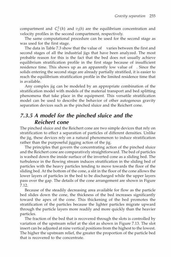
Gravity separation 255
compartment and C hi2 ( ) and v2(h) are the equilibrium concentration and
velocity profiles in the second compartment, respectively.The same computational procedure can be used for the second stage as
was used for the first stage.The data in Table 7.3 show that the value of varies between the first and
second stages of all the industrial jigs that have been analyzed. The mostprobable reason for this is the fact that the bed does not usually achieveequilibrium stratification profile in the first stage because of insufficientresidence time. This shows up as an apparently low value of . Since thesolids entering the second stage are already partially stratified, it is easier toreach the equilibrium stratification profile in the limited residence time thatis available.
Any complex jig can be modeled by an appropriate combination of thestratification model with models of the material transport and bed splittingphenomena that take place in the equipment. This versatile stratificationmodel can be used to describe the behavior of other autogenous gravityseparation devices such as the pinched sluice and the Reichert cone.
7.3.5 A model for the pinched sluice and theReichert cone
The pinched sluice and the Reichert cone are two simple devices that rely onstratification to effect a separation of particles of different densities. Unlikethe jig, these devices rely on a natural phenomenon to induce stratificationrather than the purposeful jigging action of the jig.
The principles that govern the concentrating action of the pinched sluiceand the Reichert cone are comparatively straightforward. The bed of particlesis washed down the inside surface of the inverted cone as a sliding bed. Theturbulence in the flowing stream induces stratification in the sliding bed ofparticles with the heavy particles tending to move towards the floor of thesliding bed. At the bottom of the cone, a slit in the floor of the cone allows thelower layers of particles in the bed to be discharged while the upper layerspass over the gap. The details of the cone arrangement are shown in Figure7.12.
Because of the steadily decreasing area available for flow as the particlebed slides down the cone, the thickness of the bed increases significantlytoward the apex of the cone. This thickening of the bed promotes thestratification of the particles because the lighter particles migrate upwardthrough the particle layers more readily and more quickly than the heavierparticles.
The fraction of the bed that is recovered through the slots is controlled byvariation of the upstream relief at the slot as shown in Figure 7.13. The slotinsert can be adjusted at nine vertical positions from the highest to the lowest.The higher the upstream relief, the greater the proportion of the particle bedthat is recovered to the concentrate.

Table 7.3 Application of the multicomponent continuous model to the operation of industrial jigs
Size Measured Estimated Calculated cut Calculated bedJig (mm) Stage yield value of height density at the
(%) hs cutter position( )hs
Baum 1 150 1.4 Primary 30.6 0.027 0.56 1.78Secondary 13.1 0.091 0.39 1.56
Baum 2 100 1.4 Primary 44.5 0.046 0.65 1.45Baum 3 50 1 Primary 20.6 0.009 0.49 2.10
Secondary 30.1 0.028 0.56 1.95Baum 4 50 0.6 Primary 5.0 0.006 0.27 2.56
Secondary 71.7 0.114 0.83 1.77Batac 1 12 0.6 Primary 7.4 0.019 0.30 3.40
Secondary 96.4 0.113 0.98 1.68Batac 2 19 0.6 Primary 14.8 0.028 0.39 2.23
Secondary 17.3 0.072 0.42 1.66Batac 3 50 0.6 Primary 15.2 0.068 0.42 1.70

Gravity separation 257
Feed
No concentration at this end
Bed depth increases as the bedslides down the cone
Lighter materialcrosses the gap
Stratification develops as bedslides down cone
Stratified bed is split at the gap
Heavier particles fall throughthe gap
Two well-documented experimental studies on the behavior of the Reichertprovide some excellent data from which the essential nature of the operationof the Reichert cone can be established and a useful predictive model can bedeveloped. Forssberg and Sandstrain (1979) and Holland-Batt (1978).
Schematics of the four standard Reichert cone modules are shown in Figures7.14 and 7.15. A basic cone module can consist of a single separating cone orthe flow can be split on to two cone surfaces, as shown in Figures 7.14 and7.15 which allows the cone to handle a greater feed. Two multiple cone modulesare common: the DSV module which consists of a double cone followed by asingle cone with a variable gap, and the DSVSV module which has an extrasingle cone with variable gap to clean the concentrate further. The two cleaningstages of the DSVSV module makes this configuration more suitable for cleaning
Figure 7.12 Details of the concentrating action of the Reichert cone. A double coneis illustrated
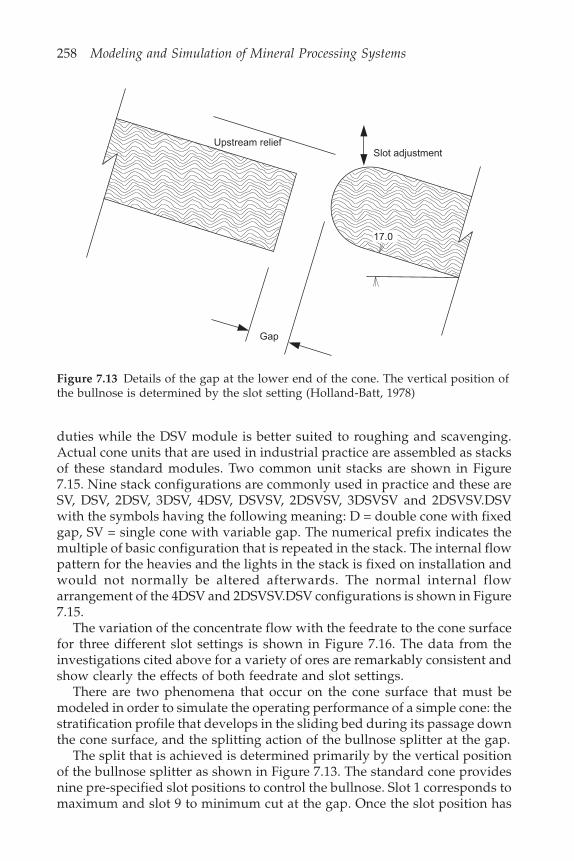
258 Modeling and Simulation of Mineral Processing Systems
Upstream reliefSlot adjustment
Gap
17.0
duties while the DSV module is better suited to roughing and scavenging.Actual cone units that are used in industrial practice are assembled as stacksof these standard modules. Two common unit stacks are shown in Figure7.15. Nine stack configurations are commonly used in practice and these areSV, DSV, 2DSV, 3DSV, 4DSV, DSVSV, 2DSVSV, 3DSVSV and 2DSVSV.DSVwith the symbols having the following meaning: D = double cone with fixedgap, SV = single cone with variable gap. The numerical prefix indicates themultiple of basic configuration that is repeated in the stack. The internal flowpattern for the heavies and the lights in the stack is fixed on installation andwould not normally be altered afterwards. The normal internal flowarrangement of the 4DSV and 2DSVSV.DSV configurations is shown in Figure7.15.
The variation of the concentrate flow with the feedrate to the cone surfacefor three different slot settings is shown in Figure 7.16. The data from theinvestigations cited above for a variety of ores are remarkably consistent andshow clearly the effects of both feedrate and slot settings.
There are two phenomena that occur on the cone surface that must bemodeled in order to simulate the operating performance of a simple cone: thestratification profile that develops in the sliding bed during its passage downthe cone surface, and the splitting action of the bullnose splitter at the gap.
The split that is achieved is determined primarily by the vertical positionof the bullnose splitter as shown in Figure 7.13. The standard cone providesnine pre-specified slot positions to control the bullnose. Slot 1 corresponds tomaximum and slot 9 to minimum cut at the gap. Once the slot position has
Figure 7.13 Details of the gap at the lower end of the cone. The vertical position ofthe bullnose is determined by the slot setting (Holland-Batt, 1978)
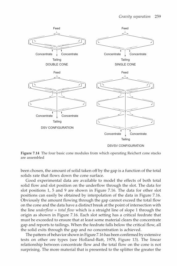
Gravity separation 259
Feed
Concentrate Concentrate
Tailing
DOUBLE CONE
Feed
Concentrate Concentrate
Tailing
DSV CONFIGURATION
Feed
Concentrate Concentrate
Tailing
SINGLE CONE
Feed
Concentrate Concentrate
Tailing
DSVSV CONFIGURATION
been chosen, the amount of solid taken off by the gap is a function of the totalsolids rate that flows down the cone surface.
Good experimental data are available to model the effects of both totalsolid flow and slot position on the underflow through the slot. The data forslot positions 1, 5 and 9 are shown in Figure 7.16. The data for other slotpositions can easily be obtained by interpolation of the data in Figure 7.16.Obviously the amount flowing through the gap cannot exceed the total flowon the cone and the data have a distinct break at the point of intersection withthe line underflow = total flow which is a straight line of slope 1 through theorigin as shown in Figure 7.16. Each slot setting has a critical feedrate thatmust be exceeded to ensure that at least some material clears the concentrategap and reports to tailings. When the feedrate falls below the critical flow, allthe solid exits through the gap and no concentration is achieved.
The pattern of behavior shown in Figure 7.16 has been confirmed by extensivetests on other ore types (see Holland-Batt, 1978, Figure 13). The linearrelationship between concentrate flow and the total flow on the cone is notsurprising. The more material that is presented to the splitter the greater the
Figure 7.14 The four basic cone modules from which operating Reichert cone stacksare assembled

260 Modeling and Simulation of Mineral Processing Systems
FeedFeed
Concentrate
Concentrateor middling
Concentrateor middling
Tailing
2DSVSV.DSV stack Concentrateor middling
Tailing
4DSV stack
Concentrateor middling
Concentrateor middling
Concentrate
flow through the gap. The point of convergence, POC in Figure 7.16, and theslopes of the lines vary with ore type and Table 7.4 summarizes the data thatare available. These variations are probably associated primarily with theshape of the particles but this effect has never been investigated.
In order to calculate the composition of the two discharge streams fromthe cone, it is necessary to model the stratification of the solid particles thatoccurs during the passage of the sliding bed down the cone surface. Stratificationis a complex process, but a good realistic quantitative description of thisphenomenon on the cone is provided by the equilibrium profile that balancesthe potential energy decrease that occurs with stratification against the random
Figure 7.15 2DSVSV.DSV and 4DSV Reichert cone stacks that are commonly used forcleaning and roughing duties respectively
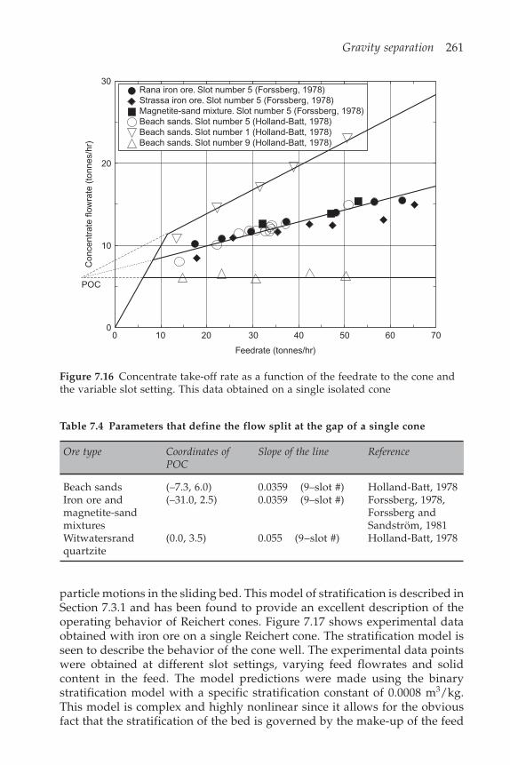
Gravity separation 261
Rana iron ore. Slot number 5 (Forssberg, 1978)Strassa iron ore. Slot number 5 (Forssberg, 1978)Magnetite-sand mixture. Slot number 5 (Forssberg, 1978)Beach sands. Slot number 5 (Holland-Batt, 1978)Beach sands. Slot number 1 (Holland-Batt, 1978)Beach sands. Slot number 9 (Holland-Batt, 1978)
30
20
10
POC
00 10 20 30 40 50 60 70
Feedrate (tonnes/hr)
Con
cent
rate
flow
rate
(to
nnes
/hr)
particle motions in the sliding bed. This model of stratification is described inSection 7.3.1 and has been found to provide an excellent description of theoperating behavior of Reichert cones. Figure 7.17 shows experimental dataobtained with iron ore on a single Reichert cone. The stratification model isseen to describe the behavior of the cone well. The experimental data pointswere obtained at different slot settings, varying feed flowrates and solidcontent in the feed. The model predictions were made using the binarystratification model with a specific stratification constant of 0.0008 m3/kg.This model is complex and highly nonlinear since it allows for the obviousfact that the stratification of the bed is governed by the make-up of the feed
Figure 7.16 Concentrate take-off rate as a function of the feedrate to the cone andthe variable slot setting. This data obtained on a single isolated cone
Table 7.4 Parameters that define the flow split at the gap of a single cone
Ore type Coordinates of Slope of the line ReferencePOC
Beach sands (–7.3, 6.0) 0.0359 (9–slot #) Holland-Batt, 1978Iron ore and (–31.0, 2.5) 0.0359 (9–slot #) Forssberg, 1978,magnetite-sand Forssberg andmixtures Sandström, 1981Witwatersrand (0.0, 3.5) 0.055 (9–slot #) Holland-Batt, 1978quartzite

262 Modeling and Simulation of Mineral Processing Systems
material. The model is computationally intensive since it requires the solutionof a set of coupled differential equations – one for each type of particle – withintegral boundary conditions. Once the behavior of a single cone can bemodeled, the behavior of an entire cone stack can be synthesized by combiningthe models for the single cones appropriately. The double cone is synthesizedas two single cones in parallel, each one receiving one half of the feed to thestage.
The calculation of the performance of a single module and a compositecone stack proceeds as follows:
1. Calculate the composition (distribution of particle size and particlecomposition) of the feed to the stage. This may be the gap underflowfrom the previous stage or it may be the combined concentrates and/or rejects from several stages higher up in the cone stack or from otherunits in the plant or it may be the plant feed itself.
2. Use the stratification model to calculate the equilibrium stratificationprofile of the sliding bed at the gap using the feed from step 1 as themodel input.
3. Calculate the gap take-off flowrate from the flow model described byFigure 7.16 and Table 7.4.
4. Split the calculated stratified bed at the horizontal level that will givethe correct gap take-off established in step 3.
5. Integrate the stratified bed from the floor to the splitting level andfrom the splitting level to the top of the bed to calculate the compositionof the concentrate and discard streams.
6. Use these streams to constitute the feeds to the lower cones on thestack and repeat steps 1–5 as necessary.
7. Combine all the concentrates and discards from the cone stackappropriately to constitute the concentrate, middlings, and tailingsfrom the unit.
The composition of the concentrate stream is established by the stratificationthat occurs while the bed of solids is sliding down the inside surface of theseparating cone. Provided that the residence time on the cone is sufficientlylong to allow the equilibrium stratification pattern to be established, thecomposition of the concentrate stream can be calculated using the equilibriumstratification profile as described in Sections 7.3.2 and 7.3.3.
It is comparatively straightforward to apply the model developed aboveto each stage in a stack and then to combine the concentrate streamsappropriately to model the entire cone unit. This is the approach taken inMODSIM, which allows any of the standard configurations of the cone to besimulated.
Although each individual cone in the stack produces only a concentrateand tailings stream, the cone stack as a whole can be configured to producea concentrate, a tailing, and, if required, a middling. A middling stream canbe constituted from the concentrate streams produced by the lower cones in
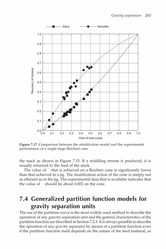
Gravity separation 263
Silica Hematite
1.0
0.9
0.8
0.7
0.6
0.5
0.4
0.3
0.2
0.1
0.00.0 0.1 0.2 0.3 0.4 0.5 0.6 0.7 0.8 0.9 1.0
Rec
over
y of
min
eral
Yield of total solids
the stack as shown in Figure 7.15. If a middling stream is produced, it isusually returned to the feed of the stack.
The value of that is achieved on a Reichert cone is significantly lowerthan that achieved in a jig. The stratification action of the cone is simply notas efficient as in the jig. The experimental data that is available indicates thatthe value of should be about 0.002 on the cone.
7.4 Generalized partition function models forgravity separation units
The use of the partition curve is the most widely used method to describe theoperation of any gravity separation unit and the general characteristics of thepartition function are described in Section 7.2.3. It is always possible to describethe operation of any gravity separator by means of a partition function evenif the partition function itself depends on the nature of the feed material, as
Figure 7.17 Comparison between the stratification model and the experimentalperformance of a single-stage Reichert cone
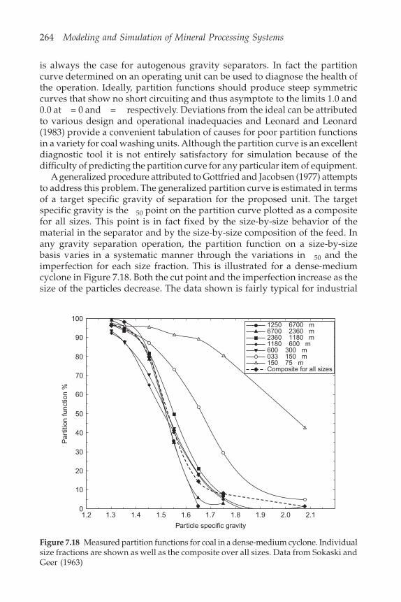
264 Modeling and Simulation of Mineral Processing Systems
1250 6700 m
2360 1180 m1180 600 m600 300 m033 150 m150 75 mComposite for all sizes
6700 2360 m
100
90
80
70
60
50
40
30
20
10
01.2 1.3 1.4 1.5 1.6 1.7 1.8 1.9 2.0 2.1
Particle specific gravity
Par
titio
n fu
nctio
n %
is always the case for autogenous gravity separators. In fact the partitioncurve determined on an operating unit can be used to diagnose the health ofthe operation. Ideally, partition functions should produce steep symmetriccurves that show no short circuiting and thus asymptote to the limits 1.0 and0.0 at = 0 and = respectively. Deviations from the ideal can be attributedto various design and operational inadequacies and Leonard and Leonard(1983) provide a convenient tabulation of causes for poor partition functionsin a variety for coal washing units. Although the partition curve is an excellentdiagnostic tool it is not entirely satisfactory for simulation because of thedifficulty of predicting the partition curve for any particular item of equipment.
A generalized procedure attributed to Gottfried and Jacobsen (1977) attemptsto address this problem. The generalized partition curve is estimated in termsof a target specific gravity of separation for the proposed unit. The targetspecific gravity is the 50 point on the partition curve plotted as a compositefor all sizes. This point is in fact fixed by the size-by-size behavior of thematerial in the separator and by the size-by-size composition of the feed. Inany gravity separation operation, the partition function on a size-by-sizebasis varies in a systematic manner through the variations in 50 and theimperfection for each size fraction. This is illustrated for a dense-mediumcyclone in Figure 7.18. Both the cut point and the imperfection increase as thesize of the particles decrease. The data shown is fairly typical for industrial
Figure 7.18 Measured partition functions for coal in a dense-medium cyclone. Individualsize fractions are shown as well as the composite over all sizes. Data from Sokaski andGeer (1963)
Gravity separation 265
gravity separators and the cut point for the individual sizes is modeled by
rSGSG
fd
ds
s
p
p = = (7.52)
where SGs is the cut point for particles of size dp, SGs is the overall cut point
for the composite feed and dp is the average particle size in the feed. Thisnormalization of the Gottfried-Jacobsen procedure with respect to averageparticle size in the feed is quite robust and correlates much of the data availablein the literature and the function f( ) is not very sensitive to the feed compositionand allows, at least approximately, for fairly wide variations in the sizedistribution in the feed. SGs in Equation 7.52 is the target cut point and thistarget fixes the operating point of the particular unit. The function f( ) hasbeen evaluated for a number of gravity separation units and the followingexponential form fits the data reasonably well
r a b cd
dpi
p = + exp – (7.53)
Values of a, b and c for some different units are given in Table 7.5.
Table 7.5 Parameters to relate cut points for narrow size fractions to the compositecut point
Unit type a b c
Water-only cyclone 0.8 0.6 1.26Dense-medium cyclone 0.98 0.1 1.61Shaking table 0.97 0.3 7.7Coal washing drum 0.98 0.1 1.61
Once the target specific gravity and the average particle size in the feedare known, the cut point for each size of particle can be obtained from Equation7.53. The cut point can be used with any appropriate generalized partitionfunction such as those given in Table 7.1. An appropriate amount of shortcircuiting to either floats or sinks can also be applied if it is anticipated thatthis kind of inefficiency will be present in the equipment.
Osborne (1988) recommends that the variation of EPM with particle size,equipment size and separation density should be computed using a series offactors
EPM = f1 f2 f3Es (7.54)
f1 is a factor accounting for the variation of EPM with particle size, f2 a factoraccounting for variation of EPM with equipment size and f3 a manufacturer’s
266 Modeling and Simulation of Mineral Processing Systems
guarantee factor usually in the range 1.1 to 1.2. Es is a standard functionrepresenting the variation of EPM with separation density for each type ofequipment. Es for various types of coal washing equipment are:
Dense-medium cyclone: Es = 0.027 50 – 0.01Dynawhirlpool: Es = 0.15 50 – 0.16Dense-medium bath: Es = 0.047 50 – 0.05Baum jig: Es = 0.78( 50( 50 – 1) + 0.01)Water-only cyclone: Es = 0.33 50 – 0.31Shaking table and spiral concentrator: Es = 50 – 1
For dense-medium cyclones f1 varies from 2 to 0.75 as particle size variesfrom 0.5 mm to 10 mm.
For dense-medium vessels f1 varies from 0.5 for coarse coal to 1.4 for smallcoal.
Because both the Baum jig and the water-only cyclone are autogenousgravity separators, f1 is dependent on the size distribution and washability ofthe feed material. Values of f1 for jigs range from 3 to 0.5 as the average sizeof the feed material varies from 1 mm to 100 mm.
BibliographyThe model for the Reichert cone is based on data presented by Holland-Batt(1978) and Forssberg and Sandström (1979; 1981).
ReferencesCammack, P. (1987) The LARCODEMS – a new dense medium separator for 100 mm–
0.5 mm raw coal. Aufbereitungs-Technik, Vol. 28, pp. 427–434.Davies, D.S., Dreissen, H.H. and Oliver, R.H. (1965) Advances in hydrocylone heavy
media separation technology for fine ores. Proc. 6th Intl Mineral Processing Congress(A. Roberts, ed.), Pergamon Press, pp. 303–321.
Forssberg, E. (1978) Data from Reichert Cone tests. Private communication to author.Forssberg, E. and Sandström, E. (1979) Utilization of the Reichert cone concentrator in
ore processing. Industrie Mineral-Mineralurgie, pp. 223–243.Forssberg, E. and Sandström, E. (1981) Operational characteristics of the Reichert
cone in ore processing. Proc. 13th International Mineral Processing Congress (J. Laskowski,ed.), Warsaw 1979. Elsevier Scientific Publishing Co. Vol. II, pp. 1424–1481.
Gottfried, B.S. and Jacobsen, P.S. (1977) Generalized distribution curve for characterizingthe performance of coal-cleaning equipment. USBM, Washington, RI8238.
Holland-Batt, A.B. (1978) Design of gravity concentration circuits by use of empiricalmathematical models. Proc. 11th Commonwealth Mining and Metallurgical Congress,Institution of Mining and Metallurgy.
Leonard, J.W. (ed.) (1979) Coal Preparation, 4th edition. SME, Lyttleton, CO.Leonard, I.V. and Leonard, J.W. (1983) Using Tromp Curves to Diagnose Performance
Problems in Coal Cleaning. In Basic Mathematics and Computer Techniques for CoalPreparation and Mining (K.K. Humphreys and J.W. Leonard, eds), Marcel DekkerInc., pp. 71–79.
Gravity separation 267
Lovell, H.L., Moorehead, R.G., Luckie, P.T. and Kindig, J.K. (1994) Hydraulic Separation.Chapter 7 in Coal Preparation (J.W. Leonard, ed.), 5th edition, SME, Lyttleton, CO,p. 307.
Napier-Munn, T.J., Scott, I.A., Tuteja, R., Davis, J.J. and Kojovic, T. (1992) Prediction ofunderflow medium density in dense medium cyclones. In Hydrocyclones: Analysisand Applications (L. Svarovsky and M.T. Thew, eds), Kluwer Academic Publishers,London, pp. 191–214.
Osborne, D.G. (1988) Coal Preparation Technology, Vol. 1. Graham and Trotman Ltd,Chapter 8.
Sokaski, M. and Geer, M.R. (1963) Cleaning unsized fine coal in a dense-mediumcyclone pilot plant. USBM, Washington, RI 6274.
Tavares, L.M. and King, R.P. (1995) A useful model for the calculation of the performanceof batch and continuous jigs. Coal Preparation, Vol. 15, pp. 99–128.
Vanagamudi, M., Mitra, J. and Rao, T.C. (1992) Analysis of performance of a 76 mmVorsyl separator. Minerals Engineering, Vol. 5, pp. 93–101.
Weiss, N.L. (1985) SME Mineral Processing Handbook, Vol. 1. Society of Mining Engineers,New York.

This Page Intentionally Left Blank
8Magnetic separation
The differences in magnetic properties among minerals can be utilized underfavorable conditions to effect a separation. Magnetic separators can be veryeffective and recent developments in their design have extended the range ofminerals that are potentially suitable for concentration in magnetic separators.
8.1 Behavior of particles in magnetic fieldsPermanent magnets are familiar objects and the fact that the opposite polesof two magnets attract each other strongly is a manifestation of the magneticfield that is generated in the space surrounding a magnetic pole. All solidsubstances react with a magnetic field and display definite properties whenplaced in a magnetic field. For our purposes solids may be classified asferromagnetic, paramagnetic or diamagnetic. Ferromagnetic substances suchas iron and magnetite react very strongly with the magnetic field and displaya significant ability to be attracted towards a magnetic pole. Paramagneticmaterials are affected much less by a magnetic field but, like ferromagneticmaterials, are attracted towards a magnetic pole. Diamagnetic materials arerepelled from a magnetic pole but this tendency is always very weak.
The magnetic field that surrounds a magnet or that is generated by anelectric current is described quantitatively by the magnetic field strength H.The dimensions of H in the SI system are amps/m which reflect the strengthof field created by an electric current that flows through unit length of conductor.H is vectorial in character and will have direction as well as magnitude. Thusthe field strength at every point in space is described by the three componentsHx, Hy and Hz of the field. The force exerted on an isolated magnetic pole ofstrength m Wb is given by
F = mH (8.1)
A commonly used unit for H is the Oersted. This is the unit of the so-calledemu system and although this system is being superseded by the SI systemalmost all data on magnetic properties are recorded in the literature in theemu system. The conversion factors from emu to SI are given in Table 8.1.
Note in the SI system:
T = Wb/m2 = kg/A s2 = N/A m
Wb = N m/A
H = Wb/A = m2 kg/A2 s2
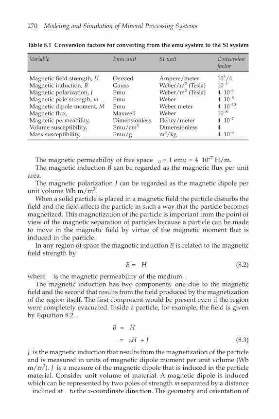
270 Modeling and Simulation of Mineral Processing Systems
The magnetic permeability of free space 0 = 1 emu = 4 10–7 H/m.The magnetic induction B can be regarded as the magnetic flux per unit
area.The magnetic polarization J can be regarded as the magnetic dipole per
unit volume Wb m/m3.When a solid particle is placed in a magnetic field the particle disturbs the
field and the field affects the particle in such a way that the particle becomesmagnetized. This magnetization of the particle is important from the point ofview of the magnetic separation of particles because a particle can be madeto move in the magnetic field by virtue of the magnetic moment that isinduced in the particle.
In any region of space the magnetic induction B is related to the magneticfield strength by
B = H (8.2)
where is the magnetic permeability of the medium.The magnetic induction has two components: one due to the magnetic
field and the second that results from the field produced by the magnetizationof the region itself. The first component would be present even if the regionwere completely evacuated. Inside a particle, for example, the field is givenby Equation 8.2.
B = H
= 0H + J (8.3)
J is the magnetic induction that results from the magnetization of the particleand is measured in units of magnetic dipole moment per unit volume (Wbm/m3). J is a measure of the magnetic dipole that is induced in the particlematerial. Consider unit volume of material. A magnetic dipole is inducedwhich can be represented by two poles of strength m separated by a distance inclined at to the x-coordinate direction. The geometry and orientation of
Table 8.1 Conversion factors for converting from the emu system to the SI system
Variable Emu unit SI unit Conversionfactor
Magnetic field strength, H Oersted Ampere/meter 103/4Magnetic induction, B Gauss Weber/m2 (Tesla) 10–4
Magnetic polarization, J Emu Weber/m2 (Tesla) 4 10–4
Magnetic pole strength, m Emu Weber 4 10–8
Magnetic dipole moment, M Emu Weber meter 4 10–10
Magnetic flux, Maxwell Weber 10–8
Magnetic permeability, Dimensionless Henry/meter 4 10–7
Volume susceptibility, Emu/cm3 Dimensionless 4Mass susceptibility, Emu/g m3/kg 4 10–3

Magnetic separation 271
the particle in relation to the magnetic field determines the angle and thedipole does not normally lie parallel to the vector J .
The effective moment parallel to the x-coordinate direction is m cos andis related to the x-component of J by
m J x cos = (8.4)
for unit volume of medium. Similar expressions can be written for the othercoordinate directions.
The magnetic polarization J is proportional to the field strength inside theparticle, H , and
J = 0 H (8.5)
where is the volume susceptibility of the material. The permeability andvolume susceptibility are not independent because
B = 0H + 0 H = 0(1 + )H (8.6)
and by comparison with Equation 8.2
= 0(1 + ) (8.7)
The relative permeability, r, of the material is given by
r = / 0 = 1 + (8.8)
Diamagnetic and paramagnetic materials have small negative and positivevalues of respectively and these are independent of the field strength H.Ferromagnetic materials have larger positive values of and in addition thesusceptibility, and hence the permeability, is a function of H. In fact inferromagnetic materials J does not continue to increase indefinitely as Hincreases but approaches a limiting value which is the familiar phenomenonof saturation.
Before discussing the magnetization of the particle, the disturbance of thefield by the particle must be considered. The magnetic permeability of theparticle will in general be different to that in the surrounding medium andthe magnetic field is distorted in the neighborhood of the particle. The extentof the distortion depends on the shape of the particle and the value of itspermeability. When the exterior field is uniform far from the particle, thefield inside the particle is uniform also and is directed parallel to the exteriorfield and in the same direction as shown in Figure 8.1. For a number ofdifferent particle shapes
H HN
= 1 +
(8.9)
whereH is the external magnetic field strength,H is the magnetic field strength inside the particle,
r is the relative permeability of the particle, and
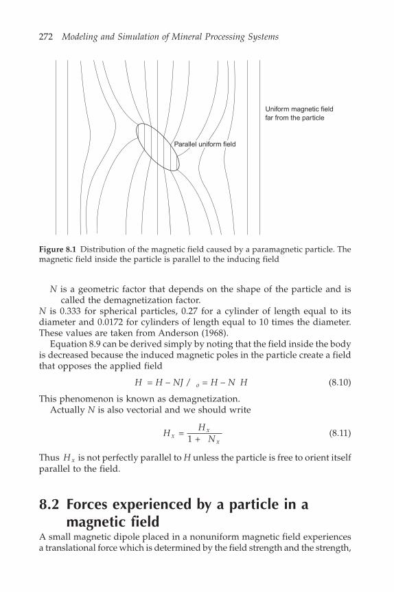
272 Modeling and Simulation of Mineral Processing Systems
Parallel uniform field
Uniform magnetic fieldfar from the particle
N is a geometric factor that depends on the shape of the particle and iscalled the demagnetization factor.
N is 0.333 for spherical particles, 0.27 for a cylinder of length equal to itsdiameter and 0.0172 for cylinders of length equal to 10 times the diameter.These values are taken from Anderson (1968).
Equation 8.9 can be derived simply by noting that the field inside the bodyis decreased because the induced magnetic poles in the particle create a fieldthat opposes the applied field
H = H – NJ / o = H – N H (8.10)
This phenomenon is known as demagnetization.Actually N is also vectorial and we should write
HH
Nxx
x =
1 + (8.11)
Thus H x is not perfectly parallel to H unless the particle is free to orient itselfparallel to the field.
8.2 Forces experienced by a particle in amagnetic field
A small magnetic dipole placed in a nonuniform magnetic field experiencesa translational force which is determined by the field strength and the strength,
Figure 8.1 Distribution of the magnetic field caused by a paramagnetic particle. Themagnetic field inside the particle is parallel to the inducing field
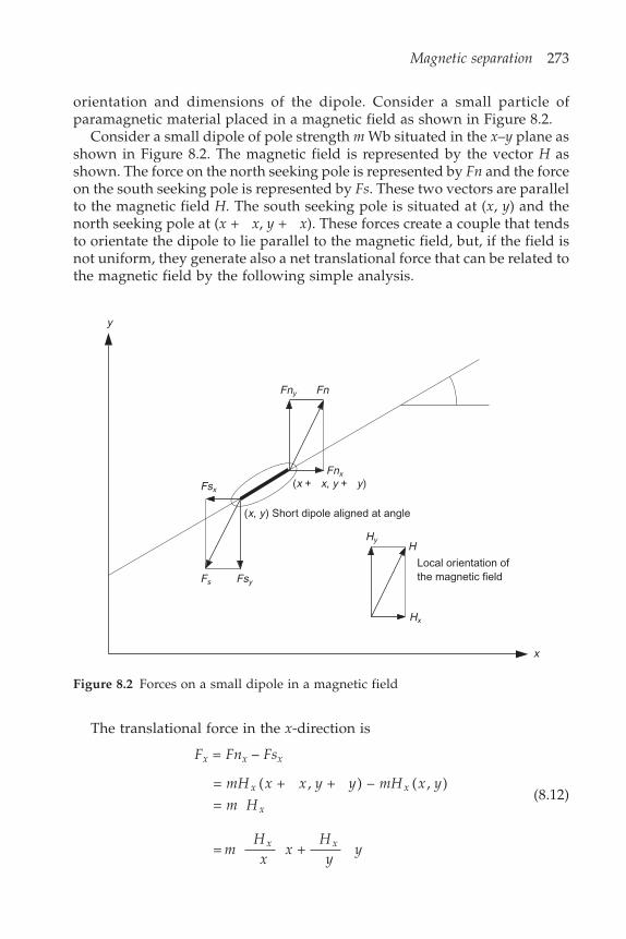
Magnetic separation 273
y
x
Fny Fn
Fnx
(x + x, y + y)
(x, y) Short dipole aligned at angle
Fsx
Fs Fsy
HyH
Hx
Local orientation ofthe magnetic field
orientation and dimensions of the dipole. Consider a small particle ofparamagnetic material placed in a magnetic field as shown in Figure 8.2.
Consider a small dipole of pole strength m Wb situated in the x–y plane asshown in Figure 8.2. The magnetic field is represented by the vector H asshown. The force on the north seeking pole is represented by Fn and the forceon the south seeking pole is represented by Fs. These two vectors are parallelto the magnetic field H. The south seeking pole is situated at (x, y) and thenorth seeking pole at (x + x, y + x). These forces create a couple that tendsto orientate the dipole to lie parallel to the magnetic field, but, if the field isnot uniform, they generate also a net translational force that can be related tothe magnetic field by the following simple analysis.
Figure 8.2 Forces on a small dipole in a magnetic field
The translational force in the x-direction is
Fx = Fnx – Fsx
= ( + , + ) – ( , )=
mH x x y y mH x y
m Hx x
x(8.12)
= + mHx
xHy
yx x
274 Modeling and Simulation of Mineral Processing Systems
If the dipole length is , x = cos and y = sin
F mHx
Hyx
x x = cos + sin (8.13)
Likewise the y-component of the translational force is given by:
F mHx
Hyy
y y = cos + sin (8.14)
Using Equation 8.4 these become:
F v JHx
v JHyx p x
xp y
x = + (8.15)
and
F v JHx
v JHyy p x
yp y
y = + (8.16)
where vp is the volume of the particle.This entire analysis can be extended to three dimensions in a straightforward
manner.When a small particle of magnetic susceptibility is placed in the magnetic
field, the induced magnetism in the particle creates the effective dipole moment.The magnetic moment per unit volume J in the particle is related to the field,H, by Equations 8.5 and 8.9.
JHN
= 1 +
0 (8.17)
Both J and H are vectors and, as Equation 8.17 implies, the induced magneticmoment J is parallel to the field H.
Substitution in Equation 8.15 gives:
Fv
NH
Hx
HHyx
px
xy
x = 1 +
+ 0
(8.18)
The components of the magnetic field strength can be written in terms of thegradient of a magnetic potential as follows:
Hx
Hy
x
y
= –
= –(8.19)
which yields the symmetry relationships:
Hx x y y x
Hy
y x = – = – = 2 2
(8.20)
Magnetic separation 275
and
Hy y x x y
Hx
x y = – = – =
2 2(8.21)
Thus
Fv
NH
Hx
HHxx
p
rx
xy
y =
1 + ( – 1) +
0(8.22)
This can be written:
Fv H
N xxp
= 0.5
1 + 0
2
(8.23)
where H H H Hx y z2 2 2 2 = + + is the square of the magnetic field strength.
Equivalent expressions can be derived for the y and z components of theforce experienced by the particle in the magnetic field.
If is the mass susceptibility of the particle and mp the mass of the particle
vp = mp (8.24)
= p (8.25)
where p is the density of the particle.Equation 8.22 shows clearly that the strength of translational force is
proportional to product of the magnetic field strength and its gradient.Consequently magnetic separators must be constructed so that high fieldscontaining strong field gradients are present. Methods for achieving this willbe discussed later.
The force can be written as a product of two factors:
Vv
Nmp
= 0.51 +
(8.26)
and
fm = 0 H2 (8.27)
Vm has the dimensions of m3 and is called the magnetic volume of the particle.fm has dimensions N/m3 and is called the magnetic force density. The valueof Vm is determined by the characteristics of the particles and is particlespecific. The magnetic force density is a function primarily of the machinedesign and magnetic field generated by the machine. It is therefore a machine-specific parameter. However, if the particles are subject to magnetic saturationin the working field, the magnetic force density will also be a function of thesaturation magnetization of the particle. The force acting a particle in a magneticfield is the product of Vm and fm.
F = Vmfm (8.28)
276 Modeling and Simulation of Mineral Processing Systems
The concept of magnetic volume of a particle is especially convenient forpractical calculations because the magnetic volume of a composite mineralparticle is the sum of the magnetic volumes of the separate components. Themagnetic volume of component i is calculated from
Vv v
Nmii p i
p =
0.51 +
(8.29)
where vi is the volume fraction of component i and vp and p are the volumeand magnetic susceptibility of the particle.
Illustrative example 8.1Calculate the radial component of the force on a small spherical paramagneticparticle of diameter 100 m in the neighborhood of a magnetically saturatedferromagnetic wire of radius a. The magnetic field has the following componentsin cylindrical coordinates.
H Ha
rHr s = + cos
2
2 0
H Ha
rHs = – sin
2
2 0
Hz = 0
Hs is the field inside the magnetically saturated wire and H0 is the strength ofthe magnetizing field.
Use the following data:
Hs = 2 103 A/m
H0 = 3 103 A/m
a = 1 mm
Magnetic susceptibility of the particle = 1.36 10–3
The particle is situated at coordinate location r = 1.05 mm and = 0
SolutionThe force on the particle is given by
Fv
NH
p =
0.51 +
0 2
where vector notation has been used to represent F and H.The square of the field strength is obtained from the components of the
field strength vector
H H H Hr z2 2 2 2 = + +

Magnetic separation 277
H Har
H Har
Hs s2
2
2 0
22
2
2 0
22 = + cos + – sin
The radial component of the force is given by
Fv
NH
rrp
= 0.51 +
02
Hr
Har
H H ar
Har
H H ar
s s s s
2 2
2 02
32
2
2 02
32 = – 4 + cos – 4 – sin
Hr
2 3
23
3
3 –3 = –42 10
1.05 + 3 10 2 10
1.05 10
Hr
210 = 3.327 10
The magnetic volume of the particle is:
Vm = 0.51 36 10 /6(100 10 )
1 + 0.3331 36 10
–3 –6 3
–3
= 3.559 10–16 m3
The magnetic force density is:
fH
rm = 0
2
= 4 10–7 3.327 1010 = 4.18 104 N/m3
The radial component of the force experienced by the particle is:
Fr = 3.559 10–16 4.18 104 = 1.49 10–11 N
Notice that this is a small force!
8.3 Magnetic properties of mineralsDifferences in magnetic susceptibilities between minerals may be exploitedfor their separation in a machine that will permit the particles to move underthe influence of the magnetic field according to Equation 8.22 and under theinfluence of some other field such as gravity or a shearing field in a flowingliquid. Particles with high susceptibilities will be influenced strongly by themagnetic field. Particles of different susceptibilities will follow different pathsunder the influence of the two interacting fields and can thus be physicallyseparated.
278 Modeling and Simulation of Mineral Processing Systems
Magnetic susceptibilities of minerals are difficult to measure and the valuesare strongly influenced by impurities. The susceptibilities of most mineralsare low (typically less than 10–7 kg–1) and very high fields and field gradientsare required to effect a useful separation. A comprehensive tabulation ofsusceptibilities of minerals is not available and in any case the same mineralfrom various sources can exhibit significant variations. Minute inclusions ofmagnetite for example will drastically affect the apparent susceptibility.
A brief tabulation is given in Table 8.2.
Table 8.2 Magnetic susceptibilities of minerals at 20 C (Lawver andHopstock, 1974)
Mineral Chemical composition (m3/kg)
Quartz SiO2 –6.19 10–9
Calcite CaCO3 –4.80 10–9
Sphalerite -ZnS –3.23 10–9
Pyrite FeS2 3.57 10–9
Hematite -F22O3 259 10–9
Goethite -FeOOH 326 10–9
Siderite FeCO3 123 10–8
Fayalite FeSiO4 126 10–8
Values for other minerals are given by Taggart (1945) and Gaudin (1939)but these values should be treated with caution. Svoboda (1987) gives acomprehensive summary of the available data on measured values of themagnetic susceptibility of minerals that can be separated by magnetic methods.
Effective values for magnetic susceptibilities may be obtained in the mineraldressing laboratory by use of the Franz isodynamic separator. The mineralmust be available as liberated particles and requires calibration with crystalsof known susceptibility.
8.4 Magnetic separating machinesProduction machines must operate continuously and the particles must movethrough the field in a continuous stream. Separation is effected by inducingthe particles of higher susceptibilities to take a path through the magneticfield, which will deflect them to the concentrate discharge ports. The magneticforces on most particles are very small and the high intensity regions of themagnetic field are small in extent. Consequently the machines must be designedto achieve a separation based on a comparatively weak effect which can onlyinfluence the particle for a short time during its passage through the machine.The mechanical design of magnetic separators is crucial to the effectivenessof their operation but the difficulty in relating the fundamental properties ofthe particle mechanics in magnetic fields to the detailed behavior of the

Magnetic separation 279
machines has hampered the development of machines capable of highselectivity and good recovery of minerals. That improvements can be effectedby the use of high magnetic fields is obvious and the improvements in wethigh intensity magnetic separators has led to a growing list of applicationsover recent years.
The basis of performance calculations for both wet and dry magneticseparators is given below. The use of wet magnetic separators is preferred inthe plant environment. Dry separators are limited to treating ores that can beliberated at particle sizes greater than 75 m. Very small particles are severelyinfluenced by air currents and tend to agglomerate and adhere to the polesurfaces of the machine. Machines that can handle slurries do overcomethese problems to a certain extent and also offer the advantage of eliminationof the drying stage when wet grinding is used.
8.4.1 Production of the magnetic fieldThe quantitative analysis presented above demonstrates that high gradientsin the magnetic field are required as well as high field strength if a significantforce is to act on weakly paramagnetic particles in the machine. Magneticfields are normally produced by electromagnets and the pole pieces designedto create the high field gradients. Designs vary considerably among the differentmanufacturers and only the general principles are described here.
The field is established between two pole pieces, one of which is considerablynarrower than the other so that the field intensity is greatest in its neighborhood.This concentration of the field produces the necessary gradient in the field toimpart the required force on the paramagnetic particles. Two configurationsare shown schematically in Figure 8.3.
A matrix of ferromagnetic material is used in wet high intensity magneticseparators rather than fixed or moving poles of the type shown above. Thematrix provides a high concentration of points of high field intensity and canbe made from small spheres, expanded metal sheet, ‘wedge-wire’ bars orgrooved metal plates.
The magnetic field is most conveniently produced by electromagnets ratherthan permanent magnets. The field strength of an electromagnet may beconveniently varied by varying the current. The calculation of the field strengthgenerated between the poles of an electromagnet can be done simply only ifthe geometry of the coil, the core, the poles and the air gap is very simple.Hughes (1956) presents a simple example. This simple method is based onthe concept of the magnetic circuit which is made up of the core and polepieces of the electromagnet and the air gaps in which the separating field isgenerated. The various parts of the circuit are in series or parallel and thecomplete circuit forms a ring. A schematic representation is shown in Figure8.4.
The magnetic circuit shown in Figure 8.4 can be regarded as consisting ofsix segments in series: the core, pole 1, air gap 1, the keeper, gap 2 and pole2. In order to relate the magnetic field strength in the gaps to the current in
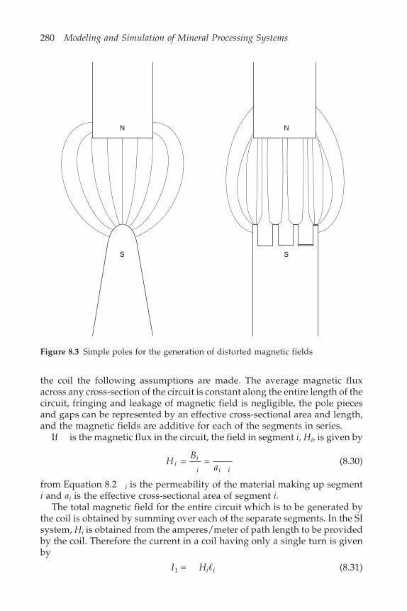
280 Modeling and Simulation of Mineral Processing Systems
N
S
N
S
the coil the following assumptions are made. The average magnetic fluxacross any cross-section of the circuit is constant along the entire length of thecircuit, fringing and leakage of magnetic field is negligible, the pole piecesand gaps can be represented by an effective cross-sectional area and length,and the magnetic fields are additive for each of the segments in series.
If is the magnetic flux in the circuit, the field in segment i, Hi, is given by
HB
aii
i i i = = (8.30)
from Equation 8.2 i is the permeability of the material making up segmenti and ai is the effective cross-sectional area of segment i.
The total magnetic field for the entire circuit which is to be generated bythe coil is obtained by summing over each of the separate segments. In the SIsystem, Hi is obtained from the amperes/meter of path length to be providedby the coil. Therefore the current in a coil having only a single turn is givenby
I1 = Hi�i (8.31)
Figure 8.3 Simple poles for the generation of distorted magnetic fields

Magnetic separation 281
Core
Coil
Pole 1 Pole 2g1 g2
Keeper
I
aii
i i1 =
�(8.32)
where �i is the effective length of segment I. The term �i/ai i is the magneticreluctance of segment i of the magnetic circuit.
Electromagnets are normally constructed with coils having many turns.The current required is reduced in proportion to number of turns so that
IInn = 1 (8.33)
is the current required in a coil having n turns.The average field strength in the gaps in Figure 8.4 is given by
Hag g
= (8.34)
H
nI a
an g g
i i i =
/
/�(8.35)
Figure 8.4 A simple magnetic circuit driven by an electromagnet
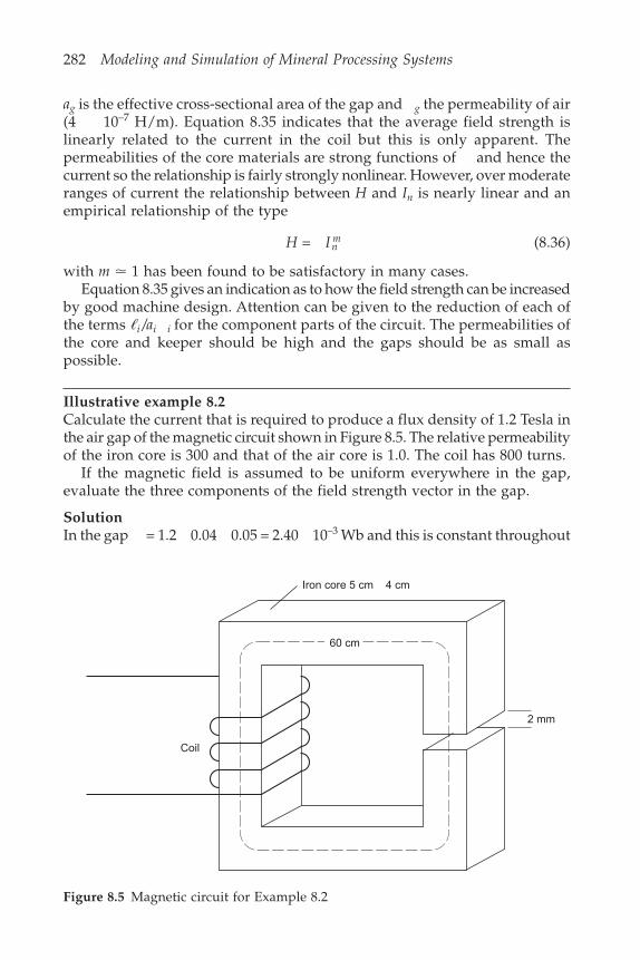
282 Modeling and Simulation of Mineral Processing Systems
Iron core 5 cm 4 cm
60 cm
Coil
2 mm
ag is the effective cross-sectional area of the gap and g the permeability of air(4 10–7 H/m). Equation 8.35 indicates that the average field strength islinearly related to the current in the coil but this is only apparent. Thepermeabilities of the core materials are strong functions of and hence thecurrent so the relationship is fairly strongly nonlinear. However, over moderateranges of current the relationship between H and In is nearly linear and anempirical relationship of the type
H Inm = (8.36)
with m � 1 has been found to be satisfactory in many cases.Equation 8.35 gives an indication as to how the field strength can be increased
by good machine design. Attention can be given to the reduction of each ofthe terms �i /ai i for the component parts of the circuit. The permeabilities ofthe core and keeper should be high and the gaps should be as small aspossible.
Illustrative example 8.2Calculate the current that is required to produce a flux density of 1.2 Tesla inthe air gap of the magnetic circuit shown in Figure 8.5. The relative permeabilityof the iron core is 300 and that of the air core is 1.0. The coil has 800 turns.
If the magnetic field is assumed to be uniform everywhere in the gap,evaluate the three components of the field strength vector in the gap.
SolutionIn the gap = 1.2 0.04 0.05 = 2.40 10–3 Wb and this is constant throughout
Figure 8.5 Magnetic circuit for Example 8.2
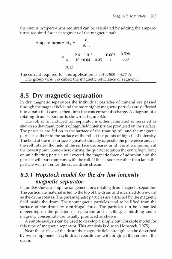
Magnetic separation 283
the circuit. Ampere-turns required can be calculated by adding the ampere-turns required for each segment of the magnetic path.
Ampere-turns = = nI
ani
i i
�
= 2.4 104 10 0.04 0.05
0.0021
+ 0.598300
–3
–7
= 3813
The current required for this application is 3813/800 = 4.77 A.The group �i/ai i is called the magnetic reluctance of segment I.
8.5 Dry magnetic separationIn dry magnetic separators the individual particles of mineral ore passedthrough the magnet field and the more highly magnetic particles are deflectedinto a path that carries them into the concentrate discharge. A diagram of arotating drum separator is shown in Figure 8.6.
The roll of an induced roll separator is either laminated or serrated asshown so that many points of high field intensity are produced on the surface.The particles are fed on to the surface of the rotating roll and the magneticparticles adhere to the surface of the roll at the points of high field intensity.The field at the roll surface is greatest directly opposite the pole piece and, asthe roll rotates, the field at the surface decreases until it is at a minimum atthe lowest point. Somewhere during the quarter rotation the centrifugal forceon an adhering particle will exceed the magnetic force of adhesion and theparticle will part company with the roll. If this is sooner rather than later, theparticle will not enter the concentrate stream.
8.5.1 Hopstock model for the dry low intensitymagnetic separator
Figure 8.6 shows a simple arrangement for a rotating drum magnetic separator.The particulate material is fed to the top of the drum and is carried downwardas the drum rotates. The paramagnetic particles are attracted by the magneticfield inside the drum. The nonmagnetic particles tend to be lifted from thesurface of the drum by centrifugal force. The particles can be separateddepending on the position of separation and a tailing, a middling and amagnetic concentrate are usually produced as shown.
A simple analysis can be used to develop a simple but workable model forthis type of magnetic separator. This analysis is due to Hopstock (1975).
Near the surface of the drum the magnetic field strength can be describedby two components in cylindrical coordinates with origin at the center of thedrum:
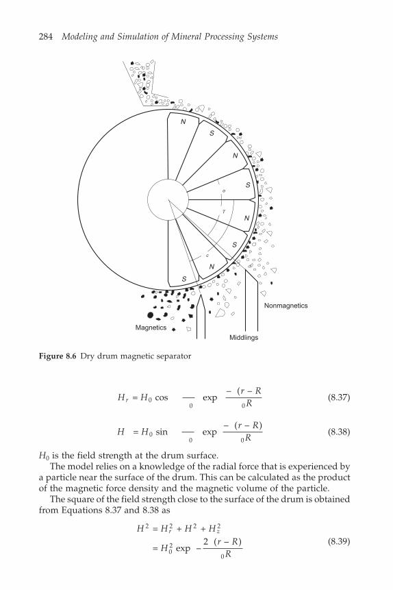
284 Modeling and Simulation of Mineral Processing Systems
N
N
S
S
N
S
N
S
c
T
o
Middlings
Magnetics
Nonmagnetics
H Hr R
Rr = cos exp – ( –
00 0
(8.37)
H Hr R
R = sin exp
– ( – )0
0 0(8.38)
H0 is the field strength at the drum surface.The model relies on a knowledge of the radial force that is experienced by
a particle near the surface of the drum. This can be calculated as the productof the magnetic force density and the magnetic volume of the particle.
The square of the field strength close to the surface of the drum is obtainedfrom Equations 8.37 and 8.38 as
H H H H
Hr R
R
r z2 2 2 2
02
0
= + +
= exp –2 ( – ) (8.39)
Figure 8.6 Dry drum magnetic separator

Magnetic separation 285
The radial component of force on a particle near the drum surface is given by:
F VH
r
V HR
r RR
r m
m
=
= –2
exp –2 ( – )
0
2
0 02
0 0
(8.40)
The negative sign indicates that the radial component of the force on aparamagnetic particle is directed inward.
At the surface of the drum, r = R and
F V HRr m = –
20 0
2
0(8.41)
The radial component of the magnetic force density at the surface of thedrum is:
fHRm =
2 0 02
0(8.42)
The behavior of a particle on the surface of the drum is governed by aforce balance.
The centrifugal force is given by:
FC = pvp2R (8.43)
and the radial component of the gravitational force is:
FGr = pvpg sin (8.44)
The particle will detach from the surface of the drum when
FC + FGr > Fr (8.45)
The critical rotation speed for detachment of a particle of magnetic volumeVm is obtained by equating the magnetic and centrifugal forces:
Crit0
0
/0 =
21
2Vv
HR
m
p p(8.46)
Because the ratio Vm /vp is independent of particle size, this model predictsthat the separating action of the rotating drum magnetic separator isindependent of particle size and this has been confirmed by experiment overa size range from about 1 mm to 6 mm.
The theoretical point of detachment of a particle magnetic volume Vm isgiven by
sin = –2
dm m
p p
V fv g
Rg
(8.47)

286 Modeling and Simulation of Mineral Processing Systems
In theory the drum separator should recover to tailing all particles that haveT < d and should recover to middling all particles that have T < d < 90 .
In practice the behavior of real materials in the magnetic separator deviatefrom the predicted pattern for a variety of reasons. Particle–particle interactionshave been neglected in the analysis and these can be significant in an industrialmachine because of the need to achieve economically high production ratesand that in turn dictates that the bed of particles on the drum must be severalmm thick. This will translate to a bed several layers thick if the particles aresmaller than about 1 mm. Significant variations in the magnetic field strengthon the surface of the drum caused by serrations and grooves or other designfeatures aimed at intensification of the gradients in the magnetic field areanother significant cause of imperfect behavior. In fact the value of the magneticforce density will be distributed over a range of values within the particlebed on the surface of the drum and the model should reflect this.
Imperfect separation of the desired mineral also results from the imperfectcorrelation between particle composition and the magnetic susceptibility ormagnetic volume of the particle. The conditional distribution density of Vmfor particles of mineral grade g can be quite wide and this should be reflectedin the model. If p( fm) is the distribution density for the magnetic force densitywithin the particle bed on the surface of the drum and p(Vm|g) is the conditionaldistribution of particle magnetic volume for particles of grade g, the yield totailing is given by:
YV f
v gR
gp f p V g p g df dV dgdT
m m
p pm m m m
T
= sin – ( ) ( | ) ( )0 0 0 0
–12
(8.48)
8.5.2 Capacity of the separatorThe tonnage handled by the rotating drum separator is given by:
Tonnage = R bb (8.49)
b = bulk density of layer.b = depth of bed.
Generally a bed depth equal to particle diameter is desirable but this mightlead to capacities that are too low. Then a depth of several particle layers willbe used. To increase tonnage, the drum should rotate at a rate close to thecritical value for separation of the lowest grade particle that should report tothe tailing.
Then
Tonnage = (1 + )
0
0
1/2
0bbN
H (8.50)
which is independent of R!
Magnetic separation 287
8.6 Wet high intensity magnetic separationDobby and Finch (1977) have developed an empirical model for the operationof the wet high intensity magnetic separator. The authors demonstrate thatrecovery of magnetic particles in a whims is dependent on the magneticsusceptibility and size of each particle. The probability of capture is proportionalto the ratio of the magnetic capture force and the hydrodynamic force thattends to dislodge the particle.
Fm = Magnetic force is proportional to d HG dp w3 /
G = H if H < Hs
or
G = Hs if H > Hs
Fu = Hydrodynamic force is proportional to dp uf
dw is the diameter of the matrix wire and Hs is the saturation magnetic fieldstrength within the matrix material. U is the average velocity of the slurry asit flows through the matrix.
The recovery of a particle of size dp and magnetic susceptibility shouldbe a function of the group
FF
d Hu
M
H
p =
2 2
(8.51)
Their experimental data are correlated better by the group
MHG d
u LL
p
m =
( )1.2 2.5
1.8 0.8 (8.52)
where
LM is the matrix loading =Mass fraction of magnetics in feed
Mass of matrix
The recovery of particles of size dp and volumetric magnetic susceptibility is modeled by
R d BMMM p
L( , ) = 0.5 + log1050
for M5010–0.5/B ML M50100.5/B
= 0 for ML < M5010–0.5/B (8.53)
= 1.0 for ML > M50100.5/B
M50 is the magnetic cut point at which the recovery is 0.5. M50 and B areparameters that are specific to a particular machine but independent of thematerial that is treated. Dobby and Finch found B = 0.348 and M50 = 1.269 10–2 for the machine that they tested.
288 Modeling and Simulation of Mineral Processing Systems
The particle population in the feed to the magnetic separator will bedistributed over a range of values of and dp so that the total yield of solidsto magnetics is given by
Y R g d p g d p d R d p di j m p ij p j p j p p j p = ( ), ) ( | ) ( ) + ( ) ( )( (8.54)
where R(dp) is the fractional retention of particles of size dp by physicalentrapment. In practice it is easier to measure the distribution of magneticsusceptibilities in a sample of the feed material directly in a laboratoryexperiment using the isodynamic separator or rotating drum separator andthen to determine the average value of the grade g for each of the separatedfractions. The distribution of particle grades in each magnetic fraction can bedetermined by image analysis techniques. In that case the yield to magneticsis given by
Y R d p g d p g d p dk i j M p kij p ij p j p = , ) ( | , ) ( | ) ( )( (8.55)
with
pkij( |g, dp) pij(g|dp) = pikj(g| ! dp)pkj( |dp) (8.56)
BibliographyMagnetic separation methods are comprehensively surveyed in books bySvoboda (1987) and Gerber and Birss (1983).
ReferencesAnderson, J.C. (1968) Magnetism and Magnetic Materials. Chapman and Hall Ltd, London,
p. 24.Dobby, G. and Finch, J.A. (1977) An empirical model of capture in a high gradient
magnetic separator and its use in performance prediction. XIIth Int. Min. Proc.Congr., Sao Paulo, Brazil, Special Publication, Vol. I, pp. 128–152.
Gaudin, A.M. (1939) Principles of Mineral Dressing. McGraw-Hill, New York, p. 436and p. 438.
Gerber, R. and Birss, R.R. (1983) High Gradient Magnetic Separation. Research StudiesPress, Chichester.
Hopstock, D.M. (1975) Fundamental aspects of design and performance of low-intensitydry magnetic separators. Trans SME 258, pp. 221–227.
Hughes, E. (1956) Fundamentals of Electrical Engineering. Longmans Green and Co.,London, p. 47.
Lawver, J.E. and Hopstock, D.M. (1974) Wet magnetic separation of weakly magneticmaterials. Minerals Sci. Engng, Vol. 6, pp. 154–172.
Svoboda, J. (1987) Magnetic Methods for the Treatment of Minerals. Elsevier, Amsterdam.Taggart, A.F. (1945) Handbook of Mineral Dressing. John Wiley and Son, pp. 13–17.
9Flotation
Flotation is the most widely used mineral separation method. It is the preferredmethod of mineral recovery for many of the most important minerals that arerecovered and large tonnages of ore are processed by flotation annually.
The underlying principles of the flotation process are well established butit has proved to be unusually difficult to build quantitative predictive modelsthat can be used to simulate the operation of flotation cells in typical industrialcircuits. The reason for the difficulty lies in the complexity of the many microprocesses that combine to produce the overall result, which is the separationof different mineral species by virtue of the differential surface conditionsthat can be induced on the various minerals. In the flotation cell, an agitatedslurry is aerated by introducing a cloud of air bubbles that are typically abouta millimeter in size. The agitation of the slurry is sufficient to keep the solidparticles in suspension although the suspension is usually not uniform, withthe larger heavier particles tending to remain in the lower parts of the cell.
The rising bubbles can and do collide with the suspended solid particlesand those particles that have appropriate surface characteristics can attach toa rising bubble and can therefore be carried upward, eventually reaching thesurface of the slurry. Each bubble will have many encounters with particlesduring its rise through the slurry and a bubble can carry several particles tothe top of the slurry.
A more or less stable layer of froth is maintained on the surface of theslurry. Particles that are attached to bubbles will tend to remain attached atair–water interfaces when the bubble enters the froth layer. Particles that areretained in the froth are recovered at the lip of the froth weir at the edge ofthe flotation cell. The recovery of the froth is accomplished by the naturalmobility of the froth, which causes it to flow over the weir, and the recoveryis sometimes assisted by mechanical paddles.
Within this general macroscopic view of the flotation process as a whole,several distinct micro processes can be identified. Each of these plays a rolein determining how individual solid particles will respond while they are ina flotation cell. Prior to any flotation taking place, a number of detailedchemical processes occur on and exceedingly close to the surfaces of theparticles. This is a chemical conditioning step and it is necessary in order toensure that differential hydrophobicity is achieved with respect to the differentmineral species that are present. Minerals that have strongly hydrophobicsurfaces have a greater chance of recovery into the froth phase than particlesthat are weakly hydrophobic or hydrophilic. The chemical conditioning ofmineral surfaces for flotation has been the subject of sustained research efforts
290 Modeling and Simulation of Mineral Processing Systems
for the best part of a century and a great deal is known about the surfacechemistry and the role the chemical factors play in the aqueous phase and onthe particle surfaces. However most of this understanding is qualitative withcomparatively little information emerging that allows quantitative predictionof such important variables as contact angle and other measures ofhydrophobicity. As a result, quantitative models of flotation cell performancedo not at present make any significant use of quantitative chemical parameterssuch as for example the pH of the slurry and the concentration of chemicalcollectors or frothers to define overall process behavior. Hopefully the situationwill change in the future and an understanding of the surface chemistry willplay its appropriate role in the development of truly predictive quantitativemodels for flotation.
Much the same can be said for the froth phase. Although a great deal isknown about the structure of froths and foams, it is not possible to makequantitative predictions about froth stability and froth mobility and theireffect on the ability to hold and ultimately recover mineral particles thatenter the froth attached to bubbles.
When formulating a quantitative model for the flotation process, it isnecessary to start from the premise that, by virtue of appropriate chemicalconditioning of the slurry, minerals will exhibit varying levels of surfacehydrophobicity, and, consequently, a separation of particles is possible, basedon the proportion of different mineral exposure on the surface. Likewise it ispresumed that a more or less stable and mobile layer of froth will persist onthe surface of the slurry that will gather and recover a proportion of theadhering mineral particles.
9.1 A kinetic approach to flotation modelingAlmost all successful models of the flotation process have been based on thepremise that flotation is a kinetic process. In this way a model can be formulatedin terms of a rate of flotation, which can be quantified in terms of some of themany chemical and physical factors that define the environment inside aflotation cell. The formulation of a suitable rate model is not straightforwardand it must be based on an analysis of the individual subprocesses that affectan individual particle in the flotation environment. These subprocesses canbe identified by noting that a particle must successfully complete the followingsteps in order to be recovered in the froth phase of a flotation cell:
1. The particle must achieve a level of hydrophobicity that will permit itto attach to a rising bubble.
2. The particle must be suspended in the pulp phase of the cell.3. The particle must collide with a rising bubble.4. The particle must adhere to the bubble.5. The particle must not detach from the bubble during passage through
the pulp phase.
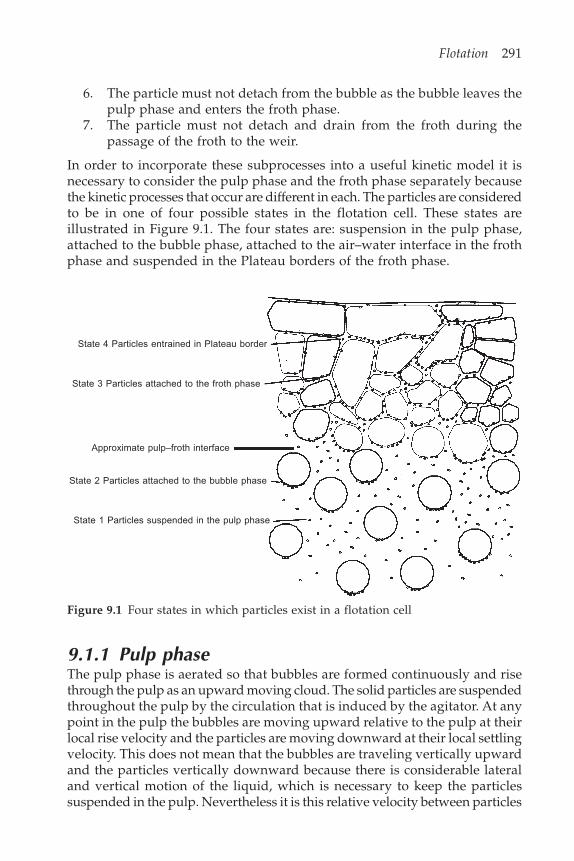
Flotation 291
6. The particle must not detach from the bubble as the bubble leaves thepulp phase and enters the froth phase.
7. The particle must not detach and drain from the froth during thepassage of the froth to the weir.
In order to incorporate these subprocesses into a useful kinetic model it isnecessary to consider the pulp phase and the froth phase separately becausethe kinetic processes that occur are different in each. The particles are consideredto be in one of four possible states in the flotation cell. These states areillustrated in Figure 9.1. The four states are: suspension in the pulp phase,attached to the bubble phase, attached to the air–water interface in the frothphase and suspended in the Plateau borders of the froth phase.
State 4 Particles entrained in Plateau border
State 3 Particles attached to the froth phase
Approximate pulp–froth interface
State 2 Particles attached to the bubble phase
State 1 Particles suspended in the pulp phase
Figure 9.1 Four states in which particles exist in a flotation cell
9.1.1 Pulp phaseThe pulp phase is aerated so that bubbles are formed continuously and risethrough the pulp as an upward moving cloud. The solid particles are suspendedthroughout the pulp by the circulation that is induced by the agitator. At anypoint in the pulp the bubbles are moving upward relative to the pulp at theirlocal rise velocity and the particles are moving downward at their local settlingvelocity. This does not mean that the bubbles are traveling vertically upwardand the particles vertically downward because there is considerable lateraland vertical motion of the liquid, which is necessary to keep the particlessuspended in the pulp. Nevertheless it is this relative velocity between particles

292 Modeling and Simulation of Mineral Processing Systems
and bubbles that is primarily responsible for collisions between particles andbubbles.
Particles can leave the pulp phase through one of two routes: by collisionwith and attachment to a bubble or direct to the froth phase by entrainmentat the pulp–froth interface. The collision and attachment subprocesses arediscussed in some detail later in this chapter and they govern, to a largeextent, the kinetic behavior of the particles in a flotation cell.
Particles can re-enter the pulp phase by detachment from a bubble or bydraining from the Plateau borders in the froth.
9.1.2 Bubble phaseThe bubble phase consists of a cloud of bubbles that rise through the pulpphase. A particle transfers from the pulp phase to the bubble phase by aprocess of bubble–particle collision and particle attachment. Once a particleis attached to a bubble it moves with the bubble and eventually it will reachthe froth phase unless it is detached from the bubble, in which case it returnsto the pulp phase. Bubbles become steadily more and more heavily loadedwith attached particles as the bubble passes through the pulp.
9.1.3 Froth phaseParticles enter the froth phase when a bubble carrying the particles crossesthe pulp–froth interface. The froth phase floats on top of the pulp phase andis formed by the bubbles that break through the surface of the pulp phase.The water in the flotation cell is conditioned to promote the formation of amore or less stable froth. The bubbles do not burst when they cross theinterface and each one carries a skin of water into the froth phase. The bubblesmove close together, with a single film of liquid separating the individualbubbles. When the bubbles are small, these boundary films are curved. Theliquid drains from the films, which become thinner and eventually breakcausing adjacent bubbles to coalesce. The bubbles become larger and largerand polyhedral in shape. At the junction of the polyhedral edges of the bubbles,Plateau borders form which act as a network of more or less tubular conduitsthrough which the draining liquid can move downward. The particles thatremain attached to the surface of bubbles in the froth move with the frothuntil they are eventually recovered in the concentrate froth when it passesover the froth lip of the flotation cell. Particles can become detached from theliquid film and transfer from the froth phase to the Plateau borders in thefroth from where they can drain back into the pulp phase.
9.1.4 Entrained phaseParticles are entrained in the Plateau borders of the froth and will tend tosettle down toward the pulp–froth interface under the influence of gravity.This settling is assisted further by the draining of the water as the filmsbetween bubbles in the froth become thinner and possibly break. This water
Flotation 293
flows through the network of Plateau borders and eventually re-enters thepulp phase. Particles enter the entrained phase by detachment from the air-water surfaces in the froth and also by direct entrainment from the pulpphase immediately below the pulp–froth interface on the top of the pulp.
9.2 A kinetic model for flotationThe kinetic model for flotation is based on the following simple principle. Asingle bubble rising upward through the pulp phase will collide with suspendedparticles and some of these particles will attach to the bubble surface and willtravel upward with the bubble. The rate at which bubbles collide with particlesdepends on the size of the bubbles and the size of the particles, their relativevelocities, and the concentration of particles in the pulp. The number ofparticles that can collide with the bubble can be calculated in the followingway.
The volume of pulp that is swept by a bubble per second is 4
2D Ubh b where
Ub is the local rise velocity of the bubble and Dbh the bubble diameter projectedon to the horizontal plane. This is generally different to the volume equivalentbubble diameter Dbe because a rising bubble distorts into an ellipsoidal shapeunless it is very small.
A population balance approach is taken so that the population of particlesin the cell is conceptually divided into classes so that particles in any oneclass are all similar in size and composition. The number of potential collisionswith the particles of type ij is proportional to the concentration Cij of theseparticles in the pulp phase. The diameter of the swept volume from which aparticle of size dpi may be captured is Dbh + dpi. The number of potentialcollisions with particles of size dpi is given by:
Number of potential collisions with particles of type
ij D d U v Cbh pi b Tij ij = 4
( + ) ( + )2 (9.1)
where Ub is the velocity of rise of the bubble and vTi is the free fall velocity ofthe particle. These are taken to be the terminal velocities in the gravitationalfield in both cases, although in the turbulent circulating flow inside a flotationcell, terminal velocities may not be achieved by all particles and bubbles.
The rate of transfer of particles from the pulp phase to the bubble phase(transitions from state 1 to state 2 in Figure 9.1) is given by
Ideal rate of transfer = number of potential collisions number of bubbles/unit volume
=4
( + ) ( + )
6
kg/m of cell volume2
3
3D d U v CG
Dbh pi b Tij ij
v b
be
(9.2)
where Gv is the specific aeration rate in m3 air/s m3 cell volume and b is the
294 Modeling and Simulation of Mineral Processing Systems
average bubble residence time in the cell. Dbe is the effective spherical diameterof the bubble.
In a real flotation cell, this ideal rate of transfer is never achieved becausenot all of the potential collisions actually occur and, of those that do occur,not all are successful in achieving adhesion between the bubble and theparticle. The ideal rate is accordingly modified to reflect these inefficiencies.
Rate of transfer
= 32
( + ) ( + ) (1 – ) kg/m of cell23
3D d U v CGD
E E Ebh pi b Tij ijv b
beCij Aij Dij
(9.3)
where ECij is the fraction of particles that are in the path of the bubble whichactually collide with it. EAij is the fraction of bubble–particle collisions thatlead to successful attachment.
EDij is the fraction of particles of type ij that are detached from the bubbleduring the time that it takes the bubble to rise through the pulp phase. Thedevelopment of a quantitative kinetic model for the flotation process startswith models for ECij, EAij, and EDij.
The subprocesses of collision, attachment and detachment can be consideredto be independent since they are governed by essentially different forces. Thecollision process is dominated by the local hydrodynamic conditions aroundthe bubble. The attachment process is dominated by the short-range surfaceforces and by the drainage and rupture characteristics of the thin liquid filmbetween the bubbles and contacting particles. The detachment process isgoverned by stability considerations of the multi-particle aggregates that areformed on the bubble surface following successful attachment of the particles.These processes are largely independent of each other and, as will be shownbelow, require different models for their quantitative description.
The efficiency of bubble capture is reduced by the presence of other adheringparticles which cover a portion of the bubble surface area. A necessary resultof this kinetic model is that any bubble will become progressively coveredwith attached particles during its passage through the pulp phase. This behaviorhas been confirmed by direct experimental observation and is clearly shownin the photographic sequence in Figure 9.2. These photographs of a singlebubble were taken to record the increasing load of particles during the lifetimeof the bubble in the pulp. The essential elements of the collection of particlesby bubbles are clearly illustrated in these photographs. The sweeping actionof the fluid motion, which makes the particles slide over the bubble andaccumulate on the lower surface, is strikingly evident. This behavior influencesboth the collision efficiency Ec and the adhesion efficiency EA.
9.2.1 Particle–bubble collisionsNot every particle in the path of a rising bubble will collide with the bubblebecause, as the bubble advances through the water, it forces the water aside

Flotation 295
and this tends to carry the particles out of the path of and around the bubble.The processes that are at work can be seen in Figure 9.3, which shows thestreamlines that are formed around a bubble as it advances through the pulp.The streamlines shown in Figure 9.3 were calculated for two extreme flowregimes: Stokes flow, which applies when the bubble Reynolds number isvery much less than unity, and potential flow, which applies when the bubbleReynolds number is very much larger than unity. The streamlines show thetrajectories that a small neutrally buoyant particle will take during the encounterwith the bubbles. Such a particle will collide with the bubble only if it is ona streamline that has its closest approach to the bubble less than or equal tothe radius of the particle. The streamlines shown in Figure 9.3 were calculatedso that they are uniformly distributed a long way in front of the bubble. Thismeans the two sets of streamlines are directly comparable and it is easy to seethat the choice of flow model will have a significant effect on the value of Ec.Potential flow leads to much higher collision efficiencies than Stokes flow.
It can be seen from Figure 9.3 that a neutrally buoyant particle of diameterdp = 0.1 Db must be no more than about 17% of a bubble radius off the centerline of the collision path if it is to make contact with the bubble surfaceduring the flypast under Stokes flow. On the other hand a neutrally buoyantparticle of the same size would touch the bubble surface if it were as far outas 56% of the bubble radius under potential flow conditions. Obviously the
Figure 9.2 Loading of a single bubble during flotation. (a) After 3 seconds. (b) After10 seconds. (c) After 30 seconds. (d) After 125 seconds (King et al., 1974)
(c) (d)
(a) (b)
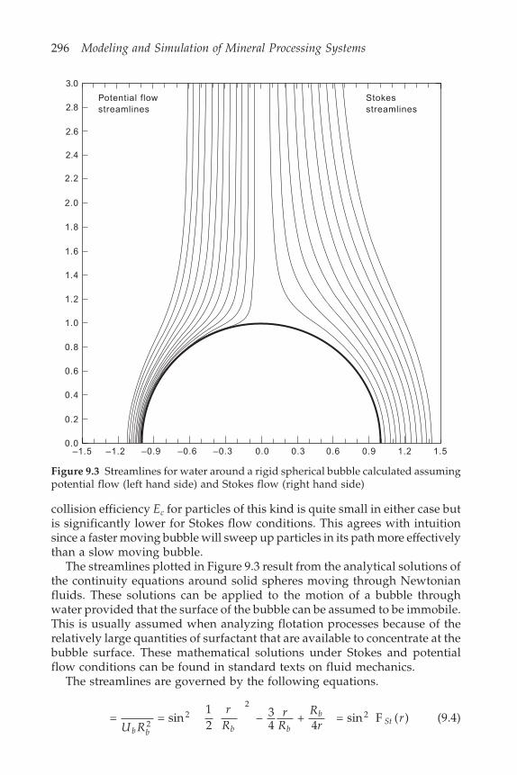
296 Modeling and Simulation of Mineral Processing Systems
collision efficiency Ec for particles of this kind is quite small in either case butis significantly lower for Stokes flow conditions. This agrees with intuitionsince a faster moving bubble will sweep up particles in its path more effectivelythan a slow moving bubble.
The streamlines plotted in Figure 9.3 result from the analytical solutions ofthe continuity equations around solid spheres moving through Newtonianfluids. These solutions can be applied to the motion of a bubble throughwater provided that the surface of the bubble can be assumed to be immobile.This is usually assumed when analyzing flotation processes because of therelatively large quantities of surfactant that are available to concentrate at thebubble surface. These mathematical solutions under Stokes and potentialflow conditions can be found in standard texts on fluid mechanics.
The streamlines are governed by the following equations.
= = sin
12
– 34
+ 4
= sin ( )22
22
U R
rR
rR
Rr
rb b b b
bStF (9.4)
Figure 9.3 Streamlines for water around a rigid spherical bubble calculated assumingpotential flow (left hand side) and Stokes flow (right hand side)
3.0
2.8
2.6
2.4
2.2
2.0
1.8
1.6
1.4
1.2
1.0
0.8
0.6
0.4
0.2
0.0–1.5 –1.2 –0.9 –0.6 –0.3 0.0 0.3 0.6 0.9 1.2 1.5
Potential flowstreamlines
Stokesstreamlines
Flotation 297
for Stokes flow and
= = sin
12
–2
= sin ( )22
22
PotU R
rR
Rr
rb b b
b F (9.5)
for potential flow. r and are the spherical spatial coordinates with the bubblecenter as origin. Ub is the velocity of rise of the bubble and Rb is the radius ofthe bubble.
Neither of the two extreme flow regimes, Stokes or potential flow, will beapplicable under all conditions in operating flotation cells and a model isrequired that will hold for all values of the bubble Reynolds from low (Stokesregime) to high (potential flow). Using published streamline patterns forrigid spheres moving in fluids over a range of bubble Reynolds numbers asa guide, Yoon and Luttrell (1989) used a weighted sum of the Stokes andpotential flow solutions to describe the streamlines around a sphere at Reynoldsnumbers in the range from 0 to 100.
= sin2 ( F st(r) + (1 – )F Pot(r)) = sin2 F (r) (9.6)
with F (r) given by
F ( ) = 1
2– 3
4 +
34
–12
2
rr
Rr
RRrb b
b (9.7)
is a dimensionless parameter that depends on the bubble Reynolds numberand has the value 1 when Reb = 0 (Stokes regime) and asymptotes to the value0 at high Reb (potential flow). also depends on the value of r. For values ofr only slightly larger than Rb, is close to unity.
is related to the bubble Reynolds number by:
= exp –4
45– 10.72Re rr
b (9.8)
where r = (r/Rb) and Rp is the radius of the particle.The bubble Reynolds number Reb = (DbUb w/ w) can be calculated from
the terminal rise velocity given the bubble size and the load of solids that itcarries (see Section 9.5).
9.2.2 A model for collision efficienciesThe collision efficiency is calculated as the fraction of the particles which arein the path of the bubble that actually collide with the bubble. In order to findwhich particles collide with the bubble, it is helpful to establish the streamlinesfor the particle motion since particles will deviate from the fluid streamlinesthat are shown in Figure 9.3. Particles deviate from the fluid streamlinesbecause they fall relative to the fluid as a result of their greater density andbecause inertia prevents the particle from accelerating at the same rate as the
298 Modeling and Simulation of Mineral Processing Systems
fluid when the fluid deviates from a straight line path as it approaches abubble.
The radial and azimuthal components of the fluid velocity are given by:
u
r
U R
rrr
b b = – 1 sin
= – 2 cos ( )2
2
2 F� (9.9)
u
r rU R
rrb b = 1
sin = cos ( )
2
F (9.10)
If the inertia of the particles is neglected, the particles move relative to thefluid at their terminal settling velocities, vT. Terminal settling velocities canbe calculated using the method described in Section 4.5. Then the componentsof the particle velocity vector are given by:
vr = ur – vT cos (9.11)
and
v = u + vT sin (9.12)
The stream function for the particle motion is therefore
p b b
T
b bU R r
vU
rR
= sin ( ) + 12
2 22
F (9.13)
The streamlines for water calculated using Equation 9.6 and the trajectoriesof particles having terminal settling velocity equal to 0.1Ub, calculated usingEquation 9.13, are shown in Figure 9.4 for a bubble rising with a Reynoldsnumber of 20.
The collision efficiency for particles of type ij is calculated as the flux ofparticles crossing an imaginary hemisphere of radius Rb + Rp that shrouds thefront hemisphere of the bubble divided by the flux of particles that cross ahorizontal plane of area (Rb + Rp)2.
Therefore
Ev R R R R d
R R U vCij
r r R R b p b p
b p b Tij
b p
= –2 | ( + ) sin ( + )
( + ) ( + )0
2= +
2
=
2 ( + )
( + ) +
+
2
2
U R R R
R Rv
U v
b b b p
b pTij
b Tij
F
(9.14)
Collision efficiencies can be measured in the laboratory using single bubbleflotation experiments with particles that are conditioned to be extremelyhydrophobic. These particles have adhesion efficiencies of 1.0 and the measuredcollection efficiency is therefore equal to the collision efficiency. The collision
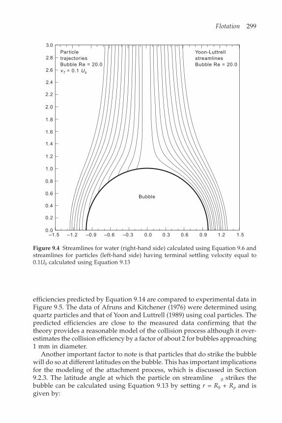
Flotation 299
efficiencies predicted by Equation 9.14 are compared to experimental data inFigure 9.5. The data of Afruns and Kitchener (1976) were determined usingquartz particles and that of Yoon and Luttrell (1989) using coal particles. Thepredicted efficiencies are close to the measured data confirming that thetheory provides a reasonable model of the collision process although it over-estimates the collision efficiency by a factor of about 2 for bubbles approaching1 mm in diameter.
Another important factor to note is that particles that do strike the bubblewill do so at different latitudes on the bubble. This has important implicationsfor the modeling of the attachment process, which is discussed in Section9.2.3. The latitude angle at which the particle on streamline 0 strikes thebubble can be calculated using Equation 9.13 by setting r = Rb + Rp and isgiven by:
Bubble
ParticletrajectoriesBubble Re = 20.0vT = 0.1 Ub
3.0
2.8
2.6
2.4
2.2
2.0
1.8
1.6
1.4
1.2
1.0
0.8
0.6
0.4
0.2
0.0–1.5 –1.2 –0.9 –0.6 –0.3 0.0 0.3 0.6 0.9 1.2 1.5
Yoon-LuttrellstreamlinesBubble Re = 20.0
Figure 9.4 Streamlines for water (right-hand side) calculated using Equation 9.6 andstreamlines for particles (left-hand side) having terminal settling velocity equal to0.1Ub calculated using Equation 9.13
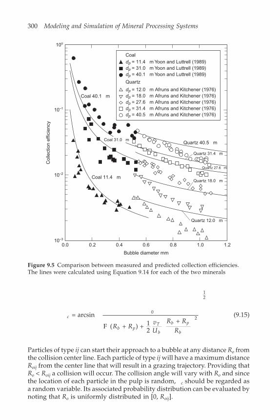
300 Modeling and Simulation of Mineral Processing Systems
c
b pT
b
b p
bR R
vU
R RR
= arcsin
( + ) + 12
+ 0
2
12
F
(9.15)
Particles of type ij can start their approach to a bubble at any distance Ro fromthe collision center line. Each particle of type ij will have a maximum distanceRoij from the center line that will result in a grazing trajectory. Providing thatRo < Roij a collision will occur. The collision angle will vary with Ro and sincethe location of each particle in the pulp is random, c should be regarded asa random variable. Its associated probability distribution can be evaluated bynoting that Ro is uniformly distributed in [0, Roij].
dp = 11.4 m Yoon and Luttrell (1989)dp = 31.0 m Yoon and Luttrell (1989)dp = 40.1 m Yoon and Luttrell (1989)
Quartz
dp = 12.0 m Afruns and Kitchener (1976)dp = 18.0 m Afruns and Kitchener (1976)dp = 27.6 m Afruns and Kitchener (1976)dp = 31.4 m Afruns and Kitchener (1976)dp = 40.5 m Afruns and Kitchener (1976)
Coal
100
10–1
10–2
10–3
0.0 0.2 0.4 0.6 0.8 1.0
Coal 40.1 m
Coal 11.4 m
Quartz 12.0 m
Quartz 18.0 m
Quartz 27.6 m
Quartz 40.5 m
Quartz 31.4 m
Coal 31.0 m
1.2
Col
lect
ion
effic
ienc
y
Bubble diameter mm
Figure 9.5 Comparison between measured and predicted collection efficiencies.The lines were calculated using Equation 9.14 for each of the two minerals

Flotation 301
Ro can be related to po by noting that far out from the bubble
sin = Rro (9.16)
so that Equation 9.13 gives
RU vo
po
b Tij =
2 +
12
(9.17)
and
RU voij
poij
b Tij =
2 +
12
(9.18)
where poij is the value of the particle stream function for the streamline thatrepresents the grazing trajectory for a particle of type ij at the equator of thebubble. This is evaluated using Equation 9.13 with = /2 and r = Rb + Rpij
.
oij b pij
Tij
b
b pij
bR R
vU
R RR
= ( + ) + 12
+ 2
F (9.19)
Substitution of Equations 9.17, 9.18 and 9.19 into Equation 9.15 gives a simplerelationship between c and Ro.
sin = co
oij
RR
(9.20)
By noting the uniform probability distribution of the random variable Ro, thedistribution density for the collision angle c is:
f c c c( ) = cos (9.21)
The corresponding cumulative distribution function for c is:
F c c c c( ) = sin for 0 2 (9.22)
9.2.3 Particle–bubble attachmentThe attachment process requires significantly more complex modeling thanthe collision process, which, as shown in the previous section, is governedprimarily by the fluid dynamics close to the bubble. The attachment processis governed by hydrodynamic and chemical factors which interact in complexways that ultimately determine whether a particle will attach to the bubbleor not.
When a particle collides with the bubble, the particle cannot immediatelyattach to the bubble because a thin film of liquid between the particle and thebubble must first drain. When the intervening film becomes sufficiently thinit can rupture allowing the particle to penetrate the skin of the bubble. The
302 Modeling and Simulation of Mineral Processing Systems
three-phase contact line that defines the penetration boundary of the bubblearound the particle must then develop to a stable configuration that is governedprimarily by the contact angle (both receding and advancing) of the solid andalso by its shape. Although the actual rupture step is very rapid the filmthinning and movement of the three-phase contact line are governed by kineticprocesses and each requires a finite time. The time taken from the instant ofcollision to the establishment of a stable three-phase contact is called theinduction time, which will be represented by tind. The induction time for aparticle is determined primarily by its contact angle but the particle size andshape are also important. Other chemical factors such as the concentration ofsurfactants at the bubble surface and the interaction between collector adsorbedon the solid and frother on the bubble surface also play a role. Purely physicalfactors such as the precise orientation of the particle on first contact and thevelocity profile close to the bubble surface and surrounding bubble all contributeto this enormously complex phenomenon. A detailed understanding of theseeffects has not yet been developed to the stage where induction times forirregular particles with heterogeneous surfaces can be confidently calculated.However, in general, particles with larger contact angles have shorter inductiontimes than similar particles having smaller contact angles. This variation ininduction time is the origin of the differential behavior of particles duringflotation and consequently it must form the kernel of any quantitative modelof flotation.
While the film thinning, film rupture and receding three-phase contactline are proceeding, another purely physical process is occurring. The particleis being carried downward over the surface of the bubble by the water as itmoves past the bubble surface. Particles against or attached to the bubble arewashed to the rear of the bubble. If a stable three-phase contact has beenestablished before the fluid streamlines start to diverge from the bubble,successful attachment is achieved and the particle remains attached to thebubble and continues its journey over the bubble surface until it collides withother particles already attached to the bubble which covers its lower pole.The accumulating collection of particles on the lower surface gradually buildsup until the whole of the lower hemisphere of the bubble is covered withadhering particles.
Particles that have not formed a stable three-phase contact by the time thestreamlines start to diverge from the bubble surface at the equator are pulledaway from the bubble surface and they do not attach. The time taken by aparticle to slide over the bubble surface from its point of collision to the pointof divergence is called the sliding time, ts. The fundamental principle thatgoverns the collision model of flotation is that a particle of size dp andcomposition g will attach to a bubble of size Rb only if it experiences a successfulcollision and its induction time is less than the sliding time.
tind ts (9.23)
This should properly be referred to as the Sutherland principle in recognitionof his pioneering attempt to put the understanding of flotation principles on
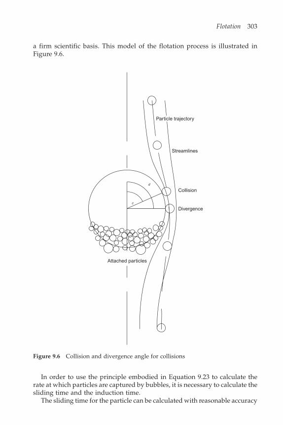
Flotation 303
Particle trajectory
Streamlines
Collision
Divergence
Attached particles
c
d
a firm scientific basis. This model of the flotation process is illustrated inFigure 9.6.
Figure 9.6 Collision and divergence angle for collisions
In order to use the principle embodied in Equation 9.23 to calculate therate at which particles are captured by bubbles, it is necessary to calculate thesliding time and the induction time.
The sliding time for the particle can be calculated with reasonable accuracy
304 Modeling and Simulation of Mineral Processing Systems
from a knowledge of the hydrodynamics in the water close to the bubblesurface. The tangential velocity in the water surrounding the bubble can becalculated using the stream function given in Equation 9.6:
uR
ddr
Ur
RR
r
R
rb pb p
b
b b = 1sin( + )
= sin( + ) – 34
+ 2
– 34
2
2
2
2 (9.24)
where p is the angle subtended at the bubble center by the radius of aparticle that touches the bubble. The particle slides over the surface of thesphere approximately at the water velocity at one particle radius from thesurface of the bubble, which for small particles is given by:
u U r rb p p p = sin( + ) 32
(1 – + ) + 12
– 34
2
(9.25)= * sin( + )Ub p
where
rRR
U U r r
pp
b
b b p p
=
* = 32
(1 – + ) + 12
– 34
2
(9.26)
In addition the particle moves relative to the water at its terminal settlingvelocity so that the sliding time is:
tR R
u vds
b b
t pc
= +
+ sin( + )2
= +
* + sin( + )2R R
U v
db p
b t pc(9.27)
= +
2( * + ) ln
1 – cos2
+
1 + cos2
+
1 + cos( + )1 – cos( + )
R R
U v
b p
b t
p
p
c p
c p
The maximum sliding time for a particle of size Rp is evaluated from Equation9.27 at c = 0 and is given by:
tR R
U vs
b p
b t
p
p
p
pmax =
+
2( * + ) ln
1 – cos2
+
1 + cos2
+
1 + cos1 – cos (9.28)
Flotation 305
In industrial flotation machines it is not uncommon to find bubbles loaded sothat a considerable fraction of their available surface area is covered by adheringparticles. If this were not so, the recovery rate of floated material would beuneconomically low. The sweeping action on the adhering particles and thesteady loading of the bubble surface from below is graphically illustrated inthe sequence of photographs of a single bubble during its lifetime in a flotationpulp that is shown in Figure 9.2. When the layer of attached particles buildsup past the equator of the bubble, the available sliding time is shortened asshown in Figure 9.7. When the bubble is more than 50% loaded, Equation9.27 becomes
tR R
U vs
b p
b t
L
L
c p
c p =
+
2( * + ) ln
1 – cos1 + cos
1 + cos( + )1 – cos( + ) (9.29)
L loading angle
Figure 9.7 Heavily loaded bubble showing the loading angle
L is the fractional loading on the bubble.
L = Fraction of bubble surface covered by adhering particles
Total bubble surface area(9.30)
L L = 12
(1 + cos )
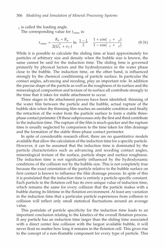
306 Modeling and Simulation of Mineral Processing Systems
L is called the loading angle.The corresponding value for tsmax is:
tR R
U vL
Lsb p
b T
L p
L pmax =
+
2( * + ) ln 1 – 1 + cos( + )
1 – cos( + )(9.31)
While it is possible to calculate the sliding time at least approximately forparticles of arbitrary size and density when the bubble size is known, thesame cannot be said for the induction time. The sliding time is governedprimarily by physical factors and the hydrodynamics in the water phaseclose to the bubble. The induction time, on the other hand, is influencedstrongly by the chemical conditioning of particle surface. In particular thecontact angles, advancing and receding, play an important role. In additionthe precise shape of the particle as well as the roughness of its surface and themineralogical composition and texture of its surface all contribute strongly tothe time that it takes for stable attachment to occur.
Three stages in the attachment process have been identified: thinning ofthe water film between the particle and the bubble, actual rupture of thebubble skin when the thinning film reaches an unstable condition and finallythe retraction of the water from the particle surface to form a stable three-phase contact perimeter. Of these subprocesses only the first and third contributeto the induction time. The rupture of the film is much quicker and the rupturetime is usually neglected by comparison to the time taken for film drainageand the formation of the stable three-phase contact perimeter.
In spite of considerable research effort, there are no quantitative modelsavailable that allow the calculation of the induction time for a specific particle.However, it can be assumed that the induction time is dominated by theparticle characteristics such as advancing and receding contact angles,mineralogical texture of the surface, particle shape and surface roughness.The induction time is not significantly influenced by the hydrodynamicconditions of the collision nor by the bubble size. This is not completely truebecause the exact orientation of the particle relative to the bubble surface onfirst contact is known to influence the film drainage process. In spite of thisit is postulated that the induction time is entirely a particle-specific constant.Each particle in the flotation cell has its own unique value of induction time,which remains the same for every collision that the particle makes with abubble during its lifetime in the flotation environment. At least any variationin the induction time that a particular particle experiences from collision tocollision will reflect only small statistical fluctuations around an averagevalue.
This postulate of particle specificity for the induction time leads to animportant conclusion relating to the kinetics of the overall flotation process.If any particle has an induction time larger than the sliding time associatedwith a direct center line collision with the largest available bubble, it willnever float no matter how long it remains in the flotation cell. This gives riseto the concept of a non-floatable component for every type of particle. This
Flotation 307
behavior is commonly observed during kinetic studies on flotation systemsand has been routinely applied to the analysis of flotation kinetics since atleast the 1950s and probably much earlier than that.
Non-floatable particles will be found in virtually any flotation environmentfrom precisely controlled Hallimond tubes through to large industrial flotationcells. The only exception will be in situations where the particles are conditionedto have very hydrophobic surfaces so that they all have induction times shortby comparison with available sliding times. Under these conditions particlecapture is dominated by the collision process and this is often exploited tomeasure the collision efficiency experimentally.
The collision and sliding phenomena that are described above are illustratedgraphically in the sequence of photographs in Figure 9.2, which show a singlebubble during its sojourn in a fairly typical flotation environment. Thesephotographs show clearly that the particles slide over the front surface of thebubble and accumulate in the lower hemisphere. The close packing of theparticles reflects their ability to form stable particle–particle agglomeratesbecause of their hydrophobic character. The layer of packed particles graduallybuilds up on the bubble and eventually encroaches on the upper hemispherewhere it reduces the sliding time as the load on the bubble increases. Oncethe particle layer crosses the equator of the bubble, the bubble loading startsto impact the rate of transfer of particles to the bubble phase and this must betaken into account when developing models based on the flotation kinetics.
9.3 Distributed rate constant kinetic model forflotation
The kinetic model for flotation is based on Equation 9.3. This equation showsclearly that the rate of transfer of particles of type ij from the pulp phase tothe bubble phase is first order with respect to the concentration of theseparticles in the pulp phase. This observation leads to a simple formulation ofthe kinetic law as
Rate of transfer of particles of type ij = KijCij (9.32)
where
K D d U vGD
E E Eij p pi b Tijv b
bCij Aij Dij = 3
2( + ) ( + ) (1 – )2
3
= 14
1 + ( + ) (1 – )2d
DU v S E E E
pi
bb Tij v Cij Aij Dij (9.33)
= ijSv
and
SGDv
v b
b =
6 m bubble surface/m cell2 3 (9.34)
308 Modeling and Simulation of Mineral Processing Systems
is the total bubble surface area in contact with the pulp phase per unit volumeof the cell. It is easy to see from Equation 9.33 that Kij has units of s–1. Kij is acomplex function of particle size and particles density because of the complexdependence of ECij and EAij on the size of the particles. ij is a mass transfercoefficient for transfer of particles from the pulp to the surface of the bubblesand it can be scaled independently of the bubble surface area. ij has units ofm/s.
Equation 9.33 appears to be a perfectly conventional linear kinetic law butthe Sutherland principle imparts a special character to Kij. A definite fractionof the particles of type ij (i.e. particles characterized by size dpi and mineralogicalgrade gj) have Kij = 0 because tind > tsmax for these particles and therefore EAij= 0. This is the non-floatable fraction for this particle type.
The size of the non-floatable fraction depends on the distribution of inductiontimes across the population of particles that are characterized by size dpi andmineralogical composition g. There is apparently no experimental data fromwhich these distributions can be estimated although experimental techniqueshave been developed for the measurement of induction times. Since theinduction time cannot be negative, it is reasonable to postulate that its valuehas a gamma distribution defined by the probability density function:
f t
tt
ijij
ij ij
ij
ij( ) =
exp –
( )ind
ind–1 ind
(9.35)
which has two parameters ij and ij that vary with particle size and particlecomposition.
The fraction of the particles in class ij that are non-floatable is usuallyspecified in terms of the ultimate recovery, �ij, of particles of this type
�ij = Prob{tind < ts max} (9.36)
where ts max is the longest sliding time available and is given by Equation9.28.
Using Equations 9.35 and 9.36, the ultimate recovery of particles of type ijis given by
�ij
z ij
ij =
( )( )
(9.37)
Where z is the incomplete gamma function and
zts
ij =
max(9.38)
The parameters ij and ij in the distribution of induction times are relateduniquely to the mean and variance of the distribution.
ij t = Variance
Mean = ind
2
ind(9.39)
Flotation 309
ijij
t = Mean = ind
2
2 (9.40)
tind is the average of the induction time distribution and ind2 its variance.
The specific flotation constant for the floatable component of particles oftype ij in given by Equation 9.33 with the appropriate value of the attachmentefficiency EAij.
The attachment efficiency for the floatable fraction of particles of type ij isgiven by
EAij = Prob{ts – tind > 0} (9.41)
Equation 9.41 contains two random variables tind and ts and the indicatedprobability can be evaluated from their respective density functions.
The sliding time ts inherits its randomness from the collision angle cwhich in turn inherits its randomness from the position of the particles relativeto the axis of the bubble motion. c has probability distribution functiongiven by Equation 9.22 and distribution density function:
f c c c( ) = cos (9.42)
ts is related to c by Equation 9.27 and its distribution density function is:
ff
dtd
tc
s
c
sc = ( )
(9.43)
Thus
E f t f t dt dtAij
t t
t s ij s
s s
s = ( ) ( )0 0
ind ind
max
= ( ) ( )0
2f F t dc c ij s c (9.44)
= cos ( )0
2c ij s cF t d
where fij is the distribution density function for the induction time given byEquation 9.35 and Fij is the corresponding distribution function. In practicalapplications the integral in Equation 9.44 must be evaluated numerically butthis is comparatively easy to do.
9.4 Bubble loading during flotationUp to now the discussion of the kinetic model for flotation has been presentedfrom the point of view of the particles. Some additional considerations emerge
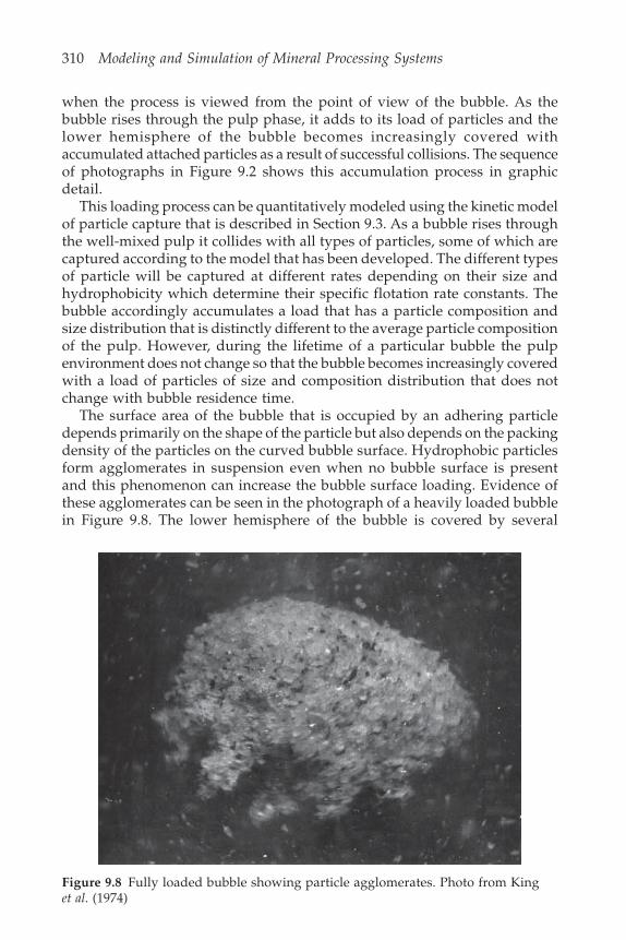
310 Modeling and Simulation of Mineral Processing Systems
when the process is viewed from the point of view of the bubble. As thebubble rises through the pulp phase, it adds to its load of particles and thelower hemisphere of the bubble becomes increasingly covered withaccumulated attached particles as a result of successful collisions. The sequenceof photographs in Figure 9.2 shows this accumulation process in graphicdetail.
This loading process can be quantitatively modeled using the kinetic modelof particle capture that is described in Section 9.3. As a bubble rises throughthe well-mixed pulp it collides with all types of particles, some of which arecaptured according to the model that has been developed. The different typesof particle will be captured at different rates depending on their size andhydrophobicity which determine their specific flotation rate constants. Thebubble accordingly accumulates a load that has a particle composition andsize distribution that is distinctly different to the average particle compositionof the pulp. However, during the lifetime of a particular bubble the pulpenvironment does not change so that the bubble becomes increasingly coveredwith a load of particles of size and composition distribution that does notchange with bubble residence time.
The surface area of the bubble that is occupied by an adhering particledepends primarily on the shape of the particle but also depends on the packingdensity of the particles on the curved bubble surface. Hydrophobic particlesform agglomerates in suspension even when no bubble surface is presentand this phenomenon can increase the bubble surface loading. Evidence ofthese agglomerates can be seen in the photograph of a heavily loaded bubblein Figure 9.8. The lower hemisphere of the bubble is covered by several
Figure 9.8 Fully loaded bubble showing particle agglomerates. Photo from Kinget al. (1974)
Flotation 311
layers of particles where evidently not every particle is in contact with thebubble surface.
A model for bubble loading by particles on its surface can be based on thespecific coverage achieved by each type of particle.
Let ij be the load per unit volume of bubble on a bubble fully loaded withparticles of type ij
ijij b pi pi ij
b
R R R
R =
(1 – )3( + ) + kg/m
20
33 bubble volume (9.45)
ij is the packing voidage for particles of type ij, ij is the density of particlesof type ij and 0 is the load on a very small bubble that is composed largelyof agglomerates of hydrophobic particles.
A fully loaded bubble in a flotation pulp carries a load given by
L V mb ij ij ijmax = (9.46)
where Vb is the volume of the bubble and mij is the mass fraction of particlesof type ij in the bubble load.
L m R R Rij ij ij pi ij b pimax
20 = 4 (1 – ) ( + ) + (9.47)
Lmax can be measured by capturing single completely loaded bubbles andweighing the bubble load. For very small bubbles the maximum load isapproximately independent of the bubble volume and for bubbles that aremuch larger than the particle size, Lmax varies approximately as Vb
2/3 . If theparticles are all of the same size and density
Lmax = a(Rb + Rpi)2 + 0 (9.48)
Some data from captured fully loaded bubbles are given in Figure 9.9.The development of the bubble load L is described by the following
differential equation as the bubble moves through the pulp phase and itsresidence time increases:
6 = maxG L
DdLd
K Cv b
b ij ij ij (9.49)
with Kij given by Equation 9.33 and representing the bubble residencetime.
During the first few seconds of the loading process L < 0.5 and the righthand side of Equation 9.49 is constant and the bubble load increases linearlywith bubble residence time. As the load on the bubble increases, the rate ofloading decreases as a result of two effects. As the solid load carried by thebubble increases, its rise velocity decreases because of its increased mass.Since Kij is proportional to Ub according to Equation 9.33, it decreases as therise velocity decreases. When the load on the bubble exceeds 50%, Kij decreaseswith increase in bubble load because the sliding time, and therefore EAij,
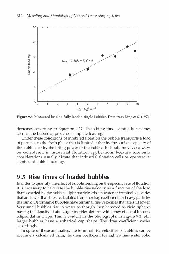
312 Modeling and Simulation of Mineral Processing Systems
decreases according to Equation 9.27. The sliding time eventually becomeszero as the bubble approaches complete loading.
Under these conditions of inhibited flotation the bubble transports a loadof particles to the froth phase that is limited either by the surface capacity ofthe bubbles or by the lifting power of the bubble. It should however alwaysbe considered in industrial flotation applications because economicconsiderations usually dictate that industrial flotation cells be operated atsignificant bubble loadings.
9.5 Rise times of loaded bubblesIn order to quantify the effect of bubble loading on the specific rate of flotationit is necessary to calculate the bubble rise velocity as a function of the loadthat is carried by the bubble. Light particles rise in water at terminal velocitiesthat are lower than those calculated from the drag coefficient for heavy particlesthat sink. Deformable bubbles have terminal rise velocities that are still lower.Very small bubbles rise in water as though they behaved as rigid sphereshaving the density of air. Larger bubbles deform while they rise and becomeellipsoidal in shape. This is evident in the photographs in Figure 9.2. Stilllarger bubbles have a spherical cap shape. The drag coefficient variesaccordingly.
In spite of these anomalies, the terminal rise velocities of bubbles can beaccurately calculated using the drag coefficient for lighter-than-water solid
50
40
30
20
10
00 1 2 3 4 5 6 7 8 9 10
Lmax = 3.5(Rb + Rp)2 + 5
(Rb + Rp)2 mm2
Bub
ble
load
mg
Figure 9.9 Measured load on fully loaded single bubbles. Data from King et al. (1974)
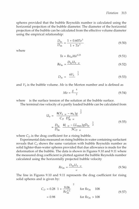
Flotation 313
spheres provided that the bubble Reynolds number is calculated using thehorizontal projection of the bubble diameter. The diameter of the horizontalprojection of the bubble can be calculated from the effective volume diameterusing the empirical relationship:
DD
Ta
Tabe
bh =
1 + 0.601 +
3
3(9.50)
where
Ta = RebeMo0.23 (9.51)
ReD U
bebe b w = (9.52)
DV
beb =
613
(9.53)
and Vb is the bubble volume. Mo is the Morton number and is defined as
Mog
= 4
3 (9.54)
where is the surface tension of the solution at the bubble surface.The terminal rise velocity of a partly loaded bubble can be calculated from
UV m g
C D
DD
LL gDC
bb w b
D bh w
be
bh
w be
D w
= 8( – )
=4( – )
3
2
12
max
12
(9.55)
where CD is the drag coefficient for a rising bubble.Experimental data measured on rising bubbles in water containing surfactant
reveals that Cd shows the same variation with bubble Reynolds number assolid lighter-than-water spheres provided that due allowance is made for thedeformation of the bubble. The data is shown in Figures 9.10 and 9.11 wherethe measured drag coefficient is plotted against the bubble Reynolds numbercalculated using the horizontally projected bubble velocity
ReD U
bhbh b w
w = (9.56)
The line in Figures 9.10 and 9.11 represents the drag coefficient for risingsolid spheres and is given by:
CRe
Re
Re
Dbh
bh
bh
= 0.28 1 + 9.06 for 108
= 0.98 for > 108
1/2
2
(9.57)
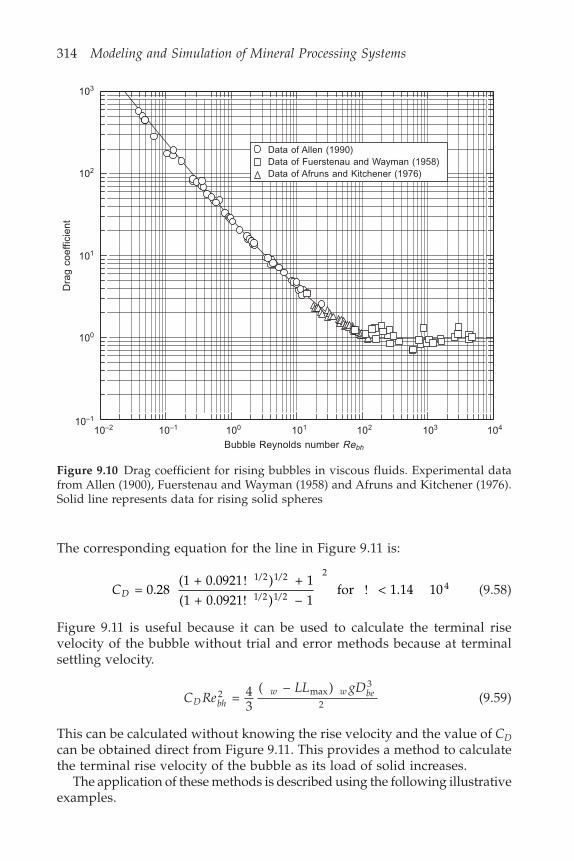
314 Modeling and Simulation of Mineral Processing Systems
The corresponding equation for the line in Figure 9.11 is:
CD = 0.28(1 + 0.0921 ) + 1(1 + 0.0921 ) – 1
for < 1.14 101/2 1/2
1/2 1/2
24!
!! (9.58)
Figure 9.11 is useful because it can be used to calculate the terminal risevelocity of the bubble without trial and error methods because at terminalsettling velocity.
C ReLL gD
D bhw w be2 max
3
2 = 43
( – )(9.59)
This can be calculated without knowing the rise velocity and the value of CDcan be obtained direct from Figure 9.11. This provides a method to calculatethe terminal rise velocity of the bubble as its load of solid increases.
The application of these methods is described using the following illustrativeexamples.
Figure 9.10 Drag coefficient for rising bubbles in viscous fluids. Experimental datafrom Allen (1900), Fuerstenau and Wayman (1958) and Afruns and Kitchener (1976).Solid line represents data for rising solid spheres
103
102
101
100
10–1
10–2 10–1 100 101 102 103 104
Data of Allen (1990)Data of Fuerstenau and Wayman (1958)Data of Afruns and Kitchener (1976)
Bubble Reynolds number Rebh
Dra
g co
effic
ient

Flotation 315
Illustrative example 9.1Calculate the terminal rise velocity of the following bubbles in a dilute aqueoussolution of butanol having surface tension 0.052 N/m. The density of thewater is 999.1 kg/m3, and its viscosity 0.001 kg/ms.
(a) Small bubble of volume effective diameter = 0.5 mm.
! = = 43
22 3
2C RegD
D bhw be
= 43
999.1 9.81 (0.5 10 )(0.001)
2 –3 3
2
= 1.63 103
The value of CD can now be evaluated from Figure 9.11 or Equation 9.58
103
102
101
100
10–1
10–1 100 101 102 105103 104
Data of Allen (1990)Data of Fuerstenau and Wayman (1958)Data of Afruns and Kitchener (1976)
Dra
g co
effic
ient
106 107
Figure 9.11 Drag coefficient for rising bubbles in viscous fluids. Experimental datafrom Allen (1900), Fuerstenau and Wayman (1958) and Afruns and Kitchener (1976).Solid line represents data for rising solid spheres. This coordinate system is mostuseful for the calculation of the terminal rise velocity of bubbles
! = 2C Red bh
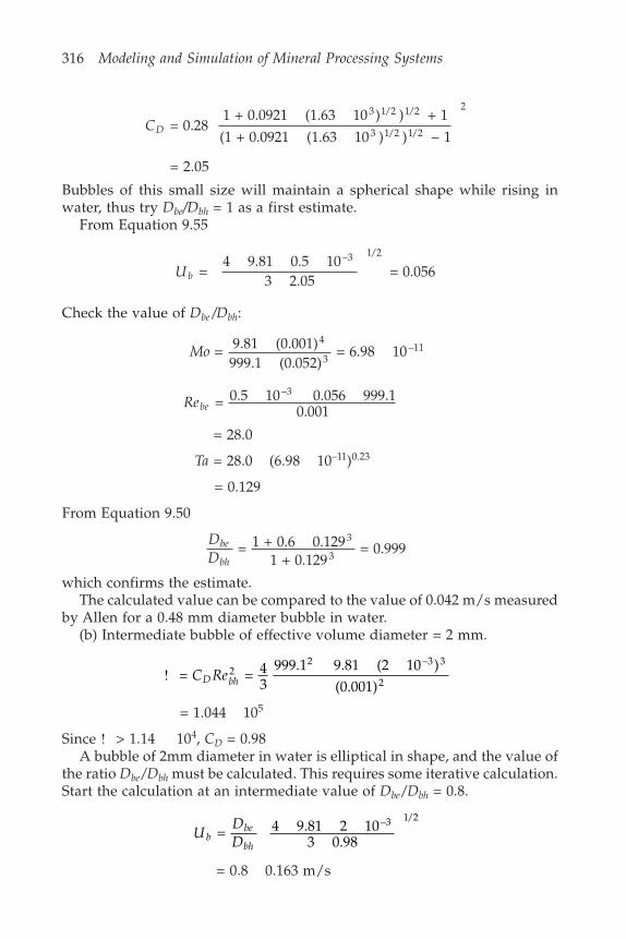
316 Modeling and Simulation of Mineral Processing Systems
CD = 0.281 + 0.0921 (1.63 10 ) ) + 1
(1 + 0.0921 (1.63 10 ) ) – 1
3 1/2 1/2
3 1/2 1/2
2
= 2.05
Bubbles of this small size will maintain a spherical shape while rising inwater, thus try Dbe/Dbh = 1 as a first estimate.
From Equation 9.55
Ub = 4 9.81 0.5 10
3 2.05 = 0.056
–3 1/2
Check the value of Dbe /Dbh:
Mo = 9.81 (0.001)999.1 (0.052)
= 6.98 104
3–11
Rebe = 0.5 10 0.056 999.10.001
–3
= 28.0
Ta = 28.0 (6.98 10–11)0.23
= 0.129
From Equation 9.50
DD
be
bh = 1 + 0.6 0.129
1 + 0.129 = 0.999
3
3
which confirms the estimate.The calculated value can be compared to the value of 0.042 m/s measured
by Allen for a 0.48 mm diameter bubble in water.(b) Intermediate bubble of effective volume diameter = 2 mm.
! = = 43
999.1 9.81 (2 10 )(0.001)
22 –3 3
2C ReD bh
= 1.044 105
Since ! > 1.14 104, CD = 0.98A bubble of 2mm diameter in water is elliptical in shape, and the value of
the ratio Dbe /Dbh must be calculated. This requires some iterative calculation.Start the calculation at an intermediate value of Dbe /Dbh = 0.8.
UDDb
be
bh = 4 9.81 2 10
3 0.98–3 1/2
= 0.8 0.163 m/s

Flotation 317
The diameter ratio must now be refined.
Rebe = 2 10 0.8 0.163 999.10.001
–3
= 261
Ta = 261 (6.98 10–11)0.23
= 1.204
DD
be
bh = 1 + 0.6 1.204
1 + 1.204 = 0.746
3
3
Refining the value of Ub using this value for the diameter ratio gives
DD
be
bh = 0.76
and
Ub = 0.76 0.163 = 0.124 m/s
This answer can be compared to the value of 0.136 m/s measured by Fuerstenauand Wayman (1958) for a 1.97 mm bubble in water.
(c) Large bubble having volume effective diameter = 12 mm.Bubbles as large as this will have a spherical cap shape, and therefore CD =0.98 and the diameter ratio has the limiting value 0.6
Ub = 0.6 4 9.81 12 103 0.98
–3 1/2
= 0.24 m/s
This can be compared with the value 0.236 m/s measured by Fuerstenau andWayman for a bubble having a volume effective diameter of 12.2 mm.
Illustrative example 9.2Calculate the terminal rise velocity of a 0.5 mm diameter air bubble that iscarrying 5 galena particles that may be taken as cubes of side 100 m. Thedensity of galena is 7500 kg/m3.
The specific load carried by the bubble is
5 (100 10 ) 7500
6(0.5 10 )
= 573.0 kg/m–6 3
–3 3
3
! = = 43
(999.1 – 573.0)999.1 9.81 (0.5 10 )(0.001)
2–3 3
2C ReD bh
= 6.96

318 Modeling and Simulation of Mineral Processing Systems
CD = 0.281 + 0.0921 696 ) + 1
1 + 0.0921 696 ) – 1
1/2 1/2
1/2 1/2
2
= 11.21
Ub = 4(999.1 – 573.0)9.81 0.5 10
3 11.21 999.1
–3 1/2
= 0.016 m/s
which is about 13 of the rise velocity of an unloaded bubble.
Illustrative example 9.3Calculate the specific flotation rate constant for 100 m galena particles on0.5 mm diameter bubbles in a continuous flotation cell that is aerated at0.013 m3 air/m3 pulp. The bubble residence time is 5 s. Consider the casewhere the average induction time for the particles is 100 ms. Calculate thefraction of the non-floatable component for these particles. Consider the casewhen the bubble is carrying 5 galena particles ind
2 = 90.
SolutionCalculate the terminal settling velocity of the galena particles, which may beassumed to be cubic in shape. See illustrative example 4.4.
dep
= 6
= 6 10
= 1.241 10 m1/3 –12 1/3
–4∀
= = (1.241 10 )
6 10 = 0.806
2 –4 2
–8
da
e
p
vT = 0.022 m/s
From illustrative example 9.2, the bubble rise velocity = 0.030 m/s.Calculate Ec:
rRRp
p
b = = 0.05
0.25 = 0.2
ReD U
bb b w
w = =
0.5 10 0.030 999.10.001
= 14.9–3
From Equation 9.8
= exp – 4 14.945
0.21.2
0.72#
= 0.901
Flotation 319
Ub* = 0.030 32
(1 – 0.901 + 0.901 0.2) + 12
–34
0.901 0.2 2
= 0.0124
E r rc p p = 3(1 – ) + 32
2
= 3(1 – 0.901)0.2 + 32
0.901 0.22
= 0.114
mp = 5 (100 10–6)3 7500
= 3.75 10–8
= 0.0375 10–6
Vb = 6
(0.5 10 )–3 3
= 6.545 10–11
Assuming the cubic particles pack closely together on the bubble, they occupya total area = 5 10–8 m2. The total surface area of the bubble is (0.5 10–3)2
= 7.85 10–7 m2.
Fractional load on bubble = = 5 107.85 10
= 0.064–8
–7L
Since this is less than half load, tsmax is calculated from Equation 9.28.
pp
b p
RR R
= +
= 5.0 100.25 10 + 5.0 10
–6
3 –6
= 0.167 radians
ts max–3 –6
= 0.25 10 + 50 102(0.0124 + 0.022)
ln1 – cos
2 + 0.167
1 + cos2
+ 0.167
1 + cos(0.1671 – cos(0.167)
= 4.35 10–3 ln [1.40 142.8]
= 0.023 s
EA is evaluated by numerical integration of Equation 9.44.
320 Modeling and Simulation of Mineral Processing Systems
E F t dA c s c = cos ( ) = 0.6360
2ind
The specific rate constant for transfer from pulp to bubble phase can becalculated from Equation 9.33.
∀ = 32
(1 + ) ( + ) 2r U E Eb T C A
= 32
(1 + 0.2) (0.030 + 0.022) 0.114 0.6362
= 8.14 10–3 m/s
KGD
b
b =
= 0.013 50.5 10
8.14 10–3–3 = 1.06 s–1
These calculated rate constants apply only to those particles in the pulp thathave an induction time smaller than tsmax. The remainder make up the non-floatable component. The fraction of pyrite particles that are non-floatable iscalculated from the Equation 9.37.
= Average induction time
Variance of induction time
2
= (100 10 )90 10
–3 2
–3 = 0.111
= 90 10100 10
= 0.9 s–3
–3
zts
= = 0.0230.9
= 0.0255max
Non-floatable fraction = 1 –(0.111)(0.111)
= 0.299z
These calculations can be repeated throughout the range of possible values ofthe parameter tind and for different particle loads on the bubble. The resultsare shown in Figure 9.12. The decrease in flotation rate constant with increasein the particle load is clearly evident in Figure 9.12. While the load is less than50%, both the collision and attachment efficiencies remain constant becausethe colliding particle does not receive any interference from the adheringparticles which are all on the lower hemisphere of the bubble. The decreasein the rate constant is due entirely to the reduction in the bubble rise velocity

Flotation 321
3.0
2.4
1.8
1.2
0.6
0.00.0 0.2 0.4 0.6 0.8 1.0
Particle load on bubble
Spe
cific
flot
atio
n ra
te c
onst
ant s
–1
1.0
0.8
0.6
0.4
0.2
0.00.0 0.2 0.4 0.6 0.8 1.0
Particle load on bubble
Non
-flo
atab
le fr
actio
n
t ind = 10 ms
tind = 50 ms
tind = 100 ms
tind = 200 ms
tind = 500 ms
tind = 500 ms
tind = 200 ms
tind = 100 ms
tind = 50 ms
tind = 10 ms
as the load of particles increases. Once the load exceeds 50%, the attachmentefficiency decreases as the available free bubble surface on the upper hemispherereduces and the rate constant decreases more rapidly. The rate constant reducesto close to zero when the load reaches a mass that the bubble is unable to liftand the number of collisions is reduced to a small number that is governedby the settling velocity of the solid particles in the pulp.
Figure 9.12 Calculated values of the specific flotation rate constant and thecorresponding non-floatable fraction for 100 m galena particles on 0.5 mm diameterbubbles. The parameter is the average of the induction time distribution for the particles
Since there are bubbles in all states of loading in the flotation cell, anaverage bubble loading must be calculated to fix the value of Kij for the pulpvolume as a whole. A method for doing this is described in connection withthe simplified model in Section 9.8.
9.6 Particle detachmentIn the previous sections it has been assumed that if a particle collides withand adheres to a bubble it will enter the froth phase when the carryingbubble breaks through the pulp–froth interface. This is not necessarily sobecause a particle can become detached from a bubble due to the effects ofstresses that are induced by the turbulence in the flotation cell. The detachmentprocess is complex and no comprehensive analysis is available. Two forcesare dominant in causing a particle to become detached from a bubble: theweight of the particle and the inertia of the particle during the acceleration ofthe bubble that is induced by turbulent eddies in the fluid. The distortion ofthe bubble due to the weight of the particle is illustrated in Figure 9.13. Thebubble is distorted and the three-phase contact line is pulled back over theparticle until a position of equilibrium is established or until the bond betweenparticle and bubble is broken. In the ideal situation that is illustrated in

322 Modeling and Simulation of Mineral Processing Systems
Figure 9.13, the separating force Fg is balanced by the vertical component Fcof the surface tension force F . If the separating force exceeds the maximumvalue that Fc can achieve, the particle will be detached. The maximum valueof Fc is obtained as follows:
Fc = 2 Rp sin sin∃ (9.60)
Bubble Fc F
Rb
Rp
Particle
Fg
%
Figure 9.13 Distortion of a bubble due to weight of an attached particle. Adaptedfrom Drzymala (1994)
This must be maximized subject to the condition that + ∃ = where is thecontact angle. Setting the derivative of Fc equal to zero shows that Fc ismaximized when
∃ = = 2
(9.61)
F Rc pmax2 = 2 sin
2 (9.62)
The largest particle that can attach to the bubble in a quiescent pulp is givenby

Flotation 323
6( – ) = sin
2max3
max2d g dp s w p (9.63)
dgp
s wmax
12
= 6
( – )sin
2(9.64)
The additional forces caused by turbulence can detach a smaller particle andan approximate analysis by Woodburn et al. (1971) leads to the followingmodel for the detachment efficiency.
Ed
dDp
p =
max
1.5
(9.65)
9.7 The froth phase
9.7.1 Motion of the frothThe kinetic models for the collection of solid particles in the pulp are notadequate to describe the overall behavior of the flotation cell because thefroth on the top of the cell exerts a strong influence on the kinetic behavior ofthe flotation system. The processes that take place in the froth phase arecomplex and they ultimately determine whether a particle that is capturedby a bubble in the pulp phase will be recovered in the concentrate streamfrom the flotation cell. Two aspects of froth behavior must be considered: themotion of the froth from the surface of the pulp towards the upper surface ofthe froth and the concentrate overflow weir and the processes that occurwithin the froth while it is flowing. These processes include bubble bursting,particle detachment and drainage of water and solids from the froth. It isuseful to consider the motion of the froth first and then superimpose theinternal subprocesses on the basic flow pattern.
Bubbles, carrying their loads of attached particles, leave the pulp phaseand pass into the froth phase at the pulp–froth boundary at the top of thepulp. The bubbles do not burst immediately and they congregate togetherand float on the surface of the pulp. The bubbles are pushed upward steadilyby the arrival of new bubbles from the pulp phase. Provided that the bubblesare not too large, they retain their spherical shape as they pass from the pulpinto the lower layer of the froth phase. They tend to arrange themselves in ahexagonal close-packed arrangement with the intervening spaces betweenthe bubbles filled with liquid that is carried upward with the bubble from thepulp phase. This interstitial liquid entrains significant quantities of particulatematerial from the pulp and the entrained material can include significantquantities of hydrophilic non-floating particles. The composition of theentrained solids is determined primarily by the composition of the solid thatis suspended in topmost regions of the pulp phase.
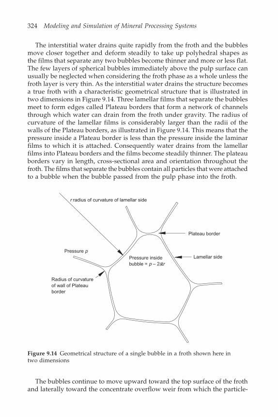
324 Modeling and Simulation of Mineral Processing Systems
The interstitial water drains quite rapidly from the froth and the bubblesmove closer together and deform steadily to take up polyhedral shapes asthe films that separate any two bubbles become thinner and more or less flat.The few layers of spherical bubbles immediately above the pulp surface canusually be neglected when considering the froth phase as a whole unless thefroth layer is very thin. As the interstitial water drains the structure becomesa true froth with a characteristic geometrical structure that is illustrated intwo dimensions in Figure 9.14. Three lamellar films that separate the bubblesmeet to form edges called Plateau borders that form a network of channelsthrough which water can drain from the froth under gravity. The radius ofcurvature of the lamellar films is considerably larger than the radii of thewalls of the Plateau borders, as illustrated in Figure 9.14. This means that thepressure inside a Plateau border is less than the pressure inside the laminarfilms to which it is attached. Consequently water drains from the lamellarfilms into Plateau borders and the films become steadily thinner. The plateauborders vary in length, cross-sectional area and orientation throughout thefroth. The films that separate the bubbles contain all particles that were attachedto a bubble when the bubble passed from the pulp phase into the froth.
r radius of curvature of lamellar side
Pressure p
Radius of curvatureof wall of Plateauborder
Plateau border
Lamellar sidePressure insidebubble = p – 2&/r
Figure 9.14 Geometrical structure of a single bubble in a froth shown here intwo dimensions
The bubbles continue to move upward toward the top surface of the frothand laterally toward the concentrate overflow weir from which the particle-
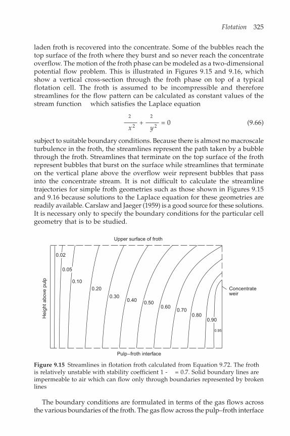
Flotation 325
Hei
ght a
bove
pul
p
0.02
0.05
0.100.20
0.300.40 0.50
0.600.70
0.800.90
0.95
Pulp–froth interface
Concentrateweir
Upper surface of froth
laden froth is recovered into the concentrate. Some of the bubbles reach thetop surface of the froth where they burst and so never reach the concentrateoverflow. The motion of the froth phase can be modeled as a two-dimensionalpotential flow problem. This is illustrated in Figures 9.15 and 9.16, whichshow a vertical cross-section through the froth phase on top of a typicalflotation cell. The froth is assumed to be incompressible and thereforestreamlines for the flow pattern can be calculated as constant values of thestream function which satisfies the Laplace equation
2
2
2
2 + = 0x y
(9.66)
subject to suitable boundary conditions. Because there is almost no macroscaleturbulence in the froth, the streamlines represent the path taken by a bubblethrough the froth. Streamlines that terminate on the top surface of the frothrepresent bubbles that burst on the surface while streamlines that terminateon the vertical plane above the overflow weir represent bubbles that passinto the concentrate stream. It is not difficult to calculate the streamlinetrajectories for simple froth geometries such as those shown in Figures 9.15and 9.16 because solutions to the Laplace equation for these geometries arereadily available. Carslaw and Jaeger (1959) is a good source for these solutions.It is necessary only to specify the boundary conditions for the particular cellgeometry that is to be studied.
Figure 9.15 Streamlines in flotation froth calculated from Equation 9.72. The frothis relatively unstable with stability coefficient 1 - = 0.7. Solid boundary lines areimpermeable to air which can flow only through boundaries represented by brokenlines
The boundary conditions are formulated in terms of the gas flows acrossthe various boundaries of the froth. The gas flow across the pulp–froth interface

326 Modeling and Simulation of Mineral Processing Systems
Upper surface of froth
Hei
ght a
bove
pul
p
Pulp–froth interface
Concentrateweir
0.02
0.05
0.100.20
0.30
0.400.50
0.600.70
0.80
0.90
0.95
is related to the aeration rate in the flotation cell G m3/s. Consider a flotationcell with a rectangular cross-section and a side-to-side dimension w metersand a front-to-back dimension b meters. The superficial gas velocity throughthe pulp–froth interface is G/wb and the linear aeration rate is G/w per unitlength of interface. The total gas flow through the interface that is boundedby the back wall of the cell and an imaginary line a distance x from the backwall is Gx/b. Thus, if the value of the stream function against the back wallis given the reference value 0, the value of the stream function at a distancex from the back wall is = (Gx/b). The stream function can be normalized as:
= G
(9.67)
and also obviously satisfies Equation 9.66. The dimensions of the froth arenormalized with respect to the cell dimension b.
x xb
yyb
=
= (9.68)
On the pulp–froth interface the boundary value for the stream function isgiven by = x .
Similarly the stream function is zero along the entire back wall because noair passes through that plane. No gas passes through the front wall beneaththe overflow weir. An important feature of the pattern of streamlines in thefroth is the fractional split of the gas flow between that contained in the
Figure 9.16 Streamlines in flotation froth calculated from Equation 9.72. The froth isrelatively stable with stability coefficient 1 – = 0.3. Solid boundary lines areimpermeable to air which can flow only through boundaries represented by brokenlines
Flotation 327
concentrate froth and that which leaves the froth through the top surfacewhere bubbles burst and release gas. If a fraction 1 – of the froth passesover the weir, the streamline that passes through the top right hand corner ofthe froth is associated with the stream function with normalized value because this streamline separates the recovered froth from the froth thatterminates its life by bursting on the top surface. Thus the boundary conditionalong the top surface of the froth is
= x (9.69)
and along the front wall
= 1 for 0 < y Wh (9.70)
and
= 1 – (1 – )––
for < < y WhH Wh
Wh y H (9.71)
where H represents the total height of the froth layer and Wh represents theheight of the weir above the pulp–froth interface.
The parameter is determined largely by the stability of the froth. Stablefroths tend to rise higher above the pulp thus forcing more froth over theweir into the concentrate. Unstable froth tends to break more easily andconsequently more gas leaves the froth through the top surface. Lower valuesof represent more stable froths. Obviously the mobility of the froth alsoaffects the value of parameter since greater mobility of the froth phase willallow more to be recovered over the weir.
Carslaw and Jaeger provide a convenient steady state solution to Equation9.66 in a rectangular region with three sides having = 0 and an arbitraryfunction along the fourth side. The solution to the present problem can beobtained by superimposing three separate solutions each with the appropriateboundary function specified for the pulp–froth interface, the top surface ofthe froth or the front wall and concentrate overflow.
The general solution has the form
(x , y ) = 1(x , y ) + 2(1 – x , H – y ) + 3(y , 1 – x ) (9.72)
where
i n nix y a n x
n H yn H
n y( , ) = sin 1 – exp(–2 ( – ))
1 – exp(–2 ) exp(– )
=1( )
∋ (9.73)
represents the solution for boundary i and the coefficients ani( ) for each solution
are given by
ann
n(1) = – 2 (–1) (pulp–froth interface)
ann
(2) = 2
(upper surface of froth) (9.74)
328 Modeling and Simulation of Mineral Processing Systems
an n Wh
n Whnn(3) = 2 1 – (–1) + 1 –
(1 – )sin( ) (front edge)
The contours for constant values of (the streamlines) calculated from Equation9.72 are illustrated in Figures 9.15 and 9.16. These figures give a visual pictureof the flow of the froth.
9.7.2 Dynamic processes in the froth phaseAs individual bubbles in the froth move upward towards the free surfaceand laterally toward the overflow weir, a number of dynamic processes occur.The most obvious of these is the coarsening of the froth structure due torupture of the lamellar films between the bubbles. A rupture of this kindgives rise to a sudden increase in the bubble volume and the froth structurebecomes increasingly coarse. This phenomenon is easily observable on anyflotation cell and there are a number of studies underway aimed at diagnosingthe behavior of the froth from the size of bubbles in the top layer which canbe measured fairly easily by image analysis techniques.
The rupturing of a film in the froth leads to the partial detachment of thehydrophobic particles that were present in the film before rupture. The waterand particles contained in the ruptured lamellar film are transferred to theplateau borders that are connected to the film. It is reasonable to suppose thatsome of the particles will, however, remain attached at the air–water interfaceand will simply move to a neighboring lamellar film. Particles that have ahigh hydrophobicity (high contact angle) will have a greater tendency toremain attached while particles with lower hydrophobicity will tend to transferto the Plateau borders. This is the origin of the upgrading that can occur inthe froth, a phenomenon that has been observed in experiments.
The water in the Plateau borders together with its load of suspendedsolids drains under gravity through the network of Plateau borders so thefroth becomes steadily denuded of both water and particles as it moves towardthe overflow weir.
Hydrophilic particles that entered the froth by entrainment are unlikely tobecome attached to bubbles in the froth and they are free to drain from thefroth with the water. Particles also settle relative to the water because of theirgreater density and this adds to the downward flux of particles in the Plateauborders.
Particles that are entrained in the water in the lamellar films that separatethe bubbles do not drain from the lamellar films to the Plateau borders becausethey are hindered by other particles that are attached to the bubble surfaces.This restriction was first suggested by Gaudin who provided a sketch toillustrate the idea.
The rate of breakage of lamellar films is governed in a complex fashion bythe surface tension of the fluid, the concentration and type of surfactants, thethickness of the film, the presence of particles, particularly those having highcontact angles, the differential pressure across the film and the size of the

Flotation 329
bubble, and therefore the area of the film. Dippenaar (1982) has demonstratedthat hydrophobic particles with high contact angles lead to fairly rapid filmrupture but there is also evidence that hydrophobic particles with lowercontact angles have a stabilizing effect on the froth. This can sometimes beobserved in flotation plants where the froths produced in cleaner cells areoften more stable than those produced in rougher or scavenger cells.
The dynamic behavior of the froth and its evolution with time is governedby three rate processes: the rate of drainage of water from the lamellar filminto the Plateau borders, the rate of breakage of the lamellar films, and therate of drainage of water and suspended solids from the Plateau borders. Inaddition, the compositions of the particle populations in the lamellar filmsand the Plateau borders at any point in the froth phase are governed by thedifferential rate of detachment of the different types of particle from thelamellar films into the Plateau borders.
These individual rate processes are difficult to observe and study in thelaboratory so that almost no reliable information is currently available onappropriate model structures that can be used for their description inquantitative terms. It is however useful to formulate a simple model for eachprocess and to superimpose these on the model of the froth motion that isdescribed in Section 9.7.1. This leads to an overall kinetic model for theflotation process that captures the elements of the all important subprocessesthat occur in the froth and which is capable of calibration against operatingdata. This model for the froth phase can be combined with the kinetic modelsfor the pulp phase to generate a viable model structure that can be used forsimulation of operating flotation cells and flotation plants.
9.7.3 Rate of breakage of lamellar filmsThe rate of breakage of the lamellar films that separate bubbles in the froth isa complex process that depends on many factors. The two internal propertiesof the froth that are most directly affected by the rupturing of the lamellarfilms are the surface area per unit volume of froth and the amount andcomposition of the solids that remain attached to the bubble surfaces. Theamount of water and solid and the composition of the solid in the Plateauborders is also determined by the film breakage process because each ruptureevent adds both water and, selectively, solid particles to the Plateau borders.
The rate at which lamellar films break varies throughout the froth layerbut the factors that determine the rate of breakage are not well enoughunderstood at the present time to attempt anything but the simplest simulationof this subprocess and its effect on the performance of the flotation cell.Accordingly a simple model for the breakage of lamellar films is used here.A method is now developed to calculate amount and composition of thesolid concentrate and the amount of water that is recovered over the weir.
The method of solution is based on the observation that individual bubblespass through the froth entirely on a single streamline. Thus the dynamicchanges that occur during the time that a bubble is in the froth can be evaluated
330 Modeling and Simulation of Mineral Processing Systems
by integration along a streamline. This can be illustrated by calculating bubblesurface area per unit volume of froth from the time that a bubble enters thefroth until it leaves in the concentrate or bursts on the surface of the froth. LetSF represent bubble surface area per unit volume of froth. A differential balanceon the surface area in the froth gives
uSx
uSy
RxF
yF
B + = – (9.75)
where ux and uy are the local components of the froth motion and RB is therate of breakage of lamellar films per unit volume of froth. The incompressibilityof the froth requires
ux
uy
x y + = 0 (9.76)
The solution to Equation 9.75 can be generated by integrating along a streamlinesince all streamlines are characteristic lines for this equation. The localcomponents of the velocity vector can be obtained by differentiation of thestream function.
uw y
Gwb y
Gwb
u U ux x G x = 1 = = = (9.77)
and uw x
Gwb x
Gwb
u U uy y G y = – 1 = – = = (9.78)
where UG = (G/wb) is the superficial gas velocity across the pulp–froth interface.Along a streamline
dSdy
Ru
F B
y = – (9.79)
which is easy to integrate numerically starting at SF = (6/Db) at y = 0. Db is thediameter of the bubble as it leaves the pulp phase. It is convenient to normalizeSF with respect to the surface area per unit volume of a single sphericalbubble as it emerges from the pulp phase and RB with respect to the surfacearea production rate in the flotation cell 6G/Db
S SD
F Fb =
6(9.80)
R RD wb
GB Bb = 6
2(9.81)
Then Equation 9.79 becomes
dSdy
Ru
F B
y = – (9.82)
with S yF = 1 at = 0.
Flotation 331
Each bubble burst alters the amount of solid that is attached to the bubblesurfaces that bound the lamellar films because there is a strong tendency forthe attached solid to become detached and to enter the water in the Plateauborders as suspended solid. Not all of the adhering solid will become detachedand some will remain attached at the air–water interface and will slide alongthe surface and join the attached load on a neighboring lamellar film. Thisphenomenon is described by a solid attachment coefficient ij which is thefraction of particles of type ij that remain attached during a bursting event.
ij depends strongly on the size and hydrophobicity of the particle. Highlyhydrophobic particles have a greater tendency to remain attached and this isthe primary mechanism by which the grade of mineral increases in the frothas the froth moves up from the pulp surface. This phenomenon has beenobserved in practice and is sometimes exploited to improve the grade of theconcentrate in industrial flotation cells. The composition of the solid attachedto bubble surfaces is governed by the equation
uS
xu
Sy
RxF ij
yF ij
ij ij B + = –(1 – ) (9.83)
where ij is the amount of solid of type ij attached per unit area of bubblesurface. ij is the fraction of type ij that remains attached during the ruptureof a single lamellar film. The streamlines are characteristics for Equation 9.83and along a streamline
dSdy
Ru
F ij ij ij B
y = –
(1 – )(9.84)
which must be integrated from the initial condition ij = mijLLmax at y = 0.LLmax is the load carried by the bubbles when they leave the pulp phase andmij is the mass fraction of particles of type ij in the bubble load. ij is normalizedby
ijij
ijm LL =
max(9.85)
and Equation 9.84 is normalized
ddy
RS u
ijij
ij B
F y = (9.86)
SF ij and can be calculated along a characteristic streamline using Equations9.82 and 9.86 provided that a model for bubble bursting rate can be formulated.The rate at which laminar films rupture is assumed here to be constant.
The residence time of any bubble in the froth is obtained by integratingalong a streamline
ddy uy
= 1 (9.87)
332 Modeling and Simulation of Mineral Processing Systems
where is the bubble residence time normalized with respect to the superficialvelocity of the gas.
= Ub
G (9.88)
Equations 9.82 and 9.86 can be integrated simultaneously to give explicitexpressions for SF ij and throughout the froth in terms of the residence timeas a parameter.
S RF B = 1 – (9.89)
ij F BS Rij ij = ( ) = (1 – )– – (9.90)
These expressions are necessary for calculating the conditions in the networkof Plateau borders throughout the froth as descibed in Section 9.7.4.
9.7.4 Froth drainage through plateau bordersFlow of slurry in the network of Plateau borders varies throughout the froth.The rate at which water and solids drain through the network is larger at thebottom of the froth because of the accumulated water and solids due tobreakage of lamellar films as the froth flows toward the surface or theconcentrate weir. The water and solids that drain from the lamellar films andwhich leaves the films because of the breakage mechanism that is describedin Section 9.7.3 causes a steady increase in the flow through the Plateauborders which increase in cross-sectional area to accommodate the additionalflow. The slurry that drains through the Plateau borders is driven by gravityand consequently moves relative to the moving froth.
The path that any element of draining slurry takes through the froth canbe calculated from the streamlines established for the froth and therefore forthe network of Plateau borders which moves integrally with the froth. Thevelocity at which the slurry drains relative to the network can be approximatedby assuming laminar flow under gravity in the Plateau borders. A shortsegment of a channel within the network of Plateau borders might appear asshown in Figure 9.17. In a channel inclined at angle to the vertical theaverage velocity relative to the channel wall is:
Vg DH( ) =
cos32
2
(9.91)
where DH is the hydraulic diameter of the channel. The Plateau borders areassumed to have no preferred orientation so that is uniformly distributedin the interval [0, /2]. The average draining velocity is
Vg D
dH = 23
cos 0
/2 2
2
=16
2g DH (9.92)
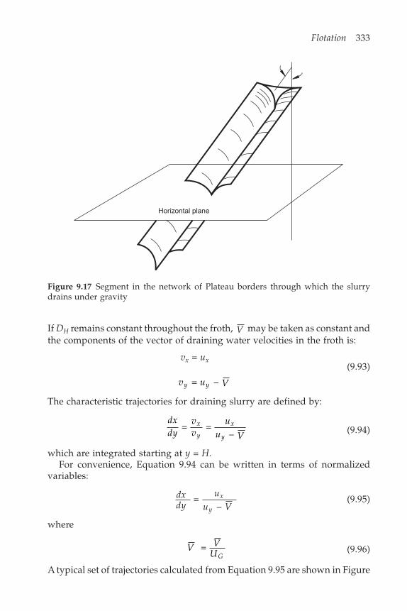
Flotation 333
If DH remains constant throughout the froth, V may be taken as constant andthe components of the vector of draining water velocities in the froth is:
vx = ux(9.93)
v u Vy y = –
The characteristic trajectories for draining slurry are defined by:
dxdy
vv
uu V
x
y
x
y = =
– (9.94)
which are integrated starting at y = H.For convenience, Equation 9.94 can be written in terms of normalized
variables:
dxdy
uu V
x
y =
–(9.95)
where
V VUG
= (9.96)
A typical set of trajectories calculated from Equation 9.95 are shown in Figure
Horizontal plane
Figure 9.17 Segment in the network of Plateau borders through which the slurrydrains under gravity
334 Modeling and Simulation of Mineral Processing Systems
9.16. Trajectories that pass over the concentrate weir represent water andsolids that are recovered by entrainment. Those trajectories that end on thepulp–froth interface represent slurry that is returned from the froth to thepulp phase.
The quantity of slurry that drains through the network of Plateau bordersincreases steadily from the top of the froth because the bursting bubblescontinually add water to the drainage channels, which become increasinglylarger in cross-section to accommodate the increase in the rate of drainage. If represents the volume of the Plateau borders per unit volume of froth, the
differential volume balance for the draining slurry is
ux
u V yRx y B( + ( – ) = 1
2 (9.97)
where ( is the average thickness of the lamellar films in the froth. Equation9.97 must be solved with boundary conditions specified along the top surfaceof the froth, which reflect the release of slurry due to the bursting of thebubbles on that surface. All lamellar films break that are associated with thegas that escapes through the top surface of the froth and the slurry producedenters the Plateau borders and starts to drain down the network of channels.Any wash water that is added to the top surface of the froth also adds to theflow at the upper surface.
V S UF G( = 12
+ wash water rate at y = H(9.98)
( = 3 + wash water rateS
V VF
The drainage trajectories shown in Figure 9.18 are characteristic lines for thesolution of Equation 9.97. Along any trajectory
ddy
Ru V
B
y
( = 1
2 – (9.99)
In terms of normalized variables
ddy
R
u VB
y
( =
3
– (9.100)
where ( = (( /Db).A differential balance for the concentration Cij of solids of type ij in the
slurry in the Plateau borders is
uCx
u V vCy
Rxij
y Tijij
ij B ij + ( – – ) = (1 – ) (9.101)
where vTij is the terminal settling velocity in the narrow channels of particlesof type ij. Boundary conditions are:

Flotation 335R
ear
wal
l of f
lota
tion
cell
Upper surface of froth
Pulp–froth interface
Concentrateweir
C y Hijij
= 2
at = ( (9.102)
Characteristic lines for this equation can be calculated by integrating:
dxdy
u
u VvU
x
yTij
G
= – –
(9.103)
These lines have the same general shape as the drainage characteristics butare somewhat steeper, becoming almost vertical throughout most of the frothfor particles that settle rapidly.
Along these characteristic lines
d Cdy
R
u V vij ij B ij
y Tij =
(1 – )
– –(9.104)
In terms of normalized variables:
d Cdy
R
u VvU
ij ij B ij
yTij
G
= (1 – )
– –(9.105)
with
CC D
m LLijij b
ij =
6 max(9.106)
Figure 9.18 Drainage trajectories for slurry in the network of Plateau borders
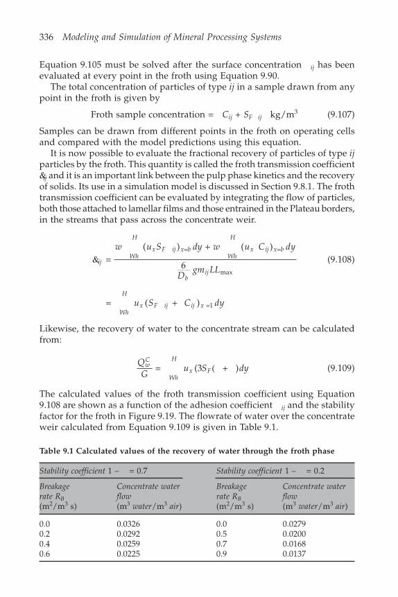
336 Modeling and Simulation of Mineral Processing Systems
Table 9.1 Calculated values of the recovery of water through the froth phase
Stability coefficient 1 – = 0.7 Stability coefficient 1 – = 0.2
Breakage Concentrate water Breakage Concentrate waterrate RB flow rate RB flow(m2/m3 s) (m3 water/m3 air) (m2/m3 s) (m3 water/m3 air)
0.0 0.0326 0.0 0.02790.2 0.0292 0.5 0.02000.4 0.0259 0.7 0.01680.6 0.0225 0.9 0.0137
Equation 9.105 must be solved after the surface concentration ij has beenevaluated at every point in the froth using Equation 9.90.
The total concentration of particles of type ij in a sample drawn from anypoint in the froth is given by
Froth sample concentration = Cij + SF ij kg/m3 (9.107)
Samples can be drawn from different points in the froth on operating cellsand compared with the model predictions using this equation.
It is now possible to evaluate the fractional recovery of particles of type ijparticles by the froth. This quantity is called the froth transmission coefficient&ij and it is an important link between the pulp phase kinetics and the recoveryof solids. Its use in a simulation model is discussed in Section 9.8.1. The frothtransmission coefficient can be evaluated by integrating the flow of particles,both those attached to lamellar films and those entrained in the Plateau borders,in the streams that pass across the concentrate weir.
&ijWh
H
x F ij x bWh
H
x ij x b
bij
w u S dy w u C dy
Dgm LL
= ( ) + )
6
= =
max
((9.108)
= ( + ) =1Wh
H
x F ij ij xu S C dy
Likewise, the recovery of water to the concentrate stream can be calculatedfrom:
QG
u S dywC
Wh
H
x F = (3 + )( (9.109)
The calculated values of the froth transmission coefficient using Equation9.108 are shown as a function of the adhesion coefficient ij and the stabilityfactor for the froth in Figure 9.19. The flowrate of water over the concentrateweir calculated from Equation 9.109 is given in Table 9.1.
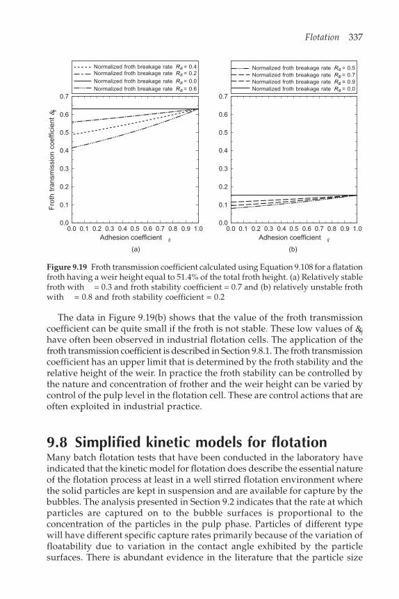
Flotation 337
The data in Figure 9.19(b) shows that the value of the froth transmissioncoefficient can be quite small if the froth is not stable. These low values of &ijhave often been observed in industrial flotation cells. The application of thefroth transmission coefficient is described in Section 9.8.1. The froth transmissioncoefficient has an upper limit that is determined by the froth stability and therelative height of the weir. In practice the froth stability can be controlled bythe nature and concentration of frother and the weir height can be varied bycontrol of the pulp level in the flotation cell. These are control actions that areoften exploited in industrial practice.
9.8 Simplified kinetic models for flotationMany batch flotation tests that have been conducted in the laboratory haveindicated that the kinetic model for flotation does describe the essential natureof the flotation process at least in a well stirred flotation environment wherethe solid particles are kept in suspension and are available for capture by thebubbles. The analysis presented in Section 9.2 indicates that the rate at whichparticles are captured on to the bubble surfaces is proportional to theconcentration of the particles in the pulp phase. Particles of different typewill have different specific capture rates primarily because of the variation offloatability due to variation in the contact angle exhibited by the particlesurfaces. There is abundant evidence in the literature that the particle size
0.7
0.6
0.5
0.4
0.3
0.2
0.1
0.00.0 0.1 0.2 0.3 0.4 0.5 0.6 0.7 0.8 0.9 1.0
0.7
0.6
0.5
0.4
0.3
0.2
0.1
0.00.0 0.1 0.2 0.3 0.4 0.5 0.6 0.7 0.8 0.9 1.0
Adhesion coefficient ij Adhesion coefficient ij
Normalized froth breakage rate RB = 0.4Normalized froth breakage rate RB = 0.2Normalized froth breakage rate RB = 0.0Normalized froth breakage rate RB = 0.6
Normalized froth breakage rate RB = 0.5Normalized froth breakage rate RB = 0.7Normalized froth breakage rate RB = 0.9Normalized froth breakage rate RB = 0.0
(a) (b)
Fro
th t
rans
mis
sion
coe
ffici
ent
& ij
Figure 9.19 Froth transmission coefficient calculated using Equation 9.108 for a flatationfroth having a weir height equal to 51.4% of the total froth height. (a) Relatively stablefroth with = 0.3 and froth stability coefficient = 0.7 and (b) relatively unstable frothwith = 0.8 and froth stability coefficient = 0.2
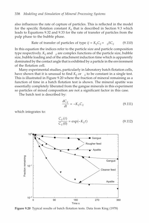
338 Modeling and Simulation of Mineral Processing Systems
also influences the rate of capture of particles. This is reflected in the modelfor the specific flotation constant Kij that is described in Section 9.3 whichleads to Equations 9.32 and 9.33 for the rate of transfer of particles from thepulp phase to the bubble phase.
Rate of transfer of particles of type ij = KijCij = ijSCij (9.110)
In this equation the indices refer to the particle size and particle compositiontype respectively. Kij and ij are complex functions of the particle size, bubblesize, bubble loading and of the attachment induction time which is apparentlydominated by the contact angle that is exhibited by a particle in the environmentof the flotation cell.
Many experimental studies, particularly in laboratory batch flotation cells,have shown that it is unusual to find Kij or ij to be constant in a single test.This is illustrated in Figure 9.20 where the fraction of mineral remaining as afunction of time in a batch flotation test is shown. The mineral apatite wasessentially completely liberated from the gangue minerals in this experimentso particles of mixed composition are not a significant factor in this case.
The batch test is described by:
dCdt
K Cij
ij ij = – (9.111)
which integrates to:
C tC
K tij
ijij
( )(0)
= exp(– ) (9.112)
Figure 9.20 Typical results of batch flotation tests. Data from King (1978)
100
10–1
10–2
0 90 180 270 360
Gangue
Rougher feed
Apatite
Gangue
Cleaner feed
Apatite
Time s
Frac
tion
rem
aini
ng
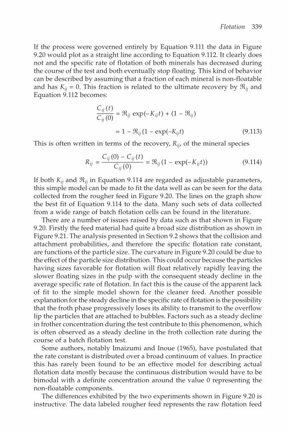
Flotation 339
If the process were governed entirely by Equation 9.111 the data in Figure9.20 would plot as a straight line according to Equation 9.112. It clearly doesnot and the specific rate of flotation of both minerals has decreased duringthe course of the test and both eventually stop floating. This kind of behaviorcan be described by assuming that a fraction of each mineral is non-floatableand has Kij = 0. This fraction is related to the ultimate recovery by �ij andEquation 9.112 becomes:
C tC
K tij
ijij ij ij
( )(0)
= exp(– ) + (1 – )� �
= 1 – �ij (1 – exp(–Kijt) (9.113)
This is often written in terms of the recovery, Rij, of the mineral species
R
C C tC
K tijij ij
ijij ij =
(0) – ( ) = (1 – exp(– )
( )0� ) (9.114)
If both Kij and �ij in Equation 9.114 are regarded as adjustable parameters,this simple model can be made to fit the data well as can be seen for the datacollected from the rougher feed in Figure 9.20. The lines on the graph showthe best fit of Equation 9.114 to the data. Many such sets of data collectedfrom a wide range of batch flotation cells can be found in the literature.
There are a number of issues raised by data such as that shown in Figure9.20. Firstly the feed material had quite a broad size distribution as shown inFigure 9.21. The analysis presented in Section 9.2 shows that the collision andattachment probabilities, and therefore the specific flotation rate constant,are functions of the particle size. The curvature in Figure 9.20 could be due tothe effect of the particle size distribution. This could occur because the particleshaving sizes favorable for flotation will float relatively rapidly leaving theslower floating sizes in the pulp with the consequent steady decline in theaverage specific rate of flotation. In fact this is the cause of the apparent lackof fit to the simple model shown for the cleaner feed. Another possibleexplanation for the steady decline in the specific rate of flotation is the possibilitythat the froth phase progressively loses its ability to transmit to the overflowlip the particles that are attached to bubbles. Factors such as a steady declinein frother concentration during the test contribute to this phenomenon, whichis often observed as a steady decline in the froth collection rate during thecourse of a batch flotation test.
Some authors, notably Imaizumi and Inoue (1965), have postulated thatthe rate constant is distributed over a broad continuum of values. In practicethis has rarely been found to be an effective model for describing actualflotation data mostly because the continuous distribution would have to bebimodal with a definite concentration around the value 0 representing thenon-floatable components.
The differences exhibited by the two experiments shown in Figure 9.20 isinstructive. The data labeled rougher feed represents the raw flotation feed
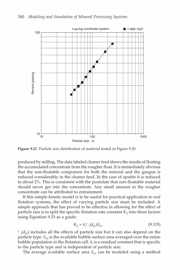
340 Modeling and Simulation of Mineral Processing Systems
100
1010 100 1000
Per
cent
pas
sing
Log-log coordinate system
Particle size m
1 NIM 1847
produced by milling. The data labeled cleaner feed shows the results of floatingthe accumulated concentrate from the rougher float. It is immediately obviousthat the non-floatable component for both the mineral and the gangue isreduced considerably in the cleaner feed. In the case of apatite it is reducedto about 2%. This is consistent with the postulate that non-floatable materialshould never get into the concentrate. Any small amount in the rougherconcentrate can be attributed to entrainment.
If this simple kinetic model is to be useful for practical application to realflotation systems, the effect of varying particle size must be included. Asimple approach that has proved to be effective in allowing for the effect ofparticle size is to split the specific flotation rate constant Kij into three factorsusing Equation 9.33 as a guide:
Kij = kj! j(dpi)Sav (9.115)
! j(dpi) includes all the effects of particle size but it can also depend on theparticle type. Sav is the available bubble surface area averaged over the entirebubble population in the flotation cell. kj is a residual constant that is specificto the particle type and is independent of particle size.
The average available surface area Sav can be modeled using a method
Figure 9.21 Particle size distribution of material tested in Figure 9.20
Flotation 341
proposed by Pogorely (1962) who noted that the rate at which the availablesurface area on a bubble decreases can be modeled by Equation 9.49:
V A dSd
MAS k d p MASkc j j j pi ij! = ( ) = (9.116)
where M is the mass of solids in the cell and pij is the fraction of the solids inthe cell that is in composition class j and size class i. Vc is the volume of theflotation cell and A is the bubble surface area per unit volume.
The available surface area after the bubble has been in the cell for a time is obtained by integration of Equation 9.116
S MV
k d p
M kV
c j j j pi ij
c
= exp – ( )
= exp –
! (9.117)
The average available area in the cell is obtained by averaging S over theinterval from 0 to b where b is the time that a bubble spends in the cell.
S S SdS VM k
M kVav v
v c
b
b
c
b
= = 1 – exp –0
(9.118)
9.8.1 Application to flotation cells in complexflowsheets
The rate of transfer of particles of type ij to the froth phase in a perfectlymixed flotation cell is
Rate of transfer = kj! j(dpi)SavMpij kg/s (9.119)
A material balance for particles of type ij is:
W p W p W pFijF C
ijC T
ijT = +
= ( ) + & !ij j j pi av ijT T
ijTk d S Mp W p (9.120)
where &ij is the froth transmission coefficient for particles of type ij.
W pW p
k d S MW
TijT
FijF
ij j j pi av T
= 1 + ( )& !
(9.121)
The residence time of the solids in the cell is based on the flowrate of tailings
T TM
W = (9.122)
which is usually approximated as
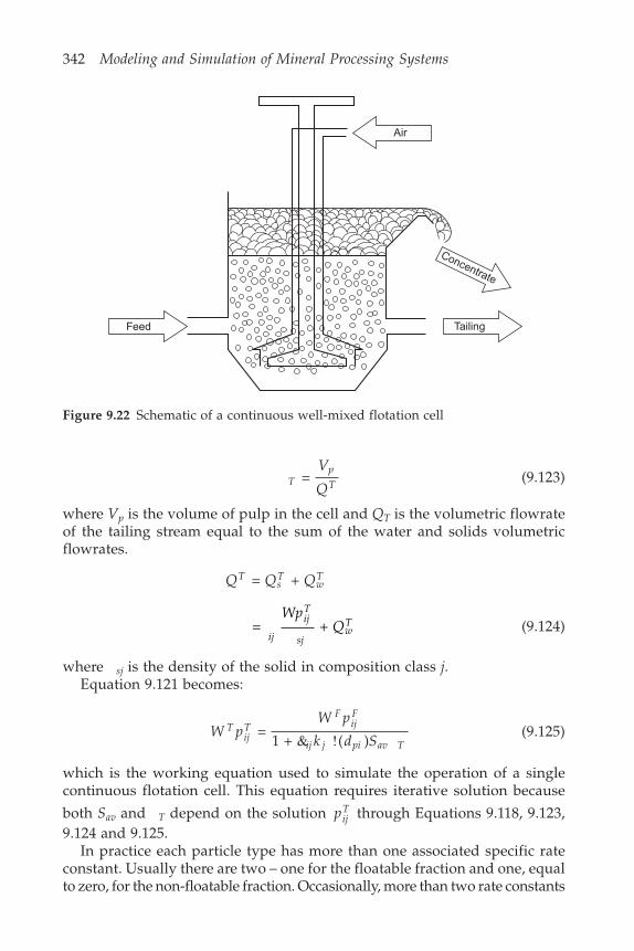
342 Modeling and Simulation of Mineral Processing Systems
TpT
V
Q = (9.123)
where Vp is the volume of pulp in the cell and QT is the volumetric flowrateof the tailing stream equal to the sum of the water and solids volumetricflowrates.
Q Q QTsT
wT = +
= + ij
ijT
sjwT
WpQ (9.124)
where sj is the density of the solid in composition class j.Equation 9.121 becomes:
W pW p
k d ST
ijT
FijF
ij j pi av T =
1 + ( )& ! (9.125)
which is the working equation used to simulate the operation of a singlecontinuous flotation cell. This equation requires iterative solution because
both Sav and T depend on the solution pijT through Equations 9.118, 9.123,
9.124 and 9.125.In practice each particle type has more than one associated specific rate
constant. Usually there are two – one for the floatable fraction and one, equalto zero, for the non-floatable fraction. Occasionally, more than two rate constants
Air
Concentrate
TailingFeed
Figure 9.22 Schematic of a continuous well-mixed flotation cell
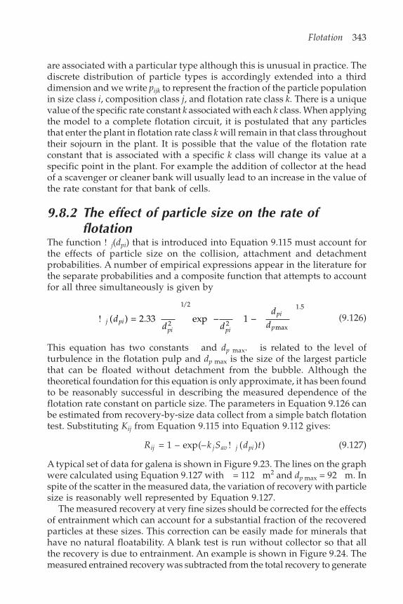
Flotation 343
are associated with a particular type although this is unusual in practice. Thediscrete distribution of particle types is accordingly extended into a thirddimension and we write pijk to represent the fraction of the particle populationin size class i, composition class j, and flotation rate class k. There is a uniquevalue of the specific rate constant k associated with each k class. When applyingthe model to a complete flotation circuit, it is postulated that any particlesthat enter the plant in flotation rate class k will remain in that class throughouttheir sojourn in the plant. It is possible that the value of the flotation rateconstant that is associated with a specific k class will change its value at aspecific point in the plant. For example the addition of collector at the headof a scavenger or cleaner bank will usually lead to an increase in the value ofthe rate constant for that bank of cells.
9.8.2 The effect of particle size on the rate offlotation
The function ! j(dpi) that is introduced into Equation 9.115 must account forthe effects of particle size on the collision, attachment and detachmentprobabilities. A number of empirical expressions appear in the literature forthe separate probabilities and a composite function that attempts to accountfor all three simultaneously is given by
! j pipi pi
pi
pd
d d
dd
( ) = 2.33 exp – 1 –2
1/2
2 max
1.5
(9.126)
This equation has two constants and dp max. is related to the level ofturbulence in the flotation pulp and dp max is the size of the largest particlethat can be floated without detachment from the bubble. Although thetheoretical foundation for this equation is only approximate, it has been foundto be reasonably successful in describing the measured dependence of theflotation rate constant on particle size. The parameters in Equation 9.126 canbe estimated from recovery-by-size data collect from a simple batch flotationtest. Substituting Kij from Equation 9.115 into Equation 9.112 gives:
R k S d tij j av j pi = 1 – exp(– ( ) )! (9.127)
A typical set of data for galena is shown in Figure 9.23. The lines on the graphwere calculated using Equation 9.127 with = 112 m2 and dp max = 92 m. Inspite of the scatter in the measured data, the variation of recovery with particlesize is reasonably well represented by Equation 9.127.
The measured recovery at very fine sizes should be corrected for the effectsof entrainment which can account for a substantial fraction of the recoveredparticles at these sizes. This correction can be easily made for minerals thathave no natural floatability. A blank test is run without collector so that allthe recovery is due to entrainment. An example is shown in Figure 9.24. Themeasured entrained recovery was subtracted from the total recovery to generate
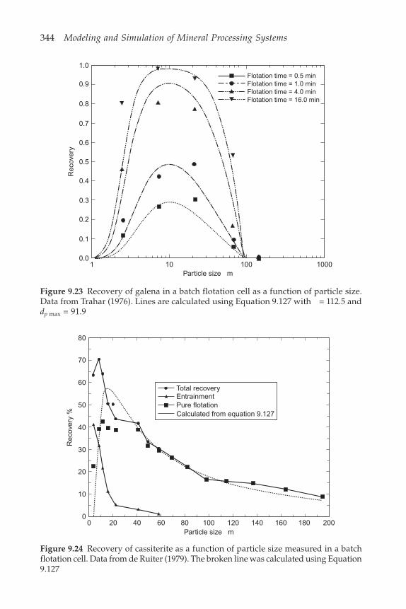
344 Modeling and Simulation of Mineral Processing Systems
Calculated from equation 9.127Pure flotationEntrainmentTotal recovery
80
70
60
50
40
30
20
10
00 20 40 60 80 100 120 140 160 180 200
Particle size m
Rec
over
y %
Figure 9.23 Recovery of galena in a batch flotation cell as a function of particle size.Data from Trahar (1976). Lines are calculated using Equation 9.127 with = 112.5 anddp max = 91.9
Figure 9.24 Recovery of cassiterite as a function of particle size measured in a batchflotation cell. Data from de Ruiter (1979). The broken line was calculated using Equation9.127
1.0
0.9
0.8
0.7
0.6
0.5
0.4
0.3
0.2
0.1
0.0
Rec
over
y
Particle size m1 10 100 1000
Flotation time = 0.5 minFlotation time = 1.0 minFlotation time = 4.0 minFlotation time = 16.0 min
Flotation 345
the true flotation recovery, which is represented by square symbols in thefigure. The true flotation recovery is compared to that calculated from Equation9.127 in the figure. The function ! j(dpi) given by Equation 9.126 with = 130
m2 and dp max = 400 m fits the data well.The parameter in Equation 9.126 is comparatively easy to estimate because
it is related directly to the particle size, dpm at which the recovery is a maximumthrough the equation
= 0.5 2dpm (9.128)
The constant 2.33 in Equation 9.126 normalizes the function so that ! j(dpm) =1.0.
9.8.3 The water balance in an operating flotation cellThe water balance across the flotation cell can be established in a number ofways. The rate of water transfer by bubbles into the froth phase together witha model for froth breakage and drainage is the most reliable model for thispurpose but the model described in Section 9.7 has not yet been developed tothe stage where the parameters can be related for prediction purposes to thethermodynamic properties of the flotation environment. However the stabilitycoefficient 1 – , the froth breakage rate RB and the lamellar film thickness (can be estimated from measurements of the water recovery rate at differentfroth heights. Two alternative methods have been found to be useful in practice:the total solids content of either the concentrate or tailings stream can bespecified.
If the solid content of the concentrate, sC, is specified the calculation of thewater balance is straightforward once Equation 9.125 has been solved. Thevolumetric flowrate of water in the concentrate is
Q ss
W pwC
C
wC ijk
CijkC = 1 – (9.129)
where w is the density of the water. From Equation 9.119:
Q ss
k d S W pwC
C
wC ijk
ij j j pi avT T
pT
ijk = 1 – ( )& ! (9.130)
The water flow in the tailing stream is obtained by difference:
Q Q QwT
wF
wC = – (9.131)
If the solid content, sT, of the tailing stream is specified:
Q ss
W pwT
T
wT ijk
TijkT = 1 – (9.132)
and the water flowrate in the concentrate stream is obtained by difference:
Q Q QwC
wF
wT = – (9.133)
346 Modeling and Simulation of Mineral Processing Systems
9.9 Symbols used in this chapterb Distance from front to back of flotation cell, m.Cij Concentration of particles of type ij in the pulp or in the slurry
entrained in the froth, kg/m3.CD Drag coefficient of a rising bubble.Dbe Volume equivalent bubble diameter, m.Dbh Horizontal projection of bubble diameter, m.dpi Particle size in class i, m.dp max Largest particle that can remain attached to a bubble, m.EAij Attachment efficiency for particles of type ij.ECij Collision efficiency for particles of type ij.EDij Detachment efficiency for particles of type ij.� Function that defines the effect of the radial coordinate on the stream-
line around a rising bubble.F c Distribution of particle collision angles.f c Distribution density for particle collision angles.Fij(tind) Distribution of induction times for particles of type ij.fij(tind) Distribution density for induction times for particles of type ij.G Aeration rate in a flotation cell, m3/s.Gv Specific aeration rate in flotation cell per unit volume of cell, s–1.gj Particle grade in grade class j.Kij Specific flotation rate constant for particles of type ij, s–1.L Fraction of bubble surface that is covered by adhering particles.Lmax Load carried by completely covered bubble.Qs Volumetric flowrate of solid, m3/s.Qw Volumetric flowrate of water, m3/s.r Radial coordinate, m.
r rRb
rpRR
p
bRb Radius of bubble, m.RB Bubble bursting rate in the froth.Rp Radius of particle, m.Ro Distance from collision centerline far in front of bubble, m.Roij Ro for particle of type ij having a grazing trajectory, m.Reb Bubble Reynolds number.�ij Ultimate recovery of particles of type ij.Sav Average available bubble surface area per unit volume of cell, m–1.SF Bubble surface area per unit volume of froth, m–1.Sv Surface area of bubble per unit volume of cell, m–1.tind Induction time, s.ts Sliding time, s.tind Average of the induction time distribution, s.u Velocity vector, m/s.

Flotation 347
Ub Rise velocity of bubble, m/s.UG Superficial velocity of gas through the pulp–froth interface, m/s.v Velocity vector, m/s.vTij Terminal settling velocity of particles of type ij, m/s.
V Average velocity of draining slurry relative to the froth, m/s.W Mass flowrate of solid, kg/s.Wh Weir height, m.x Normalized horizontal coordinate in the froth, x/b.y Normalized vertical coordinate in the froth, y/b.
Parameter for froth stabilityij Parameter for distribution of induction time for particles of type ij.ij Parameter for distribution of induction time for particles of type ij.
&ij Froth transmission coefficient.ij Concentration of particles of type ij attached to bubble surface in
the froth, kg/m2.( Thickness of lamellar film in froth, m.
ij Packing density for particles of type ij on bubble surface, kg/m3.Polar coordinate.
c Collision angle.L Loading angle.p Angle subtended by particle radius when particle touches the bubble
surface.T Residence time of pulp in flotation cell, s.
Specific flotation rate constant, m/s.w Viscosity of water, Pa s.w Density of water, kg/m3.
Variance of induction time distribution, s2.ij Fraction of particles of type ij that remain attached to bubble surface
during a bubble burst event in the froth.Residence time in the froth measured along a froth streamline, s.
! Dimensionless number C ReD bh2 .
! (dp) Function to describe the variation of flotation rate constant withparticle size.Normalized stream function.Stream function.
BibliographyThe fundamental basis of the collision model for flotation kinetics is due toSutherland (1948) and is discussed in detail in Sutherland and Wark (1955).This model has been widely discussed in the literature and many researchershave contributed to its development. Some of the key ideas are developed inFlint and Howarth (1971), Reay and Ratcliffe (1973) and Yoon and Luttrell(1989) and the work of these authors forms the basis of the model for collisionefficiency that is presented here. Many of the hydrodynamic considerations
348 Modeling and Simulation of Mineral Processing Systems
of bubble motion are discussed in Clift et al. (1978). Schulze (1983) has presenteda comprehensive analysis of many aspects of the model.
The model for the rise velocity of bubbles is based on the analysis ofKaramanev and Nikolov (1992) and Karamanev (1994). Data on measuredbubble rise velocities is given by Allen (1900), Fuerstenau and Wayman (1958)and Afruns and Kitchener (1976).
Tomlinson and Fleming (1965) investigated experimentally the effect ofbubble loading on the rate of flotation and described its effects. Measureddata on bubble loading is given by King et al. (1974) and Bradshaw andO’Connor (1996).
The distributed kinetic constant model has been widely discussed andused because laboratory batch experiments can almost invariably be describedusing the concept. The first formal statement that mineral particles showedthe peculiar behavior of possessing a non-floatable component appears to bedue to Morris (1952).
The effect of particle size on the flotation recovery is reviewed by Traharand Warren (1976). The model for particle detachment was based on thepresentation of Drzymala (1994).
Questions relating to the conditioning of the surfaces of the common typesof minerals that are treated by flotation are discussed in King (1982). Somequantitative results are presented but the information is largely qualitativeand therefore not directly applicable to model calculations and simulation.
The potential flow model for the froth phase is due to Moys (1978, 1984).Moys (1989) and Cutting (1989) have summarized measurements that havebeen made by taking samples from the froth of operating flotation cells. Themodel of the froth behavior presented here is based on Murphy et al. (1996),Neethling and Cilliers (1999) and Neethling et al. (2000) who have investigatedthe behavior of froths using experimental and simulation techniques. Theirmethods produce models of the behavior of the froth phase that are significantlymore realistic than the simple model that is used here.
The discrete distributed flotation model originated with Zaidenberg et al.in 1964. The application of this model to the simulation of flotation plants isbased on King (1973, 1975) and Sutherland (1977).
ReferencesAfruns, J.P. and Kitchener, J.A. (1976) The absolute rate of capture of single particles
by single bubbles. Flotation. Gaudin Memorial Volume (M.C. Fuerstenau, ed.).SME, pp. 625–637.
Allen, H.S. (1900) The motion of a sphere in a viscous fluid. Philosophical Magazine,Vol. 50, pp. 323–338.
Bradshaw, D.J. and O’Connor, C.T. (1996) Measurement of the sub-process of bubbleloading in flotation. Minerals Engineering, Vol. 9, pp. 443–448.
Carslaw, H.S. and Jaeger, J.C. (1959) Conduction of Heat in Solids. Oxford UniversityPress, Oxford.
Clift, R., Grace, J.R. and Weber, M.E. (1978) Bubbles, Drops and Particles. AcademicPress.

Flotation 349
Cutting, G.W. (1989) Effect of froth structure and mobility on plant performance.Mineral Processing and Extractive Metallurgy Review, Vol. 5, pp. 169–201.
de Ruiter, M.A. (1979) Particle size effects in the flotation of cassiterite. MSc. ThesisUniversity of the Witwatersrand, Johannesburg.
Dippenaar, A. (1982) The destabilization of froths by solids. International Journal ofMineral Processing, Vol. 9, pp. 1–22.
Drzymala, J. (1994) Characterization of materials by Hallimond tube flotation. Part 2:Maximum size of floating particles and contact angle. Intl Jnl Mineral Processing,Vol. 42, pp. 153–168.
Flint, L.R. and Howarth, W.J. (1971) The collision efficiency of small particles withspherical air bubbles. Chemical Engineering Science, Vol. 26, pp. 115–168.
Fuerstenau, D.W. and Wayman, C.H. (1958) Effect of chemical reagents on the motionof single air bubbles in water. Trans. AIME, Vol. 211, pp. 694–699.
Imaizumi, T. and Inuoe, T. (1965) Kinetic considerations of froth flotation. Proc. 6th
Intl. Mineral Processing Congress (A. Roberts, ed.), Pergamon Press, Oxford.Karamanev, D.G. (1994) Rise of gas bubbles in quiescent liquids. AIChE Journal, Vol.
40, pp. 1418–1421.Karamanev, D.G. and Nikolov, L.N. (1992) Free rising spheres do not obey Newton’s
Law for free settling. AIChE Journal, Vol. 38, pp. 1843–1846.King, R.P. (1973) Model for the design and control of flotation plants. Applications of
Computer Methods in the Mineral Industry (M.D.G. Salamon and F.H. Lancaster, eds).S. Afr. Inst. Min. Metall. Johannesburg, pp. 341–350.
King, R.P. (1975) Simulation of flotation plants. Trans. AIME, Vol. 258, pp. 286–293.King, R.P. (1978) A pilot-plant investigation of a kinetic model for flotation. Jnl South
African Inst. Min. Metall., Vol. 78, pp. 325–338.King, R.P. (ed.) (1982) Principles of Flotation. S. Afr. Inst. Min. Metall. Johannesburg.King, R.P., Hatton, T.A. and Hulbert, D.G. (1974) Bubble loading during flotation.
Trans. Instn Min. Metall., Vol. C, pp. C112–C115.Morris, T.M. (1952) Measurement and Evaluation of the rate of flotation as a function
of particle size. Trans. AIME, Vol. 193, pp. 794–797.Moys, M.H. (1978) A study of a plug flow model for flotation froth behavior. Intl Jnl
Mineral Processing, Vol. 5, pp. 21–38.Moys, M.H. (1984) Residence time distribution and mass transport in the froth phase
of the flotation process. Intl Jnl Mineral Processing, Vol. 13, pp. 117–142.Moys, M.H. (1989) Mass transport in flotation froths. Mineral Processing and Extractive
Metallurgy Review, Vol. 5, pp. 203–228.Murphy, D.G., Zimmerman, W. and Woodburn, E.T. (1996) Kinematic model of bubble
motion in a flotation froth. Powder Technology, Vol. 87, pp. 3–12.Neethling, S.J. and Cilliers, J.J. (1999) A visual kinematic model of flowing foams
incorporating coalescence. Powder Technology, Vol. 101, pp. 249–256.Neethling, S.J., Cilliers, J.J. and Woodburn, E.T. (2000) Prediction of the water distribution
in a flowing foam. Chem. Engng Science, Vol. 55, pp. 4021–4028.Neethling, S.J. and Cilliers, J.J. (2000) A model for free solids motion in froths. Private
communication.Pogorely, A.D. (1962) Limits of the use of the kinetic equation proposed by K F Beloglazov.
Izv. Vuz. Tsvetnaya Metaurgia, No. 1, pp. 33–40. Available in English as NIM-TR-158from Mintek. Randburg, S. Africa.
Reay, D. and Ratcliffe, G.A. (1973) Removal of fine particles from water by dispersedair flotation: effect of bubble size and particle size on collision efficiency. CanadianJournal of Chemical Engineering, Vol. 51, pp. 178–185.
Schulze, H.J. (1993) Physico-chemical Elementary Processes in Flotation. Elsevier, Amsterdam.
350 Modeling and Simulation of Mineral Processing Systems
Sutherland, D.N. (1977) An appreciation of galena concentration using a steady-stateflotation model. Intl Jnl Mineral Processing, Vol. 4, pp. 149–162.
Sutherland, K.L. (1948) Physical chemistry of flotation XI. Kinetics of the flotationprocess. Jnl Physical Chemistry, Vol. 52, pp. 394–425.
Sutherland, K.L. and Wark, I.W. (1955) Principles of Flotation. Australasian Instituteof Mining and Metallurgy. Melbourne.
Tomlinson, H.S. and Fleming, M.G. (1965) Flotation rate studies. Proc. 6th InternationalMineral Processing Congress (A. Roberts, ed.). Pergamon Press.
Trahar W.J. (1976) The selective flotation of galena from sphalerite with special referenceto the effects of particle size. Intl Jnl Mineral Processing, Vol. 3, pp. 151–166.
Trahar, W.J. and Warren, L.J. (1976) The floatability of very fine particles – A review.Intl Jnl Mineral Processing, Vol. 3, pp. 103–131.
Woodburn, E.T., King, R.P. and Colborn, R.P. (1971) The effect of particle size distributionon the performance of a phosphate flotation process. Metallurgical Transactions, Vol.2, pp. 3163–3174.
Yoon, R.H. and Luttrell, G.H. (1989) The effect of bubble size on fine particle flotation.Mineral Processing and Extractive Metallurgy Review, Vol. 5, pp. 101–122.
Zaidenberg, I. Sh., Lisovskii, D.I. and Burovoi, I.A. (1964) One approach to theconstruction of a mathematical model for flotation processes. Soviet Journal of Non-ferrous Metals, English translation, Vol. 5, pp. 26–32.
10Simulation of ore dressingplants
10.1 The nature of simulationMany references appear in the literature to computer simulation as a techniquefor design and analysis of mineral processing operations. It has been afashionable field of research since the 1960s and a great deal of good workhas been done to make simulation into a viable and practical tool. Simulationis any procedure that can be used to model a process without actually runningit. There are several ways in which a simulation can be achieved, but by farthe most effective is by digital computer. The computer is programmed tomimic the behavior of the actual plant and can provide a description of whatthe plant will do and how it will perform under a variety of circumstances.This is a useful thing to do because a simulation can expose many aspects ofplant performance without the inconvenience of operating the plant itselfunder experimental conditions. Although a good computer simulation canprovide information about the behavior and performance of a mineralprocessing plant, it must be used with circumspection and care.
Simulation of a complex engineering system is only possible once a detailedunderstanding of each component of the system has been achieved andsimulation provides the engineer with a tool for the prediction of systembehavior even if the system does not exist in reality. However the simulatorpredictions can only be as good as the basic understanding of the componentparts. The modeling techniques that are described in earlier chapters haveintrinsic interest in their own right in that they attempt to build a quantitativepicture of the operating behavior of the equipment in terms of the underlyingphysical and chemical principles that govern their operation. These modelsprovide a focus for research efforts that are aimed at the development of amore complete and accurate understanding of the detailed mechanisms andprocesses that underlie the behavior of the unit operations. Improvedunderstanding at this level contributes to the technical evolution of processequipment and to the development of new and better unit designs. The focusof this book has been directed towards an additional goal in that the modelshave been developed specifically to provide the building blocks for use in aprocess plant simulator. The models have all been developed with this particularapplication in mind. To be useful and effective in a simulator the modelsmust all fit seamlessly together so that the simulator can function in theintended way. Different models for the same unit operation must also be

352 Modeling and Simulation of Mineral Processing Systems
interchangeable to facilitate their comparison under comparable operatingconditions. The computer is an essential component of simulation for tworeasons: in most systems of interest to the mineral processing engineer, theindividual unit operations are so complex that they can be usefully describedin mathematical terms only if these can be translated into computer code; inaddition the systems of interest reveal complex interactions andinterconnections among the individual units that must be accurately accountedfor. In many cases these complex interactions cannot be described adequatelyby purely mathematical methods and the ability of the computer to transferinformation from one program model to another is exploited effectively tosimulate the transfer of actual material, information or energy in a real system.Purely mathematical formulations of complex systems are effective only whenthe systems are linear in the mathematical sense. Then the full power oflinear and matrix algebra can be brought to bear on the problem. Regrettablymost systems of real interest are rarely linear and it is necessary to use theheuristic capabilities of the computer to take the place of purely mathematicaldescriptions.
An ore dressing plant simulator is a set of computer programs that providesa detailed numerical description of the operation of an ore dressing plant.The simulator must be provided with an accurate description of the ore thatis to be processed, a description of the flowsheet that defines the process andan accurate description of the operating behavior of each unit operation thatis included in the flowsheet. The simulator uses these ingredients to providea description of the operating plant. The detailed description of the ore willinclude information on its physical and mineralogical characteristics and amethod to provide this information is described later. The flowsheet is thefamiliar graphical representation of the location of the unit operations in theplant together with the network of pipes and conveyors that transmit materialbetween the units. The description of the operating behavior of the unitoperations is based on the models that have been developed in earlier chaptersfor the individual equipment types. The simulator links together the modeledbehavior of each of the unit operations and synthesizes the overall performanceof the plant.
Four fundamental concepts underlie the construction of an ore dressingplant simulator.
Ore dressing plants are collections of unit operations connected by processflow streams that transmit material from one unit to the next. The flow ofmaterials is directed by the flowsheet structure.Each unit operation processes its own feed materials and will separate itor transform it in accordance with the specific objective of the unit.The behavior of the plant as a whole depends on the operatingcharacteristics of each of the unit operations as well as on the nature ofthe material that is processed in the plant.A simulator reduces the actual plant operations, as defined by the flowsheet
Simulation of ore dressing plants 353
structure and the behavior of the units, to a sequence of logical mathematicalfunctions. The simulator can then mimic the real plant performance.
These basic concepts are independent of the precise nature of any particularplant that must be simulated and they lead to the development of simulationsoftware that can be used for all possible plant configurations. The availabilityof such general purpose software makes computer simulation a useful practicaltool in everyday engineering. It is a difficult task to write the necessarycomputer code to simulate a complex ore dressing plant. Most engineershave neither the time, inclination nor skill to do so and it would not be costeffective to write the code for each application. The cost in man hours togenerate the code and debug it so that it can run reliably would be enormous.Computerization of any complex engineering systems is a highly specializedtask and this is true also in mineral processing and such activities should beattempted only by specialists. The simulation system that is included on thecompact disc that is included in this book is identified by the name MODSIM.This simulator was developed as a result of the success that was achievedwith a flotation plant simulator that was developed as part of the researchprogram of Mintek’s Chemical Engineering Research Group in the Departmentof Chemical Engineering of the University of Natal, Durban, South Africa(King, 1972). It was the successful application of this flotation plant simulatorto industrial flotation plants (King, Pugh and Langely, 1973) that demonstratedthe potential for simulation techniques and that led to the development ofMODSIM as a simulator for ore-dressing plants of arbitrary configurationand complexity and which contained any of the operations that are associatedwith ore dressing.
The simulation engine in MODSIM was developed as a Ph.D project byM.A. Ford (1979) who wrote the Fortran code for the loop finding, circuitdecomposition and sequential calculation algorithms. This code still formsthe core of MODSIM and it has required only minor modifications to keep itcompatible with modern compilers and other requirements for codemaintenance. This long run of successful computation provides MODSIMwith a stable computational core that can be relied on to perform well evenin the face of the extraordinary wide variety of plant configurations that canbe simulated. The models for the unit operations are independent of theinner core of the simulator and these evolve continually in response to researchendeavors. Consequently new models are frequently added to MODSIM andolder models are improved whenever a new development warrants a change.This evolutionary process will continue well into the future.
The graphics user interface has evolved continually as new software systemsand computing platforms have become available. The original version of theinterface was presented at the 13th CMMI Conference in Johannesburg in1982. Although MODSIM was developed originally for use on large mainframecomputers, the preferred platform is now the ubiquitous desktop PC. Theuser interface is built to modern software engineering standards and it providesan intuitive environment that is designed to make the simulator easy andconvenient to use.
354 Modeling and Simulation of Mineral Processing Systems
Several general-purpose simulators for ore dressing plants are now availableand of these MODSIM offers the greatest versatility to the user to modify andadapt the models of the unit operations that are used by the simulator. Thestandard models that are provided in the package rely on the methods thatare described in this book. MODSIM is particularly strong in the modeling ofmineral liberation phenomena. The underlying theme for the models that areused in MODSIM is the population balance method, which has beenemphasized throughout this book. This methodology is ideally suited to theneeds of a plant simulator because the method enables each type of particleto be tracked as the material that is processed passes through the plant. It isa natural framework within which the models for the unit operations arecast. The structure of MODSIM reflects its basis in the population balancemethod and the user should feel comfortable with this approach after readingthe contents of Chapter 2.
In order for a general-purpose simulator to yield useful information on theactual process to be simulated, it must have access to three important classesof information. These are defined in general terms as follows:
The structure of the flowsheet – what unit operations are included andhow they are connected.The nature of the material to be processed – its mineralogical compositionand structure, the size distribution and the amount that must be processed.The operating characteristics of each unit in the flowsheet. This requiresthe full description of the unit operations (the unit models) and aspecification of the unit parameters that define the operating characteristicsof the individual units.
MODSIM has been used primarily as an academic tool to enhance theeducational experience of students of mineral processing. It appears to havebeen successful since students regularly comment on the improved insightsthat they achieve when they can try out the models, either in single units orin combinations with other units. Many of the operating characteristics of theunit operations that are discussed in the classroom can be easily demonstratedusing the simulator. The modular open-ended structure of MODSIM makesit easy to add new models to the simulator, although this is not possible withthe student version that is included with this book. Professors and lecturerscan obtain the academic version of MODSIM, which is full-featured and doespermit the introduction of new models. The method that is used to write thenecessary code and add the models is fully documented in the user manualincluded on the compact disc.
10.2 Use of the simulatorA good simulator is a useful tool to the process plant engineer. Essentially thesimulator can demonstrate, at least approximately, what a plant will do underany particular operating conditions. It can do so cheaply and without any

Simulation of ore dressing plants 355
real risk to the production rate of an operating plant or it can do so before aplant has been built and it does so in the engineer’s office.
(a) Design studies:At the design stage a good simulator can be used to:
Help the design engineer to find the best flowsheet.Ensure that design specifications will be met under all requiredoperating conditions.Choose the most suitable unit operations to be included in theplant.Size the units correctly and so eliminate wasteful over-design andavoid the catastrophe of under-design.Optimize the plant operation by achieving best economiccombinations of grade and recovery.Identify potential production bottlenecks.Provide comparative assessment of competing manufacturers’equipment.Define the performance guarantees that should be met by suppliers.Find out what will happen if performance guarantees are not met.
(b) Operating plant performance:A good simulator can be used to assist in the operation of a runningplant in ways such as the following:
Optimum performance of the plant can be approached.The plant can be tuned to suit variations in feed quality andflowrate.Plant bottlenecks can be found and appropriate steps taken toeliminate them.Performance changes can be investigated by asking ‘what if’questions.Operations that are not properly understood can be identifiedand appropriate research effort undertaken to remedy such asituation.
Simulation can be seductive and the user of this technique must be skepticaland vigilant. A simulator can be effective only if it gives a reliable and validdescription of plant operations. Generally this means that before simulationcan be used the models that are contemplated must be calibrated againstoperating data that are representative of the conditions that apply to theactual plant operation.
10.3 The flowsheet structureA plant flowsheet consists of a number of unit operations connected togetherby process flow streams. Material enters the plant and passes successivelythrough the process units in accordance with the flowsheet structure, sometimesrecycling on itself until finally it leaves the plant in one or other product

356 Modeling and Simulation of Mineral Processing Systems
stream. The material in a flow stream is processed by each unit in order tochange the nature of the material or to separate it into its constituent parts.The number of different types of unit operation encountered in ore dressingplants is comparatively limited and these can be classified into three generictypes.
10.3.1 The ore dressing unit operationsThere are only three basic types of ore dressing unit operations:
separation units that separate solid particles without changing theircharacteristics, for example flotation and gravity separation;transformation units that alter the characteristics of the solid particles,for example crushing and grinding operations; andunits that separate solid and liquid constituents.
It is remarkable that the entire repertoire of ore dressing unit operations canbe classified by such a simple scheme and this simplicity is exploited effectivelyin the simulator.
A further characteristic of the unit models is the flow stream connectionsthat are possible. Separation units will always produce at least two productstreams, a concentrate and a tailing, or an underflow and an overflow.Sometimes a single separation unit will produce a middling product as well.On the other hand, transformation units produce only a single product stream.Water separation units always produce two product streams, one of which isalways predominantly water.
A convention is used in MODSIM that allows only a single feed stream toenter any unit. In cases where the flowsheet requires a unit to accept morethan one stream, these streams are considered to be mixed before the unitand the combined stream is the unit feed. This does not cause any loss ingenerality and provides an important advantage for users who wish to developand insert their own models into the simulator.
The simple structure just described defines the requirements that anymathematical model must meet if it is to be suitable to describe the operationof a unit operation within MODSIM. The mathematical model of atransformation unit must provide a description of the product stream fromthe details of the feed stream and the operating conditions of the unit. Forexample, the model of a grinding mill must calculate the particle sizedistribution of the product from the particle size distribution of the feedmaterial and the breakage characteristics of the solid material that is processed.This latter will depend on the type of material as well as on the type ofgrinding mill (ball, rod, pebble, autogenous, etc.) and on the millingenvironment in the mill (ball charge, pulp filling, mill diameter, pulp viscosity,etc.).
The mathematical model of a separation unit must calculate the compositionand characteristics of the various product streams that are produced. Forexample, the model of a cyclone should calculate the size distributions in
Simulation of ore dressing plants 357
both the underflow and overflow using the particle size distribution, flowrateand density of the feed as well as details of the cyclone geometry. Likewisethe model of a flotation cell must calculate the mineralogical composition ofthe concentrate and tailings streams from the composition, size distributionand flowrate of the feed to the cell and from the volume, aeration rate andfroth height in the cell.
The calculated product stream characteristics are then passed on by thesimulator as feeds to the next units in the flowsheets. The models of theseunits then produce corresponding product streams that are passed on by thesimulator. Eventually the material is traced completely through the plant andall the process streams are then defined. In the event that a stream is physicallyrecycled, an interactive procedure is required because the feed streams tosome units will not be known until the product streams from some subsequentunits have been calculated. MODSIM will handle all such recycle loopsiteratively without any interaction from the user. Efficient convergenceprocedures are used to ensure that computation time is minimized for theuser.
The sequential calculation procedure described above leads to an obviousdivision of activities within the simulator – the calculation of the performanceof each unit and the transmission of the details of the various flow streamsfrom unit to unit. The latter is taken care of by the simulator executive structureand the former by individual unit models that are inserted as modules intothe system and which can be called by the executive as required. This approachto simulation is known as the sequential modular approach and has provedto be superior to any other method because of its unique advantages. Inparticular it allows models to be inserted as modules into the simulator sothat new models can be added whenever required.
The advantages of the sequential modular structure can be summarizedas:
Versatility to describe any ore dressing plant.Different preferences for unit operation models by different users can beeasily accommodated.A variety of models is available for most unit operations. It is usuallydesirable to investigate and compare several of these during simulationstudies.Unit models can be constructed and tested as standalone modules.Models must always be verified and calibrated against operating data.This is done most effectively by comparison with data from single-unittests which are easy to simulate.It is cost effective to make use of existing models with minor modificationsand extensions to describe new units or operating regimes.Exchange of models among users is easy.
10.3.2 The numerical analysis of simulationThe models of the various unit operations that have been described in previous

358 Modeling and Simulation of Mineral Processing Systems
chapters have one thing in common – they are all structured in such a way asto make it possible to calculate the characteristics of each of the productstreams from a knowledge of the characteristics of the particulate materialthat makes up the feed stream to the unit.
The units that have been modeled can be classified into two categories anda general mathematical description of each category is useful.
Transformation unitsThese units are exemplified particularly by the comminution operations –crushing and grinding. These unit operations are designed specifically totransform the size and grade distributions of the feed stream to a productcontaining finer more liberated material.
The behavior of the unit as a whole can be described in matrix notation by
Wp = TWf (10.1)
where W is a vector of mass flowrates of the particle classes in a particularstream and T is a transformation matrix that defines how the particle sizeand grade distributions of the feed are transformed to those in the product.Subscripts p and f refer to product and feed respectively. The transformationmatrix need not be constant and elements of the matrix can be functions ofthe total product flowrate or even of the individual elements of Wp.
Separation unitsThe majority of units in an ore-dressing plant are designed to separate particleson the basis of some physical parameter. The efficiency of transfer of particlesof a particular type to the concentrate, middlings, and tailings can be expressedin matrix-vector notation in terms of three diagonal recovery matrices, onefor each product stream, EC representing recovery to the concentrate, ET therecovery to the tailings and EM to the middling. The ith diagonal elements ofthese recovery matrices represent the recovery of particle of type i to therelevant product.
WC = ECWf
WT = ETWf (10.2)
WM = EMWf
10.3.3 The sequential method of simulationAny ore-dressing plant can be synthesized as a complex interconnection ofthe basic unit. Products from one unit become the feed to another unit orperhaps a final product. However, because of the recycle streams in the plant,it is not possible to calculate the composition of the product streams bymoving sequentially from one unit to the next.
However the flowsheet can be rendered acyclic by appropriate tearing. Toachieve this some streams are torn open to break open all the loops in theplant.

Simulation of ore dressing plants 359
The structure of the simulator calculation procedure can be seen mostclearly using a concrete example. Consider a flotation plant that includes aregrind mill as shown in Figure 10.1. Streams 3 and 5 can be selected as tearstreams because if these streams are torn the entire flowsheet is renderedacyclic. Alternatively streams 11 and 12 can be torn instead of stream 5 butthis would lead to a total of three tear streams rather than two. In general itis better to use the smallest number of tear streams that will make the plantacyclic.
Figure 10.1 An ore-dressing plant flowsheet showing a flotation plant that includesa regrind mill
Let Wi represent the vector of mass flowrates of particle classes in streami and let Wi be the assumed value of the vector for tear stream i. The formalmatrix-vector models of the units as given in Equations 10.1 and 10.2 can beapplied in series as follows:
W2 = W13 + W1
W13 = ET2 W3
W E W W2 3 1 = + T2
W E W4 2 3 = C
W T W T E W T W3 1 2 1 2 3 1 1 = = + T
W E W6 3 5 = T
W E W E E W7 4 6 4 3 5 = = T T T
W E W E E W12 4 6 4 3 5 = = C C T (10.3)
W E W8 3 5 = C
W9 = ET5W8 = ET5EC3 W5
4
32
Hydrocyclone
13Plant feed1 2 1
11
53
64
7
8Scavenger
69
5
Cleaner
10Regrind mill
Rougher
Primary mill
12
8
7
360 Modeling and Simulation of Mineral Processing Systems
W11 = T6W9 = T6ET5EC3 W5
W5 = W4 + W12 + W11
= + + 2 3 4 3 5 6 5 3 5E W E E W T E E WC C T T C
W E W E E W10 5 8 5 3 5 = = C C C
The feed to the plant consists of a single stream (stream 1) and is representedby the vector
F = W1 (10.4)
The plant has two product streams (streams 7 and 10) and the product isrepresented by the composite vector:
PW
W =
7
10(10.5)
The two tear streams are combined to form a composite vector:
YW
W =
3
5
(10.6)
and the calculated values of the tear streams:
XW
W =
3
5(10.7)
The operation of the plant is concisely described by the two matrix equations:
Y = �X + �F (10.8)
and
P = �X + �F (10.9)
These matrices are composites formed from sums of products of the efficiencyand transformation matrices of the units in the plant, as shown below:
� = 0
+
1
2 4 3 6 5 3
T E
E E E T E E
T2
C C T T C
(10.10)
Each component matrix on the diagonal of matrix � represents the pathsfrom the tear stream back to itself. It is easy to see from Figure 10.1 that thepath from tear stream 3 back to itself passes through the tailings of unit 2 andthe tailings of unit 1. Unit 1 is a transformation unit while unit 2 is a separationunit and therefore the diagonal composite matrix is the product T1ET2. On theother hand, two paths connect the tear stream 5 back to itself: one passes
Simulation of ore dressing plants 361
through the tailings of unit 3 and the concentrate of unit 4 and the otherthrough the concentrate of unit 3, the tailings of unit 5 and the tailings of unit6. The mixing point at unit 8 is accounted for by adding the two productterms that represent each of the distinct paths. This path structure is reflectedin the lower right diagonal of the matrix �. Likewise the off-diagonal componentmatrices of � represent paths in the flowsheet from one tear to another. Notethat, in Figure 10.1, there is no direct path from tear 5 back to tear 3 hence thezero matrix on the upper right position. There is a direct path from tear 3 totear 5 through the concentrate of unit 2 hence the matrix EC2 in the lower leftposition of �.
The matrix � is constructed in the same way as matrix � except that theelements of � track direct paths from the tear streams to the products. In thisexample there are two such paths from tear 5; one through the tailings ofunits 3 and 4 and one through the concentrates of units 3 and 5. There are nodirect paths from tear 3 to any product stream – all paths from tear 3 to theproducts pass through another tear. Hence both component matrices in theleft hand column of � are zero.
� =
00
4 3
5 3
ET T
C C
E
E E (10.11)
The component matrices of � represent direct paths from the plant feeds tothe tear streams while the component matrices in � represent direct pathsfrom the plant feed streams to the product. In the present example, no pathsconnect the plant feeds to the plant products without passing through a tornstream. Hence both elements of � are zero in this example.
� = 1T
0 (10.12)
� =
0
0 (10.13)
Algorithms for the identification of all loops in a complex plant are wellknown using standard theorems of mathematical graph theory and all loopscan be reliably identified. The choice of which streams should be torn is notuniquely defined although the set of tear streams should be chosen to ensurethat the iterative calculation procedure converges as efficiently as possible.MODSIM has loop-finding and stream-tearing algorithms built in so that theuser never has to be concerned about this aspect of the problem.
The simulation problem is solved as soon as a vector X is found thatsatisfies Equation 10.14.
X = Y = �X + �F (10.14)
This calculation procedure is shown schematically in Figure 10.2.The development of solution procedures is a specialized task and two

362 Modeling and Simulation of Mineral Processing Systems
Tear streams
Plant withcomplexflow structureF Plant feed P Plant products
X Y
Figure 10.2 Schematic representation of Equation 10.14
methods of solution have been considered: matrix inversion and iteration.A formal solution by matrix inversion is easy to develop:
X = �X + �F (10.15)
X [I – �] = �F (10.16)
X = [I – �]–1�F (10.17)
from which the vector of product stream can be evaluated.
P = �X + �F (10.18)
The method is attractive because only the terminal and tear streams occur inthe description and all solution calculations can be completed on these streams.Other streams can be regenerated after solution is achieved. Thus a greateconomy of description has been achieved. In the case of a linear plant � isa constant matrix. The apparent simplicity of this method is deceptive however.Often � is not constant and many of its elements depend on the solutionvector X in a non-linear and complex fashion. Furthermore algorithms tocalculate all of the elements of the component matrices are difficult to developfor general plant configurations. Direct iterative methods have become popularas a result. In this method, the numerical elements of the unit transformationand efficiency matrices are not evaluated explicitly. Rather the model of eachunit operation is coded to accept the unit feed and produce a description ofthe unit product or products. In other words the transformation and efficiencymatrices for the units exist only as computer code (often extremely complex)that defines the transformation from feed to product for each unit in theplant. The various paths from plant feeds and torn streams to the tears aretracked sequentially – the product from one unit being passed along as feedto the next unit in the path. The calculation must be started by makingassumptions regarding the nature of the torn streams. The composition finallycalculated at each tear is compared with the original assumption and theinitial assumptions are improved by iteration.
Various methods for the iterative solution are available.
Simulation of ore dressing plants 363
(i) Direct substitution
X (k+1) = �X(k) + �F (10.19)
where X(k) is the kth iterate towards the solution and � and � may also befunctions of X(k).
(ii) Newton-Raphson
X(k+1) = X(k) – (I – � (X))–1(X(k) – �X(k)) (10.20)
where � (X) is the matrix of derivatives of �(X(k)) with respect to the elementsof X. In practice � (X(k)) is difficult to obtain and various approximationsmust be used. MODSIM includes both the direct substitution and Newton-Raphson methods and these algorithms have proved to provide rapid andreliable convergence of this iterative calculation. In most practical problemsthe Newton-Raphson method generally converges more quickly than directsubstitution and the Newton-Raphson method is the default. Occasionallythe region of convergence of the Newton-Raphson method is quite small anddirect substitution will converge when Newton-Raphson will not.
There is no guarantee that a solution to Equation 10.14 does in fact existand, if a solution does exist, that it is unique. Many model equations thatimplicitly generate the elements of the transformation and efficiency matricescan yield an overall matrix � that does not allow a solution to Equation10.14. Unfortunately, it is not possible to predict a priori when a solutiondoes not exist and this only shows up in practice when the iterative schemefails to converge. When this happens the parameters that are set up to fixthe operation of individual units must be adjusted until a valid solutionexists.
10.4 Simulation of single unit operations andsimple flowsheets
MODSIM includes a repertoire of unit models that can be used to simulatethe performance of all of the common unit operations of mineral processing.In this section a few of these models will be demonstrated and compared toactual operating data where possible. These examples will assist the user toappreciate how the models that have been described in previous chapterscan be used for practical engineering calculations. The reader is encouragedto run the exercises using MODSIM and to experiment with the wide rangeof possibilities that MODSIM provides to investigate the behavior of themodels under many different conditions. Most of these exercises are shortand take no more than a few minutes to set up and run.
Each example in this section includes only a single unit or a few units ina simple flowsheet configuration so that the reader can concentrate on thebehavior of the model that is used and can easily compare the behavior of
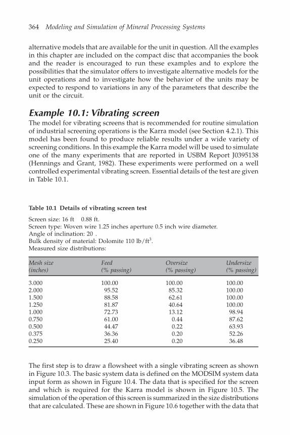
364 Modeling and Simulation of Mineral Processing Systems
alternative models that are available for the unit in question. All the examplesin this chapter are included on the compact disc that accompanies the bookand the reader is encouraged to run these examples and to explore thepossibilities that the simulator offers to investigate alternative models for theunit operations and to investigate how the behavior of the units may beexpected to respond to variations in any of the parameters that describe theunit or the circuit.
Example 10.1: Vibrating screenThe model for vibrating screens that is recommended for routine simulationof industrial screening operations is the Karra model (see Section 4.2.1). Thismodel has been found to produce reliable results under a wide variety ofscreening conditions. In this example the Karra model will be used to simulateone of the many experiments that are reported in USBM Report J0395138(Hennings and Grant, 1982). These experiments were performed on a wellcontrolled experimental vibrating screen. Essential details of the test are givenin Table 10.1.
Table 10.1 Details of vibrating screen test
Screen size: 16 ft 0.88 ft.Screen type: Woven wire 1.25 inches aperture 0.5 inch wire diameter.Angle of inclination: 20 .Bulk density of material: Dolomite 110 lb/ft3.Measured size distributions:
Mesh size Feed Oversize Undersize(inches) (% passing) (% passing) (% passing)
3.000 100.00 100.00 100.002.000 95.52 85.32 100.001.500 88.58 62.61 100.001.250 81.87 40.64 100.001.000 72.73 13.12 98.940.750 61.00 0.44 87.620.500 44.47 0.22 63.930.375 36.36 0.20 52.260.250 25.40 0.20 36.48
The first step is to draw a flowsheet with a single vibrating screen as shownin Figure 10.3. The basic system data is defined on the MODSIM system datainput form as shown in Figure 10.4. The data that is specified for the screenand which is required for the Karra model is shown in Figure 10.5. Thesimulation of the operation of this screen is summarized in the size distributionsthat are calculated. These are shown in Figure 10.6 together with the data that
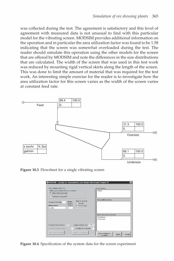
Simulation of ore dressing plants 365
was collected during the test. The agreement is satisfactory and this level ofagreement with measured data is not unusual to find with this particularmodel for the vibrating screen. MODSIM provides additional information onthe operation and in particular the area utilization factor was found to be 1.58indicating that the screen was somewhat overloaded during the test. Thereader should simulate this operation using the other models for the screenthat are offered by MODSIM and note the differences in the size distributionsthat are calculated. The width of the screen that was used in this test workwas reduced by mounting rigid vertical skirts along the length of the screen.This was done to limit the amount of material that was required for the testwork. An interesting simple exercise for the reader is to investigate how thearea utilization factor for this screen varies as the width of the screen variesat constant feed rate.
Feed
99.4 100.0
0.
s ton/hr % Sol
gal/min
31.3 100.0
0.
Oversize
68.1 100.0
0.
Undersize
Figure 10.3 Flowsheet for a single vibrating screen
Figure 10.4 Specification of the system data for the screen experiment

366 Modeling and Simulation of Mineral Processing Systems
The data used in the next three examples are taken from ICRA (1995).These data resulted from closely controlled sampling campaigns on the ballmill circuit of Noranda’s Geco mine. In the next two examples, the behaviorof the hydrocyclone classifier and the ball mill are simulated as isolatedsingle units and then the closed ball mill circuit is simulated. Finally thechanges that can be expected in the performance of the milling circuit aredetermined by simulation when the sizes of the vortex finder and apex of the
Figure 10.5 Parameter specification for the Karra screen model
Figure 10.6 Simulated size distribution compared to the data that were measuredduring the screening test
1 Feed 3 Undersize 2 Oversize100
90
80
70
60
50
40
30
20
10
010–1 100 101
Particle size cms
Cum
ulat
ive
% s
mal
ler

Simulation of ore dressing plants 367
hydrocyclone classifier are changed. The closed ball mill circuit is probablythe most common subject of simulation in mineral processing and a numberof variations of the ball mill model are available in MODSIM. For the purposesof this example we use a model that is based on the Herbst-Fuerstenau methodfor the calculation of the specific rate of breakage. This is appropriate in thiscase because the power drawn by the mill was measured during the samplingcampaigns.
Example 10.2: Hydrocyclone classifierThis example demonstrates the use of the simulator to match the simulationto the actual operation of the cyclone in the milling circuit. A simple flowsheetconsisting of a single hydrocyclone is set up in MODSIM as shown in Figure10.7. The particle size distribution and flowrate of the hydrocyclone feed isspecified as shown in Figure 10.8. The parameters for the hydrocyclone modelare specified as shown in Figure 10.9. The simulated particle-size distributionsare compared with the measured data in Figure 10.10. The Plitt model wasused to model the behavior of the hydrocyclone (see Section 4.5.7). In orderto accurately represent the measured data, the three calibration parametersfor this model were set to 1.00 for d50c, 0.36 for the sharpness factor and 2.0 forthe flow split factor. These adjustments to the standard model indicate that
Figure 10.7 Flowsheet for single hydrocyclone
163.2 51.4
154.4
Primary cyclone overflow
418.0 66.9
206.8
Primary cyclone feed
tonne/hr % Sol
tonne/h
254.8
52.4
82.9
Primary cyclone underflow
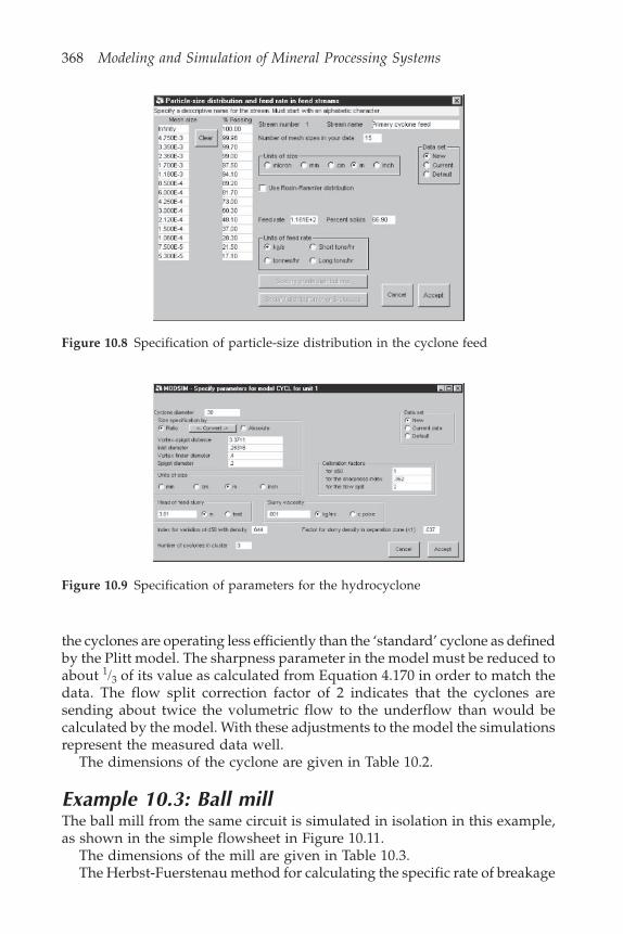
368 Modeling and Simulation of Mineral Processing Systems
the cyclones are operating less efficiently than the ‘standard’ cyclone as definedby the Plitt model. The sharpness parameter in the model must be reduced toabout 1/3 of its value as calculated from Equation 4.170 in order to match thedata. The flow split correction factor of 2 indicates that the cyclones aresending about twice the volumetric flow to the underflow than would becalculated by the model. With these adjustments to the model the simulationsrepresent the measured data well.
The dimensions of the cyclone are given in Table 10.2.
Example 10.3: Ball millThe ball mill from the same circuit is simulated in isolation in this example,as shown in the simple flowsheet in Figure 10.11.
The dimensions of the mill are given in Table 10.3.The Herbst-Fuerstenau method for calculating the specific rate of breakage
Figure 10.8 Specification of particle-size distribution in the cyclone feed
Figure 10.9 Specification of parameters for the hydrocyclone

Simulation of ore dressing plants 369
1 Primary cyclone feed 3 Primary cyclone underflow 2 Primary cyclone overflow
100
90
80
70
60
50
40
30
20
10
010 100 1000 10000
Particle size, microns
Cum
ulat
ive
% s
mal
ler
is used because the power drawn by the mill is known. The data for this millmodel is specified as shown in Figure 10.12.
Figure 10.10 Simulated particle-size distributions compared to the measured data
Table 10.2 Dimensions of the hydrocyclone
Diameter 0.38 mInlet diameter 0.1 mVortex finder diameter 0.152 mApex diameter 0.076 mCylinder length 0.28 mCone angle 15
Ball mill feed Ball mill discharge
Figure 10.11 Simple flowsheet for a single ball mill
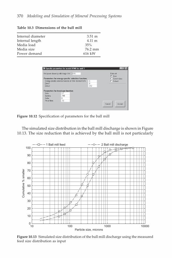
370 Modeling and Simulation of Mineral Processing Systems
1 Ball mill feed 2 Ball mill discharge100
90
80
70
60
50
40
30
20
10
010 100 1000 10000
Particle size, microns
Cum
ulat
ive
% s
mal
ler
The simulated size distribution in the ball mill discharge is shown in Figure10.13. The size reduction that is achieved by the ball mill is not particularly
Table 10.3 Dimensions of the ball mill
Internal diameter 3.51 mInternal length 4.11 mMedia load 35%Media size 76.2 mmPower demand 616 kW
Figure 10.12 Specification of parameters for the ball mill
Figure 10.13 Simulated size distribution of the ball mill discharge using the measuredfeed size distribution as input

Simulation of ore dressing plants 371
large in this example and the circuit relies on the recirculating load to producea sufficiently fine product.
Example 10.4: Rod and ball mill circuitThe two units that were simulated in Examples 10.2 and 10.3 are now combinedinto a closed ball milling circuit and an open circuit rod mill is added toproduce the feed to the ball mill circuit. This flowsheet now matches theplant from which the data were obtained. The dimensions of the hydrocycloneand the ball mill are given in Tables 10.2 and 10.3 and those of the rod mill aregiven in Table 10.4.
Table 10.4 Dimensions of the rod mill
Internal diameter 3.51 mInternal length 4.11 mMedia load 35%Media size 89 mmPower demand 560 kW
Sump water
Rod mill
tonne/hrtonne/hr
% Sol Sump
294.328.5
91.2
Ball mill discharge
Ball mill
Cyclone underflow
294.528.5
91.2
Hydrocyclone
Cyclone overflow
160.1344.9
31.7
Figure 10.14 Rod and ball mill circuit
The closed milling circuit shown in Figure 10.14 and the simulated sizedistributions around the circuit are shown in Figure 10.15.
The models used lead to a good simulation of the size distributions aroundthe circuit.
10.5 Integrated flowsheetsIn this section we simulate a few integrated flowsheets and show how themodels work together to simulate complex plants.
6
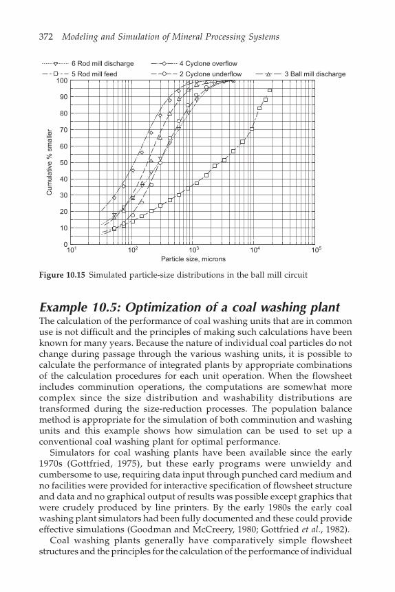
372 Modeling and Simulation of Mineral Processing Systems
6 Rod mill discharge
5 Rod mill feed
4 Cyclone overflow
2 Cyclone underflow 3 Ball mill discharge100
90
80
70
60
50
40
30
20
10
0101 102 103 104 105
Particle size, microns
Cum
ulat
ive
% s
mal
ler
Example 10.5: Optimization of a coal washing plantThe calculation of the performance of coal washing units that are in commonuse is not difficult and the principles of making such calculations have beenknown for many years. Because the nature of individual coal particles do notchange during passage through the various washing units, it is possible tocalculate the performance of integrated plants by appropriate combinationsof the calculation procedures for each unit operation. When the flowsheetincludes comminution operations, the computations are somewhat morecomplex since the size distribution and washability distributions aretransformed during the size-reduction processes. The population balancemethod is appropriate for the simulation of both comminution and washingunits and this example shows how simulation can be used to set up aconventional coal washing plant for optimal performance.
Simulators for coal washing plants have been available since the early1970s (Gottfried, 1975), but these early programs were unwieldy andcumbersome to use, requiring data input through punched card medium andno facilities were provided for interactive specification of flowsheet structureand data and no graphical output of results was possible except graphics thatwere crudely produced by line printers. By the early 1980s the early coalwashing plant simulators had been fully documented and these could provideeffective simulations (Goodman and McCreery, 1980; Gottfried et al., 1982).
Coal washing plants generally have comparatively simple flowsheetstructures and the principles for the calculation of the performance of individual
Figure 10.15 Simulated particle-size distributions in the ball mill circuit
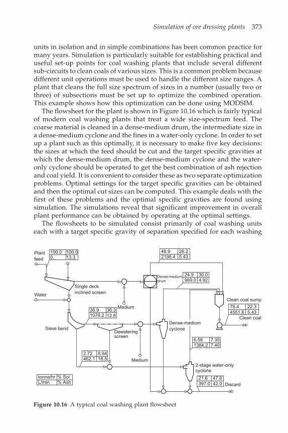
Simulation of ore dressing plants 373
units in isolation and in simple combinations has been common practice formany years. Simulation is particularly suitable for establishing practical anduseful set-up points for coal washing plants that include several differentsub-circuits to clean coals of various sizes. This is a common problem becausedifferent unit operations must be used to handle the different size ranges. Aplant that cleans the full size spectrum of sizes in a number (usually two orthree) of subsections must be set up to optimize the combined operation.This example shows how this optimization can be done using MODSIM.
The flowsheet for the plant is shown in Figure 10.16 which is fairly typicalof modern coal washing plants that treat a wide size-spectrum feed. Thecoarse material is cleaned in a dense-medium drum, the intermediate size ina dense-medium cyclone and the fines in a water-only cyclone. In order to setup a plant such as this optimally, it is necessary to make five key decisions:the sizes at which the feed should be cut and the target specific gravities atwhich the dense-medium drum, the dense-medium cyclone and the water-only cyclone should be operated to get the best combination of ash rejectionand coal yield. It is convenient to consider these as two separate optimizationproblems. Optimal settings for the target specific gravities can be obtainedand then the optimal cut sizes can be computed. This example deals with thefirst of these problems and the optimal specific gravities are found usingsimulation. The simulations reveal that significant improvement in overallplant performance can be obtained by operating at the optimal settings.
The flowsheets to be simulated consist primarily of coal washing unitseach with a target specific gravity of separation specified for each washing
Figure 10.16 A typical coal washing plant flowsheet
100.0 100.00. 13.3
Plantfeed
Water
Single deckinclined screen
Medium36.91078.2
36.312.8
Dewateringscreen
Medium2.72462.1
8.9418.5
tonne/hrL/min
% Sol% Ash
Sieve bend
2198.4 5.4346.9 26.2
Dense-mediumdrum
24.9969.0
30.04.92
78.44551.6
22.35.43
Clean coal sump
Clean coal
6.581384.2
7.357.40
2-stage water-onlycyclone
21.6397.0
47.642.0 Discard
Dense-mediumcyclone

374 Modeling and Simulation of Mineral Processing Systems
unit. The feed is allocated to each washing unit on the basis of separation bysize in the screening operations. The target specific gravity of separation inany unit is the separation point to be expected when the partition curve ofthe composite feed to clean coal is plotted without considering each narrowsize fraction separately. All gravity separation units are known to showsignificant variation of separation performance as a function of particle size.In general the cut point increases with decreasing particle size and the efficiencyof separation decreases with decreasing particle size. This is particularlynoticeable at particle sizes smaller than a few millimeters – so-called fine coalseparations.
The cut point can be controlled by variation of an operational control inthe plant or by means of a physical adjustment to the equipment. Dense-medium separators are set by controlling the medium density and theseparation density in autogenous separators such as water-only cyclones,concentrating tables and jigs are controlled by physical adjustments. At thehighest level, simulation models should accept as input data a specificationof the equipment type and the settings of all controllable physical variablesand be capable of predicting the cut points and separation efficiencies thatwill be achieved in practice. Models at this level are not always available andusually require careful calibration against pilot or full-scale plant data. In thepresent case no suitable data are available to calibrate high-level models andmore restricted models which accept a target cut point are used for thesimulation. Models that use this principle are described in Section 7.4.
To assess the efficacy of the optimization procedure, the plant was simulatedusing the target specific gravities in the dense-medium drum, the dense-medium cyclone and the water-only cyclone that are currently set up in theplant. This is the base case against which the optimum solution can be judged.The base case specified target cut points of 1.35, 1.65 and 1.95 in the dense-medium drum, dense-medium cyclone and water-only cyclone respectively.
Before the plant can be optimized, it is necessary to investigate theperformance of each of the individual washing units under conditions that itexperiences during operation within the plant flowsheet. This is the first taskof the simulator which can be used to investigate the range of performance ofeach washing unit in the plant. The performance of each washing unit inflowsheet 10.16 was simulated over a range of target cut points. The resultsare summarized in Figure 10.17. The figure shows the cumulative yield againstthe cumulative ash for each of the three washing units together with thetheoretical yields calculated from the washability data of the feed material toeach unit.
The arrangement of three separation units in parallel lends itself tooptimization so that the plant can produce clean coal at the greatest possibleyield at a given ash content or at the minimum ash content for a given yield.The optimal combination of target cut points for the three washing units iseasy to establish in this case using the simulated data from Figure 10.17. Thecalculated yields are replotted as the product of yield ash content versusyield for each of the three units as shown in Figure 10.18. Each calculated
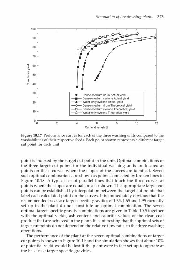
Simulation of ore dressing plants 375
100
90
80
70
60
50
40
30
20
10
00 2 4 6 8 10 12
Cumulative ash %
Cum
ulat
ive
yiel
d
Dense-medium drum Actual yieldDense-medium cyclone Actual yieldWater-only cyclone Actual yieldDense-medium drum Theoretical yieldDense-medium cyclone Theoretical yieldWater-only cyclone Theoretical yield
point is indexed by the target cut point in the unit. Optimal combinations ofthe three target cut points for the individual washing units are located atpoints on these curves where the slopes of the curves are identical. Sevensuch optimal combinations are shown as points connected by broken lines inFigure 10.18. A typical set of parallel lines that touch the three curves atpoints where the slopes are equal are also shown. The appropriate target cutpoints can be established by interpolation between the target cut points thatlabel each calculated point on the curves. It is immediately obvious that therecommended base case target specific gravities of 1.35, 1.65 and 1.95 currentlyset up in the plant do not constitute an optimal combination. The sevenoptimal target specific gravity combinations are given in Table 10.5 togetherwith the optimal yields, ash content and calorific values of the clean coalproduct that are achieved in the plant. It is interesting that the optimal sets oftarget cut points do not depend on the relative flow rates to the three washingoperations.
The performance of the plant at the seven optimal combinations of targetcut points is shown in Figure 10.19 and the simulation shows that about 10%of potential yield would be lost if the plant were in fact set up to operate atthe base case target specific gravities.
Figure 10.17 Performance curves for each of the three washing units compared to thewashabilities of their respective feeds. Each point shown represents a different targetcut point for each unit

376 Modeling and Simulation of Mineral Processing Systems
Figure 10.18 Ash-yield products for the three individual washing units. Points wherethese curves have equal slopes define optimal combinations of target specific gravities
Figure 10.19 Optimal performance curve for the plant compared to the washabilityof the feed and to the base case which is suboptimal
100
90
80
70
60
50
40
30
20
10
00 2 4 6 8 10 12
Plant with optimal settingsWashability of the feedPlant operating at recommended settings
Cumulative ash %
Opt
imal
yie
ld %
Yield ash for the dense-medium drumYield ash for the DMCYYield ash for water-only cycloneDense-medium drum. Recommended settingDense-medium cyclone. Recommended settingWater-only cyclone. Recommended settingContours connecting optimal settings
12
10
8
6
4
2
0
Yie
ld
ash
30 40 50 60 70 80 90 100
1.31.331.35
1.36 1.41.45
1.5
1.6
1.7
1.8
1.9
2.0
1.91.8
1.7
1.6
1.51.45
1.41.36
1.351.33
1.31.3
1.331.35
1.36
1.4
1.45
1.51.61.7
1.81.9
2.0
Cumulative yield %
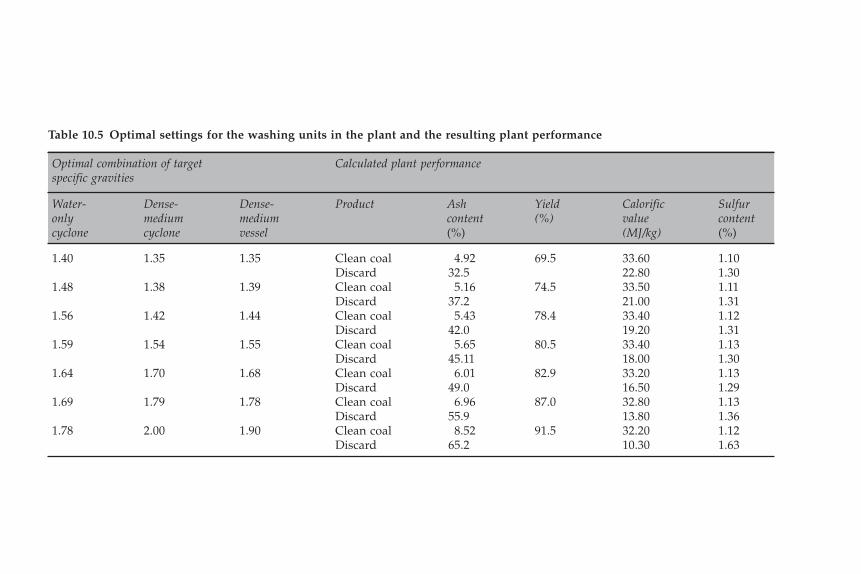
Table 10.5 Optimal settings for the washing units in the plant and the resulting plant performance
Optimal combination of target Calculated plant performancespecific gravities
Water- Dense- Dense- Product Ash Yield Calorific Sulfuronly medium medium content (%) value contentcyclone cyclone vessel (%) (MJ/kg) (%)
1.40 1.35 1.35 Clean coal 4.92 69.5 33.60 1.10Discard 32.5 22.80 1.30
1.48 1.38 1.39 Clean coal 5.16 74.5 33.50 1.11Discard 37.2 21.00 1.31
1.56 1.42 1.44 Clean coal 5.43 78.4 33.40 1.12Discard 42.0 19.20 1.31
1.59 1.54 1.55 Clean coal 5.65 80.5 33.40 1.13Discard 45.11 18.00 1.30
1.64 1.70 1.68 Clean coal 6.01 82.9 33.20 1.13Discard 49.0 16.50 1.29
1.69 1.79 1.78 Clean coal 6.96 87.0 32.80 1.13Discard 55.9 13.80 1.36
1.78 2.00 1.90 Clean coal 8.52 91.5 32.20 1.12Discard 65.2 10.30 1.63

378 Modeling and Simulation of Mineral Processing Systems
The coal washability data is entered in the simulator as shown in Figure 10.20.
Data completionThe data available for this simulation was incomplete in two important respectsand required completion. The effective densities of the two outer washabilityfractions were not given and the washability analysis of the 200 mesh 0 sizefraction was missing. These omissions are commonly found in coal washabilitydata sets. The effective densities of the outer washability fractions determinethe behavior of this material that is predicted by the unit models and arational assignment of effective density is necessary particularly when theunits will be set up to cut at either high or low specific gravities. The washabilitydistribution of the 200 mesh 0 fraction was estimated by assuming that thelower nine density fractions were distributed identically to the those in the
Table 10.6 The properties of the raw coal used in the simulation
(a) Raw-coal size distribution
SizeWeight Ash
Passed Retained (wt%) (wt%)
1 12 in. 15.8 18.12
1 12 in. 3
4 in. 22.5 13.44
34 in. 3
8 in. 18.2 12.17
38 in. 28 mesh 33.2 11.08
28 mesh 100 mesh 4.5 10.88100 mesh 200 mesh 1.7 12.25200 mesh 4.1 27.07
(b) Raw-coal analysis
Specific gravityHeating
Sink Float Representative Ash Sulfur valuevalue (wt %) (wt %) (Btu/lb)
1.30 1.299 2.96 0.99 148121.30 1.35 1.325 5.93 1.13 142871.35 1.40 1.375 11.04 1.83 133501.40 1.45 1.425 16.07 1.68 125021.45 1.50 1.475 22.78 1.26 114241.50 1.60 1.550 28.99 0.91 103861.60 1.70 1.650 36.43 0.83 91221.70 1.80 1.750 45.71 0.58 74931.80 2.17 1.985 58.99 0.88 52962.17 2.500 81.52 2.38 1850

(c) Raw coal size-by-size washability
Specific gravity 1 12 1 1
234
34
38
38 28 mesh 28 100 mesh 100 200 mesh 200 0
Weight Weight Weight Weight Weight Weight WeightSink Float (wt %) (wt %) (wt %) (wt %) (wt %) (wt %) (wt %)
1.30 37.7 42.4 41.0 50.3 63.0 60.7 48.941.30 1.35 31.1 28.0 30.1 23.4 14.2 12.9 10.401.35 1.40 1.9 7.4 9.0 8.1 5.9 4.0 3.221.40 1.45 1.4 2.9 4.4 4.3 3.2 4.9 3.951.45 1.50 2.4 2.0 1.9 1.7 1.4 2.1 1.691.50 1.60 4.0 5.4 3.6 2.4 2.2 2.9 2.341.60 1.70 3.7 3.4 2.4 1.7 1.3 1.7 1.371.70 1.80 2.9 1.9 1.8 1.4 0.9 1.0 0.811.80 2.17 9.0 4.0 3.3 2.8 2.4 2.7 2.182.17 5.9 2.6 2.5 3.9 5.5 7.1 25.10
Table 10.6 (Cont’d.)
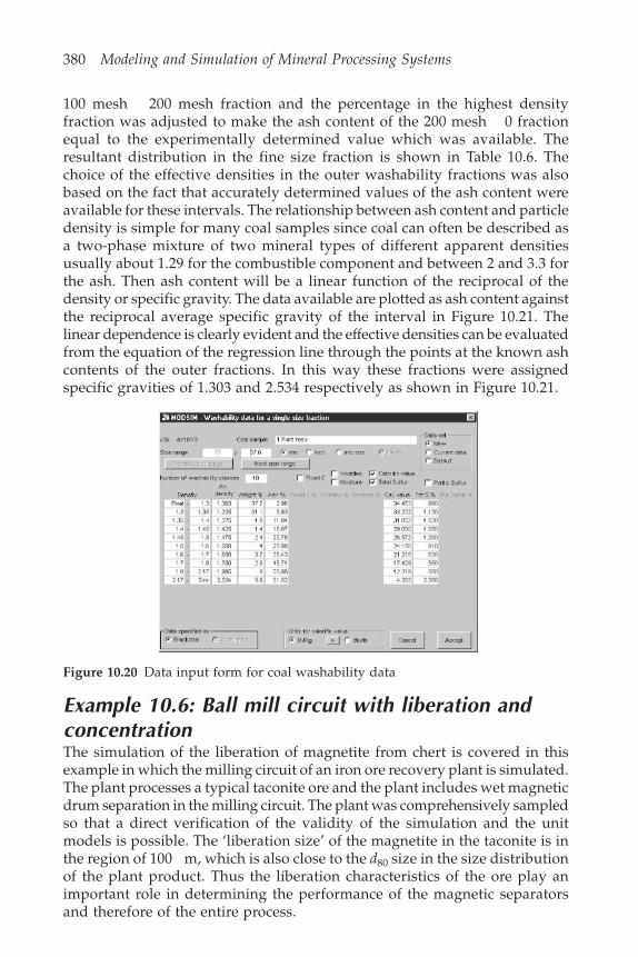
380 Modeling and Simulation of Mineral Processing Systems
100 mesh 200 mesh fraction and the percentage in the highest densityfraction was adjusted to make the ash content of the 200 mesh 0 fractionequal to the experimentally determined value which was available. Theresultant distribution in the fine size fraction is shown in Table 10.6. Thechoice of the effective densities in the outer washability fractions was alsobased on the fact that accurately determined values of the ash content wereavailable for these intervals. The relationship between ash content and particledensity is simple for many coal samples since coal can often be described asa two-phase mixture of two mineral types of different apparent densitiesusually about 1.29 for the combustible component and between 2 and 3.3 forthe ash. Then ash content will be a linear function of the reciprocal of thedensity or specific gravity. The data available are plotted as ash content againstthe reciprocal average specific gravity of the interval in Figure 10.21. Thelinear dependence is clearly evident and the effective densities can be evaluatedfrom the equation of the regression line through the points at the known ashcontents of the outer fractions. In this way these fractions were assignedspecific gravities of 1.303 and 2.534 respectively as shown in Figure 10.21.
Figure 10.20 Data input form for coal washability data
Example 10.6: Ball mill circuit with liberation andconcentrationThe simulation of the liberation of magnetite from chert is covered in thisexample in which the milling circuit of an iron ore recovery plant is simulated.The plant processes a typical taconite ore and the plant includes wet magneticdrum separation in the milling circuit. The plant was comprehensively sampledso that a direct verification of the validity of the simulation and the unitmodels is possible. The ‘liberation size’ of the magnetite in the taconite is inthe region of 100 m, which is also close to the d80 size in the size distributionof the plant product. Thus the liberation characteristics of the ore play animportant role in determining the performance of the magnetic separatorsand therefore of the entire process.

Simulation of ore dressing plants 381
A simplified flowsheet of the plant is shown in Figure 10.22. The feed tothe grinding circuit consists mainly of a concentrate stream from cobbermagnetic separators which concentrate the rod mill discharge from the primarygrinding stage. The ball mill circuit is closed with a hydrocyclone and itincludes a rougher magnetic separator in the ball mill discharge. The circuitis complicated further by feed back of water and solids from a dewateringdrum magnetic separator. The magnetic rougher tails are cleaned in a scavengermagnetic separator and the concentrate from this scavenger is fed to thecyclone feed sump together with the rougher concentrate. The performanceof the magnetic separator depends strongly on the magnetite content ofindividual particles, which in turn is dominated by the liberation processesthat occur in the ball mill.
This plant cannot be characterized only by the size distributions of thevarious process streams. The liberation distributions are equally important.Samples were collected from the plant during a period of normal operationand the size and liberation distributions at each size were measured. The sizedistributions were measured using standard sieve analysis and the liberationspectra were determined by image analysis using the linear intercept methodand appropriate stereological transformation. The image analysis techniqueused for the measurement of the liberation spectra is described in Chapter 2and the liberation spectra measured in the four plant feed streams (cobberconcentrate, dewatering drum concentrate, dewatering drum tails andscavenger concentrate) are shown in Figures 10.23 to 10.26. The compositionof these streams and the distribution of liberated and unliberated particles is
Measured mineral matter content in heaviest fraction100
90
80
70
60
50
40
30
20
10
00.3 0.4 0.5 0.6 0.7 0.8
Reciprocal of specific gravity
Min
eral
mat
ter
89.35
0.3945 0.768 3.74
Measured mineral matter in lightest fraction
Figure 10.21 Extrapolation to find the effective density of the two outer washabilityfractions
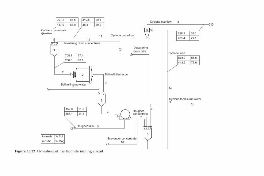
Figure 10.22 Flowsheet of the taconite milling circuit
301.2 68.6
137.9 55.0
349.5 90.1
38.4 69.0
Cobber concentrate
1
1
Dewatering drum concentrate12
11 Cyclone underflow
6
8Cyclone overflow
228.9
405.4
36.1
79.1
578.2
443.9
56.6
73.0
Cyclone feed
14
9Cyclone feed sump water
13
7
Rougherconcentrate
4
4
5
10Scavenger concentrate
5Rougher tails
tonne/hr
m^3/hr
% Sol
% Mag
152.0
555.1
21.5
24.1
3
3Ball mill sump water6
2 Ball mill discharge2
708.1
206.6
77.4
63.1
Dewateringdrum tails
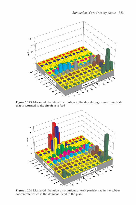
Simulation of ore dressing plants 383
Figure 10.23 Measured liberation distribution in the dewatering drum concentratethat is returned to the circuit as a feed
Figure 10.24 Measured liberation distributions at each particle size in the cobberconcentrate which is the dominant feed to the plant

384 Modeling and Simulation of Mineral Processing Systems
Figure 10.25 Measured liberation distribution at each particle size in the dewateringdrum tails which is returned to the circuit as a feed
Figure 10.26 Measured liberation distributions in the scavenger concentrate whichis returned to the circuit as a feed

Simulation of ore dressing plants 385
clearly evident form these graphs. Note in particular the absence of liberatedmagnetite in the dewatering drum tails and the small amounts of liberatedchert in the dewatering drum concentrate and the scavenger concentrate.This liberated chert is returned from these units by entrainment of the chertwith the magnetite on the drum separators. This is typical of the operation ofwet drum magnetic separators.
The plant was simulated with these feed streams using the Austin modelfor the ball mill including the Andrews-Mika diagram method to simulatethe liberation that occurs during grinding. The liberation data is entered intoMODSIM using the data input screen as shown in Figures 10.27 and 10.28.
The results of the simulation can be compared to the actual plant behaviorby comparing the calculated particle-size distributions and the liberationdistributions in each of the sampled streams. The comparison of the particle-size distributions is shown in Figure 10.29. The liberation distributions arecompared in Figures 10.30 to 10.41.
Figure 10.27 Specification of the grade classes in MODSIM
Figure 10.28 Specification of the liberation distribution in the feed stream

386 Modeling and Simulation of Mineral Processing Systems
Figure 10.29 Comparison between calculated and measured size distributions infive plant streams. Plotted points are measured and the lines are calculated by thesimulation
It is obvious from these graphs that the simulator provides a goodrepresentation of both the size distributions and the liberation distributionsin this plant. The matches between measured and simulated data are excellent.
The measured and simulated data make it possible to diagnose severalimportant aspects of the plant operation. Figures 10.38 and 10.39 show thecharacter of the final product from the circuit in the cyclone overflow. Thismaterial is comparatively fine with a d80 size of 82 m and both the measuredand simulated data indicate that the final product is largely fine liberatedmagnetite, which is the desired product. However there is a small componentof incompletely liberated particles in the size range 75 m to 250 m. This isthe largest source of silica contamination in the product. Some reduction inthe cut size that is achieved in the hydrocyclone could be beneficial.
The character of the particles in the hydrocyclone underflow is of particularinterest in this plant. The measured and simulated liberation distributionsare shown in Figures 10.36 and 10.37. It is clear that the hydrocyclones arereturning coarse material to the mill as they should and that this material ismostly unliberated. This material is reground in the mill and will eventuallyleave the circuit as fine liberated magnetite. However the hydrocyclone isalso returning liberated magnetite in significant amounts to the mill, and thatis wasteful because excess energy is required in the mill to grind alreadyliberated material. This liberated magnetite enters the hydrocyclone underflowbecause it has a density significantly greater than that of the chert.
Particle size, microns
5 Rougher tails
8 Cyclone overflow
1 Cobber concentrate
11 Cyclone underflow3 Ball mill discharge
7 Rougher concentrate
14 Cyclone feed100
90
80
70
60
50
40
30
20
10
00 10 100 1000 10000
Cum
ulat
ive
% s
mal
ler
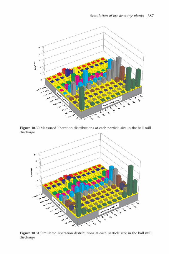
Simulation of ore dressing plants 387
Figure 10.31 Simulated liberation distributions at each particle size in the ball milldischarge
Figure 10.30 Measured liberation distributions at each particle size in the ball milldischarge
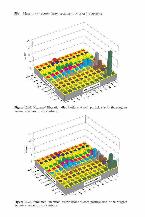
388 Modeling and Simulation of Mineral Processing Systems
Figure 10.33 Simulated liberation distributions at each particle size in the roughermagnetic separator concentrate
Figure 10.32 Measured liberation distributions at each particle size in the roughermagnetic separator concentrate
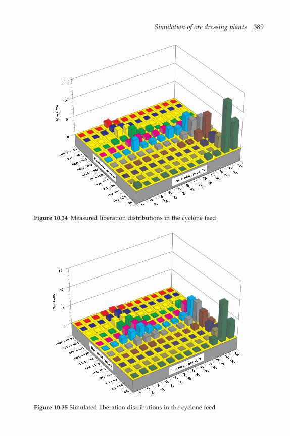
Simulation of ore dressing plants 389
Figure 10.35 Simulated liberation distributions in the cyclone feed
Figure 10.34 Measured liberation distributions in the cyclone feed
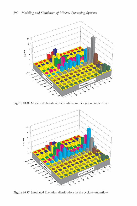
390 Modeling and Simulation of Mineral Processing Systems
Figure 10.37 Simulated liberation distributions in the cyclone underflow
Figure 10.36 Measured liberation distributions in the cyclone underflow
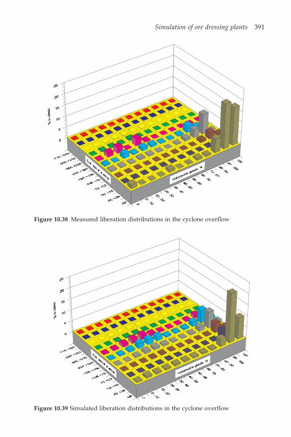
Simulation of ore dressing plants 391
Figure 10.39 Simulated liberation distributions in the cyclone overflow
Figure 10.38 Measured liberation distributions in the cyclone overflow
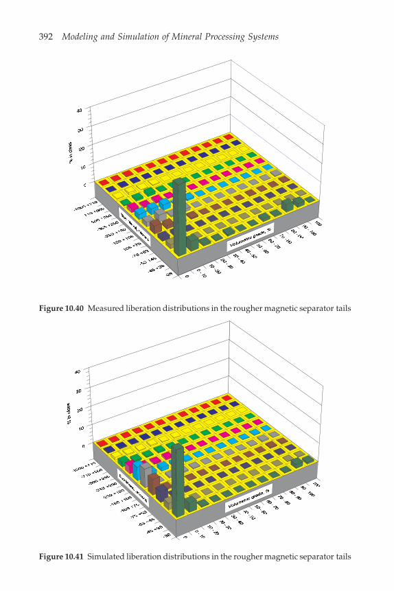
392 Modeling and Simulation of Mineral Processing Systems
Figure 10.41 Simulated liberation distributions in the rougher magnetic separator tails
Figure 10.40 Measured liberation distributions in the rougher magnetic separator tails
Simulation of ore dressing plants 393
The reader is encouraged to run this simulation and investigate possiblestrategies to improve the performance of the circuit. The main objective shouldbe to reduce the energy consumption without reducing the recovery or thegrade of the final product. The wasteful recirculation of liberated magnetitecan be addressed by using fine screens rather than hydrocyclones forclassification and this can be easily investigated using the simulator. A completeaccount of this simulation project can be found in Schneider (1995).
10.6 Symbols used in this chapterE Unit recovery matrix.F Composite vector of mass flowrates in the plant feed streams.I Identity matrix.P Composite vector of mass flowrates in the plant product streams.T Unit transformation matrix.W Vector of mass flowrates in a stream.X Composite vector of assumed mass flowrates in the tear streams.Y Composite vector of calculated mass flowrates in the tear streams.� Composite matrix representing calculation paths from feed streams to
product streams.� Composite matrix representing calculation paths from tear streams to
product streams.� Composite matrix representing calculation paths from tear streams back
to tear streams.� Composite matrix representing calculation paths from feed streams to
tear streams.
ReferencesFord, M.A. (1979) Simulation of Ore dressing Plants. Ph.D Thesis, University of the
Witwatersrand, Johannesburg.Goodman, F.K. and McCreery, J.H. (1988) Coal Preparation Plant Computer Model
Vols I and II. U.S. Environment Protection Agency EPA-600/7-80-010 a & b.Gottfried, B.S. (1975) Computer Simulation of Coal Preparation Plants. U.S. Bureau of
Mines, Grant No. GO-155030 Final Report, Dept of Industrial Engineering, Univ. ofPittsburgh, Nov 1975 and August 1977.
Gottfried, B.S. and Jacobsen, P.S. (1977) Generalized Distribution Curve forCharacterizing the Performance of Coal-Cleaning Equipment USBM RI 8238.
Gottfried, B.S., Luckie, P.T. and Tierney, J.W. (1982) Computer Simulation of CoalPreparation Plants. U.S. Dept of Energy Final Report under contract AC22-80PC30144.DOE/PC/30144-T7, 284 pp.
Hennings, K. and Grant, D. (1982) A simulation model for the prediction of theperformance of vibrating screens. USBM Contract J0395138, U.S. Department ofthe Interior. Washington D.C.
ICRA (1995) Simulation of Comminution Operations. Standard Problems for Simulators.International Comminution Research Association. 5th Workshop, Napa.

394 Modeling and Simulation of Mineral Processing Systems
King, R.P. (1972) Data preparation and use of a computer program for the calculationof the performance of a flotation plant. National Institute for Metallurgy (nowMintek), Johannesburg, Report number 1436, 9 pp. Reissued in revised form August1973.
King, R.P., Pugh, G. and Langley, J. (1973) Application of a flotation model to anindustrial plant. National Institute for Metallurgy (now Mintek), Johannesburg.Report number 1562, 16 pp.
Schneider, C.L. (1995) The Measurement and Calculation of Liberation in ContinuousGrinding Circuits. Ph.D Thesis. University of Utah.
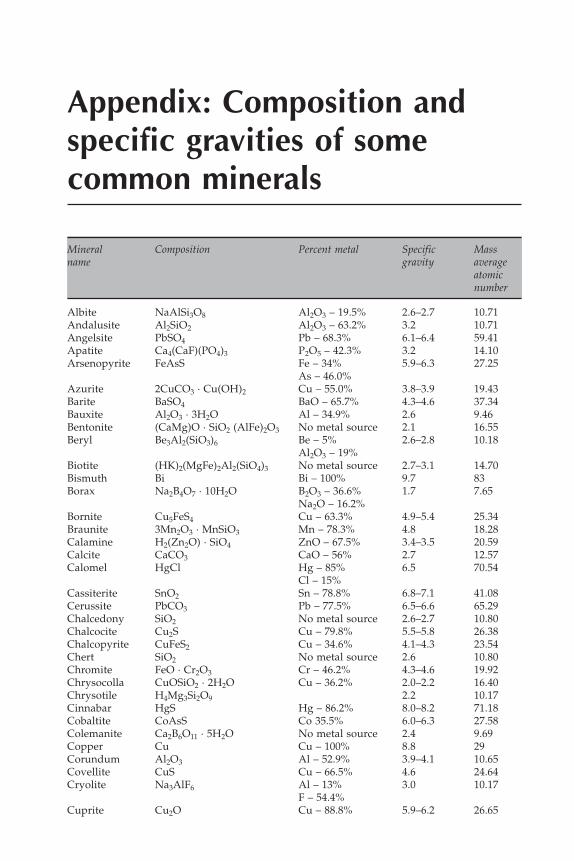
Appendix: Composition andspecific gravities of somecommon minerals
Mineral Composition Percent metal Specific Massname gravity average
atomicnumber
Albite NaAlSi3O8 Al2O3 – 19.5% 2.6–2.7 10.71Andalusite Al2SiO2 Al2O3 – 63.2% 3.2 10.71Angelsite PbSO4 Pb – 68.3% 6.1–6.4 59.41Apatite Ca4(CaF)(PO4)3 P2O5 – 42.3% 3.2 14.10Arsenopyrite FeAsS Fe – 34% 5.9–6.3 27.25
As – 46.0%Azurite 2CuCO3 · Cu(OH)2 Cu – 55.0% 3.8–3.9 19.43Barite BaSO4 BaO – 65.7% 4.3–4.6 37.34Bauxite Al2O3 · 3H2O Al – 34.9% 2.6 9.46Bentonite (CaMg)O · SiO2 (AlFe)2O3 No metal source 2.1 16.55Beryl Be3Al2(SiO3)6 Be – 5% 2.6–2.8 10.18
Al2O3 – 19%Biotite (HK)2(MgFe)2Al2(SiO4)3 No metal source 2.7–3.1 14.70Bismuth Bi Bi – 100% 9.7 83Borax Na2B4O7 · 10H2O B2O3 – 36.6% 1.7 7.65
Na2O – 16.2%Bornite Cu5FeS4 Cu – 63.3% 4.9–5.4 25.34Braunite 3Mn2O3 · MnSiO3 Mn – 78.3% 4.8 18.28Calamine H2(Zn2O) · SiO4 ZnO – 67.5% 3.4–3.5 20.59Calcite CaCO3 CaO – 56% 2.7 12.57Calomel HgCl Hg – 85% 6.5 70.54
Cl – 15%Cassiterite SnO2 Sn – 78.8% 6.8–7.1 41.08Cerussite PbCO3 Pb – 77.5% 6.5–6.6 65.29Chalcedony SiO2 No metal source 2.6–2.7 10.80Chalcocite Cu2S Cu – 79.8% 5.5–5.8 26.38Chalcopyrite CuFeS2 Cu – 34.6% 4.1–4.3 23.54Chert SiO2 No metal source 2.6 10.80Chromite FeO · Cr2O3 Cr – 46.2% 4.3–4.6 19.92Chrysocolla CuOSiO2 · 2H2O Cu – 36.2% 2.0–2.2 16.40Chrysotile H4Mg3Si2O9 2.2 10.17Cinnabar HgS Hg – 86.2% 8.0–8.2 71.18Cobaltite CoAsS Co 35.5% 6.0–6.3 27.58Colemanite Ca2B6O11 · 5H2O No metal source 2.4 9.69Copper Cu Cu – 100% 8.8 29Corundum Al2O3 Al – 52.9% 3.9–4.1 10.65Covellite CuS Cu – 66.5% 4.6 24.64Cryolite Na3AlF6 Al – 13% 3.0 10.17
F – 54.4%Cuprite Cu2O Cu – 88.8% 5.9–6.2 26.65

396 Modeling and Simulation of Mineral Processing Systems
Diamond C C – 100% 3.5 6Dolomite CaMg(CO3)2 CaO – 30.4% 2.8–2.9 10.87
MgO – 21.9%Epsom salt MgSO4 · 7H2O Mg – 9.9% 1.7 9.03Fluorite CaF2 F – 48.9% 3.0–3.3 14.65Galena PbS Pb – 86.6% 7.4–7.6 73.15Garnet Various No metal source 3.2–4.3Garnierite H2(NiMg)SiO4 Ni – 25% to 30% 2.4 16.05Gibbsite Al(OH)3 Al – 34.6% 2.4 9.46Gold Au Au – 100% 15.6–19.3 79Graphite C C – 100% 2.2 6Gypsum CaSO4 · 2H2O CaO – 32.6% 2.3 12.12Halite NaCl Na – 39.4% 2.1–2.6 14.64Hausmannite Mn3O4 Mn – 72% 4.7 20.25Hematite Fe2O3 Fe – 70% 4.9–5.3 20.59Ilmenite FeTiO3 Ti – 31.6% 4.5–5.0 19.04Iridium Variable Variable 22.7 77.00Kaolinite H4Al2Si2O9 Al2O3 2.6 10.24Leucite KAl(SiO3)2 K2O – 21.5% 2.5 12.13
Al2O3 – 23.5%Limonite 2Fe2O3 · 2H2O Fe – 59.5% 3.6–4.0 18.65Magnesite MgCO3 Mg – 28.9% 3.1 8.87Magnetite FeO · Fe2O3 Fe – 72.4% 5.2 21.02Malachite CuCO3 · Cu(OH)2 Cu – 57.5% 4.0 19.90Manganite Mn2O3 · H2O Mn – 62.5% 4.2–4.4 18.54Marble Chiefly CaCO3 Ca – 40% 2.7 12.57Marcasite FeS2 Fe – 46.6% 4.9 20.66Marmatite (ZnFe)S variable Zn – 46.5% to 56.9% 3.9–4.2Mercury Hg Hg – 100% 13.59 80Molybdenite MoS2 Mo – 60% 4.7–4.8 31.58Monazite (CeLaDy)PO4 · ThSiO4 ThO2 – 9% 4.9–5.3 57.56Muscovite H2KAl3(SiO4)3 Variable 2.8–3.0 11.33Olivine (MgFe)2SiO4 No metal source 3.3 17.40Opal SiO2 · nH2O No metal source 1.9–2.3Orpiment As2S3 As – 61% 3.5 26.35Orthoclase KAlSi3O8 Al2O3 – 18.4% 2.5–2.6 11.85Pentlandite (FeNi)S Fe – 42.0% 4.6–5.0 24.61
Ni – 22.0%Platinum Pt Pt – 100% 17.0 78Pyrite FeS2 Fe – 46.7% 5.0 20.65Pyrolusite MnO2 Mn – 63.2% 4.8 18.74Pyrophyllite HAl(SiO3)2 Al2O3 – 28.3% 2.8–2.9 10.58Pyroxene Ca(AlMgMnFe)(SiO3)2 No metal source 3.3 16.437Pyrrhotite Fe5S6 to Fe16S17 Fe – 61.5% Variable 4.6 21.92 to
22.21Quartz SiO2 Si – 46.9% 2.65–2.66 10.80Realgar AsS As – 70.1% 2.6 27.90Ruby Al2O3 Al – 52.9% 4.0 10.65Rutile TiO2 Ti – 60% 4.2 16.39Scheelite CaWO4 W – 63.9% 4.9–6.1 51.81Serpentine H4Mg3Si2O9 Mg – 43% 2.5–2.6 10.17Siderite FeCO3 Fe – 48.3% 3.9 16.47
Mineral Composition Percent metal Specific Massname gravity average
atomicnumber
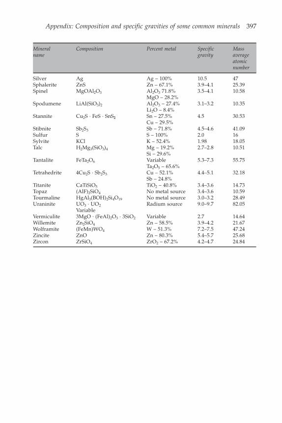
Appendix: Composition and specific gravities of some common minerals 397
Silver Ag Ag – 100% 10.5 47Sphalerite ZnS Zn – 67.1% 3.9–4.1 25.39Spinel MgOAl2O3 Al2O3 71.8% 3.5–4.1 10.58
MgO – 28.2%Spodumene LiAl(SiO3)2 Al2O3 – 27.4% 3.1–3.2 10.35
Li2O – 8.4%Stannite Cu2S · FeS · SnS2 Sn – 27.5% 4.5 30.53
Cu – 29.5%Stibnite Sb2S3 Sb – 71.8% 4.5–4.6 41.09Sulfur S S – 100% 2.0 16Sylvite KCl K – 52.4% 1.98 18.05Talc H2Mg3(SiO3)4 Mg – 19.2% 2.7–2.8 10.51
Si – 29.6%Tantalite FeTa2O6 Variable 5.3–7.3 55.75
Ta2O5 – 65.6%Tetrahedrite 4Cu2S · Sb2S3 Cu – 52.1% 4.4–5.1 32.18
Sb – 24.8%Titanite CaTiSiO5 TiO2 – 40.8% 3.4–3.6 14.73Topaz (AlF)2SiO4 No metal source 3.4–3.6 10.59Tourmaline HgAl3(BOH)2Si4O19 No metal source 3.0–3.2 28.49Uraninite UO3 · UO2 Radium source 9.0–9.7 82.05
VariableVermiculite 3MgO · (FeAl)2O3 · 3SiO2 Variable 2.7 14.64Willemite Zn2SiO4 Zn – 58.5% 3.9–4.2 21.67Wolframite (FeMn)WO4 W – 51.3% 7.2–7.5 47.24Zincite ZnO Zn – 80.3% 5.4–5.7 25.68Zircon ZrSiO4 ZrO2 – 67.2% 4.2–4.7 24.84
Mineral Composition Percent metal Specific Massname gravity average
atomicnumber

This Page Intentionally Left Blank
Index
Algorithms:direct substitution, 363for loop finding, 361for stream tearing, 361Newton–Raphson, 363
Andrews-Mika diagram, 58beta distribution model, 66boundaries of, 60discretized, 72for simulation, 385internal structure, 65
Apparent grade, 27, 49Attachment of particle to bubble, 294Attachment efficiency, 294, 309Attainable region, 60, 73Attrition test, JKMRC, 199Autogenous media separators, 243Autogenous mills:
attrition and wear in, 183, 198attrition test for, 199breakage functions in, 201breakage mechanisms in, 181effect of discharge grate in, 186population balance models for, 42, 181,
185self breakage in, 200specific rate of breakage in, 197
Batch milling, 205of heterogeneous solids, 208of homogeneous solids, 205
Baum jig, 266Beta distribution, 46
as model for Andrews-Mika diagrams,65
Bond work index, 151, 202efficiency factors for, 203
Breakage function, 136based on impact energy, 144based on truncated distributions, 143empirical, 139for multi-phase particles, 59in autogenous and semi-autogenous
mills, 201
in ball mills, 174in crushers, 159non-normalizedsingle particle, 136t10 model, 145
Breakage:boundary-region, 70differential, 70kinetics of, 172phase-boundary, 70preferential, 70selective, 97
Bubble rise times, 312Bubble Reynolds number, 295Bubble loading, 295, 305, 309Bubble surface in froth, variation along a
streamline, 330
Classification functions, 119exponential sum, 119logistic, 119Rosin-Rammler, 119sharpness index, 119
Classification, 81–125based on sieving, 81function, 86, 89hydrocyclone, 98
Coal washing plant, optimization, 372Coal washability, 379Collision angle, 300Collision efficiency, 294
measured for coal, 300measured for quartz, 300measurement of, 298model for, 297
Collisions between bubbles and particles,293
Comminution:energy requirements for, 150of multi-phase particles, 59
Critical speed, 164Crushers:
breakage function in, 159breakage zone in, 156

400 Index
capacities of, 161–163classification function in, 158cone, 154gyratory, 152jaw, 152open-side setting of, 153
Crushing, 152–163mechanisms, 155
Cut pointfor hydrocyclones, 114in dense media separators, 235optimum setting of, 374typical values in dense-media
separators, 240
Darcy’s Law, 227DEM simulations, 196Dense media separators, 234
cut point, 235density differential, 236imperfection, 237, 240partition curves for, 234, 239separation efficiency, 237short circuit flows in, 236short circuit flows, 238
Dense-medium cyclone, 235, 240Detachment efficiency, 294, 321Dewatering, 223–230
screens, 223Diamagnetic materials, 269, 271Differential breakage, 70Distribution:
by composition, 16by number, 32of collision angles, 301of induction times, 308
Distribution density, 13Distribution functions, 6
conditional, 19Gaudin-Meloy, 10Harris, 10joint, 17Log-normal, 8logarithmic, 10Logistic, 9plotting, 12Rosin-Rammler, 8truncated, 10, 143
Drag coefficient:for particles, 98for rising bubbles, 313
Drainage through plateau borders, 332,334
Drop weight test, 138Dry magnetic separation, 286–288
capacity, 286Hopstock model for, 283
Dynawhirlpool, 241
Energy:impact energy spectrum in mills, 195particle fracture energy, 132
EPM, factors for, 237, 265
Feeder region, 60, 73Filtercake, specific resistance, 228Filtration, 227–230
batch, 228Flotation, 289–350
bubble loading, 295bubblephase, 292distributed rate constant model for, 307,
339effect of particle size, 343entrained phase, 292froth phase, 292, 323–337kinetic model, 290, 293, 337models for continuous cells, 341pulp phase, 291simplified kinetic model, 337
Flowsheet structure, 355recycle loops in, 357
Fractureattrition and chipping, 130cleavage, 130Griffith theory, 134non-random, 69–72of brittle materials, 127particle fracture energy, 132random, 57shatter, 129toughness, 127
Froth transmission coefficient, 336Froth phase, 323–337
bubble residence time in, 332drainage in, 328film rupture in, 328
Crushers: (Contd)
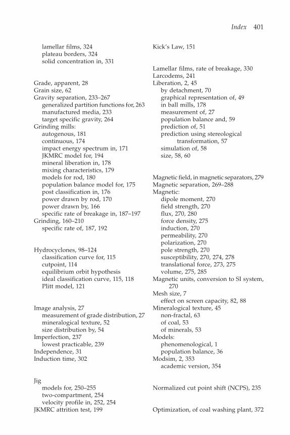
Index 401
lamellar films, 324plateau borders, 324solid concentration in, 331
Grade, apparent, 28Grain size, 62Gravity separation, 233–267
generalized partition functions for, 263manufactured media, 233target specific gravity, 264
Grinding mills:autogenous, 181continuous, 174impact energy spectrum in, 171JKMRC model for, 194mineral liberation in, 178mixing characteristics, 179models for rod, 180population balance model for, 175post classification in, 176power drawn by rod, 170power drawn by, 166specific rate of breakage in, 187–197
Grinding, 160–210specific rate of, 187, 192
Hydrocyclones, 98–124classification curve for, 115cutpoint, 114equilibrium orbit hypothesisideal classification curve, 115, 118Plitt model, 121
Image analysis, 27measurement of grade distribution, 27mineralogical texture, 52size distribution by, 54
Imperfection, 237lowest practicable, 239
Independence, 31Induction time, 302
Jigmodels for, 250–255two-compartment, 254velocity profile in, 252, 254
JKMRC attrition test, 199
Kick’s Law, 151
Lamellar films, rate of breakage, 330Larcodems, 241Liberation, 2, 45
by detachment, 70graphical representation of, 49in ball mills, 178measurement of, 27population balance and, 59prediction of, 51prediction using stereological
transformation, 57simulation of, 58size, 58, 60
Magnetic field, in magnetic separators, 279Magnetic separation, 269–288Magnetic:
dipole moment, 270field strength, 270flux, 270, 280force density, 275induction, 270permeability, 270polarization, 270pole strength, 270susceptibility, 270, 274, 278translational force, 273, 275volume, 275, 285
Magnetic units, conversion to SI system,270
Mesh size, 7effect on screen capacity, 82, 88
Mineralogical texture, 45non-fractal, 63of coal, 53of minerals, 53
Models:phenomenological, 1population balance, 36
Modsim, 2, 353academic version, 354
Normalized cut point shift (NCPS), 235
Optimization, of coal washing plant, 372
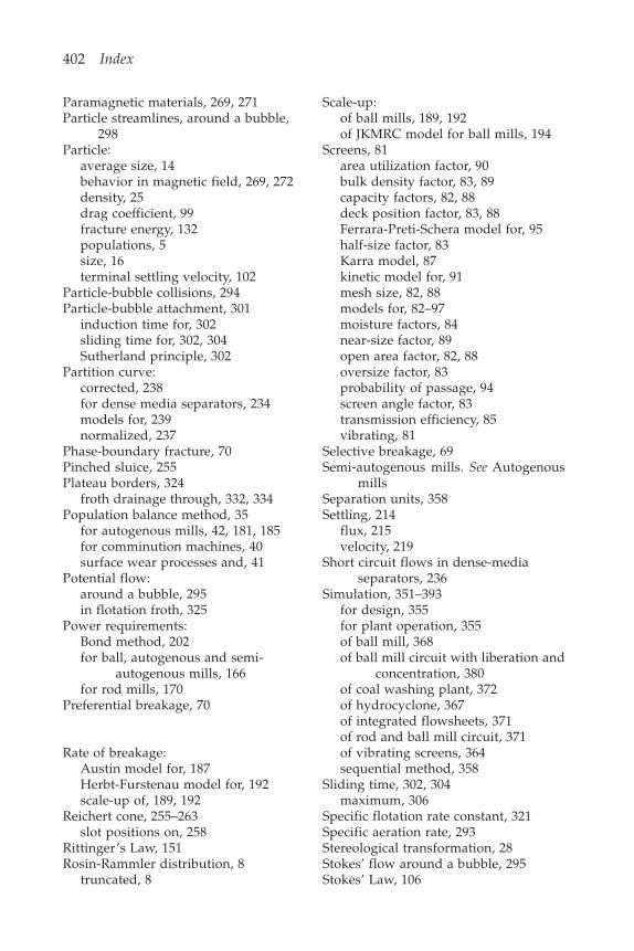
402 Index
Paramagnetic materials, 269, 271Particle streamlines, around a bubble,
298Particle:
average size, 14behavior in magnetic field, 269, 272density, 25drag coefficient, 99fracture energy, 132populations, 5size, 16terminal settling velocity, 102
Particle-bubble collisions, 294Particle-bubble attachment, 301
induction time for, 302sliding time for, 302, 304Sutherland principle, 302
Partition curve:corrected, 238for dense media separators, 234models for, 239normalized, 237
Phase-boundary fracture, 70Pinched sluice, 255Plateau borders, 324
froth drainage through, 332, 334Population balance method, 35
for autogenous mills, 42, 181, 185for comminution machines, 40surface wear processes and, 41
Potential flow:around a bubble, 295in flotation froth, 325
Power requirements:Bond method, 202for ball, autogenous and semi-
autogenous mills, 166for rod mills, 170
Preferential breakage, 70
Rate of breakage:Austin model for, 187Herbt-Furstenau model for, 192scale-up of, 189, 192
Reichert cone, 255–263slot positions on, 258
Rittinger’s Law, 151Rosin-Rammler distribution, 8
truncated, 8
Scale-up:of ball mills, 189, 192of JKMRC model for ball mills, 194
Screens, 81area utilization factor, 90bulk density factor, 83, 89capacity factors, 82, 88deck position factor, 83, 88Ferrara-Preti-Schera model for, 95half-size factor, 83Karra model, 87kinetic model for, 91mesh size, 82, 88models for, 82–97moisture factors, 84near-size factor, 89open area factor, 82, 88oversize factor, 83probability of passage, 94screen angle factor, 83transmission efficiency, 85vibrating, 81
Selective breakage, 69Semi-autogenous mills. See Autogenous
millsSeparation units, 358Settling, 214
flux, 215velocity, 219
Short circuit flows in dense-mediaseparators, 236
Simulation, 351–393for design, 355for plant operation, 355of ball mill, 368of ball mill circuit with liberation and
concentration, 380of coal washing plant, 372of hydrocyclone, 367of integrated flowsheets, 371of rod and ball mill circuit, 371of vibrating screens, 364sequential method, 358
Sliding time, 302, 304maximum, 306
Specific flotation rate constant, 321Specific aeration rate, 293Stereological transformation, 28Stokes’ flow around a bubble, 295Stokes’ Law, 106

Index 403
Stratification, 243density profile in, 247, 251in multi-component beds, 249in two-component system, 246Mayer principle, 243, 251on Reichert cone, 257potential energy for, 244quantitative model for, 244specific stratification constant, 245
Stream functionaround bubbles, 296for froth, 327for particles around bubbles, 298
Streamlinesaround a bubble, 295for drainage in froth, 333in froth phase, 325of particle around a bubble, 295
Sutherland principle, 302, 308
Terminal settling velocity, 102in flotation cell, 293, 298isolated sphere, 102–106isometric particles of arbitrary shape,
107Thickeners, 220–223
concentration profile in, 223design of, 221simulation of, 220
Thickening, 213continuous, 215discontinuities in, 217Kynch theory of, 213simulation, 220steady state, 218
Transformation units, 358
Ultimate recovery, 308, 339Unit operation, 356
Vorsyl separator, 241
Washability, 23data completion, 378
Water balance in flotation cell, 345Water-only cyclone, 265Weir, 323
height, 325Wet high intensity magnetic separation,
287

This Page Intentionally Left Blank


![23039871 Modeling and Simulation of Mineral Processing Systems[1]](https://static.fdocuments.net/doc/165x107/550242524a795971028b4ec6/23039871-modeling-and-simulation-of-mineral-processing-systems1.jpg)