2

Modeling and Simulation of High Performance Electrical Vehicle Powertrains in VHDL-AMS

K. Jaber, A. Fakhfakh and R. Neji National School of Engineers, Sfax

Tunisia

1. Introduction

Nowadays the air pollution and economical issues are the major driving forces in

developing electric vehicles (EVs). In recent years EVs and hybrid electric vehicles (HEVs)

are the only alternatives for a clean, efficient and environmentally friendly urban

transportation system (Jalalifar et al., 2007). The electric vehicle (EV) appears poised to make

a successful entrance to the personal vehicle mass market as a viable alternative to the

traditional internal combustion engine vehicles (ICE): Recent advances in battery technology

indicate decreasing production costs and increasing energy densities to levels soon

acceptable by broad consumer segments. Moreover, excluding the generation of the

electricity, EVs emit no greenhouse gases and could contribute to meeting the strict CO2

emission limits necessary to dampen the effect of global warming. Several countries around

the world have therefore initiated measures like consumer tax credits, research grants or

recharging station subsidies to support the introduction of the EV. Finally, the success

alternative vehicles like the Toyota Prius Hybrid proves a shift in consumer interest towards

cleaner cars with lower operating costs (Feller et al., 2009).

Nonetheless, the EV will first need to overcome significant barriers that might delay or even

prevent a successful mass market adoption. Permanent Magnet Synchronous Motor

(PMSM) is a good candidate for EVs.

In this work, a high level modelling and an optimization is reported for the determination of

time response (Tr) and power (P) of Electric Vehicle. The electric constant of back-

electromotive-force, stator d- and q- axes inductances, switching period, battery voltage,

stator resistance and torque gear ratio were selected as factors being able to influence Tr and

P. The optimization process was carried out with Doehlert experimental design (Jaber et al.,

2010).

The optimization is based on simulations of the chain of the electric vehicle; every block is

simulated with a different abstraction level using the hardware description language

VHDL-AMS. The chain of electric traction is shown in Figure 1. It consists of 4 components:

Control strategy, Inverter, PMSM model and Dynamic model. A right combination of these

four elements determines the performance of electric vehicles.

VHDL (Very High Speed Integrated Circuit Hardware Description Language) is a commonly used modelling language for specifying digital designs and event-driven systems. The popularity of VHDL prompted the development of Analog and Mixed-Signal

www.intechopen.com

Electric Vehicles – Modelling and Simulations

26

(AMS) extensions to the language and these extensions were standardized as IEEE VHDL-AMS in 1999. Some of the main features of this ASCII-based language include Model Portability, Analog and Mixed-Signal modeling, Conserved System and Signal Flow Modeling, Multi-domain modeling, Modeling at different levels of abstraction, and Analysis in time, frequency and quiescent domains. Since VHDL-AMS is an open IEEE standard, VHDL-AMS descriptions are simulator-independent and models are freely portable across tools. This not only prevents model designers from being locked in to a single tool or tool vendor but also allows a design to be verified on multiple platforms to ensure model fidelity.

Fig. 1. Model of traction chain

VHDL-AMS is a strict superset of VHDL and inherently includes language support for describing event-driven systems such as finite state machines. The standard not only provides language constructs for digital and analog designs but also specifies the interactions between the analogue and digital solvers for mixed-signal designs. The analog (continuous time) extensions allow the description of conserved energy systems (based on laws of conservation) as well as signal-flow models (based on block diagram modeling). VHDL-AMS distinguishes between the interface (ENTITY) of a model and its behavior (ARCHITECTURE). VHDL-AMS allows the association of multiple architectures with the same entity and this feature is typically used to describe a model at different levels of abstraction. With VHDL-AMS, it is possible to specify model behaviour for transient, frequency and quiescent domain simulations. Depending on the user’s choice of an analysis type, the appropriate behavior is simulated. The language is very flexible in that it allows different modeling approaches to be used, both individually and collectively. It is possible to describe model behavior with differential algebraic equations, value assignments and subprograms at a very abstract and mathematical level (McDermott et al., 2006). The VHDL-AMS language is an undiscovered asset for FPGA designers—a powerful tool to define and verify requirements in a non-digital context.

www.intechopen.com

Modeling and Simulation of High Performance Electrical Vehicle Powertrains in VHDL-AMS

27

As an electric vehicle is a multidisciplinary system, the new standard VHDL-AMS is suitable for the modelling and the simulation of such system in the same software environment and with different abstraction levels (Jaber et al., 2009).

2. Dynamic model

The first step in vehicle performance modelling is to write an electric force model. This is the force transmitted to the ground through the drive wheels, and propelling the vehicle forward. This force must overcome the road load and accelerate the vehicle (Sadeghi et al., 2009). For any mission profile, an electric road vehicle is subjected to forces that the onboard propulsion system has to overcome in order to propel or retard the vehicle. These forces are composed of several components as illustrated in Figure 2 .The effort to overcome these forces by transmitting power via the vehicle drive wheels and tyres to the ground is known as the total tractive effort or total tractive force.

Fig. 2. Forces on a vehicle

The rolling resistance is primarily due to the friction of the vehicle tires on the road and can be written as (Jalalifar et al., 2007):

RR V

f gMF = ´ ´ (1)

The aerodynamic drag is due to the friction of the body of vehicle moving through the air. The formula for this component is as in the following:

21

. . . .2DA x

SC VF = (2)

An other resistance force is applied when the vehicle is climbing of a grade. As a force in the opposite direction of the vehicle movement is applied:

.g.sinL vF M a= (3)

The power that the EV must develop at stabilized speed is expressed by the following equation:

( ).a RR DA LP V F F F= + + (4)

www.intechopen.com

Electric Vehicles – Modelling and Simulations

28

The power available in the wheels of the vehicle is expressed by:

. .V

P T rm em m Rwheels= (5)

According to the fundamental principle of dynamics the acceleration of the vehicle is given by:

P Pm a

M Vvg

-= (6)

. .( )

.em m wheels RR DA L

v wheels

T r R F F F

M R (7)

.( )l wheels RR DA LT R F F F (8)

.mm

wheels

r dW

R dt

g= (9)

A VHDL-AMS model for the dynamic model is specified in an “architecture” description as show in Listing 1.

ARCHITECTURE behav OF dynamic_model IS

QUANTITY Speedm_s : REAL := 0.0;

QUANTITY F_RR : REAL := 0.0;

QUANTITY F_DA : REAL := 0.0;

QUANTITY F_L : REAL := 0.0;

BEGIN

F_RR = = f*Mv*g;

F_DA = = 0.5*da*Sf*Cx* Speedm_s * Speedm_s;

F_L = = Mv*g*sin(alpha)

Tl = = Rwheels*( F_RR + F_DA + F_L);

Speedm_s 'dot = = (1.0/(Mv*Rwheels))*(rm*Tem-Tl);

Speedkm_h = = 3.6 * Speedm_s;

Wm = = (rm/Rwheels)*Speedm_s;

END ARCHITECTURE behav;

Listing 1. VHDL-AMS dynamic model

3. PMSM model

A permanent magnet synchronous motor (PMSM) has significant advantages, attracting the interest of researchers and industry for use in many applications.

www.intechopen.com

Modeling and Simulation of High Performance Electrical Vehicle Powertrains in VHDL-AMS

29

Usage of permanent magnet synchronous motors (PMSMs) as traction motors is common in electric or hybrid road vehicles (Dolecek et al., 2008). The dynamic model of the PMSM can be described in the d-q rotor frame as follows:

didV Ri L L i

d d d e q qdtw= + - (10)

didV Ri L L i K

q q q e d d mdtw w= + + + (11)

Where K Pmf= is the electric constant of back-electromotive-force (EMF), it is calculated

according to the geometrical magnitudes of the motor so that it can function with a high

speed. The equations giving the stator current can be written in the following form:

( )1

.I V L Id e q qd Ld s R

w= ++

(12)

( )1

.I V L I Kq e d d mq Lq s R

w w= - -+

(13)

The electromagnetic torque developed by the motor is given by the following equation:

3 1

2 2( ) e mT K I p L L I Iq d q d q (14)

The equation giving the angle by the motor can be written in the following form:

. m

dp W

dt

q= (15)

Figure 3 shows the description of the model of the PMSM in Simplorer 7.0 software.

Fig. 3. SIMPLORER model of the PMSM in the d-q rotor frame

www.intechopen.com

Electric Vehicles – Modelling and Simulations

30

4. Control strategy

In recent years, vector-controlled ac motors, such as induction motor, permanent-magnet synchronous motor (PMSM), and synchronous reluctance motor, have become standard in industrial drives and their performance improvement is an important issue. Particularly, improvement of control performance and drive efficiency is essentially required for drives used in electric vehicles (Ben Salah et al., 2008):

3

. sin( . ( ))2

T K I p tem s s

q q= - (16)

To achieve an optimal control, which means a maximum torque, it is necessary to satisfy the following condition:

. ( )2

p ts

pq q- = (17)

from where

I Is q= and 0I

d= (18)

d

q

roto

r mag

netic

axis

ps

2s p

a

sI

EMF

Fig. 4. Stator current and EMF in the d-q rotor frame

The first part (A) in figure 1 illustrates the control strategy. It presents a first PI speed control used for speed regulation. The output of the speed control is Iqref; its application to a second PI

current regulator makes the adjustment of phase and squaring currents. The outputs of current regulators are Vdref and Vqref; they are applied to a Park transformation block. Where, Vdref and Vqref are the forcing function to decide the currents in d-q axis model which may be obtained from 3-phase voltages (Va, Vb and Vc) through the park transformation technique as:

.cos( ) .sin( )a dref qrefV V Vq q= - (19)

2 2

.cos( ) .sin( )3 3

b dref qrefV V Vp p

q q= - - - (20)

4 4

.cos( ) .sin( )3 3

c dref qrefV V Vp p

q q= - - - (21)

www.intechopen.com

Modeling and Simulation of High Performance Electrical Vehicle Powertrains in VHDL-AMS

31

The generation of the control signals of the inverter is made by comparison of the simple tensions obtained following the regulation with a triangular signal. Its period is known as switching period. The different blocks constituting the traction chain were described in a VHDL-AMS structural model by including all expressions detailed above.

5. Inverter model

The structure of a typical three-phase VSI is shown in figure 6. As shown below, Va, Vb and Vc are the output voltages of the inverter. S1 through S6 are the six power transistors IGBT that shape the output, which are controlled by a, a’, b, b’, c and c’. When an upper transistor is switched on (i.e., when a, b or c are 1), the corresponding lower transistor is switched off (i.e., the corresponding a’, b’ or c’ is 0). The on and off states of the upper transistors, S1, S3 and S5, or equivalently, the state of a, b and c, are sufficient to evaluate the output voltage.

Fig. 5. Inverter connected to a balanced load

The relationship between the switching variable vector [a, b, c]t and the line-to-line output voltage vector [Vab Vbc Vca]t and the phase (line-to-neutral) output voltage vector [Va Vb Vc]t are given by the following relationships, where a, b, c are the orders of S1, S3, S5 respectively.

1 1 0

. 0 1 1 .

1 0 1

ab

bc

ca

a

E b

c

VVV

é ù é ù é ù-ê ú ê ú ê úê ú ê ú ê ú= -ê ú ê ú ê úê ú ê ú ê ú-ê ú ë û ë ûë û

2 1 11

. . 1 2 1 .3

1 1 2

a

b

c

a

E b

c

VVV

é ù é ù é ù- -ê ú ê ú ê úê ú ê ú ê ú= - -ê ú ê ú ê úê ú ê ú ê ú- -ê ú ë û ë ûë û

The different blocks constituting the traction chain were introduced both in MATLAB and SIMPLORER 7.0 softwares. They were described in structural models by including all expressions detailed above. The different simulation parameters are summarized in table 1:

www.intechopen.com

Electric Vehicles – Modelling and Simulations

32

Parameters Designation Values

Vmax Max Speed 80 km/h

Cx Drag coefficient of the vehicle 0.55

S Frontal surface of the vehicle 1.8 m2

f Coefficient of rolling friction 0.025

Mv Total mass of the vehicle 800 kg

p Pair of pole number 4

Table 1. Simulation parameters

6. Simulation results

6.1 MATLAB environment Figure 6 details the vector control (Id=0 strategy) of the vehicle, implemented under Matlab/simulink software.

Fig. 6. SIMULINK models for a vector control and his interaction in a chain of traction for vehicle

Figure 7 shows the simulation result. The reference speed of the EV is reached after 8.5s. Simulations with MATLAB are useful to verify that our system works well without any dysfunction. But in this case, the traction chain of the EV is described with ideal functional models. Going down in the hierarchical design level, more suitable software should be applied. For this reason, our system was described in VHDL-AMS and simulated with Simplorer 7.0 software.

www.intechopen.com

Modeling and Simulation of High Performance Electrical Vehicle Powertrains in VHDL-AMS

33

Fig. 7. Vehicle speed response in MATLAB/SIMULINK

6.2 VHDL-AMS virtual prototype VHDL-AMS descriptions were developed for each block of the electric vehicle including structural models. The obtained blocks were connected in Simplorer 7.0 Software environment to obtain a high level description our system as detailed on figure 8. The exposed blocks include analogue/digital electronic behavioural descriptions. It represents a so complex multi-domain system (Fakhfakh et al., 2006).

Fig. 8. Electric Vehicle description in Simplorer environment

6.3 Comparison The dynamic response of the vehicle speed is depicted in figure 9, obtained with both Simplorer and Matlab software. In table 2, we compare the simulation runtime and the obtained response time of the Electric Vehicle. We can distinguish clearly the difference between the two simulation results.

www.intechopen.com

Electric Vehicles – Modelling and Simulations

34

Fig. 9. Dynamic response of the vehicle speed in Simplorer and Matlab

Software Simulation runtime Time response of max speed

Matlab 24s 8.5 s

Simplorer 66s 6.5 s

Table 2. Simulation runtime simulation

To conclude, Matlab executes simulations more rapidly (24s); we obtained a dynamic response equal to 8.5s. Simplorer simulation runtime is three times longer due to the fact that the modelling abstraction level is lower compared to the functional description with Matlab; the dynamic response is about 6.5s. The power of the Electric Vehicule is about 42 kW. To resume, we can clearly conclude that simulating a mathematical model with MATLAB software is useful to verify the ideal response of our EV. But with Simplorer environment we can attend the lower abstraction models. In this case, it is possible to simulate the effect of physical parameters such as temperature, battery voltage, etc.

7. Optimization with experimental designs

To optimize our control strategy, we have adopted an experimental design approach by

applying the Doehlert design. Six factors have been considered as shown on table 3: Ke, Ld,

Ts, E, R and rm. According to the number of factors, in order to limit the number of runs

and to take into account the major effects, a screening study is necessary. Consequently, a

first step of screening was conducted using a fractional factorial design. The last with six

factors is a design involving a minimum of 45 experiments (see appendix).

For each factor, we define three levels: low, center and high levels as detailed on table 3.

Naturel Variable

Parameters Coded

variable Low Level

Center Level

High Level

Ke electric constant of back-

electromotive-force (EMF) X1 0.05 0.1 0.2

Ld= Lq Stator d- and q- axes inductances (mH).

X2 0.216 0.416 0.616

Ts Switching period (s) X3 100 300 500

E Battery voltage (V) X4 200 300 400

R Stator resistance (Ω) X5 0.02 0.05 0.08

rm Torque gear ratio X6 1 3 5

Table 3. Description of experimental variables in the screening design

Speed (Km/h) Ref Speed Speed (Simplorer) Speed (Matlab)

www.intechopen.com

Modeling and Simulation of High Performance Electrical Vehicle Powertrains in VHDL-AMS

35

Our goal is to optimize both the response time and the power of the studied system. The analysis of results and the building of experimental designs were carried out with the NEMRODW mathematical statistical software (El Ati-Hellal et al., 2009). Because of the none-linearity of the studied system, the experimental response Yi can be represented by a quadratic equation of the response surface (Elek et al., 2004):

6 6

1,2 0 112

i i ij i jiiji j

Y b b x b x x===¹

= + +å å (19)

Y1 : response representing the response time; Y2 : response representing the power; To find an optimum, we should minimize (Y1) and maximize (Y2). So we define the following experimental response Y:

21

.Y YY

ab= + with =350 and =0.6 (20)

and are ponderation factors. In our case, we give the same weight to the response time and the power. Coefficients bi of the response surface (19) were calculated with Nemrodw software without taking into account experiment 45 due to high residual. To decide about the efficiency of the obtained regression equation, we compute R2 as: R2 = (Sum of squares attributed to the regression)/ Total Sum of squares) We found R² = 0.976; it is well within acceptable limits of R2>= 0.8 which revealed that the experimental data well fitted the second-order polynomial equation as detailed on table 4.

Y

Standard error of response 8.4837

R2 0.976 R2A 0.939 R2 pred 0.777 PRESS 11512.167 Degrees of freedom 17

Table 4. Statiscal data and coefficients of y response model: y= f(x1, x2, x3, x4, x5, x6)

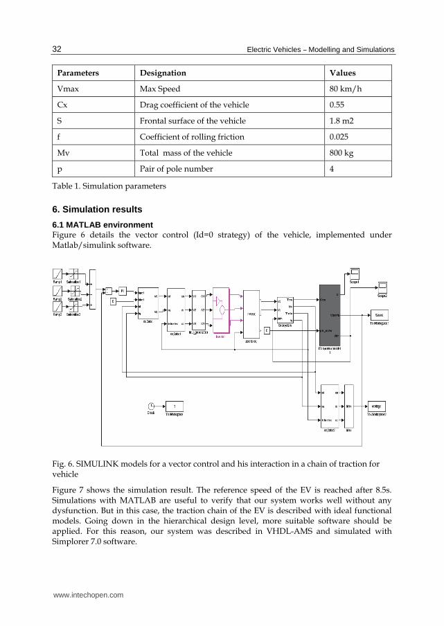
To estimate the quality of the model and validate it, analysis of the variance and the residual

values (difference between the calculated and the experimental result) were examined.

According to the residual (Figure 10), the choice of the model was appropriate: a systematic

behavior was not observed in the plot, for example, an increase in residual suggesting the

necessity to transform the response.

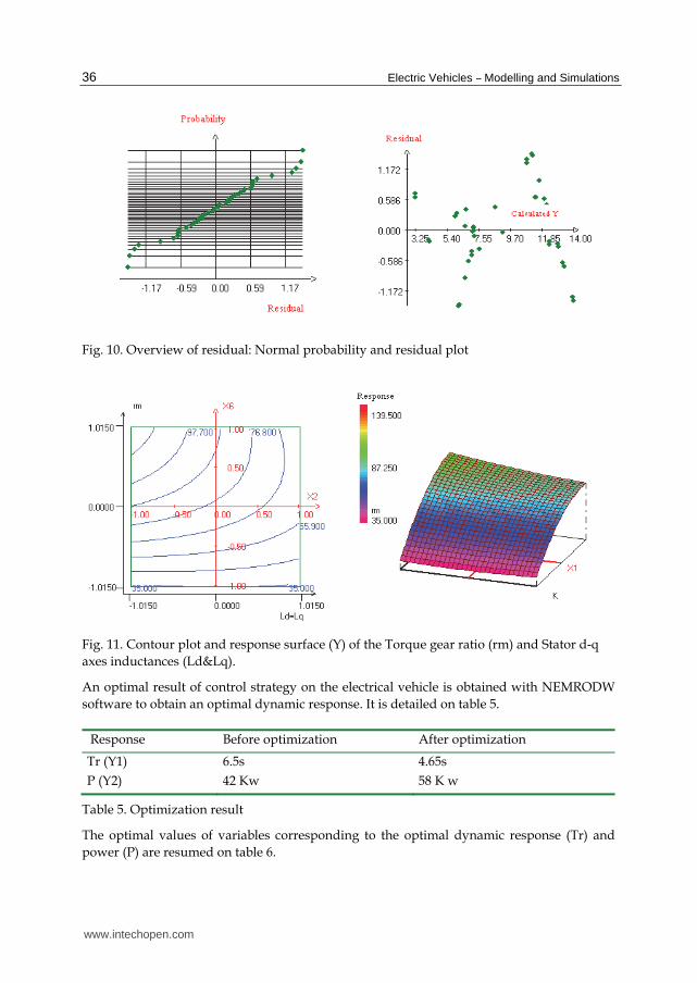
After the validation of the proposed second-order polynomial model, we can draw 2D and 3D

plots representing the evolution of Y versus 2 factors.

Using contour plot graphs makes the evaluation of the influences of the selected factors easier.

Figure 11 illustrates the experimental response obtained by the simultaneous variation of X2

(Ld&Lq) and X6 (rm). We concluded that in order to increase the response Y, an increase of

X6 and decrease of X2 is necessary (Danion et al., 2004) & (El Hajjaji et al., 2005).

www.intechopen.com

Electric Vehicles – Modelling and Simulations

36

Fig. 10. Overview of residual: Normal probability and residual plot

Fig. 11. Contour plot and response surface (Y) of the Torque gear ratio (rm) and Stator d-q

axes inductances (Ld&Lq).

An optimal result of control strategy on the electrical vehicle is obtained with NEMRODW

software to obtain an optimal dynamic response. It is detailed on table 5.

Response Before optimization After optimization

Tr (Y1) 6.5s 4.65s

P (Y2) 42 Kw 58 K w

Table 5. Optimization result

The optimal values of variables corresponding to the optimal dynamic response (Tr) and

power (P) are resumed on table 6.

www.intechopen.com

Modeling and Simulation of High Performance Electrical Vehicle Powertrains in VHDL-AMS

37

Variable Factor Optimal value in NEMRODW

Real values before optimization

Real values after optimization

X1 K 1.0094 0.1 0.2

X2 Ld=Lq 0.3976 0.416 mH 0.216 mH

X3 Ts 1.0086 300 s 500 s

X4 E 1.0052 300 V 400 V

X5 R 1.0061 0.05 Ω 0.08 Ω

X6 rm 0.9934 3 5

Table 6. Optimal values of variables

The speed response shows the good dynamic suggested of our vehicle. The reference speed is attained in 4.65 second. The direct current is equal to zero in the permanent mode, the quadratic current present the image of the electromagnetic torque. The power is increased to reach 58 kW.

0

100.00

50.00

0 18.001.00 3.00 5.00 7.00 9.00 11.00 13.00 15.00

Speed

SUM1.VAL dynamic_model...

Fig. 10. Dynamic response of the vehicle speed after optimization

10. Conclusion

In this paper, we developed a VHDL-AMS description of a vehicle traction chain and we adopt the vector control Id=0 strategy to drive the designed PMSM. The simulation of the dynamic response of the vehicle shows the effectiveness of this mode of control and the PMSM in the field of the electric traction. The obtained result with Simplorer differs from that obtained with Matlab because we used more accurate models. We think that VHDL-AMS is more suitable to predict the electric vehicle behavior since it is a multidisciplinary HDL. We have shown that response surface analysis coupled with a carefully constructed experimental design is a useful tool to carry out an Optimal Simulation of the Control Strategy of an Electrical Vehicle.

11. Nomenclature

Vd, Vq Stator d- and q- axes voltages (V).

id, iq Stator d- and q- axes currents (A).

www.intechopen.com

Electric Vehicles – Modelling and Simulations

38

R Stator resistance (Ω).

Ld,Lq Stator d- and q- axes inductances (H).

p Number of poles pairs.

Øm Flux created by rotor magnets (Wb).

wm Angular speed of the motor (rad/s).

f Coefficient of rolling friction.

Mv Total mass of the vehicle (kg).

g Acceleration of terrestrial gravity (m/s2).

l Density of the air (kg/m3).

S Frontal surface of the vehicle (m2).

Cx Drag coefficient of the vehicle.

V Speed of vehicle (m/s).

α Angle that make the road with the horizontal (in °).

rm Torque gear ratio.

Rwheels Wheels radius (m).

Tem Electromagnetic torque of the motor (N.m)

γ Acceleration of the vehicle (s-2).

Tl Load torque (N.m).

E Battery voltage

Ts Switching period

Vmax Maximum speed

12. Appendix – Doehlert matrix (six factors)

N°Exp

Factors Responses Y=/Y1+Y2

Ke Ld=Lq [mH]

Ts [µs]

E [V] R [ohm]

rm Y1(Tr)

[s] Y2(P) [Kw]

Response (Y)

1 -1 -1 -1 -1 -1 -1 12.62 13.08 35.582 2 1 -1 -1 -1 -1 1 12.10 52.80 60.600 3 -1 1 -1 -1 -1 1 12.08 20.00 40.973 4 1 1 -1 -1 -1 -1 12.64 12.78 35.358 5 -1 -1 1 -1 -1 1 4.80 58.00 107.710 6 1 -1 1 -1 -1 -1 12.67 12.72 35.256 7 -1 1 1 -1 -1 -1 12.63 12.85 35.422 8 1 1 1 -1. -1 1 12.09 24.70 43.770 9 -1 -1 -1 1 -1 1 3.89 100.00 149.974 10 1 -1 -1 1 -1 -1 12.63 12.50 35.212 11 -1 1 -1 1 -1 -1 12.64 13.00 35.490 12 1 1 -1 1 -1 1 6.60 39.86 76.946 13 -1 -1 1 1 -1 -1 12.64 12.80 35.370

www.intechopen.com

Modeling and Simulation of High Performance Electrical Vehicle Powertrains in VHDL-AMS

39

14 1 -1 1 1 -1 1 4.00 98.00 146.300 15 -1 1 1 1 -1 1 6.40 40.00 78.687 16 1 1 1 1 -1 -1 12.64 12.68 35.298 17 -1 -1 -1 -1 1 1 4.71 60.00 110.310 18 1 -1 -1 -1 1 -1 12.66 12.24 35.000 19 -1 1 -1 -1 1 -1 12.66 12.28 35.014 20 1 1 -1 -1 1 1 12.15 20.00 40.806 21 -1 -1 1 -1 1 -1 12.65 12.27 35.030 22 1 -1 1 -1 1 1 12.16 50.00 58.783 23 -1 1 1 -1 1 1 12.02 21.00 41.720 24 1 1 1 -1 1 -1 12.65 12.27 35.030 25 -1 -1 -1 1 1 -1 12.66 12.90 35.386 26 1 -1 -1 1 1 1 4.00 96.80 145.580 27 -1 1 -1 1 1 1 6.24 40.00 80.090 28 1 1 -1 1 1 -1 12.64 12.34 39.094 29 -1 -1 1 1 1 1 3.96 101.00 148.983 30 1 -1 1 1 1 -1 12.65 12.36 35.084 31 -1 1 1 1 1 -1 12.64 12.47 35.172 32 1 1 1 1 1 1 6.28 40.40 79.972 33 -1 0 0 0 0 0 7.11 46.18 76.934 34 1 0 0 0 0 0 7.26 44.77 75.071 35 0 -1 0 0 0 0 6.71 60.40 88.401 36 0 1 0 0 0 0 9.12 31.00 57.000 37 0 0 -1 0 0 0 7.24 45.15 75.432 38 0 0 1 0 0 0 7.18 45.30 76.000 39 0 0 0 -1 0 0 9.14 30.55 56.623 40 0 0 0 1 0 0 6.72 58.37 87.105 41 0 0 0 0 -1 0 7.24 45.50 75.642 42 0 0 0 0 1 0 7.13 46.39 77.000 43 0 0 0 0 0 -1 12.65 12.55 35.198 44 0 0 0 0 0 1 5.73 46.70 89.102

45 0 0 0 0 0 0 7.16 46.00 76.480

13. References

Jalalifar, M.; Payam, A. F.; Nezhad, S. & Moghbeli, H. (2007). Dynamic Modeling and Simulation of an Induction Motor with Adaptive Backstepping Design of an Input-Output Feedback Linearization Controller in Series Hybrid Electric Vehicle, Serbian Journal of Electrical Engineering, Vol.4, No.2, (November 2007), pp. 119-132.

Feller, A. & Stephan, M. (2009). Modeling Germany＇s Transition to the EV until 2040 in

System Dynamics, Thesis, Vallendar, July 27, 2009. Jaber, K.; Fakhfakh , A. & Neji, R. (2010). High Level Optimization of Electric Vehicle Power-

Train with Doehlert Experimental Design, 11 th International Workshop on Symbolic and Numerical Methods, Modeling and Apllications to Circuit Design, Sm2ACD 2010, pp. 908-911, ISBN 978-1-4244-5090-9, Tunis-Gammarth, Tunisia, 2010.

www.intechopen.com

Electric Vehicles – Modelling and Simulations

40

Jaber, K.; Ben Saleh, B.; Fakhfakh , A. & Neji, R. (2009). Modeling and Simulation of electrical vehicle in VHDL-AMS, 16 th IEEE International Conference on, Electonics, Circuits, and Systems, ICECS 2009, pp. 908-911, ISBN 978-1-4244-5090-9, Yasmine Hammamet, Tunisia, 2009.

McDermott, T. E.; Juchem, R. & Devarajan, D. (2006). Distribution Feeder and Induction Motor Modeling with VHDL-AMS. 2006 IEEE/PES T&D Conference and Exposition Proceedings, 21-26 May 2006, Dallas.

Fakhfakh, A., Feki, S., Hervé, Y., Walha, A. & Masmoudi, N., Virtual prototyping in power electronics using VHDL-AMS application to the direct torque control optimisation, J. Appl. Sci. 6, 2006, pp. 572-579.

Sadeghi, S. & Mirsalim, M. (2010). Dynamic Modeling and Simulation of a Switched Reluctance Motor in a Series Hybrid Electric Vehicle, International peer-reviewed scientific journal of Applied sciences, Vol.7, No.1, (2010), pp. 51-71, ISBN 1785-8860.

Dolecek, R.; Novak, J. & Cerny, O. (2009). Traction Permanent Magnet Synchronous Motor Torque Control with Flux Weakening. Radioengineering, VOL. 18, NO. 4, DECEMBER 2009.

Ben Salah, B.; Moalla, A.; Tounsi, S.; Neji, R. & Sellami, F. (2008). Analytic Design of a Permanent Magnet Synchronous Motor Dedicated to EV Traction with a Wide Range of Speed Operation, International Review of Electrical Engineering (I.R.E.E.), Vol.3, No.1, (2008), pp. 110-12.

El Ati-Hellal, M.; Hellal , F.; Dachraoui, M. & Hedhili, A. (2009). Optimization of Sn determination in macroalgae by microwaves digestion and transversely heated furnace atomic absorption spectrometry analysis. Canadian Journal of Analytical Sciences and Spectroscopy, Vol.53, No.6, 2009.

Elek, J.; Mangelings, D.; Joó, F. & V. Heyden, Y. (2004). Chemometric modelling of the catalytic Hydrogenation of bicarbonate to formate in aqueous Media, Reaction Kinetics and Catalysis Letters. Vol.83, No.2, (2004), pp. 321-328.

Danion, A.; Bordes, C.; Disdier, J.; Gauvrit, J.Y.; Guillard, C.; Lantéri, P. & Renault, N. J. (2004). Optimization of a single TiO2-coated optical fiber reactor using experimental design, Elsevier, Journal of Photochemistry and Photobiology A: Chemistry , Vol.168 , No.3, (2004), pp. 161-167.

El Hajjaji, S.; El Alaoui, M.; Simon, P.; Guenbour, A.; Ben Bachir, A.; Puech-Costes, E.; Maurette, M.-T. & Aries, L. (2005). Preparation and characterization of electrolytic alumina deposit on austenitic stainless steel. Science and Technology of Advanced Materials, Vol.6, No.5, (2005), pp. 519-524, ISSN 1468-6996.

www.intechopen.com

Electric Vehicles - Modelling and SimulationsEdited by Dr. Seref Soylu

ISBN 978-953-307-477-1Hard cover, 466 pagesPublisher InTechPublished online 12, September, 2011Published in print edition September, 2011

InTech EuropeUniversity Campus STeP Ri Slavka Krautzeka 83/A 51000 Rijeka, Croatia Phone: +385 (51) 770 447 Fax: +385 (51) 686 166www.intechopen.com

InTech ChinaUnit 405, Office Block, Hotel Equatorial Shanghai No.65, Yan An Road (West), Shanghai, 200040, China

Phone: +86-21-62489820 Fax: +86-21-62489821

In this book, modeling and simulation of electric vehicles and their components have been emphasizedchapter by chapter with valuable contribution of many researchers who work on both technical and regulatorysides of the field. Mathematical models for electrical vehicles and their components were introduced andmerged together to make this book a guide for industry, academia and policy makers.

How to referenceIn order to correctly reference this scholarly work, feel free to copy and paste the following:

K. Jaber, A. Fakhfakh and R. Neji (2011). Modeling and Simulation of High Performance Electrical VehiclePowertrains in VHDL-AMS, Electric Vehicles - Modelling and Simulations, Dr. Seref Soylu (Ed.), ISBN: 978-953-307-477-1, InTech, Available from: http://www.intechopen.com/books/electric-vehicles-modelling-and-simulations/modeling-and-simulation-of-high-performance-electrical-vehicle-powertrains-in-vhdl-ams