Modeling and Simulation of an All Electric Ship

Modeling and Simulation of an All Electric Ship

in Random SeasMASSACHUSETTS INSTITUTE

by OF TECHNOLOGYbyO

Kyle Schmitt NOV 0 4 2010

B.S., University of Wisconsin - Madison (2008) LBRARIES

Submitted to the Department of Mechanical Engineering ARCHIVESin partial fulfillment of the requirements for the degree of

Master of Science in Mechanical Engineering

at the

MASSACHUSETTS INSTITUTE OF TECHNOLOGY

September 2010

© Massachusetts Institute of Technology 2010. All rights reserved.

I,}Author .. . . . ... *. .V. . r . . . . . . . . . .

Department of Mechanical EngineeringAugust 13, 2010

C ertified by ..................... ... .... . ...............

Michael TriantafyllouWilliam I. Koch Professor of Marine Technology

Thesis Supervisor

'A -n

A ccep ted by ............................. . ............................David E. Hardt

Chairman, Committee on Graduate Students

- -- amow

Modeling and Simulation of an All Electric Ship

in Random Seas

by

Kyle Schmitt

Submitted to the Department of Mechanical Engineeringon August 13, 2010, in partial fulfillment of the

requirements for the degree ofMaster of Science in Mechanical Engineering

Abstract

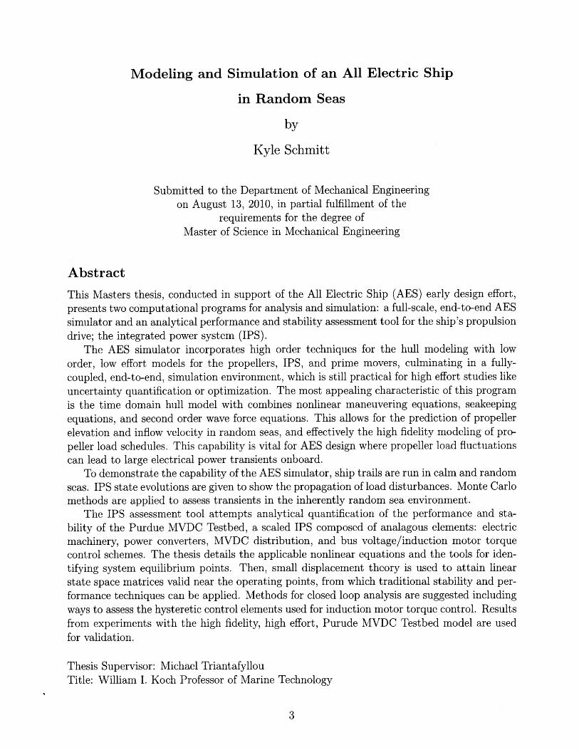
This Masters thesis, conducted in support of the All Electric Ship (AES) early design effort,presents two computational programs for analysis and simulation: a full-scale, end-to-end AESsimulator and an analytical performance and stability assessment tool for the ship's propulsiondrive; the integrated power system (IPS).

The AES simulator incorporates high order techniques for the hull modeling with loworder, low effort models for the propellers, IPS, and prime movers, culminating in a fully-coupled, end-to-end, simulation environment, which is still practical for high effort studies likeuncertainty quantification or optimization. The most appealing characteristic of this programis the time domain hull model with combines nonlinear maneuvering equations, seakeepingequations, and second order wave force equations. This allows for the prediction of propellerelevation and inflow velocity in random seas, and effectively the high fidelity modeling of pro-peller load schedules. This capability is vital for AES design where propeller load fluctuationscan lead to large electrical power transients onboard.

To demonstrate the capability of the AES simulator, ship trails are run in calm and randomseas. IPS state evolutions are given to show the propagation of load disturbances. Monte Carlomethods are applied to assess transients in the inherently random sea environment.

The IPS assessment tool attempts analytical quantification of the performance and sta-bility of the Purdue MVDC Testbed, a scaled IPS composed of analagous elements: electricmachinery, power converters, MVDC distribution, and bus voltage/induction motor torquecontrol schemes. The thesis details the applicable nonlinear equations and the tools for iden-tifying system equilibrium points. Then, small displacement theory is used to attain linearstate space matrices valid near the operating points, from which traditional stability and per-formance techniques can be applied. Methods for closed loop analysis are suggested includingways to assess the hysteretic control elements used for induction motor torque control. Resultsfrom experiments with the high fidelity, high effort, Purude MVDC Testbed model are usedfor validation.

Thesis Supervisor: Michael TriantafyllouTitle: William I. Koch Professor of Marine Technology

Acknowledgments

My plenary acknowledgement and expression of thanks go to the MIT faculty and Sea Grant

staff for investing in my work without question. I was truly blown away by the readiness of

my superiors to aid in my endeavors. No matter the department, no matter the query, MIT

faculty and staff were willing to address my needs duly and unfailingly. In specific, I would like

to thank Michael Triantafyllou, Franz Hover, James Kirtley, Chryssostomos Chryssostomidis,

Mirjana Marden, George Karniadakis, Julie Chalfant, Mark Welsh, and Trent Gooding for

their technical guidance.

From an administration standpoint, I'd like to thank Michael Triantafyllou, Chryssostomos

Chryssostomidis, and Franz Hover for keeping me on task and motivating new avenues for self-

education and research. Prof. Triantafyllou and Chrys, without your immense patience and

resolve, I could not have produced the work to follow. Prof. Hover, without your unique

perspective, I could not have garnered nearly the same intellectual experience from my time

at MIT.

Both in my lab group and outside of it, I am indebted to several MIT students for moral and

technical support. I'd like to give special recognition to Brenden Englot for always allowing

me to verbalize my ideas on a near daily basis and for supplementing them with his experience.

I'd also like Ilkay Erselscan for his infinite patience, help, and kindness during the development

of my seakeeping model. Additional recognition needs to be given to Charlie Ambler, Brendon

Epps, Josh Taylor, Phil Menard, Steve Englebretson, Lynn Sarcione, and Kevin Cedrone.

Thank you to the Office of Naval Research for providing the financial means that fueled

this thesis.

Finally, thank you to my parents Patrick and Peggy Schmitt for building on an already

significant debt of gratitude. Without your unyielding support, I would not be the student,

engineer, person, that I am today.

Contents

1 Introduction1.1 An Historical Introduction to the All Electric Ship.

1.1.1 Advantages and Challenges . . . . . . . . . .1.2 Current Focus Areas for AES Research . . . . . . . .1.3 Thesis Deliverables . . . . . . . . . . . . . . . . . . .

1.3.1 AES Simulator . . . . . . . . . . . . . . . . .1.3.2 Performance and Stability Analysis of the IPS

1.4 Outline of Thesis . . . . . . . . . . . . . . . . . . . .

2 An End-to-End Model of the AES2.1 Gas Turbine Model . . . . . . . . . . .2.2 IPS M odel . . . . . . . . . . . . . . . .

2.2.1 Synchronous Machine . . . . . .2.2.2 Induction Motor . . . . . . . .2.2.3 Rectification, Transmission, and2.2.4 Volts per Hertz IM Control . .

2.3 Propeller and Surge Model . . . . . . .2.4 Nonlinear Maneuvering Model . . . . .

2.4.1 Rudder Model . . . . . . . . . .2.5 Time Domain Seakeeping Model . . . .

2.5.1 Conformal Mapping . . . . . .2.5.2 Strip Theory . . . . . . . . . .2.5.3 Second Order Forces . . . . . .2.5.4 Time Domain Generalization .

Inversion Models

3 High Fidelity Component Model Alternatives3.1 A LQG-LTR Controlled Jet Turbine Model . . .

3.1.1 Development of LQG-LTR Controller . .3.1.2 Numerical Results Comparison3.1.3 From Jet Turbine Model to Electrical Generation Model

3.2 Advanced Propeller Modeling Techniques . . . . . . . . . . . . .3.2.1 Vortex Lattice Line Method . . . . . . . . . . . . . . . .3.2.2 Modern Cavitation Methods . . . . . . . . . . . . . . . .

11. . . . . . . . . . . . 1 1. . . . . . . . . . . . 14. . . . . . . . . . . . 15. . . . . . . . . . . . 17. . . . . . . . . . . . 18. . . . . . . . . . . . 19. . . . . . . . . . . . 19

212123242527293032373941424547

52. . . . . . 53. . . . . . 54. . . . . . 57. . . . . . 60. . . . . . 61. . . . . . 61. . . . . . 62

. . . . . . . . . . . . . . ..

.

.

4 Stability Analysis of the MVDC Integrated Power System4.1 Description of IPS Models ....... ............................. 65

4.1.1 Generator Side Models . . . . . . . . . . . . . . . . . . . . . . . . . . . 664.1.2 Motor Side Models . . . . . . . . . . . . . . . . . . . . . . . . . . . . . 71

4.2 Steady State Linearization . . . . . . . . . . . . . . . . . . . . . . . . . . . . . 764.2.1 Generator Side Linearization . . . . . . . . . . . . . . . . . . . . . . . . 764.2.2 Motor Side Linearization . . . . . . . . . . . . . . . . . . . . . . . . . . 81

4.3 Open Loop Analysis . . . . . . . . . . . . . . . . . . . . . . . . . . . . . . . . 854.3.1 Generator Side Open Loop Analysis . . . . . . . . . . . . . . . . . . . . 854.3.2 Motor Side Open Loop Analysis . . . . . . . . . . . . . . . . . . . . . . 87

4.4 Closed Loop Analysis . . . . . . . . . . . . . . . . . . . . . . . . . . . . . . . . 894.4.1 Generator Side Closed Loop Analysis . . . . . . . . . . . . . . . . . . . 894.4.2 Motor Side Closed Loop Analysis . . . . . . . . . . . . . . . . . . . . . 90

5 Simulation Results with AES Model 955.1 Conservation of Power across IPS . . . . . . . . . . . . . . . . . . . . . . . . . 965.2 IPS Performance during Routine Maneuvering . . . . . . . . . . . . . . . . . . 98

5.2.1 A cceleration . . . . . . . . . . . . . . . . . . . . . . . . . . . . . . . . . 995.2.2 A C Braking . . . . . . . . . . . . . . . . . . . . . . . . . . . . . . . . . 1005.2.3 Heading Changes . . . . . . . . . . . . . . . . . . . . . . . . . . . . . . 1035.2.4 Second Order Forces . . . . . . . . . . . . . . . . . . . . . . . . . . . . 103

5.3 IPS Performance in Random Sea Environments . . . . . . . . . . . . . . . . . 1055.3.1 Seakeeping in Head Seas . . . . . . . . . . . . . . . . . . . . . . . . . . 1065.3.2 Seakeeping during 360 Degree Maneuver . . . . . . . . . . . . . . . . . 106

5.4 Stochastic Simulation with AES Simulator . . . . . . . . . . . . . . . . . . . . 1085.4.1 Statistics of High Frequency Surface Effects . . . . . . . . . . . . . . . 1105.4.2 Statistics of Low Frequency Surface Effects . . . . . . . . . . . . . . . . 112

6 Conclusions and Future Research6.1 Recommended Research and Studies

116117

64

List of Figures

1-1 Recent past and near future composition of the surface combatant force [63]. 131-2 Thermal efficiency vs. size for several options of propulsion power [66]. .... 141-3 Current focus areas in AES development. The asterisks designate areas of

research directly related to the work presented in this Master's thesis. . . . . . 16

2-1 A schematic of the AES model presented in this thesis. . . . . . . . . . . . . . 222-2 Equivalent circuit (SM ). . . . . . . . . . . . . . . . . . . . . . . . . . . . . . . 242-3 Equivalent Circuit (IM ). . . . . . . . . . . . . . . . . . . . . . . . . . . . . . . 252-4 Operation curves for a notional 38 MW IM with volts per Hertz control. . . . 262-5 Traditional three phase rectifier-inverter [52]. . . . . . . . . . . . . . . . . . . . 272-6 Schematic of lower order rectifier-inverter model . . . . . . . . . . . . . . . . . 282-7 Volts per Hertz control protocol. . . . . . . . . . . . . . . . . . . . . . . . . . . 302-8 Demonstration of propeller loss model. . . . . . . . . . . . . . . . . . . . . . . 322-9 Body-fixed and earth-fixed reference frames [23]. . . . . . . . . . . . . . . . . . 332-10 Beam comparison between DDG51 hull and Chesapeake Pro kayak. . . . . . . 372-11 Rudder schem atic. . . . . . . . . . . . . . . . . . . . . . . . . . . . . . . . . . 382-12 Non-dimensional sectional added mass and damping in sway direction for a

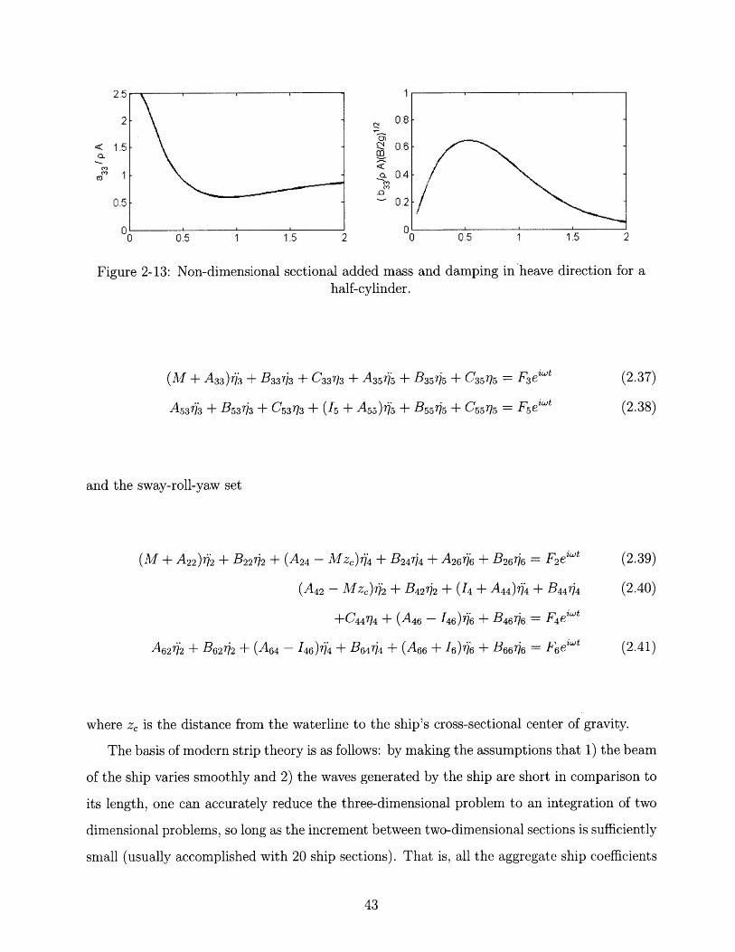
half-cylinder. . . . . . . . . . . . . . . . . . . . . . . . . . . . . . . . . . . . . 422-13 Non-dimensional sectional added mass and damping in heave direction for a

half-cylinder. . . . . . . . . . . . . . . . . . . . . . . . . . . . . . . . . . . . . 432-14 RAOs for half-cylinder in heave and pitch. . . . . . . . . . . . . . . . . . . . . 452-15 RAOs for half-cylinder in sway, roll, and yaw. . . . . . . . . . . . . . . . . . . 462-16 Second order force result comparison with [61]. . . . . . . . . . . . . . . . . . . 472-17 Bretschneider spectrums for different sea states. . . . . . . . . . . . . . . . . . 50

3-1 Closed loop schematic for LQG-LTR controlled F-100. . . . . . . . . . . . . . 543-2 Singular value plot for Kalman loop transfer function after loopshaping. . . . . 563-3 Singular values for Kappos' open and closed loop transfer functions. . . . . . . 573-4 Singular values for this thesis's open and closed loop transfer functions. . . . . 583-5 Input screen for OpenProp2.2. . . . . . . . . . . . . . . . . . . . . . . . . . . . 62

4-1 A schematic of the Purdue MVDC Testbed [49]. . . . . . . . . . . . . . . . . . 644-2 Turbine-Generator side process flow diagram. . . . . . . . . . . . . . . . . . . 664-3 DC bus voltage droop control [49]. . . . . . . . . . . . . . . . . . . . . . . . . 714-4 Motor-Propeller side process flow diagram. . . . . . . . . . . . . . . . . . . . . 714-5 Torque trim controller [49] . . . . . . . . . . . . . . . . . . . . . . . . . . . . . 74

4-6 Dynamics of current hysteresis control for a phase: a) Resulting induction motorcurrent for a single phase and b) the stator voltage for the same phase. .... 76

4-7 Bode plot for the generator side with field voltage input and droop feedbackoutput for baseline operating conditions, T* = 100 Nm. Stars indicate highfidelity simulation results. . . . . . . . . . . . . . . . . . . . . . . . . . . . . . 86

4-8 Bode plot for motor-propeller with stator voltage input and stator current mag-nitude feedback for the output, for a 100 Nm operating condition. Stars indicatePurdue MVDC Testbed model results. . . . . . . . . . . . . . . . . . . . . . . 89

4-9 Bode plot for motor-propeller with stator voltage input and stator current mag-nitude feedback for the output, for a 200 Nm operating condition. Stars starsindicate Purdue MVDC Testbed model results. . . . . . . . . . . . . . . . . . 90

4-10 Three phase hysteresis current control for IM torque management. . . . . . . . 914-11 A generalized combined phase hysteresis control. . . . . . . . . . . . . . . . . . 914-12 Bode plot for closed loop motor-propeller system using instantaneous voltage

assumption, for T,*, =100 Nm. . . . . . . . . . . . . . . . . . . . . . . . . . . . 94

5-1 Time evolution of propeller speed and ship speed for startup. . . . . . . . . . . 975-2 Power outputs for different components in AES for startup. . . . . . . . . . . . 985-3 Time evolution of propeller speed and ship speed for acceleration from approx-

imately 25 knots to full-ahead. . . . . . . . . . . . . . . . . . . . . . . . . . . . 995-4 Per unit bus voltage and turbine speed during acceleration (K,,=0.0001 and

Ki,V=0.0005). ..... .... ... . ...................... 1005-5 Per unit bus voltage and turbine speed during acceleration for higher gains

(Kp,=0.0003 and Ki,,=0.001).. .. . . . . . . . . . . . . . . . . . . . . . 1005-6 Propeller and ship speed during AC braking. . . . . . . . . . . . . . . . . . . . 1015-7 Per unit bus voltage and turbine speed during AC braking with ideal power

m anagem ent. . . . . . . . . . . . . . . . . . . . . . . . . . . . . . . . . . . . . 1025-8 Per unit bus voltage and turbine speed during AC braking without planned

dissipation . . . . . . . . . . . . . . . . . . . . . . . . . . . . . . . . . . . . . . 1025-9 Global positions for heading change trials with 450 and 900 commands. . . . . 1035-10 Fluctuation in a) motor power draw, and b) propeller efficiency, during heading

change...... ....................................... 1045-11 Added resistance results for quarter turn. . . . . . . . . . . . . . . . . . . . . . 1045-12 Fuel power consumption for travel in discrete seas of amplitude varying from 1

to 5 ft, for bow and head sea travel. . . . . . . . . . . . . . . . . . . . . . . . . 1055-13 The wave height and propeller height at the stern during seakeeping in head seas. 1075-14 The h/R plot (top) and the propeller losses (bottom) during seakeeping in head

seas. ......... ......................................... 1075-15 The propeller speed (top) and the IM power transients (bottom) during sea-

keeping in head seas. . . . . . . . . . . . . . . . . . . . . . . . . . . . . . . . . 1075-16 Global position of ship during full turn. . . . . . . . . . . . . . . . . . . . . . . 1085-17 h/R plot during 3600 turn. . . . . . . . . . . . . . . . . . . . . . . . . . . . . . 1095-18 Propeller speed (top) and ship speed (bottom) during 360' turn. . . . . . . . . 1095-19 p.u. IM power during 3600 turn. . . . . . . . . . . . . . . . . . . . . . . . . . . 109

5-20 A single realization of IM power in random seas (red), the averaged behaviorover 100 MC trials (blue), and the minimum/maximum bounds over 100 MCtrials (blue-dashed) . . . . . . . . . . . . . . . . . . . . . . . . . . . . . . . . . 110

5-21 Histogram of IM power at t=100 s. . . . . . . . . . . . . . . . . . . . . . . . .1115-22 Histogram of excess power due to propeller emergence for 80 seconds travel in

head seas, SS6. . . . . . . . . . . . . . . . . . . . . . . . . . . . . . . . . . . .1115-23 Periodogram illustrating the spectral content of the IM power transients during

25 knots travel in head seas, SS6. . . . . . . . . . . . . . . . . . . . . . . . . . 1125-24 Histogram of surface effect arrival times with analytically predicted exponential

distribution for 25 knots travel in head seas, SS6. . . . . . . . . . . . . . . . . 1145-25 Statistical behavior of IM power transients after onset of surface effect, for 25

knots travel in head seas, SS6. . . . . . . . . . . . . . . . . . . . . . . . . . . . 114

List of Tables

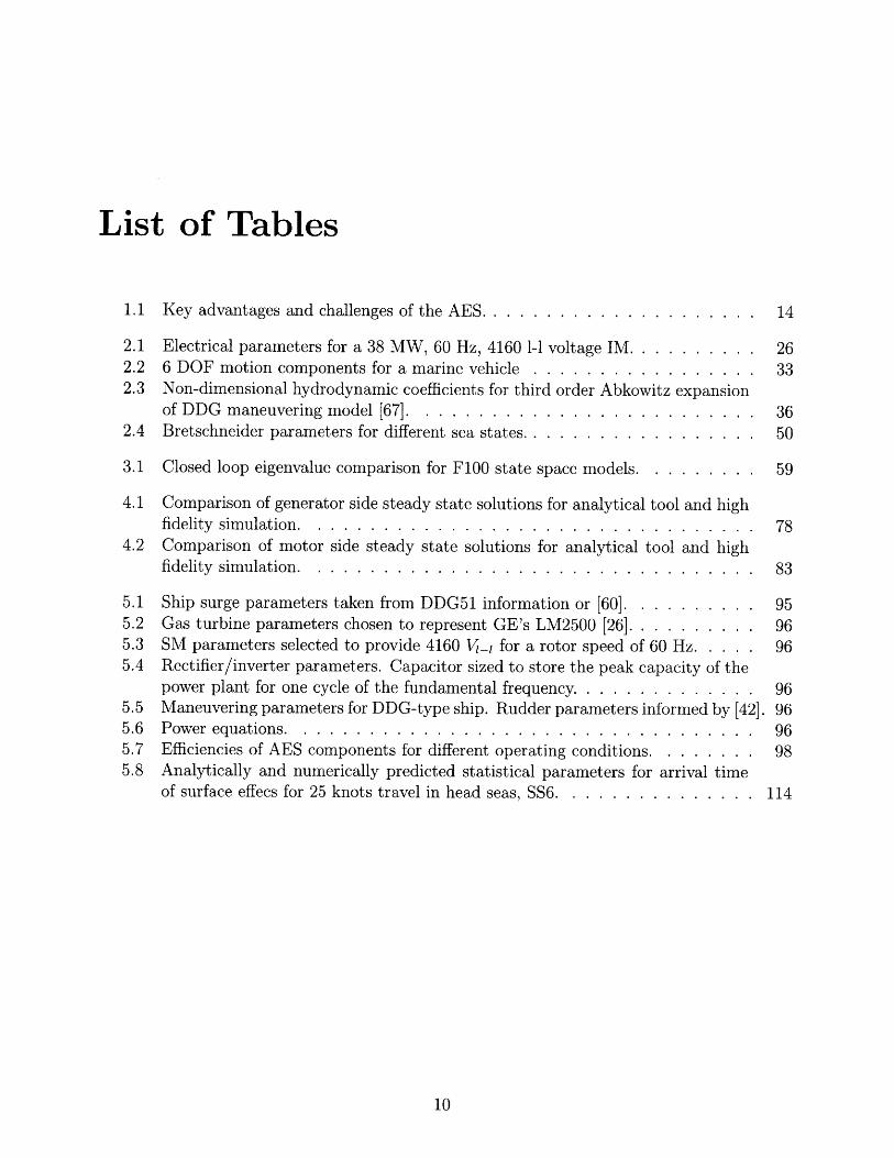
1.1 Key advantages and challenges of the AES. . . . . . . . . . . . . . . . . . . . . 14

2.1 Electrical parameters for a 38 MW, 60 Hz, 4160 1-1 voltage IM. . . . . . . . . . 262.2 6 DOF motion components for a marine vehicle . . . . . . . . . . . . . . . . . 332.3 Non-dimensional hydrodynamic coefficients for third order Abkowitz expansion

of DDG maneuvering model [67]. . . . . . . . . . . . . . . . . . . . . . . . . . 362.4 Bretschneider parameters for different sea states . . . . . . . . . . . . . . . . . 50

3.1 Closed loop eigenvalue comparison for FlO state space models. . . . . . . . . 59

4.1 Comparison of generator side steady state solutions for analytical tool and highfidelity sim ulation. . . . . . . . . . . . . . . . . . . . . . . . . . . . . . . . . . 78

4.2 Comparison of motor side steady state solutions for analytical tool and highfidelity sim ulation. . . . . . . . . . . . . . . . . . . . . . . . . . . . . . . . . . 83

5.1 Ship surge parameters taken from DDG51 information or [60]. . . . . . . . . . 955.2 Gas turbine parameters chosen to represent GE's LM2500 [26]. . . . . . . . . . 965.3 SM parameters selected to provide 4160 V1_1 for a rotor speed of 60 Hz. . . . . 965.4 Rectifier/inverter parameters. Capacitor sized to store the peak capacity of the

power plant for one cycle of the fundamental frequency. . . . . . . . . . . . . . 965.5 Maneuvering parameters for DDG-type ship. Rudder parameters informed by [42]. 965.6 Power equations. . . . . . . . . . . . . . . . . . . . . . . . . . . . . . . . . . . 965.7 Efficiencies of AES components for different operating conditions. . . . . . . . 985.8 Analytically and numerically predicted statistical parameters for arrival time

of surface effecs for 25 knots travel in head seas, SS6. . . . . . . . . . . . . . . 114

Chapter 1

Introduction

All the research presented in this Master's thesis is in support of the effort to bring an all

electric naval fleet from conception to reality. This work focuses on computational approaches

to early design that run in parallel with physical testing of scale models being conducted by

collaborators nationwide.

The All Electric Ship (AES) typifies the chief aim for this research. It is characterized

by an electrically driven propulsion element that is coupled to the onboard support systems

and weaponry, together called the Integrated Power System (IPS). The main components

of the general IPS are electric generators, power electronics, transmission lines, storage and

filter elements, weaponry and radar, and drive elements, i.e. advanced induction motors or

permanent magnetic motors [41].

Indeed, this paradigm of power system architecture has been actualized on ships of lesser

magnitude for decades, but the AES that is referred to herein is one conceived and designed

for implementation on cruisers and destroyers of the utmost level of scale, maneuverability,

defense, and weapons technology, for example, in the United States, the CG(X) and the DDG

or DD(X) models.

1.1 An Historical Introduction to the All Electric Ship

The history of the United States destroyer is marked by the tireless pursuit of excellence and

innovation. It is this pursuit that has, in the last century, made the US Navy one of the most

dominant and technologically advanced forces in the world, ensuring the safety of our domestic

borders, bestowing the power to intervene for peace overseas, and allowing for reconnaissance

in nearly every major body of water. Still, as history has shown, the next great advancement

is always right around the corner, and it is our obligation to get there first.

Of course, the United States has not always possessed a superior Navy [25]. The first

great push for better US sea forces was a result of Alfred Mahan's affirmation of proper naval

strategy in The Influence of Sea Power on History. Quickly after 1890, Mahan's ideas were

adopted by the US; the government became engaged and proactive in the area of oceans

science, and we never looked back.

The largest-to-date technological advance to ship propulsion came in 1897, with Parson's

patent of the steam turbine. The rotating turbine mechanism superseded that of the recip-

rocating piston mechanism in terms of thermal efficiency and power-to-weight ratio and was

adopted quickly thereafter. This change in power paradigm was a harbinger for the experi-

mentation and research to be done in this area in the century to follow.

The first US destroyers, the Bainbridge-class, were commissioned in the opening years of

the 20th century. Their displaced tonnage was about 500 tons (1/20 of today's generation)

and onboard power about 6 MW. These earlier generations of destroyer were "conceived as a

specialized and rather fragile auxiliary to the battle line, [but] grew into an invaluable general-

purpose warship, known in both world wars for its combination of compactness, hitting power,

and toughness" [25]. Today, the destroyer is perhaps the most critical element to the US Navy

fleet, requiring an optimization of speed, maneuverability, defense/weaponry, endurance, and

survivability.

The decade before and after World War I saw great advancements in destroyer technology.

Some new ships, including the Paulding class, began burning oil instead of coal to bring down

fuel tonnage onboard. Many designs called for more complicated drive systems, with multiple

prime movers and two propellers, to increase the power capacity of the ship. This led to the

first destroyers over 1,000 tons and the first destroyers with over 20 MW of power onboard, i.e.

the Wickes and Clemson classes. With prime mover and drive system technology progressing,

destroyer classes were reaching power levels of beyond 40 MW by the onset of WWII.

The advances to the

destroyer following the 180E FF 1052 El DD %63

war were mainly related to 1 0 DDG 2/7 E FFG 8140 N CG/CGN N CG 47

anti-submarine and anti- D 963 E DDG 51,, 120M

DX

aircraft, resulting in the C-100

guided missile destroyer tE

(DDG) class. The next z 60

major advancement to propul- 40

sion was the replacement 20

of the steam engines with '90 '92 '94 '96 '98 '00 '02 '04 '06 '08 '10 '12 '14 '16 '18 '20Year

GE LM2500 gas turbines

in the mid-1970s, first

with two turbines on the Figure 1-1: Recent past and near future composition of the

FFG-7 class of frigate and surface combatant force [63].

subsequently 4 turbines on the Spruance class of destroyers. This resulted in approximately

15 % more thermal efficiency from the prime movers. The DDG with gas turbine propulsion

is the current standard for US destroyers, as shown in Figure 1-1, but many other systems are

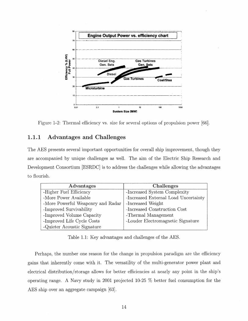
investigated. Hybridization is a popular choice for smaller craft, allowing for high prime mover

efficiencies over the ships entire performance range, see Figure 1-2. Several viable permuta-

tions of steam, gas, diesel, nuclear, and even electric, have been implemented for propulsion

on naval craft, but have yet to be installed on a DDG class warship.

In the last decade, an All Electric Ship has been widely accepted as the next propulsion

paradigm for the US destroyer due to the preponderance of advantages discussed in the sub-

section to follow. Prof. Welsh, Director of the Naval Construction and Engineering program

at MIT, said he does see the AES as the inevitable next step in ship propulsion due to the

improved efficiency and the increased power availability for weapons and radar [73]. "As a

result, the Office of Naval Research established the Electric Ship Research and Development

Consortium in 2002 to stimulate a multidisciplinary approach to the electric naval force system

complexity, and to develop the necessary tools for the complex system design and engineering

to reduce the risk and costs of early decisions" [19].

0Diesel Eng. Gas TurbinesGeni. Sets Gen. Sets0

30- Diesel 00 WOW Gas Turbines CoallStea

Microturbine

to

-0

0.01 0.1 1 10 100 100D

System Size IMWI

Figure 1-2: Thermal efficiency vs. size for several options of propulsion power [66].

1.1.1 Advantages and Challenges

The AES presents several important opportunities for overall ship improvement, though they

are accompanied by unique challenges as well. The aim of the Electric Ship Research and

Development Consortium [ESRDC] is to address the challenges while allowing the advantages

to flourish.

Advantages Challenges-Higher Fuel Efficiency -Increased System Complexity-More Power Available -Increased External Load Uncertainty-More Powerful Weaponry and Radar -Increased Weight-Improved Survivability -Increased Construction Cost-Improved Volume Capacity -Thermal Management-Improved Life Cycle Costs -Louder Electromagnetic Signature-Quieter Acoustic Signature

Table 1.1: Key advantages and challenges of the AES.

Perhaps, the number one reason for the change in propulsion paradigm are the efficiency

gains that inherently come with it. The versatility of the multi-generator power plant and

electrical distribution/storage allows for better efficiencies at nearly any point in the ship's

operating range. A Navy study in 2001 projected 10-25 % better fuel consumption for the

AES ship over an aggregate campaign [63].

The AES also increases the onboard electrical power potential and will allow for large

capacitors able to store unprecedented levels of electrical energy with fast or slow release.

These elements will make next-generation weaponry (like rail guns and high energy lasers)

and next-generation radar (requiring up to 10 times the electrical power necessitated by its

predecessor [73]) a reality. The AES must be realized before these systems can function at

sea.

Other advantages of the AES include increased volume capacity, a new tier of ship surviv-

ability, and improved overhead costs.

The overarching challenge when imagining the AES is the extraordinary system complexity

it will require to accommodate for the scale, the distributed generation and the uncertain

loading [11]. Early AES designs involve a highly intricate and inter-connected IPS, which

will be managing 60-80 MW of power at cruising speeds. At a system level, this effort will

require an optimized distribution and communications topology, a carefully planned grounding

configuration, harmonic mitigation, orchestrated control systems, and redundancies/backup

systems in place in the case of emergency. At the component level, engineers face the hurdle

of designing motors and power electronics robust enough to manage the huge power levels

and transients onboard while incorporating cutting edge technologies like nuclear and fuel cell

power, inventive energy harvesting techniques and new age weaponry and defense systems.

The penultimate challenge arises from the coupling between the propellers and the ship-

board systems. The AES design must take into account the effects of propeller load transients

on the IPS and, likewise, the effects of pulse power loads onboard on the propulsion. Designs

for control and filtering must buffer the propulsion effects from the distribution bus. At its

core, this thesis addresses this challenge.

Other significant challenges include cost, weight, qualification and thermal management.

1.2 Current Focus Areas for AES Research

All ESRDC members meet every May to present work and coordinate efforts for the following

year [21]. The current focus areas presented in Figure 1-3 reflect the latest consortium meeting.

Generally speaking, the largest area of current effort is the conceptualization and selection

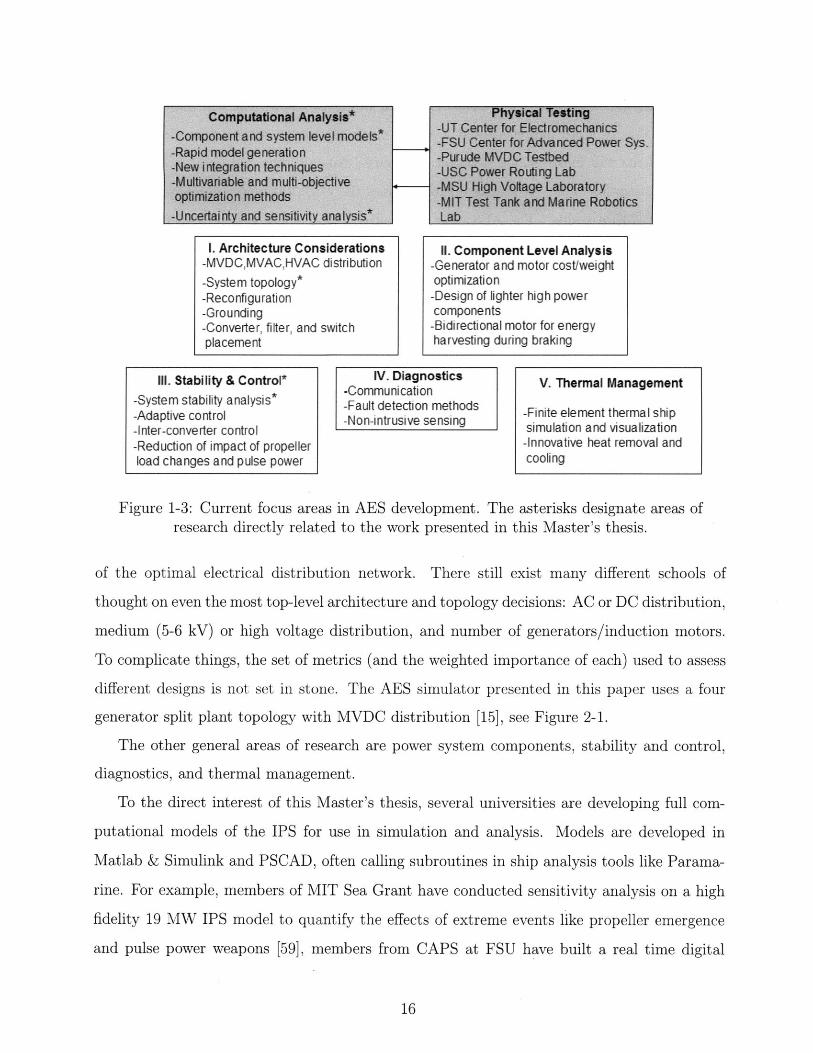
Ill. Stability & Control* IV. Diagnostics V. Thermal Managementanalsis*-Communication-System stability analysis -Famultnetctionmehd-Adaptive control -Fault detection methods -Finite element thermal ship-inter- control -Non-intrusive sensing simulation and visualization-Reduction of impact of propeller -Innovative heat removal andload changes and pulse power cooling

Figure 1-3: Current focus areas in AES development. The asterisks designate areas ofresearch directly related to the work presented in this Master's thesis.

of the optimal electrical distribution network. There still exist many different schools of

thought on even the most top-level architecture and topology decisions: AC or DC distribution,

medium (5-6 kV) or high voltage distribution, and number of generators/induction motors.

To complicate things, the set of metrics (and the weighted importance of each) used to assess

different designs is not set in stone. The AES simulator presented in this paper uses a four

generator split plant topology with MVDC distribution [15], see Figure 2-1.

The other general areas of research are power system components, stability and control,

diagnostics, and thermal management.

To the direct interest of this Master's thesis, several universities are developing full com-

putational models of the IPS for use in simulation and analysis. Models are developed in

Matlab & Simulink and PSCAD, often calling subroutines in ship analysis tools like Parama-

rine. For example, members of MIT Sea Grant have conducted sensitivity analysis on a high

fidelity 19 MW IPS model to quantify the effects of extreme events like propeller emergence

and pulse power weapons [59], members from CAPS at FSU have built a real time digital

I. Architecture Considerations-MVDC,MVAC,HVAC distribution-System topology*-Reconfiguration-Grounding-Converter, filter, and switchplacement

11. Component Level Analysis-Generator and motor cost/weightoptimization-Design of lighter high powercomponents-Bidirectional motor for energyharvesting during braking

simulator (RTDS) electric ship model [3], and members at USC are working on a program for

the rapid evaluation of user-defined IPS topologies [16]. Because of the abundance of electrical

engineers in the ESRDC, these models often fall short on the modeling of the prime mover,

propeller, and ship motion; often, constant assumptions or proxies are used in place of high

fidelity hydrodynamic simulation. A second criticism of IPS models are their long runtimes

due to the level of detail of the electrical component models. These criticisms are attended to

by the work presented in this Masters thesis.

The hydrodynamic simulator presented in this thesis combines nonlinear maneuvering

equations with seakeeping equations, culminating in a 6 degree of freedom (6DOF), time do-

main ship motion simulator. Programs like ASSET [55] and Paramarine are robust analysis

tools for ship design, but cannot to the author's knowledge, conduct event-type time do-

main simulations in 6DOF, in random seaways. LAMP and SWAN are commercial, three

dimensional, time domain ship simulators, but have gained little popularity due to their long

computation times [48]. Perhaps, [22] gives the best presentation of a framework for unified

time domain nonlinear ship simulation in 6DOF; some of its ideas, including the superposition

of low frequency and high frequency motions, are leveraged in this thesis. To the author's

knowledge, however, the program presented in this thesis is the first end-to-end AES simulator

with high fidelity 6DOF hydrodynamic subroutines.

Another direction of research intimately tied to this thesis is the system level stability

analysis of the IPS being approached by several universities. Approaches vary from lineariza-

tion and traditional tools [43], [35], continuation power flow [10], immittance based stability

tests [68] and large-signal stability with Lyapunov theory [45].

1.3 Thesis Deliverables

The statement of deliverables for this thesis is twofold. The first deliverable is a program

for computational AES simulation and analysis. The second deliverable is a program for the

stability analysis of the MVDC IPS.

1.3.1 AES Simulator

The AES simulator is built in MATLAB & Simulink with Fortran subroutines. The model

is conceived with three objectives: true end-to-end functionality, simplification of the IPS

model where plausible, and modularity. The product of this research is a novel, fast AES time

domain simulator capable of predicting, for instance, prime mover fuel consumption for a ship

in a random sea environment, or power bus fluctuation during execution of low radius turn.

The ESRDC has produced dozens of useful IPS models, some of immense detail, for anal-

yses including event simulation, design optimization, and stability analysis. However, because

of the disciplinary make-up of the ESRDC, few of the current models succeed in incorporating

a scheme to access propeller loading in a high fidelity way, as a function of ship motion and

wave elevation. Instead, analyses either use 1) a constant speed assumption for the turbine

and propeller shafts, or 2) first order propeller load proxies (step or hat functions). The

emphasis of the work presented in this thesis is the inclusion of propeller, rudder, and hull hy-

drodynamics in an AES model. At the latest ESRDC meeting, in May 2010, Robert Hebner,

Director of the Center for Electromechanics at The University of Texas at Austin, applauded

these efforts and espoused their growing importance.

IPS models available through the ESRDC exchange tend to offer extremely high fidelity

capabilities, at the expense of runtime and storage proficiency. For example, simulation of

the Purdue Testbed computational model, a scale model of the AES IPS, for 10 seconds in

Simulink rapid accelerator mode, on the author s Dell M1530 laptop, requires about 25 minutes

and a 1.6e6 entry vector for each state (compared to other models, the Purdue Testbed model

is small since it only includes the propulsion subsystem). Runtimes of this magnitude, or

even one order less, are unacceptable for real time simulation and analyses where multiple

simulations are required, namely optimization procedures. For this reason, simplification of

the IPS component models is one of the goals of this work. High order, complex, models have

been replaced with representative, reduced order models. The result is a much more rapid,

less stiff, IPS simulator which still allows for accurate propagation of information across the

system true to second-order effects including power conservation.

The program, in its default state, is composed of low order IPS component models, a

low order propeller model, and high order maneuvering/seakeeping models. The program,

arranged in Simulink with MATLAB and Fortran subroutines, is set up to allow for easy

substitution of higher order models. With this in mind, Chapter 3 suggests higher order models

for the prime mover and the propeller and Chapter 4 presents higher order IPS componentry

models.

1.3.2 Performance and Stability Analysis of the IPS

The analysis tools presented in Chapter 4 of this thesis accompany an effort within the ES-

RDC to assess the stability and performance of the IPS for a wide range of parameters and

operating conditions. Stability is a major concern for the IPS because of the uncertain load-

ing conditions imposed by propellers and the large power transients imposed by high power

weapons. Furthermore, the magnitude of the power system makes the result of instability all

the more catastrophic. The importance of a robust stability tool is due to the relatively large

design space still being considered for AES implementation; the tool should be such that it

can assess a wide range of conditions and identify the degree of stability of each, all in a timely

manner.

The aim of work presented here is an analytical and fairly austere approach to analysis of

an MVDC IPS. The model equations, while nonlinear, are time averaged and simplified where

applicable. Small displacement theory is used to linearize the governing equations and extract

the state space matrices about operating conditions at equilibrium. These matrices become

the engineer's best friend for quick performance and stability analysis.

The IM includes hysteretic elements in its feedback control which complicate the problem.

One method is introduced to assess the performance and stability for systems of this type.

Results are encouraging.

1.4 Outline of Thesis

This thesis is organized into the following chapters:

* Chapter 2 presents the models used in the default program for the gas turbine prime

mover, the IPS including a synchronous machine (SM), power electronics, an induction

motor (IM), and control systems, the propeller, and maneuvering/seakeeping models.

The key contribution of Chapter 2 is a 6DOF time domain ship simulator.

" Chapter 3 presents higher order model alternatives for the prime mover and the propeller.

This chapter is mostly a restatement of others' work, but it is included for the sake of

completeness.

" Chapter 4 attempts performance and stability analyses of the Purude Testbed model,

an example of a MVDC IPS. Small displacement theory is used to conduct the analyses

about equilibrium points. The key contributions of Chapter 4 are validated open loop

state space matrices as well as early closed loop analyses.

* Chapter 5 presents the simulation capabilities of the model presented in Chapter 2

including maneuvering and seakeeping trials in calm and random seaways.

" Chapter 6 summarizes the contributions of this thesis and suggests next steps for the

programs presented.

Chapter 2

An End-to-End Model of the AES

In this chapter, the model components of the AES simulator are described in detail. A

medium voltage, direct current (MVDC) distribution is used; this distribution type is one

favored among ESRDC members [21]. Four LM2500 gas turbines provide approximately 80

MW of power, just as with present day destroyers. The AES model subcomponents are the

prime movers, the IPS, the propeller, maneuvering, and seakeeping, see Figure 2-1. The

two propellers receive power from independent plants; split plant operation [15]. The key

advantage of such an arrangement is the redundancy provided in the event of damage. Each

IPS submodel includes two 22 MW synchronous machine (SM) models, distribution and power

electronic models, and a notional 38 MW IM model. Control systems are described to regulate

turbine speed, bus voltage, IM speed, and ship heading/stability. The maneuvering model is

specific to a hull shape resembling the DDG51. The seakeeping model is for arbitrary hull

shapes.

Some results are shown to verify the models including a demonstration of power conserva-

tion across the IPS, in Chapter 5.

2.1 Gas Turbine Model

Many AES models assume a constant input speed to the electric generator obviating the need

to model the prime mover. One of the incorporations here is simple gas turbine model to drive

the SM. This way, the effects of propeller load changes on the gas turbines can be examined.

lI

Figure 2-1: A schematic of the AES model presented in this thesis.

A first-generation GE LM2500 gas turbine model is used with rated maximum power

output of 21.5 MW, a full-locking torque of approximately 123 kN-m (at full throttle), and

a no-load speed of 6875 rpm (at full throttle) [26]. Torque input of gas turbine is linearly

interpolated with the input shaft speed and fuel flow rate

Ff neQt =Qock Lfa (1 - " )] (2.1)

fmax nt,max

where - is the throttle ratio.

To maintain the turbine speed about n* =60 Hz, a discrete PI feedback control is used to

actuate the throttle, with gains Kp,, and Ki,t. A saturation limit, 0 < L- < 1, is imposedfrax -

to represent machine bounds and a slew rate limiter, _ At, is imposed to prevent engine

surge due to rapid changes in fuel flow rate.

This linear model is sufficient for predicting performance near an operating speed of 60 Hz.

Nonlinear models account for thermodynamic and hydraulic states and can predict machine

limitations, but this is not necessary for the studies conducted in this thesis. In [37], utilities

are provided for the construction of a higher order turbine model. In [36], an experimentally

derived, 23 state, optimally controlled jet turbine model is presented that may be applicable

to shipboard power; this is discussed further in Chapter 3.

2.2 IPS Model

As discussed in Section 1.3.1, efforts were made to reduce the complexity and order of the

IPS, while preserving the average dynamics of the propagation of energy from the propeller

to the prime mover. Time averaged equivalent circuit models for the electric machinery have

been drawn from [46]. The simulation for these equivalent circuits uses a quasi-steady approx-

imation allowing for the use of steady-state sinusoidal analysis with complex impedances. For

a ship system, with high inertia hydrodynamic states, this is well justified by the method of

averaging [29]. Note: the IPS model presented here is accurate only for dynamics with time

constants approximatelyr >> 0.01. Also, all electrical model "states" do not exactly translate

to reality, but are representative of the actual electrical states. Higher fidelity IPS component

models are presented in Chapter 4.

2.2.1 Synchronous Machine

The SM is modeled as an input voltage

source, Ea, a stator resistance, Rg, a

stator winding inductance Lg, and the

separate excitement [46]. The separate

excitement is modeled as a controllable

DC voltage source, Vf, a field resistance,

Rfg, and a field winding inductance, Lfg.

The state equation for the excitement

current is

dif5 1dt I (vf - if Rfg) (2.2)

The rms voltage inputted by a SM

is widely defined as E, = Mgwif/V2, Figure 2-2: Equivalent circuit (SM).

where Mg is the mutual inductance of

the generator windings, w = t is the electrical excitement frequency applied by the turbine,2

and if is the controlled field current. wt is the rotational speed of the turbine shaft, in units

rad/s. The excitement voltage is actuated by a PI controller to maintain a desired bus voltage,

with gains K,,, and Ki,.

The SM produces torque opposing the shaft velocity both from friction and the electromo-

tive force produced by the windings. This model uses a linear friction model, Qfrzc = p1 +pI2Wt.

The electromotive torque created by the generator is formulated to conserve power between

mechanical to electrical domains,

Re{Eai*}Q = 3 , (2.3)

where the numerator represents the real (in-phase) power produced by all three phases of the

SM.

Finally, the state equation for the turbine shaft angular velocity (with shaft inertia It) is

dn~ 60dt - (Qt - (Qfrc + Qg)) (2.4)dt 21t

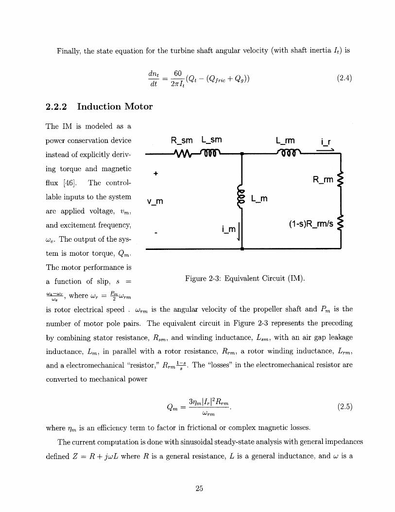
2.2.2 Induction Motor

The IM is modeled as a

power conservation device R-sm L-sm L-rr _r

instead of explicitly deriv-

ing torque and magnetic

flux [46]. The control-

lable inputs to the system

are applied voltage, vm,

and excitement frequency, (1-s)R__n/s

We. The output of the sys-

tem is motor torque, Qm.

The motor performance is

a function of slip, s Figure 2-3: Equivalent Circuit (IM).

WWr where wL s PmLe 2

is rotor electrical speed . Wrm is the angular velocity of the propeller shaft and Pm is the

number of motor pole pairs. The equivalent circuit in Figure 2-3 represents the preceding

by combining stator resistance, Rsm, and winding inductance, Lm, with an air gap leakage

inductance, Lm, in parallel with a rotor resistance, Rpm, a rotor winding inductance, Lrm,

and a electromechanical "resistor," Rrm 1. The "losses" in the electromechanical resistor are

converted to mechanical power

Q 3rmIr|2R". (2.5)Wrm

where r/m is an efficiency term to factor in frictional or complex magnetic losses.

The current computation is done with sinusoidal steady-state analysis with general impedances

defined Z = R + jwL where R is a general resistance, L is a general inductance, and w is a

300 rpm

250 rpm

0 30-30200 rpm

020 - 150 rpm

100 rpm10

50 rpm

0 0.05 0.1 0.15 0.2 0.25 0.3 0.35 0.4Slip

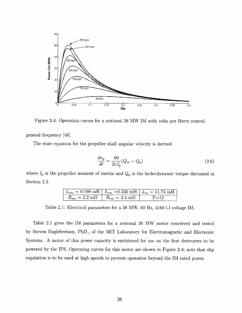
Figure 2-4: Operation curves for a notional 38 MW IM with volts per Hertz control.

general frequency [46].

The state equation for the propeller shaft angular velocity is derived

dnG 60= (0Qm - Q,) (2.6)

dt 27rI,

where Ip is the propeller moment of inertia and Q, is the hydrodynamic torque discussed in

Section 2.3.

L"m = 0.198 mH Lrm =0.330 mH Lm = 11.74 mHRsm = 2.2 mQ Rrm = 3.4 mQ P=12

Table 2.1: Electrical parameters for a 38 MW, 60 Hz, 4160 1-1 voltage IM.

Table 2.1 gives the IM parameters for a notional 38 MW motor conceived and tested

by Steven Englebretson, PhD., of the MIT Laboratory for Electromagnetic and Electronic

Systems. A motor of this power capacity is envisioned for use on the first destroyers to be

powered by the IPS. Operating curves for this motor are shown in Figure 2-4; note that slip

regulation is to be used at high speeds to prevent operation beyond the IM rated power.

2.2.3 Rectification, Transmission, and Inversion Models

DC transmission between the SM and IM in the IPS is favored among ESRDC members

due to its increased power capacity and reduction of transmission losses, among other things.

The pitfall of such an architecture is the inclusion of costly power converters instead of low

cost transformers. While an IPS architecture has not yet been rigidly defined within the

ESRDC, it is the author's experience that the most convincing cases have been made for

MVDC distribution. A MVDC architecture is used in this AES program.

In its simplest form, a MVDC transmission system is composed of a rectifier, inverter,

and power storage element [52]. Additionally, auxiliary loads can be added onto the DC bus

in parallel. Also, filter elements can be included to reduce the transmission of high order

harmonics. The inverter is often composed of controllable switches in order to actuate applied

voltage magnitude and frequency for the purposes of speed or torque control of the motor.

Figure 2-5 shows a general MVDC model equipped with a three phase full-wave rectifier, and

an inverter consisting of ideal switches (approximately attained with IGBTs).

Ea+

Ec

Figure 2-5: Traditional three phase rectifier-inverter [52].

Simulating this model in a high fidelity manner, with true AC states, requires an increase

in computing effort between one and two orders of magnitude. For example, modern power

converters are capable of thousands of ON/OFF cycles per second; modeling these effects

can slow simulation beyond practical use. To maintain the simplicity of the IPS model while

maintaining an acceptable level of fidelity, average models for the power converters, constrained

to uphold power conservation, are used [40]. A schematic of the IPS model for this AES

simulator is shown in Figure 2-6. The average rectifier model consists of diodes. The average

inverter model consists of active IGBTs. A resistance, Rp, is added to the DC bus to add the

effect of losses due to notching. Note: The convention used in the below equations is that Ea

is RMS and line-to-line.

i-gDC LmDC-1 %~

in

Figure 2-6: Schematic of lower order rectifier-inverter model.

The state equation for voltage across the power storage element, ve, is

dve 1(igDC - imDC). (2.7)

If a zero firing angle is assumed, the average DC voltage output of a rectifier can be

approximated as

3 3VDC = V V6Ea - -XCOigDC

7r ?r(2.8)

where Xc, is the commuting reactance of the device [57].

The DC current out of the rectifier, igDC, is found by applying KVL to the loop containing

the rectifier and the capacitor:

.D -VDC - Vc2gDC (2.9)

The inverter DC current, imDC, can be found by asserting power conservation across the

inverter resulting in

imDC 3Re{vmin} (2.10)

where imn is the AC current out of the inverter, to the IM.

Last, power conservation can be added across the rectifier to compute i: Re {3(Ei* - Rpis)} =

VDCigDC-

Note: this model effectively propagates power demands of the motor to the IPS but does not

accurately predict the propagation of IPS loads, like pulse power, to the motor. Essentially,

the motor always gets the power it wants, dictated by the volts per Hertz control. The resulting

required motor power is then propagated back on the IPS by Eq. 2.10. To allow propagation the

other way, a higher order inverter model is necessitated though this is the most computationally

expensive element in all of AES simulation. A clever approximation used here is to add a

dynamic saturation to the motor voltage such that the power drawn cannot exceed the power

available on the right side of the capacitor.

2.2.4 Volts per Hertz IM Control

The actuation of voltage magnitude and frequency by the inverter will likely be achieved with

hysteresis control. It will be assumed that the switching of the controlled inverter is orders

faster than the IM bandwidth. In this case, the average output from the perspective of the

IM can be approximated by a smooth sine wave with a commanded voltage magnitude vm

and command frequency We. The control strategy for selecting vm and We is introduced here.

A volts per Hertz control strategy is used [52]. In this procedure, we is computed using PI

feedback control of the IM rotor speed. vm is then selected to achieve a constant ratio 1.

In greater detail, the command slip speed to the IM, w, is actuated with PI control based

on the rotor velocity error, w* - wr, where w* is the target electrical speed for the rotor. The

excitement frequency delivered to the motor by the rapidly switching inverter is the sum of

the rotor speed and the slip speed command we = Wr + WS.

Dynamic saturation is added to prevent the controlled slip speed, Ws, from becoming greater

than Ws,max, the slip at which the IM torque output peaks. This measure is taken to keep the

control in the monotonically increasing region of the IM torque-slip relationship. An inline

numerical solver is required to solve for ws,max at different rotor speeds. Additional saturation

is added at high speeds to prevent power transmission across the IM greater than its rated 38

MW.

The applied voltage command is related to the excitement frequency linearly, vm = Wt orated

where Wrated and vrated are rated speed and voltage for the motor. This protocol is commonly

employed in IM control and ensures a maximum magnetic flux and results in an identical

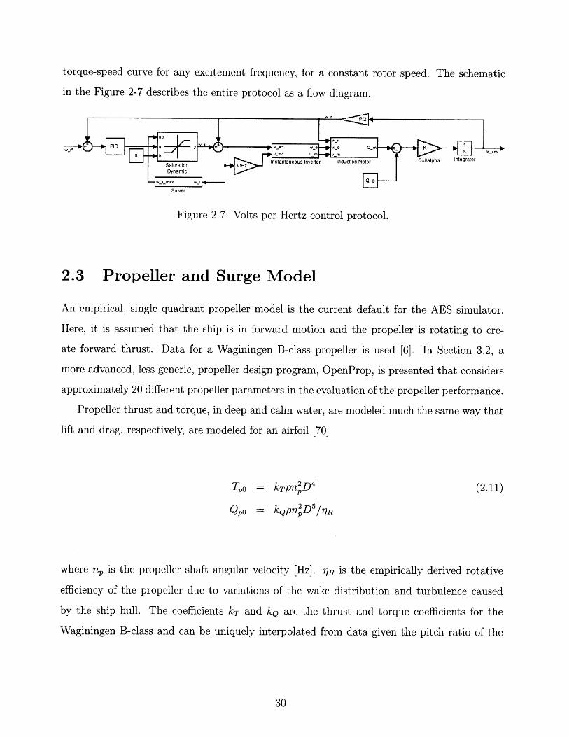
torque-speed curve for any excitement frequency, for a constant rotor speed. The schematic

in the Figure 2-7 describes the entire protocol as a flow diagram.

up

e PID Y we we Qm M -K- 1

Saturation VtHz Instantaneous Inverter Induction Motor Q=I~alpha Integrator

Dynamic

Solver

Figure 2-7: Volts per Hertz control protocol.

2.3 Propeller and Surge Model

An empirical, single quadrant propeller model is the current default for the AES simulator.

Here, it is assumed that the ship is in forward motion and the propeller is rotating to cre-

ate forward thrust. Data for a Waginingen B-class propeller is used [6]. In Section 3.2, a

more advanced, less generic, propeller design program, OpenProp, is presented that considers

approximately 20 different propeller parameters in the evaluation of the propeller performance.

Propeller thrust and torque, in deep and calm water, are modeled much the same way that

lift and drag, respectively, are modeled for an airfoil [70]

TO k pn 2 D 4 (2.11)

Qpo = kQpn 2 D 5 OR

where n is the propeller shaft angular velocity [Hz]. TIR is the empirically derived rotative

efficiency of the propeller due to variations of the wake distribution and turbulence caused

by the ship hull. The coefficients kT and kQ are the thrust and torque coefficients for the

Waginingen B-class and can be uniquely interpolated from data given the pitch ratio of the

propeller and the dimensionless advance coefficient

J U(1 ~ W) (2.12)nD

where u is the ship surge speed and 0 < w < 1 is the experimentally derived wake fraction.

To account for shallow or disturbed water effects, loss coefficients can be introduced to

Eqs. 2.11

T, = 3TkTpn D4 (2.13)

Q, = 3Q kQpn2 D5rR-

In [65] modeling techniques for losses occurring from inflow changes, cavitation, and out-

of-water-effects, are presented. Inflow losses are considered by substituting V, the advance

velocity, for n in Eq. 2.12. Traverse flow effects are not considered in the current version of

the AES simulator.

Out-of-water effects are quantified by

+rcshR 1 (h/R)2"-

TA = Re I - arccos(h/R) h - - (h/R) (2.14)7F iF

where h/R is the ratio of the hub distance to free distance and propeller radius.

Cavitation effects, for high propeller speeds, are hysteretic in nature because there is a

delay in the collapse of ventilation funnel, the vanishing of air cavities on the propeller, and

the build up of blade lift. The Wagner function of lift transience predicts that a foil must travel

20 chord lengths to recover its full lift; for a typical P/D=1 propeller, this is approximately

4 revolutions [56]. A rate limiter is imposed on the recovery of thrust to approximate the

hysteretic behavior. The onset and offset of cavitation effects are taken to be h/R = 1.3 and

h/R = 1.1, respectively. A common total cavitation loss, derived from experiments, is 70

% [65].

The thrust loss coefficient is computed by multiplying the loss effects #T = 3 TA!TV. The

corresponding torque loss coefficient should always be larger than the thrust coefficient so

efficiency is reduced; previous results show the relationship #Q = 3 is sufficient relation for

0 < m < 1 [56]. For an open propeller, m = 0.85 has been applied with success. Figure 2-8

shows the propeller thrust/torque coefficients in a sample wave.

- --h/R

3 - --- p-

2-

Time (s)

Figure 2-8: Demonstration of propeller loss model.

The hull/prop resistance, or fluid drag, has been studied to follow the relationship

1Rs =pCAwu2 /(1 - t) (2.15)

where C, is an empirical parameter of the ship hull which is approximately a constant at the

high value of Reynold's number common to ship travel, A, is the wetted area of the ship, and

t is the experimentally derived thrust deduction. With resistance computed our final state

equation is

dt = (T- R) (2.16)di m + ma,

where m is the ship mass and ma is the mass of the entrained water.

2.4 Nonlinear Maneuvering Model

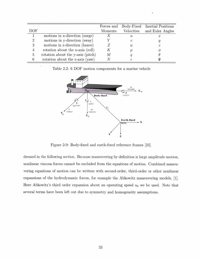
A marine vehicle experiences motions in six degrees of freedom. Employing notation and

graphics from [23], these degrees of freedom are described in Table 2.2 and Figure 2-9.

Maneuvering refers to the study of large amplitude motion of a ship in calm seas. Tra-

ditionally, heave, roll, and pitch are not considered in maneuvering equations due to their

relatively low excitement in calm seas; only planar motions are factored in. Maneuvering

dynamics are distinctly slower than the other variety of ship motions - seakeeping - to be ad-

motions in x-direction (surge)motions in y-direction (sway)motions in z-direction (heave)rotation about the x-axis (roll)

rotation about the y-axis (pitch)rotation about the z-axis (yaw)

Forces and Body-Fixed Inertial PositionsMoments Velocities and Euler Angles

X u xY v yz w zK pM q 9N r T

Table 2.2: 6 DOF motion components for a marine vehicle

& n~0

Body-fixed

P_ U(surge)

(roll)

YS(pitch)

Y (sway) (0

0 Zo

Earth-fixed

Figure 2-9: Body-fixed and earth-fixed reference frames [23].

dressed in the following section. Because maneuvering by definition is large amplitude motion,

nonlinear viscous forces cannot be excluded from the equations of motion. Combined maneu-

vering equations of motion can be written with second-order, third-order or other nonlinear

expansions of the hydrodynamic forces, for example the Abkowitz maneuvering models, [1].

Here Abkowitz's third order expansion about an operating speed uO we be used. Note that

several terms have been left out due to symmetry and homogeneity assumptions.

DOF123456

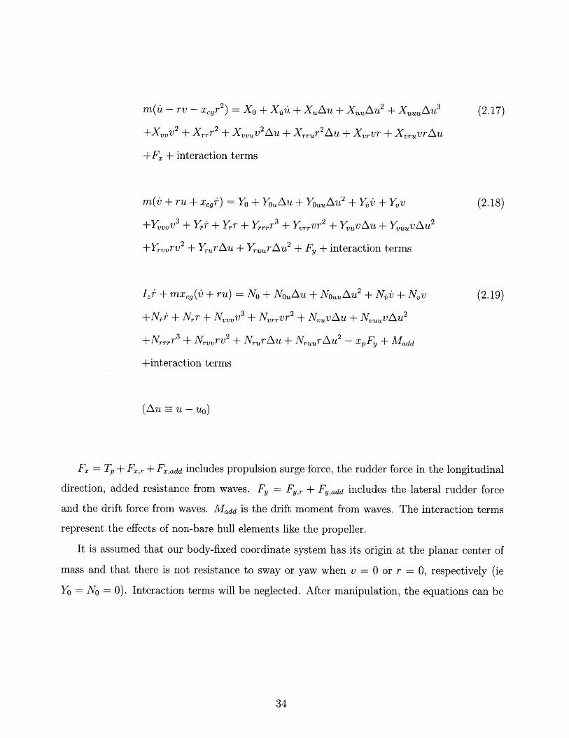
m(i - rv - xcgr 2) = Xo + Xjin + Xu AU + X Au 2 + XUan Au 3 (2.17)

+XvvV 2 + Xr 1,2 + XvvUv 2ZAu + Xrrur 2AU + Xvrvr + Xvruvr u

+Fx + interaction terms

m( + ru + xci) = Y + Yu Au + You0 Au 2 + Y9 + Yvo (2.18)

+YvV3 + Yt + Yr + Y,,r 3 + YvrrVr 2 + Yuv Au + YUUv/ u 2

+Yrvvrv 2 + YrurAu + YruurAu 2 + Fy + interaction terms

IJ ± mx,('b + ru) = No + NouAu + NouuAu 2 + N,'b + Nvv (2.19)

+N i + Nr + Nvvvv 3 + Nvrrvr 2 + NvuvtAu + Nunv Au2

+NrrrT3 + Nrvvrv 2 + Nur u + Nruur Au 2 - xpFy + Madd

+interaction terms

(A~u = - uo)

Fx= T + Fx,r + F,add includes propulsion surge force, the rudder force in the longitudinal

direction, added resistance from waves. Fy = Fy,r + Fy,add includes the lateral rudder force

and the drift force from waves. Madd is the drift moment from waves. The interaction terms

represent the effects of non-bare hull elements like the propeller.

It is assumed that our body-fixed coordinate system has its origin at the planar center of

mass and that there is not resistance to sway or yaw when v = 0 or r = 0, respectively (ie

YO = No = 0). Interaction terms will be neglected. After manipulation, the equations can be

stately as a neat set of ODEs:

M vj=[f2 (2.20)

rf3

where

M - X, 0 0

M m0 M -Y - Y (2.21)

0 -N, IL - Nr

and

f1 = X0 + XUAu + XUUZu 2 + XUUnZ u + XvvV 2 + Xrr 2 (2.22)

+XvvuV 2zAU + Xrrur 2 Au + (m + Xvr)vr + XvruvrZsu + F,

f2 = YouAu + YouuA u 2 + YvV + Yvav3 + (Yr - mu)r + Yrrr 3 (2.23)

+Yvrrvr 2 + YUnvu + YUUvAu 2 + Yrvvrv 2 + YrurLsu + Yruur

Au 2 + Fy

fa= Nou u + Nouusu2 + Nvv + Nr + N ±vvv3 + Nvrvr 2 (2.24)

+NvuvAu + NvuuvAu 2 + Nrrrr ± Nrvv TV 2 + NrurZAu + NruuA sU 2

-- pFy + Mr.

No tractable analytical method exists for the calculation of the hydrodynamic coefficients.

Each new hull shape must be tested experimentally to derive the coefficients. The most

common approach for this purpose is to use a precision measurement machine (PMM). The

coefficients used for this thesis's AES simulator were attained from PMM experimentation of

Surge Value (104) Sway Value (10-') Yaw Value (10--)(Xi - m) -646.9 (Yi, - m) -939.0 N? - I2 -55.08

Xo -65.01 Y 3.216 No -6.813XU -167.3 You 6.836 NoU -17.38XUU -178.1 YUU 3.590 NUU -10.57

Xuuu -80.78 Y -13.17 Nb 16.85(Xvr + m) 93.65 (Yr - mu) -381.6 Nv -308.8

XVV -268.7 Y__ _ -156.8 NvVV -3857

Xrr -101.58 Y -124.6 Nr -219.9X_ -496.4 YVV -39.94 Nrrr -442.0

Xrru -79.74 Yvr -3704 Nvvr -1666

Xvru 117.2 Yvrr -4580 Nvrr -14820

Y _ -2140 Nvu -900.5

YV_ _ -1332 NvUU -671.1

Yru -543.5 Nru -607.0

Yru -111.4 Nruu -561.8

Table 2.3: Non-dimensional hydrodynamic coefficients for third order Abkowitz expansion ofDDG maneuvering model [67].

a 12'2" kayak (the Chesapeake Pro model by Wilderness Systems) by MIT's Jeff Stettler [67].

The coefficients were extracted for trials at nO =2.62 ft/s and uO =5.24 ft/s, or equivalently,

preserving Froude similitude for a DDG51 hull at uo = 11 knots and no =22 knots, respectively.

In ship scale studies like this, Reynolds similitude is not preserved, though operation of the

scale model in the turbulent region is essential; for the 22 knots test, Re = 5.9e6, conditions

are safely in the turbulent region. The results for the 22 knots study will be used and are

presented in Table 2.3.

Figure 2-10 shows a beam comparison of the kayak with the DDG51 model - the similarities

are apparent. Also, the draft for each vessel is near-constant for the majority of the its length.

In [51], this maneuvering model was implemented with coefficients from Stettler and the

computational results were compared with DDG51 sea trials to draw the conclusion of model

accuracy within 10-20 %. Certainly, the transom sterm of the DDG51 will cause conflicts with

the kayak, and refinements could be made with a scale DDG51 model, but this is outside of

the scope of this thesis.

The kinematic transformation to the global reference frame is

Figure 2-10: Beam comparison between DDG51 hull and Chesapeake Pro kayak.

i = ucosV)-vsinO

= usinob+vcoso

The effective inflow velocity and angle are

Va = [U2 + (v + XPr)2]1/2

aa = tan_1 V + xr)u )

(2.25)

(2.26)

(2.27)

where x, is the distance from the body-fixed origin to the stern.

2.4.1 Rudder Model

The rudder is modeled with control surface theory. Notation is given in Figure 2-11. FL is

the lift force and is perpendicular to the inflow. Similarly, FD is the drag force and is parallel

to the inflow. Using a small angle of attack assumption, the lift and drag forces are

FL AVCL where CL a 2.28)2 a@

FD - A, Dwhere CD D (aa -6)2 8

where A is the area of the control surface and 6 is the controlled angle of the control surface.

The lift gradient is approximated using [70]

aCL 1(2.29)

where AR is the aspect ratio of the control surface. For

No.1 rudder shape in [42], the lift gradient is 3.31 and the

drag gradient, tested at a Reynold's number of 1.23e6, is

0.46.

Finally, the lift and drag forces can be converted to the

body-fixed coordinate system

n =sign(aa - 6) (2.30)

F,, = nFL sin a - FDcosa, L

Fy, -nFL cos aa - FD sin a-

D

In marine science, there is a focus on maneuvering con- Figure 2-11: Rudder schematic.trol via rudder or azimuthing propulsor actuation [70], [28].

As a default, this AES simulator will employ saturated PID

control of the rudder angle to meet a heading or to execute

a maneuver. The saturation is added to prevent hydrodynamic stall around 200. A swing rate

limiter A, is added to approximate added mass and damping of the rudder.

2.5 Time Domain Seakeeping Model

Seakeeping refers to the study of wave forces on an arbitrary body at sea and the subsequent

motions of that body. The aim of a seakeeping program like the one developed here is the

prediction of ship motions in regular sinusoidal waves and, using superposition [141, the pre-

diction of responses in irregular waves. The primary attraction of a seakeeping program for

AES analysis is that it allows the relative position of the propeller to be tracked during ma-

neuvers in random seas. Then, employing the propeller loss model discussed in 2.3, the ship

simulation can be coupled to the IPS through propeller loading.

Of course, in ship design, seakeeping performance is one of the most important consider-

ations. In 1970, Salvesen, Tuck, and Faltinsen published a vital paper in the seakeeping field

titled Ship Motions and Sea Loads [62] where they presented a new strip theory for seakeeping

analysis that effectively made the problem analytically tractable and paved the way for the

computational models still used today. Shortly after this paper, MIT combined their strip

theory with conformal mapping techniques for the computation of hydrodynamic sectional co-

efficients, to develop a fully-capable frequency domain seakeeping program called MIT5D [47.

Recently, an MIT graduate student, Ilkay Erselcan, combined their strip theory with Frank's

close-fit method [24] for the computation of hydrodynamic sectional coefficients, to develop

a fully-capable frequency domain seakeeping program [20]. Between, [62], [47], and [20], the

methodology employed in this thesis is covered in detail for first order seakeeping as well as roll

damping. [61] presents a method for the computation of second-order wave effects including

added resistance and drift forces.

Seakeeping is ordinarily presented as Newton's 2nd Law applied in 6DOF with the assump-

tion that the responses are linear and harmonic; the Salvesen, Tuck, and Faltinsen notation will

be used to represent the seakeeping states [ 972 = sway 173 = heave 74 = roll 75 = pitch 76 = yaw

Seakeeping computation in the surge direction is neglected for long slender hull forms because

the hydrodynamic seakeeping forces are much smaller than the viscous friction forces from

maneuvering equations. The general equations of motion are

6

E [( Mk+ Ajk)rik + (Bik + Bjv)rk + Cjk?7k] = Re {Fjeiwt }; j = 2...6 (2.31)k=2

where Myk are components of the generalized mass matrix, Ayk and Bjk are the added mass and

damping (radiation) coefficients, Bj,, are viscous damping coefficients, Ck are the hydrostatic

restoring coefficients, and F are the complex wave excitations. The jk notation indicates

a force in the j direction due to motion or displacement in the k direction. The radiation

coefficients and wave excitations are functions of wave frequency wo, ship speed U, and heading

#. The ship experiences the forces with the encounter frequency

w = WO - kU sin/3 (2.32)

where k is the wave number. For a linear system, the response frequencies should be the same

as the wave encounter frequency.

Now a short description of each relevant force. Added mass accounts for the accelerated

fluid that must be displaced for the body to accelerate; added damping accounts for the

energy loss required to create free surface waves. Froude-Krylov force accounts for the pressure

gradients most substantial in long waves; diffraction accounts for the forces required to disrupt

a wave pattern most substantial in short waves. Viscous wave forces are ignored in ship

seakeeping analysis because of the low relative amplitude of the waves. The restoring forces

are due to buoyancy. All of the above forces are computed with potential theory discussed in

Section 2.5.2. For seakeeping motions, viscous effects have been shown to be significant only

in roll, for instance, friction and separation effects; these will be addressed in Section 2.5.2.

Second-order wave forces for a surface ship are most important in surge, sway, and yaw and

include a constant force as well as oscillatory wave interaction forces; in Section 2.5.4 it will be

seen that these forces are added to the maneuvering equations as opposed to the seakeeping

equations.

The subsections to follow present in some detail the subroutines of this thesis's time do-

main seakeeping program, including 1) the computation of sectional coefficients with MIT5D's

conformal mapping techniques, 2) the use of strip theory to compute response amplitude op-

erators (RAOs) in 5DOF, 3) the calculation of second-order forces, and 4) the generalization

of the frequency domain results to time domain. Results are included in these sections to

show correspondence with their parent papers' results.

2.5.1 Conformal Mapping

MIT5D, a seakeeping program written in the 1970s, is employed to compute the sectional

coefficients using a conformal mapping technique for Lewis and Bulb forms. Though the

section geometry for the conformal mapping technique is not as flexible as Frank's closed

fit method, conformal mapping provides a much faster runtime and does not break down at

critical frequencies. In this section, the key theoretical points will be discussed.

Conformal mapping is the mathematical transformation of one complex function to another

while preserving all infinitesimal angles. In hydrodynamics, a conformal map can be used to

map between a potential flow problem about a convenient geometry and one without, while

preserving Laplace's equation and boundary conditions. For instance, if one can find a the

proper conformal mapping function f : #cyj -> Ox, it can be used to attain a valid potential

field #x from the classic half-cylinder solution #cy. #cyj is a potential that satisfies the linear

boundary conditions for an oscillating half-cylinder and was originally presented in [341.

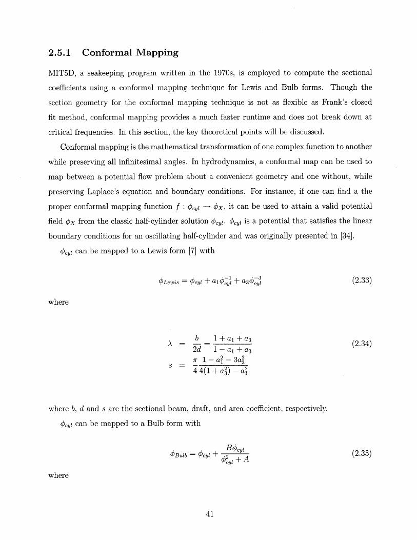
#cyi can be mapped to a Lewis form [7] with

#Lewis = #cyl + a1qy1j + a3 (233)

where

b _1+a 1 +asA = - =3 (2.34)

2d 1-ai+a37r 1 - a2 - 3a2

s=4 4(1 + a3) - al

where b, d and s are the sectional beam, draft, and area coefficient, respectively.

#cy, can be mapped to a Bulb form with

#Bulb = #cyl + 2~c+ (2.35)hcyr + A

where

1--A2 +±AB±BA = -A 2 +AR-B (2.36)

1-- A2+ AB- B

= (1+A1-)4 2A

The pressure per length can be found for each section by substituting the sectional po-

tentials into the unsteady Bernoulli equation and linearizing about the mean hull position.

Sectional coefficients and forces are attained by integrating the sectional pressures on the mean

section boundary assuming that only small displacements of the boundary occur.

In Figures 2-12 and 2-13, MIT5D derived sectional added mass/damping in sway and

heave are shown. These results are nearly identical to those presented in Vugts famous 1968

experiments [711.

2 1

1.5 -- 0.8 - -

0.6 --

0.4

0.50.2 00.5 - -0.2 -

00 0.5 1 5 2 00 0.5 1 15 2

Figure 2-12: Non-dimensional sectional added mass and damping in sway direction for ahalf-cylinder.

2.5.2 Strip Theory

The strip theory equations used in the AES simulator are taken verbatim from the original

strip theory paper by Salvesen, Tuck and Faltinsen. The same right-handed coordinate system

is used, fixed such that the z-axis is vertically upward through the ship center of gravity and

the x-axis runs the ships longitudinal axis, on the undisturbed free surface.

Begin with Eq. 2.31. If the ship has lateral symmetry, the equations of motion reduce to

two coupled sets of ordinary differential equations. The heave-pitch set

2.5 1

2- 0.8-

< 1.5 -£- 0.6-

d 1 - 0.4

0.5 - 0.2-

0 00 0.5 1 1.5 2 0 0.5 1 1.5 2

Figure 2-13: Non-dimensional sectional added mass and damping in heave direction for ahalf-cylinder.

(M + A33 )#j + B33r 3 + C33 73 + As 5#)j + B35r 5 + C3 5 = F3eiwt (2.37)

A53 3 + B53A 3 + C53 I3 + (15 + A55) 5 + BAs5 + C55Q5 = FseiWt (2.38)

and the sway-roll-yaw set

(M + A 22)#j + B 22 )2 + (A 24 - Mze)1 4 + B 24 j4 + A 26 6 + B 26r 6 = F2eiWt (2.39)

(A42 - Mze) #j2 + B42 j2 + (14 + A 44)4 + B44rj 4 (2.40)

+C44 4 ± (A 46 - 146)#6 + B 46 j6 = F4eiwt

A62 #2 + B62r 2 + (A64 - 146)j4 + B64A4 + (A66 + 16)# + B 66 j6 = F6eiWt (2.41)

where z, is the distance from the waterline to the ship's cross-sectional center of gravity.

The basis of modern strip theory is as follows: by making the assumptions that 1) the beam

of the ship varies smoothly and 2) the waves generated by the ship are short in comparison to

its length, one can accurately reduce the three-dimensional problem to an integration of two

dimensional problems, so long as the increment between two-dimensional sections is sufficiently

small (usually accomplished with 20 ship sections). That is, all the aggregate ship coefficients

in the equations of motion above can be computed by integrating the sectional coefficients

and adding speed effects to satisfy the boundary condition of the translating ship. All of the

strip theory coefficient equations are given in Appendix A; for details of their derivation, see

Appendix 1 of [62].

If one assumes that the responses are harmonic with frequency W,

S= Iq I sin(wt + Z), (2.42)

then substitutes, and cancels, the set of second order ODEs reduce to linear equations [69].

Complex response amplitude operators (RAOs) can be computed by solving the resulting sets

of linear equations at any discrete set of w, U and 3:

1

The remaining issue is the nonlinear roll damping introduced as B*4 in Eq. 18 in Ap-

pendix A. The nonlinear damping coefficient contains components from a variety of different

mechanisms including skin friction, eddy making dissipation, and bilge keel separation, [323.

In general, these added damping forces are quadratic in nature

F*= (2.44)

where J is a function of hull geometry and roughness solved for analytically or with look-

up tables. To fit into the linear framework accurately, B*4 is chosen such that the energy

dissipation per cycle is the same as the quadratic case:

I342I 4|dt JB* 4 4 2dt. (2.45)

After assuming a harmonic roll motion, Eq. 2.45 can be satisfied by B*4 = 83(w)| j 4 |. To

solve for B*4, an iterative procedure is used. First, a guess is given for the roll amplitude,

il. Then B* is computed, substituted into Eq. 18 in Appendix A, and a new roll amplitude

|9+1 I is solved for with linear RAOs. B*g+1 is recomputed at the new roll amplitude. This is

continued until convergence is achieved.

In Figures 2-14 and 2-15, normalized RAOs are shown for a half-cylinder, for each of the

5DOF; all RAOs are at a ship speed of 25 knots. These results match well with physical

experiments and other numerical results. Electronic comparison has been conducted success-

fully against results attained from an independent program written by a fellow MIT graduate

student [20].

1.4 1.4

1.2- 1,2 - 0-30

t- - - -1200.8 - 0.8 ~--- 150- - - 180

- 06 0.6-

0.4 It04AV

0.2 -i 0.2 -

0 0.5 1 1.5 0 0.5 1 1.5Wave Frequency (rad/s) Wave Frequency (rad/s)

Figure 2-14: RAOs for half-cylinder in heave and pitch.

Sway, roll, and yaw results are not shown for seas less than 90 degrees because strip

theory appears to break down as encounter frequencies approach zero. As wo -+ kUcos,

the predicted RAOs spike to, in some cases, greater than 10. This is of low concern to this

AES research because it is only heave and pitch dynamics used to assess the propeller loading

changes due to surface effects. In [30], a more accurate procedure for following seas simulation

is given.

Experiments with the DDG51 hull give heave and pitch results that compare well with the

seakeeping programs of others. However, as wo -+ 0 the pitch RAO does not converge properly

(at the same rate at the wave number). This will be acceptable for the time simulator since

there are no wind waves and accordingly only a very small fraction of the wave components

have energy at frequencies below 0.25 rad/s.

2.5.3 Second Order Forces

The seakeeping analysis presented above only accounts for first order wave forces. While

second-order wave forces are in general much smaller in magnitude, they, unlike the first-order

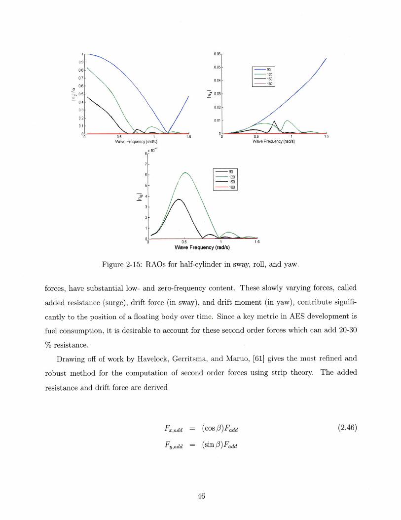
0.0

0.05

0.04

-90-120-150-- 180

0.5- * 003-

0.4 -0.02

0.3-

0.2- 0.01-

0 1- 0

0 0.5 1 1.5 0 0.5 1 1.5Wave Frequency (rad/s) Wave Frequency (rad/s)

x 10'48 -

7 -

-- 906 120

-- -150

4 -

3 -

2 -

1-

00 0.5 1 1.5

Wave Frequency (rad/s)

Figure 2-15: RAOs for half-cylinder in sway, roll, and yaw.

forces, have substantial low- and zero-frequency content. These slowly varying forces, called

added resistance (surge), drift force (in sway), and drift moment (in yaw), contribute signifi-

cantly to the position of a floating body over time. Since a key metric in AES development is

fuel consumption, it is desirable to account for these second order forces which can add 20-30

% resistance.

Drawing off of work by Havelock, Gerritsma, and Maruo, [61] gives the most refined and

robust method for the computation of second order forces using strip theory. The added

resistance and drift force are derived

Fx,add = (cos #)Fadd (2.46)

Fy,add = (sin )Fadd

where

6.

Fa(W, U,3) = k ( ,) (2.47)Fad(,2 ~j(Sj) + FP) + F7.j=2

(Fj)' is the complex conjugate of the Froude-Krylov wave force component. FjP is the

same as the diffraction wave force component, but derived with the complex conjugate of the

wave potential. Then, F7 is

F7 = 2a k I e~ 2kds(b 3 3 sin 2 b22)d<. (2.48)2 w

In Figure 2-16, added resistance and drift force results are compared with [61] to demon-

strate proper implementation.

Added Resistance at Fr.1 92 for Mariner Hul at Different Headings Drift Force at Fr=. 194 of Mariner Hull at Different Headings

S alvesen - 105 - Savesen - 105a / a -120 18 - -120a15 -/150

7 - 180 16 - - - MIT5D - 1050--120

S

a L~14 I -1506 - \ /

/. . 0.a. 1. .4 16 . 2 0 / 6 0 1 1

3 a

2 24

0.0 . 14 1 62 0.4 0.6 068 1.2 1.4lambda/L lambda/L

Figure 2-16: Second order force result comparison with [61].

2.5.4 Time Domain Generalization

In this section, the theoretical groundwork is laid for the generalization of frequency domain

seakeeping equations to time domain equations. Then, the random sea model is described.

Finally, practical simulation issues are addressed.

This simulator applies a quasi-steady approach for time domain simulation. True time

domain solutions to seakeeping have been derived which satisfy boundary conditions for the

instantaneous hull position, allowing for larger amplitude motion fidelity [5]. They are not

applied here due to their complexity and larger computational effort.

Begin with the second-order ODEs for heave-pitch in discrete seas with frequency wo,

amplitude a, and phase 7, and direction p. Assuming the ship is stationary and oriented in

the direction of the global x-axis

(M + A33)#e + B33A 3 + C3373 + A35 5 + B3545 + C35 775 = aF3 eiot+ (2.49)

A53 # + B533 3 + C5393 + (15 + A55)#e + B5545 + C5s7s = aseiwot+ (2.50)

The added mass and damping are functions of the wave frequency, for instance A33 (wo).

The unit wave excitements are functions of both wave frequency and wave direction, for

instance F3 (wo., P). For the remainder of this derivation, a matrix form will be used

d2d[M35 + A35 dt2q35 + C335 = aF5seiot+y. (2.51)

If the ship is not stationary, for instance with speed U and heading T, the equation becomes

2d[M35 + A 35] d-35 + B 3 5 -73 5 + C 357'5 = aF 3setk(xcosI+ysinII)+7 (2.52)

dt2 dt

where the encounter frequency w = Iwo - kU cos 131 and 13 = ' - p. x and y are the global

coordinates of the ship as determined by the maneuvering equations. Now the added mass and

damping matrices are functions of encounter frequency and speed, for instance A3 5 (w, U), and

the unit wave excitement is a function of encounter frequency, speed, and heading, F3 5 (w, U, 13).

A solution for this equation, assuming a steady speed and heading, can be attained by

assuming that the heave and pitch responses are harmonic with frequency w:

q3(t) = a|5 3(w, U,)|cos(wt - k(xcosp + ysin p) + y + ZH3(w, U, 3)) (2.53)

75 (t) = as(w, U, #)| cos(wt - k(x cos p + y sin p) + 7 + ZIs(w, U,#))

where |H3 | is the unit response magnitude and ZHj is the response phase delay for state j.

After substitution, rearrangement, and cancelling, an expression is attained for the complex

response amplitude operator of both heave and pitch

H3(w, U, 2) F35(w, U, 3) (2.54)H(w, U, W) ~-2 [M35 + A35 (w, U)] + iwB35(w, U) + C35

When coupled with the maneuvering model, the speed and heading of the ship become

time variant. A quasi-steady approach for the seakeeping simulation in the time domain is

used

rq3 (t) =fH 3 (w, U(t), /3(t))| cos(wt - k(x cos y + y sin p) + -y + Z# 3 (w, U(t), /3(t)) (2.55)

r5 (t) = ajH(w, U(t), 3(t))| cos(wt - k(x cos y + y sin p) + 7 + L 5(w, U(t), 0(t)).

The wave surface elevation at the stern, by the propeller, is

m,(t) = a(wt - k[(x - x, cos(T)) cos y + (y - x, sin(T)) sin/p] + 7). (2.56)

Finally, the distance from the propeller hub to the free surface is

'Iprop(t) = ho + '7s(t) - r 3 (t) + xrs(t) (2.57)

where ho is the calm water distance.

This quasi-steady approach is acceptable for large ships because of the vastly different time

constants between the maneuvering and seakeeping states. The changes in speed and heading

occur very slowly so the seakeeping dynamics due to these changes are negligible.

The Bretschneider spectrum is used for random wave generation

S(wo) = 5w 1 H (2.58)16 w0

SeaState w, (rad/s) H1/ 3 (ft)2 0.997 0.9843 0.838 2.9524 0.714 6.2325 0.648 10.8246 0.507 16.400

Table 2.4: Bretschneider parameters for different sea states.

where w, is the peak frequency and H1/ 3 is the significant wave height.

Bretscneider parameters for a variety of sea states [31]. Figure 2-17 shows

different sea states.

CN

C,,

0.2 0.4 0.6 0.6 1 1.2

Wave Frequency (rad/s)

Table 2.4 shows

the spectrums for

1.4 1.6 1.8

Figure 2-17: Bretschneider spectrums for different sea states.

Wave frequencies and amplitudes are conventionally sampled from a spectrum using the

following procedure. First, the number of components N, is selected; for seakeeping programs,

100 < N, < 500. Next, spectrum bounds are selected, Wmin and wmax. The spectrum is

than uniformly stratified with increment 6 w = (Wmax - Wmin)/N,. Each of the strata are

sampled randomly to get the wave frequencies wo = [Woi, w02, ... , WoN,]. The paired amplitudes

are selected so that the sampled wave has the same energy content as the spectrum, ci =

0/2S(woi)6w.

A cosh(Ap) spreading function is added to the discrete user-inputted wave direction y to

add more fidelity to the random sea model. h is a parameter that defines the bandwidth of

the spreading function. Values of Ap are sampled with a rejection sampling method. The set

of N, wave directions are computed pi = y- + Api.

N, wave phases are selected randomly from a uniform distribution.

For each wave component zi(x, y, t) = a cos(woit- k(x cos pi+y sin pti) +yi), the seakeeping

analysis is computed and the motions are superimposed.

N 8

rt = a~i|| cos (wit - ki(x cos pi + y sin pi) + z At + (2.59)

where wi = woi - kiU cos 4i with 13i = T - pi and ki = w2/g.

The time domain second order forces are modeled using Newman's first approximation to

slowly varying second order forces [541:

N.

W(t, , U, 13) = a Fadd(wi, U, 3) (2.60)i=1

N, M.<Ns

+ 2Z a i j Fadd 2, U, # cos(( - wj)t + yi + yj + Ai - Aj)i=1 j=1

where Ai represents the lag or lead of wave component i due to the ships global position, not

shown for the sake of space.

The seakeeping analysis is not done serially with the time integration of the seakeeping-

maneuvering model for practical reasons; this simulation framework would require hours, if not

days, to carry out simulations over only a few wave periods. Instead, all seakeeping analysis is

carried out pre-simulation. Added mass and damping coefficients are stored in 2-dimensional

matrices indexed by encounter frequency and ship speed. First and second order wave forces

and RAOs are stored in 3-dimensional matrices indexed by wave frequency, ship speed, and

ship heading. For each time step, the RAO matrix is interpolated for each wave component,

superimposing each motion component to attain instantaneous motions. For each time step,

Newman's approximation is used to attain the instantaneous second-order forces.

Results are given in Chapter 5 for the results of the seakeeping-maneuvering model coupled

with the IPS.

Chapter 3

High Fidelity Component Model

Alternatives

In Chapter 2, descriptions were given for submodels of the default end-to-end AES simulator.

While the AES simulator boasts high order maneuvering and seakeeping submodels, the prime

mover, IPS, and propeller submodels are relatively low order.

The choice of low order modeling leads to extremely fast runtimes allowing for iterative

simulation analysis like optimization or statistical analysis by way of Monte Carlo simulation.

Of course, there is no free lunch. Lower order models try to capture the fundamental input-

output dynamics of a model by reducing, combining, and averaging the internal states, but

often, on top of losing explicit internal state information, model fidelity is compromised. For

the sake of completeness, the next subsections will present higher order models for the prime

mover and the propeller. Higher order models for IPS componentry are discussed in Chapter

4.

* The low order gas turbine model employed by the AES simulator uses the quasi-steady

application of a speed-torque-throttle curve, a dynamic turbine shaft, and PI speed

control. This model provides a good fidelity representation of the key prime mover

dynamics and a working feedback control system. However, the higher order model

presented here 1) functions with optimal control and 2) includes thermodynamic and

hydraulic states allowing for the prediction of machine limitations, engine surge, and

failures.

" The low order IPS submodel employed by the AES simulator is a time-averaged, com-

bined phase representation of the true IPS. It is accurate to second-order effects across

the IPS, like the conservation of power, but its internal states are not explicitly rep-

resentative of physical states. The higher order model presented in Chapter 4 includes

the true AC dynamics, three-phase electric machinery, true inverter switching dynamics,

and current hysteresis control of the induction motor. This model predicts 1) physically

representative internal state information and 2) higher order harmonic effects, both at

the expense of runtime.

" The low order propeller submodel employed by the AES simulator uses the quasi-steady

application of kq-kt curves for a generic Waginingen B-class propeller in open sea. Cav-

itation effects are estimated with a first-order approximation. Traverse flow effects are

not captured. The higher order modeling techniques discussed here provide 1) more

degrees of freedom for the propeller model and 2) propeller flow dynamics.

3.1 A LQG-LTR Controlled Jet Turbine Model

In Kappos 1983 thesis [36], a linearized 23 state, 4 input, 4 output, F-100 jet turbine model is

presented. The paper goes on to do modal decomposition on the full order model, eliminating

the modes with low magnitude and the modes significantly faster than the target control

bandwidth. This process as a whole is called model reduction. The result is a 17 state

system to be used for controller design. The control is a multi-input multi-output (MIMO)

linear-quadratic Gaussian - loop transfer recovery (LQG-LTR) controller. Loop shaping of

the singular value curves is used to deduce the Kalman filter gain matrix and loop transfer

recovery is used to recover the open loop Kalman filter model singular value curves when

linear quadratic regression (LQR) feedback control is added.

In its Appendix, Kappos gives the closed loop state space matrices. When implemented,

these matrices do not elicit the results given in the body of the paper; in fact, the result

turns out to be instable. Efforts were made in this Master's thesis to repeat the mathematical

procedures for LQG derivation, detailed in [36], in order to attain a working closed loop

system.

3.1.1 Development of LQG-LTR Controller

Figure 3-1 shows the closed loop framework for the control of the jet turbine as designed by

Kappos.

X X+ i K )Gs

Kalrnan Filter on Reduced Integrator Full O0rder Model

Order Model

Figure 3-1: Closed loop schematic for LQG-LTR controlled F-100.

The plant model G(s) = Cg(sI - Ag)- 1Bg is a linearized 23 state model of the jet turbine

about an operating point (0.92 throttle). G(s) has four inputs (throttle, stator vane angle,

fan vane angle and nozzle exit radius) and four measureable outputs (compressor speed, fan

speed, compressor discharge pressure, and fan inlet pressure). The measureable outputs are

controlled by a LQG-LTR controller which uses a reduced order model of the jet turbine for

the Kalman filter design; the reduced order model is achieved with model reduction of the full

order system. For notation's sake, the state space representation for the reduced order model

is given:

-(t) = Fgz(t) + Ggu(t) (3.1)

y(t) = Hgz(t) + Dgu(t).

Traditionally, for LQG controlled systems, the reduced model is integrator augmented.

The controlled state space becomes

0 0 1A , _B= [ C =[D, Hg (3.2)

Kappos gives the open loop full order and reduced order state space matrices Ag, Bg, Cg,

D,, F, Gg and Hg in the Appendix of his paper. These are used for the controller design.

The traditional LQG controller is composed of a linear quadratic regulator for optimal

control and a Kalman filter for noise reduction [2]. The state space equations for the model

are

±(s) = Agx(s) + Bgu(s) (3.3)

y(s) = Cx(s)

f (s) = A. (s) + Bu(s) + Kf (y(s) - y(s)) + Kfr(s)

y = Csi(s)

u(s) (s)

where x(s) and y(s) are the physical states and ouptuts and i(s) and y(s) are the estimated

states and outputs, for an input u(s). r(s) is the reference input.

The objective of loop shaping, as specified in [36], is to select Kf such that the singular

values of Gf(s) = C(sI - A)- 1 Kf have bandwidths between 2 rad/s and 12 rad/s, meeting

the demands of a fast controller while filtering the estimated noise.

The Kalman filter gain matrix is computed Kf = ECTN-1 where N is a tuning parameter

and E is the solution to the algebraic matrix Ricatti equation

AE + EAT + FFT - ECT N-1CET = 0 (3.4)

where F is a second tuning parameter. In the absence of noise data, N and F are free to vary

as tuning parameters. Let N = pI. This way, different values of t shift the singular values

G(w) -1of Gf(s) to different band widths. Furthermore, let F = . This will pinch the

0

singular values of Gf (s) around w,. Trial and error led to y = 5e - 3 and w = 3 rad/s. Figure

3-2 shows the resulting singular value plot of Gf(s). The bandwidth of the singular values are

between 3.5 and 8.4 rad/s.

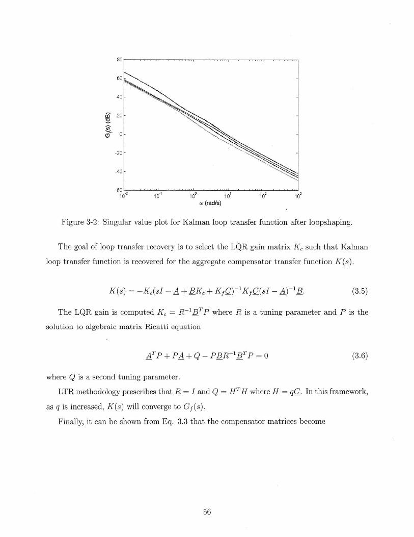
60

40-

20-

0-

-20-

-40-

-60 -

10-2 10~1 100 101 102w (rad/s)

Figure 3-2: Singular value plot for Kalman loop transfer function after loopshaping.

The goal of loop transfer recovery is to select the LQR gain matrix Kc such that Kalman

loop transfer function is recovered for the aggregate compensator transfer function K(s).

K(s) = -Ke(sI - A + BKc + KfC)- 1 Kf C(sI - A)- 1 B. (3.5)

The LQR gain is computed Kc = R-1BTP where R is a tuning parameter and P is the

solution to algebraic matrix Ricatti equation

ATP + PA + Q - PBR-BT P= 0 (3.6)

where Q is a second tuning parameter.

LTR methodology prescribes that R = I and Q = HT H where H = qC. In this framework,

as q is increased, K(s) will converge to Gf(s).

Finally, it can be shown from Eq. 3.3 that the compensator matrices become

Ak = A-BK -KfC (3.7)

Bk = Kf

Ck = Ke

3.1.2 Numerical Results Comparison

With the controller designed, one can look at the open loop singular value plot

(s) G(s) K(s) and the closed loop command-following singular value plot ()= [I +

G(s)!K(s)]-G(s)LK(s). Figure 3-3 shows the results presented in the Kappos thesis. Figure

3-4 shows the results of this thesis.

dB100 0-

0-

-Le

-ISO

100--

20 103 to i e

Figure 3-3: Singular values for Kappos' open and closed loop transfer functions.

To derive the closed loop state space model, start by defining the state vector X -

[Xpiant Xcom Xint]', where Xplant is a vector of the 23 engine model states, Xcom is a vec-

tor of the 17 compensator states, and Xit is a vector of the integrals of the four compensator

outputs. By this convention the linear equations are written

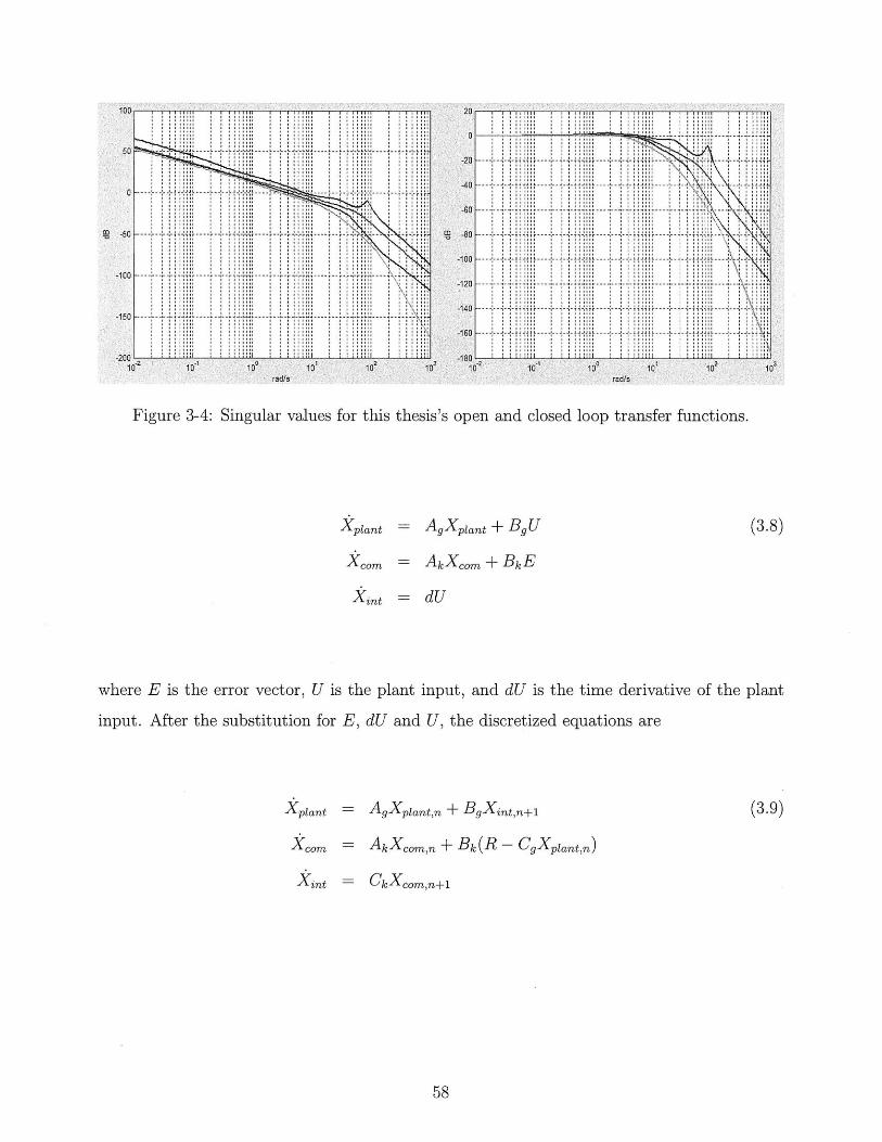
100

5 0

0

o -50

-100

-150

10 10 10 10 102 10

I i i1 I i I 5 i i r r r

T iT I T 7 7 7 T n. 1, - - - - 1 1 1 :T r r 1 1Ii , 1 1 1 1 T

i i i 1 I i i i i I l E I I il I I I I II I E T i I 1

-2

-2

-6-

-12

-14

-10

-18101 10 10 10 10

Figure 3-4: Singular values for this thesis's open and closed loop transfer functions.

(3.8)Xpiant AgXpiant + BgU

Xcom= AkXcom + BkE

Xmt- dU

where E is the error vector, U is the plant input, and dU is the time derivative of the plant

input. After the substitution for E, dU and U, the discretized equations are

X plant

kcom

X int

(3.9)AgXplant,n ± B9X2nt,n+1

SAkXcom,n± Bk(R - CgXplant,n)

- CkXcom,n+1

0-ii r - - - -- - , 11 Tr -- 1 ' T r - - -1 - I I' I l T - ----

4- 4- 1 1 | I'l T r - - - i -- - i-- T - - - il -- - 1- r - - l- -

I i i l i i i i i i i l l { [ | [ i i l i i i 1 [ I E i i | |

- 1 1 T T - -1 - n- n' T 4 44 T r - -n n- aIII f I

| |, , I j j I L - - - - J , I , I 'L - - - - J J I I' j I' I ' ----J, -j, I j L

0 - i 1 t i I i I Egi i i I i l -E I I I i i i I I ti0 - i J $ i i ii1 I a i i i I l i I i I I IIl

0 - i e i i | l l | | | |2 I l I i i 1 i I l i0 - " 1 1 7 " "- r" 3 3 T "1 E """"i""a" "T 3 I l"" - ""T "" "'""""h T 3 T

0 - i l i I i iiri l i a e iI 1 1 f 1 ,0 - riii i e i iiitii i

0-

Kappos Appendix-0.473-0.548-0.649-0.926-2.128

-2.25 ± j1.03-2.38 ± j15.90-4.01 ± j12.27

4.605-5.19 ± j3.83

-5.50 t j87.37-11.59 i j22.67-11.82 ± j3.93

-13.73-16.41

-16.82 ± j3.13-19.74 i jO.86

-20.42-20.87-21.34

-21.60 i j38.03-29.26 + j5.52

-42.44-50.00

-50.44 i j29.30-94.33

-177.22-577.02-764.26-7773.7-77101

-2.507e5

Kappos Body-0.475 t jl.83E -

-0.649 ± j6E - 4-1.482 ± jl.40

-2.122-2.127

-4.37 i j4.08-5.34 t j87.60-5.72 i j7.71

-8.31 i j25.85-8.58 ± j7.09

-11.77 j1.94-13.57-16.44

-17.92 ± j4.82-18.08 ± j6.28

-19.85-21.38 i j0.842-21.95 ± j0.560-24.56 ± j35.05

-41.62-50.00

-50.21 ± j28.25-93.83-177.24-577.02-764.24-777.35-7710.2-25075

Schmitt-0.474 ± j2.5E - 3

-0.649 i j6E - 4-1.755 ± jl.62

-2.122-2.127

-3.56 ± j2.98-5.14 ± j5.80

-6.29 ± j87.96-7.35 ± j4.41

-9.43 tj23.67-11.78 i jl.20

-12.71-17.02

-17.83 ± j4.79-18.73 + j6.42

-19.82-21.36 i jO.757-22.17 ± jO.208-22.85 ± j34.34

-41.41-49.98

-50.02 ± j27.30-85.35

-177.73-577.02-763.28-7774.9-77104

-250750

Table 3.1: Closed loop eigenvalue comparison for FlO state space models.

Using a first order finite difference approximation for the n + 1 terms, with step size h, the

matrix form is attained

I 0

0 k

0 -hCk

-hB [ Xpiant A 0 B1 Xpiant 0

0 Xcor = -BkCg Ak 0 X O + B R (3.10)

I Xint 0 Ck 0 Xin 0

XpiantwithY=[O Cg 0] XO .

XintBy setting h to zero one attains the closed loop continuous state space model. In Table

3.1, ordered eigenvalues are given for three closed loop A matrices: 1) the A matrix formed

from the plant and compensator matrices given in Kappos's Appendix, 2) eigenvalue results

presented by Kappos in the body of the paper, and 3) results from this thesis's re-derivation.

Notice that the matrices given in Kappos's Appendix lead to a slightly different eigen-footprint

that includes an instable pole (4.605).

The new closed loop state space matrices for the LQG-LTR compensator are given in

Appendix B. The B matrix is structured to input the four input commands and the C matrix

to return the four outputs.

3.1.3 From Jet Turbine Model to Electrical Generation Model

It would be a shame to let the F100 data go to waste. Here the use of an altered F100 model

for a gas turbine model to be used with the AES simulator is speculated.

First is a comparison of the power output of the F100 model and the LM2500. The dry

thrust of the a F100 engine is 79.1 kN with an exit diameter of approximately 1 m2 [58]. If

it is assumed that the gas turbine captures most of the jet turbine exhaust, one gets a rough

number for the power of the hypothetical converted F100 gas turbine of 18.6 MW. This is

comparable to the LM2500.

Physically speaking, the significant difference between a jet turbine and a gas turbine is

the addition of a third stage of compensators that are designed to turn the thrust energy of

the exhaust into rotational energy. In fact, many jet turbines are modified this way after their

lifetime on a plane expires. The actuated inputs and measured outputs used by the F100

model are realistic for a gas turbine, however turbine shaft speed would invariably be included

in the feedback control [37].

The method suggested in this thesis is to augment the full plant model with a state for

the turbine shaft speed

-Itbt = Qt - Qg (3.11)

where Qt is an algebraic function of the jet turbine states cleverly chosen to be physically

realistic. For instance, if one could gather data for the compressor turbine and nozzle geometry

on the F100, one could approximate the exhaust velocity algebraically from the compressor

speed using classical turbine mechanics [37]. Then, assuming a gas turbine blade geometry,

one could approximate the torque Qt from the exhaust velocity. It could then be selected to

meet an operating speed of 60 Hz. The dynamics that would be lost would be for fluid flow

states likely to be much faster than the dominant mechanical states. Then, instead of using

compressor speed feedback, one would could turbine speed feedback.

With this new augmented model, all the steps of Kappos's thesis would need to be repeated

including model reduction, Kalman filter loopshaping, and LTR.

3.2 Advanced Propeller Modeling Techniques

Candidly, the propeller model is the weak point of the model discussed in Chapter 2. Its

generality and lack of dynamics compromise the usefulness of the program. An obvious next

step in the development of the AES simulator is augmentation of the propeller model. For

completeness, here is a discussion of some key additions that could be made.

3.2.1 Vortex Lattice Line Method

OpenPropV2.3 is the latest version of a state of the art propeller design and analysis tool

developed at MIT [18]. The numerical model is based on the vortex lattice lifting line methods

[38]. The design optimization method accepts a propeller geometry and inflow properties,

partitions the propeller into blade elements, and solves for circulation and induced velocities

of each element such that the torque is minimized for a specific thrust. Details are outside of

the scope of this thesis but can be garnered in the references above.

The impressive potential of the program is its large design space including propeller geom-

etry and inflow parameters. Figure 3-5 shows the user interface for the single propeller design

feature of the program.

Number of BladesPropeller Speed (RPM)Propeller Diameter (m)

Required Thrust (N)Ship Velocity (m/s)Hub Diameter (m)Number of Vortex Panels over the RadiusMax. Iterations in Wake AlignmentHub Vortex Radius/Hub RadiusHub Unloading Factor f-OptimumTip Unloading Factotr: 1-Reduced LoadingSwirl Cancellation Factor 1-No CancellationWater Density (kg/m^3)

Shaft Centerline Depth (m)Inflow Variation (m/a)Ideal Angle of Attack (degrees)Number of Points over the Chord

2) Hub Image Flag (Check for YES)I Ducted propeller (Check for YES)

Meanline Type:MACA a=0.8

r/R c/D Cd0.2 0.16 0.0080.3 0.1818 0.0080.4 0.2024 0.0080.5 0.2196 0.0080.6 0.2305 0.0080.7 0.2311 0.0080.8 0.2173 0.0080.9 0.1806 0.0080.95 0.1387 0.008

1 0.001 0.008

Filename PrefixOpenProp

Run OpenProp

1 Thrust Ratio1 Dut Diameter/Prop Diameter

0.008 Duct Section Draq Coefficient

Thickness Form:NACA 6SA010

VaNs VtNs fic tO/c Skew1 0 0.0174 0.2056 01 0 0.0195 0.1551 01 0 0.0192 0.1181 01 0 0.0175 0.0902 01 0 0.0158 0.0694 01 0 0.0143 0.0541 01 0 0.0133 0.0419 01 0 0.0125 0.0332 01 0 0.0115 0.0324 01 0 0 0 0

Figure 3-5: Input screen for OpenProp2.2.

There are base level geometry parameters like diameter and blade number, but also specific

considerations like the thickness, camber, and chord as a function of blade radius, for example.

Furthermore, the program allows for the specification of axial and traverse flow into the

propeller which as discussed previously can be responsible for performance losses.

OpenProp v2.3 does not have a feature to derive kr and kQ curves from geometry alone.

As of the date of this thesis publication, that feature has been developed, and it is planned to

be released in future versions of the code. As soon as this faculty is added, it is recommended

that OpenProp is used as a subroutine of the AES simulator to allow from a rich propeller

design space.

3.2.2 Modern Cavitation Methods

Another area where the propeller model could improve is cavitation prediction accuracy. Cav-

itation is a modeling nightmare due to its viscous two-phase nature, its unpredictable stability,

and its multiple formation mechanisms and manifestations.

As discussed in Chapter 2, the AES simulator uses first order approximation for cavitation

losses. This three parameter model is demonstrated in [65] to be viable against physical

results. The three key parameters are the h/R ratio where cavitation losses begin, the h/R

62002

400005

0.420100001

1025

30.3

1.5420

ratio where cavitation losses reach their maximum, and the maximum cavitation loss factor.

Ideally, these three parameters could be estimated for any propeller shape and speed, though

right now we settle for generic values.

An analytical approximation for cavitation prediction can be achieved after solving the

vortex lattice lifting line equations. By comparing the minimum pressure coefficient on the

propeller surface to the cavitation index, one can predict the onset of cavitation on propeller

blades [38]. It should be noted that these predictions are far from perfect, but would allow

less general parameter selection for the three parameter cavitation model discussed above.

Some attempts to numerically study cavitation ambitiously employ finite element methods

including a propeller surface mesh, a fluid mesh, and a free surface mesh. Some studies with

CFD program Fluent have shown correspondence for surface piercing propellers, but cavitation

prediction for fully submerged propellers has proven unsuccessful so far [8].

Chapter 4

Stability Analysis of the MVDC

Integrated Power System

This chapter presents a multi-purpose computational tool for performance and stability anal-

ysis of a MVDC IPS; in this study the MVDC IPS is modeled after the Purdue MVDC

Testbed [4]. An austere approach to stability analysis is taken: nonlinear models are defined,

steady state operating points are solved, and small displacement theory is used to linearize

the system about the operating point and assess the performance and stability for open loop

operation. Closed loop analysis is explored but not entirely resolved.

Figure 4-1: A schematic of the Purdue MVDC Testbed [49].

Let's briefly review the Purude MVDC Testbed (featured in Figure 4-1). In this study,

the generator has been augmented with a linear gas turbine model and the motor with a

quadratic propeller model, both presented in Chapter 2. Accordingly, the inputs of system

are target turbine speed, target DC bus voltage, and target torque. The measured states used

in feedback control are DC voltage, DC current, motor torque, and motor current magnitude.

The actuatable states are the synchronous generator field voltage and the inverter switching

pattern. This analysis is made more tractable by splitting the generator side from the induction

motor side, eliminating the coupling between the sides at the inverter. Accordingly, the study

poses the question: "if the generator is running at operation conditions, what is the stability

and performance of the motor side, and visa versa?" For generator side analysis, the motor

side is modeled as a current sink with magnitude I. For the motor side analysis, the generator

side is modeled as a voltage source Vdc. A method for combining the generator and motor

sides is given in [64].

The capabilities of this tool include but are not limited to time-averaged models for gen-

erator and motor sides (Section 4.1), steady-state solvers for system equilibrium points and

linearization about these points with small displacement theory (Section 4.2), stability/per-

formance analysis for the open loop systems (Section 4.3), and in some capacity, the closed

loop systems (Section 4.4). A high fidelity, unaveraged, Purdue MVDC Testbed model, is

incorporated to check results throughout [49].

4.1 Description of IPS Models

"The Purdue [MV]DC Testbed is a voltage and power scaled DC power system with strong

architectural similarities to power systems being investigated for future Navy ships" [4]. It

includes a 59kW wound rotor synchronous machine and a 4-pole, 460 V, 50 Hp, 60Hz induction

motor interfaced through a 3 phase, passive diode rectifier and IGBT inverter. The generator

side is managed by PI droop control of the DC voltage and the motor current supply is

controlled by current hysteresis control.

In this section, descriptions are given for the system components and time-averaged non-

linear equations are presented for the use in stability analysis.

4.1.1 Generator Side Models

A process flow diagram for the generator side is shown in Figure 4.1.1. The main components

are a PI controlled gas turbine, a three phase SM, a passive rectifier, a passive filter, and DC

voltage droop control.

(omega' R 1 L1 R2 L2

- tu rt 0mega

TTurbine Co l mes vde vdc tilde C1 C2 R3

Turnine Rectifier

S Re rus Generator

Field Control

Figure 4-2: Turbine-Generator side process flow diagram.

As will be detailed below, the resulting open loop model involves an eight state set of

differential algebraic equations with five SM current states (ig,qs ig,ds ig,qr ig,dr ifd), electrical

rotor speed w, and distribution voltage and current (vdc idc). The nonlinear constraints are

a product of the time averaged rectifer model, as will be shown. The inputs are the SM

field voltage Vfd and the turbine speed command w* (note, the closed loop turbine control is

included in the open loop model). A third input is the current sink magnitude I reflective of

the operating condition for the induction motor; however, in this analysis, it will be assumed

that I cannot be actuated. I can be approximated to meet some operating condition for the

motor side by applying the power conservation equation across the inverter: vdcI = ormQm.

For the closed loop system, a feedback state is introduced, the time derivative of the droop

control feedback. The input becomes the command DC voltage v*.

Generator Equations

The SM mathematical equations in the rotor DQ reference frame [40] are

PAg,qs Vg,qs + Tg,sig,qs - (4g,.s (1)

pg,ds Vg,ds + r9 ,sig,ds + WAg,qs

PAg,qr Vg,qr - rg,qr'g,qr

PAg,dr Vg,dr - Fg,drIg,dr

PAfd 77fd Tfd? fd

Ag,qs -Lisigqs + Lmq(-ig,qs + ig,qr) (4.2)

Ag,ds -LIsgds + Lmd(- 7 g,ds + ifd + g,dr)

Ag,qr = Lg,qrigqr + Lmq(-ig,qs + ig,qr)

Afd = Lfdifd + Lmd(-ig,ds + t fd + ig,dr)

Ag,dr Lg,drig,dr + Lmd(Zg,ds + ifd + ig,dr)

where A are magnetic fluxes, v are voltages, and i are currents. r and L are resistances and

inductances, respectively. The subscript denotes the d or q reference frame and the stator (s),

rotor (r), mutual (m), or field (fd).

After manipulation, these can be stated as a system of ordinary differential equations with

current states (ig,qs ig,ds ig,qr ig,dr ifd) (these are nonlinear equations due to the freedom of w,

the electrical rotor speed, to vary).

ig,qs Zg,qs 1 0 0

ig,ds ig,ds 0 1 0 Vg,qs

d gk= Mg A ig,qr + Mg-1 0 0 0 Vg,ds (4.3)dIt gq g 1

9 j +Mig,dr ig,dr 0 0 0 [ Vfd j

ifd ifd 0 0 1

(LIs + Lmq)

0

-Lmq

0

-(Li + Lmq)

0

0 Lmd

0 Lfd+ Lmd

Lg,dr + Lmd

Lmd

r8

-w (Lis + Lmq)

0

0

0

w(Lis + Lmd)

r,

0

0

0

0

w Lmq

-rg,qr

0

0

-W Lmd

0

0

-rg,dr

0

-W Lmd

0

0

0

-rfd

(4.5)

Turbine Equations

The equation for the mechanical speed of the rotor shaft stated generally is

dIt -wt = Qt - Qgdt

(4.6)

where the rotor electrical speed is related to the mechanical speed through a pole multiple

Pg

Some control is requred to maintain the shaft speed about an operating point; as in Chapter

2, PI feedback control will be used. Here, torque is actuated instead of throttle but this is

analogous to actuating the throttle in the linear operating region. After substitution of the

PI control and the SM electromagnetic torque equation [40] into 4.6, the equation becomes

where

A -

Lmq

Lg,qr+ Lmq

0

Lmd

0

0

Lmd

0

-Lmd

-Lmd

and

(4.4)

Ag =

dIt We

dtKp,(o* - ot) + Ki,t (Wt - ot)dt (4.7)

3P+ g[(Lm - Lmd)ig,qsig,ds + Lmdig,qstg,dr + Lmdig,qsifd - Lmqig,dsig,qr]

4

Rectifier Equations

The time-averaged equations for the 6-phase rectifier are adapted from [57]. The first equation

quantifies the average output of a 6-phase converter

33v7"c = qs 2 + )2 ds cos a

g7s Td

3- Xeidc (4.8)

where Xc0 represents the commutating reactance of the left side of the rectifier and a is the

firing angle which will be approximated as 0. The value of the parameter Xc0 is not known

apriori and will be estimated from results with the unaveraged rectifier model; this procedure

is discussed in the next section.

Two other equations impose the conservation of real and reactive power.

2og,qszg,qs + o9,dszg,ds = 3 vdciac COS #

2Vg,qsig,ds -- Vy,igqs = -Vdidc sin#3

(4.9)

(4.10)

where # = cos- 1 T - is the power factor of the rectifier.3VV V ,q ds

Filter Equations

The filter model used here is fourth order in voltage and captures the essential frequency

behavior of the actual sixth order filter used in the Purdue MVDC Testbed. R 3 is an auxiliary

load drawing off the bus for experiments with subsystem loads. The equations for the filter,

derived with Kirchoff's laws, are:

4) dtVc + K 3 c + Vd + K 2) (1) d K dc = c - (R1St4VdC VV(I C v dt 2 vv dt2d +V Vd =jd +K 0 V - + R2)(4.11)

K , ic + K (2) c+

K7it + iv dt 2 Vdc + Kz Vdc + K Vdc = v~ac + R21

(4.12)

where

[CiC 2LIL 2]

[C1C2L2R1 + 1C2L1R2 + C1L1L2/R3]

[C1C2R1R 2 + C1L2R1/R3 +C 1L1R2/ 3 + C1L1 +C 2L1 +C2L 2]

[C1 R1 R2/ R3 + R1C1 + R1C2 + L1/R3 + R2 C2 + L2/R3]

[R1/R3+ R2/R3 +1]

K(O

K 2

iv

K(1

K(Oiv

= C2 L 2

C2R2 + L2/R3

R2/ R3 +1.

DC Voltage Droop Control Equations

A robust solution to DC voltage management is PI droop control pictured in Figure 4-3. In

this strategy, some current feedback is added to the voltage feedback to effectively preclude

instability due to the control while accepting a small stationary voltage error. This method

is especially effective with multiple generating units in parallel. The control also includes

anti-windup at saturation.

Ignoring the anti-windup control and the control bias, the equation for the actuation of

K1 d.K " d I*c+

K (2

Figure 4-3: DC bus voltage droop control [49].

the field voltage is

dVfd =Kp, c -Vdc - Kdidc) + K v -Vdc - Kdidc)dt (4.13)

4.1.2 Motor Side Models

A process flow diagram for the system is shown in Figure 4.1.2. The main components are a

three phase IM, IM torque control, an IGBT inverter, and a propeller.

To T PW,7M1 Control Tr

Trim Control 4ATPA Control Propeller Propeller Shaft

T-m )do Reference FrameInduction Motor

Figure 4-4: Motor-Propeller side process flow diagram.

As will be detailed below, the resulting open loop model involves a five state set of ordinary

differential equations including 4 IM current states (im,qs Im,ds t m,qr zm,dr) and the propeller

shaft speed Wrm. The input to the system is the average voltage magnitude seen by the IM

from the rectifier vqs. A second adjustable input is the voltage source Vdc reflective of the

operating condition for the generator side; however, in this analysis, it will be assumed that

vdc cannot be actuated.

For the closed loop system, one state is added, the time derivative of the measured torque.

The input becomes user specified torque command T*.

Motor Equations

The IM mathematical equations in the rotor DQ reference frame [40] are

PAm,qs Vm,qs - rsim,qs - We Amds (4.14)

PAm,ds Vm,ds - rslm,ds + WeAmqs

PAm,qr -rr7m,qr - sAm,dr

pAm,dr -- Trim,dr wsAm,qr

Am,qs Lsim,qs + Lmim,qr (4.15)

Am,qs Lstm,ds + Lmim,dr

Am,qs Lrim,qr + LmjIm,qs

Am,qs = Lrim,dr + Lmim,ds-

where A are magnetic fluxes, v are voltages, and i are currents. r and L are resistances and

inductances, respectively. The subscript denotes the d or q reference frame and the stator (s)

or rotor (r).

After manipulation, the equations can be stated with current states as

Zm,qs Zm,qs 1

d m,ds M;1 Am m,ds + m' Vmqs (4.16)dt -Am+M vq 4.6

tm,qr Zm,qr 0

Zm,dr Im,dr

where

LI 0 Lm 0

Mm= 0 Ls 0 Lm (4.17)Lm 0 Lr 0

0 Lm 0 Lr

and-r -weLs 0 -weLm

Am WeLs -- rs WeLm 0 (4.18)0 -w5 Lm -rr -WoL,

WsLm 0 WsLr -r

In these equations, the IM excitement frequency is we wr + w,, where Wr =P Wrm is

the electrical rotor frequency and ws is the slip frequency. For this stability analysis, the

actuation dynamics of w, via the IGBT inverter will be assumed much faster than the system

so the actual slip frequency is set equivalent to the command slip freuqency from the AMTPA

control: w w*.

Note: equation 4.16 is formulated assuming the our rotating reference frame is offset such

that the stator d-reference frame voltage om,ds is always zero [57.

Propeller Equations

A traditional quadratic model is used for the propeller.

T, = kqOpD 5 n (4.19)

Here, kqo = 0.05 is the zero speed, open water, torque coefficient for a Waginingen B-Series

propeller. n, is the propeller shaft speed, in Hz. D is the propeller diameter.

The governing equation for the propeller shaft speed, with the IM torque equation substi-

tuted [40),7 is

do 3PT - 4 Lm(im,qszm,dr - im,qrim,ds) -T (4.20)

where I, is selected to preserve similitude with respect to the dimensionless propeller number

pD 5 /I,, as compared to generic marine propeller data on hand.

Induction Motor Torque Control Equations

The control of the induction motor torque is accomplished in three parts. Torque trim control,

AMTPA control, and current hysteresis control.

The torque trim control, Figure 4-5, uses the integral of torque feedback error to adjust

the torque reference signal T*, ensuring tracking between the measured torque Tm and the

command torque T*. The control also includes anti-windup control at saturation.

Figure 4-5: Torque trim controller [49].

Without anti-windup control, the control equation is

d 1(3P m. mri s) 1 T dr dt - ~ 4 Lmm,qsim,dr -±nqi~s -*+d *.

Based on the torque reference signal T**, the AMTPA control computes the

ence magnitude signal I* and the slip frequency o*, informed by the inverse of

motor equations. The current reference signal is computed

= i* + i *m~qs m,ds-

(4.21)

current refer-

the induction

4T,*(r,2 + (wL',)2 )3Pmw, L'2r'

(4.22)

where the prime symbol denotes that the parameter is estimated from existing knowledge of

the IM.

The slip frequency is set as a constant wo, 5 et when T,* < Tm,thres, where

3 Pm LLs, set A2

Tm,thres 32 tr2r,ma (4.23)

with Ar,max as the maximum allowable rotor flux. For operating conditions requiring a reference

torque signal beyond the torque threshold, the slip frequency is altered according to

2T**r'w* = T r. (4.24)

S 3A2r,max

Current hysteresis control is used to control the voltage feeding the motor. Current hys-

teresis is a modern technique for delivering power in variable magnitudes and wave forms by

alternating the power source from fully ON and fully OFF extremely rapidly [52]; in general,

the bandwidth of the load is far lower than that of the power electronics which execute the

switching, and so the load experiences the average voltage output.

In the case of the Purdue MVDC Testbed, three phase control is required. The inverter is

fed by a DC voltage source and the six IGBT bridge topology allows for the independent control

of each phase. Specifically, some acceptable error 6h is specified. When a measured current

phase exceeds the reference signal phase by oh, the voltage to that phase is adjusted such that

the current changes direction; the same is true for when the reference signal phase exceeds the

measured current phase by 6h- 6h determines the switching frequency of the IGBTs. Figure

4-6 shows the voltage and current dynamics for a single phase during simulation of the high

fidelity model.

4.2 Steady State Linearization

In this section, procedures are outlined for solving for open loop equilibrium points of the

generator and motor sides, for any given input values. Then, small displacement theory is

employed to linearize the system equations about the equilibrium point. The open loop linear

state space matrices are presented in Section 4.3.

2.651 2.652 2.653 2.654 2.655 2.656 2.657 2.658 2.659 2.66

2.65 2.651 2.652 2.653 2.654 2.655 2.656 2.657 2.658 2.659 2.66Time (s)

Figure 4-6: Dynamics of current hysteresis control for a phase: a) Resulting induction motorcurrent for a single phase and b) the stator voltage for the same phase.

4.2.1 Generator Side Linearization

A steady-state solution is found for the generator side nonlinear DAEs by setting all time

derivatives to zero and solving. The subscript 0 will be used to denote the steady states. The

solution requires input values for command rotor electrical speed w*, SM field voltage Vfd, and

the inverter current sink I.

For this tool, steady state solutions are found at a user-specified constant rotor speeds

assuming that the PI control will effectively reach it (to -- Wt) and the controlled turbine

dynamics are taken into account in the linearization stages to follow. The generator equations

5-50

2.6

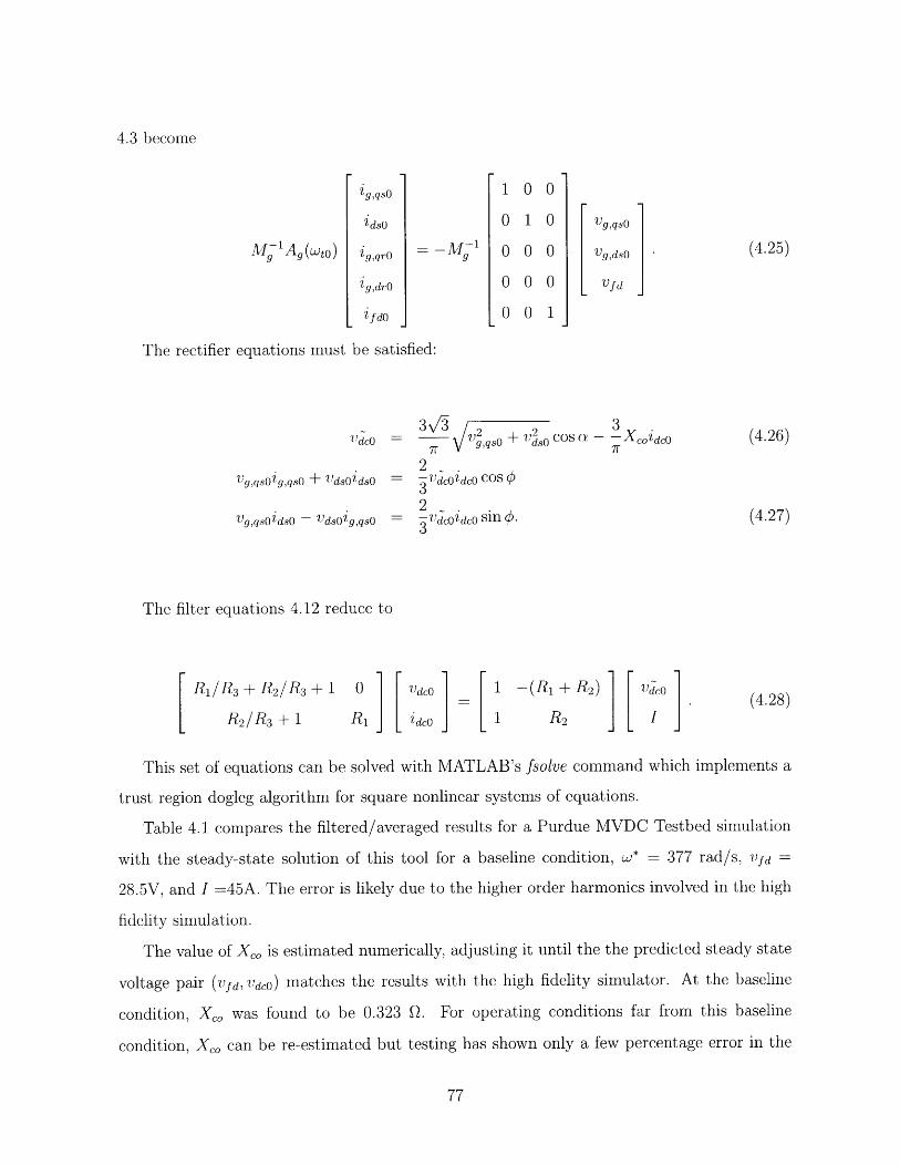
4.3 become

ig,qsO 1 0 0

'dsO 0 1 0 Vg,qso

Mg -Ag(Wto)i =g-qrO Mg 0 0 0 Vg,dsO (4.25)Zg,drO 0 0 0 Vfd

IfdO 0 0 1

The rectifier equations must be satisfied:

3 v/5 3Vico =v2 sO + vso cos a - - Xeoidco (4.26)g7r 7r

2'g,qso g,qsO + vdsO dsO = -7dco7dcO cos $

32

ogqso7 aso - VdsO7/g,qsO = vdcOidcO Sin (4.27)3

The filter equations 4.12 reduce to

R1 R + R2/R 3 + 1 0 vco ] 1-(R1+R2) Vco (4.28)R2|R3+1I R1 iaco1 R2I

This set of equations can be solved with MATLAB's fsolve command which implements a

trust region dogleg algorithm for square nonlinear systems of equations.

Table 4.1 compares the filtered/averaged results for a Purdue MVDC Testbed simulation

with the steady-state solution of this tool for a baseline condition, w* = 377 rad/s, vfd =

28.5V, and I =45A. The error is likely due to the higher order harmonics involved in the high

fidelity simulation.

The value of Xc0 is estimated numerically, adjusting it until the the predicted steady state

voltage pair (vfd, vdcO) matches the results with the high fidelity simulator. At the baseline

condition, Xco was found to be 0.323 Q. For operating conditions far from this baseline

condition, Xco can be re-estimated but testing has shown only a few percentage error in the

High Fidelity Simulation Results Steady-State Solution

VV2qs + vs 450.49 V 457.74 V

i2 ij2

,qs dg,ds 46.82 A 48.81 A

ifd 107.28 A 108.75 Avc 743.73 743.17 V

'ic 42.54 45.09 Acos # 1.000 0.982

Table 4.1: Comparison of generator side steady state solutions for analytical tool and highfidelity simulation.

steady state solution if Xc0 is held at 0.323 Q, for a variety of operating conditions.

The nonlinear nature of generator model and the power conservation constraints across

the rectifier impedes the use of traditional stability analysis methods. To overcome this,

the stability analysis is conducted about a linearized operating condition justified by small

displacement theory [43]. Let A be used to denote small displacements from the steady state.

The generator equations combined with the controlled turbine equations become:

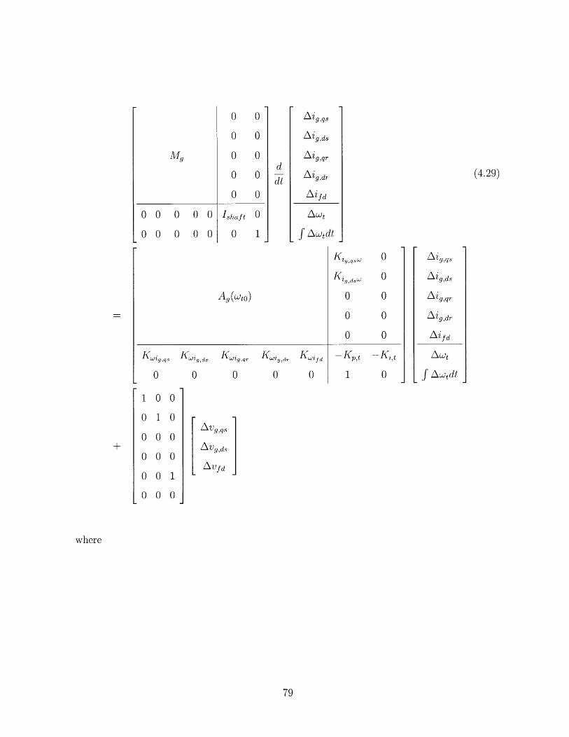
Mg

0 0 0 0 0

0 0 0 0 0

0 00 00 00 00 0

Ishaft

0

Ag(wto)

Aig,qs

Aig,ds

Aig,qr

Ai9g,d,

Aifd

Awt

f fAwtdt

0Ki dsW

0

Kwigqs Kwi ds KWigqr Kwigdr Kwifd

0 0

1 0 0

0 1 0

0 0 0

0 0 0

0 0 1

0 0 0

0 0 0

0 00 0

-K,, -Ki,

1 0

Avg,qs

Avg,ds

Avfd

(4.29)

Aig,qs

'Aig,qr

Aig,dr

Aifd

Awt

f Awdt

where

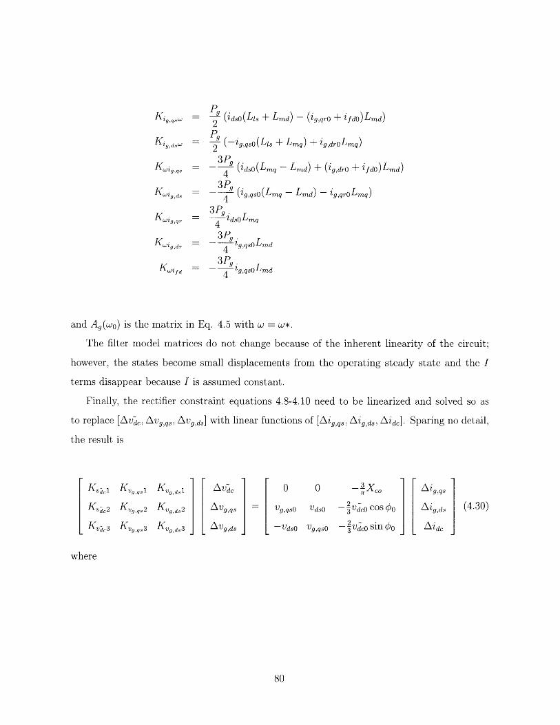
PKigqsW 2 (idso(LIs + Lmd) - (ig,qrO + If dO)Lmd)

P

K 2 (-ig,qso(Lis + Lmq) + ig,drOLmq)

3PKwgqs - - g(so(Lmq Lmd)+ (g,dro + ifdO)Lmd)

4

K3 (ig,qso(Lmq - Lmd) -igqroLmq)

3PKw isr tsoLrnq

3PgKwgdr ,qsoL

3PKWifd - ,,qsO Lmd

and Ag(wo) is the matrix in Eq. 4.5 with w = w*.

The filter model matrices do not change because of the inherent linearity of the circuit;

however, the states become small displacements from the operating steady state and the I

terms disappear because I is assumed constant.

Finally, the rectifier constraint equations 4.8-4.10 need to be linearized and solved so as

to replace [Avac, Avg,qs, Avg,ds] with linear functions of [Aig,qs, Aig,ds, Aidc). Sparing no detail,

the result is

Kvdy1 Kv9 I K9 ds 1 AlVdc 0 0 -!Xo ig,qsKv2 Kvqs2 Kv ds2 Avg,qs = Vg,qso Vd8O 2 cos po [ig,ds (4.30)

Kv , Kv Kv AV 2v~s-aoo~s - 0c sin $0 AcL wher e K0 9 J ,ds -VdsO VgqsO 3 Vdc I Jwhere

K 1 = 1

3/3V1/2K 1Vg q = 7V Vg,qso

Kv dsl 3 -1/2Vdso

4Kvdc2 2

dcO COS 00~

Kgq2 = -iqcOcos$03

Ku ~ ~ 2 2 -- gas- acvcovqeo3/2

Kvgq.2 -t..qs - 2w2 ZdcO VcO Sll'q3)VKv 27 = -gso- acvcoaop3/29 53

2 2x 2 2Kvq3 = cosin #+ 2 1idcOVdco2 sin-1(po|)/Vo

22Ko ~ ~ 3 = -ao+8 cvcosi-1(# V~sp2

Kvg,ds3 = i ws~o + idcOVcOs sin-(#lko})vso/Vo281

where

V0 1 g,qsO + 9'g,ds0

Aftersolvng tisdst ofcos( 3 VJ)

After solving this set of linear equations, substitution can be made into the generator and

filter small displacement equations and linear state space matrices can constructed. These

will be assessed in Section 4.3.

4.2.2 Motor Side Linearization

The steady state solution for the IM side is less straightfoward than the generator side because

it attempts to solve for the steady state of system with the influence of closed loop torque

control. The solution requires input values for the command torque T* and the constant DC

bus voltage Vdc. A step-by-step procedure is described here.

I Assume that at steady state the torque command is reached due to the integral control

of the torque trim controller. With this assumption, the steady state rotor speed can be

computed:

/ 2

kqo pD 5 """ = T* (4.31)( rPm)2

II With a torque signal TA;*, the AMTPA control equations are used to compute the desired

command slip frequency and stator current magnitude, w* and I*. For the first iteration,

use the guess T* = T*,.

III Then, it is assumed that the current hysteresis is such that w* and I* are attained at

steady state (in a time averaged sense), enforced by the state constaints

m,qsO + m,dsO (432)

* + Mweo - W 2 + WrmO

IV Now, with all time derivatives set to zero in Eq. 4.16, the IM steady states can be solved

for.

2 m,qsO 1

Am(Weo, WSO) mdsO 0 vm,qs (4.33)Zm,qrO 0

Lm,drO 0

where Am(oco, oso) is Eq. 4.18 computed at weo and oso.

Recall, only the q-axis stator voltage is used because the reference frame is offset such

that om,ds([) = 0 for all t. The solved value for vm,qs is the continuous time averaged value

of the actual signal.

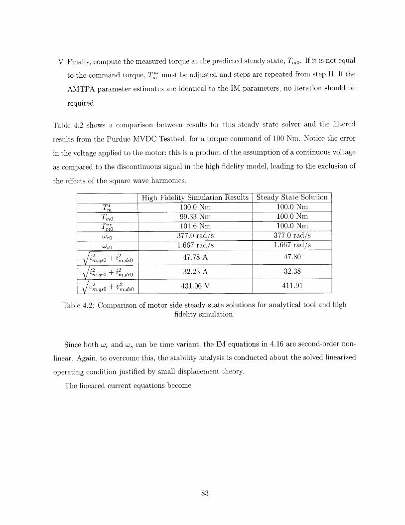
V Finally, compute the measured torque at the predicted steady state, Tmo. If it is not equal

to the command torque, T** must be adjusted and steps are repeated from step II. If the

AMTPA parameter estimates are identical to the IM parameters, no iteration should be

required.

Table 4.2 shows a comparison between results for this steady state solver and the filtered

results from the Purdue MVDC Testbed, for a torque command of 100 Nm. Notice the error

in the voltage applied to the motor; this is a product of the assumption of a continuous voltage

as compared to the discontinuous signal in the high fidelity model, leading to the exclusion of

the effects of the square wave harmonics.

High Fidelity Simulation Results Steady State Solution

T* 100.0 Nm 100.0 Nm

Tmo 99.33 Nm 100.0 Nm

T*O 101.6 Nm 100.0 NmWro 377.0 rad/s 377.0 rad/s

UsO 1.667 rad/s 1.667 rad/s2 .2

im,qsa + im,dso 47.78 A 47.80

2 *2

mqr+ m,dro 32.23 A 32.38

,s + vm,dso 431.06 V 411.91

Table 4.2: Comparison of motor side steady state solutions for analytical tool and highfidelity simulation.

Since both wr and ws can be time variant, the IM equations in 4.16 are second-order non-

linear. Again, to overcome this, the stability analysis is conducted about the solved linearized

operating condition justified by small displacement theory.

The lineared current equations become

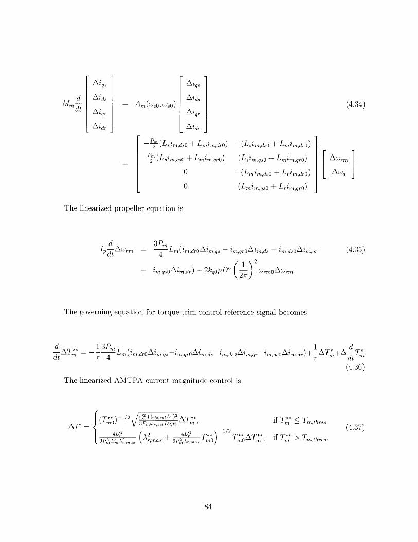
= Am(Weo, WsO)

- s Lim,aso + Lmim,drO)

-(Lsim,so + Lmimqro)

0

0

-(Lsim,dsO + Lmim,drO)

(Lsim,qso + Lmimqro)

-(Lmim,dsO + Lrim,drO)

(Lmim,qso + Lrimqro)

The linearized propeller equation is

3Pm

4 Lm(im,'roAim,qs - im,qroAim,ds - im,dsOAZm,qr

+ im,qsoAim,cr) - 2 kqoPD 5 o)2 WrmoAwrm.27r

The governing equation for torque trim control reference signal becomes

d 1 3P 1 dAT m Lm(im,droAim,qs - im,qroAim,ds -im,dsOhim,qr+2m,qsOAim,dr)+- AT*+AT*dt m T4 T m dt m

(4.36)

The linearized AMTPA current magnitude control is

(T**|-/2AI* = o

9 L\29P,,2 L'M A2ma

7- (ssetL~I)2

3Pmws,sctLr m

max 9 p94 2m no)

if T* * Tmthres

TnoAT*, if T* > Tm,thres-

dM

Aiqs

Aids

Aqr

Adr

Aiqs

Aids

Aiqr

Aidr

(4.34)

AwrmAw

dtIpdt m (4.35)

(4.37)

0,TAw*

32r. T*I PAr,mo £

if T*:* < Tm,thres

if T*;* > Tm,thres-

4.3 Open Loop Analysis

In this section, the linearized equations are combined to create open loop state space matrices

for both the generator and motor sides. Analytical transfer functions, G(s) = C(sI - A)-1B,

are visualized with Bode magnitude plots. For comparison, frequency response plots have

been attained from high fidelity simulation at discrete frequencies.

4.3.1 Generator Side Open Loop Analysis

Equations 4.29 and 4.30 can be combined with the linearized version of Eq. 4.11 to produce

a linear state space model for the generator side:

dAx

x = g,qs

- Ag,oiAx + Bg,ozAu

i 9 ,ds i,qr igdr ig,f5d W f wtt Vdc Vdc Vdc

(4.39)

Vdc idc (4.40)

where o) denotes the ith time derivative of the bus voltage.

and

(4.38)

y = C,,Ax

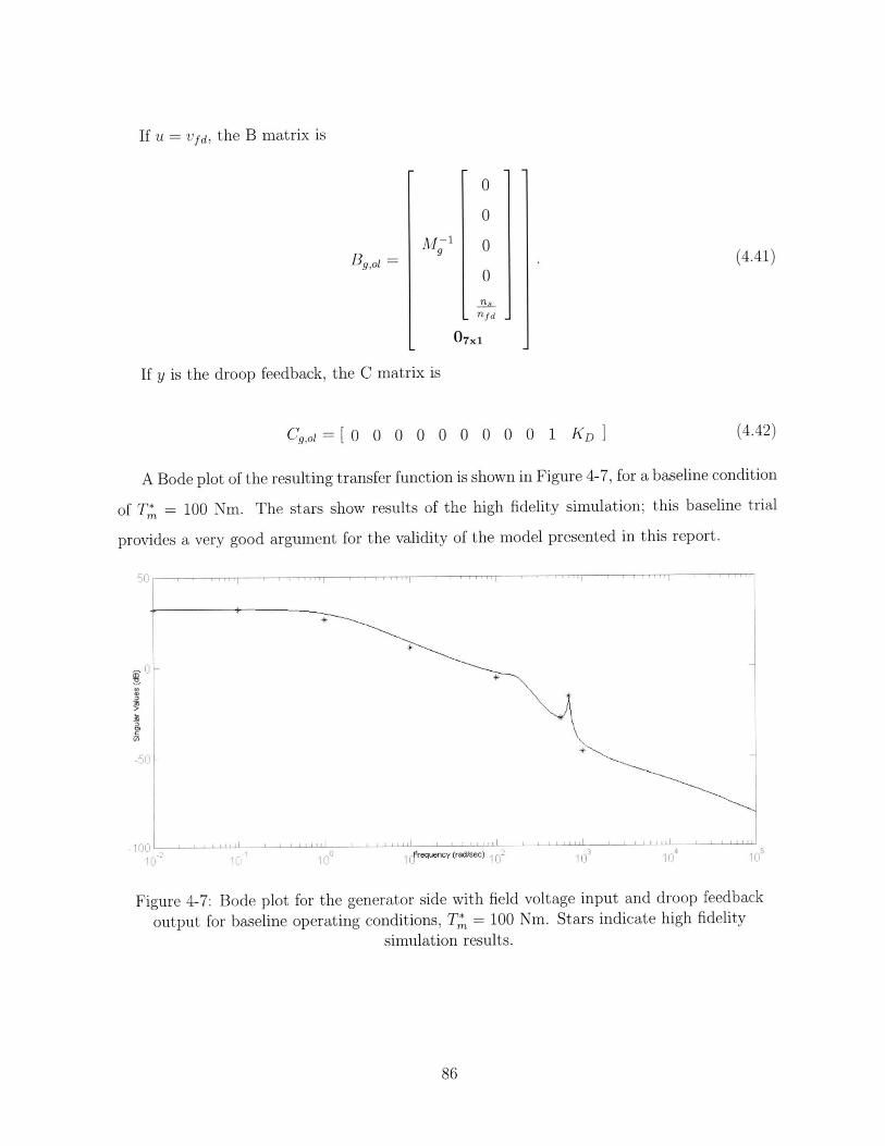
If u = Vf, the B matrix is

Bg,o=

If y is the droop feedback, the C matrix is

C9,01 = [ 0 0 0 0 0 0 0 0 0 1 KD

A Bode plot of the resulting transfer function is shown in Figure 4-7, for a baseline condition

of T*, = 100 Nm. The stars show results of the high fidelity simulation; this baseline trial

provides a very good argument for the validity of the model presented in this report.

1 i~Jfrequency (rad/sec)

Figure 4-7: Bode plot for the generator side with field voltage input and droop feedbackoutput for baseline operating conditions, T = 100 Nm. Stars indicate high fidelity

simulation results.

0

0

0

0

0 7x1

(4.41)

(4.42)

V)

4.3.2 Motor Side Open Loop Analysis

Equations 4.34 and 4.35 can be combined to produce a linear state space model for the motor

side when the torque command does not exceed the torque threshold. When the torque

threshold is exceeded, Equations 4.36 and 4.38 must be incorporated to include the dynamics

of the IM slip frequency. The general linear state space model is

dAx= Am,oiAx + Bm,oAuAdt

(4.43)

Y = Cm,oiA.

where u is the the stator voltage magnitude and y is the current magnitude feedback.

When T,:* < Tm,thres, the states are x =[ imqs im,ds m,qr m,dr Wrm ] and the A matrix

is

Am,oi =

Mm

0 0 0 0

0

0

0

0

Ip

(4.44)

Am(oeo, WsO)

3PmLm 3 m,qr0 - -3 m,ds 3PmLm m qs04 '- m,drO 4Pmmq 43PmL s 4 Zm,qsO

- Pm (Ldimd- + Lmim,drO)

P (Lsim,qsa + Lmim,qro)

0

0

~2kqopD )2mo

The B matrix for the input Avm,q, is

Bm,o =[Mm

0 0 0 0

The feedback for the system is the magnitude of the stator current + iM,ds For the

linearized system, the open loop C matrix is Cm,ol = (i*m,qs0 + i im,ds 0 0 0].

When T** > T.,thres, a state is added for the trim control, T*. The A matrix is

0 0- ~Mm 00

Am,oiz = 0010 0 0 0 Ip 0.0 0 0 0 0 -r .

(4.46)

(Lsim,aso+Lmim,dro) -32 (Leim,ado+Lmim,dO)3Pm r,max

Am (weo,wso)

3 Pm Lm,4 im,drO

3Pm LmL 4 im,drO

3Pm Lm ir

3Pm LmSim,qrO

3PmLm. 3PmLM in- mim,dsO 3 L m,qsO

3iPmim 3 Pm Ln4 imdsO 4 im,qsO

P (L 8 im,qso+Lmim,qro)

0

0

2kqopD5(, 2w'. 0

3 2 -' (L im qso+Lmim,qro)Zr3Pmr,max

-Pm 2

(Lmimaso+LFimdaro)

2r L +zu (Lmim,qso+Lrim,qro)3P A,max

Assuming that the torque command T, is held constant, the B matrix is only augmented

by one zero

Bm,o=

Mm

0 0 0 0 I, 00 0 0 0 0 r

1

0

0

0

0

0

(4.47)

0

0

0

0

I,

(4.45)

The C matrix in augmented with one zero C.,ol (iMqso + it'a 5 o /[mqs im,ds 0 0 0 0].

:5~ 1:

Us

:5

<H

Frequency (rad/sec)

Figure 4-8: Bode plot for motor-propeller with stator voltage input and stator currentmagnitude feedback for the output, for a 100 Nm operating condition. Stars indicate Purdue

MVDC Testbed model results.

For validation purposes, a Bode plot is shown in Figure 4.3.2 for the operating point open

loop transfer function, for a baseline torque command of 100 Nm. Figure 4.3.2 shows the

results for a torque command of 200 Nm. Notice that the five state model does not capture

the frequency domain behavior exactly when operating above the torque command threshold.

4.4 Closed Loop Analysis

This section investigates methods for closed loop analysis of the generator and motor sides.

Generator analysis is trivial due to its PI compensation. The motor side deserves more atten-

tion due to its more complex compensator. One method is introduced for this analysis.

4.4.1 Generator Side Closed Loop Analysis

In the case of PI control, the closed loop A matrix becomes [33]

Aci = [Ag,o - Bg,oiKp,vC,oi B, 01K,

- Cg,01 0(4.48)

6 State Model5 State Model1

10 0 Frequency (rad/sec) 10 10 0

Figure 4-9: Bode plot for motor-propeller with stator voltage input and stator currentmagnitude feedback for the output, for a 200 Nm operating condition. Stars stars indicate

Purdue MVDC Testbed model results.

where K,,, and Ki,, are the droop gains.

Note that this representation introduces a new state derivative to the system: the integral

of the feedback combination. This can be used to inspect the poles of the closed loop system.

As an example of frequency domain analysis, one can examine the closed loop command

following transfer function H(s) = K(s)G(s)/(1 + K(s)G(s)), where K(s) is the compensator

transfer function. The classic PI compensator, K(s) = KPsS+K , is the default for the Purdue

MVDC Testbed droop control.

For more results, see [64].

4.4.2 Motor Side Closed Loop Analysis

Methods for the closed loop analysis of the motor side require a more novel approach due to

the hysteretic relays in the control loop. The three phase current hysteresis control is shown

in Figure 4-10.

The three phase control problem is intractable for several reasons, the primary of which

is that the open loop model was developed in the dq reference frame. Instead, a generalized

combined phase, or current magnitude, hysteresis control will be used in place of the three

phase control, see Figure 4-11. The current magnitude is the feedback from the open loop

Figure 4-10: Three phase hysteresis current control for IM torque management.

Figure 4-11: A generalized combined phase hysteresis control.

models developed in the previous section, the voltage magnitude is simply Vm,q, because of

how the rotating reference frame was defined in Section 4.1. This approximation may not

capture all of the dynamics of the three phase compensation, but it is used here as a starting

point.

The combined phase feedback model falls into the control theory category of sliding mode

control [39]. Work during this thesis and other studies have shown that traditional describing

function methods [27], with their first order approximations, are not reliable for for this type

of compensation [17]. Two methods are presented in [64] for analysis of this system type.

Here, only one is developed.

"The classical approach to analysing the closed-loop response of a system under sliding-

mode control is to seek a smooth control law that approximates the effects of the rapidly

switching control observed under digital implementation" [12]. Several different approaches

can be taken to attain the equivalent control law. In the method presented here, Vmqs is

instantaneously set to the value predicted by the inverse steady IM equations, to satisfy a

torque command of T!*. This is a continuous analog to the rapid adjustment being made

by the hysteresis control to keep the current states near their target. Mathematically, this is

stated

Vm,qs

0

0

02 +im

tm qs m ,ds

= Am

im,qs

im,qr

im,dr

(4.49)

= 8T*,*.

where - /+w"2 )3PmwL$mrr

After solving for om,qs and linearizing with small displacements, the result when T* <

Tm,thres is

Avm,qs - [Kis - LS( Prmo2 + Ws,set)1 Aim,ds +

+P (m

2 s Lem,dso

Lm rm o+ Ws,set)] Aim,dr

+ Lm rn,drO)j AWr + KTAT :

where

Kis = srm,dsO(@oT*n* - imdso) 1/2 (4.51)

KT = - (T ,dSo)

and 8 0 is 0 such that w, -- os,set.

When T,*5 > Tm,thres, the equation for Avm,q, accounts for the changing slip frequency:

(4.50)

P PMAvm,qs [Kids - L(P rmo + wso)l Aim,ds + [-Lm( wrm 0 + W80) Aim,dr (4.52)

PM+ P (LsimdsO + LmzmdrO)1 AWrm + KTAT :

2

where

r~a2 + * 0T *2 -1/2

K1) 1/2 (4.53)Kids rs *m,iso( L2 mO mdsOm

KT + 0 A2 + 2 )1/2 _ 2r_-rS81( m* _ Im,dsO) 122 (Lsim,dsO + Lmim,drO)

mn 3mr,max

2L /4

and 0-1 = o ,--an ~ 9LIP/jArmax~

With Avmqs as a linear function of the other states, one can substitute it into Eq. 4.43 to

attain a closed loop A matrix. For closed loop system analysis, the T** state is required so

the open loop A matrix in Eq. 4.46 is used. When T** < Tm,thres the entries the 6th column

must be removed because the slip frequency is held constant.

The closed loop B matrix allows for the input of torque command Bm,ci = [0 0 0 0 0 1]'.

Notice that the trim control described in Eq. 4.21 has torque command input -T +

The closed loop C matrix gives output for the measured torque

Cm,ci = 4Lm [ im,dO -m,qrO -- im,dsO im,s0 .

Finally, for the sake of validation, results are given in Figure 4.4.2 for the closed loop

transfer function, at T, =100 Nm, for two different trim control gains. Results are shown for

the high fidelity simulation where the three phase current hysteresis control was replaced with

combined current hysteresis. The lack of fidelity at higher frequencies was expected because of

the use of a continuous control law in place of the ON/OFF switching, for analysis purposes.

The results seem to correspond intimately up to and beyond the cutoff frequency, so at the

very least a command following design tool has been provided.

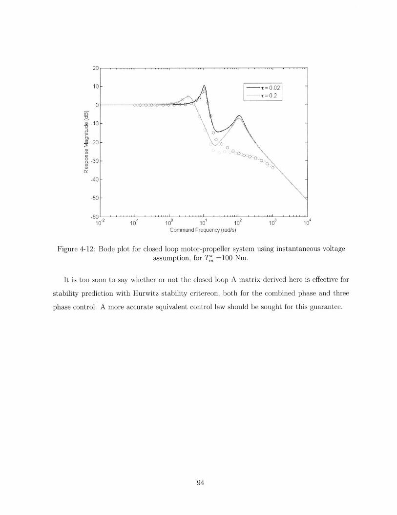
2 0 . . . . . . . ..

10- 1=0.02--10 -

O. -30 --

-40 --

-50 -

-60 - '10 10 10 10 10 10 10

Command Frequency (rad/s)

Figure 4-12: Bode plot for closed loop motor-propeller system using instantaneous voltageassumption, for T* =100 Nm.

MC

It is too soon to say whether or not the closed loop A matrix derived here is effective for

stability prediction with Hurwitz stability critereon, both for the combined phase and three

phase control. A more accurate equivalent control law should be sought for this guarantee.

Chapter 5

Simulation Results with AES Model

In this chapter, the capacity of this AES simulator is demonstrated with simulation experi-

ments. Many of the examples shown are straightfoward, for deterministic instances, and are

meant for verification of the system model as much as for demonstration of capability. In

Section 5.1, power conservation of the IPS during ship startup in shown. In Sections 5.2 and

5.3 simulations for maneuvering in calm seas and random seas, respectively, are carried out.

Section 5.4, explores the some statistical behaviors of the AES using Monte Carlo simula-

tion techniques.

In this chapter, the full scale DDG-type AES model, as depicted in 2-1, is used. The

operation scheme for the prime movers is to share the power loads equally; this is an inefficient

scheme, but it does not detract from the demonstrative results given. The baseline parameters,

mechanical and electrical, are given in Tables 5.1-5.5 for the sake of repeatability. A DDG51

offset was used for the seakeeping model with bilge keel data. 38MW motors are used with

parameters defined in Table 2.1. All parameters are adjustable via an input file in the AES

simulator.

Displaced Mass Propeller Diameter Wetted Aream=7e6 [kg] D=4.5 [m] AW=5200 [im 2 ]

Wake Fraction Thrust Coefficient Pitch RatioW= 0.1 t=0.1 P/D=1.0 [ ]

Propeller Shaft Moment of Inertia Hull Drag Coefficient Fluid Density

1m=1.33e5 [kg - m2] Cr=3e-3 p=1025 [kg/m 3]

Table 5.1: Ship surge parameters taken from DDG51 information or [60].

LFull Locking Torque No Load Speed Turbine Shaft Moment of InertiaQlok=1 23 [kN-m] nt,max= 6 8 75 [rpm] It=400 [kg - m2

Table 5.2: Gas turbine parameters chosen to represent GE's LM2500 [26].

Stator Resistance Stator Inductance Mutual Inductance Pole NumberRg=2 .2 7e-2 [Q] Lg=0.391 [mH] Mg=18.0 [mH] P9 =2

Table 5.3: SM parameters selected to provide 4160 V-1 for a rotor speed of 60 Hz.DC Bus Capacitance Notching Resistance

C=0.037 [F] Rp=.05 [Q]

Table 5.4: Rectifier/inverter parameters. Capacitor sized to store the peak capacity of thepower plant for one cycle of the fundamental frequency.

Ship Length COG to Rudder Rudder Face AreaL.=180.0 [m] xP=75.0 [m] Ar=20.0 [m 2]

Rudder Lift Coefficient Rudder Drag Coefficient Rudder Swing RateCL=3-31 [] CD046 I Ar=0.1 [rad/s]

Table 5.5: Maneuvering parameters for DDG-type ship. Rudder parameters informed by [42].

5.1 Conservation of Power across IPS

In this section, power conservation across the IPS is demonstrated in an attempt to validate

the system model. The trial presented is a startup from idle to 25 knots, in calm seas. The

nonlinear maneuvering model is not used here because its accuracy is compromised below

its speed of linearization, approximately 22 knots. Instead, the translational surge model

presented in 2.16 is employed.

Power is inventoried at the output of the turbines, the SMs, the inverters, the IMs, and the

ship hull. The equations for these powers are given in Table 5.6 using notation from Chapter

2.

Turbine Generator Inverter Motor Ship

n=4 n=4 n=2 n=2 n=127rQtnt 3Re {Eai*} S 3Re {Vmin} 5 2IrQmn, > R8 u

Table 5.6: Power equations.

Figure 5-1 shows the time evolution of the propeller speed and ship speed during startup.

E 300

200 -

0

C

O 20 30 40 50 60 70 80 90 100

20-

CDCD

S 0 -------- I

20 30 40 50 60 70 80 90 100 110 120Time (s)

Figure 5-1: Time evolution of propeller speed and ship speed for startup.

The most notable characteristic is that the propeller speed at 25 knots is approximately 225

rpm (and can be shown to be approximately 300 rpm at full-ahead). While the motor selected

is rated for rotor speeds up to 300 rpm, these speeds are rather large for conventional marine

propellers and could lead to significant cavitation. Propeller diameter is likely to be larger

than 4.5 m, as used in this simulation, to achieve full-ahead at lower propeller speeds.

Figure 5-2 shows the time evolution of the inventoried power outputs, during startup.

Table 5.7 shows the efficiency of the different componentry at steady conditions. As expected,

high efficiency is observed through the IPS. The efficiency of the generator varies between

95 % and 97 % near rated conditions but drops off for lower power generation. The power

electronic efficiencies are around 99 %. The IM efficiency seems rather large; traditionally one

would expect 3-5 % loss. However, motors of this magnitude, 38 MW, should be even less

lossy than conventional propulsion motors - by how much is a question for those researching

the development of these high power IMs. TIm in Eq. 2.5 can be altered to reflect other losses

such as friction.

The propeller used is 70 % efficient at steady state; this could perhaps be improved with

a higher pitch ratio or an innovative propeller design.

Not shown are the turbine thermal efficiencies because the model does not have capability

to predict them accurately. From practice, it is expected that the efficiencies would improve

8011

70- Turbine Output

60 - Generator OutputInverter Output

50 - Motor OutputShip Output

40-

o 30-

20-

10-

020 30 40 50 60 70 80 90 100 110 120

Time (s)

Figure 5-2: Power outputs for different components in AES for startup.

20 knots 25 knots 30 knots

Synchronous Generator 0.909 0.950 0.971Power Electronics 0.991 0.992 0.988Induction Motor 0.993 0.992 0.991

Propeller 0.705 0.703 0.702

Table 5.7: Efficiencies of AES components for different operating conditions.

to as high as 37 % as their rated power (21.5 MW) is approached and would drop off to about

28 % at half the rated power [53].

5.2 IPS Performance during Routine Maneuvering

In this section, maneuvering trials and the corresponding effects on the bus voltage and prime

mover speed are examined. The trials are purposefully tutorial to clearly demonstrate the

type of studies that can be achieved with the AES simulator. Three fundamental maneuvers

will be studied and discussed in this section: acceleration, braking, and heading changes.

Other hydrodynamic results for this maneuvering model are given in [51] for those readers

interested. The section concludes with a demonstration of second order forces and their effect

on maneuvering and fuel consumption.

................. ............

5.2.1 Acceleration

Here, employing the nonlinear maneuvering model from Section 2.4, is a computational study

involving the acceleration of the notional AES from 25 knots to full-ahead using a step com-

mand. The resulting propeller and ship speed are shown in 5-3. Notice that the motor operates

at speeds beyond its rated speed, 300 rpm; the propellers would need to be resized or given a

higher pitch ratio.

320

a.

300-

280-

24

50 200 250 300 350

30 -

C 29 -

'2-S 0 5 0 5

Time (s)

Figure 5-3: Time evolution of propeller speed and ship speed for acceleration fromapproximately 25 knots to full-ahead.

Figure 5-4 shows the effect of the acceleration on the bus voltage and the prime mover.

As the motor demands more power, the prime mover is subject to more emf torque from the

generator, it slows down and in effect the bus voltage is reduced. With the baseline controls,

the gas turbine sustains an approximately 20 % loss of speed and operates away from its

rated speed for approximately 20 seconds. The field control of the bus voltage acts slightly to

mitigate voltage drop (without independent control, one would expect the p.u. DC voltage to

be identical to the p.u. turbine speed)

Figure 5-5 shows the bus voltage and turbine speed for a different set of field voltage

control gains. Still, this is not a satisfactory design. An interesting problem is the joint

optimal control of the turbine throttle and field voltage.

CD

1

0

.90 200 210 220 230 240 250

Time (s)

Figure 5-4: Per unit bus voltage and turbine speed during accelerationKi,V=0.0005).

(K,=0.0001 and

1.3CD

1.2

1.1

S1

0.90.

200 210 220 230 240 250 260 2'

1.4

0.8

.190 200 210 220 230

Time (s)240 250 260 270

Figure 5-5: Per unit bus voltage and turbine speed during acceleration for higher gains(Kp,=0.0003 and Ki,v=0.001).

5.2.2 AC Braking

AES braking can be accomplished by 1) switching off power to the IM and coasting, 2) locking

the motor to increase drag, 3) AC braking and 4) crashback. The AC braking and crashback

procedures spell the largest demands for the IPS. In crashback, the IM is brought to zero speed

and then reversed; this requires a control protocol more sophisticated than volts per Hertz

and is not implemented here. In AC braking, the IM, or more generally the asynchronous

machine, is excited with negative slip such that it behaves like a generator. In effect, the ships

translational power is converted back to electrical power, much like a water turbine, and the

emf torque acts to slow the propeller. The energy that gets forced back into the drive system

100

0

-

.

must be stored, for instance by capacitors or flywheels, or dissipated. The management and

possible harvesting of this braking energy is an important problem in AES design.

To conduct this type of simulation, small alterations were required for the propeller and

IM models. First, a propeller model was required that gave thrust and torque coefficients

at large advance coefficients where torque and thrust reverse directions. Rubis's empirical

four-quadrant model provides this [60]. Also, an offset discontinuity was inserted to prevent

the singularity that occurs at zero slip with the equivalent circuit IM model.

The propeller speed and ship speed are shown in Figure 5-6 for the AC braking procedure.

Water brakes are likely to be used at lower speeds to bring the ship to a complete halt.

- 200EEL

150 -

- 100-

-

50-0.0

200 250 300 350 400 450 500

0200 25 30 5 0 5 0

Time (s)

Figure 5-6: Propeller and ship speed during AC braking.

The following is a description of the power transients in the IPS during the AC braking

procedure. First, the induction machines generate electrical power and it flows back into the

IPS and congregates in the capacitors. Immediately after braking, the IM demands no further

energy, so the energy is stuck in the IPS and must be dissipated or stored. In the ideal case,

switching is used to open up exigency loads to expire the excess energy and buffer the prime

movers from the power surge, and with no major loads to service, the prime movers reduce

their throttle to idling. Figure 5-7 shows an example of the bus voltage and turbine speed

perturbations during AC braking in ideal power management. These are acceptably controlled

responses but bear in mind that the "ideal" power management for the AES requires the

containment or dissipation of most of the ship's kinetic energy, about 10 MJ in each power

101

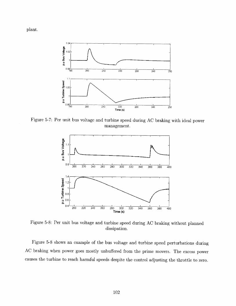
1.

D)

("L0.

200 210 220Time (s)

230 240 250

Figure 5-7: Per unit bus voltage

0)CM

0L

and turbine speed during ACmanagement.

braking with ideal power

1.4CD0) 1.2-C).12e 1

-2 0.8-I-2 0.6--

0.0.4

200 220 240 260 280 300 320 340 360 380 4CTime (s)

Figure 5-8: Per unit bus voltage and turbine speed during ACdissipation.

braking without planned

Figure 5-8 shows an example of the bus voltage and turbine speed perturbations during

AC braking when power goes mostly unbuffered from the prime movers. The excess power

causes the turbine to reach harmful speeds despite the control adjusting the throttle to zero.

102

plant.

0 200 210 220 230 240 250

-

O 1.05

-

CLa05190

1.1

200 220 240 260 280 300 320 340 360 380 4

04

02

000

2500------ 450 Command

- - - 904 Command2000-

1500 -

0 1000-

500-

0

3000 3500 4000 4500 5000 5500 6000 6500Global X (m)

Figure 5-9: Global positions for heading change trials with 450 and 90' commands.

5.2.3 Heading Changes

Turning at high speeds can have a profound effects on the IPS that must be managed. First,

while making a turn, the ship becomes less streamlined in its direction of travel and more

power is required to keep it up to speed. Secondly, the propeller operation is altered due to

changes in the axial and traverse inflow. Both at the onset and egress of the turn, these cause

load fluctuations that are of concern to IPS operation.

Figure 5-9 shows the global position of a ship for a 45' and 90' heading change. The

trajectories match well with theory.

Figure 5-10 demonstrates the two key effects relevant to propulsion management that occur

when making a turn. The first subfigure shows the increase in required power to maintain

speed. For the 45' turn there is approximately a 6 % increase in required power and for the

90' turn there is approximately a 15 % increase in required power. In the second subfigure,

the loss of propeller efficiency due to altered inflow velocity is demonstrated.

5.2.4 Second Order Forces

Figure 5-11 shows the maneuvering states for simulations in sea state 3 (SS3) and state

state 6 (SS6) to illustrate the effects of the added resistance and drift forces. These effects

are essential in ship design, for example, in assessing fuel consumption or designing global

103

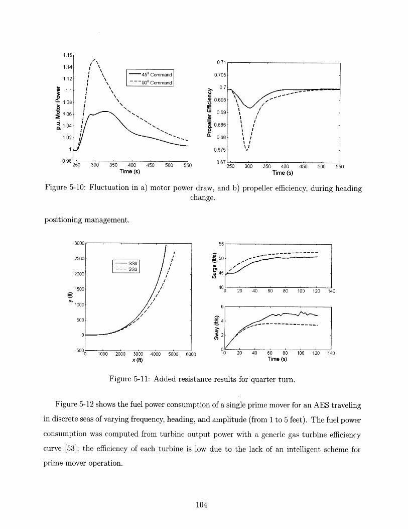
1.160

1.14\

1.12 - 450 Command 0.70590 Command

1.08-

1.06

1.04 -- 80.

1.02 0.69

1 0.675

250 300 350 400 450 500 550 - 250 300 350 400 450 500 550Time (s) Time (s)

Figure 5-10: Fluctuation in a) motor power draw, and b) propeller efficiency, during headingchange.

positioning management.

3000- 55

2500- 50--

2000 45

1500 400 20 40 60 80 100 120 140

1000 -6

500 4

0 3

0 1000 2000 3000 4000 5000 6000 0 20 40 60 80 100 120 140

x (ft) Time (s)

Figure 5-11: Added resistance results for quarter turn.

Figure 5-12 shows the fuel power consumption of a single prime mover for an AES traveling

in discrete seas of varying frequency, heading, and amplitude (from 1 to 5 feet). The fuel power

consumption was computed from turbine output power with a generic gas turbine efficiency

curve [53]; the efficiency of each turbine is low due to the lack of an intelligent scheme for

prime mover operation.

104

,.5.6-

E 5.4- - Head Seas-45' Bow Seas

O 5.2-

05 -

4.6-

440 0.5 1 1.5Wave Frequency (rad/s)

Figure 5-12: Fuel power consumption for travel in discrete seas of amplitude varying from 1to 5 ft, for bow and head sea travel.

5.3 IPS Performance in Random Sea Environments

This section examines the coupling between seakeeping and the IPS. While this can occur

due to lateral movement of and wave interaction with the propeller, focus here is on surface

effects, like cavitation and out-of-water conditions. The models for these losses are discussed

in Section 2.3. A static hub distance ho of 6.0 meters is selected for these trials, informed

by [42].

Surface effects among other things result in rapid losses in propeller loading followed by

rapid load recovery at reemergence. For traditional propulsion systems, this poses less of a

problem due to the large inertia of the drive system. For the electrical drive, the unloading

would theoretically result in rapid acceleration of the rotor and potentially large power tran-

sients. This is imagined as one of the most challenging problems when conceptualizing the

distribution and IM controls.

As seakeeping involves a random wave process, the analysis should factor in uncertainty

quantification to understand the average behaviors and the bounded behaviors of surface

effects. This will be addressed in Section 5.4. In the present section, results of single instance

simulations are provided and discussed to clearly show the utilities of this AES simulator. The

first subsection examines travel in head seas. The second subsection examines the execution

of 3600 turn.

105

.................. ... .... . ....... .... :::: ..........

5.3.1 Seakeeping in Head Seas

This simulation in head seas is for a DDG51 type hull shape with a target ship speed of 25

knots, in SS6. Results are shown for 80 seconds, or approximately 6 fundamental wave periods

(defined as the period of the peak frequency in the spectrum). Figure 5-13 shows the wave

height at the stern and the distance from the propeller hub to the mean water line. Figure

5-14 shows the h/R plot and the corresponding thrust and torque losses. Figure 5-15 shows

the propeller speed and the corresponding per unit power transients at the IM, where the

normalizing IM power is that which gives steady 25 knots operation with a fully submerged

propeller.

In these results very frequent cavitation and occasional emergence are observed. In the

cases of emergence, only a small fraction of the propeller comes out of the water. Note: in

higher seas states, it is possible to see the majority of the propeller come out of the water

resulting nearly in a no load condition on the IM that can be especially harmful; these higher

sea states are not simulated here because linear seakeeping approximations in high sea states

tends to lose accuracy.

With the specific parameters chosen, a 50 rpm propeller speed perturbation and a 25 %

IM power pertubration are observed. If operating at full-ahead, these transients would result

in the exceeding of IM limitations.

5.3.2 Seakeeping during 360 Degree Maneuver

This section presents results for the simulation of an AES completing a 3600 turn in SS6, with

a ship speed command of 25 knots, beginning in head seas. The turn is achieved by sending

a ramp command to the heading control; the slope of the ramp command is set so that the

rudder reaches its maximum angle before stall. Figure 5-16 shows the birds eye view of the

ship executing the turn; time markers are given so that heading information can be deduced

when viewing the time evolution plots. The radius of the turn is approximately three ship

lengths. This is about what one would expect from a DDG type ship at 25 knots [42].

Figure 5-17 shows the h/R evolution during the maneuver with domains indicating cav-

itation, propeller out of water, and hub out of water conditions. This shows that head seas

tend to be the most threatening to load perturbation. In following seas at 25 knots, the ship

106

40

-110 20 30 40 50 60 70 80 90Time (s)

Figure 5-13: The wave height and propeller height at the stern during seakeeping in headseas.

10 20 30 40 50 60 70 80 90

---- ,p,11PQ VVi LI Lit! V-10 20 30 40 50 60 70 80 90

Time (s)

Figure 5-14: The h/R plot (top) and the propeller losses (bottom) during seakeeping in headseas.

S260-0

0.CO 240-

O 220o 010 20 30 40 50 60 70 80 900.

1.3 1 1

13

0.9 L10 20 30 40 50 60 70 80 90

Time (s)

Figure 5-15: The propeller speed (top) and the IM power transients (bottom) duringseakeeping in head seas.

107

1

- 0.8

0.60

0.4

0L

I

400

-200 L-UU b

2500 3000 3500 4000x (M)

Figure 5-16: Global position of ship during full turn.

is excited very little in heave and pitch.

Figure 5-18 shows the propeller and ship speeds during the maneuver. To maintain 25

knots during the low radius turn, approximately 255 rpm are required with transients leading

to speeds upwards of 300 rpm. This exceeds the rated speed for the motor is is likely to lead

to damage or inefficiency. Note also that in addition to the haphazard seakeeping motions,

the thrust transients leads to rapid 2-3 % changes in surge speed, which may or may not be

perceptible onboard.

Figure 5-19 shows the per unit IM power during the maneuver. To keep up to 25 knots

during the turn, about 160 % of the unit motor power is required with transients exceeding

200 % of the unit power requirement.

5.4 Stochastic Simulation with AES Simulator

The examples given in the previous sections serve as system model validation, but they do

not get at the heart of the AES simulator's utilities. The AES simulator has been run in

under real time on the author's Dell M1530 laptop, programmed in MATLAB and Simulink,

and run with Simulink's Rapid Accelerator mode [501. The speed of the simulator makes it a

likely candidate for studies requiring iterations. Here, as an example, high effort Monte Carlo

108

I I I I I I I

20 2 0Propeller O of WaterI

I ~ i lfiHub OtofWater 40

100 150 200 250 300 350 400 450 5Time (s)

Figure 5-17: h/R plot during 360' turn.

Time (s)

Figure 5-18: Propeller speed (top) and ship speed (bottom) during 3600 turn.

2.51

0a -

:i 1.5 --

200 250 300 350 400 450 500Time (s)

Figure 5-19: p.u. IM power during 360' turn.

109

W dkoW .I . I

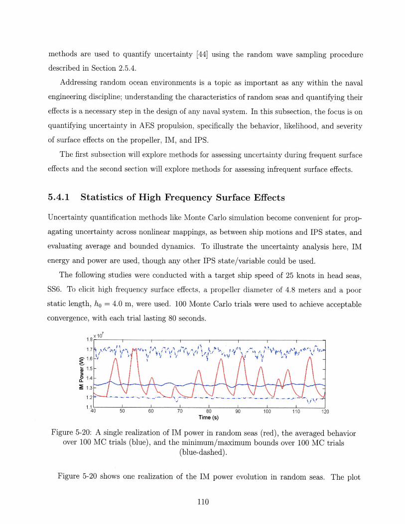
methods are used to quantify uncertainty [44] using the random wave sampling procedure

described in Section 2.5.4.

Addressing random ocean environments is a topic as important as any within the naval

engineering discipline; understanding the characteristics of random seas and quantifying their

effects is a necessary step in the design of any naval system. In this subsection, the focus is on

quantifying uncertainty in AES propulsion, specifically the behavior, likelihood, and severity

of surface effects on the propeller, IM, and IPS.

The first subsection will explore methods for assessing uncertainty during frequent surface

effects and the second section will explore methods for assessing infrequent surface effects.

5.4.1 Statistics of High Frequency Surface Effects

Uncertainty quantification methods like Monte Carlo simulation become convenient for prop-

agating uncertainty across nonlinear mappings, as between ship motions and IPS states, and

evaluating average and bounded dynamics. To illustrate the uncertainty analysis here, IM

energy and power are used, though any other IPS state/variable could be used.

The following studies were conducted with a target ship speed of 25 knots in head seas,

SS6. To elicit high frequency surface effects, a propeller diameter of 4.8 meters and a poor

static length, ho = 4.0 m, were used. 100 Monte Carlo trials were used to achieve acceptable

convergence, with each trial lasting 80 seconds.

x 101.8

1.5-

1.3-

11 40 50 60 70 80 90 100 110 120

Time (s)

Figure 5-20: A single realization of IM power in random seas (red), the averaged behaviorover 100 MC trials (blue), and the minimum/maximum bounds over 100 MC trials

(blue-dashed).

Figure 5-20 shows one realization of the IM power evolution in random seas. The plot

110

#_ - - ... ..................... ............... __ - -1 k _: .

35

30-

25-

20-

15-

10-

5-

1.1 1.2 1.3 1.4 1.5 1.6 1.7 1.8IM Power at t=100 s () x 107

Figure 5-21: Histogram of IM power at t=100 s.

90 10 110Excess Energy (MJ)

140

Figure 5-22: Histogram of excess power due to propellerhead seas, SS6.

emergence for 80 seconds travel in

also includes the average value and the maximum and minimum values observed over the

100 simulations. Standard deviations were not used to define the bounds as the instanta-

neous probability distribution function (pdf) for any given time is heavily skewed toward the

minimum; this is illustrated in Figure 5-21, a histogram of IM power values at t=100 s.

Figure 5-22 shows a histogram of the excess energy drawn by one of the IMs due to propeller

emergence, over the entire 80 second simulation. As expected by the central limit theorem,

the pdf looks to have a normal distribution. The average excess energy is approximately

94.1 ± 33.3 MJ, or the average excess power drawn by the IM is 1.18 MW.

Another approach is to look at the spectral content of the power transients. Welch's method

was used to produce the periodogram in Figure 5-23 [72]. Again, maximas and minimas over

111

7X10

6-

I \

N 5---- Average Spectral Density

- - Maximum Spectral Density4 - Minimum Spectral Density

3-

0 02 04 06 08 1 1.2 1 4 1.6 1.8 2IM Power Signal Frequency (rad/s)

Figure 5-23: Periodogram illustrating the spectral content of the IM power transients during25 knots travel in head seas, SS6.

the 100 trails were used to illustrate the bounded behavior. This periodiogram can be used

to predict statistical moments and furthermore occurrence rates. There will be more on this

in the next subsection.

5.4.2 Statistics of Low Frequency Surface Effects

In the case of high frequency surface effects, the analysis focused on wave forms and their

statistical behavior. In the case of low frequency surface effects, the analysis will focus on

rate of occurrence and severity of an individual occurrence. First this section will compare

analytical and numerical predictions for surface effect occurrence rate. Then, it will attempt

to quantify the variation of a surface effect instance.

The following studies were conducted with a target ship speed of 25 knots in head seas,

SS6. To elicit lower frequency surface effects, a propeller diameter of 4.8 meters and a larger

static distance, ho = 6.0 m, were used. At least 100 Monte Carlo trials were used to achieve

acceptable convergence.

One can predict the rate of occurrence of surface effects a priori with frequency domain

methods. The response spectrum S,(w) of an input-output event defined by transfer function

112

H(w), with input spectrum S(w), can be found:

S,(w) = IH(w)| 2 S(w). (5.1)

In the study of surface effects in random seas, the input is the random wave spectrum and

the output of concern is the distance from the propeller hub to the free surface, defined by

the transfer function

H,(w) = e ikx - H3 (w) + XslH5 (w). (5.2)

Given the response spectrum, the frequency of exceeding a distance Z, denoted q(Z), can

be computed using the spectral moments of the response:

rq(Z) = -M2,-z2/(2Mo) (53)2 00

MO = S+(w)dw

M2 = S+()W2d.

Recall for surface effects study, the Z of interest is the one where h/R becomes less than

1.3, when cavitation sets in. For the parameters given at the beginning of this subsection,

Z can be calculated as 3.88 m or 12.73 ft. Given this value and the response spectrum, the

prediction of surface effect occurrence frequency is 0.044 times per second; average arrival

time of 22.64 seconds. The distribution of arrival times is expected to have an approximately

exponential distribution with a rate parameter A = 0.044 [13]. Statistical values for this

distribution are given in Table 5.8.

To compare these analytical results with experiment, MC simulations were run. These

simulations were structured to terminate when a surface event occurred (when #TT # 1), and

return the time of occurrence; the arrival time. Figure 5-24 shows the arrival rate histogram

for 189 MC trials with the analytically predicted exponential distribution pdf (scaled to fit

the histogram at the left side of its support). Table 5.8 gives the analytically and numerically

113

00 10 20 30 40 50 60 70 80 90Surface Effect Arrival Time

Figure 5-24: Histogram of surface effect arrival times with analytically predicted exponential

distribution for 25 knots travel in head seas, SS6.

Mean Standard Deviation Skewness Kurtosis Median Mode

22.64 22.64 2 9 15.69 023.67 22.11 1.00 3.13 15.46 0.0217

Table 5.8: Analytically and numerically predicted statistical parameters for arrival time of

surface effecs for 25 knots travel in head seas, SS6.

predicted statistical parameters. The error in skewness and kurtosis is attributable to the

neglect of 'long-tail events' in order to accelerate the computational analysis; all simulations

were terminated at 90 seconds if no arrival had occurred, theoretically eliminating 2 % of the

events.

3 10

2.5 - -- Average Response--- +2y Bound

2-- - - Minimum Bound

.

0E

0

0.50-6 10 12

Time After Surface Effect Onset (s)

Figure 5-25: Statistical behavior of IM power transients after onset of surface effect, for 25knots travel in head seas, SS6.

Finally, Figure 5-25 shows the average and bounded behavior of IM power transients during

a surface effect event, for 100 MC trials, attained by storing data for 12 seconds after the

114

onset of the first surface effect. The two standard deviation bound was found to be the most

descriptive for the upper bound and the minimum the most descriptive for the lower bound.

An interesting trend presents itself: surface effects often occur very close together. This should

not be explained by the well-known memorylessness of the Poisson process because the surface

effect events are not independent of each other [13]. On the contrary, this plot emphasizes

the correlative nature of surface effect events, a correlation that should not be ignored in the

design of feedback control systems for the IPS.

115

Chapter 6

Conclusions and Future Research

This Masters thesis presents and validates 1) a full-scale, end-to-end model of the notional

AES and 2) an analytical toolbox for the performance and stability assessment of a scale IPS,

the Purdue MVDC Testbed, similar to the MVDC distribution that is a candidate for the

AES propulsion architecture.

Chapter 2 gives a full mathematical description of the representative, albeit low order,

models for prime movers, controlled IPS machinery, IPS converters, and propellers. Chapter

3 recommends the use of higher order models for more complex studies, including a revision

of the 23 state, LQG-LTR controlled jet turbine presented in [36]. Together, these chapters

offer a full review of modeling techniques for electrical ship propulsion.

Sections 2.4 and 2.5 introduce a 6DOF time domain maneuvering/seakeeping subprogram

with the inclusion of second order wave forces. The seakeeping model allows for the input of

an arbitrary hull shape. This capability is important for AES simulation because it provides

for prediction of load perturbations, and the resulting (megawatt) power transients, due to

surface and inflow effects. Combating random power transients of this magnitude is one of the

largest challenges for IPS design. Results are given for ship trials in calm and random seas,

including Monte Carlo simulations to assess the statistical nature of the power transients.

Chapter 4 gives a full tutorial for the IPS performance and stability assessment program.

First, time averaged nonlinear equations are presented for all of the IPS subcomponents and

procedures are described for locating operating equilibriums. Small displacement theory is

used to derive linea'r models about the equilibrium. The analytical expression for these linear

116

state space matrices are given. These state space models are validated against simulation of

the high fidelity Purdue MVDC Testbed model [49]. Then, for the generator side, closed loop

state space matrices are easily derived for the PI feedback control employed.

The ultimate challenge for the stability analysis of the IPS is the hysteretic current control

employed for induction motor torque control. Describing function methods, with their first

order approximation, have proved inaccurate for this system. A method is introduced which

attempts to analyze hysteretic feedback control by replacing the discontinuous actuation with

an equivalent continuous control law. The equivalent control law suggested actuates the stator

voltage magnitude continuously to achieve the current magnitude command by following the

inverse steady state equations of the IM. Results are given to show correspondence with high

fidelity simulation at frequencies below the command following cutoff frequency.

6.1 Recommended Research and Studies

This thesis makes several contributions in the area of computational AES design and anal-

ysis, but leaves some open problems requiring immediate attention. Information has been

disseminated as clearly as possible in the preceding thesis, and code has been provided in a

commented form, so as to allow for efficient inheritance of the work.

The largest weakness of the fully-coupled AES simulator is the lack of a more sophisticated

propeller model to be coupled with the maneuvering/seakeeping model. As discussed, Open-

Prop is on the cusp of publishing a program that would allow for the computation of thrust

and torque curves for arbitrary propeller geometry and inflow. This would allow for a richer

propeller design space and more accurate simulation. Only then would the hydrodynamics of

the ship be coupled to the IPS in a wholly reliable manner.

From a system level standpoint, two important additions should be made to the AES model

to enhance its capability. First, it is critical that other ship loads, converters, and distribution

branches are incorporated off of the main power bus to assess how propulsion load changes

effect other subsystems, see [9]. Secondly, a more intelligent operating schedule should be

devised for the four prime mover power source to optimize efficiency over the ship's entire

operating range.

117

Concerning the IPS stability tool, work is far from over. While this thesis provides reliable

open loop prediction tools, instability of concern is likely a product of the control loop. This

thesis gives tools for closed loop performance prediction, but these tools have not been verified

to be capable of answering the question "is the IPS stable under conditions X at operating

point Y?"

118

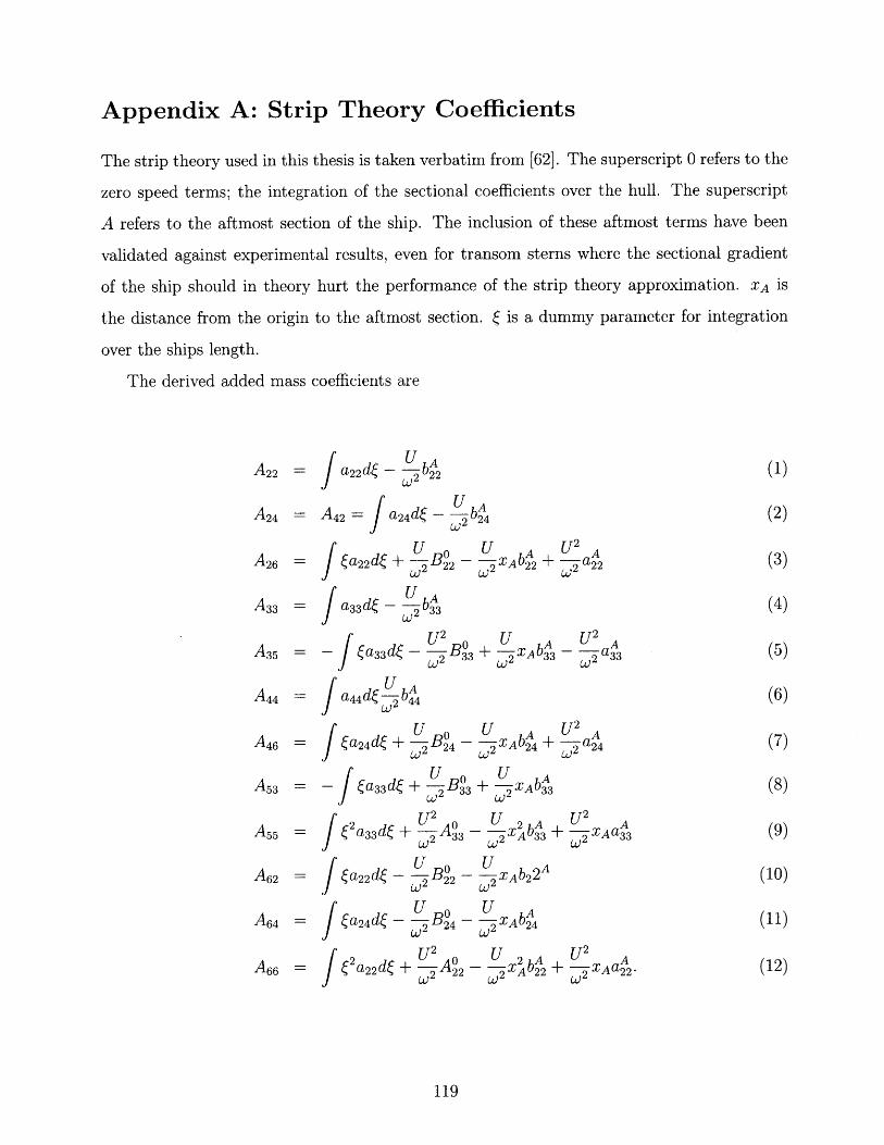
Appendix A: Strip Theory Coefficients

The strip theory used in this thesis is taken verbatim from [62]. The superscript 0 refers to the

zero speed terms; the integration of the sectional coefficients over the hull. The superscript

A refers to the aftmost section of the ship. The inclusion of these aftmost terms have been

validated against experimental results, even for transom sterns where the sectional gradient

of the ship should in theory hurt the performance of the strip theory approximation. XA is

the distance from the origin to the aftmost section. ( is a dummy parameter for integration

over the ships length.

The derived added mass coefficients are

A2 2 = a22 b (1)

A24 = A 42 = a24 d - bA (2)

A U U A U AA26 = Xa22b + B2 2 2b + 2a (3)

A33 = a3ad( - U (4)j 2 UU

A35 = - a33 ~ U2 Bs + 2 XAb A 2 aA (5)

fUA 4 4 = a44d( b^4 (6)

A4 6 + U Ba - U X A U2 A4 2 24 W2 b2 4 ± 2 (7)

A53 - J a3 3 d(+ B 3 + -XAb A (8)

A55 = f 32a33 + 3A2 3 + - U A 2 zaa (9)

A62 J (a 22d - 2 2 XAb 22 (10)/ U U

A 64 = Ja 24ck- 4BO -4 XAb2/ UU UA66 = U2a22+ 2 A 2 2 bA 2 . (12)

/6 fW222 A ~~~22 + L TXAa2.(2

119

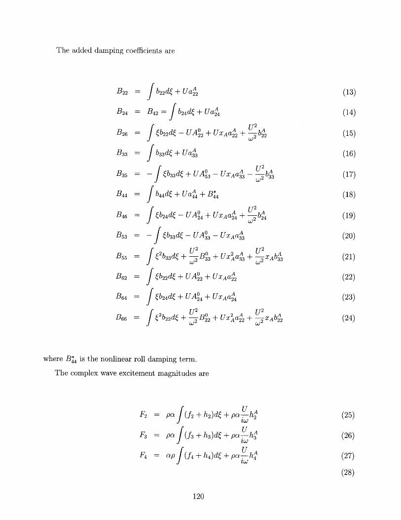
The added damping coefficients are

B 22 = b22 d+ UaA (13)

B 24 = B42 = b24 d +UaA (14)

B26 = Jb 22d - UA 2 + Uxa + b2 (15)

B33 = bs3 d + Ua A (16)

B335 - Jb 3 3d + UA 3 - UXAa - b (17)

B444 = Jb 4 4 dk+Ua4+B*4 (18)

B 46 = Jb 24d - UA04 + UXAaA + 2b (19)

B53 = - Jbs3dg - UA 3 - UXAa 3 (20)

B55 = f 2bs3d + u2 B3 + Ux2a3 + U2 ^A (21)L) 33 A2X '3

B62 J 1b 22dl + UA 2 + UXna22 (22)

B364 = Jb 24d 2 + UA 4 + UXna24 (23)

66 2b2d + U2 B + Ux2a2 ± 2 ^bA (24)

where B4 is the nonlinear roll damping term.

The complex wave excitement magnitudes are

F2 = pa (f 2 +h2 )d<+pa-iih A (25)

F3 = p C(f 3 +h 3 )d + pa-ihA (26)

F4 = ap (f 4 +h 4)d<+pa-LhA (27)

(28)

120

F5 = -pCa J (f +h3)+ - h

F6 = pa I(f 2+h2)+--h2

1d - pa-xXAhU A

d + pa-iWxxh2.

(29)

(30)

where p is density and a is wave amplitude.

Finally, the restoring forces are

C33

C35

C44

C55

(31)

(32)

(33)

(34)

where g is the gravitational constant, V is the displaced volume of the ship, and GM is the

metacentric height.

121

= pg bd

= Cs3 = -pg Jbd

= pgV(GM)

= pg J2bd

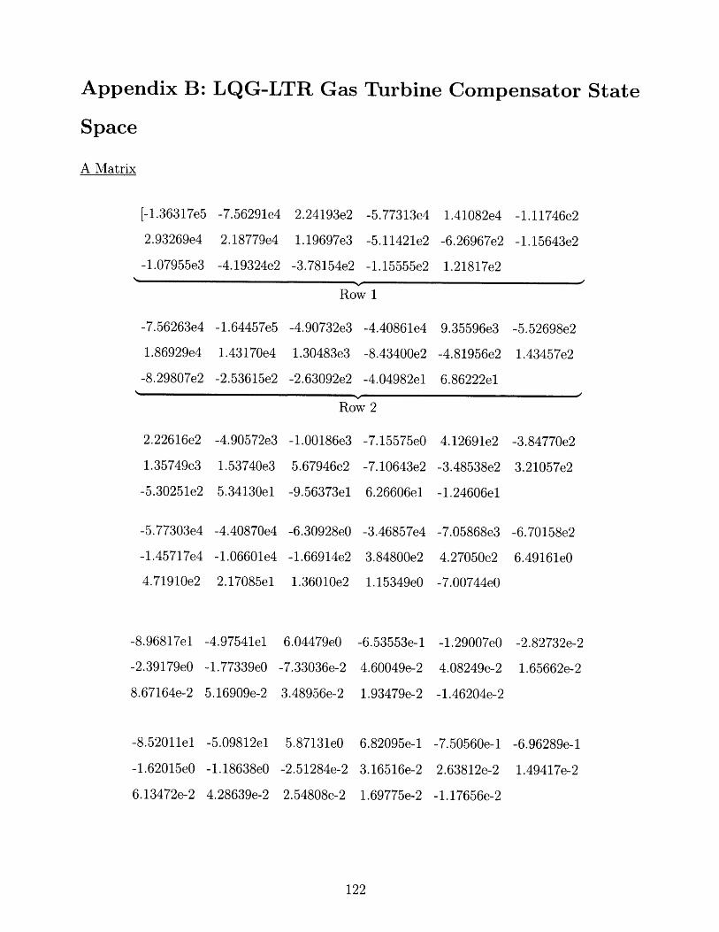
Appendix B: LQG-LTR Gas Turbine Compensator State

Space

A Matrix

[-1.36317e5

2.93269e4

-1.07955e3

-7.56291e4

2.18779e4

-4.19324e2

2.24193e2

1.19697e3

-3.78154e2

-5.77313e4

-5.11421e2

-1.15555e2

1.41082e4

-6.26967e2

1.21817e2

-1.11746e2

-1. 15643e2

Row I

-4.90732e3 -4.40861e4

1.30483e3 -8.43400e2

-2.63092e2 -4.04982el

Row 2

2.22616e2

1.35749e3

-5.30251e2

-5.77303e4

-1.45717e4

4.71910e2

-8.96817el

-2.39179e0

8.67164e-2

-8.52011el

-1.62015e0

6.13472e-2

-4.90572e3

1.53740e3

5.34130el

-4.40870e4

-1.06601e4

2.17085el

-4.97541el

-1.77339e0

5.16909e-2

-5.09812el

-1. 18638e0

4.28639e-2

-1.00186e3

5.67946e2

-9.56373el

-6.30928e0

-1.66914e2

1.36010e2

6.04479e0

-7.33036e-2

3.48956e-2

5.87131e0

-2.51284e-2

2.54808e-2

-7.15575e0

-7.10643e2

6.26606el

-3.46857e4

3.84800e2

1.15349e0

-6.53553e-1

4.60049e-2

1.93479e-2

6.82095e-1

3.16516e-2

1.69775e-2

4.12691e2

-3.48538e2

-1.24606el

-7.05868e3

4.27050e2

-7.00744e0

-1.29007e0

4.08249e-2

-1.46204e-2

-7.50560e-1

2.63812e-2

-1.17656e-2

-3.84770e2

3.21057e2

-6.70158e2

6.49161e0

-2.82732e-2

1.65662e-2

-6.96289e-1

1.49417e-2

122

-7.56263e4

1.86929e4

-8.29807e2

-1.64457e5

1.43170e4

-2.53615e2

9.35596e3

-4.81956e2

6.86222el

-5.52698e2

1.43457e2

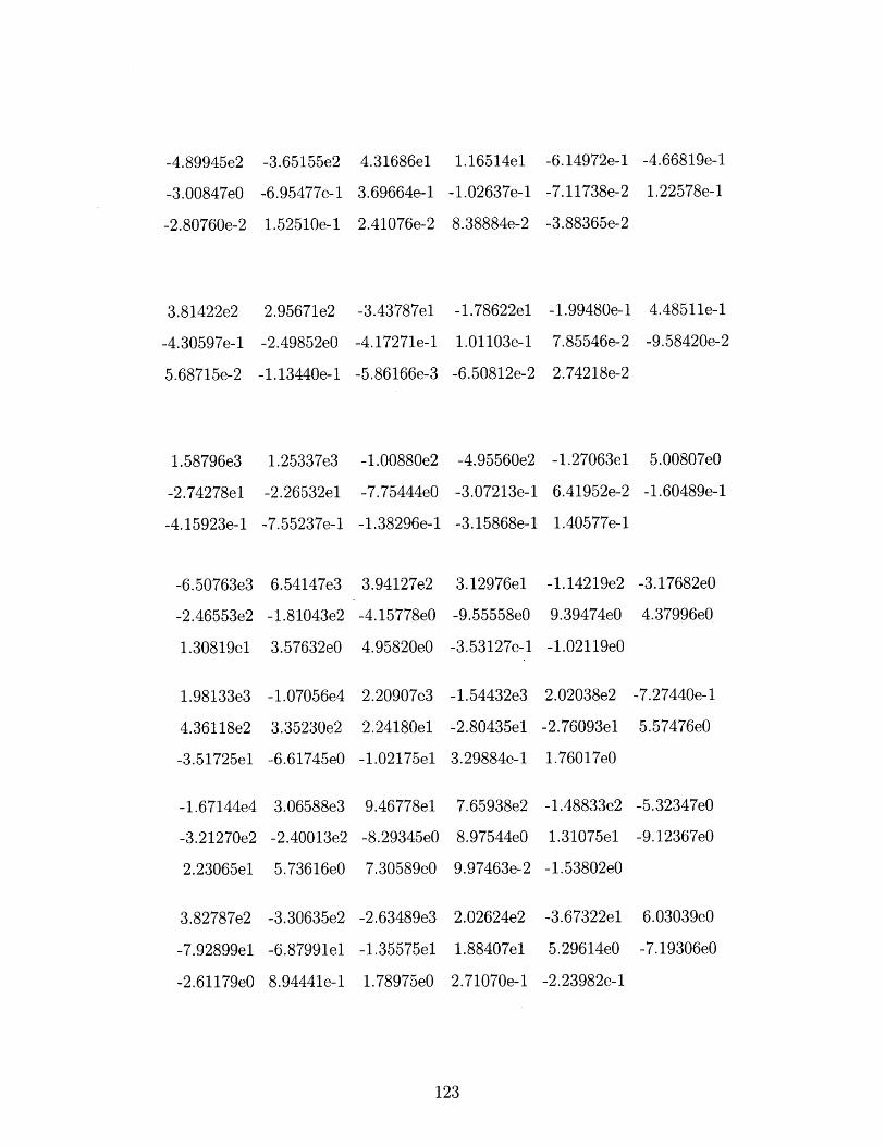
-4.89945e2

-3.00847e0

-2.80760e-2

3.81422e2

-4.30597e- 1

5.68715e-2

1.58796e3

-2.74278el

-4.15923e-1

-6.50763e3

-2.46553e2

1.30819el

1.98133e3

4.36118e2

-3.51725el

-1.67144e4

-3.21270e2

2.23065el

3.82787e2

-7.92899el

-2.61179e0

-3.65155e2

-6.95477e-1

1.52510e-1

2.95671e2

-2.49852e0

-1. 13440e-1

1.25337e3

-2.26532el

-7.55237e-1

6.54147e3

-1.81043e2

3.57632e0

-1.07056e4

3.35230e2

-6.61745e0

3.06588e3

-2.40013e2

5.73616e0

-3.30635e2

-6.87991el

8.94441e-1

4.31686el

3.69664e-1

2.41076e-2

-3.43787el

-4.17271e-1

-5.86166e-3

-1.00880e2

-7.75444e0

-1.38296e-1

3.94127e2

-4.15778e0

4.95820e0

2.20907e3

2.24180e1

-1.02175el

9.46778el

-8.29345e0

7.30589e0

-2.63489e3

-1.35575el

1.78975e0

1.16514el

-1.02637e-1

8.38884e-2

-1.78622el

1.01103e-1

-6.50812e-2

-4.95560e2

-3.07213e-1

-3.15868e-1

3.12976el

-9.55558e0

-3.53127e-1

-1.54432e3

-2.80435el

3.29884e-1

7.65938e2

8.97544e0

9.97463e-2

2.02624e2

1.88407el

2.71070e-1

-6.14972e-1

-7.11738e-2

-3.88365e-2

-1.99480e-1

7.85546e-2

2.74218e-2

-1.27063el

6.41952e-2

1.40577e-1

-1.14219e2

9.39474e0

-1.02119e0

2.02038e2

-2.76093el

1.76017e0

-1.48833e2

1.31075el

-1.53802e0

-3.67322el

5.29614e0

-2.23982e-1

-4.66819e-1

1.22578e-1

4.48511e-1

-9.58420e-2

5.00807e0

-1.60489e-1

-3.17682e0

4.37996e0

-7.27440e-1

5.57476e0

-5.32347e0

-9.12367e0

6.03039e0

-7.19306e0

123

-3.62200e3

1.66023el

-6.14798e0

-8.13921e3

1.22518e2

-9.16720e0

-1.97888e3

-1 .44480e2

6.65259e0

4.60768e2

3.51315el

-1.72108e0

-1.39242e3

1.67395el

-1.84894el

-9.83880e3

9.60949el

-6.10083e0

3.24868e3

-1. 13095e2

8.80035e-1

6.31139e2

2.92859el

1.52147e-2

2.00181e3

4.01861e0

3.61223e0

2.80868e3

9.42092e0

-2.03132el

-1.40270e3

-1.28464el

1.95008e0

8.72154e2

5.59118e0

-3.19137e-1

-1.90224e3

-1.11726el

-8.43531e-2

-5.95949e2

-8.89398e0

1.46755e-1

-2.84442e3

6.43206e0

-2.13870e1

1.05599e3

-4.01960e0

-8.48886e-1

7.69126e0

-3.43161e0

1.21722e-1

5.67584el

-5.52364e0

3.75213e-1

-6.69323el

4.12505e0

4.92849e-1

1.62752el

-1 .04473e0

-2.13009e1]

-2.04382e-1

4.26481e0

-3.27628e0

2.47021e0

7.08851e0

-1.63816e0

-3.66577e0

1.58754e0

B Matrix

[1.29674e-1

-1.20641e0

-8.96470e0

6.62556e-1

-3.87728e0

-3.21274e0

-2.55223el

1.89339el

-2.02993el

-1.09886e3

-1.40667e3

1.13568e-1

9.55107e-1

3.68070e0

-5.84756e0

-3.26135e0

-6.03087e0

-5.27942el

5.23846el

6.76094e2

8.22379e2

5.74499e2

1.11324e0

-2.72098e0

-3.49988e0

1.89355e-1

5.99098e0

6.23437e0

4.70611el

-3.87782el

-1.77869e2

-2.02415e3

1.99734e3

5.16370e-1

-8.99678e-1

8.56021e-1

1.34022e0

-6.00364e0

-4.06676e0

-3.33210e0

-1.08084e0

-6.88467el

-6.18874e2

1.09470e3

124

-2.05103e2

-7.46668e2

8.50472e2

-3.65534el

6.55729e2

-1.37986e2

-1.78074e3

7.32626e2

-3.18401e2

3.88125e2

-2.55542e2

-1.70413e2

-2.24253e2 5.77308e4

-1.19697e3 5.11415e2

3.78149e2 1.15555e2

RowI

4.90745e3 4.40867e4

-1.30484e3 8.43399e2

2.63099e2 4.04978el

RowI

1.00193e3

-5.67881e2

9.56291el

6.25884e0

1.66971e2

-1.36012e2

6.25884e0

7.10550e2

-6.26615el

3.46863e4

-3.84802e2

-1. 15349e0

125

-1.73200e2

1.77662e3

-1.09326e3

-5.91203e2

3.32767e2

-3.64031e2

-8.06422e2

-1.99026e2

4.16735el

3.07534e2

-3.62659e2

8.81838el]

C Matrix

[1.36316e5

-2.93267e4

1.07954e3

7.56272e4

-1.86933e4

8.29827e2

-2.24253e2

-1.35715e3

5.30206e2

5.77308e4

1.45723e4

-4.71913e2

7.56272e4

-2.18777e4

4.19320e2

1.64461e5

-1.43172e4

2.53620e2

4.90745e3

-1.53709e3

-5.34163el

4.40867e4

1.06606e4

-2.17078el

-1.41081e4

6.26959e2

-1.21816e2

-9.35613e3

4.81969e2

-6.86237el

-4.12533e2

3.48513e2

1.24614el

7.05893e3

-4.27054e2

7.00793e0]

1.11749e2

1.15642e2

5.52694e2

-1.43452e2

3.84740e2

-3.21021e2

6.70114e2

-6.49210e0

Bibliography

[1] ABKOWITZ, M. A. Stability and Motion Control of Ocean Vehicles. MIT Press, 1969.

[2] ALBERTOS, P., AND SALA, A. Multivariable Control Systems: An Engineering Ap-

proach, 1st ed. Springer, 2003.

[3] ANDRUS, M. Rtds notional e-ship model technical guide-version 2.1a. Tech. rep., FSU -

Center for Advanced Power Systems, July 2006.

[4] BASH, M., ET AL. A medium voltage dc testbed for ship power system research. In

IEEE Electric Ship Technologies Symposium (Baltimore MD, Apr. 2009).

[5] BECK, R., AND MAGEE, A. Time-domain analysis for predicting ship motions. In The

Dynamics of Marine Vehicles and Structures in Waves. Elsevier Science Ltd, 1991.

[6] BERNITSAS, M., RAY, D., AND KINLEY, P. Kt, kq and efficiency curves for the

wageningen b-series propellers. Tech. Rep. 237, The University of Michigan. Dept. of

Naval Architecture, May 1981.

[7] BISHOP, R., PRICE, W., AND TAM, P. Hydrodynamic coefficients of some heaving

cylinders of arbitrary shape. International Journal for Numerical Methods in Engineering

13 (1978), 17-33.

[8] CALIFANO, A., AND STEEN, S. Analysis of different propeller ventillation mechanisms

by means of rans simulations. In First International Symposium on Marine Propulsors

(Trondheim, Norway, June 2009).

126

[9] CHALFANT, J., CHRYSSOSTOMIDIS, C., AND ANGLE, M. Study of parallel ac and dc

electrical distribution in the all-electric ship. In Proceedings of the 2010 Grand Challanges

in Modeling and Simulation (Ottawa, Canada, Nov. 2010).

[10] CHEN, L., MIN, Y., XU, F., AND WANG, K.-P. A continuation-based method to

compute the relevant unstable equilibrium points for power system transient stability

analysis. IEEE Transactions on Power Systems 24, 1 (Feb. 2009), 165-172.

[11] CHOWDHURY, S., AND CROSSLY, P. Microgrids and Active Distribution Networks.

Institution of Engineering and Technology, July 2009.

[12] CLARKE, F. Stability analysis of sliding-mode feedback control. Control and Cybernetics

38, 4 (2009), 1169-1192.

[13] DEGROOT, M., AND SCHERVISH, M. Probability and Statistics, 3rd ed. Addison-Wesley,

Boston, MA, 2002.

[14] DENIS, M. S., AND PIERSON, W. On the motion of ships in confused seas. SNAME

Transl. 61 (1953).

[15] DOERRY, N., AND FIREMAN, H. Designing all electric ships. In Proceedings of the Ninth

International Marine Design Conference (Ann Arbor, MI, May 2006).

[16] DOUGAL, R. Design tools for electric ship systems. In Electric Ship Technologies Sym-

posium (July 2005), IEEE.

[17] ENGELBERG, S. Limitations of the describing function for limit cycle prediction. IEEE

Transactions of Automatic Control 47, 11 (2002), 1887-1890.

[18] Epps, B., CHALFANT, J., KIMBALL, R., TECHET, A., FLOOD, K., AND CHRYS-

SOSTOMIDIS, C. Openprop: An open-source parametric design and analysis tool for

propellers. Tech. rep., Massachusetts Institute of Technology, 2009.

[19] ERICSEN, T. Electric ship research and development consortium background, 2007.

http://esrdc.caps.fsu.edu/index.html.

127

[20] ERSELCAN, I. A frequency domain strip theory applied to the seakeeping of the zumwalt-

class destroyer. Master's thesis, Massachusetts Institute of Technology, May 2010.

[21] ESRDC, May 2010. The 2010 ESRDC Annual Team Meeting.

[22] FOSSEN, T. I. A nonlinear unified state-space model for ship maneuvering and control

in a seaway. Journal of Bifurication and Chaos (Sept. 2005).

[23] FOSSEN, T. I., AND FJELLSTAD, O.-E. Nonlinear modelling of marine vehicles in 6

degrees of freedom. Journal of Mathematical Modelling of Systems 1, 1 (1995).

[24] FRANK, W., AND SALVESEN, N. The frank close-fit ship motions computer program.

Tech. Rep. 3289, NSRDC, June 1970.

[25] FRIEDMAN, N.

2004.

U.S Destroyers. An Illustrated Design History. Naval Institute Press,

[26] G E MARINE. LM2500 Marine Gas Turbine, 2006.

[27] GELB, A. Multiple-Input describing functions and nonlinear systems. McGraw Hill Inc.,

1968.

[28] GREYTAK, M. High performance path following for marine vehicles using azimuthing

podded propulsion. Master's thesis, Massachusetts Institute of Technology, Feb. 2006.

[29] HOLMES, M. Introduction to Perturbation Methods.

1995.

Springer-Verlag New York, Inc.,

[30] HONG, Y. Prediction of Motions of SWATH Ships in Following Seas. David W Taylor

Naval Ship Research and Development Center, 1981.

[31] HOVER, F., AND TRIANTAFYLLOU, M. System design for uncertainty: Concepts, equa-

tions, and examples, 2009. Lecture Notes.

[32] IKEDA, Y., HIMENO, Y., AND TANAKA, N. Components of roll damping of ship at

forward speed. Journal of the Society of Naval Architecture Japan 143 (1978).

128

[33] JOHNSON, M., AND MORADI, M. PID Control: New Identification and Design Methods.

Springer, 2005.

[34] JONG, B. Computation of the hydrodynamic coefficients of oscillating cylinders. Tech.

Rep. 145, Netherlands Research Center TNO, 1973.

[35] JULIAN, A., AND CUZNER, R. Design, modeling and stability analysis of an integrated

shipboard dc power system. In Electric Ship Technologies Symposium (Baltimore MD,

Apr. 2009), IEEE, pp. 428-432.

[36] KAPPOS, E. Robust multivariable control for the f100 engine. Master's thesis, Mas-

sachusetts Institute of Technology, 1983.

[37] KERREBROCK, J. L. Aircraft Engines and Gas Turbines. The MIT Press, Apr. 1992.

[38] KERWIN, J. 13.04 lecture notes: Hydrofoils and propellers, 2001. Lecture Notes.

[39] KHAHIL, H. Nonlinear Systems, 3rd ed. Prentice Hall, 2002.

[40] KRAUSE, P. C. Analysis of Electric Machinery. Institue of Electrical and Electronics

Engineering, Jan. 1995.

[41] LEVEDAHL, W. Integrated electrical power supply system for propulsion and service

control. United State Patent Dept., Nov. 1997. 5684690.

[42] LEWIS, E. V. Volume iii motions in waves and controllability. In Principles of Naval

Architecture, 2nd ed. Society of Naval Architects and Marine Engineer, 1990.

[43] Lipo, T., AND KRAUSE, P. Stability analysis of a rectifier-inverter induction motor

drive. IEEE Transactions on Power Apparatus and Systems, 1 (Jan. 1969).

[44] Liu, J. Monte Carlo Strategies in Scientific Computing. Springer, 2004.

[45] Loop, B., SUDHOFF, S., ZAK, S., AND Zivi, E. Estimating regions of asymptotic

stability of power electronics systems using genetic algorithms. IEEE Transactions on

Control Systems Technology (2009).

129

[46] LORENZ, R. D., AND HAINES, L. P. Understanding Modern Power Conversion, 3rd ed.

University of Wisconsin, Jan. 2000.

[47] LOUKAKIS, T. A. Computer aided prediction of seakeeping performance in ship design.

Tech. Rep. MA-RD-900-71-8, Massachusetts Institute of Technologoy, Dec. 1970.

[48] MALESCI, C. Use of seakeeping simulation capabilities in the preliminary phase of the

design of multihull vessels. Master's thesis, Massachusetts Institute of Technology, June

2006.

[49] MARDEN, M., CHRYSSOSTOMIDIS, C., AND KARNIDAKAS, G. Mit model of the purdue

dc testbed. Tech. rep., Massachusetts Institute of Technology, 2009.

[50] THE MATHWORKS. Simulink User's Guide: Accelerating Modes, 2010. http: //www.

mathworks. com/ac c ess/helpdesk/help/t oolbox/s imulink/s imulink-product..page.

html.

[51] MENARD, P. Prediction of performance and maneuvering dynamics for marine vehicles

applied to ddg-1000. Master's thesis, Massachusetts Institute of Technology, May 2010.

[52] MOHAN, N., UNDELAND, T., AND ROBBINS, W. Power Electronics, Converters, Ap-

plications and Design. John Wiley and Sons Inc., 1995.

[53] MPT CONSULTANCY. Gas Turbine Electric Drive LNG Carrier, 2004. http: //www.

mptconsult.com/LNGCX/20GTG.htm.

[54] NEWMAN, J. Second-order slowly-varying forces on vessels in irregular waves. In In-

ternational Symposium Dynamics of Marine Vehicles and Structures in Waves (London

UK, Apr. 1974).

[55] NSWC. ASSET User's Manual, 1990.

[56] O.M. FALTINSEN, K.J. MINSAAS, N. L., AND SKJORDAL, S. Prediction of resistance

and propulsion of a ship in a seaway. In Proceedings of the Thirteenth Symposium on

Naval Hydrodynamics (Tokyo, 1980).

130

[57] PETERSON, H., AND KRAUSE, P. A direct- and quadrature-axis representation of par-

allel ac and de power system. IEEE Transactions on Power Apparatus and Systems 85,

3 (1966).

[58] PRATT AND WHITNEY. Product:Military:F100, 2010. http://www.pw.utc.com/

Products/Military/F100.

[59] PREMPRANEERACH, P., KIRTLEY, J., CHRYSSOSTOMIDIS, C., TRIANTAFYLLOU, M.,

AND KARNIDAKAS, G. Design of the all-electric ship: Focus on integrated power system

coupled to hydrodynamics. Tech. rep., Massachusetts Institute of Technology, 2008.

[60] RUBIS, C. Braking and reversing ship dynamics. Naval Engineering Journal 82, 1 (1970),

65-76.

[61] SALVESEN, N. Second-order steady-state forces and moment on surface ships in oblique

regular waves. In The Dynamics of Marine Vehicles and Structures in Waves. Elsevier

Science Ltd, 1975, pp. 212-226.

[62] SALVESEN, N., TUCK, E., AND FALTINSEN, 0. Ship motions and sea loads. SNAME

Transl. 78 (1970).

[63] SCHANK, ET AL. Acquisition and Competition Strategy for the DD(X). The U.S. Navy's

21st Century Destroyer. The RAND Corporation, 2006.

[64] SCHMITT, K., AND TRIANTAFYLLOU, M. Modeling and simulation of the all electric

ship in random seas including supplemental material. Tech. rep., Massachusetts Institute

of Technology, 2010.

[65] SMOGELI, 0. N. Control of Marine Propellers. From Normal to Extreme Conditions.

PhD thesis, Norwegian University of Science and Technology, Sept. 2006.

[66] SOULTATISI, C. Systems modeling for electric ship design. Master's thesis, Massachusetts

Institute of Technology, June 2004.

[67] STETTLER, J. W. Steady and Unsteady Dynamics of an Azimuthing Podded Propulsor

Related to Vehicle Maneuvering. PhD thesis, Massachusetts Institute of Technology, May

2004.

131

[68] SUDHOFF, S., ET AL. Admittance space stability analysis of power electronic systems.

IEEE Transactions on Aerospace and Electronic Systems 36, 3 (July 2000).

[69] TRIANTAFYLLOU, M. 2.22 design principles for ocean vehicles, 2010. Lecture Notes.

[70] TRIANTAFYLLOU, M., AND HOVER, F. Maneuvering and control of marine vehicles,

2002. Lecture Notes.

[71] VUGTS, J. The hydrodynamic coefficients for swaying, heaving and rolling cylinders in

a free surface. Tech. Rep. 112S, Netherlands Research Center TNO, 1968.

[72] WELCH, P. The use of fast fourier transform for the estimation of power spectra: A

method based on time averaging over short, modified periodograms. IEEE Transactions

on Audio Electroacoustics AU-15 (1967), 70-73.

[73] WELSH, M., Jul 2010. Interview Regarding the Challenges and Advantages of an All

Electric Ship.

132

Modeling and Simulation of an All Electric Ship

Documents

Transcript of Modeling and Simulation of an All Electric Ship