Modeling and operation of hybrid ferry with gas engine ...
98
Modeling and operation of hybrid ferry with gas engine, synchronous machine and battery Martin Skaar Vadset Master of Energy Use and Energy Planning Supervisor: Trond Toftevaag, IEL Co-supervisor: Bernt Ove Sunde, Vard Electro Department of Electric Power Engineering Submission date: June 2018 Norwegian University of Science and Technology
Transcript of Modeling and operation of hybrid ferry with gas engine ...

Modeling and operation of hybrid ferrywith gas engine, synchronous machineand battery
Martin Skaar Vadset
Master of Energy Use and Energy Planning
Supervisor: Trond Toftevaag, IELCo-supervisor: Bernt Ove Sunde, Vard Electro
Department of Electric Power Engineering
Submission date: June 2018
Norwegian University of Science and Technology


i
Preface
This project report represents my master’s thesis and complete my degree from Norwegian Uni-
versity of Science and Technology (NTNU) in Trondheim. The thesis builds on my specialisation
project “Optimal operation of hybrid ferry with gas engine, synchronous machine and battery”,
which was developed in the autumn of 2017. For the master’s thesis, further investigation into
power solutions for the LNG ferry designed by Vard Electro is conducted.
An essential component of this thesis was to develop a simulation model of the electrical system
in Simscape Power Systems. The goal of the simulation was to model fuel consumption from a
given load profile and investigate the performance of the system. Another part includes rules
for classification of ships and the limitations of the classifications on the flexibility of the power
system on board a ferry.
I would like to thank my supervisor Trond Toftevaag for his crucial help and keeping his door
open to me throughout the project. Also, thanks go to Vard Electro, Bernt Ove Sunde and Ulf
Ødegaard for offering me the opportunity to work with this interesting problem and their help
with questions and information related to the task.
Trondheim, 2018-06-05
Martin Skaar Vadset

ii
Abstract
In this master’s thesis, a direct current (DC) hybrid energy system for a liquified natural gas
(LNG) ferry is developed and studied. The system is constructed in Matlab and Simulink and
consists of two generator sets with gas engines and synchronous generators, six-pulse diode
rectifiers, battery storage, bi-directional DC/DC converter and a load. A control structure for
the gas engine, excitation system of the generators and battery converter is developed. The gas
engine is modelled with the GAST model and a speed governor, while the excitation system is
modelled with the AC1A excitation model and droop control with respect to the DC link voltage.
Two control methods are developed for the control of the converter, droop and peak shaving.
The performance of the controllers and system is tested for generator sets with droop control,
generator sets and battery with droop control and peak shaving with generator sets and battery.
The specific energy consumption (SEC) of the gas engines is then calculated for fixed and vari-
able speed during stationary operation with respect to the engine speed and engine load. The
SEC values are compared for the cases and with respect to variable and fixed speed.
Variable speed resulted in lower SEC for all cases presented, and the highest difference was
for the case with the peak shaving method. For the droop control configuration between the
generator sets and the battery, the SoC limits of 80-65 % was violated with a δB at equal 0.05.
Then, the options for the system were to increase δB at and reduce the contribution from the
battery or install a larger battery that is able to contribute the load power without violating the
SoC limits. With the peak shaving method, stored power was available in the battery since the
SoC was in the range of 80-76 %. With the discharge and charging power (±1800 kW) delivered
from the battery, a smaller battery with a capacity of 720 kWh could obtain the same operation.
An opportunity to reduce the SEC of the operation is to develop a control system for connecting
and disconnecting generators sets, which makes the generator sets operate at a more optimal
loading rate.

iii
Sammendrag
I denne masteroppgåva har eit hybrid likestraums system (DC) for ein flytande naturgass (LNG)
ferje blitt utvikla og studert. Systemet består av to generatorsett med gassmotorar og synkro-
ngeneratorar, seks-pulsa diode likerettarar, batteri lagringssystem, tovegs DC/DC konverter og
ein last. Sjølve simuleringsmodellen er konstruert i Matlab og Simulink, der kontrollsystemet for
gassmotorane, eksiteringssystemet for generatorane og batterikonverteren er utvikla. Gassmo-
torane er modellert med GAST modellen og ein hastigheits regulator, medan eksiteringssys-
temet er modellert med AC1A eksiterings modell og ein statikk kontroller med omsyn på spen-
ninga på DC samleskinna. Kontrollaren for batterikonverteren er regulert ved to metodar, last-
fordeling ved ein statikkfaktor og kutting av last toppane. Kontrollaren og systemet si yting
er testa ved ulike operasjonsstrategiar, der generatorsetta opererar åleine og saman med bat-
teriet. Strategiane er lastfordeling mellom generatorsetta ved statikk kontroll, lastfordeling mel-
lom generatorsett og batteri ved statikk kontroll og at batteriet tar last toppane, medan gen-
eratorsetta fordelar den resterande lasta mellom seg. Det spesifikke energi forbruket (SEC) av
gassmotoren er så kalkulert for bestemt og variabel hastigheit med omsyn til motor hastigheit og
last. Det ulike SEC forbruket er så samanlikna for operasjonsstrategiane med omsyn til bestemt
og variabel hastigheit.
Variabel hastigheit resulterte i lågare SEC for alle metodane som vart presentert, og den største
forskjellen var for metoden med kutting av last toppane. Batteriets ladestatus (SoC) grenser
vart ikkje oppretthalde med statikk kontroller metoden, når δB at var 0.05. For at grensene ikkje
skal overstigast kan ein auke statikkfaktoren δB at og dermed redusere bidraget frå batteriet. Ei
anna moglegheit er å installere eit batteri med høgare kapasitet slik at batteriet kan bidra med
effekt utan at SoC grensene blir overstege. Når kutting av last topp metoden blei nytta var der
tilgjengeleg effekt i batteriet ettersom SoC opererte i område 80-76 %. Ei moglegheit for sys-
temet når batteriet blir ladda og utloddast med 1800 kW var å installere eit mindre batteri med
ein kapasitet på 720 kWh. Dette batteriet kan utføre den same operasjonen, men er eit mindre
og billigare alternativ. Ei anna moglegheit for å redusere SEC er å utvikle eit kontrollsystem for
innkopling og utkopling av generatorsett, dette kan gjer slik at generatorane arbeidar på eit meir
optimalt lastpunkt med tanke på forbruk.

Contents
Preface . . . . . . . . . . . . . . . . . . . . . . . . . . . . . . . . . . . . . . . . . . . . . . . . i
Abstract . . . . . . . . . . . . . . . . . . . . . . . . . . . . . . . . . . . . . . . . . . . . . . . . ii
Sammendrag . . . . . . . . . . . . . . . . . . . . . . . . . . . . . . . . . . . . . . . . . . . . iii
Acronyms . . . . . . . . . . . . . . . . . . . . . . . . . . . . . . . . . . . . . . . . . . . . . . vii
1 Introduction 1
1.1 Problem description . . . . . . . . . . . . . . . . . . . . . . . . . . . . . . . . . . . . . 2
1.2 Limitations . . . . . . . . . . . . . . . . . . . . . . . . . . . . . . . . . . . . . . . . . . . 2
1.3 Software . . . . . . . . . . . . . . . . . . . . . . . . . . . . . . . . . . . . . . . . . . . . 3
1.4 Structure of the Report . . . . . . . . . . . . . . . . . . . . . . . . . . . . . . . . . . . . 3
2 System description 4
2.1 The vessel . . . . . . . . . . . . . . . . . . . . . . . . . . . . . . . . . . . . . . . . . . . 4
2.2 System description . . . . . . . . . . . . . . . . . . . . . . . . . . . . . . . . . . . . . . 4
3 Background 7
3.1 LVDC distribution in ship applications . . . . . . . . . . . . . . . . . . . . . . . . . . 7
3.2 Specific energy consumption . . . . . . . . . . . . . . . . . . . . . . . . . . . . . . . . 8
3.3 Batteries in LVDC distribution . . . . . . . . . . . . . . . . . . . . . . . . . . . . . . . 9
3.3.1 C-rate . . . . . . . . . . . . . . . . . . . . . . . . . . . . . . . . . . . . . . . . . . 12
3.4 Bi-directional DC/DC converter . . . . . . . . . . . . . . . . . . . . . . . . . . . . . . 12
3.5 Non-regenerative front-end rectifier (NFE) . . . . . . . . . . . . . . . . . . . . . . . . 14
4 Rules for classification of ships 16
4.1 Chapter 8 Electrical installations (Part 4) . . . . . . . . . . . . . . . . . . . . . . . . . 16
iv

CONTENTS v
4.2 Class notation Battery . . . . . . . . . . . . . . . . . . . . . . . . . . . . . . . . . . . . 17
5 Modelling of the system 18
5.1 Synchronous generator . . . . . . . . . . . . . . . . . . . . . . . . . . . . . . . . . . . 19
5.1.1 Regulator and excitation system . . . . . . . . . . . . . . . . . . . . . . . . . . 19
5.1.2 The synchronous generator-rectifier . . . . . . . . . . . . . . . . . . . . . . . . 21
5.2 Gas engine . . . . . . . . . . . . . . . . . . . . . . . . . . . . . . . . . . . . . . . . . . . 22
5.2.1 Gas turbine model (GAST) . . . . . . . . . . . . . . . . . . . . . . . . . . . . . 23
5.2.2 Speed governor . . . . . . . . . . . . . . . . . . . . . . . . . . . . . . . . . . . . 24
5.2.3 Variable speed controller . . . . . . . . . . . . . . . . . . . . . . . . . . . . . . 25
5.2.4 Calculation of SEC . . . . . . . . . . . . . . . . . . . . . . . . . . . . . . . . . . 26
5.3 Energy storage system . . . . . . . . . . . . . . . . . . . . . . . . . . . . . . . . . . . . 26
5.3.1 Modeling of the Bi-directional DC/DC converter . . . . . . . . . . . . . . . . 26
5.3.2 Converter parameters . . . . . . . . . . . . . . . . . . . . . . . . . . . . . . . . 28
5.3.3 Control system for the bi-directional converter . . . . . . . . . . . . . . . . . 29
5.3.4 Droop control . . . . . . . . . . . . . . . . . . . . . . . . . . . . . . . . . . . . . 33
5.3.5 Peak shaving control . . . . . . . . . . . . . . . . . . . . . . . . . . . . . . . . . 35
5.4 Limitations and evaluation of Chapter 5 . . . . . . . . . . . . . . . . . . . . . . . . . 37
6 Testing of the model 38
6.1 One generator set . . . . . . . . . . . . . . . . . . . . . . . . . . . . . . . . . . . . . . . 38
6.2 Two generator sets . . . . . . . . . . . . . . . . . . . . . . . . . . . . . . . . . . . . . . 40
6.3 Two generator sets and battery . . . . . . . . . . . . . . . . . . . . . . . . . . . . . . . 43
6.3.1 Load sharing . . . . . . . . . . . . . . . . . . . . . . . . . . . . . . . . . . . . . . 43
6.3.2 Peak shaving . . . . . . . . . . . . . . . . . . . . . . . . . . . . . . . . . . . . . . 45
6.4 Evaluation of Chapter 6 . . . . . . . . . . . . . . . . . . . . . . . . . . . . . . . . . . . 49
7 Simulations and results 50
7.1 Case 1: Droop control with generator sets . . . . . . . . . . . . . . . . . . . . . . . . . 51
7.2 Case 2: Droop control with generator sets and battery . . . . . . . . . . . . . . . . . 53
7.3 Case 3: Peak shaving with generator sets and battery . . . . . . . . . . . . . . . . . . 55
7.4 Case 4: Variable speed operation during peak shaving . . . . . . . . . . . . . . . . . 58

CONTENTS vi
7.5 Specific energy consumption of the cases . . . . . . . . . . . . . . . . . . . . . . . . . 60
7.6 Evaluation of Chapter 7 . . . . . . . . . . . . . . . . . . . . . . . . . . . . . . . . . . . 64
8 Conclusion 66
8.1 Further work . . . . . . . . . . . . . . . . . . . . . . . . . . . . . . . . . . . . . . . . . . 68
A Appendix A 69
A.1 Calculations of converter parameters . . . . . . . . . . . . . . . . . . . . . . . . . . . 69
A.2 Small signal average model of the converter . . . . . . . . . . . . . . . . . . . . . . . 70
A.3 Development of the cascade converter controller . . . . . . . . . . . . . . . . . . . . 71
A.3.1 Current controller . . . . . . . . . . . . . . . . . . . . . . . . . . . . . . . . . . 71
A.3.2 Voltage controller . . . . . . . . . . . . . . . . . . . . . . . . . . . . . . . . . . . 73
A.4 Calculations of fuel costs . . . . . . . . . . . . . . . . . . . . . . . . . . . . . . . . . . . 74
B Appendix B 76
B.1 The Simulink model . . . . . . . . . . . . . . . . . . . . . . . . . . . . . . . . . . . . . 76
B.2 Matlab script for calculation of SEC . . . . . . . . . . . . . . . . . . . . . . . . . . . . 77
B.3 Actual load scenario . . . . . . . . . . . . . . . . . . . . . . . . . . . . . . . . . . . . . 78
C Appendix C 79
C.1 Testing of the model . . . . . . . . . . . . . . . . . . . . . . . . . . . . . . . . . . . . . 79
D Appendix E 81
D.1 Synchronous generator parameters . . . . . . . . . . . . . . . . . . . . . . . . . . . . 81
D.2 Parameter Setting of excitation model AC1A . . . . . . . . . . . . . . . . . . . . . . . 82
D.3 Parameters setting of GAST and speed governor . . . . . . . . . . . . . . . . . . . . . 82
Bibliography 83

Acronyms
LVDC Low Voltage Direct Current
DC Direct Current
AC Alternating Current
SEC Specific Energy Consumption
LNG Liquified Natural Gas
DoD Depth-of-Cischarge
SoC State-of-Charge
SED Specific Energy Density
VED Volumetric Energy Density
NFE Non-Regenerative Front-End Rectifier
PID Proportional–Integral–Derivative
MCR Maximum continuous rating of engine
NOK Norwegian Krone
IMO International Maritime Organization
IEEE Institute of Electrical and Electronics Engineers
IGBT Insulated Gate Bipolar Transistor
vii

CONTENTS viii
PWM Pulse With Modulation
EMS Energy Management System
1 | Introduction
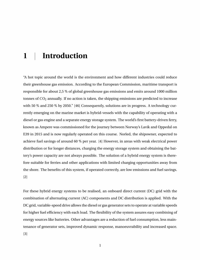
“A hot topic around the world is the environment and how different industries could reduce
their greenhouse gas emission. According to the European Commission, maritime transport is
responsible for about 2,5 % of global greenhouse gas emissions and emits around 1000 million
tonnes of CO2 annually. If no action is taken, the shipping emissions are predicted to increase
with 50 % and 250 % by 2050.” [46] Consequently, solutions are in progress. A technology cur-
rently emerging on the marine market is hybrid-vessels with the capability of operating with a
diesel or gas engine and a separate energy storage system. The world’s first battery-driven ferry,
known as Ampere was commissioned for the journey between Norway’s Lavik and Oppedal on
E39 in 2015 and is now regularly operated on this course. Norled, the shipowner, expected to
achieve fuel savings of around 60 % per year. [4] However, in areas with weak electrical power
distribution or for longer distances, charging the energy storage system and obtaining the bat-
tery’s power capacity are not always possible. The solution of a hybrid energy system is there-
fore suitable for ferries and other applications with limited charging opportunities away from
the shore. The benefits of this system, if operated correctly, are low emissions and fuel savings.
[2]
For these hybrid energy systems to be realised, an onboard direct current (DC) grid with the
combination of alternating current (AC) components and DC distribution is applied. With the
DC grid, variable-speed drive allows the diesel or gas generator sets to operate at variable speeds
for higher fuel efficiency with each load. The flexibility of the system assures easy combining of
energy sources like batteries. Other advantages are a reduction of fuel consumption, less main-
tenance of generator sets, improved dynamic response, manoeuvrability and increased space.
[3]
1
CHAPTER 1. INTRODUCTION 2
1.1 Problem description
This master’s thesis considers a hybrid energy system for a liquified natural gas (LNG) ferry de-
signed by Vard Electro. The topics addressed and the principles considered herein are as follows:
• The construction of a simulation model of the DC-grid hybrid power system consisting of
two generator sets with gas engines and synchronous generators, battery storage system
and a constant load.
• The development and testing of a control structure to control the speed of the gas engine,
the excitation system of the generators and the battery converter.
• The operation of the developed power system through a load profile with different opera-
tion profiles to address performance and fuel consumption
• A brief study of the classification of limitations and requirements for the power system
onboard ships.
1.2 Limitations
The modelled system is limited to two generator sets that comprise gas engines and synchronous
generators, one lithium-ion battery and one load. The parameters for the control systems do
not correspond to a real system. The goal of the simulations was to acquire a stable system with
realistic parameters that operates within acceptable performance criteria. To obtain a model
system which corresponds to a real system, parameters could be tuned to change the response.
With the discrete solver option in Simulink, there is a risk of deviations in the transients, such as
the, size of the over-voltage.

CHAPTER 1. INTRODUCTION 3
1.3 Software
The software programs used for this thesis are Matlab and Simulink. Matlab is a programming
language that expresses matrix and array mathematics directly in order to implement an it-
erative analysis and design processes. [18] For the simulations in Simulink, Simscape Power
Systems was used as it provides component libraries and analytical tools for the modeling and
simulation of electrical power systems. [20]
1.4 Structure of the Report
The rest of the report is structured as follows. Chapter 2 introduces and describes the vessel
and system. In Chapter 3, background information and theoretical approaches are presented.
Chapter 4 explains some rules of the classification of ships. Chapter 5 presents the approach
behind the modelling of the system, while Chapter 6 descries tests of the model. In Chapter
7, the simulation and results of the load profile are presented before the conclusion is given in
Chapter 8.

2 | System description
2.1 The vessel
The vessel under consideration is a LNG ferry, in which gas and an electrical hybrid propulsion
system with a battery are installed. This design makes the vessel suited to accommodate likely
future requirements like energy efficiency and low-emission technology. The shipbuilding com-
pany Vard has a contract to deliver two ferries at a total cost of 600 million NOK and these ships
should be delivered by Vard Breivik in 2018. This type of vessel is 130 meters long and 20.7 me-
ters wide, with a total capacity of 550 passengers, and it will operate at a speed of approximately
18 knots. On the main deck, there is room for 180 passenger cars. [22] (Citation from the Project
Rapport)
2.2 System description
The electrical power system of the vessel is shown in Figure 2.1. The system contains three LNG
generator sets with a rated power of 2589 kVA and a nominal voltage of 705 V. The generator sets
supply power to two propulsion engines and two passive loads together with a battery energy
storage system, wich has been rated at 1017 kWh. The battery charging and discharging limits
are 2542 kW (2,5C). Generator sets and loads are connected to a DC busbar through rectifiers
and inverters, while the battery is connected through a bi-directional DC/DC converter. The
voltage level on the DC-bus is 975 V. The original system constructed by Vard Electro has two
emergency diesel generators, and two main busses separated by galvanic isolation for safety
measures. The single-line diagram of the power system is presented in Figure 2.1. For the simu-
lations in Simulink, the power system has been reduced to two generator sets, battery and one
4

CHAPTER 2. SYSTEM DESCRIPTION 5
power load.
Figure 2.1: Single-line diagram of the power system for this study
With a variable-speed system, the prime movers can operate with a variable speed such that the
combustion is optimal based on the loading of the system. The operation of the generators is
determined from the speed of the prime movers, which gives an electrical frequency that varies
according to the speed of the prime movers. The generators used for this thesis have a frequency
range of 35-50 Hz. The rectifiers are non-regenerative front-end rectifiers, as a bi-directional
power flow is not necessary. [19] The battery, on the other hand, needs a bi-directional power
flow to discharge and charge. A bi-directional converter is therefore installed between the bat-
tery and the DC link to boost the voltage and control the power flow from the battery. The power
flow in the system is controlled by the battery management system, power management system
and the overall energy management system. For this thesis, only the controllers for the genera-
tor sets and the battery were investigated. The manner in which the battery affects the load flow
of the system is decided by the controller for the system. The operation modes (strategies) for
the battery investigated for this thesis are peak shaving and load sharing. During peak shaving,
the generators delivers average load power, while the energy storage system compensates for

CHAPTER 2. SYSTEM DESCRIPTION 6
variations in the load. When load sharing is selected, the load is distributed among the gener-
ators and the energy storage. The amount of power shared is decided by the controllers for the
battery and the generator sets. [49] The goals of a network system like this one are to obtain
optimal power generation, fuel savings and lower emissions from the battery and the variable
speed generators.

3 | Background
In this chapter, basic theories regarding key components of the project are presented.
3.1 LVDC distribution in ship applications
Ship applications with low voltage direct current (LVDC) distributions have been recently emerg-
ing on the market, with benefits like space utilisation, weight and fuel consumption. [42] Adding
additional components like an energy storage system to the network is simpler with DC dis-
tribution, as they can be connected directly to the network or through bi-directional DC/DC
converters. [50] With the DC distribution, generator sets can operate at variable speeds, which
offers a wider fuel-efficiency loading area than generators with fixed speeds. The prime movers
can adjust the speed depending on the load and power consumed with the help of an efficiency
optimal controller. However, the change in speed generates a slower response in power produc-
tion compared to the fixed speed generators. To compensate for the slow response, an energy
storage system could be added to the network to provide the remaining power required to keep
the DC bus voltage to a specific level. [53] The connected energy storage system leads to lower
emissions and less fuel consumption.[50]
In AC distribution, load sharing is controlled through speed regulation from the prime movers
and, based on the frequency droop, while the excitation system of synchronous generators con-
trols the voltage. In a DC power system, the only variable that the generators share is the DC
voltage, and the generators frequencies are independent within the system. The voltage regula-
tion and control of power sharing of the DC power system should therefore be controlled by the
excitation system of the synchronous generators. [23]
7

CHAPTER 3. BACKGROUND 8
3.2 Specific energy consumption
Improving the gas engine fuel efficiency is a means of reducing the operational costs of the sys-
tem. For the gas engines, the specific energy consumption (SEC) is used to investigate the energy
consumption. The SEC is defined as kilo-joules consumed per kilowatt hours produced. [33]
The gas engines have an optimal loading rate, such that the engine operates with the lowest fuel
consumption. The load point of the engine is usually not optimised during a voyage, as seen in
Figure 3.1. Connecting an energy storage system to the network could prevent the engine from
operating away from the optimal loading rate, which would result in lower fuel consumption
from the engines. [31]
Figure 3.1: Energy distribution for one month. The blue line indicates the optimal operationpoint. Source: [31]
The gas engines also have an optimal speed point for different loading conditions. For the DC
distribution, the variable speed of the generators can be optimised from the loading to reduce
the SEC of the engines accordingly. The load limit curve for a C26:33L gas engine from Rolls-
Royce is presented in Figure 3.2. The green line indicates the SEC for fixed speed, while the
curved line represents the optimal speed level for each load at variable speeds. By adjusting the
speed together with the load, a lower SEC could be accomplished. During fixed speed uses, the
SEC is highest for lower loads. The bold solid curve indicates the load limits of the engine re-
garding speed [rpm] and cylinder output [kW]. [57]

CHAPTER 3. BACKGROUND 9
Figure 3.2: Load limit curve for C26:33L gas engine. Source: [51]
3.3 Batteries in LVDC distribution
One of the most frequently used energy storage systems for hybrid power systems is batter-
ies, and it is an expensive part of the power system. The operating voltage from the battery
is achieved by connecting cells in series, and the total voltage potential from the cells creates
the terminal voltage. By adding cells in parallel, the capacity is increased by combining the to-
tal ampere-hour from each cell. [6] The nominal voltage from each cell is decided by the cell
chemistry and varies for each different configuration. The cell chemistry is described as the
electromechanical characteristics of the active chemicals used. When comparing the differ-
ent battery configurations from Figure 3.3, lithium-ion has a higher cell voltage and achieves a
higher terminal voltage with fewer cells.

CHAPTER 3. BACKGROUND 10
Figure 3.3: Discharge characteristics for different battery configurations. Source: [7]
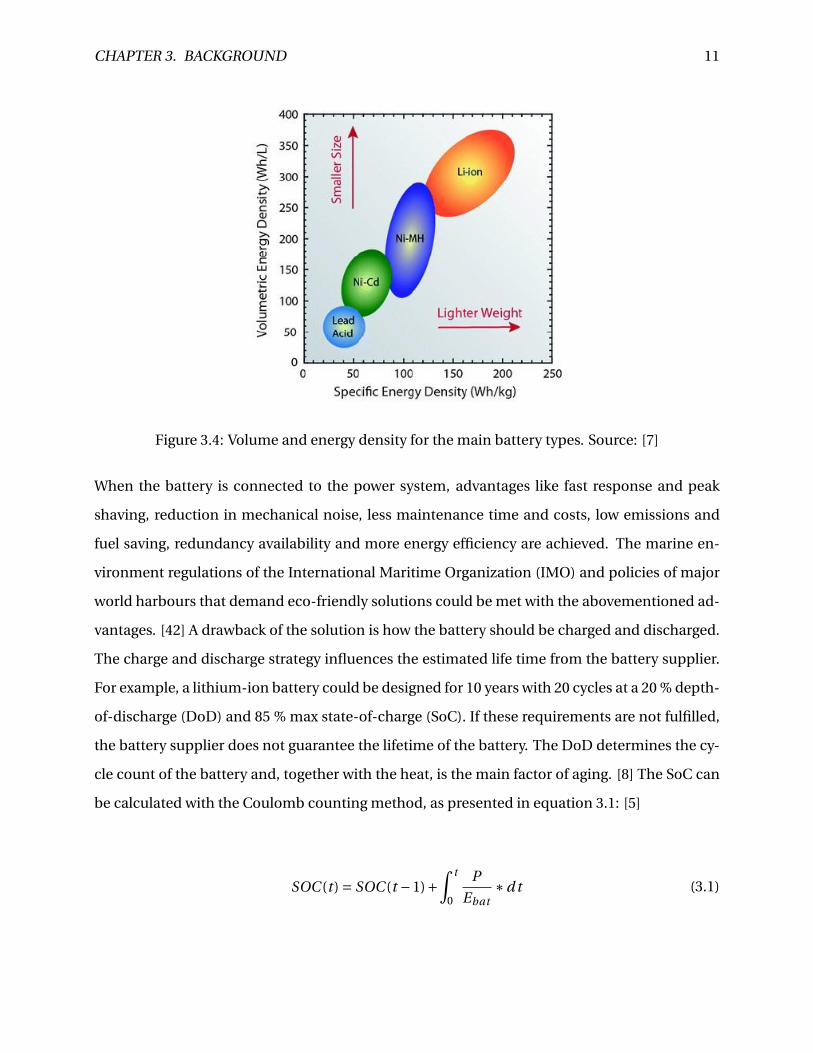
Another criterion for the battery is specific energy density (SED) [Wh/kg] and volumetric energy
density (VED) [Wh/l]. The VED is important for saving space a board the ship, while high energy
density could lead to instability in the electrochemistry of the battery. Batteries with high en-
ergy density must therefore be handled carefully, and the importance of a battery management
system is thus higher. As can be seen in Figure 3.4, lithium-ion batteries are beneficial in terms
of size and weight compared to the other battery technologies. [7]
CHAPTER 3. BACKGROUND 11
Figure 3.4: Volume and energy density for the main battery types. Source: [7]
When the battery is connected to the power system, advantages like fast response and peak
shaving, reduction in mechanical noise, less maintenance time and costs, low emissions and
fuel saving, redundancy availability and more energy efficiency are achieved. The marine en-
vironment regulations of the International Maritime Organization (IMO) and policies of major
world harbours that demand eco-friendly solutions could be met with the abovementioned ad-
vantages. [42] A drawback of the solution is how the battery should be charged and discharged.
The charge and discharge strategy influences the estimated life time from the battery supplier.
For example, a lithium-ion battery could be designed for 10 years with 20 cycles at a 20 % depth-
of-discharge (DoD) and 85 % max state-of-charge (SoC). If these requirements are not fulfilled,
the battery supplier does not guarantee the lifetime of the battery. The DoD determines the cy-
cle count of the battery and, together with the heat, is the main factor of aging. [8] The SoC can
be calculated with the Coulomb counting method, as presented in equation 3.1: [5]
SOC (t ) = SOC (t −1)+∫ t
0
P
Ebat∗d t (3.1)

CHAPTER 3. BACKGROUND 12
In the equation, SOC (t ) is the battery SoC at time t [%], SOC (t −1) is the battery’s initial SoC
in [%], t is the time [h], P is the charge/discharge power [kW] and Ebat is the battery capacity
[kWh]. [46]
3.3.1 C-rate
To express the discharge current in order to normalise it to the battery capacity, the C-rate is
often used. The battery capacity is usually referred as 1C, which indicates that the discharge
current will discharge the battery in one hour. [10] Batteries with a rated capacity of 1000 Ah
should provide 1000 A for one hour, as seen in Figure 3.5. In the figure, SoC [%] is the y-axis,
while the time [h] is the x-axis. The same battery should provide 2000 Ah for 30 minutes if the
rating is 2C. [8]
Figure 3.5: The SoC for different C-ratings constructed in Microsoft Excel (Simple model)
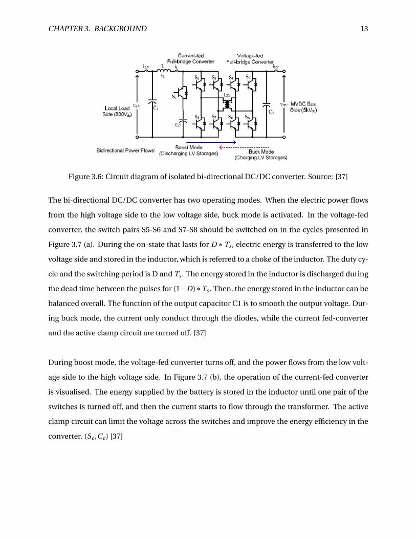
3.4 Bi-directional DC/DC converter
For stationary storage devices such as batteries, a bi-directional DC-DC interface is necessary
to control the charging and discharging processes. In the power system, the converter operates
between the battery system voltage and the voltage on the DC link. During charging, the con-
troller is in buck mode, while boost mode means the battery is discharging. A classical design of
a bi-directional DC/DC converter is presented in Figure 3.6.
CHAPTER 3. BACKGROUND 13
Figure 3.6: Circuit diagram of isolated bi-directional DC/DC converter. Source: [37]
The bi-directional DC/DC converter has two operating modes. When the electric power flows
from the high voltage side to the low voltage side, buck mode is activated. In the voltage-fed
converter, the switch pairs S5-S6 and S7-S8 should be switched on in the cycles presented in
Figure 3.7 (a). During the on-state that lasts for D ∗Ts , electric energy is transferred to the low
voltage side and stored in the inductor, which is referred to a choke of the inductor. The duty cy-
cle and the switching period is D and Ts . The energy stored in the inductor is discharged during
the dead time between the pulses for (1−D)∗Ts . Then, the energy stored in the inductor can be
balanced overall. The function of the output capacitor C1 is to smooth the output voltage. Dur-
ing buck mode, the current only conduct through the diodes, while the current fed-converter
and the active clamp circuit are turned off. [37]
During boost mode, the voltage-fed converter turns off, and the power flows from the low volt-
age side to the high voltage side. In Figure 3.7 (b), the operation of the current-fed converter
is visualised. The energy supplied by the battery is stored in the inductor until one pair of the
switches is turned off, and then the current starts to flow through the transformer. The active
clamp circuit can limit the voltage across the switches and improve the energy efficiency in the
converter. (Sc ,Cc ) [37]

CHAPTER 3. BACKGROUND 14
Figure 3.7: Pulse width modulation (PWM) gate signal for buck and boost mode. Source: [37]
3.5 Non-regenerative front-end rectifier (NFE)
With variable speed generators connected to a power system, current distortion and, conse-
quently, voltage distortion occurs because the generators draw a discontinuous current from
the system. To adjust these problems, the current distortion can be limited according to the rec-
ommended levels in IEEE 519-1992. These levels increase reliability and, system efficiency and
limit voltage distortion.
To solve this issue, an active front end non-regenerative rectifier could be used. A simple presen-
tation of the basic circuit is shown in Figure 3.8. The circuit consists of three rated bi-directional
switches that handle the harmonic compensation current. The presentation is a standard three-
phase boost converter with a six-pulse operation. During the operations, phases that do not
carry current have current conduction forced upon them from the converter. The supply fre-
quency has a large magnitude because the necessary boost inductor is switched on twice. [45]

CHAPTER 3. BACKGROUND 15
Figure 3.8: Circuit of a non regenerative active front converter with bi-directional switches.Source: [45]
The three-phase AC to DC rectifier consists of six diode pairs, where one diode pair conducts in
a span lasting for 60 electrical degrees, which is called one interval. From this point, it can be
seen that one phase does not conduct every 60 electrical degrees. The modified rectifier from
the Institute of Electrical and Electronics Engineers’ (IEEE) report to Mahesh Swamy and Steven
Schifko noted that the switches are connected in series with the AC source, which could force the
current through the non-conducting phases and to the middle of the DC bus, as shown in Figure
3.9. The inductors store the energy during the interval, while the current in the non-conducting
phase is saved until the switch is turned off. The switch is turned off when the phase starts to
conduct and releases the energy in the inductor toward the DC bus in the same way that a boost
converter works. To maintain the continuous current in all of the phases, the switch should be
turned on and off at the appropriate time. [45]
Figure 3.9: Modified circuit of a non regenerative active front converter with bi-directionalswitches. Source: [45]

4 | Rules for classification of ships
The operation of ferries and other vessels is regulated by class notations from companies like
DNV GL. The goal of these regulations is to ensure the safety of life, property and the environ-
ment. Det Norske Veritas AS (DNV) and Germanischer Lloyd SE (GL), now known as DNV GL
“have established rules to provide basis for classification by the Society” (DNV GL and their affil-
iates), and these rules contain procedural and technical requirements related to obtaining and
retaining a class certificate.” [26]
4.1 Chapter 8 Electrical installations (Part 4)
Chapter 8 of "DNV GL rules for classification: Ships (RU-SHIP)" is entitled "Electrical installa-
tions" and found in part 4 of the rules, "System and components". This chapter concerns the
safety, design, equipment, installations and so on of the electrical systems on board ships. One
of the criteria is that the ship must have two mutually independent electric power supply sys-
tems on board: a main electrical power supply system and emergency electric power supply
system.
The electrical distribution system must operate within the voltage limits given in the rules for
classification. For electric DC battery-powered systems, voltage variations on the main distri-
bution board cannot surpass the voltage tolerance limits listed below:
• +30 [%] to -25 [%] for equipment connected to battery during charging
• +20 [%] to -25 [%] for equipment connected to battery not being charged
• Voltage cyclic variation: max 5 [%]
16

CHAPTER 4. RULES FOR CLASSIFICATION OF SHIPS 17
• Voltage ripple: max 10 [%]
The stationary voltage variations when suppling individual consumers, which is measured from
the battery distribution to the consumer terminal, cannot exceed ± 10 % of the system voltage.
[27]
An important criterion for this master’s thesis and for ships with hybrid power systems is found
in Section 12 of Chapter 8 in the rules: “All operating modes shall be so designed that a single
failure in the electrical system or the control system not disables the propulsion permanently.”
[Sec.12 1.2.2 b) [27]] The point insinuates that the vessel cannot operate only on the power of
one battery or one generator because a fault on the battery or generator would lead to tripping
of the main switchboard, and redundancy is not obtained. One solution to be able to operate at
battery power only is to have two batteries that are connected to different sides of the galvanic
isolation of the main busbar. Then, both of the batteries need enough capacity to ensure oper-
ation if a fault occurs on one of the sides. In the system investigated for this thesis, the battery
supplies power together with two generator sets. In this case, sufficient redundancy is obtained
to prevent loss of essential functions or multiple main functions upon a single failure. [29]
4.2 Class notation Battery
The class notation Battery applies to battery installations in battery-powered vessels. The ad-
ditional class notation Battery (Power) applies when batteries are used for propulsion power,
and it supersedes the class notation Battery (Safety). The notation (Safety) applies for systems
with large lithium-ion batteries installed. [28] The class notation regarding the battery handled
for this thesis is Battery (Power). A class notation is necessary under two further conditions:
"for vessels when the battery power is used as propulsion power during normal operation, both
pure battery or battery hybrid propulsion power." and "in cases when the battery is used as re-
dundant source of power for main and/or additional class notations." [1.3.1, [28]] The Battery
(Safety) class notation applies to vessels with an installed battery capacity above 20 kWh (ex-
cluding lead-acid and Nickel-cadmium batteries) and when the Battery (Power) notation is not
valid.

5 | Modelling of the system
The model and modelling process of the hybrid power system constructed in Simscape Power
System are described in this chapter and presented in Figure 5.1. The model consists of two gen-
erator sets, a lithium-ion battery connected to a DC link through rectifiers and a bi-directional
DC/DC converter, and a variable resistor with different resistance values that simulates the load
of the system. The control system of the generator sets and bi-directional converter are ex-
plained in this chapter together with the components used.
Figure 5.1: The model of the hybrid power system created in Simulink
18

CHAPTER 5. MODELLING OF THE SYSTEM 19
5.1 Synchronous generator
On board electrical ships, the main energy source is synchronous generators. The three-phase
AC voltage from the generator is converted to DC voltage through three-phase rectifiers. The
generator used for the power system is of the salient pole type and was modelled in Simulink
with the “Synchronous Machine Salient Pole (Standard)” block from the Simscape library. The
description and electrical-defining equations of the block can be found on the MathWorks home-
page. [17] The field circuit of the generator is not modelled in the block from Simulink, and the
“Synchronous Machine Field Circuit (pu)” was therefore attached to the field winding terminals.
Then, it measured the current and applied a specified voltage to the field circuit of the generator.
[14]
The voltage regulation of the power system is performed by the generator excitation system
and the battery controller. The regulation and excitations system of the generator was modelled
with the AC1A excitation model from the Simulink library and droop control with respect to the
DC link voltage.
5.1.1 Regulator and excitation system
To model the excitation system for the synchronous generator, the AC1A excitation model from
the IEEE 421.5-2005 standard was used. An example of the AC1A is found in the Simulink li-
brary, and the model used for the simulations of the system is based on this example. [12] The
block diagram of the used AC1A model is attached in Appendix B. To produce the direct current
necessary for the synchronous generator field, AC excitation systems uses an alternator and sta-
tionary or rotating rectifiers.
The AC1A consists of an alternator main exciter with non-controlled rectifiers. [35] The block
diagram of the model with the main function blocks are presented in Figure 5.2. When the
terminal voltage from the synchronous generator is unstable, the regulator (Excitation control
elements) supplies the regulation voltage VR to the exciter to control the output. The field volt-
age and field current are then adjusted to ensure steady state of the terminal voltage.

CHAPTER 5. MODELLING OF THE SYSTEM 20
The feedback signal VC is calculated from the terminal voltage and current, through a voltage
transducer and optional load compensator, as seen in Figure 5.3. In the figure, RC + j XC is the
load compensator impedance, VT and IT are the terminal voltage and current, respectively, and
TR is the regular input filter time constant. [39]
Figure 5.2: IEEE 421.5-2005 type AC1A excitation system model. Source: [39]
Figure 5.3: Terminal voltage transducer and load compensation elements. Source: [35]
Since DC voltage regulation and load sharing are carried out in the generator excitation system,
a block that assigns a control signal to Vr e f of the excitation model was therefore implanted.
The control signal is calculated from the voltage droop method, which includes the measured
DC link voltage and the active power produced. The voltage droop method is typically used for
voltage regulation in a DC distribution system. [23] The basic equation for the droop controller
is presented in equation 5.1, where V0 is the voltage reference at no load and δ defines the rate
of the voltage drop. [57] The equation adjusts the DC voltage reference for the controller with
regard to the active power and the droop slope. [34]
VDC =V0 −δPg en (5.1)
CHAPTER 5. MODELLING OF THE SYSTEM 21
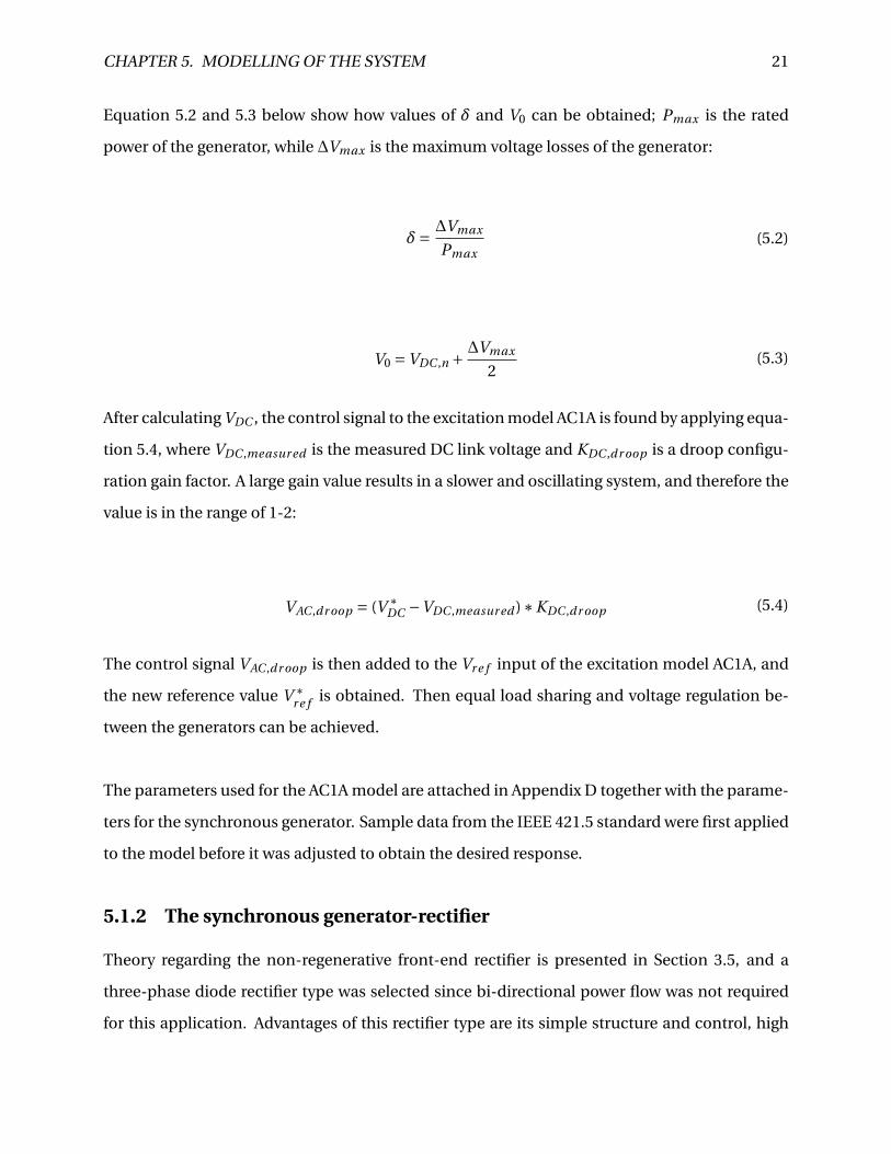
Equation 5.2 and 5.3 below show how values of δ and V0 can be obtained; Pmax is the rated
power of the generator, while ∆Vmax is the maximum voltage losses of the generator:
δ= ∆Vmax
Pmax(5.2)
V0 =VDC ,n + ∆Vmax
2(5.3)
After calculating VDC , the control signal to the excitation model AC1A is found by applying equa-
tion 5.4, where VDC ,measur ed is the measured DC link voltage and KDC ,dr oop is a droop configu-
ration gain factor. A large gain value results in a slower and oscillating system, and therefore the
value is in the range of 1-2:
VAC ,dr oop = (V ∗DC −VDC ,measur ed )∗KDC ,dr oop (5.4)
The control signal VAC ,dr oop is then added to the Vr e f input of the excitation model AC1A, and
the new reference value V ∗r e f is obtained. Then equal load sharing and voltage regulation be-
tween the generators can be achieved.
The parameters used for the AC1A model are attached in Appendix D together with the parame-
ters for the synchronous generator. Sample data from the IEEE 421.5 standard were first applied
to the model before it was adjusted to obtain the desired response.
5.1.2 The synchronous generator-rectifier
Theory regarding the non-regenerative front-end rectifier is presented in Section 3.5, and a
three-phase diode rectifier type was selected since bi-directional power flow was not required
for this application. Advantages of this rectifier type are its simple structure and control, high

CHAPTER 5. MODELLING OF THE SYSTEM 22
energy efficiency and performance of the input factor. For this system, the voltage regulation
was conducted in the excitation system of the generator, and the rectifier did not need to con-
trol the voltage. [23] The rectifier is modelled with a six-pulse three-phase diode rectifier from
the Simscape library, which consists of three bridge arms with two diodes each. [16] The idea
was to use the “Average-value Rectifier” block from the Simscape library for faster simulations
and less disturbance in the transient and steady states. However, simplifications in the block
resulted in errors during simulation with generator sets in parallel, and the simulation ended.
The rectifier block from the Simscape library was therefore selected, and the simulations then
operated correctly. However, because of greater harmonics from the rectifiers, filters were em-
ployed to filter out the harmonics for the controller and the results. The filters applied were the
low-pass filter and the “Mean” block from the Simulink library. The mean block calculates the
mean value of the input signal. [15]
5.2 Gas engine
The engine connected to the generators is a gas engine with LNG as the fuel source. By using
LNG instead of diesel, the sulphur oxide emissions are reduced by 90–95 %, while carbon diox-
ide can see a reduction of 20–25 %. [30] In Simulink, the engine was modelled with a speed
governor and the gas turbine model GAST to simulat the gas engine dynamics. The GAST model
is further described in "Gas Turbine Control for Islanding Operation of Distribution Systems"
by Pukar Mahat, Zhe Chen and Birgitte Bak-Jensen. [43] As mentioned in Section 3.1, voltage
regulation and power sharing are controlled in the excitation system of the synchronous gener-
ator. Therefore, the governor and turbine model control the speed reference and thus also the
fuel flow of the engine. When the generator regulates the DC voltage, the governor changes the
speed to correspond to the requirements in order to obtain the DC voltage on the DC link. The
model was created with fixed and variable speed, and the variable speed was modelled with an
equivalent function from the load limit curve of the gas engine with respect to speed and active
power.

CHAPTER 5. MODELLING OF THE SYSTEM 23
5.2.1 Gas turbine model (GAST)
The dynamics of the gas engine were simulated with the GAST model, shown in Figure 5.4, which
is one of the most commonly used dynamic models because of its simplicity. [43] A general gas
turbine consists of three parts: an axial compressor, a combustion chamber and a turbine. In
the combustion chamber, the fuel and compressed air from the axial compressor are mixed, and
the combustion process occurs. The real work on the turbine shaft is produced in the turbine
when the hot gas is isentropically expanded. Then, the working fluid (air) is cooled down with
constant pressure between the compressor and the turbine to maintain the temperature limits.
[36]
In the GAST model from Figure 5.4, T1 is the controller time constant, while T2 is the fuel sys-
tem time constant. The loop back to the low value gate is the temperature control loop, where
T3 is the load limiter time constant, KT is temperature control loop gain and AT is the ambient
temperature load limit. The temperature control loop interacts with the fuel system when the
control signal from the loop is smaller than the control signal from the speed governor, and thus,
the injection is adjusted so that the engine does not overheat; DTur b is the frictional losses of the
turbine, but this factor was neglected for the simulations (0). [43] The parameters of the turbine
model GAST used for the simulations are attached in Appendix D and were chosen from Pukar
Mahat, Zhe Chen and Birgitte Bak-Jensen’s article. [43]
Figure 5.4: Block diagram of GAST turbine model

CHAPTER 5. MODELLING OF THE SYSTEM 24
5.2.2 Speed governor
A conventional method for controlling the load sharing between generator sets is speed droop,
in which the governor reference speed increases when the load decreases to accomplish stable
operation. [43] For the power system with the DC link, the excitation system of the synchronous
generator controls the load sharing, through DC droop as mentioned in Section 5.1.1. Then, the
governor controls the speed reference and the fuel injection to the GAST turbine with reference
from the excitation system. In this way, an increase in load leads to lower voltage on the DC link,
so the excitation system indicates to the field windings of the generators to increase the cur-
rent produced in order to maintain the required power production. The governor with a slower
regulation than the excitation system then detects the need for current to field windings and
increases the fuel injection to meet the demand. The speed drops, which signals to the GAST to
increase the mechanical power to accomplish stable operation. The block diagram of the speed
governor is presented in Figure 5.5.
The governor is an isochronous controller, where the speed is regulated towards the reference
speedωr e f through a PI-controller. The parameters of the PI-controller, Kp,ω and Ti ,ω are based
on same parameters as the GAST model. [43]. The reference ωr e f is equal to 1 for the system
when simulating with fixed speed. One of the advantages of using LVDC is the possibility that
the gas engine could work on variable speeds to minimise the energy consumption and adapt
to the load at a given time, which cannot be obtained with fixed speed reference to the speed
governor.
Figure 5.5: Block diagram of the speed governor with fixed speed (ωr e f = 1)
CHAPTER 5. MODELLING OF THE SYSTEM 25
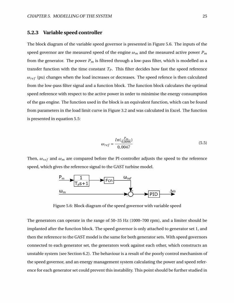
5.2.3 Variable speed controller
The block diagram of the variable speed governor is presented in Figure 5.6. The inputs of the
speed governor are the measured speed of the engine ωm and the measured active power Pm
from the generator. The power Pm is filtered through a low-pass filter, which is modelled as a
transfer function with the time constant TP . This filter decides how fast the speed reference
ωr e f (pu) changes when the load increases or decreases. The speed refence is then calculated
from the low-pass filter signal and a function block. The function block calculates the optimal
speed reference with respect to the active power in order to minimise the energy consumption
of the gas engine. The function used in the block is an equivalent function, which can be found
from parameters in the load limit curve in Figure 3.2 and was calculated in Excel. The function
is presented in equation 5.5:
ωr e f =ln( Pm
0,0096 )
0,0047(5.5)
Then, ωr e f and ωm are compared before the PI-controller adjusts the speed to the reference
speed, which gives the reference signal to the GAST turbine model.
Figure 5.6: Block diagram of the speed governor with variable speed
The generators can operate in the range of 50–35 Hz (1000–700 rpm), and a limiter should be
implanted after the function block. The speed governor is only attached to generator set 1, and
then the reference to the GAST model is the same for both generator sets. With speed governors
connected to each generator set, the generators work against each other, which constructs an
unstable system (see Section 6.2). The behaviour is a result of the poorly control mechanism of
the speed governor, and an energy management system calculating the power and speed refer-
ence for each generator set could prevent this instability. This point should be further studied in

CHAPTER 5. MODELLING OF THE SYSTEM 26
the future; however, it gives an indication of how the variable speed generators could operate.
5.2.4 Calculation of SEC
The SEC of an engine is explained in Section 3.2 with a load limit curve of a gas engine. To cal-
culate the SEC for different load outputs of the generator sets, two Matlab scripts were created.
The first script calculates the SEC for generator sets with variable speed generator sets, and the
inputs of the function are the measured speed levels of the generator in rpm and the speed and
consumption reference points from the load limit curve in Figure 3.1. The function calculates
the SEC along the load limit curve, and a linear equation for the plotting is assumed. For the
calculations with fixed speed, the speed measurements and speed reference points are replaced
with the measured active power and output power from the figure. Subsequently, the calcula-
tions follow the green line from the figure with a reference speed of 1000 rpm. The plots from
the two cases were then plotted in Matlab, and the results are further discussed in Chapters 6
and 7. The Matlab scripts are attached in Appendix B.
5.3 Energy storage system
The energy storage system used for this power system is a lithium-ion battery connected to the
DC link through a bi-directional DC/DC converter, which ensures a bi-directional power flow.
To model the converter, dynamic average modelling is used since exact switching behaviour
is not required. The converter is used for power management of the battery. A simple bat-
tery model from the Simscape library was implanted to simulate the battery. [13] The battery
calculates the SoC during operation and the charge/discharge power of the controller for the
bi-directional converter.
5.3.1 Modeling of the Bi-directional DC/DC converter
For the system simulations in Simulink, a non-isolated bi-directional converter was implemented.
The benefits of the non-isolated type compared to the isolated type are higher efficiency, size,
weight and cost. Based on the theory from Section 3.4, buck mode and boost mode are applied
CHAPTER 5. MODELLING OF THE SYSTEM 27
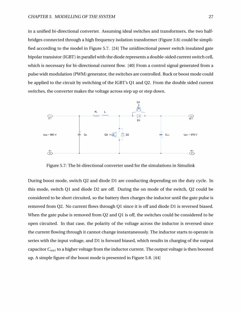
in a unified bi-directional converter. Assuming ideal switches and transformers, the two half-
bridges connected through a high frequency isolation transformer (Figure 3.6) could be simpli-
fied according to the model in Figure 5.7. [24] The unidirectional power switch insulated gate
bipolar transistor (IGBT) in parallel with the diode represents a double-sided current switch cell,
which is necessary for bi-directional current flow. [40] From a control signal generated from a
pulse widt modulation (PWM) generator, the switches are controlled. Buck or boost mode could
be applied to the circuit by switching of the IGBT’s Q1 and Q2. From the double sided current
switches, the converter makes the voltage across step up or step down.
Figure 5.7: The bi-directional converter used for the simulations in Simulink
During boost mode, switch Q2 and diode D1 are conducting depending on the duty cycle. In
this mode, switch Q1 and diode D2 are off. During the on mode of the switch, Q2 could be
considered to be short circuited, so the battery then charges the inductor until the gate pulse is
removed from Q2. No current flows through Q1 since it is off and diode D1 is reversed biased.
When the gate pulse is removed from Q2 and Q1 is off, the switches could be considered to be
open circuited. In that case, the polarity of the voltage across the inductor is reversed since
the current flowing through it cannot change instantaneously. The inductor starts to operate in
series with the input voltage, and D1 is forward biased, which results in charging of the output
capacitor Cout to a higher voltage from the inductor current. The output voltage is then boosted
up. A simple figure of the boost mode is presented in Figure 5.8. [44]

CHAPTER 5. MODELLING OF THE SYSTEM 28
Figure 5.8: Simplified topology of the boost mode. Source: [24]
In the second operation buck mode, Q1 and D2 conduct depending on the duty cycle, while
Q2 and D1 are off. When Q1 is on and Q2 is off, the inductor and capacitor Cout are charged
from the DC-link with higher nominal voltage than the battery side. Consequently, Q1 is turned
off, and the current from the inductor is discharged through D2 because the inductor current
cannot change instantaneously, which results in a lower voltage across the load, stepped down.
The buck mode of the operation is shown in Figure 5.8. [44]
Figure 5.9: Simplified topology of the buck mode. Source: [24]
5.3.2 Converter parameters
In an electrical system, the battery energy storage is an expensive part. Parameters like switch-
ing frequency, filter capacitor and inductor should therefore be carefully selected to reduce bat-
tery aging. When considering battery aging, heat development is a regular source of this mat-
uration, and with higher internal losses, the heating increases. [57] One source of higher losses
is skin and proximity effects from high switching frequency (5–20 kHz), which results in higher
internal impedance. A reason for the skin effects is battery current ripple. In Sven De Breucker’s
report “Impact of DC-DC converters on Li-ion Batteries”, the current ripple could not be associ-
ated with aging of the battery. However, current ripple impacts the battery management system,
and may cause the cells to exceed the maximum voltage limit. [55] To prolong the life time of the
battery, small ripples in voltage and current are recommended from supplier. For the system in
this master’s thesis, ∆i = 5% of the rated Ah capacity, while ∆Vbat = 5%. [57]

CHAPTER 5. MODELLING OF THE SYSTEM 29
For the IGBT, high switching frequency results in higher losses, shorter battery life and higher
operation temperatures. Simulation run time is also slower with higher switching frequency
since the sample time needs to be reduced. The switching frequency for the IGBT was selected
to be 3 kHz, then the simulation time is sufficient. With the lower switching frequency, dynamic
response of the converter controllers can be reduced. [11] In Table 5.1, the selected converter
parameters are presented. The calculations for the parameters are included in Appendix A.1.
The charging conductor L and smoothing capacitor Ci n were calculated from equation 5.6 and
5.7. [48] To reduce voltage and current ripples, the output capacitor is dimensioned during sim-
ulations.
Ci n = ∆iL
8 fs∆VB at(5.6)
L = ∆VB at (1−D)
fs∆iL(5.7)
Table 5.1: Parameters for converter calculationsfs 3000 H z
Ci n 20 mFCout 59,259 µF
L 0,361 mHRon 1,5 mΩ
5.3.3 Control system for the bi-directional converter
For this study, two different control methods are investigated. The first method investigated is
load sharing with droop control of the battery, and the second control method is peak shaving
from the battery. Both control methods consist of a cascade controller with an outer and inner
control loop. The inner loop is the same for both methods, and it controls the inductor current
iL by supplying a reference to the duty ratio d. For the load sharing method, the output voltage

CHAPTER 5. MODELLING OF THE SYSTEM 30
of the DC link is controlled by the outer loop, which gives the current reference i∗L to the inner
loop. [57] During peak shaving, the outer loop compares the load current with the generator
currents to avoid the generator sets supplying the peak load. [32] The outer loop delivers the
current reference i∗L for peak shaving to the inner loop.
By applying the averaged switch modelling to the circuit from Section 5.3.1, a unified equiva-
lent circuit is obtained. During buck and boost mode, the current only changes direction, which
provides ddi schar g e = dchar g e . [24] From the equivalent circuit in Figure 5.10, the system be-
haviour of the converter can be studied in order to select the controller parameters.
Figure 5.10: Equivalent circuit of the bi-directional DC/DC converter. Source: [24]
From Figure 5.10, the general averaging model is developed into equations 5.8 and 5.9. An ex-
planation of these equations is presented in Appendix A.2. In equations, D is the stationary
duty ratio (D =Vbat /VDC ), while d is the duty ratio. [41] In Figure 5.11, the block diagram of the
cascaded converter controller is presented.
Ci n = ∆iL
8 fs∆VB at(5.8)
L = ∆VB at (1−D)
fs∆iL(5.9)

CHAPTER 5. MODELLING OF THE SYSTEM 31
Figure 5.11: Block diagram of the cascade controller. Source: [57]
Inner control loop (Current controller)
To develop the inner current controller of the cascade controller, equation 5.8 must be adapted
so the real variable t is converted to the complex variable s by applying the Laplace transform.
The result is in equation 5.10 presented, and the calculations can be found in Appendix A.3.
IL = dVDC −VB at
RL( LRL
)s +1(5.10)
The control signal from the current controller is represented with the duty ratio d from equation
5.10. With the feed-forward coupling of the measured VDC and VB at and the formula for the duty
ratio d, IL is simplified to equation 5.11. The derivation and the block diagram of the explanation
is attached in Appendix A.3.
IL = 1
RL
Hc,i (s)e
( LRL
)s +1(5.11)
When constructing the controller of the converter, the time constant must be accounted for.
For the switching period or the time delay in the PWM converter, TSW is calculated from the
switching frequency TSW = 1/ fSW . For the block diagram, the switching is represented by a
first-order time delay, as can be seen in Figure 5.12. The second time delay considered is the
measurement delay in the simulation, which is connected in a feedback loop. The time delay
equals 1/3 of TSW . [52]

CHAPTER 5. MODELLING OF THE SYSTEM 32
Figure 5.12: Control loop when disturbances from VB at has been eliminated. Source: [57]
The regulator selected for the regulation of the inductor current (IL) is a PI-controller. The cur-
rent controller is tuned with the modulus optimum design criterion. The calculations and ex-
planations are included in Appendix A.3. In Table 5.2, the control parameters of the current
controller are presented.
Table 5.2: Parameters for the inner current controller.Ti ,i Kp,i TSW Tmeas
0.241 0.41 0.33 ms 0.11 ms
Outer control loop (Voltage controller)
The outer loop of the cascade controller controls the DC link voltage and the reference current
for the current controller. To develop an expression for the output voltage from the inductor
current, the Laplace transform was applied to equation 5.7, and then equation 5.12 is developed
as follows:
VDC = D IL
Cout s(5.12)
For the design of the voltage controller, RLP is set to infinity to simulate no-load condition. Then,
the expression in equation 5.12 is reduced to an integral term, as seen in equation 5.13.
VDC = D IL
Cout s(5.13)

CHAPTER 5. MODELLING OF THE SYSTEM 33
The block diagram of the voltage controller is next developed from the equation, with a time
delay from the inner current loop and the PI-controller as seen in Figure 5.13. By applying rea-
sonable simplification to the current loop, RLP and the inner current loop are considered to
follow imposed references, and the current loop can then be simplified to a first-order time de-
lay. The dominant pole of the load can be cancelled by adjusting the integral time constant of
the PI-regulator in the current controller equal to the load. The time constant of the time delay
is then three times higher than the system sampling time (Ts). For this study, the time constant
of the current controller was selected to be 15 times higher than the sampling time to improve
the disturbance rejection capability. [25]
Figure 5.13: Voltage loop with imposed references. Source: [57]
Then, the voltage controller can be tuned by using the symmetrical optimum criterion. The re-
sults are in Table 5.3, while the calculations for this section are in Appendix A.3. The parameters
for the controller in the inner and outer loop are the same for both control methods.
Table 5.3: Parameters for the outer voltage controller.Ti ,o Kp,o TSU M
0.02 1.625 5 ms
5.3.4 Droop control
With the droop control configuration, the DC link voltage is controlled by droop control of the
battery and the generator sets; droop control of the generator sets is explained in Section 5.1.1.
The load sharing between the sources is obtained when the voltage drops according to the droop
factor, as expressed in Figure 5.14. [47] The concept of the battery droop control is that at the idle

CHAPTER 5. MODELLING OF THE SYSTEM 34
voltage reference (V0,bat ), the battery does not absorb or deliver power to the system. When a
load change occurs, the voltage increases or decreases depending on whether the load increases
or decreases. In Figure 5.14, the load is increased from a level P1 to P2. Then, V0,bat drops
towards V2 and supplies PB at to the system together with the power from the generator sets.
The amount of power absorbed or supplied from the battery is decided from the battery droop
factor δB at . [57]
Figure 5.14: Battery droop control during increase of load. Source: [57]
Mathematically, the share of power between the battery and the generator set could be obtained
by solving equations 5.14, 5.15 and 5.15, where V0,G1 and V0,G2 are the terminal voltage reference
for the two generator sets. They are constants of the equation together with the total load power
PLoad , the battery voltage reference V0,B at and the droop factors; δG1 and δG2 are the droop
factors for the generator sets and were selected to be 0.05. (see Section 5.3.3) For this thesis, the
simulations were tested with an δB at = 0.05 . The equations do not offer a precise visualisation
of the load sharing because of distortion of the DC link voltage and delays. However, it offers an
indication of how the system reacts. [57]
PG1δG1 −PG2δG2 =V0,1 −V0,2 (5.14)
PG2δG2 −PB atδB at =V0,2 −VB at (5.15)
PG1 +PG2 +PB at = PLoad (5.16)

CHAPTER 5. MODELLING OF THE SYSTEM 35
For the battery droop controller, a block that calculates the DC voltage reference V0,DC is im-
planted in the controller for the bi-directional DC/DC converter, and V0,DC is compared with the
measured DC link voltage to give the control voltage V ∗DC to the outer loop of the cascade con-
troller, as explained in Section 5.3.3. Then, the battery and generator sets share the load after the
droop of each controller, as represented in Figure 5.14 and the equations above. The block dia-
gram of the battery droop controller implanted is shown in Figure 5.15. The time constant TB at
of the low-pass filter regulates the speed of V0,B at towards the DC link voltage. Consequently,
TB at was selected to be 0.02 for faster regulation from the battery. With large TB at , V0,B at moves
more slowly towards the DC link voltage compared with a small factor. [57]
Figure 5.15: Block diagram of the droop controller implanted in Simulink
5.3.5 Peak shaving control
For the peak shaving controller, the intention is to avoid the generator sets to supply the peaks
of the variable load for the system and then ensure the smother operation of the generator sets.
Smother operation of the generator sets indicates that they operate at a more constant power
contribution, since the battery absorbs or supplies power to the system after a load change oc-
curs. If the load drops, the battery absorbs power from the system, and the generator sets do
not need to reduce the production to a minimum. The amount of power absorbed or supplied
by the battery is determined by the battery management system with respect to SoC and charg-
ing/discharging limits. [28] Energy storage capacity, maximum charge and discharge power and
the load characteristics of the battery decide the peak power the battery can produce. [32] An
example of the peak shaving control method is presented in Figure 5.16.

CHAPTER 5. MODELLING OF THE SYSTEM 36
Figure 5.16: Principal diagram of the peak shaving control method
The control block for peak shaving is shown in Figure 5.17. The block supplies the desired charg-
ing and discharging current (Ir e f ) to the inner current loop from Section 5.3.3. The current refer-
ence is given by a low-pass filter, where the input is the total current from the system (ILoad ) and
calculated from the measured battery and generator sets current. Furthermore, ILoad is then
compared with the generator set currents to give the charging/discharging current to the con-
troller. The PI-controller has the same parameters as calculated in Section 5.3.1. The low-pass
filter is modelled as a transfer function with the time constant TLoad , and it regulates the rate
at which ILoad moves against the current from the generator sets. With a large time constant,
ILoad diverges from the generator current for a longer period, which gives a more used battery.
Then, the generator sets have a slower contribution to the load demand, while the battery takes
more of the peak power. [56] The transfer function with the time constant TGen , is a low-pass
filter with a low time constant, which filters out disturbances from the measurements. A current
limiter is placed behind the PI-controller to ensure that the charge and discharge currents do
not surpass limits from the battery supplier (2.8kA- (-2.8kA)).
Figure 5.17: Block diagram of the peak shaving controller implanted in Simulink

CHAPTER 5. MODELLING OF THE SYSTEM 37
5.4 Limitations and evaluation of Chapter 5
On a real system, the propulsion engines and hotel loads are connected on the DC link through
inverters. However, for this system, the load was modelled with a variable resistor on the DC
link. Since the resistor load depends on the voltage and active power, the load somewhat de-
viates from the reference when the voltage changes according to the droop factor. The system
does not have an AC load side and is limited to one DC link, such that the generator sets and
battery supply power through rectifiers and a bi-directional DC/DC converter. The six-pulse
rectifier connected to the generator sets create harmonics in the system, which are reduced
through filters. Investigating the harmonics could be a new task for future studies to evaluate if
they violate requirements and how they could be reduced. To use the “Average-value Rectifier”
block from the Simscape library, the simplifications of the block should be investigated. Another
option could be to implant an energy management system (EMS) for the reference values to the
control systems, the output of the rectifier is then controlled through an EMS system instead of
directly to the excitation system and governor system.
The governor controller for variable speed is limited to a common governor, which gives the
same reference speed to the generator sets. This “locks” the production of the generator set
to the same speed reference and removes the opportunity for the generator sets to operate at
different load levels. This option could lead to instability or oscillations in the signal. When
installing speed governors to each generator set, they start to operate against each other and
create an unstable system. The reference speed to the generator sets should be calculated from
an EMS system or the AC load side, instead of the active power produced from the generator
sets. However, since the system is limited to only a load on the DC link, the only speed reference
the system has is from the generator sets on the AC side of the rectifiers.

6 | Testing of the model
To determine how the Simulink model and control system (explained in Chapter 5) responded
and operated, the models was tested with a load change and with one generator set dropped out
of the system. The load change is presented in Figure 6.1, and the constant load when generator
set 2 was disconnected is 2300 kW. The load was modelled with a variable resistance, such that
the resistance was calculated from the DC link voltage and the desired load power. The testing
shows how the control system reacts and if the system is stable and has redundancy. Some pa-
rameters may be changed to obtain a stable system. All of the plots for this chapter and Chapter
7 were plotted in Matlab.
Figure 6.1: Applied load change
6.1 One generator set
For the simulations with one generator set connected, the load scenario from Figure 6.1 was
simulated with the option of fixed speed and variable speed. After the change in load, the goal is
to achieve stability and supply the amount of needed power without violating the voltage limits
explained in Chapter 4.
38

CHAPTER 6. TESTING OF THE MODEL 39
The DC link voltage for constantωr e f reached a steady state after 5-6 seconds, while for the sce-
nario with variableωr e f the system used 10 seconds and produced higher fluctuations from the
load change. This distinction is because the change in speed gives a slower response in power
production for the variable speed generators than the fixed speed generators. To compensate
for the slower response, a faster speed governor could be used or a battery could be implanted
in the system, thus reducing the load change for the generator. The DC link voltage is presented
in Figure 6.2. As mentioned in Chapter 4, the voltage variations should operate within ± 10 % of
system voltage. For a safety margin, this system is modelled to obtain the voltage limits between
900–1000 V. To accelerate the response, the gain of the speed controller could be increased.
Figure 6.2: DC link voltage with fixed and variable speed
As seen in Figure 6.3, the DC link voltage drops when the load increases, and the amount is de-
cided by the controller explained in the previous chapter. Ripples on the red line (variable speed
controller) are higher than for the blue line with the fixed speed controller. This variation could
be because the PI-controller is not tuned optimally (to high proportional gain) and that theωr e f
should be calculated from another source than the active power produced by the generator.
Figure 6.3: Power flow during load increase

CHAPTER 6. TESTING OF THE MODEL 40
In Figure 6.4, the reference and measured speed of the two cases are visualised. Blue is the fixed
speed, while red is the variable speed. In the case with the variable speed controller, the speed
follows the reference speed calculated from the optimal speed function and operates at a lower
speed when the load is reduced.
Figure 6.4: Speed of the engine for fixed and variable speed
6.2 Two generator sets
When two generator sets are connected to the same load, as explained in Section 6.1, the vari-
able speed governor needs 30 seconds to reach a steady state. It gives a high overshoot during
the load change, as seen from Figure 6.5. The high overshoot is also found in the active power
production in Figure 6.6, and it is a result of the speed deviation at the start of the simulation.
Figure 6.5: DC link voltage with fixed and variable speed, two generator sets
The generator sets produce the same amount of power to the system because of equal con-
trol parameters. The load change is relatively small compared to the installed power (∆PL =200kW ), so the system with the fixed speed reaches the new steady state fast (4-5 s) without
much fluctuation. The system may have reached steady state a bit to quickly compared with

CHAPTER 6. TESTING OF THE MODEL 41
real-life situations, and a slower result could be obtained by increasing the governor values.
Figure 6.6: Power flow with fixed and variable speed, two generator sets
The measured and reference speed during the load case are presented in Figure 6.7, in which
the red line indicates the system with variable speed. The cause of the oscillations in the first
15 seconds in Figure 6.6 is the deviation between the measured speed (dotted) and reference
speed (bold). The PI-controller was un able to control the measured speed towards the reference
speed when the starting load was as low as in the figure. At the beginning of each simulation,
the speed of the engine began at 1 pu, which led to a drop in 0.3 pu of the reference speed when
the load is at 800 kW. The PI-controller is not fast enough to compensate for the difference in
the beginning of the simulation, even though the proportional gain was increased five times.
When the load was increased or the system was simulated for 30 seconds, the system reached
a steady sate (see Figure C.1 in Appendix C.1). At higher start loads, the same problem did not
occur. A solution for the system is to increase the proportional gain of the PI-controller in the
speed governor; however, this option led to high ripples in the signal, as seen in Figure C.3 in
the Appendix. Another solution could be to have the start speed on the engine at a lower level
or start the simulation when the system reaches a steady state, since the controller operates
acceptably after the first 30 seconds.

CHAPTER 6. TESTING OF THE MODEL 42
Figure 6.7: Engine speed with fixed and variable speed, two generator sets
For the next simulations, generator set 2 was disconnected from the system after 15 seconds.
Then generator set 1 had to supply the load on 2300 kW without becoming unstable. In Figure
6.8, the DC link voltages for fixed (blue) and variable speed (red) are presented. The source
of the overshoot from the variable speed is the same as explained earlier in this section. Both
control methods reached a steady state after generator set 2 was disconnected, and the fixed
speed generator reached steady state before the variable speed generator.
Figure 6.8: DC-link voltage with fixed and variable speed, during loss of gen set
The active power production is presented in Figure 6.9, in which the variable speed generators
used 10 seconds to reach steady state, while the fixed speed generators used 7 seconds to reach
steady state. The next step was to connect the battery to the system and simulate the same load
scenario.

CHAPTER 6. TESTING OF THE MODEL 43
Figure 6.9: Power flow with fixed and variable speed, during loss of a gen set
6.3 Two generator sets and battery
For the simulations in this section, only the fixed speed generators were simulated together
with the battery. The control methods for the simulations are peak shaving and load sharing, as
described in Section 5.3. The load was increased from 2300 kW to 4480 kW after 15 seconds.
6.3.1 Load sharing
During load sharing, the droop control explained in Chapter 5 determines the amount of power
shared between the generator sets and the battery. The generator sets produce the same amount
of power since the droop slope is equal. The power flow is presented in Figure 6.10, which shows
that the system reached steady state after 7 seconds. To increase the amount handled by the
battery, the δB at could be decreased.

CHAPTER 6. TESTING OF THE MODEL 44
Figure 6.10: Power flow with droop control during a load increase
In Figure 6.11, the DC link voltage during the load change is presented. The voltage stabilised
around 940 V after 6–7 seconds with some ripples on the signal. The ripples stemmed from the
electronic converters in the system that generated harmonic voltages. To reduce the harmonics
into the AC network, harmonic filters or voltage regulators could be used. On the DC side, the
harmonic levels are minimised by the capacitor. Basic DC loads like motor or transmission lines
with high inductive impedance operate as filters, and the harmonics are therefore of less im-
portance on the DC side. [54] The harmonics were around 0.5%, which is acceptable compared
with the voltage tolerance limits from Chapter 4 (max. 10 %).
Figure 6.11: DC link voltage with droop control during a load increase
For the next simulation, generator set 2 is disconnected after 15 seconds when the total load is
3000 kW. Generator set 1 and the battery share the remaining load with the goal of obtaining the

CHAPTER 6. TESTING OF THE MODEL 45
load supply. The power flow is presented in Figure 6.12, in which the load drop of 100 kW after
the loss of generator set 2 can be seen. The voltage dropped to compensate for the load increase
on generator set 1 and the battery and was unable to rise to 3000 kW. The reduced load power is
a result from the lower DC link voltage.
Figure 6.12: Power flow with droop control during loss of gen set 2
If the power supplied by the battery is increased, generator set 1 and the battery could ensure
redundancy up to 5 kW loads until the SoC reach 60 % (2330kW +2500kW for 4.5 min, calculated
from equation 3.1).
6.3.2 Peak shaving
During peak shaving, the battery contributed more power to the system when a change oc-
cured than in the load sharing scenario, as seen from Figure 6.13. The regulation in the battery
controller was faster than in the generator sets so that the battery supplied the peak, while the
generator sets operated slower and supplied the remaining load. After a load change, the load
current and generator current in the controller operated towards each other, which reduced the
reference current to the inner current loop. This trend can be seen after 13 seconds in the figure,
at which point the battery power is decreasing, and the generator power is increasing.

CHAPTER 6. TESTING OF THE MODEL 46
Figure 6.13: Power flow with droop control during a load increase
To reduce the amount of battery power delivered and remove the sudden drop, the proportional
gain of the PI-controller should be increased compared to the integral gain and the time con-
stant TLoad should be reduced. In Figure 6.14, the proportional gain Kp increased while TLoad
reduced to 0.02 s (Kp = 5,Ki = 1). The load current moved slowly toward the generator current
compared to the previous figure, and a smoother transition was obtained. These parameters
were used for the rest of the simulations with peak shaving.

CHAPTER 6. TESTING OF THE MODEL 47
Figure 6.14: Power flow with droop control during a load increase (Kp = 5,Ki = 1,TLoad = 0.02)
The ripples on the voltage signal are the same as for the load sharing scenario (Figure 6.11).
The DC link voltage decreased when the generator set started to increase, as seen at the 10–15
second point in Figure 6.15. During peak shaving, the DC link voltage varies more than for load
sharing; however, the drops should be reduced so the DC link voltage operates within 900 to
1000 volts.
Figure 6.15: DC link voltage with droop control during a load increase
When generator set 2 is disconnected from the system, the battery supplies constant power until
generator set 1 reaches steady state. Then, the battery power starts to reduce the power delivery,
and generator set 1 increases the power production. Generator set 2 or the backup generator set
must be reconnected after 4.5 minutes since the battery surpasses 60 % SoC.

CHAPTER 6. TESTING OF THE MODEL 48
Generator set 1 does not have enough installed power to handle the load alone, and it over-
loaded after 50 seconds for this control method.
Figure 6.16: Power flow with droop control during loss of gen set
CHAPTER 6. TESTING OF THE MODEL 49
6.4 Evaluation of Chapter 6
The model was tested for scenarios of a load change and the removal of one generator set from
the system for one generator set and two generator sets with and without battery connected to
the system. The variable speed generators had a slower response than the fixed speed genera-
tors, with the reason being a slower response in power production. The variable speed governor
generated higher ripples in the active power signal and, with two generator sets in parallel, the
signal oscillate. The reasons for this result could be that the controller was not tuned correctly,
and another issue with the controller is how the speed reference is calculated. The reference
speed is calculated from the power produced by the generator, which creates a reference that
is highly dependent on the speed governor. With a fixed speed, the reference is a known vari-
able that does not change accordingly to the load, which results in a quicker and more stable
response. Most of the simulations are therefore modelled with fixed speed. Generating a better
reference speed for the governor should be addressed in further work.
With load sharing between the generator sets and the battery, the system used 6-7 seconds to
reach the steady state. The electronic converters in the system generated harmonic voltages,
which caused ripples on the signals. For the peak shaving method, the system used around
5 seconds to reach a steady state, which mean it was marginally faster than the load sharing
method. The fast controller in the battery reached steady state almost instantaneously, while
reducing the fluctuations on the generator sets production. To increase the speed of the outer
loop of the converter controller, the proportional gain was increased to 5, while the integrating
gain decreased to 1.
In the next chapter, the methods for the simulation of a load profile that exceeds 500 seconds
are explained.

7 | Simulations and results
For this chapter, the simulations of four different cases are presented. The goal of the simula-
tions was to ensure steady operation and fulfill the requirements explained in Chapter 4. An-
other important topic investigated in the simulations was the SEC of the engines, so different
control methods were investigated to find a solution with a low SEC. At the same time, it was es-
sential to ensure the SoC and DoD limits mentioned in Chapter 2 in the simulations to confirm
the estimated life-time of the battery.
The simulations are based on the theory and control methods developed in this thesis. The
load profile simulated is presented in Figure 7.1 and represents one ferry trip. The real ferry trip
takes about 3000 s (50 min); however, the march speed (steady load) was shortened to speed
up the simulation time. This change does not affect the peak shaving case, but it needs to be
discussed for the droop control case. The real load profile is attached in Appendix B.3. The
parameters studied are active power, DC-link voltage, SEC, battery voltage and SoC of the bat-
tery. The results are plotted with Matlab and presented in this chapter. The four cases are listed
below:
• Case 1: Droop control with generator sets
• Case 2: Droop control with generator sets and battery
• Case 3: Peak shaving with generator sets and battery
• Case 4: Variable speed operation during peak shaving
The load was modelled as a variable resistor, in which the resistance was calculated from the
DC link voltage and load power. Since the resistance depends on the DC link voltage, some
50
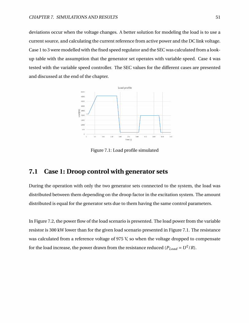
CHAPTER 7. SIMULATIONS AND RESULTS 51
deviations occur when the voltage changes. A better solution for modeling the load is to use a
current source, and calculating the current reference from active power and the DC link voltage.
Case 1 to 3 were modelled with the fixed speed regulator and the SEC was calculated from a look-
up table with the assumption that the generator set operates with variable speed. Case 4 was
tested with the variable speed controller. The SEC values for the different cases are presented
and discussed at the end of the chapter.
Figure 7.1: Load profile simulated
7.1 Case 1: Droop control with generator sets
During the operation with only the two generator sets connected to the system, the load was
distributed between them depending on the droop factor in the excitation system. The amount
distributed is equal for the generator sets due to them having the same control parameters.
In Figure 7.2, the power flow of the load scenario is presented. The load power from the variable
resistor is 300 kW lower than for the given load scenario presented in Figure 7.1. The resistance
was calculated from a reference voltage of 975 V, so when the voltage dropped to compensate
for the load increase, the power drawn from the resistance reduced (PLoad =U 2/R).

CHAPTER 7. SIMULATIONS AND RESULTS 52
Figure 7.2: Power flow for case 1
The DC link voltage presented in Figure 7.3 is in the range of 930–980 V. Before reaching the
steady state after a load change, some small fluctuations occurred, and the system used 10-15
seconds to reach steady state. The ripples on the DC link voltage were highest when the gen-
erator sets produced a total power of 3800 kW. Voltage harmonics were often caused by current
harmonics, which increases at high currents. [9]
Figure 7.3: DC-link voltage for Case 1

CHAPTER 7. SIMULATIONS AND RESULTS 53
7.2 Case 2: Droop control with generator sets and battery
For this case, the amount of power shared between the generator sets and the battery was de-
cided by the droop control method explained in Chapter 5. During the operation, the battery
supplied around 680 kW to the system during marching speed, as seen in Figure 7.4. To ensure
that the SoC limits (80%–65%) were obtained, the SoC used for the marching speed was calcu-
lated with equation 3.1 from Section 3.3. The initial SoC when the marching speed started was
79 %, and the SoC used during the process was 43 %, which resulted in a new SoC at 36 % that
violates the limits from the battery supplier. The battery can operate on these conditions, but
the battery supplier cannot guarantee the life time of the battery when the limitations are vi-
olated. A solution to this issue could an increase in the droop factor in the battery controller,
which could lead to a reduction of the load power contributed from the battery. Installing a bat-
tery with higher energy capacity is another option, and the energy capacity should be around
2900 kWh to deliver 700 kW during the march speed. To increase the battery capacity, a study
around price and space onboard the vessel must be conducted, since the battery is an expen-
sive and complex installation. Equation 7.1 calculates the SoC for the operation, and the other
calculation is based on the same equation.
SOC (t −1) = 700kW
1017kW h∗0,64h (7.1)

CHAPTER 7. SIMULATIONS AND RESULTS 54
Figure 7.4: Power flow for case 2
The charging power from the generator sets during the low load period is too small to ensure
the SoC of the battery at the acceptable limits, as shown in Figure 7.5. In the figure, the battery
capacity is in Ah, with a nominal value of 1280 Ah. The SoC of the battery did not return to the
reference at 80 % at the end of the simulation, which would result in a discharged battery after
a few more trips. This issue might be solved by charging the battery from shore after each trip,
which would ensure a charged battery for each trip. Another solution is to charge the battery
with the available generator power in the system. The battery has the capacity to draw 2542 kW
from the system for charging, so the generator sets can operate at a higher load and operate at
a steadier state with less drop. Since the droop factor decided the amount of power shared, a
separate control strategy for charging must be conducted.
Figure 7.5: SoC of the battery for Case 2

CHAPTER 7. SIMULATIONS AND RESULTS 55
The DC link voltage for the case was in the area of 940–980 V, with ripple values of 0.2 % at
the highest load. When the battery was connected to the system, the DC link voltage operated
closer to the reference voltage of 975 V since the load was shared between three components, as
compared to earlier when only the generator sets produced the load power. The bi-directional
DC/DC converter connected to the battery produced extra harmonics to the system, but the
requirements were fulfilled.
Figure 7.6: DC-link voltage for Case 2
7.3 Case 3: Peak shaving with generator sets and battery
In case 3, the peak shaving controller explained in Chapter 5 was used. The generator sets sup-
ply equal amount of power, while the battery supplies the peak loads, which lead to a slower
response from the generator sets during the load changes. The power flow for the load scenario
is presented in Figure 7.7. The slow response of the time constant TLoad and the PI-controller
decide the amount and shape of battery power supplied or drawn from the system. An increase
in the integral gain of the PI-controller leads to a faster response towards the set point, while a
higher time constant leads to less contribution from the battery. The parameters could be ad-
justed if a smaller or larger battery is installed. With a smaller battery, TLoad should be increased
to reduce the power contributed over time, so the battery can still handle the peaks. With a larger
battery, TLoad should be decreased, and then the battery supplies power to the peaks and con-
tributes over a longer period. In the figure, the time constant is modelled with TLoad equal to
0.02 seconds.
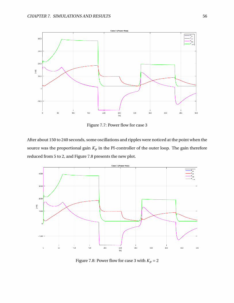
CHAPTER 7. SIMULATIONS AND RESULTS 56
Figure 7.7: Power flow for case 3
After about 150 to 240 seconds, some oscillations and ripples were noticed at the point when the
source was the proportional gain Kp in the PI-controller of the outer loop. The gain therefore
reduced from 5 to 2, and Figure 7.8 presents the new plot.
Figure 7.8: Power flow for case 3 with Kp = 2

CHAPTER 7. SIMULATIONS AND RESULTS 57
The SoC of the battery operated in the area of 1024 Ah (80 %) and 970 Ah (76 %), which indicates
that the battery has stored power available. The SoC of the battery is presented in Figure 7.9. The
battery is dimensioned to discharge and charge up to 2540 kW (2.5C); however, the controller
limits the discharge current to 2000 A (1800 kW). The advantage of the limits is that the gener-
ator sets operate at a level where the energy consumption is lower. Installing a smaller battery
is possible for the case. With a capacity of 720 kWh and the possibility to charge and discharge
2.5C (1800 kWh) the same operation could be obtained with a smaller battery. When the limits
are increased, the battery draws higher charging power from the system, thus reducing the sud-
den drop after the load change occurs. The discharging power from the battery is approximately
equal because of the logic in the controller. Over a longer period of the same marching speed,
the battery power will move towards zero and the SoC will not be particulary affected. The gen-
erator sets can then charge the battery for a longer period to compensate for the extra battery
capacity used.
Figure 7.9: SoC of the battery for Case 3
The DC link voltage of the case is presented in Figure 7.10, where the voltage is in the area of
940–975 volts. Since the generator sets were slower than in case 2, the voltage varies more with
the peak shaving controller. The voltage ripple is around 0.7 %, which offered higher results than
from case 2 with the droop controller. The reason for this difference could be that the battery
delivers a higher amount of power to the system, which increases the harmonics to the DC link.

CHAPTER 7. SIMULATIONS AND RESULTS 58
Figure 7.10: DC link voltage for Case 3
7.4 Case 4: Variable speed operation during peak shaving
The power flow with variable speed generator sets was approximately equal to the power flow
from case 3 with the fixed speed generator sets. The difference between the two is the oscil-
lations on the generator power, which indicates an unstable controller of the variable speed
generators. The controllers suggest how the system could operate with variable speed generator
sets, but this is not an optimal solution with the controller constructed in this thesis.
Figure 7.11: Power flow for case 3

CHAPTER 7. SIMULATIONS AND RESULTS 59
In Figure 7.12, the measured speed and the reference speed to the speed governor are presented.
The high gain factors in the speed governor ensure that the engine follows the reference speed
calculated from a look-up table with regard to the given power of the generator set. The high
gain factors may have caused extra oscillations in the signal. The speed limits in the governor
are regulated from the gas engines limits instead of the synchronous generator limits. The limits
for the synchronous generator are 1 to 0.7 pu, and the reason for using the gas engine limits is to
see the difference between fixed and variable speeds with maximum exploitation of the engine.
Figure 7.12: Speed of the gas engine
The advantage of the variable speed opportunity is that the generator set could vary the speed
according to the optimal loading rate. As seen from Figure 7.13, the energy consumption is
lower for the variable speed compared to the fixed speed generator sets. Using the gas engine
limits compared to the synchronous generator limits does not affect the consumption for this
case, since the SEC is at maximum when the speed of the gas engine is 0.6 pu. The SEC is further
discussed in the next section for all of the cases with fixed and variable speed opportunities.
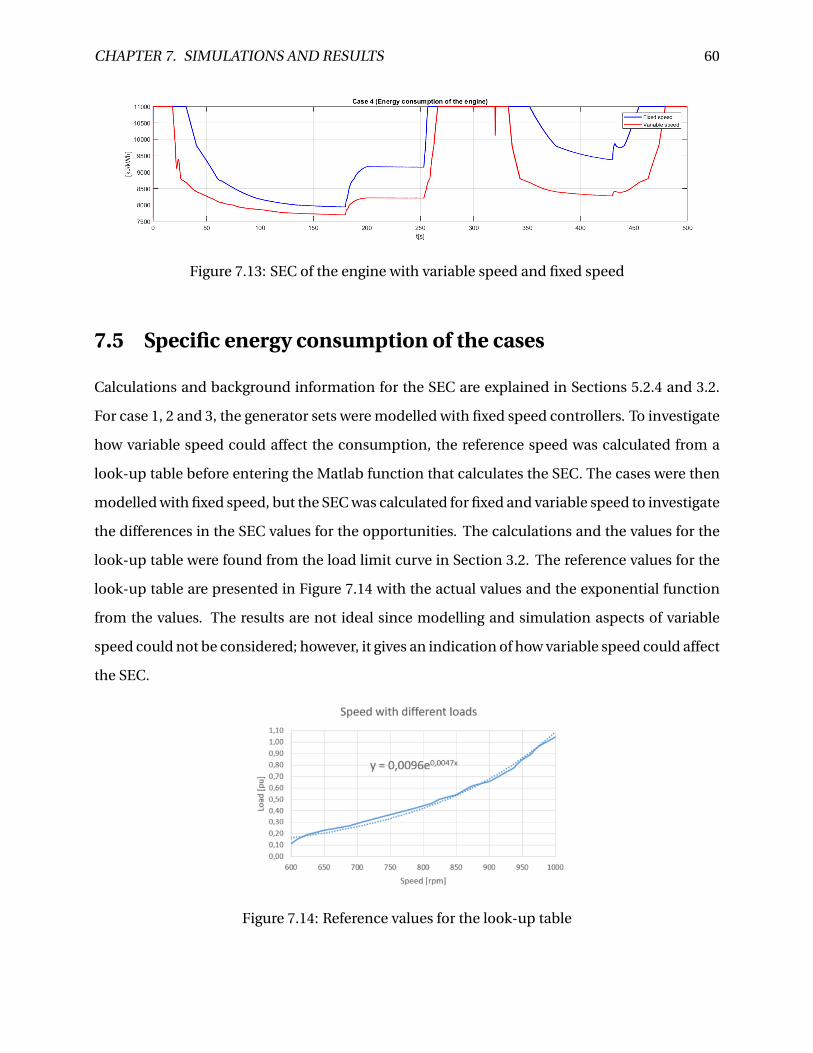
CHAPTER 7. SIMULATIONS AND RESULTS 60
Figure 7.13: SEC of the engine with variable speed and fixed speed
7.5 Specific energy consumption of the cases
Calculations and background information for the SEC are explained in Sections 5.2.4 and 3.2.
For case 1, 2 and 3, the generator sets were modelled with fixed speed controllers. To investigate
how variable speed could affect the consumption, the reference speed was calculated from a
look-up table before entering the Matlab function that calculates the SEC. The cases were then
modelled with fixed speed, but the SEC was calculated for fixed and variable speed to investigate
the differences in the SEC values for the opportunities. The calculations and the values for the
look-up table were found from the load limit curve in Section 3.2. The reference values for the
look-up table are presented in Figure 7.14 with the actual values and the exponential function
from the values. The results are not ideal since modelling and simulation aspects of variable
speed could not be considered; however, it gives an indication of how variable speed could affect
the SEC.
Figure 7.14: Reference values for the look-up table

CHAPTER 7. SIMULATIONS AND RESULTS 61
The SEC values for case 1, 2 and 3 with fixed and variable speeds are presented in Figure 7.15,
in which the dotted line is the fixed speed, while the bold line is the consumption with variable
speed. The figure only presents the consumption from generator set 1, and the assumption is
that the generator sets has the same consumption. Cases 3 and 4 have the same consumption
because the function presented in Figure 7.14 was used as the reference for the speed gover-
nor for the variable speed. Therefore, case 4 is presented in this section together with case 3.
The consumption was lower with variable speed in all of the cases. The highest difference was
found in the area in which the load power was around 2000 kW. For case 2, the consumption was
around 1300 kJ/kWh lower with variable speed generator sets compared to the ones with fixed
speed. At the low load period, the consumption was equal for both opportunities. The differ-
ence in consumption for the opportunities is largest in the middle of the load limit curve, at the
point when the engine operates away from the optimal loading rate and the SEC has the largest
increase compared to the fixed speed reference curve. For example, with an output power of
1000 kW with the fixed speed generator set, the SEC is around 8600 kJ/kWh, while the variable
speed generator set operating at a speed of 800 rpm can produce the same amount of power
with an SEC of 8200 kJ/kWh.
Figure 7.15: SEC of the engine during case 1, 2 and 3 with variable and fixed speed

CHAPTER 7. SIMULATIONS AND RESULTS 62
The mean value of the SEC was calculated in Matlab from the Simulink results and is presented
in Table 7.1 together with the mean value of the active power produced by generator set 1. It
is assumed that generator set 2 produced the same values. The peak shaving method in case
3 resulted in the lowest SEC, while case 2 created the highest. A high average produced power
resulted in lower SEC since the generator sets operate at a more optimal loading rate of the load
limit curve. The cases with the battery connected to the system had the greatest advantage from
operating with variable speed. When the system operated without the battery connected, the
generator sets had to generate the amount of power needed at different times and operate on
a more “locked” system with higher power generated from the generator sets. With the battery
connected, the system was more “flexible” and created the opportunity for the generator sets to
produce less and more stable production.
Table 7.1: Mean SEC and generator power for case 1, 2 and 3Case 1 Case 2 Case 3
SEC (Variable) [kJ/kWh] 9 197.2 9 297.3 8898.9SEC (Fixed) [kJ/kWh] 9 557.1 9 773.7 9 720.0
PG1 [kW] 882.4 750.8 876.5
The fuel costs for the cases were then calculated from the values in Table 7.1 and are presented
in Table 7.2. The calculations to find kg and NOK from kJ/kWh are presented in Appendix A.4.
To obtain a price for both generator sets, the values were multiplied by two as an assumption of
the same production. The simulation time and base time for the values is 500 seconds, though a
real operative time is around 3000 seconds, thus, increasing the values in the table. As expected,
the fuel costs are overall the highest for case 1, when the battery is not connected to the system.
Case 2 has the lowest fuel costs; however, the calculations do not account for the charging of the
battery. For example, charging the battery with 1800 kW for 130 seconds leads to an extra 20.5
NOK to the case. Since the values in the table are mean values, the calculated cost is a bit higher
compared to the values in the table. Case 3 with the peak shaving has the highest fuel cost with
fixed speed generator sets, which demonstrates the importance of the variable speed controller
for saving fuel.

CHAPTER 7. SIMULATIONS AND RESULTS 63
Table 7.2: Mean SEC and generator power for case 1, 2 and 3Case 1 Case 2 Case 3
Cost (Variable) [NOK] 78.0 67.1 75.0Cost (Fixed) [NOK] 81.1 70.6 81.9
Saved [NOK] 3.1 3.4 6.9

CHAPTER 7. SIMULATIONS AND RESULTS 64
7.6 Evaluation of Chapter 7
For case 1, droop control with generator sets, the load was shared with regard to the droop factor
in the controllers. The generator sets produce the amount of needed power to the system with
no instabilities. With the load case presented for this thesis, the scenario with fixed and variable
speed did not produce a significant difference in SEC. The reason for this similarity is that the
generator sets mostly operate at high and low loads, such that the SEC has only small deviations
on the load limit curve.
For case 2, droop control with generator set and battery, the load was shared between the gen-
erator sets and the battery by the droop control method. With the initial δB at equal to 0.05,
the SoC limit of 80–65 % was violated during the marching speed. Increasing the droop factor
to withstand the SoC limits leads to a contribution of 160 kW from the battery. (Equation 7.1)
The contribution from the battery is then small compared to the generator sets, so operating
without battery could therefore be a better solution. Another opportunity to operate with load
sharing is to install a larger battery (2900 kWh), in which case the SoC is within the limits and
the necessary power is delivered. To install a different battery, analyses regarding price and size
must be conducted. The generator sets do not provide charging power to the battery during
low load periods with the control method. To operate with the droop controller, charging from
shore is necessary since the amount of power delivered or consumed by the battery is bound to
the droop factor. This method has the lowest fuel cost when charging from shore is assumed. If
the generator set provides the charging power to the battery, then the cost will be higher than
presented in the results.
For case 3, peak shaving with generator sets and battery, the battery supplies the peaks, while
the generators sets supply the remaining load. The proportional gain in the outer loop of the
converter controller was reduced to remove some oscillations in the battery power (5 to 2). With
the control method, the battery has stored power available since the SoC operates in the range
of 80–76 %. Therefore, an opportunity could be to install a smaller battery. A battery with the
capacity of 720 kWh could deliver and consume 2.5C to the system and maintain the operation.

CHAPTER 7. SIMULATIONS AND RESULTS 65
The advantages of a smaller battery are size and price savings. Some backup power is removed
from the system, but redundancy is likely to be obtained. The real system also has an extra gen-
erator set connected to the DC link. The difference between the SEC with fixed and variable
speed is largest for the peak shaving method and has the lowest SEC of the cases during variable
speed. However, because of the high average generator power, the fuel costs are higher than
for case 2. A solution to reduce the SEC of the case is to develop a control system for connect-
ing and disconnecting generator sets, which is easier for LVDC distribution because phase and
frequency matching are not necessary. For example, running one generator set on 1753 kW for
500 seconds costs 65.3 NOK, while running two generator sets on 876.5 kW each for 500 seconds
costs 69.9 NOK. Running with the peak shaving method, at variable speed and with a suitable
control system for connecting and disconnecting generator sets could reduce the fuel consump-
tion.
For case 4, variable speed operation during peak shaving, the same control method as in case 3
was modelled with a variable speed governor. The controller was unstable and caused oscilla-
tions on the generator power. The cause of these disruptions must be further investigated, and
a better control structure should be developed. However, this case shows how the SEC is lower
with variable speed compared to the scenarios with fixed speed.

8 | Conclusion
In this master’s thesis, a simulation model of a DC-grid hybrid power system consisting of two
generator sets with gas engines and synchronous generator sets, a battery storage system and a
load was constructed with regard to performance and fuel consumption. The control structure
for the speed controller of the gas engine, excitation system of the synchronous generators and
the battery converter controller was constructed and tested. The performance and fuel con-
sumption were assessed with the generator sets operating alone and together with the battery
for two different control methods.
The excitation system of the synchronous generators was modelled with the AC1A excitation
model and droop control with respect to the DC-link voltage. The model also controlled the
voltage regulation and load sharing together with the battery converter controller when droop
control was applied to the converter controller. The gas engine was modelled with the GAST
model and a speed governor controlling the speed reference and fuel injection to the turbine.
The speed governor was modelled with a PI-controller in isochronous mode. With the fixed
speed, the reference speed was equal to one. For the variable speed governor, the reference
speed ωr e f was calculated from a function with respect to the active power, and the function
was developed from the load limit curve of the engine. During operation with two generator
sets and the variable speed governor, the system used a longer time to reach the steady state
after a load change compared with the same situation with fixed speed. The active power pro-
duction from the generator sets oscillated. Possible explanations for the oscillations are a poorly
tuned controller or that the sameωr e f was applied to both generator sets, which may have made
it difficult to reach stable production when operating on the same speed but with a small differ-
ence in the active power.
66

CHAPTER 8. CONCLUSION 67
The bi-directional DC/DC converter controller for the battery was modelled with two different
control methods: droop control and peak shaving control. A cascade controller with an inner
and outer loop was implanted for both control methods, and the inner current loop was equal
for both methods. The outer loop supplies a reference signal to the inner loop and was mod-
elled with two different structures. For the droop control configuration, the DC link voltage was
controlled by droop control of the battery and generator sets. The SoC limits of 80–65 % was
violated during marching speed with a δB at equal 0.05. Then, the options for the system were
to increase δB at and reduce the contribution from the battery or install a larger battery that is
able to contribute the load power without violating the SoC limits. When reducing the contri-
bution from the battery, working with only generator sets is a better solution since the battery
contribution is small compared to the load power (160 kW vs 4000 kW). To install a larger bat-
tery, analyses regarding price and size must be conducted. With the peak shaving method, the
battery supplies the peaks, while the generator sets distribute the remaining load. This case had
stored power in the battery since the SoC was in the range of 80–76 %. With the discharge and
charging power (±1800 kW) delivered from the battery, a smaller battery with a capacity of 720
kWh could obtain the same operation. An opportunity to reduce the SEC of the operation is to
develop a control system for connecting and disconnecting generators sets, which makes the
generator sets operate at a more optimal loading rate.
The SEC of the engines are calculated regarding stationary operation with respect to engine
speed and engine load. Variable speed resulted in lower SEC for all cases presented, and the
highest difference was for case 3 with the peak shaving method. Case 1, with only generators
sets, had the highest fuel cost for the scenario, but its cost difference with case 3 was around 3
NOK. The cost efficiency of the battery compared to the operation with only generator sets with
variable speed is not certain.

CHAPTER 8. CONCLUSION 68
8.1 Further work
The hybrid power system created in Matlab and Simulink represents a framework for further
improvement and investigation of the topics involved in DC hybrid power systems, including
control structure, operation and analysis of SEC.
The variable speed controller should be further developed and improved since it did not operate
perfectly fin the simulations. A better solution could include measuring the mechanical power
instead of the active power to obtain the reference speed value. The speed reference should also
be calculated independently for each generator set. The PI/PID-controller used in the governor
should also be tuned. The model could further be developed by the following points:
• Implanting an AC side load (thruster, propulsion engines, hotel loads), and then the EMS,
load sharing controller or some controller must be implanted to create a connection be-
tween the generator sets and battery controllers and the AC load side.
• Developing an EMS-system for connection or disconnection of generator sets to also act
as a reference for the control structure.
• Improving the calculation model for fuel consumption (SEC) from only calculating the
mean value to calculating the SEC for each load case. A more accurate estimation of the
consumption can then be conducted.
Another relevant topic regarding the power system is the interaction between the synchronous
generators and the six-pulse diode rectifiers, which leads to the question of how the rectifiers
cause harmonics, whether they could lead to instabilities and how should they be reduced.

A | Appendix A
In this appendix calculations regarding theory from the master thesis are presented.
A.1 Calculations of converter parameters
Table A.1: Parameters for converter calculationsBattery voltage VB at 900 VDC-link voltage VDC 975 V
Switching frequency fs 3000 HzVoltage losses ∆Vbat 4.5 VCurrent losses ∆iL 64 A
D = Vbat
VDC= 0.923 (A.1)
L = Vbat (1−D)
fs∆iL= 0.361mH (A.2)
Ci n = ∆iL
8 fs∆Vb at= 0.593mF (A.3)
69

APPENDIX A. APPENDIX A 70
A.2 Small signal average model of the converter
In this section, mathematical expressions of the bi-directional converter are developed. The
goal is to develop a general averaging model for the converter to study the dynamics of the con-
verter. To develop the equations, the averaged switch modeling is used to obtain the averaged
circuit for each mode, as seen in Figure A.1. The expression is based on theory from [24] and
Kirchhoff’s voltage and current method.
Figure A.1: Equivalent schema for first state. Source: [24]
Inductor voltage across the inductor L is given by equation A.5.
VB at −LdiL
d t−dVDC − iLRL = 0 (A.4)
LdiL
d t= dVDC −VB at − iLRL (A.5)
The capacitor current from Cout is given by A.7. Ci n is not calculated since the converter con-
troller only adjust the DC link voltage.
VDC
RPL= diL −Cout
dVDC
d t(A.6)
CoutdVDC
d t= diL − VDC
RPL(A.7)
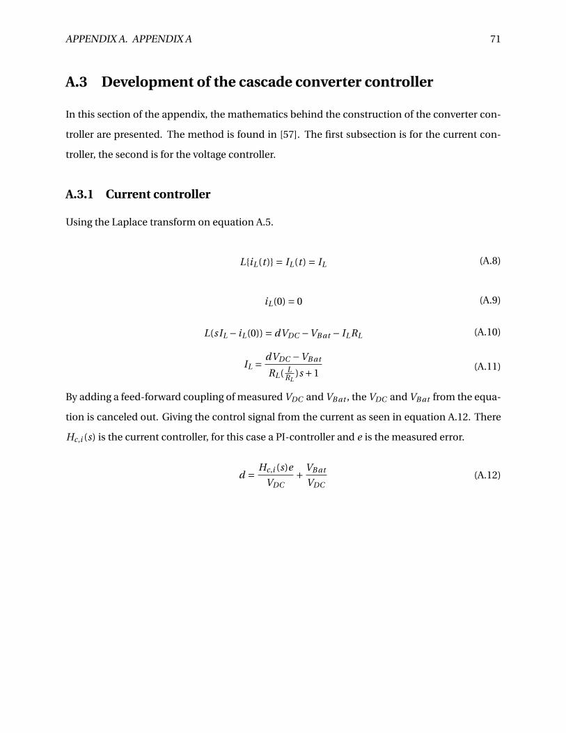
APPENDIX A. APPENDIX A 71
A.3 Development of the cascade converter controller
In this section of the appendix, the mathematics behind the construction of the converter con-
troller are presented. The method is found in [57]. The first subsection is for the current con-
troller, the second is for the voltage controller.
A.3.1 Current controller
Using the Laplace transform on equation A.5.
LiL(t ) = IL(t ) = IL (A.8)
iL(0) = 0 (A.9)
L(sIL − iL(0)) = dVDC −VB at − ILRL (A.10)
IL = dVDC −VB at
RL( LRL
)s +1(A.11)
By adding a feed-forward coupling of measured VDC and VB at , the VDC and VB at from the equa-
tion is canceled out. Giving the control signal from the current as seen in equation A.12. There
Hc,i (s) is the current controller, for this case a PI-controller and e is the measured error.
d = Hc,i (s)e
VDC+ VB at
VDC(A.12)

APPENDIX A. APPENDIX A 72
Figure A.2: Block diagram of the control loop with the feed-forward voltage. Source: [57]
Implanting equation A.12 in A.11, solving for IL and obtain equation A.13.
IL = 1
RL
Hc,i (s)e
( LRL
)s +1(A.13)
The current controller can be tuned with the modulus optimum criterion. For this tuning cri-
terion, the smaller time constants are merged into a single time constant Tsum . The open loop
transfer function can then be written as below , there the first part represent the PI-regulator.
[52]
hol (s) = Kp1+Ti s
Ti sKs
1
1+Tsum ∗ s
1
1+T1s(A.14)
In the equation Tsum = Tsw +Tdel ay , and the controller parameters are:
Ti = T1 (A.15)
Kp = T1
2KsTsum(A.16)
The open loop transfer function for the current controller is:
IL(s) = Kp,i1+Ti ,i s
Ti ,i s
1
1.5m
1
0.44ms
1
1+ 0.361m1.5m s
(A.17)
Results in Kp,i = 0.411 and Ti ,i = 0.241.

APPENDIX A. APPENDIX A 73
A.3.2 Voltage controller
Using the Laplace transform on equation A.4.
LVDC (t ) =VDC (t ) =VDC (A.18)
VDC (0) = 0 (A.19)
Cout (sVDC −VDC (0)) = D IL − VDC
RPL(A.20)
VDC = D IL
Cout s + 1RLP
(A.21)
Figure A.3: Block diagram of the voltage control loop. Source: [57]
For the design of the voltage controller, RLP equals infinity. Then the expression is a integral as
seen in equation A.22.
VDC = D IL
Cout s(A.22)
For the tuning of the voltage controller, symmetrical optimum design criterion was used. Then
the transfer-function with two integrators presented in equation A.23 is the base. [52]
hol (s) = Kp1+Ti s
Ti sKs
1
1+Tsum s
1
T1s(A.23)

APPENDIX A. APPENDIX A 74
Ti and Kp is calculated from the equations:
Ti =βTsum (A.24)
Kp = T1
Ks√βTsum
(A.25)
The time constant Tsum equals 15∗0.33 = 5ms and is calculated from Tsw or the sampling time
of the system Ts . For the tuning β is selected to be four. The transfer function for the voltage
controller is:
VDC (s) = Kp,o1+Ti ,o s
Ti ,o sD
1
1+Tsum s
1
Cout sIL (A.26)
From the equations above, Tio = 0.02 and Kp,o = 1.625. D is the stationary duty ratio (VB at /VDC ).
A.4 Calculations of fuel costs
In this section, the SEC in kJ/kWh is calculated to amount in kg to find the total cost in NOK. The
calculations are based on characteristics of the LNG, information from professor Lars.O Nord at
NTNU and "Natural Gas Conversion Pocketbook" created by IGU. The generator power is mul-
tiplied with the simulation time to get the energy [kWh].
SECk J = (PG1 ∗ t
3600)∗SECG1 (A.27)
The SEC is then multiplied with the heat value of the LNG to get kilograms. (52 MJ/kg) [38]
SECkg = SECk J ∗kg
52000k J(A.28)
The price on LNG is around 4.5 dollar/MMBtu. [21] Btu stands for British thermal unit, where
1M MB tu = 20.3kg LNG and 1$ = 8.1294kr . [1]

APPENDIX A. APPENDIX A 75
4.5$
M MB tu= 1.8
kr
kg(A.29)
The fuel cost can then be calculated for different power and SEC levels with the equation pre-
sented in this section.

B | Appendix B
B.1 The Simulink model
Figure B.1: Simulink model of the AVR and exciter
76

APPENDIX B. APPENDIX B 77
Figure B.2: Simulink model of AC1A in discrete form
B.2 Matlab script for calculation of SEC
Figure B.3: Calculation of SEC with variable speed

APPENDIX B. APPENDIX B 78
Figure B.4: Calculation of SEC with fixed speed
B.3 Actual load scenario
Table B.1: Phases, duration, consumption and MCRPhases Time [s] Consumption [kWh] MCR [kW]
Manoeuvring from the dock 10 6,00 2 160,00Acceleration to march speed 128 165,33 4 650,00
Marching speed 2308 2 660,61 4 150,00Deceleration 130 7,22 200,00
Manoeuvring into the dock 124 74,40 2 160,00Loading and unloading 300 64,58 775,00
Total 3000 2 978,14

C | Appendix C
C.1 Testing of the model
Figure C.1: Power production during 60 seconds at 800 kW load
Figure C.2: Speed of the engine for variable speed during 60 seconds
79

APPENDIX C. APPENDIX C 80
Figure C.3: Power production with KP ×25. during load reduction
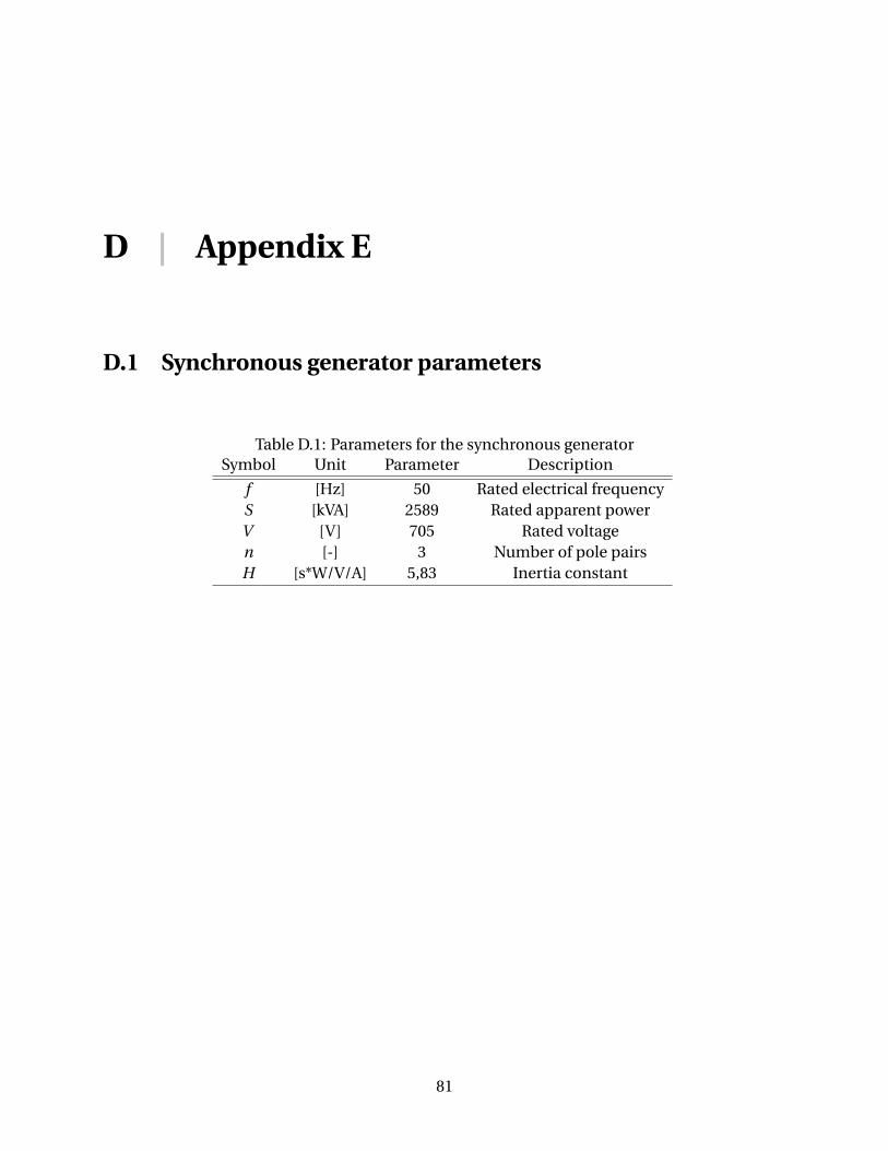
D | Appendix E
D.1 Synchronous generator parameters
Table D.1: Parameters for the synchronous generatorSymbol Unit Parameter Description
f [Hz] 50 Rated electrical frequencyS [kVA] 2589 Rated apparent powerV [V] 705 Rated voltagen [-] 3 Number of pole pairsH [s*W/V/A] 5,83 Inertia constant
81

APPENDIX D. APPENDIX E 82
D.2 Parameter Setting of excitation model AC1A
Table D.2: Parameter settings for AC1A. Terminal voltage transducer: TR = 0,RC = 0.XC = 0Symbol Unit Parameter Description
K A [pu] 200 Regulator output gainTA [s] 0,095 Regulator output time constant
VRM AX [pu] 10 Maximum controller output voltageVRM I N [pu] -10 Minimum controller output voltage
KE [pu] 1 Exciter field proportional constantTE [s] 1,75 Exciter field time constantK f [pu] 0,0374 Damping filter proportional constantT f [s] 0,77 Damping filter time constant
SE [EF D1] [pu] 1,9737 Saturation factor at EF D1
EF D1 [pu] 12,2 Exciter flux at SE [EF D1]SE [EF D2] [pu] 0,2353 Saturation factor at EF D2
EF D2 [pu] 9,3 Exciter flux at SE [EF D2]VAM AX [pu] 14,5 Maximum internal voltageVAM I N [pu] -14,5 Minimum internal voltage
KC [pu] 0.1 Rectifier regulation factorKD [pu] 1.2 Exciter internal reactanceTr [s] 1,75 Voltage sensing and compensation time constant
D.3 Parameters setting of GAST and speed governor
Table D.3: Parameter settings for the GAST and the speed governorSymbol Unit Parameter Description
KS [pu] 25 Speed governor proportional gainTi [s] 1 Speed governor time constant
K f b [pu] 0 Feedback gainT1 [s] 0,05 Controller time constantT2 [s] 0,1 Load limiter time constantT3 [s] 5,0 Temperate limiter time constantKT [s] 5,0 Temperate limiter gain
Vmax [pu] 1,0 Controller maximum outputVmi n [pu] 0,0 Controller minimum output

Bibliography
[1] Valutakurser, 2017. URL http://www.norges-bank.no/statistikk/valutakurser/
valuta/USD. Accessed: 21.05.2018.
[2] Europeancommission, 2017. URL https://ec.europa.eu/clima/policies/
transport/shipping_en. Accessed: 07.04.2018.
[3] ABB, Onboard DC-grid, 2018. URL https://new.abb.com/marine/marine/
systems-and-solutions/power-generation-and-distribution/onboard-dc-grid.
Accessed: 24.05.2018.
[4] Ampere, 2018. URL http://viewer.zmags.com/publication/061eea2c#/061eea2c/6.
Accessed: 24.05.2018.
[5] How to measure state of charge, 2018. URL http://batteryuniversity.com/learn/
article/how_to_measure_state_of_charge. Accessed: 16.05.2018.
[6] Configuration of the battery, 2018. URL http://batteryuniversity.com/learn/
article/serial_and_parallel_battery_configurations. Accessed: 24.04.2018.
[7] Battery performance, 2018. URL http://www.mpoweruk.com/performance.htm. Ac-
cessed: 24.04.2018.
[8] Charging of the lithium battery, 2018. URL http://batteryuniversity.com/learn/
article/charging_lithium_ion_batteries. Accessed: 25.04.2018.
[9] Effects of Harmonics, 2018. URL http://www.ecmweb.com/power-quality/
effects-harmonics-power-systems. Accessed: 20.05.2018.
83

BIBLIOGRAPHY 84
[10] Battery specifications, 2018. URL http://web.mit.edu/evt/summary_battery_
specifications.pdf. Accessed: 25.04.2018.
[11] Frequency switching regulator, 2018. URL www.digikey.com/en/articles/techzone/
2015/feb/design-trade-offs-when-selecting-a-high-frequency-switching-regulator.
Accessed: 05.03.2018.
[12] MathWorks, AC1A Excitation System, 2018. URL https://se.mathworks.com/help/
physmod/sps/powersys/ref/ac1aexcitationsystem.html. Accessed: 30.04.2018.
[13] MathWorks, Battery model, 2018. URL https://se.mathworks.com/help/physmod/
elec/ref/battery.html. Accessed: 02.05.2018.
[14] MathWorks, Synchronous Machine Field Circuit (pu), 2018. URL https://se.mathworks.
com/help/physmod/sps/ref/synchronousmachinefieldcircuitpu.html. Accessed:
30.04.2018.
[15] MathWorks, Mean, 2018. URL https://se.mathworks.com/help/physmod/sps/
powersys/ref/mean.html. Accessed: 06.05.2018.
[16] MathWorks, Rectifier, 2018. URL https://se.mathworks.com/help/physmod/sps/ref/
rectifier.html. Accessed: 06.05.2018.
[17] MathWorks, Synchronous Machine Salient Pole (Standard),
2018. URL https://se.mathworks.com/help/physmod/sps/ref/
synchronousmachinesalientpolestandard.html. Accessed: 30.04.2018.
[18] Matlab home page, 2018. URL https://se.mathworks.com/products/matlab.html.
Accessed: 05.03.2018.
[19] Non regenerative vs regenerative, 2018. URL www.quantum-controls.co.uk/faq/
drives/whats-the-difference-between-a-non-regenerative-dc-drive-and-a-regenerative-dc-drive/.
Accessed: 26.04.2018.
[20] Simscape power systems, 2018. URL https://se.mathworks.com/products/simpower.
html. Accessed: 07.04.2018.

BIBLIOGRAPHY 85
[21] Spot price for LNG, 2018. URL https://www.icis.com/press-releases/
lng-markets-analysis-spot-lng-prices-hold-steady-in-balanced-market/.
Accessed: 20.04.2018.
[22] Newpaper of torghatten, 2018. URL https://sysla.no/maritim/
vard-skal-bygge-to-nye-lng-ferger-for-torghatten/. Accessed: 06.05.2018.
[23] Bijan Zahedi, Lars Einar Norum. Voltage regulation and power sharing control in ship LVDC
power distribution systems. Power Electronics and Applications, 15:1–8, 2013.
[24] Bijan Zahedi, Lars Einar Norum. An Isolated Bidirectional Converter Modeling for Hybrid
Electric Ship Simulations. Power Electronics and Applications, 15:1–6, 2013.
[25] Bijan Zahedi, Lars Einar Norum. Voltage regulation and power sharing control in ship LVDC
power distribution systems. Power Electronics and Applications, 15:1–8, 2013.
[26] DNV GL. RULES FOR CLASSIFICATION, General regulations. Rules for classification, DNV
GL, 2017.
[27] DNV GL. Part 4 Systems and components, Chapter 8 Electrical installations. Rules for
classification, DNV GL, 2018.
[28] DNV GL. Part 6 Additional class notations, Chapter 2 Propulsion, power generation and
auxiliary systems. Rules for classification, DNV GL, 2018.
[29] DNV GL. Part 4 Systems and components, Chapter 9 Control and monitoring systems.
Technical report, DNV GL, 2018.
[30] DR. Pierre C.Sames, MR Niels B. Clausen,Mr. Mads Lyder Andersen. Costs and Benefits of
LNG as Ship Fuel for Container Vessels. MAN Diesel Turbo, 1:1–18, 2011.
[31] Eleftherios K. Dedes, Dominic A. Hudson, Stephen R. Turnock. Assessing the potential of
hybrid energy technology to reduce exhaust emissions from global shipping. Energy Policy,
40:204–218, 2011.
[32] Georgios Karmiris, Tomas Tengner. PEAK SHAVING CONTROL METHOD FOR ENERGY
STORAGE. ABB AB, Corporate Research Center, 1:1–6, 2012.

BIBLIOGRAPHY 86
[33] Giovanni Petrecca. Energy Conversion and Management. Springer, Cham, Energy Conver-
sion and Management, 1nd edition, 2014.
[34] Guerrero, Josep M.; Vásquez, Juan V.; Teodorescu, Remus. Hierarchical Control of Droop-
Controlled DC and AC Microgrids - A General Approach Towards Standardization. IEEE
Industrial Electronics Society, 1:4341–4346, 2009.
[35] IEEE. IEEE Recommended Practice for Excitation System Models for Power System Stability
Studies. Standard, IEEE Power Engineering Society, 2006 April.
[36] IEEE and IEEE PES. Dynamic Models for Turbine-Governors in Power System Studies .
Technical report, IEEE, 2013 Jan.
[37] Il-Yop Chung, Wenxin Liu, Mike Andrus, Karl Schoder, Siyu Leng, David A. Cartes, and Mis-
cha Steurer. Integration of a Bi-directional DC-DC Converter Model into a Large-scale
System Simulation of a Shipboard MVDC Power System. IEEE Electric Ship Technologies
Symposium, 1:318–325, 2009.
[38] International Gas Union IGU. Natural Gas Conversion Pocketbook. Manual, IGU, 2012.
[39] Juming Lai. Parameter Estimation of Exitation Systems. Master thesis, Graduate Faculty of
North Carolina State University, 2007.
[40] Junhong Zhang. Bidirectional DC-DC Power Converter Design Optimization, Modeling
and Control. Doctor thesis, Virginia Polytechnic Institute and State University, 2008.
[41] Junhong Zhang. Bidirectional DC-DC Power Converter Design Optimization, Modeling
and Control. Doctor Thesis, Virginia Polytechnic Institute and State University, 2008-
January.
[42] Kyunghwa Kim, Kido Park, Jongwoo Ahn, Gilltae Roh and Kanwoo Chun. A Study on Appli-
cability of Battery Energy Storage System (BESS) for Electric Propulsion Ships. Transporta-
tion Electrification Asia-Pacific, 5:203–207, 2016.
[43] Mahat, Pukar; Chen, Zhe; Bak-Jensen, Birgitte. Gas turbine control for islanding operation
of distribution systems. Energy Society General Meeting 2009, 15:1–7, 2009.

BIBLIOGRAPHY 87
[44] Mahendra Chandra Joshi. Modeling and Control of Bidirectional DC DC Converter Fed
PMDC Motor. Master thesis, Institute of Technology Rourkela Rourkelay, 2013 May.
[45] Mahesh Swamy, Steven Schifko. An Improved Active Front End NonRegenerative Rectifier
System Employing a Five-Limb Inductor. Electric Machines Drives Conference (IEMDC),
2013 IEEE International, 15:1241–1248, 2013.
[46] Martin Skaar Vadset. Dynamic Models for Turbine-Governors in Power System Studies.
Technical report, NTNU, 2017 Des.
[47] Mukund R. Patel. SHIPBOARD ELECTRICAL POWER SYSTEMS. CRC Press, Taylor Francis
Group, Converters, Applications, and Design, 3nd edition, 2003.
[48] Ned Mohan, Tore M. Undeland, William P. Robbins. Power Electronics. John Wiley Sons,
INC, Converters, Applications, and Design, 3nd edition, 2003.
[49] Ole Christian Nebb. Use of Energy Storage in a LVDC Distribution Network for Ships. Mas-
ter thesis, Norwegian University of Science and Technology, 2012 June.
[50] Ole Christian Nebb, Bijan Zahedi, John Olav Lindtjorn, Lars Norum. Increased fuel effi-
ciency in ship LVDC power distribution systems. Vehicle Power and Propulsion, 93:564–568,
2012.
[51] Rolls-Royce. Bergen engine type C26:33 Gas. Project guide, Rolls-Royce, 2018.
[52] Roy Nilsen. TET4120, Electric Drives. NTNU, Lecture Notes, 1nd edition, 2018.
[53] Roy Nilsen, Ingve Sorfonn. Hybrid Power Generation Systems. Power Electronics and Ap-
plications, 13:1–9, 2009.
[54] S.A. Talib, S.M. Bashi, N.F. Mailah. Simulation and analysis of power converter harmonics.
Student Conference on Research and Development, 1:213–216, 2009.
[55] Sven De Breucker. IMPACT OF DC-DC CONVERTERS ON LI-ION BATTERIES. Doctor the-
sis, Katholieke Universiteit Leuven, 2012 December.
BIBLIOGRAPHY 88
[56] Torstein Ingebrigtsen Bø. Scenario- and Optimization-Based Control of Marine Electric
Power Systems. Doctor thesis, NTNU, 2016 March.
[57] Tron Hansen Syverud. Modeling and Control of a DC-grid Hybrid Power System with Bat-
tery and Variable Speed Diesel Generators. Master Thesis, NTNU, 2016-June.