Örebro University

Örebro University School of Business

Masters in Applied Statistics

Sune karlsson

Farrukh Javed

JUNE, 2016

Modeling and Forecasting Unemployment Rate

In Sweden using various Econometric Measures

Meron Desaling (86/01/30)

Acknowledgments First, and foremost, I would like to thank the almighty God for giving me the opportunity

to pursue my graduate study at Department of Applied Statistics, Orebro University.

I owe the deepest gratitude to Prof.Sune karlsson, my thesis advisor for his valuable and

constructive comments and encouragements throughout my study.

My deepest thanks go to my family, who have supported me all the way to fulfill my

dream.

TABLE OF CONTENTS ACRONYMS………………………………………………………………...................……………………..I ABSTRACT……………………………………………………...................………………………………...II CHAPTER1:INTRODUCTION...................................................................................................................1 1.1Introduction ………………………………………………………………………..………......1 1.2 Objectives of the Study.............................................................................................................................4

CHAPTER 2: LITERATURE REVIEW.......................................................................................................5

2.1 Review of Literature…...................…………………………...………………………………….............5

CHAPTER 3 : DATA AND METHODOLOGY...........................................................................…..........7 3.1 Data...................................……………………………….…………………………………........................7

3.2 Methodology…………...………………………….……………………………........................................7

3.3 Stationary Test........................................................................................................................................8

3.4 Lag length selection................................................................................................................................11

3.5 Time series models………………………………………………………………...............................11

3.5.1 Univariate time series model .....................................................................................................12

3.5.1.1 Seasonal Autoregressive Integrated Moving Average Model (SARIMA).................12

3.5.1.2 Self-Exciting Threshold Autoregressive (SETAR) Model............................................14

3.5.2.Multivariate time series model ....................................................................................................17

3.5.2.1. Vector Autoregressive Model ..............................................................................................17

3.6 Model checking.……………………………………………………………………...............................21

3.6.1 Residual Analysis..........................................................................................................................22 3.6.1.1 Residual autocorrelation test.................................................................................................22

3.6.1.2 Residuals normality test.....................................................................................................24

3.7 Forecasting .............................................................................................................................................. 26

3.7.1 Out sample forecasting method..................................................................................................27

3.7.2 Forecasting Accuracy.…………………………………………………..........…………............27

CHAPTER 4: RESULT AND DISCUSSION………………………………………………..................30

4.1 Descriptive Analysis………………………………………………………………................................30

4.2 Stationary test Analysis.…………………………………………………………….............................30

4.3 Modeling Seasonal Autoregressive integrated moving average model.....……………..................35

4.4 Modeling Self Exciting Threshold Autoregressive Model…………….........................................47

4.5 Modeling of Vector Autoregressive Model....................................................................................40

4.6 Comparison of Models Forecasting Performance............................................................................44

4.7 Forecasting Result..................................................................................................................................45

CHAPTER 5: CONCLUSION AND RECOMMENDATION………………………………......47

5.1 Conclusions.….............……………………………………………………………………………….....47 5.2 Recommendations……………………………………….............……………………………………...47

REFERENCES…………………………………………………………………………………...................48 ANNEX1: STATA and R outputs.................………………………………………………...........….......50

Table A1: SARIMA Models Comparison …………….........……………………………………….......50

Table A2: Result for TAR model...……………………….……………...........……………….................51

Table A3: VAR order selection test using lag four, six and seven..................……………….............52

Table A4: Pair-wise Granger-causality tests……….….........……………………………………...........53

ACRONYMS

VAR Vector Autoregressive

SETAR Self Exciting threshold autoregressive

SARIMA Seasonal autoregressive integrated moving average

AIC Akaike Information Criteria

BIC Schwartz and Bayes Information Criterion

HQ Hannan-Quin

OECD Organization for Economic Cooperation and Development

ADF Augmented Dickey-Fuller

PP Phillips -Perron

LM Lagrange multiplier

ACF Autocorrelation Function

PACF Partial Autocorrelation Function

RMSE Root mean square error

MAE Mean absolute error

MAPE Mean Absolute percentage error

DM Diebold-Mariano

I

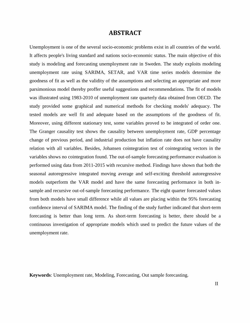
ABSTRACT

Unemployment is one of the several socio-economic problems exist in all countries of the world.

It affects people's living standard and nations socio-economic status. The main objective of this

study is modeling and forecasting unemployment rate in Sweden. The study exploits modeling

unemployment rate using SARIMA, SETAR, and VAR time series models determine the

goodness of fit as well as the validity of the assumptions and selecting an appropriate and more

parsimonious model thereby proffer useful suggestions and recommendations. The fit of models

was illustrated using 1983-2010 of unemployment rate quarterly data obtained from OECD. The

study provided some graphical and numerical methods for checking models' adequacy. The

tested models are well fit and adequate based on the assumptions of the goodness of fit.

Moreover, using different stationary test, some variables proved to be integrated of order one.

The Granger causality test shows the causality between unemployment rate, GDP percentage

change of previous period, and industrial production but inflation rate does not have causality

relation with all variables. Besides, Johansen cointegration test of cointegrating vectors in the

variables shows no cointegration found. The out-of-sample forecasting performance evaluation is

performed using data from 2011-2015 with recursive method. Findings have shown that both the

seasonal autoregressive integrated moving average and self-exciting threshold autoregressive

models outperform the VAR model and have the same forecasting performance in both in-

sample and recursive out-of-sample forecasting performance. The eight quarter forecasted values

from both models have small difference while all values are placing within the 95% forecasting

confidence interval of SARIMA model. The finding of the study further indicated that short-term

forecasting is better than long term. As short-term forecasting is better, there should be a

continuous investigation of appropriate models which used to predict the future values of the

unemployment rate.

Keywords: Unemployment rate, Modeling, Forecasting, Out sample forecasting.

II

1

CHAPTER ONE

1.1 INTRODUCTION

Unemployment is one of the several socio-economic problems exist in all countries of the world.

It affects people's living standard and nations' socio-economic status.

The main reason for increasing unemployment rate is the deficiency of demand in the economy

to maintain full employment. When there is less demand, companies need less labor input,

leading them to cut hours of work or laying people off. Though unemployment is mainly caused

by a fundamental shift in an economy, its frictional, structural, and cyclical behavior also

contributes to its existence.

Frictional unemployment is unemployment which exists in any economy due to the inevitable

time delays in finding new employment in a free market. Structural unemployment occurs for

many reasons, such as people may lack the needed job skills or they may live far from locations

where jobs are available but unable to move there. Besides, sometimes people may be unwilling

to work because existing wage levels are too low. Consequently, while jobs are available, there is

a serious mismatch between what companies need and what workers can offer. In general,

structural unemployment is increased by external factors like technology, competition, and

government policy. Moreover, cyclical unemployment is a factor for unemployment related with

the cyclical trend of economic indicators which exist in a business cycle. Cyclical unemployment

declines at business cycles increased in output since the economy gets maximized. On the other

hand, when the economy measured by the gross domestic product (GDP) declines, the business

cycle becomes lower and cyclical unemployment gets a rise. Economists define cyclical

unemployment as the result of companies have a lack of demand for labor to hire individuals,

who are looking for work. It is logical when the economy gets down the lack of employer

demand will exist.

At any time and economy status of a country, there is some level of unemployment. Due to its

fractional and structural behavior, unemployment is positive rather zero. The natural level of

unemployment is the unemployment rate when an economy is operating at full capacity. The

2

quantity of labor supplied equals the quantity of labor demanded at the natural level. Mainly, the

natural rate of unemployment is determined by an economy's production possibilities and

economic institutions. Besides, it is a rate at which there is no tendency for inflation to accelerate

or decelerate. Consequently, when an economy is at the natural rate inflation is constant. For this

reason, the natural rate of unemployment is sometimes called constant inflation rate of

unemployment.

THE SOCIO ECONOMIC EFFECT OF UNEMPLOYMENT

1). The social effects of unemployment

Unemployment affects both the individuals and their families. In the long run, it also affects the

society. Unemployment causes for a mental health problem and on the physical well-being of

individuals. Hammarstrom and Janlert (1997), stated that those who are unemployed expected to

experience different emotions such as sadness, hopelessness, humiliation, worry, and pain.

Besides, according to Britt, 1994; Weich and Lewis, 1998; Reynolds, 2000, report different

crimes prevail in a society when there is a high unemployed group in the population. Health

problems, drug abuse, and similar problems are highly associated with unemployment.

2). Unemployment affects economy

Economists describe unemployment is a lagging indicator of the economy, as the economy

usually recovers before the unemployment rate starts to rise again. However, unemployment

causes a sort of wave effect across the economy. As people losing their job, they do not pay state

and federal income taxes, and additional sales tax revenue. Instead as a laid off worker, they

could immediately cut back to their unnecessary cost due to less disposable income and this

cause for less money to be spent in the economy, driving to more people to miss their jobs.

Consequently, the process recycles unless it is broken by developing a policy and plan.

In general, the rising of unemployment rate highly affects different economy factors such as

personal income, cost of health, health care quality, leaving standard and poverty. All those

affect the entire systems of the economy as well as the society.

3

Trend of Sweden unemployment rate

In Sweden, the unemployment rate is defined as the number of unemployed individuals

calculated as a percentage of individuals in the labor force, which includes both the employed

and unemployed.

The average unemployment rate in Sweden from 1980 until 2016 is 5.88 percent. During this

period, the highest was 10.50 percent reported in June 1997 and the lowest was 1.30 percent

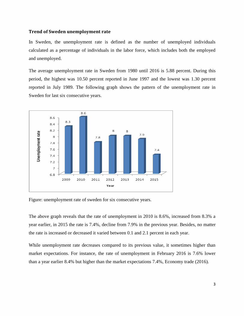
reported in July 1989. The following graph shows the pattern of the unemployment rate in

Sweden for last six consecutive years.

Figure: unemployment rate of sweden for six consecutive years.

The above graph reveals that the rate of unemployment in 2010 is 8.6%, increased from 8.3% a

year earlier, in 2015 the rate is 7.4%, decline from 7.9% in the previous year. Besides, no matter

the rate is increased or decreased it varied between 0.1 and 2.1 percent in each year.

While unemployment rate decreases compared to its previous value, it sometimes higher than

market expectations. For instance, the rate of unemployment in February 2016 is 7.6% lower

than a year earlier 8.4% but higher than the market expectations 7.4%, Economy trade (2016).

4

Since unemployment is closely related to the state of the economy predicting the unemployment

rate has value to various economic decisions. It is used for both monetary policy makers to

serves as an indicator of the stance of the macroeconomic in general and carries information

regarding inflationary pressure as well as for fiscal policy makers related to the government

expenditure and income due to its relationship with, for instance, income taxes and

unemployment benefits. Therefore, signals of future unemployment rates are necessary for

policy and decision makers to plan and strategize before time. Consequently, this study focuses

on modeling and forecasting the rate of unemployment in Sweden.

1.2 General objective of the study

The main objective of the study is to modeling and forecasting the unemployment in Sweden. In

this case, the study fit univariate and multivariate time series models for the unemployment rate

and other macroeconomic variables which can be used to achieve the objective.

Specific objectives

Modeling the linear and asymmetry behavior of unemployment rate

Comparing the forecasting performance of different models

Forecasting unemployment rate in different horizons

5

CHAPTER TWO

2.1 LITERATURE REVIEW

Modeling and forecasting of macroeconomic variables used to address different issues related to

the economic state of the countries. Researchers have used various time series models for

modeling and forecasting of macroeconomic variables. The unemployment rate is one of the

macroeconomic variables, modeling, and forecasting of it have a great importance for many

economic decisions. Different models have been used to modeling and forecasting as well as to

compare the forecasting performance of models for the unemployment rate of several countries.

Like any other economic variables modeling of unemployment rates have been analyzed by

building econometric models, often related to stationary time series, seasonality and trend

analysis, and exponential smoothening to the simple OLS technique including autoregressive

integrated moving average(ARIMA) models.

The suitability of the ARIMA models for forecasting macroeconomic variables is studied by

various researchers; Power and Gasser (2012) investigate that an ARIMA (1,1,0) model has

better forecasting performance for unemployment rates in Canada. Besides, an ARIMA (1,2,1)

model is suitable for forecasting the unemployment rate in Nigeria, as reported by Etuk et

al.(2012).

VAR model is one of the most useful time series models to describe the dynamic behavior of

macroeconomic variables and to forecast. Clements and Hendry (2003) stated that the accuracy

of forecasts based on VAR models can be measured using the trace of the mean-squared

forecasts error matrix or generalized forecasts error second moment. Robinson (1998)

demonstrated better accuracy for predictions of some macroeconomic variables based on VAR

models compared to other models, like transfer functions. Finally, Lack (2006) found that

combined forecasts based on VAR models are a good strategy for improving predictions’

accuracy.

Kishor and Koenig (2012) made predictions for macroeconomic variables like unemployment

rate using VAR models and taking into account that data are subject to revisions.

6

The unemployment rate reacts in a different way to contraction and expansion phases of the

general business cycle. It faster moves upward in a general business slowdown and slowly

downward in speedup phases. The asymmetric nature of the business cycle can be considered the

main source of nonlinearity in the unemployment time series. The classical linear models are not

able to describe these dynamic asymmetries and nonlinear time series models would be required.

However, the asymmetric behavior of unemployment rate can be modelled using nonlinear time

series model. Skalin and Terasvirta (1998) propose STAR model in order to capture the

asymmetry property of unemployment rate. They assume that unemployment rate is a stationary

nonlinear variable.

Peel and Speight (2000), examine whether a Self-Exciting Threshold Autoregressive (SETAR|)

models are able to provide better out-of-sample forecasts compared to an Autoregressive model

using Uk unemployment sample data from February 1971 to September 1991. The result shows

that SETAR models have better forecasting performance relative to AR models in terms of

RMSE. Koop and Potter (1999) use threshold autoregressive (TAR) for modeling and

forecasting the US monthly unemployment rate. Rothman (1998) compares out-of-sample

forecasting accuracy six nonlinear models, and Parker and Rothman (1998) model the quarterly

adjusted rate with AR(2) model. Proietti (2001) used seven forecasting models (linear and non-

linear) to examine the out-of-sample forecasting for the US monthly unemployment rate. The

result reveals that linear models have better forecasting performance than nonlinear models.

Besides, Jones(1999), Gil-Alana(2001) reported, in different research papers, the modeling and

forecasting of the unemployment rate in the UK. Johns (1999) examines the forecasting

comparison between AR(4), AR(4)-GARCH(1,1), SETAR(3,4,4), Neural network and Naïve

forecast of UK monthly unemployment rate with the sample data from January 1960 to August

1996. The result reveals that SETAR model is better than the others for short period forecasts,

while non-linearity was present in the data.

Moreover, Gil-Alana (2001) used a Bloomfield exponential spectral model for modeling UK

unemployment rate, as an alternative to the ARMA models. The results reveal that this model is

reasonable to model UK unemployment rate.

7

CHAPTER THREE

3. DATA AND METHODOLOGY 3.1. Data:

This study used Sweden unemployment rate quarterly data from the first quarter of 1983 to the

fourth quarter of 2015, with a total number of 132 observations collected from OECD. The first

112 observations are used to model estimation and the rest 20 observations to evaluate model

forecasting performance.

Variables in the study

Since the study uses both univariate and multivariate time series models to model the

unemployment rate in Sweden, the study considers some additional economic variables which

have a direct or indirect relation with unemployment. According to economic theory, there is a

direct relationship between gross domestic product and unemployment rate. The GDP get lower

when unemployment rate becomes above its natural rate and vice-versa. There is also a

relationship between unemployment rate and industrial production, potential output measures the

productive capacity of the economy when unemployment is at its natural rate. In most cases the

produced output is proportional to the level of the inputs (capital and labor). Thus, an increasing

unemployment above its natural rate is related to the falling of output below its potential and

vice-versa. Moreover, there is an indirect relation between the rate of unemployment and the rate

of inflation. Consequently, in addition to model unemployment rate alone, the study also model

it together with GDP percentage change of previous period, industrial production, and inflation

rate.

3.2. METHODOLOGY

Time series can be defined as any series of measurements taken at different times, can be divided

into univariate and multivariate time series. Univariate time series analysis uses one series.

However, the multivariate time series analysis involves more than one series data sets used when

one wants to model and explain the effect and relation among time series variables.

8

3.3. TESTING STATIONARY

Unit root test without structural break

Before fitting a particular model to time series data, the stationarity of a series must be checked.

Stationarity occurs in a time series when the mean and autocovariance of the series remains

constant over the time series. It means that the joint statistical distribution of any collection of

the time series variates never depends on time. Therefore, the stochastic process yt is said to be

stationary if:

i. ,)( tyE constant for all value of t .......................................(1)

ii. The T

j

T

jttjjtt yyEyyCov ))((),( for all t and j=0,1,2, ...................(2)

Equation (1) means that yt have the same finite mean μ through the process and (2) requires that

the autocovariance of the process do not depend on t but just on the time period j, the two

vectors yt and yt-j are apart. Therefore, a process is stationary if its first and second moments are

time invariant.

Usually, differencing may be needed to achieve stationarity. Several methods have been

developed to test the stationarity of a series. The most common ones are Augmented Dickey-

Fuller (ADF) test due to Dickey and Fuller (1979, 1981), and the Phillip-Perron (PP) due to

Phillips (1987) and Phillips and Perron (1988). The following discussion outlines the basics

features of unit root tests (Hamilton, 1994).

Consider a simple AR (1) process:

ttt yy 1 ..............................................(3)

Where yt is the variable of interest, t is time index, is parameter to be estimated, and t is

assumed to be a white noise. If ,1 yt is a non stationary series and the variance of yt

increases with time and approaches infinity. If ,1 yt is a stationary series. Thus, the

hypothesis of (trend) stationarity can be evaluated by testing whether the absolute value of ρ is

strictly less than one. The test hypothesis is:

9

0H : The series is not stationary (ρ=1)

:1H The series is stationary (ρ<1)

3.3.1. Augmented Dickey-Fuller (ADF) Test

The standard Dickey-Fuller test is conducted by estimating equation (3) after subtracting 1ty

from both side of the equation

ttt yy 1 .......................(4)

where ᾳ=ρ-1 and 1 ttt yyy . The null and alternative hypothesis may be written as,

0:0 H

0:0 H ........................................(5)

and evaluated using the conventional t-ratio for ᾳ:

))(/(

set ...................................(6)

Where

is the estimate of , and se(

) is the coefficient standard error.

Under the null hypothesis of the unit root test the DF test statistics does not follow the

conventional student t-distribution instead asymptotic t-distribution.

The simple Dickey-Fuller unit root test described above is valid only when the series is an AR(1)

process. If the series is correlated at higher order lags, the assumption of white noise

disturbances ԑt is violated. The Augmented Dickey-Fuller (ADF) test constructs a parametric

correction for higher-order correlation by assuming that the series follows an AR(p) process and

adding lagged difference terms of the dependent variable y to the right-hand side of the test

regression:

tptptttt Uyyyyy ...22111 ..............................(7)

This augmented specification is then used to test (5) using the t-ratio (6). An important result

obtained by Fuller is that the asymptotic distribution of the t-ratio for ᾳ is independent of the

number of lagged first difference included in the ADF regression. Moreover, while the

10

assumption that ty follows an autoregressive (AR) process may seem restrictive, said and Dickey

(1984) demonstrate that the ADF test is asymptotically valid in the presence of a moving average

(MA) component, provided that sufficient lagged difference terms are included in the test

regression.

3.3.2. The Phillips -Perron (PP) Test

Phillips and Perron (1988) proposes an alternative (nonparametric) method of controlling for

serial correlation when testing for a unit root. The PP method estimates the non-augmented DF

test equation (5), and modifies the t-ratio of the ᾳ coefficient so that serial correlation does not

affect the asymptotic distribution of the test statistics. The PP test is based on the statistic:

sf

sefT

ftt

2/1

0

002/1

0

0

2

)(

..............................(8)

where

is the estimate, t is the t-ratio of ᾳ, se(

) is coefficient standard error and s is the

standard error of the test regression. In addition, 0 is a consistent estimate of the error variance

in (5) (calculated as (T-K)s2/T) calculated, where k is the number of regressors). The remaining

term, f0, is an estimator of the residual spectrum at frequency zero.

Unit root test with structural break

3.3.3 Zivot and Andrews Test

Zivot and Andrews endogenous structural break test is a sequential test which uses the full

sample and a different dummy variable for each possible break date. The break date is selected

where the t-statistics of a unit root ADF test is at a minimum (most negative). Consequently, a

break date will be chosen when the evidence does not support the null hypothesis of a unit root.

Zivot and Andrews perform a unit root test with three conditions such as a structural break in the

level of the series; a one-time change in the slope of the trend, and a structural break in the level

and slope of the trend function of the series. Therefore, to test for the null of a unit root against

the alternative of a stationary structural break, Zivot and Andrews (1992), use the following

equations corresponding to the above three conditions.

11

tt

k

j

jttt ydDUtycy

1

1

1 (condition one)

tt

k

j

jttt ydDTtycy

1

1

1 (condition two)

tt

k

j

jtttt ydDTDUtycy

1

1

1 (condition three)

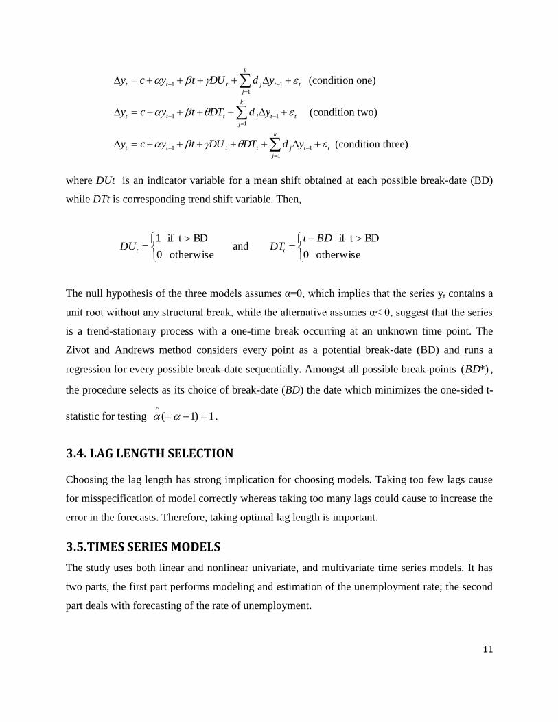
where DUt is an indicator variable for a mean shift obtained at each possible break-date (BD)

while DTt is corresponding trend shift variable. Then,

otherwise 0

BD tif 1tDU and

otherwise 0

BD tif BDtDTt

The null hypothesis of the three models assumes α=0, which implies that the series yt contains a

unit root without any structural break, while the alternative assumes α< 0, suggest that the series

is a trend-stationary process with a one-time break occurring at an unknown time point. The

Zivot and Andrews method considers every point as a potential break-date (BD) and runs a

regression for every possible break-date sequentially. Amongst all possible break-points *)(BD ,

the procedure selects as its choice of break-date (BD) the date which minimizes the one-sided t-

statistic for testing 1)1(

.

3.4. LAG LENGTH SELECTION

Choosing the lag length has strong implication for choosing models. Taking too few lags cause

for misspecification of model correctly whereas taking too many lags could cause to increase the

error in the forecasts. Therefore, taking optimal lag length is important.

3.5.TIMES SERIES MODELS

The study uses both linear and nonlinear univariate, and multivariate time series models. It has

two parts, the first part performs modeling and estimation of the unemployment rate; the second

part deals with forecasting of the rate of unemployment.

12

3.5.1. Univariate Time Series Models 3.5.1.1 Seasonal Autoregressive Integrated Moving Average Model (SARIMA)

For unemployment rate time series, a seasonality might need to consider in ARIMA model. This

process is known as a seasonal process and it drives ARIMA into SARIMA process. Seasonal

Autoregressive Integrated Moving Average (SARIMA) model is a generalized form of ARIMA

model which accounts for both seasonal and non-seasonal characterized data. Similar to the

ARIMA model, the forecasting values are assumed to be a linear combination of past values and

past errors. The SARIMA model also sometimes referred to as the Multiplicative Seasonal

Autoregressive Integrated Moving Average model, is denoted as ARIMA(p,d,q) (P,D,Q)S. The

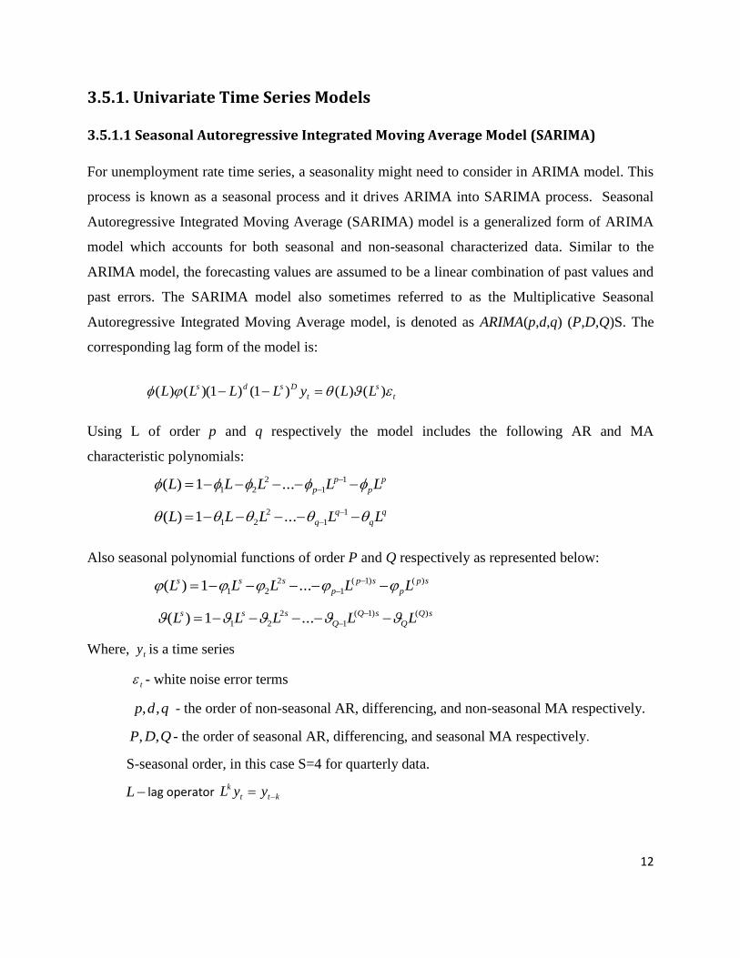
corresponding lag form of the model is:

t

s

t

Dsds LLyLLLL )()()1()1)(()(

Using L of order p and q respectively the model includes the following AR and MA

characteristic polynomials:

p

p

p

p LLLLL

1

1

2

21 ...1)(

q

q

q

q LLLLL

1

1

2

21 ...1)(

Also seasonal polynomial functions of order P and Q respectively as represented below:

sp

p

sp

p

sss LLLLL )()1(

1

2

21 ...1)(

sQ

Q

sQ

Q

sss LLLLL )()1(

1

2

21 ...1)(

Where, ty is a time series

t - white noise error terms

qdp ,, - the order of non-seasonal AR, differencing, and non-seasonal MA respectively.

QDP ,, - the order of seasonal AR, differencing, and seasonal MA respectively.

S-seasonal order, in this case S=4 for quarterly data.

L lag operator ktt

k yyL

13

HEGY test of Seasonality

The first procedure towards designing of SARIMA model is to examine whether the series

satisfy the stationarity condition. This study used Hylleberg Engle-Granger-Yoo (HEGY) test

suggested by Hylleberg et al. (1990) to test for the presence of seasonal unit root in the

observable series. HEGY test is a test for seasonal and non-seasonal unit root in a time series. A

time series 𝑦𝑡 is considered as an integrated seasonal process if it has a seasonal unit root as well

as a peak at any seasonal frequency in its spectrum other than the zero frequency. The test is

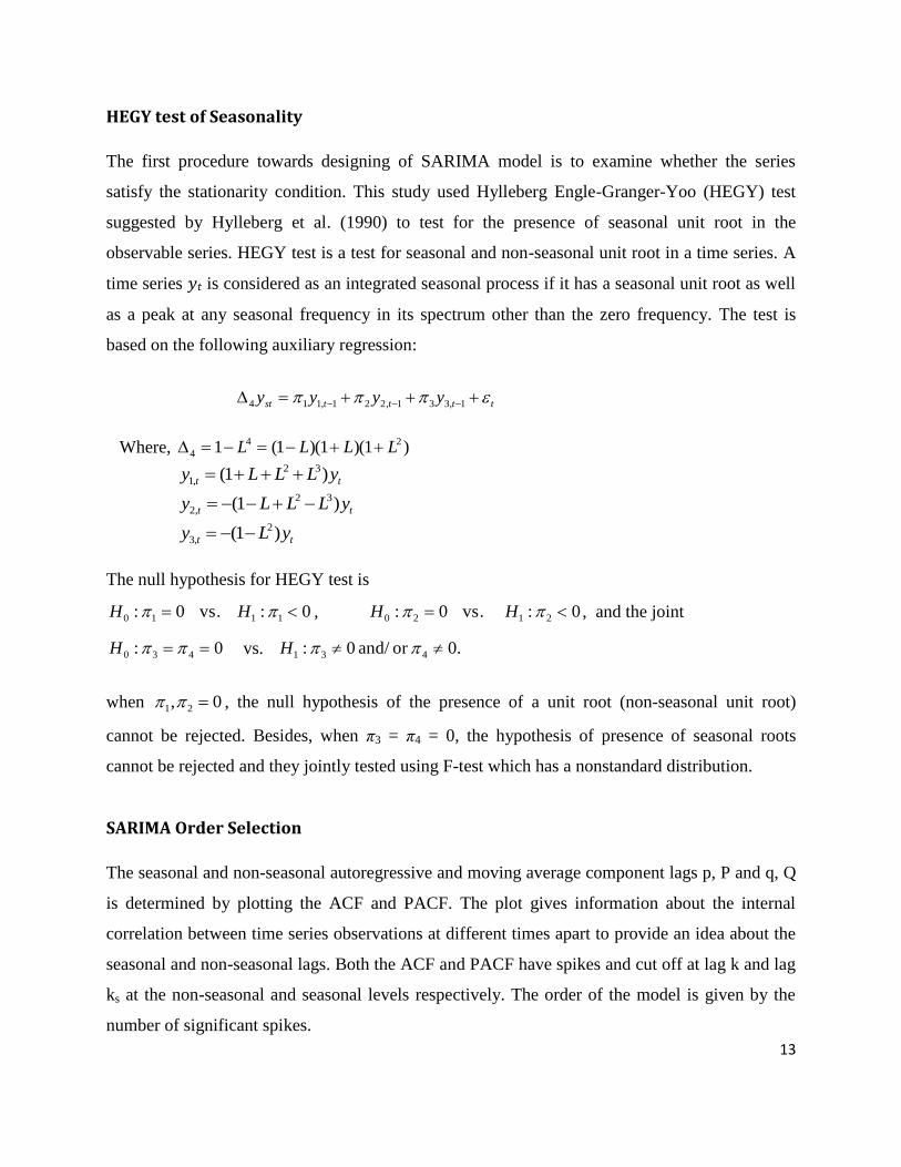
based on the following auxiliary regression:

ttttst yyyy 1,331,221,114

Where, )1)(1)(1(1 24

4 LLLL

tt yLLLy )1( 32

,1

tt yLLLy )1( 32

,2

tt yLy )1( 2

,3

The null hypothesis for HEGY test is

0: vs.0: 1110 HH , 0: vs.0: 2120 HH , and the joint

0: 430 H vs. .0or and/ 0: 431 H

when 0, 21 , the null hypothesis of the presence of a unit root (non-seasonal unit root)

cannot be rejected. Besides, when π3 = π4 = 0, the hypothesis of presence of seasonal roots

cannot be rejected and they jointly tested using F-test which has a nonstandard distribution.

SARIMA Order Selection

The seasonal and non-seasonal autoregressive and moving average component lags p, P and q, Q

is determined by plotting the ACF and PACF. The plot gives information about the internal

correlation between time series observations at different times apart to provide an idea about the

seasonal and non-seasonal lags. Both the ACF and PACF have spikes and cut off at lag k and lag

ks at the non-seasonal and seasonal levels respectively. The order of the model is given by the

number of significant spikes.

14

Choosing best SARIMA model

Based on the plots of both autocorrelation and partial autocorrelation function there could be a

different SARIMA(p,d,q)(P,D,Q) model with different significant lags of p,P and q,Q. Thus, a

SARIMA model with an optimal lag length of seasonal and nonseasonal components should

chosen using criteria. Hence, the study used both Akaike Information Criterion (AIC) and

Schwartz and Bayes Information Criterion (BIC). The Akaike and Schwarz and Bayes

information criterions are computed as follows:

mLAIC 2log2

LmLBIC loglog

Where QqPpm is the number of parameters in the model and L is the likelihood

function. A best SARIMA(p,d,q)(P,D,Q) model is the one with small AIC and BIC.

3.5.1.2 Self Exciting Threshold Autoregressive (SETAR) Model

Self-Exciting Threshold Autoregressive (SETAR) model is called a piecewise linear model or

regime-switching model. It consists of k, AR(p) parts where one process change to another

according to the value of an observed variable, the threshold. Once the series cross the threshold

value, the process takes on another value. In a TAR model, AR models are estimated separately

in two or more intervals of values as defined by the dependent variable. These AR models may

or may not be of the same order. For convenience, it’s often assumed that they are of the same

order.

Suppose a time series yt follows the threshold autoregressive model TAR(k;p,d):

)( , 1

)(

1

)()(

0 njj

j

tit

p

i

j

i

j

t rrryy

.....................................(10)

where jr are the threshold variables which belongs to nrrr ...10 ; ),...,1( nj and

k is the number of regimes; ),0(~ 2)( iidj

t . d is the threshold lag and p is the autoregressive

order. In this model, there are k autoregressive parts in each different regime which divided by k-

1 thresholds jr . The series will have different behavior in different regime, while they follow the

15

AR (p) model in each regime. When the threshold variable dtj yr with a delay parameter d,

the dynamic of ty is determine by its own lagged value dty the TAR model is called Self-

exciting or SETAR.

The simple model of SETAR is a model with two regimes k=2, p-order, d-delay and one

threshold value r . The model SETAR(2,p,d) presented as follows:

ryy

ryy

y

dtit

p

i

i

dtit

p

i

i

t

t

t

if ,

if ,

)2(

1

)2()2(

0

)1(

1

)1()1(

0

................................................(11)

Order selection of SETAR model

The selection procedure of an optimal lag order of SETAR model for each regime is the same

with the selection of AR order in ARIMA model.

Testing for and estimation of the threshold In order to determine the number of regimes, it is important to test whether the SETAR model of

Equation (10) is statistically significant relative to a linear AR(p). The null hypothesis is:

:0H no nonlinear threshold

Tsay’s test of nonlinearity

The Tsay(1989) F-test uses an arranged autoregression with recursive least square estimation.

Observations need to be sorted from the smallest observation to the largest.

Suppose a set of observations npforyyy pttt ,...,1 t),,...,,1,( 1 for AR(p) model. There are

two conditions for the threshold variable dty . The first one is when 1 pd , the threshold

variables are ),...,( 1 dndp yy and the second one is, when 1 pd , then, the threshold variables

are ),...,( 1 dnyy . Therefore, the combination of two conditions brings threshold variables

16

),...,( dnh yy , where }.1,1max{ dph suppose k=2 and a threshold r1 the TAR (2; p, d) can

be rewrote as

siyy dvd

p

v

vd iii

if )1(

1

)1()1(

0

siy dvd

p

v

v ii

if )2(

1

)2()2(

0 .............................................(12)

Where i is the time index of the ith

smallest observation of },...,{ dnh yy ; and s satisfies

.11

ss

yry

In two different regimes, there are two arranged autoregressions separated by

threshold .1r Therefore, i=1,2,...,n-d-h+1 and n-d-h+1 is effective sample size.

Suppose the autoregressions start from b observations and since there are n-d-h+1 observations

in arranged autoregression, there are n-d-b-h+1 predictive residuals. Therefore, the least squares

regression is

1h-d-n1,...,bifor ,,

0

2

divdii

yep

vi

vd

..................................(13)

From equation (13) it's possible to get least squares residual, 2

te

and 2

t

and compute the

associated F-statistics:

)(

)1(),(

2

22

hpbdn

p

e

dpF

t

tt

...........................................(14)

Thus,

F statistics approximately distributed to F-distribution with degree of freedom )1( p

and )( hbdn . When there is threshold nonlinearity, ),1( hbdnpFF

and the null

hypothesis will reject.

17

Selecting the Delay d and Locating the Threshold Values The parameter delay d is a set of possible positive integers and its value is related with order

p. The possible value d is less than order p.

Grid search method

The problem estimating parameters of SETAR model ),...,( 0 p is the unknown value of

the thresholds. However, when the threshold values are known, parameters in SETAR model

are estimated using OLS method. Consequently, estimation of threshold values should be

done first. The grid search method is used to find the potential threshold in the series by

minimizing the residual sum of square of as follows:

)(minarg

Rss

, where is threshold parameter

The threshold grid search method only considers around 70% of observations against their

residual sum square. The first and last values of arranged observations are excluded to achieve

the minimum number of observations in each regime. The model which have the smallest

residual sum of squares will have the most consistent estimate of the delay parameter. Therefore,

a threshold value corresponding to the smallest sum square of residuals is efficient.

3.5.2.Multivariate time series model

3.5.2.1. Vector Autoregressive Model

The VAR model is one of the most successful, flexible, and easy to use models for the analysis

of multivariate time series. It is a natural extension of the univariate autoregressive model to

dynamic multivariate time series. The VAR model has proven to be especially useful for

describing the dynamic behavior of economic and financial time series and for forecasting.

Forecasts from VAR models are quite flexible because they can be made conditional on the

potential future paths of specified variables in the model. A VAR system contains a set of m

variables, each of which is expressed as a linear function of p lags of itself and of all of the other

m – 1 variables, plus an error term. A vector autoregressive order p, VAR(p) model can be

written as:

18

tptpttt yyycy ...2211 ......................................(15)

Where Tt ,...,1 and ty is a process equals with )',...,,( 21 nttt yyy denote an (nx1) vector of time

series variables, the variables ty could be in levels or in first differences, this depends on the

nature of the data. i are (nxn) coefficient matrix and t is an (nx1) vector with zero mean white

noise process.

The VAR(p) can be written as in a lag operator form

tCYL )(

Where p

pn LLIL ...)( 1.

The VAR(p) model is stable when the 0)...det( 1 p

pn LLI , lie outside the complex unit

circle.

VAR Order Selection

Like other time series models, the VAR model should also have the optimal lag length. The

general approach is to fit VAR models with orders m = 0, ... , pmax and choose the value of m

which minimizes some model selection criteria (Lutkepohl, 2005). The model selection criteria

have a general form of

),(.||log)( kmcmC Tm

Where, t

T

t

tm T '1

1

is the residual covariance matrix estimator for a model of order m,

),( km is a function of order m which penalizes large VAR orders and cT is a sequence which

may depend on the sample size and identifies the specific criterion. The term ||log m

is a non-

increasing function of the order m while ),( km increases with m .The lag order is chosen which

optimally balances these two forces.

19

The three most commonly used information criteria for selecting the lag order are the Akaike

information criterion (AIC), Schwarz information criterion (SC), and Hannan-Quin (HQ)

information criteria:

22||log mk

TAIC m

2log||log)( mk

T

TmSC m

2log||log)( mk

T

TmHQ m

In each case 2),( mkkm is the number of VAR parameters in a model with order m and k is

number of variables. Denoting by )(AICp

, )(SCp

and )(HQp

the order selected by AIC, SC

and HQ, respectively, the following relations hold for samples of fixed size 16T (Lutkepohl,

2005).

)()()( AICpHQpSCp

Thus, among the three criteria AIC always suggests the largest order, SC chooses the smallest

order and HQ is between. Of course, this does not preclude the possibility that all three criteria

agree in their choice of VAR order. The HQ and SC criteria are both consistent, that is, the order

estimated with these criteria converges in probability or almost surely to the true VAR order p

under quit general conditions, if pmax exceeds the true order.

GRANGE CAUSALITY TEST

Grange causality is used to determine whether one-time series causes for another. It shows how

useful one variable (or set of variables) x for forecasting another variable(s) y. When x Grange

causes, y will be better predicted using the information of both x and y than its history alone.

Thus, if x does not Grange cause y, it does not help to forecast y. The causality does not imply

the change in one variable causes changes for another, it instead shows the correlation between

the current value of a variable and the past value of another variable. The test could be x cause to

y, but no y to x; y cause to x, but not x to y and from both x to y and y to x.

20

Consider two variables tx and ty , the regression of ty on lagged tx and lagged ty is

tjt

m

j

iit

n

i

it xyy

11

Then tx does not cause ty if, pii ,...,1,0

Therefore, the test hypothesis for the Grange causality is:

0...: 210 mH

The test statistic of the Wald test (W) equals to J × F. Thereby, J is the number of restrictions to

test (in the above case J = m). F denotes the value of the F statistic with

)/('

/)''(

KT

JF

rr

where rr

' equals the sum of the squared residuals by imposition of restrictions

)0...( 21 m and

' is the sum of squared residuals of the estimation without

restrictions. T is the number of observations and K the number of regressors of the model. The

test statistic W is asymptotically 2 distributed with J degrees of freedom. The rejection of the

null is the sign of the causality of x to y. The test procedure for causality of y to x is the same.

COINTEGRATION

The long-run equilibrium relationship between variables in VAR system is known as the

cointegrating vector. When there is a significant cointegrating vector, the VAR model should be

augmented with an Error Correction term. In other words, pure VAR can be applied only when

there is no cointegrating relationship among the variables in the VAR system. Hence, a

prerequisite for running any VAR model is to run a cointegration test.

The role of cointegration is to link between the relations among a set of integrated nonstationary

series and the long-term equilibrium. The presence of a cointegrating equation is interpreted as a

long-run equilibrium relationship among the variables. If there is a set of k integrated variables of

order one-I(1), there may exist up to k-1 independent linear relationships that are I(0). In general,

there can be r ≤ k-1 linearly independent cointegrating vectors, which are gathered together into

21

the k x r cointegrating matrix. Thus, each element in the r-dimensional vector is I(0), while each

element in the k-dimensional vector is I(1) (Engle and Granger, 1987).

Testing for cointegration using Johansen’s

Let r be the rank of . Where is a matrix of vector of adjustment parameters and vectors

of cointegrating parameters , '.

The maximum eigenvalue test and trace test are types of Johansen cointegration. This study used

a trace cointegration test whether long-run equilibrium relationship between variables with the

null hypothesis of no cointegration.

Trace Test

The trace statistics test the null hypothesis that there are at most 0r cointegrated relation and

against the alternative nrankr )(0 cointegrated relations. Where n is the maximum number

of possible conitegrating vectors. If the null hypothesis is rejected, the number of cointgrating

relations under the null becomes 10 r , rank 10 r and the alternative nrankr )(10 .

The testing procedure is the same as the test for the maximum eigenvalue test. The likelihood

ratio test statistic is

)1ln(),( 0 iTnrLR

Where ),( 0 nrLR is the likelihood ratio statistic for testing rank r versus the alternative

hypothesis that rank n

3.6 MODEL CHECKING Model diagnostics is the important part of time series analysis, performed by the residual

analysis. The residuals of the fitted model should have a white noise property where residuals are

normally distributed with mean zero and constant variance, and have no autocorrelation problem.

22

3.6.1 Residual Analysis

When residuals are not white noise the estimated variances of parameters becomes biased and

inconsistent, also tests are invalid under model estimation. Besides, forecasts based on the model

are inefficient due to high variance of forecast errors. Thus, performing residuals analysis before

using models for particular purpose worth attention.

3.6.1.1 Residual autocorrelation test

The residuals autocorrelation analysis is performed using both graphical (informal) and statistical

test. The one way of checking the autocorrelation structure of the residuals is to plot the

autocorrelation and partial autocorrelation of residuals. The plots help to show if there is any

autocorrelation in the residuals, suggesting that there is some information that has not been

included in the model. Another way is plots of residuals versus their lags. Plot et horizontally and

et-1 vertically. i.e. plotting of the following observations (e1,e2 ), (e2,e3),…,(en,en+1 ). The falling

of points in quadrant one and three is a sign of residuals are positively autocorrelated. The failing

of most of the points in quadrant two and four is a sign of negative autocorrelation. However,

when the points are scattered equally in all quadrants residuals are random.

Univariate Portmanteau test of Residuals autocorrelation

The portmanteau test is used to check the autocorrelation structure of the residuals. The test

hypothesis is:

:0H residuals are not serially correlated

:1H at least one successive residuals are serially correlated.

To test this null, Box and pierce (1970) suggested the Q-statistics.

K

k

krnQ1

2

where k is the number of lag length, n is the number of observations and kr is the ACF of the

residuals series at lag k. Under the null Q is asymptotically distributed 2

qpk . In a finite

23

sample, the Q-statistic (17) may not be well approximated by 2

qpk . The modified Q-statistic

suggested by Ljung and Box is:

K

k

k

kn

rnnQ

1

2~

)2(

Therefore, if the model is correct then, 2

~

~ qpkQ . The decision of the test is reject the null

hypothesis at level of significance, if )1(2~

qpkQ . Implying that the autocorrelation

exists in residuals and assumption is violated.

Multivariate LaGrange Multiplier Test of Autocorrelation

Suppose a VAR model for the error ut given by

ththtt vuDuDu ...11

The tv denotes a white nose error term. Thus, to test autocorrelation in ut, the null hypothesis is

0...: 10 hDDH against 0:1 jDH for at least one hj

Using the Lagrange Multiplier test under the null hypothesis the study need to estimate the

regular VAR model (ut= vt). To determine the test statistic the auxiliary model

EUDBZU

where ),...,( 1 TuuU

TT

pt

T

t

T

t yyZ ]...1[ 1

]...[ 10 TZZZ

]...[ 1 hDDD

Define Fi such that

T

t

T

it

t

T

i uuUFU 1

1

Then

]...[ 1 hFFF

24

TFUIU )(

This yields the least squares estimate of D

11 ])([

T

TT

TT

UZZZZUUUUUD

The standard 2 test statistic for testing whether D = 0 (no autocorrelation) is

Under 0H )(}])({[)()( 1

DvecUZZZZUUUDvech u

T

TT

T

T

LM

)()( 22 hkhd

LM

The decision of the test is reject the null hypothesis at level of significance, if

)1(22

hkLM, implying that residuals are not random.

3.6.1.2 Residuals normality test

The assumption of normality must be satisfied for conventional tests of significance of

coefficients and other statistics of the model to be valid. Normality residuals test will be

performed using both graphical and statistical test.

Univariate Jarque-Bera test of normality of residuals

The most common test for normality of residuals is the Jarque-Bera test. The Jarque-Bera test

assumes a variable being normally distributed with zero skewness and kurtosis equals to three.

The null hypothesis of the test is:

H0: residuals are normally distributed

H1: residuals are not normally distributed

and the univariate Jarque-Bera test statistic is

4

)3(

6

22kurtosis

skewnessn

JB

25

Under the hull hypothesis residuals are normally distributed

2

2, ~ Aprrox

JB

Therefore, if the 2

2,JB , then reject the null hypothesis that residuals are normally

distributed.

Multivariate Jarque-Bera test of normality of residuals

The multivariate Jarque-Berta test is used to test the multivariate normality of residuals in vector

autoregressive model (ut). Like the univarate the test consider the skewness and kurtosis

properties of the ut (3rd & 4th moments) against those of a multivariate normal distribution of

the appropriate dimension. The test hypothesis is:

0)(: 3

0 s

tUEH and 3)( 4 s

tUE

3)( and 0)(: 43

1 s

t

s

t UEUEH

It is possible that the first four moments of the tu match the multivariate normal moments, and

the tu is still not normally distributed. Formulation of the Jarque-Bera test uses a mean adjusted

form of the VAR (p) model

)(...)()( 11

yyAyyAyyu ptptt

T

t

T

ttu uukpT 11

1

Let

p be the matrix satisfying

u

T

pp such that 0)lim(

ppp . Then the standardized

residuals and their sample moments define as

tt upw1

T

t

itik wT

bbbb1

3

11111

1)...( and

T

t

itik wT

bbbb1

4

22122

1)...(

Finally test statistics are

26

6/11

bbTT

s

24/)31()31( 22

bbT T

k

kssk

The third and fourth moments of tu should be 0 and 3 respectively.

Under the third moment assumption

)(2 kd

s

Under the fourth moment assumption

)(2 kd

k

Under both assumptions

)(2 kd

sk

3.7 FORECASTING

Forecasting is the decision-making tool used at levels to help in budgeting, planning, and

estimating future conditions. In the simplest terms, forecasting is the process of making

predictions of the future based on past and present data and analysis of trends.

Forecasting performance method

Models should not be selected only based on their goodness of fit to the data but also based on

the aim of the analysis. Since the objective of this study is to forecast the unemployment rate

using out-of- sample forecasting method with the appropriate model, selection of models should

perform carefully. However, sometimes the forecast ability of models which are best in the in-

sample fitting may not provide more accurate results. Hence, to avoid this problem the study

uses both the in-sample and out-of-sample forecasting performance methods. In general,

empirical evidence from the out-of-sample forecasting performance is considered as more

trustworthy than evidence from in-sample performance, which can be more sensitive to outliers

and data mining. Consequently, a model with good performance in the out-of-sample forecasting

performance is picked as the best model. The forecasting performance of models is done by in-

27

sample data from data 1983q1 to 2010q4 used to models estimation and in-sample forecasting

performance evaluation and out-of-sample data from 2011q1-2015q4 used to evaluate out-of-

sample forecasting performance.

3.7.1 Out sample forecasting method

The two types out-of-sample forecasting methods are the direct out-of-sample and recursive out-

of-sample. In practice, the recursive out-of-sample forecasting method gives accurate and

unbiased forecasts. Hence, the study uses a recursive out-of-sample forecasting method.

Recursive out-sample forecasts

The recursive multistep forecasting method is a technique for predicting a sequence of values. It

is a step by step prediction way, the predictive model is re-estimate at each step after the current

predicted value is added to the data to predict the next one and the process will continue until the

demanded values have predicted.

Suppose TrrT ,...,1 is total observation, which divided into ),...,( 1 nrr and ),...,( 1 Tn rr , where n

is initial forecast origin, h is the forecast horizon. An initial sample data from nrrt ,...,1 is used

to estimate each models, and h-step ahead out-of-sample forecasts are produced starting at time

nr . The sample is increased by one, models are re-estimated, and h-step ahead forecasts are

produced starting at 1nr . The iteration stops when the forecast origin is .Tn In this way,

there will be )( hnT h-step ahead forecast errors for each model.

3.7.2 Forecasting Accuracy

Forecasting accuracy is a criterion to measure the forecasting performance of models. It

measures the goodness fit of the forecasting model shows how able to predict the future values.

The study compares the forecast ability of each model through the error statistics (criteria). Three

error statistics are employed to measure the performance of models. Namely, the Root Mean

Squared Error (RMSE), the Mean Absolute Error (MAE), and the Mean Absolute Percent Error

(MAPE). The better forecast performance of the model is that with the smaller error statistics.

28

Suppose thty / is the h-step ahead forecast of hty , their corresponding forecast error can be

define as ththttht yye // . Then, the forecast evaluation statistics based on N h-step ahead

forecasts can be define as:

Root Mean Square Error

2

1

/

1

Nt

tj

jhjeN

RMSE

Mean Absolute Error

Nt

tj

jhjeN

MAE1

/

1

Mean Absolute Percent Error

Nt

tj hj

jhj

y

e

NMAPE

1

/1

The root mean square error (RMSE) is used to measure the difference between the predicted and

actual values of the series. It is a measure of predictive power. The mean absolute error is the

average absolute errors used to measure how the predicted values are close to the actual values.

Besides, the mean absolute percent error measures the accuracy as the percentage of errors.

Therefore, the better forecasting ability of the model is that with the smaller value of RMSE,

MAE, and MAPE.

Diebold-Mariano (DM) test

A test suggested by Diebold and Mariano (1995) will be used to compare the forecasting

performance of models. The test checks for the existence of significant differences between the

forecasting accuracy of two models. The DM test has the null hypothesis of no difference

between the forecast accuracy of the two models.

suppose ty is the series to be forecasted, 1

/ thty and 2

/ thty is the two competing forecasts of hty

from two models i=1,2. The forecast errors from the two models are:

11

// thtthtyy ht

22

// thtthtyy ht

29

The h-steps forecasts are computed for Ttt ,...,0 for a total of 0T forecasts giving

Tt

T

t thttht0

/0

/

21 ,

Since the h-step forecasts use overlapping data the forecast errors in Tttht0

/

1

and Tttht0

/

2

will

be serially correlated.

The accuracy of each forecast is measured by particular loss function )(),(//

ii

ht thtthtLyyL

which is in most cases taken as the squared errors or Absolute errors. The Diebold-Mariano test

with the null hypothesis of equal predictive accuracy between the models has the following loss

function and test statistic:

)()(dfunction Loss 2

/

1

/t thttht LL

The null of equal predictive accuracy is

)()( /)2(/)1(0 thttht LELEH

The Diebold-Mariano test statistic is:

2/12/1 )/LRV())(avar( T

d

d

dS

d

Where

T

tt

tdT

d0

1 and ),cov(,2

1

0 jttj

j

jd

ddLRV

dLRV is a constant estimate of the asymptotic (long run) variance of

dT , it is also used in the

test statistics because of the serially correlated sample of loss differentials for h>1. The DM test

statistics S under the null of equal predictive accuracy approximates to a standard normal

distributions )1,0(~ NS . Consequently, the null of equal predictive accuracy will reject at 5%

level of significance if |S|>1.96.

30

CHAPTER FOUR

4. RESULT AND DISCUSSION

The study used the quarterly time series data from January 1983 to December 2015. In this

chapter, the results of the SARIMA(4,1,3)(0,0,1)4, SETAR(2,6,3) and VAR(5) models will

present. Model specification used for the forecasting of the unemployment rate. The discussion

begins by describing the data set and the stationary test procedure. It followed by the modeling

procedure and comparison of models performance. Finally, the unemployment rate will be

forecasted with the selected model at different time horizon.

4.1. DESCRIPTIVE ANALYSIS

The descriptive statistics including the mean, standard deviation, coefficient of variation,

minimum and maximum values of the economic variables under study are presented in table 1.

The results show that the values of summary statistics are different especially industrial

production has high mean and dispersion.

Table 1: Descriptive Statistics of Series:1983q1 to 2010q4

Variables Obs Mean Std.Dev Min Max

Unemployment rate 112 5.897321 2.671588 1.3 10.6

GDP percentage change of

previous period

112 .5751832 1.006185 -3.709846 2.339088

Industrial production 112 84.03961 18.07617 55.11019 116.7097

Inflation 112 3.351751 3.153158 -1.41659 11.30091

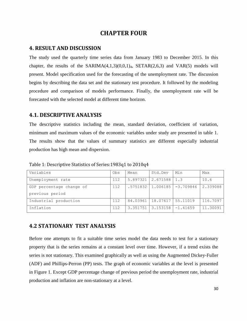
4.2 STATIONARY TEST ANALYSIS Before one attempts to fit a suitable time series model the data needs to test for a stationary

property that is the series remains at a constant level over time. However, if a trend exists the

series is not stationary. This examined graphically as well as using the Augmented Dickey-Fuller

(ADF) and Phillips-Perron (PP) tests. The graph of economic variables at the level is presented

in Figure 1. Except GDP percentage change of previous period the unemployment rate, industrial

production and inflation are non-stationary at a level.

31

24

68

10

UN

EMP

1985q1 1990q1 1995q1 2000q1 2005q1 2010q1time

Plot of unemployment rate

-4-2

02

GD

P

1985q1 1990q1 1995q1 2000q1 2005q1 2010q1time

plot of GDP percentage change of previous period

6080

100

120

IPR

OD

1985q1 1990q1 1995q1 2000q1 2005q1 2010q1time

Plot of Industrial production

-50

510

INF

1985q1 1990q1 1995q1 2000q1 2005q1 2010q1time

Plot of inflation rate

Figure 1: Time series plot of economic variables series at level

An important point to perform the ADF test is the specification of the lag order p. When p is

small, serial correlation of residuals will make the test biased, when p is too large the power of

the test will reduce. Therefore, choosing an optimal order of p is important to make the residuals

white noise. Accordingly, lags are chosen based on AIC, FPE, LR, and SBIC. Therefore, lag five

is chosen for the unemployment rate, lag three is chosen for gross domestic product, and lag two

is chosen for both industrial production and consumer price index. The result of ADF and PP

tests based on the chosen lags is presented in Table 2.

Table 2: Unit root test results (at constant time level)

Series Level with intercept Level with intercept and trend

Test

Statistics

Probab.* Test

Statistics

Probab.*

ADF PP ADF PP ADF PP ADF PP

Unemployment rate

-1.143 -1.267 0.697 0.6442 -1.580 -1.539 0.8718 0.8153

GDP percentage

change of

previous period

-4.095 -8.041 0.0010* 0.0000* -4.045 -8.007 0.0076* 0.0000*

IPRDO -1.280 -1.267 0.6384 0.6441 -2.816 -1.856 0.1913 0.6770

INF -2.766 -2.220 0.0633 0.1989 -3.383 -2.621 0.0537 0.2701

Critical value 5% -2.889 -3.449

32

The above table shows that values for the unemployment rate, industrial production, and

inflation are not more negative than the critical test which suggested the existence of unit root

test. Whereas, the gross domestic product is stationary. Therefore, both the graph and test

statistics reveals data variables except gross domestic product are none stationary.

However, in the Figure 1 unemployment series seems to have a structural break around 1991, for

some reason the unemployment rate have dramatically change after 1991. The presence of

structural break could make biased the result of standard unit root tests. The problem of standard

unit root tests is they do not allow a structural break. Consequently, when there is any structural

break in the data, the ADF and PP test is biased towards accepting of non-stationary because of

misspecification bias and size distortions. Therefore, to see whether standard unit root tests are

failed to reject the non-stationary hypothesis due to the existence of structural break in

unemployment rate series or not the test which allows the structural break has performed.

Table 3: Zivot-Andrews unit root test having structural break for unemployment rate

Series Allowing for break in trend Allowing for break in both

intercept and trend

Minimum

t-statistic

Critical values Minimum

t-statistic

Critical values

Unemployment rate 1% 5% 10% 1% 5% 10%

-2.567 -4.93 -4.42 -4.11 -3.592 -5.57 -5.08 -4.82

Potential break point at 1993Q4 Potential break point at 1991Q3

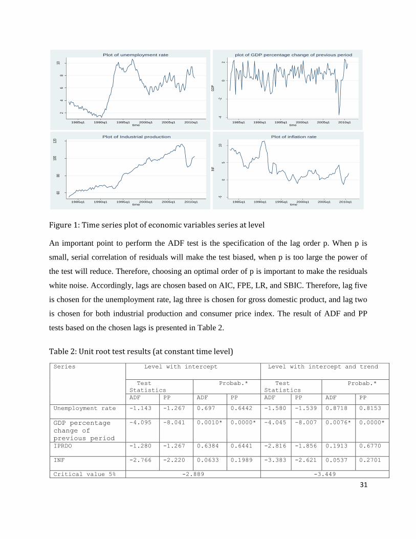
The Zivot test in Table 3 reveals there is no enough evidence to reject both null hypothesis of

unemployment has a unit root with structural break in trend, and in both intercept and trend.

-4

-3

-2

-1

0

1

Brea

kpoin

t t-sta

tistic

s

1985q1 1990q1 1995q1 2000q1 2005q1 2010q1time

Min breakpoint at 1991q3

Zivot-Andrews test for UNEMP, 1986q2-2008q1

Figure 2: Graphical presentation of structural break in intercept and trend.

33

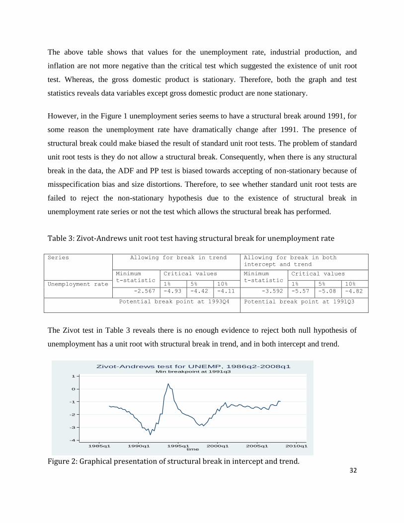
Consequently, unemployment rate, industrial production, and inflation need to be differenced.

The graph for the series of three variables after their first difference present in figure 2, shows

they are detrended.

-2-1

01

2

D.U

NE

MP

1985q1 1990q1 1995q1 2000q1 2005q1 2010q1time

Plot of differenced unemployment rate

-10

-50

5

D.IP

RO

D

1985q1 1990q1 1995q1 2000q1 2005q1 2010q1time

Plot of differenced Industrial production

-4-2

02

4

D.IN

F

1985q1 1990q1 1995q1 2000q1 2005q1 2010q1time

Plot of differenced inflation rate

Figure 3: Time series plots of economic variables at the first difference

Besides, the p-values for unemployment rate, industrial production, and inflation of ADF and PP

test in Table 4 is smaller than the 0.05. Consequently, the null hypothesis for both test is rejected,

series of those variables are stationary at their first difference.

Table-4: Unit root test results (after first difference)

Series Level with intercept Level with intercept and trend

Test Statistics Probab.* Test Statistics Probab.*

ADF PP ADF PP ADF PP ADF PP

Unemployment rate -3.879 -9.810 0.002 0.0000 -3.848 -9.771 0.014 0.0000

Industrial pro. -4.911 -7.036 0.0000 0.0000 -4.907 -7.030 0.0003 0.0000

Inflation -4.897 -7.859 0.0000 0.0000 -4.914 -7.854 0.0003 0.0000

Critical value 5% -2.889 -3.449

34

Furthermore, the unemployment rate series in Figure 1 reveals the existence of seasonal process

and after the series has differenced the process is clearer in Figure 2. Consequently, the study

turn to use the seasonal autoregressive integrated moving average (SARIMA) model instead of a

none-seasonal ARIMA. However, to deal with SARIMA model it requires to check whether the

seasonality is needed to be differenced or not. The existence of a structural break in series may

not only affect the level and trend of the series but it may also change the observed pattern of

seasonality. In this section the HEGY test (without structural breaks), for the null hypothesis of a

non-stationary seasonal cycle, is performed for the level series of the unemployment rate.

However, like non-seasonal unit root tests the HEGY test for seasonal unit root under a structural

break has less power it failed with a rejection of unit roots. Therefore, if the HEGY test without

structural breaks suggests that the series do not contain a unit root test, the HEGY test

considering structural breaks should not be carried out given that the former has more power

otherwise the study will proceed to perform HEGY test under the structural break.

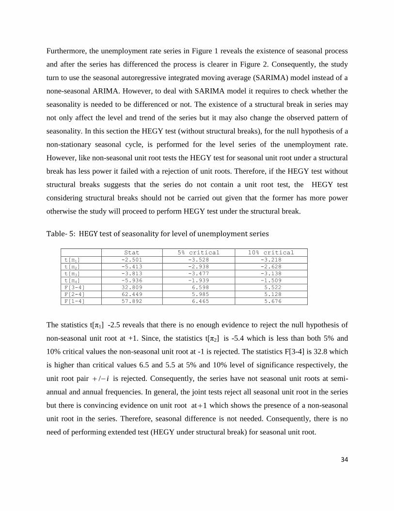
Table- 5: HEGY test of seasonality for level of unemployment series

Stat 5% critical 10% critical

t[π1] -2.501 -3.528 -3.218

t[π2] -5.413 -2.938 -2.628

t[π3] -3.813 -3.477 -3.138

t[π4] -5.936 -1.939 -1.509

F[3-4] 32.809 6.598 5.522

F[2-4] 62.449 5.985 5.128

F[1-4] 57.892 6.465 5.676

The statistics t[π1] -2.5 reveals that there is no enough evidence to reject the null hypothesis of

non-seasonal unit root at +1. Since, the statistics t[π2] is -5.4 which is less than both 5% and

10% critical values the non-seasonal unit root at -1 is rejected. The statistics F[3-4] is 32.8 which

is higher than critical values 6.5 and 5.5 at 5% and 10% level of significance respectively, the

unit root pair i / is rejected. Consequently, the series have not seasonal unit roots at semi-

annual and annual frequencies. In general, the joint tests reject all seasonal unit root in the series

but there is convincing evidence on unit root at 1 which shows the presence of a non-seasonal

unit root in the series. Therefore, seasonal difference is not needed. Consequently, there is no

need of performing extended test (HEGY under structural break) for seasonal unit root.

35

Consequently, time series process of the unemployment rate is integrated of order one. Thus, the

rate of unemployment will be modeled at the first difference of the series using different models

such as seasonal autoregressive integrated moving average model, self exciting threshold

autoregressive, and vector autoregressive models.

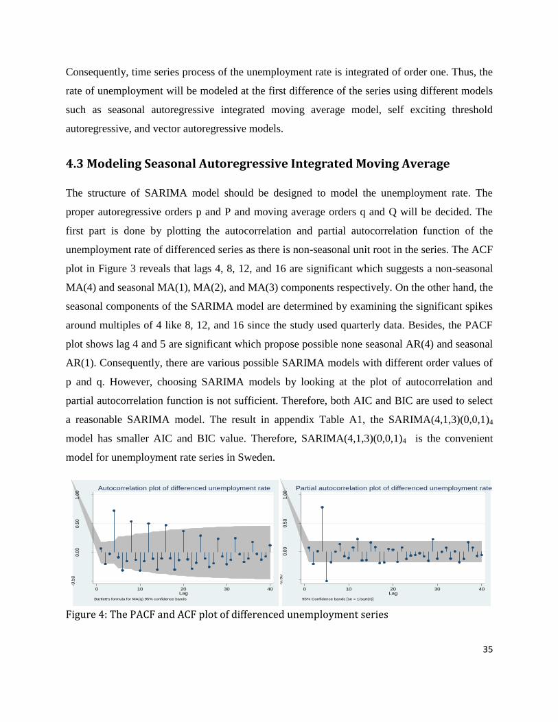
4.3 Modeling Seasonal Autoregressive Integrated Moving Average

The structure of SARIMA model should be designed to model the unemployment rate. The

proper autoregressive orders p and P and moving average orders q and Q will be decided. The

first part is done by plotting the autocorrelation and partial autocorrelation function of the

unemployment rate of differenced series as there is non-seasonal unit root in the series. The ACF

plot in Figure 3 reveals that lags 4, 8, 12, and 16 are significant which suggests a non-seasonal

MA(4) and seasonal MA(1), MA(2), and MA(3) components respectively. On the other hand, the

seasonal components of the SARIMA model are determined by examining the significant spikes

around multiples of 4 like 8, 12, and 16 since the study used quarterly data. Besides, the PACF

plot shows lag 4 and 5 are significant which propose possible none seasonal AR(4) and seasonal

AR(1). Consequently, there are various possible SARIMA models with different order values of

p and q. However, choosing SARIMA models by looking at the plot of autocorrelation and

partial autocorrelation function is not sufficient. Therefore, both AIC and BIC are used to select

a reasonable SARIMA model. The result in appendix Table A1, the SARIMA(4,1,3)(0,0,1)4

model has smaller AIC and BIC value. Therefore, SARIMA(4,1,3)(0,0,1)4 is the convenient

model for unemployment rate series in Sweden.

-0.5

00

.00

0.5

01

.00

Au

toco

rre

latio

ns

of D

.UN

EM

P

0 10 20 30 40Lag

Bartlett's formula for MA(q) 95% confidence bands

Autocorrelation plot of differenced unemployment rate

-0.5

00

.00

0.5

01

.00

Pa

rtia

l aut

oco

rrel

atio

ns o

f D.U

NE

MP

0 10 20 30 40Lag

95% Confidence bands [se = 1/sqrt(n)]

Partial autocorrelation plot of differenced unemployment rate

Figure 4: The PACF and ACF plot of differenced unemployment series

36

Once models have been applied to the data, the adequacy of the fit should be evaluated using

residual analysis. The portmanteau test of autocorrelation with lag eight in Table-6 suggest there

is no enough evidence to reject the null hypothesis of residual independence. Besides, the p-

values for Skewness, Kurtosis, and joint Jarque-Bera normality test of residuals is significantly

large, leading no enough evidence to reject the null hypothesis of residuals normality.

Table-6: Portmanteau with lag eight and JB test of residuals in SARIMA(4,1,3)(0,0,1)4

Type of test Test statistics Prob>chi2

Portmanteau (Q) statistic 2.52 0.96

Joint Jarque-Bera normality test 1.57 0.45

Pr(Skewness 0.37

Pr(Kurtosis) 0.39

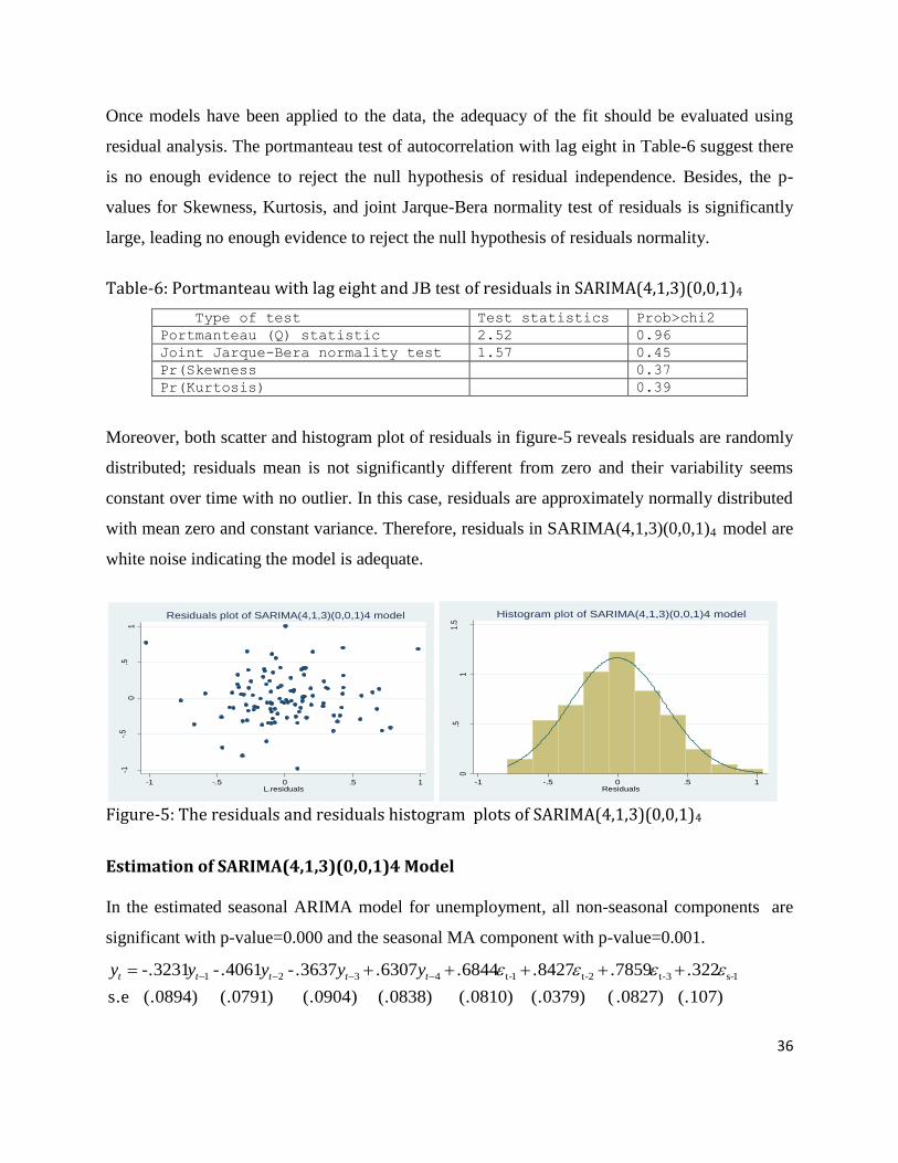
Moreover, both scatter and histogram plot of residuals in figure-5 reveals residuals are randomly

distributed; residuals mean is not significantly different from zero and their variability seems

constant over time with no outlier. In this case, residuals are approximately normally distributed

with mean zero and constant variance. Therefore, residuals in SARIMA(4,1,3)(0,0,1)4 model are

white noise indicating the model is adequate.

-1-.

50

.51

resi

dua

ls

-1 -.5 0 .5 1L.residuals

Residuals plot of SARIMA(4,1,3)(0,0,1)4 model

0.5

11.

5

Den

sity

-1 -.5 0 .5 1Residuals

Histogram plot of SARIMA(4,1,3)(0,0,1)4 model

Figure-5: The residuals and residuals histogram plots of SARIMA(4,1,3)(0,0,1)4

Estimation of SARIMA(4,1,3)(0,0,1)4 Model In the estimated seasonal ARIMA model for unemployment, all non-seasonal components are

significant with p-value=0.000 and the seasonal MA component with p-value=0.001.

(.107) .0827) ( (.0379) (.0810) (.0838) ) (.0904 ) (.0791 (.0894) s.e

.322.7859.8427 .6844.6307.3637-.4061- -.3231 1-s-3t2-t1-t4321 ttttt yyyyy

37

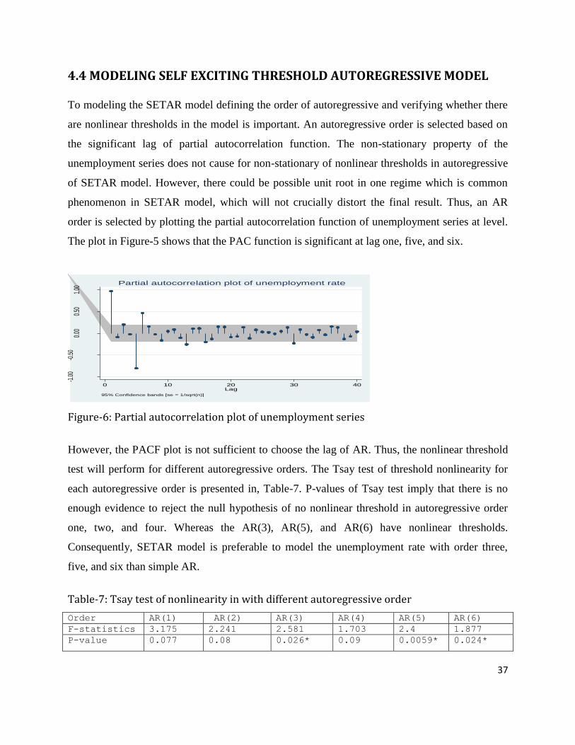
4.4 MODELING SELF EXCITING THRESHOLD AUTOREGRESSIVE MODEL To modeling the SETAR model defining the order of autoregressive and verifying whether there

are nonlinear thresholds in the model is important. An autoregressive order is selected based on

the significant lag of partial autocorrelation function. The non-stationary property of the

unemployment series does not cause for non-stationary of nonlinear thresholds in autoregressive

of SETAR model. However, there could be possible unit root in one regime which is common

phenomenon in SETAR model, which will not crucially distort the final result. Thus, an AR

order is selected by plotting the partial autocorrelation function of unemployment series at level.

The plot in Figure-5 shows that the PAC function is significant at lag one, five, and six.

-1.0

0-0

.50

0.00

0.50

1.00

Parti

al au

toco

rrelat

ions o

f UNE

MP

0 10 20 30 40Lag

95% Confidence bands [se = 1/sqrt(n)]

Partial autocorrelation plot of unemployment rate

Figure-6: Partial autocorrelation plot of unemployment series

However, the PACF plot is not sufficient to choose the lag of AR. Thus, the nonlinear threshold

test will perform for different autoregressive orders. The Tsay test of threshold nonlinearity for

each autoregressive order is presented in, Table-7. P-values of Tsay test imply that there is no

enough evidence to reject the null hypothesis of no nonlinear threshold in autoregressive order

one, two, and four. Whereas the AR(3), AR(5), and AR(6) have nonlinear thresholds.

Consequently, SETAR model is preferable to model the unemployment rate with order three,

five, and six than simple AR.

Table-7: Tsay test of nonlinearity in with different autoregressive order

Order AR(1) AR(2) AR(3) AR(4) AR(5) AR(6)

F-statistics 3.175 2.241 2.581 1.703 2.4 1.877

P-value 0.077 0.08 0.026* 0.09 0.0059* 0.024*

38

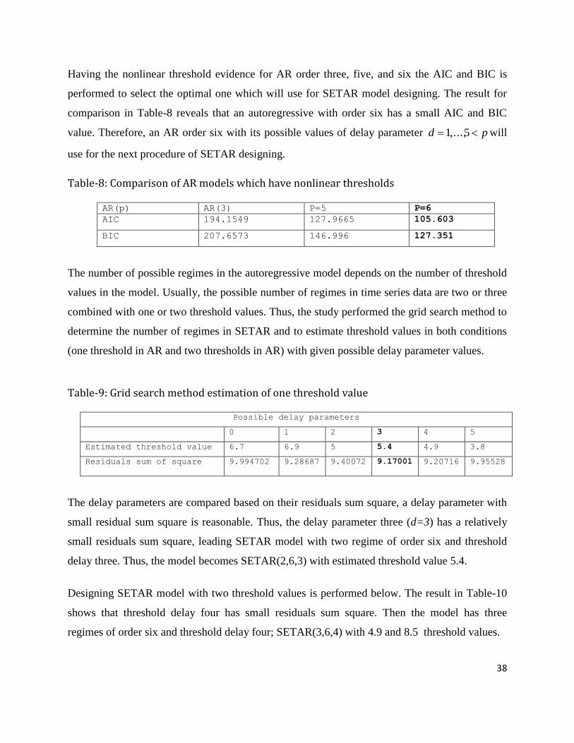
Having the nonlinear threshold evidence for AR order three, five, and six the AIC and BIC is

performed to select the optimal one which will use for SETAR model designing. The result for

comparison in Table-8 reveals that an autoregressive with order six has a small AIC and BIC

value. Therefore, an AR order six with its possible values of delay parameter pd 5,...,1 will

use for the next procedure of SETAR designing.

Table-8: Comparison of AR models which have nonlinear thresholds

AR(p) AR(3) P=5 P=6

AIC 194.1549 127.9665 105.603

BIC 207.6573 146.996 127.351

The number of possible regimes in the autoregressive model depends on the number of threshold

values in the model. Usually, the possible number of regimes in time series data are two or three

combined with one or two threshold values. Thus, the study performed the grid search method to

determine the number of regimes in SETAR and to estimate threshold values in both conditions

(one threshold in AR and two thresholds in AR) with given possible delay parameter values.

Table-9: Grid search method estimation of one threshold value

Possible delay parameters

0 1 2 3 4 5

Estimated threshold value 6.7 6.9 5 5.4 4.9 3.8

Residuals sum of square 9.994702 9.28687

9.40072 9.17001 9.20716 9.95528

The delay parameters are compared based on their residuals sum square, a delay parameter with

small residual sum square is reasonable. Thus, the delay parameter three (d=3) has a relatively

small residuals sum square, leading SETAR model with two regime of order six and threshold

delay three. Thus, the model becomes SETAR(2,6,3) with estimated threshold value 5.4.

Designing SETAR model with two threshold values is performed below. The result in Table-10

shows that threshold delay four has small residuals sum square. Then the model has three

regimes of order six and threshold delay four; SETAR(3,6,4) with 4.9 and 8.5 threshold values.

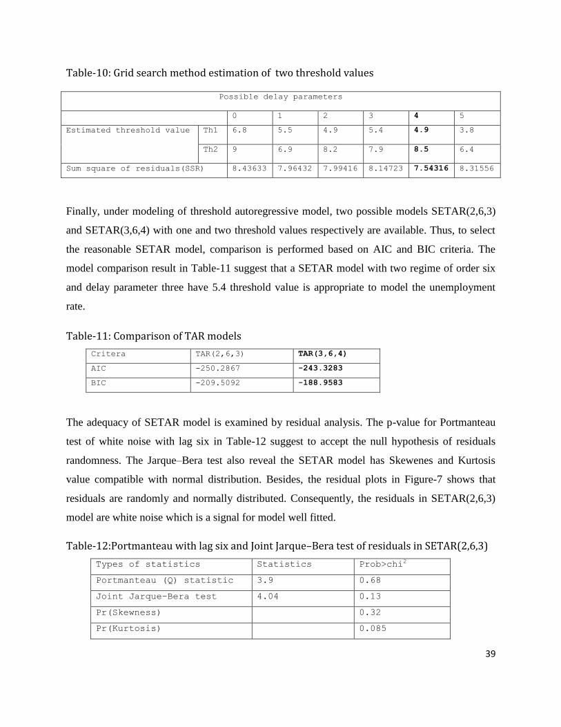
39

Table-10: Grid search method estimation of two threshold values

Possible delay parameters

0 1 2 3 4 5

Estimated threshold value Th1 6.8 5.5

4.9 5.4 4.9 3.8

Th2 9 6.9 8.2 7.9 8.5 6.4

Sum square of residuals(SSR) 8.43633 7.96432 7.99416 8.14723 7.54316 8.31556

Finally, under modeling of threshold autoregressive model, two possible models SETAR(2,6,3)

and SETAR(3,6,4) with one and two threshold values respectively are available. Thus, to select

the reasonable SETAR model, comparison is performed based on AIC and BIC criteria. The

model comparison result in Table-11 suggest that a SETAR model with two regime of order six

and delay parameter three have 5.4 threshold value is appropriate to model the unemployment

rate.

Table-11: Comparison of TAR models

Critera TAR(2,6,3) TAR(3,6,4)

AIC -250.2867 -243.3283

BIC -209.5092 -188.9583

The adequacy of SETAR model is examined by residual analysis. The p-value for Portmanteau

test of white noise with lag six in Table-12 suggest to accept the null hypothesis of residuals

randomness. The Jarque–Bera test also reveal the SETAR model has Skewenes and Kurtosis

value compatible with normal distribution. Besides, the residual plots in Figure-7 shows that

residuals are randomly and normally distributed. Consequently, the residuals in SETAR(2,6,3)

model are white noise which is a signal for model well fitted.

Table-12:Portmanteau with lag six and Joint Jarque–Bera test of residuals in SETAR(2,6,3)

Types of statistics Statistics Prob>chi2

Portmanteau (Q) statistic 3.9 0.68

Joint Jarque–Bera test 4.04 0.13

Pr(Skewness) 0.32

Pr(Kurtosis) 0.085

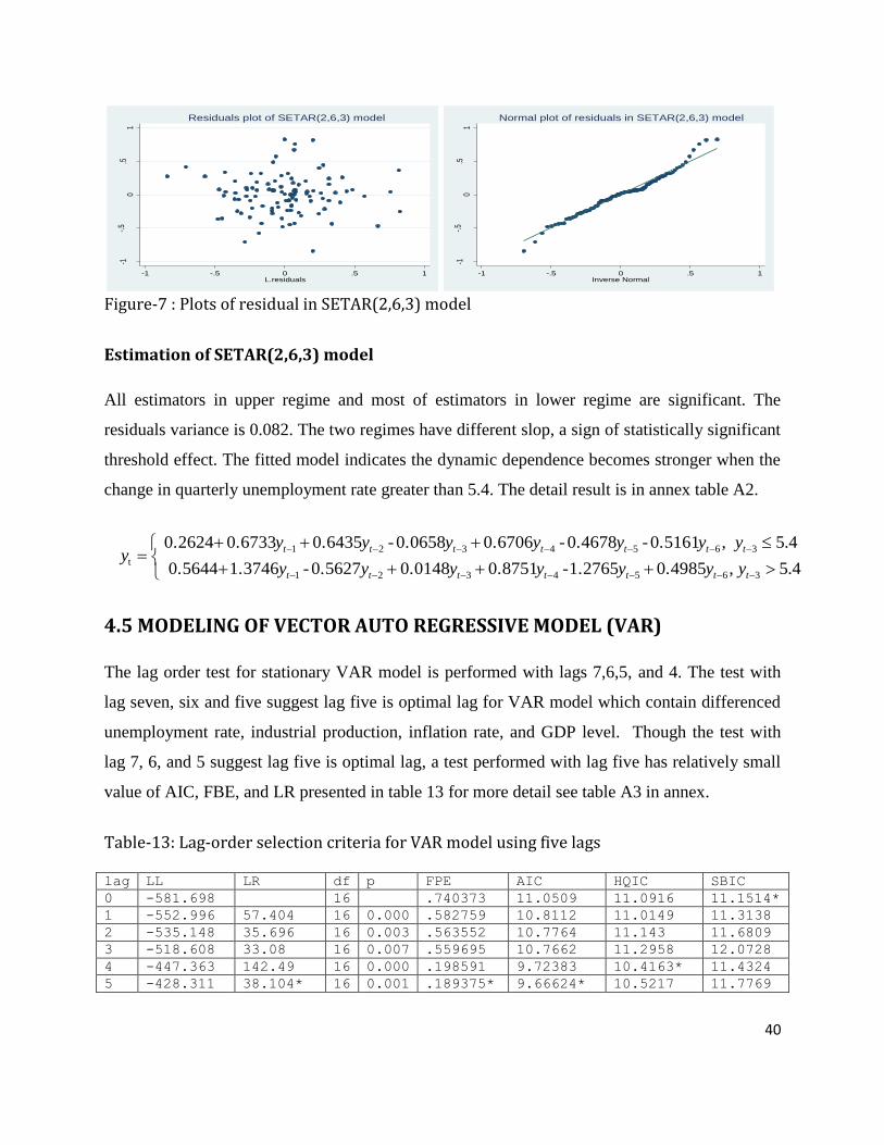
40

-1-.

50

.51

resi

dual

s

-1 -.5 0 .5 1L.residuals

Residuals plot of SETAR(2,6,3) model

-1-.

50

.51

resi

dual

s

-1 -.5 0 .5 1Inverse Normal

Normal plot of residuals in SETAR(2,6,3) model

Figure-7 : Plots of residual in SETAR(2,6,3) model

Estimation of SETAR(2,6,3) model

All estimators in upper regime and most of estimators in lower regime are significant. The

residuals variance is 0.082. The two regimes have different slop, a sign of statistically significant

threshold effect. The fitted model indicates the dynamic dependence becomes stronger when the

change in quarterly unemployment rate greater than 5.4. The detail result is in annex table A2.

4.5 ,0.49851.2765-0.8751 0.0148 0.5627-1.37460.5644

4.5 ,0.5161-0.4678-0.67060.0658-0.64350.67330.2624

3654321

3654321

t

ttttttt

ttttttt

yyyyyyy

yyyyyyy y

4.5 MODELING OF VECTOR AUTO REGRESSIVE MODEL (VAR)

The lag order test for stationary VAR model is performed with lags 7,6,5, and 4. The test with

lag seven, six and five suggest lag five is optimal lag for VAR model which contain differenced

unemployment rate, industrial production, inflation rate, and GDP level. Though the test with

lag 7, 6, and 5 suggest lag five is optimal lag, a test performed with lag five has relatively small

value of AIC, FBE, and LR presented in table 13 for more detail see table A3 in annex.

Table-13: Lag-order selection criteria for VAR model using five lags lag LL LR df p FPE AIC HQIC SBIC

0 -581.698 16 .740373 11.0509 11.0916 11.1514*

1 -552.996 57.404 16 0.000 .582759 10.8112 11.0149 11.3138

2 -535.148 35.696 16 0.003 .563552 10.7764 11.143 11.6809

3 -518.608 33.08 16 0.007 .559695 10.7662 11.2958 12.0728

4 -447.363 142.49 16 0.000 .198591 9.72383 10.4163* 11.4324

5 -428.311 38.104* 16 0.001 .189375* 9.66624* 10.5217 11.7769

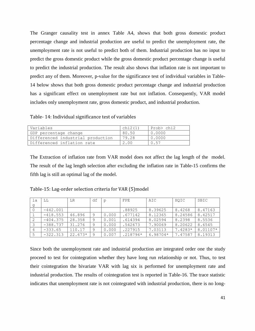
41

The Granger causality test in annex Table A4, shows that both gross domestic product

percentage change and industrial production are useful to predict the unemployment rate, the

unemployment rate is not useful to predict both of them. Industrial production has no input to

predict the gross domestic product while the gross domestic product percentage change is useful

to predict the industrial production. The result also shows that inflation rate is not important to

predict any of them. Moreover, p-value for the significance test of individual variables in Table-

14 below shows that both gross domestic product percentage change and industrial production

has a significant effect on unemployment rate but not inflation. Consequently, VAR model

includes only unemployment rate, gross domestic product, and industrial production.

Table- 14: Individual significance test of variables Variables chi2(1) Prob> chi2

GDP percentage change 80.50 0.0000

Differenced industrial production 79.28 0.0000

Differenced inflation rate 2.00 0.57

The Extraction of inflation rate from VAR model does not affect the lag length of the model.

The result of the lag length selection after excluding the inflation rate in Table-15 confirms the

fifth lag is still an optimal lag of the model.

Table-15: Lag-order selection criteria for VAR (5)model la

g

LL LR df p FPE AIC HQIC SBIC

0 -442.001 .88925 8.39625 8.4268 8.47163

1 -418.553 46.896 9 0.000 .677142 8.12365 8.24586 8.42517

2 -404.375 28.358 9 0.001 .614394 8.02594 8.2398 8.5536

3 -388.737 31.276 9 0.000 .542673 7.90069 8.20622 8.6545

4 -333.65 110.17 9 0.000 .227915 7.03113 7.4283* 8.01107*

5 -322.313 22.673* 9 0.007 .218796* 6.98704* 7.47587 8.19313

Since both the unemployment rate and industrial production are integrated order one the study

proceed to test for cointegration whether they have long run relationship or not. Thus, to test

their cointegration the bivariate VAR with lag six is performed for unemployment rate and

industrial production. The results of cointegration test is reported in Table-16. The trace statistic

indicates that unemployment rate is not cointegrated with industrial production, there is no long-

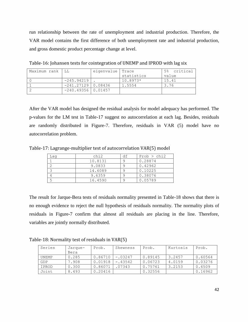
42

run relationship between the rate of unemployment and industrial production. Therefore, the

VAR model contains the first difference of both unemployment rate and industrial production,

and gross domestic product percentage change at level.

Table-16: Johansen tests for cointegration of UNEMP and IPROD with lag six

Maximum rank LL eigenvalue Trace

statistics

5% critical

value

0 -245.94219 . 10.8973* 15.41

1 -241.27129 0.08436 1.5554 3.76

2 -240.49356 0.01457

After the VAR model has designed the residual analysis for model adequacy has performed. The

p-values for the LM test in Table-17 suggest no autocorrelation at each lag. Besides, residuals

are randomly distributed in Figure-7. Therefore, residuals in VAR (5) model have no

autocorrelation problem.

Table-17: Lagrange-multiplier test of autocorrelation VAR(5) model

Lag chi2 df Prob > chi2

1 10.8131 9 0.28874

2 9.0833 9 0.42962

3 14.6089 9 0.10225

4 9.6359 9 0.38076

5 16.4590 9 0.05789

The result for Jarque-Bera tests of residuals normality presented in Table-18 shows that there is

no enough evidence to reject the null hypothesis of residuals normality. The normality plots of

residuals in Figure-7 confirm that almost all residuals are placing in the line. Therefore,

variables are jointly normally distributed.

Table-18: Normality test of residuals in VAR(5)

Series Jarque-

Bera

Prob. Skewness Prob. Kurtosis Prob.

UNEMP 0.285 0.86710 -.03247 0.89145 3.2457 0.60564

GDP 7.908 0.01918 -.43542 0.06723 4.0159 0.03276

IPROD 0.300 0.86071 .07343 0.75761 3.2153 0.6509

Joint 8.493 0.20416 0.32556 0.16962

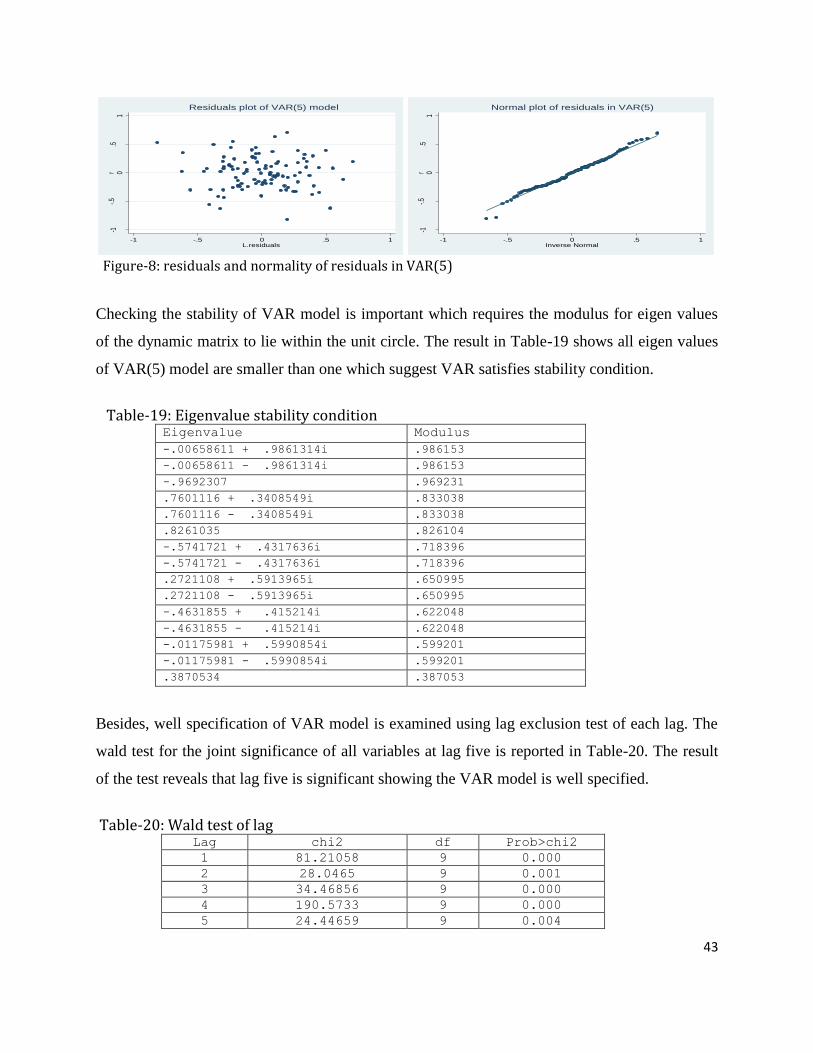
43

-1-.5

0.5

1r

-1 -.5 0 .5 1L.residuals

Residuals plot of VAR(5) model

-1-.5

0.5

1r

-1 -.5 0 .5 1Inverse Normal

Normal plot of residuals in VAR(5)

Figure-8: residuals and normality of residuals in VAR(5)

Checking the stability of VAR model is important which requires the modulus for eigen values

of the dynamic matrix to lie within the unit circle. The result in Table-19 shows all eigen values

of VAR(5) model are smaller than one which suggest VAR satisfies stability condition.

Table-19: Eigenvalue stability condition Eigenvalue Modulus -.00658611 + .9861314i .986153

-.00658611 - .9861314i .986153

-.9692307 .969231

.7601116 + .3408549i .833038

.7601116 - .3408549i .833038

.8261035 .826104

-.5741721 + .4317636i .718396

-.5741721 - .4317636i .718396

.2721108 + .5913965i .650995

.2721108 - .5913965i .650995

-.4631855 + .415214i .622048

-.4631855 - .415214i .622048

-.01175981 + .5990854i .599201

-.01175981 - .5990854i .599201

.3870534 .387053

Besides, well specification of VAR model is examined using lag exclusion test of each lag. The

wald test for the joint significance of all variables at lag five is reported in Table-20. The result

of the test reveals that lag five is significant showing the VAR model is well specified.

Table-20: Wald test of lag Lag chi2 df Prob>chi2

1 81.21058 9 0.000

2 28.0465 9 0.001

3 34.46856 9 0.000

4 190.5733 9 0.000

5 24.44659 9 0.004

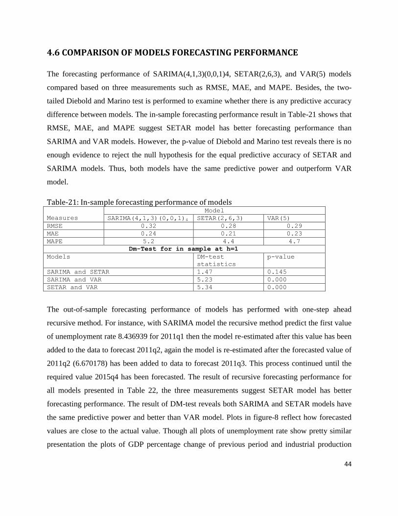
44

4.6 COMPARISON OF MODELS FORECASTING PERFORMANCE

The forecasting performance of SARIMA(4,1,3)(0,0,1)4, SETAR(2,6,3), and VAR(5) models

compared based on three measurements such as RMSE, MAE, and MAPE. Besides, the two-

tailed Diebold and Marino test is performed to examine whether there is any predictive accuracy

difference between models. The in-sample forecasting performance result in Table-21 shows that

RMSE, MAE, and MAPE suggest SETAR model has better forecasting performance than

SARIMA and VAR models. However, the p-value of Diebold and Marino test reveals there is no

enough evidence to reject the null hypothesis for the equal predictive accuracy of SETAR and

SARIMA models. Thus, both models have the same predictive power and outperform VAR

model.

Table-21: In-sample forecasting performance of models

Measures

Model

SARIMA(4,1,3)(0,0,1)4 SETAR(2,6,3) VAR(5)

RMSE 0.32 0.28 0.29

MAE 0.24 0.21 0.23

MAPE 5.2 4.4 4.7

Dm-Test for in sample at h=1

Models DM-test

statistics

p-value

SARIMA and SETAR 1.47 0.145

SARIMA and VAR 5.23 0.000

SETAR and VAR 5.34 0.000

The out-of-sample forecasting performance of models has performed with one-step ahead

recursive method. For instance, with SARIMA model the recursive method predict the first value

of unemployment rate 8.436939 for 2011q1 then the model re-estimated after this value has been

added to the data to forecast 2011q2, again the model is re-estimated after the forecasted value of

2011q2 (6.670178) has been added to data to forecast 2011q3. This process continued until the

required value 2015q4 has been forecasted. The result of recursive forecasting performance for

all models presented in Table 22, the three measurements suggest SETAR model has better

forecasting performance. The result of DM-test reveals both SARIMA and SETAR models have

the same predictive power and better than VAR model. Plots in figure-8 reflect how forecasted

values are close to the actual value. Though all plots of unemployment rate show pretty similar

presentation the plots of GDP percentage change of previous period and industrial production

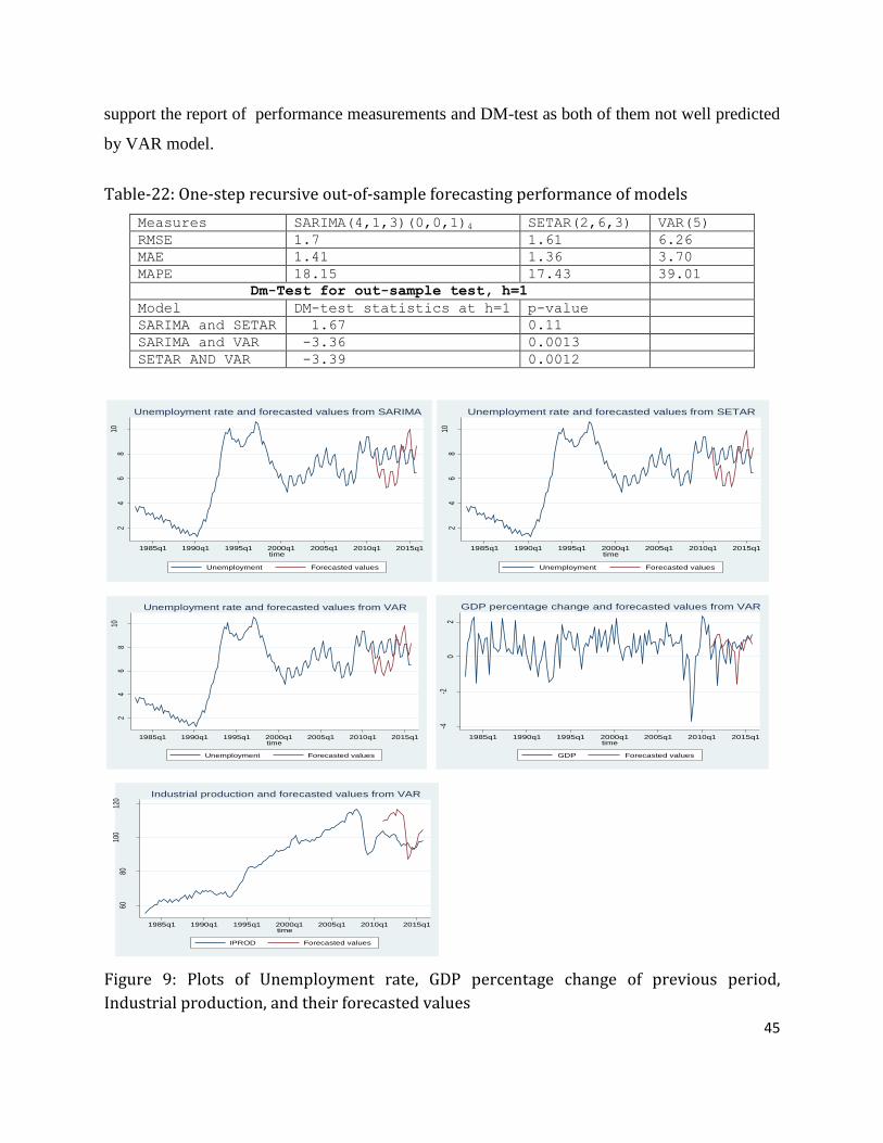
45

support the report of performance measurements and DM-test as both of them not well predicted

by VAR model.

Table-22: One-step recursive out-of-sample forecasting performance of models

Measures SARIMA(4,1,3)(0,0,1)4 SETAR(2,6,3) VAR(5)

RMSE 1.7 1.61 6.26

MAE 1.41 1.36 3.70

MAPE 18.15 17.43 39.01

Dm-Test for out-sample test, h=1

Model DM-test statistics at h=1 p-value

SARIMA and SETAR 1.67 0.11

SARIMA and VAR -3.36 0.0013

SETAR AND VAR -3.39 0.0012

24

68

10

1985q1 1990q1 1995q1 2000q1 2005q1 2010q1 2015q1time

Unemployment Forecasted values

Unemployment rate and forecasted values from SARIMA

24

68

10

1985q1 1990q1 1995q1 2000q1 2005q1 2010q1 2015q1time

Unemployment Forecasted values

Unemployment rate and forecasted values from SETAR

24

68

10

1985q1 1990q1 1995q1 2000q1 2005q1 2010q1 2015q1time

Unemployment Forecasted values

Unemployment rate and forecasted values from VAR

-4-2

02

1985q1 1990q1 1995q1 2000q1 2005q1 2010q1 2015q1time

GDP Forecasted values

GDP percentage change and forecasted values from VAR

6080

100

120

1985q1 1990q1 1995q1 2000q1 2005q1 2010q1 2015q1time

IPROD Forecasted values

Industrial production and forecasted values from VAR

Figure 9: Plots of Unemployment rate, GDP percentage change of previous period,

Industrial production, and their forecasted values

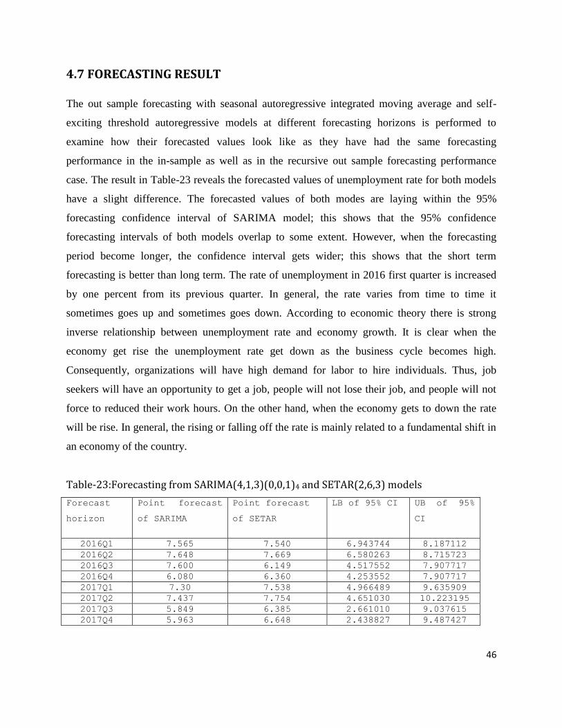
46

4.7 FORECASTING RESULT

The out sample forecasting with seasonal autoregressive integrated moving average and self-

exciting threshold autoregressive models at different forecasting horizons is performed to

examine how their forecasted values look like as they have had the same forecasting

performance in the in-sample as well as in the recursive out sample forecasting performance

case. The result in Table-23 reveals the forecasted values of unemployment rate for both models

have a slight difference. The forecasted values of both modes are laying within the 95%

forecasting confidence interval of SARIMA model; this shows that the 95% confidence

forecasting intervals of both models overlap to some extent. However, when the forecasting

period become longer, the confidence interval gets wider; this shows that the short term

forecasting is better than long term. The rate of unemployment in 2016 first quarter is increased

by one percent from its previous quarter. In general, the rate varies from time to time it

sometimes goes up and sometimes goes down. According to economic theory there is strong

inverse relationship between unemployment rate and economy growth. It is clear when the

economy get rise the unemployment rate get down as the business cycle becomes high.

Consequently, organizations will have high demand for labor to hire individuals. Thus, job

seekers will have an opportunity to get a job, people will not lose their job, and people will not

force to reduced their work hours. On the other hand, when the economy gets to down the rate

will be rise. In general, the rising or falling off the rate is mainly related to a fundamental shift in

an economy of the country.

Table-23:Forecasting from SARIMA(4,1,3)(0,0,1)4 and SETAR(2,6,3) models

Forecast

horizon

Point forecast

of SARIMA

Point forecast

of SETAR

LB of 95% CI UB of 95%

CI

2016Q1 7.565 7.540 6.943744 8.187112

2016Q2 7.648 7.669 6.580263 8.715723

2016Q3 7.600 6.149 4.517552 7.907717

2016Q4 6.080 6.360 4.253552 7.907717

2017Q1 7.30 7.538 4.966489 9.635909

2017Q2 7.437 7.754 4.651030 10.223195

2017Q3 5.849 6.385 2.661010 9.037615

2017Q4 5.963 6.648 2.438827 9.487427

47

CHAPER FIVE

CONCLUSION and RECOMENDATION

5.1 CONCLUSION

Modeling the unemployment rate in Sweden is performed using both univariate and multivariate

time series models namely SARIMA, SETAR, and VAR. All models are well fitted and

adequate. The combined modeling process shows unemployment rate is nonstationary nonlinear.

The rate also has stationary seasonal nature. The predictive accuracy performance of models in

both in-sample and one-step recursive out-of-sample forecasting performance methods is

measured based on the performance measures (RMSE, MAE, and MAPE) as well as Diebold and

Marino test. The performance measures for both in-sample and recursive out-of-sample methods

shows SETAR model is best forecasting model. The Diebold-Mariano test at one forecast

horizon for both in-sample and recursive out-sample methods reveals that the SARIMA and

SETAR models have the same forecasting performance and better than the VAR model.

Finding of forecasting accuracy for both linear and nonlinear models support the study done by

Join(1999) for UK and Power and Gasser(2012) for Canada unemployment rate.

All predicted values of both models are placing within the 95% forecasting confidence interval

of SARIMA model. The finding also suggests the short-term is better than long-term forecasting.

5.2 RECOMMENDATION

As short-term forecasting is better, there should be a continuous examination of an appropriate

model which used to predict the future values of the unemployment rate. Further investigations

on both simple and complex econometric models are essential, thus, the long-run unemployment

rates could be predicted as well.

Modeling the seasonal nature of unemployment rate in the nonlinear framework and modeling

the unemployment rate using structural VAR model can be a point of interest for future research.

48

REFERENCE

Britt CL 1994. Crime and Unemployment among Youth in the United States, 1958-1990.

American Journal of Economics and Sociology, 53(1): 99-109.

Clements, M. P., & Hendry, D. F. (2003). On the limitations of comparing mean squared forecast

errors (with discussion). Journal of Forecasting, 12, 617–639.

Diebold, F. X. & Mariano, R. S. 1995. Comparing Predictive Accuracy. Journal of Business &

Economic Statistics, 13, 253-263.

Economy Trade (2016): Retrieved from http://www.tradingeconomics.com/sweden/ unemployment -rate

Engle, R. F. and Granger, C. W. (1987): “Cointegration and Error Correction: Representation,

Estimation and Testing”. Econometrica, 55,251-276.

Ette H., Uchendu B, and Uyodhu V (2012): “Arima Fit to Nigerian Unemployment Data”. Journal of Basic and Applied Scientific Research, 2(6)5964-5970 ISSN 2090-4304.

Gil-Alana, L. A. (2001): “A fractionally Integrated Exponential Model for UK Unemployment”, Journal of Forecasting, 20, 329-340.

Hamilton, J.D. (1994): Time Series Analysis. Princeton University Press, Princeton.

Hammarstrom A, Janlert U 1997. Nervous and Depressive Symptoms in a Longitudinal Study of

Youth Unemployment-Selection or Exposure?. Journal of Adolescence, 20(3): 293-305.

Hylleberg, S., Engle, R.F., Granger, C.W.J. & Yoo, S. (1990). Seasonal integration and

cointegration. Journal of Econometrics, 44, 215–238.

Johnes, G. (1999): “Forecasting Unemployment”, Applied Financial Economics, 6, 605-607.

Kishor, N. K., & Koenig E. F. (2012).VAR estimation and forecasting when data are subject to

revision. Journal of Business & Economic Statistics, 30(2), 181–190.

Koop, G. and Potter, S. M. (1999): “Dynamic Asymmetries in U.S. Unemployment”, Journal of

Business and Economic Statistics, 17, 298-312.

Lack ,C. (2006): “Forecasting Swiss inflation using VAR models”. Swiss National Bank

Economic Studies, No. 2 2006

49

Lutkepohl, H. (1991): Introduction to Multiple Time Series Analysis .Springer-Verlag, Berlin.

Parker, R. E. and Rothman, P. (1998): “The Current Depth-of-Recession and Unemployment

Rate Forecasts”, Studies in Nonlinear Dynamics and Econometrics, 2, 151-158.

Peel, D. A. and Speight, A. E. H. (2000): “Threshold Nonlinearities in Unemployment Rates:

Further Evidence for the UK and G3 Economies”, Applied Economics, 32, 705-715.

Phillips, P. C. & Perron, P. 1988. Testing for a unit root in time series regression. Biometrika, 75,

335-346.

Power, B. and Gasser, K. (2012): “Forecasting Future Unemployment Rates”. ECON 452 First

Report.

Proietti, T. (2001): “Forecasting the US Unemployment Rate”, Working Paper.

Reynolds GL 2000. Unemployment and Drug Use. American Indian and Alasha-Native Mental

Health Research, 9(1): 17-23.

Robinson, W. (1998). Forecasting inflation using VAR Analysis.Bank of Jamaica.

Rothman, P. (1998): “Forecasting Asymmetric Unemployment Rates”, Review of Economics

and Statistics, 80, 164-168.

Skalin J., Terasvirta T., 1999, Modelling asymmetries and moving equilibria in unemployment

rates, Workeing Paper Series in Economic and Finance n.262, Stockholm School of Economics.

Tsay, R.S., (1989). “Testing and Modeling Threshold Autoregressive Processes”, Journal of the

American Statistical Association, 84(405), 231-240.

Tsay, R. S. 2005. Analysis of financial time series, John Wiley & Sons.

Weich S, Lewis G. 1998. Poverty, Unemployment and Common Mental Disorder: Population-

based Chart Study. British Medical Journal, 317: 115-119.

Zivot, E. and D. Andrews, (1992), Further evidence of great crash, the oil price shock and

unit root hypothesis, Journal of Business and Economic Statistics, 10, 251-270.

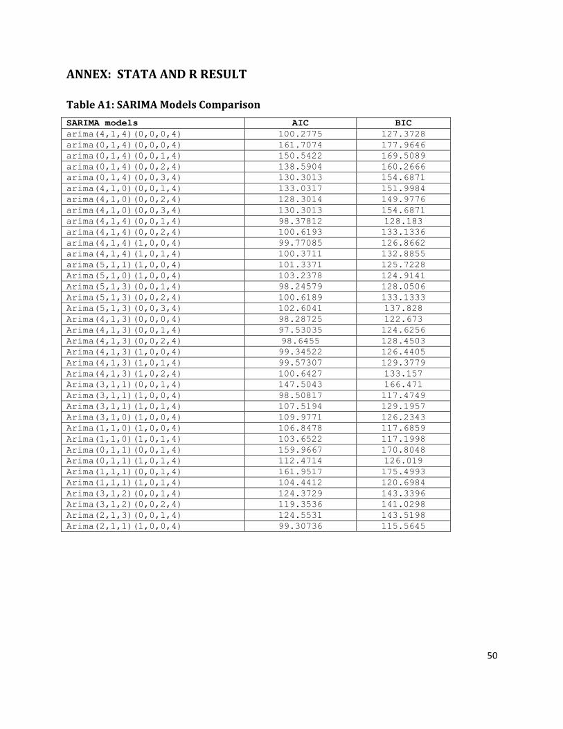
50

ANNEX: STATA AND R RESULT

Table A1: SARIMA Models Comparison

SARIMA models AIC BIC

arima(4,1,4)(0,0,0,4) 100.2775 127.3728

arima(0,1,4)(0,0,0,4) 161.7074 177.9646

arima(0,1,4)(0,0,1,4) 150.5422 169.5089

arima(0,1,4)(0,0,2,4) 138.5904 160.2666

arima(0,1,4)(0,0,3,4) 130.3013 154.6871

arima(4,1,0)(0,0,1,4) 133.0317 151.9984

arima(4,1,0)(0,0,2,4) 128.3014 149.9776

arima(4,1,0)(0,0,3,4) 130.3013 154.6871

arima(4,1,4)(0,0,1,4) 98.37812 128.183

arima(4,1,4)(0,0,2,4) 100.6193 133.1336

arima(4,1,4)(1,0,0,4) 99.77085 126.8662

arima(4,1,4)(1,0,1,4) 100.3711 132.8855

arima(5,1,1)(1,0,0,4) 101.3371 125.7228

Arima(5,1,0)(1,0,0,4) 103.2378 124.9141

Arima(5,1,3)(0,0,1,4) 98.24579 128.0506

Arima(5,1,3)(0,0,2,4) 100.6189 133.1333

Arima(5,1,3)(0,0,3,4) 102.6041 137.828

Arima(4,1,3)(0,0,0,4) 98.28725 122.673

Arima(4,1,3)(0,0,1,4) 97.53035 124.6256

Arima(4,1,3)(0,0,2,4) 98.6455 128.4503

Arima(4,1,3)(1,0,0,4) 99.34522 126.4405

Arima(4,1,3)(1,0,1,4) 99.57307 129.3779

Arima(4,1,3)(1,0,2,4) 100.6427 133.157

Arima(3,1,1)(0,0,1,4) 147.5043 166.471

Arima(3,1,1)(1,0,0,4) 98.50817 117.4749

Arima(3,1,1)(1,0,1,4) 107.5194 129.1957

Arima(3,1,0)(1,0,0,4) 109.9771 126.2343

Arima(1,1,0)(1,0,0,4) 106.8478 117.6859

Arima(1,1,0)(1,0,1,4) 103.6522 117.1998

Arima(0,1,1)(0,0,1,4) 159.9667 170.8048

Arima(0,1,1)(1,0,1,4) 112.4714 126.019

Arima(1,1,1)(0,0,1,4) 161.9517 175.4993

Arima(1,1,1)(1,0,1,4) 104.4412 120.6984

Arima(3,1,2)(0,0,1,4) 124.3729 143.3396

Arima(3,1,2)(0,0,2,4) 119.3536 141.0298

Arima(2,1,3)(0,0,1,4) 124.5531 143.5198

Arima(2,1,1)(1,0,0,4) 99.30736 115.5645

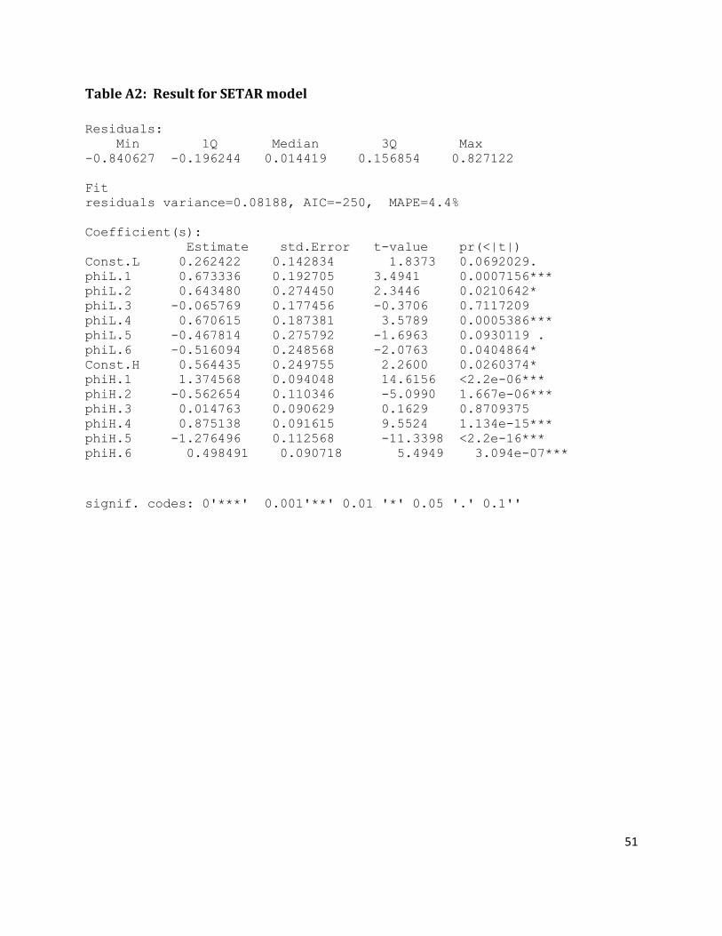
51

Table A2: Result for SETAR model

Residuals:

Min 1Q Median 3Q Max

-0.840627 -0.196244 0.014419 0.156854 0.827122

Fit

residuals variance=0.08188, AIC=-250, MAPE=4.4%

Coefficient(s):

Estimate std.Error t-value pr(<|t|)

Const.L 0.262422 0.142834 1.8373 0.0692029.

phiL.1 0.673336 0.192705 3.4941 0.0007156***

phiL.2 0.643480 0.274450 2.3446 0.0210642*

phiL.3 -0.065769 0.177456 -0.3706 0.7117209

phiL.4 0.670615 0.187381 3.5789 0.0005386***

phiL.5 -0.467814 0.275792 -1.6963 0.0930119 .

phiL.6 -0.516094 0.248568 -2.0763 0.0404864*

Const.H 0.564435 0.249755 2.2600 0.0260374*

phiH.1 1.374568 0.094048 14.6156 <2.2e-06***

phiH.2 -0.562654 0.110346 -5.0990 1.667e-06***

phiH.3 0.014763 0.090629 0.1629 0.8709375

phiH.4 0.875138 0.091615 9.5524 1.134e-15***

phiH.5 -1.276496 0.112568 -11.3398 <2.2e-16***

phiH.6 0.498491 0.090718 5.4949 3.094e-07*** signif. codes: 0'***' 0.001'**' 0.01 '*' 0.05 '.' 0.1''

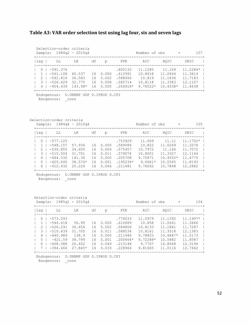
52

Table A3: VAR order selection test using lag four, six and seven lags

Selection-order criteria

Sample: 1984q2 - 2010q4 Number of obs = 107

+---------------------------------------------------------------------------+

|lag | LL LR df p FPE AIC HQIC SBIC |

|----+----------------------------------------------------------------------|

| 0 | -591.376 .800132 11.1285 11.169 11.2284* |

| 1 | -561.108 60.537 16 0.000 .612991 10.8618 11.0644 11.3614 |

| 2 | -542.816 36.583 16 0.002 .588066 10.819 11.1836 11.7183 |

| 3 | -526.429 32.775 16 0.008 .585714 10.8118 11.3383 12.1107 |

| 4 | -454.439 143.98* 16 0.000 .206918* 9.76522* 10.4538* 11.4638 |

+---------------------------------------------------------------------------+

Endogenous: D.UNEMP GDP D.IPROD D.CPI

Exogenous: _cons

Selection-order criteria

Sample: 1984q4 - 2010q4 Number of obs = 105

+---------------------------------------------------------------------------+

|lag | LL LR df p FPE AIC HQIC SBIC |

|----+----------------------------------------------------------------------|

| 0 | -577.125 .753929 11.069 11.11 11.1702* |

| 1 | -548.157 57.936 16 0.000 .589086 10.822 11.0269 11.3276 |

| 2 | -530.855 34.605 16 0.004 .575457 10.7972 11.166 11.7072 |

| 3 | -515.004 31.701 16 0.011 .579074 10.8001 11.3327 12.1144 |

| 4 | -444.332 141.34 16 0.000 .205708 9.75871 10.4552* 11.4775 |

| 5 | -425.045 38.574* 16 0.001 .195236* 9.6961* 10.5565 11.8193 |

| 6 | -412.432 25.226 16 0.066 .211481 9.76062 10.7848 12.2882 |

+---------------------------------------------------------------------------+

Endogenous: D.UNEMP GDP D.IPROD D.CPI

Exogenous: _cons

Selection-order criteria

Sample: 1985q1 - 2010q4 Number of obs = 104

+---------------------------------------------------------------------------+

|lag | LL LR df p FPE AIC HQIC SBIC |

|----+----------------------------------------------------------------------|

| 0 | -573.093 .776033 11.0979 11.1392 11.1997* |

| 1 | -544.618 56.95 16 0.000 .610689 10.858 11.0641 11.3666 |

| 2 | -526.291 36.654 16 0.002 .584806 10.8133 11.1841 11.7287 |

| 3 | -510.439 31.705 16 0.011 .588534 10.8161 11.3518 12.1383 |

| 4 | -440.989 138.9 16 0.000 .211946 9.78825 10.4887* 11.5173 |

| 5 | -421.59 38.799 16 0.001 .200664* 9.72288* 10.5882 11.8587 |

| 6 | -408.388 26.402 16 0.049 .215148 9.7767 10.8068 12.3194 |

| 7 | -394.466 27.845* 16 0.033 .228966 9.81665 11.0116 12.7662 |

+---------------------------------------------------------------------------+

Endogenous: D.UNEMP GDP D.IPROD D.CPI

Exogenous: _cons

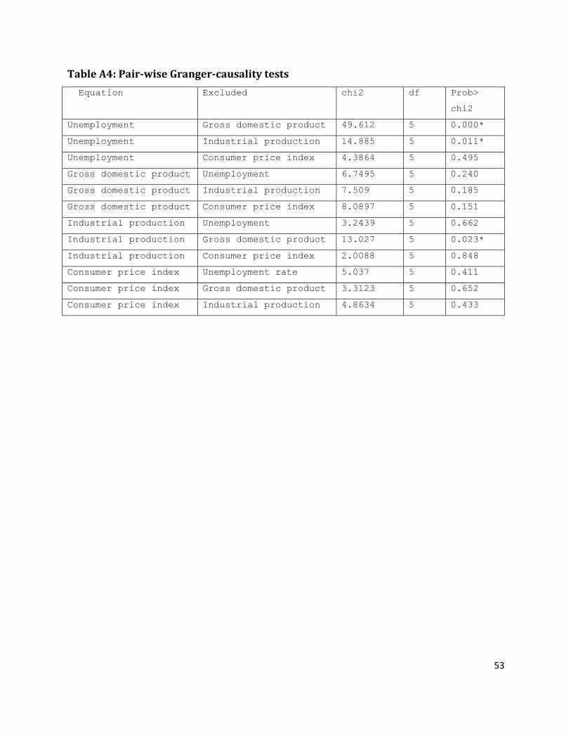
53

Table A4: Pair-wise Granger-causality tests

Equation Excluded chi2 df Prob>

chi2

Unemployment Gross domestic product 49.612 5 0.000*

Unemployment Industrial production 14.885 5 0.011*

Unemployment Consumer price index 4.3864 5 0.495

Gross domestic product Unemployment 6.7495 5 0.240

Gross domestic product Industrial production 7.509 5 0.185

Gross domestic product Consumer price index 8.0897 5 0.151

Industrial production Unemployment 3.2439 5 0.662

Industrial production Gross domestic product 13.027 5 0.023*

Industrial production Consumer price index 2.0088 5 0.848

Consumer price index Unemployment rate 5.037 5 0.411

Consumer price index Gross domestic product 3.3123 5 0.652

Consumer price index Industrial production 4.8634 5 0.433