Modeling and Forecasting the Volatility of Oil Futures Using the ARCH ... · PDF fileModeling...

The Lahore Journal of Business 1:1 (Summer 2012): pp. 79–108

Modeling and Forecasting the Volatility of Oil Futures Using the ARCH Family Models

Tareena Musaddiq∗

Abstract

This study attempts to model and forecast the volatility of light, sweet, crude oil futures trading at the NYMEX during 1998–2009, using various models from the ARCH family. The results reveal that the GJR-GARCH (1,2) model is best suited to forecast purposes. The fitted models also suggest the presence of asymmetric effects in the data. The study also reveals that trading volume and open interest do not reduce the persistence of volatility for these oil futures.

Keywords: Modeling volatility, forecasting, oil futures.

Classification: C53, C58, G17.

1. Introduction

Extensive research has been conducted on modeling volatility clustering in financial markets, using different econometric techniques. Volatility modeling is a key area of interest to researchers because it plays an important role in managing risk, pricing derivatives, hedging, selecting portfolios, and policymaking. “Investors and portfolio managers have certain levels of risk which they can bear. A good forecast of the volatility of asset prices over the investment holding period is a good starting point for assessing investment risk” (Poon & Granger, 2003). Accurate volatility forecasts are thus very important and, over time, have motivated new approaches to volatility modeling to help forecast future volatility for asset pricing and risk management purposes.

Although most research on volatility modeling has focused on equity markets (see, for instance, Bollerslev, Chou, & Kroner, 1992; Pagan & Schwert, 1990) and foreign exchange markets, the success of a particular type of forecasting model applied to one type of market cannot be generalized across other markets (see Sadorsky, 2006). There has been relatively less research on futures markets, and only in recent years has volatility modeling for these markets gained popularity. With futures

∗ The author is a teaching fellow at the Lahore University of Management Sciences in Pakistan.

80 Tareena Musaddiq

gaining increasing importance in terms of assessing and managing risk, it has become important to work with the relevant models to forecast volatility. Futures are especially seen to display particular features that differentiate them from other financial tools, in that they are high-risk volatile investment tools in which a small price movement can have a huge impact on trading (see Carvalho, da Costa, & Lopes, 2006).

Futures markets merit further attention, especially given their growing use for hedging purposes. Investors and economic agents who trade in physical spot commodities may wish to hedge the price risk of commodities, and this is one of the primary reasons for the development of commodity futures. Although futures markets exist for all sorts of commodities—including metals, agricultural goods, and animal products—their most actively traded commodity is crude oil followed by its various derivatives such as heating oil and gas, etc. This is not surprising since oil and its derivatives are important factors of production in the world’s economies, and oil price fluctuations can significantly affect their performance.

In the past, the spot prices of crude oil have been affected both by economic and geopolitical events. Examples include the price falls in 1998 that occurred due to a slowdown in Asian economic growth, and the price rise caused by OPEC’s curtailed oil supply in 2000/01 and by US military action in Iraq in 2003 and after (see Kang, Kang, & Yoon, 2009). Ample research shows that oil price volatility has significant macroeconomic effects. While Ferderer (1996) and Lee, Ni, and Rutti (1995) investigate these macroeconomic impacts without stock market variables, Sadorsky (1999) uses vector autoregression (VAR) to show that oil price volatility has a significant impact on stock price volatility as well. Hence, the study of oil price volatility is important because it impacts macroeconomic variables such as aggregate output and employment both in countries and financial markets worldwide.

With developments in financial markets and the increased use of hedging techniques to manage risk, there has been tremendous growth in the use of both over-the-counter and exchange-traded derivatives to manage risk related to the volatile energy sector. Oil futures are one such example, the trading of which began in 1978 on the New York Mercantile Exchange (NYMEX). The light, sweet, crude oil futures contract traded on the NYMEX is used as a key international pricing benchmark due to its liquidity and price transparency.


81

With crude oil being the world’s most actively traded commodity, its futures on the NYMEX provide the world’s most liquid forum for crude oil trading and account for the largest futures contract trading on a physical commodity in terms of volume. Owing to the importance both of oil and emerging futures markets, and given that futures markets are relatively less well researched than others, modeling and forecasting the volatility of these futures can prove a worthwhile exercise.

The structure of this article is as follows. Section 2 provides a brief overview of the existing literature, Section 3 describes the data used in this study, Section 4 details the methodology, Section 5 presents empirical results, and Section 6 concludes the study.

2. A Review of the Literature

Engle’s (1982) classic study was the first to distinguish between unconditional and conditional variance, and introduced a technique for simultaneously modeling both the mean and variance of an economic or financial time series, using the autoregressive conditional heteroscedastic (ARCH) model. Subsequently, Bollerslev (1986) introduced a parsimonious representation of Engel’s model, followed by a number of studies that proposed and tested variants of the ARCH model, while accounting for asymmetries and persistence. Poon and Granger (2003) noted that, at the time of their study, at least 93 published and working papers had studied the forecasting performance of volatility models while many others had not incorporated the forecasting aspect. They also pointed out that models that allowed for asymmetric effects were able to provide better forecasts owing to the negative relationship between volatility and shocks. Other variants of the ARCH model included the multivariate generalized ARCH (GARCH) approach (see Brooks & Persand, 2003).

While these studies focus on equity and foreign exchange markets, others have attempted to model the volatility of commodities in the futures market. Bracker and Smith (1999) study the volatility of the copper futures market, and conclude through its root mean squared error (RMSE) that both the GARCH and exponential GARCH (EGARCH) models best fit the market’s volatility, followed by the Glosten-Jagannathan-Runkle (GJR) model.1 Carvalho et al. (2006) devise a systematic modeling strategy for futures markets in general and apply it to soya beans futures. Of eight different ARCH family models, they find 1 The choice of model depends on the series of prices used; here, the authors have used daily data for a 10-year period up to 1999.

82 Tareena Musaddiq

evidence of asymmetric effects when using the EGARCH as their selected model (according to the mean squared prediction error (MSPE) and mean absolute prediction error (MAPE) criteria). They claim their methodology to be independent of the type of market and applicable to all commodities in the futures market. Application to wheat and corn futures reveals that the quadratic GARCH (QGARCH) and threshold GARCH (TGARCH) specifications, respectively, are best suited. Brooks (1998) models the volatility of Kuala Lumpur crude palm oil futures and, apart from daily and monthly effects, finds significant evidence of the impact of open interest and volume when using GARCH models to estimate volatility.

Some studies have focused on the volatility of crude oil futures traded on the NYMEX. Sadorsky (2006) uses data up to 2003, choosing a TGARCH model for heating oil and gas and a GARCH model for crude oil and unleaded gasoline. The study not only shows that the GARCH family models outperform random walk, historical mean, and exponential smoothing models, but that single-equation GARCH models better model volatility than VAR and bivariate GARCH models. More recently, Kang et al. (2009) study volatility modeling for three crude oil markets—Brent, Dubai, and West Texas Intermediate (WTI). Using data up to 2006, they conclude that the component GARCH (CGARCH) or fractionally integrated GARCH models made better forecasts for the three series than a simple GARCH model.

Agnolucci (2009) uses data up to 2005 to compare the predictive ability of GARCH and implied volatility models for oil futures traded on the NYMEX, and concludes that former seem to perform better than the latter (which are obtained by inverting the Black-Scholes equation). For forecasting purposes, however, Agnolucci suggests that, in contrast to Sadorsky (2006), the CGARCH model performs better than the GARCH model. The difference in their two conclusions could be attributed to the different time frame and forecast evaluation techniques used.

Other studies have included the effect of trading volume and open interest in the GARCH processes as a proxy for the arrival of information. Clark (1973) first introduced the mixture-of-distributions hypothesis (MDH), which explored the role of trading volume in stock price movements. Lamoureux and Lastrapes (1990) use the daily returns and volumes of 20 actively traded stocks in the US market to test the relation between conditional variance and trading volume by deriving a GARCH effect. They find that volatility persistence disappears when daily trading volume is added to the conditional variance equation. Brailsford (1996)


83

uses the GARCH process to investigate the effect of trading volume on the persistence of volatility in the Australian stock market, finding that it significantly reduces persistence. Using data on 10 actively traded US stocks, Gallo and Pacini (2000) put forward similar findings, as do Pyuna, Lee, and Nam (2000) in the case of the Korean Stock Exchange.

In contrast, some studies have found that trading volume has little, if any, effect on the persistence of market volatility. Sharma, Mougous, and Kamath (1996) use data on the New York Stock Exchange index, and argue that that trading volume does not completely explain the GARCH effect for the market index and that volatility persistence did not diminish on adding volume (see also Brooks, 1998). Darrat, Rahman, and Zhong (2003) use the EGARCH model to test Dow Jones industrial average (DJIA) stocks, and find significant contemporaneous correlations between trading volume and volatility in only three of 30 DJIA stocks.

Researchers such as Najand and Yung (1991) recommend adding a lagged volume variable, and testing to ensure avoidance of any specification bias. Bessembinder and Seguin (1993) extend this line of research and analyze the roles of open interest and volume in determining volatility in eight futures markets; they conclude that both variables significantly impact volatility. Foster (1995) examines the volume-volatility relationship for crude oil futures trading on the NYMEX, arguing that volume does not remove the GARCH effect and that previous volatility better explains volatility—this implies that volume does not represent the rate of information arrival for oil futures.

The present study attempts to model the volatility of returns on light, sweet, crude oil futures traded on the NYMEX by employing the ARCH model and its variants and extensions. We present both in- and out-of-sample forecasts of volatility, and use techniques based on past research to assess which model best forecasts volatility. We also attempt to update previous research by using data up to July 2009. The asymmetric modeling of these futures has not been studied in such detail, and thus adds to the existing body of research by assessing dynamic forecasts. We also add volume and open interest as independent variables to ascertain if trading activity has a significant effect on volatility.

84 Tareena Musaddiq

3. Data

3.1. Sources of Data

The data required is the returns on the light, sweet crude oil futures traded on the NYMEX. In order to calculate these returns, we use data on the daily price of these futures, obtained from the Bloomberg database (the use of daily data for this study is in line with the literature discussed earlier). Data pertaining to the volume and open interest of the futures contract is also obtained from the Bloomberg database. The price taken as the daily price is the last trading price of the day (see http://www.nymex.com/CL_spec.aspx for details of contract). Data on futures prices spans the period from 23 June 1998 to 16 July 2009—a total of 2,780 observations. Of these, we use the data ranging from 23 June 1998 to 23 February 2009 for modeling purposes, i.e., a total of 2,680 observations, which is sufficient for modeling daily returns. The remaining 100 observations are treated as an out-of-sample period in order to assess the forecasts made.2

3.2. Description and Testing

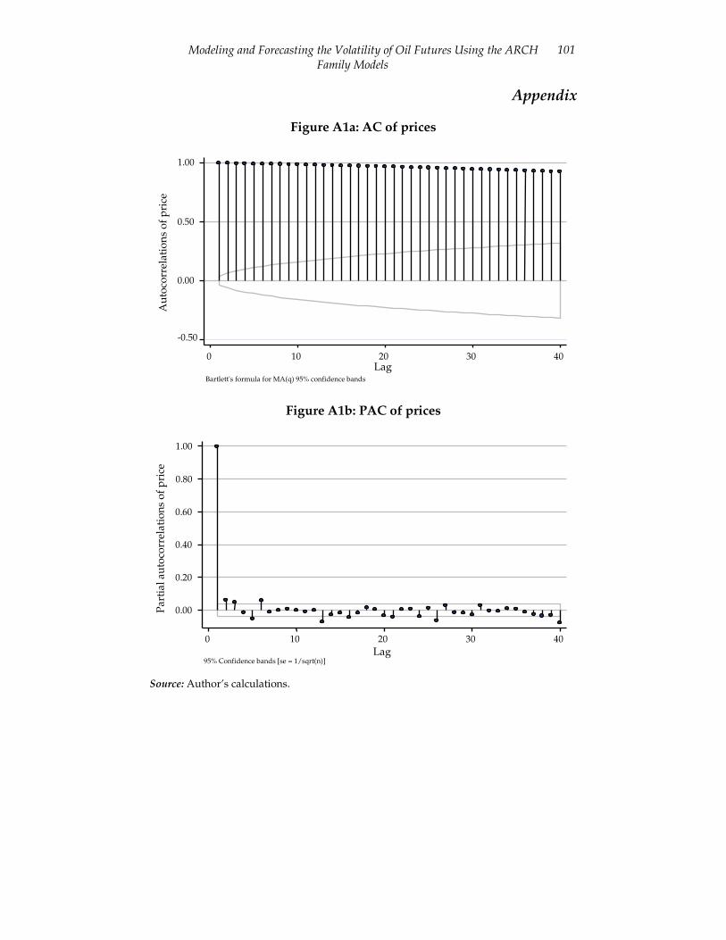
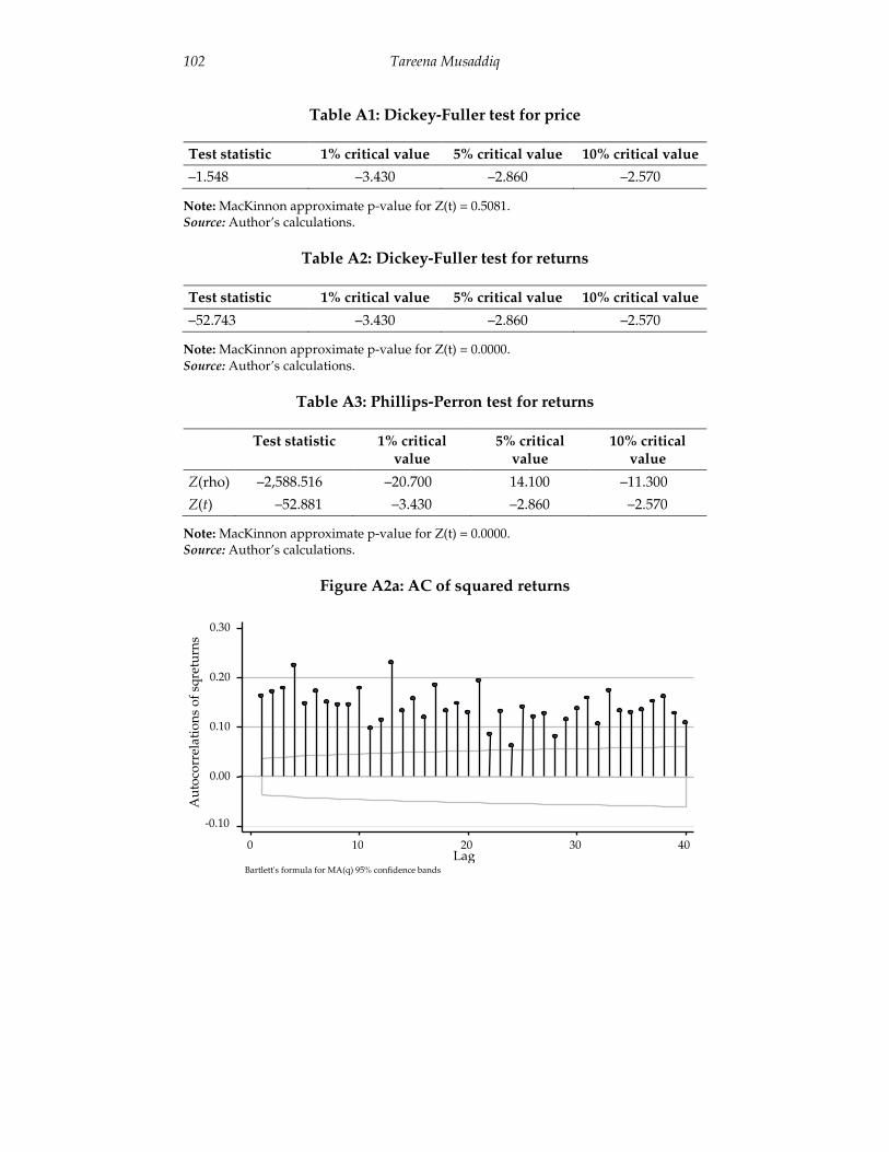
The plotted autocorrelation and partial autocorrelation of the price of the futures contract indicate that the series is nonstationary (Figures A1a and A1b in the Appendix). Applying the Dickey-Fuller test to the series confirms this (Table A1 in the Appendix), and suggests that it cannot be used to model volatility.

Returns rather than prices are more appropriately used here, first, because our aim is to model the volatility of returns on oil futures, and second, because a returns series is more likely to be stationary and thus more suitable for modeling than a price series. The returns are calculated by applying the first difference of the log of prices. Table 1 summarizes the statistics on returns, showing that oil futures have an average daily return of 0.05503 percent and a standard deviation of 0.02616, which indicates an average annualized volatility of 41.53 percent. The skewness coefficient is –0.2203, its sign being common to most financial time series. The kurtosis value is higher than 3, implying that the returns distribution has fat tails. The ARCH family of models should, therefore, be used to account for these characteristics of the data.

2 We have used STATA software to model all specifications by maximum likelihood, and assume the underlying distribution to be normal.


85

Table 1: Summary statistics for returns

Returns

Mean Standard deviation Variance Skewness Kurtosis

0.0005503 0.0261624 0.0006845 –0.2203233 6.805797

Source: Author’s calculations.

It is imperative when modeling such a series that it be stationary and the data mean-reverting. For this purpose, the Dickey-Fuller test is applied to the returns series (Table A2 in the Appendix), and the results show that the series is stationary. On application, the Phillips-Perron test also indicates that the series is stationary and can be used for modeling purposes (Table A3 in the Appendix).

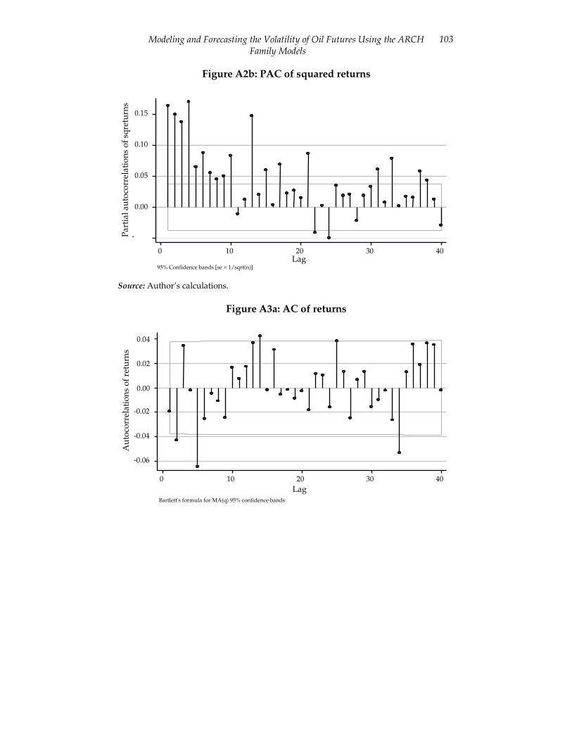
The plotted autocorrelation and partial autocorrelation of squared returns indicate dependence and, hence, imply time-varying volatility (Figures A2a and A2b in the Appendix). This is further supported by the q test for squared returns, which also suggests that is the series is time-dependent.

4. Methodology

In order to model the volatility of the returns, we need to determine their mean equation. The return for today will depend on returns in previous periods (autoregressive component) and the surprise terms in previous periods (moving order component). Plotting the autocorrelation and partial autocorrelation of the returns series can help determine the order of the mean equation.

Like most financial time series, the returns series exhibits what is referred to as “volatility clustering” (Figures A3a and A3b in the Appendix), i.e., it exhibits alternating periods of relative tranquility and unusually large volatility. In order to model such patterns of behavior, the variance of the error term is allowed to depend on its history. The classic model of such behavior is the ARCH model introduced by Engle (1982), which simultaneously models the mean and variance of a series.

For this purpose, if we assume yt to be the returns series and It–1 to be the information set available, then

yt = E[yt It −1]+ε t

86 Tareena Musaddiq

E [.] is the expectations operator and represents the predictable part of the returns, while εt is the unpredictable part and is given by

ε t = yt − βxt

xt is the set of explanatory variables and β is the set of parameters from a linear regression in vector form. The expected value of εt is 0, and its values are serially uncorrelated. Engle (1982) argued that, if we assume that for a time series the forecast of today’s value based on past information is simply E (yt | yt–1), then the forecast for yt depends on the value of the conditioning variable yt–1 and the variance of this one-period forecast is given by (yt | It–1, yt–1). Engel therefore proposed a model under these assumptions in which the variance did depend on past information unlike the conventional models present of the time. The ARCH model simultaneously models the conditional mean and variance of a time series with the conditional heteroscedasticity of the unpredictable part of the series modeled as

ε t = zt ht

ht is a nonnegative function and zt is an i.i.d stochastic process with a zero mean and unit variance. From this, it follows that the conditional mean of εt is 0 and its variance is ht, implying that εt is a heteroscedastic process. Given this information about εt, it can easily be seen that the mean of a series yt, conditional on the past information set is E (yt | It–1) and the variance is ht. Engel proposed the following specification for the process ht:

ht = α0 + α1ε t −12 + α2ε t −2

2 + αqε t −q2 = α0 + α iε t −1

2

i=1

q

∑

αi’ s ≥ 0 and i = 1..., q are constant parameters. This is the so-called ARCH (q) model. As the primary model introduced for modeling volatility, this will be the first model on which we fit our returns series. However, the ARCH model often needs a higher-order q to capture the volatility of a financial time series and, hence, requires estimating many parameters. As Bollerslev (1986) points out, “In empirical applications of the ARCH model a relatively long lag in the conditional variance equation is often called for, and to avoid problems with negative variance parameter estimates a fixed lag structure is typically imposed.” His solution to this problem was the generalized ARCH (GARCH) model,


87

which allows both a more flexible lag structure and a longer memory relative to ARCH specification. As opposed to the ARCH model, the GARCH model’s specification also includes lagged conditional variances. In general, a GARCH (p, q) model is given by

ht = α0 + α iε t − i2

i=1

q

∑ + βiht − ii=1

q

∑

α and β are the parameters to be estimated, p is the number of lags for past variances, and q is the number of lags for past squared residuals. The GARCH model thus allows both autoregressive and moving-average components in heteroscedastic variance. It gives a more parsimonious representation of the ARCH model and is much easier to identify and estimate. The GARCH model is, therefore, the second model that will be fitted to the data.3

Realistically speaking, if “bad news” has a more pronounced effect on volatility than “good news” of the same magnitude, then a symmetric specification such as ARCH or GARCH is not appropriate since in standard ARCH/GARCH models the conditional variance ht is unaffected by the sign of the past periods’ errors (it depends only on squared errors). Various extensions have therefore been proposed to capture these asymmetric effects often shown by financial time series.

Before applying the asymmetric models, however, one needs to test for the presence of such effects. Engle and Ng (1993) propose various tests to detect the presence of asymmetric effects, which are run on the standardized residuals of the GARCH model. The sign bias test is given by

ˆ ε t2 = α0 + α1St −1

− + error

St −1− = 1 when

ˆ ε t −12 < 0, and 0 otherwise. If the dummy variable’s

coefficient is significant and positive, this suggests the presence of asymmetric effects. The negative sign bias test determines whether the size of the negative shock also affects the impact it has on conditional variance, and is given by

ˆ ε t2 = α0 + α1St −1

− + ˆ ε t −1 + error

3 We also estimate the GARCH in the mean form of the GARCH model, which allows the ARCH component in the specification of the mean equation.

88 Tareena Musaddiq

For the existence of a size effect, the coefficient must be negative and significant. The positive sign bias test determines if the size of a positive shock impacts its conditional variance, and is given by

ˆ ε t2 = α0 + α1St −1

+ + ˆ ε t −1 + error

St −1+

St −1− . For the size effect to be present, the coefficient must be

negative and significant. If the tests above indicate the presence of asymmetric effects, then the ARCH/GARCH models are no longer deemed appropriate and their other variants need to be considered.

The first model to account for such effects was the EGARCH model proposed by Nelson (1991). It uses a logarithmic function to treat asymmetric effects, and is given by

Ln(ht ) = α0 + α i |ε t − i

ht − i

−

i=1

q∑ 2π

− γ i

ε t − i

ht − i

i=1

q∑ + βi lni=1

p∑ (ht − i)

In this case, the logarithmic function ensures that the conditional variance is positive and, therefore, the parameters can be allowed to take negative values. The specification implies that the impact of past errors is exponential, unlike standard GARCH models that imply that the effect is quadratic. If the shock is positive, its effect on the log variance is α1 + γ while the effect is α1 – γ if the shock is negative. For significant asymmetric effects, therefore, the coefficient γ should take a negative sign.

Unlike the EGARCH model, Glosten, Jagannathan, and Runkle’s (1993) eponymous model does not look at exponential values but assumes that the impact of squared residuals on the variance depends on whether the residual term is negative or positive. For this purpose, it employs an indicator function as follows:

21

2110 itit

q

i iitq

i ip

i itit Shh −+−=−== − ∑∑∑ +++= εγεαβα

The indicator function

St − i+ takes a value of 1 if εt–i> 0, and 0

otherwise. For the effect of the previous period’s bad news to be greater than the effect of good news of the same magnitude, γshould be significant and have a negative sign.

Zakoïan’s (1994) threshold ARCH (TARCH) model is given by


89

−−

+−== − +++= ∑∑ itiit

q

i ip

i itit hh εγεαβα11

2/10

2/1

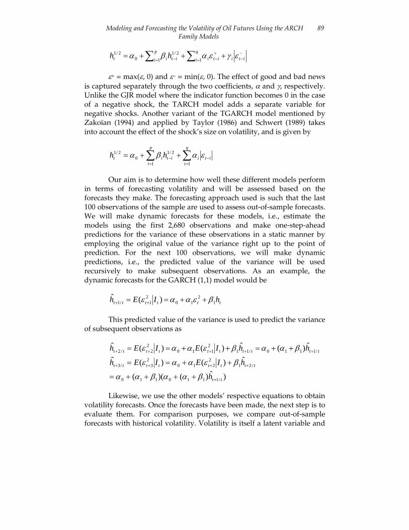
ε+ = max(ε, 0) and ε– = min(ε, 0). The effect of good and bad news is captured separately through the two coefficients, α and γ, respectively. Unlike the GJR model where the indicator function becomes 0 in the case of a negative shock, the TARCH model adds a separate variable for negative shocks. Another variant of the TGARCH model mentioned by Zakoïan (1994) and applied by Taylor (1986) and Schwert (1989) takes into account the effect of the shock’s size on volatility, and is given by

it

q

iiit

p

iit hh −

=−

=∑∑ ++= εαβα

1

2/1

10

2/1

Our aim is to determine how well these different models perform in terms of forecasting volatility and will be assessed based on the forecasts they make. The forecasting approach used is such that the last 100 observations of the sample are used to assess out-of-sample forecasts. We will make dynamic forecasts for these models, i.e., estimate the models using the first 2,680 observations and make one-step-ahead predictions for the variance of these observations in a static manner by employing the original value of the variance right up to the point of prediction. For the next 100 observations, we will make dynamic predictions, i.e., the predicted value of the variance will be used recursively to make subsequent observations. As an example, the dynamic forecasts for the GARCH (1,1) model would be

tttttt hIEh 12

102

1/1 )(ˆ βεααε ++== ++

This predicted value of the variance is used to predict the variance of subsequent observations as

tttttttttt hhIEIEh /1110/112

1102

2/2ˆ)(ˆ)()(ˆ

+++++ ++=++== βααβεααε

tttttttt hIEIEh /212

2102

3/3ˆ)()(ˆ

++++ ++== βεααε

)ˆ)()(( /1110110 tth +++++= βααβαα

Likewise, we use the other models’ respective equations to obtain volatility forecasts. Once the forecasts have been made, the next step is to evaluate them. For comparison purposes, we compare out-of-sample forecasts with historical volatility. Volatility is itself a latent variable and

90 Tareena Musaddiq

thus its value can only be approximated. Previous studies on oil volatility have used daily squared returns from market prices as a proxy (see Agnolucci, 2009; Sadorsky, 2006). Moreover, since the historical volatility figure is used for comparison purposes only, using it as a proxy does not cause problems because it is unbiased (Lopez, 2001).

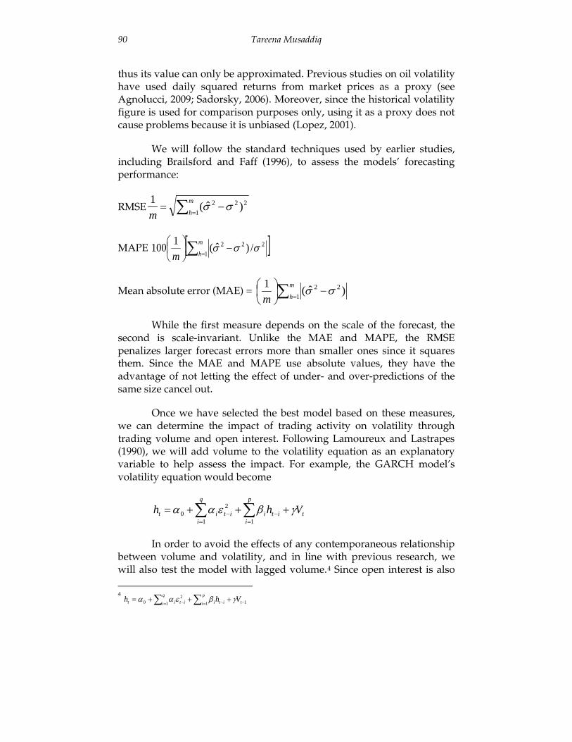
We will follow the standard techniques used by earlier studies, including Brailsford and Faff (1996), to assess the models’ forecasting performance:

RMSE ∑ =−=

m

hm 1222 )ˆ(1 σσ

MAPE [ ]∑ =−

m

hm 1222 /)ˆ(1100 σσσ

Mean absolute error (MAE) = ∑ =−

m

hm 122 )ˆ(1 σσ

While the first measure depends on the scale of the forecast, the second is scale-invariant. Unlike the MAE and MAPE, the RMSE penalizes larger forecast errors more than smaller ones since it squares them. Since the MAE and MAPE use absolute values, they have the advantage of not letting the effect of under- and over-predictions of the same size cancel out.

Once we have selected the best model based on these measures, we can determine the impact of trading activity on volatility through trading volume and open interest. Following Lamoureux and Lastrapes (1990), we will add volume to the volatility equation as an explanatory variable to help assess the impact. For example, the GARCH model’s volatility equation would become

tit

p

iiit

q

iit Vhh γβεαα +++= −

=−

=∑∑

1

2

10

In order to avoid the effects of any contemporaneous relationship between volume and volatility, and in line with previous research, we will also test the model with lagged volume.4 Since open interest is also

4

112

10 −−=−=+++= ∑∑ tit

p

i iitq

i it Vhh γβεαα


91

considered a proxy for trading activity, the model will also be tested with open interest replacing the volume variable. This approach can be generalized for all the models applied to determine whether trading activity reduces volatility persistence and impacts volatility.

Empirical Findings

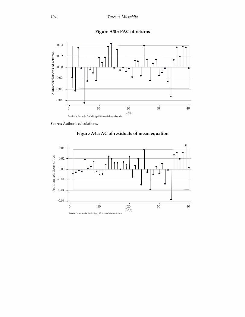
As described in Section 4, our first step is to identify the mean equation for the returns. The autocorrelation and partial autocorrelation function for the returns show that autocorrelations and partial autocorrelations up to the fifth lag are significant (Figures A3a and A3b in the Appendix). We, therefore, propose using an autoregressive moving average (ARMA) (5,5) mean equation to model volatility in the ARCH models. The estimated ARMA (5,5) equation for the mean is found to be significant with a Wald statistic of 799.98 and significant t-values for the coefficients. The residuals of the mean equation indicate the absence of autocorrelation through the q statistic (Figures A4a and A4b in the Appendix). The ARMA (5,5) model is thus deemed an appropriate model for the mean equation.

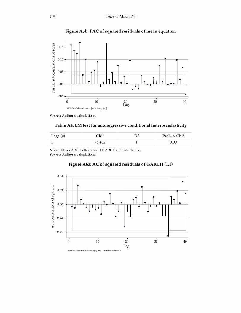
The q statistic implies that there is second-order dependence in the squared residuals of the mean equation and, hence, the presence of conditional heteroscedasticity in the returns (Figures A5a and A5b in the Appendix). Further, the ARCH-Lagrange Multiplier (LM) test gives a Chi-squared value of 75.46, confirming the presence of ARCH effects and the need to model this conditional heteroscedasticity using the ARCH family models (Table A4 in the Appendix).

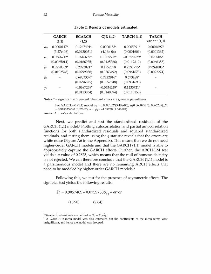
Table 2 presents the results of the models fitted to the data on returns. We do not estimate the ARCH model, the idea being that the GARCH model is a more parsimonious version of higher-order ARCH models. With the ARMA (5,5) as the underlying mean equation, estimating the GARCH (1,1) model reveals that the t-statistics for both coefficients are significant. A value of 0.9251 for past variance implies that the shock of past volatility has a persistent effect on future volatility. The sum of the two coefficients is a succinct measure of the persistence of variance, and that its value is close to 1 implies that there is significant persistence in volatility. The unconditional variance is 0.0006414, which is equivalent to an annualized variance of 10.14 percent.

92 Tareena Musaddiq

Table 2: Results of models estimated

GARCH (1,1)

EGARCH (1,2)

GJR (1,2) TARCH (1,2) TARCH variant (1,1)

α0 0.0000117* (3.27e-06)

0.1267491* (0.0430031)

0.0000153* (4.16e-06)

0.0005391* (0.0001609)

0.0004697* (0.0001362)

α1 0.0566712* (0.0065014)

0.1616697* (0.0166975)

0.1085503* (0.0125366)

–0.0770229* (0.0119319)

0.073906* (0.0066358)

β1 0.9250869* (0.0102548)

0.2922021* (0.0799058)

0.1752578 (0.0863492)

0.2391775* (0.0961673)

0.9241005* (0.0092274)

β2 - 0.6903359* (0.0796525)

0.7222816* (0.0857648)

0.673488* (0.0951695)

-

γ1 - –0.0687259* (0.0113834)

–0.0634249* (0.0148894)

0.1230721* (0.0113155)

-

Notes: * = significant at 5 percent. Standard errors are given in parentheses.

For GARCH-M (1,1) model α0 = 0.0000132*(3.48e-06), α10.0608757*(0.0066205), β1 = 0.9185359*(0.0107267), and β2= –1.59738 (1.546592).


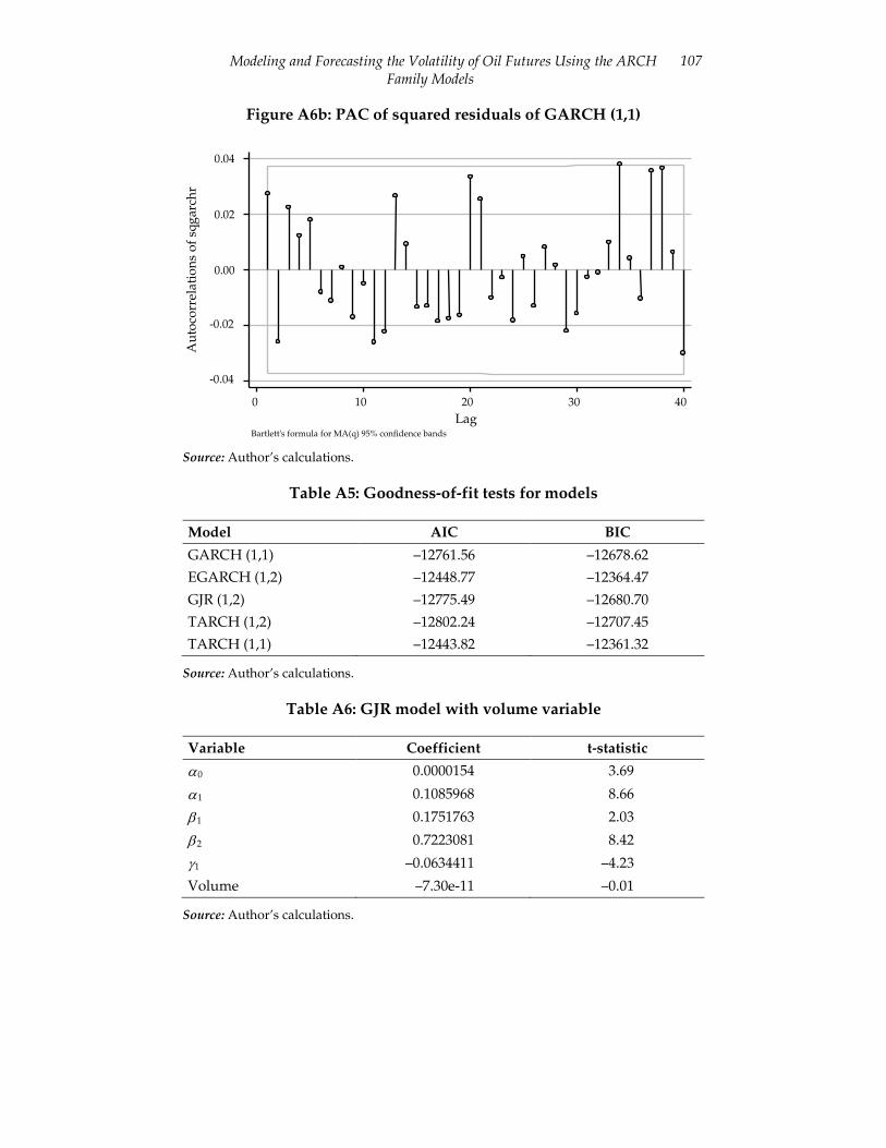
Next, we predict and test the standardized residuals of the GARCH (1,1) model.5 Plotting autocorrelation and partial autocorrelation functions for both standardized residuals and squared standardized residuals, and testing them using the q statistic reveals that the errors are white noise (Figure A6 in the Appendix). This means that we do not need higher-order GARCH models and that the GARCH (1,1) model is able to appropriately capture the GARCH effects. Further, the ARCH-LM test yields a p value of 0.2875, which means that the null of homoscedasticity is not rejected. We can therefore conclude that the GARCH (1,1) model is a parsimonious model and there are no remaining ARCH effects that need to be modeled by higher-order GARCH models.6

Following this, we test for the presence of asymmetric effects. The sign bias test yields the following results:

errorStt ++= −−1

2 0759758.09057469.0ε̂

(16.90) (2.64)

5 Standardized residuals are defined as 𝑆𝑡 = ℰ̂𝑡/ℎ�𝑡. 6 A GARCH-in-mean model was also estimated but the coefficients of the mean terms were insignificant, and hence the model was dropped.


93

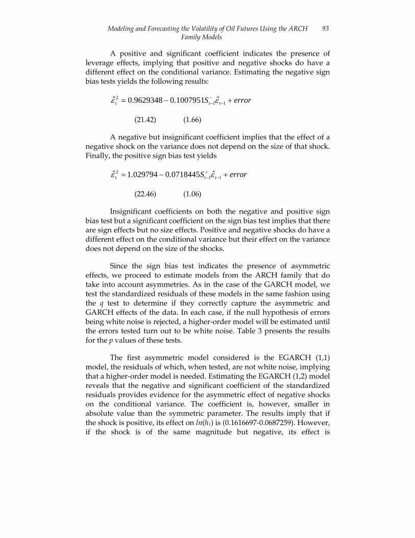
A positive and significant coefficient indicates the presence of leverage effects, implying that positive and negative shocks do have a different effect on the conditional variance. Estimating the negative sign bias tests yields the following results:

errorS ttt +−= −−− 11

2 ˆ1007951.09629348.0ˆ εε

(21.42) (1.66)

A negative but insignificant coefficient implies that the effect of a negative shock on the variance does not depend on the size of that shock. Finally, the positive sign bias test yields

errorS ttt +−= −+− 11

2 ˆ0718445.0029794.1ˆ εε

(22.46) (1.06)

Insignificant coefficients on both the negative and positive sign bias test but a significant coefficient on the sign bias test implies that there are sign effects but no size effects. Positive and negative shocks do have a different effect on the conditional variance but their effect on the variance does not depend on the size of the shocks.

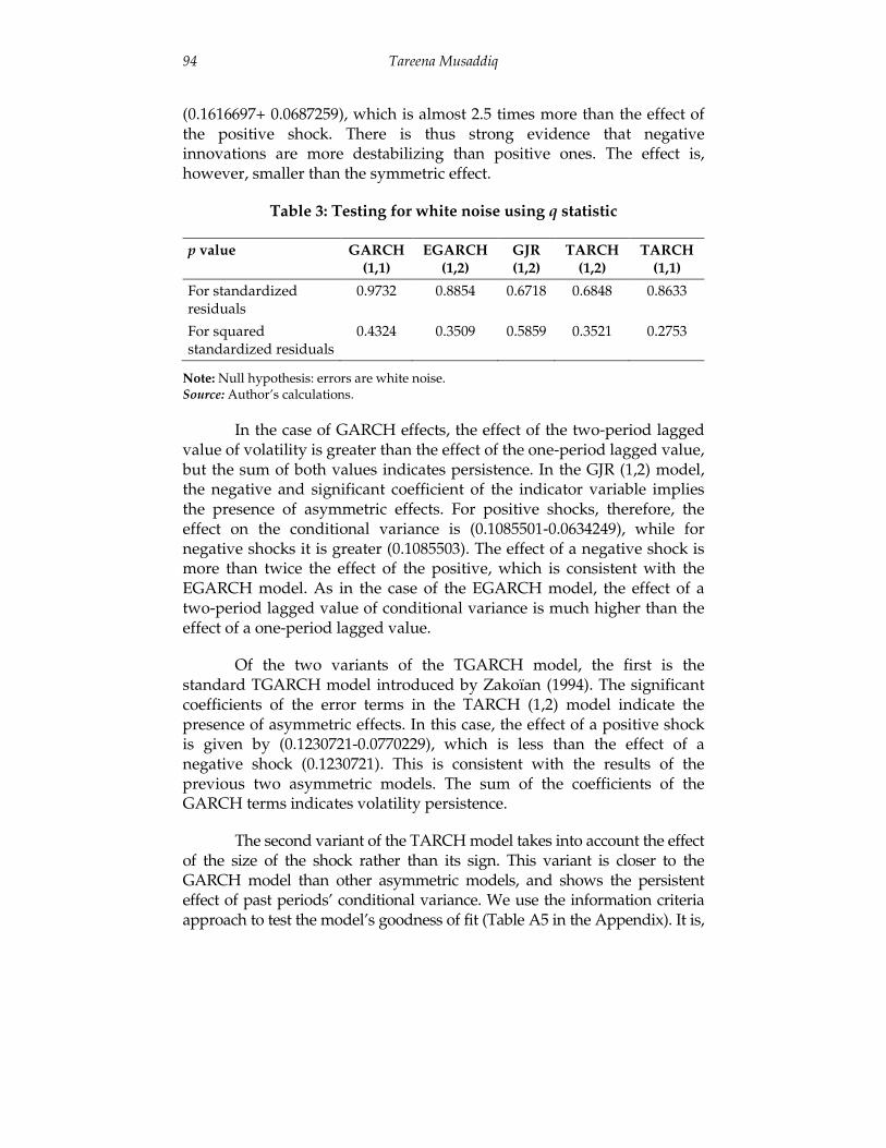
Since the sign bias test indicates the presence of asymmetric effects, we proceed to estimate models from the ARCH family that do take into account asymmetries. As in the case of the GARCH model, we test the standardized residuals of these models in the same fashion using the q test to determine if they correctly capture the asymmetric and GARCH effects of the data. In each case, if the null hypothesis of errors being white noise is rejected, a higher-order model will be estimated until the errors tested turn out to be white noise. Table 3 presents the results for the p values of these tests.

The first asymmetric model considered is the EGARCH (1,1) model, the residuals of which, when tested, are not white noise, implying that a higher-order model is needed. Estimating the EGARCH (1,2) model reveals that the negative and significant coefficient of the standardized residuals provides evidence for the asymmetric effect of negative shocks on the conditional variance. The coefficient is, however, smaller in absolute value than the symmetric parameter. The results imply that if the shock is positive, its effect on ln(ht) is (0.1616697-0.0687259). However, if the shock is of the same magnitude but negative, its effect is

94 Tareena Musaddiq

(0.1616697+ 0.0687259), which is almost 2.5 times more than the effect of the positive shock. There is thus strong evidence that negative innovations are more destabilizing than positive ones. The effect is, however, smaller than the symmetric effect.

Table 3: Testing for white noise using q statistic

p value GARCH (1,1)

EGARCH (1,2)

GJR (1,2)

TARCH (1,2)

TARCH (1,1)

For standardized residuals

0.9732 0.8854 0.6718 0.6848 0.8633

For squared standardized residuals

0.4324 0.3509 0.5859 0.3521 0.2753

Note: Null hypothesis: errors are white noise. Source: Author’s calculations.

In the case of GARCH effects, the effect of the two-period lagged value of volatility is greater than the effect of the one-period lagged value, but the sum of both values indicates persistence. In the GJR (1,2) model, the negative and significant coefficient of the indicator variable implies the presence of asymmetric effects. For positive shocks, therefore, the effect on the conditional variance is (0.1085501-0.0634249), while for negative shocks it is greater (0.1085503). The effect of a negative shock is more than twice the effect of the positive, which is consistent with the EGARCH model. As in the case of the EGARCH model, the effect of a two-period lagged value of conditional variance is much higher than the effect of a one-period lagged value.

Of the two variants of the TGARCH model, the first is the standard TGARCH model introduced by Zakoïan (1994). The significant coefficients of the error terms in the TARCH (1,2) model indicate the presence of asymmetric effects. In this case, the effect of a positive shock is given by (0.1230721-0.0770229), which is less than the effect of a negative shock (0.1230721). This is consistent with the results of the previous two asymmetric models. The sum of the coefficients of the GARCH terms indicates volatility persistence.

The second variant of the TARCH model takes into account the effect of the size of the shock rather than its sign. This variant is closer to the GARCH model than other asymmetric models, and shows the persistent effect of past periods’ conditional variance. We use the information criteria approach to test the model’s goodness of fit (Table A5 in the Appendix). It is,


95

however, important to note that our main aim is to evaluate forecasts and, hence, forecast evaluation measures better serve this purpose.7

Although all asymmetric extensions of the GARCH model use different techniques to capture volatility, they produce consistent results for crude oil futures traded at the NYMEX, and imply the presence of asymmetric effects. This is in contrast to the findings of Agnolucci (2009) and Sadorsky (2006), and may be because the time frame we have used is different from the latter two, which employ data only up to 2005 and so do not take into account the recent financial crisis. Moreover, Agnolucci’s (2009) asymmetric models do not consider higher-order GARCH effects, while previous research does not take into account some of the variants we have used here.

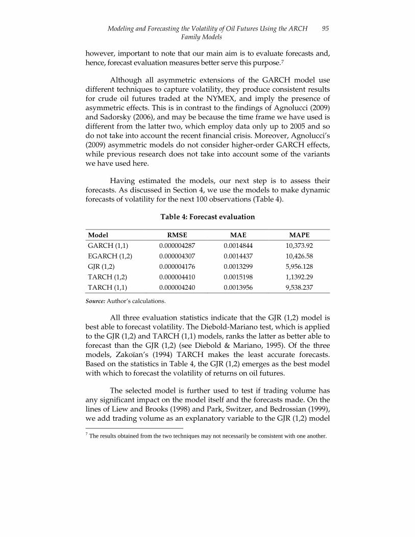
Having estimated the models, our next step is to assess their forecasts. As discussed in Section 4, we use the models to make dynamic forecasts of volatility for the next 100 observations (Table 4).

Table 4: Forecast evaluation

Model RMSE MAE MAPE

GARCH (1,1) 0.000004287 0.0014844 10,373.92

EGARCH (1,2) 0.000004307 0.0014437 10,426.58

GJR (1,2) 0.000004176 0.0013299 5,956.128

TARCH (1,2) 0.000004410 0.0015198 1,1392.29

TARCH (1,1) 0.000004240 0.0013956 9,538.237


All three evaluation statistics indicate that the GJR (1,2) model is best able to forecast volatility. The Diebold-Mariano test, which is applied to the GJR (1,2) and TARCH (1,1) models, ranks the latter as better able to forecast than the GJR (1,2) (see Diebold & Mariano, 1995). Of the three models, Zakoïan’s (1994) TARCH makes the least accurate forecasts. Based on the statistics in Table 4, the GJR (1,2) emerges as the best model with which to forecast the volatility of returns on oil futures.

The selected model is further used to test if trading volume has any significant impact on the model itself and the forecasts made. On the lines of Liew and Brooks (1998) and Park, Switzer, and Bedrossian (1999), we add trading volume as an explanatory variable to the GJR (1,2) model 7 The results obtained from the two techniques may not necessarily be consistent with one another.

96 Tareena Musaddiq

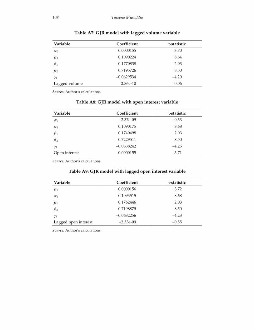
(Table A6 in the Appendix). The coefficient of the volume variable is insignificant, indicating that volume does not have any significant impact on estimation and forecasting through the GJR model. The same is the case when using the lagged value of volume (Table A7 in the Appendix). This result is consistent with the findings of Foster (1995) but updates the latter’s research by using data up to 2009, and concludes that volume does not reduce persistence in crude oil futures.

Another measure of trading activity is open interest (Bessembinder & Seguin, 1993), which we use as a proxy and test using the GJR model. As with volume, its coefficient is insignificant, indicating that open interest does not impact the estimation of volatility modeling (Tables A8 and A9 in the Appendix).

6. Conclusion

This study has attempted to model the volatility of crude oil futures and assess the forecasting ability of the ARCH family of models. We have used historical volatility for modeling purposes through the ARCH family of models and made dynamic forecasts of future volatility. The study finds the presence of asymmetric effects in the light, sweet, crude oil futures traded on the NYMEX. Of the ARCH models, the GJR (1,2) is able to make the most accurate forecasts with the TARCH (1,1) as a close second. Therefore, when volatility forecasts for oil futures are used for hedging and pricing purposes, asymmetric rather than symmetric models are best used. Additionally, we find that trading volume and open interest are unable to reduce volatility persistence in these futures.

The models’ forecasts can be extended for use in asset pricing models. Further improvements to the current study are also possible. First, intraday data and realized volatility could prove a better proxy for actual volatility than squared residuals. This would refine the process of forecast evaluation. Second, asymmetric power models and fractionally integrated models—also of the ARCH family—could be used to analyze volatility behavior.


97

References

Agnolucci, P. (2009). Volatility in crude oil futures: A comparison of the predictive ability of GARCH and implied volatility models. Energy Economics, 31, 316–321.

Alsubaie, A., & Najand, M. (2009). Trading volume, time-varying conditional volatility, and asymmetric volatility spillover in the Saudi stock market. Journal of Multinational Financial Management, 19, 139–149.

Bessembinder, H., & Seguin, P. J. (1993). Price volatility, trading volume and market depth: Evidence from futures markets. Journal of Financial and Quantitative Analysis, 28, 21–39.

Bollerslev, T. (1986). Generalized autoregressive conditional heteroscedasticity. Journal of Econometrics, 31, 307–327.

Bollerslev, T., Chou, R., & Kroner, K. F. (1992). ARCH modeling in finance: A review of the theory and empirical evidence. Journal of Econometrics, 52, 5–59.

Bracker, K., & Smith, K. L. (1999). Detecting and modeling volatility in the copper futures market. Journal of Futures Markets, 19(1), 79–100.

Brailsford, T. J. (1996). The empirical relationship between trading volume, returns, and volatility. Accounting and Finance, 35, 89–111.

Brailsfold, T. J., & Faff, R. W. (1996). An evaluation of volatility forecasting techniques. Journal of Banking and Finance, 20, 419–438.

Brooks, C. (1998). Predicting stock index volatility: Can market volume help? Journal of Forecasting, 17, 59–80.

Brooks, C., & Persand, G. (2003). Volatility forecasting for risk management. Journal of Forecasting, 22, 1–22.

Carvalho, A. F., da Costa, J. S., & Lopes, J. A. (2006). A systematic modeling strategy for futures markets volatility. Applied Financial Economics, 16, 819–833.

Clark, P. K. (1973). A subordinated stochastic process model with finite variance for speculative prices. Econometrica, 41, 135–156.

98 Tareena Musaddiq

Darrat, A. F., Rahman, S., & Zhong, M. (2003). Intraday trading volume and return volatility of the DJIA stocks: A note. Journal of Banking and Finance, 27, 2035–2043.

Dickey, D., & Fuller, W. (1979). Distributions of the estimators for autoregressive time series with a unit root. Journal of the American Statistical Association, 74, 427–431.

Diebold, F., & Mariano, R. (1995). Comparing predictive accuracy. Journal of Business and Economic Statistics, 13(3), 253–263.

Engle, R. F. (1982). Autoregressive conditional heteroscedasticity with estimates of the variance of United Kingdom inflation. Econometrica, 50, 987–1007.

Engle, R. F., & Ng, V. K. (1993). Measuring and testing the impact of news on volatility. Journal of Finance, 48, 1749–1778.

Ferderer, J. (1996). Oil price volatility and the macro-economy. Journal of Macroeconomics, 18, 1–26.

Foster, A. J. (1995). Volume volatility relationships for crude oil futures market. Journal of Futures Markets, 15, 929–951.

Gallo, G. M., & Pacini, B. (2000). The effects of trading activity on market volatility. European Journal of Finance, 6, 163–175.

Glosten, L. R., Jagannathan, R., & Runkle, D. E. (1993). On the relation between the expected value and the volatility of the nominal excess return on stock. Journal of Finance, 48, 1779–1801.

Hull, J. C. (2005). Options futures and other derivatives (6th ed.). Upper Saddle River, NJ: Prentice Hall.

Kang, S.-H., Kang, S.-M., & Yoon, S.-M. (2009). Forecasting volatility of crude oil markets. Energy Economics, 31, 119–125.

Lamoureux, G. C., & Lastrapes, W. D. (1990). Heteroscedasticity in stock return data: Volume versus GARCH effects. Journal of Finance, 45, 221–229.

Lee, K., Ni, S., & Rutti, R. A. (1995). Oil shocks and the macro-economy: The role of price variability. The Energy Journal, 16, 39–56.


99

Liew, K. Y., & Brooks, R. (1998). Returns and volatility in the Kuala Lumpur crude palm oil futures market. Journal of Futures Markets, 18, 985–999.

Lopez, J. A. (2001). Evaluating the predictive accuracy of volatility models. Journal of Forecasting, 20, 87–109.

Najand, M., & Yung, K. (1991). A GARCH examination of the relationship between volume and price variability in futures market. Journal of Futures Markets, 11, 613–621.

Nelson, D. B. (1991). Conditional heteroscedasticity in asset returns: A new approach. Econometrica, 59, 347–370.

Pagan, A. R., & Schwert, G. W. (1990). Alternative models for conditional stock volatility. Journal of Econometrics, 45, 267–290.

Park, T.-H, Switzer, L. N., & Bedrossian, R. (1999). The interactions between trading volume and volatility: Evidence from the equity options market. Applied Financial Economics, 9, 627–637.

Phillips, P. C. B., & Perron, P. (1988). Testing for a unit root in time series regression. Biometrika, 75, 335–346.

Poon, S.-H., & Granger, C. W. J. (2003). Forecasting volatility in financial markets: A review. Journal of Economic Literature, 41, 478–539.

Pyuna, C. S., Lee, S. Y., & Nam, K. (2000). Volatility and information flows in emerging equity markets: A case of the Korean Stock Exchange. International Review of Financial Analysis, 9, 405–420.

Ragunathan, V., & Peker, A. (1997). Price variability, trading volume and market depth: Evidence from the Australian futures market. Applied Financial Economics, 7, 447–454.

Sadorsky, P. (1999). Oil price shocks and stock market activity. Energy Economics, 21, 449–469.

Sadorsky, P. (2006). Modeling and forecasting petroleum futures volatility. Energy Economics, 28, 467–488.

Schwert, G. W. (1989). Why does stock market volatility change over time? Journal of Finance, 44(5), 1115–1153.

100 Tareena Musaddiq

Schwert, G. W. (1990). Stock volatility and the crash of ’87. Review of Financial Studies, 3, 77–102.

Sharma, J. L., Mougous, M., & Kamath, R. (1996). Heteroscedasticity in stock market indicator return data: Volume versus GARCH effects. Applied Financial Economics, 6, 337–342.

Taylor, S. (1986). Modeling financial time series. Chichester, UK: Wiley.

Zakoïan, J.-M. (1994). Threshold heteroscedastic models. Journal of Economic Dynamics and Control, 18, 931–955.


101

Appendix

Figure A1a: AC of prices

Figure A1b: PAC of prices


0.00

0.20

0.40

0.60

0.80

1.00

Part

ial a

utoc

orre

lati

ons

of p

rice

0 10 20 30 40 Lag

95% Confidence bands [se = 1/sqrt(n)]

-0.50

0.00

0.50

1.00

0 10 20 30 40 Lag

Bartlett's formula for MA(q) 95% confidence bands

Aut

ocor

rela

tion

s of

pri

ce


Table A1: Dickey-Fuller test for price

Test statistic 1% critical value 5% critical value 10% critical value

–1.548 –3.430 –2.860 –2.570

Note: MacKinnon approximate p-value for Z(t) = 0.5081. Source: Author’s calculations.

Table A2: Dickey-Fuller test for returns

Test statistic 1% critical value 5% critical value 10% critical value

–52.743 –3.430 –2.860 –2.570


Table A3: Phillips-Perron test for returns

Test statistic 1% critical value

5% critical value

10% critical value

Z(rho) –2,588.516 –20.700 14.100 –11.300

Z(t) –52.881 –3.430 –2.860 –2.570


Figure A2a: AC of squared returns

-0.10

0.00

0.10

0.20

0.30

0 10 20 30 40 Lag


Aut

ocor

rela

tion

s of

sqr

etur

ns


103

Figure A2b: PAC of squared returns


Figure A3a: AC of returns

-0.06

-0.04

-0.02

0.00

0.02

0.04

Aut

ocor

rela

tion

s of

ret

urns

0 10 20 30 40 Lag


-

0.00

0.05

0.10

0.15

Part

ial a

utoc

orre

lati

ons

of s

qret

urns

0 10 20 30 40 Lag



Figure A3b: PAC of returns


Figure A4a: AC of residuals of mean equation

-0.06

-0.04

-0.02

0.00

0.02

0.04

Aut

ocor

rela

tion

s of

res

0 10 20 30 40 Lag


-0.06

-0.04

-0.02

0.00

0.02

0.04

Aut

ocor

rela

tion

s of

ret

urns

0 10 20 30 40 Lag



105

Figure A4b: PAC of residuals of mean equation


Figure A5a: AC of squared residuals of mean equation

-0.05

0.00

0.05

0.10

0.15

0.20

Aut

ocor

rela

tion

s of

sqr

es

0 10 20 30 40 Lag


-0.06

-0.04

-0.02

0.00

0.02

0.04

Part

ial a

utoc

orre

lati

ons

of r

es

0 10 20 30 40 Lag



Figure A5b: PAC of squared residuals of mean equation


Table A4: LM test for autoregressive conditional heteroscedasticity

Lags (p) Chi2 Df Prob. > Chi2

1 75.462 1 0.00

Note: H0: no ARCH effects vs. H1: ARCH (p) disturbance. Source: Author’s calculations.

Figure A6a: AC of squared residuals of GARCH (1,1)

-0.04

-0.02

0.00

0.02

0.04

Aut

ocor

rela

tion

s of

sga

rchr

0 10 20 30 40 Lag


-0.05

0.00

0.05

0.10

0.15

Part

ial a

utoc

orre

lati

ons

of s

qres

0 10 20 30 40 Lag



107

Figure A6b: PAC of squared residuals of GARCH (1,1)


Table A5: Goodness-of-fit tests for models

Model AIC BIC

GARCH (1,1) –12761.56 –12678.62

EGARCH (1,2) –12448.77 –12364.47

GJR (1,2) –12775.49 –12680.70

TARCH (1,2) –12802.24 –12707.45

TARCH (1,1) –12443.82 –12361.32


Table A6: GJR model with volume variable

Variable Coefficient t-statistic

α0 0.0000154 3.69

α1 0.1085968 8.66

β1 0.1751763 2.03

β2 0.7223081 8.42

γ1 –0.0634411 –4.23

Volume –7.30e-11 –0.01


-0.04

-0.02

0.00

0.02

0.04

Aut

ocor

rela

tion

s of

sqg

arch

r

0 10 20 30 40 Lag



Table A7: GJR model with lagged volume variable


α0 0.0000155 3.70

α1 0.1090224 8.64

β1 0.1770838 2.03

β2 0.7195726 8.30

γ1 –0.0629534 –4.20

Lagged volume 2.86e-10 0.06


Table A8: GJR model with open interest variable


α0 –2.37e-09 –0.53

α1 0.1090175 8.68

β1 0.1740498 2.03

β2 0.7229511 8.50

γ1 –0.0638242 –4.25

Open interest 0.0000155 3.71


Table A9: GJR model with lagged open interest variable


α0 0.0000156 3.72

α1 0.1093515 8.68

β1 0.1762446 2.03

β2 0.7198879 8.50

γ1 –0.0632256 –4.23

Lagged open interest –2.53e-09 –0.55


Modeling and Forecasting the Volatility of Oil Futures Using the ARCH ... · PDF fileModeling...

Documents

Transcript of Modeling and Forecasting the Volatility of Oil Futures Using the ARCH ... · PDF fileModeling...