Modeling and Experiments of Buckling Modes and Deflection ...

Gregory L. Holste-mail: [email protected]

Gregory H. Teicherte-mail: [email protected]

Brian D. Jensen1

e-mail: [email protected]

Department of Mechanical Engineering,

Brigham Young University,

Provo, Utah 84602

Modeling and Experiments ofBuckling Modes and Deflectionof Fixed-Guided Beams inCompliant MechanismsThis paper explores the deflection and buckling of fixed-guided beams used in compliantmechanisms. The paper’s main contributions include the addition of an axial deflectionmodel to existing beam bending models, the exploration of the deflection domain of afixed-guided beam, and the demonstration that nonlinear finite element models typicallyincorrectly predict a beam’s buckling mode unless unrealistic constraints are placed onthe beam. It uses an analytical model for predicting the reaction forces, moments, andbuckling modes of a fixed-guided beam undergoing large deflections. The model for thebending behavior of the beam is found using elliptic integrals. A model for the axialdeflection of the buckling beam is also developed. These two models are combined to pre-dict the performance of a beam undergoing large deflections including higher orderbuckling modes. The force versus displacement predictions of the model are compared tothe experimental force versus deflection data of a bistable mechanism and a thermome-chanical in-plane microactuator (TIM). The combined models show good agreement withthe force versus deflection data for each device. [DOI: 10.1115/1.4003922]

1 Introduction

Compliant mechanisms are kinematic mechanisms whosemotion is derived from the deflection of flexible members ratherthan rotation of pin joints with rigid links. Compliant mechanismshave been used to replace rigid body mechanisms to reduce theircost and to improve their performance due to lower part counts,increased precision, and reduced wear [1]. One example of theeffective use of compliant mechanisms is in microelectromechani-cal systems (MEMS) [2–4].

There are several modeling techniques used to predict the per-formance of these mechanisms, including the pseudo rigid bodymodel (PRBM) [1,5], elastic beam bending solutions [6–8], ellip-tic integral solutions [1,9–12], and finite element models [13–15].These have provided an increased insight into the behavior ofcompliant mechanisms by predicting the reaction forces andmoments for different arrangements of flexible beams.

This paper will focus on the modeling of fixed-guided beamsused in compliant mechanisms such as bistable mechanisms andthermomechanical microactuators [5,6,11,13,16,17].

The PRBM accurately predicts the motion of fixed-guided beamsbut is limited to first mode bending in its accuracy [8]. Nonlinear fi-nite element models can predict higher-order modes of buckling,but they often predict the wrong buckling mode (third or higherinstead of the more realistic second mode seen in practice). To cor-rect this error, an offset force has been applied to bias the bucklingof the thin beam [13]. The biasing force corrects the buckling modebut can add an unrealistic loading condition to the model. In thispaper, we utilize an elliptic integral model for a beam with a fixed-guided end condition derived from the general solution in Ref. [9].A similar derivation by Zhao et al. [18] uses a numerical approxi-mation instead of elliptic integrals for the fixed-guided configura-tion. This paper also adds a model of axial beam deflections tomore accurately predict the onset of buckling. The model presented

here predicts the motion of a fixed-guided beam in both first, sec-ond, and higher bending modes and is capable of accurately pre-dicting which mode corresponds to a given beam end displacement.A novel contribution of this paper is the insight gained into buck-ling behavior of fixed-guided beams as a function of end displace-ment. The behavior over a wide range of deflections is explored,rather than limiting deflection to a single line as been done in thepast [18]. This shows the determination of zones of deflection lead-ing to first or second mode bending. This paper concludes by com-paring the force versus deflection data predicted by the model withexperimental data from a bistable mechanism and a thermomechan-ical microactuator, demonstrating the accuracy of the model.

2 Model

The model developed here to predict the reaction forces anddisplacements of a flexible beam is made up of two parts. The firstis a lateral bending model that accounts for the bending behaviorof the beam, and an axial deflection model to account for theforces being transmitted through the beam. The bending modelcalculates the reaction forces due to bending and these are appliedto the axial deflection model to find the displacements due to axialstretching or compression.

2.1 Bending Model Derivation. The bending model devel-oped here presents an analytical solution for the higher orderbending modes for a beam with fixed-guided end conditions. Themodel assumes a constant second moment of area, a constantmodulus of elasticity, and an inextensible beam. The equations forthe lateral bending model derive from the Bernoulli Euler beamtheory which states that the moment in the beam is proportional tothe curvature. The Bernoulli Euler equation for the moment in thebeam at point A in Fig. 1 is

EIdhds¼ M1 � RðxaÞ sin wþ RðyaÞ cos w (1)

where ya and xa are the vertical and horizontal coordinates ofpoint A, respectively and M, R, and w are defined in the figure.For a coordinate s along the beam’s length,

1Corresponding author.Contributed by the Design Innovation and Devices Committee of ASME for

publication in the JOURNAL OF MECHANICAL DESIGN. Manuscript received December22, 2010; final manuscript received March 30, 2011; published online June 2, 2011.Assoc. Editor: Alexander Slocum.

Journal of Mechanical Design MAY 2011, Vol. 133 / 051002-1Copyright VC 2011 by ASME

Downloaded From: http://mechanicaldesign.asmedigitalcollection.asme.org/ on 01/12/2015 Terms of Use: http://asme.org/terms

dya

ds¼ sin h (2)

dxa

ds¼ cos h (3)

Differentiating Eq. (1) with respect to s gives

EId2hds2¼ �R cos h sin wþ R sin h cos w (4)

Integrating Eq. (4) with respect to h results in

EI

2

dhds

� �2

¼ �R sin h sin w� R cos h cos wþ C (5)

Solving for ds in Eq. (5) and substituting into

L ¼ðL

0

ds (6)

bb ¼ðL

0

sin hds (7)

ab ¼ðL

0

cos hds (8)

gives the integrals for the displacements

L ¼ðL

0

ffiffiffiffiffiEIpffiffiffiffiffiffiffiffiffiffiffiffiffiffiffiffiffiffiffiffiffiffiffiffiffiffiffiffiffiffiffiffiffiffiffiffiffiffiffiffiffiffiffi

�2R cosðh� wÞ þ 2Cp dh (9)

bb ¼ðL

0

ffiffiffiffiffiEIp

sin hffiffiffiffiffiffiffiffiffiffiffiffiffiffiffiffiffiffiffiffiffiffiffiffiffiffiffiffiffiffiffiffiffiffiffiffiffiffiffiffiffiffiffi�2R cosðh� wÞ þ 2C

p dh (10)

ab ¼ðL

0

ffiffiffiffiffiEIp

cos hffiffiffiffiffiffiffiffiffiffiffiffiffiffiffiffiffiffiffiffiffiffiffiffiffiffiffiffiffiffiffiffiffiffiffiffiffiffiffiffiffiffiffi�2R cosðh� wÞ þ 2C

p dh (11)

where bb and ab are the vertical and horizontal displacements ofthe beam due to bending. Equation (6) assumes an inextensiblebeam. To evaluate these integrals, we define k such that

C ¼ Rð2k2 � 1Þ (12)

and introduce another variable / such that

cosw� h

2

� �¼ k sin / (13)

Manipulating Eq. (13) with trigonometric identities gives

cosðh� wÞ ¼ 2k2 sin2 /� 1 (14)

Differentiating with respect to / gives

� sinðw� hÞ dhd/¼ 4k2 cos / sin / (15)

which can be manipulated by substituting Eq. (13) and using trig-onometric identities to obtain

dh ¼ d/2k cos /ffiffiffiffiffiffiffiffiffiffiffiffiffiffiffiffiffiffiffiffiffiffiffiffiffi

1� k2 sin2 /p

!(16)

Substituting Eqs. (12), (14), and (16) into Eq. (9) gives

L ¼ð/2

/1

ffiffiffiffiffiEI

R

rd/ffiffiffiffiffiffiffiffiffiffiffiffiffiffiffiffiffiffiffiffiffiffiffiffiffi

1� k2 sin2 /p (17)

and defining a constant, a, to be

a ¼ L2R

EI(18)

and using the definition of the incomplete elliptic integral of thefirst kind, Fðk;/Þ

Fðk;/Þ ¼ð/

0

ddffiffiffiffiffiffiffiffiffiffiffiffiffiffiffiffiffiffiffiffiffiffiffi1� k2 sin dp (19)

reduces Eq. (17) to ffiffiffiap¼ Fðk;/2Þ � Fðk;/1Þ (20)

/1 and /2 are discussed below. a is the non-dimensional reactionforce.

Next, we use trigonometric identities and Eq. (13) to manipu-late sin h to the correct form to find the vertical end displacementof the beam, bb.

sin h ¼ sinðh� wÞ cos wþ cosðh� wÞ sin w (21)

sin h ¼ �2k cos w sin /ð1� k2 sin2 /Þ12

þ sin wð2k2 sin2 /� 1Þ (22)

By substituting the result into Eq. (10) and following the samesubstitutions used to find Eq. (20), elliptic integrals can then beused to solve for bb.

Again, we use trigonometric identities and Eq. (13) to manipu-late cos h to the correct form to find the vertical end displacementof the beam, ab.

cos h ¼ cosðh� wÞ cos w� sinðh� wÞ sin w (23)

cos h ¼ 2k sin w sin /ð1� k2 sin2 wÞ12 þ cos wð2k2 sin /� 1Þ

(24)

By substituting the result into Eq. (11) and following thesame substitutions used to find Eq. (20), elliptic integrals can thenbe used to solve for ab. The equations for the end displacementsare

bb

L¼ �1ffiffiffi

ap fsin w½2Eðk;/2Þ � 2Eðk;/1Þ � 2Fðk;/2Þ þ 2Fðk;/1Þ�

þ 2k cos wðcos /1 � cos /2Þg (25)

ab

L¼ �1ffiffiffi

ap fcos w½2Eðk;/2Þ � 2Eðk;/1Þ � 2Fðk;/2Þ þ 2Fðk;/1Þ�

þ 2k cos wðcos /2 � cos /1Þg (26)

Fig. 1 Diagram of variables used for the fixed-guided bucklingbeam solution

051002-2 / Vol. 133, MAY 2011 Transactions of the ASME


where the nondimensional displacements bb=L and ab=L are thevertical and horizontal displacements, respectively. Fðk;/Þ is theincomplete elliptic integral of the first kind with an amplitude of/ and a modulus of k defined above, and Eðk;/Þ is the incompleteelliptic integral of the second kind, again with an amplitude of /and a modulus of k defined as

Eðk;/Þ ¼ð/

0

ffiffiffiffiffiffiffiffiffiffiffiffiffiffiffiffiffiffiffiffiffiffiffiffi1� k2 sin2 d

p� �dd (27)

For more information on the use and derivation of elliptic inte-grals, see Refs. [19,20].

In addition to the prediction model for the reaction force andend displacements, the displaced shape of the buckled beams canbe found using

yi

L¼ �1ffiffiffi

ap fsin w½2Eðk;/iÞ � 2Eðk;/1Þ þ Fðk;/1Þg � Fðk;/iÞ�

þ 2k cos wðcos /1 � cos /iÞ (28)

xi

L¼ �1ffiffiffi

ap fcos w½2Eðk;/iÞ � 2Eðk;/1Þ þ Fðk;/1Þg � Fðk;/iÞ�

þ 2k sin wðcos /i � cos /1Þ (29)

where xi and yi are the coordinates of the profile of the beam cor-responding to a value of /i, which ranges from /1 to /2.

The nondimensional reaction moments at the ends of the beam,b1 and b2, are derived from the Bernouli-Euler equation at theends of the beam where

M ¼ EIdhds

(30)

Substituting from Eqs. (5) and (12) gives

b1 ¼M1L

EI¼ 2k

ffiffiffiap

cos /1 (31)

b2 ¼M2L

EI¼ 2k

ffiffiffiap

cos /2 (32)

where /1 and /2 are associated with the origin and displaced endof the beam, respectively, as shown in Fig. 2. The variable /1 canbe calculated using

sin /1 ¼1

kcos

w2

� �(33)

The physical significance of the variables k and / is not readilyapparent but the behavior of this system gives some insight into

their meaning. For example, / is a variable whose value changescontinuously from /1 at the left end of the beam to /2 at the rightend. The inflection points of the beam occur when / is equal to anodd multiple of p=2 such as p=2, 3p=2, 5p=2, etc. as illustrated inFig. 2.

For fixed-guided boundary conditions, the variable /1 can berelated to /2 by the following equation

sin /1 ¼ sin /2 (34)

which has an infinite set of solutions for /2 for any given /1. Todetermine the value of /2 for a given /1, the solutions of Eq. (34)are

/2 ¼ np� /1 if n is odd (35)

/2 ¼ npþ /1 if n is even (36)

and n is the mode of bending predicted. Because the inflectionpoints occur at odd multiples of p

2, the mode number corresponds

to the number of inflection points in the deflected beam shape.Third order, ðn ¼ 3Þ, and higher bending modes occur in idealcases but are not encountered in most real systems due to slightasymmetries of the mechanism or due to asymmetric reactionforces and moments. Therefore, first, ðn ¼ 1Þ, and second,ðn ¼ 2Þ, bending modes are encountered during static bending.

2.2 Axial Deflection Model. In addition to the previousequations for modeling the bending behavior of a fixed-guidedbeam, a complete model must also incorporate the axial deflectionof the beam to correct for the inextensible assumption made in thebending model. The method here is similar to that used in Ref. [6]for a beam with small deflections. However, it is adapted to solvelarge deflections. The reaction force R is transmitted through thebeam which either compresses or elongates the beam material.This change in length affects the overall displacement of the beamand is therefore added to the displacements calculated with the lat-eral bending solution above. This approach is accurate as long asthe displacements due to axial elongation or compression aresmall relative to the displacements due to bending. In theory, asthe slenderness ratio goes to infinity, the deflection due to theaxial component becomes smaller and so the bending equationsbecome more dominant.

Hooke’s Law was used to determine the equations for axial dis-placement. The axial strain in the beam is produced by an axialstress from the axial reaction force. The axial strain eaxial for an in-finitesimal length of the beam with a cross sectional area A is

eaxial ¼R cosðw� hÞ

EA(37)

the total vertical strain ey and horizontal strain ex for an infinitesi-mal length of the beam are

ey ¼R cosðw� hÞ

EAsin h (38)

ex ¼R cosðw� hÞ

EAcos h (39)

The total displacement due to axial strain can be integrated with

ba ¼ðL

0

eyds (40)

aa ¼ðL

0

exds (41)

where aa and ba are, respectively, the horizontal and vertical dis-placements due to axial deflection.

Fig. 2 Shows the several bending modes with inflectionpoints. Also shows values of / corresponding to each inflec-tion point of the beams.

Journal of Mechanical Design MAY 2011, Vol. 133 / 051002-3


Substituting Eqs. (18), (39), (38), and (44) gives the beam enddisplacements in terms of w and h. The total nondimensionalizedvertical displacement ba=L is defined as

ba

L¼ a

k2

ð1

0

cosðw� hÞ sin hð Þds0 (42)

and the non-dimensionalized horizontal displacement aa=L isdefined as

aa

L¼ a

k2

ð1

0

ðcosðw� hÞ cos hÞds0 (43)

where the slenderness ratio k is defined as

k2 ¼ AL2

I(44)

and where I is the second moment of area of the beam cross sec-tion as shown on Fig. 1. ds0 is a variable transformation defined bythe differential of

s0 ¼ s=L (45)

to nondimensionalize the displacement equations.

2.3 Combined Model. To solve these equations, an iterativesolution is needed to solve for /1 and k in the bending modelabove. Either the displacements a and b or the reaction force Rand angle w must be given initially. What remain are two equa-tions with two unknowns that can be solved using the NewtonRaphson method. These values, and a numerical list of values of/ between /1 and /2, representing the values of / along thebeam, can then be used to find h for any point along the beamwith

h ¼ 2½sin�1ðk sin /Þ � sin�1ðk sin /1Þ� (46)

which is found by integrating Eq. (16). After calculating the val-ues of h, Eqs. (42) and (43) can be numerically integrated to esti-mate the axial displacement due to tension or compression in thebeam. The values of s0 that correspond to h for a given value of /and k can be found using

s0 ¼ s

L¼ 1ffiffiffi

ap ðFðk;/Þ � Fðk;/1ÞÞ (47)

In summary, the total displacements of the fixed-guided beam arefound by adding the axial and the bending displacements fromEqs. (25), (26), (42), and (43). Therefore, the total vertical dis-placement of the beam is

b ¼ bb þ ba (48)

and the total horizontal displacement is

a ¼ ab þ aa (49)

2.4 Determination of Buckling Mode. An exploration ofthe beam deflection space reveals that there is a curve in the spacewhich forms the boundary between the first and second (or higher)bending modes. For beam end deflections above this curve, onlyfirst mode solutions are possible. Beam end deflections below thecurve require second or higher modes to be used to correctlymodel the buckling behavior of the beam. The boundary curve isformed by choosing the minimum value of k that results in a realresult for /1 in Eq. (33). This will occur when

k ¼ffiffiffiffiffiffiffiffiffiffiffiffiffiffiffiffiffiffiffi1þ cos w

2

r(50)

With k determined as a function of w, the rest of the model can becalculated to determine the beam end deflection on the boundary.Several examples of the boundary curve are shown in Fig. 3 forvarious slenderness ratios and a unit-length beam. This shift in theboundary location is due to dependence of the axial deflectionmodel on the slenderness ratio. These results highlight the impor-tance of the axial deflection model. Using the demarcation line,the mode shape capable of reaching a particular beam end deflec-tion is completely determined by the model. In contrast, as wewill show, finite element models normally require application ofspurious offset loads to predict the mode shape.

2.5 Computation Methods. This model can be evaluated intwo different ways. It can be solved given the horizontal and verti-cal displacements a and b or the magnitude and direction of thereaction force R and w.

If the horizontal and vertical displacements of the end of thebeam are given, the reaction force R and angle w can be com-puted. To do so, the values of w and k must be found using a nu-merical iteration technique on Eqs. (48) and (49). The process forevaluating these equations involves substituting the guess valuesof w and k into Eqs. (33), (35)–(36) to obtain the values of /1 and/2. Then, k, /1, and /2 are substituted into Eq. (20) to obtain a.The reaction force for this guess can then be found using Eq. (18).Next, k, /1, /2, and w are substituted into Eqs. (25) and (26) toobtain bb and ab.

The variables k, /1, and a range of values from /1 to /2 aresubstituted into Eqs. (46) and (47) to obtain a range of h and s0

values that correspond to the given range of / values. The nextstep is to substitute a and the range of h and s0 values into Eqs.(42) and (43) and numerically integrate to solve for ba and aa.This implementation used trapezoidal integration to evaluate theseequations.

Now that bb, ab, ba, and aa have been evaluated, they are substi-tuted into Eqs. (48) and (49) to obtain the total displacements fora guessed k and w value in the iterative technique. The iterativetechnique will continue modifying k and w to find the values thatgive a displacement equal to the initial given displacement. Theoutputs from this analysis are the reaction force magnitude R anddirection w which are found during the calculation of thedisplacement.

If the reaction force magnitude R and angle w are given, then kcan be solved by iterating on Eq. (20) after substituting Eq. (33).The variables /1 and /2 can then be found with Eqs. (33),(35)–(36) and applied to Eqs. (25) and (26) to solve for the

Fig. 3 Plot showing how the demarcation line between firstmode and second mode bending changes with respect to theslenderness ratio



displacements due to bending. The axial displacement can be calcu-lated using Eqs. (42) and (43) using the given R and w values andthe previously calculated k, /1, and /2 values, and the range of hand s0 values calculated from Eqs. (46) and (47). The bending andaxial displacements are then combined in Eqs. (48) and (49) to findthe total displacement for a given R and w.

The elliptic integrals used in these solution methods are eval-uated numerically using the method of the arithmetic-geometricmean and descending Landen transformating defined in Ref. [20].This method gives a very fast and accurate evaluation of the ellip-tic integral functions.

3 Results

Figure 4 shows a magnitude and direction vector plot of the endforce of a unit-length beam for several displacements of the endof the beam. It also shows the boundary between the area of sec-ond mode buckling, the shaded region, and first mode bending,the nonshaded. The combined model shows that the solutions forboth modes meet at this boundary. The vectors show the differ-ence in magnitude between the second mode region and the firstmode region and how the beam would behave if displaced throughthese points. Several of the vectors on the outer edge of the firstmode region have been omitted because of their exponentiallygreater size than those in the second mode region. As the displace-ment moves further into the first mode region, the behavior of thebeam becomes more like a beam loaded in tension and less like abeam in bending as the stress stiffening of the beam contributes tothe reaction force. Figure 4 also shows that the force magnitude isnearly constant throughout the second mode region, with only theload angle w changing significantly.

The displaced beam profiles in Fig. 4 are for a beam of unitlength and an arbitrary slenderness ratio of 43.3. Visually this plothelps demonstrate the behavior of a slender beam undergoingbuckling due to displacement of the end. This information can becritical in the design of compliant mechanisms where the force-deflection characteristics of flexible members directly affect themotion of the mechanisms such as those presented later in this pa-per. The force versus displacement profiles of those mechanismswill be dependent on the path through which the beam is dis-placed. Depending on the path followed, a mechanism could bedesigned to be bistable, have a customizable spring stiffness pro-file, or even use the buckling mode shape of the beam to perform

a specific function. This nonlinear behavior can now be under-stood and utilized.

3.1 Finite Element Modeling. The flexible beam is modeledusing the finite element method with fixed-guided boundary con-dition that constrains all 6 degrees of freedom at one end andallows only horizontal and vertical displacements at the other.The models frequently predict a third mode or higher bucklingmode as shown in Fig. 5(a). This phenomenon was encountered inbeam, plane strain, and brick elements. These higher order buck-ling modes have significantly different force displacement charac-teristics than the more realistic second mode and are not usuallyfound in practice. Figure 5(b) shows the second buckling mode inANSYS obtained by using a small offset force applied to the cen-ter of the beam. This offset force increases the accuracy by induc-ing second mode buckling but it slightly offsets the reaction forcepredictions because it is a nonrealistic loading condition.

3.2 Model Comparisons. The reaction force predictions ofthe combined bending and axial deflection models were comparedto a finite element model in ANSYS in the second mode bucklingregion. The model employed beam elements and used a nonlineariterative solver. The range of slenderness ratios tested wasbetween 34 and 7000. The two models agree to within 10% over94% of the second mode buckling region for the horizontal forcepredictions, and to within 10% over 84% of the region for the ver-tical reaction force predictions. The disagreement between thevertical force predictions is mostly due to the offset force appliedto the finite element models to bias the buckling into secondmode. When the vertical displacement of the beam is small, thecorresponding magnitude of the vertical reaction force is alsosmall. The offset force is usually on the same order of magnitudeas the small vertical reaction forces, which makes the verticalforce predictions of the finite element model in that region inaccu-rate. Figure 7 shows the increased relative error between the twomodels in areas with small vertical displacements. It should alsobe noted that the offset force may bias the buckling when no bias-ing is necessary which may also decrease the accuracy of the finiteelement model. For example, if the beam is in the first mode bend-ing region, the offset force may bias it into second mode and con-verge to an incorrect solution.

In addition, the finite element solution requires more iterationsto converge near the demarcation line due to the highly nonlinearbehavior of the beam. This, combined with small reaction forcesnear the demarcation line, amplifies the relative error. Figures 6and 7 are contour plots showing the horizontal and vertical forceerror for the second mode buckling region. These results are typi-cal for slenderness ratios between 34 and 7000. The models

Fig. 4 Vector plot of the reaction force magnitude and direc-tion for an array of beam end displacements. The shaded regioncorresponds to the displacements that induce second modebuckling and the unshaded corresponds to first mode. Severaldisplaced beam profiles are also shown. Plot specific for abeam with an arbitrary slenderness ratio of 43.3.

Fig. 5 (a) Screenshot of 2D plane strain beam modeled inANSYS showing ninth mode buckling. (b) Screenshot of 2Dplane strain beam modeled in ANSYS showing second modebuckling with an offset force applied to the center of the beamto bias the solution into second mode. The right end of thebeam is fixed and the left end is displaced in an upper rightdirection away from the origin.



predict similar results over the majority of the second mode buck-ling region but caution should be used when relying on the analy-ses near the demarcation line. Also, if using the offset force tech-nique in a finite element analysis, the predictions for the verticalforces with small vertical displacements should be taken in con-text with the relative magnitude of the offset force required toinduce buckling.

4 Example Mechanisms

4.1 Bistable Mechanism. The bistable mechanism presentedhere was designed using the combined model, and the measuredforce versus displacement data is compared to the predicted val-ues. The mechanism uses a series of fixed-guided legs which passthrough second mode buckling positions to arrive at a second sta-ble state, as shown in Fig. 8. Figure 9 shows the variables used inthe model to analyze this mechanism.

4.1.1 Design. In order for the mechanism to be bistable, itmust have two stable equilibrium positions and an unstable equi-

librium position. This behavior can be seen on the force versusdeflection curve as displacements where the force is equal to zero.Figure 10 shows the stable and unstable positions and the maxi-mum and minimum forces on the force versus deflection curve ofan example bistable mechanism. In addition to the bistabilitydesign constraints, the maximum force needed to be less than themaximum capacity of the load cell that would be used during test-ing and a reasonable safety factor was needed. The combinedmodel was used to compare possible designs against these con-straints. Because of the ease of manufacturing, the mechanismwas fabricated out of a single sheet of polypropylene with aYoung’s modulus of 1.379 GPa (200 kpsi) and an out of planeheight h of 12.55 mm (0.494 in.). The in-plane thickness t of thethin beams was chosen to be 1.5 mm. A leg length of 70 mm andangle of 5.5� were chosen to increase the maximum force whilemaintaining the bistability and relatively low stresses of the mech-anism. Figure 8 shows the design of the bistable mechanism.

4.1.2 Fabrication. The mechanism was manufactured using aCNC mill with a 1/8 in. end mill, which left a small radius oninside corners between the beams and the frame. Figure 11 showsa photograph of the fabricated mechanism. The measured lengthof the legs did not include the fillet radius at each end. A smallhole was drilled in the top of the frame to allow a small metal rodto pass through, which would attach the central shuttle to themeasuring device. A backing was also attached to the mechanismto prevent flexing in the frame holding the bistable mechanism.This would help to ensure the fixed boundary condition by main-taining the end of the legs fixed, as required for the model.

4.1.3 Testing. Testing was done in an Instron tensile testingmachine, which applies a given displacement and measures the

Fig. 7 Contour plot of the relative error between the ANSYSmodel and the combined model for the vertical reaction forcepredictions for a beam with a slenderness ratio of 100

Fig. 8 Design of the bistable mechanisms with a slendernessratio of 161 showing the two stable positions

Fig. 6 Contour plot of the relative error between the ANSYSmodel and the combined model for the horizontal reaction forcepredictions for a beam with a slenderness ratio of 100

Fig. 9 Diagram showing the variables used to analyze thebistable mechanism using the combined model



reaction force of the mechanism. The load cell was calibrated tonegate the weight of the mechanism in the experimental data. Thebottom of the frame of the bistable mechanism was clamped inthe Instron machine. A metal rod passed through the hole in theframe to attach the mechanism’s shuttle to the load cell. The metalrod is shown in Fig. 11. The displacement was applied at a rate of0.050 mm/s, and the reaction force was measured with a 5.8 lbload cell at a sampling frequency of 20 Hz.

4.1.4 Results. The measured force versus displacement curveis compared with the combined model in Fig. 12. The plot showsthat the predicted data follows the measured data quite closely. Italso compares the predictions of a 3D brick element ANSYS finiteelement model with a vertical offset force of 0.025 N applied tothe center of the beam in the negative direction to induce secondmode buckling. In addition, three finite element models were con-structed using beam, plain-strain, and brick elements which, whenmodeled without the offset force, consistently predicted thirdmode or higher buckling. If the loading was performed with thesmallest possible displacement steps starting with the offset forceapplied and removing it on a later step, the results were the same.As soon as the offset force was removed, the analysis would againpredict third mode or higher buckling. The offset force was mini-mized to minimize the error due to the offset while maintainingsecond mode buckling.

Figure 12 also shows the contribution of the axial deflectionmodel to the combined model results. Without the axial deflectionmodel, the bending model alone fails to accurately predict the

behavior of the beam in the first mode bending regions at the be-ginning and end of the force versus displacement curve. This con-tribution is most significant for beams with smaller slendernessratios where axial deflection dominates the first mode bending.

The force versus displacement curve in Fig. 12 is a good exam-ple of the relationship between the bending mode and the reactionforce of the beams. Figure 13 is a photograph showing the firstmode bending of the beams. This mode is characterized by oneinflection point and approximately corresponds to the nonlinearcurves at the beginning and end of the force-deflection behaviorof the bistable mechanism. The linear portion of the curve in themiddle of Fig. 12 approximately corresponds to the second modebuckling behavior shown in Fig. 14.

Table 1 compares the measured values for the maximum andminimum forces, their locations, and the locations of the unstableand stable equilibrium positions to the predicted values from thecombined model. The discrepancies between the measured andpredicted values may have been caused by stress relaxation in thepolypropylene [21,22]. Another factor may be the nonidealboundary conditions, due to the fillets at the ends of the legs orpossible flexing of the frame.

Fig. 10 Force versus displacement curve for an example bista-ble mechanism showing the stable and unstable positions andthe locations of the maximum and minimum forces

Fig. 11 Photograph of the bistable mechanism

Fig. 12 Force versus displacement of the bistable mechanismwith slenderness ratio of 161 compared to two finite elementmodels and the combined model

Fig. 13 Photograph showing the beams of the bistable mecha-nism in first mode bending



4.2 Thermomechanical In-Plane Microactuator

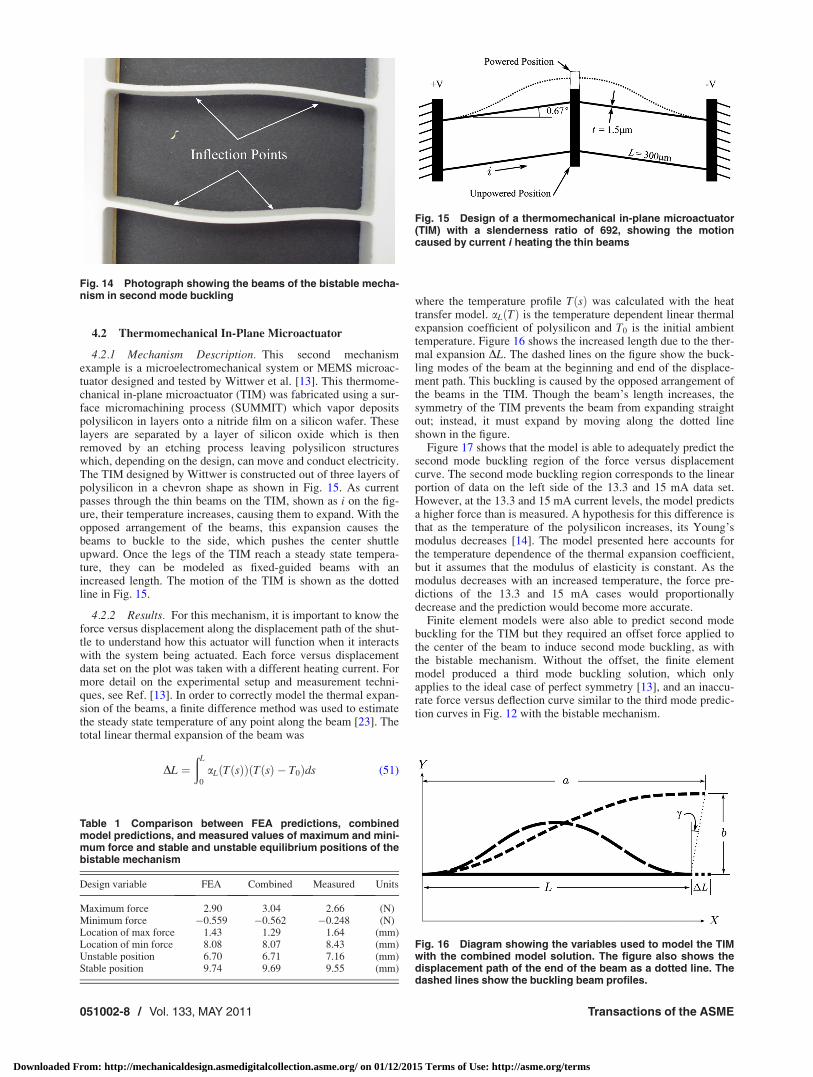
4.2.1 Mechanism Description. This second mechanismexample is a microelectromechanical system or MEMS microac-tuator designed and tested by Wittwer et al. [13]. This thermome-chanical in-plane microactuator (TIM) was fabricated using a sur-face micromachining process (SUMMIT) which vapor depositspolysilicon in layers onto a nitride film on a silicon wafer. Theselayers are separated by a layer of silicon oxide which is thenremoved by an etching process leaving polysilicon structureswhich, depending on the design, can move and conduct electricity.The TIM designed by Wittwer is constructed out of three layers ofpolysilicon in a chevron shape as shown in Fig. 15. As currentpasses through the thin beams on the TIM, shown as i on the fig-ure, their temperature increases, causing them to expand. With theopposed arrangement of the beams, this expansion causes thebeams to buckle to the side, which pushes the center shuttleupward. Once the legs of the TIM reach a steady state tempera-ture, they can be modeled as fixed-guided beams with anincreased length. The motion of the TIM is shown as the dottedline in Fig. 15.

4.2.2 Results. For this mechanism, it is important to know theforce versus displacement along the displacement path of the shut-tle to understand how this actuator will function when it interactswith the system being actuated. Each force versus displacementdata set on the plot was taken with a different heating current. Formore detail on the experimental setup and measurement techni-ques, see Ref. [13]. In order to correctly model the thermal expan-sion of the beams, a finite difference method was used to estimatethe steady state temperature of any point along the beam [23]. Thetotal linear thermal expansion of the beam was

DL ¼ðL

0

aLðTðsÞÞðTðsÞ � T0Þds (51)

where the temperature profile TðsÞ was calculated with the heattransfer model. aLðTÞ is the temperature dependent linear thermalexpansion coefficient of polysilicon and T0 is the initial ambienttemperature. Figure 16 shows the increased length due to the ther-mal expansion DL. The dashed lines on the figure show the buck-ling modes of the beam at the beginning and end of the displace-ment path. This buckling is caused by the opposed arrangement ofthe beams in the TIM. Though the beam’s length increases, thesymmetry of the TIM prevents the beam from expanding straightout; instead, it must expand by moving along the dotted lineshown in the figure.

Figure 17 shows that the model is able to adequately predict thesecond mode buckling region of the force versus displacementcurve. The second mode buckling region corresponds to the linearportion of data on the left side of the 13.3 and 15 mA data set.However, at the 13.3 and 15 mA current levels, the model predictsa higher force than is measured. A hypothesis for this difference isthat as the temperature of the polysilicon increases, its Young’smodulus decreases [14]. The model presented here accounts forthe temperature dependence of the thermal expansion coefficient,but it assumes that the modulus of elasticity is constant. As themodulus decreases with an increased temperature, the force pre-dictions of the 13.3 and 15 mA cases would proportionallydecrease and the prediction would become more accurate.

Finite element models were also able to predict second modebuckling for the TIM but they required an offset force applied tothe center of the beam to induce second mode buckling, as withthe bistable mechanism. Without the offset, the finite elementmodel produced a third mode buckling solution, which onlyapplies to the ideal case of perfect symmetry [13], and an inaccu-rate force versus deflection curve similar to the third mode predic-tion curves in Fig. 12 with the bistable mechanism.

Fig. 14 Photograph showing the beams of the bistable mecha-nism in second mode buckling

Table 1 Comparison between FEA predictions, combinedmodel predictions, and measured values of maximum and mini-mum force and stable and unstable equilibrium positions of thebistable mechanism

Design variable FEA Combined Measured Units

Maximum force 2.90 3.04 2.66 (N)Minimum force �0.559 �0.562 �0.248 (N)Location of max force 1.43 1.29 1.64 (mm)Location of min force 8.08 8.07 8.43 (mm)Unstable position 6.70 6.71 7.16 (mm)Stable position 9.74 9.69 9.55 (mm)

Fig. 15 Design of a thermomechanical in-plane microactuator(TIM) with a slenderness ratio of 692, showing the motioncaused by current i heating the thin beams

Fig. 16 Diagram showing the variables used to model the TIMwith the combined model solution. The figure also shows thedisplacement path of the end of the beam as a dotted line. Thedashed lines show the buckling beam profiles.



5 Conclusions and Recommendations

The model developed here presents a method to predict bucklingbehavior of fixed-guided beams. It combines an elliptic integralmodel for the buckling of a flexible beam with a numerical axialdeflection solution. Together these models provide a method for cal-culating the reaction force of a beam for a given displacement or cal-culating the deflection of a beam given a directional force. In particu-lar, this model is capable of accurately modeling the beam in boththe first and second mode bending regions with a capability of mod-eling the higher modes if desired. The model was used to explore awide deflection space for a fixed-guided beam. The results showeddifferent zones of deflection for first and second mode bending. Thezones are clearly separated using the model. While the model com-pares well with finite element solutions, the finite element modelrequires the application of a spurious offset force to model the secondmode buckling region. These offset forces cause disagreementbetween the two models for regions where the reaction force magni-tude is on the same order of magnitude as the offset force.

Following the development of the model, its predictions were com-pared to two compliant mechanisms whose motion require the beamsto bend in both first and second mode. There is adequate agreementbetween the model and the measured force versus displacement behav-ior of the mechanisms. In both cases the second mode buckling regionshowed a linear force versus deflection relationship that was modeledwell with the analytical model. In addition, non-linear finite elementmodels were shown to produce an incorrect solution unless an unreal-istic transverse load was placed at the center of the beam. To furtherimprove the solution for the bistable mechanism, a correlation toaccount for stress relaxation of the materials could be developed. Also,in the case of the TIM, the temperature dependence of the Young’smodulus could be incorporated. However, despite these minor adjust-ments, the model follows the behavior of real systems and providesinsight into the motion of fixed-guided beams.

Acknowledgment

The assistance of Kevin Cole, Ken Forester, Peter Halverson,and Jonathan Scott in fabrication and testing of the compliantbistable mechanism is gratefully acknowledged.

References[1] Howell, L. L., 2001, Compliant Mechanisms, Wiley, New York.[2] Parkinson, M. B., Jensen, B. D., and Roach, G. M., 2000. “Optimization-Based

Design of a Fully-Compliant Bistable Micromechanism,” ASME Design Engi-neering Technical Conferences and Computers and Information in EngineeringConference, no. DETC2000/MECH-14119.

[3] Ananthasuresh, G. K., and Howell, L. L., 2005, “Mechanical Design of Compli-ant Microsystems—A Perspective and Prospects,” ASME J. Mech. Des., 127,pp. 736–738.

[4] Jensen, B. D., Howell, L. L., and Salmon, L. G., 1999, “Design of Two-Link,In-Plane, Bistable Compliant Micro-Mechanisms,” ASME J. Mech. Des., 121,pp. 416–423.

[5] Jensen, B. D., and Howell, L. L., 2003, “Identification of Compliant Pseudo-Rigid-Body Four-Link Mechanism Configurations Resulting in Bistable Behav-ior,” ASME J. Mech. Des., 125, pp. 701–708.

[6] Qiu, J., Lang, J. H., and Slocum, A. H., 2004, “A Curved-Beam Bistable Mech-anism,” J. Microelectromech. Syst., 13, pp. 137–146.

[7] Awtar, S., Slocum, A. H., and Sevincer, E., 2007, “Charactersitics of Beam-Based Flexure Modules,” ASME J. Mech. Des., 129(6), pp. 625–639.

[8] Awtar, S., and Sen, S., 2010, “A Generalized Constraint Model for Two-Dimen-sional Beam Flexures: Nonlinear Strain Energy Formulation,” ASME J. Mech.Des., 132(8), p. 081009.

[9] Shoup, T. E., and McLarnan, C. W., 1971, “On the Use of the Undulating Elas-tica for the Analysis of Flexible Link Mechanisms,” J. Eng. Ind., 93, pp. 263–267.

[10] Oh, Y. S., and Kota, S., 2008, “Robust Design of Bistable Compliant Mecha-nisms Using the Bistability of a Clamped-Pinned Beam,” ASME 2008 Interna-tional Design Engineering Technical Conferences and Computers andInformation in Engineering Conference, no. DETC2008-49755, pp. 273–282.

[11] Todd, B., Jensen, B. D., Shultz, S. M., and Hawkins, A. R., 2010, “Design andTesting of a Thin-Flexure Bistable Mechanism Suitable for Stamping fromMetal Sheets,” ASME J. Mech. Des., 132, p. 071011.

[12] Tekes�, A., Sonmez, U., and Guvenc, B. A., 2010, “Trajectory Control of Com-pliant Parallel-Arm Mechanisms,” ASME J. Mech. Des., 132, p. 011006.

[13] Wittwer, J. W., Baker, M. S., and Howell, L. L., 2006, “Simulation, Measure-ment, and Asymmetric Buckling of Thermal Microactuators,” Sens. Actuators,A, 128, pp. 395–401.

[14] Shamshirasaz, M., and Asgari, M. B., 2008, “Polysilicon Micro Beams Buck-ling with Temperature-Dependent Properties,” Microsyst. Technol., 14, pp.975–961.

[15] Masters, N. D., and Howell, L. L., 2003, “A Self-Retracting Fully CompliantBistable Micromechanism,” J. Microelectromech. Syst., 12, pp. 273–280.

[16] Messenger, R. K., Aten, Q. T., McLain, T. W., and Howell, L. L., 2010,“Piezoresistive Feedback Control of a MEMS Thermal Actuator,” J. Microelec-tromech. Syst., 18, pp. 1267–1278.

[17] Jensen, B. D., Parkinson, M. B., Kurabayahi, K., Howell, L. L., and Baker, M.S., 2001, “Design Optimization of a Fully-Compliant Bistable Micro-

Fig. 17 Comparison of the force versus displacement data for a thermomechanical in-plane microactuator and the model pre-dictions. The solid lines represent the combined model solution for each heating current.



http://dx.doi.org/10.1115/1.1900150

http://dx.doi.org/10.1115/1.2829477

http://dx.doi.org/10.1115/1.1625399

http://dx.doi.org/10.1109/JMEMS.2004.825308

http://dx.doi.org/10.1115/1.2717231

http://dx.doi.org/10.1115/1.3427884

http://dx.doi.org/10.1115/1.4001876

http://dx.doi.org/10.1115/1.4000637

http://dx.doi.org/10.1016/j.sna.2006.02.014


http://dx.doi.org/10.1109/JMEMS.2003.811751

Mechanism,” ASME International Mechanical Engineering Congress and Expo-sition, no. IMECE001/MEMS-23852.

[18] Zhao, J., Jia, J., He, X., and Wang, H., 2008, “Post-Buckling andSnap-Through Behavior of Inclined Slender Beams,” ASME J. Appl. Mech.,75, p. 041020.

[19] Beyer, W. H., 1979, CRC Standard Mathematical Tables, CRC Press, Inc.[20] Abramowitz, M., and Stegun, I. A., 1972, Handbook of Mathematical Functions

with Formulas, Graphs, and Mathematical Tables, U.S. Government PrintingOffice.

[21] Pendleton, T. M., 2006, “Design and Fabrication of Rotationally Tristable Com-pliant Mechanisms,” Master’s thesis, Brigham Young University.

[22] Dutta, N. K., and Edward, G. H., 1997, “Generic Relaxation Spectra of SolidPolymers. I Development of Spectral Distribution Model and its Applicationto Stress Relaxation of Polypropylene,” J. Appl. Polym. Sci., 66, pp. 1101–1115.

[23] Teichert, K., and Jensen, B., 2008, “Thermal Correction Values forAnalysis of Lineshape Microstructure Arrays,” Sens. Actuators, A, 148, pp.168–175.



http://dx.doi.org/10.1002/(SICI)1097-4628(19971107)66:6<>1.0.CO;2-1


Modeling and Experiments of Buckling Modes and Deflection ...

Documents

Transcript of Modeling and Experiments of Buckling Modes and Deflection ...