Modeling and Control of an Unmanned Underwater · PDF fileModeling and Control of an Unmanned...

i

University of Canterbury University of Technology Eindhoven

Department of Mechanical Engineering Department of Mechanical Engineering

Christchurch, New Zealand Eindhoven, The Netherlands

Modeling and Control of an

Unmanned Underwater Vehicle

J.H.A.M. Vervoort

DCT.2009.096

ii

Master traineeship report

Title: Modeling and Control of an Unmanned Underwater Vehicle

Student: J.H.A.M. Vervoort ID number: 0577316 [TU/e]

236146 [UC]

Supervisor: Prof. Dr. H. Nijmeijer [TU/e]

Coach: Dr. W. Wang [UC]

Host University: University of Canterbury [UC]

Department of Mechanical Engineering, Mechatronics

Sending University: University of technology Eindhoven [TU/e]

Department of Mechanical Engineering, Dynamics and Control

Group

Christchurch, New Zealand, November 2008

iv

Abstract

The Unmanned Underwater Vehicle (UUV) designed at the Mechanical

Engineering Department of the University of Canterbury is in an early stage of

development. With the design of the AUV completed, the primary focus now is to design

control software. The control software has to be able to stabilize the vehicle at a desired

position and let the vehicle follow a desired trajectory within a reasonable error.

The AUV is able to operate in six degrees of freedom and the dynamics of an

AUV are nonlinear and subjected to a variety of disturbances. A kinematic and dynamic

model of the AUV is derived for the six degrees of freedom operating range. The degrees

of freedom are decoupled, where only the surge, heave and yaw degrees of freedom will

be controlled. A system identification approach is proposed to estimate unknown

mass/inertia and damping parameters, treating the surge, heave and yaw degrees of

freedom separately. Unfortunately due to sensor malfunctioning the unknown

mass/inertia and damping terms could not be estimated, a parameter selection method is

used instead. The parameter selection is based on parameter estimation results of software

programs and a parameter comparison with other similar shaped AUVs.

A feedback linearizing control technique is chosen to design control laws for

control in the surge, heave and yaw degrees of freedom. The controller performed well

under parameter perturbation and noise contamination on the feedback position and

velocity signals. An under-actuated control problem arises in x-y plane, since one is only

able to control two degrees of freedom while the AUV has three degrees of freedom. To

steer the AUV smoothly, a path planning model is derived, which describes a path from

A to B with the use of polar coordinates. It works as expected, except for planning a

straight line trajectory due to singularity reasons.

v

The under-actuated control problem is again investigated, assuming sway motion of the

AUV is not negligible, so Coriolis and centripetal forces need to be considered. A state

feedback control method is explained, which is able to follow a reference trajectory in the

x-y plane. The only disadvantage is that the yaw degree of freedom of the reference

trajectory needs to be persistently exciting, which makes following a straight line

impossible.

vi

Contents

1 Introduction 1

2 Kinematic and Dynamic Model of the AUV 5

2.1 AUV Kinematics 5

2.1.1 Reference Frames 5

2.1.2 Euler Angles 7

2.1.3 State Space Representation of the AUV 7

2.1.4 State Vector Transformation 7

2.1.4.1 Position State Vector Transformation 8

2.1.4.1 Velocity State Vector Transformation 9

2.2 Dynamic Model of the AUV 10

2.2.1 Mass and Inertia Matrix 11

2.2.2 Coriolis and Centripetal Matrix 13

2.2.3 Hydrodynamic Damping Matrix 14

2.2.4 Gravitational and Buoyancy Matrix 15

2.2.5 Force and Torque Vector 15

3 System Identification of the AUV 17

3.1 Assumptions on the AUV Dynamics 17

3.2 Parameter Estimation, a System Identification Approach 19

3.3 Parameter Selection 21

vii

4 Control of AUVs 25

4.1 Control Problems 25

4.2 Feedback Linearization 26

4.2.1 Derivation of the Feedback Linearization 26

4.2.2 Tracking 29

4.2.3 Simulation Results 30

4.3 Path Planning 33

4.3.1 A Path Planning Method 34

4.3.3 Simulation Results 38

4.4 Summary 40

5 Tracking Control of an Under-Actuated AUV 45

5.1 An Under-Actuated AUV 45

5.2 Simulation Results 50

5.3 Summary 53

6 Conclusions & Recommendations 55

6.1 Conclusions 55

6.2 Recommendations 57

Bibliography 59

Appendices 65

A Appendix A 65

B Appendix B 67

C Appendix C 77

D Appendix D 79

E Appendix E 83

F Appendix F 87

G Appendix G 91

H Appendix H 95

I Appendix I 99

J Appendix J 105

K Appendix K 107

1

Chapter 1

Introduction

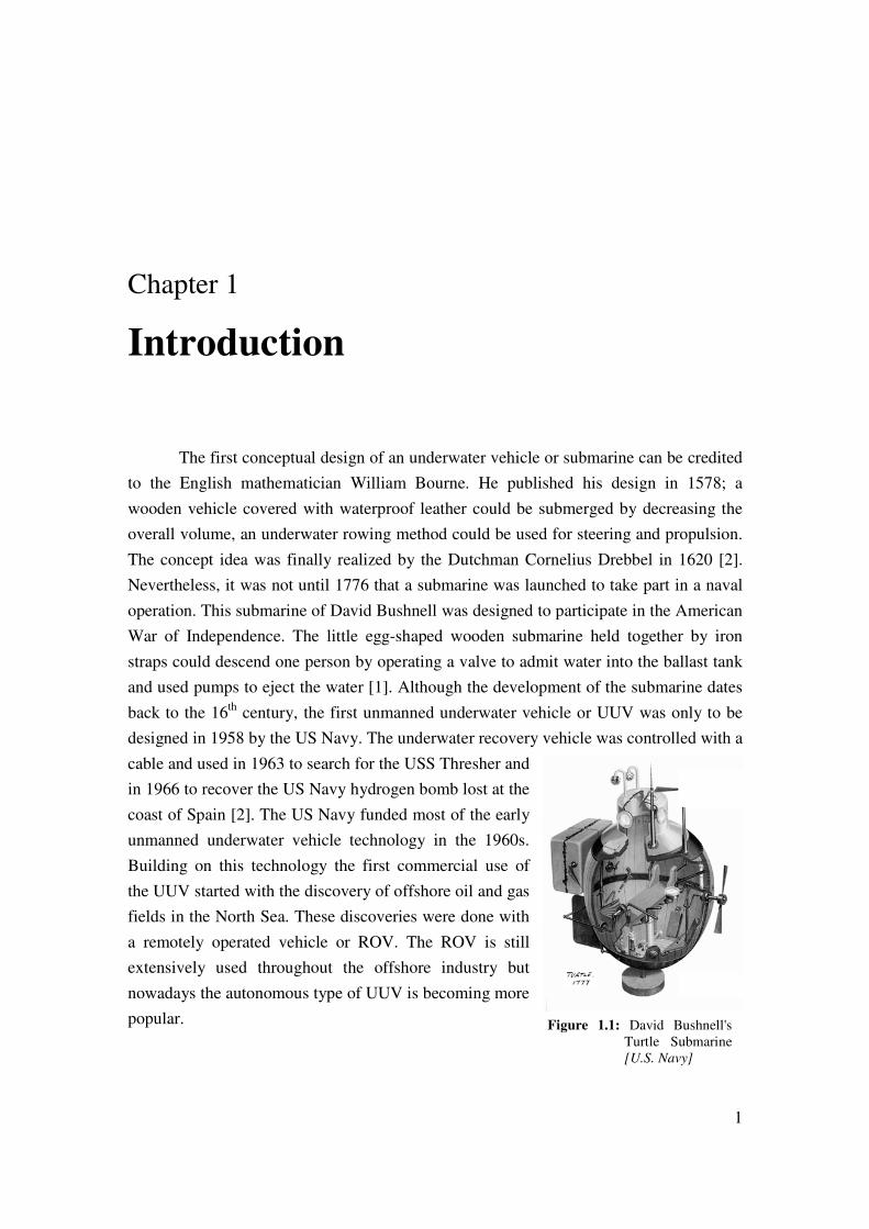
The first conceptual design of an underwater vehicle or submarine can be credited

to the English mathematician William Bourne. He published his design in 1578; a

wooden vehicle covered with waterproof leather could be submerged by decreasing the

overall volume, an underwater rowing method could be used for steering and propulsion.

The concept idea was finally realized by the Dutchman Cornelius Drebbel in 1620 [2].

Nevertheless, it was not until 1776 that a submarine was launched to take part in a naval

operation. This submarine of David Bushnell was designed to participate in the American

War of Independence. The little egg-shaped wooden submarine held together by iron

straps could descend one person by operating a valve to admit water into the ballast tank

and used pumps to eject the water [1]. Although the development of the submarine dates

back to the 16th

century, the first unmanned underwater vehicle or UUV was only to be

designed in 1958 by the US Navy. The underwater recovery vehicle was controlled with a

cable and used in 1963 to search for the USS Thresher and

in 1966 to recover the US Navy hydrogen bomb lost at the

coast of Spain [2]. The US Navy funded most of the early

unmanned underwater vehicle technology in the 1960s.

Building on this technology the first commercial use of

the UUV started with the discovery of offshore oil and gas

fields in the North Sea. These discoveries were done with

a remotely operated vehicle or ROV. The ROV is still

extensively used throughout the offshore industry but

nowadays the autonomous type of UUV is becoming more

popular. Figure 1.1: David Bushnell's

Turtle Submarine

[U.S. Navy]

2

The term UUV is a generic expression to describe both remotely operated and

autonomous underwater vehicles. The difference between an autonomous underwater

vehicle, or AUV, and a ROV is that the ROV is connected to a command platform (for

instance a ship) with a tethered cable or an acoustic link [3]. The tethered cable ensures

energy supply and information signals, in this way an operator is able to constantly

monitor and control the vehicle. The AUV however, is equipped with a battery pack and

sonar to fulfill its mission avoiding the use of an operator, which introduces conflicting

control requirements. It has to be simple enough to ensure an online implementation of

control techniques but at the same time has to cope with a time-varying

vehicle/environment interaction [4].

Nowadays the AUV is becoming more and more popular since it can operate and

explore in extreme depths (which is useful for the offshore industry) while at the same

time it is a low-cost alternative capable of undertaking surveillance missions or mine

laying and disposal operations for the navy [2].

The term AUV covers two different groups of vehicles, namely flight vehicles and

hovering vehicles. Flight vehicles are often used for surveys, searches, object delivery

and object location, while hovering vehicles are used for detailed inspection and physical

work around fixed objects [6][7].

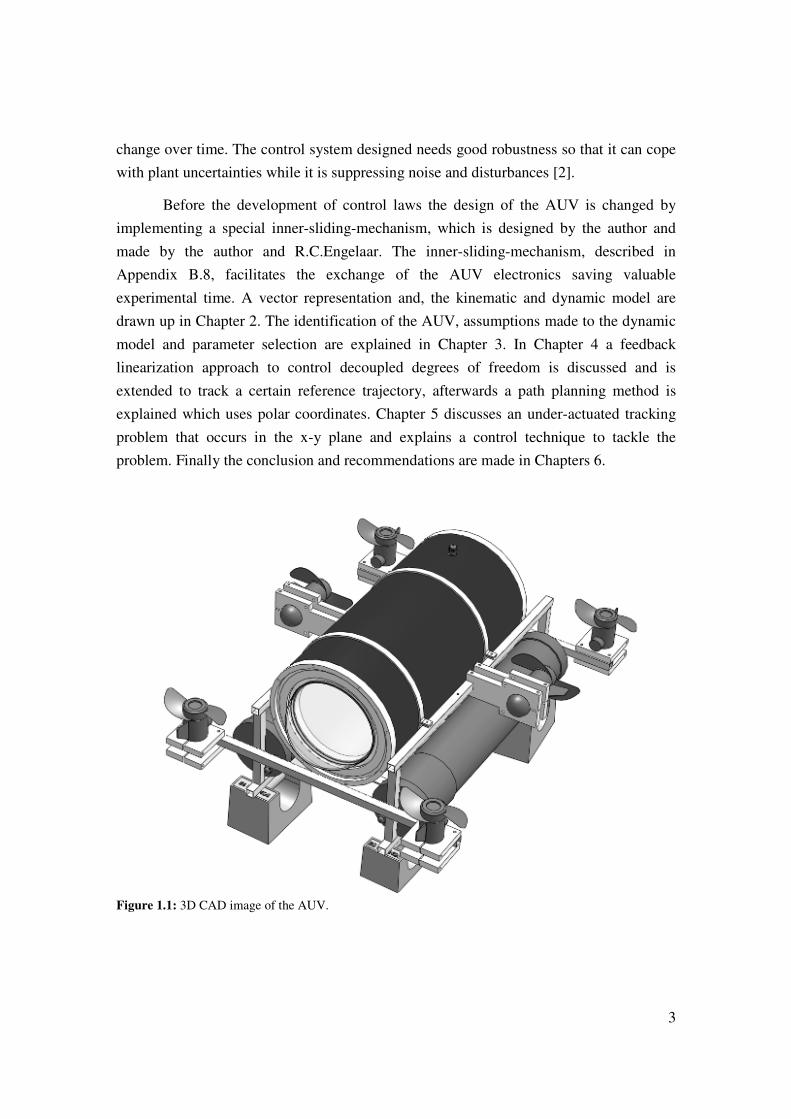
The AUV designed at the Mechanical Engineering Department of the University

of Canterbury is a hovering AUV, see Figure 1.1. The basic design consists of a

cylindrical PVC hull with aluminum end caps, a buoyancy system based on a dynamic

diving method, four vertical and two horizon thrusters, a pressure sensor, an inertia

measurement unit (IMU), motor controllers, batteries and a motherboard. More

information about the design of the AUV can be found in Appendix B. The AUV has to

be capable of self navigation, object detection, object avoidance and artificial intelligence

to carry out simple tasks [5]. The final goal is to use the AUV for ship hull inspection in

harbors. However the development of the AUV is in an early stage. With the design of

the AUV completed, the primary focus now is to design control software. The control

software has to be able to stabilize the vehicle at a desired position and let the vehicle

follow a desired trajectory within a reasonable error. The AUV is able to operate in six

degrees of freedom and the dynamics of an AUV are nonlinear and subjected to a variety

of disturbances. The development of suitable algorithms for motion and position control

of an AUV is a challenging task. When in operation the characteristics of the AUV will

3

change over time. The control system designed needs good robustness so that it can cope

with plant uncertainties while it is suppressing noise and disturbances [2].

Before the development of control laws the design of the AUV is changed by

implementing a special inner-sliding-mechanism, which is designed by the author and

made by the author and R.C.Engelaar. The inner-sliding-mechanism, described in

Appendix B.8, facilitates the exchange of the AUV electronics saving valuable

experimental time. A vector representation and, the kinematic and dynamic model are

drawn up in Chapter 2. The identification of the AUV, assumptions made to the dynamic

model and parameter selection are explained in Chapter 3. In Chapter 4 a feedback

linearization approach to control decoupled degrees of freedom is discussed and is

extended to track a certain reference trajectory, afterwards a path planning method is

explained which uses polar coordinates. Chapter 5 discusses an under-actuated tracking

problem that occurs in the x-y plane and explains a control technique to tackle the

problem. Finally the conclusion and recommendations are made in Chapters 6.

Figure 1.1: 3D CAD image of the AUV.

5

Chapter 2

Kinematic and Dynamic Model of the AUV

The existence of several complex and nonlinear forces acting upon an underwater

vehicle, especially with open frame AUVs, makes the control of AUVs trickier. Several

complex and nonlinear forces are, for example, hydrodynamic drag, damping, lift forces,

Coriolis and centripetal forces, gravity and buoyancy forces, thruster forces, and

environmental disturbances [17]. The kinematics and dynamics which are involved in

controlling and modeling an AUV are explored in this chapter. The first section about the

kinematics of the AUV will explain the reference frames, Euler angles and the state space

representation. The second section about the dynamics will explain the dynamic model of

the AUV, with a description of the mass and inertia, Coriolis and centripetal,

hydrodynamic damping, and, gravitation and buoyancy forces.

2.1 AUV Kinematics

The reference frames, the use of Euler angles and the state space representation of

the AUV will be explained in the following subsections.

2.1.1 Reference Frames

Two reference frames are introduced to model the AUV, a world-fixed reference

frame (W) and a body-fixed reference frame (B). The W-frame is coupled to the world,

where the x-axis points to the north, the y-axis to the east and the z-axis to the center of

the earth. The B-frame is coupled to the vehicle, where the x-axis points to the forward

direction, the y-axis to the right of the vehicle and the z-axis vertically down. The W-

6

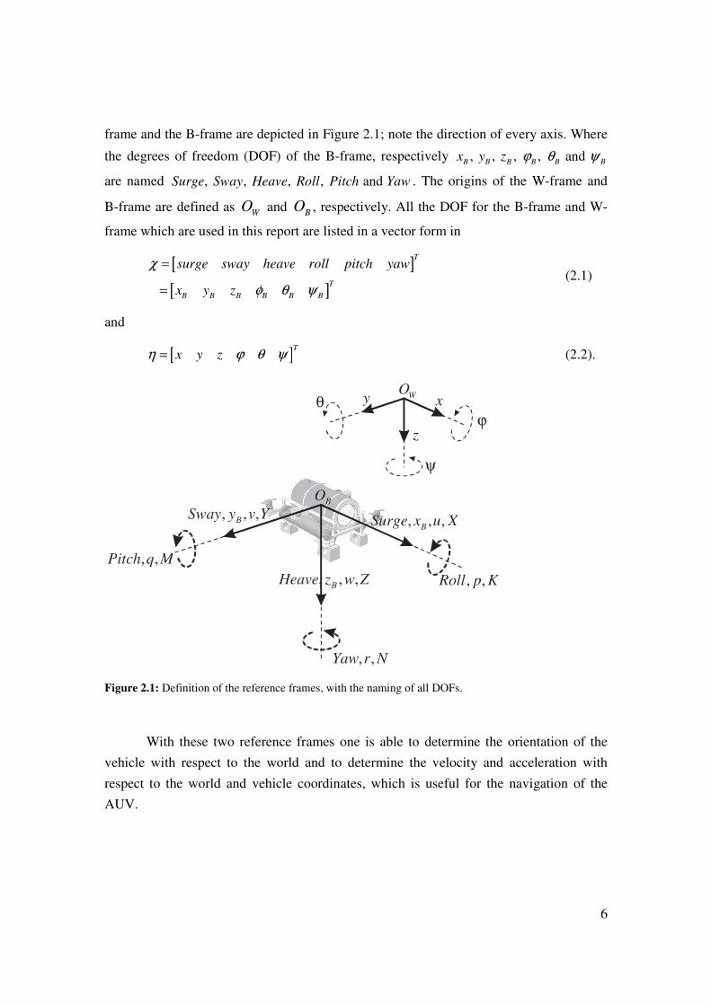
frame and the B-frame are depicted in Figure 2.1; note the direction of every axis. Where

the degrees of freedom (DOF) of the B-frame, respectively , , , , and B B B B B Bx y z ϕ θ ψ

are named , , , , and Surge Sway Heave Roll Pitch Yaw . The origins of the W-frame and

B-frame are defined as W

O and B

O , respectively. All the DOF for the B-frame and W-

frame which are used in this report are listed in a vector form in

[ ]

[ ]

T

T

B B B B B B

surge sway heave roll pitch yaw

x y z

χ

φ θ ψ

=

= (2.1)

and

[ ] T

x y zη ϕ θ ψ= (2.2).

ϕθ

ψ

xy

z

, ,Pitch q M

, , ,BSway y v Y

, ,Roll p K

, , ,BSurge x u X

, ,Yaw r N

, , ,BHeave z w Z

BO

WO

Figure 2.1: Definition of the reference frames, with the naming of all DOFs.

With these two reference frames one is able to determine the orientation of the

vehicle with respect to the world and to determine the velocity and acceleration with

respect to the world and vehicle coordinates, which is useful for the navigation of the

AUV.

7

2.1.2 Euler Angles

Euler angles relate two coordinate systems in terms of orientation, i.e. the

orientation of the B-frame with respect to the W-frame. To orientate one coordinate

system with respect to another it may be subjected to a sequence of three rotations, the

Euler convention used to describe the orientation from body to world is the z-y-x

convention. The B-frame is first rotated around the z-axis, then around the y-axis and then

around the x-axis, this corresponds to the rotation angles of yaw (ψ ), pitch (θ ), and roll

(φ ), respectively. The rotation matrix used to describe the orientation of the B-frame with

respect to the W-frame is given by

30 32 21 10( , , ) ( ) ( ) ( ) or ( , , ) ( ) ( ) ( )BW

z y xR R R R R R R Rϕ θ ψ ψ θ ϕ ϕ θ ψ ψ θ ϕ= = (3.3).

The complete derivation of the rotation matrix can be found in Appendix A.1.

2.1.3 State Space Representation of the AUV

A state space representation is defined to provide a compact way to model and

analyze the AUV. The vector notation includes the position vectors χ (2.1) and η (2.2)

for the B and W-frame; the velocity vectors ν and η& for the B and W-frame, respectively

[ ]T T

B B B B B Bx y z u v w p q rν φ θ ψ = = & & && & & (2.4.a)

and

T

x y zη φ θ ψ = & && && & & (2.4.b);

and the force/torque vector τ of the thruster input,

T

u v w ϕ θ ψτ τ τ τ τ τ τ = (2.4.c).

2.1.4 State Vector Transformation

The transformation of the position, velocity and acceleration vector from the B-

frame to the W-frame is presented in the following subsections.

8

0

1er

0

2er

0

3er

1

3er

1

1er

1

2er

2

1er

2

2er

2

3er

3

1er

3

2er

3

3er

θ

4

3er

4

2er

4

1er

trW BO O=

B

A

W BO O=

ψϕ

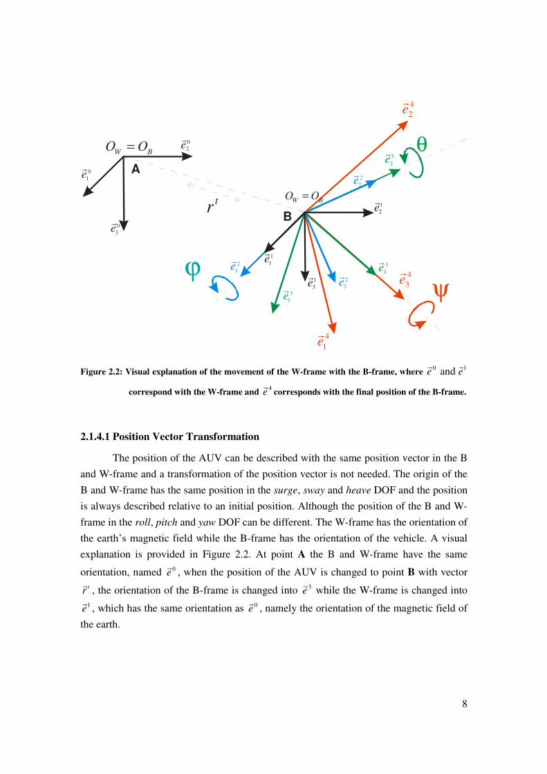
Figure 2.2: Visual explanation of the movement of the W-frame with the B-frame, where 0 1 and e e

r r

correspond with the W-frame and 4

er

corresponds with the final position of the B-frame.

2.1.4.1 Position Vector Transformation

The position of the AUV can be described with the same position vector in the B

and W-frame and a transformation of the position vector is not needed. The origin of the

B and W-frame has the same position in the surge, sway and heave DOF and the position

is always described relative to an initial position. Although the position of the B and W-

frame in the roll, pitch and yaw DOF can be different. The W-frame has the orientation of

the earth’s magnetic field while the B-frame has the orientation of the vehicle. A visual

explanation is provided in Figure 2.2. At point A the B and W-frame have the same

orientation, named 0er

, when the position of the AUV is changed to point B with vector

trr

, the orientation of the B-frame is changed into 3er

while the W-frame is changed into

1er

, which has the same orientation as 0er

, namely the orientation of the magnetic field of

the earth.

9

2.1.4.1 Velocity Vector Transformation

The velocity vector consists of linear and angular velocities, the velocity vector

can be transformed from the B-frame into the W-frame with the use of

( )Jη η ν=& with [ ]T

W Wη υ ω=& , (2.5)

[ ]T

B Bν υ ω= ,

1

2

( ) 0( )

0 ( )

W

W

JJ

J

υη

ω

=

.

where, ν is the velocity vector of the B-frame, η& is the velocity vector of the W-frame,

Bυ is the linear velocity of the B-frame, Bω is the angular velocity vector of the B-frame,

Wυ is the linear velocity of the W-frame, Wω is the angular velocity of the W-frame,

( )J η is the coordinate transform matrix, which brings the W-frame into alignment with

the B-frame.

The world linear velocities or accelerations can be calculated from the body linear

velocities with the use of

1 1 ( ) with ( ) ( )BW

W W B W WJ J Rν ν ν ν ν= = (2.6)

where

1

( ) ( ) ( ) ( ) ( ) ( ) ( ) ( ) ( ) ( ) ( ) ( )

( ) ( ) ( ) ( ) ( ) ( ) ( ) ( ) ( ) ( ) ( ) ( ) ( )

( ) ( ) ( ) ( ) ( )

W

C C C S S S C S S C S C

J C S C C S S S S C C S S

S S C C C

θ ψ ϕ ψ ϕ θ ψ ϕ ψ ϕ θ ψ

ν θ ψ ϕ ψ ϕ θ ψ ϕ ψ ϕ θ ψ

θ ϕ θ ϕ θ

− + + = + − + −

note that the rotation matrix (2.3) is being used.

The world angular velocities or accelerations can be calculated from the body

angular velocities with the use of

2 2

1 ( ) ( ) ( ) ( )

( ) with ( ) 0 ( ) ( )

0 ( ) / ( ) ( ) / ( )

W W B W

S T C T

J J C S

S C C C

ϕ θ ϕ θ

ω ω ω ω ϕ ϕ

ϕ θ ϕ θ

= = −

r r (2.7)

10

where S denotes sine, C denotes cosine and T denotes tangent. The full derivation of 2J

can be found in Appendix A.2. Note that 2J is undefined if2

πθ = ± , which results in a

singularity of the system kinematic equation and that 1

2 2

TJ J− ≠ . The coordinate

transformation matrix J is still defined in Euler angles, since the AUV is unlikely to ever

pitch anywhere near 2

π± ( 90± o ). If in future applications the AUV needs to operate near

to this singularity two Euler angle representations with different singularities can be used

to avoid the singular point by simply switching between these. Another possibility is to

use a quaternion representation [37, 38].

2.2 Dynamic Model of the AUV

The dynamic model for the AUV is defined to be able to formulate control

algorithms and to perform simulations. The dynamic model

( ) ( ) ( )M C D gν ν ν ν ν η τ+ + + =& (2.8)

is derived from the Newton-Euler equation of a rigid body in fluid [8, 9]. Where

RB AM M M= + is the inertia matrix for the rigid body and added mass, respectively;

( ) ( ) ( )RB AC C Cν ν ν= + is the Coriolis and centripetal matrix for the rigid body and added

mass, respectively; ( ) ( ) ( )q lD D Dν ν ν= + is the quadratic and linear drag matrix,

respectively; ( )g η is the gravitational and buoyancy matrix; τ is the force/torque vector

of the thruster input. Note that (2.8) does not take into account environmental

disturbances, such as underwater currents. The dynamic model which includes the

environmental disturbances is given in Appendix C.

The hydrodynamic forces and moments where an AUV is dealing with can be

separated into added mass and hydrodynamic damping. Added mass is a pressure-

induced force and/or moment, which is generated by the forced motion of the vehicle

body. Added mass can also be understood as a finite amount of water connected to the

vehicle such that the mass of the AUV appears larger [16]. The forces generated by

hydrodynamic damping, mass and inertia, Coriolis and centripetal, and, gravitation and

buoyancy are explained in the following subsections.

11

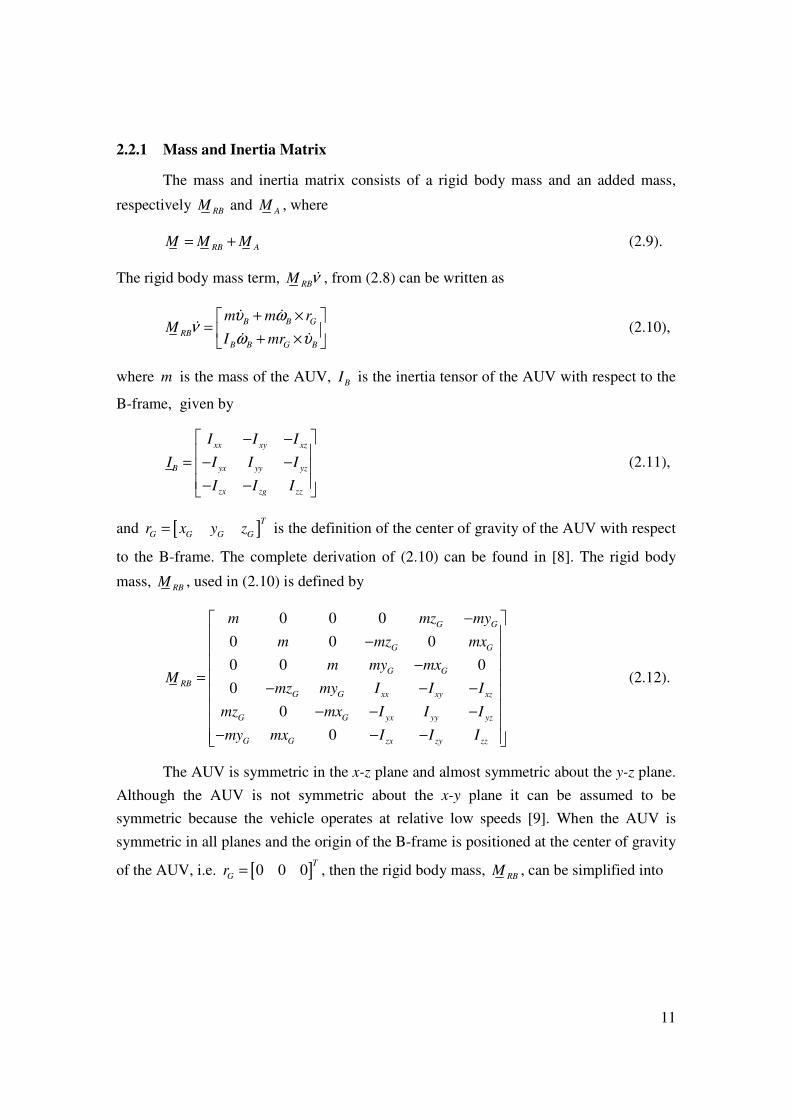
2.2.1 Mass and Inertia Matrix

The mass and inertia matrix consists of a rigid body mass and an added mass,

respectively RBM and AM , where

RB AM M M= + (2.9).

The rigid body mass term, RBM ν& , from (2.8) can be written as

B B G

RB

B B G B

m m rM

I mr

υ ων

ω υ

+ × = + ×

& &&

& & (2.10),

where m is the mass of the AUV, BI is the inertia tensor of the AUV with respect to the

B-frame, given by

xx xy xz

B yx yy yz

zx zg zz

I I I

I I I I

I I I

− −

= − − − −

(2.11),

and [ ]T

G G G Gr x y z= is the definition of the center of gravity of the AUV with respect

to the B-frame. The complete derivation of (2.10) can be found in [8]. The rigid body

mass, RBM , used in (2.10) is defined by

0 0 0

0 0 0

0 0 0

0

0

0

G G

G G

G G

RB

G G xx xy xz

G G yx yy yz

G G zx zy zz

m mz my

m mz mx

m my mxM

mz my I I I

mz mx I I I

my mx I I I

− − −

= − − −

− − − − − −

(2.12).

The AUV is symmetric in the x-z plane and almost symmetric about the y-z plane.

Although the AUV is not symmetric about the x-y plane it can be assumed to be

symmetric because the vehicle operates at relative low speeds [9]. When the AUV is

symmetric in all planes and the origin of the B-frame is positioned at the center of gravity

of the AUV, i.e. [ ]0 0 0T

Gr = , then the rigid body mass, RBM , can be simplified into

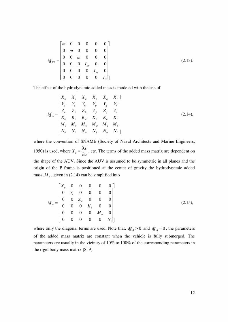
12

0 0 0 0 0

0 0 0 0 0

0 0 0 0 0

0 0 0 0 0

0 0 0 0 0

0 0 0 0 0

RB

xx

yy

zz

m

m

mM

I

I

I

=

(2.13).

The effect of the hydrodynamic added mass is modeled with the use of

u v w p q r

u v w p q r

u v w p q r

A

u v w p q r

u v w p q r

u v w p q r

X X X X X X

Y Y Y Y Y Y

Z Z Z Z Z ZM

K K K K K K

M M M M M M

N N N N N N

=

& & & & & &

& & & & & &

& & & & & &

& & & & & &

& & & & & &

& & & & & &

(2.14),

where the convention of SNAME (Society of Naval Architects and Marine Engineers,

1950) is used, whereu

XX

u

∂=

∂&

&, etc. The terms of the added mass matrix are dependent on

the shape of the AUV. Since the AUV is assumed to be symmetric in all planes and the

origin of the B-frame is positioned at the center of gravity the hydrodynamic added

mass, AM , given in (2.14) can be simplified into

0 0 0 0 0

0 0 0 0 0

0 0 0 0 0

0 0 0 0 0

0 0 0 0 0

0 0 0 0 0

u

v

w

A

p

q

r

X

Y

ZM

K

M

N

=

&

&

&

&

&

&

(2.15),

where only the diagonal terms are used. Note that, 0AM > and 0A

M =& , the parameters

of the added mass matrix are constant when the vehicle is fully submerged. The

parameters are usually in the vicinity of 10% to 100% of the corresponding parameters in

the rigid body mass matrix [8, 9].

13

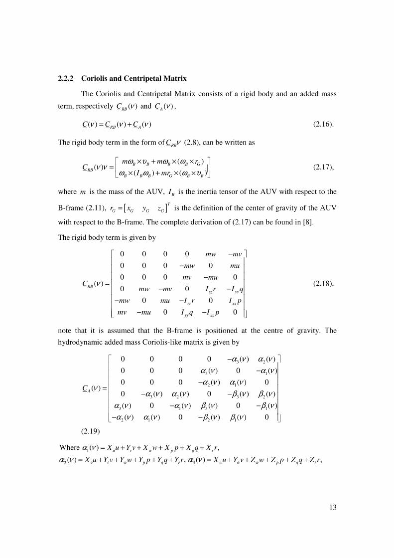
2.2.2 Coriolis and Centripetal Matrix

The Coriolis and Centripetal Matrix consists of a rigid body and an added mass

term, respectively ( )RBC ν and ( )AC ν ,

( ) ( ) ( )RB AC C Cν ν ν= + (2.16).

The rigid body term in the form of RBC ν (2.8), can be written as

( )( )

( ) ( )

B B B B G

RB

B B B G B B

m m rC

I mr

ω υ ω ων ν

ω ω ω υ

× + × × = × + × ×

(2.17),

where m is the mass of the AUV, BI is the inertia tensor of the AUV with respect to the

B-frame (2.11), [ ]T

G G G Gr x y z= is the definition of the center of gravity of the AUV

with respect to the B-frame. The complete derivation of (2.17) can be found in [8].

The rigid body term is given by

0 0 0 0

0 0 0 0

0 0 0 0( )

0 0

0 0

0 0

RB

zz yy

zz xx

yy xx

mw mv

mw mu

mv muC

mw mv I r I q

mw mu I r I p

mv mu I q I p

ν

− − −

= − −

− −

− −

(2.18),

note that it is assumed that the B-frame is positioned at the centre of gravity. The

hydrodynamic added mass Coriolis-like matrix is given by

3 2

3 1

2 1

3 2 3 2

3 1 3 1

2 1 2 1

0 0 0 0 ( ) ( )

0 0 0 ( ) 0 ( )

0 0 0 ( ) ( ) 0( )

0 ( ) ( ) 0 ( ) ( )

( ) 0 ( ) ( ) 0 ( )

( ) ( ) 0 ( ) ( ) 0

AC

α ν α ν

α ν α ν

α ν α νν

α ν α ν β ν β ν



− − −

= − −

− − − −

(2.19)

1Where ( ) ,u v w p q r

X u Y v X w X p X q X rα ν = + + + + +& & & & & &

2 ( ) ,v v w p q rX u Y v Y w Y p Y q Y rα ν = + + + + +& & & & & & 3( ) ,w w w p q rX u Y v Z w Z p Z q Z rα ν = + + + + +& & & & & &

14

1( ) ,p p p p q r

X u Y v Z w K p K q K rβ ν = + + + + +& & & & & & 2 ( )q q q q q r

X u Y v Z w K p M q M rβ ν = + + + + +& & & & & &

and 3( ) ,r r r r r rX u Y v Z w K p M q N rβ ν = + + + + +& & & & & & also here the SNAME notation is used.

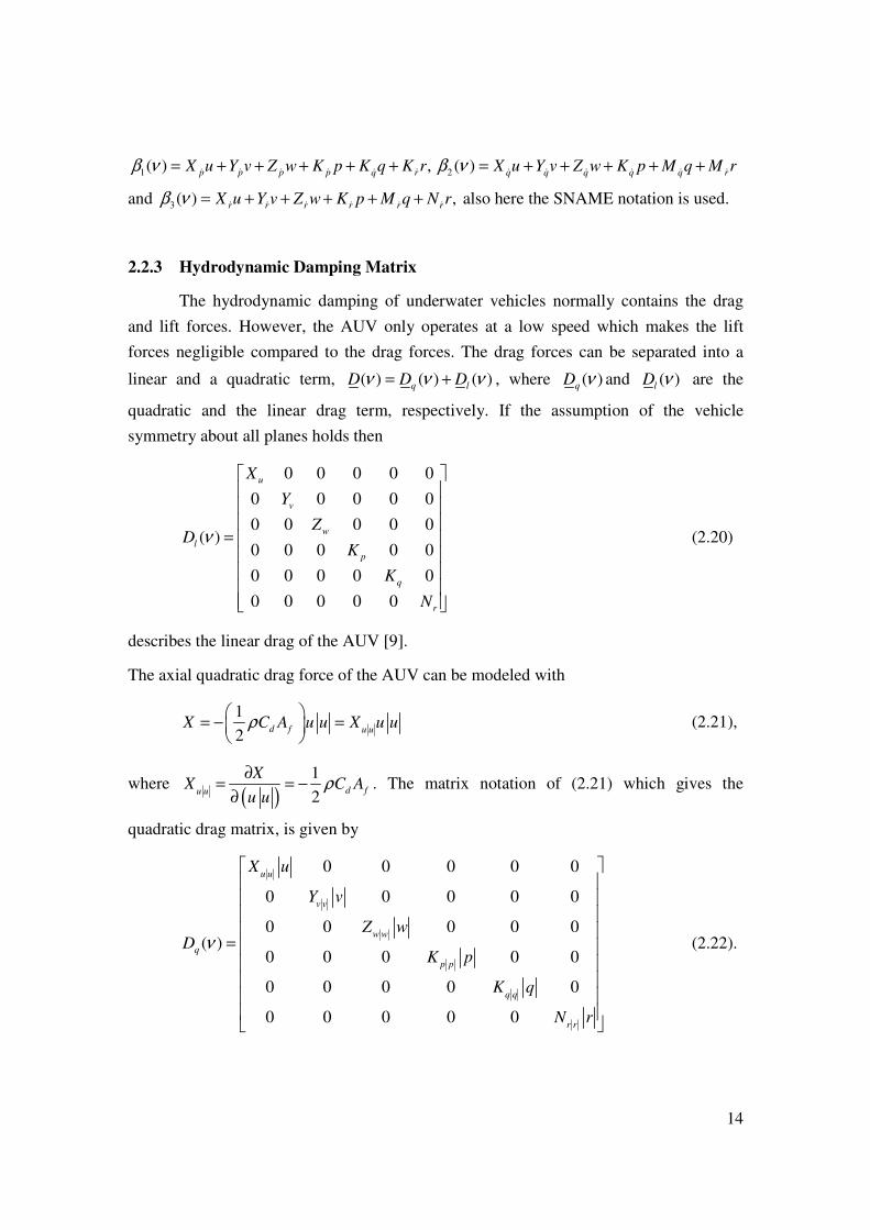
2.2.3 Hydrodynamic Damping Matrix

The hydrodynamic damping of underwater vehicles normally contains the drag

and lift forces. However, the AUV only operates at a low speed which makes the lift

forces negligible compared to the drag forces. The drag forces can be separated into a

linear and a quadratic term, ( ) ( ) ( )q lD D Dν ν ν= + , where ( )qD ν and ( )lD ν are the

quadratic and the linear drag term, respectively. If the assumption of the vehicle

symmetry about all planes holds then

0 0 0 0 0

0 0 0 0 0

0 0 0 0 0( )

0 0 0 0 0

0 0 0 0 0

0 0 0 0 0

u

v

w

l

p

q

r

X

Y

ZD

K

K

N

ν

=

(2.20)

describes the linear drag of the AUV [9].

The axial quadratic drag force of the AUV can be modeled with

1

2d f u u

X C A u u X u uρ

= − =

(2.21),

where ( )

1

2d fu u

XX C A

u uρ

∂= = −

∂. The matrix notation of (2.21) which gives the

quadratic drag matrix, is given by

0 0 0 0 0

0 0 0 0 0

0 0 0 0 0( )

0 0 0 0 0

0 0 0 0 0

0 0 0 0 0

u u

v v

w w

q

p p

q q

r r

X u

Y v

Z wD

K p

K q

N r

ν

=

(2.22).

15

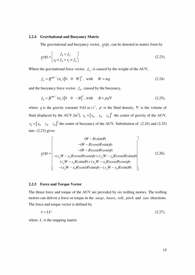
2.2.4 Gravitational and Buoyancy Matrix

The gravitational and buoyancy vector, ( )g η , can be denoted in matrix form by

( )B G

B B G G

f fg

r f r fη

+ = × + ×

(2.23),

Where the gravitational force vector, Gf , is caused by the weight of the AUV,

[ ]1

( ) 0 0TBW

G wf R Wυ−

= , with W mg= (2.24)

and the buoyancy force vector, Bf , caused by the buoyancy,

[ ]1

( ) 0 0TBW

B wf R Bυ−

= − , with B gρ= ∇ (2.25),

where g is the gravity constant 29.81 /m s , ρ is the fluid density, ∇ is the volume of

fluid displaced by the AUV [m3], [ ]

T

G B B Br x y z= the center of gravity of the AUV,

[ ]T

B B B Br x y z= the center of buoyancy of the AUV. Substitution of (2.24) and (2.25)

into (2.23) gives

( )sin( )

( ) cos( )sin( )

( ) cos( ) cos( )( )

( ) cos( )cos( ) ( ) cos( )sin( )

( ) sin( ) ( ) cos( )cos( )

( ) cos( )sin( ) ( ) sin( )

g b g b

g b g b

g b g b

W B

W B

W Bg

y W y B z W z B

z W z B x W x B

x W x B y W y B

θ

θ φ

θ φη

θ φ θ φ

θ θ φ

θ φ θ

− − − − −

= − − + − − + −

− − − −

(2.26).

2.2.5 Force and Torque Vector

The thrust force and torque of the AUV are provided by six trolling motors. The trolling

motors can deliver a force or torque in the , , , surge heave roll pitch and yaw directions.

The force and torque vector is defined by

LUτ = (2.27),

where L is the mapping matrix

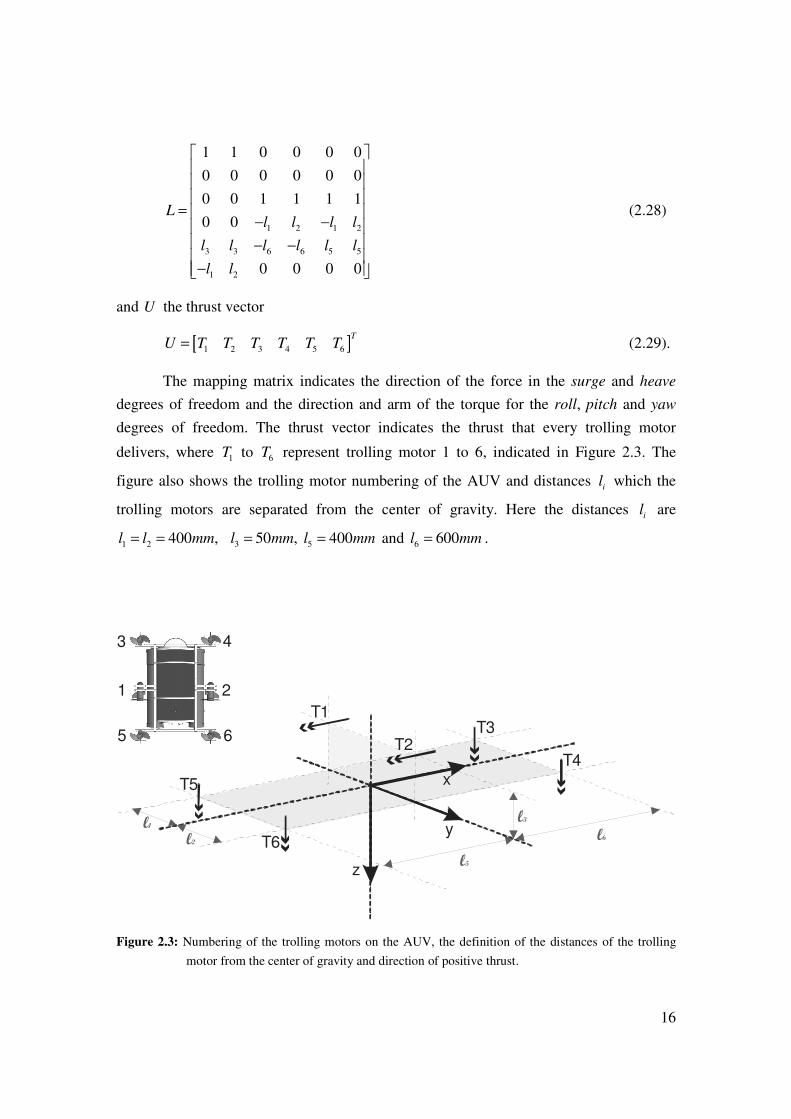
16

1 2 1 2

3 3 6 6 5 5

1 2

1 1 0 0 0 0

0 0 0 0 0 0

0 0 1 1 1 1

0 0

0 0 0 0

Ll l l l

l l l l l l

l l

= − −

− − −

(2.28)

and U the thrust vector

[ ]1 2 3 4 5 6

TU T T T T T T= (2.29).

The mapping matrix indicates the direction of the force in the surge and heave

degrees of freedom and the direction and arm of the torque for the roll, pitch and yaw

degrees of freedom. The thrust vector indicates the thrust that every trolling motor

delivers, where 1T to 6T represent trolling motor 1 to 6, indicated in Figure 2.3. The

figure also shows the trolling motor numbering of the AUV and distances il which the

trolling motors are separated from the center of gravity. Here the distances il are

1 2 400 ,l l mm= = 3 5 50 , 400l mm l mm= = and 6 600l mm= .

x

y

z

T1

T2T3

T4

T5

T6

l1

l2

l3

l5

l6

Figure 2.3: Numbering of the trolling motors on the AUV, the definition of the distances of the trolling

motor from the center of gravity and direction of positive thrust.

1 2

3 4

5 6

17

Chapter 3

System Identification of the AUV

The dynamic model of the AUV introduced in Chapter 2 is a complex model, which is

simplified with a number of assumptions. This chapter will first sum the assumptions

made for the dynamic model and explain why these assumptions can be made.

Afterwards the chapter explains the parameter estimation, where the main problem is

overparametrisation. An approach to decouple the degrees of freedom of the AUV to

identify the model parameters is discussed. The dynamic model can later on be used in

numerical simulations; therefore reasonably accurate model parameters should be

obtained.

3.1 Assumptions on the AUV Dynamics

Obtaining the parameters of the dynamic model is a difficult time consuming process.

Therefore assumptions on the dynamics of the AUV are made to simplify the dynamic

model and to facilitate modeling. The following assumptions are made:

1. Relative low speed, so lift forces can be neglected.

The AUV operates at relative low speed, i.e. max. 1 m/s, which means that lift

forces can be neglected. The low speed was verified during underwater

experiments (wet tests).

18

2. AUV symmetry about the three planes.

The AUV is symmetric about the x-z plane and close to symmetric about the y-z

plane. Although the AUV is not symmetric about the x-y plane it is assumed that

the vehicle is symmetric about this plane, so one able to decouple the degrees of

freedom. The AUV can be assumed to be symmetric about three planes since the

vehicle operates at relative low speed.

3. The aligning moment ensures horizontal stability.

The AUV remains close to horizontal in all maneuvers and stabilizes itself, since

the center of gravitation and center of buoyancy are correctly in right order

aligned (i.e. aligning moment). This could be concluded from underwater videos

made during underwater experiments.

4. Roll and pitch movement are neglected.

The roll and pitch movement of the AUV are passively controlled and can

therefore be neglected, since the AUV stabilizes itself due to the aligning

moment. Therefore, the corresponding parameters do not have to be identified.

5. The B-frame is positioned at the center of gravity, [ ]0 0 0T

Gr = .

6. The mapping matrix L is ignored

The trolling motor mapping matrix L is ignored; one just assumes that a certain

amount of thrust is delivered in a certain degree of freedom.

7. Model with and without environmental disturbances.

Underwater currents are the only environmental disturbances acting on a deeply

submerged AUV. Underwater currents are slowly varying [6] and can result in a

movement of the AUV in sway direction, see Appendix C for more information..

A dynamic model is made with and without underwater currents. The sway

movement is hard to control, since no trolling motors are aligned in the sway

direction and an action in yaw and surge is needed to correct an error in the sway

degree of freedom. The movement of the AUV in the sway direction is neglected

in the model that does not include the ocean currents.

8. The degrees of freedom of the AUV can be decoupled.

Decoupling assumes that a motion along one degree of freedom does not affect

another degree of freedom. Decoupling is valid for the model that does not

include ocean currents since the AUV is symmetric about its three planes, the off-

19

diagonal elements in the dynamic model are much smaller than their counterparts

and the hydrodynamic damping coupling is negligible at low speeds.

When the degrees of freedom are decoupled the Coriolis and centripetal matrix

becomes negligible, since only diagonal terms matter for the decoupled model.

The resulting dynamic model is

( ) ( )M D gν ν ν η τ+ + =& (3.1).

3.2 Parameter Estimation, a System Identification Approach

To validate the dynamic model of the AUV, the mass and damping parameters

used in the dynamic model need to be estimated. There are different methods available to

estimate these parameters, for instance system identification or nonlinear optimization

methods. The main problem with these methods is overparametrisation [6]. A system

identification approach explained in [17], [45] and [66] can be used to identify the

parameters of the dynamic model. Decoupling between the degrees of freedom is used to

treat every degree of freedom separately. As already explained in Section 3.1, only the

parameters for the surge, heave and yaw degrees of freedom need to be estimated, since

the other degrees of freedom are neglected.

The dynamic model defined in (2.8) is, with respect of the assumptions made in

section 3.1, rewritten into

x x x xx x

m x d x d x x g τ+ + + =& & & && &&& & & & (3.2).

Note that the dynamic model without ocean currents is used to describe the equation of

motion for only one degree of freedom, where xm& represents the mass and inertia relative

to the considered degree of freedom, xd & and

x xd & &

the linear and quadratic damping

respectively, xg & the gravitation and buoyancy, xτ & the input force/torque and x& the

velocity component, mind that only one specific degree of freedom is represented by

(3.2) and its parameters. Note that xg & the gravitation and buoyancy parameter is zero for

the surge and yaw degrees of freedom.

To determine the behavior of the AUV with the use of (3.2) all parameters in the

equation need to be known. The input force/torque xτ & is assumed to be known and can be

calculated directly from duty cycle/voltage measurements, which is further explained in

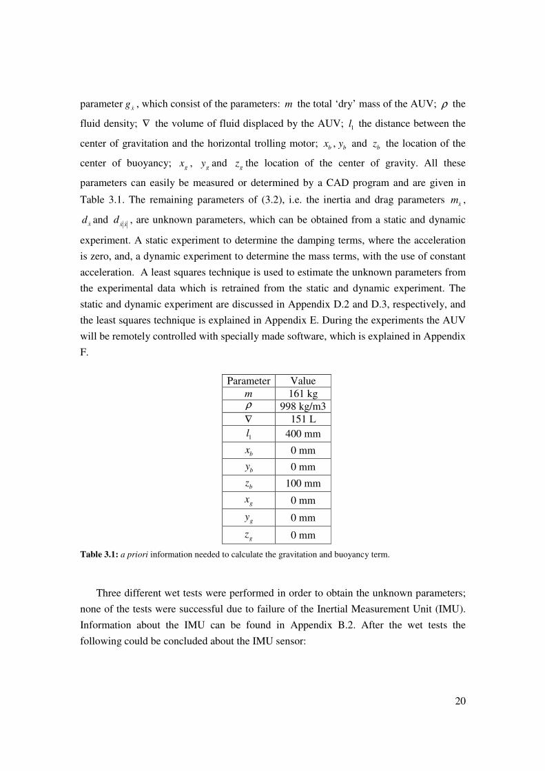
Appendix D.1. A priori information is used to calculate the gravitation and buoyancy

20

parameterxg & , which consist of the parameters: m the total ‘dry’ mass of the AUV; ρ the

fluid density; ∇ the volume of fluid displaced by the AUV; 1l the distance between the

center of gravitation and the horizontal trolling motor; bx , by and bz the location of the

center of buoyancy; gx , gy and gz the location of the center of gravity. All these

parameters can easily be measured or determined by a CAD program and are given in

Table 3.1. The remaining parameters of (3.2), i.e. the inertia and drag parameters xm& ,

xd & and x x

d& & , are unknown parameters, which can be obtained from a static and dynamic

experiment. A static experiment to determine the damping terms, where the acceleration

is zero, and, a dynamic experiment to determine the mass terms, with the use of constant

acceleration. A least squares technique is used to estimate the unknown parameters from

the experimental data which is retrained from the static and dynamic experiment. The

static and dynamic experiment are discussed in Appendix D.2 and D.3, respectively, and

the least squares technique is explained in Appendix E. During the experiments the AUV

will be remotely controlled with specially made software, which is explained in Appendix

F.

Parameter Value

m 161 kg ρ 998 kg/m3

∇ 151 L

1l 400 mm

bx 0 mm

by 0 mm

bz 100 mm

gx 0 mm

gy 0 mm

gz 0 mm

Table 3.1: a priori information needed to calculate the gravitation and buoyancy term.

Three different wet tests were performed in order to obtain the unknown parameters;

none of the tests were successful due to failure of the Inertial Measurement Unit (IMU).

Information about the IMU can be found in Appendix B.2. After the wet tests the

following could be concluded about the IMU sensor:

21

1. The magnetometer of the IMU is disrupted by the magnetic field created by the

other electronic components. Instead of measuring the earths magnetic field as

reference frame the IMU started measuring the magnetic field of the electronic

equipment as reference frame, which led to an inaccurate orientation matrix.

Relocating the IMU within the hull of the AUV did not solve this problem.

2. The accelerometers within the IMU are not accurate enough to determine the

velocity of the AUV. The noise level is too high and the bias stability is to low for

measuring the velocity and position of the AUV correctly. Note that the errors in

the acceleration measurement are integrated into progressively larger errors in

velocity.

Due to the IMU failure the system identification approach with the use of a static and

dynamic experiment can not be completed successfully, since the velocity of the AUV is

unknown.

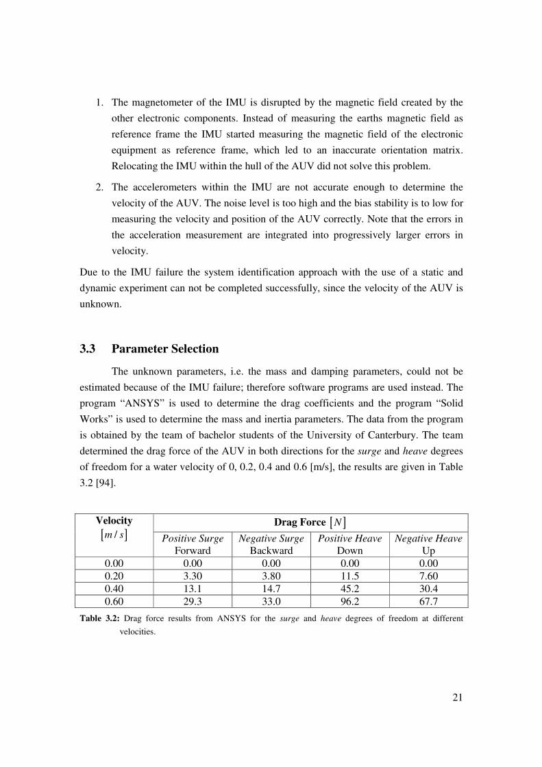
3.3 Parameter Selection

The unknown parameters, i.e. the mass and damping parameters, could not be

estimated because of the IMU failure; therefore software programs are used instead. The

program “ANSYS” is used to determine the drag coefficients and the program “Solid

Works” is used to determine the mass and inertia parameters. The data from the program

is obtained by the team of bachelor students of the University of Canterbury. The team

determined the drag force of the AUV in both directions for the surge and heave degrees

of freedom for a water velocity of 0, 0.2, 0.4 and 0.6 [m/s], the results are given in Table

3.2 [94].

Drag Force [ ]N Velocity

[ ]/m s Positive Surge

Forward

Negative Surge

Backward

Positive Heave

Down

Negative Heave

Up

0.00 0.00 0.00 0.00 0.00

0.20 3.30 3.80 11.5 7.60

0.40 13.1 14.7 45.2 30.4

0.60 29.3 33.0 96.2 67.7

Table 3.2: Drag force results from ANSYS for the surge and heave degrees of freedom at different

velocities.

22

The drag force results obtained by the team of bachelor students are analyzed by

the author. First a quadratic fit of the data is made with the program Matlab, which

estimates the unknown terms of the drag force equation

2

1 2 3dF p v p v p= + + (3.3),

where dF denotes the drag force, v the velocity, p1 the quadratic drag term, p2 the linear

drag term and p3 the equation offset for basic fitting. The parameters are found by the

basic fitting option of Matlab and are given in Table 3.3. The data points obtained and the

quadratic fitting are shown in Figure 3.4. Note that the quadratic fitting goes through all

data points because the data points were calculated with a quadratic solver in ANSYS.

Later on the obtained drag terms will be compared with other AUV’s to see if the

analysis with ANSYS made sense.

Quadratic Fit

Parameter

Positive Surge

Forward

Negative Surge

Backward

Positive Heave

Down

Negative Heave

Up

p1 80.625 90.625 246.88 185.63

p2 0.475 0.575 13.025 1.575

p3 -0.005 0.015 -0.245 -0.035

Table 3.3: Quadratic fitting parameters, for drag force data fitting in surge and heave degrees of freedom.

0 0.1 0.2 0.3 0.4 0.5 0.60

10

20

Dra

g f

orc

e [

N]

Positive Surge

quadratic fitting

data points

0 0.1 0.2 0.3 0.4 0.5 0.60

10

20

30

Negative Surge

0 0.1 0.2 0.3 0.4 0.5 0.60

20

40

60

80

Positive Heave

Velocity [m/s]

Dra

g f

orc

e [

N]

0 0.1 0.2 0.3 0.4 0.5 0.60

20

40

60

Negative Heave

Velocity [m/s]

Figure 3.4: Quadratic fitting of the obtained drag force data, velocity versus drag force, for both directions

of the surge and heave degrees of freedom.

The mass and inertia parameters are obtained with the program Solid Works. The

complete AUV is built in Solid Works by the team of bachelor students and they were

23

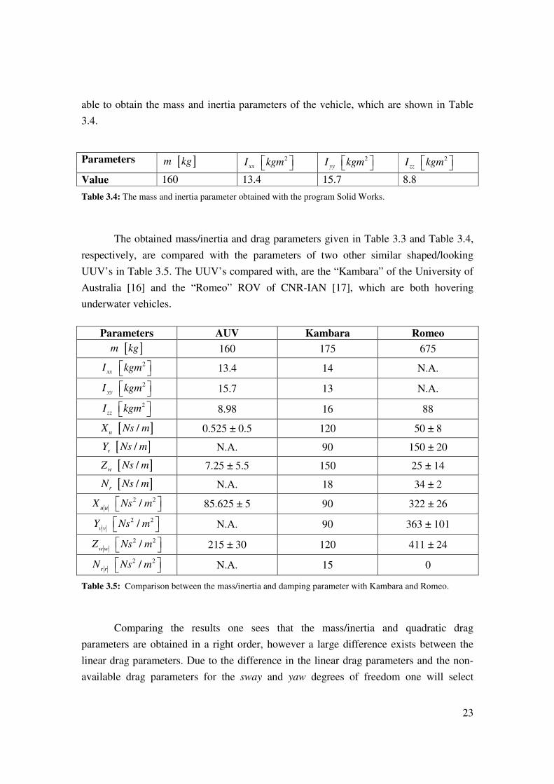
able to obtain the mass and inertia parameters of the vehicle, which are shown in Table

3.4.

Parameters m [ ]kg xxI 2kgm yyI 2kgm zzI 2kgm

Value 160 13.4 15.7 8.8

Table 3.4: The mass and inertia parameter obtained with the program Solid Works.

The obtained mass/inertia and drag parameters given in Table 3.3 and Table 3.4,

respectively, are compared with the parameters of two other similar shaped/looking

UUV’s in Table 3.5. The UUV’s compared with, are the “Kambara” of the University of

Australia [16] and the “Romeo” ROV of CNR-IAN [17], which are both hovering

underwater vehicles.

Parameters AUV Kambara Romeo

m [ ]kg 160 175 675

xxI 2kgm 13.4 14 N.A.

yyI 2kgm 15.7 13 N.A.

zzI 2kgm 8.98 16 88

uX [ ]/Ns m 0.525 ± 0.5 120 50 ± 8

vY [ ]/Ns m N.A. 90 150 ± 20

wZ [ ]/Ns m 7.25 ± 5.5 150 25 ± 14

rN [ ]/Ns m N.A. 18 34 ± 2

u uX 2 2/Ns m 85.625 ± 5 90 322 ± 26

v vY 2 2/Ns m N.A. 90 363 ± 101

w wZ 2 2/Ns m 215 ± 30 120 411 ± 24

r rN 2 2/Ns m N.A. 15 0

Table 3.5: Comparison between the mass/inertia and damping parameter with Kambara and Romeo.

Comparing the results one sees that the mass/inertia and quadratic drag

parameters are obtained in a right order, however a large difference exists between the

linear drag parameters. Due to the difference in the linear drag parameters and the non-

available drag parameters for the sway and yaw degrees of freedom one will select

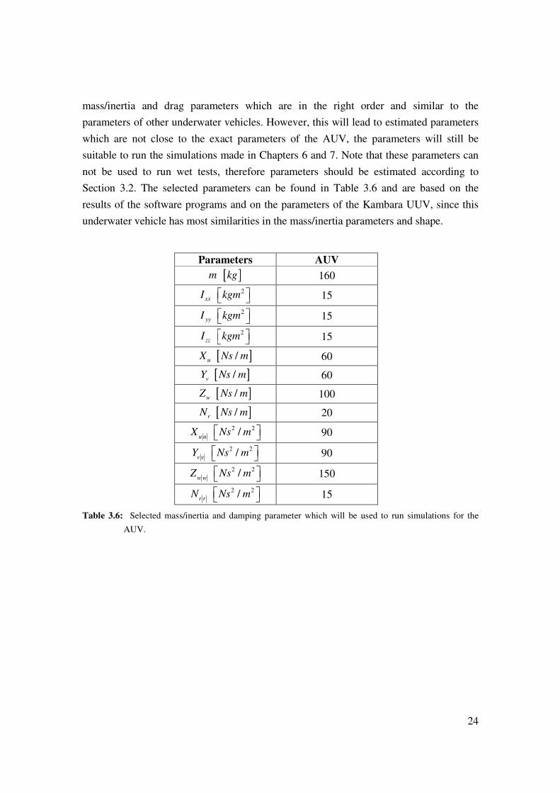
24

mass/inertia and drag parameters which are in the right order and similar to the

parameters of other underwater vehicles. However, this will lead to estimated parameters

which are not close to the exact parameters of the AUV, the parameters will still be

suitable to run the simulations made in Chapters 6 and 7. Note that these parameters can

not be used to run wet tests, therefore parameters should be estimated according to

Section 3.2. The selected parameters can be found in Table 3.6 and are based on the

results of the software programs and on the parameters of the Kambara UUV, since this

underwater vehicle has most similarities in the mass/inertia parameters and shape.

Parameters AUV

m [ ]kg 160

xxI 2kgm 15

yyI 2kgm 15

zzI 2kgm 15

uX [ ]/Ns m 60

vY [ ]/Ns m 60

wZ [ ]/Ns m 100

rN [ ]/Ns m 20

u uX 2 2/Ns m 90

v vY 2 2/Ns m 90

w wZ 2 2/Ns m 150

r rN 2 2/Ns m 15

Table 3.6: Selected mass/inertia and damping parameter which will be used to run simulations for the

AUV.

25

Chapter 4

Control of AUVs

The control of AUVs presents several difficulties caused by the nonlinear dynamics of

the vehicle and model uncertainties. It is important to explore different controllers that

have been implemented on AUVs. Therefore, problems of controlling AUVs and control

techniques are discussed in Section 4.1. A feedback linearizing control technique is

chosen to design control laws for control in the surge, heave and yaw degrees of freedom.

The feedback linearizing control technique is derived and discussed in Section 4.2. In the

x-y plane the AUV is only actuated in the surge and yaw degrees of freedom caused by

the trolling motor configuration. An under-actuated control problem arises since the

AUV, in the x-y plane, is able to move in three directions ( ), ,x y ψ . To steer the AUV

with a smooth motion from an initial position A to a different position B, in the x-y plane,

a path planning model is derived in Section 4.3.

4.1 Control Problems

Complex nonlinear forces acting upon an underwater vehicle, especially with

open frame AUVs, make the control more tricky, which has been explained in Chapters 2

and 3. Several complex nonlinear forces are, for example, hydrodynamic drag, lift forces,

Coriolis and centripetal forces, gravity and buoyancy forces, thruster forces, and

environmental disturbances [17]. These forces are not added to the equation of motion in

the complex form: some are simplified and others are left out. Assumptions and

simplifications made to the dynamics have been explained in Chapter 3. Control gets

26

even more complicated due to the difficulties in observing and measuring the AUV’s

response in the water [18].

Many universities and companies have interest in developing control techniques

for underwater vehicles with the aim to improve the dynamic response of underwater

vehicles. A great amount of research work on the design and implementation of different

controllers is already available. A few control techniques used for underwater vehicles

control are explained in Appendix H, the explanation includes PID Control, Linear

Quadratic Gaussian Control, Fuzzy Logic Control, Adaptive Control and Sliding Mode

Control.

4.2 Feedback Linearization

A common approach used in controlling nonlinear systems is feedback

linearization. The basic idea of the approach is to transform, if possible, the nonlinear

system into a linear system via a change of variables and/or a suitable control input and

then use a linear control technique to stabilize the linear system. The feedback

linearization approach requires full state measurement and according to J.E.Slotine and

W.Li [73] is used to solve a number of practical nonlinear control problems. However, it

should be noted that in combination with parameter uncertainty and/or disturbances does

not always guarantee a robust system.

Control of the one degree of freedom dynamical model via feedback linearization

is derived in subsection 4.2.1. The nonlinear model is transformed into a linear model

which is stabilized with a PD controller. Afterwards in subsection 4.2.2 the control law is

extended to a tracking controller and the PD controller is changed into a PID controller

for better robustness to account for parameter perturbations. The tracking controller is

implemented in Matlab Simulink and simulations are run in section 4.2.3.

4.2.1 Derivation of the Feedback Linearization

The one degree of freedom dynamical model

x x x xx xm x d x d x x gτ= − − −& & & && &

&& & & & (4.1)

derived in Chapter 3 can be rewritten as

xx ax bx x c dτ= − − − + &&& & & & (4.2),

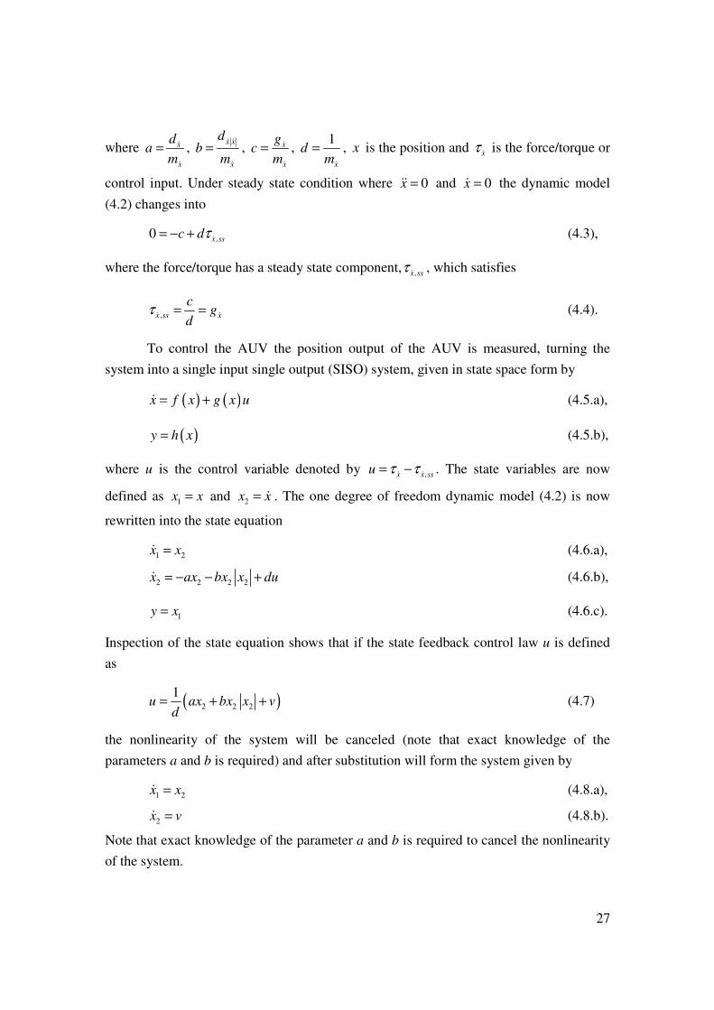
27

where x

x

da

m= &

&

, x x

x

db

m=

& &

&

, x

x

gc

m= &

&

, 1

x

dm

=&

, x is the position and xτ & is the force/torque or

control input. Under steady state condition where 0x =&& and 0x =& the dynamic model

(4.2) changes into

,0 x ssc dτ= − + & (4.3),

where the force/torque has a steady state component,,x ss

τ & , which satisfies

,x ss x

cg

dτ = =& & (4.4).

To control the AUV the position output of the AUV is measured, turning the

system into a single input single output (SISO) system, given in state space form by

( ) ( )x f x g x u= +& (4.5.a),

( )y h x= (4.5.b),

where u is the control variable denoted by ,x x ssu τ τ= −& & . The state variables are now

defined as 1x x= and 2x x= & . The one degree of freedom dynamic model (4.2) is now

rewritten into the state equation

1 2x x=& (4.6.a),

2 2 2 2x ax bx x du= − − +& (4.6.b),

1y x= (4.6.c).

Inspection of the state equation shows that if the state feedback control law u is defined

as

( )2 2 2

1u ax bx x v

d= + + (4.7)

the nonlinearity of the system will be canceled (note that exact knowledge of the

parameters a and b is required) and after substitution will form the system given by

1 2x x=& (4.8.a),

2x v=& (4.8.b).

Note that exact knowledge of the parameter a and b is required to cancel the nonlinearity

of the system.

28

This choice of u can be confirmed by the input-output linearization of the state

equation (4.6), which is given in Appendix G.1. After the implementation of the state

feedback control law the state equation is linearized to

x Ax Bv= +& (4.9),

where 0 1

0 0A

=

and 0

1B

=

. Now the linear state feedback control v Kx= − is

introduced to the nonlinear system, where [ ]1 2K k k= , which changes the linear state

equation into

( )x A BK x= −& (4.10).

The linear state feedback control v Kx= − has now to be designed such that ( )A BK− is

Hurwitz in order to have an asymptotically stable system, which means that all the

eigenvalues have to satisfy ( )Re 0iλ < . ( )A BK− is Hurwitz for 1 0k > and 2 0k > ,

which is verified in Appendix G.4.

The overall feedback control law xτ & , can now be derived with the use of the

linear state feedback control v, the state feedback control law u and the steady state

component ,x ssτ & , which results in

( ), 2 2 2 1 1 2 2

1x x ssu ax bx x c k x k x

dτ τ= + = + + − −& & (4.11),

where ( )2 2 2

1u ax bx x v

d= + + , 1 1 2 2v k x k x= − − and

,x ss

c

dτ =& . The overall state feedback

control law xτ & , is written down in the original coordinates in

1 2x x x x xx xd x d x x g m k x m k xτ = + + − −& & & & && &

& & & & (4.12)

and changes the systems dynamics into

2 1 0x k x k x+ + =&& & (4.13).

The overall state feedback control law is also known as computed torque control law. A

thumb rule in computed torque control is to choose 1k as 2k and 2k as 2k [73]. The

system dynamics (4.13) are hereby changed into

22 0x kx k x+ + =&& & (4.14).

Mind that k has to be larger than zero for stable closed loop dynamics.

29

4.2.2 Tracking

If the AUV needs to follow a certain trajectory then the control law xτ & needs to be

extended, so that the output y tracks a reference signal r(t). The error between the output

and the reference signal is called the tracking error e and is defined together with its

derivatives by

e x r= − (4.15.a),

e x r= −& & & (4.15.b),

e x r= −&& && && (4.15.c).

The tracking control law can be derived by taking 1 1e x r= − and 2 2e x r= − & , which gives

the state equation

1 2e e=& (4.16.a),

2 2 2 2e ax bx x du r= − − + −& && (4.16.b).

It is clear the state feedback control law u will now have to take the form

( )2 2 2 1 1 2 2

1u ax bx x r k e k e

d= + + − −&& (4.17),

which results in the overall state feedback control law

( )2 2 2 1 1 2 2

1x ax bx x c r k e k e

dτ = + + + − −& && (4.18).

The tracking control law which is the overall state feedback control law in original

coordinates is given by

1 2x x x x x xx xd x d x x g m r m k e m k eτ = + + + − −& & & & & && &

& & & && & (4.19),

with 1k = 2k and

2k = 2k . Note that this tracking control law requires the reference signals

, ,r r r& && to be available on-line at any time. When this is not possible during experiments,

due to a shortcoming of measurement equipment, the control law should be extended

with an observer in order to estimate unmeasured states. The system dynamics are now

reduces to the error dynamics (the tracking error of the closed loop system)

22 0e ke k e+ + =&& & (4.20).

Note that the error dynamics are formed by the substitution of the error equation (4.15.c)

and the tracking control law (4.19) into the system dynamics (4.1). If k is chosen positive

30

the error dynamics (4.20) will be stable and the error will go to zero, assuming that the

dynamic model is accurate. However the model parameters of the AUV are not known

exactly and the system dynamics are simplified, which means that the system can still

behave unacceptable.

An integral term is added to the linear feedback controller v in order to cope with

parameter perturbations. A parameter perturbation is caused, for example, by a

reconfiguration on the AUV, for instance a change of mass. Integrating the error between

the output and the reference signal will compensate the steady state error created by the

perturbed parameters.

An integral gain ik determines the magnitude of contribution of the integral term

to the tracking controllerxτ & . The integral term is described as

ik e∫ and is added to the

linear feedback controller v, which can be seen in

1 2 iv k e k e k e= − − − ∫& (4.21)

Note that this linear feedback controller is also known as a PID controller, where 1k

forms the proportional gain, ik the integral gain and 2k the derivative gain. More

information about PID control can be found in Appendix H.1. The tracking control law in

combination with the PID controller is now given in

1 2x x x x x x x ix x

d x d x x g m r m k e m k e m k eτ = + + + − − − ∫& & & & & & && && & & && & (4.22)

and the error dynamics can now be described by

22 0ie ke k e k e+ + + =∫&& & (4.23).

4.2.3 Simulation Results

Simulations will be run in Matlab Simulink to test the tracking control law

defined in (4.22). To be able to run a simulation a reference and plant model are made.

The reference model defines a reference trajectory for the AUV to follow. Note that the

reference signals , r r& and r&& need to be available online. The plant model will replace the

real AUV and represent the AUV dynamics. A more extensive explanation of the

implementation of the tracking control laws into Matlab Simulink is given in Appendix

K.

31

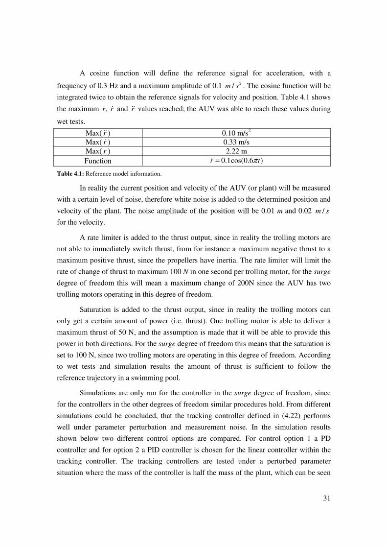
A cosine function will define the reference signal for acceleration, with a

frequency of 0.3 Hz and a maximum amplitude of 0.1 2/m s . The cosine function will be

integrated twice to obtain the reference signals for velocity and position. Table 4.1 shows

the maximum , r r& and r&& values reached; the AUV was able to reach these values during

wet tests.

Max( r&&) 0.10 m/s2

Max( r& ) 0.33 m/s

Max( r ) 2.22 m

Function 0.1cos(0.6 )r tπ=&&

Table 4.1: Reference model information.

In reality the current position and velocity of the AUV (or plant) will be measured

with a certain level of noise, therefore white noise is added to the determined position and

velocity of the plant. The noise amplitude of the position will be 0.01 m and 0.02 /m s

for the velocity.

A rate limiter is added to the thrust output, since in reality the trolling motors are

not able to immediately switch thrust, from for instance a maximum negative thrust to a

maximum positive thrust, since the propellers have inertia. The rate limiter will limit the

rate of change of thrust to maximum 100 N in one second per trolling motor, for the surge

degree of freedom this will mean a maximum change of 200N since the AUV has two

trolling motors operating in this degree of freedom.

Saturation is added to the thrust output, since in reality the trolling motors can

only get a certain amount of power (i.e. thrust). One trolling motor is able to deliver a

maximum thrust of 50 N, and the assumption is made that it will be able to provide this

power in both directions. For the surge degree of freedom this means that the saturation is

set to 100 N, since two trolling motors are operating in this degree of freedom. According

to wet tests and simulation results the amount of thrust is sufficient to follow the

reference trajectory in a swimming pool.

Simulations are only run for the controller in the surge degree of freedom, since

for the controllers in the other degrees of freedom similar procedures hold. From different

simulations could be concluded, that the tracking controller defined in (4.22) performs

well under parameter perturbation and measurement noise. In the simulation results

shown below two different control options are compared. For control option 1 a PD

controller and for option 2 a PID controller is chosen for the linear controller within the

tracking controller. The tracking controllers are tested under a perturbed parameter

situation where the mass of the controller is half the mass of the plant, which can be seen

32

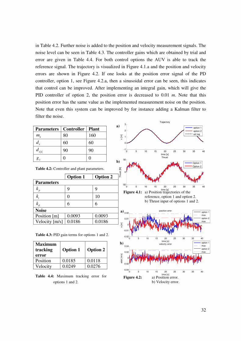
in Table 4.2. Further noise is added to the position and velocity measurement signals. The

noise level can be seen in Table 4.3. The controller gains which are obtained by trial and

error are given in Table 4.4. For both control options the AUV is able to track the

reference signal. The trajectory is visualized in Figure 4.1.a and the position and velocity

errors are shown in Figure 4.2. If one looks at the position error signal of the PD

controller, option 1, see Figure 4.2.a, then a sinusoidal error can be seen, this indicates

that control can be improved. After implementing an integral gain, which will give the

PID controller of option 2, the position error is decreased to 0.01 m. Note that this

position error has the same value as the implemented measurement noise on the position.

Note that even this system can be improved by for instance adding a Kalman filter to

filter the noise.

Table 4.2: Controller and plant parameters.

Table 4.3: PID gain terms for options 1 and 2.

Table 4.4: Maximum tracking error for

options 1 and 2.

Parameters Controller Plant

xm& 80 160

xd & 60 60

x xd & &

90 90

xg & 0 0

Option 1 Option 2

Parameters

pk 9 9

ik 0 10

dk 6 6

Noise

Position [m] 0.0093 0.0093

Velocity [m/s] 0.0186 0.0186

Maximum

tracking

error

Option 1 Option 2

Position 0.0185 0.0118

Velocity 0.0249 0.0276

Figure 4.2: a) Position error.

b) Velocity error.

Figure 4.1: a) Position trajectories of the

reference, option 1 and option 2.

b) Thrust input of options 1 and 2.

0 5 10 15 20 25 30 35 40-1

0

1

2

3

time [s]

x [

m]

Trajectory

option 1

option 2

ref traj

0 5 10 15 20 25 30 35 40-50

0

50

time [s]

Thru

st

[N]

Thrust

Option 1

Option 2

0 5 10 15 20 25 30 35 40-0.02

-0.01

0

0.01

0.02

time [s]

e [

m]

position error

option 1

max

option 2

max

0 5 10 15 20 25 30 35 40-0.04

-0.02

0

0.02

0.04

time [s]

edot

[m/s

]

velocity error

option 1

max

option 2

max

a)

b)

a)

b)

33

Next to the simulations described above other different simulations are run these are

described in Appendix I. The subject of these simulations and there appendices are listed

below:

- The effect of a high gain PD controller for the linear controller within the tracking

controller without noise and perturbation is described in Appendix I.1.

- The effect of perturbed parameters on low gain P control and high gain PD

control for the linear controller within the tracking controller is described in

Appendix I.2.

- The effect of the implementation of noise on low gain P control and high gain PD

control for the linear controller within the tracking controller is described in

Appendix I.3.

- The effect of the thrust rate limiter on high gain PD control for the linear

controller within the tracking controller is described in Appendix I.4.

- The effect of extreme parameter perturbation on the tracking controller which had

a PID controller for the linear controller within the tracking controller is described

in Appendix I.5.

The tracking controller defined in (4.22) with the PID gains given in Table 4.3 is able to

control the AUV in one degree of freedom and will track a position reference trajectory

with a maximum position error of 0.012 m. The tracking controller is optimized to

perform in the surge degree of freedom but a similar method can be applied for the heave

and yaw degrees of freedom. After doing so the AUV will be able to move controlled in

these degrees of freedom, but the AUV is still not able to move from an initial position A

to a different position B. Therefore path planning equations are needed, to define

reference signals for the surge, heave and yaw degrees of freedom.

4.3 Path Planning

With the controllers for the surge, heave and yaw degrees of freedom working, it

is time for the AUV to move from an initial position, named set-point A, to another

position, named set-point B, which has a different x, y, z and/or yaw position in the earth

fixed frame. The AUV is only able to move in the surge, heave and yaw degrees of

freedom, since only these degrees of freedom are controlled. An under-actuated problem

arises in the x-y plane because the AUV is unable to move in the sway direction. Take for

instance the relative positions A and B given in Figure 4.16. Note that set-point B has a

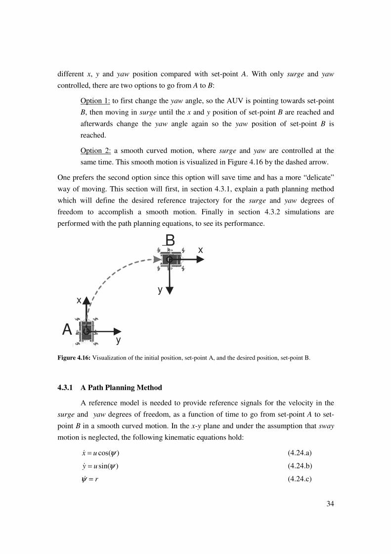
34

different x, y and yaw position compared with set-point A. With only surge and yaw

controlled, there are two options to go from A to B:

Option 1: to first change the yaw angle, so the AUV is pointing towards set-point

B, then moving in surge until the x and y position of set-point B are reached and

afterwards change the yaw angle again so the yaw position of set-point B is

reached.

Option 2: a smooth curved motion, where surge and yaw are controlled at the

same time. This smooth motion is visualized in Figure 4.16 by the dashed arrow.

One prefers the second option since this option will save time and has a more “delicate”

way of moving. This section will first, in section 4.3.1, explain a path planning method

which will define the desired reference trajectory for the surge and yaw degrees of

freedom to accomplish a smooth motion. Finally in section 4.3.2 simulations are

performed with the path planning equations, to see its performance.

A

B

x

y

y

x

Figure 4.16: Visualization of the initial position, set-point A, and the desired position, set-point B.

4.3.1 A Path Planning Method

A reference model is needed to provide reference signals for the velocity in the

surge and yaw degrees of freedom, as a function of time to go from set-point A to set-

point B in a smooth curved motion. In the x-y plane and under the assumption that sway

motion is neglected, the following kinematic equations hold:

cos( )x u ψ=& (4.24.a)

sin( )y u ψ=& (4.24.b)

rψ =& (4.24.c)

35

Inspired by M.Aicardi, G.Casalino, et.al. [78] the kinematic equations are rewritten into

polar coordinates given by

cos( )e u α= −& (4.25.a),

sin( )u

re

α α= − +& (4.25.b),

sin( )u

eβ α=& (4.25.c),

where e describes the error distance between the centers of gravity of the AUV in set-

point A and B, β describes the current orientation of the AUV with respect to the body

fixed frame of a virtual AUV in set-point B and α describes the angle between the

principal axis of the AUV and the distance error vector e. A visual representation for

better understanding of these parameters is given in Figure 4.17 where e describes the

error distance vector, and, α and β describe the alignment error vector. Note that the

kinematic equations given by the polar coordinates are only valid for 0e > and that the

kinematic equations are only valid for non zero values since α and β are undefined

when e = 0. The system and its kinematic equations given in (4.25) will, from now on,

simply be named “the P-system”.

A

B

α

β

ψx

y

y

x

e

u

u

Figure 4.17: Visualization of the polar coordinate parameters e, α and β .

To fulfill option 2 defined above suitable chosen control laws for u and r need to guide

the P-system asymptotically towards the limiting point [ ] [ ], , 0,0,0e α β = , without

36

reaching the condition e = 0. Lyapunov’s stability theorem is used to derive control laws

for u and r which asymptotically stabilize the system.

Lyapunov theory suggests that when the energy of a system keeps decreasing it

will finally arrive at a stable equilibrium point, or in other words, if the derivative of the

energy function of a certain system remains smaller than zero at any time, the system will

be asymptotically stable. Lyapunov found out that this also works for other functions

rather than energy functions, which led to Lyapunov’s stability theorem [74], see

Appendix G.5.

A proper Lyapunov candidate function for the P-system is given by

( )2 2 20.5V e α β= + + (4.26),

which is in positive definite quadratic form, lower bounded and satisfies (0) 0V = and

( ) 0V x > in { }0D − . Note that the Lyapunov candidate function can be separated into

2

1 0.5V e= and ( )2 2

2 0.5V α β= + , which represent the Lyapunov candidate function for

the error distance vector and the alignment vector, respectively.

The derivative of the Lyapunov candidate function is given by

1 2V V V ee αα ββ= + = + + && & & && (4.28),

where the derivatives of its separates are

1 cos( )V eu α= −& (4.29),

2 sin( ) sin( )u u

V re e

α α β α

= − + +

& (4.30).

One needs to design a control law for u and r in such a way that the derivative of the

Lyapunov’s candidate function, V& , is always smaller than zero (see Appendix G.5). Note

that in case of e = 0 the Lyapunov candidate function is not well defined. However, when

one defines the control law u as

1 cos( )u k e α= (4.31),

with 1 0k > than 1V& becomes negative semi definite. Since V is lower bounded by zero

and is non increasing in time ( 1 0V ≤& ) 1V will asymptotically converge towards a non

negative finite limit. After implementation of the control law u the derivative of the

Lyapunov candidate functions 1V& and 2V& become

37

2 2

1 1 1cos( ) cos ( ) 0, 0V eu k e kα α= − = − ≤ >& (4.32),

and

( )2 1 1cos( )sin( ) cos( )sin( )V r k kα α α β α α= − + +& (4.32),

respectively.

After the implementation of the control law r given by

1 1 2cos( )sin( ) cos( )sin( )r k k kβ

α α α α αα

= + + (4.33),

with 2 0k > , 2V& becomes negative semi definite as can be seen in

2

2 2 20, 0V k kα= − ≤ >& (4.34)

The summation of 1V& and 2V& gives the derivative of the Lyapunov’s candidate function

2 2 2

1 2 1 2cos ( ) 0, 0, 0V k e k k kα α= − − ≤ > >& (4.35),

which is in a negative semi definite form. According to Barbalat’s lemma V& converges to

zero for increasing time [73], since V is lower bounded and V& is negative semi-definite

and uniformly continuous in time. Barbalat’s lemma is given in Appendix G.6 and for the

application of Barbalat’s lemma a “Lyapunov-Like” method is used, which is given in

Appendix G.7. Since V& converges to zero for increasing time and V& can only become

zero when e andα are zero the P-system will have to converge to the line

[ ] [ ], , 0,0,e α β β= . The substitution of ( , ) (0,0)e α = into the kinematic equations, with

the implementation of the control laws for u and r, given by

2

1 cos ( )e k e α=& (4.36.a)

1 2cos( )sin( )k kβ

α α α αα

= − −& (4.36.b)

1 cos( )sin( )kβ α α=& (4.36.c),

indicates that e& and β& also converge to zero. The convergence of β& to zero implies that

β goes to a finite limit, named β . Since β goes to a finite limit α& will converge to the

finite limit 1k β− , note that

0

cos( )sin( )lim 1α

α α

α→= . According to Barbalat’s lemma, see

Appendix G.6, α& converges to zero for increasing time since α& is a uniformly

continuous in time and α has a finite limit for increasing time. The convergence of α& to

38

zero implies that β will have to converge to zero, since α& can only be zero when all its

parameters are zero. Since β will also converge to zero it is proven that the P-system

will not only converge to the line [ ] [ ], , 0,0,e α β β= but towards the limiting point

[ ] [ ], , 0,0,0e α β = .

4.3.2 Simulation Results

The kinematic equation are written in polar coordinates, so only the relative

distance between set-point A and set-point B will matter. Set-point B will always

positioned at [ ] [ ], , 0,0,0e α β = , which means that the polar coordinate system will

always align with the body-fixed frame of the AUV in set-point B. Lets take, for

example, the following earth fixed coordinates for set-point A [ ] [ ], , 0,0,0x y ψ = and for

set-point B [ ] [ ], , 1,0,0x y ψ = , in polar coordinates the same distance would denote

[ ] [ ], , 1,0,0e α β = for set-point A and [ ] [ ], , 0,0,0e α β = for set-point B.

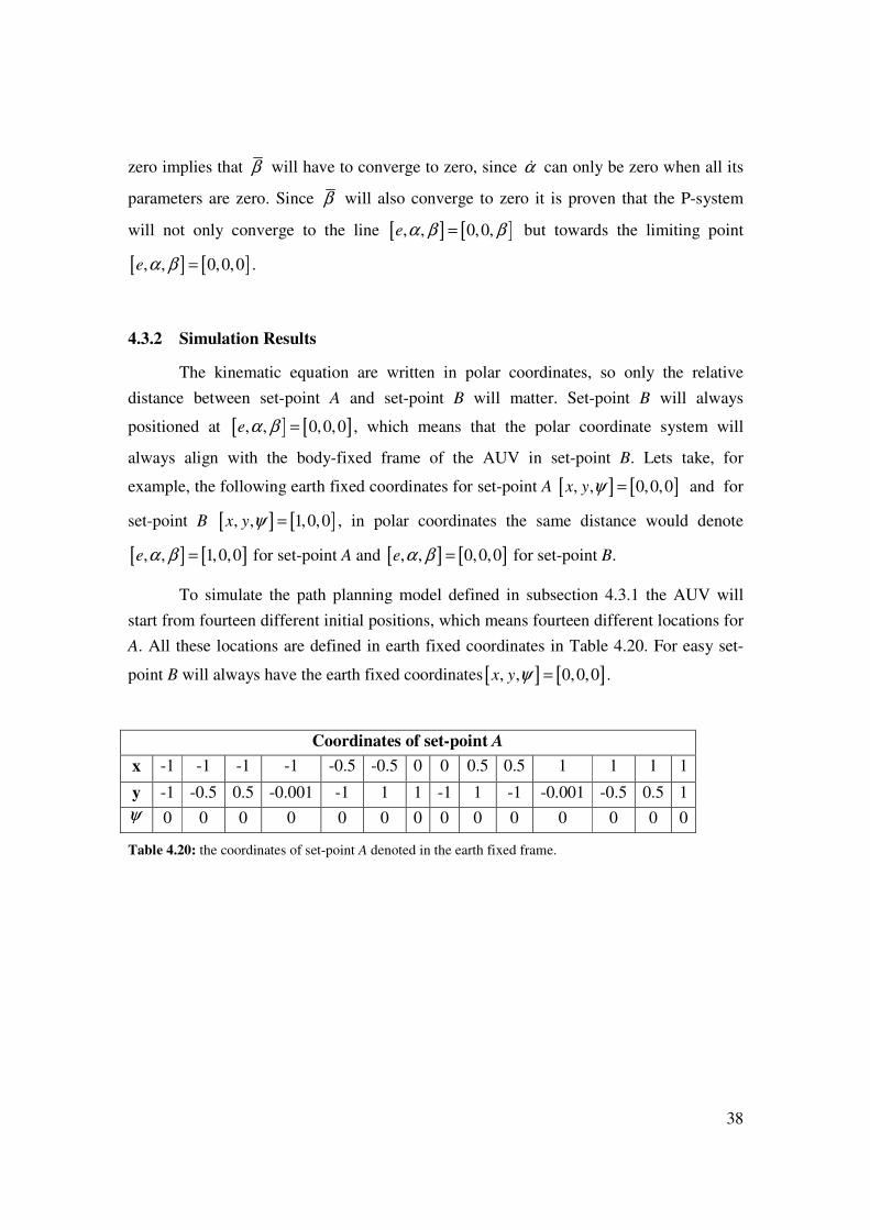
To simulate the path planning model defined in subsection 4.3.1 the AUV will

start from fourteen different initial positions, which means fourteen different locations for

A. All these locations are defined in earth fixed coordinates in Table 4.20. For easy set-

point B will always have the earth fixed coordinates[ ] [ ], , 0,0,0x y ψ = .

Coordinates of set-point A

x -1 -1 -1 -1 -0.5 -0.5 0 0 0.5 0.5 1 1 1 1

y -1 -0.5 0.5 -0.001 -1 1 1 -1 1 -1 -0.001 -0.5 0.5 1

ψ 0 0 0 0 0 0 0 0 0 0 0 0 0 0

Table 4.20: the coordinates of set-point A denoted in the earth fixed frame.

39

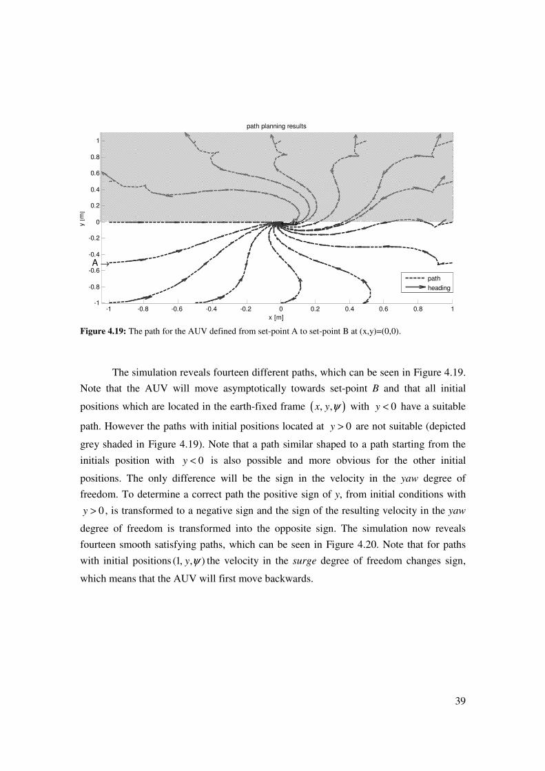
Figure 4.19: The path for the AUV defined from set-point A to set-point B at (x,y)=(0,0).

The simulation reveals fourteen different paths, which can be seen in Figure 4.19.

Note that the AUV will move asymptotically towards set-point B and that all initial

positions which are located in the earth-fixed frame ( ), ,x y ψ with 0y < have a suitable

path. However the paths with initial positions located at 0y > are not suitable (depicted

grey shaded in Figure 4.19). Note that a path similar shaped to a path starting from the

initials position with 0y < is also possible and more obvious for the other initial

positions. The only difference will be the sign in the velocity in the yaw degree of

freedom. To determine a correct path the positive sign of y, from initial conditions with

0y > , is transformed to a negative sign and the sign of the resulting velocity in the yaw

degree of freedom is transformed into the opposite sign. The simulation now reveals

fourteen smooth satisfying paths, which can be seen in Figure 4.20. Note that for paths

with initial positions (1, , )y ψ the velocity in the surge degree of freedom changes sign,

which means that the AUV will first move backwards.

-1 -0.8 -0.6 -0.4 -0.2 0 0.2 0.4 0.6 0.8 1-1

-0.8

-0.6

-0.4

-0.2

0

0.2

0.4

0.6

0.8

1

x [m]

y [

m]

path planning results

← B

A →

path

heading

40

-1 -0.8 -0.6 -0.4 -0.2 0 0.2 0.4 0.6 0.8 1-1

-0.8

-0.6

-0.4

-0.2

0

0.2

0.4

0.6

0.8

1

x [m]

y [

m]


← B

A →

path

heading

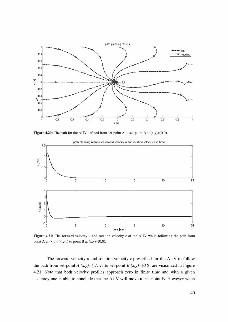
Figure 4.20: The path for the AUV defined from set-point A to set-point B at (x,y)=(0,0).

0 5 10 15 20 250

0.5

1

1.5

u [

m/s

]

path planning results for forward velocity u and rotation velocity r vs time

0 5 10 15 20 25-1

0

1

2

3

4

time [sec]

r [r

ad/s

]

Figure 4.21: The forward velocity u and rotation velocity r of the AUV while following the path from

point A at (x,y)=(-1,-1) to point B at (x,y)=(0,0).

The forward velocity u and rotation velocity r prescribed for the AUV to follow

the path from set-point A (x,y)=(-1,-1) to set-point B (x,y)=(0,0) are visualized in Figure

4.21. Note that both velocity profiles approach zero in finite time and with a given

accuracy one is able to conclude that the AUV will move to set-point B. However when

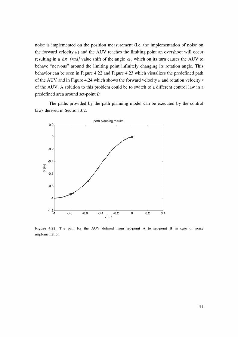
41

noise is implemented on the position measurement (i.e. the implementation of noise on

the forward velocity u) and the AUV reaches the limiting point an overshoot will occur

resulting in a kπ [rad] value shift of the angle α , which on its turn causes the AUV to

behave “nervous” around the limiting point infinitely changing its rotation angle. This

behavior can be seen in Figure 4.22 and Figure 4.23 which visualizes the predefined path

of the AUV and in Figure 4.24 which shows the forward velocity u and rotation velocity r

of the AUV. A solution to this problem could be to switch to a different control law in a

predefined area around set-point B.

The paths provided by the path planning model can be executed by the control

laws derived in Section 3.2.

-1 -0.8 -0.6 -0.4 -0.2 0 0.2 0.4-1.2

-1

-0.8

-0.6

-0.4

-0.2

0

0.2

x [m]

y [

m]


Figure 4.22: The path for the AUV defined from set-point A to set-point B in case of noise

implementation.

42

-6 -4 -2 0 2 4 6 8

x 10-3

-10

-8

-6

-4

-2

0

2

4

6

8

x 10-3

x [m]

y [

m]


Figure 4.23: The path for the AUV defined from set-point A to set-point B in case of noise

implementation.

0 5 10 15 20 25-0.5

0

0.5

1

1.5

u [

m/s

]

path planning results for forward velocity u and rotation velocity r vs time

0 5 10 15 20 25-20

-10

0

10

time [sec]

r [r

ad/s

]

Figure 4.24: The forward velocity u and rotation velocity r of the AUV while following the path from

point A at (x,y)=(-1,-1) to point B at (x,y)=(0,0) in case of noise implementation.

43

4.4 Summary

In the x-y plane the AUV is only able to move in the surge and yaw degrees of

freedom due to the trolling motor configuration. An under-actuated control problem

arises, since one is only able to control two degrees of freedom while the AUV is able to

move in three degrees of freedom. To steer the AUV with a smooth motion from an

initial position A to a different position B, in the x-y plane, a path planning model is

derived. The path planning model describes a path from A to B with the use of polar

coordinates which the AUV is able to follow controlling only the surge and yaw degrees

of freedom. The assumption is made that sway-motion of the AUV can be neglected.

Simulations with the model reveal that the path planning works correct, except for

planning a straight line due to singularity reasons. This problem can be solved by

introducing a switching controller which is able to switch between different path planning

models.

A feedback linearizing controller extended to a tracking controller is designed in

order to track a reference trajectory in one degree of freedom. The reference trajectory

can be provided by the path planning model, however a separate feedback linearizing

controller is needed for the surge, heave and yaw degrees of freedom. The feedback

linearizing control technique changes the nonlinear dynamical system into a linear system

through a suitable chosen control input. The linear system is stabilized with the use of

PID control. In simulations the controller performed well under parameter perturbation

and the implementation of noise on the feedback position and velocity signals of the

plant. It should be noted that all states need to be available online to control the AUV.

When during experiments full state measurement is not possible then the control law

should be extended with an observer in order to estimate unmeasured states.

45

Chapter 5

Tracking control of an under-actuated AUV

In this chapter a state feedback control technique is proposed to control the AUV in an

under-actuated situation, where motion in sway is no longer neglected. Section 5.1 will

explain the control technique and section 5.2 will show simulation results.

5.1 An Under-Actuated AUV

The AUV is able to follow a predefined path in 3D space by enabling different

trolling motors. The setup of the trolling motors makes it possible to control all degrees

of freedom except for the sway direction. No trolling motors are aligned in the sway

direction, so there is no sway control force. The roll and pitch degrees of freedom are

stabilized by the aligning moment of buoyancy and gravity and are therefore not

controlled. This means that one is able to control the surge, heave and yaw degrees of

freedom, where an error in the sway direction can only be adjusted by surge and yaw

control.

The control laws for the surge and yaw degrees of freedom need to control three

degrees of freedom, which means that one is dealing with an under-actuated problem.

Motion in heave is neglected in this situation, since the under-actuated problem only

concerns the surge, sway and yaw degrees of freedom. In this section control laws for the

surge and yaw degrees of freedom will be derived, these control laws are different from

control laws derived in Chapter 4. The idea is to derive new control laws is such way that

the controlled system is able to follow a path in the x-y plane and an error in sway is

corrected by controlling the system in the surge and yaw direction. The assumptions

made in Chapter 4 apply to this problem, only the motion in the sway direction and the

46

Coriolis and Centripetal Matrix are not neglected anymore. Note that when the AUV is

making a curve and is able to move in sway the control laws will need to take in

consideration the Coriolis and Centripetal forces will try to “push” the vehicle out of

track.

The dynamics of the AUV in the surge, sway and yaw degrees of freedom are

defined in matrix form by

( )Jη η ν=& & (5.1)

( ) ( )M C Dν ν ν ν ν τ= − − +& (5.2),

which follow directly from the dynamic model (2.8) for 6 degrees of freedom. Under the

modeling assumptions made in Section 3.1 the matrix form of the AUV dynamics is

rewritten into

( ) ( )x uC vSψ ψ= −& (5.3.a)

( ) ( )y uS vCψ ψ= +& (5.3.b)

rψ =& (5.3.c)

11 22 11 um u m vr d u τ= − +& (5.3.d)

22 11 22m v m ur d v= − −& (5.3.e)

( )33 11 22 33 rm r m m uv d r τ= − − +& (5.3.f)

Where [ ]T

u v rν = , [ ]T

x yη ψ= , 11 22 33( , , )M diag m m m= ,

11 22 33( ) ( , , )D diag d d dν = , [ ]0T

u rτ τ τ= ,

( ) ( ) 0

( ) ( ) ( ) 0

0 0 1

C S

J S C

ψ ψ

η ψ ψ

− =

and

22

11

22 11

0 0

( ) 0 0

0

m v

C m u

m v m u

ν

− = −

.

Where x, y and ψ represent the position and orientation of the AUV in the earth-fixed

frame and u, v and r are the velocities in surge, sway and yaw respectively. The

parameters 11m , 22m and 33m represent the rigid body and added mass of the inertia and

mass of the AUV and 11d , 22d and 33d represent the linear damping terms of the AUV.

According to [92, 93] no pure state feedback control law exists to asymptotically

stabilize the system given in (5.3). This problem is solved by introducing time-variance

in the feedback law, an approach which is used for mobile robots in [80, 81], and is

47

extended to the control of ships in [83, 88, 89], and used for AUV’s with the use of

backstepping techniques in [82, 84, 85, 86, 87, 90, 91].

The position error between the current position of the AUV and a reference

position of a virtual AUV is given by

rx x− (5.4.a)

ry y− (5.4.b)

rψ ψ− (5.4.c),

which represents the position errors in the earth fixed frame. Where x , y and ψ

represent the current position of the AUV and rx , ry and rψ the reference position of a

virtual AUV. The problem with the position error proposed in (5.4) is that the error

depends on the initial position of the earth fixed frame. Lefeber [83] inspired by the work

of Pettersen and Egeland [93] solved this problem by a change of coordinates, which led

to the natural error coordinates given by

( ) ( ) 0

( ) ( ) 0

0 0 1

e r

e r

e r

x C S x x

y S C y y

ψ ψ

ψ ψ

ψ ψ ψ

− = − − −

(5.5)

The position errors (5.4) are now considered in the body fixed frame of the AUV, so the

tracking errors of the AUV can now be defined by

( ) ( )( ) ( )e r rx C x x S y yψ ψ= − + − (5.6.a),

( ) ( )( ) ( )e r ry S x x C y yψ ψ= − − + − (5.6.b),

e rψ ψ ψ= − (5.6.c),

e ru u u= − (5.6.d),

e rv v v= − (5.6.e),

e rr r r= − (5.6.f).

Where ru ,

rv , rr ,

rx , ry ,

rψ , ,u r

τ and ,r r

τ represent the reference coordinates which

have to satisfy

( ) ( )r r r r rx u C v Sψ ψ= −& (5.7.a),

( ) ( )r r r r ry u S v Cψ ψ= +& (5.7.b),

r rrψ =& (5.7.c),

48

11 22 11 ,r r r r u rm u m v r d u τ= − +& (5.7.d),

22 11 22r r r rm v m u r d v= − −& (5.7.e),

( )33 11 22 33 ,r r r r r rm r m m u v d r τ= − − +& (5.7.f).

Differentiating the tracking errors will lead to the tracking error dynamics, which are

given by

cos( ) sin( ) ( )e r e r e e e r ex u u v r y r t yψ ψ= − − + +& (5.8.a),

cos( ) sin( ) ( )e r e r e e e r ey v v u r x r t xψ ψ= − + − −& (5.8.b),

e erψ =& (5.8.c),

( ) ( )22 11,

11 11 11

1( )e e e e r r e e u u r

m du v r v r t v r u

m m mτ τ= + + − + −& (5.8.d),

( )11 22

22 22

( )e e e e r r e e

m dv u r u r t u r v

m m= − + + −& (5.8.e),

( )( )11 22 33

33 33 33

1e e e e r r e e r

m m dr u v u v u v r

m m mτ

−= + + − +& (5.8.f).

The goal now is to stabilize the tracking error dynamics with a suitable choice of

control laws for uτ in surge and

rτ in yaw in order to establish tracking control for the

AUV. From now on a state feedback approach proposed by Lefeber in [83] and Lefeber,

Pettersen and Nijmeijer in [88] is followed to asymptotically stabilize the tracking error

dynamics. In these papers a state-tracking problem for an under-actuated ship (with only

surge and yaw controlled) is solved by means of a global tracking controller. The author

is of the opinion that a clear explanation of this approach will form a decent basis for the

understanding of the underactuated control problem for the AUV, since the control law

proposed has a simple structure and guarantees global exponential stability of the

tracking error dynamics. From this basis further developments for the underactuated

control of the AUV can more easily be made in further research.

In [88] it is experimentally proven that the control law has a certain robustness

against modeling errors and disturbances due to currents and wave drift forces. The

control law can easily be transformed to a control law suitable for the AUV, since the

dynamical model of a ship and AUV are similar in the x-y plane.

A feedback control law for rτ , given by

( )( ), 11 22 33 33r r r r r em m uv u v d r mτ τ υ= − − − + + (5.9)

49

is proposed, which will change the tracking dynamics (5.8.c) and (5.8.f) into the linear

system given by

e erψ =& (5.10),

er υ=& (5.11),

respectively. The linear system can be stabilized by the linear control law given by

1 2 1 2, 0, 0e ek r k k kυ ψ= − − > >& (5.12),

which will change the control law for rτ into

( )( ), 11 22 1 2 1 33 2, , 0r r r r r e em m uv u v k r k k d kτ τ ψ= − − − − − > − >& (5.13)

and the tracking dynamics into

( )33 1 2

33 33

1 0e e

e e

d k kr r

m m

ψ ψ

= + − −

&

& (5.14)

Under the assumption that (5.14) is stabilized and that er and eψ go to zero, one is able

to rewrite the remaining error tracking dynamics, 5.8.a, 5.8.b, 5.8.d and 5.8.e, into

( )e e r ex u r t y= +& (5.15)

( )e e r ey v r t x= −& (5.16)

( )22 11,

11 11 11

1( )e e r e u u r

m du v r t u

m m mτ τ= − + −& (5.17)

11 22

22 22

( )e e r e

m dv u r t v

m m= − −& (5.18),

note that 0er = and 0eψ = are substituted and the error tracking dynamics denoted in

matrix form is given by

11 22

,

11 11

11

11 22

22 22

0 ( ) 1 00

( ) 0 0 10

0 0 ( ) 1

0 0 ( ) 0

r

e er

e e

r u u r

e e

e e

r

r t

x xr t

y yd mr t

m mu um

v vm dr t

m m

τ τ

− − = + − − −

&

&

&

&

(5.19)

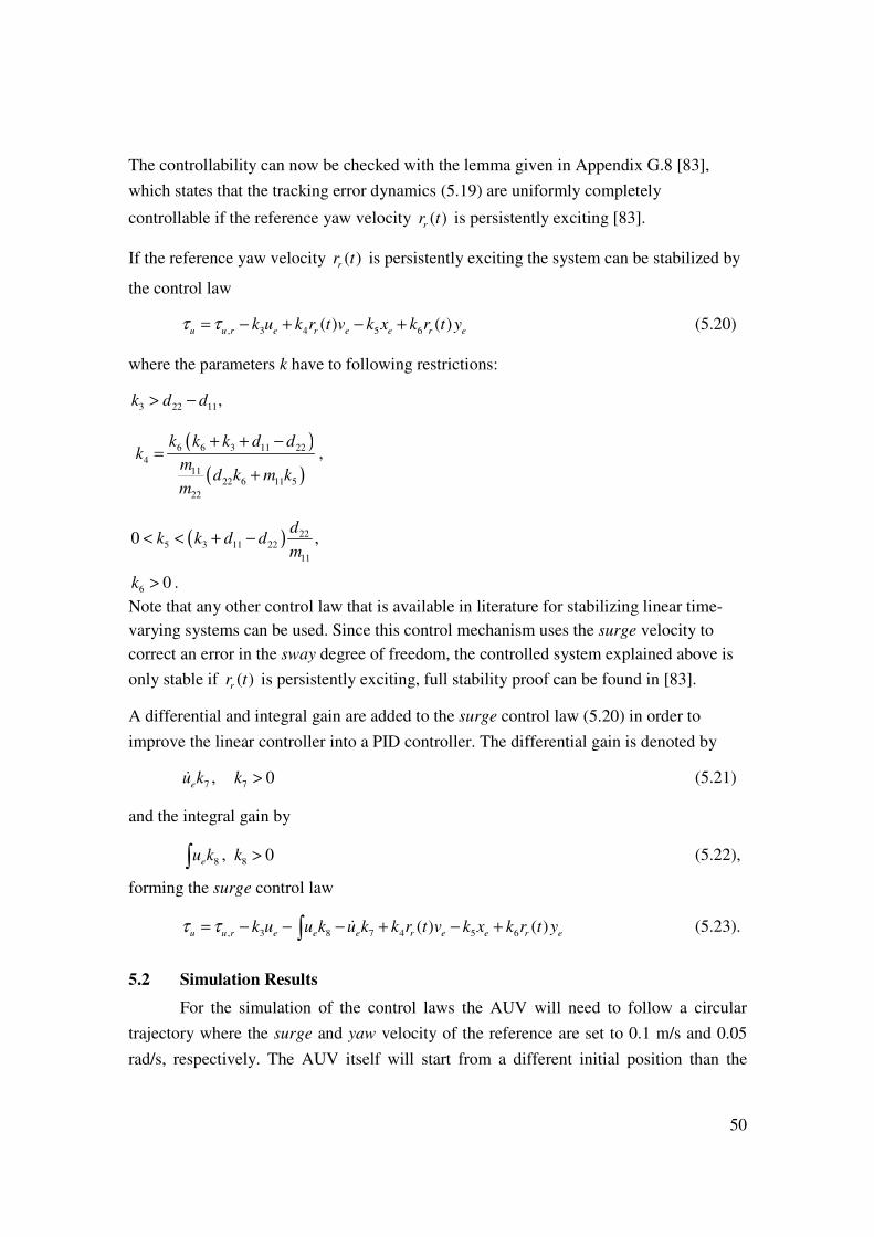
50

The controllability can now be checked with the lemma given in Appendix G.8 [83],

which states that the tracking error dynamics (5.19) are uniformly completely

controllable if the reference yaw velocity ( )rr t is persistently exciting [83].

If the reference yaw velocity ( )rr t is persistently exciting the system can be stabilized by

the control law

, 3 4 5 6( ) ( )u u r e r e e r ek u k r t v k x k r t yτ τ= − + − + (5.20)

where the parameters k have to following restrictions:

3 22 11,k d d> −

( )

( )

6 6 3 11 22

411

22 6 11 5

22

k k k d dk

md k m k

m

+ + −=

+

,

( ) 225 3 11 22

11

0 , d

k k d dm

< < + −

6 0k > .

Note that any other control law that is available in literature for stabilizing linear time-

varying systems can be used. Since this control mechanism uses the surge velocity to

correct an error in the sway degree of freedom, the controlled system explained above is

only stable if ( )rr t is persistently exciting, full stability proof can be found in [83].

A differential and integral gain are added to the surge control law (5.20) in order to

improve the linear controller into a PID controller. The differential gain is denoted by

7eu k& , 7 0k > (5.21)

and the integral gain by

8eu k∫ , 8 0k > (5.22),

forming the surge control law

, 3 8 7 4 5 6( ) ( )u u r e e e r e e r ek u u k u k k r t v k x k r t yτ τ= − − − + − +∫ & (5.23).

5.2 Simulation Results

For the simulation of the control laws the AUV will need to follow a circular

trajectory where the surge and yaw velocity of the reference are set to 0.1 m/s and 0.05

rad/s, respectively. The AUV itself will start from a different initial position than the

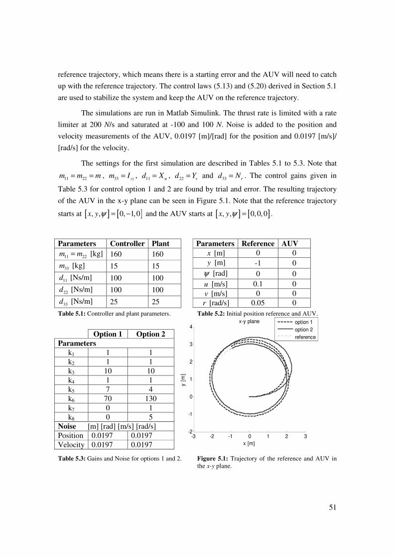
51

reference trajectory, which means there is a starting error and the AUV will need to catch

up with the reference trajectory. The control laws (5.13) and (5.20) derived in Section 5.1

are used to stabilize the system and keep the AUV on the reference trajectory.

The simulations are run in Matlab Simulink. The thrust rate is limited with a rate

limiter at 200 N/s and saturated at -100 and 100 N. Noise is added to the position and

velocity measurements of the AUV, 0.0197 [m]/[rad] for the position and 0.0197 [m/s]/

[rad/s] for the velocity.

The settings for the first simulation are described in Tables 5.1 to 5.3. Note that

11 22m m m= = , 33 zzm I= , 11 ud X= , 22 vd Y= and 33 rd N= . The control gains given in

Table 5.3 for control option 1 and 2 are found by trial and error. The resulting trajectory

of the AUV in the x-y plane can be seen in Figure 5.1. Note that the reference trajectory

starts at [ ] [ ], , 0, 1,0x y ψ = − and the AUV starts at [ ] [ ], , 0,0,0x y ψ = .

Table 5.1: Controller and plant parameters. Table 5.2: Initial position reference and AUV.

-3 -2 -1 0 1 2 3-2

-1

0

1

2

3

4

x [m]

y [

m]

x-y plane

option 1

option 2

reference

Table 5.3: Gains and Noise for options 1 and 2. Figure 5.1: Trajectory of the reference and AUV in

the x-y plane.


11 22m m= [kg] 160 160

33m [kg] 15 15

11d [Ns/m] 100 100

22d [Ns/m] 100 100

33d [Ns/m] 25 25

Parameters Reference AUV

x [m] 0 0

y [m] -1 0

ψ [rad] 0 0

u [m/s] 0.1 0

v [m/s] 0 0

r [rad/s] 0.05 0

Option 1 Option 2

Parameters

k1 1 1

k2 1 1

k3 10 10

k4 1 1

k5 7 4

k6 70 130

k7 0 1

k8 0 5

Noise [m] [rad] [m/s] [rad/s]

Position 0.0197 0.0197

Velocity 0.0197 0.0197

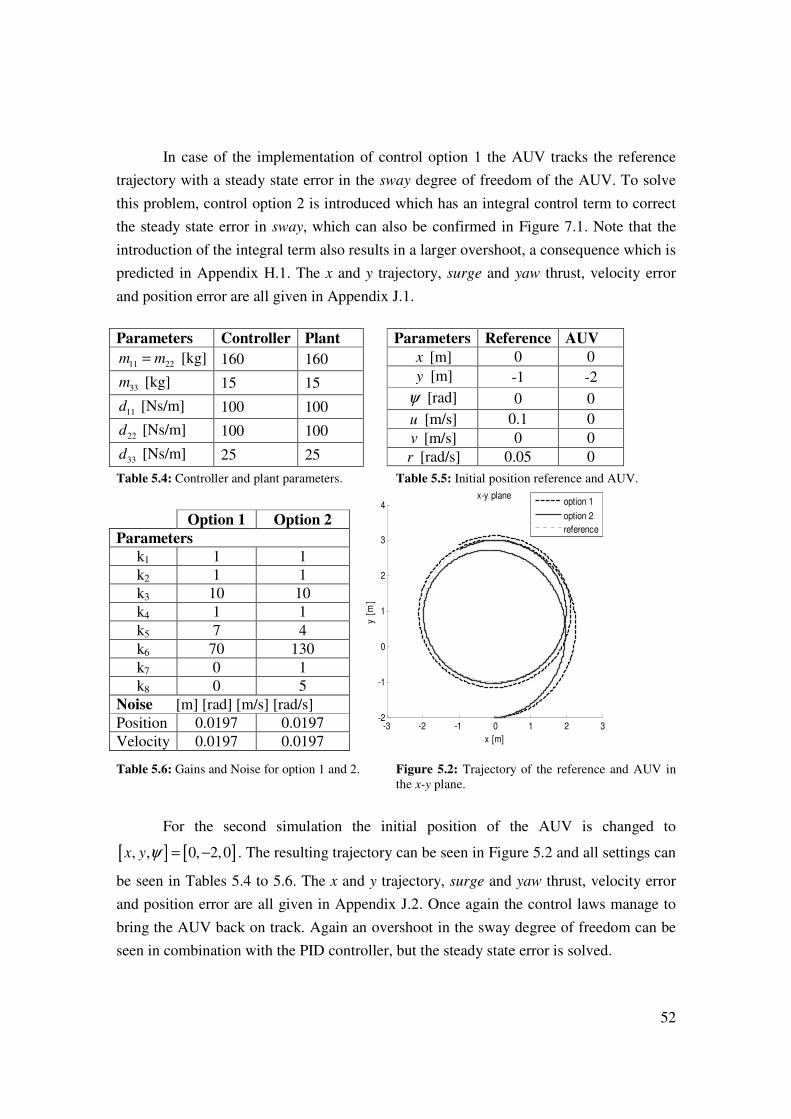
52

In case of the implementation of control option 1 the AUV tracks the reference

trajectory with a steady state error in the sway degree of freedom of the AUV. To solve

this problem, control option 2 is introduced which has an integral control term to correct

the steady state error in sway, which can also be confirmed in Figure 7.1. Note that the

introduction of the integral term also results in a larger overshoot, a consequence which is

predicted in Appendix H.1. The x and y trajectory, surge and yaw thrust, velocity error

and position error are all given in Appendix J.1.

Table 5.4: Controller and plant parameters. Table 5.5: Initial position reference and AUV.

-3 -2 -1 0 1 2 3-2

-1

0

1

2

3

4

x [m]

y [

m]

x-y plane

option 1

option 2

reference

Table 5.6: Gains and Noise for option 1 and 2. Figure 5.2: Trajectory of the reference and AUV in

the x-y plane.

For the second simulation the initial position of the AUV is changed to

[ ] [ ], , 0, 2,0x y ψ = − . The resulting trajectory can be seen in Figure 5.2 and all settings can

be seen in Tables 5.4 to 5.6. The x and y trajectory, surge and yaw thrust, velocity error

and position error are all given in Appendix J.2. Once again the control laws manage to

bring the AUV back on track. Again an overshoot in the sway degree of freedom can be

seen in combination with the PID controller, but the steady state error is solved.


11 22m m= [kg] 160 160

33m [kg] 15 15

11d [Ns/m] 100 100

22d [Ns/m] 100 100

33d [Ns/m] 25 25

Parameters Reference AUV

x [m] 0 0

y [m] -1 -2

ψ [rad] 0 0

u [m/s] 0.1 0

v [m/s] 0 0

r [rad/s] 0.05 0

Option 1 Option 2

Parameters

k1 1 1

k2 1 1

k3 10 10

k4 1 1

k5 7 4

k6 70 130

k7 0 1

k8 0 5

Noise [m] [rad] [m/s] [rad/s]

Position 0.0197 0.0197

Velocity 0.0197 0.0197

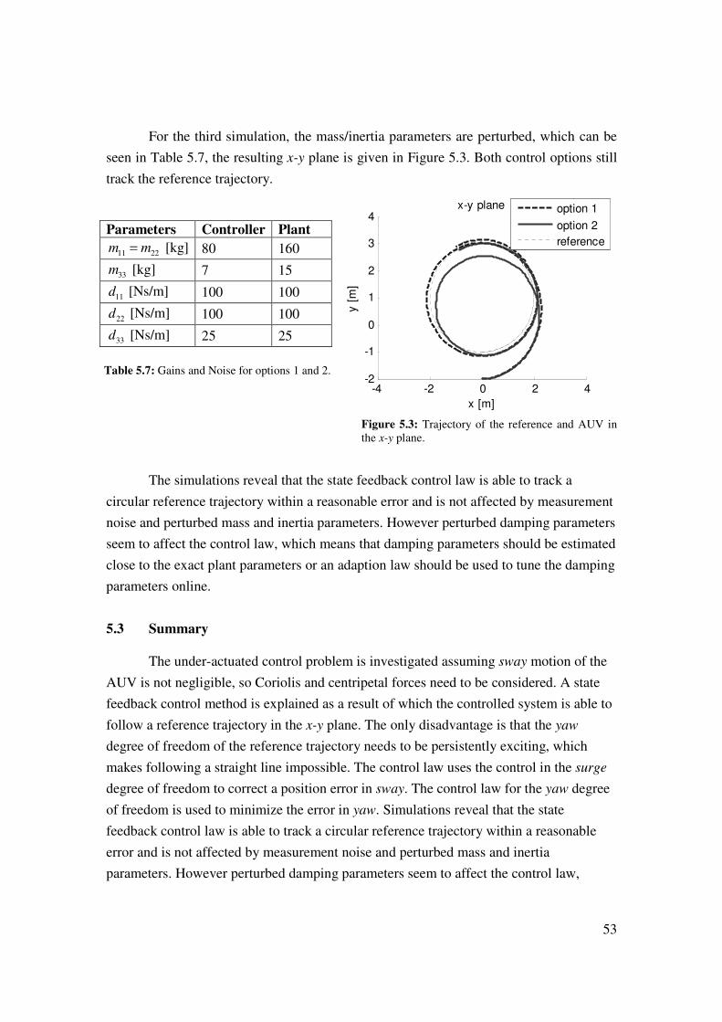
53

For the third simulation, the mass/inertia parameters are perturbed, which can be

seen in Table 5.7, the resulting x-y plane is given in Figure 5.3. Both control options still

track the reference trajectory.

-4 -2 0 2 4-2

-1

0

1

2

3

4

x [m]

y [

m]

x-y plane

option 1

option 2

reference

Figure 5.3: Trajectory of the reference and AUV in

the x-y plane.

The simulations reveal that the state feedback control law is able to track a

circular reference trajectory within a reasonable error and is not affected by measurement

noise and perturbed mass and inertia parameters. However perturbed damping parameters

seem to affect the control law, which means that damping parameters should be estimated

close to the exact plant parameters or an adaption law should be used to tune the damping

parameters online.

5.3 Summary

The under-actuated control problem is investigated assuming sway motion of the

AUV is not negligible, so Coriolis and centripetal forces need to be considered. A state

feedback control method is explained as a result of which the controlled system is able to

follow a reference trajectory in the x-y plane. The only disadvantage is that the yaw

degree of freedom of the reference trajectory needs to be persistently exciting, which

makes following a straight line impossible. The control law uses the control in the surge

degree of freedom to correct a position error in sway. The control law for the yaw degree

of freedom is used to minimize the error in yaw. Simulations reveal that the state

feedback control law is able to track a circular reference trajectory within a reasonable

error and is not affected by measurement noise and perturbed mass and inertia

parameters. However perturbed damping parameters seem to affect the control law,


11 22m m= [kg] 80 160

33m [kg] 7 15

11d [Ns/m] 100 100

22d [Ns/m] 100 100

33d [Ns/m] 25 25

Table 5.7: Gains and Noise for options 1 and 2.

54

which means that damping parameters should be estimated close to the exact plant

parameters or an adaption law should be used to tune the damping parameters online.

55

Chapter 6

Conclusions and Recommendations

6.1 Conclusions

The kinematic and dynamic models of the AUV of the Department of Mechanical

Engineering at the University of Canterbury are derived for its six degrees of freedom

operating range. The following assumptions are made to the dynamic model: the AUV

only moves with a relatively low speed, there is symmetry about the three planes, the

aligning moment ensures horizontal stability, roll, pitch and sway motion can be

neglected, and, the body-fixed frame of the AUV is positioned at the center of gravity.

With these assumptions decoupling the degrees of freedom is possible, where only the

surge, heave and yaw degrees of freedom will be controlled. Since one is dealing with a

decoupled model only the mass/inertia and damping terms need to be estimated. A

system identification approach is proposed which treats the surge, heave and yaw degree

of freedom separately. The approach uses a static experiment to determine the damping

terms, where the acceleration is zero, and, a dynamic experiment to determine the mass

terms, with the use of constant acceleration. Unfortunately due to the failure of the IMU

the acceleration could not be measured correctly. Therefore the unknown mass/inertia

and damping terms could not be estimated and a parameter selection method is used

instead. The parameter selection is based on parameter estimation results of software

programs and a parameter comparison with other similarly shaped AUVs.

After comparing different control techniques a feedback linearizing control

technique is chosen to design control laws for the surge, heave and yaw degrees of

freedom. The feedback linearizing control technique changes the nonlinear dynamical

56

system into a linear system through a suitable chosen control input. The linear system is

stabilized with the use of PID control. The feedback linearizing controller is extended to a

tracking controller in order to track a trajectory in one degree of freedom. Simulations are

performed to test the controller, which performed well under parameter perturbation and

the implementation of noise on the feedback position and velocity signals of the plant. It

should be noted that all states need to be available online to control the AUV. However

during experiments full state measurement is not possible and the control law should be

extended with an observer in order to estimate unmeasured states.

In the x-y plane the AUV is only able to move in the surge and yaw degrees of

freedom caused by the trolling motor configuration. An under-actuated control problem

arises, since one is only able to control two degrees of freedom while the AUV is able to

move in three degrees of freedom. To steer the AUV with a smooth motion from an

initial position A to a different position B, in the x-y plane, a path planning model is

derived. The path planning model describes a path from A to B with the use of polar

coordinates which the AUV is able to follow controlling only the surge and yaw degrees

of freedom. The assumption is made that sway-motion of the AUV can be neglected.

From simulations with the path planning model it could be concluded that the path

planning model works correct, except for planning a straight line due to singularity

reasons. This problem can be solved by introducing a switching controller which is able

to switch between different path planning models.

The under-actuated control problem is again investigated, now assuming sway

motion of the AUV is not negligible, so Coriolis and centripetal forces need to be

considered. A state feedback control method is explained as a result of which the

controlled system is able to follow a reference trajectory in the x-y plane. The only

disadvantage is that the yaw degree of freedom of the reference trajectory needs to be

persistently exciting, which makes following a straight line impossible. The control law

uses the control in the surge degree of freedom to correct a position error in sway. The

control law for the yaw degree of freedom is used to minimize the error in yaw.

Simulations reveal that the state feedback control law is able to track a circular reference

trajectory within a reasonable error and is not affected by measurement noise and

perturbed mass and inertia parameters. However perturbed damping parameters seem to

affect the control law, which means that damping parameters should be estimated close to

the exact plant parameters or an adaption law should be used to tune the damping

parameters online.

57

6.2 Recommendations

A few recommendations can be made about the AUV design, sensor equipment

and future experiments. At first, the trolling motor configuration should be redesigned to

improve the water flow, thrust power and weight of the vehicle. The frame which holds

the trolling motors and battery compartments can be designed more compact, reducing

the weight of the vehicle, and, the vertical trolling motors should be repositioned in order

to improve the flow of the horizontal trolling motors.

New sensor equipment should be installed to determine the position and velocity

of the AUV. Different sensors are available, but the best low-cost solution will be stereo

vision. Two underwater cameras measure the displacement of the AUV with respect to

objects placed on the bottom of a swimming pool determining the relative position and

velocity of the AUV. If position and velocity measurements of the AUV are possible, the

unknown parameters can be estimated with the use of the system identification approach

explained in this report. The data acquisition is a very time consuming and challenging

task and demands a proper setup and planning for correct measurements. Parameters

should be estimated with the highest possible accuracy which finally will lead to better

and more accurate control laws.

If the unknown parameters are estimated, control techniques explained in this

report extended with state observers can be used for positioning the AUV. Although, for

the under-actuated problem a global tracking controller still needs to be designed.

59

Bibliography

[1] D. Richard Blidberg. The Development of Autonomous Underwater Vehicles (AUV); A Brief

Summary. Autonomous Undersea Systems Institute, 2000.

[2] P.J. Craven, R. Sutton and R.S. Burns. Control Strategies for Unmanned Underwater Vehicles.

University of Plymouth, 1998; Key Information: PID control, Gain-scheduling control, adaptive control, MRAC,

indirect adaptive control, self-tuning control, sliding control, H-infinity robust control, fuzzy logic control

[3] Ferial El-Hawary. The Ocean Engineering Handbook, The Electrical Engineering Handbook

Series, 2001

[4] R. Cristi, F.A. Papoulias and A.J. Healey. Adaptive Sliding Mode Control of Autonomous

Underwater Vehicles in the Dive Plane. IEEE journal of oceanic engineering, vol. 15, no. 3, pag.

152-160, july 1990

[5] R. Burgoyne, X. Huang, C. North, N. Schaal and K. Shaw. Final Year Project Report; Unmanned

Underwater Vehicle. University of Canterbury; 2007; Key Information: Design of the AUV of the University

of Canterbury

[6] G.N. Roberts and R. Sutton. Advances in unmanned marine vehicles. Book IEE control series 69,

2006

[7] K.P. Valanis, D. Gracanin, M. Matijasevic, R.Kolluru and A. Demetriou. Control architecture for

autonomous underwater vehicles. IEEE Control Systems, issue no. 0272-1708l97l, pag. 48-60

Dec.1997

[8] Thor I. Fossen. Underwater Vehicle Dynamics. Book TSI Press, Albuquerque, 1995.

[9] W. Wang and C. M. Clark. Modeling and Simulation of the VideoRay Pro III Underwater Vehicle.

University of Waterloo, 2001; Key Information: Kinematic Model, Dynamic model

[10] B. Jalving. The NDRE-AUV flight control system. IEEE journal of Oceanic Engineering vol. 19,

no. 4, pag. 497-501, oct.1994; Key Information: PID control, autopilots, vehicle modeling

[11] O. Fjellstad and T.I. Fossen. Position and attitude tracking of AUVs: a quaternion feedback

approach. Department of Engineering Cybernetics, The Norwegian Institute of Technology,

University of Trondheim, Nov 1994.

[12] G. Antonelli, S. Chiaverini, N. Sarkar, and M. West. Adaptive control of a autonomous

underwater vehicle: experimental results on ODIN. IEEE Transactions on Control Systems

Technology, vol. 9, no. 5, pag.756-765, sep. 2001; Key Information: Adaptive Control, position control, AUV:

ODIN

[13] J. Healey and D. Lienard. Multivariable sliding model control for autonomous diving and steering

of unmanned underwater vehicles. IEEE Journal of Oceanic Engineering, vol. 18, no. 3, pag. 327-

339, 1993; Key Information: Sliding Mode Control, Vehicle Modeling, Flight UUV

60

[14] D.B. Marco, A.J. Healey. Command, control and navigation experimental results with the NPS

ARIES AUV. IEEE Journal of Oceanic Engineering, vol. 26, no. 4, pag. 466-476, 2001; Key

Information: Kalman filter, Autopilot Control Laws, AUV: ARIES

[15] J. Hu, C. Bohn, and H.R. Wu. Systematic H∞ weighting function selection and its application to

the real-time control of a vertical take-off aircraft. Control Engineering Practice 8, pag. 241-252

2000; Key Information: H∞ weighting function

[16] C. Silpa-Anan. Autonomous underwater vehicle: Vision and control. Master’s thesis, The

Australian National University, 2001; Key Information: AUV Thesis, AUV: Kambara

[17] G. Indiveri. Modelling and Identification of Underwater Robotics Systems. PhD thesis, University

of Genova, 1998; Key Information: AUV Thesis, AUV: ROMEO

[18] P. Brutzman. A Virtual World for an Autonomous Underwater Vehicle. PhD thesis, Naval

Postgraduate School, 1994.

[19] D. Wettergreen et al. Development of autonomous underwater vehicle towards visual servo

control. Proceedings of the Australian Conference on Robotics and Automation 2000, 2000.

[20] T. Fossen and I. Fjellstad. Robust adaptive control of underwater vehicles. 3rd

IFAC Workshop on Control Applications in Marine Systems (CAMS ‘95), pag. 1-9, 1995; Key

Information: Adaptive control

[21] S. Sagatun and R. Johansson. Optimal and adaptive control of underwater vehicles. 4th

Symposium on Robot Control, pag. 953-958, 1994; Key Information: Adaptive control

[22] J.Nie, T. Fossen et al. On-board sensor-based adaptive control of small uuvs in very shallow

water. Proceedings of the IFAC Conference on Control Applications in Marine Systems (CAMS

’98), pag. 441-452, 1998; Key Information: Adaptive control

[23] T. Fossen and S. Sagatun. Adaptive control of nonlinear underwater robotic systems. Journal of

Robotic Systems, JRS-8(3): pag. 393-412, 1991; Key Information: Adaptive control

[24] Pascoal, Oliveira, Santos, and others. Robotic Ocean Vehicles for Marine Science Applications:

the European ASIMOV Project; IEEE no. 0-7803-6551-8, 2000. Key Information: Infante AUV,

communication and sonar, sensors

[25] T. Fossen and B. Foss. Sliding control of mimo nonlinear systems. Proceedings of the European

Control Conference, pag. 1855-1860, 1991; Key Information: Sliding mode control

[26] J. Healey and D. Lienard. Adaptive sliding mode control of autonomous underwater vehicles in

the dive plane. IEEE Journal of Oceanic Engineering, vol. 15, no. 3, pag. 152-161, july 1990; Key

Information: Sliding mode control

[27] S. Feijun and S. Smith. Automatic design and optimization of fuzzy logic controllers for an

autonomous underwater vehicle. OCEANS’2000 MTS/IEEE, no. 0-7803-6551-8, pag. 829-835,

2000;Key Information: Fuzzy Logic Control

[28] M. Kwiesielewicz et al. Predictive versus fuzzy control of autonomous underwater vehicle. IEEE

International Conference on Methods and Models in Automation and Robotics, 2001.

[29] S. Feijun and S. Smith. Design of sliding mode fuzzy controllers for an autonomous underwater

vehicle without system model. OCEANS’2000 MTS/IEEE, vol.2, pag 835-840, 2000.

[30] J.Jantzen. Design Of Fuzzy Controllers. Technical University of Denmark. 1998; Key Information:

Basic Explanation Fuzzy Control

[31] B.Ashbaugh and J.Boitano. Advantages and Disadvantages of Controller Designs Using Fuzzy

Logic. University of California, 1998. Key Information: Fuzzy Logic Control

[32] J. Ibaiiez-Guzmhl and R. Ketata. Fuzzy logic control experiments on a singlelink manipulator.

PBle Atlantique de Genie Electrique; Key Information: Fuzzy Logic Control

61

[33] S.M. Smith, G.J.S. Rae, and D.T. Anderson. Applications of Fuzzy Logic to the Control of an

Autonomous Underwater Vehicle. Advanced Marine Systems Group Department of Ocean

Engineering, pag 1099-1106, 1992; Key Information: Fuzzy Logic Control (heading, pitch and depth), AUV:

Ocean Voyager

[34] W. Naeem et al. Lqg/ltr control of an autonomous underwater vehicle using a hybrid guidance

law. International Federation on Automatic Control Journal, 2003; Key Information: Linear Quadratic

Gaussian methods, Kalman Filter

[35] D. Juul et al. Submersible control using the linear quadratic gaussian with loop transfer recovery

method. Proceedings of the Symposium on Autonomous Underwater Technology, 1994.

[36] A. Santos, R.R. Bitmead. Nonlinear Control for an Autonomous Underwater Vehicle (AUV)

Preserving Linear Design Capabilities. Conference on Decision & Control. 1995 Key Information: Linear Quadratic Gaussian methods, Extended Kalman Filter

[37] T.I. Fossen. Guidance and Control of Ocean Vehicles. Book: John Wiley and Sons Ltd. 1994

[38] T.I. Fossen. Marine Control Systems. Guidance, Navigation and Control of Ships, Rigs and

Underwater Vehicles. Marine Cybernetics AS. 2002

[39] J.Lee, M.Roh, J.Lee and D.Lee. Clonal Selection Algorithms for 6-DOF PID Control of

Autonoumous Underwater Vehicles. Department of Bio and Brian Engineering, KAIST; Key

Information: PID control

[40] K.P. Valavanis, D. Gracanin, M. Matijasevic and others. Control Architectures for Autonomous

Underwater Vehicles, IEEE Control Systems, no. 0272-1708, pag. 48-64, 1997; Key Information:

Comparison of different control techniques in different AUVs

[41] R.Bachmayer, S.Humphris, D. Fornari, and others. Oceanographic Research Using Remotely

Operated Underwater Robotic Vehicles: Exploration of Hydrothermal Vent Sites On The Mid-

Atlantic Ridge At 37°North 32°West. 1996; Key Information: Basic Information AUV, Navigation, Sonar, AUV:

ARGO2

[42] S.B. Williams, P.Newman, G.Dissanayake and others. A decoupled, distributed AUV control

architecture. University of Sydney, 2006; Key Information: Decoupled control, AUV: Oberon

[43] P. Mhaskar, N.H. El-Farra and P.D.Christofides. A Method for PID Controller Tuning Using

Nonlinear Control Techniques. University of California, 2004; Key Information: PID control, tuning

methods and nonlinear control

[44] K.Hur. Brushless Motor Controller for an AUV. University of Texas, 2006; Key Information: Basic

AUV Information

[45] L.A.Gonzales. Design, Modeling and Control of an Autonomous Underwater Vehicle. Mobile

Robotics Laboratory, University of Western Australia, 2004; Key Information: AUV Thesis, AUV: MAKO

[46] M.H.Kim, Nonlinear Control and Robust Observer Design for Marine Vehicles. Virginia

Polytechnic Institute and State University, 2000; Key Information: Nonlinear control, Nonlinear observer,

neural networks, sliding and adaptive

[47] D.G.Biddle. Inertial Based Control on the Kambara. Australian National University, 2003; Key

Information: IMU control, AUV thesis, AUV: Kambara

[48] O.E.Fjellstad. Control of Unmanned Underwater Vehicles in Six Degrees of Freedom, A

Quaternion Feedback Approach. University of Trondheim. 1994; Key Information: AUV Thesis, AUV:

MOBATEL

[49] I. Schjolber and T.I. Fossen. Modelling and Control of Underwater Vehicle Manipulator Systems.

University of Trondheim; Key Information: Dynamic model, feedback linearization

[50] D.A. Jones, D.B. Clarke, I.B. Brayshaw and others. The Calculation of Hydrodynamic

Coefficients for Underwater Vehicles. Australia; Key Information: Dynamic model, Parameter Estimation,

Identification

[51] P.Ridao, J.Batlle and M.Carreras. Model Identification of a low-speed UUV. University of Girona,

2001; Key Information: Parameter Estimation, Modeling, Identification

62

[52] J. Wu, M.J. Zhang, Y.J. Wang. Research of system identification method for underwater vehicle

based on neural network. Harbin Engineering University, 2007; Key Information: Parameter estimation,

system identification

[53] P.Hsu, M. Bodson, S.Sastry and B.Paden. Adaptive Identification and Control for Manipulators

without Using Joint Accelerations. University of California; Key Information: Dynamic model, Parameter

estimation, Adaptive Control, Identification

[54] A. Tiano. Comparison of nonlinear identification methods for underwater vehicles. University of

Pavia; Key Information: Lyapunov Identification, Least Squares Identification, Parameter estimation, Modeling,

Identification

[55] D.A. Smallwoord. Adaptive Identification of Dynamically Positioned Underwater Robotic

Vehicles; Key Information: Adaptive Parameter Estimation, Dynamic model, Least Squares Method, Identification

[56] P.Ridao, A.Tiano, A. El-Fakdi, M.Carreras, A.Zirilli. On the identification of nonlinear models of

unmanned underwater vehicles. University of Girona, 2004; Key Information: Dynamic model, Parameter

Estimation, Identification

[57] A.Alessandri, M.Caccia, G.Indiveri, F.Veruggio. Application of LS and EKF Techniques to the

identification of underwater vehicles. University of Genoa, 1998; Key Information: Dynamic model,

Identification, Least Square, Extended Kalman Filter

[58] A. Tiano, R.Sutton, A.Lozowicki, W.Naeem. Observer Kalman filter identification of an

autonomous underwater vehicle, 2006; Key Information: System identification, Parameter Estimation, Dynamic

model

[59] J.S. Geisbert. Hydrodynamic Modeling for Autonomous Underwater Vehicles Using Computional

and Semi-Empirical Methods. Verginia Polytechnis Institute and State University, 2007; Key

Information: Kinematic model, Dynamic model

[60] A.J. Healey, S.M. Rock and others. Toward an Improved Understanding of Thruster Dynamics for

Underwater Vehicles. IEEE journal of oceanic engineering, vol 20, no. 4, pag. 354-361, okt. 1995; Key Information: Thruster model

[61] T.I.Fossen and O.E.Fjellstad. Robust Adaptive Control of Underwater Vehicles: A comparative

study. University of Trondheim, IFAC workshop on Control Applications in Marine Systems

(CAMS’95), 1995; Key Information: Adaptive control, dynamic model, parameter estimation

[62] D.B.Marco, A.Martins, A.J.Healey. Surge Motion Parameter Identification for the NPS Phoenix

AUV, 1996; Key Information: Parameter Estimation, Kalman filter

[63] L.L. Whitcomb, D.R. Yoerger. Comparative Experiments in the Dynamic and Model-Based

Control of Marine Thrusters, pag. 1018-1028, 1994; Key Information: Thruster model

[64] C.L. Tsukamoto, W.Lee, J.Yuh, S.K.Choi and J.Lorentz. Comparison study on advanced thruster

control of underwater robots. University of Hawaii, 1997; Key Information: Thruster model

[65] J. Petrich, W.L.Neu and D.J.Stilwell. Identification of a simplied AUV pitch axis model for

control design: Theory and experiments. Virginia Polytechnic Institute and State University, 2001; Key Information: System Identification, modeling

[66] M.Caccia, G.Indiveri and Gianmarco Veruggio. Modeling and Identification of Open-Frame

Variable Configuration Unmanned Underwater Vehicles, IEEE journal of oceanis engineering,

vol. 25, no. 2, pag. 227-241, apr. 2000; Key Information: Parameter estimation, thruster model, decoupling

[67] K.R.Goheen and E.R.Jefferys. Multivariable self-tuning autopilots for autonomous and remotely

operated underwater vehicles. IEEE journal Oceanic Engineering, vol 15, no. 3, pag. 144-151,

1990; Key Information: Thruster model, implementation of the thruster installation coefficient.

[68] C.Moler. Numerical Computing with Matlab, Least Squares, Chpt 5. Mathworks, 2008; Key

Information: Least Squares Technique

[69] D. Mills and C. Harris. Neurofuzzy modelling and control of a six degree of freedom auv. 1996.

63

[70] V. Filaretov et al. The sliding mode adaptive control system for autonomous underwater robot.

Proceedings of ICAR ’95, 1995.

[71] D. Sellers. An Overview of Proportional plus Integral plus Derivative Control and Suggestions for

Its Successful Application and Implementation. Portland Energy Conservation Inc, 2003.

[72] P. Mhaskar, N. H. El-Farra and P. D. Christofides. A Method for PID Controller Tuning Using

Nonlinear Control Techniques. Proceeding of the 2004 American Control Conference, no. 7803-

8335-4, pag. 2925-3000, Jun 2004

[73] J.E.Slottine and W.Li. Applied nonlinear control. Book: Prentice-Hall, 1991; Key Information:

Nonlinear control techniques

[74] H.K.Khalil. Nonlinear systems. Third edition. Book: Prentice-Hall, 2002; Key Information: Nonlinear

control techniques

[75] G.F.Franklin, J.D.Powell and A.Emami-Naeini. Feedback control of dynamic systems. Fourth

Edition. Book: Prentice-Hall, 2002; Key Information: Feedback control

[76] M.W.Spong, S.Hutchinson and M.Vidyasagar. Robot modeling and control. Book: Wiley, 2006; Key Information: Path tracking

[77] P.Egeskov, A.Bjerrum, et.al.. Design, construction and hydrodynamic testing of the AUV

MARIUS. Proceedings of the AUV conference, 1994; Key Information: Gain scheduling

[78] M.Aicardi, G.Casalino, et.al. Closed loop steering of unicycle-like vehicles via Lyapunov

Techniques. IEEE Robotics & Automation Magazine, pag. 27-35, mar.1995; Key Information: Unicycle

Path Planning

[79] M.Aicardi, G.Casalino, et.al. Closed loop smooth steering of unicycle-like vehicles. IEEE

proceedings of the 33rd Conference on Decision and Contol, no. 0-7803-1986-0, pag. 2455-2459,

Dec 1994; Key Information: Unicycle Path Planning

[80] T.S.VanZwieten. Dynamic simulation and control of an autonomous surface vehicle. Florida

Atlantic University, 2003; Key Information: Unicycle Path Planning applied on a ASV

[81] A.Micaelli and C.Samson. Trajectory tracking for unicycle-type and two-steering-wheels mobile

robots. Unite´ de recherche INRIA Sophia-Antipolis, 1993; Key Information: Unicycle Path Planning and

tracking

[82] A.P.Aguiar and J.P.Hespanha. Trajectory-Tracking and Path-Following of Underactuated

Autonomous Vehicles With Parametric Modeling Uncertainty. IEEE Transactions on automatic

control, vol 52, no. 8, pag. 1362-1379, aug 2007; Key Information: Trajectory Tracking and Path Following of

an AUV

[83] A.A.J.Lefeber. Tracking control of nonlinear mechanical systems. Universiteit Twente, 2000; Key

Information: Tracking control of a ship and unicycle

[84] K.D.Do and J.Pan. Robust and adaptive path following for underactuated autonomous underwater

vehicles. The University of Western Australia, 2003; Key Information: Path following of an AUV using

backstepping

[85] L.Lapierre and D.Soetanto. Nonlinear path-following control of an AUV. Ocean engineering, vol

34, pag. 1734-1744, 2007; Key Information: Path following of an AUV using backstepping

[86] L.Lapierre, D.Soetanto and A.Pascoal. Nonlinear Path Following with Applications to the Control

of Autonomous Underwater Vehicles. Proceedings of the 42nd

IEEE Conference on Decision and

Control, no. 0-7803-7924-1, pag. 1256-1261, 2003; Key Information: Path following of an AUV using

backstepping and applications

[87] P.Encarnasiio and A.Pascoal. 3D Path Following for Autonomous Underwater Vehicle.

Proceedings of the 39th

IEEE Conference on Decision and Control, no. 0-7803-6638-7, pag. 2977-

2983, Dec 2000; Key Information: 3D path following using backstepping

64

[88] E.Lefeber, K.Y.Pettersen and H.Nijmeijer. Tracking Control of an Underactuated Ship. IEEE

Transactions on control systems technology, vol 11, no. 1, pag. 52-61, jan 2003; Key Information:

Tracking control of a ship using cascaded controller design see also [83]

[89] K.Y.Pettersen and H.Nijmeijer. Tracking control of an underactuated surface vessel. Norwegian

University of Science and Technology, University of Twente, Technical Univeristy of Eindhoven,

1998; Key Information: Tracking control of a ship

[90] K.D.Do, Z.P.Jiang, J.Pan and H.Nijmeijer. Global output feedback universal controller for

stabilization and tracking of underactuaded ODIN-an underwater vehicle. University of Western

Australia, Polytechnic University NY USA, Eindhoven University of Technology. Proceedings of

the 41st IEEE Conference on Decision and Control, no. 0-7803-7516-5, pag. 504-510, Dec 2002;

Key Information: Tracking control for the AUV named ODIN, see also [91]

[91] K.D.Do, Z.P.Jiang, J.Pan and H.Nijmeijer. A global output-feedback controller for

stabilization and tracking of underactuated ODIN: A spherical underwater vehicle. University of Western Australia, Polytechnic University NY USA, Eindhoven University of

Technology. Automatica 40, 2004; Key Information: Tracking control for the AUV named ODIN, see also [90]

[92] K.Y.Pettersen and O.Egeland. Exponential stabilization of an underactuated surface vessel.

Proceedings of the 35th

IEEE Conference on Decision and Control, no. 0-7803-3590-2, pag. 967-

973, Dec 1996; Key Information: Underactuaded control

[93] K.Y.Pettersen and O.Egeland. Time-varying Exponential Stabilization of the Position and Attitude

of an Underactuated Autonomous Underwater Vehicle. Norwegian University of Science and

Technology, 1997; Key Information: Underactuaded control

[94] T.Patterson, H.Rogers, D.Hewett, F.McKenzie and B.Burnell, Final Year Project Report;

Unmanned Underwater Vehicle. University of Canterbury; 2008; Key Information: Design of the AUV of

the University of Canterbury

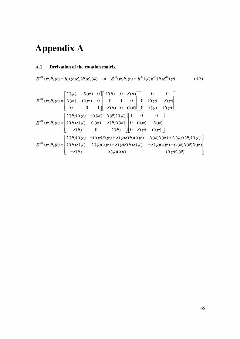
65

Appendix A

A.1 Derivation of the rotation matrix

30 32 21 10( , , ) ( ) ( ) ( ) or ( , , ) ( ) ( ) ( ) (3.3)

( ) ( ) 0 ( ) 0 ( ) 1 0 0

( , , ) ( ) ( ) 0 0 1 0 0 ( ) ( )

0 0 1 ( ) 0 ( ) 0 ( ) ( )

( ,

BW

z y x

BW

BW

R R R R R R R R

C S C S

R S C C S

S C S C

R

ϕ θ ψ ψ θ ϕ ϕ θ ψ ψ θ ϕ

ψ ψ θ θ

ϕ θ ψ ψ ψ ϕ ϕ

θ θ ϕ ϕ

ϕ θ

= =

− = − −

( ) ( ) ( ) ( ) ( ) 1 0 0

, ) ( ) ( ) ( ) ( ) ( ) 0 ( ) ( )

( ) 0 ( ) 0 ( ) ( )

( ) ( ) ( ) ( ) ( ) ( ) ( ) ( ) ( ) ( ) ( ) ( )

( , , ) ( ) ( ) ( ) ( ) ( ) ( ) ( ) ( ) ( ) (BW

C C S S C

C S C S S C S

S C S C

C C C S S S C S S C S C

R C S C C S S S S C C

θ ψ ψ θ ψ

ψ θ ψ ψ θ ψ ϕ ϕ

θ θ ϕ ϕ

θ ψ ϕ ψ ϕ θ ψ ϕ ψ ϕ θ ψ

ϕ θ ψ θ ψ ϕ ψ ϕ θ ψ ϕ ψ

− = − −

− + +

= + − + ) ( ) ( )

( ) ( ) ( ) ( ) ( )

S S

S S C C C

ϕ θ ψ

θ ϕ θ ϕ θ

−

66

A.2 Derivation of the coordinate transform matrix

1

2 which gives:

0 0

0 ( ) ( ) ( ) 0

0 0

Substitution of the rotation matrices :

1 0 0

0 0 ( ) ( )

0 0 ( ) ( )

T T T

T T

B W

B B B

B x x y

B B

B

J

e e R e R R

e e C S

S C

ω ω

ϕ

ω ϕ θ ϕ θ

ψ

ϕ

ω ϕ ϕ

ϕ ϕ

−=

= + +

= + −

r r

&r r r r&

&

&r r r

0 1 0 0 ( ) 0 ( ) 0

0 ( ) ( ) 0 1 0 0

0 0 ( ) ( ) ( ) 0 ( )

1 0 0 0 1 0 0

0 0 ( ) ( ) 0 ( ) ( )

0 0 ( ) ( ) 0 0

T

T T T

T T T

B

B B B

B

C S

e C S

S C S C

e e C S e C S

S C

θ θ

θ ϕ ϕ

ϕ ϕ θ θ ψ

ϕ

ω ϕ ϕ θ ϕ ϕ

ϕ ϕ

+ − −

= + + −

r&

&

&r r r r&

( ) 0 ( ) 0

0 1 0 0

( ) ( ) ( ) 0 ( )

0 ( ) 0 ( ) 0

0 ( ) ( ) ( ) ( ) ( ) ( ) 0

0 ( ) ( ) ( ) ( ) ( ) ( )

T T TB B B

B

B

C S

S C S C

C S

e e C e S S C S C

S C S S C C

θ θ

ϕ ϕ θ θ ψ

ϕ θ θ

ω θ ϕ ϕ θ ϕ ϕ θ

θ ϕ ϕ θ ϕ ϕ θ ψ

ω

− −

− = + + − −

=

&

&r r r r&

& &

r0 ( )

0 ( ) ( ) ( )

0 ( ) ( ) ( )

1 0 ( )

0 ( ) ( ) ( )

0 ( ) ( ) ( )

T T T

T

B B B

B

B

S

e e C e S C

S C C

S

e C S C

S C C

ϕ ψ θ

θ ϕ ψ ϕ θ

θ ϕ ψ ϕ θ

θ ϕ

ω ϕ ϕ θ θ

ϕ ϕ θ ψ

− + + −

− = −

& &r r r& &

& &

&r r &

&

1 1

2 2

2

1 0 ( )

with 0 ( ) ( ) ( )

0 ( ) ( ) ( )

1 ( ) ( ) ( ) ( )

0 ( ) ( )

0 ( ) / ( ) ( ) / ( )

B W

S

J J C S C

S C C

S T C T

J C S

S C C C

θ

ω ω ϕ ϕ θ

ϕ ϕ θ

ϕ θ ϕ θ

ϕ ϕ

ϕ θ ϕ θ

− −

− = = −

= −

r r

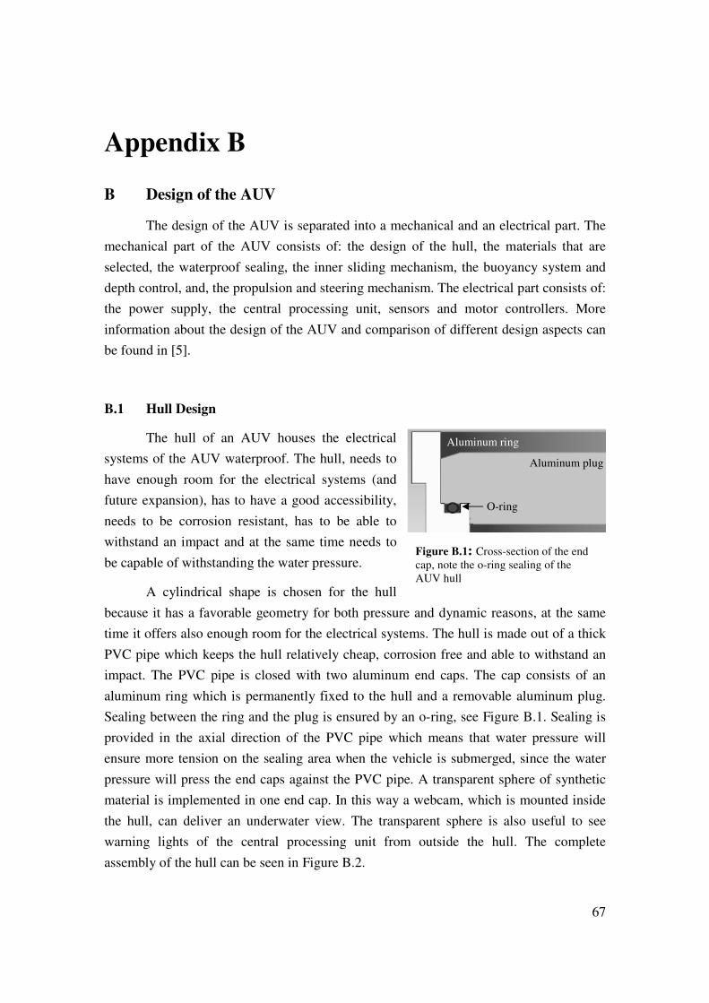
67

Appendix B

B Design of the AUV

The design of the AUV is separated into a mechanical and an electrical part. The

mechanical part of the AUV consists of: the design of the hull, the materials that are

selected, the waterproof sealing, the inner sliding mechanism, the buoyancy system and

depth control, and, the propulsion and steering mechanism. The electrical part consists of:

the power supply, the central processing unit, sensors and motor controllers. More

information about the design of the AUV and comparison of different design aspects can

be found in [5].

B.1 Hull Design

The hull of an AUV houses the electrical

systems of the AUV waterproof. The hull, needs to

have enough room for the electrical systems (and

future expansion), has to have a good accessibility,

needs to be corrosion resistant, has to be able to

withstand an impact and at the same time needs to

be capable of withstanding the water pressure.

A cylindrical shape is chosen for the hull

because it has a favorable geometry for both pressure and dynamic reasons, at the same

time it offers also enough room for the electrical systems. The hull is made out of a thick

PVC pipe which keeps the hull relatively cheap, corrosion free and able to withstand an

impact. The PVC pipe is closed with two aluminum end caps. The cap consists of an

aluminum ring which is permanently fixed to the hull and a removable aluminum plug.

Sealing between the ring and the plug is ensured by an o-ring, see Figure B.1. Sealing is

provided in the axial direction of the PVC pipe which means that water pressure will

ensure more tension on the sealing area when the vehicle is submerged, since the water

pressure will press the end caps against the PVC pipe. A transparent sphere of synthetic

material is implemented in one end cap. In this way a webcam, which is mounted inside

the hull, can deliver an underwater view. The transparent sphere is also useful to see

warning lights of the central processing unit from outside the hull. The complete

assembly of the hull can be seen in Figure B.2.

Figure B.1: Cross-section of the end

cap, note the o-ring sealing of the

AUV hull

O-ring

Aluminum plug

Aluminum ring

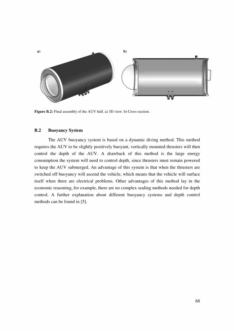
68

Figure B.2: Final assembly of the AUV hull. a) 3D view. b) Cross-section.

B.2 Buoyancy System

The AUV buoyancy system is based on a dynamic diving method. This method

requires the AUV to be slightly positively buoyant, vertically mounted thrusters will then

control the depth of the AUV. A drawback of this method is the large energy

consumption the system will need to control depth, since thrusters must remain powered

to keep the AUV submerged. An advantage of this system is that when the thrusters are

switched off buoyancy will ascend the vehicle, which means that the vehicle will surface

itself when there are electrical problems. Other advantages of this method lay in the

economic reasoning, for example, there are no complex sealing methods needed for depth

control. A further explanation about different buoyancy systems and depth control

methods can be found in [5].

a) b)

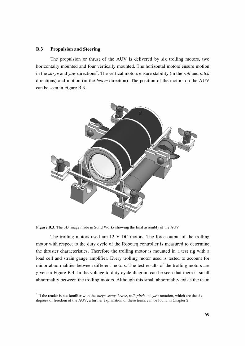
69

B.3 Propulsion and Steering

The propulsion or thrust of the AUV is delivered by six trolling motors, two

horizontally mounted and four vertically mounted. The horizontal motors ensure motion

in the surge and yaw directions*. The vertical motors ensure stability (in the roll and pitch

directions) and motion (in the heave direction). The position of the motors on the AUV

can be seen in Figure B.3.

Figure B.3: The 3D image made in Solid Works showing the final assembly of the AUV

The trolling motors used are 12 V DC motors. The force output of the trolling

motor with respect to the duty cycle of the Roboteq controller is measured to determine

the thruster characteristics. Therefore the trolling motor is mounted in a test rig with a

load cell and strain gauge amplifier. Every trolling motor used is tested to account for

minor abnormalities between different motors. The test results of the trolling motors are

given in Figure B.4. In the voltage to duty cycle diagram can be seen that there is small

abnormality between the trolling motors. Although this small abnormality exists the team

* If the reader is not familiar with the surge, sway, heave, roll, pitch and yaw notation, which are the six

degrees of freedom of the AUV, a further explanation of these terms can be found in Chapter 2.

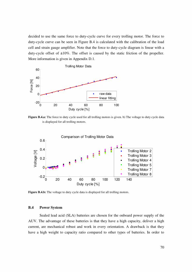
70

decided to use the same force to duty-cycle curve for every trolling motor. The force to

duty-cycle curve can be seen in Figure B.4 is calculated with the calibration of the load

cell and strain gauge amplifier. Note that the force to duty-cycle diagram is linear with a

duty-cycle offset of ±10%. The offset is caused by the static friction of the propeller.

More information is given in Appendix D.1.

0 20 40 60 80 100-20

0

20

40

60Trolling Motor Data

Duty cycle [%]

Forc

e [

N]

raw data

linear fitting

Figure B.4.a: The force to duty cycle used for all trolling motors is given. b) The voltage to duty cycle data

is displayed for all trolling motors.

0 20 40 60 80 100 120 140-0.2

0

0.2

0.4

0.6Comparison of Trolling Motor Data

Duty cycle [%]

Volt

age [

V]

Trolling Motor 2

Trolling Motor 3

Trolling Motor 4

Trolling Motor 5

Trolling Motor 7

Trolling Motor 8

Figure B.4.b: The voltage to duty cycle data is displayed for all trolling motors.

B.4 Power System

Sealed lead acid (SLA) batteries are chosen for the onboard power supply of the

AUV. The advantage of these batteries is that they have a high capacity, deliver a high

current, are mechanical robust and work in every orientation. A drawback is that they

have a high weight to capacity ratio compared to other types of batteries. In order to

71

supply enough current five batteries are parallel connected on an aluminum bus, see

Figure B.5. The AUV has three different battery compartments, one in the main hull and

two external tube battery compartments. Every compartment has 5 parallel connected

batteries. The benefit of using two tube battery compartments is that, when operating in

field, it is easier to interchange the batteries. The two tube battery compartments are used

to power the trolling motors and the main hull battery is used to power the onboard

electrical equipment. The SLA battery from Exide Powergard delivers 12 V and has a 12

AH@10 hrs current.

Figure B.5: Five parallel connected batteries which together form one battery compartment housed in an

aluminum bus.

B.5 Central Processing Unit

The central processing unit in the AUV is responsible for accessing sensors,

processing data and setting control outputs. An ADM Sempron 3000+ processor and

Asus M2N-PV motherboard are used to form this central processing unit, see Figure B.6.

This processing unit delivers adequate processing power, has enough connection ports for

the diverse range of peripherals and has an ethernet module for a remote control

connection.

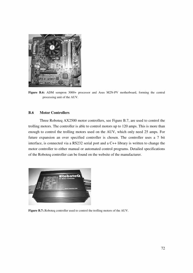
72

Figure B.6: ADM sempron 3000+ processor and Asus M2N-PV motherboard, forming the central

processing unit of the AUV.

B.6 Motor Controllers

Three Roboteq AX2500 motor controllers, see Figure B.7, are used to control the

trolling motors. The controller is able to control motors up to 120 amps. This is more than

enough to control the trolling motors used on the AUV, which only need 25 amps. For

future expansion an over specified controller is chosen. The controller uses a 7 bit

interface, is connected via a RS232 serial port and a C++ library is written to change the

motor controller to either manual or automated control programs. Detailed specifications

of the Roboteq controller can be found on the website of the manufacturer.

Figure B.7:.Roboteq controller used to control the trolling motors of the AUV.

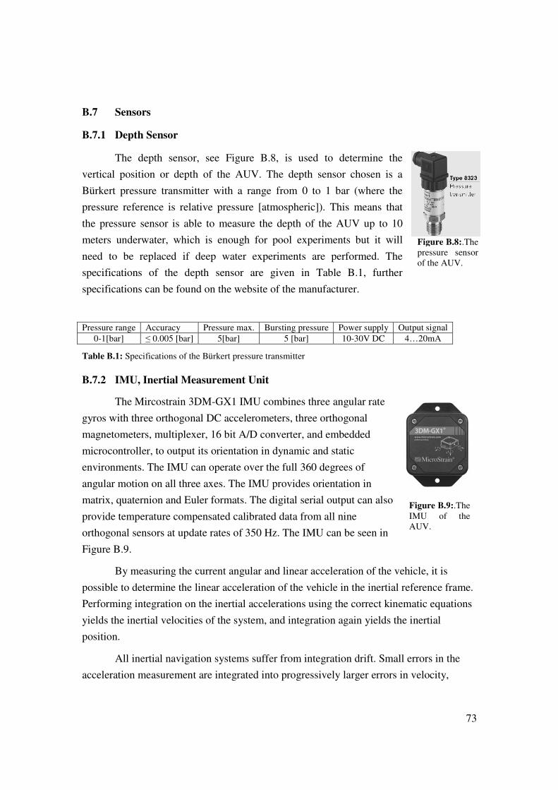
73

B.7 Sensors

B.7.1 Depth Sensor

The depth sensor, see Figure B.8, is used to determine the

vertical position or depth of the AUV. The depth sensor chosen is a

Bürkert pressure transmitter with a range from 0 to 1 bar (where the

pressure reference is relative pressure [atmospheric]). This means that

the pressure sensor is able to measure the depth of the AUV up to 10

meters underwater, which is enough for pool experiments but it will

need to be replaced if deep water experiments are performed. The

specifications of the depth sensor are given in Table B.1, further

specifications can be found on the website of the manufacturer.

Pressure range Accuracy Pressure max. Bursting pressure Power supply Output signal

0-1[bar] ≤ 0.005 [bar] 5[bar] 5 [bar] 10-30V DC 4…20mA

Table B.1: Specifications of the Bürkert pressure transmitter

B.7.2 IMU, Inertial Measurement Unit

The Mircostrain 3DM-GX1 IMU combines three angular rate

gyros with three orthogonal DC accelerometers, three orthogonal

magnetometers, multiplexer, 16 bit A/D converter, and embedded

microcontroller, to output its orientation in dynamic and static

environments. The IMU can operate over the full 360 degrees of

angular motion on all three axes. The IMU provides orientation in

matrix, quaternion and Euler formats. The digital serial output can also

provide temperature compensated calibrated data from all nine

orthogonal sensors at update rates of 350 Hz. The IMU can be seen in

Figure B.9.

By measuring the current angular and linear acceleration of the vehicle, it is

possible to determine the linear acceleration of the vehicle in the inertial reference frame.

Performing integration on the inertial accelerations using the correct kinematic equations

yields the inertial velocities of the system, and integration again yields the inertial

position.

All inertial navigation systems suffer from integration drift. Small errors in the

acceleration measurement are integrated into progressively larger errors in velocity,

Figure B.8:.The

pressure sensor

of the AUV.

Figure B.9:.The

IMU of the

AUV.

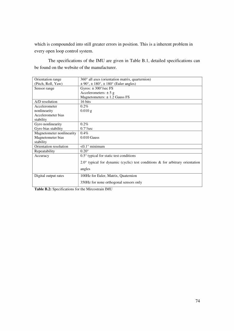
74

which is compounded into still greater errors in position. This is a inherent problem in

every open loop control system.

The specifications of the IMU are given in Table B.1, detailed specifications can

be found on the website of the manufacturer.

Orientation range

(Pitch, Roll, Yaw)

360° all axes (orientation matrix, quarternion)

± 90°, ± 180°, ± 180° (Euler angles)

Sensor range Gyros: ± 300°/sec FS

Accelerometers: ± 5 g

Magnetometers: ± 1.2 Gauss FS

A/D resolution 16 bits

Accelerometer

nonlinearity

Accelerometer bias

stability

0.2%

0.010 g

Gyro nonlinearity

Gyro bias stability

0.2%

0.7°/sec

Magnetometer nonlinearity

Magnetometer bias

stability

0.4%

0.010 Gauss

Orientation resolution <0.1° minimum

Repeatability 0.20°

Accuracy 0.5° typical for static test conditions

2.0° typical for dynamic (cyclic) test conditions & for arbitrary orientation

angles

Digital output rates 100Hz for Euler, Matrix, Quaternion

350Hz for none orthogonal sensors only

Table B.2: Specifications for the Mircostrain IMU

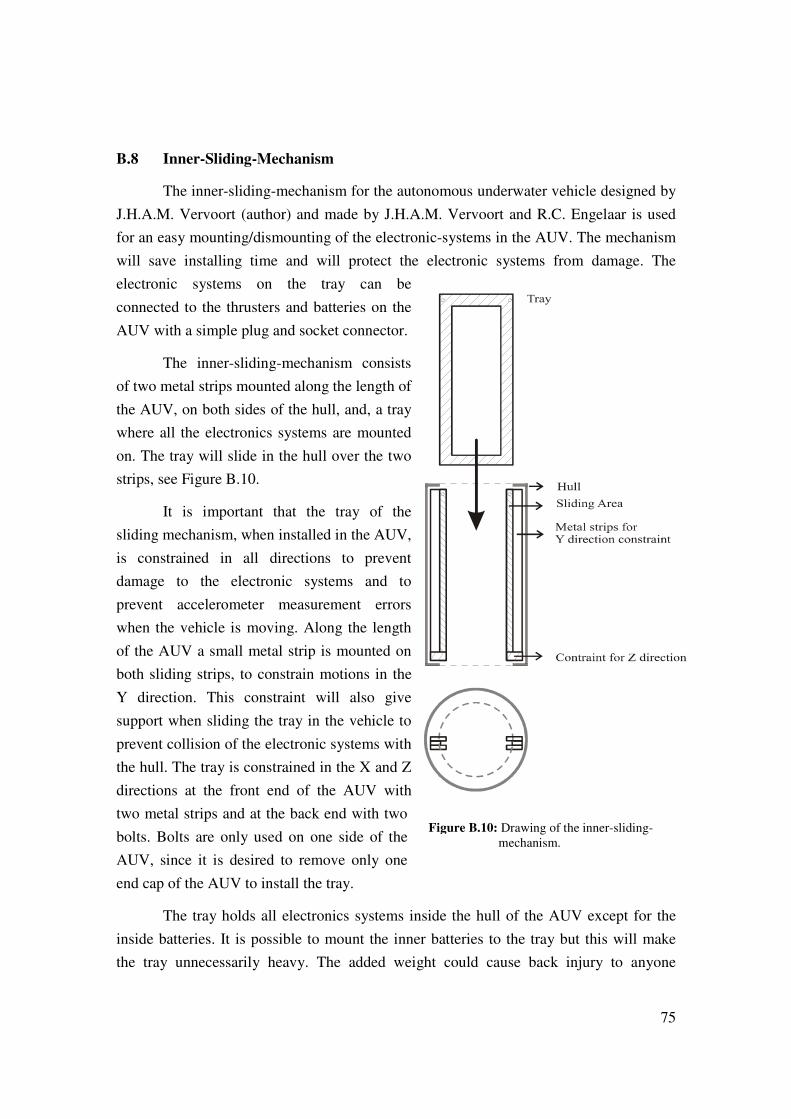
75

B.8 Inner-Sliding-Mechanism

The inner-sliding-mechanism for the autonomous underwater vehicle designed by

J.H.A.M. Vervoort (author) and made by J.H.A.M. Vervoort and R.C. Engelaar is used

for an easy mounting/dismounting of the electronic-systems in the AUV. The mechanism

will save installing time and will protect the electronic systems from damage. The

electronic systems on the tray can be

connected to the thrusters and batteries on the

AUV with a simple plug and socket connector.

The inner-sliding-mechanism consists

of two metal strips mounted along the length of

the AUV, on both sides of the hull, and, a tray

where all the electronics systems are mounted

on. The tray will slide in the hull over the two

strips, see Figure B.10.

It is important that the tray of the

sliding mechanism, when installed in the AUV,

is constrained in all directions to prevent

damage to the electronic systems and to

prevent accelerometer measurement errors

when the vehicle is moving. Along the length

of the AUV a small metal strip is mounted on

both sliding strips, to constrain motions in the

Y direction. This constraint will also give

support when sliding the tray in the vehicle to

prevent collision of the electronic systems with

the hull. The tray is constrained in the X and Z

directions at the front end of the AUV with

two metal strips and at the back end with two

bolts. Bolts are only used on one side of the

AUV, since it is desired to remove only one

end cap of the AUV to install the tray.

The tray holds all electronics systems inside the hull of the AUV except for the

inside batteries. It is possible to mount the inner batteries to the tray but this will make

the tray unnecessarily heavy. The added weight could cause back injury to anyone

Figure B.10: Drawing of the inner-sliding-

mechanism.

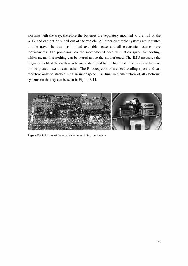
76

working with the tray, therefore the batteries are separately mounted to the hull of the

AUV and can not be slided out of the vehicle. All other electronic systems are mounted

on the tray. The tray has limited available space and all electronic systems have

requirements. The processors on the motherboard need ventilation space for cooling,

which means that nothing can be stored above the motherboard. The IMU measures the

magnetic field of the earth which can be disrupted by the hard disk drive so these two can

not be placed next to each other. The Roboteq controllers need cooling space and can

therefore only be stacked with an inner space. The final implementation of all electronic

systems on the tray can be seen in Figure B.11.

Figure B.11: Picture of the tray of the inner sliding mechanism.

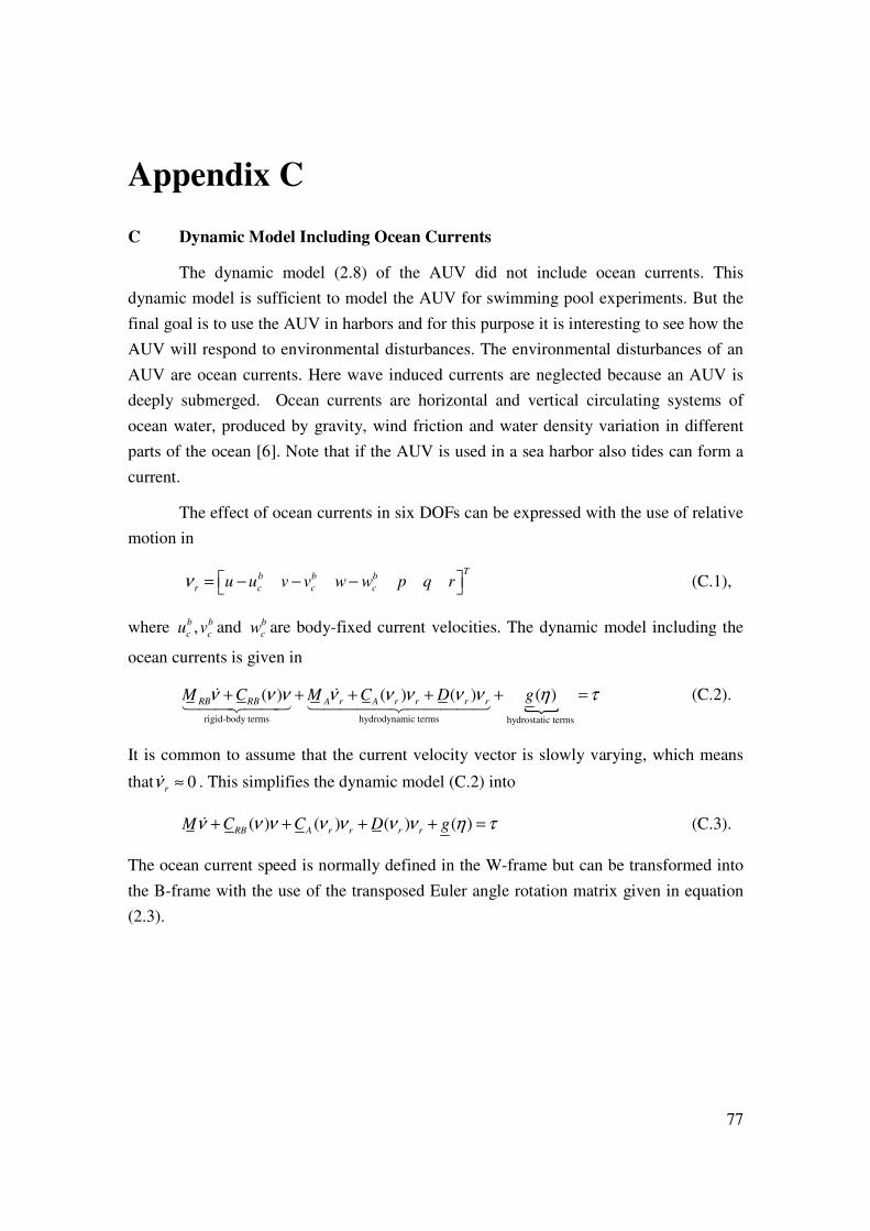
77

Appendix C

C Dynamic Model Including Ocean Currents

The dynamic model (2.8) of the AUV did not include ocean currents. This

dynamic model is sufficient to model the AUV for swimming pool experiments. But the

final goal is to use the AUV in harbors and for this purpose it is interesting to see how the

AUV will respond to environmental disturbances. The environmental disturbances of an

AUV are ocean currents. Here wave induced currents are neglected because an AUV is

deeply submerged. Ocean currents are horizontal and vertical circulating systems of

ocean water, produced by gravity, wind friction and water density variation in different

parts of the ocean [6]. Note that if the AUV is used in a sea harbor also tides can form a

current.

The effect of ocean currents in six DOFs can be expressed with the use of relative

motion in

T

b b b

r c c cu u v v w w p q rν = − − − (C.1),

where ,b b

c cu v and b

cw are body-fixed current velocities. The dynamic model including the

ocean currents is given in

{rigid-body terms hydrodynamic terms hydrostatic terms

( ) ( ) ( ) ( )RB RB A r A r r r rM C M C D gν ν ν ν ν ν ν ν η τ+ + + + + =& &1442443 14444244443

(C.2).

It is common to assume that the current velocity vector is slowly varying, which means

that 0rν ≈& . This simplifies the dynamic model (C.2) into

( ) ( ) ( ) ( )RB A r r r rM C C D gν ν ν ν ν ν ν η τ+ + + + =& (C.3).

The ocean current speed is normally defined in the W-frame but can be transformed into

the B-frame with the use of the transposed Euler angle rotation matrix given in equation

(2.3).

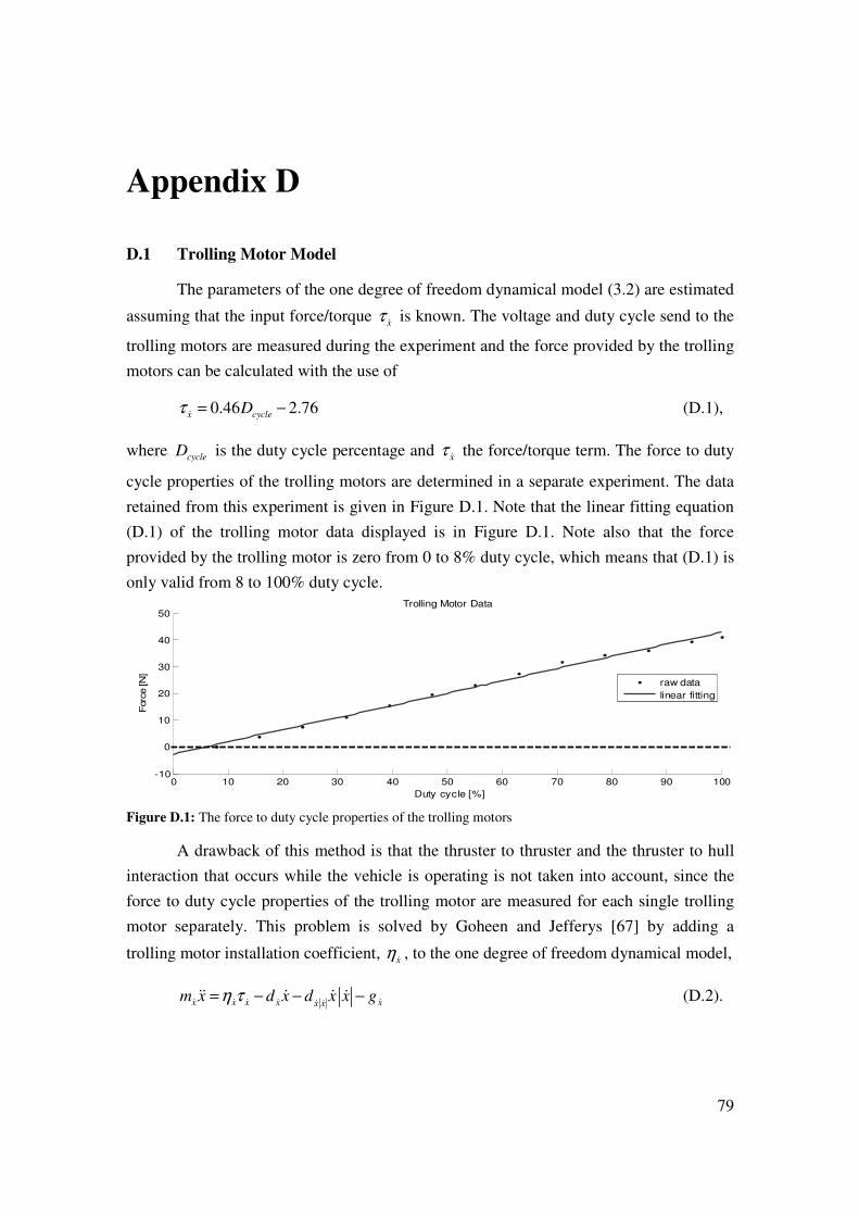
79

Appendix D

D.1 Trolling Motor Model

The parameters of the one degree of freedom dynamical model (3.2) are estimated

assuming that the input force/torque xτ & is known. The voltage and duty cycle send to the

trolling motors are measured during the experiment and the force provided by the trolling

motors can be calculated with the use of

0.46 2.76x cycleDτ = −& (D.1),

where cycleD is the duty cycle percentage and xτ & the force/torque term. The force to duty

cycle properties of the trolling motors are determined in a separate experiment. The data

retained from this experiment is given in Figure D.1. Note that the linear fitting equation

(D.1) of the trolling motor data displayed is in Figure D.1. Note also that the force

provided by the trolling motor is zero from 0 to 8% duty cycle, which means that (D.1) is

only valid from 8 to 100% duty cycle.

Figure D.1: The force to duty cycle properties of the trolling motors

A drawback of this method is that the thruster to thruster and the thruster to hull

interaction that occurs while the vehicle is operating is not taken into account, since the

force to duty cycle properties of the trolling motor are measured for each single trolling

motor separately. This problem is solved by Goheen and Jefferys [67] by adding a

trolling motor installation coefficient, xη & , to the one degree of freedom dynamical model,

x x x x xx x

m x d x d x x gη τ= − − −& & & & && &&& & & & (D.2).

0 10 20 30 40 50 60 70 80 90 100-10

0

10

20

30

40

50Trolling Motor Data

Duty cycle [%]

Forc

e [N

]

raw data

linear fitting

80

In this way the reduction in the trolling motor force can be taken into account to have an

even more accurate model. The installation coefficient can be tuned during the

underwater experiments, but for now the assumption is made that xη & is equal to one.

Another assumption made in the trolling motor model is that the trolling motor is

able to provide the same power running forwards and backwards. The difference in

forward and backward power can be implemented into the model by choosing a different

trolling motor efficiency coefficient for the forward and backward direction, but for now

it is assumed that the forward and backward power is the same.

D.2 Static Experiment, Identification of the Damping Terms

In the static experiment a constant force/torque is provided by the trolling motors

in the right mapping for the specific degree of freedom. The experiment starts when the

steady state condition is reached, where velocity is constant and the acceleration zero.

Under steady state conditions the dynamic model (3.2) changes into

0 , 0x x xx xd x d x x g Where xτ= − − − =& & && &

& & & && (D.3).

Note that 0x =&& , which means that the xm& term is canceled out off the dynamic model.

The force/torque term xτ & and the gravitational and buoyancy term xg & are fully known

parts of (D.3), for a proper least square estimation (D.3) is rewritten into

[ ] {T

x x

y X

g x x xε

θ

τ α β ε− = + & & & & &123 1424314243

(D.4).

The unknown parameters of D.4 are the linear and quadratic drag coefficients, which can

be estimated with use of the least square technique. For an explanation of the least square

technique and the application of the least square technique on the dynamical model (D.4)

one is referred to Appendix E.

D.3 Dynamic Experiment, Identification of the Mass and Inertia Term

In the dynamic experiment a sinusoidal force/torque in one specific degree of

freedom is applied to the AUV. The only unknown parameter left is the inertia and mass

term, xm& , since the drag parameters are already identified in the static experiment. The

one degree of freedom dynamic model (4.2) changes into

81

{{x x x xx x

Xy

d x d x x g x m

θ

τ ε− − − = +& & & && && & & &&

144424443 (D.5),

where the known terms, y, are formed by xτ & ,

xg & ,xd & and

x xd & &

, and the unknown term,θ , is

xm& . The unknown term can be estimated with the use of the least square technique which

is explained in Appendix E.

83

Appendix E

E.1 Least Squares Technique

The least squares (LS) technique is a frequently used approach to solve

(approximate) over-determined or inexactly specified systems of equations [68]. Instead

of solving the equations exactly the LS technique minimizes the sum of residuals. This

subsection explains the LS technique, gives the normal equations in matrix form (which

are needed to estimate the unknown parameter) and provides the standard deviation of the

estimated parameters and parameter error equations. More information about the LS

technique can be found in [17, 45, 51, 56, 66, 68].

Let t be the independent variable and let y(t) denote an unknown function of t that

needs to be approximated. Assume that there are m observations, i.e. values of y

measured at specified values of t,

( ), 1,...,i iy y t i m= = (E.1).

The idea is to model y(t) by a linear combination of n basis functions,

1 1( ) ( ) ... ( )n ny t t tθ φ θ φ≈ + + (E.2).

The design matrix, , ( )i j j ix tφ= , is a rectangular matrix of order m by n, which normally

has more rows than columns. The matrix-notation of E.2 is given by

y Xθ≈ (E.3).

After an experiment there are more equations than unknowns, so the system is

over-determined, which means that the system can not be solved exactly. The goal of the

least square estimation is now to find the values ˆjθ , which fit the equations best. In other

words, it has to find the minimum possible value of the sum of squares of the residuals.

The residuals are the differences between the observations and the model, given by

,

1

ˆ , 1,...,n

i i j i jr y x i mθ= − =∑ (E.4)

or in matrix notation given by

ˆr y Xθ= − (E.5)

The least square method minimizes the sum of squares of the residuals, which is given by

84

2 2

1

m

ir r=∑ (E.6)

2r is minimized when its gradient with respect to each parameter is equal to zero, this is

defined by

2

,

2 0, i 1,..., , 1,...,ˆ ˆ

Where: ˆ

mi

i

ij j

ii j

j

r rr m j n

rx

θ θ

θ

∂ ∂= = = =

∂ ∂

∂= −

∂

∑ (E.7).

Substitution of (E.4) in (E.7) gives

2

, ,

1 1

ˆ2 0 ˆ

m n

i j i j i j

i jj

rx y xθ

θ = =

∂= − − =

∂ ∑ ∑ (E.8)

and rearrangement gives

, , ,

1 1 1

ˆm n m

i j i j j i j i

i j i

x x x yθ= = =

=∑∑ ∑ (E.9),

which form the normal equations of the least square estimation. The normal equations

written in matrix notation are given by

( ) ˆT TX X X yθ = (E.10).

So the estimate of the parameters can be found from

( )1ˆ T T

X X X yθ−

= (E.11).

Note that to invert the normal equations matrix, the TX X matrix needs to be well-

conditioned and positive definite, the TX X matrix has to have full rank. The standard

deviation of this estimated parameter is computed [17] with

( )( )12ˆ diag t

X Xθ εσ σ−

= (E.12),

where 2σ̂ is the estimated Gaussian zero mean measurement noise variance, which is

defined by

85

( ) ( )2

ˆ ˆ

ˆdim( ) dim( )

T

Y X Y X

Yε

θ θσ

θ

− −=

− (E.13).

The standard deviation and estimate of the parameters can be used to determine the

parameter relative percentile error, which is defined by

ˆ100

ˆθσ

ςθ

= (E.14),

where Indiveri [17] gives the following explanation for statistically insignificancy:

“If the parameter variance is too large the parameter itself is said to be statistically

insignificant and it might just as well be put to zero. More precisely given the two

hypothesis 0h and 1h :

0

1 0

1

: 0such that ( | )

: 0

i

i

hp accept h h true

h

θα

θ

==

≠

Being iθ normaly distributed with the standard deviation iθσ and α some arbitrary

constant (usually 5%), the hypothesis is accepted if

ˆ

( )ˆ

i

i

cθ

θα

σ> being 1.96c = if 5%α = .

In percentile notation it can be said that if the parameter relative percentile error ς is

larger than 51.02%, see 4.19, there is a 95% confidence limit that the parameter itself is

statistically insignificant and the hypothesis 0 : 0ih θ = is better to be accepted.

ˆ 100100 % 51.02%

ˆ 1.96

θσ

ςθ

> → > (E.15)”

E.2 Least Square Applied

The LS technique explained above can be applied on the one degree of freedom

dynamical model (4.2), to estimate the inertia and drag parameters, ,x xm d& & and x x

d & & for

each degree of freedom. The one degree of freedom dynamical model can be rewritten

into

( )x xx g x x xγ τ α β ε= − + + +& &&& & & & (E.16),

where ,α β andγ are defined by

86

x

x

d

mα = − &

&

(E.17),

x x

x

d

mβ = −

& &

&

(E.18)

and

1

xmγ =

&

(E.19),

Respectively, and ε is a measurement noise term. Note that xm& defines the rigid body

and added mass, for : x usurge m m X= −& & , for : x wheave m m Z= −& & and for

: x ryaw m m N= −& & . Note also that xg & is zero for the surge and yaw degrees of freedom.

The dynamic model (E.16) rewritten into a matrix form gives

[ ]T

x xx x x x gτ α β γ ε= − + & &&& & & & (E.20).

If a decoupled experiment is run with N samples, (E.20) expands to N rows as can be

seen in

{ {

1 ,1 ,11 1 1 1 11

2 ,2 ,22 2 2 2 22

, ,

x x

x x

x x

x x x gx

x x x gx

x x x gx

y X

τ α β γ ε

τ α β γ ε

τ α β γ εΝ Ν ΝΝ Ν Ν Ν ΝΝ

− − = +

−

=

& &

& &

& &

& & &&&

& & &&&

M M MM M M M M

& & &&&144244314444244443

θ ε⋅ +

(E.21),

which now has the same form as E.3. Now the LS estimation can be applied on E.21 to

estimate the vector of unknownsθ .

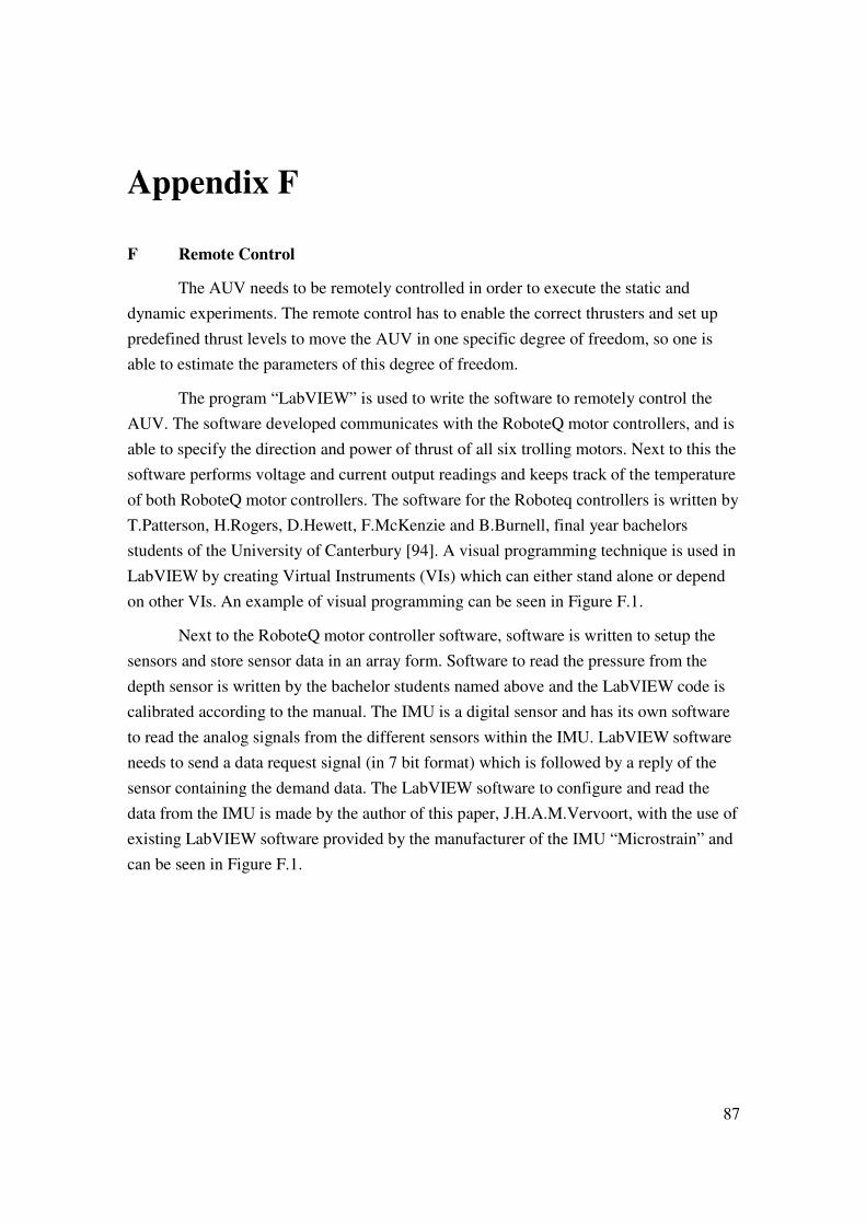
87

Appendix F

F Remote Control

The AUV needs to be remotely controlled in order to execute the static and

dynamic experiments. The remote control has to enable the correct thrusters and set up

predefined thrust levels to move the AUV in one specific degree of freedom, so one is

able to estimate the parameters of this degree of freedom.

The program “LabVIEW” is used to write the software to remotely control the

AUV. The software developed communicates with the RoboteQ motor controllers, and is

able to specify the direction and power of thrust of all six trolling motors. Next to this the

software performs voltage and current output readings and keeps track of the temperature

of both RoboteQ motor controllers. The software for the Roboteq controllers is written by

T.Patterson, H.Rogers, D.Hewett, F.McKenzie and B.Burnell, final year bachelors

students of the University of Canterbury [94]. A visual programming technique is used in

LabVIEW by creating Virtual Instruments (VIs) which can either stand alone or depend

on other VIs. An example of visual programming can be seen in Figure F.1.

Next to the RoboteQ motor controller software, software is written to setup the

sensors and store sensor data in an array form. Software to read the pressure from the

depth sensor is written by the bachelor students named above and the LabVIEW code is

calibrated according to the manual. The IMU is a digital sensor and has its own software

to read the analog signals from the different sensors within the IMU. LabVIEW software

needs to send a data request signal (in 7 bit format) which is followed by a reply of the

sensor containing the demand data. The LabVIEW software to configure and read the

data from the IMU is made by the author of this paper, J.H.A.M.Vervoort, with the use of

existing LabVIEW software provided by the manufacturer of the IMU “Microstrain” and

can be seen in Figure F.1.

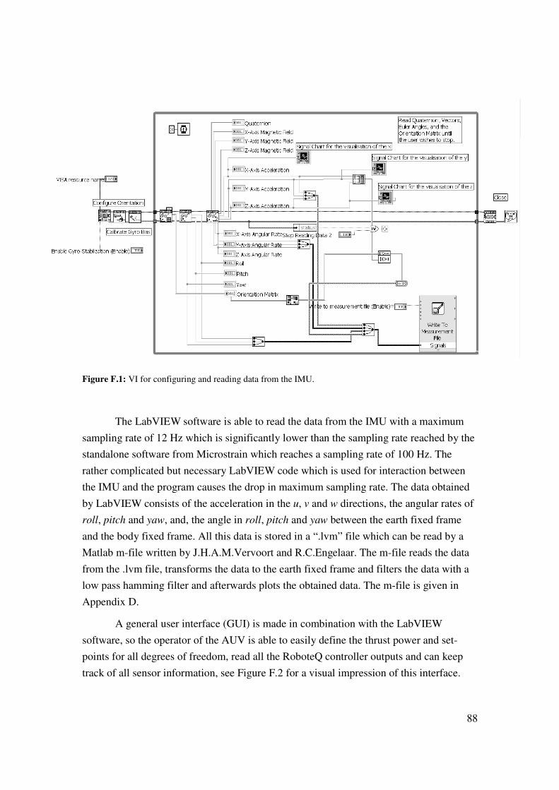
88

Figure F.1: VI for configuring and reading data from the IMU.

The LabVIEW software is able to read the data from the IMU with a maximum

sampling rate of 12 Hz which is significantly lower than the sampling rate reached by the

standalone software from Microstrain which reaches a sampling rate of 100 Hz. The

rather complicated but necessary LabVIEW code which is used for interaction between

the IMU and the program causes the drop in maximum sampling rate. The data obtained

by LabVIEW consists of the acceleration in the u, v and w directions, the angular rates of

roll, pitch and yaw, and, the angle in roll, pitch and yaw between the earth fixed frame

and the body fixed frame. All this data is stored in a “.lvm” file which can be read by a

Matlab m-file written by J.H.A.M.Vervoort and R.C.Engelaar. The m-file reads the data

from the .lvm file, transforms the data to the earth fixed frame and filters the data with a

low pass hamming filter and afterwards plots the obtained data. The m-file is given in

Appendix D.

A general user interface (GUI) is made in combination with the LabVIEW

software, so the operator of the AUV is able to easily define the thrust power and set-

points for all degrees of freedom, read all the RoboteQ controller outputs and can keep

track of all sensor information, see Figure F.2 for a visual impression of this interface.

89

Figure F.2: The GUI developed to remotely control the AUV.

91

Appendix G

G.1 Input-output linearization

The choice for the state feedback control law u given in (4.7) can be confirmed by the

input-output linearization of the state equation (4.6), which is already in normal form. For

the input-output linearization it is important to know the relative degree of the nonlinear

system. The relative degree ρ is the number of times the output y has to be differentiated

before the input u appears. The relative degree can be determined with the use of a

definition defined by H.K.Khalil [74], see Appendix G.2, note that this definition makes

use of Lie Derivatives. If the relative degree of the nonlinear system is known then the

state feedback control u can be determined with

1

1( )

( )f

g f

u L h x vL L h x

ρ

ρ − = − + (G.1),

where ( )

( ) ( )f

g f

L hL L h x g x

x

∂=

∂with ( )

f

hL h f x

x

∂=

∂ and

( )2 ( ) ( )

f

f

L hL h x f x

x

∂=

∂. Here

the notation of H.K.Khalil is used in combination with the Lie Derivatives.

The relative degree of the state equation is determined by the differentiation of the

output, which results in

1y x= (G.2.a),

1 2y x x= =& & (G.2.b),

2 2 2 2y x ax bx x du= = − − +&& & (G.2.c),

where the input u appears in y&& , 2ρ = , which also verified by the definition of H.K.Khalil

in Appendix G.3.

With the relative degree known the state feedback control law u can be

determined with the use of (G.1), which gives

( ) ( )2

2 2 2

1 1( )

( )f

g f

u L h x v ax bx x vL L h x d

= − + = + + (G.3),

where ( )g fL L h x d= , 2fL h x= and 2

2 2 2( )fL h x ax bx x= − − . The state feedback control

law (G.3) is similar to (4.7) and reduces the input-output map to y v=&& . This means that

the state equation (4.6) is indeed input-output linearizable. Note that the relative degree is

92

similar to the number of states, nρ = , which means that there are no internal dynamics.

The system has no zero dynamics and by default is said to be minimum phase [73 74].

G.2 The definition of Khalil

[Khalil [74], “Nonlinear Systems”, Third edition, Definition 13.2]

The nonlinear system is said to have a relative degree ρ , 1 nρ≤ ≤ , in a region

0D D⊂ if

1 1( ) 0, 1, 2, , 1; ( ) 0i

g f g fL L h x i L L h x

ρρ− −= = − ≠K (G.4)

for all 0x D∈ �

G.3 The definition of Khalil applied

[Khalil [74], “Nonlinear Systems”, Third edition, Definition 13.2]

The definition of Khalil applied to calculate the relative degree of the state

equation (4.6):

1

2

( ) ( ) ( ) 0, 1 1 i

g f g

h hL L h x L h x g x d i

x xρ− ∂ ∂

= = = = = − =∂ ∂

(G.5)

( )1 ( ) ( ) ( ) 0, 2

f

g f g f

L hL L h x L L h x g x d

x

ρ ρ−∂

= = = ≠ =∂

(G.6)

G.4 Eigenvalue determination

Calculations to prove that (4.13) is only Hurwits for 1 0k > and 2 0k > :

det( ) 0A KB Iλ− − = (G.7)

Where 1 2 1 2

0 0 0 10 1

0 0A BK

k k k k

− = − = − −

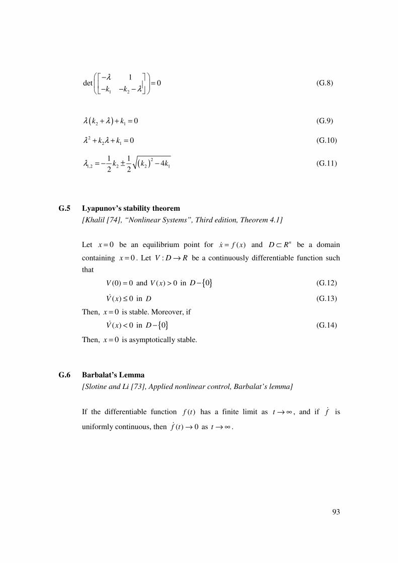
93

1 2

1det 0

k k

λ

λ

− = − − −

(G.8)

( )2 1 0k kλ λ+ + = (G.9)

2

2 1 0k kλ λ+ + = (G.10)

( )2

1,2 2 2 1

1 14

2 2k k kλ = − ± − (G.11)

G.5 Lyapunov’s stability theorem

[Khalil [74], “Nonlinear Systems”, Third edition, Theorem 4.1]

Let 0x = be an equilibrium point for ( )x f x=& and nD R⊂ be a domain

containing 0x = . Let :V D R→ be a continuously differentiable function such

that

(0) 0V = and ( ) 0V x > in { }0D − (G.12)

( ) 0V x ≤& in D (G.13)

Then, 0x = is stable. Moreover, if

( ) 0V x <& in { }0D − (G.14)

Then, 0x = is asymptotically stable. �

G.6 Barbalat’s Lemma

[Slotine and Li [73], Applied nonlinear control, Barbalat’s lemma]

If the differentiable function ( )f t has a finite limit as t → ∞ , and if f& is

uniformly continuous, then ( ) 0f t →& as t → ∞ . �

94

G.7 Lyapunov-Like Lemma

[Slotine and Li [73], Applied nonlinear control, lemma 4.3]

If a scalar function ( ),V x t satisfies the following conditions:

1. ( ),V x t is lower bounded

2. ( ),V x t& is negative semi-definite

3. ( ),V x t& is uniformly continuous in time

then ( ), 0V x t →& as t → ∞ . �

G.8 [A.A.J.Lefeber [83], Corollary 2.3.4]

Consider the system

( )( )rx A r t x Bu= +& (G.15)

y Cx= (G.16)

Where ( )rA r is continuous, (0) 0A = , :rr →� � continuous. Assume that for all

0s ≠ the pair ( )( ),A s B is controllable (respectively the pair ( )( ),A s C is observable).

If ( )rr t is bounded, Lipschitz and constants 0cδ > and 0ε > exist such that 0,t∀ ≥

: cs t s tδ∃ − ≤ ≤ such that rr ε≥ then the system in 7.41 and 7.42 is uniformly

completely controllable (respectively observable). �

95

Appendix H

H Control Techniques

H.1 PID Control

PID control or Proportional-Integral-Derivative control is a control loop feedback

mechanism, which is used to correct the error between a measured variable and a desired

reference variable (or set-point) with a corrective action. To correct, for example, the

error between the current and desired depth of the AUV by enabling the vertical thrusters.

The PID controller consists of three different parameters or gains, namely the

proportional, integral and derivative gain. The proportional gain determines the reaction

to the current error. The integral gain determines the reaction based on the sum of recent

errors. The derivative gain determines the reaction to the rate at which the error has been

changing. The weighted sum of these three actions is used to adjust the output, for

instance the power of the thrusters of the AUV [6 10 19]. The PID algorithm is given by

p i pu k e k e k e= + +∫ & (H.1)

Where, u is the output of the PID controller, kp is the proportional gain, ki is the integral

gain, kd is the derivative gain and e is the error signal.

The three different gains within the PID controller all have there own influence.

Enlarging the kp gain will result in a faster response of the controller, although an

excessively larger chosen proportional term will lead to instability and oscillation.

Enlarging the ki gain will imply a quicker elimination of steady state errors but the

drawback is a larger overshoot. A larger kd gain will decrease the overshoot but slows

down the response of the system and causes signal noise amplification in the

differentiation of the error which may lead to instability. The effect of increasing gains is

given in Table H.1 and can also be found in [39].

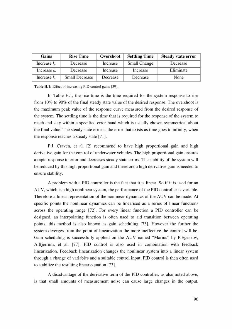
96

Gains Rise Time Overshoot Settling Time Steady state error

Increase kp Decrease Increase Small Change Decrease

Increase ki Decrease Increase Increase Eliminate

Increase kd Small Decrease Decrease Decrease None

Table H.1: Effect of increasing PID control gains [39].

In Table H.1, the rise time is the time required for the system response to rise

from 10% to 90% of the final steady state value of the desired response. The overshoot is

the maximum peak value of the response curve measured from the desired response of

the system. The settling time is the time that is required for the response of the system to

reach and stay within a specified error band which is usually chosen symmetrical about

the final value. The steady state error is the error that exists as time goes to infinity, when

the response reaches a steady state [71].

P.J. Craven, et al. [2] recommend to have high proportional gain and high

derivative gain for the control of underwater vehicles. The high proportional gain ensures

a rapid response to error and decreases steady state errors. The stability of the system will

be reduced by this high proportional gain and therefore a high derivative gain is needed to

ensure stability.

A problem with a PID controller is the fact that it is linear. So if it is used for an

AUV, which is a high nonlinear system, the performance of the PID controller is variable.

Therefore a linear representation of the nonlinear dynamics of the AUV can be made. At

specific points the nonlinear dynamics can be linearised as a series of linear functions

across the operating range [72]. For every linear function a PID controller can be

designed, an interpolating function is often used to aid transition between operating

points, this method is also known as gain scheduling [73]. However the further the

system diverges from the point of linearization the more ineffective the control will be.

Gain scheduling is successfully applied on the AUV named “Marius” by P.Egeskov,

A.Bjerrum, et al. [77]. PID control is also used in combination with feedback

linearization. Feedback linearization changes the nonlinear system into a linear system

through a change of variables and a suitable control input, PID control is then often used

to stabilize the resulting linear equation [73].

A disadvantage of the derivative term of the PID controller, as also noted above,

is that small amounts of measurement noise can cause large changes in the output.

97

Measurements are therefore filtered with a low pass filter to remove high frequency

noise. However reducing noise of the sensors (in a instrumental way) is preferred, since

low pass filtering and derivative control can cancel each other out [2].

H.2 Linear Quadratic Gaussian Controllers

The Linear Quadratic Gaussian or LQG controller assumes a linear system,

quadratic cost function and Gaussian noise. The LQG control is an optimal control

problem and tries to achieve a certain optimality criterion with a combination of a

Kalman filter, i.e. a Linear-Quadratic Estimator (LQE) and a Linear-Quadratic Regulator

(LQR) to optimize the controller [6, 34, 35].

A.Santos and R.R.Bitmead have tested a flying AUV with a LQG controller [36].

They implemented the LQG controller in a linear and nonlinear controller for the AUV.

Linear altitude control of the AUV resulted in a chattered control signal of the AUV,

which caused skidding of the vehicle. The altitude deviations are mostly caused by the

poor estimator. Nonlinear control reduced the chattering in the control, the altitude

deviations are reduced and the response is faster. An extended kalman filter (EKF) was

introduced, which was also primarily responsible for the improvements.

H.3 Fuzzy Logic Control

Fuzzy control is control with logics (sentences) rather than equations [30]. An

example of the program rules of a fuzzy logic controller:

1. If error < 0 and change in error < 0 then output = NB

2. If error < 0 and change in error = 0 then output = NM

The rules (given above) are in the if-then format and are applied in a rule based

controller. The computer is able to execute the rules and compute a control signal

depending on the measured inputs. An advantage of a fuzzy controller is that the control

strategy is stored in a natural language, which is easier to understand for a non-specialist

end-user. A disadvantage is that a non-fuzzy logic controller can be designed much more

quickly [31 32 33]. The fuzzy controller is useful when a mathematical model is not

known well or not known at all. Implementing fuzzy control on an AUV can avoid the

complex hydrodynamic modeling of the vehicle. Fuzzy logic controllers are implemented

with success on AUVs in several cases [20, 21, 22]. Note that when a mathematical

model is available the use of classical control theory is more appropriate.

98

H.4 Adaptive Control

Adaptive control is a form of non-linear control used for uncertain or time-

varying systems and it is mainly applied on systems with a known dynamic structure with

unknown constant or slowly-varying parameters [73, 74]. Adaptive control is useful for

AUV’s due to the changing dynamics in the ocean. The controller can adapt itself to

varying ocean currents or to a different vehicle mass when new equipment is installed.

According to P.J. Craven, R. Sutton, et al. [2], the most successful AUV control studies

include some form of adaptive control strategy.

J.Nie, T. Fossen et al.[22] presented a sensor-based navigation system and an

adaptive control system for shallow water UUVs. All control gains were initially set to

zero and adjusted by the adaptive control law, which resulted in accurate control of the

UUV in six degrees of freedom using the estimated position and velocity from the on-

board sensor-based navigation system. G. Antonelli, S. Chiaverini, et. al. [12] presented

experimental results of adaptive control using the AUV named “ODIN”. Other interesting

research on adaptive control is done by T. Fossen and I. Fjellstad [20], S. Sagatun and R.

Johansson [21], and, T. Fossen and S. Sagatun [23].

H.5 Sliding Mode Control

Another nonlinear control technique is Sliding Mode Control or SMC, which

leads to robust control under parameter uncertainties [73 74]. SMC is frequently used to

control AUVs and consists of a switching control law that transforms the state trajectory

of the plant onto a sliding surface. The control law is designed in such a way that the

system will diverge to the sliding surface. Afterwards the control law constrains the

system so it stays on the sliding surface where it has desired dynamics [2, 46, 70].

Interesting research on sliding mode control is performed by J. Healey and D. Lienard

[13, 26], D.B. Marco, A.J. Healey [14] and in T. Fossen and B. Foss [25].

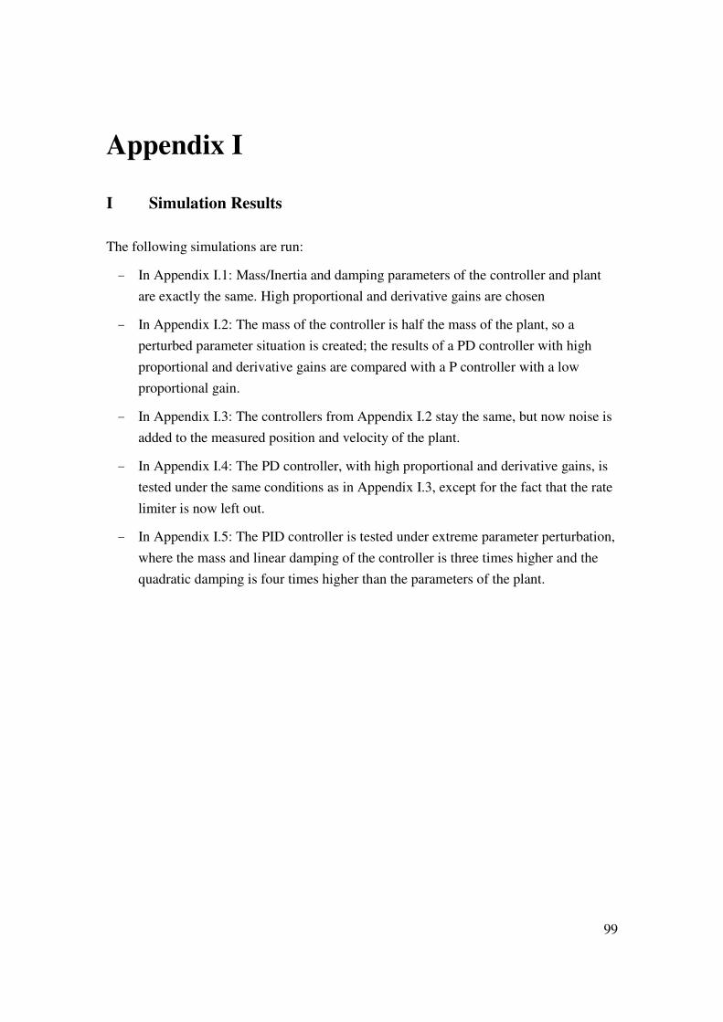
99

Appendix I

I Simulation Results

The following simulations are run:

- In Appendix I.1: Mass/Inertia and damping parameters of the controller and plant

are exactly the same. High proportional and derivative gains are chosen

- In Appendix I.2: The mass of the controller is half the mass of the plant, so a

perturbed parameter situation is created; the results of a PD controller with high

proportional and derivative gains are compared with a P controller with a low

proportional gain.

- In Appendix I.3: The controllers from Appendix I.2 stay the same, but now noise is

added to the measured position and velocity of the plant.

- In Appendix I.4: The PD controller, with high proportional and derivative gains, is

tested under the same conditions as in Appendix I.3, except for the fact that the rate

limiter is now left out.

- In Appendix I.5: The PID controller is tested under extreme parameter perturbation,

where the mass and linear damping of the controller is three times higher and the

quadratic damping is four times higher than the parameters of the plant.

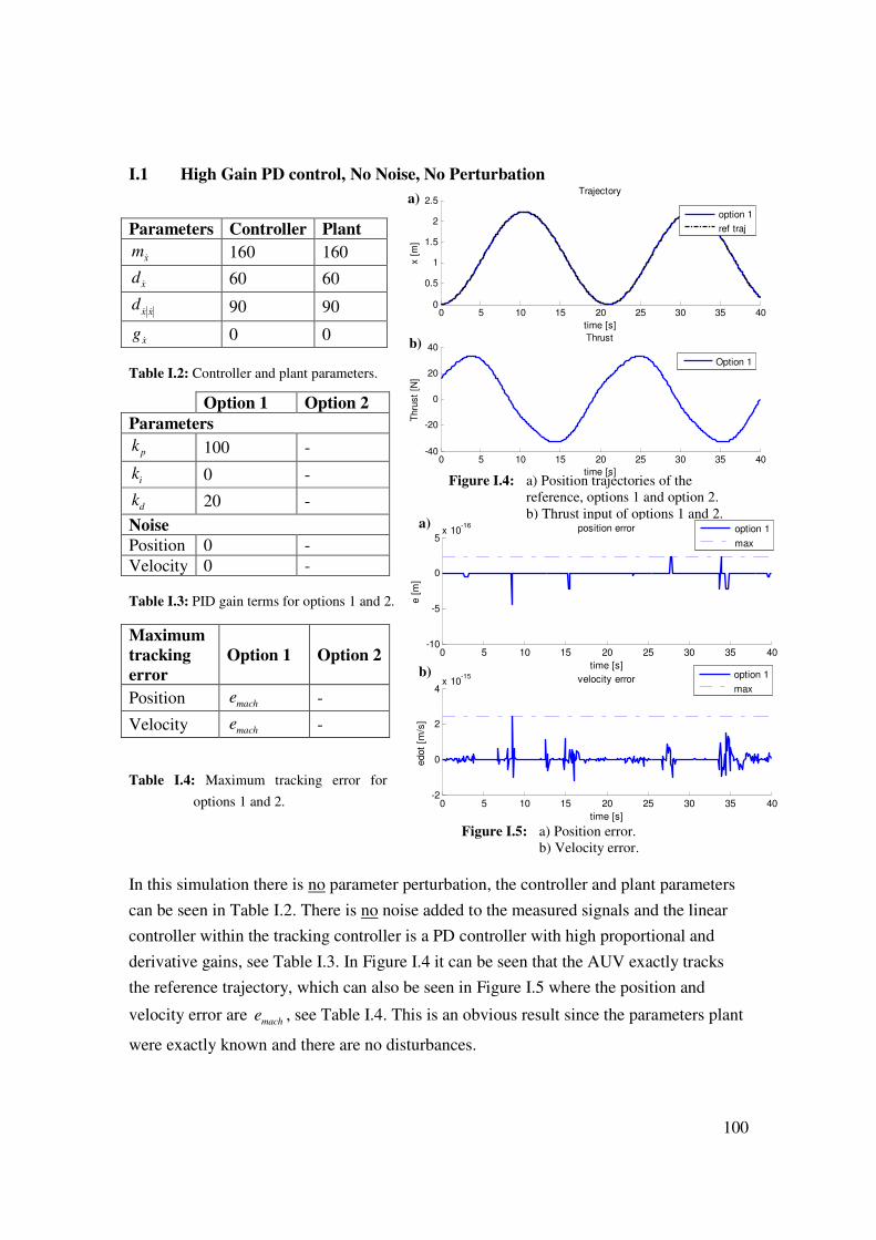
100

I.1 High Gain PD control, No Noise, No Perturbation

Table I.2: Controller and plant parameters.

Table I.3: PID gain terms for options 1 and 2.

Table I.4: Maximum tracking error for

options 1 and 2.

In this simulation there is no parameter perturbation, the controller and plant parameters

can be seen in Table I.2. There is no noise added to the measured signals and the linear

controller within the tracking controller is a PD controller with high proportional and

derivative gains, see Table I.3. In Figure I.4 it can be seen that the AUV exactly tracks

the reference trajectory, which can also be seen in Figure I.5 where the position and

velocity error are mache , see Table I.4. This is an obvious result since the parameters plant

were exactly known and there are no disturbances.


xm& 160 160

xd & 60 60

x xd & &

90 90

xg & 0 0

Option 1 Option 2

Parameters

pk

100 -

ik 0 -

dk 20 -

Noise

Position 0 -

Velocity 0 -

Maximum

tracking

error

Option 1 Option 2

Position mache -

Velocity mache -

Figure I.5: a) Position error.

b) Velocity error.

Figure I.4: a) Position trajectories of the

reference, options 1 and option 2.


0 5 10 15 20 25 30 35 40-10

-5

0

5x 10

-16

time [s]

e [

m]

position error

option 1

max

0 5 10 15 20 25 30 35 40-2

0

2

4x 10

-15

time [s]

edot

[m/s

]

velocity error

option 1

max

0 5 10 15 20 25 30 35 400

0.5

1

1.5

2

2.5

time [s]

x [

m]

Trajectory

option 1

ref traj

0 5 10 15 20 25 30 35 40-40

-20

0

20

40

time [s]

Thru

st

[N]

Thrust

Option 1

a)

b)

a)

b)

101

Figure I.7: a) Position error, b) Velocity error

I.2 Low Gain P control and High Gain PD control, No Noise, With Perturbation




options 1 and 2.

In this simulation there is parameter perturbation, the controller and plant parameters can

be seen in Table I.5. There is no noise added to the measured signals, see Table I.6. The

linear controller within the tracking controller for option one is a P controller with a low

proportional gain and for option 2 is a PD controller with high proportional and

derivative gains, the P and PD gains are shown in Table I.5. In Figure I.6 it can be seen

that control option 1 tracks the reference trajectory, with a reasonable error of 0.23 m.

However control option 2 manages to follow the trajectory with only a position error of 1

mm, which is also an obvious result since the high proportional and derivative gains will

immediately response to an error.


xm& 80 160

xd & 60 60

x xd & &

90 90

xg & 0 0

Option 1 Option 2

Parameters

pk

1 100

ik 0 0

dk 0 20

Noise

Position 0 0

Velocity 0 0

Maximum

tracking

error

Option 1

Option 2

Position 0.2323 9.999e-4

Velocity 0.1197 2.999e-4




0 5 10 15 20 25 30 35 40-1

0

1

2

3

time [s]

x [

m]

Trajectory

option 1

option 2

ref traj

0 5 10 15 20 25 30 35 40-100

-50

0

50

time [s]

Thru

st

[N]

Thrust

Option 1

Option 2

0 5 10 15 20 25 30 35 40-0.4

-0.2

0

0.2

0.4

time [s]

e [

m]

position error

option 1

max

option 2

max

0 5 10 15 20 25 30 35 40-0.2

-0.1

0

0.1

0.2

time [s]

edot

[m/s

]

velocity error

option 1

max

option 2

max

a)

b)

a)

b)

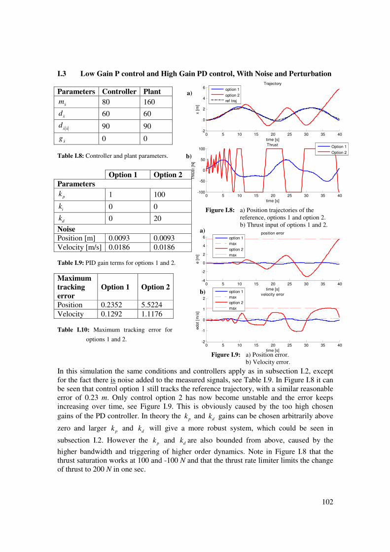
102


b) Velocity error.

I.3 Low Gain P control and High Gain PD control, With Noise and Perturbation




options 1 and 2.

In this simulation the same conditions and controllers apply as in subsection I.2, except

for the fact there is noise added to the measured signals, see Table I.9. In Figure I.8 it can

be seen that control option 1 still tracks the reference trajectory, with a similar reasonable

error of 0.23 m. Only control option 2 has now become unstable and the error keeps

increasing over time, see Figure I.9. This is obviously caused by the too high chosen

gains of the PD controller. In theory the pk and

dk gains can be chosen arbitrarily above

zero and larger p

k and dk will give a more robust system, which could be seen in

subsection I.2. However the pk and dk are also bounded from above, caused by the

higher bandwidth and triggering of higher order dynamics. Note in Figure I.8 that the

thrust saturation works at 100 and -100 N and that the thrust rate limiter limits the change

of thrust to 200 N in one sec.


xm& 80 160

xd & 60 60

x xd & &

90 90

xg & 0 0

Option 1 Option 2

Parameters

pk

1 100

ik 0 0

dk 0 20

Noise

Position [m] 0.0093 0.0093

Velocity [m/s] 0.0186 0.0186

Maximum

tracking

error

Option 1 Option 2

Position 0.2352 5.5224

Velocity 0.1292 1.1176




0 5 10 15 20 25 30 35 40-2

0

2

4

6

time [s]

x [

m]

Trajectory

option 1

option 2

ref traj

0 5 10 15 20 25 30 35 40-100

-50

0

50

100

time [s]

Thru

st

[N]

Thrust

Option 1

Option 2

0 5 10 15 20 25 30 35 40-4

-2

0

2

4

6

time [s]

e [

m]

position error

option 1

max

option 2

max

0 5 10 15 20 25 30 35 40-2

-1

0

1

2

time [s]

edot

[m/s

]

velocity error

option 1

max

option 2

max

a)

b)

a)

b)

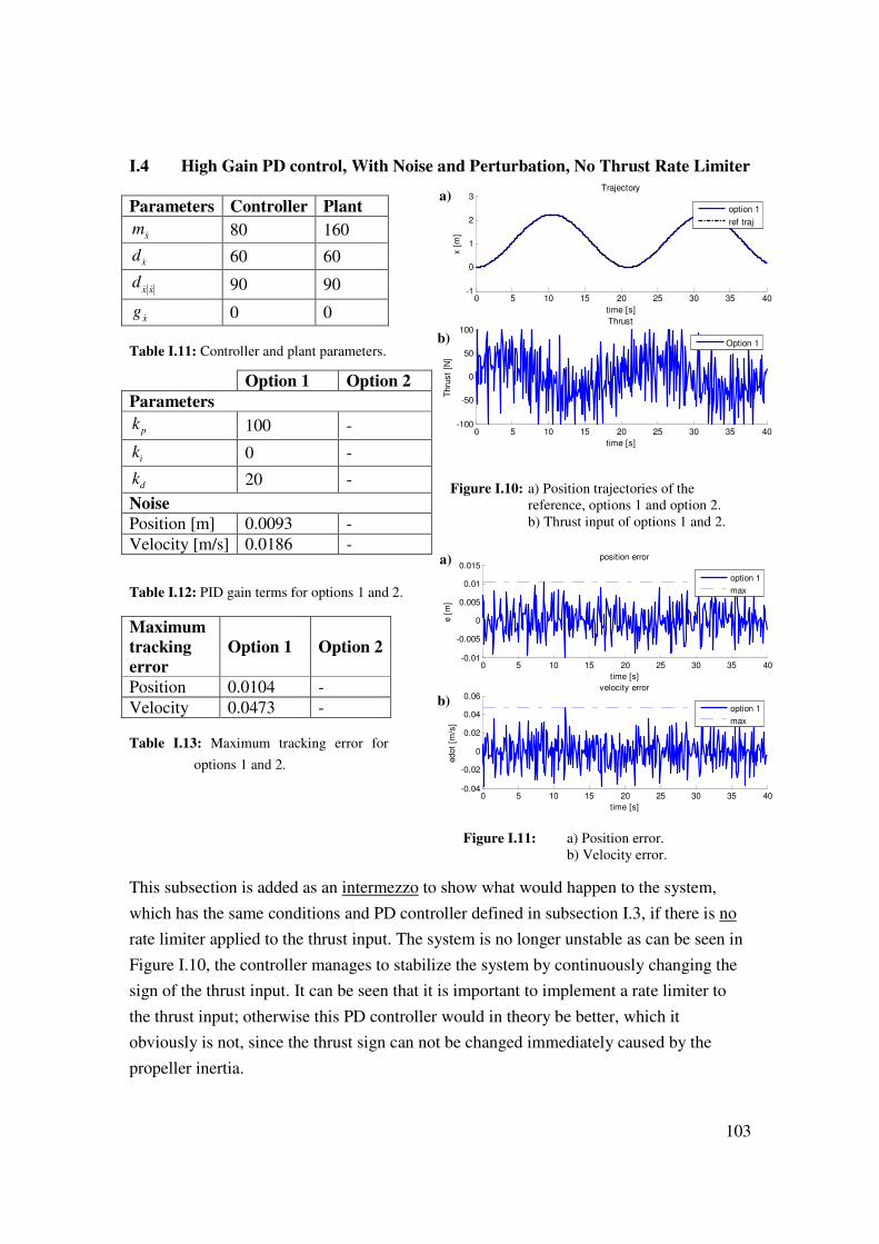
103

0 5 10 15 20 25 30 35 40-0.01

-0.005

0

0.005

0.01

0.015

time [s]

e [

m]

position error

option 1

max

0 5 10 15 20 25 30 35 40-0.04

-0.02

0

0.02

0.04

0.06

time [s]

edot

[m/s

]

velocity error

option 1

max

I.4 High Gain PD control, With Noise and Perturbation, No Thrust Rate Limiter




options 1 and 2.

This subsection is added as an intermezzo to show what would happen to the system,

which has the same conditions and PD controller defined in subsection I.3, if there is no

rate limiter applied to the thrust input. The system is no longer unstable as can be seen in

Figure I.10, the controller manages to stabilize the system by continuously changing the

sign of the thrust input. It can be seen that it is important to implement a rate limiter to

the thrust input; otherwise this PD controller would in theory be better, which it

obviously is not, since the thrust sign can not be changed immediately caused by the

propeller inertia.


xm& 80 160

xd & 60 60

x xd & &

90 90

xg & 0 0

Option 1 Option 2

Parameters

pk

100 -

ik 0 -

dk 20 -

Noise

Position [m] 0.0093 -

Velocity [m/s] 0.0186 -

Maximum

tracking

error

Option 1 Option 2

Position 0.0104 -

Velocity 0.0473 -


b) Velocity error.




0 5 10 15 20 25 30 35 40-1

0

1

2

3

time [s]

x [

m]

Trajectory

option 1

ref traj

0 5 10 15 20 25 30 35 40-100

-50

0

50

100

time [s]T

hru

st

[N]

Thrust

Option 1

a)

b)

a)

b)

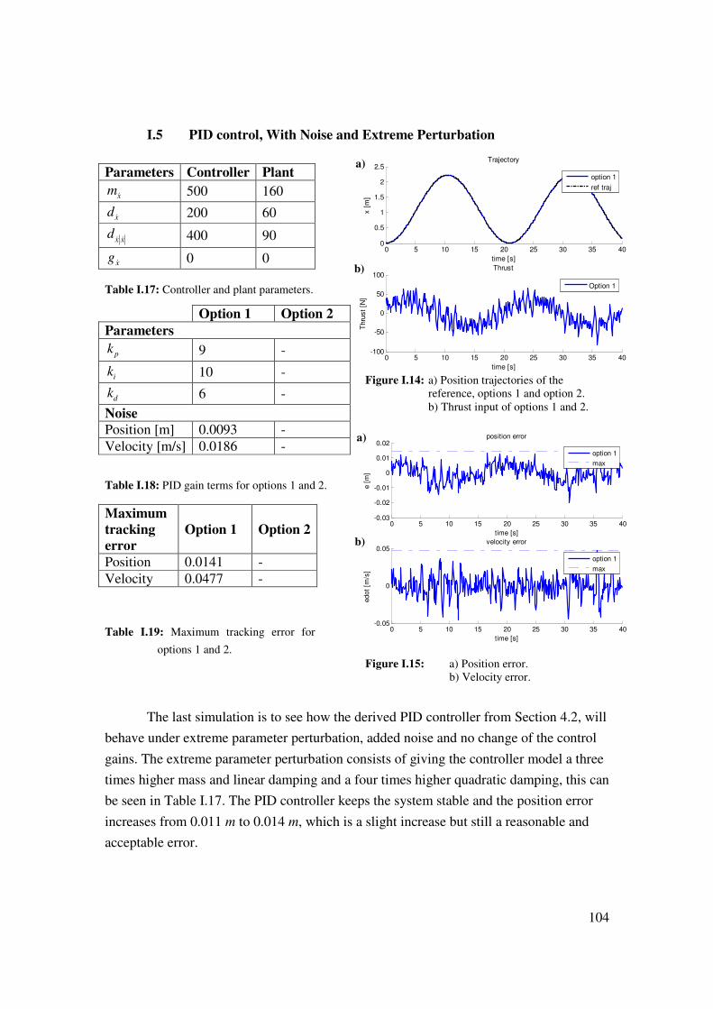
104

0 5 10 15 20 25 30 35 40-0.03

-0.02

-0.01

0

0.01

0.02

time [s]

e [

m]

position error

option 1

max

0 5 10 15 20 25 30 35 40-0.05

0

0.05

time [s]

edot

[m/s

]

velocity error

option 1

max

I.5 PID control, With Noise and Extreme Perturbation




options 1 and 2.

The last simulation is to see how the derived PID controller from Section 4.2, will

behave under extreme parameter perturbation, added noise and no change of the control

gains. The extreme parameter perturbation consists of giving the controller model a three

times higher mass and linear damping and a four times higher quadratic damping, this can

be seen in Table I.17. The PID controller keeps the system stable and the position error

increases from 0.011 m to 0.014 m, which is a slight increase but still a reasonable and

acceptable error.


xm& 500 160

xd & 200 60

x xd & &

400 90

xg & 0 0

Option 1 Option 2

Parameters

pk 9 -

ik 10 -

dk 6 -

Noise

Position [m] 0.0093 -

Velocity [m/s] 0.0186 -

Maximum

tracking

error

Option 1 Option 2

Position 0.0141 -

Velocity 0.0477 -


b) Velocity error.




0 5 10 15 20 25 30 35 400

0.5

1

1.5

2

2.5

time [s]

x [

m]

Trajectory

option 1

ref traj

0 5 10 15 20 25 30 35 40-100

-50

0

50

100

time [s]T

hru

st

[N]

Thrust

Option 1

a)

b)

a)

b)

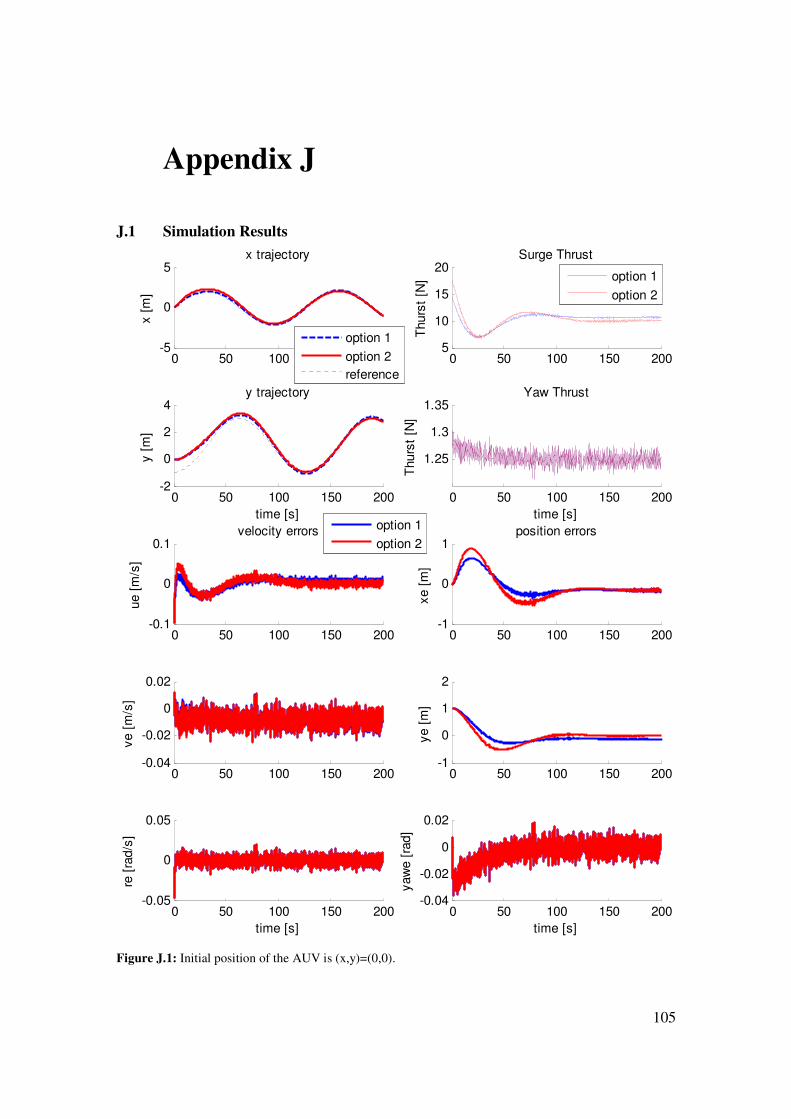
105

Appendix J

J.1 Simulation Results

0 50 100 150 200-5

0

5

x [

m]

x trajectory

option 1

option 2

reference

0 50 100 150 200-2

0

2

4

time [s]

y [

m]

y trajectory

0 50 100 150 2005

10

15

20

Thurs

t [N

]

Surge Thrust

option 1

option 2

0 50 100 150 200

1.25

1.3

1.35

time [s]

Thurs

t [N

]

Yaw Thrust

0 50 100 150 200-0.1

0

0.1

ue [

m/s

]

velocity errors

0 50 100 150 200-0.04

-0.02

0

0.02

ve [

m/s

]

0 50 100 150 200-0.05

0

0.05

time [s]

re [

rad/s

]

option 1

option 2

0 50 100 150 200-1

0

1

xe [

m]

position errors

0 50 100 150 200-1

0

1

2

ye [

m]

0 50 100 150 200-0.04

-0.02

0

0.02

time [s]

yaw

e [

rad]

Figure J.1: Initial position of the AUV is (x,y)=(0,0).

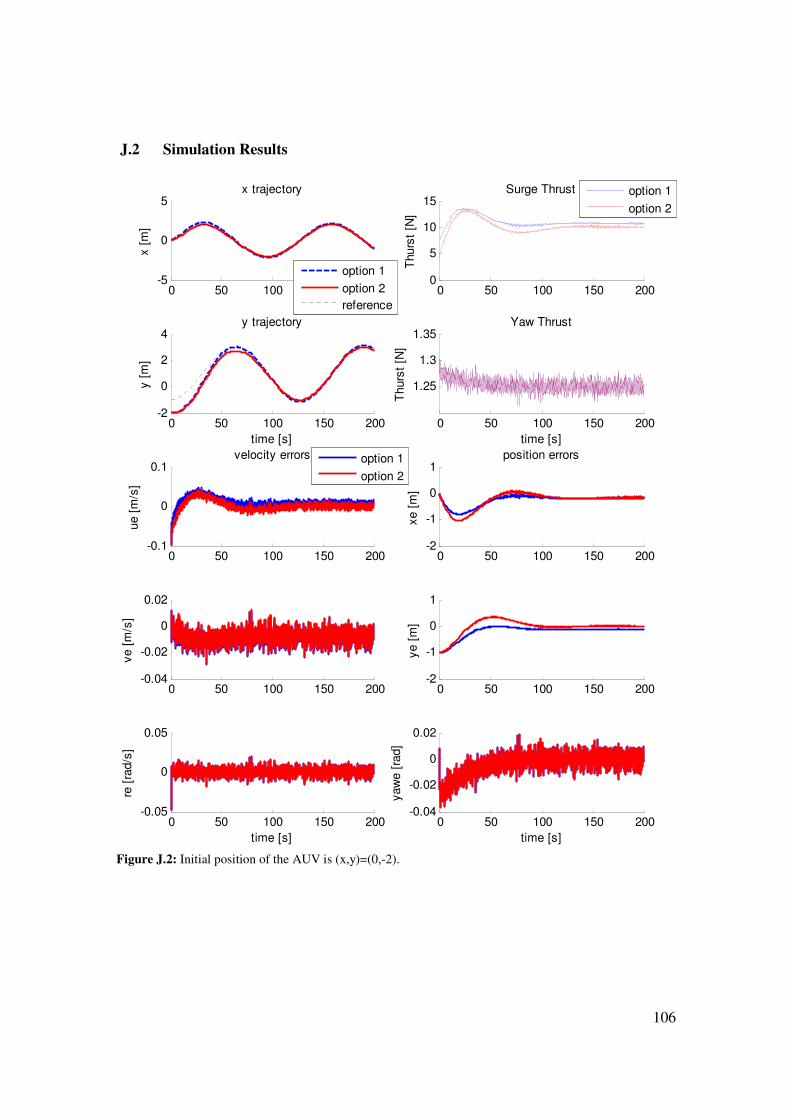
106

J.2 Simulation Results

0 50 100 150 200-5

0

5

x [

m]

x trajectory

option 1

option 2

reference

0 50 100 150 200-2

0

2

4

time [s]

y [

m]

y trajectory

0 50 100 150 2000

5

10

15

Thurs

t [N

]

Surge Thrust

option 1

option 2

0 50 100 150 200

1.25

1.3

1.35

time [s]

Thurs

t [N

]

Yaw Thrust

0 50 100 150 200-0.1

0

0.1

ue [

m/s

]

velocity errors

0 50 100 150 200-0.04

-0.02

0

0.02

ve [

m/s

]

0 50 100 150 200-0.05

0

0.05

time [s]

re [

rad/s

]

option 1

option 2

0 50 100 150 200-2

-1

0

1

xe [

m]

position errors

0 50 100 150 200-2

-1

0

1

ye [

m]

0 50 100 150 200-0.04

-0.02

0

0.02

time [s]

yaw

e [

rad]

Figure J.2: Initial position of the AUV is (x,y)=(0,-2).

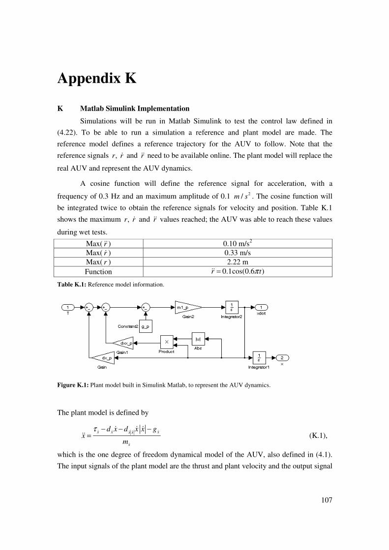
107

Appendix K

K Matlab Simulink Implementation

Simulations will be run in Matlab Simulink to test the control law defined in

(4.22). To be able to run a simulation a reference and plant model are made. The

reference model defines a reference trajectory for the AUV to follow. Note that the

reference signals , r r& and r&& need to be available online. The plant model will replace the

real AUV and represent the AUV dynamics.

A cosine function will define the reference signal for acceleration, with a

frequency of 0.3 Hz and an maximum amplitude of 0.1 2/m s . The cosine function will

be integrated twice to obtain the reference signals for velocity and position. Table K.1

shows the maximum , r r& and r&& values reached; the AUV was able to reach these values

during wet tests.

Max( r&&) 0.10 m/s2

Max( r& ) 0.33 m/s

Max( r ) 2.22 m

Function 0.1cos(0.6 )r tπ=&&

Table K.1: Reference model information.

Figure K.1: Plant model built in Simulink Matlab, to represent the AUV dynamics.

The plant model is defined by

x x xx x

x

d x d x x gx

m

τ − − −=

& & && &

&

& & &&& (K.1),

which is the one degree of freedom dynamical model of the AUV, also defined in (4.1).

The input signals of the plant model are the thrust and plant velocity and the output signal

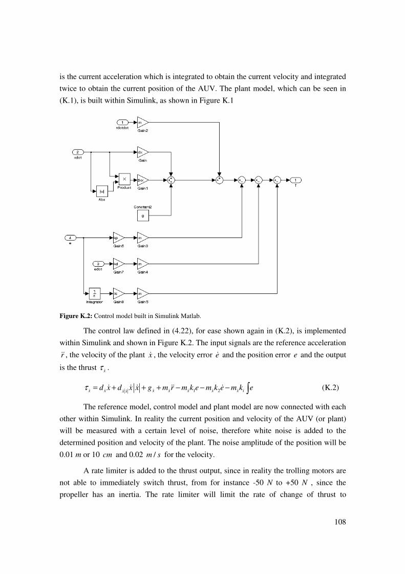
108

is the current acceleration which is integrated to obtain the current velocity and integrated

twice to obtain the current position of the AUV. The plant model, which can be seen in

(K.1), is built within Simulink, as shown in Figure K.1

Figure K.2: Control model built in Simulink Matlab.

The control law defined in (4.22), for ease shown again in (K.2), is implemented

within Simulink and shown in Figure K.2. The input signals are the reference acceleration

r&&, the velocity of the plant x& , the velocity error e& and the position error e and the output

is the thrust xτ & .

1 2x x x x x x x ix xd x d x x g m r m k e m k e m k eτ = + + + − − − ∫& & & & & & && &

& & & && & (K.2)

The reference model, control model and plant model are now connected with each

other within Simulink. In reality the current position and velocity of the AUV (or plant)

will be measured with a certain level of noise, therefore white noise is added to the

determined position and velocity of the plant. The noise amplitude of the position will be

0.01 m or 10 cm and 0.02 /m s for the velocity.

A rate limiter is added to the thrust output, since in reality the trolling motors are

not able to immediately switch thrust, from for instance -50 N to +50 N , since the

propeller has an inertia. The rate limiter will limit the rate of change of thrust to

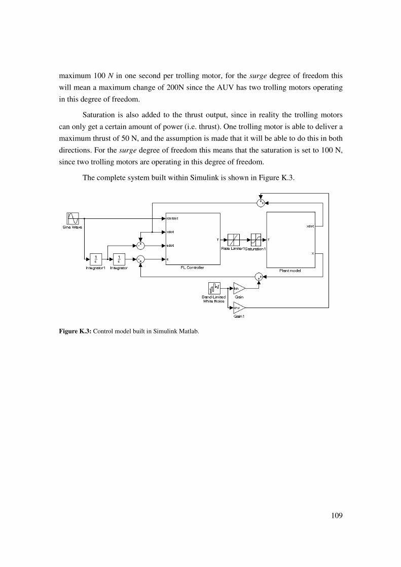
109

maximum 100 N in one second per trolling motor, for the surge degree of freedom this

will mean a maximum change of 200N since the AUV has two trolling motors operating

in this degree of freedom.

Saturation is also added to the thrust output, since in reality the trolling motors

can only get a certain amount of power (i.e. thrust). One trolling motor is able to deliver a

maximum thrust of 50 N, and the assumption is made that it will be able to do this in both

directions. For the surge degree of freedom this means that the saturation is set to 100 N,

since two trolling motors are operating in this degree of freedom.

The complete system built within Simulink is shown in Figure K.3.

Figure K.3: Control model built in Simulink Matlab.

Modeling and Control of an Unmanned Underwater · PDF fileModeling and Control of an Unmanned...

Documents

Transcript of Modeling and Control of an Unmanned Underwater · PDF fileModeling and Control of an Unmanned...