Modeling a healthcare system as a queueing network:The case of a Belgian hospital

Stefan Creemers and Marc R. Lambrecht

DEPARTMENT OF DECISION SCIENCES AND INFORMATION MANAGEMENT (KBI)

Faculty of Economics and Applied Economics

KBI 0710

Modeling a Healthcare System as a Queueing Network: The Case of a

Belgian Hospital

Stefan CREEMERS and Marc R. LAMBRECHT

Department of Decision Sciences & Information Management,Research Center for Operations Management,

Katholieke Universiteit Leuven,Naamsestraat 69, 3000 Leuven, Belgium.

ABSTRACT

The performance of healthcare systems in terms of patient flow times and utilization of critical

resources can be assessed through queueing and simulation models. We model the orthopaedic

department of the Middelheim hospital (Antwerpen, Belgium) focusing on the impact of outages

(preemptive and nonpreemptive outages) on the effective utilization of resources and on the flow

time of patients. Several queueing network solution procedures are developed such as the decom-

position and Brownian motion approaches. Simulation is used as a validation tool. We present new

approaches to model outages. The model offers a valuable tool to study the trade-off between the

capacity structure, sources of variability and patient flow times.

Topic areas: health care, performance measurement, capacity management

Methodological areas: queueing theory, stochastic processes, case studies

1

INTRODUCTION

In this paper we present a case study of the Middelheim hospital (Antwerpen, Belgium) in which

we analyze performance (in terms of total patient waiting times or flow times) of the orthopaedic

department. For this purpose we construct an open queueing network using a decomposition ap-

proach (Lambrecht, Ivens, & Vandaele, 1998) as well as a Brownian queueing model (Harrison,

1988). Both models are compared and validated using a simulation study. In addition we assume

preemptive and nonpreemptive outages to take place and develop exact and approximate closed

form expressions to assess their impact on patient flow times.

Economies around the world are more and more focussed on service industries in general and

healthcare in particular (Bretthauer, 2004; Zhu, Sivakumar, and Parasuraman, 2004). In addition,

patient flow times play an increasingly important role in today’s healthcare systems. Government

reimbursement systems (based on a justified length of stay), insurer’s rejection of reimbursement

(i.e. denied days), competition between hospitals, government regulations and patient satisfaction

urge hospital decision makers to find ways to decrease waiting times (both waiting time inside the

hospital as well as the waiting list that exists outside the hospital). Current healthcare literature and

practice indicate that waiting lists and congested patient flows do indeed make up for one of the

most important problems in care industries (Worthington, 1987 and 1991; Cerda, de Pablos, & Ro-

driguez, 2006; Belson, 2006). In order to improve performance in an environment as complex as

a hospital system, the dynamics at work need to be understood. To obtain such an understanding,

queueing theory and simulation provide an ideal set of tools. Healthcare systems however have a

number of specific features as compared to manufacturing systems, posing important methodolog-

ical challenges.

With respect to queueing theory, a historic overview may be found with Stidham (2002) and

Green (2006). In healthcare, queueing theory has been used to assess capacity requirements (Kao

& Tung, 1981; Worthington, 1987; Green, 2003; McManus, Long, Cooper, & Litvak, 2004), out-

patient scheduling (Cayirli & Veral, 2003), process optimization (Vandaele, Van Nieuwenhuyse,

& Cupers, 2003b) and absence recovery modeling (Easton & Goodale, 2005). The greater part

2

of literature is dedicated to single station queueing systems. Queueing networks are only scarcely

dealt with (Koizumi, Kuno, & Smith, 2005). Simulation on the other hand is much more prevalent.

An extensive overview of the use of discrete event simulation in healthcare research can be found

in Jacobson, Hall, and Swisher (2006).

With respect to service outages and server unreliability, a large body of literature is available.

A survey on literature on the machine interference problem can be found in Stecke and Aronson

(1985) and Haque and Armstrong (2007). Unreliable servers are often modeled using vacation

models in which a system alternates between periods when a service is available (on-periods) and

periods when the service is unavailable (off-periods) (Federgruen and Green, 1986). An alternative

approach is suggested in Hopp and Spearman (2000). In their work Hopp et al. (2000) propose a

transformation of the service process times to account for service outages. In what follows we pro-

vide an extension of this procedure. Outages in a hospital setting have been studied by Babes and

Sarma (1991), Liu and Liu (1998a), Chisholm, Collison, Nelson, and Cordell (2000), Chisholm,

Dornfeld, Nelson, and Cordell (2001), France, Levin, Hemphill, Chen, Rickard, Makowski, Jones,

and Aronsky (2005) and Gabow, Karkhanis, Knight, Dixon, Eiser, and Albert (2006) among others.

The remainder of this article is structured as follows: in an upcoming section, we describe

the problem setting. Next we delve deeper into the queueing methodology required to tackle

the problem at hand; we discuss the queueing model using a parametric decomposition approach

and also introduce a Brownian queueing model. This is followed by a section dedicated to the

simulation model and a section that focusses on the testing of different scenarios in which the

impact of outages is gradually decreased. A last section presents the conclusions.

PROBLEM DESCRIPTION

The case-study which is the subject of this paper deals with the Middelheim hospital in Antwerpen,

Belgium. With a capacity of more than 600 beds it can be considered as one of the largest care

institutions of the country. In addition the Middelheim hospital is the largest member of a hospital

3

Figure 1: Capacity structure of the orthopaedic department of the Middelheim hospital

network accounting for a total yearly number of 75,000 hospitalizations. While the detailed study

of such a system in its entirety is virtually impossible, we decided to confine ourselves to the

analysis of the orthopaedic department at the Middelheim hospital. The orthopaedic department

currently has six surgeons and can rely on a medical staff of over 15 nurses. On a yearly basis

3,300 patients are being operated and more than 13,000 patients receive consult. Typically the

department consists of three workcentres: consultation, surgery and recovery. With respect to

orthopaedics, three consultation rooms are available. For purposes of surgery, the department

has exclusive access to one operating theatre and claims half the capacity of two other theatres

(resulting in the capacity-equivalent of two operating theatres). The process of recovery takes

place in an internal or external ward or in the day hospital. In each of these wards a capacity of

25 beds is reserved for the orthopaedic patients. The capacity structure is illustrated in Figure 1.

Obviously some of these workstations (i.e. consultation and surgery) do not operate continously,

but rather during predefined time intervals. As such these workstations are unavailable for service

at certain moments in time. In order to determine the availability of a workstation one needs to

observe the work schedules of surgeons and medical staff that operate the orthopaedic department.

In addition, deviations from these work schedules (as a result of overtime, holidays, . . . ) need to

be taken into account.

4

Due to the high level of heterogeneity between patients, we need a grouping mechanism in

order to construct a workable model. The use of Diagnosis Related Groups (DRGs) arises naturally

(Roth & Van Dierdonck, 1995; van Merode, Groothuis, & Hasman, 2004). In healthcare DRGs

are used to define groups of patients who have a similar treatment process and who consume

comparable amounts of resources (Fetter, 1991). Mostly a DRG is constructed around a specific

pathology (e.g. APR-DRG 302; major surgery on joints and the reattachment of lower limbs) and

holds the information concerning how this pathology should be treated and which resources should

be addressed in doing so. As such they are important decisions tools for hospital management and

governments. In fact, more and more governments have the tendency to reimburse hospitals by

taking into consideration the Length of Stay (LoS; the interval between the surgery date and the

discharge from the hospital) of a patient belonging to a certain DRG (Cots, Elvira, Castells, &

Dalmau, 2000; Sutherland & Botz, 2006). For example, with respect to APR-DRG 302, a Belgian

hospital receives a fee corresponding to a patient sojourn ranging from a minimum of 14 days up

to a maximum of 55 days (the actual compensation depends on the severity of illness and the age

of the patient since both parameters exert great influence on patient LoS). This duration is also

referred to as the Justified LoS or JLoS for those patients belonging to APR-DRG 302. If the

patient in question is dismissed after a mere seven days, the hospital still collects the total amount

of the fee. On the other hand, if the patient remains in care for a period which exceeds the limit of

the JLoS, the hospital has to pay for the additional costs by themselves. Moreover the JLoS of a

certain DRG is determined in function of the national average LoS of that DRG and is updated on a

yearly basis. As such, the system stimulates hospitals to continuously improve their performance.

This argument is one of the most important drivers for the study reported in this paper.

Previously we have already hinted at the diversity of our patient population and the need to

create some structure therein. Using the DRG classification of patients as a working basis, we

were able to extract 18 homogenous patient classes (most of them containing only a select set of

DRGs). Each of these patient classes corresponds to a unique set of routings, service and arrival

rates and resources required at each step of the treatment process. These data have been acquired

5

Figure 2: Patient flow at the orthopaedic department of the Middelheim hospital

through means of existing databases, field studies and expert information. In total the records

of 3,294 patients were selected for further study. Throughout the text, we will use these data to

numerically illustrate the model. The detailed manipulation of the data will not be given.

In a nutshell, the treatment process of any patient (belonging to one of the 18 classes) at the

orthopaedic department starts with one or more consultations followed by surgery, recovery and a

number of follow-up consultations. We assume that every patient receives at least one consultation

before as well as after surgery. After completion of the follow-up consultations the patient leaves

the hospital. As a consequence, re-entry of patients is only possible at the consultation level while

other workstations are visited exactly once. A general outline of the model can be found with

Figure 2.

To further enhance the understanding of the model we provide a timeline of one particular

pathology group. For instance observe those patients who suffer from the Carpal Tunnel Syn-

drome (CTS). In the model this group of patients is comprised within class 12 while on the level

of DRGs they can be categorized as APR-DRG 025. The empirical data shows that on average

216 of these patients arrive at the Middelheim hospital each year. Hence the external arrival rate

of CTS-patients equals 0.59 patients per day. In our model an external arrival refers to the making

6

of a first appointment. Upon arrival (i.e. after an appointment is made) the patient enters the queue

and waits until a consultation time slot becomes available. The waiting process of a patient can

be divided in two distinct phases (Vissers, Bertrand, & De Vries, 2001; Hall, Belson, Muralli, &

Dessouky, 2006); the time spent waiting inside and outside the hospital. The former being defined

as the internal waiting time (i.e. the time spent waiting in the hospital before treatment) while the

latter consists of the waiting list and a certain amount of time spent waiting prior to making an ap-

pointment. The time spent waiting between service completion and the making of an appointment

can often be assigned to personal reasons or to reasons associated with the treatment process itself

(for instance, patients who have their hip replaced face two-yearly follow-up consultations). While

patients do not experience this time interval as time spent waiting prior to treatment, it cannot be

considered as a key element contributing to patient flow times. Therefore we do not take into ac-

count the time spent waiting between service completion and the making of an appointment. As

such we confine ourselves to the study of the waiting list and the time spent in the hospital. To-

gether with the processing time, both forms of waiting combined constitute the total waiting time

(throughout this paper, we will use the terms total waiting time and flow time interchangeably).

Typical to most patient classes and hospital environments, the waiting list substantially exceeds the

internal waiting time.

The duration of the consultation itself is drawn from an empirically established distribution.

After a first consultation two routing options arise; there exists a probability that the patient di-

rectly advances towards the next workcentre (surgery) or alternatively the patient might require

some additional consultations before enduring surgery (i.e. the patient re-enters at the consultation

queue). In general CTS-patients undergo 2.3 consultations before being directed towards surgery.

Once arrived at the second workstation, patients are once more introduced into a queue and are held

there until they can be fit into the surgery planning schedule. After surgery, the patient is trans-

ferred to the day hospital or one of the two recovery wards. It is important to note that, despite the

limited capacity of the nursing units, surgeries will never be postponed due to the shortage of bed

capacity at the wards. In the occasion that such a shortage occurs, a solution is found in dialogue

7

Figure 3: Sample treatment path of a CTS-patient

with the other hospital departments (i.e. the patient will recover at another department which has

excess capacity). After the revalidation has been completed, the patient is discharged from the hos-

pital and is subjected to a number of follow-up consultations. In other words, the patient re-enters

the consultation queue. On average patients suffering from CTS endure 1.13 follow-up consulta-

tions after which they are dismissed from the hospital as well as from the model. A visualization

of the treatment process of an exemplary CTS-patient is given in Figure 3.

Another important determinant of the flow time is variability (Hopp et al., 2000). Within vari-

ability we make a distinction between variability that can be assigned a cause (i.e. assignable-cause

variability) and variability that is inherent to the system processes (i.e. natural variability). Regret-

tably, in comparison with manufacturing environments, natural variability is much more substantial

in services industry in general and in healthcare in particular (McLaughlin, 1996; Tsikriktsis and

Heineke, 2004). For instance, it requires only little imagination to grasp the difference between

the assembly of a car and the treatment process of a patient. As for assignable-cause variability

one can once more distinguish between the variability originating from causes one can control and

conversely the variability created by causes which remain beyond our direct control. Examples

of the latter category include the patient arrival pattern as well as the diversity of the patient mix

(although it could be argued that even the patient mix is controllable to some degree; by denying

access to certain types of patients or by making investments in order to accommodate for certain

patient groups). All types of variability have an impact on flow times. The greater part of litera-

ture focusses mainly on variability resulting from patient behavior (e.g. the arrival of unscheduled

patients, patients that fail to show up, . . . ). In this paper however, we focus on unplanned absences

8

of medical staff and interruptions during service operations. Unplanned absences and interrup-

tions during service activities have a major impact on flow times. Doctors and medical staff face

various obligations which they have to attend to (making morning rounds, answering phones, pa-

tient check-ups, daily management, . . . ). In addition doctors often combine a hospital job and

private consultation. These phenomena may cause a variable arrival pattern at the hospital (Liu

et al., 1998a) and may lead to interruptions during the treatment process (Chisholm et al., 2000;

Chisholm et al., 2001; Easton et al., 2005; Gabow et al., 2006). It is clear that hospital environ-

ments are characterized by substantial amounts of variability. As is argued in literature (Hopp

et al., 2000), variability induces waiting times. While in services industries variability cannot be

countered by means of inventory in the traditional sense, patients will have to wait until capacity

becomes available (Vissers et al., 2001; Harper, 2002; Vandaele & De Boeck, 2003a; Sethuraman

& Tirupati, 2005). Besides the time buffer, hospitals often have to rely on a capacity buffer to

mitigate the impact of variability and to maintain required service levels.

The above problem description illustrates the complexity of modeling healthcare systems.

More importantly, the specific features described above (re-entry of patients, stochastic routings,

time blocks for consultation and surgery, absences and interruptions, service time variability, . . . )

pose important methodological challenges. These issues are the subject of the next section.

MODELING THE HEALTHCARE SYSTEM AS A QUEUEING MODEL

In this section we develop the queueing models of the orthopaedic department at the Middelheim

hospital. The models will be validated through simulation. We suggest two approaches:

• Parametric decomposition; using the Kingman equation (Hopp et al., 2000) and the approx-

imation derived by Whitt (1993) to assess performance.

• A Brownian queueing model (Harrison, 1988; Chen, Shen, & Yao, 2002).

These two approaches are discussed in the upcoming sections.

9

Figure 4: Queueing network blueprint of the orthopaedic department at the Middelheim hospital

Parametric Decomposition

In this section we discuss the parametric decomposition approach initiated by Jackson (1957). First

we provide a model description and define the primitive processes. Next we adapt the model to

include the effects of preemptive and nonpreemptive outages. Finally, arrival and service processes

are aggregated and a number of flow time expressions are surveyed.

Modeling arrival rate and natural service times

The queueing network representation of the orthopaedic department is given in Figure 4. The

queueing model represents an open re-entry network that consists of five G/G/m workcentres (con-

sultation, surgery and three wards representing the locations at which recovery takes place). The

queueing network is modeled using the principles of the decomposition technique that was pi-

oneered by Jackson (1957 and 1963) and further refined by authors such as Shanthikumar and

Buzacott (1981), Bitran and Tirupati (1988), Lambrecht et al. (1998) and Vandaele, De Boeck,

10

and Callewier (2002). The queue discipline adhered at each of the stations is FCFS. Any variation

in the arrival of patients (e.g. the early, late, unannounced or not showing up of patients) is pre-

sumed to be absorbed in the variance of the arrival process. The model assumes infinite buffers

to exist in front of every queue. Realizing that the buffers in front of the consultation and surgery

workstation correspond to their respective waiting lists, it would be incorrect to restrain them in

size. In real life, if patients contact the hospital to make an appointment for a consultation or a

surgery, they will be issued an appointment date no matter how far ahead in time this date might be

(i.e. we assume patients not to display any balking- or reneging-behavior when arriving or abiding

at the queue). Hence buffer capacities are virtually unlimited. With respect to the recovery wards,

one might argue that queue capacity is in fact limited. However, there are several reasons that are

able to question this assertion. Next to rendering the model highly intractable, finite buffers do

not necessarily correspond to reality since shortages of bed capacity at the wards are solved at the

local level and in general do not prolong the sojourn time of a patient (this of course presumes

the presence of unoccupied beds somewhere in the hospital). Therefore we will assume infinite

buffers at all stages of the treatment process. Considering the multiclass re-entry environment of

the queueing network, aggregation of the arrival and service process is required in order to perform

a decomposition-based queueing analysis.

More formally, let i denote the workstation in the network; i ∈ {1, . . . , I}. Each workstation

i operates mi parallel servers (for instance, at consultation three patients can be processed simul-

taneously). Have station 1 to 5 represent consultation, surgery, day hospital, internal ward and

external ward respectively. Let k stand for the patient class; k ∈ {1, . . . , K}. Hence we have K

classes of patients visiting a set of I workstations. Patients belonging to different classes are al-

lowed to differ in terms of interarrival times, service times and routing. Assume interarrival times

and service times of patients to be i.i.d. if they belong to one and the same class and assume them to

be independently (but not necessarily identically) distributed otherwise. Let ηk denote the external

arrival rate of class k patients at the consultation workstation (i.e. the only station at which external

11

arrivals are assumed to take place). The aggregate external arrival rate at consultation equals:

η =K∑k=1

ηk (1)

We assume that the time intervals between the external arrivals are exponentially distributed. Such

an assumption poses only a slight restriction on the accuracy of the model while it has been shown

by Palm (1943) and Khinchin (1960) that the sum of a large numbers of independent renewal

processes (i.e. the arrival processes of the different classes of patients) will tend to a Poisson

process. Considering the multitude of classes of patients, the approximation of the aggregate

external arrival process by means of a Poisson process should be accurate. Next let γk denote the

expected number of visits a class k patient will pay to the first workstation. The aggregate arrival

rate of patients at consultation equals:

λ1 =K∑k=1

ηkγk (2)

Remark that in contrast to the aggregate external arrival rate, which was assumed to be Poisson-

distributed, the aggregate arrival rate (at each of the workstations) is allowed to follow a general

distribution. Further define the routing matrix R in which the elements rij indicate the probability

of a patient to travel from station i to station j after service completion at station i. Adhering to

standard conventions, we establish a node (of index i = 0) from which external arrivals originate

and which also serves as a sink for patients leaving the hospital system. Let ri0 indicate the prob-

ability of leaving the system when departing from station i. Conversely r0i implies the probability

of an external arrival occurring at station i. The probabilities rij can be expressed as the the pro-

portion of the arrivals at station i that travel towards station j. When assuming the stability of the

queueing network, the law of conservation of flows dictates:

r10 =η

λ1

(3)

12

While each patient visiting the orthopaedic department is subjected to surgery exactly once, one

can infer that (λ2 = η). Hence the probability of transition from the consultation to the surgery

level equals:

r12 =η

λ1

(4)

Considering the fact that transitions towards recovery are impossible we have that:

r11 = 1− (r10 + r12) = 1− 2η

λ1

(5)

With respect to the recovery workstations we have access to empirically established arrival rates

from each of the observed patients (more specifically, we have knowledge of the location as well

as the duration of recovery from each of the 3,294 patients who endured surgery). As a result we

can obtain the routing probabilities as follows:

r2i =K∑k=1

λikλ2

∀i ∈ {3, 4, 5} (6)

Where λik is the observed arrival rate of class k patients at workstation i. It follows that:

λi =K∑k=1

λik ∀i ∈ {3, 4, 5} (7)

As such we have defined all of the routing probabilities that require computational effort. All other

routing probabilities stem directly from the structure of the model (e.g. the probability of returning

to the consultation workstation after the completion of recovery equals unity). The subsequent set

13

R =

i/j 0 1 2 3 4 5

0 0.00000 1.00000 0.00000 0.00000 0.00000 0.00000

1 0.24687 0.50627 0.24687 0.00000 0.00000 0.00000

2 0.00000 0.00000 0.00000 0.51350 0.41671 0.06978

3 0.00000 1.00000 0.00000 0.00000 0.00000 0.00000

4 0.00000 1.00000 0.00000 0.00000 0.00000 0.00000

5 0.00000 1.00000 0.00000 0.00000 0.00000 0.00000

Table 1: Transition matrix of the queueing model

of expressions completely defines the routing probabilities:

r1j = ηλiδ1j ∀j ∈ {0, 2, 3, 4, 5} ,

r11 = 1− 2ηλ1,

r2j = λjλ2δ2j ∀j ∈ {0, 1, 2, 3, 4, 5} ,

rij = δij ∀i ∈ {0, 3, 4, 5} ;∀j ∈ {0, 1, 2, 3, 4, 5} .

(8)

Where (δij = 1) if at least one of the patient classes travels from station i to station j and (δij = 0)

otherwise. The routing matrix R is presented in Table 1 (due to rounding some rows may not

add up to one). The numerical values recorded in Table 1 serve an illustrative purpose while paper

limitations do not accommodate for the treatment of detailed calculations. The routing probabilities

allow us to compute the aggregate arrival rates, which are presented in summary Table 2 at the end

of the section.

With respect to the service times, let fik (x) denote the natural service time probability density

function of a class k patient visiting workstation i. Have 1/νik and σ2νik

represent the average

natural service time for a class k patient at workstation i and its variance respectively. The natural

process time excludes random interruptions, absences and any other external influence. Assume

service times of different classes to be independent but not necessarily identically distributed. The

probability that a randomly picked unit in front of the workstation is of class k is given by λik/λi;

14

where λi is the total arrival rate at workstation i. Define the probability function of the aggregate

natural service times at station i as follows:

fi (x) =K∑k=1

λikλifik (x) (9)

As a result the average natural service time requirement of a unit in front of the workstation

amounts to:1

νi=

K∑k=1

λikλi

1

νik(10)

When observing the variance of the aggregate natural service process, one can deduce that its

formula boils down to:

σ2νi

=K∑k=1

λikλi

ˆ (x− 1

νi

)2

fik (x) dx (11)

This can be simplified to:

σ2νi

= − 1

ν2i

+K∑k=1

λikλi

(σ2νik

+1

ν2ik

)(12)

We refer to σ2νi

as a measure of the natural variability of the aggregate process times at workstation

i. The same result was obtained by Whitt (1983) and has widely been adopted in literature (Whitt,

1999; Haskose, Kingsman, & Worthington, 2002).

Variability from preemptive and nonpreemptive outages

As was indicated previously, the service process of a patient may be interrupted or postponed.

These outages will increase the natural service times. We call these increased, adjusted service

times, effective process service times. It is the total time ”seen” or ”experienced” by a patient at a

workstation. The effective process time random variable is of primary interest to determine flow

times.

We make a distinction between preemptive and nonpreemptive outages and assume them to

occur only at the consultation level. Preemptive and nonpreemptive outages will impact the service

process and will give rise to increased levels of traffic intensity (resulting in the so-called effective

15

utilization rate or effective traffic intensity).

Let us first discuss the nonpreemptive outages. Nonpreemptive outages typically occur between

jobs, rather than during jobs. They occur at the beginning of each service epoch (i.e. at the start of

a consultation work shift) whenever a doctor or another member of the medical staff is absent (e.g.

due to late arrival). We may refer to such an outage as unplanned absences and define the mean

and variance of the amount of time absent as 1/µs and σ2s respectively (i.e. general absence times

are presumed). Furthermore we assume an average number of patients (represented by n) to arrive

in between two consecutive absences. This is an important feature of the model. Indeed, n may

be considered as the number of patients in a consultation time block. Each start of a consultation

time block may induce a delay due to an absence. In other words, the number of patients in a

consultation time block is a decision variable and is comparable to a lot sizing decision. Evaluating

different time block sizes (i.e. different values of n) may provide key managerial insights.

Next to nonpreemptive outages, we also allow for preemptive outages to take place. Preemptive

outages occur whenever a doctor is interrupted during a consultation activity. These interruptions

will be modeled in an approach which builds on the tradition set by Hopp et al. (2000). They

are characterized by a Mean Time To Interrupt (τi) and a Mean Time To Resolve (τr). The model

presented in Hopp et al. (2000) presumes interrupts to occur only during actual service time.

However, in a hospital setting it is not inconceivable that interrupts take place during the resolve

time induced by a previous interrupt as well. For instance, if the service process of a patient is

interrupted by a phone call, it is still possible for a doctor to be called away for an emergency, to

receive another call, . . . .

In the upcoming sections expressions are developed to assess the impact of outages on mean

and variance of service times. In the computation of the effects of outages themselves, triangular

distributions of outage times (i.e. absence times as well as interrupt resolve times) were assumed.

The choice for a triangular distribution arises naturally while it proves convenient for field pro-

fessionals to provide minimum, maximum and mean estimates of absence and interruption times.

Including the impact of outages results in effective service times. These effective service times

16

will result in congestion, unstable schedules and most important in overtime for staff members.

We refer to Easton et al. (2005) for an excellent treatment of this issue.

Nonpreemptive outages

We define a nonpreemptive outage to occur whenever the succession of two events is based on the

number of services performed in between (hence, setups, rework, maintenance, . . . are all exten-

sions that are able to capitalize on the technique discussed in this section). Applied to our setting,

we have that n patients are treated (on average) in between two consecutive absence possibilities.

Assume that the length of services and absence times do not depend on the service history (i.e.

they are independent of prior services and absence times). The absence times themselves are dis-

tributed following a probability density function fs (x). The average absence time and its variance

are represented by 1/µs and σ2s . The service time of the nth patient includes part service time, part

absent time. We refer to the service time of the nth patient as the combined service time. The

probability density function of the combined service times equals:

fc (x+ y) =K∑k=1

λ1k

λ1

f1k (x) fs (y) (13)

One can view the services that are preceded by an absent period as a separate class of patients that

has a probability 1/n of randomly being picked in front of the workstation. The other services as a

whole have a probability ((n−1)/n) of randomly being picked. Therefore, we can define the mean

aggregate service times including the effect of absence times as follows: :

1

υ=

[(n− 1

n

) K∑k=1

λ1k

λ1

ˆf1k (x)xdx

]+

[1

n

K∑k=1

λ1k

λ1

¨f1k (x) fs (y) (x+ y) dydx

](14)

This can be simplified to:1

υ=

1

ν1

+1

nµs(15)

17

With respect to the variance of the aggregate service time (including absence times) at the consul-

tation workstation we develop the following expression:

σ2υ =

[(n−1n

) K∑k=1

λ1k

λ1

´f1k (x)

(x− 1

υ

)2dx

]+[

1n

K∑k=1

λ1k

λ1

˜f1k (x) fs (y)

(x+ y − 1

υ

)2dydx

] (16)

Further simplification yields:

σ2υ =

[σ2ν1

+(

1ν1− 1

υ

)2]

+[

1n

(σ2s + 1

µ2s

+ 2ν1µs

− 2υµs

)]= σ2

ν1+ σ2

s

n+ 1

µ2s

(n−1n2

) (17)

The above expression is equivalent to that of Hopp et al. (2000) and is valid under the assumption

that the combined service times as well as ordinary service times are independently distributed.

Preemptive outages

We refer to service interruptions as preemptive outages. Doctors being called away on emergen-

cies, answering phone calls, . . . are typical examples. The average time between two consecutive

interrupts is defined as τi whereas τr refers to the average time it takes to resolve an interruption.

Preemptive outages prove to be more difficult to model while they occur after the elapsing of a

variable amount of time (i.e. a mean time to interrupt; τi), rather than after a number of patients

being processed. Therefore patients characterized by a larger service time requirement are more

susceptible to preemptive outages; the probability of a preemptive outage occurring during the

processing of a patient depends on the length of service of that patient as well as on the length

of service of previous patients (i.e. the service history). Such dependencies tend to drastically

increase the complexity of the problem. Consequently the exact analysis often remains beyond

reach. Regarding our problem, we will show that expressions for the mean service time incorpo-

rating the impact of interrupts are easily obtained. Unfortunately, when assessing the variance of

the service times (including the effect of preemptive outages), we have to rely on approximations.

18

With respect to preemptive outages, we make a distinction between two different scenarios. On

the one hand, one might presume preemptive outages to occur only during actual service time; as

such preemptive outages do not take place during the resolve times induced by previous outages.

Remark that this does not imply that the service process of a single patient cannot be interrupted

more than once. On the other hand, one might assume preemptive outages to occur during resolve

times as well (e.g. as indicated previously, doctors may be be interrupted when already engaged in

resolving a previous interrupt). While this latter instance can be seen as an extension of the former,

we will first discuss outages occurring exclusively during actual service time. Define τr0j as the

resolve time of the jth preemptive outage that occurred during the service process of one and the

same patient. The mean and variance of the resolve times are given by τr and σ2r . In addition,

resolve times of different outages are assumed to be i.i.d.. The service process of a patient thus

faces the probability of encompassing several interrupts that prolong its service duration. The

service time of a patient (including interrupts) can be expressed as:

1

ω=

1

ν1

+J0∑j=1

τr0j (18)

As such, the average service time 1/ω incorporates both the natural service time 1/ν1 as well as

the resolve times of interrupts that occurred during service. Moreover, J0 denotes the number of

preemptive outages that occurred during the service process of a unit. J0 is a random variable that

follows a Poisson distribution (i.e. we assume the time between two consecutive interrupts to be

exponentially distributed). Hence its mean and variance both equal (1/(ν1τi)). We face a sum of

random variables (the resolve times; τr0j ) in which the number of random variables (the number of

interrupts; J0), is a random variable itself. Assume that J0 and τr0j (∀j ∈ N) are i.i.d. variables.

In addition assume the mean as well as the variance of τr0j to be equal for all j ∈ N. Therefore,

the mean and variance of the sum of J0 random variables τr0j can be expressed as (Dudewicz &

Mishra, 1988):

E [S0] = E [J0]E[τr0j

](19)

19

σ2S0

= E [J0]σ2r + E

[τr0j

]2σ2J0

(20)

Where S0 is the random variable representing the sum of J0 resolve times τr0j . In other words we

have that:

S0 =J0∑j=1

τr0j (21)

The mean and variance of the sum of resolve times can be defined as:

E [S0] =1

ν1

τrτi

(22)

σ2S0

=1

ν1

σ2r + τ 2

r

τi(23)

We can now express the mean aggregate service time including the effect of interrupts as follows:

E[

1ω

]= Eν1

[EJ0

[1ω

]]= Eν1

[EJ0

[1ν1

+J0∑j=1

τr0j

]]

= Eν1[EJ0

[1ν1

+ S0

]]= Eν1

[1ν1

+ τrν1τi

]= Eν1

[τi+τrν1τr

]= τi+τr

ν1τi

= 1ν1

τi+τrτi

(24)

This corresponds to the expression presented in Hopp et al. (2000) in which the natural service

time is divided by an availability factor in order to incorporate the effect of interrupts. Next we

have a look at the variance of the service times including the effect of preemptive outages during

20

service time. We start with the approximation of the second moment:

E[(

1ω

)2]

= Eν1

[EJ0

[(1ω

)2]]

= Eν1

EJ0

( 1ν1

+J0∑j=1

τr0j

)2

= Eν1

[EJ0

[(1ν1

+ S0

)2]]

= Eν1[EJ0

[1ν21

+ S20 + 2S0

ν1

]]= Eν1

[1ν21

+ 1ν1

σ2r+τ

2r

τi+ 1

ν21

τ2r

τ2i

+ 2ν21

τrτi

]= Eν1

[1ν21

(1 + 2 τr

τi+ τ2

r

τ2i

)1ν1

σ2r+τ

2r

τi

]= Eν1

[1ν21

(1 + τr

τi

)21ν1

σ2r+τ

2r

τi

]=

(σ2ν1

+ 1ν21

) (1 + τr

τi

)2+ 1

ν1

σ2r+τ

2r

τi

=(σ2ν1

+ 1ν21

) (1 + τr

τi

)2+ σ2

S0

(25)

While the above formula ignores the dependency between the sum of the resolve times and the

service time, it fails to provide an exact result. More specifically, we assume that the covariance

that exists between S0 and 1/ν1 equals zero (i.e. we assume independence). However, seeing that

the probability of encountering an interrupt increases as the service time increases, one can infer

that there will always exist a positive correlation between the service time and the repair times

induced by interrupts during that service time. In fact we have that the covariance between S0

and 1/ν1 is comprised within the interval [0, σS0σν1 ]. As such one can determine a lower and upper

bound on the variance of the service times. When assuming independence, we can use the lower

bound approximation of the second moment (which is provided above) to determine a lower bound

on the variance of the aggregate service times including the effect of interrupts:

σ2ω =

(σ2ν1

+ 1ν21

) (1 + τr

τi

)2+ σ2

S0− 1

ν21

(τi+τr)2

τ2i

= σ2ν1

(1 + τr

τi

)2+ σ2

S0

(26)

21

Figure 5: Interrupted service process of a single patient

Which once more matches the formula derived in Hopp et al. (2000) . The above expressions hold

if and only if the Poisson-distributed preemptive outages take place during service itself. In what

follows, we relax this assumption and allow for interrupts to take place during the resolve times

induced by previous interrupts.

In order to approach this problem, we divide the interrupts into different sets. Let l (l ∈ N)

denote the set index. We define τrlj to be the resolve time of the jth interrupt belonging to the set of

index l (i.e. the interrupt is said to be of order l). Without loss of generality assume that interrupts

of order 0 occurred during actual service, interrupts of order 1 occurred during the resolve times

of interrupts of order 0, . . . . In general, interrupts of order l took place during the resolving of

interrupts of order (l − 1). Figure 5 provides further insight. In addition define Sl; the sum of

resolve times corresponding to interrupts of order l. We have that:

Sl =Jl∑j=0

τrlj (27)

Where Jl is the number of interrupts belonging to the set of index l. Jl follows a Poisson distribu-

tion and its mean and variance equal:

E [Jl] = σ2Jl

=1

ν1τi

(τrτi

)l(28)

One can infer that:

E [Sl] =τrν1τi

(τrτi

)l(29)

22

σ2Sl

=τrν1τi

(τrτi

)l (σ2r + τ 2

r

)(30)

Using the same reasoning applied previously, one can express the mean aggregate service time

including the effect of all order interrupts as follows:

E[

1ω

]= Eν1

[EJ0

[. . . EJl

[. . .[

1ν1

+ S0 + . . .+ Sl + . . .]. . .]. . .]]

= 1ν1

[1 + τr

τi

(1 + τr

τi+ . . .+ τ lr

τ li+ . . .

)]= 1

ν1

τiτi−τr

(31)

While the number of interrupts of order l depends on the number of interrupts of order (l − 1) (the

more interrupts of order (l − 1), the longer the corresponding resolve times, the larger the proba-

bility of encountering an interrupt of order l), the exact analysis of the variance of the service times

incorporating the effect of all order interrupts is extremely hard. Not only do we need to know the

covariance between the service time and the resolve times (corresponding to interrupts of any or-

der), we need to know the covariance between resolve times of interrupts of different order as well.

More formally, we need to know the covariances between Sl (l ∈ N), 1/ν1 and So (∀o 6= l; o, l ∈ N).

When assuming these covariances to be equal to zero (i.e. assume independence), we can express

a lower bound of the second moment as follows (remark that an upper bound can be assessed by

assuming perfect correlations, thereby maximizing covariances):

E[(

1ω

)2]

= Eν1

[EJ0

[. . . EJl

[. . .[(

1ν1

+ S0 + . . .+ Sl + . . .)2]. . .]. . .]]

= Eν1[EJ0

[. . . EJl

[. . .[

1ν21

+ S20 + . . .+ S2

l + . . .+

+2S0

ν1+ . . .+ 2Sl

ν1+ . . .+ 2S0Sl + . . .

]. . .]. . .]]

= Eν1

[1ν21

+ 1ν21

τ2r

τ2i −τ2

r+ 1

ν1

σ2r+τ

2r

τi−τr + 2ν21

τrτi−τr + 1

ν21

{(τr

τi−τr

)2− τ2

r

τ2i −τ2

r

}]= Eν1

[1ν21

{1 + 2 τr

τi−τr +(

τrτi−τr

)2}

+ 1ν1

σ2r+τ

2r

τi−τr

]=

(σ2ν1

+ 1ν21

) [1 + 2 τr

τi−τr +(

τrτi−τr

)2]

+ 1ν1

σ2r+τ

2r

τi−τr

(32)

23

As a result, the variance of the aggregate service time (including the impact of all order interrupts)

can be approximated as follows:

σ2ω =

(σ2ν1

+ 1ν21

) [1 + 2 τr

τi−τr +(

τrτi−τr

)2]

+ 1ν1

σ2r+τ

2r

τi−τr −1ω2

σ2ω =

(σ2ν1

+ 1ν21

) [1 + 2 τr

τi−τr +(

τrτi−τr

)2]

+ 1ν1

σ2r+τ

2r

τi−τr −1ν21

(τi

τi−τr

)2

σ2ω =

τ2i σ

2ν1

+ 1ν1

(τi−τr)(σ2r+τ

2r )

(τi−τr)2

(33)

The above formula provides a lower bound on the variance of the aggregate services times when

the impact of all order interrupts is taken into account.

Combining preemptive and nonpreemptive outages

In order to compute the final effective service time, we have to combine the impact of preemptive

and nonpreemptive outages. The average aggregate service time incorporating this combined effect

can be expressed as:

1ψ

=

[(n−1n

) K∑k=1

λ1k

λ1

´ffk (x)xdx

]+[

1n

K∑k=1

λ1k

λ1

˜ffk (x) fs (y) (x+ y) dydx

] (34)

Further simplification yields:1

ψ=

1

ω+

1

nµs(35)

Where ffk (x) is the probability density function of consultation service times including the effect

of all order interrupts. Its mean and variance are given by 1/ω and σ2ω respectively. We refer to

1/ψ as the effective service time while it equals the service time experienced by the patient (and as

such includes the impact of outages). The variance of the effective service times at the consultation

24

workstation may me approximated by:

σ2ψ =

[(n−1n

) K∑k=1

λ1k

λ1

´ffk (x)

(x− 1

ψ

)2dx

]+[

1n

K∑k=1

λ1k

λ1

˜ffk (x) fs (y)

(x+ y − 1

ψ

)2dydx

] (36)

Which can be rewritten as:

σ2ψ = σ2

ω +σ2s

n+

1

µ2s

(n− 1

n2

)(37)

Including the time availability of workstations

It is well known that many services do not operate continuously over time. Consultation and

surgery typically operate during certain time intervals (time blocks) which means that only a pro-

portion of the total available time can be used effectively. Vacation models are often applied to

solve this problem (Stecke et al., 1985; Haque et al., 2007). Another way to handle the problem is

to rescale all service processing times so that they fit a preset uniform time scale. In this study we

agreed on a 24 hours per day, 7 days per week time scale (basically because this is the appropriate

time scale for recovery processes). Let Ai denote the availability of workstation i; Ai represents

the available time in proportion to the preset uniform time scale. If a workstation operates only 6

hours per day, then the availability equals 25%.

When rescaling the service times established in the previous sections, we obtain the total ef-

fective service times:1µ1

= 1A1ψ

,

1µi

= 1Aiνi

∀i ∈ {2, 3, 4, 5} ,

σ21 =

σ2ψ

A21,

σ2i =

σ2νi

A2i

∀i ∈ {2, 3, 4, 5} .

(38)

The above procedure, which is definitely subject to refinement, results in the total effective service

times including natural process time, the effect of outages and the impact of availability of work-

stations. The mean total effective service time and its variance can now be used to compute the

25

squared coefficient of variation:

C2si

= σ2i µ

2i (39)

A summary of the parameter values can be found in Table 2 at the end of this section.

Squared coefficient of variation of the aggregate arrival process

In order to approximate the parameters of the aggregate arrival process, some more challenging

arithmetics are needed. It was pointed out by Albin (1984) that if at least one of the interarrival

time distributions, constituting the arrival process, does not stem from a Poisson process, the re-

sulting aggregate interarrival times do no longer hold the property of independence. As a result

the analytical analysis of the aggregate arrival process becomes highly intractable. Therefore ap-

proximations will be adopted to assess the variance and, more important, the squared coefficient

of variation of the aggregate arrival process. The squared coefficients of variation of the aggregate

arrivals at the different workstations will be extracted using a technique which was pioneered by

Shanthikumar et al. (1981). This technique implies the use of a set of linear equations which has

to be solved in order to obtain the squared coefficients of variation of the arrivals. This approach

is widely adopted in literature (Askin, 1993) and was later generalized by Lambrecht et al. (1998).

Using the technique that was outlined in Lambrecht et al. (1998), we are given a set of I equations:

−I∑i=1

λir2ij(1− ρi)C

2ai

+ λjC2aj

=I∑i=1

λirij(rijρ2iC

2si

+ 1− rij) + λ0jC20aj

(40)

Where λ0j and C20aj

denote the mean and squared coefficient of variation of the aggregate external

arrival process at station j respectively. In addition, ρi represents the effective traffic intensity at

workstation i and equals λi/µi. While all elements except the I squared coefficients of variation are

known, we are presented with a system of I equations yielding I unknowns. Solving this set of

linear equations provides us with the I unknown squared coefficients of variation (i.e. C2ai

;∀i ∈

{1, . . . , I}). The queueing network representing the orthopaedic department at the Middelheim

hospital is characterized by five distinct stations. Therefore the full set of linear equations can be

26

i 1 2 3 4 5

λi 36.5568 9.02466 4.63419 3.76071 0.629761µi

0.01257 0.06329 0.79710 5.03237 8.09661

ρi 0.99543 0.97854 0.14776 0.75701 0.20396

C2si

0.65079 0.60612 14.0786 1.98721 23.4125

C2ai

1.03176 0.91465 0.80444 0.84130 0.97343

Ai 0.15391 0.29182 1.00000 1.00000 1.00000

Table 2: Summary table of the main model parameters

summarized as follows:

−5∑i=1

λir2i1(1− ρi)C

2ai

+ λ1C2a1

=5∑i=1

λiri1(ri1ρ2iC

2si

+ 1− ri1) + η (41)

−5∑i=1

λir2i2(1− ρi)C

2ai

+ λ2C2a2

=5∑i=1

λiri2(ri2ρ2iC

2si

+ 1− ri2), (42)

−5∑i=1

λir2i3(1− ρi)C

2ai

+ λ3C2a3

=5∑i=1

λiri3(ri3ρ2iC

2si

+ 1− ri3), (43)

−5∑i=1

λir2i4(1− ρi)C

2ai

+ λ4C2a4

=5∑i=1

λiri4(ri4ρ2iC

2si

+ 1− ri4), (44)

−5∑i=1

λir2i5(1− ρi)C

2ai

+ λ5C2a5

=5∑i=1

λiri5(ri5ρ2iC

2si

+ 1− ri5). (45)

The resulting squared coefficients of variation of the aggregate arrival process are presented in

Table 2 together with the other main model parameters. With all model parameters firmly defined,

we now have a solid base to carry out the performance evaluation of the orthopaedic department at

the Middelheim hospital. In an ensuing subsection we discuss a number of flow time expressions

that can be exploited in a parametrical decomposition approach.

27

Flow time expressions

In this section we assess the flow time by means of the multiserver variant of Kingman’s equation

(Hopp et al., 2000) as well as through the approximation discussed in Whitt (1993). All inputs

were derived previously. The total waiting times (or flow times) incorporate both waiting time in

the queue as well as actual processing. With respect to the Kingman equation, one can define the

expected flow time of a patient at workstation i as follows:

E [WKingman] =

(C2ai

+ C2si

2

)ρ√

2(mi+1)−1

i

mi (1− ρi)

1

µi+

1

µi(46)

With respect to the approximation discussed in Whitt (1993), the required computational effort

increases substantially. First we need to compute the expected total waiting time of a M/M/mi

queue that builds on the input data of the correspondingG/G/mi queue. The expected total waiting

time of a M/M/mi queue can be assessed exactly and involves the computation of the probability

pi = P (Ni ≥ mi), where Ni equals the equilibrium number of patients present at workstation i.

Hence pi denotes the probability that a patient has to queue when arriving at workstation i (i.e. the

probability that all servers at workstation i are busy when a patient arrives at the queue). We can

compute pi using:

pi =

[(miρi)

mi

mi! (1− ρi)

] (miρi)mi

mi! (1− ρi)+

mi−1∑j=0

(miρi)j

j!

−1

(47)

The exact flow time in the M/M/mi queue equals:

E[WM/M/mi

]=

1

µi

pimi (1− ρi)

+1

µi(48)

In order to compute the total waiting time of the corresponding G/G/mi queue, several operations

28

are required. First we compute %i:

%i = min

0.24, (1− ρi) (mi − 1)

[(4 + 5mi)

12 − 2

]16miρi

(49)

Next we define:

ιi1 = 1 + %i (50)

ιi2 = 1− 4%i (51)

ιi3 = ιi2e−2(1−ρi)

3ρi (52)

ιi4 = min{1,ι1 + ι3

2

}(53)

In addition, we have that:

Ψi =

1

(C2ai

+ C2si

)≥ 1

ι2(1−C2

ai−C2

si)i4 0 ≤

(C2ai

+ C2si

)≤ 1

(54)

Υi =

[

4(C2ai−C2

si)4C2

ai−3C2

si

]ιi1 +

C2si

4C2ai−3C2

si

Ψi C2ai≥ C2

si[C2si−C2

ai

2(C2ai

+C2si)

]ιi3 +

C2si

+3C2ai

2(C2ai

+C2si)

Ψi C2ai≤ C2

si

(55)

These parameters allow us to express the subsequent approximation of the flow time in a G/G/mi

queue:

E [WWhitt] = Υi

(C2ai

+ C2si

2

)E[WM/M/mi

]+

1

µi(56)

The performance of the Kingman (46) and Whitt (56) procedure will be discussed in an upcoming

section. Given the heavy traffic intensity of healthcare systems we find it appropriate to introduce

a Brownian queueing model. We will deal with this subject in the next section.

29

Brownian Queueing Model

In this section a Brownian queueing model of the orthopaedic department at the Middelheim hos-

pital is presented. It serves as an alternative to the queueing models provided above. First we have

a look at the prerequisites and the suitability of Brownian motion queueing theory with respect to

the problem at hand. Next we focus on the Brownian queueing model itself.

Brownian motion and its applicability to the problem at hand

While the parametric decomposition approach has been around for quite some time, the introduc-

tion of Brownian queueing models is of a more recent nature. They are rooted in heavy traffic

theory (Harrison, 1988; Dai & Harrison, 1993; Dai, Nguyen, & Reiman, 1994; Dai, Yeh, & Zhou,

1997; Stidham, 2002) and hold the advantage that they study queueing networks as a whole (i.e.

Brownian queueing models do not use a decomposition approach). As such they are able to cap-

ture network dynamics more fully (Harrison & Pinch, 1996). While they originate from heavy

traffic theory, it is expected (and it has been shown) that they yield accurate results of performance

measures in systems that operate under heavy traffic conditions. Heavy traffic conditions assume

that all stations in the network are critically loaded. More formally, heavy traffic conditions imply

that(Nguyen, 1995; Bramson & Dai, 2001; Chen et al., 2002):

r(ρri − e) → Θ as r →∞ (57)

Where e is a vector with all entries equal to unity and Θ is a vector in which all elements Θi satisfy

−∞ < Θi <∞ (i.e. as r becomes large, ρri has to approach unity). It has been shown that queue-

ing processes (e.g. workload, number in queue, waiting time, . . . ) of systems satisfying these

conditions, often have semimartingale reflected Brownian motion (SRBM) as a limiting distribu-

tion if time and space are properly scaled. In general, a queueing system may be approximated by

a SRBM if a heavy traffic limit theorem has been established.

For instance, define the workload process Z (t), a multidimensional stochastic variable that

30

holds the workload at the different stages of the queueing network at time instance t. Next assume

a sequence of queueing networks (of index r; r ∈ {1, 2, . . .}) in which we single out the workload

process Zr (t). When scaling space and time (we use factors 1/√r and r respectively) we can

construct a sequence of workload processes that converges weakly to a SRBM Z∗ (t):

1√rZr (rt) ⇒ Z∗ (t) as r →∞ (58)

Equation (58) is an example of a heavy traffic limit theorem. Such theorems have been shown

for a variety of queueing systems (Reiman, 1984; Harrison and Williams., 1987 and 1992; Dai &

Kurtz, 1995a; Bramson et al., 2001). Unfortunately, heavy traffic limit theorems do not exist for

multiclass open re-entry networks (i.e. Bramson networks; the network topology we focus on).

Therefore the SRBM may not exist for the network under study.

Assuming the existence of the SRBM approximating the queueing network, define the param-

eters of the SRBM as follows:

• A drift vector θ,

• a covariance matrix Γ,

• a reflection matrix Rf .

The SRBM behaves like a Brownian motion with drift vector θ and covariance matrix Γ and evolves

in the interior of its statespace. In our queueing network, the dimensionality of the Brownian

motion (and hence its statespace) depends on the number of workstations in the network (denoted

by i). Therefore its statespace can be defined as the nonnegative orthant Ri+. From each of the

facets of the state space, the motion is instantaneously reflected in a direction pointing into its

relative interior (the direction of the reflection is captured in the reflection matrix Rf ).

In order to assess patient flow times, we need to determine the stationary distribution of the

SRBM approximating the queueing network. Mostly this happens in a numerical way, while closed

form results are only available for the exponential case among with some other exceptions (Harri-

31

son et al., 1987 and 1992; Chen & Shen, 2003). Such numerical assessments have been developed

in Dai and Harrison (1991 and 1992) and Chen and Shen (2003). Stationarity, however, presumes

the stability of the queueing network. System stability implies that arrival rates equal departure

rates in the long run (i.e. queues are not allowed to grow without bound). Traditional queueing

theory presumes the stability of a network of queues as long as the utilization rates of the individual

workcentres remain below unity (this is also referred to as the nominal stability condition). It has

been shown (Bramson, 1994; Dai & Jennings, 2003) that this presumption is incorrect. While the

nominal stability condition is capable to resolve whether a system becomes unstable, it is unable

to provide a sound criterion for system stability. Hence a more rigorous means of determining the

stability of a queueing network is required. Usually the stability of a queueing network is estab-

lished by demonstrating the stability of the corresponding fluid network (Dai, 1995b; Dai & Weiss,

1996; Bramson & Dai, 2001). In this work the stability of our queueing network is not formally

shown. However, while the corresponding simulation models run stable, we reasonably assume

the queueing models to be stable as well.

Unfortunately, stability does not guarantee that the SRBM has a stationary distribution or even

worse, that the SRBM exists. In addition, even if the SRBM exists and has a stationary distribution,

it may perform poorly. In what follows we will show that sufficient conditions are met for the

SRBM to exist. We also evaluate the accuracy of the SRBM-approximation. With respect to the

computations required to derive the characteristics of the SRBM, we refer to the work of Chen et

al. (2002). The actual numerical calculation of the steady states of the SRBM is performed by

means of the QNET software developed by Dai and Harrison (1992).

The Brownian queueing model

Most of the notation and concepts developed in the previous section will be preserved in this part

of the paper. As such we will focus on those matters different from the parametric decomposition

approach. The most notable difference can be found in the routing mechanism. In the Brownian

queueing model we assume the existence of 6 possible stages in the treatment process of a patient:

32

• Consultation phase prior to surgery,

• surgery,

• recovery (division day hospital),

• recovery (division internal ward),

• recovery (division external ward),

• consultation phase after surgery.

Hence in the Brownian model we make a distinction between the consultation phase prior to

surgery and the consultation phase after surgery (whereas in the decomposition approach we con-

sider only a single consultation phase in which initial as well as follow-up consultations are com-

bined). As a consequence, we have to deal with 6 classes of patients. Let c (c ∈ {1, . . . , C}) denote

the patient class. Have the initial consultation phase, surgery, recovery at each of the nursing units

and the follow-up consultation phase correspond to classes 1 to 6 respectively. Remark that this

classification is not to be confused with the classification of patients based on pathology groups

(i.e. a class c defines the current stage of treatment of a patient while a class k defines the pathology

a patient suffers from).

Once more, aggregation of the service process is called for. One can easily verify that the

aggregated service data obtained in the previous section remains valid in the current approach

(e.g. recovery will require an equal amount of service in both modeling approaches). With respect

to the arrival process some minor changes have to be made (i.e. we have to split up the total

number of arrivals at the consultation workstation into 2 separate streams of initial and follow-up

consultations). In order to perform these changes we have to make some adjustments to the routing

mechanism. Therefore we need to know the average number of initial and follow-up consultations

per patient pathology class. Define γαk and γβk to be the average number of initial and follow-up

consultations of a class k patient respectively (as such, γk = γαk + γβk). The aggregate arrival rate

33

at stage 1 can be formulated as follows:

λb1 =K∑k=1

ηkγαk (59)

The aggregate arrival rate at stage 6 is:

λb6 =K∑k=1

ηkγβk (60)

The aggregate arrival rates λbc at the remaining stages c correspond to the arrival rates at worksta-

tions i (i = c) as defined in the previous section. The amount of patients traveling from stage 1

towards stage 2 equals η. As such we have that:

rb11 = 1− η

λb1(61)

rb12 =η

λb1(62)

At stage 6 the law of conservation of flows dictates that on average η patients have to leave the

system each time unit. Therefore we have that:

rb66 = 1− η

λb6(63)

The other routing probabilities are defined in a fashion similar to the one exploited in the decom-

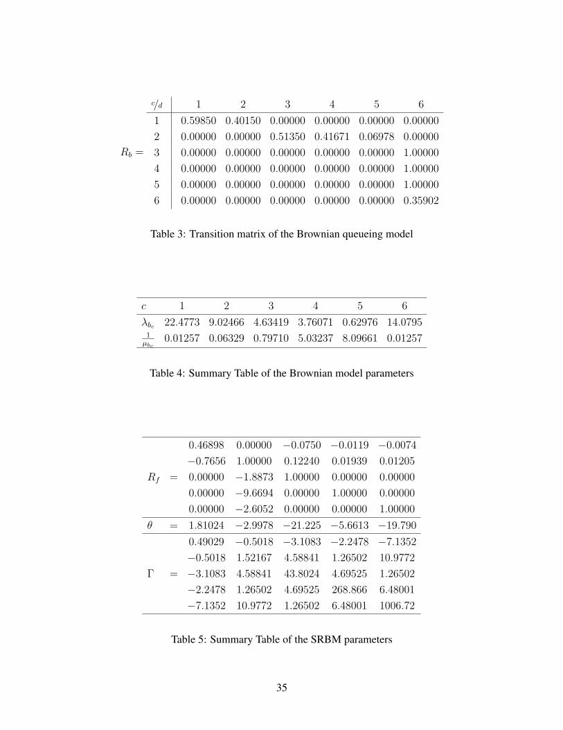
position approach. In the end, we obtain the routing matrix presented in Table 3. A summary of the

other model parameters may be found in Table 4. Where µbc denotes the aggregate effective ser-

vice time requirement (including outages) at each stage c (remark that 1/µb1 = 1/µb6 while outages

are assumed to occur during both initial and follow-up consultations).

Using these inputs, we will compute the SRBM approximating the workload process Z. The

three parameters associated with the SRBM Z∗ are presented in Table 5. Using these parameters we

show that the SRBM does exist. It is trivial to show that Γ is nondegenerate (while its eigenvectors

34

Rb =

c/d 1 2 3 4 5 6

1 0.59850 0.40150 0.00000 0.00000 0.00000 0.00000

2 0.00000 0.00000 0.51350 0.41671 0.06978 0.00000

3 0.00000 0.00000 0.00000 0.00000 0.00000 1.00000

4 0.00000 0.00000 0.00000 0.00000 0.00000 1.00000

5 0.00000 0.00000 0.00000 0.00000 0.00000 1.00000

6 0.00000 0.00000 0.00000 0.00000 0.00000 0.35902

Table 3: Transition matrix of the Brownian queueing model

c 1 2 3 4 5 6

λbc 22.4773 9.02466 4.63419 3.76071 0.62976 14.07951µbc

0.01257 0.06329 0.79710 5.03237 8.09661 0.01257

Table 4: Summary Table of the Brownian model parameters

0.46898 0.00000 −0.0750 −0.0119 −0.0074

−0.7656 1.00000 0.12240 0.01939 0.01205

Rf = 0.00000 −1.8873 1.00000 0.00000 0.00000

0.00000 −9.6694 0.00000 1.00000 0.00000

0.00000 −2.6052 0.00000 0.00000 1.00000

θ = 1.81024 −2.9978 −21.225 −5.6613 −19.790

0.49029 −0.5018 −3.1083 −2.2478 −7.1352

−0.5018 1.52167 4.58841 1.26502 10.9772

Γ = −3.1083 4.58841 43.8024 4.69525 1.26502

−2.2478 1.26502 4.69525 268.866 6.48001

−7.1352 10.9772 1.26502 6.48001 1006.72

Table 5: Summary Table of the SRBM parameters

35

are linearly independent). Hence the only remaining prerequisite is to provide a sufficient condition

that shows that Rf has the completely-S property. Simple arithmetics demonstrate that Rf is a P -

matrix (indicating that all its principal minors are positive). As such, sufficient conditions are met

forRf to possess the completely-S property (Chen et al., 2002). Therefore we can reasonably infer

the SRBM to exist.

Using the QNET software (Dai et al., 1992) we can now compute the stationary means of the

SRBM Z∗ that corresponds to the parameters recorded in Table 5. Let zi denote the stationary

mean of the SRBM Z∗ at workstation i. We have that the average number of patients present at

workstation i (in queue and in process) equals:

Qi = ziµi (64)

Using Little’s law we find that the average time spent at workstation i (including both waiting time

and servicing) equals:

E [WBrownian] =Qi

λi(65)

The performance of this model will be discussed in the next section.

VALIDATION OF THE MODEL THROUGH SIMULATION

We modeled the orthopaedic department by means of discrete event simulation. We used the Arena

software package, a discrete event simulator which allows for maximum customizability (Law &

Kelton, 2000; Kelton, Sadowski, & Sturrock, 2004). The use of simulation is widespread, even in

healthcare research. An extensive overview of the use of discrete-event simulation in healthcare

literature can be found with Jacobson et al. (2006). Compared to analytical approaches (such

as queueing models), simulation has the advantage of offering enormous amounts of modeling

freedom (the obligatory drawback being that one partially loses model adaptability as well as the

deeper understanding of the system dynamics at work).

36

i 1 2 3 4 5

Analytical models1µi

0.01257 0.06329 0.79710 5.03237 8.09661

ρi 0.99543 0.97854 0.14776 0.75701 0.20396

C2si

0.65079 0.60612 14.0786 1.98721 23.4125

C2ai

1.03176 0.91465 0.80444 0.84130 0.97343

pi 0.99139 0.96804 < 0.0001 0.13096 < 0.0001

E [WKingman] 5.05894 3.95430 0.79710 5.24027 8.09687

E [WWhitt] 5.05911 3.95298 0.79710 5.20325 8.09664

E [WBrownian] 7.72261 5.41723 0.27924 1.19658 5.00118

i 1 2 3 4 5

Simulation1µi

0.01257 0.06329 0.79711 5.03233 8.10131

ρi 0.99541 0.97858 0.14775 0.75701 0.20414

C2si

0.65796 0.60589 14.0969 1.98918 23.9050

C2ai

0.95046 0.92106 1.01075 0.68195 0.96212

E [WSimulation] 5.40098 3.46204 0.79711 5.11928 8.10131

Table 6: Summary Table of the model results

The simulation model operates under the same structure, assumptions and parameter values as

the ones used for the queueing models. Consequently, the simulation model can be used for valida-

tion purposes. The run length of the simulations guarantees the required statistical accuracy. The

resulting performance measures of the simulation model are presented in Table 6 (time-related

parameters are expressed in terms of days). First of all one can observe that traditional decom-

position approaches perform best. The Brownian queueing model on the other hand yields poor

approximations at each of the workstations. With respect to the workstations that experienced only

moderate or even light traffic, such inaccuracies were to be expected. Less obvious is the lack of

accuracy observed at the heavily loaded workstations (i.e. consultation and surgery). However, it

has been argued in literature that multiclass open re-entry networks are liable to inaccurate evalu-

ation of performance measures (Chen et al., 2002). These findings suggest that current Brownian

queueing models are not the most reliable tool to study complex hospital systems (i.e. systems that

37

are characterized by a multiclass client base and re-entry at previous stages of the service process).

Furthermore we note that the Kingman procedure offers a fairly accurate estimate of the flow time.

The same holds for the Whitt procedure. Unfortunately, the Whitt procedure is computationally

much more demanding.

We can observe that flow times of an average patient at consultation and surgery typically

amounts to 5.4 and 3.5 days respectively (remark that the time between service completion and

the making of a new appointment is not included). Squared coefficients of variation of the ser-

vice times at these workstations are comparable to those reported in literature. Notice that our

procedure, developed to approximate the variance of the aggregate service times including the

impact of outages, performs well. With respect to the wards we note large differences. As was

expected, patients visiting the third workstation (day hospital) have a flow time smaller than a day.

At the other wards, flow times are substantially larger while the recovery process of patients vis-

iting these workstations is more demanding. The difference in flow time between the internal and

external ward can be assigned to a number of reasons. First of all, the volume of patients recov-

ering at an external ward is relatively small (230 patients per year). In addition, the occurrence

of complications during the treatment process may result in a prolonged recovery process at an

external ward. Furthermore, we can observe relatively large squared coefficients of variation of the

service times at each of the wards. Due to the heterogeneity of the patient population, the recovery

process of two patients may deviate substantially. For instance, we already mentioned that the

JLoS of patients belonging to APR-DRG 302 ranges from 14 to 55 days (the difference between

patients suffering from different pathologies is even more outspoken). Finally, with respect to the

squared coefficients of variation of the interarrival times, on can note that most workstations ex-

perience Poisson-like arrivals. Bearing in mind the findings of Palm (1943) and Khinchin (1960),

this should not come as a surprise.

38

COMPUTATIONAL EXPERIMENTS AND WHAT-IF ANALYSIS

In this section we focus on the performance of the consultation workstation. Similar analysis is

possible for the other workstations, however, we focus on consultation because all types of outages

are applicable to that workstation. We investigate the impact of consultation block size (n) as

well as mean and variance of outages and resolve times (i.e. τr, τi, 1/µs, σ2r and σ2

s ) on patient flow

times. A number of what-if scenarios will be evaluated and compared using both queueing analysis

and simulation. Queueing models, though difficult to develop, are fast and easy to implement.

Therefore, what-if question can be answered in no time.

In a first section we define a number of performance indicators. The ensuing sections deal with

the scenarios studied and a final section discusses the results of the different scenarios.

Defining Performance Indicators

The comparison between scenarios is based on the following factors:

• Patient total expected waiting time (i.e. the expected flow time of an average patient),

• ratio of time spent on absences (κs),

• ratio of time spent on resolving interrupts (κf ),

• the effective utilization rate at the consultation workstation (ρ1).

Patient waiting time as well as effective utilization rate have already been discussed, the ratio

of time spent on absences and the time spent on resolving interrupts however still requires some

explanation. The average effective service time at the consultation workstation can be divided into

three components:

• Natural service time (1/ν1),

• outage time due to unscheduled absences (1/µs),

39

• outage time due to service interruptions (1/µg).

Together these parameters add up to the average effective service time as is experienced by a

patient:1

φ=

1

ν1

+1

µs+

1

µg(66)

Remark that including the scaling due to the availability of the consultation workstation (A1) does

not impact the ratios (while all elements would be scaled by an equal factor). Therefore, scaling is

not taken into account. In what follows, we will use these three components to construct a number

of performance ratios.

First we have a look at the ratio of time spent on absence. We compute this measure by relating

natural service time to time spent on absence. More specifically:

κs =ν1

nµs(67)

Where (1/nµs) is the average time spent on absences per patient. Remark that, while natural service

time remains the same over each of the scenarios, the ratio can be used to evaluate the amount of

time spent on absence in each of the scenarios (thereby enabling the comparison over the different

scenarios). With respect to the ratio expressing the time spent on resolving interrupts, a similar

logic can be applied. We can express the amount of time spent on resolving interrupts as follows:

1µg

= Eν1 [EJ0 [. . . EJl [. . . [S0 + . . .+ Sl + . . .] . . .] . . .]]

= 1ν1τrτi

(1 + τr

τi+ . . .+ τ lr

τ li+ . . .

)= 1

ν1τr

τi−τr

(68)

Relating 1/µg and 1/ν1 results in:

κf =τr

τi − τr(69)

40

Scenarios Involving The Impact of Interrupts

Interrupts can exert influence on patient flow times by means of:

• The number of interrupts; the time between two consecutive interrupts (i.e. τi),

• the time required to resolve an interrupt (τr),

• the variance of these resolve times (σ2r ).

The scenarios are summarized in Table 7 (scenario 0 corresponds to the base case discussed in

earlier sections). Scenarios 1 and 2 focus on the impact of the number of interrupts, scenarios

3 and 4 on the resolve times, and scenarios 5 and 6 study the effect of variability of the resolve

times. Over the different scenarios the impact of the parameters of interest is gradually reduced

(e.g. scenarios 1 and 2 have a smaller number of interrupts during consultation service).

The impact of interrupts on medical practice has been observed by Harvey, Jarrett, and Pel-

tekian (1994), Lehaney and Clarke (1999), Chisholm et al. (2001), Brixey, Walji, Zhang, Johnson,

and Turley (2004), France et al. (2005), Volpp and Grande (2006), Tucker and Spear (2006), and

Gabow et al. (2006) among others. All agree on the detrimental effects of interrupts on patient

flow time. In addition, they provide several valuable insights to control and decrease the impact

of interrupts. For instance, Harvey et al. (1994) suggest the pooling of paging of doctors (next to

telephone calls, paging calls are one of the largest sources of interrupts) in order to decrease vari-

ability in individual paging patterns. France et al. (2005) propose the use of information systems

(e.g. an electronic whiteboard) and team training to enhance performance. Tucker et al. (2006)

suggest the redesign of treatment processes (e.g. outsourcing of administrative tasks) in order to

make service more robust against preemptive outages. In addition Tucker et al. (2006) and Volpp

et al. (2006) propose the filtering of non-urgent communication towards medical staff.

Scenarios Involving The Impact of Absences

Similar to interrupts, absences impact patient flow times in three different ways:

41

• The consultation block size (i.e. n), which controls the number of absences,

• the duration of absence times (1/µs),

• the variance of absence times (σ2s ).

Scenarios 7 and 8 focus on the number of absences, scenarios 9 and 10 deal with the impact of

absence times, and scenarios 11 and 12 assess the effect of variability of absence times. Once

more, the impact of the parameters is gradually decreased over the different scenarios.

The impact of absences is discussed in Babes et al. (1991), Liu et al. (1998a), Liu and Liu

(1998b), Easton et al. (2005). There is a general agreement on the disruptive effect of absences on

patient flow time. Easton et al. (2005) identify robust staffing, scheduling and recovery practices

to minimize the effects of absences. Liu et al. (1998b) acknowledge the importance of block size

and propose a what-if simulation approach in order to determine the best block size. In fact, the

relationship between block size and patient flow time is similar to the relationship between batch

size and waiting time (in the presence of setups between batches). As such the convex relationship

first described by Karmarkar (1987) may also be observed here. In this view, Vandaele et al.

(2003b) determine the optimal size of patient groups queueing in front of a nuclear resonance

scanner.

Queueing and Simulation Results

Before advancing to some numerical results, we first present two graphs illustrating the effect of

outages on total patient waiting times. In Figure 6 and Figure 7, we plot the relation between

average patient flow times and the utilization rate. Figure 6 deals with utilization rates ranging

over a large spectrum of possible values. Figure 7 on the other hand focusses on a smaller range in

order to magnify the differences between the modeling approaches (i.e. Figure 7 is a more detailed

representation of a part of Figure 6). Remark that the order of scenarios is lost while they are

plotted in function of increasing utilization rates. The graphs show that parametric decomposition

approaches are capable to provide an accurate approximation of patient flow times at the consul-

42

Figure 6: Patient waiting times at consultation in function of utilization rates (extended range)

Figure 7: Patient waiting times at consultation in function of utilization rates (limited range)

43

Scenario 0 1 2 3 4 5 6

ρ1 0.9954 0.9877 0.9809 0.9874 0.9794 0.9954 0.9954

κs 0.0506 0.0506 0.0506 0.0506 0.0506 0.0506 0.0506

κf 0.1707 0.1613 0.1528 0.1608 0.1511 0.1707 0.1707

E [WKingman] 5.0589 1.8948 1.1220 1.8323 1.1320 5.0389 5.0377

E [WWhitt] 5.0591 1.8950 1.1220 1.8324 1.1320 5.0391 5.0378

E [WBrownian] 7.7226 2.8528 1.7742 2.7802 1.6404 7.6498 7.6721

E [WSimulation] 5.4010 2.0537 1.2873 1.9584 1.1875 5.3637 5.3544

Scenario 7 8 9 10 11 12

ρ1 0.9935 0.9917 0.9935 0.9914 0.9954 0.9954

κs 0.0482 0.0460 0.0482 0.0456 0.0506 0.0506

κf 0.1707 0.1707 0.1707 0.1707 0.1707 0.1707

E [WKingman] 3.5444 2.7882 3.5383 2.6884 5.0448 5.0141

E [WWhitt] 3.5445 2.7884 3.5385 2.6885 5.0450 5.0143

E [WBrownian] 5.3867 4.2809 5.4314 4.1252 7.7189 7.7110

E [WSimulation] 3.6201 2.9732 3.8690 2.8617 5.3863 5.3571

Table 7: Effect of decreasing the impact of outages on patient flow times

tation workstation. Brownian motion queueing models seem to be less accurate. In addition, both

graphs clearly illustrate the trade-off between utilization rate and patient flow time. In heavy traffic

systems (e.g. the majority of hospital systems), approaching system capacity gives rise to waiting

times that skyrocket. Conversely, even a small decrease in utilization yields substantial gains in

flow times. Hospital decision makers see themselves trapped in the trade-off between patient flow

times and the urge to utilize resources as much as possible. Through reducing the impact of out-

ages, management can drastically improve performance without compromising on patient volumes

and without expanding capacity.

The summary of performance measures of the different scenarios as well as those of the base

case (Scenario 0) is given in Table 7 (remark that patient flow times are expressed in days). We

can observe that decreasing the number of interrupts (scenarios 1 and 2) and reducing the time

spent on resolving interrupts (scenarios 3 and 4) results in a decrease of κf . In other words, the

proportion of time spent on resolving interrupts decreases. Therefore the utilization rate decreases

44

and consequently a substantial reduction in patient flow time is achieved. Further remark that

decreasing the number of interrupts and reducing the time spent on resolving interrupts have an

equivalent effect on patient flow time. When reducing the variance of the resolve times (scenarios

5 and 6), we observe no changes in the proportion of time spent on resolving interrupts (while

the mean resolve time remains the same). Nevertheless, the impact on patient flow times are

apparent; even if the same amount of time is spent on resolving interrupts, decreasing variability

of resolve times improves performance. When we have a look at scenarios 7 to 12, similar effects

are observed. The impact of reducing the effect of absences, however, is less outspoken while the

proportion of time spent on absences is smaller than that of time spent on resolving interrupts (i.e.

κs < κf ). As a result, focussing on the impact of interrupts will generate a larger impact.

These results highlight a number of key insights. First we have demonstrated that patient flow

times increase drastically when approaching system capacity. Therefore, hospital decision makers

should avoid high levels of utilization at hospital workstations. Second we have shown that inter-

rupts and absences have a devastating impact on performance. It is essential to limit their occur-

rence, their duration and the variance thereof. Finally the results indicate that decomposition-based

queueing models offer a valuable tool in assessing hospital performance. With respect to Brownian

queueing models, our experience indicates that current methodology is unable to provide reliable

performance measures of complex hospital systems (i.e. multiclass open re-entry networks).

CONCLUSIONS

In this paper we used a variety of modeling techniques to assess performance (in terms of patient

flow times) at the orthopaedic department of the Middelheim hospital. We showed that the queue-

ing models based on decomposition approaches outperform those that rely on Brownian motion

approximation. Decomposition-based models yield accurate results and as such they can be con-

sidered a valuable tool for hospital performance analysis. Using these models, we demonstrated

that hospitals operating under heavy traffic conditions face skyrocketing flow times. Therefore,

45

hospital decision makers should resist the urge to maximize occupancy levels of hospital facilities.

Using newly developed techniques, we have shown that service outages (doctor interruptions

and absences) have a devastating impact on patient flow times at heavily loaded workstations.

Nevertheless, hospital practice and literature often dismiss outages as insignificant, consider them

acceptable or ignore them altogether. While outages as individual occurrences have only limited

impact, together they pack a powerful punch. Potential improvements include the outsourcing

of administrative tasks, the careful selection of consultation block sizes and the implementing

of robust and proactive procedures. Reducing the effect of outages decreases flow times while

maintaining patient volumes and capacity structure. As such minimizing the impact of outages is

considered a key managerial challenge.

The contributions of this paper can be summarized as follows: (i) Several modeling approaches

are compared and insight is provided into which procedure is best at modeling complex hospital

systems; (ii) new expressions assessing the impact of service outages are developed; (iii) a compar-

ison between various scenarios, evaluating the impact of service outages in heavily loaded systems,

provides several important managerial insights.

As was illustrated in this paper, the modeling of healthcare systems differs substantially from

the modeling of manufacturing systems. Not all issues have been addressed in this paper. Improve-

ments may be made with respect to the modeling of time in queueing systems. Consultation and

surgery typically operate during predefined time blocks, whereas recovery is a continuous activity.

Combining both types of workstations in a single queueing network, proves to be a difficult task.

The presence of time blocks impacts the squared coefficients of variation of the arrivals and the

departures. Current queueing models do not account for this increase in variability. Moreover,

given the inherent high degree of variability in service times, hospitals often use flexible working

schedules that allow for overtime, variable server capacity and other deviations from the standard

queueing model topology. Such deviations add to the complexity of the problem, making ”time” a

major modeling issue.

46

References

Albin, S. (1984). Approximating a point process by a renewal process, II: superposition arrival

processes to queues. Operations Research, 32, pp 1133–1162.

Askin, R. (1993). Modeling and analysis of manufacturing systems. Wiley, New York.

Babes, M. & Sarma, G. (1991). Out-patient queues at the Ibn-Rochd health center. Journal of the

Operational Research Society, 42, pp 845–855.

Belson, D. (2006). Managing a patient flow improvement project. Springer Science, New York.

pp 151–187. In R.W. Hall: Patient flow: reducing delay in healthcare delivery.

Bitran, G. & Tirupati, D. (1988). Multiproduct queueing networks with deterministic routing:

decomposition approach and the notion of interference. Management Science, 34, pp 75–100.

Bramson, M. (1994). Instability of FIFO queueing networks. The Annals of Applied Probability,

4, pp 414–431.

Bramson, M. & Dai, J. (2001). Heavy traffic limits for some queueing networks. The Annals of

Applied Probability, 11, pp 49–90.

Bretthauer, K. (2004). Service management. Decision Sciences, 35, pp 325–332.

Brixey, J., Walji, M., Zhang, J., Johnson, T. & Turley, J. (2004). Proposing a taxonomy and

model of interruption. in K. Kurokawa, I. Nakajima & Y. Ishibashi (eds), Proceedings of 6th

International Workshop on Enterprise Networking and Computing in Healthcare Industry.

Healthcom. pp 184–188.

Cayirli, T. & Veral, E. (2003). Outpatient scheduling in health care: a review of literature. Produc-

tion and Operation Management, 12, pp 519–549.

Cerda, E., de Pablos, L. & Rodriguez, M. (2006). Waiting lists for surgery. Springer Science, New

York. pp 151–187. In R.W. Hall: Patient flow: reducing delay in healthcare delivery.

47

Chen, H. & Shen, X. (2003). Computing the stationary distribution of an SRBM in an orthant with

applications to queueing networks. Queueing Systems, 45, pp 27–45.

Chen, H., Shen, X. & Yao, D. (2002). Brownian approximations of multiclass open-queueing

networks. Operations Research, 50, pp 1032–1049.

Chisholm, C., Collison, E., Nelson, D. & Cordell, W. (2000). Emergency department workplace

interruptions: are emergency physicians ”interrupt-driven” and ”multitasking”. Academic

Emergency Medicine, 7, pp 1239–1243.

Chisholm, C., Dornfeld, A., Nelson, D. & Cordell, W. (2001). Work interrupted: a comparison

of workplace interruptions in emergency departments and primary care offices. Annals of

Emergency Medicine, 38, pp 146–151.

Cots, F., Elvira, D., Castells, X. & Dalmau, E. (2000). Medicare’s DRG-weights in a European

environment: the Spanish experience. Health Policy, 51, pp 31–47.

Dai, J. (1995). On positive Harris recurrence of multiclass queueing networks: a unified approach

via fluid limit models. Annals of Applied Probability, .

Dai, J. & Harrison, J. (1991). Steady-state analysis of RBM in a rectangle: numerical methods and

a queueing application. The Annals of Applied Probability, 1, pp 16–35.

Dai, J. & Harrison, J. (1992). Reflected Brownian motion in an orthant: numerical methods for a

steady-state analysis. The Annals of Applied Probability, 2, pp 65–86.

Dai, J. & Harrison, J. (1993). The QNET method for two-moment analysis of closed manufacturing

systems. The Annals of Applied Probability, 3, pp 968–1012.

Dai, J. & Jennings, O. (2003). Stochastic Models and Optimizations. Springer, New York.

Dai, J. & Kurtz, T. (1995). A multiclass station with markovian feedback in heavy traffic. Mathe-

matics of Operations Research, .

48

Dai, J., Nguyen, V. & Reiman, M. (1994). Sequential bottleneck decomposition: an approximation

method for generalized Jackson networks. Operations research, 42, pp 119–136.

Dai, J. & Weiss, G. (1996). Stability and instability of fluid models for re-entrant lines. Mathemat-

ics of Operations Research, 21, pp 115–135.

Dai, J., Yeh, D. & Zhou, C. (1997). The QNET method for re-entrant queueing networks with

priority disciplines. Operations Research, 45, pp 610–623.

Dudewicz, E. & Mishra, S. (1988). Modern mathematical statistics. John Wiley Sons, New York.

Easton, F. & Goodale, J. (2005). Schedule recovery: unplanned absences in service operations.

Decision Sciences, 36, pp 459–488.

Federgruen, A. & Green, L. (1986). Queueing systems with service interruptions. Operations

Research, 34, pp 752–768.

Fetter, R. (1991). Diagnosis related groups: understanding hospital performance. Interfaces,

21, pp 6–26.

France, D., Levin, S., Hemphill, R., Chen, K., Rickard, D., Makowski, R., Jones, I. & Aronsky,

D. (2005). Emergency physicians’ behaviors and workload in the precense of an electronic

whiteboard. International Journal of Medical Informatics, 74, pp 827–837.

Gabow, P., Karkhanis, A., Knight, A., Dixon, P., Eiser, S. & Albert, R. (2006). Observations

of residents’ work activities for 24 consecutive hours: implications for workflow redesign.

Academic Medecine, 81, pp 766–775.

Green, L. (2003). How many hospital beds. Inquiry, 39, pp 400–412.

Green, L. (2006). Queueing analysis in health care. Springer Science, New York. pp 281–307. In

R.W. Hall: Patient flow: reducing delay in healthcare delivery.

49

Hall, R., Belson, D., Muralli, P. & Dessouky, M. (2006). Modeling patient flows through the

healthcare system. Springer Science, New York. pp 1–44. In R.W. Hall: Patient flow: reduc-

ing delay in healthcare delivery.

Haque, L. & Armstrong, M. (2007). A survey of the machine interference problem. European

Journal of Operational Research, 179, pp 469–482.

Harper, P. (2002). A framework for operational modelling of hospital resources. Health care

management science, 5, pp 165–173.

Harrison, J. (1988). Brownian models of queueing networks with heterogenous customer

populations. Stochastic Differential Systems, Stochastic Control Theory and Application,

10, pp 146–186.

Harrison, J. & Pich, M. (1996). Two-moment analysis of open queueing networks with general

workstation capabilities. Operations Research, 44, pp 936–950.

Harrison, J. & Williams, R. (1987). Multidimensional reflected Brownian motions having expo-

nential stationary distributions. The Annals of Probability, 15, pp 115–137.

Harrison, J. & Williams, R. (1992). Brownian models of feedforward queueing networks: quasire-

versibility and product form solutions. Annals of Applied Probability, 2, pp 263–293.

Harvey, R., Jarrett, P. & Peltekian, K. (1994). Patterns of paging medical interns during night calls

at two teaching hospitals. Canadian Medical Association Journal, 151, pp 307–311.

Haskose, A., Kingsman, B. & Worthington, D. (2002). Modelling flow and jobbing shops as

a queueing network for workload control. International Journal of Production Economics,

78, pp 271–285.

Hopp, W. & Spearman, L. (2000). Factory Physics. 2 edn. McGraw-Hill Higher Education, New

York.

50

Jackson, J. (1957). Network of waiting lines. Operations Research, 5, pp 518–521.

Jackson, J. (1963). Jobshop-like queueing systems. Management Science, 10, pp 131–142.

Jacobson, S., Hall, S. & Swisher, J. (2006). Discrete-event simulation of health care systems.

Springer Science, New York. pp 211–252. In R.W. Hall: Patient flow: reducing delay in

healthcare delivery.

Kao, E. & Tung, G. (1981). Bed allocation in a public health care delivery system. Management

Science, 27, pp 507–520.

Karmarkar, U. (1987). Lot sizes, lead times and in-process inventories. Management Science,

33, pp 409–418.

Kelton, W., Sadowski, R. & Sturrock, D. (2004). Simulation with Arena. 3 edn. McGraw-Hill,

New York.

Khinchin, A. (1960). Mathematical Methods in the Theory of Queueing. Hafner, New York.

Koizumi, N., Kuno, E. & Smith, T. (2005). Modeling patient flows using a queueing network with

blocking. Health Care Management Science, 8, pp 49–60.

Lambrecht, M., Ivens, P. & Vandaele, N. (1998). Aclips: a capacity and lead time integrated

procedure for scheduling. Management Science, 44, pp 1548–1561.

Law, A. & Kelton, W. (2000). Simulation Modeling and Analysis. 3 edn. McGraw-Hill, New York.

Lehaney, B., Clarke, S. & Paul, R. (1999). A case of intervention in an outpatient department.

Journal of the Operational Research Society, 50, pp 877–891.

Liu, L. & Liu, X. (1998a). Block appointment systems for outpatient clinics with multiple doctors.

The Journal of the Operational Research Society, 49, pp 1254–1259.

Liu, L. & Liu, X. (1998b). Dynamic and static job allocation for multi-server systems. IIE Trans-

actions, 30, pp 845–854.

51

McLaughlin, C. (1996). Why variation reduction is not everything: a new paradigm for service

operations. International Journal of Service Industry Management, 7, pp 17–30.

McManus, M., Long, M., Cooper, A. & Litvak, E. (2004). Queueing theory accurately models the

need for critical care resources. Anesthesiology, 100, pp 1271–1276.

Nguyen, V. (1995). Fluid and diffusion approximations of a two-station mixed queueing network.

Mathematics of Operations Research, 20, pp 321–354.

Palm, C. (1943). Intensittsschwankungen im fernsprechverkehr. Ericsson Technics, 44, pp 1–89.

Reiman, M. (1984). Open queueing networks in heavy traffic. Mathematics of Operations Re-

search, 9, pp 441–458.

Roth, A. & Van Dierdonck, R. (1995). Hospital resource planning: concepts, feasibility and frame-

work. Production and Operations Meanagement, 4, pp 2–29.

Sethuraman, K. & Tirupati, D. (2005). Evidence of bullwhip effect in healthcare sector: causes,

consequences and cures. International Journal of Services and Operations Management,

1(4), pp 372–394.

Shanthikumar, J. & Buzacott, J. (1981). Open queueing network models of dynamic job shops.

International Journal of Production Research, 19, pp 255–266.

Stecke, K. & Aronson, J. (1985). Review of operator/machine interference models. Journal of

Production Research, 23, pp 129–151.

Stidham, S. (2002). Analysis, design and control of queueing systems. Operations Research,

50, pp 197–216.

Sutherland, J. & Botz, C. (2006). The effect of misclassification errors on case mix measurement.

Health Policy, 79, pp 195–202.

52

Tsikriktsis, N. & Heineke, J. (2004). The impact of process variation on customer dissatisfaction:

evidence from the u.s. domestic airline industry. Decision Sciences, 35, pp 129–142.

Tucker, A. & Spear, S. (2006). Operational failures and interruptions in hospital nursing. Health

Services Research, 41, pp 643–662.

van Merode, G., Groothuis, S. & Hasman, A. (2004). Enterprise resource planning for hospitals.

International Journal of Medical Informatics, 73, pp 493–501.

Vandaele, N. & De Boeck, L. (2003). Advanced resource planning. Robotics and Computer Inte-

grated Manufacturing, 19, pp 211–218.

Vandaele, N., De Boeck, L. & Callewier, D. (2002). An open queueing network for lead time

analysis. IIE Transactions, 34, pp 1–9.

Vandaele, N., Van Nieuwenhuyse, I. & Cupers, S. (2003). Optimal grouping for a nuclear magnetic

resonance scanner by means of an open queueing model. European Journal of Operational

Research, 151, pp 181–192.

Vissers, J., Bertrand, J. & De Vries, G. (2001). A framework for production control in health care

organizations. Production Planning & Control, 12, pp 591–604.

Volpp, K. & Grande, D. (2006). Residents’ suggestions for reducing errors in teaching hospitals.

The New England Journal of Medicine, 348, pp 851–855.

Whitt, W. (1983). The queueing network analyzer. The Bell System Technical Journal,

62, pp 2779–2815.

Whitt, W. (1993). Approximations for the GI/G/m queue. Productions and Operations Manage-

ment, 2, pp 114–161.

Whitt, W. (1999). Partitioning customers into service groups. Management Science, 45, pp 1579–

1592.

53

Worthington, D. (1987). Queueing models for hospital waiting lists. The Journal of the Operational

Research Society, 38, pp 413–422.

Worthington, D. (1991). Hospital waiting list management models. The Journal of the Operational

Research Society, 42, pp 833–843.

Zhu, Z., Sivakumar, K. & Parasuraman, A. (2004). A mathematical model of service failure and

recovery strategies. Decision Sciences, 35, pp 493–525.

54