Modelica - A Uniﬁed Object-Oriented Language for System Modeling · PDF file ·...

Modelica - A Unified Object-Oriented Language forSystem Modeling and Simulation

Peter Fritzson and Vadim Engelson

PELAB, Dept. of Computer and Information ScienceLinköping University, S-58183, Linköping, Sweden

{petfr,vaden}@ida.liu.se

Abstract. A new language called Modelica for hierarchical physical modeling isdeveloped through an international effort. Modelica 1.0 [http://www.Dynasim.se/Modelica] was announced in September 1997. It isan object-oriented language for modeling of physical systems for the purpose ofefficient simulation. The language unifies and generalizes previous object-ori-ented modeling languages. Compared with the widespread simulation languagesavailable today this language offers three important advances: 1) non-causalmodeling based on differential and algebraic equations; 2) multidomain mode-ling capability, i.e. it is possible to combine electrical, mechanical, thermody-namic, hydraulic etc. model components within the same application model; 3) ageneral type system that unifies object-orientation, multiple inheritance, andtemplates within a single class construct.A class in Modelica may contain variables (i.e. instances of other classes), equa-tions and local class definitions. A function (method) can be regarded as a spe-cial case of local class without equations, but including an algorithm section.The equation-based non-causal modeling makes Modelica classes more reusablethan classes in ordinary object-oriented languages. The reason is that the classadapts itself to the data flow context where it is instantiated and connected. Themulti-domain capability is partly based on a notion of connectors, i.e. certainclass members that can act as interfaces (ports) when connecting instantiatedobjects. Connectors themselves are classes just like any other entity in Modelica.Simulation models can be developed using a graphical editor for connection dia-grams. Connections are established just by drawing lines between objects pickedfrom a class library.The Modelica semantics is defined via translation of classes, instances and con-nections into a flat set of constants, variables and equations. Equations are sortedand converted to assignment statements when possible. Strongly connected setsof equations are solved by calling a symbolic and/or numeric solver. The gener-ated C/C++ code is quite efficient.In this paper we present the Modelica language with emphasis on its class con-struct and type system. A few short examples are given for illustration and com-pared with similar constructs in C++ and Java when this is relevant.

1 Introduction

1.1 Requirements for a modeling and simulation language

The use of computer simulation in industry is rapidly increasing. This is typically used

E. Jul (Ed.): ECOOP’98, LNCS 1445, pp. 67-90, 1998. c Springer-Verlag Heidelberg Berlin 1998

to optimize products and to reduce product development cost and time. Whereas in thepast it was considered sufficient to simulate subsystems separately, the current trend isto simulate increasingly complex physical systems composed of subsystems from mul-tiple domains such as mechanic, electric, hydraulic, thermodynamic, and control sys-tem components.

1.2 Background

Many commercial simulation software packages are available. The market is dividedinto distinct domains, such as packages based on block diagrams (block-oriented tools,such as SIMULINK[18], System Build, ACSL[19]), electronic programs (signal-ori-ented tools, such as SPICE[20], Saber), multibody systems (ADAMS[21], DADS,SIMPACK), and others. With very few exceptions, all simulation packages are strongonly in one domain and are not capable of modeling components from other domainsin a reasonable way. However, this is a prerequisite to be able to simulate modern prod-ucts that integrate, e.g., electric, mechanic, hydraulic and control components. Tech-niques for general purpose physical modeling have been developed some decades ago,but did not receive much attention from the simulation market due to lacking computerpower at that time.

To summarize, we currently have three following problems:

• High performance simulation of complex multi-domain systems is needed. Currentwidespread methods cannot cope with serious multi-domain modeling andsimulation.

• Simulated systems are increasingly complex. Thus, system modeling has to bebased primarily on combining reusable components. A better technology is neededin creating easy-to-use reusable components.

• It is hard to achieve truly reusable components in object-oriented programming andmodeling

Disadvantage of block-oriented tools is the gap between the physical structure of somesystem and structure of corresponding model created by the tool. In block-oriented toolsthe model designer has to predict in advance in which way the equations will be used.It reduces reusability of model libraries and causes incompatibilities between blocks.

1.3 Proposed solution

The goal of the Modelica project[23] is to provide practically usable solutions to theseproblems, based on techniques for mathematical modeling of reusable components.

Several first generation object-oriented mathematical modeling languages andsimulation systems (ObjectMath [11,13], Dymola [4], Omola [2], NMF [12], gPROMS[3], Allan [6], Smile [5] etc.) have been developed during the past few years. Theselanguages were applied in areas such as robotics, vehicles, thermal power plants,nuclear power plants, airplane simulation, real-time simulation of gear boxes, etc.

68 Peter Fritzson and Vadim Engelson

Several applications have shown, that object-oriented modeling techniques is notonly comparable to, but outperform special purpose tools on applications that are farbeyond the capacity of established block-oriented simulation tools.

However, the situation of a number of different incompatible object-orientedmodeling and simulation languages was not satisfactory. Therefore in the fall of 1996a group of researchers (see Sect. 3.6) from universities and industry started worktowards standardization and making this object-oriented modeling technology widelyavailable.

The new language was called Modelica and designed for modeling dynamicbehavior of engineering systems, intended to become a de facto standard.

Modelica is superior to current technology mainly for the following reasons:

• Object-oriented modeling. This technique makes it possible to create physicallyrelevant and easy-to-use model components, which are employed to supporthierarchical structuring, reuse, and evolution of large and complex models coveringmultiple technology domains.

• Non-causal modeling. Modeling is based on equations instead of assignmentstatements as in traditional input/output block abstractions. Direct use of equationssignificantly increases re-usability of model components, since components adaptto the data flow context in which they are used. This generalization enables bothsimpler models and more efficient simulation.

• Physical modeling of multiple domains. Model components can correspond tophysical objects in the real world, in contrast to established techniques that requireconversion to “signal” blocks with fixed input/output causality. In Modelica thestructure of the model becomes more natural in contrast to block-oriented modelingtools. For application engineers, such “physical” components are particularly easyto combine into simulation models using a graphical editor.

1.4 Modelica view of object-orientation

Traditional object-oriented languages like C++, Java and Simula support programmingwith operations on state. The state of the program includes variable values and objectdata. Number of objects changes dynamically. Smalltalk view of object orientation issending messages between (dynamically) created objects. The Modelica approach isdifferent. The Modelica language emphasizes structured mathematical modeling anduses structural benefits of object-orientation. A Modelica model is primarily a declara-tive mathematical description, which allows analysis and equational reasoning. Forthese reasons, dynamic object creation at runtime is usually not interesting from a math-ematical modeling point of view. Therefore, this is not supported by the Modelica lan-guage.

To compensate this missing feature arrays are provided by Modelica. An array isan indexed set of objects of equal type. The size of the set is determined once at runtime.This construct for example can be used to represent a set of similar rollers in a bearing,or a set of electrons around an atomic nucleus.

69Modelica

1.5 Object-Oriented Mathematical Modeling

Mathematical models used for analysis in scientific computing are inherently complexin the same way as other software. One way to handle this complexity is to use object-oriented techniques. Wegner [7] defines the basic terminology of object-oriented pro-gramming:

• Objects are collections of operations that share a state. These operations are oftencalled methods. The state is represented by instance variables, which are accessibleonly to the operation’s of the object.

• Classes are templates from which objects can be created.

• Inheritance allows us to reuse the operations of a class when defining new classes.A subclass inherits the operations of its parent class and can add new operations andinstance variables.

Note that Wegner’s strict requirement regarding data encapsulation is not fulfilled byobject oriented languages like Simula or C++, where non-local access to instance vari-ables is allowed.

More important, while Wegner’s definitions are suitable for describing the notionsof object-oriented programming, they are too restrictive for the case of object-orientedmathematical modeling, where a class description may consist of a set of equations,which implicitly define the behavior of some class of physical objects or therelationships between objects. Functions should be side-effect free and regarded asmathematical functions rather than operations. Explicit operations on state can becompletely absent, but can be present. Also, causality, i.e. which variables are regardedas input, and which ones are regarded as output, is usually not defined by such anequation-based model.

There are usually many possible choices of causality, but one must be selectedbefore a system of equations is solved. If a system of such equations is solvedsymbolically, the equations are transformed into a form where some (state) variablesare explicitly defined in terms of other (state) variables. If the solution process isnumeric, it will compute new state variables from old variable values, and thus operateon the state variables. Below we define the basic terminology of object-orientedmathematical modeling:

• An object is a collection of variables, equations, functions and other definitionsrelated to a common abstraction and may share a state. Such operations are oftencalled methods. The state is represented by instance variables.

• Classes are templates from which objects or subclasses can be created.

• Inheritance allows us to reuse the equations, functions and definitions of a classwhen defining objects and new classes. A subclass inherits the definitions of itsparent class and can add new equations, functions, instance variables and otherdefinitions.

As previously mentioned, the primary reason to introduce object-oriented techniques in


mathematical modeling is to reduce complexity. To explain these ideas we use some ex-amples from the domain of electric circuits. When a mathematical description is de-signed, and it consists of hundreds of equations and formulae, for instance a model of acomplex electrical system, structuring the model is highly advantageous.

2 A Modelica overview

Modelica programs are built from classes. Like in other object-oriented languages,class contains variables, i.e. class attributes representing data. The main differencecompared with traditional object-oriented languages is that instead of functions (meth-ods) we use equations to specify behavior. Equations can be written explicitly, likea=b, or be inherited from other classes. Equations can also be specified by the con-nect statement. The statement connect(v1, v2) expresses coupling between vari-ables v1 and v2. These variables are called connectors and belong to the connected ob-jects. This gives a flexible way of specifying topology of physical systems described inan object-oriented way using Modelica.

In the following sections we introduce some basic and distinctive syntactical andsemantic features of Modelica, such as connectors, encapsulation of equations,inheritance, declaration of parameters and constants. Powerful parametrizationcapabilities (which are advanced features of Modelica) are discussed in Sect. 2.10.

2.1 Modelica model of an electric circuit

As an introduction to Modelica we will present a model of a simple electrical circuit asshown in Fig. 1. The system can be broken into a set of connected electrical standardcomponents. We have a voltage source, two resistors, an inductor, a capacitor and aground point. Models of such components are available in Modelica class libraries.

Fig. 1. A connection diagram of the simple electrical circuit example. The numbers of wires andnodes are used for reference in Table 3.1.

A declaration like one below specifies that R1 to be of class Resistor and setsthe default value of the resistance, R, to 10.

Resistor R1(R=10);

R1

u (t)

C

R2

LAC

G

N1

N2

N3 N4

++

++

+

1

2

3

4

5

67

Legend

AC, R1, R2, L, C, G - circuit elementsN1-N4 - nodes1-7 - wires

- positive pins+u (t) = VA sin(2π f t)

(alternate voltage source)

71Modelica

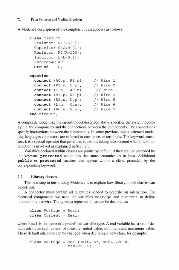
A Modelica description of the complete circuit appears as follows:

class circuit Resistor R1(R=10); Capacitor C(C=0.01); Resistor R2(R=100); Inductor L(L=0.1); VsourceAC AC; Ground G;

equationconnect (AC.p, R1.p); // Wire 1connect (R1.n, C.p); // Wire 2connect (C.n, AC.n); // Wire 3connect (R1.p, R2.p); // Wire 4connect (R2.n, L.p); // Wire 5connect (L.n, C.n); // Wire 6connect (AC.n, G.p); // Wire 7

end circuit;

A composite model like the circuit model described above specifies the system topolo-gy, i.e. the components and the connections between the components. The connectionsspecify interactions between the components. In some previous object-oriented mode-ling languages connectors are referred to cuts, ports or terminals. The keyword con-nect is a special operator that generates equations taking into account what kind of in-teraction is involved as explained in Sect. 2.3.

Variables declared within classes are public by default, if they are not preceded bythe keyword protected which has the same semantics as in Java. Additionalpublic or protected sections can appear within a class, preceded by thecorresponding keyword.

2.2 Library classesThe next step in introducing Modelica is to explain how library model classes can

be defined.A connector must contain all quantities needed to describe an interaction. For

electrical components we need the variables voltage and current to defineinteraction via a wire. The types to represent those can be declared as

class Voltage = Real;class Current = Real;

where Real is the name of a predefined variable type. A real variable has a set of de-fault attributes such as unit of measure, initial value, minimum and maximum value.These default attributes can be changed when declaring a new class, for example:

class Voltage = Real(unit=”V”, min=-220.0,max=220.0);


In Modelica, the basic structuring element is a class. There are seven restricted classcategories with specific keywords, such as type (a class that is an extension of built-in classes, such as Real, or of other defined types) and connector (a class that doesnot have equations and can be used in connections). In any model the type and con-nector keywords can be replaced by the class keyword giving a semanticallyequivalent model. Other specific class categories are model, package, functionand record of which model and record can be replaced by class1.

The idea of restricted classes is advantageous because the modeler does not have tolearn several different concepts, but just one: the class concept. All properties of a class,such as syntax and semantic of definition, instantiation, inheritance, generic propertiesare identical to all kinds of restricted classes. Furthermore, the construction of Modelicatranslators is simplified considerably because only the syntax and semantic of a classhave to be implemented along with some additional checks on restricted classes. Thebasic types, such as Real or Integer are built-in type classes, i.e., they have all theproperties of a class. The previous definitions can be expressed as follows using thekeyword type which is equivalent to class, but limits the defined type to beextension of a built-in type, record or array.

type Voltage = Real;type Current = Real;

2.3 Connector classes

A connector class is defined as follows:

connector Pin Voltage v;

flow Current i;end Pin;

Connection statements are used to connect instances of connection classes. A connec-tion statement connect(Pin1,Pin2), with Pin1 and Pin2 of connector classPin, connects the two pins so that they form one node. This implies two equations2,

1. The single syntax for functions, connectors and classes introduced by theclass construct is a convenient way of notion unification. There is a similar approachin the BETA programming language[28] where classes and procedures are unified inthe pattern concept.2. The are other tools, for instance, PROLOG, where symbolic equations between

terms can be written. However, in contrast to PROLOG, the Modelica environment au-tomatically computes which variables of equations are inputs and which are outputs incorresponding context at the compilation phase. This leads to higher robustness and bet-ter performance.

73Modelica

namely:

Pin1.v = Pin2.v Pin1.i + Pin2.i = 0

The first equation says that the voltages of the connected wire ends are the same. Thesecond equation corresponds to Kirchhoff's current law saying that the currents sum tozero at a node (assuming positive value while flowing into the component). The sum-to-zero equations are generated when the prefix flow is used. Similar laws apply toflow rates in a piping network and to forces and torques in mechanical systems.

When developing models and model libraries for a new application domain, it isgood to start by defining a set of connector classes. A common set of connector classesused in all components in the library supports compatibility of the component models.

2.4 Virtual (partial) classes.

A common property of many electrical components is that they have two pins. Thismeans that it is useful to define an “interface” model class,

partial class TwoPin "Superclass of elementswith two electric pins"

Pin p, n; Voltage v; Current i;

equation v = p.v - n.v; 0 = p.i + n.i; i = p.i;

end TwoPin;

that has two pins, p and n, a quantity, v, that defines the voltage drop across the com-ponent and a quantity, i, that defines the current into the pin p, through the componentand out from the pin n (Fig. 2).

Fig. 2. Generic TwoPin model.

The equations define generic relations between quantities of a simple electrical compo-nent. In order to be useful a constitutive equation must be added. The keyword par-tial indicates that this model class is incomplete. The keyword is optional. It is meantas an indication to a user that it is not possible to use the class as it is to instantiate com-ponents. String after the class name is a comment.

+

p.i n.ii

vp n


2.5 Equations and non-causal modeling

Non-causal modeling means modeling based on equations instead of assignment state-ments. Equations do not specify which variables are inputs and which are outputs,whereas in assignment statements variables on the left-hand side are always outputs (re-sults) and variables on the right-hand side are always inputs. Thus, the causality ofequations-based models is unspecified and fixed only when the equation systems aresolved. This is called non-causal modeling.

The main advantage with non-causal modeling is that the solution direction ofequations will adapt to the data flow context in which the solution is computed. The dataflow context is defined by telling which variables are needed as outputs and which areexternal inputs to the simulated system.

The non-causality of Modelica library classes makes these more reusable thantraditional classes containing assignment statements where the input-output causality isfixed.

For example the equation from resistor class below:

R*i = v;

can be used in two ways. The variable v can be computed as a function of i, or thevariable i can be computed as a function of v as shown in the two assignment state-ments below:

i := v/R; v := R*i;

In the same way the following equation from the class TwoPin

v = p.v - n.v

can be used in three ways:

v := p.v - n.v; p.v := v + n.v; n.v := p.v - v;

2.6 Inheritance, parameters and constants

To define a model for a resistor we exploit TwoPin and add a definition of a param-eter for the resistance and Ohm's law to define the behavior:

class Resistor "Ideal electrical resistor"extends TwoPin;parameter Real R(unit="Ohm") "Resistance";

equation R*i = v;

end Resistor;

75Modelica

The keyword parameter specifies that the variable is constant during a simulationrun, but can change values between runs. This means that parameter is a special kindof constant, which is implemented as a static variable that is initialized once and neverchanges its value during a specific execution. A parameter is a variable that makesit simple for a user to modify the behavior of a model.

A Modelica constant never changes and can be substituted inline.The keyword extends specifies the parent class. All variables, equations and

connects are inherited from the parent. Multiple inheritance is supported inModelica.

Just like in C++ variables, equations and connections of the parent class cannot beremoved in the subclass.

In C++ a virtual function can be replaced by a function with the same name in thechild class. In Modelica 1.0 the equations cannot be named and therefore in generalequations cannot be replaced at inheritance1. When classes are inherited, equations areaccumulated. This makes the equation-based semantics of the child classes consistentwith the semantics of the parent class.

An innovation of Modelica is that type of a variable of the parent class can bereplaced. We describe this in more detail in Sect. 2.10.

2.7 Time and model dynamics

Dynamic systems are models where behavior evolves as a function of time. We use apredefined variable time which steps forward during system simulation.

A class for the voltage source can be defined as:

class VsourceAC "Sin-wave voltage source"extends TwoPin;parameter Voltage VA = 220 "Amplitude";parameter Real f(unit="Hz") = 50 "Frequency";constant Real PI=3.141592653589793;

equation v = VA*sin(2*PI*f*time);

end VsourceAC;

A class for an electrical capacitor can also reuse the TwoPin as follows:

class Capacitor "Ideal electrical capacitor"extends TwoPin;parameter Real C(unit="F") "Capacitance";

equation C*der(v) = i;

end Capacitor;

1. In the ObjectMath language equations can be named and thus specialized throughinheritance.


where der(v) means the time derivative of v.During system simulation the variables i and v evolve as functions of time. The

solver of differential equations (see Sect. 3.2) computes the values of i(t) and v(t) (t istime) so that C v’(t)=i(t) for all values of t.

Finally, we define the ground point as a reference value for the voltage levels

class Ground "Ground" Pin p;

equation p.v = 0;

end Ground;

2.8 Functions

Sometimes Modelica non-causal models have to be complemented by traditional pro-cedural constructs like function calls. This is the case if a computation is more conve-niently expressed in an algorithmic or procedural way. For example when computingthe value of a polynomial form where the number of elements is unknown, as in the for-mula below:

Modelica allows a specialization of a class called function, which has only publicinputs and outputs (these are marked in the code by keywords input and output),one algorithm section and no equations:

function PolynomialEvaluatorinput Real a[:];// array, size defined at run timeinput Real x;output Real y;

protected Real xpower;

algorithm y := 0; xpower := 1;

for i in 1:size(a, 1) loop y := y + a[i]*xpower; xpower := xpower*x;

end for;end PolynomialEvaluator;

The Modelica function is side-effect free in the sense that it always returns the same out-puts for the same input arguments. It can be invoked within expressions and equations,

y ai xi⋅i 1=

size a( )

∑=

77Modelica

e.g. as below:

p = PolynomialEvaluator2(a=[1, 2, 3, 4], x=time);

More details on other Modelica constructs are presented in [23].

2.9 The Modelica notion of subtypes

The notion of subtyping in Modelica is influenced by type theory of Abbadi and Cardel-li [1]. The notion of inheritance in Modelica is separated from the notion of subtyping.According to the definition, a class A is a subtype of class B if class A contains all thepublic variables declared in the class B, and types of these variables are subtypes oftypes of corresponding variables in B. The main benefit of this definition is additionalflexibility in the composition of types. For instance, the class TempResistor is asubtype of Resistor.

class TempResistorextends TwoPinparameter Real R, RT, Tref ;Real T;

equation v=i*(R+RT*(T-Tref));

end TempResistor

Subtyping is used for example in class instantiation, redeclarations and function calls.If variable a is of type A, and A is a subtype of B, then a can be initialized by a variableof type B. Redeclaration is discussed in the next section.

Note that TempResistor does not inherit the Resistor class. There aredifferent equations for evaluation of v. If equations are inherited from Resistor thenthe set of equations will become inconsistent in TempResistor, since Modelicacurrently does not support named equations and replacement of equations. For example,the specialized equation below from TempResistor:

v=i*(R+RT*(T-Tref))

and the general equation from class Resistor

v=R*i

are inconsistent.

2.10 Class parametrization

A distinctive feature of object-oriented programming languages and environments isability to fetch classes from standard libraries and reuse them for particular needs. Ob-viously, this should be done without modification of the library codes. The two mainmechanisms that serve for this purpose are:


• inheritance. It is essentially “copying” class definition and adding more elements(variables, equations and functions) to it.

• class parametrization (also called generic classes or types). It is replacing a generictype identifier in whole class definition by an actual type1.

In Modelica we propose a new way to control class parametrization. Assume that a li-brary class is defined as

class SimpleCircuit Resistor R1(R=100), R2(R=200), R3(R=300);

equationconnect(R1.p, R2.p);connect(R1.p, R3.p);

end SimpleCircuit;

Assume that in our particular application we would like to reuse the definition of Sim-pleCircuit: we want to use the parameter values given for R1.R and R2.R andthe circuit topology, but exchange Resistor with the temperature-dependent resistormodel, TempResistor, discussed above.

This can be accomplished by redeclaring R1 and R2 as follows.

class RefinedSimpleCircuit = SimpleCircuit(redeclare TempResistor R1,redeclare TempResistor R2);

Since TempResistor is a subtype of Resistor, it is possible to replace the idealresistor model. Values of the additional parameters of TempResistor can be addedin the redeclaration:

redeclare TempResistor R1(RT=0.1, Tref=20.0)

This is a very strong modification but it should be noted that all equations that could bedefined in SimpleCircuit are still valid.

2.10.1 Comparison with C++

The C++ language is chosen here as a common representative of an object-oriented lan-guage with a static type system. The reason to compare to C++ is to shed additional lighton how the Modelica object model works in practice compared to traditional object-ori-ented languages. We consider the complications which arise if we attempt to reproduceModelica class parametrization in C++.

A SimpleCircuit template class can be defined as a component of a C++ classlibrary as follows:

1. The ObjectMath language[11] has class parametrization that allows replac-ing any identifier in whole class definition by an actual symbol.

79Modelica

class Resistor {public:

float R;};

template <class TResistor, class TResistor1>// Several template arguments can be given here

class SimpleCircuit {public:SimpleCircuit(){ R1.R=100.0; R2.R=200.0; R3.R=300.0; };TResistor R1;//We should explicitly specify which two resistors will be

replaced. TResistor1 R2; Resistor R3;

void func() {R3.R=R2.T;};};

Code which reuses the library classes should look like

class TempResistor {public:

float R,T,Tref,RT;};class RefinedSimpleCircuit:public

SimpleCircuit<TempResistor,TempResistor> {// Template parameters are passed

RefinedSimpleCircuit(){ R1.RT=0.1; R1.Tref=20.0; }...};

To summarize we can reproduce the whole model in C++. However it is not possible tospecify the SimpleCircuit class without explicitly specifying which data members(e.g. R1 and R2) are controlled by a type parameter such as TResistor. The C++template construct requires this. Therefore the possible use of type parameters in C++always has to be anticipated by making types explicit parameters of templates. In Mod-elica this generality is always available by default. Therefore C++ classes typically areless general and have lower degree of reusability compared to Modelica classes.

2.10.2 Comparison with Java

Java is another object-oriented language with a static type system. There are no optionsfor generic classes. Instead we can use explicit type casting. The same approach can beused in C++, using pointers. However, type casting gives clumsy and less readablecode.

Example 1. If we permit TempResistor to be a subclass of Resistor, the codeis straightforward:


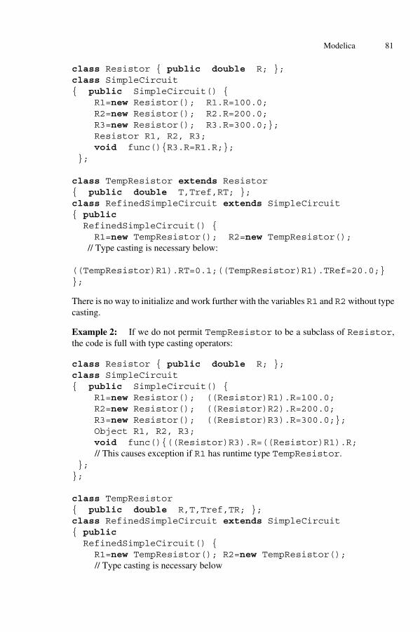
class Resistor { public double R; };class SimpleCircuit{ public SimpleCircuit() { R1=new Resistor(); R1.R=100.0; R2=new Resistor(); R2.R=200.0; R3=new Resistor(); R3.R=300.0;}; Resistor R1, R2, R3; void func(){R3.R=R1.R;};

};

class TempResistor extends Resistor{ public double T,Tref,RT; };class RefinedSimpleCircuit extends SimpleCircuit{ public RefinedSimpleCircuit() { R1=new TempResistor(); R2=new TempResistor();

// Type casting is necessary below:

((TempResistor)R1).RT=0.1;((TempResistor)R1).TRef=20.0;}};

There is no way to initialize and work further with the variables R1 and R2without typecasting.

Example 2: If we do not permit TempResistor to be a subclass of Resistor,the code is full with type casting operators:

class Resistor { public double R; };class SimpleCircuit{ public SimpleCircuit() { R1=new Resistor(); ((Resistor)R1).R=100.0; R2=new Resistor(); ((Resistor)R2).R=200.0; R3=new Resistor(); ((Resistor)R3).R=300.0;}; Object R1, R2, R3; void func(){((Resistor)R3).R=((Resistor)R1).R;

// This causes exception if R1 has runtime type TempResistor. };};

class TempResistor{ public double R,T,Tref,TR; };class RefinedSimpleCircuit extends SimpleCircuit{ public RefinedSimpleCircuit() { R1=new TempResistor(); R2=new TempResistor();

// Type casting is necessary below

81Modelica

((TempResistor)R1).RT=0.1;((TempResistor)R1).TRef=20.0;}};

The class Object is the only mechanism in Java that we can use for construction ofgeneric classes. Since strong type control is enforced in Java, type cast operators arenecessary for every access to R1, R2 and R3. Actually we remove type control fromcompilation time into the run time. This should be discouraged because it makes thecode design more difficult and makes the program error-prone.

To summarize we can reproduce the whole model in Java and build an almost generallibrary. However, many explicit class casting operations make the code difficult andnon-natural.

2.10.3 Final components

The modeler of the SimpleCircuit can state that a component cannot be redeclaredanymore. We declare such component as final.

final Resistor R3(R=300);

It is possible to state that a parameter is frozen to a certain value, i.e. is not a parameteranymore:

Resistor R3(final R=300);

2.10.4 Replaceable classes

To use another resistor model in the class SimpleCircuit, we needed to know thatthere were two replaceable resistors and we needed to know their names. To avoid thisproblem and prepare for replacement of a set of classes, one can define a replaceableclass, ResistorModel. The actual class that will later be used for R1 and R2 musthave Pins p and n and a parameter R in order to be compatible with how R1 and R2are used within SimpleCircuit2. The replaceable model ResistorModel is de-clared to be a Resistor model. This means that it will be enforced that the actualclass will be a subtype of Resistor, i.e., have compatible connectors and parameters.Default for ResistorModel, i.e., when no actual redeclaration is made, is in thiscase Resistor. Note, that R1 and R2 are in this case of class ResistorModel.

class SimpleCircuit2replaceable class ResistorModel = Resistor;

protected ResistorModel R1(R=100), R2(R=200);

final Resistor R3(final R=300);equationconnect(R1.p, R2.p);


connect(R1.p, R3.p);end SimpleCircuit2;

Binding an actual model TempResistor to the replaceable class ResistorModelis done as follows.

class RefinedSimpleCircuit2 = SimpleCircuit2(redeclare class ResistorModel =TempResistor);

This construction is similar to the C++ template construct. ResistorModel canserve as a type parameter. However, in C++ the type parameter cannot have default val-ue. In Modelica the class SimpleCircuit2 is complete and can be used for variableinstantiation. In C++ the class SimpleCircuit2 is a template, which must be instan-tiated first:

template <class ResistorModel>class SimpleCircuit2 {

ResistorModel R1(R=100); ... }

class RefinedSimpleCircuit2 : public SimpleCircuit2<TempResistor> { ... }

3 Implementation issues

3.1 Flattening of equations

Classes, instances and equations are translated into flat set of equations, constants andvariables (see Table 3.1). As an example, we translate the circuit model fromSect. 2.1.

The equation v=p.v-n.v is defined by the class TwoPin. The Resistor classinherits the TwoPin class, including this equation. The circuit class contains avariable R1 of type Resistor. Therefore, we include this equation instantiated for R1as R1.v=R1.p.v-R1.n.v into the set of equations.

The wire labelled 1 is represented in the model as connect(AC.p, R1.p). Thevariables AC.p and R1.p have type Pin. The variable v is a non-flow variablerepresenting voltage potential. Therefore, the equality equation AC.p.v=R1.p.v isgenerated. Equality equations are always generated when non-flow variables areconnected.

Notice that another wire (labelled 4) is attached to the same pin, R1.p. This isrepresented by an additional connect statement: connect(R1.p.R2.p). Thevariable i is declared as a flow-variable. Thus, the equationAC.p.i+R1.p.i+R2.p.i=0 is generated. Zero-sum equations are always

83Modelica

generated when connecting flow variables, corresponding to Kirchhoff’s current law.The complete set of equations generated from the circuit class (see Table 3.1)

consists of 32 differential-algebraic equations. These include 32 variables, as well astime and several parameters and constants.

Table 3.1: Equations generated from the simple circuit model

3.2 Solution and simulation

After flattening, all the equations are sorted. Simplification algorithms can eliminatemany of them. If two syntactically equivalent equations appear only one copy of theequations is kept.

Then they can be converted to assignment statements. If a strongly connected setof equations appears, these can be transformed by a symbolic solver. The symbolicsolver performs a number of algebraic transformations to simplify the dependenciesbetween the variables. It can also solve a system of differential equations if it has asymbolic solution. Finally, C/C++ code is generated, and it is linked with a numericsolver.

The initial values can be taken from the model definition. If necessary, the userspecifies the parameter values (described in Section 2.6)Sect. 2.6. Numeric solvers fordifferential equations (such as LSODE, part of ODEPACK[14]) give the userpossibility to ask about the value of specific variable in a specific time moment. As theresult a function of time, e.g. R2.v(t) can be computed for a time interval [t0, t1] anddisplayed as a graph or saved in a file. This data presentation is the final result of systemsimulation.

AC 0=AC.p.i+Ac.n.iAC.v=Ac.p.v-AC.n.vAC.i=AC.p.iAC.v=AC.VA*sin(2*PI*AC.f*time);

L 0=L.p.i+L.n.iL.v=L.p.v-L.n.vL.i=L.p.iL.v = L.L*L.der(i)

R1 0=R1.p.i+R1.n.iR1.v=R1.p.v-R1.n.vR1.i=R1.p.iR1.v = R1.R*R1.i

G G.p.v = 0

R2 0=R2.p.i+R2.n.iR2.v=R2.p.v-R2.n.vR2.i=R2.p.iR2.v = R2.R*R2.i

wires R1.p.v=AC.p.v // wire 1C.p.v=R1.n.v // wire 2AC.n.v=C.n.v // wire 3R2.p.v=R1.p.v // wire 4L.p.v=R2.n.v // wire 5L.n.v=C.n.v // wire 6G.p.v= AC.n.v // wire 7

C 0=C.p.i+C.n.iC.v=C.p.v-C.n.vC.i=C.p.iC.i = C.C*C.der(v)

flowat

node

0=AC.p.i+R1.p.i+R2.p.i //10=C.n.i+G.i+AC.n.i+L.n.i //20=R1.n.i+ C.p.i // 30 =R2.n.i + L.p.i // 4


In most cases (but not always) the performance of generated simulation code(including the solver) is similar to hand-written C code. Sometimes Modelica is moreefficient than straightforward written C code, because additional opportunities forsymbolic optimization are used.

3.3 Current status

Language definition. As a result from 8 meetings in the period September 1996 -September 1997 the first full definition of Modelica 1.0 was announced in September1997 [23, 29].

Work started in the continuous time domain, since there is a common mathematicalframework in the form of differential-algebraic equations and there are several existingmodeling languages based on similar ideas. There is also significant experience of usingthese languages in various applications. It is expected that the Modelica language willbecome a de-facto standard.

Translators. A translator from a subset of Modelica to Dymola is currently availablefrom Dynasim [8]. We are currently developing another implementation of Modelica.This version of Modelica is integrated with Mathematica [9] similarly to ObjectMath[11,13]. This tool provides both the symbolic processing power of Mathematica, themodeling capability of Modelica, as well as the integrated documentation and program-ming environment offered by Mathematica notebooks. The tool also supports genera-tion of C++ code [10] for high-performance computations.

Graphical model editors. A 2D graphical model editor can be used to define a mod-el by drawing and editing an object diagram very similar to the circuit diagram shownin Fig. 1. Such a model editor is will be implemented for Modelica based on an similarexisting editor for the Dymola language, called Dymodraw. The user can place iconsthat represent the components and connect those components by drawing lines betweentheir iconic representations. For clarity, attributes of the Modelica definition for thegraphical layout of the composition diagram (here: an electric circuit diagram) are notshown in examples. These attributes are usually contained in a Modelica model as an-notations (which are largely ignored by the Modelica translator and used by graphicaltools).

The ObjectMath inheritance graph editor exemplifies another kind of model editor,which supports both display and editing of the inheritance graph. Classes and instancesare represented as graph nodes and inheritance relations are shown as links betweennodes. Such an editor is also planned for Modelica. A partial port of the ObjectMatheditor to Modelica currently exists.

Dynamic simulation visualization. There are currently exist at least two tools fordynamic visualization and animation of Modelica simulations. One of these tools is a3D model viewer called Dymoview [8] for Dymola and Modelica, which displaysdynamic model behavior based on simulations. It can produce realistic visualizations ofmechanical models constructed from graphical objects such as boxes, spheres andcylinders. The visual appearance of a class must be defined together will class

85Modelica

definition. Simultaneously with animation any computed variables can be plotted.Another tool called MAGGIE is described in the next section.

Dynamic computational steering and animation environment. The MAGGIE(Mathematical Graphical Generated Interactive Environment) 3D model visualizer, isbeing developed by us. It supports automatic generation of visual appearance of objects,based on the structure of Modelica models.

Thus, a computational steering environment for the simulation application isautomatically produced from the Modelica model. The user can interactively modifythe structure of the automatically created 3D appearance of the model before start ofvisualization.

However, many parameters of the simulation and geometrical properties of themodel can also be modified during run time, i.e. during simulation and animation. Thisprovides immediate feedback to the user as changing model behavior and visualization.The user can specify the parameters in form-like dialog windows automaticallygenerated based on the Modelica model. For this purpose we reuse our experience withgeneration of such graphical interfaces from C++ and ObjectMath data structures [24].

The simulation code, the interface for parameter control, and a graphical librarybased on the OpenGL toolkit are linked together into a single application which formsa computational steering environment. In contrast to traditional visualization tools thissupports dynamically changing surfaces, that is useful in deformation modeling,hydrodynamics, and volume visualization. By linking all the software components intoa single application we avoid saving large volumes of intermediate results on disk,which improves interactive response of our tool.

Initial experience with MAGGIE is described in [22, 25].

Checking tools. Additional information can be added to improve model consistencyand reliability. One important example is the unit attribute, which provides more in-formation in the user input forms as well as enabling more detailed consistency check-ing as a form of more detailed type checking. For instance, voltage can be defined as

type Voltage = Real(unit="V");

Such a checker can prevent mixing of variables with incompatible units, for examplebelow:

time + position

where both variables have type Real (which are compatible), but have different units– seconds and meters – which are incompatible.

Applications. Several recent papers discussing application of Modelica in differentapplication domains have been written: gear box modeling[15], thermodynamics[16]and mechanics[17].


3.4 Future work

The work by the Modelica Committee on the further development of Modelica andtools will continue. Current issues include definition of Modelica standard libraries.The most recent meeting was in Passau in October 1997, and next one is planned inLinköping in January 1998. Several companies and research institutes are planning de-velopment of tools based on Modelica. In our case, we focus on an interactive imple-mentation of Modelica integrated with Mathematica to provide integration of model de-sign and coding, documentation, simulation and graphics.

Compilation of Modelica. Modelica compilers are developed by us, by Dynasimand planned by other partners. Parser, translator and symbolic solver are developed onthe basis of the experience gained with the Dymola program to convert the model equa-tions into an appropriate form for numerical solvers with target languages C, C++, andJava. Special emphasis will be made on using symbolic techniques for generating effi-cient code for large models.

Parallel simulation. Part of a parallel simulation framework for high performancecomputers earlier developed by PELAB and SKF for bearing applications [26] will beported and adapted for use with Modelica in order to speed up simulation.

Experimentation environment. An integrated experimentation environment is cur-rently being designed and implemented. This integrates simulation, design optimiza-tion, parallelisation, and support documentation in the form of interactive Mathematicanotebooks including Modelica models, live graphics and typeset mathematics.

Library Development. Public domain Modelica component libraries are currentlyunder development by the Modelica design group, for example by DLR in the meca-tronics area, being used in gearbox applications [15]. Several extensions to these librar-ies are needed in order to model complex systems. These libraries will be available foruse in education and in engineering books.

3.5 Conclusion

A new object-oriented language Modelica designed for physical modeling takes somedistinctive features of object-oriented and simulation languages. It offers the user a toolfor expressing non-causal relations in modeled systems. Modelica is able to supportphysically relevant and intuitive model construction in multiple application domains.Non-causal modeling based on equations instead of procedural statements enables ad-equate model design and high level of reusability.

There is a straightforward algorithm translating classes, instances and connectionsinto a flat set of equations. A number of solvers have been attached to the generatedcode for computation of simulation results. The experience shows that Modelica is anadequate tool for design of middle scale physical simulation models.

87Modelica

3.6 Acknowledgments

The Modelica definition has been developed by the Eurosim Modelica technical com-mittee under the leadership of Hilding Elmqvist (Dynasim AB, Lund, Sweden). Thisgroup includes Fabrice Boudaud (Gaz de France), Jan Broenink (University of Twente,The Netherlands), Dag Brück (Dynasim AB, Lund, Sweden), Thilo Ernst (GMD-FIRST, Berlin, Germany), Peter Fritzson (Linköping University, Sweden), AlexandreJeandel (Gaz de France), Kaj Juslin (VTT, Finland), Matthias Klose (Technical Univer-sity of Berlin, Germany), Sven Erik Mattsson (Department of Automatic Control, LundInstitute of Technology, Sweden), Martin Otter (DLR Oberpfaffenhofen, Germany),Per Sahlin (BrisData AB, Stockholm, Sweden), Peter Schwarz (Fraunhofer Institute forIntegrated Circuits, Dresden, Germany), Hubertus Tummescheit (GMD FIRST, Berlin,Germany) and Hans Vangheluwe (Department for Applied Mathematics, Biometricsand Process Control, University of Gent, Belgium). The work by Linköping Universityhas been supported by the Wallenberg foundation as part of the WITAS project.

References

[1] Abadi M., and L. Cardelli: A Theory of Objects. Springer Verlag, ISBN 0-387-94775-2, 1996.

[2] Andersson M.: Object-Oriented Modeling and Simulation of Hybrid Systems.PhD thesis ISRN LUTFD2/TFRT--1043--SE, Department of Automatic Con-trol, Lund Institute of Technology, Lund, Sweden, December 1994.

[3] Barton P.I., and C.C. Pantelides: Modeling of combined discrete/continuousprocesses. AIChE J., 40, pp. 966--979, 1994.

[4] Elmqvist H., D. Brück, and M. Otter: Dymola --- User’s Manual. Dynasim AB,Research Park Ideon,Lund, Sweden, 1996.

[5] Ernst T., S. Jähnichen, and M. Klose: The Architecture of the Smile/M Simula-tion Environment. Proc.15th IMACS World Congress on Scientific Computa-tion, Modelling and Applied Mathematics, Vol. 6, Berlin, Germany, pp. 653-658, 1997

[6] Jeandel A., F. Boudaud., and E. Larivière: ALLAN Simulation release 3.1 de-scription M.DéGIMA.GSA1887. GAZ DE FRANCE, DR, Saint Denis Laplaine, FRANCE, 1997.

[7] Peter Wegner. Concepts and paradigms of object-oriented programming.OOPS Messenger, 1 (1):9-87, August 1990.

[8] Dynasim Home page, http://www.Dynasim.se

[9] Mathematica Home page, http://www.wolfram.com

[10] Fritzson, P. Static and String Typing for Extended Mathematica, Innovation inMathematics, Proceedings of the Second International Mathematica Sympo-sium, Rovaniemi, Finland, 29 June - 4 July, V. Keränen, P. Mitic, A. Hietamäki(Ed.), pp 153-160.


[11] Peter Fritzson, Lars Viklund, Dag Fritzson, Johan Herber. High-Level Mathe-matical Modelling and Programming, IEEE Software, 12(4):77-87, July 1995.

[12] Sahlin P., A. Bring, and E.F. Sowell: The Neutral Model Format for buildingsimulation, Version 3.02. Technical Report, Department of Building Sciences,The Royal Institute of Technology, Stockholm, Sweden, June 1996.

[13] ObjectMath Home Page, http://www.ida.liu.se/labs/pelab/omath

[14] Hindmarsh, A.C., ODEPACK, A Systematized Collection of ODE Solvers,Scientific Computing, R. S. Stepleman et al. (eds.), North-Holland, Amster-dam, 1983 (Vol. 1 of IMACS Transactions on Scientific Computation), pp. 55-64, also http://www.netlib.org/odepack/index.html

[15] Otter M., C. Schlegel, and H. Elmqvist, Modeling and Real-time Simulation ofan Automatic Gearbox using Modelica. In Proceedings of ESS'97 - EuropeanSimulation Symposium, Passau, Oct. 19-23, 1997.

[16] Tummescheit H., T. Ernst and M. Klose, Modelica and Smile - A Case StudyApplying Object-Oriented Concepts to Multi-facet Modeling. In Proceedingsof ESS'97 - European Simulation Symposium, Passau, Oct. 19-23, 1997.

[17] Broenink J.F., Bond-Graph Modeling in Modelica. In Proceedings of ESS’97- European Simulation Symposium, Passau, Oct. 19-23, 1997.

[18] SIMULINK 2 - Dynamic System Simulation. http://www.math-works.com/ products/simulink/

[19] ACSL software. http://www.mga.com

[20] Jan Van der Spiegel. SPICE - A Brief Overview. http://howard.engr.siu.edu/elec/faculty/etienne/spice.overview.html, http://www.seas.upenn.edu/~jan/spice/spice.overview.html

[21] ADAMS - virtual prototyping virtually anything that moves. http://www.adams.com

[22] V. Engelson, P. Fritzson, D. Fritzson. Generating Efficient 3D graphics anima-tion code with OpenGL from object oriented models in Mathematica, In Inno-vation in Mathematics. Proceedings of the Second International MathematicaSymposium, Rovaniemi, Finland, 29 June - 4 July 1997, V.Keränen, P. Mitic,A. Hietamäki (Ed.), pp. 129 - 136

[23] Modelica Home Page http://www.Dynasim.se/Modelica

[24] V. Engelson, P. Fritzson, D. Fritzson. Automatic Generation of User InterfacesFrom Data Structure Specifications and Object-Oriented Application Models.In Proceedings of European Conference on Object-Oriented Programming(ECOOP96), Linz, Austria, 8-12 July 1996, vol. 1098 of Lecture Notes inComputer Science, Pierre Cointe (Ed.), pp. 114-141. Springer-Verlag, 1996

[25] V. Engelson, P. Fritzson, D. Fritzson. Using the Mathematica environment for

89Modelica

generating efficient 3D graphics. In Proceedings of COMPUGRAPHICS/EDUGRAPHICS, Vilamoura, Portugal, 15-18 December 1997 (to appear).

[26] D. Fritzson, P. Nordling. Solving Ordinary Differential Equations on ParallelComputers Applied to Dynamic Rolling Bearing Simulation. In Parallel Pro-gramming and Applications, P. Fritzson, L. Finmo, eds., IOS Press, 1995

[27] SIMPACK Home page http://www.cis.ufl.edu/mpack/~fish-wick/simpack.html

[28] M. Löfgren, J. Lindskov Knudsen, B. Magnusson, O. Lehrmann Madsen Ob-ject-Oriented Environments - The Mjølner Approach ISBN 0-13-009291-6,Prentice Hall, 1994. See also Beta Home Page, http://www.dai-mi.aau.dk/~beta/

[29] H. Elmqvist, S. E. Mattsson: “Modelica - The Next Generation ModelingLanguage - An International Design Effort”. In Proceedings of First WorldCongress of System Simulation, Singapore, September 1-3 1997.


Modelica - A Uniﬁed Object-Oriented Language for System Modeling · PDF file ·...

Documents

Transcript of Modelica - A Uniﬁed Object-Oriented Language for System Modeling · PDF file ·...