Modèles de files d'attente pour l'analyse des stratégies ... · Remerciement A l’issue de la...
131
HAL Id: tel-01478614 https://tel.archives-ouvertes.fr/tel-01478614 Submitted on 28 Feb 2017 HAL is a multi-disciplinary open access archive for the deposit and dissemination of sci- entific research documents, whether they are pub- lished or not. The documents may come from teaching and research institutions in France or abroad, or from public or private research centers. L’archive ouverte pluridisciplinaire HAL, est destinée au dépôt et à la diffusion de documents scientifiques de niveau recherche, publiés ou non, émanant des établissements d’enseignement et de recherche français ou étrangers, des laboratoires publics ou privés. Modèles de files d’attente pour l’analyse des stratégies de collaboration dans les systèmes de services Jing Peng To cite this version: Jing Peng. Modèles de files d’attente pour l’analyse des stratégies de collaboration dans les systèmes de services. Autre. Université Paris-Saclay, 2016. Français. <NNT: 2016SACLC089>. <tel-01478614>
Transcript of Modèles de files d'attente pour l'analyse des stratégies ... · Remerciement A l’issue de la...

HAL Id: tel-01478614https://tel.archives-ouvertes.fr/tel-01478614
Submitted on 28 Feb 2017
HAL is a multi-disciplinary open accessarchive for the deposit and dissemination of sci-entific research documents, whether they are pub-lished or not. The documents may come fromteaching and research institutions in France orabroad, or from public or private research centers.
L’archive ouverte pluridisciplinaire HAL, estdestinée au dépôt et à la diffusion de documentsscientifiques de niveau recherche, publiés ou non,émanant des établissements d’enseignement et derecherche français ou étrangers, des laboratoirespublics ou privés.
Modèles de files d’attente pour l’analyse des stratégiesde collaboration dans les systèmes de services
Jing Peng
To cite this version:Jing Peng. Modèles de files d’attente pour l’analyse des stratégies de collaboration dans les systèmes deservices. Autre. Université Paris-Saclay, 2016. Français. <NNT : 2016SACLC089>. <tel-01478614>


Remerciement
A l’issue de la rédaction de cette recherche, je n’aurais jamais pu réaliser ce travail doc-
toral sans le soutien d’un grand nombre de personnes: l’équipe encadrante de thèse,
mes amis, mes collègues et mes parents.
Premièrement, je tiens à remercier mon directeur de thèse, monsieur Yves DALLERY,
pour la confiance qu’il m’a accordée en acceptant de diriger ce travail doctoral. Je
voudrais remercier sincèrement mes encadrants, monsieur Oualid JOUINI et monsieur
Zied JEMAI, pour leurs multiples conseils et toutes les heures quils ont consacrées à en-
cadrer cette recherche.
Mes remerciements vont également à monsieur Marc AIGUIER, monsieur Jean-Philippe
GAYON, monsieur Yacine REKIK, et monsieur Fabrice CHAUVET pour avoir accepté de
participer à ce jury de thèse, pour avoir bien voulu porter à mon travail, pour l’occasion
de discuter du résultat de mes recherches et les recherches possibles en perspective avec
eux et pour tous les conseils intéressants sur mon travail.
Je voudrai remercier le China Scholarship Council qui a financé cette thèse.
Mes remerciements vont aussi à mes amis et mes collègues du laboratoire qui avec cette
question récurrente ≪ quand est-ce que tu la soutiens cette thèse? ≫, m’ont permis de
ne jamais dévier de mon objectif final. Merci à Delphine et Corinne pour tous les aides
pendant le processus de soutenance. Je remercie également tous les participants de ma
iii

soutenance de thèse pour leurs présences à la date spécifique avant Noël.
Ma reconnaissance va à ceux qui ont plus particulièrement assuré le soutien affectif de
ce travail doctoral : ma famille. Ma mère m’encourage énormément quand j’ai rencontré
la crise la plus importante pendant la thèse. Je souhaite enfin remercier particulièremen-
t mes amis qui m’ont accompagné et m’ont aidé beaucoup pendant ma vie doctorale,
Wenjing, Shanshan, Huan, Xue et Shouyu, malgré certaines ont déjà rentrés en Chine.
Jing PENG
iv

Contents
Introduction 5
1.1 Background & motivation . . . . . . . . . . . . . . . . . . . . . . . . . . . . . 6
1.2 Objective & contributions . . . . . . . . . . . . . . . . . . . . . . . . . . . . . 9
1.3 Thesis structure . . . . . . . . . . . . . . . . . . . . . . . . . . . . . . . . . . . 11
Cooperation with General Service Times 13
2.1 Introduction . . . . . . . . . . . . . . . . . . . . . . . . . . . . . . . . . . . . . 15
2.2 Literature review . . . . . . . . . . . . . . . . . . . . . . . . . . . . . . . . . . 16
2.3 Service pooling modeling with general service times . . . . . . . . . . . . . 18
2.4 Service pooling with a fixed capacity . . . . . . . . . . . . . . . . . . . . . . 21
2.4.1 Non-emptiness of the core . . . . . . . . . . . . . . . . . . . . . . . . 22
2.4.2 Cost allocation rules . . . . . . . . . . . . . . . . . . . . . . . . . . . . 27
2.4.3 Numerical results and analysis . . . . . . . . . . . . . . . . . . . . . . 30
2.5 Service pooling with the optimized capacity . . . . . . . . . . . . . . . . . . 34
2.5.1 Optimal service rate in M/GI/1 systems . . . . . . . . . . . . . . . . 34
2.5.2 Service pooling game with optimized service capacity . . . . . . . . 37
2.5.3 Cost allocation rules for the service pooling game (N, Copt) . . . . . 40
2.5.4 Comparison between φp,λ and shopt . . . . . . . . . . . . . . . . . . . 43
2.6 Conclusion . . . . . . . . . . . . . . . . . . . . . . . . . . . . . . . . . . . . . . 47
1

Collaboration with Impatient Customers 51
3.1 Introduction . . . . . . . . . . . . . . . . . . . . . . . . . . . . . . . . . . . . . 53
3.2 Modeling and observations . . . . . . . . . . . . . . . . . . . . . . . . . . . . 55
3.2.1 Service systems modeling with impatience . . . . . . . . . . . . . . . 55
3.2.2 Observation of queue length and abandonment probability . . . . . 57
3.3 Collaboration under a fixed service capacity . . . . . . . . . . . . . . . . . . 59
3.3.1 Non-emptiness of the core of the game (N, C f ix) . . . . . . . . . . . 60
3.3.2 Impact of abandonment on the stability of the Shapley value . . . . 63
3.4 Collaboration under the optimized service capacity . . . . . . . . . . . . . . 67
3.5 Conclusion . . . . . . . . . . . . . . . . . . . . . . . . . . . . . . . . . . . . . . 70
Collaboration for Multi-server Service Systems 71
4.1 Introduction . . . . . . . . . . . . . . . . . . . . . . . . . . . . . . . . . . . . . 73
4.2 Models and preliminary study . . . . . . . . . . . . . . . . . . . . . . . . . . 74
4.2.1 Service pooling modeling . . . . . . . . . . . . . . . . . . . . . . . . . 74
4.2.2 Performance comparison . . . . . . . . . . . . . . . . . . . . . . . . . 77
4.3 Service pooling games . . . . . . . . . . . . . . . . . . . . . . . . . . . . . . . 79
4.3.1 Service pooling games with exponential services . . . . . . . . . . . 80
4.3.2 Comparison of costs in (N, Cs) and (N, Cm) . . . . . . . . . . . . . . 80
4.4 Numerical examples . . . . . . . . . . . . . . . . . . . . . . . . . . . . . . . . 81
4.4.1 Impact of customer arrival rates λi . . . . . . . . . . . . . . . . . . . . 82
4.4.2 Impact of customer abandonment θ . . . . . . . . . . . . . . . . . . . 87
4.4.3 Impact of service times variability cv . . . . . . . . . . . . . . . . . . 88
4.5 Pooling in multi-class service systems . . . . . . . . . . . . . . . . . . . . . . 88
4.6 Conclusion . . . . . . . . . . . . . . . . . . . . . . . . . . . . . . . . . . . . . . 91
Conclusion and Perspectives 93
2

CONTENTS
Appendix 97
Appendix of Chapter 2 . . . . . . . . . . . . . . . . . . . . . . . . . . . . . . . . . . 97
Appendix A . . . . . . . . . . . . . . . . . . . . . . . . . . . . . . . . . . . . . 97
Appendix of Chapter 3 . . . . . . . . . . . . . . . . . . . . . . . . . . . . . . . . . . 101
Appendix B . . . . . . . . . . . . . . . . . . . . . . . . . . . . . . . . . . . . . 101
Appendix C . . . . . . . . . . . . . . . . . . . . . . . . . . . . . . . . . . . . . 102
Appendix D Résumé étendu . . . . . . . . . . . . . . . . . . . . . . . . . . . . . 109
Bibliography 115
3

CONTENTS
4

Chapter 1
Introduction
This chapter provides a general introduction to this Ph.D. thesis. It is divided
into three main sections. First, we present the background and the motivations
of our work. Second, we highlight our objective and contributions. Finally, we
describe the structure of the manuscript.
5

CHAPTER 1. INTRODUCTION
1.1. Background & motivation
Many of our daily activities depend on services and service providers, from the e-mail
we check in the early morning to the public transportation service we take to our work-
ing place, from the restaurant we eat in at noon to the package we receive during the day.
Services are everywhere in our life, including finance (banking, stocks), health (person-
al physician, hospital), communication (e-mail, 4G network), public services (electricity,
police), etc. [Daskin, 2010]
In past twenty years, the service sector has emerged as the primary sector in the
world economy (Figure 1.1), especially in developed countries. Based on the report
from the office of the United States Trade Representative, for instance, four out of five
jobs in the U.S. are provided by service industry [USTR, 2014]. Furthermore, service
sector accounted for 78.76% gross domestic product (GDP) in France 2015 according to
statistical data from the World Bank group.
Figure 1.1: Growth of the service sector in world GDP
In the context of economic globalization, competition and cooperation in service
industries have become more and more popular: price competition among fast food
6

1.1. BACKGROUND & MOTIVATION
restaurant chains, combination operation of telecommunication companies, collabora-
tive after-sales and maintenance services in electronic manufacturing industry, just to
name a few. In this thesis, we study collaborative strategies in homogeneous service
systems. We focus in particular on resource pooling strategies. Our approach consists
of using queueing modeling for service systems and game theory for the analysis of
interactions between service providers. In what follows, we briefly discuss collaboration
strategies and resource pooling.
Collaboration strategies in services
In order to improve the system performance or reduce expenses, there are several ba-
sic cooperative methods: queueing cooperation, e.g., scheduling among simultaneous
arrival agencies or rerouting among different servers [Katta and Sethuraman, 2006, Kay-
i and Ramaekers, 2010]; service pooling, e.g., service rate pooling or staffing alloca-
tion [Guo et al., 2013]; cross-training [Tekin et al., 2014]; collaboration with third-party
service providers, e.g., service outsourcing [Aksin et al., 2008], etc. It is sometimes useful
to combine these methods to form a more profitable collaborative structure [Anily and
Haviv, 2014].
Cooperation methods can be classified broadly into three typical forms (Figure 1.2):
vertical form, the collaboration between customers and servers, e.g. phone packages
signed with telecommunication companies, fitness cards brought from gyms; horizontal
form, the collaboration among homogeneous servers, e.g. after-sale services of electronic
products of different brands; and external form, the collaboration with another party out
of the service systems, e.g., customer services outsourcing abroad.
Among majority efficiencies brought by service collaborations, cost reduction is the
most marked driver for service providers. The service capacity cost and the waiting
cost in the queue/system are widely used in the literature [Anily and Haviv, 2010, Özen
et al., 2011, Karsten et al., 2015b, Yu et al., 2015].
7

CHAPTER 1. INTRODUCTION
Figure 1.2: Service cooperation classification
Resource pooling
From first study in [Stidham, 1970], pooling for queueing systems has been widely in-
vestigated in the literature on the design of service systems. It is well known that the
service capacity pooling naturally leads to economies of scale in stochastic flows in op-
eration management studies [Smith and Whitt, 1981, Bell and Williams, 2005]. This
operational efficiency improvement occurs in the disappearance of idle service resources
in the presence of congestion in queues. It is both valid within some departments of
an economic entity, e.g., reservation pooling in a restaurant [Thompson and Kwortnik,
2008], or among multiple independent entities [González and Herrero, 2004, Garcia-Sanz
et al., 2008, Anily and Haviv, 2010, Kayi and Ramaekers, 2010, Tekin et al., 2014, Anily
and Haviv, 2014].
Applications in practice for service pooling among homogeneous service providers
are numerous. For instance, different departments in a hospital could share a common
operating theatre and afford the joint expenses. Different hospital departments could
also share a joint service capacity in terms of beds in a common ward, which would
alleviate congestion. Another example is in the context of after-sales for new categories
of electronic products. Such products are likely to have low after-sales demand rates for
each retailer individually. The retailers could therefore provide together a joint after-
sales service to reduce service start-up costs and also improve service quality. For avi-
ation services, the joint check-in service for different airline companies is an additional
8

1.2. OBJECTIVE & CONTRIBUTIONS
example for service pooling applications.
Prior to services, resource pooling in supply chains has already attracted a lot of at-
tention. The first contribution to gains splitting is considered in a multistore economic
order quantity with safety stock in [Gerchak and Gupta, 1991]. Later, [Hartman and
Dror, 1996] and [Özen et al., 2008] extend this problem in a cooperative game environ-
ment. The cooperation costs sharing issue in the multi-retailer newsvendor problem is
first considered by [Hartman et al., 2000] and [Müller et al., 2002]. Relative problem are
also fruitfully studied in the joint replenishment problem [Meca et al., 2004, Anily and
Haviv, 2007, Zhang, 2009, Elomri et al., 2012] and the economic lot-sizing model [Van den
Heuvel et al., 2007, Guardiola et al., 2009].
There are similarities between service and manufacturing operations, which are both
concerned with the efficiency, effectiveness, quality problems, and motivated by the
cost reduction. In contrast to the research in the manufacturing industry, the relative
research in service industry could not meet requirements of its enormous economic
share. Services are mainly characterized by complex operations and a high impact of
human factors. In this thesis, we account for these two aspects through the analysis of
the impact of service duration variability and customer abandonment, respectively. We
study the problem where independent service providers could be subject to cooperate
with each other. We consider the resource pooling strategy in different service systems
and provide corresponding pooling strategies using cooperative game theory.
1.2. Objective & contributions
The objective of this thesis is to study the impact of the features of service variability
and customer abandonment on collaboration strategies. Motivated by cost reduction,
we tackle the resource pooling problem between independent service providers. We use
a queueing approach for the modeling of these features. More concretely, we address
the two following questions: 1) which coalition strategy should be used? and 2) which
allocation rule should be selected in order to maintain the stability of the coalition? We
9

CHAPTER 1. INTRODUCTION
use cooperative game theory, which provides interesting concepts to analyze profitable
coalition structures and solve the cost-sharing problem among the participants.
The main contributions of this thesis can be summarized as follows.
First, we study the cost-sharing problem among independent service providers in a
service capacity pooling system with general service times. The effective improvemen-
t is achieved by reducing the resource idleness in case of congestion. We model both
the service provider and the cooperative coalition as single server queues with general
service times. For the two situations of pooling with a fixed service capacity and pool-
ing with the optimized service capacity, we define the corresponding cooperative games
and analyze the core allocations. For the fixed capacity case, we prove that the core is
non-empty. The characteristic function is neither concave nor monotone in the afore-
mentioned game. However, we prove that the service pooling game with the optimized
service capacity is concave. For this concave game, we find two stable allocation rules
and illustrate a combined cost allocation strategy.
Second, we consider a group of homogeneous and independent single server service
providers with impatience, where a customer quits the system without service whenev-
er her waiting time in the queue exceeds his patience time threshold. The advantage of
collaboration in the service systems accounting customer abandonment, is not only the
sharing of instant idle resources but also the reducing of abandoned customers. Under
Markovian assumptions for inter-arrival, service and patience times, we define a coop-
erative game with transferable utility and a fixed service capacity for each coalition. We
prove that the grand coalition is the most profitable coalition and that the game has a
non-empty core. We then examine the impact of abandonment on the stability of Shapley
value. Furthermore, we prove the concavity of the waiting queue length with respect to
the abandonment rate, and give a condition under which the Shapley value is situated in
the core. We also study the cost-sharing problem of the relative cooperative game with
the optimized service capacity, and prove that the proportional allocation rule based on
customer arrival rates gives a dynamic stable allocation to all relative sub-games.
In the previous studies, we use the ’super-server’ assumptions. The main reason
10

1.3. THESIS STRUCTURE
for this assumption is that dealing with multi-server queues with general service times
and customer abandonment is very hard. To assess the quality of this assumptions, we
address the service pooling problem in the multi-server pooling setting. Although it is
intuitive to expect efficiency improvements in the pooled multi-server system, it is not
obvious to conclude that all members will benefit from pooling as it is the case for the
’super-server’. We compare between two pooling settings from a coalition perspective.
We numerically evaluate the effects of service variability and customer abandonment on
the two corresponding games.
1.3. Thesis structure
The remaining part of this Ph.D dissertation contains four chapters.
In Chapter 2, we study the cost-sharing problem in service systems with general
service times. The paper version of this chapter is under the second round review in
Naval Research Logistics [Peng et al., a]. Secondly, we analyze cooperative strategies in
the presence of customer abandonment in Chapter 3. The paper version of this chapter
is submitted to IIE Transactions [Peng et al., b]. In Chapter 4, we compare between
’super-server’ and multi-server modeling in terms of stability and cost allocations. The
paper version of this chapter is a working paper to be submitted for publication. Finally,
Chapter 5 is devoted to general conclusions and perspectives. Figure 1.3 provides a
general overview of the dissertation content.
11

CHAPTER 1. INTRODUCTION
Figure 1.3: Dissertation structure
12

Chapter 2
Cooperation in Service Systems with Gen-
eral Service Times
In this chapter, we study the cost-sharing problem among independent service
providers in a service capacity pooling system with general service times. The
effective improvement is achieved by reducing the resource idleness in case of
congestion. We model both the service provider and the cooperative coalition
as single server queues with general service times, and attempt to answer the
following questions: 1) which coalition strategy should be used; and 2) which
allocation rule should be selected in order to maintain the stability of the coali-
tion?
For both situations, (a) pooling with a fixed service capacity and (b) pooling with
the optimized service capacity, we define the corresponding cooperative game
and analyze the core allocations. For the fixed capacity case, we prove that the
core is non-empty. The characteristic function is not concave and monotone in
13

CHAPTER 2. COOPERATION WITH GENERAL SERVICE TIMES
the aforementioned game. However, we prove that the service pooling game
with the optimized service capacity is concave. For this concave game, as it is
widely admitted, the Shapley value provides a core allocation rule. We prove
that the proportional allocation rule based on the individual customer arrival
rates, is also located in the core. Moreover, we show that the allocation scheme
evolved is a Population Monotonic Allocation Scheme (PMAS) for this game.
We finally analytically compare between the performance of the Shapley value
and the proportional rule in terms of the individual profits from the cooperation,
and illustrate a combined allocation strategy.
14

2.1. INTRODUCTION
2.1. Introduction
The obvious profit of service pooling is the congestion mitigation in the whole system,
owing to the reduction of idleness with the presence of waiting customers. The pooling
advantage for the entire alliance is apparent, but the collective interests cannot be the
incentive for each individual service provider to join the coalition. It is therefore impor-
tant to address the following questions: which service providers should cooperate; and
how to share the pooling cost among the participants to keep each individual and subset
staying in the coalition?
Motivated by real-life applications, we consider in this chapter a set of independent s-
ingle server service providers, each of which faces its own incoming stream of customers.
Customer inter-arrival and service times are assumed to be random and independently
distributed. We suppose that every incoming stream is strictly unrelated to those of oth-
er providers. This means that there is no competition in the set. Service providers could
then join a profitable coalition by operating their service capacities in common. Alterna-
tively, each provider makes his own decision independently to either join any coalition
or not, based on his individual benefit. Once the coalition is formed, the most interesting
problem for every unit in the entire coalition becomes a cost-sharing problem.
Cooperative game theory provides interesting concepts to look for profitable coali-
tion structures and solve the cost-sharing problem among the participants. We assume
here that the total cost is a transferable utility, e.g., money in the general case. The
corresponding cooperative game with transferable utility (TU-game) is defined among
a set of independent service providers, and has a characteristic function defined by the
operating coalition costs. We prove that the service pooling game with fixed service
capacity sharing always has a stable cost-sharing solution for the grand coalition. Stable
cost-sharing means that all subsets pay less in the grand coalition than in each individual
setting. We also observe that the higher is the variability of service times, the larger is
the relative revenue to the cooperative coalition. Under optimized service capacity con-
ditions, we prove that the corresponding service pooling game is concave. We consider
15

CHAPTER 2. COOPERATION WITH GENERAL SERVICE TIMES
two stable cost allocation rules for this game: the proportional allocation rule depending
on customer arrival rates and the Shapley value, and discuss their fairness using the
benefit ordering property.
The rest of this chapter is structured as follows. We briefly review the relevant lit-
erature in the next section. In Section 2.3, we present the individual and collaborative
modeling of service systems. In Section 2.4, we define and analyze the service pooling
problem with a fixed service capacity as a TU-game. Then, we consider the optimal
service rate and analyze the corresponding service pooling game in Section 2.5. We con-
sider two stable allocation rules for this game and provide some analytical discussions
of the results.
2.2. Literature review
Our work is related to the stream of literature dealing with the study of the benefits
of resource pooling. In the early research [Stidham, 1970], the optimal design of single
server systems is studied for different service cost functions. Moreover, the resource
pooling as a parallel-server system is applied in the heavy transportation case in [Har-
rison and López, 1999]. In [Wallace and Whitt, 2004], the authors consider both the
resource pooling and staffing in a particular call center application. While focusing on
the profitability, [Dijk and Sluis, 2008, Jouini et al., 2008] discuss the benefit of pooled
and unpooled scenarios in call centers. For an inventory application, the sensitivity of
the inventory pooling benefit is investigated and evaluated by comparing several forms
of capacity pooling in [Benjaafar et al., 2005].
This work is also related to the large body of literature focusing on the cooperative
behavior among independent participants using cooperative game theory. [González and
Herrero, 2004] is the earliest research that deals with the cost-sharing problem for an op-
erating theatre in medical service. The authors separate the operating theatre costs as
variable and fixed costs, and focus on the Shapley value of two sub-games. In [Garcia-
Sanz et al., 2008], the authors extend the work in [González and Herrero, 2004] by con-
16

2.2. LITERATURE REVIEW
sidering preemptive priority for the customers from different individual servers, which
allows to provide a more profitable pooling system. Our work is clearly related to two
recent papers [Yu et al., 2015, Anily and Haviv, 2010] that consider M/M/1 modeling
to study the service capacity pooling problem using cooperative game theory. [Yu et al.,
2015] uses the optimal service rate that minimizes the system operating costs, and an
incomplete information problem is also treated. In [Anily and Haviv, 2010], the authors
choose a service rate varying with the customer incoming rate. In [Karsten et al., 2015b]
and [Karsten et al., 2011], the service collaboration problems in [Yu et al., 2015] and [Ani-
ly and Haviv, 2010] are extended to multi-server settings using Erlang-C and Erlang-B
queueing models, respectively. Similar to [Karsten et al., 2015b, Karsten et al., 2011], we
consider here a single server modeling. Yet, the cost structure is different since we focus
on the cost of the waiting time in the queue instead of that in the system. This makes the
results different. For instance, the concavity of the auxiliary game provided in [Anily
and Haviv, 2010] is not compatible with our setting. More importantly, we allow service
time to be generally distributed. Despite its prevalence in practice, no existing studies
allow for non-Markovian service times.
The cost allocation problem of service capacity pooling is a challenging subject. The
objective is to find the stable cost allocations, which means that no coalition has an
incentive to split off. In cooperative games, the core defined in [Gillies, 1959], presents
the set of all stable cost allocations. For service pooling games, the Shapley value as
an accepted fair cost allocation rule is discussed in [González and Herrero, 2004, Anily
and Haviv, 2010]. Note also that the proportional allocation rule could be used as a
general cost-sharing rule for this kind of problems. It depends on the structure of the
game characteristic function [Garcia-Sanz et al., 2008, Yu et al., 2015, Karsten et al.,
2015b, Karsten et al., 2011]. In [Anily and Haviv, 2010], the authors divide all stable
allocations into two families: non-negative and negative ones, and propose an algorithm
to generate all stable allocations. A corrected proportional allocation rule is given in [Yu
et al., 2015] to handle the eventual incomplete information problem. For our game
with the optimized service capacity, we find two stable allocation rules. Considering the
17

CHAPTER 2. COOPERATION WITH GENERAL SERVICE TIMES
complexity and the fairness of the two rules, we discuss their use under different setting.
There are also several papers focusing on other service collaboration issues using co-
operative game theory: [Katta and Sethuraman, 2006] considers a scheduling problem
in a service facility under a rush hour regime. They propose two solution concepts,
Random Priority and Constrained Random Priority cores, if monetary compensation
are allowed. For a similar scheduling problem, the only cost allocation rule satisfying
Pareto-efficiency, anonymity and strong strategy-proofness, is proved by [Kayi and Ra-
maekers, 2010]. In [Mishra and Rangarajan, 2007], the authors characterize the Shapley
value solution for a job scheduling problem. These kind of problems are referred to as
queueing problems in [Chun, 2006b, Chun, 2006a]. [Guo et al., 2013] studies the staffing
problem in call centers, where a square-root safety staffing rule is selected to define the
number of agents required for each coalition in the system. They show that the Shapley
value is a fair staff allocation rule in the core of the square-root safety staffing game.
In addition to services, cooperation in supply chains has been already a fruitful re-
search subject to make joint pricing and inventory decisions. In order to improve oper-
ations and reactivity to the market changes, working with outside partners is more and
more important for supply chain actors over the past decades [Zhang, 2009, Dror et al.,
2012, Elomri et al., 2012, Timmer et al., 2013]. There are numerous examples for cooper-
ation cases: collaborative forest transportation [Fiestras-Janeiro et al., 2013], cooperative
procurement [Drechsel and Kimms, 2010], shipping pooling of automobiles [Sherali and
Lunday, 2011], lateral transshipments pooling [Satir et al., 2012], just to name a few.
A interesting review of the application of both cooperative and non-cooperative game
theories in supply chain is provided by [Nagarajan and Sošic, 2008].
2.3. Service pooling modeling with general service times
We consider a set of n service providers, N = {1, . . . , n}. Each service provider i ∈ N
is modeled as a single server queue handling a single class of customers. We assume
that the waiting space is large enough, no customer would abandon after arriving at
18

2.3. SERVICE POOLING MODELING WITH GENERAL SERVICE TIMES
the system, and there is no failure in service processing, i.e., no retrial is considered
here. The incoming stream of customers to service provider i ∈ N follows a Poisson
process, and customers are served in the order of their arrivals, i.e., under the first come,
first served (FCFS) discipline of service. Service times for a given service provider are
assumed to be i.i.d. and allowed to follow a general distribution. Following the above
assumptions, the individual service process is modeled as an M/GI/1 queueing system.
For the total operating cost, we consider a traditional economic framework with two
types of costs [Guajardo and Rönnqvist, 2015]. The first type is a linear capacity cost
per unit time, which is proportional to system service capacity. This may capture the
equipment’s depreciation or maintenance fee, employee’s salary, etc. We also assume a
congestion cost incurred for each unit of time the customers spend in the queue. For
each service provider i, we define the following parameters:
• λi: Mean arrival rate of customers to provider i;
• Ti: A random variable describing the service time at server i, with mean 1/µi and
coefficient of variation cvi;
• ρi = λi/µi: Server utilization for provider i, with µi > λi;
• Wq,i: Customer expected waiting time in the queue for provider i;
• ch,i: Service capacity cost parameter per unit time per service capacity for provider
i;
• cw,i: Congestion cost parameter per unit time per customer waiting in the queue at
server i.
For service provider i, we denote the capacity, the congestion and the total operating
costs per unit time by Ch,i, Cw,i and Ci, respectively. Using the Pollaczek-Khinchine formula
in [Pollaczeck, 1930], we may write
Ci = Ch,i + Cw,i = ch,iµi + cw,iλiWq,i = ch,iµi + cw,iλiλiE(T2
i )
2(1 − ρi). (2.1)
The service capacity pooling consists of two typical methods with pooling demand.
In the first one, the service providers form a common facility with parallel-servers and
one single queue, which will be considered in Chapter 4. In the second one, the servers
19

CHAPTER 2. COOPERATION WITH GENERAL SERVICE TIMES
share their service capacities together and work as a ’super-server’, i.e., a single serv-
er system with a high service capacity. As in [Yu et al., 2015] and [Anily and Haviv,
2010], we consider here the second configuration. We assume that u independent ser-
vice providers of any subset ∅ ⊂ U = {1, . . . , u} ⊆ N would decide to share their
capacities as a ’super-server’. Individual arrival processes are assumed to be indepen-
dent. Therefore, the combined arrival process, at a rate of λU = ∑U λi follows a Poisson
process. We assume that the pooling system provides same services in terms of speed
and quality (compared to the case of individual providers), and service times are also
i.i.d.. We denote the mean service capacity by µU for the pooling system U. Based on
these assumptions, the u providers act as an M/GI/1 ’super-server’ system (Figure 2.1).
Figure 2.1: Individual and coalition service systems
The service providers, which provide the same service and have similar scales, are
assumed to also have similar service capacity expenses. This could be justified by the use
of the same technology and the similarity of the staff salary expenses. We then assume
for simplicity that the service capacity cost parameters to be the same, ch,i = ch, and
the coefficients of variation of service times to be identical, cvU,i = cvU = cvN, for all
providers in the set N. We only consider a single class of customers in the pooling sys-
tem. The congestion parameters are assumed to be identical, cw,i = cw, for all customers
from all service servers. The service providers are also all assumed to be risk-neutral.
The total cost of the pooling system U ⊂ N, is the sum of service capacity cost and
system congestion cost. For a pooling system U, we define the parameters as follows:
• λU: Mean arrival rate of customers for the pooling system U;
• TU: A random variable, service time at the pooling server U, with mean 1/µU and
20

2.4. SERVICE POOLING WITH A FIXED CAPACITY
coefficient of variation cvU;
• ρU = λU/µU: Server utilization for the pooling system U, with µU > λU;
• Wq,U: Customer expected waiting time in the queue for the pooling system U;
• ch: Service capacity cost parameter per unit time per service capacity for any subset
of N;
• cw: Congestion cost parameter per unit time per customer waiting in the queue for
any subset of N.
For a pooling system U, we denote the capacity, the congestion and the total operat-
ing costs per unit time by Ch,U, Cw,U and CU, respectively. The expected total cost per
unit time is given by
CU = Ch,U + Cw,U = chµU + cwλUWq,S = chµU + cwλUλUE(T2
U)
2(1 − ρU). (2.2)
With the above notations and definitions, we propose both the individual service
model and the pooling service model using an M/GI/1 queueing modeling. Our objec-
tive is to investigate the profitability and stability of service capacity pooling. It consists
of two steps: (i) confirm that the service capacity pooling is profitable for the whole set
and for each provider; (ii) verify that the coalition structure could be stable under some
cost allocations. Cooperative game theory provides a framework to formulate, structure
and analyze the cooperative behavior of independent individuals in collaboration. In the
two following sections, we construct TU-games under two different conditions: (i) each
provider has a fixed individual service capacity and the capacities remain fixed in any
coalition; (ii) the service capacity for any individual/pooling server could be optimized.
2.4. Service pooling game with fixed service capacity
In this section, we assume that the service capacity of every individual service provider
is fixed. This corresponds to situations where the changing of equipments or the physical
location is too expensive or almost impossible. We thus consider the pooling capacity
µU of any subset U as the sum of the service capacities of its members. Let us denote by
21

CHAPTER 2. COOPERATION WITH GENERAL SERVICE TIMES
C f ix(·) the total cost function of a subset U ⊂ N. We have
C f ix(∅) = 0, C f ix(U) = CU(λU, µU = ∑j∈U
µj), for any ∅ ⊆ U ⊆ N. (2.3)
Consider a finite set of independent service providers N = {1, . . . , n} (a set of play-
ers), which is known as the grand coalition in cooperative game. Let U be any subset
of N, which is called a coalition (a subset of players). In every coalition, the players
could reduce the total costs by service pooling. We assume that each service provider
could only join one coalition, and the pooling cost could be redistributed among the
providers with no limitation. Thus, a TU-game (N, C f ix) is completely specified by its
characteristic function C f ix : 2N → R defined for any sub-coalition of N.
To simplify the presentation of the game (N, C f ix), we define the quality f as cv2N and
rewrite Equations (2.1) and (2.2). We thus obtain
CU = chµU + cwλUλUE(T2
U)
2(1 − ρU)= chµU +
cw(1 + f )2
1ρ−1
U (ρ−1U − 1)
, for any ∅ ⊆ U ⊆ N.
(2.4)
2.4.1. Non-emptiness of the core
Note here that the service capacity cost and the system congestion cost are both single-
variable functions in either the service capacity or the server utilization. We denote the
expected queue length of coalition U by Lq,U. Proposition 2.1 states the improvement of
the service quality in terms of Lq,U in the pooling system.
Proposition 2.1. The expected queue length is strictly subadditive in the pooling system
with a fixed service capacity.
Proof. For any ∅ ⊆ U, T ⊆ N with U ∩ T = ∅, we suppose that ρU ≤ ρT. Then, the
utilization of the pooling server U ∪ T has the property: ρU ≤ ρU∪T ≤ ρT, and the queue
length Lq,U = (1 + f )/[2ρ−1U (ρ−1
U − 1)] is an increasing function in 0 < ρU < 1. Thus,
Lq,U ≤ Lq,U∪T ≤ Lq,T. So, Lq,U∪T < Lq,U + Lq,T. The subadditivity of the expected queue
length has been proved.
22

2.4. SERVICE POOLING WITH A FIXED CAPACITY
From Proposition 2.1, we state that the average number of waiting customers is al-
ways reduced in the pooling system. The proof above also shows that Lq,U is not mono-
tone. The joint queue length may be increased with the joining of new members, e.g.,
when a provider i /∈ U joins a coalition U with ρU < ρi. This result is similar to that in
the M/M/1 service pooling game in [Anily and Haviv, 2010]. We now present the two
main results for the game (N, C f ix) analysis in Theorems 2.1 and 2.2. We start with the
most profitable coalition structure.
Theorem 2.1. The service pooling game (N, C f ix) is a strictly subadditive game, and the
grand coalition is the most profitable coalition structure.
Proof. For the total cost function C f ix(U) = Ch,U + Cw,U, the first term Ch,U = chµU is
additive, and the second one Cw,U = cwLq,U is strictly subadditive, based on Proposition
2.1. It is then clear that C f ix is strictly subadditive, so (N, C f ix) is a strictly subadditive
game, and any splitting of the grand coalition implies an additional congestion cost for
the entire set N. Thus, the grand coalition N is the most profitable coalition structure for
the game (N, C f ix).
Subadditivity is a necessary condition required for the formation of the grand coali-
tion. It states that N is the most profitable coalition. Theorem 2.1 states that there is
always a benefit if service providers share their service capacities as a ’super-server’
with a fixed service capacity. In the context of resource pooling, each participant could
save money from the coalition congestion cost. Although the profitability is justified by
Theorem 2.1, the existence of stable cost allocations has not been confirmed yet. In order
to motivate every provider to join the grand coalition, our interest now is to find a stable
allocation rule to share the reduced congestion cost. One of the important properties for
the stable cost allocation analysis is the concavity as given in the following definition.
Definition 2.1. A TU-game (N, v) is concave if for any pair of subsets ∅ ⊆ U ⊂ T ⊂ N,
and any player l ∈ N\T, v(U ∪ {l})− v(U) ≥ v(T ∪ {l})− v(T).
The Shapley value, introduced by Shapley in 1952 [Shapley, 1952], is an important
allocation concept in cooperative game theory. It provides us with a well known fair
23

CHAPTER 2. COOPERATION WITH GENERAL SERVICE TIMES
allocation rule for TU-games, but it could not always stay in the core. For a TU-game
(N, v), the Shapley value is given by
shi = ∑U⊆N\{i}
|U|!(|N| − |U| − 1)!|N|! [v(U ∪ {i})− v(U)], i ∈ N, (2.5)
where v(U ∪ {i})− v(U) is the marginal cost of provider i as the last player joining the
coalition U. If (N, C f ix) is concave, the non-emptiness of the core and the stability of the
Shapley value would be ensured. Unfortunately, the following example illustrates the
non-concavity of the game (N, C f ix) and the instability of the Shapley value as well as
the classical proportional allocation rules.
Consider the case where ch = 0 (because of the additivity of capacity cost, this as-
sumption does not affect the results of cooperative games), cw = 1 and f = 0.2, a set
N = {1, 2, 3} of three service providers, and the remaining parameters as defined in
Table 2.1.
PlayersParameters
λi µi Ci
1 9 10 4.862 5 10 0.33 2 10 0.03
Table 2.1: 3 players pooling game
We use the same arrival and service rates of the example in [Yu et al., 2015]. There
are big differences among service utilizations of each player under this situation. By
choosing U = {1}, T = {1, 3} with l = 2, we obtain C f ix(U ∪ {l})− C f ix(U) = −3.88 <
C f ix(T ∪ {l})− C f ix(T) = −0.03, meaning that the game (N, C f ix) is not concave in this
setting.
For this example, we have sh f ix1 = 1.88, sh f ix
2 = −0.54, sh f ix3 = −0.97. We denote the
demand and the contribution by λi and µi − λi, respectively. The relative contribution
values are calculated as (µi − λi)/λi, which give (0.11, 1, 4) for N. The ordering of these
values is consistent with that of the profit rates, i.e., [C({i})− sh f ixi ]/C({i}) calculated
24

2.4. SERVICE POOLING WITH A FIXED CAPACITY
by sh f ix. In Table 2.2, the total cost of every coalition and the corresponding cost of the
Shapley value allocation are both computed.
U C f ix(U) ∑i∈U sh f ixi
{1,2,3} 0.37 0.37{1,2} 0.98 1.34{2,3} 0.11 −1.52{1,3} 0.40 0.91
Table 2.2: Coalition cost and distributed cost by sh
We have C f ix({1, 2}) = 0.98 < sh f ix1 + sh f ix
2 = 1.88+(−0.54) = 1.34, also, C f ix({1, 3}) =
0.4 < sh f ix1 + sh f ix
3 = 1.88+ (−0.97) = 0.91. The Shapley value allocation is therefore not
stable in this case, although the allocation captures the contribution of each player. The
general proportional allocation rule φpi = piC f ix(N)/ ∑j∈N pj, depending on the initial
individual service capacity (pi = µi) or the own customer arrival rate (pi = λi), also does
not guarantee the stability of N.
In order to keep all players staying in the coalition, we should find at least one stable
cost allocation if it exists. Unfortunately, it is very hard to give an explicit cost allocation
rule for the game (N, C f ix). However, we prove the existence of the stable cost allocation
rules. We employ the "Bondareva-Shapley Theorem" [Bondareva, 1963] (B-S Theorem),
which is known for the non-empty core proofs of TU-games: "A TU-game (N, v) has
a non-empty core if and only if it is balanced". The following definitions are relevant
notions of balancedness.
Definition 2.2. A collection B on N (B consists of sub-coalitions of N) is a balanced
collection, if there exist weights βU ∈ [0, 1] such that ∑U∈B βU1U = 1N. This equation is
equivalent to ∑U∋i βU = 1, for any i ∈ N.
Definition 2.3. A cost TU-game (N, v) is a balanced game, if for any balanced collection
B on N, we have v(N) ≤ ∑U∈B βUv(U) (v(N) ≥ ∑U∈B βUv(U) for profit games).
For the balancedness proof of the game (N, C f ix), we use the following proposition.
25

CHAPTER 2. COOPERATION WITH GENERAL SERVICE TIMES
Proposition 2.2. The expected waiting time Wq(λU, µU) in the queue is a decreasing and
convex function in µU with fixed λU, for µU > λU.
Proof. We have ∂Wq/∂µU = −λU(1+ f )(2µU −λU)/[2µ2U(µU −λU)
2] < 0 and ∂2Wq/∂µ2U =
λU(1 + f )[λ2U + 3µU(µU − λU)]/[λ3
U(λU − λU)3] > 0, for µU > λU. So, Wq(µU) is de-
creasing and convex in µU.
With Proposition 2.2, we are now prepared to prove the non-emptiness of the core
for the game (N, C f ix) as given in Theorem 2.2.
Theorem 2.2. The service pooling game (N, C f ix) has a non-empty core, and there are
infinitely many solutions in the core if n > 1.
Proof. The game (N, C f ix) could be divided into two games: the game (N, Ch) with
Ch(U) = chµU, which is a linear game resulting in a single core allocation for any i ∈ N,
φi = chµi, and the game (N, Cw) with Cw(U) = cwLq(λU, µU) = cwλUWq(λU, µU). It is
clear that the only core allocation of (N, C f ix) is the sum of the two games’. Now, we
will prove that the game (N, Cw) has a non-empty core using the B-S Theorem.
For any balanced collection B on N, we have
Cw(N) = dλNWq(λN, µN)
= cwλNWq(λN, ∑U∈B
βUµUλN
λU· λU
λN) (2.6)
≤ cwλN · ∑U∈B
βUλU
λNWq(λN, µU
λN
λU) (2.7)
= ∑U∈B
βUcwλUWq(λN, µUλN
λU)
= ∑U∈B
βUcwλU[1 + f
2λ−1
N1
ρ−1U (ρ−1
U − 1)]
< ∑U∈B
βUcwλUWq(λU, µU) = ∑U∈B
βUCw(U). (2.8)
From the definition of a balanced collection, there is ∑U∈B βUµU = µN to guarantee
the equality in (2.6). Meanwhile, the inequality in (2.7) holds by the convex property of
26

2.4. SERVICE POOLING WITH A FIXED CAPACITY
Wq(µU) in Proposition 2.2 and ∑U∈B βUλU = λN from Definition 2.2. Since U is a subset
of N, with λ−1N < λ−1
U , the inequality in (2.8) holds.
Thus, the game (N, Cw) is a balanced game. According to the B-S Theorem, the game
(N, Cw) has a non-empty core. Using Lemma A.2 of [Karsten et al., 2015b], we could
simply state that: if n > 1, the game (N, C f ix) has infinitely many core allocations. The
proof of the theorem is completed.
From Theorem 2.2, we could conclude that the game (N, C f ix) has always a core
allocation to maintain the stability of the grand coalition. For further results on cost-
sharing, an explicit numerical solution of the game (N, C f ix) could be computed through
mathematical programming, using for example, the Equal Profit Method in [Frisk et al.,
2010] or Nucleolus computing [Schmeidler, 1969]. However, this does not allow for an
explicit characterization of the allocations. In the next part, we treat this game with
several programming methods.
2.4.2. Cost allocation rules
When analyzing a TU-game, the challenging problem is to provide a mechanism to
motivate all players to join the profitable coalition. An allocation φ = {φi, i ∈ N} ∈ Rn
for (N, C) provides a way for sharing the cost over the players. If ∑i∈N φi = C(N), φ
is efficient. If φi ≤ C(i) for any i ∈ N, φ is individual rational. For any U ⊆ N, when
∑i∈U φN,i ≤ C(U), φ corresponds to the coalitional rationality. If φ is justified for all three
properties above, this allocation is stable for the game (N, C). Moreover, all the stable
allocations form the core of a TU-game.
Shapley-value
The Shapley-value, introduced by Shapley in 1952 [Shapley, 1952], is a popular allocation
concept in cooperative game theory. It provides us with a well-known fair allocation rule
for cooperative games, but there is no general property to keep the stability of the grand
27

CHAPTER 2. COOPERATION WITH GENERAL SERVICE TIMES
coalition. The Shapley-value is defined as the average marginal cost of each cooperative
subset for each participant, and it is given in Equation (2.5).
Shapley-value is the unique allocation rule satisfying the four desirable properties:
anonymity, efficiency, additivity and dummy player property. In order to verify the
Shapley-value is a core allocation for a cost cooperative game (N, v), it is sufficient to
test the concavity of the characteristic function v, which has been proved by [Shapley,
1971]. Unfortunately, the game (N, C f ix) defined here is non-concave and the Shapley-
value couldn’t guarantee the stability of grand coalition in general.
Tau-value
The set of cost allocations, defined by the lower bound Mi(N, C f ix) = CN − CN\{i} and
the upper bound mi(C f ix) = maxU:i∈U{CU − ∑j∈U\{i} Mj(N, C f ix)} of the shared cost,
includes all the core allocations. The τ-value, defined by Tijs in 1981 [Tijs, 1981], is a cost
allocation defined as
φτi = αmi(C f ix) + (1 − α)Mi(N, C f ix), (2.9)
with the unique α ∈ [0, 1] calculated by the efficiency of φτ. It is a special linear com-
bination of Mi(N, C f ix) and mi(C f ix). For two player games, the τ-value is equal to the
Shapley-value and it presents a stable cost allocation for all quasi-balanced two player
games. Although we could not give an explicit demonstration of its stability, the τ-value
proposes stable results in the following experiments.
Nucleolus
The excess of a cost allocation φ for a coalition U ⊆ N is defined as
eφ,U = CU − ∑i∈U φi, (2.10)
which is been used to measure unhappiness of the coalitions by the lexicographic ordering
28

2.4. SERVICE POOLING WITH A FIXED CAPACITY
comparison for all possible allocations. When the coalition cost is allocated by φ, U
is more satisfied with a higher eφ,U. Based on the concept of minimized maximum un-
happiness, the Nucleolus was introduced by Schmeidler in [Schmeidler, 1969]. Although
Schmeidler didn’t define it explicitly, its uniqueness has been proved by Driessen in
1969 [Driessen, 1988]. It is a stable allocation rule for all TU-games with a non-empty
core, and coincides with dummy player property, zero independent and reduced-game
property.
Equal Profit Method
Another interesting definition of "fair" is the equal profit concept, which defined by Frisk
et al. in 2010 [Frisk et al., 2010]. They describe the cost TU-games as a linear program-
ming problem to minimize the gap of the relative savings ri = (Ci − φi)/Ci.
min f (φ)
s.t f (φ) ≥ max{ri − rj}, ∀i, j ∈ N
∑i∈U φi ≤ CU, ∀U ⊂ N
∑i∈N φi = CN,
(2.11)
where the results φEPM defined as the core allocation calculated by Equal Profit Method
(EPM). It seems to be a "fair" and stable allocation rule considering the most closed
relative savings for each individual, despite the different contribution of each participant
to the grand coalition N. This "fair" definition just considers the individual factor. In
some cases, the participant, which has a low individual payment, might do not want to
join the coalition in order to protect its individual information, although it could get a
same level relative saving with others.
29

CHAPTER 2. COOPERATION WITH GENERAL SERVICE TIMES
EPM based on Contribution Weights
Now, we define the relative contribution weights wi = λi/(µi − λi) for each participant in
our service pooling game. The customer arrival rate λi describes the individual require-
ment of each participant, and the system idle capacity µi − λi presents the individual
contribution to the collaboration. Then, we propose the new relative saving formula as
rwi = wi ∗Ci − xi
Ci=
λ(Ci − xi)
(µ − λ)Ci. (2.12)
Thus, we get the EPM with Contribution Weights (EPMCW) as
min f (φ)
s.t f (φ) ≥ max{rwi − rwj}, ∀i, j ∈ N
∑i∈U φi ≤ CU, ∀U ⊂ N
∑i∈N φi = CN.
(2.13)
With the constraints defined in equation (2.13), EPMCW presents a stable allocation
rule by solving the linear programming problem above, if the core is not empty. The
contribution of each provider has been considered in the relative contribution weights
wi, and the results are easily controllable by wi with different definitions, e.g., w∗i =
λ2i /(µi − λi).
2.4.3. Numerical results and analysis
We illustrate the previous concepts in three typical service pooling cases of 6 service
companies, which have equal individual service capacities. To do so, we consider the
three following sets of data with ch ∈ {0, 1} and f ∈ {0, 1, 4} (the variation of the two
system parameters {ch, cw} have similar impacts on the results). The first case presents a
set of companies with low server utilizations. It means that all the companies in this set
are not very efficient. There are both the less efficient companies and the busy companies
30

2.4. SERVICE POOLING WITH A FIXED CAPACITY
in the second case. And the third one only consists of the busy companies. The initial
parameters are listed in Table 2.3.
Initial data Customer arrival rates
µ ch cw f No. 1 2 3 4 5 6
10 {0, 1} 2 {0, 1, 4} 1 2 3 3 4 3.5 4
- 2 7 9 8 7 8.5 9.5
- 3 2 7 4 7.5 9 3
Table 2.3: Customer arrival rates and system parameters
Figure 2.2: Cost allocations of case 1 under ch = 0 by Shapley-value, Tau-value, Nucleolus, EPM, EPM-CW1 and EPMCW2
Figures 2.2, 2.3 and 2.4 reveal the distributed costs, using different preceding concepts
mentioned in 2.4.2 of the three cases above with ch = 0, i.e., the quality driven case. We
use two different relative contribution rates for EPMCW calculation: wi for EPMCW1
and w∗i for EPMCW2. From these figures, we find that the results given by the τ-value
and the nucleolus are very close, especially in the third case. The Shapley-value reflects
the contributions of each provider for all the possible coalitions. Unfortunately, the
corresponding allocations are not stable in all the three cases, e.g., sh1 + sh5 = 1.2811 ≥
C{1,5} = 0.8067 in the case 3.
31

CHAPTER 2. COOPERATION WITH GENERAL SERVICE TIMES
Figure 2.3: Cost allocations of case 2 under ch = 0 by Shapley-value, Tau-value, Nucleolus, EPM, EPM-CW1 and EPMCW2
Figure 2.4: Cost allocations of case 3 under ch = 0 by Shapley-value, Tau-value, Nucleolus, EPM, EPM-CW1 and EPMCW2
EPM provides a stable allocation rule, which is a little far from the others for several
companies, particularly for the company with relative large or small contribution to the
coalitions. The goal or the "fair" defined by EPM is to minimize the gap between the
relative earnings of players, and constraints of this programming consist of all stable re-
32

2.4. SERVICE POOLING WITH A FIXED CAPACITY
quirements. Thus, the companies with a special contribution may not satisfy the similar
relative saving. For example, the first company in Figure 2.7, which has a low individual
operating cost, will pay nothing using EPM allocation, but it could earn money in other
allocations.
ch = 0 Shapley Tau-v Nucl. EPM E-CW1 E-CW2
Com 1 9.91% 7.36% 6.33% 4.85% 9.40% 9.40%Com 2 13.64% 12.43% 12.37% 12.52% 15.43% 11.76%Com 3 13.64% 12.43% 12.37% 12.52% 15.43% 11.76%Com 4 22.72% 25.04% 25.53% 25.85% 20.82% 24.92%Com 5 17.35% 17.70% 17.87% 18.38% 18.19% 17.26%Com 6 22.72% 25.04% 25.53% 25.87% 20.74% 24.92%
dφ 4.27% 5.93% 6.31% 6.70% 3.25% 5.70%
Stability N Y Y Y Y Y
ch = 0.5 Shapley Tau-v Nucl. EPM E-CW1 E-CW2
Com 1 9.91% 7.37% 6.33% 9.40% 9.40% 9.40%Com 2 13.64% 12.43% 12.37% 11.76% 11.76% 11.76%Com 3 13.64% 12.43% 12.37% 11.76% 11.76% 11.76%Com 4 22.73% 25.04% 25.53% 24.92% 24.92% 24.92%Com 5 17.35% 17.70% 17.86% 17.25% 17.25% 17.25%Com 6 22.73% 25.04% 25.53% 24.92% 24.92% 24.92%
dφ 4.27% 5.93% 6.31% 5.70% 5.70% 5.70%
Stability N Y Y Y Y Y
Table 2.4: Profit-sharing spi for case 1 with ch = {0, 1} and f = 4
EPMCW1 and EPMCW2 propose similar allocations in Figures 2.3 and 2.4, but they
propose different results in Figure 2.2. In these figures, we find that the results of
EPMCW1 and EPMCW2 are closer to the Shapley value than the others. For more
detailed comparison, we consider the profit distribution, which is defined as spφ,i =
(Ci − φi)/(∑i∈N Ci − CN)%. Considering the fairness issue, we denote the saving devia-
tion by dφ = ∑i∈N |spφ,i − 1/n|/n. Therefore, the less dφ presents the fairer in terms of
equal savings. Some data of the case 1 is listed in Table 2.4.
In Table 2.4, it is obvious that EPM and EPMCW are not additive allocation methods.
33

CHAPTER 2. COOPERATION WITH GENERAL SERVICE TIMES
When ch = 0, the allocation using EPMCW1 is the most fair allocation in terms of equal
savings. While the relative saving declines, ch = 0.5, the difference between EPM and
EPMCWs reduces. If the relative saving is small enough, e.g., ch = 1 with rN = 6.69%,
the two allocations given by EPMCW and the allocation of EPM are very similar.
2.5. Service pooling game with optimized service capacity
We consider here the case where the service capacity could be optimized in order to
minimize the total operating cost. This section is separated into four parts. First, it
discusses the properties of the optimal service rate in M/GI/1 service systems. Second,
it characterizes and investigates the service pooling game with the optimized service
capacity. The last two parts analyze and compare between two special stable allocation
rules for this game.
2.5.1. Optimal service rate in M/GI/1 systems
For certain situations, the service capacity sometimes could be adjusted as required. We
assume here that the service capacity of each individual provider or service coalition is
a continuous variable. The optimal service rate for an M/GI/1 service system with a
given customer arrival rate λ is defined as
µ∗ = argmin{chµ + cwλ2(1 + f )2µ(µ − λ)
|µ > λ}. (2.14)
It is however hard to obtain a closed-form expression of µ∗. We rewrite the mini-
mization problem above using the server utilization ρ∗ = λ/µ∗ as
ρ∗ = argmin{chλρ−1 +cw(1 + f )
21
ρ−1(ρ−1 − 1)|ρ ∈ (0, 1)}. (2.15)
For a given λ, it is clear that the total cost C is a single-variable function in ρ. We
state some useful properties in Lemma 2.1 related to the optimal service rate µ∗ and the
optimal server utilization ρ∗.
Lemma 2.1. The following holds.
34

2.5. SERVICE POOLING WITH THE OPTIMIZED CAPACITY
(i) There exists a unique optimal service rate µ∗, for a given λ;
(ii) The optimal server utilization ρ∗ is increasing in λ;
(iii) The optimal server utilization ρ∗ is decreasing in f .
Proof. The cost function C(·) defined by {ch, cw, f , λ} in Equation (2.4) consists of two
parts: the service capacity cost Ch = chλρ−1, with ∂Ch/∂ρ = −chλρ−2 ∈ (−∞,−chλ),
is a decreasing function in 0 < ρ < 1; and the system congestion cost Cw = [cw(1 +
f )]/[2ρ−1(ρ−1 − 1)], with ∂Cw/∂ρ = [cw(1 + f )(2ρ−1 − 1)]/[2(ρ−1 − 1)2] ∈ (0,+∞), is
an increasing function of ρ ∈ (0, 1). Meanwhile, −(∂2Ch)/∂ρ2 = −chλρ−3 < 0 and
∂2Cw/∂ρ2 = [cw(1 + f )ρ−3]/(ρ−1 − 1)2 > 0. Then, the two first-order differential equa-
tions, −∂Ch/∂ρ and ∂Cw/∂ρ, intersect only once on (0, 1). Thus, ρ∗ is the intersection
−∂Ch/∂ρ = ∂Cw/∂ρ, which is unique in the definition interval of ρ. It means that the
optimal service rate µ∗ exists and is unique in its definition interval (λ,+∞). This proves
the first part of Lemma 2.1.
If the customer arrival rate λ varies, the partial differential equation ∂Cw/∂ρ is de-
fined by {ch, cw, f }. Because of −(∂2Ch)/∂ρ2 = −chλρ−3 < 0, the slope of −∂Ch/∂ρ
decreases in λ. This is to say that the larger is λ, the slower is the decrease of −∂Ch/∂ρ.
Therefore, the intersection is obtained by a larger server utilization ρ∗ and (ii) of Lemma
2.1 is proved. The last part of Lemma 2.1 can be proved using a similar analysis, by
varying the variability of service time f for a fixed arrival rate λ. This finishes the proof
of the lemma.
The properties stated in Lemma 2.1 are illustrated in Figure 2.5. An intuitive expla-
nation for (ii) of Lemma 2.1 is as follow. The necessary service capacity for one unit
demand, which minimizes the system total cost, decreases with the increase of the ser-
vice size. Statement (iii) of Lemma 2.1 explains that an extra service capacity is required
to deal with the impact of service variability. If f = 0, the queueing model becomes an
M/D/1 queue, for which the minimum total cost is achieved with the fewest necessary
service capacity for one unit demand.
Given the monotonicity of ρ∗ in λ, it is interesting to study the monotonicity of µ∗
35

CHAPTER 2. COOPERATION WITH GENERAL SERVICE TIMES
(a) −∂Ch/∂ρ and ∂Cw/∂ρ with λ1 < λ2
(b) −∂Ch/∂ρ and ∂Cw/∂ρ with f = {1, 0.2, 0}
Figure 2.5: Slope of Ch and Cw with different λ and f
in λ. This is provided in (i) of Lemma 2.2. As we mentioned in the previous section,
the game (N, C f ix) is not monotone, i.e., Ds could be reduced or increased by a new
joining player. Let us denote by C∗ the total operating cost with the optimized service
capacity µ∗, which is a single-variable function of the customer arrival rate λ, and µ∗ is
36

2.5. SERVICE POOLING WITH THE OPTIMIZED CAPACITY
the argument resulting from Equation (2.14). We have
C∗(λ) = min{C|λ ∈ R+} = C(λ, µ∗(λ)). (2.16)
We show a monotonicity result of C∗ in (ii) of Lemma 2.2.
Lemma 2.2. The following holds.
(i) The optimal service rate µ∗ is increasing in λ;
(ii) The optimal cost C∗ is increasing in λ.
Proof. We have ∂Lq/∂µ < 0 and ∂(∂Lq/∂µ)/∂λ < 0 with λ < µ. It means that the
queue length is faster reduced in µ with a high λ, which corresponds to the advantage
of service pooling. For two systems with λ1 > λ2, we have∂Lq(λ1)
∂µ<
∂Lq(λ2)
∂µ, and
∂Lq(λ1, µ∗1)
∂µ=
∂Lq(λ2, µ∗2)
∂µ=
−2chcw(1 + f )
.
So, µ∗1 > µ∗
2 . The proof of the first part is finished. For the second part, we have
∂C∗
∂λ= ch
∂µ∗
∂λ+
cw(1 + f )2
∗ λ(µ∗ − λ ∗ ∂µ∗/∂λ)(2µ∗ − λ)
µ∗2(µ∗ − λ)2
= ch∂µ∗
∂λ+
cw(1 + f )2
∗ λ(2µ∗ − λ)
(µ∗ − λ)2 ∗ ∂ρ∗
∂λ.
Using statement (ii) of Lemma 2.1 and the result of the first part, we have ∂C∗/∂λ > 0.
This completes the proof of the lemma.
From (i) of Lemma 2.2, we could conclude that µ∗ always increases with a new joining
player even though the service capacity cost is much more higher than the congestion
cost per unit time, i.e., ch >> cw. Furthermore, statement (ii) of Lemma 2.2 shows that
C∗ always increases due to the addition of new providers.
2.5.2. Service pooling game with optimized service capacity
Using Lemma 2.1, we can construct a service pooling TU-game with the optimized ser-
vice capacity for M/GI/1 service systems. Let Copt(·) : 2N → R be the total cost for each
37

CHAPTER 2. COOPERATION WITH GENERAL SERVICE TIMES
coalition S ⊆ N using µ∗U defined with {ch, cw, f } and λU = ∑i∈U λi. We have
Copt(∅) = 0, Copt(U) = C∗(λU), for any ∅ ⊂ U ⊆ N. (2.17)
Similarly to the game (N, C f ix) in the previous section, the game (N, Copt) defined
with the optimized service capacity is also a TU-game. It is clear that this system has
less expenses than the previous situation. Furthermore, each service provider has only
one single individual parameter, i.e., the customer arrival rate λi. This makes the search
for a stable cost allocation rule easier than the case with a fixed µ.
Theorem 2.3. The service pooling game (N, Copt) is a strictly subadditive game, and the
grand coalition is the most profitable coalition structure.
Proof. With the subadditive property of the game (N, C f ix), for any pair of subset ∅ ⊂
U, T ⊂ N with U ∪ T = ∅, we may write
Copt(U ∪ T) = C∗(λU∪T) = min CU∪T(λU∪T)
≤ C f ix(λU∪T, µ∗U + µ∗
T)
< C f ix(λU, µ∗U) + C f ix(λT, µ∗
T)
= C∗(λU) + C∗(λT) = Copt(U) + Copt(T).
Thus, the game (N, Copt) is strictly subadditive and no other coalition structure is
more profitable than the grand coalition N.
In contrast to the game (N, C f ix), we prove that the game (N, Copt) is concave with
any set of {λ1, · · · , λn} in the following theorem.
Theorem 2.4. The service pooling game (N, Copt) is a concave game.
Proof. To prove the concavity of Copt(·), we use the inequality in Definition 2.1. Consider
a pair of coalitions ∅ ⊆ U ⊂ T ⊂ N and any l ∈ N \ T. It is then sufficient to show that
Copt(U ∪ {l})− Copt(U) ≥ Copt(T ∪ {l})− Copt(T). (2.18)
38

2.5. SERVICE POOLING WITH THE OPTIMIZED CAPACITY
Using Equations (2.16) and (2.17), Equation (2.18) is equivalent to
C∗(λU∪{l})− C∗(λU) ≥ C∗(λT∪{l})− C∗(λT). (2.19)
Since U ⊂ T and l ∈ N \ T, λU < λT and λU∪{l} = λU + λl ≤ λT∪{l} = λT + λl.
We assume that △λ is an infinitesimal of the customer arrival rate λ. Consider that
m△λ = λl, with m ∈ N+. Therefore, the right-hand side of Equation (2.19) can be
considered as the integral of the partial differential of the total cost function C∗ from
λU to λU∪{l}. This also holds for the left-hand side. Because the optimal service rate µ∗
varies with λ, we compare the differential in every infinitesimal interval of λl.
C∗(λU∪{l})− C∗(λU)
= ∑i∈[i:m]
[C∗(λU + λl − (i − 1)△λ)− C∗(λU + λl − i△λ)]
= ∑i∈[i:m]
[△λ
∂C(λU + λl − i△λ|ρ∗λU+λl−i△λ)
∂λ]
= ∑i∈[i:m]
hρ∗−1λU+λl−i△λ
△λ
≥ ∑i∈[i:m]
hρ∗−1λT+λl−i△λ
△λ (2.20)
=C∗(λT∪{l})− C∗(λT).
Because λU + λl − i△λ ≤ λT + λl − i△λ for any i in [1 : m] , the inequality in (2.20)
holds from the inequality ρ∗λU+λl−i△λ≤ ρ∗λT+λl−i△λ
, which is based on the statement (ii)
of Lemma 2.1 about the optimal server utilization ρ∗. Thus, we obtain Equation (2.19)
by ρ∗−1λU+λl−i△λ
≥ ρ∗−1λT+λl−i△λ
, and the game (N, Copt) is concave. This finishes the proof
of the theorem.
As an immediate consequence of Theorem 2.4, the game (N, Copt) is totally balanced.
There are infinitely many solutions in the core if n > 1. Being a concave cost game,
the gains of joining a coalition for the same service provider decrease as the coalition
grows, and all the core allocations could be written as a convex combination of marginal
39

CHAPTER 2. COOPERATION WITH GENERAL SERVICE TIMES
contribution vectors (the corresponding convex value game has been perfectly explained
by Shapley at 1971 in [Shapley, 1971]).
2.5.3. Cost allocation rules for the service pooling game (N, Copt)
From the individual point of view, it is very important to design a pooling mechanism,
which motivates all service providers to join the grand coalition. A fair and efficient cost
allocation rule is necessary among players to avoid splitting incentives of sub-coalitions.
In what follows, we focus on the Shapley value and the proportional allocation rules.
Shapley-value
As mentioned for the game (N, C f ix), it is sufficient to verify the concavity of the char-
acteristic function v [Shapley, 1971]. Since the game (N, Copt) is proved as a concave cost
game in Theorem 2.4, the next result follows.
Proposition 2.3. The Shapley value sh provides a stable cost allocation rule for the service
pooling game (N, Copt).
shopti = ∑
U⊆N\{i}
|U|!(|N| − |U| − 1)!|N|! [Copt(U ∪ {i})− Copt(U)]. (2.21)
Proportional allocation based on customer arrival rates
The higher is the number of service providers joining the pooling system, the more
complex is the computation of the Shapley value (e.g., if n = 20, than there are 2n − 1
possible coalitions in total, i.e., millions of optimal service rates should be worked out
in the preliminary computing). We therefore need to have another rule which can be
computed more easily for large sets. Next, we apply a commonly used concept of the
proportional allocation rule φp,λ, which depends on individual customer arrival rates λi
40

2.5. SERVICE POOLING WITH THE OPTIMIZED CAPACITY
for the game (N, Copt),
φp,λi =
λi
λNCopt(N) =
hλiµ∗N
λN+
dλiλN(1 + f )2µ∗
N(µ∗N − λN)
. (2.22)
The φp,λ rule is reasonable and easy to understand: the coalition cost is paid per de-
mand, and the distributed cost for each provider according to its own customer amount
in the pooling system. One of the problems incurred by φp,λ, is that it may not justify
the self-interest of sub-coalitions. However, we prove that this cost allocation rule is
stable for the game (N, Copt). At the beginning of the proof, we exploit the relationship
between C∗ and λ. We denote the unit demand cost by Cd, for the total cost C(·) under
fixed service capacity situation. It represents the overall cost for one demand per unit
time,
Cd(λ, µ) =C(λ, µ)
λ= chρ−1 +
cw(1 + f )2
1ρ−1(ρ−1 − 1)
λ−1 = Cd(λ, ρ). (2.23)
Similarly, the corresponding unit demand cost with optimized service capacity is
C∗d(λ) = C∗(λ)/λ = Cd(λ, µ∗). The following lemma shows the impact of λ on C∗
d .
Lemma 2.3. The unit demand cost C∗d is decreasing in the customer arrival rate λ.
Proof. Because of Equation (2.23), it is obvious to state that Cd(λ, ρ) is decreasing in λ,
for a given ρ. Consider two service systems with λ1 ≥ λ2, and the optimal server utiliza-
tions ρ∗1 and ρ∗2 , respectively. We may write C∗d(λ1) = C∗(λ1)/λ1 = min{ C(λ1)/λ1} =
C(λ1, ρ∗1)/λ1 ≤ C(λ2, ρ∗1)/λ2 ≤ C∗(λ2)/λ2 = C∗d(λ2). The first inequality can be con-
cluded from the decreasing of Cd in λ, and the second one follows from the definition of
C∗(·). This finishes the proof of the lemma.
Consider now Definition 2.4 and 2.5 to define the collection PMAS (Population Mono-
tonic Allocation Scheme). It has been proposed by Sprumont in 1990 [Yves, 1990]. It is
the collection of the dynamic allocation rules for TU-games.
Definition 2.4. The population allocation scheme associated with an allocation rule φ de-
fined for a game (N, C), is a collection of the allocations φU defined by φ for all subgame
(U, C), ∅ ⊆ U ⊂ N.
41

CHAPTER 2. COOPERATION WITH GENERAL SERVICE TIMES
Definition 2.5. A population allocation scheme is a population monotonic allocation scheme (P-
MAS), if the allocation φi,U for any player i with any permutation of players is monotonous
in U.
Proposition 2.4. The proportional allocation φp,λ is a core allocation for the service pool-
ing game (N, Copt). Moreover, the relevant proportional allocation scheme φp,λU , for any
U ⊆ N, is a PMAS of the game (N, Copt).
Proof. For the core allocation proof, it is sufficient to prove the individual rationality,
the (Pareto-) efficiency and the collective rationality (stand-alone requirement) of φp,λ.
The efficient property has already been taken into account in the definition of φp,λi in
Equation (2.22). From Lemma 2.3, we could conclude that for any i ∈ N or U ⊆ N, we
have C∗d(λN) ≤ C∗
d(λi) and C∗d(λN) ≤ C∗
d(λU). From the definition in Equation (2.23), we
have φp,λi ≤ Copt({i}) and ∑i∈U φ
p,λi ≤ Copt(U). This means that the cost allocation φp,λ
satisfies the individual rationality and the collective rationality. Thus, φp,λ is in the core
of the game (N, Copt). Furthermore, it is straightforward to see from Lemma 2.3 that the
relevant allocation scheme φp,λU is a PMAS of the game (N, Copt). For any subset S ⊆ N
and any player j /∈ U, j ∈ N, we have φp,λi,U = λiCopt(U)/λU ≥ λiCopt(U ∪ {j})/λU∪{j} =
φp,λi,U∪{j}. This completes the proof of the proposition.
The proportional allocation method φp,λ provides therefore a dynamic stable solution
to the game (N, Copt) and all its sub-games (U, Copt). Each independent service provider
could reduce its expenses, when a new player joins the coalition. φp,λ assigns a positive
cost to each participant, and this is not always true for the Shapley value. In fact, players
also do care about others’ profits. In a cost game, the negative allocation means that
some players gain money from a paying activity. This may lead to few unhappy players.
Furthermore, only one system should be optimized here. Therefore, φp,λ is easier to
calculate and to understand than the Shapley value, especially for the case of large
number of participants. Without considering individual contributions, this method may
have a non-negligible trouble of unfairness. In order to choose an adequate cost-sharing
rule for the game (N, Copt), we next analytically compare between the two methods.
42

2.5. SERVICE POOLING WITH THE OPTIMIZED CAPACITY
2.5.4. Comparison between φp,λ and shopt
We compare the two allocation rules above for our game (N, Copt) using the four desir-
able properties of the Shapley value. It is obvious to see that the dummy player signifies
the player which has an empty arrival rate. φp,λ is calculated by the single variable λi
and the total cost Copt(N), i.e., λi is the unique parameter for all players. Thus, the
anonymity, efficiency and dummy player property are suitable for the allocation rule
φp,λ for the game (N, Copt). We may then conclude that φp,λ is fair for the dummy
players and the players with equal arrival rates as shopt.
Another fairness issue is related to the costs distributed for the players with different
arrival rates. The game (N, Copt) is a single-attribute game of λi. We assume that the
company size is directly related to λi. Consider next a situation with three companies,
{ch, cw, f } = {1, 3, 0.2} and the customer arrival rates are 1, 1 and 10. Under the φp,λ cost
allocation, the two small companies with a low arrival rate λi = 1 save much more than
the large company (1.21 > 0.55). The opposite is true for shopt with 0.90 < 1.18. If the
large company is not satisfied its saving and leaves the coalition, {1, 2} will save much
less (0.46 < 1.21). The Shapley value is therefore preferred for this small set. Therefore,
we look for a fairness condition for choosing between the two rules.
From Lemma 2.3, we conclude that the cost function Copt is elastic as defined in [Özen
et al., 2011]. Now, consider a fair property defined for the games with the elastic single-
attribute situation [Karsten et al., 2015a].
Definition 2.6. For an elastic single-attribute situation, (N, C, λ), an allocation rule φ
is considered to have the benefit ordering property (BO), if for all i, j ∈ N with λi ≤ λj,
C({i})− φi ≤ C({j})− φj.
This is to say that the saving of each player C({i}) − φi is non-decreasing in the
attribute λ. It means that the relative large company should save more than the small
one. Using Theorem 6.4 in [Karsten et al., 2015a], shopt follows BO for any concave game.
But BO is not always established for φp,λ. Thus, shopt provides a more fair allocation rule
than φp,λ for the players with different λi. We define the saving difference of two players
43

CHAPTER 2. COOPERATION WITH GENERAL SERVICE TIMES
by ∆ij = (C({i})− φi)− (C({j})− φj). We also define that an allocation φ is said to be
unfair for players i and j in the situation (N, C, λ), if ∆ij is positive for λi < λj. We prove
that this unfairness weakness of φp,λ would be reduced in the following situation.
Lemma 2.4. A saving difference using the allocation rule φp,λ in the game (N, Copt),
decreases in the number of service providers n.
Proof. We suppose ∆p,λ12 > 0 for a pair of players {1, 2} = N0 with λ1 < λ2. We define
|Nk+1| = |Nk|+ 1, k ∈ N+ with λNk+1 by λk+1 = λk ∪ {λ|Nk+1|}. Now, let us judge the BO
property of φp,λ for our game (N, Copt) using Definition 2.6. From Lemma 2.3, we have
C∗d(Nk+1) ≤ C∗
d(Nk). For the allocation rule φp,λ, we may write.
∆p,λ12 (Nk) =(C∗(λ1)− C∗
d(Nk) ∗ λ1)− (C∗(λ2)− C∗d(Nk) ∗ λ2)
=C∗d(Nk) ∗ (λ2 − λ1) + (C∗(λ1)− C∗(λ2))
≥C∗d(Nk+1) ∗ (λ2 − λ1) + (C∗(λ1)− C∗(λ2)) = ∆p,λ
12 (Nk+1).
Thus, ∆p,λij is decreasing in n if λi < λj.
We could conclude that the unfairness ∆ij > 0 for λi < λj using φp,λ could be
reduced with new joining players. It is also easy to see that if ∆p,λ12 < 0 for {1, 2} = N0
with λ1 ≤ λ2, BO for these two players is always ensured by φp,λ in the game (N, Copt)
with same parameters {ch, cw, f }. From (ii) in Lemma 2.2, we know that C∗(λj)− C∗(λi)
is always positive. We therefore may state the following result.
Lemma 2.5. For a service pooling game (N, Copt), φp,λ satisfies the benefit ordering
property if
C∗d(λN) < min{
C∗(λj)− C∗(λi)
λj − λi|i, j ∈ N with λi < λj}. (2.24)
As stated above, we could use Φij = [C∗(λj) − C∗(λi)]/(λj − λi) ≥ 0 to judge the
saving difference between players i and j. We now discuss about the impact of λj − λi in
the following lemmas.
44

2.5. SERVICE POOLING WITH THE OPTIMIZED CAPACITY
Lemma 2.6. For a service pooling game (N, Copt), let λmin = min{λi ∈ N} and λmax =
max{λj ∈ N}. Then
min{C∗(λj)− C∗(λi)
λj − λi|i, j ∈ N with λi < λj} =
C∗(λmax)− C∗(λmin)
λmax − λmin. (2.25)
Proof. We use the monotonicity of Φij. First, we fix λi and change λj to λj + ∆λ, which is
an infinitesimal of λ. From the concavity of C∗ in λ (Theorem 2.4), we have ∂C∗(λi)/∂λ ≥
∂C∗(λj)/∂λ ≥ ∂C∗(λj + ∆λ)/∂λ. We have
∂C∗(λi)/∂λ ≥C∗(λj)− C∗(λi)
λj − λi≥ ∂C∗(λj)/∂λ.
Then, we may write
C∗(λj)− C∗(λi)
λj − λi≥
C∗(λj + ∆λ)− C∗(λi)
λj + ∆λ − λi≥ ∂C∗(λj + ∆λ)/∂λ,
which decreases in λj. Using symmetric arguments, we may prove that [C∗(λj) −
C∗(λi)]/(λj − λi) increases in λi. This finishes the proof of the lemma.
From Lemmas 2.5 and 2.6, we use that the maximum gap of individual arrival rates
determines the minimum Φij of a game (N, Copt). This leads to the result in the next
proposition.
Proposition 2.5. For a service pooling game (N, Copt), φp,λ meets the benefit ordering
property if
C∗d(λN) <
C∗(λmax)− C∗(λmin)
λmax − λmin. (2.26)
As stated in Lemma 2.4, ∆ij is decreasing in n, which implies that the left side of
Equation (2.26) decreases in n. From the proof of Lemma 2.5, the right side of Equation
(2.26) is decreasing in λmax and increasing in λmin. Therefore, we could state that φp,λ
satisfies BO for our game (N, Copt) with a sufficiently large N or similar company sizes,
45

CHAPTER 2. COOPERATION WITH GENERAL SERVICE TIMES
i.e., small value for λmax − λmin. A summary of the comparison between φp,λ and shopt
is given in Table 2.5.
Small set with large λmax − λmin Large set with small λmax − λmin
Stability Complexity Fairness Complexity Fairness
φp,λ + ++ - ++ +shopt + + ++ - ++
Table 2.5: Comparison between φp,λ and shopt
Given the computing complexity of shopt, φp,λ is then considered as a suitable cost-
sharing method for the game (N, Copt), for a large enough set of companies with similar
sizes.
Impact of service time variability f . Unfortunately, it is difficult to analytically
evaluate the impact of f on the fairness of φp,λ for our game. Consider the unit demand
cost C∗d in f with different λ in Figure 2.6.
Figure 2.6: C∗d in f = (0, 4) with different λ = {2, 4, 6, 8}
It is shown that C∗d is increasing in f and is more increased with a lower arrival rate
λ. For Equation (2.26), it left side is surely increased in f . But it is difficult to analyze its
right side. We therefore resort to numerical experiments to investigation this question.
We consider five cases of six independent service companies with ch = 3, cw = 2 and
46

2.6. CONCLUSION
f = {0.2, 1}, and the customer arrival rate of each company is as shown in Table 2.6.
Further numerical examples are given in Appendix A.
Company No. 1 2 3 4 5 6
Case 1 2 3 4 11 7 10Case 2 4 6 8 11 10 2Case 3 7 5 11 2 9 3Case 4 7 9 12 11 8.5 7Case 5 2 3 2.5 4 3 2
Table 2.6: 5 cases of 6 companies pooling with ch = 3, cw = 2
Figure 2.7 illustrates the impact of f on the relative difference between shopt and
φp,λ for each company. The difference presented in this figure is defined as (φp,λi −
shopti )/φ
p,λi for a company i ∈ {1, . . . , 6}. We observe that small companies, which
have lower customer arrival rates than the average of the coalition, should pay more
in shopt than that in φp,λ. The opposite is true for large companies. Furthermore, the
two allocation rules lead to very near costs for medium companies with arrival rates
close to the average. This is because, in the cost allocation φp,λ, small companies obtain
more gains from the unit demand cost reduction than large companies do. Meanwhile,
the joining of a small company brings less reduction of C∗d for the other companies in
the coalition, than the joining of a larger one. shopt accounts for this phenomenon by
definition, but not in φp,λ. Moreover, the system with a higher f obtains more relative
cost reduction by collaborating. Thus, the difference increases in f .
2.6. Conclusion
Using cooperative game theory, we have studied the cost-sharing problem among a set
of independent service providers in a complete service capacity pooling system. We
extended the existing results to the service pooling game for M/GI/1 service systems.
When the service capacities are fixed, the service pooling game would be a sum of two
games: an additive service capacity game and a subadditive service congestion game.
47

CHAPTER 2. COOPERATION WITH GENERAL SERVICE TIMES
Figure 2.7: Difference between the two allocations with f varying on [0, 1]
We proved that a stable cost allocation always exist. Thus, a stable cost-sharing solution
could be derived using a mathematical programming approach. When service capaci-
48

2.6. CONCLUSION
ties are optimized to minimize the total operating cost, we have analyzed the properties
related to the optimal service rate. We presented two special stable allocation rules:
the well-known Shapley value, and the general proportional allocation rule depending
on the individual customer arrival rates. They are both stable solutions for our game
(N, Copt). Analytical evaluations show that the proportional allocation rule gives a sim-
ple cost allocation solution with a good fairness performance in the case of a large set
of companies with similar sizes. In the next chapter, we will consider the impact of
customer abandonment in service capacity pooling strategy.
49

CHAPTER 2. COOPERATION WITH GENERAL SERVICE TIMES
50

Chapter 3
Cooperation in Service Systems with Im-
patient Customers
In this chapter, we consider a group of homogeneous and independent single
server service providers with impatience customers, where a customer quits the
system without service whenever his waiting time in the queue exceeds his pa-
tience time threshold. We study collaboration strategies for the capacity pooling
between service providers. The advantage of collaboration in the service sys-
tems accounting customer abandonment, is not only the sharing of instant idle
resources but also the reducing of abandoned customers. We use the cooper-
ative game theory to analyze the profitable collaborative organization and the
cost-sharing method. Under Markovian assumptions for inter-arrival, service
and patience times, we define a cooperative game with transferable utility and a
fixed service capacity for each coalition. We prove that the grand coalition is the
most profitable coalition and that the game has a non-empty core. We then
51

CHAPTER 3. COLLABORATION WITH IMPATIENT CUSTOMERS
examine the impact of abandonment on the stability of Shapley value. Further-
more, we prove the concavity of the waiting queue length with respect to the
abandonment rate, and give a condition under which the Shapley value is situ-
ated in the core. We also study the cost-sharing problem of the relative cooper-
ative game with the optimized service capacity, and prove that the proportional
allocation rule based on customer arrival rates gives a dynamic stable allocation
to all relative sub-games.
52
3.1. INTRODUCTION
3.1. Introduction
In this chapter, we study service capacity pooling strategies under the context of cus-
tomer impatience (abandonment). A customer who abandons is a customer who de-
cides to leave and give up service if his waiting time in the queue exceeds some random
patience threshold. We use also the cooperative game theory to analyze beneficial strate-
gies, their stability issues and how these are affected by customer impatience.
Customer abandonment is an important feature for various practical situations of
service systems such as healthcare systems, call centers, telecommunication networks,
just to name a few [Jouini, 2012]. Patients waiting for organ transplantation may face
a risk of complication or death, which could be modeled as abandonment. A customer
who calls a call center is in general willing to wait only a limited amount of time for
service to begin. If service has not begun by this time, the customer abandons the queue
and is considered as lost [Mandelbaum and Zeltyn, 2009, Jouini et al., 2013, Wallace and
Whitt, 2005]. Further examples include visitors that may lose interest for the attractions
of a congested amusement park [Kostami and Ward, 2009], passengers who abandon
a given type of congested transportation [Shi and Lian, 2016], and post-triage patients
who leave without being seen by a physician in an emergency department [Batt and
Terwiesch, 2015].
Although its prevalence in practice, published papers related to the analysis of service
pooling games, in the presence of impatience, are scarce. Moreover, the queueing litera-
ture has shown the importance of incorporating abandonments in order to obtain accu-
rate results [Garnett et al., 2002, Whitt, 2006, Mandelbaum and Zeltyn, 2009]. Existing
queueing games mainly deal with models with infinitely patient customers [González
and Herrero, 2004, Anily and Haviv, 2010, Garcia-Sanz et al., 2008, Yu et al., 2015, Karsten
et al., 2015b]. It is therefore obvious that extending existing studies in the context of a-
bandonment is of value. Our focus here is on the horizontal form of cooperation, i.e.,
pooling strategies among homogeneous servers. Pooling allows to reduce the number
of abandonments through the sharing of idle resources. The pooling advantage for an
53

CHAPTER 3. COLLABORATION WITH IMPATIENT CUSTOMERS
alliance is then apparent, but the collective interests cannot be the incentive for each in-
dividual service provider to join the coalition. The following questions need then to be
addressed: 1) which coalition structure is the most profitable one for the whole group,
and 2) how to allocate the total cost among the participants [Cruijssen et al., 2007].
In this chapter, we consider a group of independent single server service providers.
Each provider faces its own incoming stream of impatient customers. We suppose that
each incoming customer stream is strictly oriented to the corresponding server. There-
fore, there is no need to consider competition in the group. A provider could join a prof-
itable coalition, by sharing its capacity, based only on its own benefit from the coalition.
To analyze individual and coalition service models, we use cooperative game theory. To
the best of our knowledge this is the first contribution to the cooperative literature that
accounts for customer impatience. We show that the service pooling strategy among
independent service systems, modeled as M/M/1 + M queues, is profitable. We prove
the non-emptiness of the core for the pooling game under the case of a fixed service
capacity. When participants have identical sever loads, we prove that the Shapley value
is situated in the core. To prove the result, we first show that the stationary expected
queue length and the expected number of customers in the system are both decreasing
and convex in the customer abandonment rate (if it is lower than the service rate). This
monotonicity result could be also useful for the optimization of queueing systems in
general. We then investigate the impact of abandonment on the cost allocation stability
of the Shapley value. In the case of optimized service capacities, we prove that the pro-
portional allocation rule, based on individual customer arrival rates, provides a dynamic
stable allocation rule to all relative sub-games.
The remainder of this chapter is divided into three sections. In Section 3.2, we de-
scribe the individual and collaborative queueing models. In Section 3.3, we define and
analyze the service pooling problem with a fixed service capacity. Then, we extend this
game to the optimized service capacity case and give a simple formatted core allocation
in Section 3.4.
54

3.2. MODELING AND OBSERVATIONS
3.2. Modeling and observations
3.2.1. Service systems modeling with impatience
We consider a group of n ∈ N+ independent service providers, denoted by N =
{1, ..., n}. Each service provider has its own single server queue handling its own class of
customers in the same queue. For a provider i (system i, i ∈ N), we assume that customer
arrivals follow a Poisson process with mean rate λi, and service times are independent
exponentially distributed random variables with mean µ−1i . Customer patience times,
i.e., the maximum waiting times of customers in the queue, are independent and expo-
nentially distributed with mean θ−1i . The waiting space is assumed to be large enough
such that no customer leaves the system immediately upon arrival due to the waiting s-
pace limit. We denote, for system i, the expected stationary queue length by Lq(λi, µi, θi),
and the stationary abandonment probability by Pa(λi, µi, θi). For system i, customers are
served in the order of their arrivals, i.e., under the first come first serve (FCFS) discipline
of service. Following the above assumptions, an individual service provider can be seen
as an M/M/1+M queueing model as shown in Figure 3.1.
Figure 3.1: An individual service provider, an M/M/1+M queue
Following the classical assumption as in [González and Herrero, 2004, Anily and
Haviv, 2010, Yu et al., 2015], we assume that the service providers operate their service
capacities together and run as a ’super-server’, i.e., a single server with a high service
capacity. For a coalition U = {1, . . . , u} ⊆ N, the combined mean arrival rate is λU =
∑i∈U λi. Since individual arrival streams are independent and follow each a Poisson
process with mean rate λi, the resulting stream of arrivals follows also a Poisson process
55

CHAPTER 3. COLLABORATION WITH IMPATIENT CUSTOMERS
with mean rate λU. Patience times in a coalition are assumed to be statistically identical
to those in individual systems, i.e., exponentially distributed with rate θ. The service
times of the pooled system are also exponentially distributed with a mean rate denoted
by µU. Therefore, the u providers in the coalition U are combined into a new M/M/1+M
queueing system.
Figure 3.2: Markov chain for the M/M/1+M queue
Consider next an M/M/1+M queue with arrival rate λ, service rate µ, and abandon-
ment rate θ. Using the Markovian assumption of patience times, we have Pa = θLq/λ.
To compute Lq, we consider the stochastic process describing the number of customers
in system. It is a Markov chain as shown in Figure 3.2. Under the stationary regime, we
may write
Lq =∞
∑j=0
(j − 1)pj =∞
∑j=0
(j − 1)aj
∑∞l=0 al
, (3.1)
where
aj =λj
∏j−1l=0(µ + lθ)
, for j ∈ N+, and a0 = 1, (3.2)
and pj are the stationary system state probabilities, with pj = aj p0 for j ∈ N+, p0 =
(∑∞l=0 al)
−1. The effective improvement of the system performances by capacity pooling
is shown well in following example.
Example. Consider two counters {1, 2} in a fast food restaurant. Because the two service
employees are different skilled, the service rates µi and the customer arrival rates λi,
i = {1, 2} are different for the two counters. Assume that the mean service times µ−1i
are 5 mins and 3 mins, perspectively. The second counter is much faster than the first
one, so that customers prefer the second queue. The mean times inter two continuous
arrivals of customer are λ−11 = 6 mins and λ−1
2 = 4.2 mins. If a customer waits more
56

3.2. MODELING AND OBSERVATIONS
than 10 mins, he would leave without buying any food. When the two counters works
individually, we have Lq,1 = 0.4430 and Lq,2 = 0.4498. There are about 11 customers
leaving directly without service in two hours.
If the two employees work together for one counter, then it is reasonable to assume
that the mean service time is smaller than the faster counter. Assume that µ−1{1,2} = 2
mins. For the super-counter {1, 2}, we have Lq,{1,2} = 0.7438 and about 9 lost customers
in two hours. There are less customers waiting in the queue and less customers losing
per hour before service.
To define the total system cost in this M/M/1+M coalition queue, we consider three
types of linear costs: the capacity holding cost Ch which may consist of equipment
maintenance fees and staff salary; the customer waiting cost in the queue Cw; and the
customer abandonment cost Ca. All cost components are defined per time unit and the
corresponding cost parameters are denoted ch, cw and ca, respectively. Thus, the total
system operating cost, say Ctotal, is
Ctotal(λ, µ, θ) = Ch + Cw + Ca
= chµ + cwLq + caλPa
= chµ + (cw + caθ)Lq.
(3.3)
3.2.2. Observation of queue length and abandonment probability
In queueing systems designing, it is interesting to determine whether an objective func-
tion or a performance measure is convex/concave or not. We observe here the convexity
and the monotonicity of Lq and Pa in µ and θ, which is illustrated in Figure 3.3 and 3.4.
From Figure 3.3(a), we find that the queue lengths Lq with different abandon rate
θ = {0, 0.1, 0.5, 1, 3, 5} close together with the augmentation of the service rate µ. This
is because that if the service rate µ is sufficient larger than the arrival rate λ and the
abandon rate θ, majority of waiting customers are serviced before their tolerant waiting
times, and the queue length Lq is reduced toward to 0. The analogous phenomenon
57

CHAPTER 3. COLLABORATION WITH IMPATIENT CUSTOMERS
(a) (b)
Figure 3.3: Queue length Lq in µ and θ
appears in the augmentation of θ with different µ = {6, 8, 10, 12, 14, 16} in Figure 3.3(b).
When θ >> µ, the overwhelming majority of the waiting customers abandons before
service begins and the service system is close to an M/M/1/1 system.
(a) (b)
Figure 3.4: Abandonment probability Pa in µ and θ
In Figure 3.4(a), we observe that the abandon probabilities Pa with different θ diverge
with the augmentation of µ at the beginning and converge at infinity (almost all cus-
tomers received services). In Figure 3.4(b), contrary to µ, we find that Pas are increasing
in θ and divergent at infinity.
58

3.3. COLLABORATION UNDER A FIXED SERVICE CAPACITY
From Figures 3.3 and 3.4, it is shown that the service systems with a higher utilisation
ρ = λ/µ are more sensitive to the abandonment rate θ, and the service systems with a
high enough θ are less sensitive to the ρ. It is obvious that the overall cost defined in
Equation (3.3) is sensitive to θ. The relative costs of different systems are sensitive to θ
in the interval (0, a) with | Lq(λ, µ, a)− Lq,M\M\1\1(λ, µ) |≤ ϵ.
3.3. Collaboration under a fixed service capacity
In this section, we assume that the service capacity of the pooled server is the sum of
those of the individual servers, µU = ∑i∈U µi for a coalition U ⊆ N. This corresponds
to situations where changing the equipment or the physical location is too expensive or
almost impossible. Thus, we obtain the following total cost, for a coalition U ⊆ N,
C f ix(U) = Ctotal(λU, µU, θ) = ch · µU + (cw + caθ)Lq(λU, µU, θ),
with λU = ∑i∈U
λi, and µU = ∑i∈U
µi. (3.4)
For a nonempty finite set N = {1, ..., n}, we assume that every player could only par-
ticipate in one coalition U ⊆ N, and the total cost of the coalition could be shared among
its members with no constraint. Therefore, we can define a cost TU-game associated with
the characteristic function (c.f.) of the total cost for a set N of service providers. Recall
that the abandonment rate and the cost parameters are identical for all providers in the
group N. Since there are only two individual parameters λi and µi for each provider i,
it suffices to consider the simplified cost expression given by
C f ix(∅) = 0, C f ix(U) = (cw + caθ)Lq(λU, µU), for any U with U ⊆ N, (3.5)
as c.f. and the game as (N, C f ix). In what follows, the analysis of the game (N, C f ix) is
separated into two parts. First, we investigate the existence of stable cost allocations. We
then analyze the impact of abandonment on the stability of the Shapley value.
59
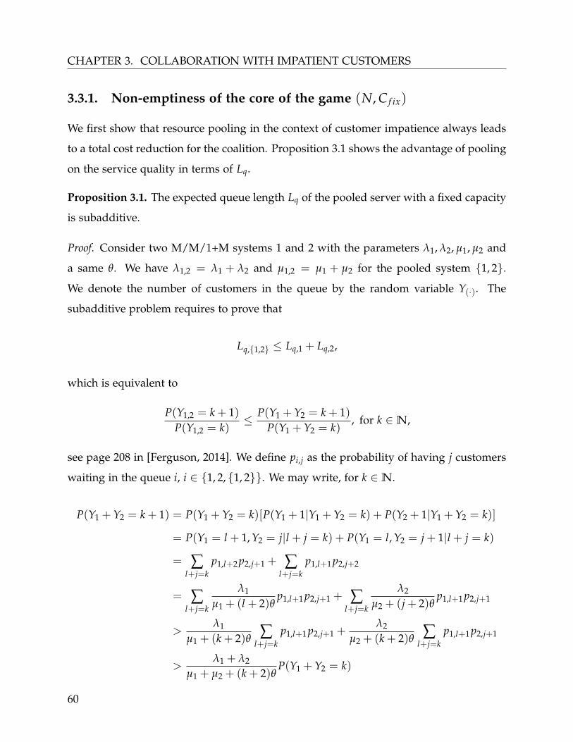
CHAPTER 3. COLLABORATION WITH IMPATIENT CUSTOMERS
3.3.1. Non-emptiness of the core of the game (N, C f ix)
We first show that resource pooling in the context of customer impatience always leads
to a total cost reduction for the coalition. Proposition 3.1 shows the advantage of pooling
on the service quality in terms of Lq.
Proposition 3.1. The expected queue length Lq of the pooled server with a fixed capacity
is subadditive.
Proof. Consider two M/M/1+M systems 1 and 2 with the parameters λ1, λ2, µ1, µ2 and
a same θ. We have λ1,2 = λ1 + λ2 and µ1,2 = µ1 + µ2 for the pooled system {1, 2}.
We denote the number of customers in the queue by the random variable Y(·). The
subadditive problem requires to prove that
Lq,{1,2} ≤ Lq,1 + Lq,2,
which is equivalent to
P(Y1,2 = k + 1)P(Y1,2 = k)
≤ P(Y1 + Y2 = k + 1)P(Y1 + Y2 = k)
, for k ∈ N,
see page 208 in [Ferguson, 2014]. We define pi,j as the probability of having j customers
waiting in the queue i, i ∈ {1, 2, {1, 2}}. We may write, for k ∈ N.
P(Y1 + Y2 = k + 1) = P(Y1 + Y2 = k)[P(Y1 + 1|Y1 + Y2 = k) + P(Y2 + 1|Y1 + Y2 = k)]
= P(Y1 = l + 1, Y2 = j|l + j = k) + P(Y1 = l, Y2 = j + 1|l + j = k)
= ∑l+j=k
p1,l+2p2,j+1 + ∑l+j=k
p1,l+1p2,j+2
= ∑l+j=k
λ1
µ1 + (l + 2)θp1,l+1p2,j+1 + ∑
l+j=k
λ2
µ2 + (j + 2)θp1,l+1p2,j+1
>λ1
µ1 + (k + 2)θ ∑l+j=k
p1,l+1p2,j+1 +λ2
µ2 + (k + 2)θ ∑l+j=k
p1,l+1p2,j+1
>λ1 + λ2
µ1 + µ2 + (k + 2)θP(Y1 + Y2 = k)
60
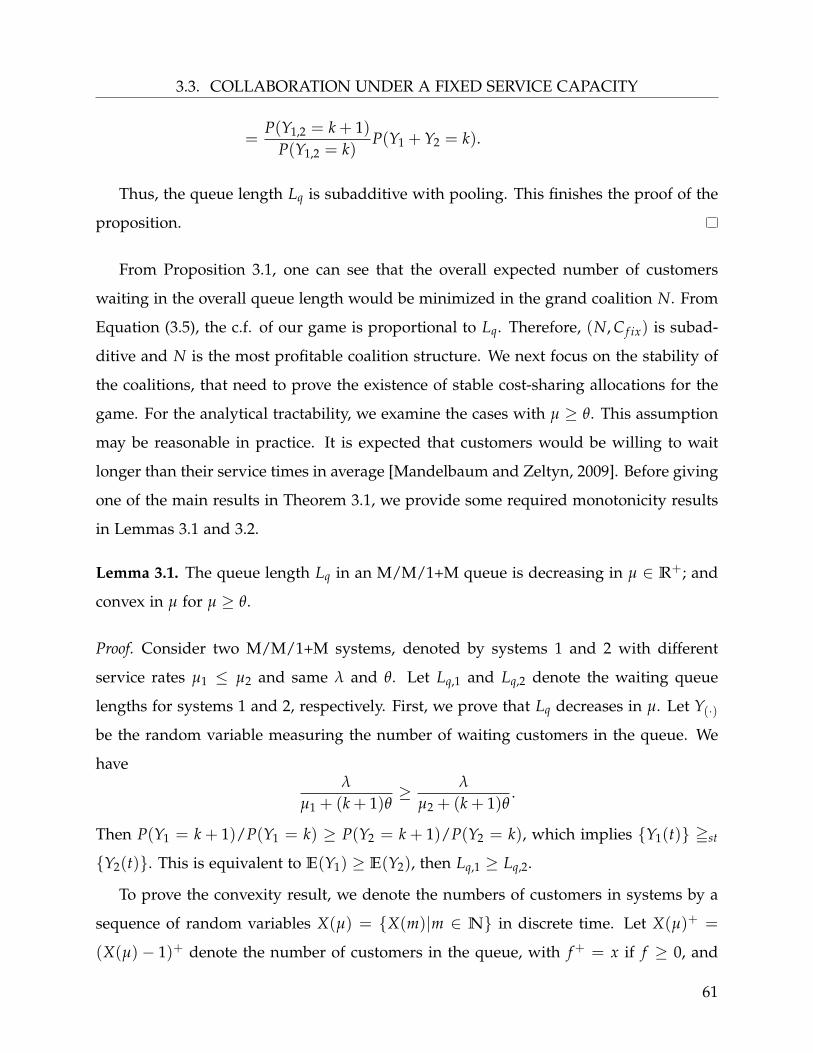
3.3. COLLABORATION UNDER A FIXED SERVICE CAPACITY
=P(Y1,2 = k + 1)
P(Y1,2 = k)P(Y1 + Y2 = k).
Thus, the queue length Lq is subadditive with pooling. This finishes the proof of the
proposition.
From Proposition 3.1, one can see that the overall expected number of customers
waiting in the overall queue length would be minimized in the grand coalition N. From
Equation (3.5), the c.f. of our game is proportional to Lq. Therefore, (N, C f ix) is subad-
ditive and N is the most profitable coalition structure. We next focus on the stability of
the coalitions, that need to prove the existence of stable cost-sharing allocations for the
game. For the analytical tractability, we examine the cases with µ ≥ θ. This assumption
may be reasonable in practice. It is expected that customers would be willing to wait
longer than their service times in average [Mandelbaum and Zeltyn, 2009]. Before giving
one of the main results in Theorem 3.1, we provide some required monotonicity results
in Lemmas 3.1 and 3.2.
Lemma 3.1. The queue length Lq in an M/M/1+M queue is decreasing in µ ∈ R+; and
convex in µ for µ ≥ θ.
Proof. Consider two M/M/1+M systems, denoted by systems 1 and 2 with different
service rates µ1 ≤ µ2 and same λ and θ. Let Lq,1 and Lq,2 denote the waiting queue
lengths for systems 1 and 2, respectively. First, we prove that Lq decreases in µ. Let Y(·)
be the random variable measuring the number of waiting customers in the queue. We
haveλ
µ1 + (k + 1)θ≥ λ
µ2 + (k + 1)θ.
Then P(Y1 = k + 1)/P(Y1 = k) ≥ P(Y2 = k + 1)/P(Y2 = k), which implies {Y1(t)} =st
{Y2(t)}. This is equivalent to E(Y1) ≥ E(Y2), then Lq,1 ≥ Lq,2.
To prove the convexity result, we denote the numbers of customers in systems by a
sequence of random variables X(µ) = {X(m)|m ∈ N} in discrete time. Let X(µ)+ =
(X(µ)− 1)+ denote the number of customers in the queue, with f+ = x if f ≥ 0, and
61

CHAPTER 3. COLLABORATION WITH IMPATIENT CUSTOMERS
x+ = 0 otherwise. As shown in Theorem 3 by [Armony et al., 2009], X is stochastically
decreasing and convex in sample path sense (denoted by SDCX(sp)) in µ with µ ≥ θ.
Because f = (x − 1)+ is increasing and convex, it follows that X+ is also SDCX(sp) by
Proposition 3.2(b) in [Shaked and Shanthikumar, 1988]. From Theorem 3.6 in [Shaked
and Shanthikumar, 1988], Lq = E(X+) is therefore decreasing and convex in µ with
µ ≥ θ. The lemma result follows.
Note that the convexity result in Lemma 3.1 is also verified for 0 < µ < θ through an
extensive numerical study, although we could not prove it rigorously.
Lemma 3.2. The abandonment probability Pa is increasing in the customer abandonment
rate θ ∈ [0,+∞).
Proof. Let us denote the mean number of customers in service by Ls. Let us also denote
by λa and λs the flows of abandonment and served rates, respectively. In the single
server system Ls = 1 − p0. Also, Ls is equal to the server’s utilisation ρs = λs/µ using
Little’s Law in [Little, 1961]. Thus,
Ls =λ − λa
µ=
λ − θLq
µ= 1 − p0
⇒ Pa =θLq
λ= 1 − µ
λ(1 − p0),
where p0 = (∑∞j=0 aj)
−1. It is obvious that aj as defined in Equation (3.2) is decreasing
in θ, for j ∈ N. Then, p0 is increasing in θ. The abandonment probability Pa is therefore
increasing in θ. The proof is completed.
Using Lemmas 3.1 and 3.2, we obtain the existence of stable cost allocations in Theo-
rem 3.1.
Theorem 3.1. The pooling game (N, C f ix) has a non-empty core for µ ≥ θ.
Proof. For any balanced collection B on N, we have
C f ix(N) = (cw + caθ)Lq(λN, µN)
62

3.3. COLLABORATION UNDER A FIXED SERVICE CAPACITY
= (cw + caθ)Lq(λN, ∑U∈B
βUµUλN
λU· λU
λN) (3.6)
≤ (cw + caθ) · ∑U∈B
βUλU
λNLq(λN, µU
λN
λU) (3.7)
= (cw + caθ) · ∑U∈B
βUλU
λNLq(λN, µU
λN
λU, θ)
= ∑U∈B
βU(cw + caθ) · λU
λNLq(λU, µU, θ
λU
λN)
≤ ∑U∈B
βU(cw + caθ) · Lq(λU, µU, θ) (3.8)
= ∑U∈B
βUC f ix(U).
From the definition of a balanced collection and the additivity of µ, it exists βU with
∑U∈B βUµU = µN to guarantee Equality (3.6). Inequality (3.7) holds by the convexity
property of Lq(µ) in Lemma 3.1 and βU with ∑U∈B βUλU = λN from the balanced
collection definition and the additivity of λ. Since Pa(θλUλN
) ≤ Pa(θ) (proved in Lemma
3.2) with θ λUλN
≤ θ and same λU, we have Lq(θλUλN
) · θ λUλN
≤ Lq(θ) · θ which leads to
the inequality in (3.8). Thus, the game (N, C f ix) is a balanced game. According to
"Bondareva-Shapley Theorem" in [Bondareva, 1963], the game (N, D f ix) has a non-empty
core, which completes the proof of the theorem.
3.3.2. Impact of abandonment on the stability of the Shapley value
From Theorem 3.1, we conclude that a core allocation always exists for the game (N, C f ix).
Thus, the explicit numerical solutions could be computed through a mathematical pro-
gramming method, such as the Nucleolus [Bondareva, 1963], the Equal Profit Method
[Frisk et al., 2010] or the EPM based on Contribution Weights [Peng et al., 2015]. To
the contrary to the case with no abandonments, we find that the presence of impatience
could impact the stability of the Shapley value for our game (N, C f ix). First of all, we
use an example of three players to illustrate this feature.
Example. As that shown in last chapter, the example of three players game among
63

CHAPTER 3. COLLABORATION WITH IMPATIENT CUSTOMERS
M/GI/1 service systems (relevant initial values in Table 3.1) is not concave and the
Shapley value could not provide a stable allocation.
PlayersParameters
λi µi Ci sh f ixi
1 9 10 8.1 3.13292 5 10 0.5 −0.90893 2 10 0.05 −1.6145
Table 3.1: 3 players pooling game
Let us now investigate the impact of abandonment on the stability of the Shapley
value, which is symbolized by sh f ix in (N, C f ix). For simplification, we choose cw = ca =
1 which does not affect the stability of the Shapley value. By the increasing of θ, we
numerically observe that sh f ix provides a stable allocation for θ ≥ 0.42. We denote this
value as the lower bound of the interval which has sh f ix in the core by θlow. In Table 3.2,
we calculate coalition and sh f ix distributed costs in this case for θ = 0, θlow and 1000.
CoalitionsC f ix(U) ∑i∈U sh f ix
i C f ix(U) ∑i∈U sh f ixi C f ix(U) ∑i∈U sh f ix
iθ = 0 θ = 0.42 θ = 1000
{1,2,3} 0.6095 0.6095 0.7827 0.7827 5.4647 5.4647{1,2} 1.6333 2.2240 1.7250 1.5205 5.7038 5.4766{2,3} 0.1885 −2.5234 0.2490 −0.7716 1.7902 1.5626{1,3} 0.6722 1.5184 0.8190 0.8165 3.8576 3.8902
Table 3.2: Coalition and distributed costs with θ = 0, 0.42 and 1000
The excess of a coalition U ⊆ N at x is defined as the quantity ex,U = C(U)− ∑i∈U xi,
i.e., the cost reduction of U by x, which is used to measure satisfaction of coalitions.
If ex,U ≤ 0, the coalition U would like to split off from N by using allocation x. From
the comparison between the first two columns in Table 3.2, we observe two unsatisfied
coalitions {1, 2} and {1, 3}, with esh f ix,{1,2} < 0 and esh f ix,{1,3} < 0 for θ = 0. It is to say
that 1 leaving N with 2 or 3 could form a more profitable smaller coalition. However, as
64

3.3. COLLABORATION UNDER A FIXED SERVICE CAPACITY
θ increases, esh f ix,{1,2} and esh f ix,{1,3} increase and grow gradually toward positive values
as shown in Figure 3.5. It means that the presence of θ enforces the stability of sh f ix in
this range.
Figure 3.5: esh f ix ,{1,2}, esh f ix ,{1,3} in θ for the 3 players game
By increasing θ, we observe that the coalition {1, 3} is no longer satisfied by sh f ix
for θ ≥ 382.4, i.e., esh f ix,{1,3} < 0. In a similar way, we denote this point by θup as the
upper bound of the stable interval of sh f ix. This interval is denoted by Θ = [θlow, θup).
When θ is much larger than λ and µ (θ = 1000 as given in Table 3.2), the players act as
M/M/1/1 queueing systems (no queue). We see that the same coalition {1, 3} obstruct
the grand coalition under sh f ix. Moreover, as θ → +∞, the system abandonment rate
converges to Pa = λ/(λ + µ) and the expected queue length Lq converges to 0. The
total cost function could be then calculated as, C f ix = caλ2/(λ + µ). This also leads
to an unsatisfied coalition {1, 3} for θ = 1000. More detailed illustrations with higher
numbers of players are given in Appendix B.
We observe that the Shapley value may lie at the core with the presence of customer
abandonment. Furthermore, we prove that it is in the core, when all providers have
identical offered loads (sh f ix is stable). Before giving the proof, we first need to analyze
the convexity of Lq in θ.
65

CHAPTER 3. COLLABORATION WITH IMPATIENT CUSTOMERS
Theorem 3.2. The expected queue length Lq of an M/M/1+M system is decreasing in
θ ∈ R+; and convex in θ for θ ≤ µ.
The proof of Theorem 3.2 is given in Appendix C. In this proof, we use sample-path
arguments similarly to [Armony et al., 2009], where the authors show a similar result
for the relationship between Lsys (the expected number of customers in the system) and
µ or the number of servers in Erlang-A model. Note that this convexity property is also
useful for various optimization studies in M/M/1+M queueing systems. Now, we are
ready to prove the stability of the Shapley value under the offered load constraint.
Proposition 3.2. The Shapley value is a core allocation for the game (N, C f ix), if λi/µi =
ρ for all i ∈ N and θ ≤ µ.
Proof. To prove the stability of the Shapley value, it suffices to prove the concavity of the
operational cost C f ix(ρµ, µ, θ) in the service rate µ. Consider any pair of coalitions U and
T with ∅ ⊆ U ⊂ T ⊂ N and a service provider l ∈ N \ T. We define θ0 as θ/µ. Since
C f ix is twice differentiable in µ, we have
∂2C f ix(ρµ, µ, θ)
∂µ2 =∂2C f ix(ρ, 1, θ/µ)
∂µ2
= (cw + caθ)∂2Lq(ρ, 1, θ0)
∂µ2
= (cw + caθ)[(− θ
µ2 ) ·∂2Lq∂θ2
0+
2θ
µ3 ·∂Lq
∂θ0] ≤ 0, (3.9)
where the inequality in (3.9) holds from ∂2Lq/∂θ2 ≥ 0 and ∂Lq/∂θ ≤ 0, which is based
on Theorem 3.2. Thus, C f ix is concave in µ if λi/µi = ρ. Furthermore, the Shapley value
stays in the core as shown in Theorem 7 in [Shapley, 1971]. This finishes the proof of the
proposition.
From Proposition 3.2, we then deduce that the Shapley value is a sufficient reasonable
cost allocation for a group of service providers with similar offered loads.
66

3.4. COLLABORATION UNDER THE OPTIMIZED SERVICE CAPACITY
3.4. Collaboration under the optimized service capacity
In certain cases, systems could be engineered. For example, the service capacity could be
increased according by training employees while may improve the service rate. Assum-
ing here that any individual or coalition chooses the service capacity which minimizes
the total system cost, this may lead to less costly coalitions. In this section, we consider
a TU-game under the setting with the optimized service capacity. We model the ser-
vice rate as a continuous variable for each individual or coalition. We denote by µ∗ the
optimized service capacity, which is defined by
µ∗(λ) = argmin{chµ + (cw + caθ)Lq(λ, µ, θ)|µ ≥ 0}. (3.10)
Figure 3.6: Total cost C in µ with different ch
Lemma 3.3. µ∗ exists and is unique in [θ,+∞).
Proof. C = chµ + (cw + caθ)Lq contains a linear function of µ and a term in Lq, which is
decreasing in µ and convex if µ ≥ θ (Lemma 3.1). Thus, C is positive and convex in µ if
µ ≥ θ. Therefore, µ∗ exists and is unique in [θ,+∞).
From Lemma 3.3, we obtain a unique optimized service capacity on its domain. Using
67

CHAPTER 3. COLLABORATION WITH IMPATIENT CUSTOMERS
(a) (b)
Figure 3.7: The optimized service capacity µ∗ in λ with different θ and ch
its definition in (3.10), it is obvious to see that µ∗ is decreasing in ch. An illustration is
given in Figure 3.6. For a coalition U = {1, ..., u} ∈ N, we also use the pooled arrival rate
λU = ∑i∈U λi and an identical abandonment rate θ as the defined game in Section 3.3.
Thus, we could define the optimized cost function using four parameters {θ, ch, ca, cw}
and a variable λi for i ∈ U as
Copt(λU) =ch · µ∗U(λU) + (cw + caθ)Lq(λU, µ∗
U(λU)),
with λU = ∑i∈U
λi, µ∗U = argmin{Ctotal|µ ≥ θ}, for any U ⊂ N. (3.11)
The pooling game under the optimized service capacity could be then defined as (N, Copt).
In order to propose a simple stable allocation rule, we next analyze the relationship be-
tween the total cost for one demand and λ.
Lemma 3.4. The total cost per unit demand with optimized service capacities Copt/λ, is
decreasing in the customer arrival rate λ.
Proof. Consider two M/M/1+M queues, denoted by 1 and 2, with λ1 ≤ λ2, µ∗1 , µ∗
2
(associated optimized service capacities) and a same θ. We have
Copt({1})λ1
= chµ∗
1λ1
+(cw + caθ)
λ1Lq(λ1, µ∗
1 , θ)
68

3.4. COLLABORATION UNDER THE OPTIMIZED SERVICE CAPACITY
= chµ∗
1λ1
+(cw + caθ)
λ1Lq(λ2, µ∗
1 ·λ2
λ1, θ
λ2
λ1)
≥ chµ∗
1λ1
+(cw + caθ)
λ1· λ1
λ2Lq(λ2, µ∗
1 ·λ2
λ1, θ) (3.12)
= chµ∗1 ·
λ2
λ1· 1
λ2+
(cw + caθ)
λ2Lq(λ2, µ∗
1 ·λ2
λ1, θ)
=1
λ2C(λ2, µ∗
1 ·λ2
λ1, θ) ≥
Copt({2})λ2
,
where Inequality (3.12) holds by the monotonicity of Pa in θ in Lemma 3.2. Thus, Copt/λ
decreases in λ. This finishes the proof of the lemma.
From Lemma 3.4, we could conclude that the following allocation rule provides a
PMAS for the game (N, Copt):
φpi =
λi
λNCopt(N), ∀i ∈ N. (3.13)
Proposition 3.3. The propositional allocation φp defined in Equation (3.13) is a core
allocation for the game (N, Copt), and the associated allocation scheme φas,p gives a
PMAS for this game.
As proved in Section 2.5.2, the game with θ = 0 provides a concave TU-game. We
next consider the other limit for θ much higher than λ and µ, i.e., where a provider
approaches an M/M/1/1 queue. We rewrite the cost function as
Copt = chµ + caλ2
λ + µ. (3.14)
With this cost function, we could obtain the optimized service rate as follows.
µ∗ =
(√
ca/ch − 1)λ, if ca > ch
0, otherwise.(3.15)
When ca ≤ ch, we get µ∗ = 0. It means that the optimal choice of the server is not
working. In the remaining case, the total cost Copt is linear with λ and the game (N, Copt)
turns to a linear game.
69

CHAPTER 3. COLLABORATION WITH IMPATIENT CUSTOMERS
3.5. Conclusion
We considered the pooling problem for service systems while accounting for the im-
portant feature of customer abandonment. We investigated the cooperative strategy
among independent service providers with a complete service capacity pooling. When
the service providers directly combine their queues and service capacities, we proved
the non-emptiness of the core under the situation with a fixed service capacity. With
customer abandonment, the stability of the Shapley value could be affected. We studied
the convexity of the expected queue length in the abandonment rate. This result is also
helpful when addressing other design issues. Furthermore, we found that if all service
providers have an identical offered load, the Shapley value is absolutely stable for our
game. Under the optimized service capacity, we proved that a simple proportional allo-
cation rule provides a stable allocation for the relative game. This chapter and Chapter
2 are both assumed in the ’super-server’ pooling environment. We will consider the
multi-server pooling case in the next chapter.
70

Chapter 4
Collaboration for Multi-server Service Sys-
tems
In Chapters 2 and 3, we analyzed resource pooling strategies under ’super-
server’ assumptions. In this chapter, we study the effect of resource pooling on
system performance and profit for multi-server service systems incorporating
customer abandonment, with the goal of evaluating whether the results under
the ’super-server’ assumption are still suitable in the multi-server case.
We consider two single-class queueing systems with different setting of pooling,
i.e., using the ’super-server’ assumptions and another using identical parallel
servers. The pooling strategy efficiency is estimated via the expected number of
customers in each system and the mean probability of customer abandonment.
Although it is intuitive to expect efficiency improvements in the pooled multi-
server system, it is no longer obvious to conclude that all members will benefit
from pooling as we proved in previous chapters. We compare between the two
71

CHAPTER 4. COLLABORATION FOR MULTI-SERVER SERVICE SYSTEMS
pooling settings from a coalition perspective. We numerically evaluate the ef-
fects of service duration variability and customer abandonment on the two cor-
responding games using the Shapley value and the nucleolus allocations. Fur-
thermore, we show that the service pooling in multi-class systems, is not always
profitable because of the additional variability among customer classes.
72

4.1. INTRODUCTION
4.1. Introduction
In this chapter, we address the service pooling problem for multi-server pooling system-
s. We allow that customers to be impatient in each individual or pooled service system.
They might decide to leave (abandon) before their services begin when their waiting
times are expired. We compare two corresponding TU-games of two typical pooling
settings and analyze dependent service pooling problems using cooperative game theo-
ry. In the rich literature on capacity pooling research, there are two typical settings for
the pooled systems: the ’super-server’ setting, i.e., all services resources are pooled in
one single server, and the multi-server setting, i.e., all servers work in parallel in a com-
mon service factory. Various examples of both setting are discussed in [Kleinrock, 1976].
The two pooling settings have been extensively used to evaluate the overall gains from
pooling by comparing the system performance of the pooled system and the individual
systems [Mandelbaum and Reiman, 1998, Iyer and Jain, 2004, Tekin et al., 2014, Kim and
Kim, 2015, Andradóttir et al., 2017]. The main reason for the ’super-server’ assump-
tion is that dealing with multi-server queues with general service times and customer
abandonment is very hard, even for a system with homogeneous servers. One known
approximation idea in homogeneous service cases that works quite well for the design of
services is the asymptotic equivalence in heavy traffic resource pooling cases [Harrison
and López, 1999].
The purpose of this chapter is to get a deeper understanding about whether pooling
strategies can be implemented to attain a higher service performance and a better col-
laboration income in real-life systems. In Chapters 2 and 3, we analyzed the cost-sharing
problem in service pooling collaboration with general service times and impatient cus-
tomers in the ’super-server’ pooling setting. This assumption is also accepted in many
other related service pooling studies [Anily and Haviv, 2010, Anily and Haviv, 2014, Yu
et al., 2015]. Motivated by applications to real-life systems, it is reasonable to extend
our previous research in multi-server systems [Özen et al., 2011, Karsten et al., 2015b],
especially in queueing systems accounting for customer abandonment from queue ow-
73

CHAPTER 4. COLLABORATION FOR MULTI-SERVER SERVICE SYSTEMS
ing to customer impatience. Such systems are widely used in service system design,
e.g., the many-server heavy-traffic queueing model in call center applications [Dai and
He, 2010, Jouini et al., 2013], the emergency hospital modeling problem [Gunal, 2012].
Therefore, we consider the stationary M/GI/S+M queuing model to describe the multi-
server service system. In order to evaluate the ’super-server’ assumptions, we use the
M/GI/1+M modeling for the individual and the ’super-server’ pooling system. Given
the complexity of the analysis of the M/GI/S+M queue, we conduct a simulation study
to compare between the two pooling situations.
The remainder of this chapter is structured as follows. We start in Section 4.2 by
defining all notations of our models and deriving some comparisons for the pooling
gains. Next, in Section 4.3, we provide a brief analysis of the relative service pooling
game in case of the markovian service process. In Section 4.4, we numerically analyze
the distributed costs with the impact of the variability of service times and the customer
arrival rates for the two games. In Section 4.5, we consider the impact of the customer
variability on service pooling gains. Finally, we give concluding comments.
4.2. Models and preliminary study
4.2.1. Service pooling modeling
We consider a set of N = {1, ..., n}, n ∈ N+ independent single-server service providers,
a provider is denoted by i ∈ N. We address here the individual setting (without pooling),
the ’super-server’ setting (a single-server with a high service rate) and the multi-server
setting (a pooled queue with parallel servers).
Individual service system i
In the individual setting, each provider is associated with its own Poisson customer ar-
rival stream of rate λi, which does not affect other providers. All customers in the set N
are assumed to be classified in a same class, i.e., same priority for service. The waiting
74

4.2. MODELS AND PRELIMINARY STUDY
space is assumed to be large enough such that no customer would be refused by the
server. We assume that all the servers are identical, and service times are assigned to
servers, which are i.i.d. and follow a general distribution with mean 1/µ and coefficient
of variation cv. The first come, first served (FCFS) discipline is used. Let customers be
impatient. Patience times are assumed to be i.i.d. and exponentially distributed with
mean 1/θ. If a customer has waited in the queue longer than his patience limit, he
quits the waiting queue without a service. We assume that θ ≤ µ to limit the aban-
donment rate. Following these arguments, each service provider can be modeled as an
M/GI/1+M queueing system (Figure 4.1), denoted by Sysi, i ∈ N.
Figure 4.1: An individual service provider i, an M/GI/1+M queue
’Super-server’ pooling coalition U
For a subset U = {1, ..., u} ⊆ N of u service providers, we assume that they could operate
their service capacities together to form a ’super-server’. The pooling system has a
Poisson customer arrival stream of rate λU = ∑i∈U λi. The waiting space is large enough,
and FCFS is employed. In the pooling set, we assume that the overall service capacity is
equivalent to the sum of the capacities of the u individual providers in U. Consequently,
service times are assigned to the pooled server, i.i.d. and generally distributed with mean
1/µU, µU = uµ and coefficient of variation cv. Patience times are assigned to customers,
i.i.d. and exponentially distributed with mean 1/θ. The u providers are combined into a
new M/GI/1+M queueing system (Figure 4.2), denoted by SyssU, U ⊆ N. We have used
a similar definition to define resource pooling in Chapters 2 and 3 for any given µi for
server i.
75

CHAPTER 4. COLLABORATION FOR MULTI-SERVER SERVICE SYSTEMS
Figure 4.2: ’super-server’ pooling concept in U = {1, ...u}, an M/GI/1+M queue
Multi-server pooling coalition U
We consider a subset U = {1, ..., u} ⊆ N of u service providers, they could operate
their servers together to provide same services for all customers. We assume that all
the u servers are parallel and identical to all customers in U. Using similar assumptions
in ’super-server’ setting, the u providers are combined into an M/GI/S+M queueing
system. The customer arrival stream follows a Poisson process with rate λU = ∑i∈U λi,
and patience times are i.i.d. and exponentially distributed with mean 1/θ. Service times
are assigned to servers, i.i.d. and general distributed with mean 1/µ and coefficient of
variation cv. The multi-server pooling coalition U is shown in Figure 4.3, denoted by
SysmU, U ⊆ N.
Figure 4.3: Multi-server pooling concept in U = {1, ...u}, an M/GI/S+M queue
76
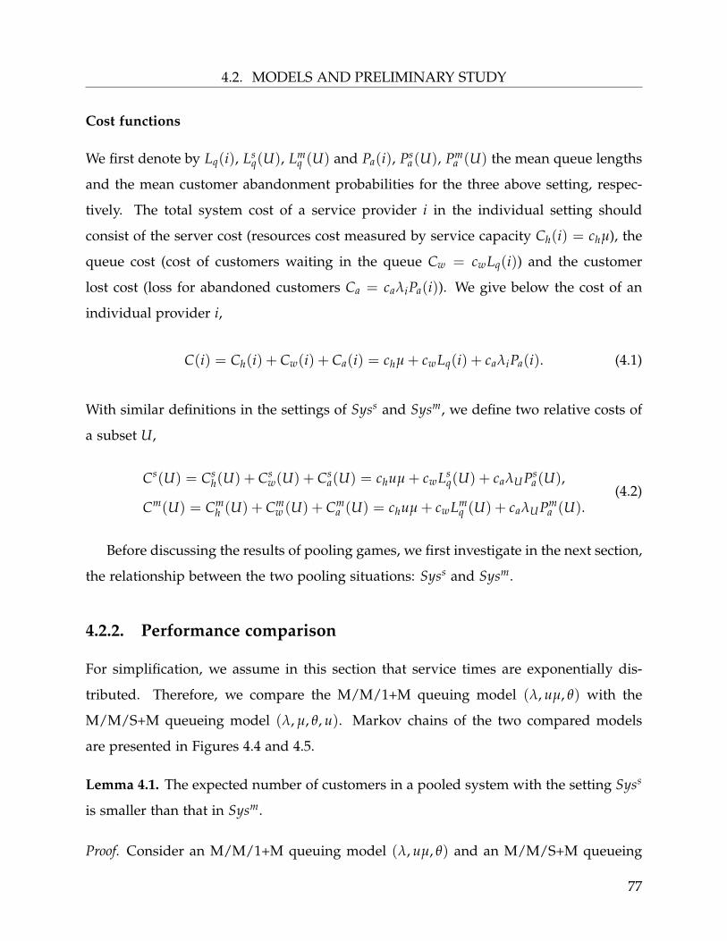
4.2. MODELS AND PRELIMINARY STUDY
Cost functions
We first denote by Lq(i), Lsq(U), Lm
q (U) and Pa(i), Psa(U), Pm
a (U) the mean queue lengths
and the mean customer abandonment probabilities for the three above setting, respec-
tively. The total system cost of a service provider i in the individual setting should
consist of the server cost (resources cost measured by service capacity Ch(i) = chµ), the
queue cost (cost of customers waiting in the queue Cw = cwLq(i)) and the customer
lost cost (loss for abandoned customers Ca = caλiPa(i)). We give below the cost of an
individual provider i,
C(i) = Ch(i) + Cw(i) + Ca(i) = chµ + cwLq(i) + caλiPa(i). (4.1)
With similar definitions in the settings of Syss and Sysm, we define two relative costs of
a subset U,
Cs(U) = Csh(U) + Cs
w(U) + Csa(U) = chuµ + cwLs
q(U) + caλUPsa(U),
Cm(U) = Cmh (U) + Cm
w (U) + Cma (U) = chuµ + cwLm
q (U) + caλUPma (U).
(4.2)
Before discussing the results of pooling games, we first investigate in the next section,
the relationship between the two pooling situations: Syss and Sysm.
4.2.2. Performance comparison
For simplification, we assume in this section that service times are exponentially dis-
tributed. Therefore, we compare the M/M/1+M queuing model (λ, uµ, θ) with the
M/M/S+M queueing model (λ, µ, θ, u). Markov chains of the two compared models
are presented in Figures 4.4 and 4.5.
Lemma 4.1. The expected number of customers in a pooled system with the setting Syss
is smaller than that in Sysm.
Proof. Consider an M/M/1+M queuing model (λ, uµ, θ) and an M/M/S+M queueing
77

CHAPTER 4. COLLABORATION FOR MULTI-SERVER SERVICE SYSTEMS
Figure 4.4: The Markov process, an M/M/1+M queueing model
Figure 4.5: The Markov process, an M/M/S+M queueing model
model (λ, µ, θ, u). We denote the number of customers in the two systems by the random
variable Y(·). The problem is to prove that
Lss(U) = E(Ys) ≤ Lm
s (U) = E(Ym),
which is equivalent to
P(Ys = k + 1)Ys = k
≤ P(Ym = k + 1)Ym = k
, for k ∈ N,
see page 208 in [Ferguson, 2014]. From Markov chains in Figures 4.4 and 4.5, we have
P(Ys = k + 1)Ys = k
=λ
uµ + kθ≤ λ
kµ=
P(Ym = k + 1)Ym = k
, for 0 ≤ k < µ;
P(Ys = k + 1)Ys = k
=λ
uµ + kθ≤ λ
uµ + (k + 1 − u)θ=
P(Ym = k + 1)Ym = k
, for k ≥ µ.
Thus, the expected number of customers Ls in the M/M/1+M system is smaller, which
completes the proof of the proposition.
From Lemma 4.1, one can see that the overall expected number of customers in the
setting Syss is smaller than that in Sysm, without any limit for the system parameters
78

4.3. SERVICE POOLING GAMES
{λ, µ, θ, u)}. The comparison of the queue length could be illustrated with a similar
reasoning. We denote the number of customers in the two systems by the random
variable Y−(·). Thus, we have identical P(Y−
(·) = k + 1)/P(Y−(·) = k) for all k ∈ N+. The
only difference is the value at k = 0. With a simple calculation, we can obtain Lemma
4.2
Lemma 4.2. The queue length in the setting Syss is larger than that in Sysm.
From the customer’s point of view, we see that customers spend less overall time in
Syss but wait more time in queue. This phenomenon is well known in queueing systems
without customer abandonment [Monahan, 2000]. When customers are impatient, Syss
loses more customers than Sysm dose. This reduces the difference between Lsq and Lm
q .
4.3. Service pooling games
In order to analyze the pooling strategies, we construct two corresponding service pool-
ing games. We assume that every service provider i (player i) in the set N (the grand
coalition) is economically independent. Suppose that a subset U, ∅ ⊆ U ⊆ N, form-
s a coalition. In the coalition, providers operate their service resources together with
pooling strategies. In above section, we assume that the service capacity in the pooling
system is the sum of the individuals’. Thus, the server cost C(·)h is additive, which is
meaningless in cooperative game study. The service pooling gain is only captured by
C(·)w and C(·)
a . Consider that the abandonment process is Markovian. Therefore, for any
coalition U ⊆ N, we denote the cost functions by
Cs(∅) = 0, Cs(U) = Csw(U) + Cs
a(U) = (cw + caθ)Lsq(U) ∈ R+;
Cm(∅) = 0, Cm(U) = Cmw (U) + Cm
a (U) = (cw + caθ)Lmq (U) ∈ R+,
(4.3)
under corresponding service pooling strategy, respectively. The pairs (N, Cs) and (N, Cm)
define two cooperative games with transferable utility (TU-game). In particular, Cs(·)
and Cm(·) are theirs characteristic functions (c.f.).
79
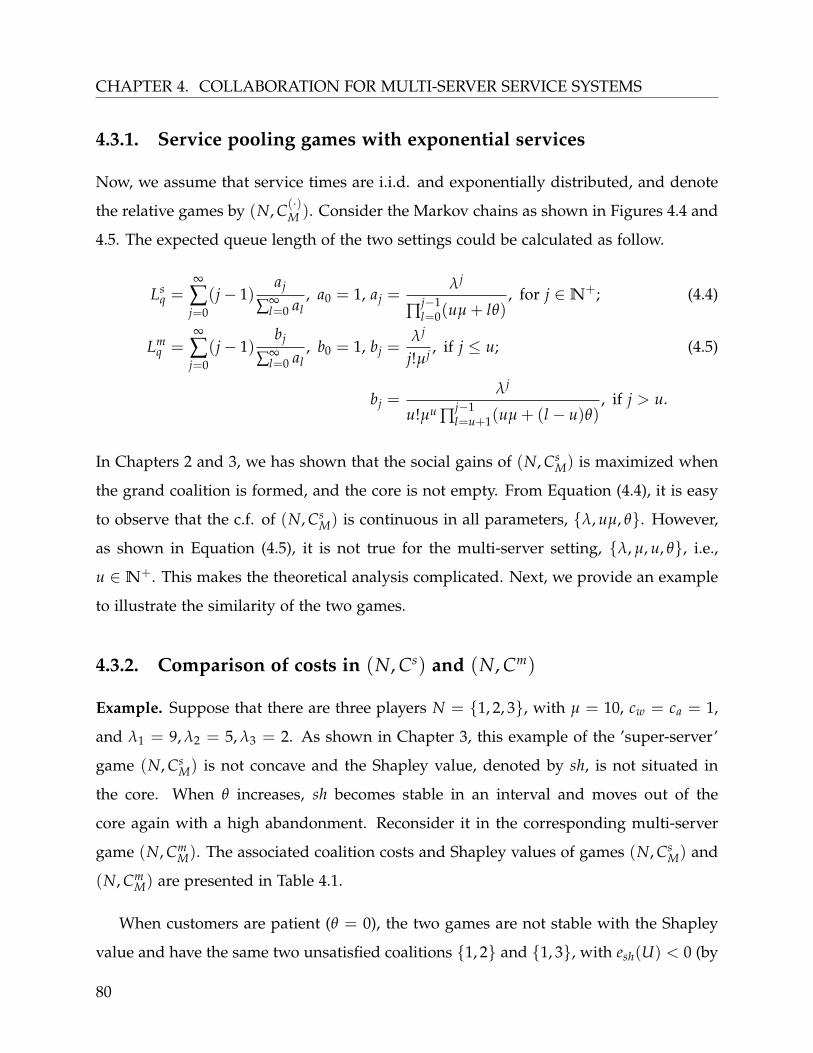
CHAPTER 4. COLLABORATION FOR MULTI-SERVER SERVICE SYSTEMS
4.3.1. Service pooling games with exponential services
Now, we assume that service times are i.i.d. and exponentially distributed, and denote
the relative games by (N, C(·)M ). Consider the Markov chains as shown in Figures 4.4 and
4.5. The expected queue length of the two settings could be calculated as follow.
Lsq =
∞
∑j=0
(j − 1)aj
∑∞l=0 al
, a0 = 1, aj =λj
∏j−1l=0(uµ + lθ)
, for j ∈ N+; (4.4)
Lmq =
∞
∑j=0
(j − 1)bj
∑∞l=0 al
, b0 = 1, bj =λj
j!µj , if j ≤ u; (4.5)
bj =λj
u!µu ∏j−1l=u+1(uµ + (l − u)θ)
, if j > u.
In Chapters 2 and 3, we has shown that the social gains of (N, CsM) is maximized when
the grand coalition is formed, and the core is not empty. From Equation (4.4), it is easy
to observe that the c.f. of (N, CsM) is continuous in all parameters, {λ, uµ, θ}. However,
as shown in Equation (4.5), it is not true for the multi-server setting, {λ, µ, u, θ}, i.e.,
u ∈ N+. This makes the theoretical analysis complicated. Next, we provide an example
to illustrate the similarity of the two games.
4.3.2. Comparison of costs in (N, Cs) and (N, Cm)
Example. Suppose that there are three players N = {1, 2, 3}, with µ = 10, cw = ca = 1,
and λ1 = 9, λ2 = 5, λ3 = 2. As shown in Chapter 3, this example of the ’super-server’
game (N, CsM) is not concave and the Shapley value, denoted by sh, is not situated in
the core. When θ increases, sh becomes stable in an interval and moves out of the
core again with a high abandonment. Reconsider it in the corresponding multi-server
game (N, CmM). The associated coalition costs and Shapley values of games (N, Cs
M) and
(N, CmM) are presented in Table 4.1.
When customers are patient (θ = 0), the two games are not stable with the Shapley
value and have the same two unsatisfied coalitions {1, 2} and {1, 3}, with esh(U) < 0 (by
80

4.4. NUMERICAL EXAMPLES
Coalitionsθ = 0 θ = 0.5
CsM(U) ∑i∈U shs
i CmM(U) ∑i∈U shm
i CsM(U) ∑i∈U shs
i CmM(U) ∑i∈U shm
i
{1, 2, 3} 0.6095 0.6095 0.3130 0.3130 0.8130 0.8130 0.4135 0.4135{1, 2} 1.6333 2.2240 1.3451 1.9779 1.7520 1.5285 1.4185 1.2139{2, 3} 0.1885 -2.5234 0.0977 -2.6700 0.2597 -0.7218 0.1342 -0.9326{1, 3} 0.6722 1.5184 0.4771 1.3189 0.8447 0.5958 0.5940 0.5457
Table 4.1: Coalition and distributed costs with θ = {0, 0.5} for (N, CsM) and (N, Cm
M)
comparing data of Table 4.1). By increasing θ, we numerically observe that the Shapley
value is situated in the core for the two games. This phenomenon appears also with
another services and the cases with higher number of players. In the next section, we
give a systemic numerical comparison for three players games.
4.4. Numerical examples
We perform a simulation study in order to evaluate and compare the service pooling
cost-sharing problem of the two strategies. The main reason of the simulation lies in the
analytical complexity of the M/GI/S+M analysis and the intractable theoretical treat-
ment of the related pooling games. Simulation is done with Matlab. We simulate the two
pooling settings in three players set with deterministic, Erlang-2 (cv = 1/√
2 = 0.707)
and hyperexponential (i.e., µh,1 = {0.5µ + 1.5µ}, p1 = {0.25, 0.75}, cv = 1.291 and
µh,2 = {0.2899µ + 2.5798µ}, p2 = {0.2, 0.8}, cv = 2) services and calculate the corre-
sponding exponential situation. From the identical servers assumption, i.e., same µ, the
individual utilization ρi = λi/µ of each server depends on own customer incoming rate.
Therefore, we initially consider the case µ = 10 and λ = {1, ...9}. We choose 20 cases
of triples λ = (λ1, λ2, λ3) to evaluate the cost allocations using the Shapley value sh and
the nucleolus φn. The overall cost of each individual player or coalition is calculated by
Equation (4.3) with cw = ca = 1. We choose this setting because the contrast between
different customer incoming rates is the biggest reason for cost distribution and three
81

CHAPTER 4. COLLABORATION FOR MULTI-SERVER SERVICE SYSTEMS
players game is a typical case for cost-sharing analysis. For evaluating the impact of cus-
tomer abandonment, we choose four values θ = {0, 0.5, 1, 3}. This gives us 80 different
configurations for each game for each service distribution.
In all numerical tests, we find that the nucleolus is always situated in the core. It
presents the non-emptiness of the core for all numerical examples. It means that the
grand coalition is the most profitable coalition structure, and the three service provider-
s would agree on pooling their service resources. Given the relationship shown for
Markovian systems, the overall costs of Syss are always larger than Sysm in all cases.
Considering this difference between the two pooling settings, we calculate the individ-
ual saving in overall pooling saving by percentage in the grand coalition N = {1, 2, 3},
sp(·)x,i = [C(·)({i})− x(·)i ]/[∑i∈N C(·)({i})− C(·)(N)]%, i.e., x = (x1, ..., xn) present a cost
allocation in N. Therefore, we give some cases in Tables 4.2. The first three cases are
the cases with heterogeneous λ, and homogeneous λ are selected in last three cases.
’Y’(Yes), ’N’(No),’N-Y’(No-Yes) indicate the stability of φ, and ’N-Y’ means that the sta-
bility changes with service times variability in these cases.
4.4.1. Impact of customer arrival rates λi
The λi is the only individual parameter for each service provider i. Thus, its heterogene-
ity leads to heterogeneity in allocated costs. From Table 4.2, it is shown that the saving
percentages using both the Shapley value or the Nucleolus allocations of Sysm and Syss
pooling systems are very closed in all the cases. The stabilities of the sh for the two
pooling concepts are also very similar in the majority of cases, which varies with the ser-
vice variability cv and the customer abandonment rate θ. The special situations appear
for the cases of (1, 1, 2), in which all the three players have low initial utilizations. It is
also shown that the sh is not stable for these cases with heterogeneous λi when θ = 0,
i.e., (1, 2, 9) with two small and one large λi, and (1, 5, 9) with three heterogeneous λi.
However, the sh is stable in the case (1, 8, 9), i.e., one small and two large λi.
82

4.4. NUMERICAL EXAMPLES
λi ∈ N cv θ = 0 θ = 0.5sps
sh% spmsh% sps
n% spmn % sps
sh% spmsh% sps
n% spmn %
(1, 2, 9)
017.93% 17.88% 2.71% 2.54% 19.85% 19.37% 6.80% 6.05%17.08% 17.11% 1.86% 1.77% 17.67% 18.14% 4.62% 4.82%64.99% 65.00% 95.44% 95.68% 62.48% 62.49% 88.58% 89.14%
0.70717.84% 17.81% 2.51% 2.39% 20.27% 19.79% 7.71% 6.89%17.04% 17.11% 1.70% 1.69% 17.88% 18.40% 5.33% 5.50%65.12% 65.09% 95.79% 95.91% 61.86% 61.82% 86.96% 87.60%
117.90% 17.81% 2.64% 2.44% 20.71% 20.32% 8.74% 7.90%17.06% 17.16% 1.79% 1.79% 18.13% 18.47% 6.16% 6.04%65.04% 65.03% 95.57% 95.76% 61.16% 61.21% 85.10% 86.06%
1.29117.94% 17.93% 2.72% 2.64% 21.44% 20.78% 10.23% 8.88%17.07% 17.14% 1.85% 1.85% 18.25% 18.70% 7.03% 6.79%65.00% 64.93% 95.44% 95.52% 60.30% 60.52% 82.74% 84.33%
218.19% 17.71% 3.12% 2.33% 22.57% 21.08% 12.62% 9.69%16.98% 17.28% 1.91% 1.89% 18.57% 19.32% 8.62% 7.93%64.83% 65.02% 94.97% 95.78% 58.86% 59.60% 78.75% 82.38%
Stability N N Y Y N N Y Y
(1, 5, 9)
021.25% 21.04% 8.09% 7.92% 26.19% 25.41% 17.07% 16.23%17.16% 17.61% 3.14% 3.53% 18.45% 19.64% 7.49% 8.45%61.59% 61.35% 88.77% 88.55% 55.36% 54.95% 75.43% 75.31%
0.70720.92% 20.90% 7.53% 7.67% 27.53% 26.45% 19.48% 18.24%17.18% 17.57% 2.97% 3.40% 18.66% 20.12% 8.46% 9.57%61.90% 61.53% 89.50% 88.92% 53.81% 53.43% 72.05% 72.19%
121.13% 20.83% 7.87% 7.60% 28.05% 26.87% 20.55% 19.13%17.16% 17.71% 3.08% 3.56% 19.05% 20.53% 9.20% 10.30%61.72% 61.45% 89.05% 88.84% 52.91% 52.59% 70.25% 70.57%
1.29121.56% 21.22% 8.61% 8.29% 29.04% 28.01% 22.30% 21.14%17.11% 17.71% 3.24% 3.75% 19.26% 20.74% 10.11% 11.26%61.33% 61.06% 88.15% 87.96% 51.69% 51.24% 67.60% 67.60%
221.15% 20.73% 7.86% 7.44% 29.21% 28.01% 23.21% 21.85%17.10% 17.79% 3.07% 3.61% 20.69% 22.49% 11.81% 13.33%61.75% 61.48% 89.07% 88.95% 50.10% 49.49% 64.98% 64.82%
Stability N N Y Y N-Y N-Y Y Y
(1, 8, 9)
029.50% 28.94% 25.67% 24.54% 34.58% 33.64% 35.82% 33.94%23.85% 24.40% 14.37% 15.47% 27.07% 27.85% 20.81% 22.37%46.65% 46.66% 59.96% 59.98% 38.35% 38.51% 43.37% 43.69%
0.70729.91% 28.92% 26.42% 24.51% 35.38% 33.68% 37.43% 34.02%23.02% 23.85% 12.85% 14.36% 27.11% 28.38% 20.89% 23.42%47.07% 47.23% 60.74% 61.12% 37.51% 37.95% 41.68% 42.56%
129.31% 28.71% 25.29% 24.10% 35.55% 34.07% 37.76% 34.82%23.89% 24.52% 14.46% 15.71% 27.45% 28.51% 21.56% 23.69%46.79% 46.77% 60.25% 60.20% 37.00% 37.41% 40.67% 41.49%
1.29130.20% 28.89% 27.07% 24.46% 35.43% 35.15% 37.53% 36.96%23.38% 24.48% 13.42% 15.63% 28.55% 28.86% 23.77% 24.38%46.42% 46.62% 59.50% 59.91% 36.02% 36.00% 38.70% 38.66%
229.74% 27.49% 26.14% 21.65% 36.26% 33.57% 39.20% 33.81%24.76% 26.24% 16.19% 19.15% 28.42% 29.96% 23.50% 26.59%45.50% 46.27% 57.67% 59.20% 35.32% 36.47% 37.30% 39.60%
Stability Y Y Y Y Y Y Y Y
Table 4.2: (a). Heterogeneous λi three players games
83

CHAPTER 4. COLLABORATION FOR MULTI-SERVER SERVICE SYSTEMS
λi ∈ N cv θ = 1 θ = 3sps
sh% spmsh% sps
n% spmn % sps
sh% spmsh% sps
n% spmn %
(1, 2, 9)
020.57% 20.36% 8.61% 8.01% 22.35% 21.64% 12.41% 10.95%18.16% 18.42% 6.20% 6.07% 18.95% 19.51% 9.01% 8.83%61.26% 61.22% 85.18% 85.92% 58.70% 58.84% 78.58% 80.22%
0.70721.51% 20.79% 10.44% 8.99% 22.89% 22.24% 13.70% 12.21%18.44% 18.87% 7.36% 7.06% 19.49% 20.05% 10.30% 10.01%60.05% 60.34% 82.20% 83.95% 57.62% 57.71% 76.00% 77.77%
121.72% 21.21% 10.95% 9.85% 23.42% 22.68% 14.72% 13.15%18.62% 19.06% 7.85% 7.71% 19.52% 20.26% 10.82% 10.73%59.67% 59.73% 81.20% 82.44% 57.06% 57.06% 74.46% 76.12%
1.29122.22% 21.35% 12.14% 10.30% 23.85% 23.10% 15.36% 14.04%18.77% 19.38% 8.69% 8.33% 19.54% 20.53% 11.05% 11.48%59.01% 59.27% 79.17% 81.37% 56.60% 56.36% 73.59% 74.48%
222.59% 22.06% 13.34% 11.85% 24.02% 23.18% 16.44% 14.64%19.71% 20.09% 10.47% 9.88% 20.45% 21.46% 12.87% 12.92%57.71% 57.85% 76.19% 78.28% 55.53% 55.36% 70.69% 72.44%
Stability N-Y N Y Y N-Y N-Y Y Y
(1, 5, 9)
027.90% 27.19% 20.32% 19.54% 30.32% 28.84% 25.08% 23.17%19.16% 20.36% 9.30% 10.39% 20.60% 22.25% 12.29% 13.53%52.93% 52.46% 70.39% 70.07% 49.08% 48.91% 62.63% 63.30%
0.70728.99% 27.87% 22.48% 21.16% 31.32% 29.08% 27.04% 24.01%19.92% 21.27% 10.83% 11.71% 21.24% 23.24% 13.69% 14.81%51.09% 50.85% 66.69% 67.12% 47.43% 47.67% 59.27% 61.18%
129.58% 28.08% 23.54% 21.67% 31.64% 29.49% 27.66% 24.85%19.91% 21.69% 11.09% 12.37% 21.32% 23.67% 13.90% 15.60%50.50% 50.23% 65.38% 65.96% 47.03% 46.84% 58.44% 59.56%
1.29130.29% 28.01% 24.88% 21.83% 32.66% 29.52% 29.49% 25.15%20.27% 22.30% 11.93% 12.96% 21.15% 24.27% 13.97% 16.34%49.44% 49.70% 63.19% 65.21% 46.19% 46.20% 56.54% 58.51%
231.28% 29.18% 26.99% 24.20% 32.17% 29.69% 28.99% 25.77%20.83% 23.45% 12.79% 15.20% 22.29% 25.30% 15.29% 17.82%47.89% 47.38% 60.22% 60.60% 45.54% 45.01% 55.72% 56.41%
Stability Y Y Y Y Y Y Y Y
(1, 8, 9)
035.89% 33.98% 38.44% 34.63% 35.90% 34.57% 38.48% 35.81%27.18% 28.39% 21.03% 23.44% 28.47% 29.48% 23.61% 25.64%36.93% 37.63% 40.53% 41.93% 35.62% 35.94% 37.92% 38.55%
0.70736.01% 34.53% 38.69% 35.72% 36.69% 34.68% 40.04% 36.02%28.02% 28.90% 22.70% 24.46% 28.51% 29.80% 23.68% 26.27%35.97% 36.58% 38.61% 39.82% 34.80% 35.52% 36.27% 37.71%
136.16% 34.39% 38.99% 35.44% 36.88% 34.43% 40.42% 35.52%27.94% 29.16% 22.55% 25.00% 28.51% 30.11% 23.69% 26.88%35.90% 36.45% 38.47% 39.56% 34.61% 35.46% 35.89% 37.60%
1.29135.99% 34.65% 38.65% 35.96% 37.27% 34.70% 41.21% 36.06%27.84% 29.06% 22.34% 24.79% 28.61% 30.31% 23.89% 27.28%36.17% 36.29% 39.01% 39.25% 34.12% 34.99% 34.90% 36.65%
237.82% 34.06% 42.31% 34.79% 38.55% 33.64% 43.77% 33.95%28.30% 30.45% 23.26% 27.57% 28.23% 31.06% 23.13% 28.79%33.88% 35.49% 34.43% 37.64% 33.22% 35.29% 33.10% 37.26%
Stability Y Y Y Y Y Y Y Y
Table 4.2: (b). Heterogeneous λi three players games
84

4.4. NUMERICAL EXAMPLES
λi ∈ N cv θ = 0 θ = 0.5sps
sh% spmsh% sps
n% spmn % sps
sh% spmsh% sps
n% spmn %
(1, 1, 2)
025.94% 25.73% 18.60% 18.11% 25.45% 25.61% 17.56% 17.97%25.94% 25.73% 18.60% 18.11% 25.45% 25.61% 17.56% 17.97%48.20% 48.49% 62.90% 63.75% 49.12% 48.72% 65.19% 64.06%
0.70725.55% 25.43% 17.78% 17.50% 26.54% 25.56% 19.79% 17.76%25.55% 25.43% 17.78% 17.50% 26.54% 25.56% 19.79% 17.76%48.92% 49.07% 64.47% 64.93% 46.99% 48.83% 60.49% 64.48%
125.74% 25.38% 18.20% 17.35% 26.07% 25.53% 18.71% 17.72%25.74% 25.38% 18.20% 17.35% 26.07% 25.53% 18.71% 17.72%48.54% 49.33% 63.62% 64.93% 48.06% 48.88% 62.80% 64.56%
1.29126.02% 25.17% 18.81% 17.02% 26.79% 25.86% 20.25% 18.48%26.02% 25.17% 18.81% 17.02% 26.79% 25.86% 20.25% 18.48%47.99% 49.60% 62.54% 65.81% 46.42% 48.23% 59.64% 63.04%
226.08% 25.45% 18.91% 17.52% 27.22% 25.77% 21.13% 18.19%26.08% 25.45% 18.91% 17.52% 27.22% 25.77% 21.13% 18.19%47.75% 49.15% 62.23% 64.90% 45.56% 48.46% 57.73% 63.56%
Stability Y N Y Y Y N Y Y
(4, 5, 5)
028.94% 28.47% 24.54% 23.58% 29.73% 29.99% 26.11% 26.65%35.52% 35.77% 37.72% 38.20% 35.14% 35.01% 36.94% 36.68%35.52% 35.77% 37.72% 38.20% 35.14% 35.01% 36.94% 36.68%
0.70729.30% 29.26% 25.26% 25.18% 29.53% 30.20% 25.75% 27.06%35.34% 35.38% 37.37% 37.41% 35.23% 34.91% 37.13% 36.47%35.34% 35.38% 37.37% 37.41% 35.23% 34.91% 37.13% 36.47%
129.39% 29.40% 25.45% 25.46% 30.17% 30.12% 27.00% 26.92%35.30% 35.30% 37.28% 37.26% 34.92% 34.94% 36.49% 36.53%35.30% 35.30% 37.28% 37.26% 34.92% 34.94% 36.49% 36.53%
1.29128.99% 29.83% 24.64% 26.34% 31.83% 30.91% 30.32% 28.50%35.51% 35.08% 37.68% 36.83% 34.09% 34.54% 34.84% 35.75%35.51% 35.08% 37.68% 36.83% 34.09% 34.54% 34.84% 35.75%
229.97% 30.24% 26.62% 27.14% 30.69% 30.00% 28.04% 26.66%35.01% 34.88% 36.69% 36.43% 34.66% 35.00% 35.98% 36.67%35.01% 34.88% 36.69% 36.43% 34.66% 35.00% 35.98% 36.67%
Stability Y Y Y Y Y Y Y Y
(8, 9, 9)
028.19% 28.26% 23.05% 23.18% 32.03% 32.10% 30.74% 30.87%28.19% 28.26% 23.05% 23.18% 32.03% 32.10% 30.74% 30.87%43.62% 43.49% 53.91% 53.65% 35.93% 35.80% 38.52% 38.26%
0.70728.07% 28.09% 22.82% 22.84% 32.13% 32.16% 30.92% 30.99%28.07% 28.09% 22.82% 22.84% 32.13% 32.16% 30.92% 30.99%43.85% 43.83% 54.37% 54.32% 35.75% 35.68% 38.16% 38.02%
128.04% 28.30% 22.74% 23.27% 32.16% 32.32% 30.98% 31.31%28.04% 28.30% 22.74% 23.27% 32.16% 32.32% 30.98% 31.31%43.92% 43.40% 54.52% 53.46% 35.68% 35.36% 38.04% 37.39%
1.29128.36% 28.30% 23.39% 23.27% 32.35% 33.10% 31.36% 32.87%28.36% 28.30% 23.39% 23.27% 32.35% 33.10% 31.36% 32.87%43.28% 43.39% 53.22% 53.45% 35.30% 33.79% 37.27% 34.25%
228.83% 28.48% 24.32% 23.63% 32.57% 32.84% 31.82% 32.34%28.83% 28.48% 24.32% 23.63% 32.57% 32.84% 31.82% 32.34%42.34% 43.03% 51.35% 52.73% 34.85% 34.32% 36.37% 35.32%
Stability Y Y Y Y Y Y Y Y
Table 4.2: (c). Homogeneous λi three players games
85

CHAPTER 4. COLLABORATION FOR MULTI-SERVER SERVICE SYSTEMS
λi ∈ N cv θ = 1 θ = 3sps
sh% spmsh% sps
n% spmn % sps
sh% spmsh% sps
n% spmn %
(1, 1, 2)
025.66% 25.67% 20.39% 18.01% 27.71% 26.48% 22.15% 26.48%25.66% 25.67% 20.39% 18.01% 27.71% 26.48% 22.15% 26.48%48.44% 48.63% 59.43% 63.98% 44.58% 47.02% 55.83% 47.02%
0.70726.28% 26.04% 19.12% 18.73% 26.44% 25.78% 19.51% 25.78%26.28% 26.04% 19.12% 18.73% 26.44% 25.78% 19.51% 25.78%47.41% 47.94% 61.58% 62.54% 47.12% 48.44% 60.88% 48.52%
126.17% 25.63% 18.99% 18.05% 26.57% 26.07% 19.81% 26.07%26.17% 25.63% 18.99% 18.05% 26.57% 26.07% 19.81% 26.07%47.66% 48.66% 62.02% 63.90% 46.86% 47.91% 60.47% 47.91%
1.29127.17% 25.61% 21.03% 17.93% 27.47% 26.83% 21.64% 26.83%27.17% 25.61% 21.03% 17.93% 27.47% 26.83% 21.64% 26.83%45.62% 48.80% 57.89% 64.14% 45.00% 46.37% 56.73% 46.37%
226.43% 25.87% 20.15% 18.39% 26.79% 26.13% 20.25% 26.13%26.43% 25.87% 20.15% 18.39% 26.79% 26.13% 20.25% 26.13%47.17% 48.28% 59.79% 63.22% 46.40% 47.78% 59.42% 47.78%
Stability Y N Y Y Y N-Y Y Y
(4, 5, 5)
030.37% 30.06% 27.41% 26.79% 30.70% 30.73% 28.06% 28.12%34.80% 34.97% 36.29% 36.60% 34.65% 34.63% 35.98% 35.94%34.80% 34.97% 36.29% 36.60% 34.65% 34.63% 35.98% 35.94%
0.70730.47% 29.82% 27.61% 26.31% 31.10% 30.92% 28.88% 28.50%34.76% 35.09% 36.20% 36.85% 34.44% 34.54% 35.57% 35.75%34.76% 35.09% 36.20% 36.85% 34.44% 34.54% 35.57% 35.75%
130.53% 30.47% 27.72% 27.60% 31.11% 31.02% 28.89% 28.71%34.74% 34.77% 36.14% 36.20% 34.45% 34.49% 35.55% 35.65%34.74% 34.77% 36.14% 36.20% 34.45% 34.49% 35.55% 35.65%
1.29130.86% 30.90% 28.39% 28.48% 30.59% 30.86% 27.84% 28.40%34.57% 34.55% 35.81% 35.76% 34.71% 34.57% 36.07% 35.80%34.57% 34.55% 35.81% 35.76% 34.71% 34.57% 36.07% 35.80%
230.79% 30.62% 28.25% 27.91% 32.17% 31.54% 31.01% 29.74%34.61% 34.69% 35.88% 36.04% 33.92% 34.23% 34.50% 35.13%34.61% 34.69% 35.88% 36.04% 33.92% 34.23% 34.50% 35.13%
Stability Y Y Y Y Y Y Y Y
(8, 9, 9)
032.14% 32.10% 30.95% 30.87% 32.41% 32.76% 31.49% 32.20%32.14% 32.10% 30.95% 30.87% 32.41% 32.76% 31.49% 32.20%35.71% 35.79% 38.09% 38.26% 35.18% 34.47% 37.02% 35.61%
0.70732.54% 32.67% 31.75% 32.00% 32.82% 32.97% 32.30% 32.61%32.54% 32.67% 31.75% 32.00% 32.82% 32.97% 32.30% 32.61%34.91% 34.66% 36.49% 35.99% 34.37% 34.05% 35.40% 34.77%
132.45% 32.60% 31.56% 31.87% 32.71% 32.86% 32.09% 32.39%32.45% 32.60% 31.56% 31.87% 32.71% 32.86% 32.09% 32.39%35.10% 34.80% 36.87% 36.26% 34.57% 34.28% 35.82% 35.22%
1.29132.03% 32.78% 30.73% 32.23% 32.93% 33.14% 32.52% 32.95%32.03% 32.78% 30.73% 32.23% 32.93% 33.14% 32.52% 32.95%35.93% 34.43% 38.54% 35.54% 34.15% 33.72% 34.96% 34.10%
233.62% 33.23% 33.90% 33.13% 33.41% 32.64% 33.49% 31.94%33.62% 33.23% 33.90% 33.13% 33.41% 32.64% 33.49% 31.94%32.77% 33.53% 32.20% 33.73% 33.18% 34.72% 33.03% 36.12%
Stability Y Y Y Y Y Y Y Y
Table 4.2: (d). Homogeneous λi three players games
86

4.4. NUMERICAL EXAMPLES
Considering the unsatisfied coalitions for the example in Section 4.3.2, the service
provider with a large λi pays too much in the sh, which leads to the instability of the
grand coalition. In (1, 8, 9), there are two providers with relative large λi sharing the
overmuch cost. Although stability of the sh could not be ensured, the sh is more fair
than the φn.
4.4.2. Impact of customer abandonment θ
Apparently, the service systems with a high utilization are more sensitive to θ than those
with a low utilization. In Table 4.2, it is shown that the difference between sps(·) and spm
(·)
does not vary with θ. In the majority of cases (an example is shown in Figure 4.6) for the
two pooling settings, the data clearly show that the saving percentage of the player with
a small λi is increasing with θ in (0, 3), in contrast to the player with a large λi. This is
because the abandonment could reduce heterogeneity of the queue lengths among the
service providers with the same service capacity, i.e., equal u and µ. The special situation
(1, 1, 2) of three service providers with low utlizations, is the case which is less sensitive
to θ.
(a) spsh of the case λ = (1, 2, 9) in θ (b) spn of the case λ = (1, 2, 9) in θ
Figure 4.6: Relative savings of the case λ = (1, 2, 9) in θ
87
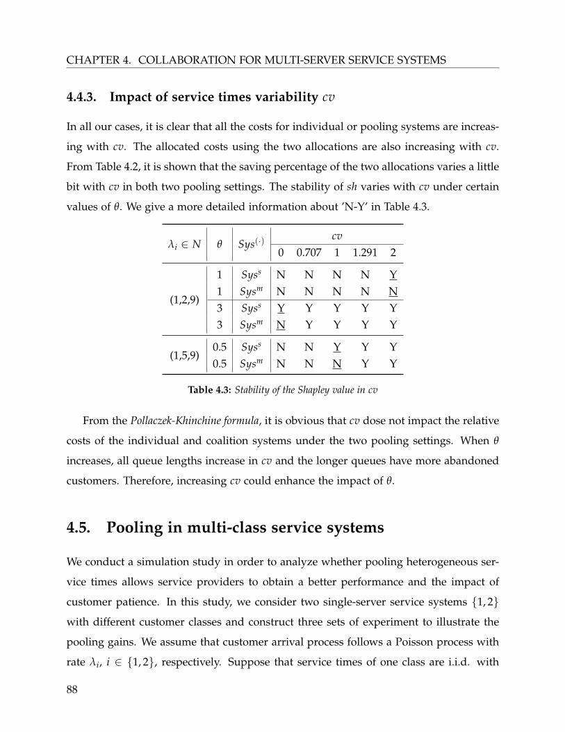
CHAPTER 4. COLLABORATION FOR MULTI-SERVER SERVICE SYSTEMS
4.4.3. Impact of service times variability cv
In all our cases, it is clear that all the costs for individual or pooling systems are increas-
ing with cv. The allocated costs using the two allocations are also increasing with cv.
From Table 4.2, it is shown that the saving percentage of the two allocations varies a little
bit with cv in both two pooling settings. The stability of sh varies with cv under certain
values of θ. We give a more detailed information about ’N-Y’ in Table 4.3.
λi ∈ N θ Sys(·)cv
0 0.707 1 1.291 2
(1,2,9)
1 Syss N N N N Y1 Sysm N N N N N3 Syss Y Y Y Y Y3 Sysm N Y Y Y Y
(1,5,9)0.5 Syss N N Y Y Y0.5 Sysm N N N Y Y
Table 4.3: Stability of the Shapley value in cv
From the Pollaczek-Khinchine formula, it is obvious that cv dose not impact the relative
costs of the individual and coalition systems under the two pooling settings. When θ
increases, all queue lengths increase in cv and the longer queues have more abandoned
customers. Therefore, increasing cv could enhance the impact of θ.
4.5. Pooling in multi-class service systems
We conduct a simulation study in order to analyze whether pooling heterogeneous ser-
vice times allows service providers to obtain a better performance and the impact of
customer patience. In this study, we consider two single-server service systems {1, 2}
with different customer classes and construct three sets of experiment to illustrate the
pooling gains. We assume that customer arrival process follows a Poisson process with
rate λi, i ∈ {1, 2}, respectively. Suppose that service times of one class are i.i.d. with
88

4.5. POOLING IN MULTI-CLASS SERVICE SYSTEMS
mean µ−1i , i ∈ {1, 2} and not change in the pooling system. In the pooling setting, the
two classes have the same priority and are served under FCFS discipline using two i-
dentical parallel servers. When customers are impatient, we assume that the two classes
have an identical abandonment rate θ = 1.
In each set, we consider three cases for the relationship between µ1 and µ2, i.e.,
µ2 = pmcµ1, pmc = {2, 5, 10}, which means that the first class generally gets a longer
service time than the second one. We choose the relative reduction of queue length for
each class and the overall service system to evaluate the pooling performance by using
the following expression,
RLq =
Lq,i−Lp
q,iLq,i
, for class i ∈ {1, 2}∑ Lq,i−Lq
∑ Lq,i, for pooling i ∈ {1, 2}
(4.6)
Firstly, we consider two classes of customers with same server utilization and without
customer abandonment. Our first set of experiments consists of twelve cases with four
values of server utilisation. We consider ρ1 = {0.2, 0.4, 0.6, 0.8} with θ = 0. The values
of pooling gains, noted by RLq, in these twelve cases are given in Table 4.4. We find that
customers of class 1 get more service quality improvement than those of class 2. When
the class heterogeneity pmc increases, the relative pooling performance RLq of class 2 and
overall system {1, 2} decrease. On the contrary, RLq of class 1 increases. This is because
as pmc increases, service times of class 2 are much shorter than those of class 1. Thus, the
congestion impact in the pooling system for each other is much important for class 2.
For a same pmc, RLq decreases with utilizations ρ1 = ρ2. It is also the effect of congestion.
Secondly, we consider different initial utilisations ρi = λi/µi with ρ2 = pduρ1, pdu =
{1/2, 3/2} in Table 4.4. Thus, there are also twelve cases with different server utilisations
considering two values of utilization in class 1, ρ1 = {0.2, 0.6}. Considering the relative
results in Table 4.4 , we could conclude that the relative gains of class 2 increases with
customer arrivals augmentation in this class. Simultaneously, the relative gains of class 1
reduces with additional incoming customers of class 2. It is because that the heavy load
89

CHAPTER 4. COLLABORATION FOR MULTI-SERVER SERVICE SYSTEMS
ρ1 pmc = 2 pmc = 5 pmc = 10C-1 C-2 All C-1 C-2 All C-1 C-2 All
0.2 88.00% 77.40% 82.70% 91.20% 61.60% 76.40% 94.20% 37.40% 65.80%0.4 78.10% 57.44% 67.77% 86.46% 32.20% 59.33% 84.40% −39.09% 22.66%0.6 75.06% 46.92% 60.99% 80.00% 4.86% 42.43% 80.46% −92.24% −5.89%0.8 70.74% 41.11% 55.93% 73.93% −28.98% 22.47% 76.40% −134.66% −29.13%
Table 4.4: Relative pooling performance of two classes of customers with same utilisation and θ = 0
impact on class 2 in individual setting is reduced with the joining of server {1}.
θ = 0 pmc = 2 pmc = 5 pmc = 10ρ1 pdu C-1 C-2 All C-1 C-2 All C-1 C-2 All
0.2 1/2 95.80% 66.70% 90.51% 94.80% 50.50% 86.75% 96.00% −5.30% 77.58%- 3/2 81.60% 79.47% 80.06% 86.40% 67.10% 72.50% 91.20% 46.33% 58.90%
0.6 1/2 84.12% −15.97% 71.61% 89.58% −85.97% 67.63% 90.94% −234.37% 50.28%- 3/2 45.89% 81.60% 78.03% 57.02% 64.78% 64.01% 65.31% 41.29% 43.69%
Table 4.5: Relative pooling performance of two classes of customers with pdu = {1/2, 3/2} and θ = 0
Lastly, we consider the impact of customer impatience in Tables 4.6 and 4.7. The set
of experiments consists of twelve cases with abandonment rate θ = {0.5, 1} and identical
settings for other parameters. It is shown that the impact of customer heterogeneity pmc
still reduces the overall pooling gains and increases the difference of the relative gains
between classes. However, comparing the relative performance under different θ, we
find that the impact of θ weaken the impact of pmc. The negative individual RLq of class
2, caused by class heterogeneity, is reduced with the presence of θ.
Based on above discussions, we could conclude that the service pooling in multi-class
systems is not always profitable owing to the high heterogeneity of classes and the high
system utilization, which is also shown in real-life systems [Vanberkel et al., 2012].
90

4.6. CONCLUSION
θ = 1 pmc = 2 pmc = 5 pmc = 10ρ1 pdu C-1 C-2 All C-1 C-2 All C-1 C-2 All
0.2 1/2 89.44% 81.54% 87.35% 90.00% 38.96% 74.71% 92.78% 23.40% 68.98%- 3/2 70.56% 71.85% 71.54% 82.22% 68.28% 70.63% 85.56% 57.03% 61.45%
0.6 1/2 70.49% 26.22% 57.78% 69.79% −11.59% 38.46% 71.62% −101.02% 1.04%- 3/2 28.59% 41.01% 38.29% 39.58% 35.72% 36.21% 50.85% 26.51% 28.69%
Table 4.6: Relative pooling performance of two classes of customers with pdu = {1/2, 3/2} and θ = {1}
θ = 0.5 pmc = 2 pmc = 5 pmc = 10ρ1 pdu C-1 C-2 All C-1 C-2 All C-1 C-2 All
0.7 1/2 65.55% 11.46% 50.99% 69.60% −56.03% 28.98% 73.76% −133.23% 1.22%- 3/2 23.32% 38.78% 35.58% 40.72% 37.63% 38.01% 44.50% 25.41% 26.97%
0.9 1/2 65.46% −4.64% 47.63% 67.17% −71.98% 21.78% 67.99% −183.82% −22.83%- 3/2 15.72% 31.38% 28.04% 24.48% 28.36% 27.92% 27.24% 24.76% 24.92%
θ = 1 C-1 C-2 All C-1 C-2 All C-1 C-2 All
0.7 1/2 62.41% 10.00% 47.12% 66.48% −32.26% 29.42% 70.96% −97.27% 0.24%- 3/2 31.03% 41.07% 38.84% 40.59% 33.72% 34.61% 46.49% 26.23% 27.94%
0.9 1/2 57.99% 3.38% 41.45% 60.76% −44.51% 18.81% 63.41% −124.20% −21.62%- 3/2 18.98% 30.97% 28.34% 25.34% 25.87% 25.80% 33.01% 24.75% 25.32%
Table 4.7: Relative pooling performance of two classes of customers with high utilisations ρ1 = {0.7, 0.9}
4.6. Conclusion
We considered the service resource pooling problem while accounting for the impor-
tant feature of customer abandonment, and investigated the cooperative strategy among
independent service providers in both the ’super-server’ pooling setting and the multi-
server pooling setting. We assumed that all individual servers are identical and ’super-
server’ is u (the number of servers in the coalition) times faster than the individual
one. With markovian service distributions, we provided a brief analysis for the expected
queue length (related to the abandonment probability) and the expected number of cus-
91

CHAPTER 4. COLLABORATION FOR MULTI-SERVER SERVICE SYSTEMS
tomers in the system. Numerical experiments showed the similar impacts of the service
variability and the customer abandonment on the cost allocations of the two games.
Under the multi-server assumptions, we numerically tested the resource pooling per-
formance in terms of the expected queue length in a 2-class service system. With system
congestion and heterogeneity of classes, the class with faster service is less qualified than
before. When customers are impatient, this individual quality reduction is weakened.
92

Chapter 5
Conclusion and Perspectives
We formulated resource pooling games for three different service models and derived
structure properties under the point of view of cooperation. Using cooperative game
theory, we studied cooperative strategies among a set of independent service providers.
Our approach consists of addressing two consecutive questions: 1) which coalition strat-
egy should be used? and 2) which allocation rule should be selected in order to maintain
the stability of the coalition?
In Chapter 2, we investigated the service pooling game for M/GI/1 service systems.
When service capacities are fixed, we proved that the stable cost allocations always exist
for the grand coalition. When service capacities are optimized to minimize the total
operating costs, we analyzed the properties related to the optimal service rate. We
presented a combined allocation policy in this situation.
In Chapter 3, we extended the pooling problem for service systems while account-
ing for the important feature of customer abandonment. When the service providers
directly combine their queues and service capacities, we proved the existence of stable
allocations. We studied the convexity of the expected queue length in the abandonment
rate and found the special condition of the stability of the Shapley value.
In Chapter 4, we considered the multi-server pooling setting. We investigated nu-
merically the impact of service duration variability and customer abandonment on the
pooling game. We compared between cost-sharing results of the two resource pool-
93
CHAPTER 5. CONCLUSION AND PERSPECTIVES
ing concepts, with or without the ’super-server’ assumptions. Finally, we analyzed the
pooling of two-class service systems.
The results obtained in this Ph.D. thesis provide avenues for futures research. We
next highlight some of them.
Concerning the work of Chapter 1, it would be interesting to extend the analysis to
the cases where the parameters ch, cw or/and f depends on the service provider. For
instance, consider the case of several hospital departments with a shared ward of beds.
The cost of providing medical services by these departments may vary in a great deal,
depending on the medical equipment as well as the medication. Furthermore, the cost
of waiting for a bed may also be significantly different for patients that visit different
departments. Our difficulty with different ch,i is how to define a reasonable pooling ch,S,
especially for the case of optimized service capacity. It is not appropriate to just use
the average of the individual costs ch,S = ∑S ch,iµi/ ∑S µi. We could also use different
cw to define multiple customer classes in the pooling system. The grand coalition may
not be the most profitable coalition under FCFS discipline, because of the increased
expected waiting time for some service providers. Thus, the coalition formation should
be investigated in the service pooling game.
As for the work of Chapter 2, co-opetition is one interesting extensible strategy. Cus-
tomers of a service provider would not be attracted by other providers which are mem-
bers in the coalition under the cooperative point of view. In a co-opetition setting, it is
reasonable to define the service arrival rate as a function of the service performance, i.e.,
the expected waiting time in the system. The co-opetitive strategies could be deduced
from two consecutive problems: 1) how to define the customer arrival rates in function
of system performances? and 2) the pooling strategy is profitable or not?
Concerning the work of Chapter 3, it would be interesting to develop structural re-
sults for the pooling game in order to develop further generic guidelines and insights.
It is important to further study the pooling strategy with multiple customer classes,
which may model for instance a situation with multiple hospital patient types. The ser-
vice times, which is presented as the treatment times, are different in different patient
94

conditions. The characteristics of customer classes could also be described by different
patience times, abandonment costs or waiting costs.
In addition to complex operations and human factors, services are also characterised
by a high impact of advanced technologies. There are many interesting research ques-
tions related to the assessment of the impact of new technologies on customer behavior.
For instance, smart phone apps with delay information, multichannel communication
(email, chat...) with customers. It would be interesting to study the impact of these
features on collaboration strategies.
95

CHAPTER 5. CONCLUSION AND PERSPECTIVES
96

Appendix
Appendix of Chapter 2
Appendix A
Further numerical examples for Section 2.5.4
Further cases related to Table 2.6 are considered here. We vary the number of service
companies from 6 to 15 by adding new service providers in the order of the company
numbers. We study the impact of coalition growing.
Figures F.1 and F.2 provide the cost allocations obtained by the two allocation rules.
We observe that the two allocation methods provide similar solutions. The proportional
allocation shares the pooling cost depending on λi, which is appropriate for an individ-
ual provider. Also, the C∗d reduction depends on λi (Lemma 2.3). Since the Shapley value
is calculated as a function of the contributions of each company, this leads to a similarity
between the two allocations.
The impact of a new participant on this gap is illustrated in Figure F.3. The gap
(absolute difference) between the two allocations for the initial coalition is defined as
AD = ∑6i=1 |φ
p,λi − shopt
i |, for all cases. We find that AD decreases when a new company
joins the coalition for the first three cases. The larger the size of the new company is, the
higher is the reduction of AD. Thus, shopt becomes more and more similar to φp,λ with
scale expansion of the coalition. For the last two cases, we select the initial coalition S6,
which consists of the relatively large or small companies in the set of N = {1, · · · , 15}.
97

APPENDIX
Figure F.1: Proportional allocation cost and Shapley value for the game (N, Copt) of 6 players with f = 0.2
We find that the joining of a small company increases AD for the coalition of relatively
large companies, and the opposite is also true. However, AD decreases or the increase
98

Figure F.2: Proportional allocation cost and Shapley value for the game (N, Copt) of 6 players with f = 1
will reduce when enough companies join the coalition, and AD is relatively small for
the distributed operating costs of S6 (AD/ ∑i∈S6φ
p,λi = 0.5 − 2.5% for all 5 cases).
99
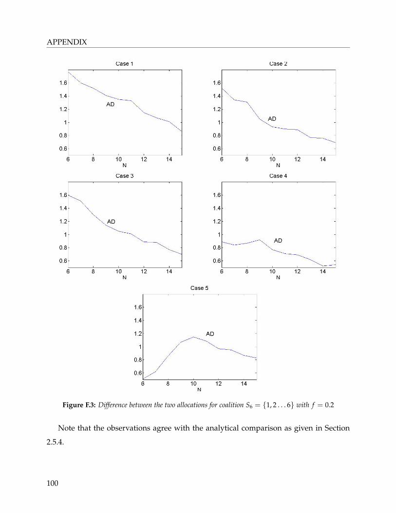
APPENDIX
Figure F.3: Difference between the two allocations for coalition S6 = {1, 2 . . . 6} with f = 0.2
Note that the observations agree with the analytical comparison as given in Section
2.5.4.
100

Appendix of Chapter 3
Appendix B
Numerical illustrations with impatience
For cases with more than 3 players, we consider three typical examples as in [Peng
et al., 2015], with low, high and very different offered loads. From Table F.1, we observe
that the interval Θ = ∅ also exists. By comparing the offered loads ρ0(i) = λi/µi and Θ,
it can be seen that the two bounds of Θ are related to the coefficient of variation (c.v.) of
ρ0.
System data Customer arrival rates Offered load ρ0
µ θlow θup No. 1 2 3 4 5 6 mean c.v.
10 0.56 5769.86 1 2 3 3 4 3.5 4 0.3250 0.2333
- 0.04 32048.84 2 7 9 8 7 8.5 9.5 0.8167 0.1265
- 1.83 1584.23 3 2 7 4 7.5 9 3 0.5416 0.5170
Table F.1: System parameters and offered loads of 6 players games
For a more detailed analysis of Θ, we randomly choose the values of the two variables
λi and µi in (0, 10) (without the constraint of λi < µi) and search the stable interval of
sh f ix with n ∈ {3, ..., 10}. In the 3 players games as shown in Table F.2, it is interesting to
see that the interval width Θ is narrowed with the increase of the coefficient of variation
(c.v.) of ρ0 for the cases (fourth to tenth lines) in which sh f ix is not stable in θ = 0 and
θ → +∞ situations.
We test 1000 random cases of n players games for 10 times, respectively with n ∈
{3, ..., 10}. Again, we randomly choose the values of λi and µi in (0, 10) for each random
event. From the numerical results, we find out some cases with |Θ| = 0, i.e., there is no
θ ∈ R+ with sh f ix staying in the core. As shown in Fig. F.4, the probability of |Θ| = 0 in
1000 cases is negligible for n = 3 (it is 0.8 − 1.4%) and it increases in n. When n = 10,
this probability reaches 5.9 − 8.4%.
101
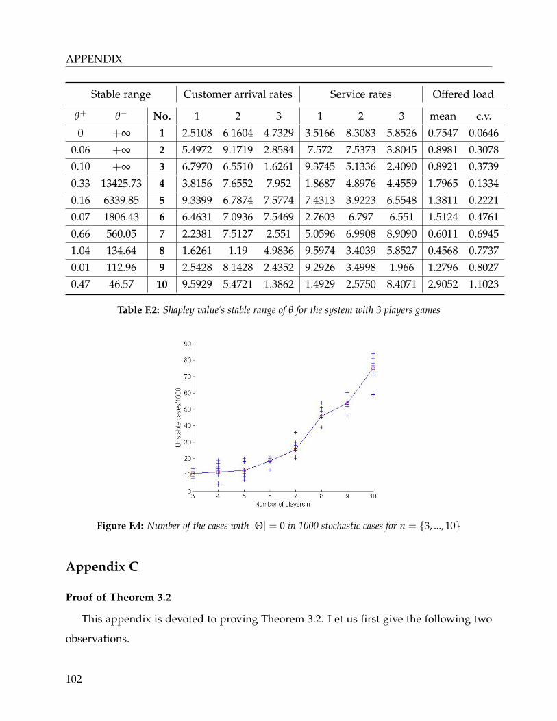
APPENDIX
Stable range Customer arrival rates Service rates Offered load
θ+ θ− No. 1 2 3 1 2 3 mean c.v.
0 +∞ 1 2.5108 6.1604 4.7329 3.5166 8.3083 5.8526 0.7547 0.0646
0.06 +∞ 2 5.4972 9.1719 2.8584 7.572 7.5373 3.8045 0.8981 0.3078
0.10 +∞ 3 6.7970 6.5510 1.6261 9.3745 5.1336 2.4090 0.8921 0.3739
0.33 13425.73 4 3.8156 7.6552 7.952 1.8687 4.8976 4.4559 1.7965 0.1334
0.16 6339.85 5 9.3399 6.7874 7.5774 7.4313 3.9223 6.5548 1.3811 0.2221
0.07 1806.43 6 6.4631 7.0936 7.5469 2.7603 6.797 6.551 1.5124 0.4761
0.66 560.05 7 2.2381 7.5127 2.551 5.0596 6.9908 8.9090 0.6011 0.6945
1.04 134.64 8 1.6261 1.19 4.9836 9.5974 3.4039 5.8527 0.4568 0.7737
0.01 112.96 9 2.5428 8.1428 2.4352 9.2926 3.4998 1.966 1.2796 0.8027
0.47 46.57 10 9.5929 5.4721 1.3862 1.4929 2.5750 8.4071 2.9052 1.1023
Table F.2: Shapley value’s stable range of θ for the system with 3 players games
Figure F.4: Number of the cases with |Θ| = 0 in 1000 stochastic cases for n = {3, ..., 10}
Appendix C
Proof of Theorem 3.2
This appendix is devoted to proving Theorem 3.2. Let us first give the following two
observations.
102

Observation F.1. For ai, bi ∈ R+ (i ∈ {1, 2, 3, 4}), assume that a1 + a4 = a2 + a3 with
0 ≤ a1 ≤ a2 ≤ a3 ≤ a4, and b1 + b4 ≤ b2 + b3 with b1 ≥ max{b2, b3, b4}. Then, a1b1 +
a4b4 ≤ a2b2 + a3b3.
Proof. We define b4 = b2 + b3 − b1, such that b1 + b4 ≤ b1 + b4 = b2 + b3. Thus, b4 ≥ b4.
This implies a1b1 + a4b4 ≤ a1b1 + a4b4 ≤ a2b1 + a3b4 ≤ a2b2 + a3b3, which finishes the
proof of the observation.
Observation F.2. For ai, bi ∈ R+ (i ∈ {1, 2, 3, 4}), assume that a1 + a4 = a2 + a3 with
0 ≤ a1 ≤ a2 ≤ a3 ≤ a4, and b1 + b4 ≤ b2 + b3 with b1 ≥ max{b2, b3, b4}. If a1b1 ≥
max{a2b2, a3b3, a4b4}, then a4b4 ≤ min{a1b1, a2b2, a3b3} and vice versa.
Proof. We define b4 = b2 + b3 − b1 ≥ b4. We assume that a2 − a1 = a, a3 − a2 = △a and
b1 − max{b2, b3} = b, | b2 − b3 |= △b. If b2 ≥ b3, we have
a2b2 = a1b1 + A,
a3b3 = a1b1 + A + B,
a4b4 ≤ a4b4 = a1b1 + 2A + B − C,
with A = aa1 −△aa1 − ab, B = △a(a1 − a)−△b(b1 + b)−△a △ b and C = 2ab +△aa +
△bb. Since a1b1 ≥ max{a2b2, a3b3, a4b4}, we obtain A ≤ 0, A + B ≤ 0 and C ≥ 0.
Thus, a4b4 ≤ min{a1b1, a2b2, a3b3}. Similarly, we could prove the same result in the case
of b2 < b3. When a4b4 ≥ max{a1b1, a2b2, a3b3}, we define b1 = b2 + b3 − b4 such that
b1 ≥ b1. We then obtain a1b1 ≤ min{a2b2, a3b3, a4b4} from the symmetry of ai and bi,
which completes the proof of this observation.
We now proceed to the concavity proof of the queue length.
Proof. of Theorem 2. We define the same Y, X(θ) and X+(θ) as in the proof of Lemma
3.1. The decreasing property in θ ∈ (0,+ inf) is easy to get from the transition rate of Y,
λ/(µ + jθ), which is decreasing in θ. Following similar arguments as for Lemma 3.1, we
can prove this theorem by proving that X is SDCX(sp) in θ if θ ≤ µ. In this proof, we
103

APPENDIX
focus on the SDCX(sp) of X in θ, using a similar method used for that of X in µ in the
proof of Theorem 1 in [Armony et al., 2009].
We use the definition of sample path convexity as defined in [Shaked and Shanthiku-
mar, 1988]. For initialization, we choose four abandonment rates 0 ≤ θ1 ≤ θ2 ≤ θ3 ≤
θ4 ≤ µ with θ1 + θ4 = θ2 + θ3. All the other system parameters λ and µ are held constant.
If X is SDCX(sp), then Xi =st X(θi), i ∈ {1, 2, 3, 4}, defined on the same probability space
as the uniformized Markov process of Xi defined at time m, satisfies
Condition 1. X1(m) + X4(m) ≥ X2(m) + X3(m), a.s.
Condition 2. X1(m) ≥ max{X2(m), X3(m), X4(m)}, a.s., for all m ∈ N.
For uniformization, we define Kθi with K ∈ N+ as the upper limit of the abandon-
ment rate, which means that there are at maximum K customers that has the intention
to abandon the queue at a given time. The maximum transition rate of all Xi is upper
bounded by υ = λ + µ + Kθ4. Thus, we define XKi as the uniformized version of Xi.
Now, we will show that for any K, Conditions 1 and 2 hold for any m ∈ N, then XK is
SDCX(sp). To simplify the presentation, we write XKi as Xi in the following arguments.
The proof of the two conditions is done by induction on the discrete time m. Firstly,
we suppose that the equality of Condition 1, denoted by 1, and Condition 2 hold at time
m. We next build the transition probability to satisfy Conditions 1 and 2 at time m + 1.
With a probability of λ/υ, new customers arrive into all the four systems. The similar
transition definition is used for the service completion, services are completed simulta-
neously in all systems with a probability of µ/υ. Consider a special definition in case of
X4 = 0, which will be discussed later on.
For the abandonment process, there is a probability of min{(Xi − 1)+, K}θi/υ that one
customer abandons from system i, i ∈ {1, 2, 3, 4}. Define X(K)+i = min{(Xi − 1)+, K}.
From the concavity of f = min{x, K}, we have X(K)+1 + X(K)+
4 ≤ X(K)+2 + X(K)+
3 for
the not empty queues (Xi = 0 for all systems). To further specify the abandonment
transition probability for each system, we define four cases depending on the order of
104

X(K)+i θi denoted by ϑi. From Observation F.1, Conditions 1 and 2, it follows
ϑ1 + ϑ4 ≤ ϑ2 + ϑ3, (F.1)
at time m.
Consider the existence of empty queues (Xi = 0 for some systems). According to
Conditions 1 and 2, there are four possible situations: no customer in Systems {1, 2, 3, 4},
{2, 4}, {3, 4} or 4. When Systems {1, 2, 3, 4}, {2, 4} or {3, 4} are empty, Inequality (F.1)
still holds. The only exception happens when System 4 is the only empty system. In
this case, we have ϑ1 + µ ≤ (ϑ2 + µ) + (ϑ3 + µ) with θ4 ≤ µ. Here, we deal with the
service completion and the customer abandonment process together and choose ϑi equal
to ϑi + µ. Thus, Inequality (F.1) holds with ϑ4 = ϑ(4) = 0.
From Observation F.2, the four following cases meet Inequality (F.1). We define ϑ(i)
for i ∈ {1, 2, 3, 4}, such that 0 ≤ ϑ(4) ≤ ϑ(3) ≤ ϑ(2) ≤ ϑ(1). Let a random variable
pa ∼ Uni f orm(0, 1).
Case 1. If ϑ(1) + ϑ(4) ≤ ϑ(2) + ϑ(3). Let ϑ = max{Kθ4, ϑ(2) + ϑ(3) − ϑ(4)}.
• I) If pa ≤ ϑ(4)/ϑ, there are customers abandoning from all systems;
• II) If ϑ(4)/ϑ ≤ pa ≤ ϑ(3)/ϑ, there are customers abandoning from Systems {1, 3};
• III) If ϑ(3)/ϑ ≤ pa ≤ ϑ(1)/ϑ, there are customers abandoning from Systems {1, 2};
• IV) If ϑ(1)/ϑ ≤ pa ≤ (ϑ(2) + ϑ(3) − ϑ(4))/ϑ, there is one customer abandoning from
System 2.
Case 2. If ϑ(2) + ϑ(3) ≤ ϑ(1) + ϑ(4). Let ϑ = max{Kθ4, ϑ(1)}.
• I) If pa ≤ ϑ(4)/ϑ, there are customers abandoning from all systems;
• II) If ϑ(4)/ϑ ≤ pa ≤ ϑ(3)/ϑ, there are customers abandoning from Systems {1, 3};
• III) If ϑ(3)/ϑ ≤ pa ≤ (ϑ(2) + ϑ(3) − ϑ(4))/ϑ, there are customers abandoning from
System {1, 2};
• IV) If (ϑ(2) + ϑ(3) − ϑ(4))/ϑ ≤ pa ≤ ϑ(1)/ϑ, there is one customer abandoning from
System 1.
Case 3. If ϑ(2) + ϑ(4) ≤ ϑ(1) + ϑ(3). Let ϑ = max{Kθ4, ϑ(1)}.
105

APPENDIX
• I) If pa ≤ ϑ(4)/ϑ, there are customers abandoning from all systems;
• II) If ϑ(4)/ϑ ≤ pa ≤ ϑ(3)/ϑ, there are customers abandoning from Systems {1, 2, 3};
• III) If ϑ(3)/ϑ ≤ pa ≤ ϑ(2)/ϑ, there are customers abandoning from Systems {1, 2};
• IV) If ϑ(2)/ϑ ≤ pa ≤ ϑ(1)/ϑ, there is one customer abandoning from System 1;
Case 4. If ϑ(3) + ϑ(4) ≤ ϑ(1) + ϑ(2). Let ϑ = max{Kθ4, ϑ(1) + ϑ(2) − ϑ(3)}.
• I) If pa ≤ ϑ(4)/ϑ, there are customers abandoning from all systems;
• II) If ϑ(4)/ϑ ≤ pa ≤ ϑ(3)/ϑ, there are customers abandoning from Systems {1, 2, 3};
• III) If ϑ(3)/ϑ ≤ pa ≤ ϑ(1)/ϑ, there is one customer abandoning from System 1;
• IV) If ϑ(1)/ϑ ≤ pa ≤ (ϑ(1) + ϑ(2) − ϑ(3))/ϑ, there is one customer abandoning from
System 2;
We next show that if Conditions 1 and 2 hold at time m, then Conditions 1 and 2 hold
at time m + 1.
For the arrival process, it is obvious that Conditions 1 and 2 hold at m + 1. From
Condition 2, service completions from the left hand side of Condition 1 are not higher
than those from the other hand side, and X1 stays as the longest queue. This is because
service completions 1) happen in both systems if X2 = X1 or X3 = X1; 2) happen
in the three systems or all systems if X2 = X3 = X1; 3) happen in all systems if all
queue lengths are identical. For the abandonment process, it is clear that the number of
abandoned customers in Systems {1, 4} is not higher than that in Systems {2, 3} after
one step transition in the case of X(K)+i > 0, i.e., Inequality (F.1) holds for all the four
cases. Now, we discuss special situations in the customer abandonment process.
• I) All the four queues X(K)+i are empty, there is no abandonment in all systems;
• II) If two queues ({2, 4} or {3, 4}) are empty, we have ϑ(2) ≤ ϑ(1) corresponding to
Case 2. System 1 has an abandonment only if System 2 does;
• III) If X+4 = 0, System 1 has an abandonment when at least one customer abandons
in the System 2 or 3 (in Case 1, 3 or 4);
Thus, Condition 1 holds in the abandonment process at time m + 1. For Condition 2, we
have
106

• I) If X1(m) > max{X2(m), X3(m), X4(m)}, it is obvious that Condition 2 holds at
time m + 1;
• II) If ϑ1 = ϑ(4), a customer abandons from System 1 when customers have aban-
doned from all the other 3 systems;
• III) If ϑ1 = ϑ(3) with X1 = X2 > X4 (or X1 = X3 > X4) and X3 = X4 (or X2 = X4),
we have ϑ2 ≥ ϑ1 and ϑ4 ≥ ϑ3. Then, ϑ4 = ϑ(4). The corresponding case is Case 2.
and we have ϑ2 = ϑ(1). Customers abandon from Systems {1, 2} together;
• IV) If ϑ1 = ϑ(2) with X1 = X2 > X4 (or X1 = X3 > X4), we have ϑ2 = ϑ(1) ≥ ϑ1 . In
the corresponding cases (Cases 2 and 3), a customer abandons from System 1 only
if a customer has abandoned from System 2;
• V) If X1(m) = X2(m) = X3(m) = X4(m), we have 0 ≤ ϑ1 ≤ ϑ2 ≤ ϑ3 ≤ ϑ4, which
coincides with Case 1 and X1 = ϑ(4).
As summary in the above paragraphs, it is shown that if Conditions 1 and 2 hold
at time m, Conditions 1 and 2 hold at time m + 1. If strict inequality of Condition 1
holds, we define X4(m) = max{0, X2(m) + X3(m) − X1(m)} ≤ X4(m) and X1(m) =
min{X2(m) + X3(m), X1(m)} ≤ X1(m). It means that if X2 + X3 − X1 ≥ 0, we decrease
X4 = X2 + X3 − X1 ≥ 0 and keep X1 = X1. We have X1 = X2 + X3 and X4 = 0 in the
opposite case. We have X1(m)+ X4(m) = X2(m)+X3(m). Then, Conditions 1 and 2 hold
for {X1, X2, X3, X4} at time m + 1. For each θi, we denote the complementary cumulative
distribution function (ccdf) by Fθi(y; x) = Pθi{X(m + 1) > y|X(m) = x} and its inverse
Fθi(v; x)−1 = in f {y : Fθi(y; x) ≤ v}, v ∈ [0, 1]. Define Xi(m + 1) = F−1θi
(Fθi(Xi(m +
1); Xi(m)); Xi(m)) for i = {1, 4}. From the transition probabilities determined in the
previous paragraphs, it follows that Fθi(y; x) is non-decreasing in x. Thus, (Xi(m +
1) − Xi(m)) ≥ (Xi(m + 1) − Xi(m)) for i = {1, 4} and Conditions 1 and 2 hold for
{X1, X2, X3, X4} at time m + 1 with the corresponding transition probabilities. The proof
of Conditions 1 and 2 for XK is now completed. Therefore, E(XK) is decreasing and
convex in θ. Since XK(θ)st−−−−→
K−→∞X(θ) for each θ ∈ [0, µ], E(X) is decreasing and convex
in θ from Proposition 2.11 in [Shaked and Shanthikumar, 1988]. The proof of the theorem
is completed.
107

APPENDIX
108
Appendix D Résumé étendu
1. Introduction & motivation
Le secteur des services est devenu le secteur le plus important en nombre d’emplois
occupés dans l’économie mondiale (figure 1.1, page 6), en particulier dans les pays
développés, les services représentent jusqu’à 70% de la production nationale (PIB) et
sont devenus leur principal moteur de croissance économique. Par exemples, quatre sur
cinque emplois aux Etats-Unis sont fournis par le secteur de services ; le secteur tertiaire
français occupait 76,8% de la population active en 2015.
Beaucoup de nos activités quotidiennes dépendent des services et des fournisseurs
de services, de l’e-mail que nous vérifions le matin au service de transport public que
nous prenons pour aller à notre lieu de travail, du restaurant dans lequel nous déjeunons
à midi au colis que nous recevons pendant la journée. Les services sont partout dans
notre vie, y compris dans les domaines de la finance (banques, stocks), la santé (médecin
personnel, hôpital), la communication (courrier électronique, réseau 4G), les services
publics (électricité, police), etc. [Daskin, 2010]
Dans le contexte de la mondialisation économique, la concurrence et la coopération
dans les industries de services sont devenues de plus en plus communes: la concur-
rence des prix entre les chaînes de restauration rapide, le regroupement des entreprises
de télécommunication, les services collaboratifs d’après-vente et de maintenance dans
l’industrie électronique, pour n’en citer que quelques-uns. Dans cette thèse, nous étu-
dions des stratégies collaboratives dans les systèmes de service homogènes. Nous nous
concentrons en particulier sur les stratégies de pooling des ressources. Notre approche
consiste à utiliser la modélisation des systèmes de service par les files d’attents et la
théorie des jeux pour l’analyse des interactions entre les fournisseurs de services. Dans
ce qui suit, nous discutons brièvement les stratégies de collaboration et de pooling des
ressources.
109

APPENDIX
Stratégies collaboratives dans les services
Afin d’améliorer les performances du système ou de réduire les dépenses, il existe
plusieurs méthodes coopératives basiques: la coopération entre les files d’attente, par
exemple, la dispatching d’arrivée simultanées entre les agences ou le réacheminement
entre des serveurs différents [Katta and Sethuraman, 2006, Kayi and Ramaekers, 2010];
le pooling des services, p.ex., le pooling des capacités de service ou la répartition en
personnel [Guo et al., 2013]; le cross-training [Tekin et al., 2014]; la collaboration avec
des fournisseurs tiers, par exemple l’externalisation de services [Aksin et al., 2008], etc.
Il est parfois utile de combiner ces méthodes pour aboutir à une structure collaborative
plus rentable [Anily and Haviv, 2014].
Les méthodes de coopération pourrait être classées sous trois formes typiques (fig-
ure 1.2, page 8): la forme verticale, les collaborations entre les différents éléments du
système, par exemple, les forfaits de téléphone portable signé par les clients avec les
opérateurs télécoms, les cartes annuelles d’accès au club de sport; la forme horizon-
tale, la collaboration entre les serveurs homogènes, par ex., les services après-vente de
produits électroniques de différentes marques; et les externalisations, la collaboration
avec une partie tiers aux systèmes de service, par exemple, le service client sous-traité à
l’étranger.
Parmi la majorité des gains réalisée par les activités collaboratives, la réduction des
coûts est le facteur le plus important pour les fournisseurs de services. Le coût de la ca-
pacité de service et le coût d’attente des clients dans la file d’attente ou le système sont
largement utilisés dans la littérature [Anily and Haviv, 2010, Özen et al., 2011, Karsten
et al., 2015b, Yu et al., 2015].
Pooling des ressources
Depuis la première étude de [Stidham, 1970], le pooling des systèmes de file d’attente
a été largement étudié dans la littérature pour la conception des systèmes de service.
110

Il est bien connu que le pooling de la capacité de service amène naturellement à des é-
conomies d’échelle dans les études de gestion opérationnelle [Smith and Whitt, 1981, Bell
and Williams, 2005]. Cette amélioration de l’efficacité opérationnelle est générée par la
disparition des ressources de service libres dans le système quand il est en présence de
congestion dans les files d’attente. Ceci est valide à la fois dans le cas de départements
d’une même entité économique, comme par exemple, le pooling des réservations dans
un restaurant [Thompson and Kwortnik, 2008], ou dans le cas de plusieurs entités in-
dépendantes [González and Herrero, 2004, Garcia-Sanz et al., 2008, Anily and Haviv,
2010, Kayi and Ramaekers, 2010, Tekin et al., 2014, Anily and Haviv, 2014].
Les applications en pratique pour le pooling des services parmi les fournisseurs de
services homogènes sont nombreuses. Par exemple, les différents départements d’un
hôpital peuvent partager une salle d’opération commune afin de réduire les dépens-
es. Ils pourraient également partager leur capacité en termes de lits dans les chambres
d’hôpital, ce qui permettrait de soulager la congestion. Un autre exemple est dans le
contexte de service après-vente pour certaines catégories de produits électroniques. Ces
produits sont susceptibles d’avoir un faible taux de demande après-vente pour chaque
détaillant individuellement. En conséquence, les détaillants pourraient fournir un ser-
vice après-vente conjoint pour réduire les coûts de démarrage du service et améliorer
la qualité du service. Pour les services d’aviation, le service d’enregistrement en com-
mun pour différentes compagnies aériennes est un exemple supplémentaire pour les
applications du pooling d’ensemble services.
Parmi les perspectives de recherche, on peut définir les stratégies de pooling des
ressources plus précisé. Selon les participants, on peut distinguer les cas des différentes
branches d’une même entité économique [Alptekinoglu et al., 2013] ou de plusieurs en-
tités indépendantes [Anily and Haviv, 2014]; Selon les méthodes de pooling, on peut dis-
tinguer les cas avec pooling des ressources partiel [Chao et al., 2003] ou complète [Anily
and Haviv, 2010]; Selon la définition de la valeur des systèmes issue de la théorie des
jeux, on peut distinguer les cas avec la valeur transférable ou la valeur non-transférable,
par exemples, le coût, est une valeur transférable [Karsten et al., 2015b], et la réputation
111

APPENDIX
de fournisseur est non-transférable [Toivonen, 2014]. Dans cette thèse, nous travaillons
sur les stratégies du pooling des ressources complètes entre plusieurs entités indépen-
dantes, et la valeur des systèmes est mesurée par les coûts globaux.
Il existe des similitudes entre le management opérationnelle de service et de biens
manufacturés, tous les deux sont concernés par l’efficience, l’efficacité, les problèmes de
qualité et motivés par la réduction des coûts. Contrairement à l’existence de travaux de
recherche dans l’industrie manufacturière, les recherches relatifs à l’industrie de service
ne répendant pas aux exigences de son développement économique énorme.
Les services sont principalement caractérisés par des opérations complexes et un im-
pact élevé des facteurs humains. Dans cette thèse, nous tenons compte de ces deux
aspects par l’analyse de l’impact de la variabilité de la durée du service et de l’abandon
du client, respectivement. Nous étudions le problème dans lequel les fournisseurs de
service indépendants pourraient être amenés à coopérer entre eux. Nous considérons la
stratégie de pooling des ressources dans différents systèmes de services et fournissons
des stratégies de pooling correspondantes en utilisant la théorie des jeux coopératifs.
2. Objectif & contributions
L’objectif de cette thèse est d’étudier l’impact des caractéristiques de la variabilité des
services et de l’abandon des clients sur les stratégies de collaboration. Motivés par la
réduction des coûts, nous traitons le problème de pooling des ressources entre les four-
nisseurs de services indépendants. Nous utilisons la théorie des files d’attente pour la
modélisation de ces caractéristiques. Plus concrètement, nous posons les deux ques-
tions suivantes: 1) comment former les coalitions? Et 2) quelle règle d’allocation doit
être choisie pour garantir la stabilité de la coalition? Nous utilisons la théorie des jeux
coopératifs, qui fournit des concepts intéressants pour analyser les structures de coali-
tions profitables et résoudre le problème de partage des coûts entre les participants.
Les principales contributions de cette thèse peuvent être résumées comme suit.
Premièrement, nous étudions le problème du partage des coûts entre les fournisseurs
112

de services indépendants dans le cadre d’un système de pooling des capacités de service
avec des temps de service distribués suivant une loi générale. L’amélioration effective est
obtenue en réduisant les ressources inutilisées en cas de congestion. Nous modélisons
à la fois le fournisseur de services et la coalition coopérative par des files d’attente
à un seul serveur avec des délais de service suivant une loi générale. Pour les deux
situations de pooling avec une capacité de service fixe et de pooling avec une capacité
de service optimisée, nous définissons les jeux coopératifs correspondants et analysons
les allocations du cœur du jeu. Pour le cas avec capacité fixe, nous prouvons que le
cœur est non vide. La fonction caractéristique n’est ni concave ni monotone dans le
jeu mentionné. Cependant, nous prouvons que le jeu de pooling de service avec la
capacité de service optimisée est concave. Pour ce jeu concave, nous trouvons deux
règles d’allocation stables et illustrons une stratégie combinée d’allocation des coûts.
Deuxièmement, nous considérons un groupe de fournisseurs de service homogènes
et indépendants, où un client quitte le système sans service chaque fois que son attente
dans la file d’attente dépasse son seuil de temps de patience. L’avantage de la collabo-
ration dans ces systèmes avec l’abandon des clients, n’est pas seulement le partage de
ressources instantanées disponibles, mais aussi la réduction des clients qui abandonnen-
t. Selon les hypothèses markoviennes sur les temps d’arrivée, de service et de patience,
nous définissons un jeu coopératif avec utilité transférable et une capacité de service fixe
pour chaque individu et chaque coalition. Nous prouvons que la grande coalition est la
coalition la plus profitable et que le jeu a un cœur non vide. Nous examinons ensuite
l’impact de l’abandon sur la stabilité de la valeur de Shapley. De plus, nous démontrons
la concavité de la longueur de la file d’attente en fonction du taux d’abandon et donnons
une condition selon laquelle la valeur Shapley est située dans le cœur. Nous étudions
également le problème de partage des coûts du jeu coopératif relatif avec la capacité de
service optimisée et prouvons que la règle d’allocation proportionnelle selon les taux
d’arrivée des clients donne une allocation stable dynamique à tous les sous-jeux relatifs.
Dans les études précédentes, nous utilisons les hypothèses de ≪ super-serveur ≫.
La raison principale de cette hypothèse est que traiter les systèmes des files d’attente
113

APPENDIX
multiserveurs avec les temps de service distribué selon une loi générale et avec abandon
des clients est très complexe. Pour évaluer la qualité de ces hypothèses, nous étudions
numériquement le problème des stratégies de pooling des services dans le cas multi-
serveurs. Bien qu’il soit intuitif de s’attendre à des améliorations d’efficacité dans les
systèmes de pooling multiserveurs, il n’est pas évident de conclure que tous les mem-
bres bénéficieront du pooling comme c’est le cas pour le ≪ super-serveur ≫. Nous
comparons les deux cadres de pooling et nous évaluons numériquement les effets de la
variabilité des services et de l’abandon des clients dans les deux jeux correspondants.
114

Bibliography
[Aksin et al., 2008] Aksin, O., de Véricourt, F., and Karaesmen, F. (2008). Call center
outsourcing contract analysis and choice. Management Science, 54(2):354–368.
[Alptekinoglu et al., 2013] Alptekinoglu, A., Banerjee, A., Paul, A., and Jain, N. (2013).
Inventory pooling to deliver differentiated service. Manufacturing & Service Operations
Management, 15(1):33–44.
[Andradóttir et al., 2017] Andradóttir, S., Ayhan, H., and Down, D. (2017). Resource
pooling in the presence of failures: Efficiency versus risk. European Journal of Opera-
tional Research, 256:230–241.
[Anily and Haviv, 2007] Anily, S. and Haviv, M. (2007). The cost allocation problem for
the first order interaction joint replenishment model. Operations Research, 55(2):292–
302.
[Anily and Haviv, 2010] Anily, S. and Haviv, M. (2010). Cooperation in service systems.
Operations Research, 58(3):660–673.
[Anily and Haviv, 2014] Anily, S. and Haviv, M. (2014). Subadditive and homogeneous
of degree one games are totally balanced. Operation Research, 62(4):788–793.
[Armony et al., 2009] Armony, M., Plambeck, E., and Seshadri, S. (2009). Sensitivity
of optimal capacity to customer impatience in an unobservable M/M/S queue (why
you shouldn’t shout at the DMV). Manufacturing and Service Operations Management,
11(4):19–32.
115

[Batt and Terwiesch, 2015] Batt, R. and Terwiesch, C. (2015). Waiting patiently: An em-
pirical study of queue abandonment in an emergency department. Management Sci-
ence, 61(1):39–59.
[Bell and Williams, 2005] Bell, S. and Williams, R. (2005). Dynamic scheduling of a par-
allel server system in heavy traffic with complete resource pooling: Asymptotic opti-
mality of a threshold policy. Electronic Journal of Probability, 10(33):1044–1115.
[Benjaafar et al., 2005] Benjaafar, S., Cooper, W., and Kim, J. (2005). On the benefits of
pooling in production-inventory systems. Management Science, 51(4):548–565.
[Bondareva, 1963] Bondareva, O. (1963). Some applications of linear programming
methods to the theory of cooperative games. Problemy Kibernetiki, 10:119–139.
[Chao et al., 2003] Chao, X., Liu, L., and Zheng, S. (2003). Resource allocation in mul-
tisite service systems with intersite customer flows. Management Science, 49(12):1739–
1752.
[Chun, 2006a] Chun, Y. (2006a). No-envy in queueing problems. Economic Theory,
29(1):151–162.
[Chun, 2006b] Chun, Y. (2006b). A pessimistic approach to the queueing problem. Math-
ematical Social Sciences, 51(2):171–181.
[Cruijssen et al., 2007] Cruijssen, F., Cools, M., and Dullaert, W. (2007). Horizontal co-
operation in logistics: opportunities and impediments. Transportation Research Part E:
Logistics and Transportation Review, 43(2):129–142.
[Dai and He, 2010] Dai, J. and He, S. (2010). Customer abandonment in many-server
queues. Mathematics of Operations Research, 35(2):347–362.
[Daskin, 2010] Daskin, M. (2010). Service science, volume 1. Wiley Online Library.
[Dijk and Sluis, 2008] Dijk, N. and Sluis, E. (2008). To pool or not to pool in call centers.
Production and Operations Management, 17(3):296–305.
116

BIBLIOGRAPHY
[Drechsel and Kimms, 2010] Drechsel, J. and Kimms, A. (2010). Computing core alloca-
tions in cooperative games with an application to cooperative procurement. Interna-
tional Journal of Production Economics, 128(1):310–321.
[Driessen, 1988] Driessen, T. S. H. (1988). Cooperative Games, Solutions and Applications.
Kluwer Academic Publishers.
[Dror et al., 2012] Dror, M., Hartman, B., and Chang, W. (2012). The cost allocation issue
in joint replenishment. International Journal of Production Economics, 135(1):242–254.
[Elomri et al., 2012] Elomri, A., Ghaffari, A., Jemai, Z., and Dallery, Y. (2012). Coalition
formation and cost allocation for joint replenishment systems. Production and Opera-
tions Management, 21(6):1015–1027.
[Ferguson, 2014] Ferguson, T. (2014). Mathematical Statistics: A Decision Theoretic Ap-
proach, volume 1. Academic press.
[Fiestras-Janeiro et al., 2013] Fiestras-Janeiro, M., García-Jurado, I., Meca, A., and Mos-
quera, M. (2013). A new cost allocation rule for inventory transportation systems.
Operations Research Letters, 41(5):449–453.
[Frisk et al., 2010] Frisk, M., Göthe-Lundgren, M., Jörnsten, K., and Rönnqvist, M.
(2010). Cost allocation in collaborative forest transportation. European Journal of Oper-
ational Research, 205(2):448–458.
[Garcia-Sanz et al., 2008] Garcia-Sanz, M., Fernández, F., Fiestras-Janeiro, M., García-
Jurado, I., and Puerto, J. (2008). Cooperation in markovian queueing models. European
Journal of Operational Research, 188(2):485–495.
[Garnett et al., 2002] Garnett, O., Mandelbaum, A., and Reiman, M. (2002). Designing a
call center with impatient customers. Manufacturing & Service Operations Management,
4:208–227.
117

[Gerchak and Gupta, 1991] Gerchak, Y. and Gupta, D. (1991). On apportioning costs to
customers in centralized continuous review inventory systems. Journal of Operations
Management, 10(4):546–551.
[Gillies, 1959] Gillies, D. (1959). Solutions to general non-zero-sum games. Contributions
to the Theory of Games, 4(40):47–86.
[González and Herrero, 2004] González, P. and Herrero, C. (2004). Optimal sharing of
surgical costs in the presence of queues. Mathematical Methods of Operations Research,
59(3):435–446.
[Guajardo and Rönnqvist, 2015] Guajardo, M. and Rönnqvist, M. (2015). Cost allocation
in inventory pools of spare parts with service-differentiated demand classes. Interna-
tional Journal of Production Research, 53(1):220–237.
[Guardiola et al., 2009] Guardiola, L., Meca, A., and Puerto, J. (2009). Production-
inventory games: A new class of totally balanced combinatorial optimization games.
Games and Economic Behavior, 65(1):205–219.
[Gunal, 2012] Gunal, M. (2012). A guide for building hospital simulation models. Health
Systems, 1(1):17–25.
[Guo et al., 2013] Guo, P., Leng, M., and Wang, Y. (2013). A fair staff allocation rule for
the capacity pooling of multiple call centers. Operations Research Letters, 41(5):490–493.
[Harrison and López, 1999] Harrison, J. and López, M. (1999). Heavy traffic resource
pooling in parallel-server systems. Queueing Systems, 33(4):339–368.
[Hartman and Dror, 1996] Hartman, B. and Dror, M. (1996). Cost allocation in
continuous-review inventory models. Naval Research Logistics, 43(4):549–561.
[Hartman et al., 2000] Hartman, B., Dror, M., and Shaked, M. (2000). Cores of inventory
centralization games. Games and Economic Behavior, 31(1):26–49.
118

BIBLIOGRAPHY
[Iyer and Jain, 2004] Iyer, A. and Jain, A. (2004). Modeling the impact of merging capac-
ity in production-inventory systems. Management Science, 50(8):1082–1094.
[Jouini, 2012] Jouini, O. (2012). Analysis of a last come first served queueing system
with customer abandonment. Computers & Operations Research, 39:3040–3045.
[Jouini et al., 2008] Jouini, O., Dallery, Y., and Nait-Abdallah, R. (2008). Analysis of the
impact of team-based organizations in call center management. Management Science,
54(2):400–414.
[Jouini et al., 2013] Jouini, O., Koole, G., and Roubos, A. (2013). Performance indicators
for call centers with impatient customers. IIE Transactions, 45(3):341–354.
[Karsten et al., 2015a] Karsten, F., Slikker, M., and Borm, P. (2015a). Cost allocation rules
for elastic single-attribute situations. Technical report, CentER Discussion Paper Series
No. 2015-016.
[Karsten et al., 2011] Karsten, F., Slikker, M., and van Houtum, G. (2011). Analysis of
resource pooling games via a new extension of the erlang loss function. Technical
report, BETA Working Paper 344, Eindhoven University of Technology.
[Karsten et al., 2015b] Karsten, F., Slikker, M., and van Houtum, G. (2015b). Resource
pooling and cost allocation among independent service providers. Operation Research,
63(2):476–488.
[Katta and Sethuraman, 2006] Katta, A. and Sethuraman, J. (2006). Cooperation in
queues. Technical report, CORC technical reports, TR-2005-03, Columbia Universi-
ty, New York.
[Kayi and Ramaekers, 2010] Kayi, Ç. and Ramaekers, E. (2010). Characterizations of
pareto-efficient, fair, and strategy-proof allocation rules in queueing problems. Games
and Economic Behavior, 68(1):220–232.
119

[Kim and Kim, 2015] Kim, S. and Kim, S. (2015). Differentiated waiting time manage-
ment according to patient class in an emergency care center using an open jackson net-
work integrated with pooling and prioritizing. Annals of Operations Research, 230(1):35–
55.
[Kleinrock, 1976] Kleinrock, L. (1976). Queueing Systems Vol: II: Computer Applications.
John Wiley & Sons, Incorporated.
[Kostami and Ward, 2009] Kostami, V. and Ward, A. (2009). Managing service systems
with an offline waiting option and customer abandonment. Manufacturing & Service
Operations Management, 11(4):644–656.
[Little, 1961] Little, J. (1961). A proof for the queuing formula: L=λw. Operations research,
(3):383–387.
[Mandelbaum and Reiman, 1998] Mandelbaum, A. and Reiman, M. (1998). On pooling
in queueing network. Mangement Science, 44(7):971–981.
[Mandelbaum and Zeltyn, 2009] Mandelbaum, A. and Zeltyn, S. (2009). Staffing many-
server queues with impatient customers: constraint satisfaction in call centers. Opera-
tions Research, 57(5):1189–1205.
[Meca et al., 2004] Meca, A., Timmer, J., Garcı, I., Borm, P., et al. (2004). Inventory games.
European Journal of Operational Research, 156(1):127–139.
[Mishra and Rangarajan, 2007] Mishra, D. and Rangarajan, B. (2007). Cost sharing in a
job scheduling problem. Social Choice and Welfare, 29(3):369–382.
[Monahan, 2000] Monahan, G. (2000). Management Decision Making: Spreadsheet Model-
ing, Analysis, and Application, volume 1. Cambridge University Press.
[Müller et al., 2002] Müller, A., Scarsini, M., and Shaked, M. (2002). The newsvendor
game has a nonempty core. Games and Economic Behavior, 38(1):118–126.
120

BIBLIOGRAPHY
[Nagarajan and Sošic, 2008] Nagarajan, M. and Sošic, G. (2008). Game-theoretic analysis
of cooperation among supply chain agents: Review and extensions. European Journal
of Operational Research, 187(3):719–745.
[Özen et al., 2008] Özen, U., Fransoo, J., Norde, H., and Slikker, M. (2008). Cooperation
between multiple newsvendors with warehouses. Manufacturing & Service Operations
Management, 10(2):311–324.
[Özen et al., 2011] Özen, U., Reiman, M., and Wang, Q. (2011). On the core of coopera-
tive queueing games. Operations Research Letters, 39(5):385–389.
[Peng et al., a] Peng, J., Jouini, O., and Jemai, Z. Cooperation in service systems with
general service times. Under review.
[Peng et al., b] Peng, J., Jouini, O., and Jemai, Z. Service collaboration with impatient
customers. Submitted.
[Peng et al., 2015] Peng, J., Jouini, O., Jemai, Z., and Dallery, Y. (2015). Service capacity
pooling in M/G/1 service systems. In Proceeding of the International Conference on
Industrial Engineering and Systems Management (IEEE-IESM’2015), Seville, Spain, pages
1097–1104.
[Pollaczeck, 1930] Pollaczeck, F. (1930). Uber eine aufgabe der wahrscheinlichkeitstheo-
rie. Mathematische Zeitschrift, 32(1):64–100.
[Satir et al., 2012] Satir, B., Savasaneril, S., and Serin, Y. (2012). Pooling through lat-
eral transshipments in service parts systems. European journal of operational research,
220(2):370–377.
[Schmeidler, 1969] Schmeidler, D. (1969). The nucleolus of a characteristic function
game. SIAM Journal on Applied Mathematics, 17(6):1163–1170.
[Shaked and Shanthikumar, 1988] Shaked, M. and Shanthikumar, J. (1988). Stochastic
convexity and its application. Advances in Applied Probability, 20:427–446.
121

[Shapley, 1952] Shapley, L. (1952). A value for n-person games. Technical report, DTIC
Document.
[Shapley, 1971] Shapley, L. (1971). Cores of convex games. International Journal of Game
Theory, 1(1):11–26.
[Sherali and Lunday, 2011] Sherali, H. and Lunday, B. (2011). Equitable apportionment
of railcars within a pooling agreement for shipping automobiles. Transportation Re-
search Part E: Logistics and Transportation Review, 47(2):263–283.
[Shi and Lian, 2016] Shi, Y. and Lian, Z. (2016). Optimization and strategic behavior in
a passenger–taxi service system. European Journal of Operational Research, 249(3):1024–
1032.
[Smith and Whitt, 1981] Smith, D. and Whitt, W. (1981). Resource sharing for efficiency
in traffic systems. Bell System Technical Journal, 60(1):39–55.
[Stidham, 1970] Stidham, J. (1970). On the optimality of single-server queuing systems.
Operations Research, 18(4):708–732.
[Tekin et al., 2014] Tekin, E., Hopp, W., and van Oyen, M. (2014). Pooling strategies for
call center agent cross-training. IIE Transactions, 41(6):546–561.
[Thompson and Kwortnik, 2008] Thompson, G. and Kwortnik, R. (2008). Pooling restau-
rant reservations to increase service efficiency. Journal of Service Research, 10(4):335–346.
[Tijs, 1981] Tijs, S. (1981). Bounds for the core of a game and the t-value. Game Theory
and Mathematical Economics, pages 123–132.
[Timmer et al., 2013] Timmer, J., Chessa, M., and Boucherie, R. (2013). Cooperation and
game-theoretic cost allocation in stochastic inventory models with continuous review.
European Journal of Operational Research, 231(3):567–576.
122
BIBLIOGRAPHY
[Toivonen, 2014] Toivonen, M. (2014). Special section: new perspectives on sustainabili-
ty. introduction. ECONOMICS AND POLICY OF ENERGY AND THE ENVIRONMEN-
T, pages 19–27.
[USTR, 2014] USTR (2014). Service. https://ustr.gov/issue-areas/services-
investment/services, Service and Investment.
[Van den Heuvel et al., 2007] Van den Heuvel, W., Borm, P., and Hamers, H. (2007). E-
conomic lot-sizing games. European Journal of Operational Research, 176(2):1117–1130.
[Vanberkel et al., 2012] Vanberkel, P.T., B. R., Hans, E., et al. (2012). Efficiency evaluation
for pooling resources in health care. OR spectrum, 34(2):371–390.
[Wallace and Whitt, 2004] Wallace, R. and Whitt, W. (2004). Resource pooling and
staffing in call centers with skill-based routing. Operations Research, 7(4):276–294.
[Wallace and Whitt, 2005] Wallace, R. and Whitt, W. (2005). A staffing algorithm for
call centers with skill-based routing. Manufacturing & Service Operations Management,
7(4):276–294.
[Whitt, 2006] Whitt, W. (2006). Fluid models for multiserver queues with abandonments.
Operations Research, 54(1):37–54.
[Yu et al., 2015] Yu, Y., Benjaafar, S., and Gerchak, Y. (2015). Capacity sharing and cost
allocation among independent firms with congestion. Production and Operations Man-
agement, (8):1285–1310.
[Yves, 1990] Yves, S. (1990). Population monotonic allocation schemes for cooperative
games with transferable utility. Game and Economic Behaviors, 2(4):378–394.
[Zhang, 2009] Zhang, J. (2009). Cost allocation for joint replenishment models. Opera-
tions Research, 57(1):146–156.
123

124