(Nov 2007) Informing Blog Appraisal through Bloggers Perspectives on Selection and Preservation

HAL Id: hal-01961077https://hal.archives-ouvertes.fr/hal-01961077
Submitted on 19 Dec 2018
HAL is a multi-disciplinary open accessarchive for the deposit and dissemination of sci-entific research documents, whether they are pub-lished or not. The documents may come fromteaching and research institutions in France orabroad, or from public or private research centers.
L’archive ouverte pluridisciplinaire HAL, estdestinée au dépôt et à la diffusion de documentsscientifiques de niveau recherche, publiés ou non,émanant des établissements d’enseignement et derecherche français ou étrangers, des laboratoirespublics ou privés.
Model Selection for Mixture Models-Perspectives andStrategies
Gilles Celeux, Sylvia Frühwirth-Schnatter, Christian Robert
To cite this version:Gilles Celeux, Sylvia Frühwirth-Schnatter, Christian Robert. Model Selection for Mixture Models-Perspectives and Strategies. Handbook of Mixture Analysis, CRC Press, 2018. �hal-01961077�

7Model Selection for Mixture Models – Perspectivesand Strategies
Gilles Celeux, Sylvia Frühwirth-Schnatter and Christian P. RobertINRIA Saclay, France; Vienna University of Economics and Business, Austria; UniversitéParis-Dauphine, France and University of Warwick, UK
CONTENTS7.1 Introduction . . . . . . . . . . . . . . . . . . . . . . . . . . . . . . . . . . . . . . . . . . . . . . . . . . . . . . . . . . . . . . . . . . . . 1247.2 Selecting G as a Density Estimation Problem . . . . . . . . . . . . . . . . . . . . . . . . . . . . . . . . . 125
7.2.1 Testing the order of a finite mixture through likelihood ratio tests . . 1277.2.2 Information criteria for order selection . . . . . . . . . . . . . . . . . . . . . . . . . . . . . . . . 128
7.2.2.1 AIC and BIC . . . . . . . . . . . . . . . . . . . . . . . . . . . . . . . . . . . . . . . . . . . . . . . 1287.2.2.2 The Slope Heuristics . . . . . . . . . . . . . . . . . . . . . . . . . . . . . . . . . . . . . . . 1307.2.2.3 DIC . . . . . . . . . . . . . . . . . . . . . . . . . . . . . . . . . . . . . . . . . . . . . . . . . . . . . . . . . 1317.2.2.4 The minimum message length . . . . . . . . . . . . . . . . . . . . . . . . . . . . . . 132
7.2.3 Bayesian model choice based on marginal likelihoods . . . . . . . . . . . . . . . . 1337.2.3.1 Chib’s method, limitations and extensions . . . . . . . . . . . . . . . . . 1337.2.3.2 Sampling-based approximations . . . . . . . . . . . . . . . . . . . . . . . . . . . . 134
7.3 Selecting G in the Framework of Model-Based Clustering . . . . . . . . . . . . . . . . . . . . 1397.3.1 Mixtures as partition models . . . . . . . . . . . . . . . . . . . . . . . . . . . . . . . . . . . . . . . . . . 1397.3.2 Classification-based information criteria . . . . . . . . . . . . . . . . . . . . . . . . . . . . . . 140
7.3.2.1 The integrated complete-data likelihood criterion . . . . . . . . . 1417.3.2.2 The conditional classification likelihood . . . . . . . . . . . . . . . . . . . 1427.3.2.3 Exact derivation of the ICL . . . . . . . . . . . . . . . . . . . . . . . . . . . . . . . . 143
7.3.3 Bayesian clustering . . . . . . . . . . . . . . . . . . . . . . . . . . . . . . . . . . . . . . . . . . . . . . . . . . . . 1447.3.4 Selecting G under model misspecification . . . . . . . . . . . . . . . . . . . . . . . . . . . . . 146
7.4 One-Sweep Methods for Cross-model Inference on G . . . . . . . . . . . . . . . . . . . . . . . . . 1487.4.1 Overfitting mixtures . . . . . . . . . . . . . . . . . . . . . . . . . . . . . . . . . . . . . . . . . . . . . . . . . . . 1487.4.2 Reversible jump MCMC . . . . . . . . . . . . . . . . . . . . . . . . . . . . . . . . . . . . . . . . . . . . . . . 1487.4.3 Allocation sampling . . . . . . . . . . . . . . . . . . . . . . . . . . . . . . . . . . . . . . . . . . . . . . . . . . . 1497.4.4 Bayesian nonparametric methods . . . . . . . . . . . . . . . . . . . . . . . . . . . . . . . . . . . . . 1507.4.5 Sparse finite mixtures for model-based clustering . . . . . . . . . . . . . . . . . . . . . 151
7.5 Concluding Remarks . . . . . . . . . . . . . . . . . . . . . . . . . . . . . . . . . . . . . . . . . . . . . . . . . . . . . . . . . . . 155
123

124 Handbook of Mixture Analysis
7.1 IntroductionDetermining the number G of components in a finite mixture distribution defined as
y ∼G∑g=1
ηgfg(y|θg), (7.1)
is an important and difficult issue. This is a most important question, because statisticalinference about the resulting model is highly sensitive to the value of G. Selecting anerroneous value of G may produce a poor density estimate. This is also a most difficultquestion from a theoretical perspective as it relates to unidentifiability issues of the mixturemodel, as discussed already in Chapter 4. This is a most relevant question from a practicalviewpoint since the meaning of the number of components G is strongly related to themodelling purpose of a mixture distribution.
From this perspective, the famous quote from Box (1976), “All models are wrong, butsome are useful” is particularly relevant for mixture models since they may be viewed asa semi-parametric tool when addressing the general purpose of density estimation or asa model-based clustering tool when concerned with unsupervised classification; see alsoChapter 1. Thus, it is highly desirable and ultimately profitable to take into account thegrand modelling purpose of the statistical analysis when selecting a proper value of G,and we distinguish in this chapter between selecting G as a density estimation problem inSection 7.2 and selecting G in a model-based clustering framework in Section 7.3.
Both sections will discuss frequentist as well as Bayesian approaches. At a foundationallevel, the Bayesian approach is often characterized as being highly directive, once the priordistribution has been chosen (see, for example, Robert, 2007). While the impact of the prioron the evaluation of the number of components in a mixture model or of the number ofclusters in a sample from a mixture distribution cannot be denied, there exist competingways of assessing these quantities, some borrowing from point estimation and others fromhypothesis testing or model choice, which implies that the solution produced will stronglydepend on the perspective adopted. We present here some of the Bayesian solutions to thedifferent interpretations of picking the “right” number of components in a mixture, beforeconcluding on the ill-posed nature of the question.
As already mentioned in Chapter 1, there exists an intrinsic and foundational differencebetween frequentist and Bayesian inferences: only Bayesians can truly estimate G, that is,treat G as an additional unknown parameter that can be estimated simultaneously with theother model parameters θ = (η1, . . . , ηG, θ1, . . . , θG) defining the mixture distribution (7.1).Nevertheless, Bayesians very often rely on model selection perspectives for G, meaning thatBayesian inference is carried out for a range of values of G, from 1, say, to a pre-specifiedmaximum value Gmax, given a sample y = (y1, . . . , yn) from (7.1). Each value of G thuscorresponds to a potential modelMG, and those models are compared via Bayesian modelselection. A typical choice for conducting this comparison is through the values of themarginal likelihood p(y|G),
p(y|G) =∫p(y|θ,G)p(θ|G)dθ, (7.2)
separately for each mixture model MG, with p(θ|G) being a prior distribution for all un-known parameters θ in a mixture model with G components.
However, cross-model Bayesian inference on G is far more attractive, at least concep-tually, as it relies on one-sweep algorithms, namely computational procedures that yield

Model Selection for Mixture Models – Perspectives and Strategies 125
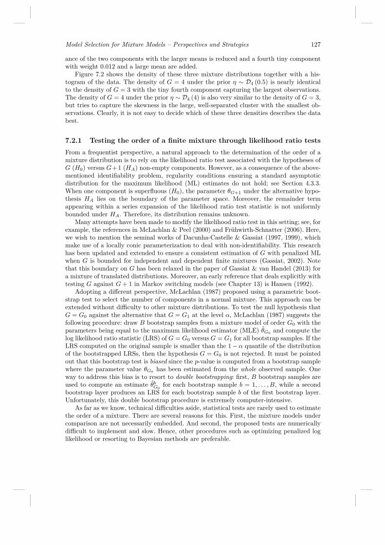
FIGURE 7.1Point process representation of the estimated mixture parameters for three mixture distri-butions fitted to the enzyme data using a Bayesian framework under the prior of Richardson& Green (1997). The size of each point (µg, σ2
g) corresponds to the mixture weight ηg. Top:G = 3. Bottom: G = 4 with η ∼ D4 (4) (left) and η ∼ D4 (0.5) (right; the very small fourthcomponent is marked by a circle).
estimators of G jointly with the unknown model parameters. Section 7.4 reviews such one-sweep Bayesian methods for cross-model inference on G, ranging from well-known methodssuch as reversible jump Markov chain Monte Carlo (MCMC) to more recent ideas involv-ing sparse finite mixtures relying on overfitting in combination with a prior on the weightdistribution that forces sparsity.
7.2 Selecting G as a Density Estimation ProblemWhen the estimation of the data distribution is the main purpose of the mixture modelling,it is generally assumed that this distribution truly is a finite mixture distribution. Oneinference issue is then to find the true number of mixture components, G, that is, theorder of the mixture behind the observations. This assumption is supposed to producewell-grounded tests and model selection criteria.
The true order of a finite mixture model is the smallest value of G such that the compo-nents of the mixture in (7.1) are all distinct and the mixing proportions are all positive (thatis, θg 6= θg′ , g 6= g′ and ηg > 0). This definition attempts to deal with the ambiguity (or

126 Handbook of Mixture Analysis
FIGURE 7.2Histogram of the enzyme data together with three fitted mixture distributions: G = 3 (solidline); G = 4 and η ∼ D4 (4) (dotted line); G = 4 and η ∼ D4 (0.5) (dashed line). The dashedand solid lines are nearly identical.
non-identifiability) due to overfitting, discussed in Section 1.3 of Chapter 1 and Section 4.2.2of Chapter 4: a mixture with G components can equally be defined as a (non-identifiable)mixture with G + 1 components where the additional component either has a mixing pro-portion ηG+1 equal to zero or the parameter θG+1 is identical to the parameter θg of someother component g ∈ {1, . . . , G}. These identifiability issues impact both frequentist andBayesian methods for selecting G. Hence, the order G is a poorly defined quantity and inpractical mixture analysis it is often difficult to decide what order G describes the databest.
By way of illustration, a mixture of normal distributions N (µg, σ2g) with G = 3 compo-
nents is fitted within a Bayesian framework to the enzyme data studied in Richardson &Green (1997), using the same prior as Richardson & Green, in particular a uniform prioron the weight distribution η = (η1, . . . , ηG). In addition, mixtures with G = 4 compo-nents are fitted, but with different symmetric Dirichlet priors for η, namely η ∼ D4 (4)and η ∼ D4 (0.5). As discussed in Section 4.2.2 above, the first prior favours overlappingcomponents, whereas the second prior favours small components, should the mixture beoverfitting.
Full conditional Gibbs sampling is applied for posterior inference. All three mixturemodels are identified by k-means clustering in the point process representation of the pos-terior draws of (µg, σg). The estimated component parameters (µg, σ2
g , ηg) are visualizedthrough a point process representation in Figure 7.1. Obviously, the parameters for thefour-component mixture are quite different and emerge in quite different ways than the com-ponents of the three-component mixture. The component (µg, σ2
g , ηg) = (0.19, 0.007, 0.61)is split into the two components (µg, σ2
g) = (0.16, 0.003) and (µg′ , σ2g′) = (0.26, 0.008) with
weights 0.38+0.23 = 0.61 under the prior η ∼ D4 (4). Under the prior η ∼ D4 (0.5), the vari-
Model Selection for Mixture Models – Perspectives and Strategies 127
ance of the two components with the larger means is reduced and a fourth tiny componentwith weight 0.012 and a large mean are added.
Figure 7.2 shows the density of these three mixture distributions together with a his-togram of the data. The density of G = 4 under the prior η ∼ D4 (0.5) is nearly identicalto the density of G = 3 with the tiny fourth component capturing the largest observations.The density of G = 4 under the prior η ∼ D4 (4) is also very similar to the density of G = 3,but tries to capture the skewness in the large, well-separated cluster with the smallest ob-servations. Clearly, it is not easy to decide which of these three densities describes the databest.
7.2.1 Testing the order of a finite mixture through likelihood ratio testsFrom a frequentist perspective, a natural approach to the determination of the order of amixture distribution is to rely on the likelihood ratio test associated with the hypotheses ofG (H0) versus G+1 (HA) non-empty components. However, as a consequence of the above-mentioned identifiability problem, regularity conditions ensuring a standard asymptoticdistribution for the maximum likelihood (ML) estimates do not hold; see Section 4.3.3.When one component is superfluous (H0), the parameter θG+1 under the alternative hypo-thesis HA lies on the boundary of the parameter space. Moreover, the remainder termappearing within a series expansion of the likelihood ratio test statistic is not uniformlybounded under HA. Therefore, its distribution remains unknown.
Many attempts have been made to modify the likelihood ratio test in this setting; see, forexample, the references in McLachlan & Peel (2000) and Frühwirth-Schnatter (2006). Here,we wish to mention the seminal works of Dacunha-Castelle & Gassiat (1997, 1999), whichmake use of a locally conic parameterization to deal with non-identifiability. This researchhas been updated and extended to ensure a consistent estimation of G with penalized MLwhen G is bounded for independent and dependent finite mixtures (Gassiat, 2002). Notethat this boundary on G has been relaxed in the paper of Gassiat & van Handel (2013) fora mixture of translated distributions. Moreover, an early reference that deals explicitly withtesting G against G+ 1 in Markov switching models (see Chapter 13) is Hansen (1992).
Adopting a different perspective, McLachlan (1987) proposed using a parametric boot-strap test to select the number of components in a normal mixture. This approach can beextended without difficulty to other mixture distributions. To test the null hypothesis thatG = G0 against the alternative that G = G1 at the level α, McLachlan (1987) suggests thefollowing procedure: draw B bootstrap samples from a mixture model of order G0 with theparameters being equal to the maximum likelihood estimator (MLE) θG0 and compute thelog likelihood ratio statistic (LRS) of G = G0 versus G = G1 for all bootstrap samples. If theLRS computed on the original sample is smaller than the 1−α quantile of the distributionof the bootstrapped LRSs, then the hypothesis G = G0 is not rejected. It must be pointedout that this bootstrap test is biased since the p-value is computed from a bootstrap samplewhere the parameter value θG0 has been estimated from the whole observed sample. Oneway to address this bias is to resort to double bootstrapping: first, B bootstrap samples areused to compute an estimate θbG0
for each bootstrap sample b = 1, . . . , B, while a secondbootstrap layer produces an LRS for each bootstrap sample b of the first bootstrap layer.Unfortunately, this double bootstrap procedure is extremely computer-intensive.
As far as we know, technical difficulties aside, statistical tests are rarely used to estimatethe order of a mixture. There are several reasons for this. First, the mixture models undercomparison are not necessarily embedded. And second, the proposed tests are numericallydifficult to implement and slow. Hence, other procedures such as optimizing penalized loglikelihood or resorting to Bayesian methods are preferable.

128 Handbook of Mixture Analysis
7.2.2 Information criteria for order selectionVarious information criteria for selecting the order of a mixture distribution are discussedin this section, including the Akaike (AIC) and Bayesian (BIC) information criteria (Sec-tion 7.2.2.1), the slope heuristic (Section 7.2.2.2), the deviance information criterion (DIC)(Section 7.2.2.3) , and the minimum message length (Section 7.2.2.4) and we refer to theliterature for additional criteria such as the approximate weight of evidence (AWE) crite-rion (Banfield & Raftery, 1993). Information criteria are based on penalizing the log of thelikelihood function Lo(θ;G), also known as the observed-data likelihood,
Lo(θ;G) =n∏i=1
[G∑g=1
ηgfg(yi | θg)], (7.3)
of a mixture modelMG with G components. The penalty is proportional to the number offree parameters inMG, denoted by υG, and the various criteria differ in the choice of thecorresponding proportionality factor. The number υG increases linearly in G and quantifiesthe complexity of the model. For a multivariate mixture of Gaussian distributions withunconstrained covariance matrices generating observations of dimension r, for instance,υG = G(1 + r + r(r + 1)/2)− 1.
7.2.2.1 AIC and BIC
Let θG be the MLE corresponding to the observed-data likelihood Lo(θ;G), defined in (7.3).The AIC (Akaike, 1974) and BIC (Schwarz, 1978) are popular model selection criteria forsolving the bias–variance dilemma for choosing a parsimonious model. AIC(G) is defined as
AIC(G) = −2 log `o(θG;G) + 2υG, (7.4)
whereas BIC(G) is defined as
BIC(G) = −2 log `o(θG;G) + υG log(n). (7.5)
Both criteria are asymptotic criteria and assume that the sampling pdf is within the modelcollection. On the one hand, the AIC aims to minimize the Kullback–Leibler divergencebetween model MG and the sampling pdf. On the other hand, the BIC approximates themarginal likelihood of modelMG, defined in (7.2), by ignoring the impact of the prior.
In some settings and under proper regularity conditions, the BIC can be shown tobe consistent, meaning it eventually picks the true order of the mixture, while the AIC isexpected to have a good predictive behaviour and happens to be minimax optimal, that is, tominimize the maximum risk among all estimators, in some regular situations (Yang, 2005).However, in a mixture setting both penalized log likelihood criteria face the same difficultiesas the likelihood ratio test due to the identifiability problems mentioned in Section 7.2.1.
When regularity conditions hold, the BIC is derived by a Laplace approximation of themarginal likelihood of modelMG:
p(y|G) =∫RυG
exp(nL(θ))dθ = exp (nL(θ∗G)) 2πn
υG/2 ∣∣−L′′(θ∗G)∣∣−1/2 +O(n−1),
where L : RυG −→ R is a C2 function, here
L(θ) = 1n
[log p(y|θ,G) + log p(θ|G)],
with unique maximum θ∗G. Moreover, the posterior mode θ∗G is approximately equal to

Model Selection for Mixture Models – Perspectives and Strategies 129
the MLE θG, and the Hessian of L can be approximated with the inverse of the Fisherinformation I(θG)−1. Hence,
−2 log p(y|G) = BIC(G) +O(1).
However, as noted above, the BIC is not truly Bayesian in that it bypasses all terms (firstand foremost the prior distribution) that do not depend on n. Moreover, if the (data-dependent) prior pdf p(θ|G) is a normal distribution deduced from the MLE distributionN (θG, I(θG)−1), then
−2 log p(y|G) = BIC(G) +O(n−1/2).
For this very reason, the BIC is mostly exploited for selecting a model estimated throughthe ML methodology (and not in a Bayesian way).
Under proper regularity conditions, the BIC enjoys the following asymptotic properties.
(a) The BIC is consistent: if there exists G∗ such that the true distribution p0 generatingthe data is equal to p(·|G∗), then, for n large enough, BIC selects G∗.
(b) Even if such a G∗ does not exist, good behaviour of the BIC can be expected, if p0 isclose to p(·|G∗) for the value G∗ selected by the BIC.
Unfortunately, the regularity conditions that validate the above Laplace approximationrequire the model parameters to be identifiable. As seen above, this is not true in generalfor most mixture models. However, the BIC has been shown to be consistent when the pdfsof the mixture components are bounded (Keribin, 2002). This is, for example, the case fora Gaussian mixture model with equal covariance matrices. In practice, there is no reason tothink that the BIC is not consistent for selecting the number of mixture components whenthe mixture model is used to estimate a density (see, for instance, Roeder & Wasserman,1997; Fraley & Raftery, 2002).
For singular models for which the Fisher information matrix is not everywhere invertible,Drton & Plummer (2017) proposed the so-called sBIC criterion. This criterion makes useof the Watanabe (2009) marginal likelihood approximation of a singular model. It is thesolution of a fixed point equation approximating the weighted average of the log marginallikelihoods of the models in competition. The sBIC criterion is proven to be consistent. Itcoincides with the BIC criterion when the model is regular. But, while the usual BIC is infact not Bayesian, the sBIC is connected to the large-sample behaviour of the log marginallikelihood (Drton & Plummer, 2017).
However, the BIC does not lead to a prediction of the observations that is asymptoti-cally optimal; see Yang (2005) and Drton & Plummer (2017) for further discussion on thecomparative properties of the AIC and BIC. In contrast to the BIC criterion, the AIC isknown to suffer from a marked tendency to overestimate the true value of G (see, for in-stance, Celeux & Soromenho (1996) for illustrations). However, a modification of AIC, theso-called AIC3 criterion, proposed in Bozdogan (1987), which replaces the penalty 2υG with3υG, provides a good assessment of G when the latent class model is used to estimate thedensity of categorical data (Nadif & Govaert, 1998). Nevertheless, the theoretical reasonsfor this interesting behaviour of the AIC3 (in this particular context) remain for the mostpart mysterious.
Finally, when the BIC is used to select the number of a mixture components for realdata, it has a marked tendency to choose a large number of components or even to choosethe highest proposed number of components. The reason for this behaviour is once morerelated to the fact that the penalty of the BIC is independent of the data, apart from thesample size n. When the bias in the mixture model does not vanish when the number ofcomponents increases, the BIC always increases by adding new mixture components. In a

130 Handbook of Mixture Analysis
model-based clustering context, this under-penalization tendency is often counterbalancedby the entropy of the mixture, added to rgw BIC in the ICLbic criterion (see Section7.3.2.1), which could lead to a compromise between the fit of a mixture model and itsability to produce a sensible clustering of the data. But there are many situations wherethe entropy of the mixture is not enough for counterbalancing this tendency and, moreover,the ICLbic is not really relevant when the modelling purpose is not related to clustering.
7.2.2.2 The Slope Heuristics
The so-called slope heuristics (Birgé & Massart, 2001, 2007), are a data-driven method tocalibrate a penalized criterion that is known up to a multiplicative constant κ. It has beensuccessfully applied to many situations, and particularly to mixture models when using theobserved-data log likelihood; see Baudry et al. (2012). As shown by Baudry (2015), it canbe extended without difficulty to other contrasts including the conditional classificationlog likelihood, which will be defined in Section 7.3.2.1. Roughly speaking, as with the AICand BIC, the penalty function pen(G) is assumed to be proportional to the number of freeparameters υG (i.e. the model dimension), pen(G) ∝ κυG.
The penalty is calibrated using the data-driven slope estimation (DDSE) procedure,available in the R package capushe (Baudry et al., 2012). The method assumes a linearrelation between the observed-data log likelihood and the penalty. It is important to notethat this assumption must and may easily be verified in practice via a simple plot. Thenthe DDSE procedure directly estimates the slope of the expected linear relationship be-tween the contrast (here the observed-data log likelihood, but other contrasts such as theconditional classification likelihood are possible) and the model dimension υG which is afunction of the number G of components. The estimated slope κ defines a minimal penaltyκυG below which smaller penalties give rise to the selection of more complex models, whilehigher penalties should select models with reasonable complexity. Arguments are providedin Birgé & Massart (2007) and Baudry et al. (2012) that the optimal (oracle) penalty isapproximately twice the minimal penalty. Thus, by setting the penalty to be 2κυG, theslope heuristics criterion is defined as
SH(G) = − log `o(θG;G) + 2κυG,
when considering mixture models in a density estimation framework. For more details aboutthe rationale and the implementation of the slope heuristics, see Baudry et al. (2012).
The slope heuristics method relies on the assumption that the bias of the fitted mod-els decreases as their complexity increases and becomes almost constant for the mostcomplex model. In the mixture model framework, this requires the family of models tobe roughly nested. More discussion, technical developments and illustrations are given inBaudry (2015).
The ability of the slope heuristics method, which is not based on asymptotic arguments,to detect the stationarity of the model family bias (namely the fact that the bias becomesalmost constant) is of prime relevance. It leads this criterion to propose more parsimoniousmodels than the BIC or even the integrated complete-data likelihood criterion (to be dis-cussed in Section 7.3.2.1). Many illustrations of this practical behaviour can be exhibited invarious domains of application of mixture models; see, for instance, a clustering use of theslope heuristics to choose the number of components of a multivariate Poisson mixture withRNASeq transcriptome data (Rau et al., 2015) or in a model-based clustering approach forcomparing bike sharing systems (Bouveyron et al., 2015).

Model Selection for Mixture Models – Perspectives and Strategies 131
7.2.2.3 DIC
In recent years, the deviance information criterion introduced by Spiegelhalter et al. (2002)has become a popular criterion for Bayesian model selection because it is easily computedfrom posterior draws, using MCMC methods. Like other penalized log likelihood criteria,the DIC involves a trade-off between goodness of fit and model complexity, measured interms of the so-called effective number of parameters. However, the use of the DIC to choosethe order G of a mixture model is not without issues, as discussed by De Iorio & Robert(2002) and Celeux et al. (2006).
To apply the DIC in a mixture context, several decisions have to be made. As for anylatent variable model, a first difficulty arises in the choice of the appropriate likelihoodfunction. Should the DIC be based on the observed-data log likelihood log p(y|θ,G), thecomplete-data log likelihood log p(y, z|θ,G) or the conditional log likelihood log p(y|z, θ, G),where z = (z1, . . . , zn) are the latent allocations generating the data (see also Section 7.3.1)?Second, the calculation of the DIC requires an estimate θG of the unknown parameter θwhich may suffer from label switching, making the DIC (which is based on averaging overMCMC draws) unstable. Finally, if the definition of the DIC involves either the complete-data or conditional likelihood, the difficulty that z is unobserved must be dealt with, eitherby integrating against the posterior p(z|y, G) or by using a plug-in estimator of z in whichcase once again the label switching problem must be addressed to avoid instability.
In an attempt to calibrate these difficulties, Celeux et al. (2006) investigate in total eightdifferent DIC criteria. DIC2, for instance, focuses on the marginal distribution of the dataand considers the allocations z as nuisance parameters. Consequently, it is based on theobserved-data likelihood:
DIC2(G) = −4Eθ (log p(y|θ,G)|y) + 2 log p(y|θG, G),
where the posterior mode estimator θG (which is invariant to label switching) is obtainedfrom the observed-data posterior p(θ|y, G) and Eθ is the expectation with respect to theposterior p(θ|y, G).
Based on several simulation studies, Celeux et al. (2006) recommend using DIC4 which isbased on computing first DIC for the complete-data likelihood function and then integratingover z with respect to the posterior p(z|y, G). This yields
DIC4(G) = −4Eθ,z (log p(y, z|θ,G)|y) + 2Ez
(log p(y, z|θG(z))|y
),
where θG(z) is the complete-data posterior mode which must be computed for each drawfrom the posterior p(z|y, G). This is straightforward if the complete-data posterior p(θg|y, z)is available in closed form. If this is not the case, Celeux et al. (2006) instead use the posteriormode estimator θG of the observed-data posterior p(θ|y). This leads to an approximationof DIC4(G), called DIC4a(G), which is shown to be a criterion that penalizes DIC2(G) bythe expected entropy, defined in (7.16):
DIC4a(G) = DIC2(G) + 2Eθ (ENT(θ;G)|y) .
Both DIC2(G) and DIC4a(G) are easily estimated from (MCMC) draws from the posteriorp(θ|y, G) by substituting all expectations E•(·|y) by an average over the correspondingdraws. Note that label switching is not a problem here, because both log p(y|θ,G) andENT(θ;G) are invariant to the labelling of the groups.
However, in practical mixture modelling, the DIC turns out to be very unstable, asshown by Celeux et al. (2006) for the galaxy data (Roeder, 1990). A similar behaviourwas observed by Frühwirth-Schnatter & Pyne (2010) who fitted skew-normal mixtures to

132 Handbook of Mixture Analysis
Alzheimer disease data under various prior assumptions. While the marginal likelihoodselected G = 2 with high confidence for all priors, DIC4a(G) selected G = 1, regardless ofthe chosen prior, whereas the number of components selected by DIC2(G) ranged from 2to 4, depending on the prior.
7.2.2.4 The minimum message length
Assuming that the form of the mixture models is fixed (e.g. Gaussian mixture models withfree covariance matrices or Gaussian mixture models with a common covariance matrix),several authors have proposed dealing with the estimation of the mixture parameters and Gin a single algorithm with the minimum message length (MML) criterion (see, for instance,Rissanen, 2012; Wallace & Freeman, 1987). Considering the MML criterion in a Bayesianperspective and choosing Jeffreys’ non-informative prior p(θ) for the mixture parameter,Figueiredo & Jain (2002) propose minimizing the criterion
MML(θ;G) = − log p(y|θ,G)− log p(θ|G) + 12 log |I(θ)|+ υG
2 (1− log(12)),
where I(θ) is the expected Fisher information matrix which is approximated by thecomplete-data Fisher information matrix IC(θ).
As we know, for instance from Section 4.2.2 above, Jeffreys’ non-informative prior doesnot work for mixtures. Figueiredo & Jain (2002) circumvent this difficulty by only consider-ing the parameters of the components whose proportion is non-zero, namely the componentsg such that ηg > 0.
Assuming, for instance, that the mixture model considered arises from the general Gaus-sian mixture family with free covariance matrices, this approach leads to minimizing thecriterion
MML(θ;G) =− log p(y|θ,G) + G?
2 log n
12
+ dim(θg)2
∑g:ηg>0
{log(n · dim(θg)/12) +G?(dim(θg) + 1)}, (7.6)
with G? = card{g|ηg > 0}. In this Bayesian context, the approach of Figueiredo & Jain(2002) involves optimizing iteratively the criterion (7.6), starting from a large number ofcomponents Gmax, and cancelling the components g such that, at iteration s,
n∑i=1
τ(s)ig <
dim(θ(s)g )
2 , (7.7)
where τ (s)ig are the elements of the fuzzy classification matrix defined in (7.18). Thus, the
chosen number of components G? is the number of components remaining at the conver-gence of the iterative algorithm. This iterative algorithm could be the EM algorithm, butFigueiredo & Jain (2002) argue that with EM, for large G, it can happen that no compo-nent has enough initial support, as the criterion for cancellation defined in (7.7) is fulfilledfor all G components. Thus, they prefer to make use of the componentwise EM algorithmof Celeux et al. (2001), which updates the ηg and the θg sequentially: update η1 and θ1,recompute τi1 for i = 1, . . . , n, update η2 and θ2, recompute τi2 for i = 1, . . . , n, and so on.
Zeng & Cheung (2014) use exactly the same approach with the completed-data or theclassification likelihood instead of the observed-data likelihood. Thus, roughly speaking, theprocedure of Figueiredo & Jain (2002) is expected to provide a similar number of componentsto the BIC, while the procedure of Zeng & Cheung (2014) is expected to provide a similarnumber of clusters to the ICLbic presented in Section 7.3.2.1.

Model Selection for Mixture Models – Perspectives and Strategies 133
7.2.3 Bayesian model choice based on marginal likelihoodsFrom a Bayesian testing perspective, selecting the number of components can be interpretedas a model selection problem, given the probability of each model within a collection of allmodels corresponding to the different numbers of components (Berger, 1985). The standardBayesian tool for making this model choice is based on the marginal likelihood (also calledevidence) of the data p(y|G) for each modelMG, defined in (7.2), which naturally penalizesmodels with more components (and more parameters) (Berger & Jefferys, 1992).
While the BIC is often considered as one case of information criterion, it is importantto recall (see Section 7.2.2.1) that it was first introduced by Schwartz (1965) as an approx-imation to the marginal likelihood p(y|G). Since this approximation does not depend onthe choice of the prior p(θ|G), it is not of direct appeal for a Bayesian evaluation of thenumber of components, especially when considering that the marginal likelihood itself canbe approximated by simulation-based methods, as discussed in this section.
7.2.3.1 Chib’s method, limitations and extensions
The reference estimator for evidence approximation is Chib’s (1995) representation of themarginal likelihood of modelMG as1
p(y|G) = p(y|θo, G)p(θo|G)p(θo|y, G) , (7.8)
which holds for any choice of the plug-in value θo. While the posterior p(θo|y, G) is notavailable in closed form for mixtures, a Gibbs sampling decomposition allows for a Rao–Blackwellized approximation of this density (Robert & Casella, 2004) that furthermoreconverges at a parametric speed, as already noticed in Gelfand & Smith (1990):
p(θo|y, G) = 1M
M∑m=1
p(θo|y, z(m), G),
where z(m),m = 1, . . . ,M , are the posterior draws for the latent allocations z = (z1, . . . , zn),introduced earlier in Chapter 1; see Chapter 5 for a review of posterior sampling methods.
However, for mixtures, the convergence of this estimate is very much hindered by the factthat it requires perfect symmetry in the Gibbs sampler, that is, complete label switchingwithin the simulated Markov chain. When the completed chain (z(m)
1 , . . . , z(m)n ) remains
instead concentrated around one single or a subset of the modes of the posterior distribution,the approximation of log p(θo|y, G) based on Chib’s representation fails, in that it is usuallyoff by a numerical factor of order O(log G!). Furthermore, this order cannot be used as areliable correction, as noted by Neal (1999) and Frühwirth-Schnatter (2006).
A straightforward method of handling Markov chains that are not perfectly mix-ing (which is the usual setting) is found in Berkhof et al. (2003) (see also Frühwirth-Schnatter, 2006, Section 5.5.5; Lee et al., 2009) and can be interpreted as a form of Rao–Blackwellization. The proposed correction is to estimate p(θo|y, G) as an average computedover all possible permutations of the labels, thus forcing the label switching and the ex-changeability of the labels to occur in a “perfect” manner. The new approximation can beexpressed as
p(θo|y, G) = 1MG!
∑s∈S(G)
M∑m=1
p(θo|y, s(z(m)), G) ,
1This was earlier called the candidate’s formula by Julian Besag (1989).

134 Handbook of Mixture Analysis
where S(G) traditionally denotes the set of the G! permutations of {1, . . . , G} and where sis one of those permutations. Note that the above correction can also be rewritten as
p(θo|y, G) = 1MG!
∑s∈S(G)
M∑m=1
p(s(θo)|y, z(m), G) , (7.9)
as this may induce some computational savings. Further savings can be found in the import-ance sampling approach of Lee & Robert (2016), who reduce the number of permutationsto be considered.
While Chib’s representation has often been advocated as a reference method for comput-ing the evidence, other methods abound within the literature, among them nested sampling(Skilling, 2007; Chopin & Robert, 2010), reversible jump MCMC (Green, 1995; Richardson& Green, 1997), particle filtering (Chopin, 2002), bridge sampling (Frühwirth-Schnatter,2004) and path sampling (Gelman & Meng, 1998). Some of these methods are discussednext.
7.2.3.2 Sampling-based approximations
If G is moderate, sampling-based techniques are particularly useful for estimating themarginal likelihood of finite mixture models; see Frühwirth-Schnatter (2004) and Lee &Robert (2016). Frühwirth-Schnatter (2004) considered three such estimation techniques,namely importance sampling, reciprocal importance sampling, and bridge sampling.
For sampling-based techniques, one selects an importance density qG(θ) which is easy tosample from and provides a rough approximation to the posterior density p(θ|y, G). Given asuitable importance density qG(θ), an importance sampling approximation to the marginallikelihood is based on rewriting (7.2) as
p(y|G) =∫p(y|θ,G)p(θ|G)
qG(θ) qG(θ)dθ.
Based on a sample θ(l) ∼ qG(θ), l = 1, . . . , L, from the importance density qG(θ), theimportance sampling estimator of the marginal likelihood is given by
pIS(y|G) = 1L
L∑l=1
p(y|θ(l), G)p(θ(l)|G)qG(θ(l))
. (7.10)
Gelfand & Dey (1994) introduced reciprocal importance sampling, which is based on theobservation that (7.8) can be written as
1p(y|G) = p(θ|y, G)
p(y|θ,G)p(θ|G) .
Integrating both sides of this equation with respect to the importance density qG(θ) yields
1p(y|G) =
∫qG(θ)
p(y|θ,G)p(θ|G)p(θ|y, G).
This leads to the reciprocal importance sampling estimator of the marginal likelihood,where the inverse of the ratio appearing in (7.10) is evaluated at the MCMC draws θ(m),m = 1, . . . ,M , and no draws from the importance density qG(θ) are required:
pRI(y|G) =(
1M
M∑m=1
qG(θ(m))p(y|θ(m), G)p(θ(m)|G)
)−1
.
Model Selection for Mixture Models – Perspectives and Strategies 135
These two estimators are special cases of bridge sampling (Meng & Wong, 1996):
p(y|G) =EqG(θ)(α(θ)p(y|θ,G)p(θ|G))
Ep(θ|y,G)(α(θ)qG(θ)) ,
with specific functions α(θ). The (formally) optimal choice for α(θ) yields the bridgesampling estimator pBS(y|G) and combines draws θ(l), l = 1, . . . , L, from the impor-tance density with MCMC draws θ(m), m = 1, . . . ,M . Using pIS(y|G) as a startingvalue for pBS,0(y|G), the following recursion is applied until convergence to estimatepBS(y|G) = limt→∞ pBS,t(y|G):
pBS,t(y|G) =L−1
L∑l=1
p(y|θ(l), G)p(θ(l)|G)LqG(θ(l)) +Mp(y|θ(l), G)p(θ(l)|G)/pBS,t−1(y|G)
M−1M∑m=1
qG(θ(m))LqG(θ(m)) +Mp(y|θ(m), G)p(θ(m)|G)/pBS,t−1(y|G)
. (7.11)
The reliability of these estimators depends on several factors. First, as shown by Frühwirth-Schnatter (2004), the tail behaviour of qG(θ) compared to the mixture posterior p(θ|y, G)is relevant. Whereas the bridge sampling estimator pBS(y|G) is fairly robust to the tail be-haviour of qG(θ), pIS(y|G) is sensitive if qG(θ) has lighter tails than p(θ|y, G), and pRI(y|G)is sensitive if qG(θ) has fatter tails than p(θ|y, G). Second, as pointed out by Lee & Robert(2016), for any of these methods it is essential that the importance density qG(θ) exhibits thesame kind of multimodality as the mixture posterior p(θ|y, G) and all modes of the posteriordensity are covered by the importance density also for increasing values of G. Otherwise,sampling-based estimators of the marginal likelihood are prone to be biased for the samereason Chib’s estimator is biased, as discussed in Section 7.2.3.1. A particularly stable esti-mator is obtained when bridge sampling is combined with a perfectly symmetric importancedensity qG(θ). Before the various estimators are illustrated for three well-known data sets(Richardson & Green, 1997), we turn to the choice of appropriate importance densities.
Importance densities for mixture analysis
As manual tuning of the importance density qG(θ) for each model under considerationis rather tedious, methods for choosing sensible importance densities in an unsupervisedmanner are needed. DiCiccio et al. (1997), for instance, suggested various methods to con-struct Gaussian importance densities from the MCMC output. However, the multimodal-ity of the mixture posterior density with G! equivalent modes evidently rules out such asimple choice. Frühwirth-Schnatter (1995) is one of the earliest references that used Rao–Blackwellization to construct an unsupervised importance density from the MCMC outputto compute marginal likelihoods via sampling-based approaches and applied this idea tomodel selection for linear Gaussian state space models. Frühwirth-Schnatter (2004) extendsthis idea to finite mixture and Markov switching models where the complete-data poste-rior p(θ|y, z) is available in closed form. Lee & Robert (2016) discuss importance samplingschemes based on (nearly) perfectly symmetric importance densities.
For a mixture distribution, where the component-specific parameters θg can be sampledin one block from the complete-data posterior p(θg|z,y), Rao–Blackwellization yields theimportance density
qG(θ) = 1S
S∑s=1
p(η|z(s))G∏g=1
p(θg|z(s),y), (7.12)

136 Handbook of Mixture Analysis
where z(s) are the posterior draws for the latent allocations. The construction of this import-ance density is fully automatic and it is sufficient to store the moments of these conditionaldensities (rather than the allocations z themselves) during MCMC sampling for later eval-uation. This method can be extended to cases where sampling θg from p(θg|z,y) requirestwo (or even more) blocks such as for Gaussian mixtures where θg = (µg, σ2
g) is sampled intwo steps from p(µg|σ2
g , z,y) and p(σ2g |µg, z,y).
Concerning the number of components in (7.12), on the one hand S should be small forcomputational reasons, because qG(θ) has to be evaluated for each of the S componentsnumerous times (e.g. L times for the importance sampling estimator (7.10)). On the otherhand, as mentioned above, it is essential that qG(θ) covers all symmetric modes of themixture posterior, and this will require a dramatically increasing number of components Sas G increases. Hence, any of these estimators is limited to moderate values of G, say up toG = 6.
Various strategies are available to ensure multimodality in the construction of the im-portance density. Frühwirth-Schnatter (2004) chooses S = M and relies on random per-mutation Gibbs sampling (Frühwirth-Schnatter, 2001) by applying a randomly selectedpermutation sm ∈ S(G) at the end of the mth MCMC sweep to define a permutationz(s) = sm(z(m)) of the posterior draw z(m) of the allocation vector. The random permuta-tions s1, . . . , sM guarantee multimodality of qG(θ) in (7.12); however, as discussed above,it is important to ensure good mixing of the underlying permutation sampler over all G!equivalent posterior modes. Only if S is large compared to G! are all symmetric modesvisited by random permutation sampling. Choosing, for instance, S = S0G! ensures thateach mode is visited on average S0 times.
As an alternative to random permutation sampling, approaches exploiting full permuta-tions have been suggested; see, for example, Frühwirth-Schnatter (2004). Importance sam-pling schemes exploiting full permutation were discussed in full detail in Lee & Robert(2016). The definition of a fully symmetric importance density qG(θ) is related to the cor-rection for Chib’s estimator discussed earlier in (7.9):
qG(θ) = 1S0G!
∑s∈S(G)
S0∑s=1
p(η|s(z(s)))G∏g=1
p(θg|s(z(s)),y). (7.13)
This construction, which has S = S0G! components, is based on a small number S0 ofparticles z(s), as qG(θ) needs to be only a rough approximation to the mixture posteriorp(θ|y, G) and estimators such as bridge sampling will be robust to the tail behaviour ofqG(θ). In (7.13), all symmetric modes are visited exactly S0 times. The moments of theS0 conditional densities need to be stored for only one of the G! permutations and, again,this construction can be extended to the case where the components of θg are sampled inmore than one block. Lee & Robert (2016) discuss strategies for reducing the computationalburden associated with evaluating qG(θ).
Frühwirth-Schnatter (2006, p. 146) and Lee & Robert (2016) discuss a simplified versionof (7.13) where the random sequence z(s), s = 1, . . . , S0, is substituted by a single optimalpartition z? such as the maximum a posteriori (MAP) estimator:
qG(θ) = 1G!
∑s∈S(G)
p(θ|s(z?),y).
In MATLAB, the bayesf package (Frühwirth-Schnatter, 2018) allows one to estimatepBS(y|G), pIS(y|G) and pRI(y|G) with the importance density being constructed eitheras in (7.12) using random permutation sampling or as in (7.13) using full permutationsampling.
Model Selection for Mixture Models – Perspectives and Strategies 137
Example: Marginal likelihoods for the data sets in Richardson & Green (1997)
By way of illustration, marginal likelihoods are computed for mixtures of G univariatenormal distributions N (µg, σ2
g) for G = 2, . . . , 6 for the acidity data, the enzyme data andthe galaxy data studied by Richardson & Green (1997) in the framework of reversible jumpMCMC (see Section 7.4.2 for a short description of this one-sweep method). We use thesame priors as Richardson & Green, namely the symmetric Dirichlet prior η ∼ DG (1), thenormal prior µg ∼ N (m,R2), the inverse gamma prior σ2
g ∼ IG(2, C0) and the gamma priorC0 ∼ G(0.2, 10/R2), where m and R are the midpoint and the length of the observationinterval. For a given G, full conditional Gibbs sampling is performed for M = 12,000draws after a burn-in of 2000, by iteratively sampling from p(σ2
g |µg, C0, z,y), p(µg|σ2g , z,y),
p(C0|σ21 , . . . , σ
2G), p(η|z) and p(z|θ,y).
A fully symmetric importance density qG,F (θ) is constructed from (7.13), where S0 = 100components are selected for each mode. For comparison, an importance density qG,R(θ) isconstructed from (7.12) with S = S0G!, ensuring that for random permutation samplingeach mode is visited on average S0 times. However, unlike qG,F (θ), the importance densityqG,R(θ) is not fully symmetric. Ignoring the dependence between µg and σ2
g , the componentdensities are constructed from conditionally independent densities, given the sth draw of(z, θ1, . . . , θG, C0):
p(µg, σ2g |z(s), θ(s)
g , C(s)0 ,y) = p(µg|σ2,(s)
g , z(s),y)p(σ2g |µ(s)
g , C(s)0 , z(s),y).
Prior evaluation is based on the marginal prior p(σ21 , . . . , σ
2G), where C0 is integrated out.
This yields in total six estimators, pBS,F (y|G), pIS,F (y|G) and pRI,F (y|G) for full per-mutation sampling and pBS,R(y|G), pIS,R(y|G) and pRI,R(y|G) for random permutationsampling, for each G = 2, . . . , 6. For each estimator, standard errors SE are computed asin Frühwirth-Schnatter (2004). Results are visualized in Figure 7.3, by plotting all six esti-mators p•(y|G) as well as p•(y|G) ± 3 SE over G for all three data sets. Good estimatorsshould be unbiased with small standard errors and the order in which the six estimatorsare arranged (which is the same for all Gs) is related to this quality measure.
There is a striking difference in the reliability of the six estimators, in particular asG increases. Reciprocal importance sampling is particularly unreliable and the estimatedvalues of log pRI,R(y|G) under qG,R(θ) tend to be extremely biased for G ≥ 4, even if thebias is reduced to a certain extent by choosing the fully symmetric importance densityqG,F (θ). Also the two other estimators log pIS,R(y|G) and log pBS,R(y|G) tend to be biasedunder qG,R(θ), and bridge sampling is more sensitive than importance sampling to choosingan importance density that is not fully symmetric.
Unlike for reciprocal importance sampling, the bias disappears for both bridge sam-pling and importance sampling under the fully symmetric importance density qG,F (θ), andlog pIS,F (y|G) and log pBS,F (y|G) yield more or less identical results. However, due to therobustness of bridge sampling with respect to the tail behaviour of qG,F (θ), we find that thestandard errors of log pBS,F (y|G) are often considerably smaller than the standard errorsof log pIS,F (y|G), in particular for the enzyme data.
Based on log pBS,F (y|G), marginal likelihood evaluation yields the following results forthe three data sets. For the acidity data, log pBS,F (y|G = 3) = −198.2 and log pBS,F (y|G =4) = −198.3 are more less the same, with the log odds of G = 3 over G = 4 being equalto 0.1. Also for the enzyme data, with log pBS,F (y|G = 3) = −74.2 and log pBS,F (y|G =4) = −74.3, the log odds of G = 3 over G = 4 are equal to 0.1. Finally, for the galaxydata, log pBS,F (y|G = 5) = log pBS,F (y|G = 6) = −225.9. Hence, under the prior p(θ|G)employed by Richardson & Green (1997), for all three data sets no clear distinction can bemade between two values of G based on the marginal likelihood. However, if the marginallikelihoods are combined with a prior on the number of components such as G− 1 ∼ P(1)

138 Handbook of Mixture Analysis
FIGURE 7.3Marginal likelihood estimation for the benchmarks in Richardson & Green (1997): the acid-ity data (top), the enzyme data (middle) and the galaxy data (bottom) over G = 2, . . . , G =6. For each G, six estimators p•(y|G) are given together with p•(y|G) ± 3SE in the orderpBS,F (y|G), pIS,F (y|G), pIS,R(y|G), pBS,R(y|G), pRI,F (y|G) and pRI,R(y|G) from left toright.

Model Selection for Mixture Models – Perspectives and Strategies 139
(Nobile, 2004), then the log posterior odds, being equal to 1.5 for the acidity and the enzymedata and 1.8 for the galaxy data, yield evidence for the smaller of the two values of G forall three data sets.
7.3 Selecting G in the Framework of Model-Based ClusteringAssuming that the data stem from one of the models under comparison is most oftenunrealistic and can be misleading when using the AIC or BIC. Now a common feature ofstandard penalized likelihood criteria is that they abstain from taking the modelling purposeinto account, except when inference is about estimating the data density. In particular,misspecification can lead to overestimating the complexity of a model in practical situations.Taking the modelling purpose into account when selecting a model leads to alternative modelselection criteria that favor useful and parsimonious models. This viewpoint is particularlyrelevant when considering a mixture model for model-based clustering; see Chapter 8 for areview of this important application of mixture models.
7.3.1 Mixtures as partition modelsClustering arises in a natural way when an i.i.d. sample is drawn from the finite mixturedistribution (7.1) with weights η = (η1, . . . , ηG). As explained in Chapter 1, Section 1.1.3,each observation yi can be associated with the component, indexed by zi, that generatedthis data point:
zi|η ∼M(1, η1, . . . , ηG), (7.14)yi|zi ∼ fzi(yi|θzi).
Let z = (z1, . . . , zn) be the collection of all component indicators that were used to generatethe n data points y = (y1, . . . , yn). Obviously, z defines a partition of the data. A clusterCg = {i|zi = g} is thus defined as a subset of the data indices {1, . . . , n}, containing allobservations with identical allocation variables zi. Hence, the indicators z define a partitionC = {C1, . . . , CG+} of the n data points, where yi and yj belong to the same cluster if andonly if zi = zj . The partition C contains G+ = |C| clusters, where |C| is the cardinality ofC. In a Bayesian context, finite mixture models imply random partitions over the lattice
SnG = {(z1, . . . , zn) : zi ∈ {1, . . . , G}, i = 1, . . . , n},
as will be discussed in detail in Section 7.3.3.In model-based clustering, a finite mixture model is applied to recover the (latent)
allocation indicators z from the data and to estimate a suitable partition of the data. Auseful quantity in this respect is the so-called fuzzy classification matrix τ . The elementsτig, with i = 1, . . . , n and g = 1, . . . , G, of τ are equal to the conditional probability thatobservation yi arises from component g in a mixture model of order G given yi:
τig = P(zi = g|yi, θ) = P(zig = 1|yi, θ) = ηgfg(yi | θg)∑Gj=1 ηjfj(yi | θj)
, (7.15)
where zig = I(zi = g). The entropy ENT(θ;G) corresponding to a fuzzy classification matrixτ is defined as
ENT(θ;G) = −G∑g=1
n∑i=1
τig log τig ≥ 0. (7.16)

140 Handbook of Mixture Analysis
Both τ and ENT(θ;G) are data-driven measures of the ability of a G-component mixturemodel to provide a relevant partition of the data. If the mixture components are wellseparated for a given θ, then the classification matrix τ tends to define a clear partition ofthe data set y = (y1, . . . , yn), with τig being close to 1 for one component and close to 0for all other components. In this case, ENT(θ;G) is close to 0. On the other hand, if themixture components are poorly separated, then ENT(θ;G) takes values larger than zero.The maximum value ENT(θ;G) can take is n logG, which is the entropy of the uniformdistribution which assigns yi to all G clusters with the same probability τig ≡ 1/G.
In a Bayesian context, the fuzzy classification matrix is instrumental for joint estimationof the parameter θ and z within Gibbs sampling using data augmentation (see, for example,Robert & Casella, 2004). In a frequentist framework, the estimated classification matrix τ ,given a suitable estimate θG of the mixture parameters θ (e.g. the MLE), can be used toderive an estimator z of the partition of the data; see also Chapter 8, Section 8.2.4. As willbe discussed in Section 7.3.2, the entropy of the estimated classification matrix τ plays animportant role in defining information criteria for choosing G in a clustering context.
7.3.2 Classification-based information criteriaAs discussed in Section 7.2.2.1 within the framework of density estimation, the BIC en-joys several desirable properties; however, within cluster analysis it shows a tendency tooverestimate G; see, for instance, Celeux & Soromenho (1996). The BIC does not take theclustering purposes for assessing G into account, regardless of the separation of the clusters.To overcome this limitation, an attractive possibility is to select G so that the resultingmixture model leads to the clustering of the data with the largest evidence. This is the pur-pose of various classification-based information criteria such as the integrated complete-datalikelihood criterion that are discussed in this subsection.
In a classification context, it is useful to state a simple relation linking the log of theobserved-data density p(y|θ) and the complete-data density p(y, z|θ). The observed-datalog likelihood of θ for a sample y, denoted by log `o(θ;G), is given by
log `o(θ;G) =n∑i=1
log[G∑g=1
ηgfg(yi | θg)],
whereas the complete-data log likelihood of θ for the complete sample (y, z), denoted bylog `c(θ;G), reads
log `c(θ, z;G) =n∑i=1
G∑g=1
zig log(ηgfg(yi | θg)),
where zig = I(zi = g), g = 1, . . . , G. These log likelihoods are linked in the following way:
log `c(θ, z;G) = log `o(θ;G)− EC(θ, z;G), (7.17)
where
EC(θ, z;G) = −G∑g=1
n∑i=1
zig log τig ≥ 0.
Since E(zig|θ, yi) = P(zig = 1|θ, yi) = τig, we obtain that the expectation of EC(θ, z;G) withrespect to the conditional distribution p(z|y, θ) for a given θ is equal the entropy ENT(θ;G)defined in (7.16). Hence, the entropy can be regarded as a penalty for the observed-datalikelihood in cases where the resulting clusters are not well separated.

Model Selection for Mixture Models – Perspectives and Strategies 141
7.3.2.1 The integrated complete-data likelihood criterion
The integrated (complete-data) likelihood related to the complete data (y, z) is
p(y, z | G) =∫
ΘGp(y, z | G, θ)p(θ | G)dθ,
where
p(y, z | G, θ) =n∏i=1
p(yi, zi | G, θ) =n∏i=1
G∏g=1
ηzigg [fg(yi | θg)]zig .
This integrated complete-data likelihood (ICL) takes the missing data z into account andcan be expected to be relevant for choosing G in a clustering context. However, computingthe ICL is challenging for various reasons. First, computing the ICL involves an integrationin high dimensions. Second, the labels z are unobserved (missing) data. To approximatethe ICL, a BIC-like approximation is possible (Biernacki et al., 2000):
log p(y, z | G) ≈ log p(y, z | G, θz)− υG2 logn,
whereθz = arg max
θp(y, z | G, θ),
and υG is the number of free parameters of the mixture modelMG. Note that this approx-imation involves the complete-data likelihood, Lc(θ, z;G) = p(y, z | G, θ); however, z and,consequently, θz are unknown. First, approximating θz ≈ θG, with θG being the MLE of theG-component mixture parameter θ, is expected to be valid for well-separated components.Second, given θG, the missing data z are imputed using the MAP estimator z = MAP(θG)defined by
zig ={
1, if argmaxlτil(θG) = g,0, otherwise.
This leads to the criterion
ICLbic(G) = log p(y, z | G, θG)− υG2 logn.
Exploiting (7.17), one obtains that the ICLbic criterion takes the form of a BIC criterion,penalized by the estimated entropy
ENT(θG;G) = −G∑g=1
n∑i=1
τig log τig ≥ 0,
with τig denoting the conditional probability that yi arises from the gth mixture component(i = 1, . . . , n, g = 1, . . . , G) under the parameter θG; see (7.15).
Because of this additional entropy term, the ICLbic criterion favours values of G givingrise to partitions of the data with the highest evidence. In practice, the ICLbic appears toprovide a stable and reliable estimation of G for real data sets and also for simulated datasets from mixtures when the components do not overlap too much. However, it should benoted that the ICLbic, which is not concerned with discovering the true number of mixturecomponents, can underestimate the number of components for simulated data arising frommixtures with poorly separated components.

142 Handbook of Mixture Analysis
2 2.5 3 3.5 4 4.5 5
45
50
55
60
65
70
75
80
85
90
95
eruptions
waiting
2 2.5 3 3.5 4 4.5 5
45
50
55
60
65
70
75
80
85
90
95
eruptions
waiting
FIGURE 7.4Cluster ellipses for the Old Faithful Geyser data: (left) the BIC solution; (right) the ICLbicsolution.
An illustrative comparison of the BIC and ICLbic
Obviously, in many situations where the mixture components are well separated, the BICand ICLbic select the same number of mixture components. But the following small numer-ical example aims to illustrate a situation where these two criteria give different answers.
We start from a benchmark (genuine) data set known as the Old Faithful Geyser. Eachof the 272 observations consists of two measurements: the duration of the eruption and thewaiting time before the next eruption of the Old Faithful Geyser, in Yellowstone NationalPark, USA. We consider a bivariate Gaussian mixture model with component densitiesN (µk,Σk) with unconstrained covariance matrices Σk.
For this data set, Figure 7.4 shows that the ICLbic selects with a large evidence G = 2,while the BIC slightly prefers G = 3 to G = 2. The BIC solution with G = 3 componentsappears to model deviations from normality in one of the two obvious clusters, rather thana relevant additional cluster.
7.3.2.2 The conditional classification likelihood
In a model-based clustering context where a cluster is associated with a mixture component,it is sensible in view of (7.17) to maximize the conditional expectation of the complete-datalog likelihood (Baudry, 2015),
logLcc(θ;G) = Ez(log `c(θ, z;G)) = log `o(θ;G)− ENT(θ;G),
rather than the observed-data log likelihood function log `o(θ;G). This can be done throughan EM-type algorithm where the M step at iteration s+ 1 involves finding
θ(s+1) ∈ argmaxθ∈ΘG
(log `o(θ;G) +
n∑i=1
G∑g=1
τ(s)ig log τig
), (7.18)
where the τig are defined as in (7.15) and
τ(s)ig = η
(s)g fg(yi | θ(s)
g )∑Gj=1 η
(s)j fj(yi | θ(s)
j ).
This M step can be performed by using an adaptation of the so-called Bayesian expectationmaximization (BEM) of Lange (1999). The resulting algorithm inherits the fundamental
Model Selection for Mixture Models – Perspectives and Strategies 143
property of EM to increase the criterion logLcc(θ), which does not depend on z, at eachiteration.
In this context, Baudry (2015) considered choosing G from a penalized criterion of theform
Lcc-ICL(G) = − logLcc(θMLccEG ;G) + pen(G),
where θMLccEG = arg maxθ logLcc(θ;G). Under regularity conditions and the standard condi-
tion for information criteria the following holds. Assuming that pen : {1, . . . , Gmax} → R+
satisfies {pen(G) = oP(n), as n→∞,(pen(G)− pen(G′)
) P−−−−→n→∞
∞, if G′ < G,
and defining G = min argminG Lcc-ICL(G), Baudry (2015) proved that
P[G 6= G0
]−−−−→n→∞
0,
where G0 is the minimum number of components such that the bias of the models is sta-tionary for G ≥ G0,
G0 = min argmaxG
Ep0
[log `c(θ0
G)],
withθ0G = argmin
θ∈ΘG
{dKL
(p0, p( . ; θ)
)+ Ep0
[EC(θ;G)
]},
dKL(p0, p( . ; θ)
)being the Kullback–Leibler distance between the true distribution p0 of
the data and the mixture distribution with parameter θ. Moreover, Baudry (2015) deducesthat, by analogy with the BIC, an interesting identification criterion to be minimized is
Lcc-ICL(G) = − logLcc(θMLccEG ;G) + υG
2 logn.
The criterion ICLbic can thus be viewed as an approximation of Lcc-ICL. Therefore, thecriterion Lcc-ICL underlies a notion of class that is a compromise between the “mixturecomponent” and the “cluster” points of view.
7.3.2.3 Exact derivation of the ICL
Like the BIC, the ICL has been defined in a Bayesian framework, but its asymptotic ap-proximations ICLbic and Lcc-ICL are not intrinsically Bayesian, since they do not dependon the associated prior distribution. However, if the mixture components belong to theexponential family, it is possible to get closed-form expressions for the ICL (see Biernackiet al., 2010, or Bertoletti et al., 2015). With such closed-form expressions, it is possible tocompute the ICL values by replacing the missing labels z with their most probable valuesusing the MAP operator after estimating the parameter θG as the posterior mode or theMLE (see Biernacki et al., 2010). An alternative is to optimize the exact ICL in z. Thelimitations of approaches based on exact ICL computing are twofold.
Choosing non-informative prior distributions
Except for categorical data which involve mixtures of multivariate discrete distributions,there is no proper consensual non-informative prior distribution for other classes of mix-ture models such as Gaussian or Poisson mixture models (see Chapter 4). It is obviouslypossible to choose exchangeable weakly informative hyperparameters with conjugate priordistributions for the parameters of the mixture components. However, the posterior distri-bution and thus the resulting ICL values will inevitably depend on these hyperparameters.

144 Handbook of Mixture Analysis
For the latent class model on categorical data, deriving the exact ICL is easier, since thenon-informative conjugate Dirichlet prior distributions DG (e0) are proper for the weightdistribution of the mixture. Following the recommendation of Frühwirth-Schnatter (2011),it has been demonstrated that choosing e0 = 4 is expected to provide a stable selectionof G (see, for instance, Keribin et al., 2015). Numerical experiments on simulated dataproved that exact ICL computed with plug-in estimates θG of the parameter could providedifferent and more reliable estimation of G than the ICLbic for small sample sizes. Thus,when conjugate non-informative prior distributions are available, deriving a non-asymptoticapproximation of ICL can be feasible.
Optimizing the exact ICL
Several authors have considered the direct optimization of the exact ICL in z withoutestimating θ. Bertoletti et al. (2015), Côme & Latouche (2015) and Wyse et al. (2017)have proposed greedy algorithms, while Tessier et al. (2006) proposed using evolutionaryoptimization algorithms. At this point, it is important to remark that the optimizationproblem has to be solved in a search space with about O(Gnmax) elements, where Gmax isthe maximum number of components allowed. This means that the optimization problembecomes quite formidable for n large. In addition, the proposed greedy algorithms are highlysensitive to the numerous local optima and have only been experimented with for moderatesample sizes. This is the reason why evolutionary algorithms are expected to be useful butthey need to be calibrated (to choose the tuning parameters) and are expensive in computingtime.
7.3.3 Bayesian clusteringIn the context of Bayesian clustering (see Lau & Green, 2007, for an excellent review),where the allocation indicator z = (z1, . . . , zn) is regarded as a latent variable, a finitemixture model implies random partitions over the lattice SnG. Hence, for a given order Gof the mixture distribution (7.1), both the prior density p(z|G) and the posterior densityp(z|G,y) are discrete distributions over the lattice SnG. Although this induces a change ofprior modelling, Lau & Green (2007) discuss Bayesian nonparametric (BNP; see Chapter6) methods to estimate the number of clusters. We discuss the BNP perspective further inSection 7.4.4 and refer to Chapter 6 for a comprehensive treatment.
For a finite mixture model, the Dirichlet prior η ∼ D(e1, . . . , eG) on the weight dis-tribution strongly determines what the prior distribution p(z|G) looks like. To preservesymmetry with respect to relabelling, typically the symmetric Dirichlet prior DG (e0) isemployed, where e1 = . . . = eG = e0. The corresponding prior p(z|G) =
∫ ∏ni=1 p(zi|η)d η
is given by
p(z|G) = Γ(Ge0)Γ(n+Ge0)Γ(e0)G+
∏g:ng>0
Γ(ng + e0), (7.19)
where ng =∑ni=1 I(zi = g) is the number of observations in cluster g and G+ is defined as
the number of non-empty clusters,
G+ = G−G∑g=1
I(ng = 0). (7.20)
As mentioned earlier, in model-based clustering interest lies in estimating the number ofclusters G+ in the n data points rather than the number of components G of the mixture
Model Selection for Mixture Models – Perspectives and Strategies 145
distribution (7.1), and it is important to distinguish between both quantities. Only a fewpapers make this clear distinction between the number of mixture components G and thenumber of data cluster G+ for finite mixture models (Nobile, 2004; Miller & Harrison, 2018;Malsiner-Walli et al., 2017; Frühwirth-Schnatter & Malsiner-Walli, 2018).
A common criticism concerning the application of finite mixture models in a clusteringcontext is that the number of components G needs to be known a priori. However, what isyet not commonly understood is (a) that the really relevant question is whether or not thenumber of clusters G+ in the data is known a priori and (b) that even a finite mixture with afixed value of G can imply a random prior distribution on G+. By way of further illustration,let ng =
∑ni=1 I(zi = g) be the number of observations generated by the components
g = 1, . . . , G. Then (7.14) implies that n1, . . . , nG follow a multinomial distribution:
n1, . . . , nG|η ∼M(n, η1, . . . , ηG). (7.21)
Depending on the weights η = (η1, . . . , ηG) appearing in the mixture distribution (7.1),multinomial sampling according to (7.21) may lead to partitions with ng being zero, leadingto so-called “empty components”. In this case, fewer than G mixture components were usedto generate the n data points which contain G+ non-empty clusters, where G+ is definedas in (7.20).
In a Bayesian framework towards finite mixture modelling, the Dirichlet prior η ∼DG (e0) on the component weights controls whether, a priori, G+ is equal to G and noempty components occur. In particular, if e0 is close to 0, then G+ is a random variabletaking a priori values smaller than G with high probability. Exploiting the difference be-tween G+ and G in an overfitting mixture with a prior on the weight distribution thatstrongly shrinks redundant component weights towards 0 is a cornerstone of the concept ofsparse finite mixtures (Malsiner-Walli et al., 2016) which will be discussed in Section 7.4.5as a one-sweep method to determine G+ for a fixed G.
In Bayesian clustering (rather than Bayesian mixture estimation), the main object ofinterest is the (marginal) posterior of the allocations z, rather than the (marginal) posteriordistribution of the mixture parameters θ. Depending on the mixture under investigation, theintegrated likelihood p(y|z, G) for G known may be available in closed form, in particular,if the component densities fg(y|θg) come from exponential families and a conditionallyconjugate prior p(θg) is employed for θg. As noted, for instance, by Casella et al. (2004), formany mixture models it is then possible to derive an explicit form for the marginal posteriorp(z|y, G) of the indicators z, where dependence on the parameter θ is integrated out. ByBayes’ theorem, the marginal posterior p(z|y, G) is given by
p(z|y, G) ∝ p(y|z, G)p(z|G), (7.22)
where the integrated prior p(z|G) is given by (7.19) and the integrated likelihood p(y|z, G)takes the form
p(y|z, G) =∫p(y|z, θ1, . . . , θG, η,G)p(θ1, . . . , θG, η|G)d(θ1, . . . , θG, η). (7.23)
To explore the posterior of the allocations, efficient methods to sample from the posteriorp(z|y, G) are needed, and some of these methods will be discussed in Section 7.4.3. Thisexploration is quite a computational challenge, as the size of the lattice SnG increases rapidlywith both the number n of observations and the number G of components and is given bythe Bell number. For n = 10 and G = 3, for instance, there are 59,049 different allocationsz, whereas for n = 100 and G = 3 the number of different allocations is of the order of5 · 1047. This means that it is impossible to visit all possible partitions C during posteriorsampling and many partitions are visited at best once.

146 Handbook of Mixture Analysis
FIGURE 7.5Bayesian clustering of the galaxy data (Roeder, 1990), assuming a Gaussian mixture withG = 5 components. The data are indicated through a rug plot. Partitions resulting fromthe MAP estimator (top), the minimum risk estimator (middle) and minimizing Binder’sloss function.
This large set of partitions raises the question of how to summarize the posteriorp(z|y, G), given posterior simulations. Common summaries are based on deriving pointestimators z, such as the MAP estimator, the minimum risk estimator or the partitionminimizing Binder’s loss function (Binder, 1978), see Section 8.3.2 for more details. How-ever, these estimators (even if they differ) do not fully reflect the uncertainty in assigningobservations to clusters.
By way of illustration, a mixture of univariate Gaussian distributions is used for Bayesianclustering of the galaxy data (Roeder, 1990), assuming that G = 5 is fixed. Prior specifi-cation follows Richardson & Green (1997), and 12,000 draws from p(z|y, G) are obtainedusing full conditional Gibbs sampling. In Figure 7.5, various point estimators z derivedfrom the posterior draws of z are displayed, together with a rug plot of the data. While theMAP estimator and the estimator minimizing Binder’s loss function are invariant to labelswitching, the minimum risk estimator is based on an identified model. Label switching isresolved by applying k-means clustering to the point process representation of the MCMCdraws of (µg, σg). Classification over the various point estimators z is stable for observationsin the two clusters capturing the tails, but the classification for observations in the centreof the distribution tends to be rather different.
To quantify such uncertainty, Wade & Gharhamani (2018) develop not only appropri-ate point estimates, but also credible sets to summarize the posterior distribution of thepartitions based on decision- and information-theoretic techniques.

Model Selection for Mixture Models – Perspectives and Strategies 147
7.3.4 Selecting G under model misspecificationMixture models are a very popular tool for model-based clustering, in both the frequentistand Bayesian frameworks. However, success in identifying meaningful clusters in the datavery much hinges on specifying sensible component densities, and Bayesian inferences to-wards estimating the number of clusters are sensitive to misspecifications of the componentdensities, as are most penalized likelihood criteria discussed in the previous subsections.Most commonly, a finite mixture model with (multivariate) Gaussian component densitiesis fitted to the data to identify homogeneous data clusters within a heterogeneous popula-tion:
y ∼G∑g=1
ηgN (µg,Σg). (7.24)
Similarly to the likelihood approach, Bayesian cluster analysis has to address several issues.First, as discussed above, even if we fit a correctly specified mixture model (7.1) to datagenerated by this model, an estimate of the number of components G will not necessarilybe a good estimator of the number of clusters G+ in the data, and a more reliable estimateis obtained when exploring the partitions.
However, problems with the interpretation of G+ might nevertheless occur, in particularif the component density is misspecified and several components have to be merged toaddress this misspecification. A typical example is fitting the multivariate Gaussian mixturedistribution (7.24) to data such as the Old Faithful Geyser data. As shown in Figure 7.4,more than one Gaussian component is needed to capture departure from normality such asskewness and excess kurtosis for one of the two clusters. As discussed before, the BIC isparticularly sensitive to this kind of misspecification, and classification-based informationcriteria such as the ICL criterion introduced in Section 7.3.2.1 are more robust in thisrespect.
In both Bayesian and frequentist frameworks, misspecification has been resolved bychoosing more flexible distributions for the components densities. Many papers demonstratethe usefulness of mixtures of parametric non-Gaussian component densities in this context(see Frühwirth-Schnatter & Pyne, 2010, and Lee & McLachlan, 2013, among many others),and Chapter 10 also addresses this problem. Unsurprisingly, the estimated G+ of such anon-Gaussian mixture often provides a much better estimator of the number of clusters thandoes the Gaussian mixture. With respect to inference, the Bayesian framework offers a slightadvantage, as MCMC methods are able to deal with non-standard component densities ina more flexible way than the EM algorithm.
In higher dimensions it might be difficult to choose an appropriate parametric distribu-tion for characterizing a data cluster, and mixture models with more flexible (not necessarilyparametric) cluster densities turn out to be useful. The mixture of Gaussian mixtures ap-proach, for instance, exploits the ability of normal mixtures to accurately approximate awide class of probability distributions, and models the non-Gaussian cluster distributionsthemselves by Gaussian mixtures. This introduces a hierarchical framework where in theupper level a non-Gaussian mixture is fitted as in (7.1), whereas at a lower level eachcomponent density fg(y|θg) itself is described by a mixture of Hg Gaussian distributions.On the upper level, G+ is identified as the number of such clusters, whereas the numberof subcomponents Hg in each cluster reflects the quality of the semi-parametric mixtureapproximation.
Two different approaches are available to “estimate” the number of clusters in sucha framework. Any such approach has to deal with the following additional identifiabilityproblems for this type of mixtures: the observed-data likelihood ascertains this model justas one big mixture of Gaussian distributions with G = H1 + . . . + HG components, and

148 Handbook of Mixture Analysis
it does not change when we exchange subcomponents between clusters on the lower level,even though this leads to different cluster distributions on the upper level of the mixtureof mixtures model. Hence, a mixture of mixtures model is not identifiable in the absence ofadditional information, and this is most naturally dealt with within a Bayesian framework.
Within the Bayesian approach, it is common to estimate the hierarchical mixture ofmixtures model directly by including such prior information; see, in particular, Malsiner-Walli et al. (2017) who consider a random-effects prior to introduce prior dependence amongtheHg means of the subcomponent Gaussian mixture defining fg(y|θg). A different approachwhich is prevalent in the frequentist literature employs a two-step procedure and tries tocreate meaningful clusters after having fitted a Gaussian mixture as in (7.24) with G =Gmax. The clusters are determined by successively merging components according to somecriterion such as the entropy of the resulting partition (Baudry et al., 2010); see Chapter 8,Section 8.2.2 for additional approaches and further details.
7.4 One-Sweep Methods for Cross-model Inference on G
From a Bayesian perspective, inference methods that treat G or G+ as an unknown para-meter to be estimated jointly with the component-specific parameters θ are preferable toprocessing G as a model index and relying on testing principles. Several such approachesare reviewed in this section.
7.4.1 Overfitting mixturesRousseau & Mengersen (2011) examine the issue of an overfitting mixture, that is, theestimation of a mixture model with G components when the true distribution behind thedata has fewer than G, say G0, components. This setting complicates even further the non-identifiability of the mixture model, since there are
(GG0
)ways of picking G0 components
out of the G (while cancelling the others); see also Chapter 4, Section 4.2.2.Rousseau & Mengersen (2011) show that the posterior distribution on the parameters of
the overfitted mixture has a much more stable behaviour than the likelihood function whenthe prior on the weights of the mixture is sufficiently concentrated on the boundaries of theparameter space, that is, with many weights being close to zero. In fact, the central resultof Rousseau & Mengersen (2011) is that, if the dimension r of the component parametersis larger than twice the hyperparameter e0 of a symmetric Dirichlet prior DG (e0) on theweights, then the sum of the weights of the extra G−G0 components asymptotically con-centrates at zero. This result has the additional appeal of validating less informative priorsas asymptotically consistent. In practice, it means that selecting a Dirichlet DG (1/2) andan arbitrary prior on the component parameters should see superfluous components vanishas the sample size grows to be large enough, even though the impact of the choice of e0 canbe perceived for finite sample sizes.
7.4.2 Reversible jump MCMCReversible jump MCMC (RJMCMC; Green, 1995) was exploited by Richardson & Green(1997) to select the number of components G for univariate mixtures of Gaussian distribu-tions. As briefly discussed in Chapter 1, Section 1.4.3, this simulation method is based oncreating a Markov chain that moves over a space of variable dimensions, namely between theparameter spaces of finite mixtures with different numbers of components, while retaining

Model Selection for Mixture Models – Perspectives and Strategies 149
the fundamental detailed balance property that ensures the correct stationary (posterior)distribution.
The intuition behind the RJMCMC method is to create bijections between pairs ofparameter spaces by creating auxiliary variables that equate the dimensions of the aug-mented spaces and to keep the same bijection for a move and its reverse. When designinga RJMCMC algorithm, those pairwise moves have to be carefully selected in order to reachsufficiently probable regions in the new parameter space. Richardson & Green (1997) discussat length their split-and-merge moves which split (or aggregate) one (or two) componentsof the current mixture, with better performance than the basic birth-and-death moves, butperformance may deteriorate as the number of components increases. The design of suitableproposals for higher-dimensional mixtures is quite a challenge, as demonstrated by Della-portas & Papageorgiou (2006) and Zhang et al. (2004) for multivariate normal mixtures. Inan attempt to extend RJMCMC methods to hidden Markov models, Cappé et al. (2002)had to face acceptance rates as low as 1%. RJMCMC is a natural extension of the tradi-tional Metropolis–Hastings algorithm, but calibrating it is often perceived as too great anobstacle to its implementation, and it is not competitive with within-model simulations inthe case of a small number of values of G in competition.
7.4.3 Allocation samplingAs discussed in Section 7.3.3, the main object of interest in Bayesian clustering is themarginal posterior of the allocations, that is, p(z|y, G) (if G is known) or p(z|y) (if G isunknown). Hence, Bayesian clustering has to rely on efficient methods to sample from theposterior p(z|y, G) (or p(z|y)).
While full conditional Gibbs sampling from the joint distribution p(θ, z|y, G) will yielddraws from the (marginal) posterior p(z|y, G), several authors considered alternative algo-rithms of “allocation sampling”. Early Bayesian clustering approaches without parameterestimation are based on sampling from the marginal posterior distribution p(z|y, G), de-fined earlier in (7.22), for known G. Chen & Liu (1996) were among the first to show howsampling of the allocation from p(z|y, G) (for a fixed G) becomes feasible through MCMCmethods, using either single-move Gibbs sampling or the Metropolis–Hastings algorithm;see Frühwirth-Schnatter (2006, Section 3.4) and Marin et al. (2005) for more details.
We want to stress here the following issue. Although these MCMC samplers operate inthe marginal space of the allocations z, neither the integrated likelihood p(y|z, G), definedearlier in (7.23), nor the prior p(z|G), given in (7.19), can be (properly) defined withoutspecifying a prior distribution p(θ1, . . . , θG, η|G) for the unknown parameters of a mixturemodel with G components. This problem is closely related to the problem discussed inSection 7.3.2.3 of having to choose priors for the exact ICL criterion. As discussed in Sec-tion 4.2.2, the choice of such a prior is not obvious and may have considerable impact onposterior inference.
These early sampling algorithms focus on computational aspects and do not explicitlyaccount for the problem that the number G+ of clusters in the sampled partitions z mightdiffer from G, taking the identity of G and G+ more or less for granted. Still, as discussedabove and again in Section 7.4.5, whether this applies or not very much depends on thechoice of the hyperparameter e0 in the Dirichlet prior DG (e0) on the weights.
Nobile & Fearnside (2007) address the problem of an unknown number of components Gin the context of allocation sampling. For a given G, they employ the usual Dirichlet priorη|G ∼ D(e1, . . . , eG) on the weight distribution, but treat G as an unknown parameter,associated with a prior p(G) (e.g. G− 1 ∼ P(1)), as justified by Nobile (2004). An MCMCsampler is developed that draws from the joint posterior p(z, G|y), by calling either Gibbsor Metropolis–Hastings moves based on the conditional distribution of p(z|y, G) for a given

150 Handbook of Mixture Analysis
G and by running RJMCMC type moves for switching values of G. Based on these posteriordraws, G+ is estimated from the posterior draws of the number of non-empty clusters G+.Several post-processing strategies are discussed for solving the label switching problem thatis inherent in this sampler and for estimating z.
7.4.4 Bayesian nonparametric methodsA quite different approach of selecting the number G+ of clusters exists outside the frame-work of finite mixture models and relies on Bayesian nonparametric approaches based onmixture models with countably infinite number of components, as discussed in Chapter 6in full detail.
For Dirichlet process (DP) mixtures (Müller & Mitra, 2013), for instance, the discretemixing distribution in the finite mixture (7.1) is substituted by a random distributionH ∼ DP (α,H0), drawn from a DP prior with precision parameter α and base measureH0. As a draw H from a DP is almost surely discrete, the corresponding model has arepresentation as an infinite mixture,
y ∼∞∑g=1
ηgfg(y|θg), (7.25)
with i.i.d. atoms θgiid∼ H0 drawn from the base measure H0 and weights ηg obeying the
stick-breaking representation
ηg = vg
g−1∏j=1
(1− vj), g = 1, 2, . . . , (7.26)
with vg ∼ Be(1, α) (Sethuraman, 1994).As DP priors induce ties among the observations, such an approach automatically in-
duces a random partition (or clustering) C of the data with a corresponding random car-dinality G+ (see Section 6.4). Since there are infinitely many components in (7.25) (i.e.G =∞), there is no risk of confusing G and G+ as for finite mixtures. For a DP prior withprecision parameter α, the prior distribution over the partitions C is given by
p(C|α,G+) = αG+Γ(α)
Γ(n+ α)∏
g:ng>0Γ(ng), (7.27)
where ng and G+ are defined as in (7.19). Another defining property of the DP prior isthe prior predictive distribution p(zi|z−i), where z−i denotes all indicators excluding zi.Let G−i+ be the number of non-empty clusters implied by z−i and let n−ig , g = 1, . . . , G−i+ ,be the corresponding cluster sizes. Then the probability that zi is assigned to an existingcluster g is given by
P(zi = g|z−i, n−ig > 0) =n−ig
n− 1 + α, (7.28)
whereas the prior probability that zi creates a new cluster (indexed by G−i+ + 1) is equal to
P(zi = G−i+ + 1|z−i) = α
n− 1 + α. (7.29)
Given this strong focus on BNP mixtures as random partition models, it is not surprising
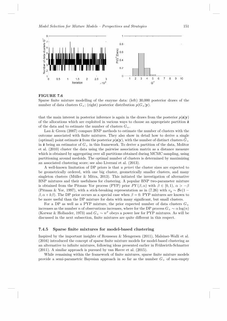
Model Selection for Mixture Models – Perspectives and Strategies 151
FIGURE 7.6Sparse finite mixture modelling of the enzyme data: (left) 30,000 posterior draws of thenumber of data clusters G+; (right) posterior distribution p(G+|y).
that the main interest in posterior inference is again in the draws from the posterior p(z|y)of the allocations which are exploited in various ways to choose an appropriate partition zof the data and to estimate the number of clusters G+.
Lau & Green (2007) compare BNP methods to estimate the number of clusters with theoutcome associated with finite mixtures. They also show in detail how to derive a single(optimal) point estimate z from the posterior p(z|y), with the number of distinct clusters G+in z being an estimator of G+ in this framework. To derive a partition of the data, Molitoret al. (2010) cluster the data using the pairwise association matrix as a distance measurewhich is obtained by aggregating over all partitions obtained during MCMC sampling, usingpartitioning around medoids. The optimal number of clusters is determined by maximizingan associated clustering score; see also Liverani et al. (2013).
A well-known limitation of DP priors is that a priori the cluster sizes are expected tobe geometrically ordered, with one big cluster, geometrically smaller clusters, and manysingleton clusters (Müller & Mitra, 2013). This initiated the investigation of alternativeBNP mixtures and their usefulness for clustering. A popular BNP two-parameter mixtureis obtained from the Pitman–Yor process (PYP) prior PY (β, α) with β ∈ [0, 1), α > −β(Pitman & Yor, 1997), with a stick-breaking representation as in (7.26) with vg ∼ Be(1 −β, α+ kβ). The DP prior occurs as a special case when β = 0. PYP mixtures are known tobe more useful than the DP mixture for data with many significant, but small clusters.
For a DP as well as a PYP mixture, the prior expected number of data clusters G+increases as the number n of observations increases, where for the DP process G+ ∼ α log(n)(Korwar & Hollander, 1973) and G+ ∼ nβ obeys a power law for PYP mixtures. As will bediscussed in the next subsection, finite mixtures are quite different in this respect.
7.4.5 Sparse finite mixtures for model-based clusteringInspired by the important insights of Rousseau & Mengersen (2011), Malsiner-Walli et al.(2016) introduced the concept of sparse finite mixture models for model-based clustering asan alternative to infinite mixtures, following ideas presented earlier in Frühwirth-Schnatter(2011). A similar approach is pursued by van Havre et al. (2015).
While remaining within the framework of finite mixtures, sparse finite mixture modelsprovide a semi-parametric Bayesian approach in so far as the number G+ of non-empty

152 Handbook of Mixture Analysis
mixture components used to generate the data is not assumed to be known in advance,but random, as already discussed in Section 7.3.3. The basic idea of sparse finite mixturemodelling is to deliberately specify an overfitting finite mixture model with too many com-ponents G. Sparse finite mixtures stay within the common finite mixture framework byassuming a symmetric Dirichlet prior η ∼ DG (e0) on the weight distribution; however, thehyperparameter e0 of this prior is selected such that superfluous components are emptiedautomatically during MCMC sampling and sparse solutions with regard to the number G+of clusters are induced through the prior on the weight distribution. This proposal leads to asimple Bayesian framework where a straightforward MCMC sampling procedure is appliedto jointly estimate the unknown number of non-empty data clusters G+ with the remainingparameters.
As discussed in Section 7.3.3, for such a mixture model, the number G of compo-nents does not reflect the number of data clusters, as many components will remain un-used. Following Nobile (2004), Malsiner-Walli et al. (2016) derive the posterior distributionP(G+ = g|y), g = 1, . . . , G, of the number G+ of data clusters from the MCMC output ofthe allocations z. Therefore, for each iteration m of MCMC sampling, all components g towhich some observations have been assigned are identified from z(m) and the correspondingnumber of non-empty components is considered:
G(m)+ = G−
G∑g=1
I(n(m)g = 0),
where, for g = 1, . . . , G, n(m)g =
∑ni=1 I(z
(m)i = g) is the number of observations allocated
to component g, and I(·) denotes the indicator function. The posterior distribution P(G+ =g|y), g = 1, . . . , G, is then estimated by the corresponding relative frequency.
The number of clusters G+ can be derived as a point estimator from this distribution,for example, the posterior mode estimator G+ that maximizes the (estimated) posteriordistribution P(G+ = g|y). This happens to be the most frequent number of clusters visitedduring MCMC sampling. The posterior mode estimator appears to be sensible in the presentcontext when adding very small clusters hardly changes the marginal likelihood. This makesthe posterior distribution P(G+ = g|y) extremely right-skewed, and other point estimatorssuch as the posterior mean are extremely sensitive to prior choices, as noted by Nobile(2004). However, under a framework where sparse finite mixtures are employed for densityestimation, very small components might be important and other estimators of G+ mightbe better justified.
An alternative way to summarize clustering based on sparse finite mixtures is by ex-ploring the posterior draws of the partitions z and determining some optimal partition,such as the partition z minimizing Binder’s loss function. This can be done without theneed to resolve label switching or to stratify the draws with respect to G+. The cardinal-ity G+ of such an optimal partition z is yet another estimator of the number of clusters.The posterior mode estimator G+ and G+ do not necessarily coincide, and differences inthese estimators reflect uncertainty in the posterior distribution over the partition space.As discussed by Frühwirth-Schnatter et al. (2018), the approach of Wade & Gharhamani(2018) to quantifying such uncertainty can be applied immediately to sparse finite mixturemodels.
The appropriate choice of the hyperparameter e0 is important for the application ofthe sparse finite mixture approach in a clustering context. While in a density estimationframework the asymptotic criterion of Rousseau & Mengersen (2011) suggests the choicee0 < r/2, with r being the dimension of θg, this rule is not necessarily a sensible choicefor selecting the number of clusters G+ in a data set of finite size n, as demonstrated fora broad range of mixture models in Malsiner-Walli et al. (2016) and Frühwirth-Schnatter

Model Selection for Mixture Models – Perspectives and Strategies 153
FIGURE 7.7Sparse finite mixture modelling of the enzyme data, displayed as a rug plot. Partition zoptimizing Binder’s loss function. The number of clusters in this partition is equal to three.
& Malsiner-Walli (2018). Indeed, these papers show that values of e0 � r/2 much smallerthan the asymptotic criterion of Rousseau & Mengersen (2011) are needed to identify theright number of clusters, and recommend choosing either very small fixed values such ase0 = 0.001 or applying a hyperprior with e0 ∼ G(ae, be) such that E(e0) = ae/be is verysmall (e.g. e0 ∼ G(1, 200)).
Under the provision that G+ underestimates G, this approach constitutes a simpleand generic strategy for model selection without making use of model selection criteria,RJMCMC, or marginal likelihoods. Applications include Gaussian mixtures as well as mix-tures of Gaussian mixtures (Malsiner-Walli et al., 2017) and sparse mixtures for discrete-valued data (Frühwirth-Schnatter & Malsiner-Walli, 2018). By way of further illustration,the enzyme data (shown earlier in Figure 7.2) are reanalysed using sparse finite mixtures,taking the prior of Richardson & Green (1997) as base measure. The maximum number ofdata clusters is chosen as G = 10 and the hierarchical sparse Dirichlet prior η ∼ DG (e0),e0 ∼ G(1, 200) is applied.
Figure 7.6 shows 30,000 posterior draws of the number of data clusters G+ as wellas the corresponding posterior distribution p(G+|y). The posterior mode estimator yieldsthree clusters with P(G+ = 3|y) = 0.57. Also two clusters are supported with P(G+ =2|y) = 0.19, which is not unexpected in the light of Figure 7.2, showing two (albeit non-Gaussian) data clusters. Due to this misspecification of the component densities the four-cluster solution is equally supported with P(G+ = 4|y) = 0.19. Finally, Figure 7.7 showsthe partition z optimizing Binder’s loss function together with a rug plot of the data. Thenumber of clusters in this partition is equal to three, supporting the choice based on theposterior mode. The resulting clustering nicely captures the three distinct groups of datapoints.

154 Handbook of Mixture Analysis
Relation to BNP methods
The concept of sparse finite mixtures is related in various ways to DP mixtures, discussedin Section 7.4.4. If the weight distribution follows the Dirichlet prior η ∼ DG(α/G) andthe base measure H0 serves as prior for the component parameters (i.e. θg ∼ H0), then, asshown by Green & Richardson (2001), the finite mixture in (7.1) converges to a DP mixturewith mixing distribution H ∼ DP (α,H0) as G increases. This relationship has mainly beenexploited to obtain a finite mixture approximation to the DP mixture. In this sense, thesparse finite Gaussian mixture introduced in Malsiner-Walli et al. (2016) could be seen asan approximation to a DP mixture. Nevertheless, as argued by Malsiner-Walli et al. (2017),it makes sense to stay within the framework of finite mixtures and to consider G as a secondparameter which is held fixed at a finite value, as this provides a two-parameter alternativeto DP mixtures with related properties.
Representations similar to BNP mixtures exist also for finite mixture models under thesymmetric prior η ∼ DG (e0), but are not commonly known, although they shed further lighton the relation between the two model classes. First of all, a stick-breaking representationof the weights η1, η2, . . . , ηG as in (7.26) in terms of a sequence of independently (albeitnot identically) distributed random variables exists also for finite mixtures, with vg ∼Be(e0, (G− g)e0), g = 1, . . . , G− 1, vG = 1; see, for example, Frühwirth-Schnatter (2011).
Second, as already discussed in Section 7.3.1, finite mixture models can be regardedas random partition models and the prior distribution over all random partitions C of nobservations can be derived from the joint (marginal) prior p(z|G) given in (7.19) (see, forexample, Malsiner-Walli et al. (2017)):
p(C|e0, G+) = G!(G−G+)!
Γ(Ge0)Γ(n+Ge0)Γ(e0)G+
∏g:ng>0
Γ(ng + e0).
takes the form of a product partition model as for DP mixtures (see (7.27)) and is invariantto permuting the cluster labels.
Finally, as for BNP mixtures, it is possible to derive the prior predictive distributionp(zi|z−i), where z−i denotes all indicators excluding zi. Let G−i+ be the number of non-empty clusters implied by z−i, and let n−ig , g = 1, . . . , G−i+ , be the corresponding clustersizes. Then the probability that zi is assigned to an existing cluster g is given by
P(zi = g|z−i, n−ig > 0) =n−ig + e0
n− 1 + e0G,
which is closely related to (7.28), in particular if e0 = α/G and G increases. However, theprior probability that zi creates a new cluster with zi ∈ I = {g|n−ig = 0} is equal to
P(zi ∈ I|z−i) =e0(G−G−i+ )n− 1 + e0G
, (7.30)
and is quite different from (7.29). In particular, for e0 independent of G, this probabilitynot only depends on e0, but also increases with G. Hence a sparse finite mixture model canbe regarded as a two-parameter model, where both e0 and G influence the prior expectednumber of data clusters G+, which is determined for a DP mixture solely by α. Furthermore,the prior probability (7.30) of creating new clusters decreases as the number G−i+ of non-empty clusters increases, as opposed to DP mixtures where this probability is constant andto PYP mixtures where this probability increases. Hence, sparse finite mixtures are usefulfor clustering data that arise from a moderate number of clusters that does not increase asthe number of data points n increases.

Model Selection for Mixture Models – Perspectives and Strategies 155
7.5 Concluding RemarksThe issue of selecting the number of mixture components has always been contentious, bothin frequentist and Bayesian terms, and this chapter has reflected on this issue by presentinga wide variety of solutions and analyses. The main reason for the difficulty in estimatingthe order G of a mixture model is that it is a poorly defined quantity, even when settingaside identifiability and label switching aspects. Indeed, when considering a single sampleof size n truly generated from a finite mixture model, there is always a positive probabilitythat the observations in that sample are generated from a subset of the components ofthe mixture of size G+ rather than from all components G. As shown by the asymptoticresults in Chapter 4, the issue goes away as the sample size n goes to infinity (provided Gremains fixed), but this does not bring a resolution to the quandary of whether or not G isestimable. In our opinion, inference should primarily bear on the number of data clustersG+, since the conditional posterior distribution of G given G+ mostly depends on the priormodelling and very little on the data. Without concluding like Larry Wasserman (on his nowdefunct Normal Deviate blog) that “mixtures, like tequila, are inherently evil and shouldbe avoided at all costs”, we must acknowledge that the multifaceted uses of mixture modelsimply that the estimation of a quantity such as the number of mixture components shouldbe impacted by the purpose of modelling via finite mixtures, as for instance through theprior distributions in a Bayesian setting.


Bibliography
Akaike, H. (1974). A new look at the statistical model identification. IEEE Transactionson Automatic Control 19, 716–723.
Banfield, J. D. & Raftery, A. E. (1993). Model-based Gaussian and non-Gaussianclustering. Biometrics 49, 803–821.
Baudry, J.-P. (2015). Estimation and model selection for model-based clustering with theconditional classification likelihood. Electronic Journal of Statistics 9, 1041–1077.
Baudry, J.-P., Maugis, C. & Michel, B. (2012). Slope heuristics: Overview and imple-mentation. Statistics and Computing 22, 455–470.
Baudry, J.-P., Raftery, A. E., Celeux, G., Lo, K. & Gottardo, R. (2010). Combin-ing mixture components for clustering. Journal of Computational and Graphical Statistics19, 332–353.
Berger, J. (1985). Statistical Decision Theory and Bayesian Analysis. New York: Springer-Verlag, 2nd ed.
Berger, J. & Jefferys, W. (1992). Sharpening Ockham’s razor on a Bayesian strop.American Statistician 80, 64–72.
Berkhof, J., van Mechelen, I. & Gelman, A. (2003). A Bayesian approach to theselection and testing of mixture models. Statistica Sinica 13, 423–442.
Bertoletti, M., Friel, N. & Rastelli, R. (2015). Choosing the number of componentsin a finite mixture using an exact integrated completed likelihood criterion. Metron 73,177–199.
Besag, J. (1989). A candidate’s formula: A curious result in Bayesian prediction.Biometrika 76, 183.
Biernacki, C., Celeux, G. & Govaert, G. (2000). Assessing a mixture model for clus-tering with the integrated completed likelihood. IEEE Transactions on Pattern Analysisand Machine Intelligence 22, 719–725.
Biernacki, C., Celeux, G. & Govaert, G. (2010). Exact and Monte Carlo calcula-tions of integrated likelihoods for the latent class model. Journal of Statistical PlanningInference 140, 2991–3002.
Binder, D. A. (1978). Bayesian cluster analysis. Biometrika 65, 31–38.
Birgé, L. & Massart, P. (2001). Gaussian model selection. Journal of the EuropeanMathematical Society 3, 203–268.
Birgé, L. & Massart, P. (2007). Gausian model selection. Probability Theory and RelatedFields 138, 33–73.
157

158 Handbook of Mixture Analysis
Bouveyron, C., Côme, E. & Jacques, J. (2015). The discriminative functional mixturemodel for a comparative analysis of bike sharing systems. Annals of Applied Statistics 9,1726–1760.
Box, G. E. P. (1976). An application of the Laplace method to finite mixture distributions.Journal of the American Statistical Association 71, 791–799.
Bozdogan, H. (1987). Model selection and Akaike’s information criterion (AIC): Thegeneral theory and its analytical extensions. Psychometrika 52, 345–370.
Cappé, O., Robert, C. P. & Rydén, T. (2002). Reversible jump MCMC convergingto birth-and-death MCMC and more general continuous time samplers. Journal of theRoyal Statistical Society, Series B 65, 679–700.
Casella, G., Robert, C. P. & Wells, M. T. (2004). Mixture models, latent variablesand partitioned importance sampling. Statistical Methodology 1, 1–18.
Celeux, G., Chrétien, S., Forbes, F. & Mkhadri, A. (2001). A component-wise EMalgorithm for mixtures. Journal of Computational and Graphical Statistics 10, 697–712.
Celeux, G., Forbes, F., Robert, C. P. & Titterington, D. M. (2006). Devianceinformation criteria for missing data models. Bayesian Analysis 1, 651–674.
Celeux, G. & Soromenho, G. (1996). An entropy criterion for assessing the number ofclusters in a mixture model. Journal of Classification 13, 195–212.
Chen, R. & Liu, J. S. (1996). Predictive updating methods with application to Bayesianclassification. Journal of the Royal Statistical Society, Series B 58, 397–415.
Chib, S. (1995). Marginal likelihood from the Gibbs output. Journal of the AmericanStatistical Association 90, 1313–1321.
Chopin, N. (2002). A sequential particle filter method for static models. Biometrika 89,539–552.
Chopin, N. & Robert, C. P. (2010). Properties of nested sampling. Biometrika 97,741–755.
Côme, E. & Latouche, P. (2015). Model selection and clustering in stochastic blockmodels based on the exact integrated complete data likelihood. Statistical Modelling 6,564–589.
Dacunha-Castelle, D. & Gassiat, E. (1997). The estimation of the order of a mixturemodel. Bernoulli 3, 279–299.
Dacunha-Castelle, D. & Gassiat, E. (1999). Testing the order of a model using locallyconic parametrization: Population mixtures and stationary ARMA processes. Annals ofStatistics 27, 1178–1209.
De Iorio, M. & Robert, C. P. (2002). Discussion of “Bayesian measures of modelcomplexity and fit”, by Spiegelhalter et al. Journal of the Royal Statistical Society, SeriesB 64, 629–630.
Dellaportas, P. & Papageorgiou, I. (2006). Multivariate mixtures of normals withunknown number of components. Statistics and Computing 16, 57–68.

Bibliography 159
DiCiccio, T. J., Kass, R. E., Raftery, A. & Wasserman, L. (1997). ComputingBayes factors by combining simulation and asymptotic approximations. Journal of theAmerican Statistical Association 92, 903–915.
Drton, M. & Plummer, M. (2017). A Bayesian information criterion for singular models.Journal of the Royal Statistical Society, Series B 79, 1–18.
Figueiredo, M. & Jain, A. K. (2002). Unsupervised learning of finite mixture models.IEEE Transactions on Pattern Analysis and Machine Intelligence 24, 381–396.
Fraley, C. & Raftery, A. E. (2002). Model-based clustering, discriminant analysis, anddensity estimation. Journal of the American Statistical Association 97, 611–631.
Frühwirth-Schnatter, S. (1995). Bayesian model discrimination and Bayes factors forlinear Gaussian state space models. Journal of the Royal Statistical Society, Series B 57,237–246.
Frühwirth-Schnatter, S. (2001). Markov chain Monte Carlo estimation of classical anddynamic switching and mixture models. Journal of the American Statistical Association96, 194–209.
Frühwirth-Schnatter, S. (2004). Estimating marginal likelihoods for mixture andMarkov switching models using bridge sampling techniques. Econometrics Journal 7,143–167.
Frühwirth-Schnatter, S. (2006). Finite Mixture and Markov Switching Models. NewYork: Springer-Verlag.
Frühwirth-Schnatter, S. (2011). Dealing with label switching under model uncertainty.In Mixture Estimation and Applications, K. Mengersen, C. P. Robert & D. Titterington,eds., chap. 10. Chichester: Wiley, pp. 193–218.
Frühwirth-Schnatter, S. (2018). Applied Bayesian Mixture Mod-elling. Implementations in MATLAB using the package bayesf Version 4.0.https://www.wu.ac.at/statmath/faculty-staff/faculty/sfruehwirthschnatter/.
Frühwirth-Schnatter, S., Grün, B. & Malsiner-Walli, G. (2018). Contributedcomment on article by Wade and Gharamani. Bayesian Analysis 13, 601–603.
Frühwirth-Schnatter, S. & Malsiner-Walli, G. (2018). From here to infinity –sparse finite versus Dirichlet process mixtures in model-based clustering. Preprint,arXiv:1706.07194.
Frühwirth-Schnatter, S. & Pyne, S. (2010). Bayesian inference for finite mixturesof univariate and multivariate skew normal and skew-t distributions. Biostatistics 11,317–336.
Gassiat, E. (2002). Likelihood ratio inequalities with applications to various mixtures.Annales de l’Institut Henri Poincaré – Probabilités et Statistiques 38, 887–906.
Gassiat, E. & van Handel, R. (2013). Consistent order estimation and minimal penalties.IEEE Transactions on Information Theory 59, 1115–1128.
Gelfand, A. & Dey, D. (1994). Bayesian model choice: Asymptotics and exact calcula-tions. Journal of the Royal Statistical Society, Series B 56, 501–514.

160 Handbook of Mixture Analysis
Gelfand, A. & Smith, A. (1990). Sampling based approaches to calculating marginaldensities. Journal of the American Statistical Association 85, 398–409.
Gelman, A. & Meng, X. (1998). Simulating normalizing constants: From importancesampling to bridge sampling to path sampling. Statistical Science 13, 163–185.
Green, P. J. (1995). Reversible jump MCMC computation and Bayesian model determi-nation. Biometrika 82, 711–732.
Green, P. J. & Richardson, S. (2001). Modelling heterogeneity with and without theDirichlet process. Scandinavian Journal of Statistics 28, 355–375.
Hansen, B. (1992). The likelihood ratio test under non-standard conditions: Testing theMarkov switching model of GNP. Journal of Applied Econometrics 7, S61–S82.
Keribin, C. (2002). Consistent estimation of the order of mixture models. Sankhya, SeriesA 62, 49–66.
Keribin, C., Brault, V., Celeux, G. & Govaert, G. (2015). Estimation and selectionfor the latent block model on categorical data. Statistics and Computing 25, 1201–1216.
Korwar, R. M. & Hollander, M. (1973). Contributions to the theory of Dirichletprocesses. Annals of Probability 1, 705–711.
Lange, K. (1999). Numerical Analysis for Statisticians. New York: Springer-Verlag.
Lau, J. W. & Green, P. J. (2007). Bayesian model-based clustering procedures. Journalof Computational and Graphical Statistics 16, 526–558.
Lee, J. & Robert, C. (2016). Importance sampling schemes for evidence approximationin mixture models. Bayesian Analysis 11, 573–597.
Lee, K., Marin, J.-M., Mengersen, K. & Robert, C. (2009). Bayesian inference onmixtures of distributions. In Perspectives in Mathematical Sciences I: Probability andStatistics, N. N. Sastry, M. Delampady & B. Rajeev, eds. Singapore: World Scientific, pp.165–202.
Lee, S. X. & McLachlan, G. J. (2013). EMMIXuskew: An R package for fitting mixturesof multivariate skew t-distributions via the EM algorithm. Journal of Statistical Software55, 1–22.
Liverani, S., Hastie, D. I., Papathomas, M. & Richardson, S. (2013). PReMiuM:An R package for profile regression mixture models using Dirichlet processes. Preprint,arXiv:1303.2836.
Malsiner-Walli, G., Frühwirth-Schnatter, S. & Grün, B. (2016). Model-basedclustering based on sparse finite Gaussian mixtures. Statistics and Computing 26, 303–324.
Malsiner-Walli, G., Frühwirth-Schnatter, S. & Grün, B. (2017). Identifying mix-tures of mixtures using Bayesian estimation. Journal of Computational and GraphicalStatistics 26, 285–295.
Marin, J.-M., Mengersen, K. & Robert, C. (2005). Bayesian modelling and inferenceon mixtures of distributions. In Handbook of Statistics, C. R. Rao & D. Dey, eds., vol. 25.New York: Springer-Verlag, pp. 459–507.

Bibliography 161
McLachlan, G. (1987). On bootstrapping the likelihood ratio test statistic for the numberof components in a normal mixture. Applied Statistics 36, 318–324.
McLachlan, G. & Peel, D. (2000). Finite Mixture Models. New York: Wiley.
Meng, X. & Wong, W. (1996). Simulating ratios of normalizing constants via a simpleidentity: A theoretical exploration. Statistica Sinica 6, 831–860.
Miller, J. W. & Harrison, M. T. (2018). Mixture models with a prior on the numberof components. Journal of the American Statistical Association 113, 340–356.
Molitor, J., Papathomas, M., Jerrett, M. & Richardson, S. (2010). Bayesian profileregression with an application to the National Survey of Children’s Health. Biostatistics11, 484–498.
Müller, P. & Mitra, R. (2013). Bayesian nonparametric inference – why and how.Bayesian Analysis 8, 269–360.
Nadif, M. & Govaert, G. (1998). Clustering for binary data and mixture models – choiceof the model. Applied Stochastic Models and Data Analysis 13, 269–278.
Neal, R. (1999). Erroneous results in “Marginal likelihood from the Gibbs output”. Tech.rep., University of Toronto.
Nobile, A. (2004). On the posterior distribution of the number of components in a finitemixture. Annals of Statistics 32, 2044–2073.
Nobile, A. & Fearnside, A. (2007). Bayesian finite mixtures with an unknown numberof components: The allocation sampler. Statistics and Computing 17, 147–162.
Pitman, J. & Yor, M. (1997). The two-parameter Poisson-Dirichlet distribution derivedfrom a stable subordinator. Annals of Probability 25, 855–900.
Rau, A., Maugis-Rabusseau, C., Martin-Magniette, M.-L. & Celeux, G. (2015).Co-expression analysis of high-throughput transcriptome sequencing data with Poissonmixture models. Bioinformatics 31, 1420–1427.
Richardson, S. & Green, P. (1997). On Bayesian analysis of mixtures with an unknownnumber of components (with discussion). Journal of the Royal Statistical Society, SeriesB 59, 731–792.
Rissanen, J. (2012). Optimal Estimation of Parameters. Cambrdige: Cambridge UniversityPress.
Robert, C. P. (2007). The Bayesian Choice. New York: Springer.
Robert, C. P. & Casella, G. (2004). Monte Carlo Statistical Methods. New York:Springer-Verlag, 2nd ed.
Roeder, K. (1990). Density estimation with confidence sets exemplified by superclustersand voids in galaxies. Journal of the American Statistical Association 85, 617–624.
Roeder, K. & Wasserman, L. (1997). Practical Bayesian density estimation using mix-tures of normals. Journal of the American Statistical Association 92, 894–902.
Rousseau, J. & Mengersen, K. (2011). Asymptotic behaviour of the posterior distribu-tion in overfitted mixture models. Journal of the Royal Statistical Society, Series B 73,689–710.

162 Handbook of Mixture Analysis
Schwartz, L. (1965). On Bayes procedures. Zeitschrift für Wahrscheinlichkeitstheorie undverwandte Gebiete 4, 10–26.
Schwarz, G. (1978). Estimating the dimension of a model. Annals of Statistics 6, 461–464.
Sethuraman, J. (1994). A constructive definition of Dirichlet priors. Statistica Sinica 4,639–650.
Skilling, J. (2007). Nested sampling for Bayesian computations. Bayesian Analysis 1,833–859.
Spiegelhalter, D. J., Best, N. G., Carlin, B. P. & van der Linde, A. (2002).Bayesian measures of model complexity and fit. Journal of the Royal Statistical Society,Series B 64, 583–639.
Tessier, D., Schoenauer, M., Biernacki, C., Celeux, G. & Govaert, G. (2006).Evolutionary latent class clustering of qualitative data. Tech. Rep. RR-6082, INRIA.
van Havre, Z., White, N., Rousseau, J. & Mengersen, K. (2015). OverfittingBayesian mixture models with an unknown number of components. PLoS ONE 10,e0131739.
Wade, S. & Gharhamani, Z. (2018). Bayesian cluster analysis: Point estimation andcredible balls (with discussion). Bayesian Analysis 13, 559–626.
Wallace, C. & Freeman, P. (1987). Estimation and inference via compact coding.Journal of the Royal Statistical Society, Series B 49, 241–252.
Watanabe, S. (2009). Algebraic Geometry and Statistical Learning Theory. Cambridge:Cambridge University Press.
Wyse, J., Friel, N. & Latouche, P. (2017). Inferring structure in bipartite networksusing the latent block model and exact ICL. Network Science 5, 45–69.
Yang, Y. (2005). Can the strengths of AIC and BIC be shared? A conflict between modelidentification and regression estimation. Biometrika 92, 937–950.
Zeng, H. & Cheung, Y.-M. (2014). Learning a mixture model for clustering with thecompleted likelihood minimum message length criterion. Pattern Recognition 47, 2011–2030.
Zhang, Z., Chan, K. L., Wu, Y. & Chen, C. (2004). Learning a multivariate Gaussianmixture model with the reversible jump MCMC algorithm. Statistics and Computing 14,343–355.