Model reduction tools for nonlinear structural dynamics

Slaats, P.M.A.; de Jongh, J.; Sauren, A.A.H.J.

Published in:Computers and Structures

Published: 01/01/1995

Document VersionPublisher’s PDF, also known as Version of Record (includes final page, issue and volume numbers)

Please check the document version of this publication:

• A submitted manuscript is the author's version of the article upon submission and before peer-review. There can be important differencesbetween the submitted version and the official published version of record. People interested in the research are advised to contact theauthor for the final version of the publication, or visit the DOI to the publisher's website.• The final author version and the galley proof are versions of the publication after peer review.• The final published version features the final layout of the paper including the volume, issue and page numbers.

Link to publication

Citation for published version (APA):Slaats, P. M. A., Jongh, de, J., & Sauren, A. A. H. J. (1995). Model reduction tools for nonlinear structuraldynamics. Computers and Structures, 54(6), 1155-1171.

General rightsCopyright and moral rights for the publications made accessible in the public portal are retained by the authors and/or other copyright ownersand it is a condition of accessing publications that users recognise and abide by the legal requirements associated with these rights.

• Users may download and print one copy of any publication from the public portal for the purpose of private study or research. • You may not further distribute the material or use it for any profit-making activity or commercial gain • You may freely distribute the URL identifying the publication in the public portal ?

Take down policyIf you believe that this document breaches copyright please contact us providing details, and we will remove access to the work immediatelyand investigate your claim.

Download date: 13. Jun. 2018

Compurm & Srrucrures Vol. 54, No. 6, pp. II55-I 171. 1995 Copyright 0 1995 Elsevier Science Ltd

Printed in Great Britain. All riahts reserved > Pergamon

MODEL REDUCTION TOOLS FOR NONLINEAR STRUCTURAL DYNAMICS

P. M. A. Slaats, J. de Jongh and A. A. H. J. Sauren

Department of Mechanical Engineering, Eindhoven University of Technology, P.O. Box 513, 5600 MB Eindhoven. The Netherlands

(Received 27 July 1993)

Abstract-Three mode types are proposed for reducing nonlinear dynamical system equations, resulting from finite element discretizations: tangent modes, modal derivatives, and newly added static modes. Tangent modes are obtained from an eigenvalue problem with a momentary tangent stiffness matrix. Their derivatives with respect to modal coordinates contain much beneficial reduction information. Three approaches to obtain modal derivatives are presented, including a newly introduced numerical way. Direct and reduced integration results of truss examples show that tangent modes do not describe the nonlinear system sufficiently well, whereas combining tangent modes with modal derivatives and/or static modes provides much better reduction results.

1. INTRODUCTION

Direct integration of a system of nonlinear dynamical equations of a finite element model often requires large computation times, despite the increase of computer capacities in the last decades. Therefore, the application of reduction techniques, where the large number of finite element degrees of freedom is reduced to a smaller set of new system coordinates, is still of interest. A corresponding new set of basis vectors can be chosen, forming a second stage of discretization.

Among many publications on reduction tech- niques, Noor [l] and Idelsohn and Cardona [2] in their introduction, present a summary of several reduction methods in nonlinear structural mechanics. For a successful two-stage discretization, a proper selection of the basis vectors is of great importance. The ideal set of basis vectors is one which maximizes the quality of the results and minimizes both the computation times for the reduced system integration and the efforts to obtain these modes.

The present paper focuses on a reduction technique that is based on gathering modes from the initial state of the structure. Once better insight into the merits of the presented types of modes is obtained, these modes can also be updated or incremented for other time instances. However, in the authors’ opinion, first a good understanding of the various types of modes is important, before involving the updating or incre- menting of the modes in the reduced integration process. The presented work is meant as a contri- bution in order to enable optimization of the selection of the basis vectors for a specific time instant (in this paper, i.e. the initial state of the structure), but this

can be generalized to all states at which the mode sets are updated or incremented.

The system of nonlinear dynamical equations of a finite element model is made up of momentum equations, strain-displacement relations as well as boundary conditions and initial conditions. Restrict- ing ourselves to systems without damping, the set of, say N, differential equations to be solved can be denoted as

W(t) = Q(t) - GMt)), (1)

where M is the mass matrix, q(t) a column matrix, containing the N nodal displacements, G(q(t)) a column matrix containing the internal nodal forces and Q(t) a column matrix with the external nodal forces, given as explicit functions of time and satisfying the user supplied dynamic boundary conditions. This set of nonlinear differential equations in combination with the kinematic boundary conditions and the initial conditions

s(t =O)=q,, 4(t = 0) = v, (2)

describe the behaviour of the discretized structural system. In this paper, we only consider geometrical nonlinearities. Generalization to material non- linearities does not imply complications for the presented derivations. The N system equations can be reduced, by substitution of

s(t) = 90 + rq(l), (3)

CAS 54,bK 11.55

1156 P. M. A. Slaats et al.

where P is a reduction matrix, of size N * R, where R is usually much smaller than N, and where q(t) contains R new unknowns. The column with displacements qo, that is q at time t = t,, contains the displacements corresponding to the point in time where the reduction matrix is computed, i.e. the initial state of the structure in this paper. The columns of the reduction matrix are modes, and each mode is multiplied by a corresponding modal coordinate, gathered in column 9.

Substituting eqn (3) in (1) and premultiplying with the transposed reduction matrix gives the resulting nonlinear reduced system

where i?@(t) + G(q, + ‘pii) = at ), (4)

1ci=Y7MY, e=Y’rG, Q=PTQ.

An overbar denotes a quantity in the reduced system. The columns of the reduction matrix may consist

of tangent modes. As will be shown in Section 2, these are the eigenvectors obtained by solving an eigen- value problem of the system that is linearized at a certain time instant, where the tangent stiffness matrix is used. For large displacements, these tangent modes often do not describe the system sufficiently well, so some new vectors, called second-order terms which themselves consist of so-called modal deriva- tives, can be computed and added to the existing set of tangent modes in the reduction matrix. In Section 3, three ways to calculate these modal derivatives are described: two ways based on differentiation of the eigenvalue problem (with or without mass consider- ations), and a third newly introduced way by variation of one of the modal coordinates and creating an additional eigenvalue problem. In Section 4, the application of static modes to the reduction process comes into the picture. Static modes are the steady state solutions of the originally nonlinear dynamic system, and they depend on the external loads applied to the system. Static modes are obtained by an incremental Newton-Raphson iteration procedure, where inertia terms are not considered. The results of two truss problems, one with 13 degrees of freedom and one with 39 degrees of freedom, are presented in Section 5. The solutions of several reduction try-outs are compared to the results of direct integration of the original non-re- duced system. Computation times are compared as well. Conclusions are provided in Section 6.

2. REDUCTION OF THE SYSTEM EQUATIONS BY USING TANGENT MODES

As has been explained in the previous section, the reduction matrix in this paper is determined at the

t In this paper radial eigenfrequencies are called eigenfre- quencies.

initial state of the system with displacements qo.

Around these displacements the system is linearized using the tangent stiffness matrix at time t = t,, so

Tangent modes are determined from the eigenvalue problem

(K,-wiM)$,,=O, for p = l,..., N. (5)

If we fill Y with tangent modes corresponding to the P lowest eigenfrequenciest o,,, we have a linear approximation of displacements q in the ordinary modal corodinates c(~ (p = 1, . , P), which will be rather good in the neighbourhood of the starting displacements qo. In this case, the column of reduced coordinates, Q, only consists of the ordinary modal coordinates, a,, @ = 1, , P), as in linear systems. Equation (3) can be written as

p= I

where P = R, the number of new unknowns.

3. ADDITION OF MODAL DERIVATIVES TO THE SET OF NEW BASIS VECTORS

For nonlinear systems with large displacements, the tangent stiffness matrix is likely to change a lot. This means that also the tangent modes change as a function of the nodal displacements, and as a matter of fact they also change as a function of the modal coordinates c(~. So (with all N tangent modes), eqn (6) can be written as

q - qo = Aq = i &,(q)ap) = ‘f’& “=I

(7)

We now assume that we can develop Aq around its starting configuration Aq = 0 into a second-order Taylor series

The derivatives of the nodal displacements are com- puted by using eqn (7)

(10)

Reduction of nonlinear structural dynamics equations 1157

At the considered displacements, q,,, the column with ordinary modal coordinates consists of zeros, (x = 0. The derivatives of eqns (9) and (10) are at this point

!$!(a =O)=&(q=q,) P

(11)

~(a=O)=$$(q=qo)+~(q=qo). (12) P 7 P ,

If the stiffness matrix would not be a function of the displacements, the derivatives of the tangent modes with respect to the modal coordinates in eqns (9) and (10) would disappear and just an ordinary tangent mode, I&,, would remain. However, if the system equations contain nonlinearities, the reduction matrix can be filled with P ordinary tangent modes and R - P derivatives as defined in eqn (12). Then the column q with R reduced coordinates is filled with P ordinary modal coordinates, ELI, (p = 1, . , P), and R - P kind of quadratic ordinary modal coordinates, so the dimension of different elements of ij is not the same. Equation (7) can now be written as

($~+~)(q=q,)...]WPa. (13)

Three alternative ways of determining the modal derivatives, &j&x,,, are presented in the next three subsections.

3.1. Analytical approach including mass consideration

Based on ideas of Idelsohn and Cardona [2-41, the background of an analytical approach to obtain modal derivatives is mathematically further explored here.

To find a modal derivative, say a&/&x,,, we differ- entiate the eigenvalue problem, eqn (5) with respect to the ordinary modal coordinate OL,,

(K-WjM)$($-$&. (14)

The derivative of the tangent stiffness matrix with respect to the pth ordinary modal coordinate is determined numerically by using the varied stiffness matrix

The magnitude of&x,, must be chosen consciously in order to obtain an accurate numerical solution for this derivative: it should be small enough for the accuracy of the numerical solution for the derivative of the tangent stiffness matrix, but on the other hand it cannot be too small, because of computer round-off errors.

Idelsohn and Cardona [2-41 only consider the case where one unique tangent mode corresponds to the eigenfrequency w,. As a suggestion to further gener- alization, we shall describe the case where two tangent modes correspond to one and the same eigenfrequency w,. Later on, we shall also restrict ourselves to the case where one tangent mode belongs to w,.

If two tangent modes (4, and $,+ ,) belong to CO,, the rank of the matrix (K - o:M) is N - 2. The nullspace of this matrix consists of the two tangent modes belonging to w,. According to [5], the general solution of the modal derivative may be written as the sum of the homogeneous solution of eqn (14) that is the solution of eqn (14) where the elements of the column in the right- hand side are set to zero, and a particular solution

where

(17)

for arbitrary fii, i = 1,2. A comment on the parameters 8, is given at the end of this section. A particular solution of the modal derivative will only be found if the right-hand side of eqn (14) satisfies two conditions, because the column space of (K -w;‘M) consists of N -2 inde- pendent columns. Therefore the right-hand side of eqn (14) has only N - 2 independent elements. To find these conditions and to find a particular solution, the original unknowns, W,iaEP Ipar are represented with respect to another basis, resulting in a new column {a+,/&,}‘. This corresponds to a multiplication of the column with the new unknowns by a square N * N matrix T, resulting in the column with the original unknowns

(18)

1158 P. M. A. Slaats et al.

We may choose the transformation matrix T as follows:

T=

0

1 k . 1 N

. (19)

The transformation matrix, T, is the same as the unit matrix except for its k th and Ith column, which are chosen to be equal to the tangent modes & and

4 r + , , respectively. We choose k such that the kth

element of +,, i&}kr is unequal to zero and 1 such that (4, + , }, is unequal to zero, otherwise T would be singular. Except for these two restrictions on k and 1, choices fork and 1 are arbitrary. Substitution of eqn (18) into eqn (14) and premultiplying with T’ gives

=TT($M-g)$,. (20)

Independent of the solution of the transformed modal derivatives, {a&/&x,)‘, the kth and Ith equation of eqn (20) are respectively

For tangent modes that are normalized with re- spect to the mass matrix, these equations can be simplified

(23)

(24)

If the tangent modes belonging to w, do not satisfy eqn (24), an inconsistency exists. Using eqn (23) (20) can be rewritten. The k th and Ith equations of eqn (20) may be left out, because the kth and Ith columns and rows of the matrix in the left-hand side of eqn (20), T’(K - ofM)T, only contain zeros

=T:W#d:-I)$ (25) P

Here, Tt is the transformation matrix where the kth and lth column are omitted and {&$,j&,,}; is the column containing the transformed modal derivatives where the kth and Ith elements are omitted. These elements are undefined. They are multiplied with the tangent modes, see eqns (18) and (19) which are also taken into account in the homogeneous solution, as shown in eqn (17). Therefore, we may choose the k th and Ith element of the transformed modal derivative equal to zero. Then eqn (25) may be rewritten as

where {.}* is a column with its kth and lth element omitted, and (.)* is a matrix with its kth and Ith columns and rows removed. A solution of eqn (26),

{@#a,};, can now be determined, and the total column {~~~/~~,,}’ can be obtained by inserting the chosen zero elements for its k th and Ith element. By using eqn (18) an N-dimensional particular solution {~~,/~a~)par is obtained, to be substituted into eqn

(16). This method can easily be generalized to the case

where S tangent modes belong to w,. Of course, we can also only consider the case where one unique tangent mode corresponds to one eigenfrequency w,, like Idelsohn and Cardona[2-41 do. Then, one equation remains [eqn (23)], by which the derivative of the squared eigenfrequency, dwj/&, can be obtained.

Finally, a remark concerning the parameters fi, is appropriate now. If the reduction matrix, Y, contains modal derivatives of the two tangent modes 4, and

Q, r+ I) that belong to one and the same eigenfrequency 0,. and if these tangent modes are also taken into account in Y, the free to chosen values b,, do not matter, because for each p,, (i = 1, 2), the columns of Y span the same subspace. Therefore we may choose the parameters 8, equal to zero, and only the determination of the particular solution remains.

3.2. Analytical approach excluding mass consideration

It can be shown that multiplication of all system masses by a factor “J results in a decrease of the modal derivatives with the same factor y. So multiplication of all masses by the same factor does not influence the shape of the modal derivative.

Related to this property, a simplification of the calculation of the modal derivatives is proposed by

Reduction of nonlinear structural dynamics equations 1159

Idelsohn and Cardona [2-41 by neglecting all inertia terms. Then, eqn (14) becomes

(27)

The inverse of the tangent stiffness matrix exists because the rigid body motions are prevented. Although this approximation seems rather crude, it will be shown that this kind of ‘static’ modal deriva- tive gives practically the same results as when the modal derivative is determined as in the previous

section. In [3], it is stated that these approximated modal

derivatives possess the following kind of symmetry

(28)

Because of this symmetry property, for this method the number of modal derivative evaluations could be reduced in comparison with both the method de- scribed in the previous section and the method to be described in the next section.

3.3. Numerical approach to determine modal derivatives

A new approach to obtain modal derivatives is presented now. To determine a numerical solution, the pth ordinary modal coordinate is varied and its influence on the tangent stiffness matrix K is computed by calculating K(q,) and K(q,+ &,pSolP). With these two stiffness matrices, two eigenvalue problems are calculated and the modal derivative can be determined from

84, aa,’

+,(qo + 4p*ap) - 9rho) *cr, (29)

In ew (2% 4&d and 4,h + &i$,) denote tangent modes corresponding to the tangent stiffness matrix K(q,) and K(q, + $,,&,,), respectively. This method requires, besides recomputing the stiffness matrix for each da,, also the calculation of a second eigenvalue problem. The increment 6aP should be small enough for the accuracy of the numerical

solution for the modal derivatives, but on the other hand it can be too small, because of computer round-off errors.

4. APPLICATION OF STATIC MODES TO THE REDUCTION PROCESS

Another new aspect presented in this paper is the linear combination of tangent modes and their de- rivatives on the one hand, and static modes on the other hand in the set of new basis vectors and the corresponding new system coordinates.

Static modes are determined by neglecting inertia terms in the system equations of motion, where an applied static load causes the structure to deform. The nonlinear set of algebraic equations looks as follows [see eqn (1), where Q is no longer time- dependent]

Q - G(q) = 0. (30)

The internal force column is nonlinear in the displace- ments. A Newton-Raphson iteration process can be applied to solve this system. In order to enable convergence to the correct root of the nonlinear

system, the incremental load approach [6] is appropriate. Small load increments reduce the total number of iterations required for convergence per increment. The solution q of the iteration process can be used as an additional column in the reduction matrix Y.

5. TRUSS PROBLEMS: NUMERICAL EXAMPLES

In order to test the concepts presented in the previous sections, simple truss problems are con- sidered. For the geometrical discretization, linear displacement fields between the ends of the truss elements are used. General two-dimensional truss elements with elastic constitutive behaviour are con- sidered. For the strain-displacement relation, the Green-Lagrange strain measure is adopted. A lumped inertia approach (see e.g. [7]) is employed. The classical explicit fifth-order Runge-Kutta inte- gration method with adaptive step size control has been implemented for the computations.

6 8

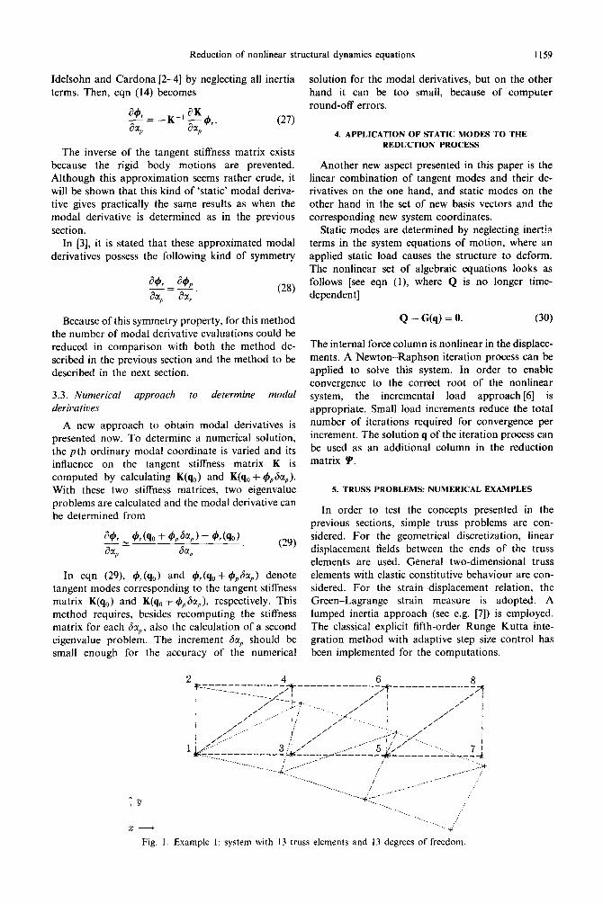
Fig. 1. Example 1: system with 13 truss elements and 13 degrees of freedom.

1160 P. M. A. Slaats er al.

In the two examples that are shown, the common physical properties of all truss elements are: cross- sectional area 0.0025 m2, Young’s modulus 2.1 x IO” N/m* and mass density 7800 kg/m3.

5.1. Truss problem with 13 degrees of freedom

ln a first example, the truss element structure shown in Fig. 1 is considered. The system consists of eight nodes and 13 truss elements. The initial nodal displacements and velocities equal zero, and the x- and y-displacements of the lower left node and the x-displacement of the upper left node are suppressed, in order to prevent rigid body motions. At the upper right node (i.e. node 8) a constant external force of 2 x lo-’ N is applied in the negative y-direction. The length of the total structure in its initial state amounts to 3 m and the width equals 1 m.

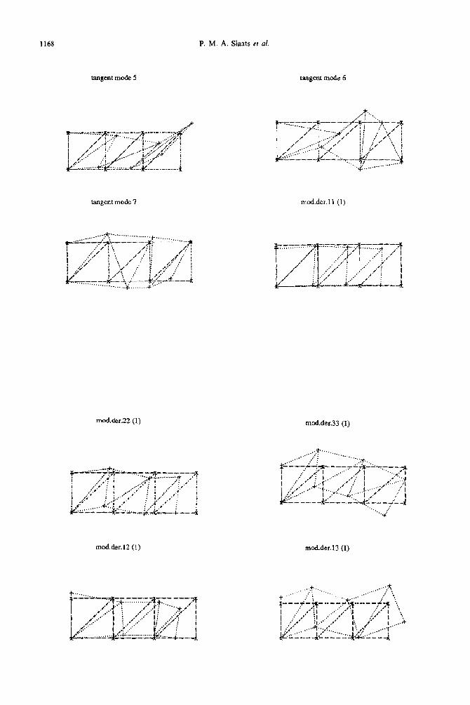
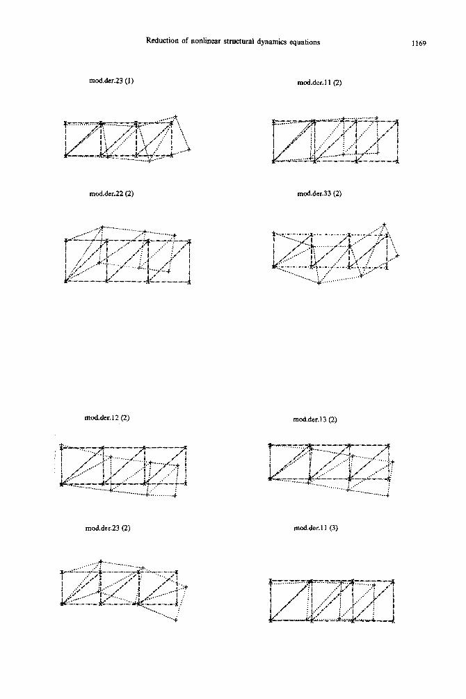
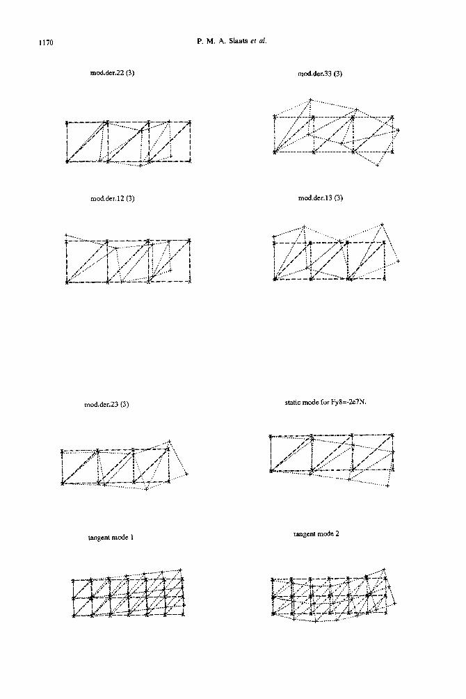
In Table 1, a summary of the numerical tests is given. A collection of the tangent modes, their deriva- tives and static modes that are used as new basis vectors in the reduction process are visualized in the Appendix.t In order to get a neat visualization, the modes that are shown in the Appendix are scaled (for visualization only!) by a constant factor. This factor is obtained by letting the maximum value of the

t Note that in the Appendix the titles in the modal derivative plots have been abbreviated as mod.der.ij(k), where i and j correspond to i and j in at,/&,,, and where k corresponds to the used approach to determme the modal derivative, k = 1: analytical approach including mass con- sideration (Section 3. I); k = 2: analytical approach exclud- ing mass consideration (Section 3.2); and k = 3: numerical approach (Section 3.3).

column change into half the minimum undeformed element length.

In Fig. 2, the displacement in the y-direction of the eight node is shown for reduced integration solutions where only tangent modes are used in the new set of basis vectors. It must be remarked that the solution obtained with 13 tangent modes turns out to be exactly the same as the solution of direct integration of the original nonreduced system, which may be expected, since the original system contains 13 degrees of freedom. Furthermore, it can be concluded from Fig. 2 that by adding more tangent modes to the new set of basis vectors, the reduced solution still gives poor results and the computation times get worse, as can be noted from Table 1. All computation times of this example are compared to the compu- tation time that is needed for direct integration of the original, nonreduced system (see the right-hand column in Table 1).

In order to get some insight about what tangent modes are dominant for this nonlinear structural dynamics system, the modal coordinates in the case of reduction by a set of 13 tangent modes are displayed as functions of time in Fig. 3. In this case, for a proper comparison, the columns of the re- duction matrix are scaled according to the visualiza- tion scaling. In this way, the modal coordinate amplitudes may be compared in Fig. 3.

From Fig. 3, it appears that the modal coordinates corresponding to the first and the third tangent modes have the largest amplitudes for this nonlinear system, whereas the other modal coordinate amplitudes are of the same low order. In the next test simulations, at most three tangent modes will be

Table 1. Mode sets for reduction and relative computation effort

Total number No. of No. of No. of Relative Type of line in figure of modes tangent modes second-order tangents static modes computation time

Figure 2

1 I 0 0 0.062 5 5 0 0 0.463 9 9 0 0 1.108

13 13 0 0 1.921

Figure 4 3 3 0 0 0.229 3 2 1 0 0.320 3 2 0 I 0.379

xxx 3 1 1 I 0.264 Direct 1.000

integration

Figure 5 -~ (a) - 6 3 3 0 0.980

(b) 6 3 3 0 0.951 _.~._ (c) 6 3 3 0 0.956

Direct I .ooo integration

Figure 6 (1) ~- 9 3 6 0 1.357 (2) 9 3 6 0 1.404

-‘-’ (3) 9 3 6 0 1.365 Direct 1.000

integration

t

-0.2

-1

-1.5

-2

-2.:

i ;‘

i-

I ; 0

Reduction of nonlinear structural dynamics equations 1161

0.005 0.01 0.015 0.02 0.025 0.03 0.035 ( ,4

time [s]

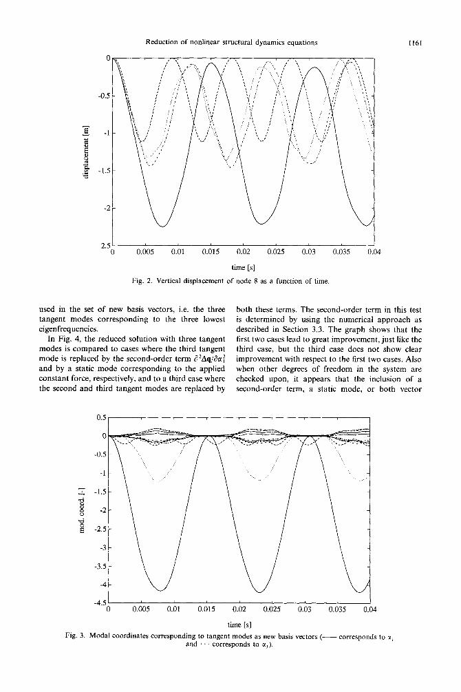
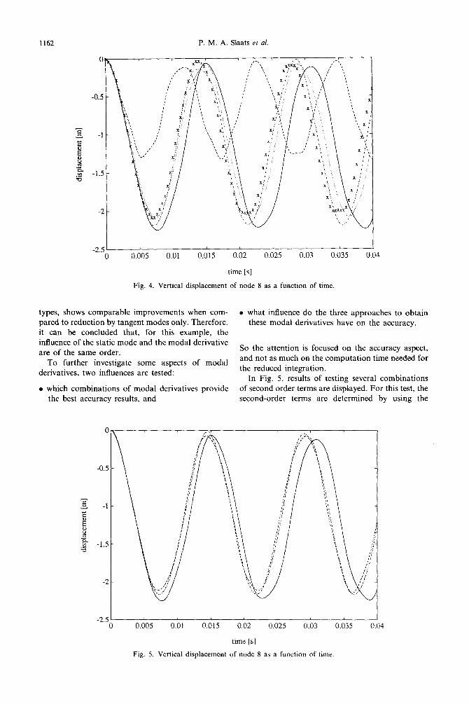
Fig. 2. Vertical displacement of node 8 as a function of time

used in the set of new basis vectors, i.e. the three tangent modes corresponding to the three lowest eigenfrequencies.

In Fig. 4, the reduced solution with three tangent modes is compared to cases where the third tangent mode is replaced by the second-order term d*Aq/&xi and by a static mode corresponding to the applied constant force, respectively, and to a third case where the second and third tangent modes are replaced by

both these terms. The second-order term in this test is determined by using the numerical approach as described in Section 3.3. The graph shows that the first two cases lead to great improvement, just like the third case, but the third case does not show clear improvement with respect to the first two cases. Also when other degrees of freedom in the system are checked upon, it appears that the inclusion of a second-order term, a static mode, or both vector

-2.5 -

..L

0 0.005 0.01 0.015 0.02 0.025 0.03 0.035 0.04

time [s]

Fig. 3. Modal coordinates corresponding to tangent modes as new basis vectors (-- corresponds to c(, and corresponds to c(,).

1162 P. M. A. Slaats et al.

0

-0.5

z -1 B

i ,m .s -1.5

-2

-2.5 ,- 0 0.005 0.01 0.015 0.02 0.025 0.03 0.035 14

time [s] Fig. 4. Vertical displacement of node 8 as a function of time.

types, shows comparable improvements when com- pared to reduction by tangent modes only. Therefore, it can be concluded that, for this example, the influence of the static mode and the modal derivative are of the same order.

To further investigate some aspects of modal derivatives, two influences are tested:

l which combinations of modal derivatives provide the best accuracy results, and

l what influence do the three approaches to obtain these modal derivatives have on the accuracy.

So the attention is focused on the accuracy aspect, and not as much on the computation time needed for the reduced integration.

In Fig. 5, results of testing several combinations of second order terms are displayed. For this test, the second-order terms are determined by using the

-2.5 ’ I

0 0.005 0.01 0.015 0.02 0.025 0.03 0.035 0.04

time [s]

Fig. 5. Vertical displacement of node 8 as a function of time.

Reduction of nonlinear structural dynamics equations 1163

time [s]

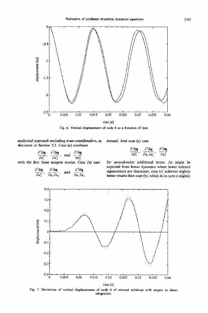
Fig. 6. Vertical displacement of node 8 as a function of time.

analytical approach excluding mass consideration, as instead. And case (c) discussed in Section 3.2. Case (a) combines \ I

d2Aq alAq

aa: ' aa:' and ?!!

aa:

a2Aq

acl:’

uses

a 2Aq a’Aq

acr,’ sol:

with the first three tangent modes. Case (b) uses for second-order additional terms. As might be

PAq a2Aq and a2Aq

expected from linear dynamics where lower indexed

,a:’ ati, aa,' aa, da3 eigenvectors are dominant, case (c) achieves slightly better results than case (b), which in its turn is slightly

time [s]

Fig. 7. Deviations of vertical displacements of node 8 of reduced solutions with respect to direct integration.

1164 P. M. A. Slaats et al.

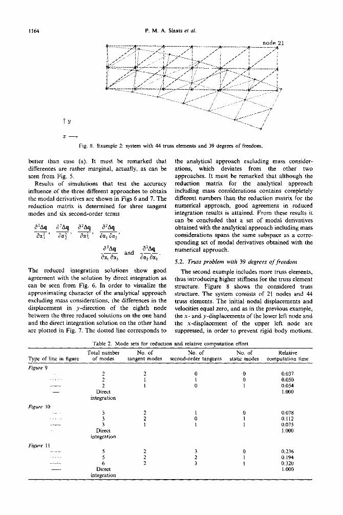
Fig. 8. Example 2: system with 44 truss elements and 39 degrees of freedom.

better than case (a). It must be remarked that differences are rather marginal, actually, as can be seen from Fig. 5.

Results of simulations that test the accuracy influence of the three different approaches to obtain the modal derivatives are shown in Figs 6 and 7. The reduction matrix is determined for three tangent modes and six second-order terms

a2Aq and a2Aq

au, au, aa,acc,’

The reduced integration solutions show good agreement with the solution by direct integration as can be seen from Fig. 6. In order to visualize the approximating character of the analytical approach excluding mass considerations, the differences in the displacement in y-direction of the eighth node between the three reduced solutions on the one hand and the direct integration solution on the other hand are plotted in Fig. 7. The dotted line corresponds to

the analytical approach excluding mass consider- ations, which deviates from the other two approaches. It must be remarked that although the reduction matrix for the analytical approach including mass considerations contains completely different numbers than the reduction matrix for the numerical approach, good agreement in reduced integration results is attained. From these results it can be concluded that a set of modal derivatives obtained with the analytical approach including mass considerations spans the same subspace as a corre- sponding set of modal derivatives obtained with the numerical approach.

5.2. Truss problem with 39 degrees of freedom

The second example includes more truss elements, thus introducing higher stiffness for the truss element structure. Figure 8 shows the considered truss structure. The system consists of 21 nodes and 44 truss elements. The initial nodal displacements and velocities equal zero, and as in the previous example, the x- and y-displacements of the lower left node and the x-displacement of the upper left node are suppressed, in order to prevent rigid body motions.

Table 2. Mode sets for reduction and relative computation effort

Total number No. of No. of No. of Relative

Type of line in figure of modes tangent modes second-order tangents static modes computation time

Figure 9 2 2 0 0 0.037

..,.. 2 1 I 0 0.050 2 I 0 1 0.054

Direct 1 .OOo

integration

Figure 10 3 2 I 0 0.078 3 2 0 I 0.112 3 1 1 1 0.075

Direct 1.000 integration

Figure 1 I 5 2 0 0.236 5 2 : 1 0.194

_._._ 6 2 3 I 0.320 Direct 1.000

integration

Reduction of nonlinear structural dynamics equations 1165

-0.6

E -0.8

E g -1

Y 4 B

-1.2

-1.4

-1.6

-1.8

0.005 0.01 0.015 0.02 0.025 0.03 0.035

time [s]

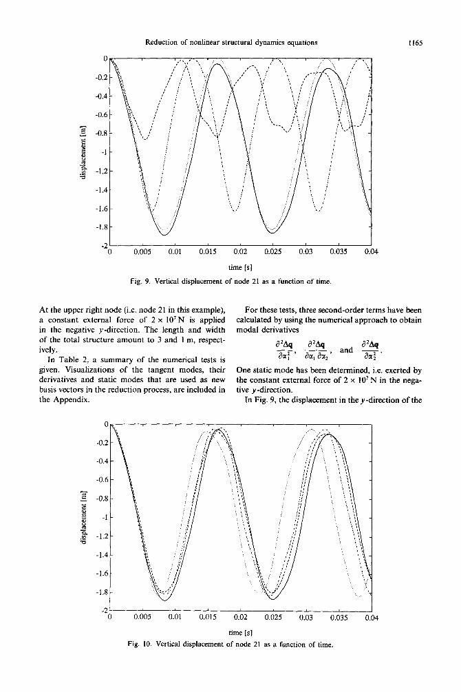
Fig. 9. Vertical displacement of node 21 as a function of time.

At the upper right node (i.e. node 21 in this example), a constant external force of 2 x IO’N is applied in the negative y-direction. The length and width of the total structure amount to 3 and 1 m, respect- ively.

In Table 2, a summary of the numerical tests is given. Visualizations of the tangent modes, their derivatives and static modes that are used as new basis vectors in the reduction process, are included in the Appendix.

For these tests, three second-order terms have been calculated by using the numerical approach to obtain modal derivatives

a2Aq d2Aq -- au: ' au, au,'

and azL\q au: One static mode has been determined, i.e. exerted by the constant external force of 2 x IO’ N in the nega- tive y-direction.

In Fig. 9, the displacement in the y-direction of the

-0.4 -

-0.6 -

z -0.8 - E i -I-

z? S? G

-1.2 -

-1.4 -

-1.6 -

-1.8 -

-2 ’ 0 0.005 0.01 0.015 0.02 0.025 0.03 0.035

time [s]

Fig. 10. Vertical displacement of node 21 as a function of time.

1166 P. M. A. Slaats et al.

0.005 0.01 0.015 0.02 0.025 0.03 0.035

time [s]

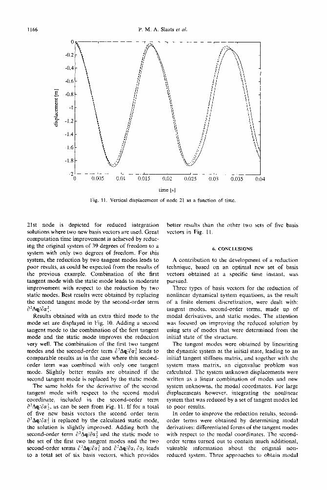
Fig. 11. Vertical displacement of node 21 as a function of time.

2lst node is depicted for reduced integration solutions where two new basis vectors are used. Great computation time improvement is achieved by reduc- ing the original system of 39 degrees of freedom to a system with only two degrees of freedom. For this system, the reduction by two tangent modes leads to poor results, as could be expected from the results of the previous example. Combination of the first tangent mode with the static mode leads to moderate improvement with respect to the reduction by two static modes. Best results were obtained by replacing the second tangent mode by the second-order term d*Aq/&;.

Results obtained with an extra third mode to the mode set are displayed in Fig. 10. Adding a second tangent mode to the combination of the first tangent mode and the static mode improves the reduction very well. The combination of the first two tangent modes and the second-order term a2Aq/8af leads to comparable results as in the case where this second- order term was combined with only one tangent mode. Slightly better results are obtained if the second tangent mode is replaced by the static mode.

The same holds for the derivative of the second tangent mode with respect to the second modal coordinate, included in the second-order term a2Aq/&:, as can be seen from Fig. 11. If for a total of five new basis vectors the second order term a’Aq/&xi is replaced by the calculated static mode, the solution is slightly improved. Adding both the second-order term d’Aq/&i and the static mode to the set of the first two tangent modes and the two second-order terms c?2Aq/&j and a2Aq/&, dr, leads to a total set of six basis vectors, which provides

better results than the other two sets of five basis vectors in Fig. 11.

6. CONCLUSIONS

A contribution to the development of a reduction technique, based on an optimal new set of basis vectors obtained at a specific time instant, was pursued.

Three types of basis vectors for the reduction of nonlinear dynamical system equations, as the result of a finite element discretization, were dealt with: tangent modes, second-order terms, made up of modal derivatives, and static modes. The attention was focused on improving the reduced solution by using sets of modes that were determined from the initial state of the structure.

The tangent modes were obtained by linearizing

the dynamic system at the initial state, leading to an initial tangent stiffness matrix, and together with the system mass matrix, an eigenvalue problem was calculated. The system unknown displacements were written as a linear combination of modes and new system unknowns, the modal coordinates. For large displacements however, integrating the nonlinear system that was reduced by a set of tangent modes led to poor results.

In order to improve the reduction results, second- order terms were obtained by determining modal derivatives: differentiated forms of the tangent modes with respect to the modal coordinates. The second- order terms turned out to contain much additional, valuable information about the original non- reduced system. Three approaches to obtain modal

Reduction of nonlinear structural dynamics equations 1167

derivatives were presented. Two analytical ap- improve the reduced solutions. Comparable proaches, one with and one without mass consider- influence, not to such a great extent though, can be ations, originated from ideas of Idelsohn and perceived by the introduction of static modes. Cardona (1985). These methods were mathematically Addition of both modal derivatives and static modes fully evaluated in this paper. In addition, a third and to the set of tangent modes is also possible, but newly introduced numerical approach was presented does not always show satisfactorily cumulative in this paper. improvement.

Reduced integration results for these three methods were compared also. A slight difference in reduced integration results occurred between both analytical approaches: the neglecting of mass only has a small influence on the result. The reduced integration results for the analytical approach including mass considerations showed very good agreement with the numerical approach introduced in this paper. Although their reduction matrices contained completely different numbers, the reduction matrix of the analytical approach including mass considerations was concluded to span the same subspace as the reduction matrix of the approach introduced in this paper.

Finally, it must be remarked that the efforts to obtain the tools for reduction are much less than the integration efforts themselves. The positive influence on the computation times of the presented nonlinear dynamics reduction technique was clearly illustrated by the numerical examples.

REFERENCES

1.

2.

3.

Another new aspect in this paper is the combi- nation of tangent modes and their derivatives with static modes in the linear combination of new basis vectors and corresponding new system coordinates. Numerical test simulations were executed for truss problems with large displacements. The solution obtained by direct integration qf the nonreduced system was used to check the results of the many reduced integration try-outs.

4.

5.

6.

From the numerical tests, it can be concluded that the use of tangent modes only, cannot be accepted. Modal derivatives (or second-order terms) should be added to the new set of basis vectors in order to

I.

A. K. Noor, Recent advances in reduction methods for nonlinear problems. Comput. Strucr. 13, 31-44 (1981). S. R. Idelsohn and A. Cardona, A reduction method for nonlinear structural dynamic analysis. Compur. Meth. Appl. Mech. Engng 49, 253-219 (1985). S. R. Idelsohn and A. Cardona, Computational strategies for nonlinear and fracture mechanics problems. Comput. Struct. 20, 203-210 (1985). S. R. Idelsohn and A. Cardona, Recent advances in reduction methods in nonlinear structural dynamics. In Proceedings of the Second Infernational Conference on: Recent Advances in Slructural dynamics (Edited by M. Petyt and H. F. Wolfe), Vol. II, pp. 475-482. University of Southampton (1984). G. Strang, Linear Algebra and ifs Applications. Harcourt Brace Jovanovich, Orlando, FL (1988). 0. C. Zienkiewicz and R. L. Taylor, The Finite Elemenf Method, Vol. 1: Basic Formulalion and Linear Problems. Vol. 2: Solid and Fluid Mechanics; Dynamics and Non - linearity. McGraw-Hill, New York (1989). A. Cardona and M. Geradin, Modelling of super- elements in mechanism analysis. Int. J. Numer. Merh. Engng 32, 1565-1593 (1991).

tangent mode 1

APPENDIX: VISUALIZATION OF BASIS VECTORS

tangent mode 2

tangent mode 3 tangent mode 4

1168 P. M. A. Slaats et al.

tangent mode 5 tangent mode 6

tangent mode 7

mod.der.22 (1)

mod.der.11 (1)

mod.der.33 (1)

mod.der.13 (1)

Reduction of nonlinear structural dynamics equations 1169

mod.der.23 (1)

mod.der.22 (2)

mod.der.12 (2)

mod.der.23 (2)

mod.der.11 (2)

mod.der.33 (2)

mod.der. 13 (2)

mod.der. 11 (3)

1170 P. M. A. Slaats ef al.

mod&r.22 (3) mod.der.33 (3)

mod.der.12 (3)

mod.der.23 (3)

tangent mode 1

mod.der.13 (3)

static mode for Fy8=-2e7N.

tangent mode 2

Reduction of nonlinear structural dynamics equations

mod.der. 11 (2) maLder.12 (2)

mod.der.22 (2) static mode for Fy21=-Ze7N.

AS 546-L