Model Performance Evaluation and Scenario Analysis · PDF fileModel Performance and Scenario...

Model Performance and Scenario Analysis Tool Tutorial 1

EPA/600/EPA/600/B‐16/080 May 2016

Model Performance Evaluation and Scenario Analysis (MPESA) Tutorial


By

Yusuf Mohamoud, Ph.D., P.E. National Exposure Research Laboratory

Office of Research and Development United States Environmental Protection Agency

RTP, North Carolina

U.S. Environmental Protection Agency Office of Research and Development

Washington, DC 20460


DISCLAIMER

This tutorial document has been reviewed by the National Exposure Research

Laboratory (NERL), U.S. Environmental Protection Agency (USEPA) and has been

approved for publication. The model performance evaluation and scenario analysis tool

has not been tested extensively with diverse data sets. The author and the U.S.

Environmental Protection Agency are not responsible and assume no liability

whatsoever for any results or any use made of the results obtained from this program,

nor for any damages or litigation that result from the use of this tool for any purpose.

Mention of trade names or commercial products does not constitute endorsement or

recommendation for use.

Citation:

Mohamoud Y.M. Model Performance Evaluation and Scenario Analysis (MPESA) Tutorial. US EPA Office of Research and Development, Washington DC, EPA/600/B-16/080, 2016


ACKNOWLEDGEMENTS

Acknowledgments are due to Xueyao Yang and Matthew Panunto for their participation in the development of the model performance evaluation and scenario analysis tool.

ABSTRACT

This tool consists of two parts: model performance evaluation and scenario analysis (MPESA). The model performance evaluation consists of two components: model performance evaluation metrics and model diagnostics. These metrics provides modelers with statistical goodness-of-fit measures that capture magnitude only, sequence only, and combined magnitude and sequence errors. The performance measures include error analysis, coefficient of determination, Nash-Sutcliffe efficiency, and a new weighted rank method. These performance metrics only provide useful information about the overall model performance. Note that MPESA is based on the separation of observed and simulated time series into magnitude and sequence components. The separation of time series into magnitude and sequence components and the reconstruction back to time series provides diagnostic insights to modelers. For example, traditional approaches lack the capability to identify if the source of uncertainty in the simulated data is due to the quality of the input data or the way the analyst adjusted the model parameters. This report presents a suite of model diagnostics that identify if mismatches between observed and simulated data result from magnitude or sequence related errors. MPESA offers graphical and statistical options that allow HSPF users to compare observed and simulated time series and identify the parameter values to adjust or the input data to modify. The scenario analysis part of the tool provides quantitative metrics on how model simulated scenario results differ from the baseline results and what impact these differences may have on aquatic organisms and their habitats (e.g., increased flood and drought frequency).


TABLE OF CONTENTS Please insert report number and logo here ............................................. Error! Bookmark not defined.

ACKNOWLEDGEMENTS ............................................................................................................................. 4

1.0 Introduction .......................................................................................................................................... 7

2.0 Model Performance Evaluation and Scenario Analysis Tool .......................................................... 8

2.1. Data requirement ............................................................................................................................ 8

2.2 Importing Data ................................................................................................................................. 8

2.3 Model Performance and Diagnostics Tool .................................................................................. 14

2.3.1. Basic Statistical Analysis – Magnitude Only ........................................................................ 15

2.3.2 Visualization and Zooming ........................................................................................................ 16

2.3.3 Diagnostics and Feedback – Magnitude Only ......................................................................... 21

2.3.4 Diagnostics and Feedback Magnitude Only Comparisons .................................................... 29

2.4 Baseline and Scenario Comparison Tool ..................................................................................... 42

2.4.1 Low Flow Analysis– 7Q10 ........................................................................................................... 42


LIST OF FIGURES

Figure 1: Select Tool panel .......................................................................................................... 9 Figure 2: Paired Input Time Series Data .................................................................................. 10

Figure 3: Enter Data Information .............................................................................................. 11

Figure 4: Paste Data Window .................................................................................................... 13

Figure 5: Paired Input Time Series Data Panel with Imported Data .................................... 13

Figure 6: Model Performance and Diagnostics Tool Panel ................................................... 14

Figure 7: Descriptive Statistics Panel ........................................................................................ 15

Figure 8: Error Analysis Panel .................................................................................................... 16

Figure 9: Time Series Plot of Observed and Simulated Data ................................................ 17

Figure 10: Duration Curve ......................................................................................................... 18

Figure 11: Annual and Monthly Panel ..................................................................................... 19

Figure 12: Plotted Time Series of Average/Aggregated Data .............................................. 20

Figure 13: Daily Statistics Panel ................................................................................................ 21

Figure 14: Summary Statistics for Years of Interest ............................................................... 22

Figure 15: Quantile RSR Panel .................................................................................................. 23

Figure 16: NRMSE Plot ............................................................................................................... 24

Figure 17: Baseflow Separation ................................................................................................ 25

Figure 18: Time-series and Duration Curve Plots from Baseflow Separation ..................... 26

Figure 19: Annual Duration Curves .......................................................................................... 27

Figure 20: Calculated Statistics, Flow Duration Curve, and Percentile Values .................... 28

Figure 21: Magnitude Comparison Panel ................................................................................ 30

Figure 22: Frequency Comparison Panel with Optional Plot ................................................ 31

Figure 23: Quantile Comparison Panel .................................................................................... 32

Figure 24: Serial and Cross Correlation Analysis Panel ......................................................... 33

Figure 25: Correlation Analysis Calculated .............................................................................. 35

Figure 26: Correlation Analysis Plotted ................................................................................... 36

Figure 27: Weighted Rank Panel .............................................................................................. 38

Figure 28: Weighted Rank Plot ................................................................................................. 39

Figure 29: Combined Magnitude and Sequence Performance Panel ................................. 40

Figure 30: Baseline and Scenario Comparison Tool............................................................... 43

Figure 31: Low Flow Analysis - 7Q10 Panel ............................................................................. 44


Figure 32: Hydrologic Indicators of Change - Flashiness Panel ........................................... 45

Figure 33: Environmental Flow Calculations Panel................................................................. 46

Figure 34: Indices of Flow Variability - Flow Pulses Panel with Optional Plot .................... 47

1.0 Introduction The Model Performance Evaluation and Scenario Analysis Tool is based on the time series separation and reconstruction (TSSR) paradigm in which observed and simulated time series are separated into magnitude and sequence components. Note that the magnitude component is represented by the duration curve also known as the exceedance probability curve and sequence is separated from the time series and stored for reconstruction applications (Mohamoud, 2014). The tool allows users to paste simulated output data along with observed data for the same corresponding time period, and calculate a suite of model performance measures that compare the two datasets. It also plots a variety of graphs to visually compare the simulated results with the observed data. MPESA consists of two components: Model Performance Evaluation and Diagnostics, and Baseline and Scenario Comparison. The Model Performance Evaluation and Diagnostics provides important insights that facilitate the model calibration process. Although this component provides important insights about model calibration, it is not a model calibration tool because it does not automatically adjust model parameter values or explicitly inform modelers which parameter to adjust manually. The component provides statistical metrics that include error analysis, weighted ranks, and model efficiency. It can also perform calculations to aggregate data values, assess serial correlations between simulated and observed results, and generate time series and duration curve plots. The Baseline and Scenario Comparison component calculates low flow indices (e.g., 7Q10), environmental flow indices, indicators of flow flashiness, and indices of flow variability. These comparisons allow tool users to assess how much a particular index changed from the baseline condition. In addition, it enables environmental managers


and engineers to determine the consequence that these changes have on environmental protection or design of hydraulic structures. Note that this document is a tutorial that guides the user to estimate model performance metrics and visualization tools to facilitate the model calibration effort. As such, this document is not manual that presents detailed information about the methods. 2.0 Model Performance Evaluation and Scenario Analysis Tool 2.1. Data requirement

Tool users must remove all headers/text from the data before pasting it into the “Import Data” window. This can be achieved by removing headers in a word-editing program such as Notepad or the desktop HDFT tool. The tool uses a date, observed time series, and simulated time series columns. It also uses baseline and scenario columns.

The tool works only with tab-separated date and value formats. Please refer to Appendix for sample data format.

Note: The tool removes row numbers with missing data and informs the user about rows with missing values if the values are designated as blank. Example data used: Data source: USGS NWIS Source site name: St. Jones River at Dover, DE Site number: 01483700 Dates used: 01/01/2000 to 12/31/2009

2.2 Importing Data Before running the tool, users are required to paste their data into the tool. This section presents the steps necessary for users to import their data.


Step 1: Open/run the tool. Step 2: The program should display a main window with four tabs (Select Tool, Paired Input Time Series Data, Model Performance and Diagnostics Tool, and Baseline and Scenario Comparison Tool). To access the Model Performance and Diagnostics components of the tool, select the “Model Performance and Diagnostics Tool” radio button from the Select Tool panel [Figure 1].

Figure 1: Select Tool panel

A new window which directs users to the Paired Input Time Series Data tab will appear

[Figure 2].


Figure 2: Paired Input Time Series Data

Step 3: Click the button of the Paired Input Time Series Data Panel to open the “enter data information” window [Figure 3]. Note: Tool users must arrange the columns so that the date is placed in the first, observed data in the second and the simulated data in the third column.


Figure 3: Enter Data Information

To avoid formatting errors, tool users must select the exact date and time format including the date and time separators from the “Enter Data Information” Window.


Step 4: On the “enter data information” window, select the format of the date according to your input data. In this example, MM/DD/YYYY is selected [Figure 3]. Note: In the current example, daily data are used, thus the hour and minute

checkboxes were not selected. If the data are hourly or sub-hourly, check the corresponding hour and minute checkboxes.

Step 5: Enter the correct date and time separators of the imported data. Note that a backslash “/” is used as the date separator in this example. Note: The tool does not work properly if the date separator entered and the date

separator of the pasted data does not match.

Step 6: After the proper date and time formats are selected, click to open the “Paste Data” window [Figure 4].


Figure 4: Paste Data Window

Step 7: Paste the raw data (using Ctrl + V) into the “Paste Data” window [Figure 4]. Note: The data may not import properly if less than 3 columns are pasted into the

import data window

Step 8: Click at the bottom of the window [Figure 4] to bring in the data into the Paired Input Time Series Data table [Figure 5].

Figure 5: Paired Input Time Series Data Panel with Imported Data


Note: For this example data, the observed and simulated data are similar in magnitude but not in sequence. The simulated column is shifted backward by one day to introduce deliberately a sequence error.

2.3 Model Performance and Diagnostics Tool Once data has been properly imported, users can now run the Model Performance and Diagnostics Tool [Figure 6], which evaluates how well the model simulated the observed data. The Model Performance and Diagnostics Tool panel is organized into groups by functionality: Basic Statistical Analysis, Visualization and Zooming, Diagnostics and Feedback, Sequence Only, and Combined Magnitude and Sequence. .

Figure 6: Model Performance and Diagnostics Tool Panel


2.3.1. Basic Statistical Analysis – Magnitude Only Step 1: Click on Model Performance and Diagnostics Tool tab [Figure 6]. Step 2: A statistical summary for the observed and simulated datasets are calculated by

clicking the button [Figure 6].

Figure 7: Descriptive Statistics Panel

Figure 7 shows comparisons of observed and simulated descriptive statistics that include mean, maximum, minimum, standard deviation, variance, coefficient of variation, and skew coefficient. To demonstrate the importance of magnitude and sequence evaluations, even though, the simulated column was shifted backward by one day, all the descriptive statistics for the observed and simulated datasets are equal. This suggests that description statistics capture only magnitude but not sequence differences.


Step 3: For additional model evaluation statistics, click the button [Figure 6] to display the Error Analysis Panel [Figure 8].

Figure 8: Error Analysis Panel

Note: The results of the error analysis show that mean error and percent PBIAS have zero values suggesting that these two statistics only capture magnitude error but not sequence errors. Conversely, the absolute mean error seem to capture both magnitude and sequence errors. 2.3.2 Visualization and Zooming Step 1: The observed and simulated datasets can be viewed by clicking the

button [Figure 6] to display comparisons of observed and simulated time-series data in a plotting environment [Figure 9]. Note: To view the observed and simulated datasets individually, users can click the

radio buttons at the bottom of the window


Figure 9: Time Series Plot of Observed and Simulated Data

Note: The zoomed time series plot shows the backward shift of the simulated time series data. Step 2: A Duration Curve [Figure 10] for the observed and simulated data can be

viewed by clicking shown in [Figure 6].


Figure 10: Duration Curve

Figure 10 shows that the simulated and observed data have the same duration curves or magnitude curves even though the two datasets have time sequence differences (one-day shift). As such, duration curves represent only magnitude components of a time series and are useful only in capturing magnitude related errors. Note that [Figure 10] does not show the effect of the one-day shift or the sequence error.


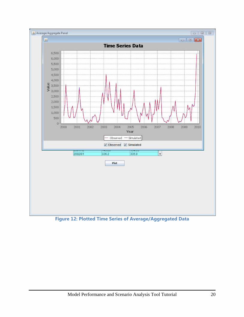
Step 3: Users can aggregate their observed and simulated data to obtain yearly or

monthly sums and averages by clicking the button [Figure 6], which will show the Annual and Monthly Panel [Figure 11]. Users must select their time step and operation of choice from the drop down options prior to clicking the

button. The averaged/aggregated data can then be plotted as a time

series by clicking [Figure 12].

Figure 11: Annual and Monthly Panel

Note: Annual and monthly panel offers only visualization; It does not offer diagnostic guidelines to modelers.


Figure 12: Plotted Time Series of Average/Aggregated Data


2.3.3 Diagnostics and Feedback – Magnitude Only Step 1: Daily statistics can be calculated for both the observed and simulated data by

clicking the button shown in [Figure 6], which opens the Daily Statistics Panel [Figure 13]. Users can then select years of interest and click the Plot Data button to view time series plots or click the Calculate Statistics button to calculate sample statistics for the selected observed and simulated data [Figure 14].

Figure 13: Daily Statistics Panel


Plotting the entire time series (observed and simulated time series) on years by year basis and comparing the observed and simulated hydrographs provides important diagnostic insights that include the identification of outliers in the observed time series data. It also shows the years with hydrograph over-prediction and under-prediction thus alerting the modeler to search for possible answers about the causes of the hydrograph differences.

Figure 14: Summary Statistics for Years of Interest

Note: The lower part of Figure 14 calculates mean, median, standard deviation, and coefficient of variation of observed and simulated data for an average water year.


Step 2: To view the normalized root mean square error for the datasets, click the

button shown in [Figure 6] to bring up the Quantile RSR Panel

[Figure 15]. When the button is selected in the Quantile RSR Panel [Figure 15], the NRMSE results can be viewed for various quantiles in a graph [Figure 16].

Figure 15: Quantile RSR Panel

Note: The normalized root mean square error values that correspond to the 15 exceedances are all zeros. Error values of zeros signify that the data does not have magnitude errors and that this statistic does not capture sequence errors.


Figure 16: NRMSE Plot

Note: NRMSE values of zeros for all exceedance in Figure 16 signify the absence of magnitude errors in the data.

Step 3: Click the button shown in [Figure 6]. A base flow separation window will appear. Upon entering a user specified Base flow index and moving average interval, the base flow and direct flow statistics are calculated for the observed and simulated data [Figure 17].


Figure 17: Baseflow Separation

Note: The first step is to plot the observed total flows with the observed baseflow and examine if the upper baseflow line touches the lower part of the total flow line (Figure 17). If the baseflow line is either too low or too high compared to the total flow line, tool users need to adjust the baseflow index and the moving average interval values until the two lines touch each other at both the rising and the recession limb of the hydrograph. Now that the maximum baseflow index and the smoothing factor are set, tool users need to calibrate the model until the simulated baseflow matches the observed baseflow and the simulated direct runoff matches the observed direct runoff. We assume that observed and simulated direct runoff will automatically match when observed and simulated baseflows match.


Step 4: The calculated baseflow and direct flow statistics can be viewed in a plot [Figure 18] by selecting one or more columns of discharge values and clicking the

button. Alternatively, duration curves of the flow values can be

generated by clicking the button. Note: Users do NOT need to select the data column to plot time-series graph

Figure 18: Time-series and Duration Curve Plots from Baseflow Separation

Figure 18 Simulated total streamflow and direct runoff duration curves.


Step 5: Annual duration curves can be viewed for both the observed and simulated data

by clicking the button [Figure 6]. Step 6: With the Annual Duration Curves Panel now open [Figure 19], users may calculate statistics, create a duration curve, or calculate exceedance values by selecting more than one column of data (by holding the CTRL button) and clicking the

button, button, or button [Figure 19]. The summary statistics for the selected columns will appear as new columns on the left end of the scrollable Annual Duration Curves Panel [Figure 20]. New windows will appear for the duration curve and exceedances values.

Figure 19: Annual Duration Curves


Note Year by year magnitude curve or duration curve comparisons identify the years in which model predictions are relatively poor. These comparisons provide diagnostic guidelines to modelers.

Figure 20: Calculated Statistics, Flow Duration Curve, and Percentile Values

Note: Calculated statistics, duration curve comparisons, and percentile values provide useful diagnostic guidelines to modelers.


2.3.4 Diagnostics and Feedback Magnitude Only Comparisons Step 1: A magnitude comparison of the observed and simulated data can be viewed by clicking the button shown in [Figure 6], which will display the Magnitude Comparison Panel with an option to plot the observed and simulated magnitude values [Figure 21]. This panel will also display the calculated Nash-Sutcliffe Efficiency and R square values between the two datasets. Note that these values are estimated from the entire dataset and offer numerical performance metrics about magnitude component prediction only, but magnitude comparisons alone do not offer diagnostic guidelines to modelers.


Figure 21: Magnitude Comparison Panel

Note: A Nash-Sutcliffe Efficiency of one in Figure 21 means no magnitude errors. Step 2: Frequency comparison plot can be viewed by clicking the

button shown in [Figure 6]. The Frequency Comparison Panel is shown on [Figure 22], with an option to plot the flood frequency at various return periods.


Figure 22: Frequency Comparison Panel with Optional Plot

Note: Frequency comparisons of observed and simulated datasets offer diagnostic guideline of how well the model simulated the annual peak flows. For this example, the magnitudes of the observed and the simulated time series are equal and their peak flow values are equal.

Step 3: Quantile values can be viewed by clicking the button [Figure 6], which will produce a Quantile Comparison Panel [Figure 23] displaying the observed and simulated flow values for each quantile. By clicking the plot button, the quantile values can be viewed in a graph [Figure 23].


Figure 23: Quantile Comparison Panel

Note: Quantile comparisons provide diagnostic guidelines that allow modelers to identify the quantiles whose simulated values are over-predicted or under-predicted in respect to the observed values. Modelers may tie specific processes to specific quantiles so that they can identify and adjust relevant parameter values as part of the model calibration process.


2.3.5 Sequence Comparisons Step 1: Correlation analysis of observed and simulated data can be ran by clicking the

button shown in [Figure 6]. The correlation analysis consists of Serial and Cross Correlation Analysis of observed and simulated datasets [Figure 24].

Figure 24: Serial and Cross Correlation Analysis Panel


Figure 24 compares the cross correlation between observed and simulated data and the serial correlations of the observed and simulated data. Further, this panel calculates Nash-Sutcliffe values between two serial correlations and between the serial correlations and the cross-correlation. The correlation analysis provides diagnostic insights about sequence errors.

Step 2: Users may accept the default input values for maximum number of lags (default value of 20), or they may enter user-specified values. Once acceptable values are

entered, click the button to obtain Nash-Sutcliffe Coefficient values and correlation results [Figure 25].


Figure 25: Correlation Analysis Calculated

Figure 25 shows calculated correlation values and their corresponding Nash-Sutcliffe values. Note that a backward shift of one day for the simulated time series has resulted in a slight decrease in Nash-Sutcliffe values. A decrease in Nash-Sutcliffe between serial and cross correlation indicates the presence of sequence errors in the pairwise comparisons.


Step 3: To plot the results of the correlation analysis, click the button [Figure 26]. A plot window will appear displaying the observed and simulated serial correlation as well as the cross correlation [Figure 26].

Figure 26: Correlation Analysis Plotted

Note that these correlation comparisons capture only sequence errors such as shifts between observed and simulated data. Note that shifts in the precipitation input data, which occurs when precipitation data are not available at-site and is transferred from far away weather stations. In general, when the precipitation input is not aligned with the flow hydrograph, observed and simulated peak flows are not aligned and these miss-alignments introduce a shift, which in turn results in both sequence and magnitude errors. A shift in observed and simulated hydrographs can also be introduced by inaccurate representation of channel characteristics and flow routing through tributary and mainstem channels of a watershed. For example, if Mannings n, channel slope, and storage capacities of the channel are accurately represented, sequence related shift can occur even when precipitation data are available at at-site.


Step 4: Users can also view a rank comparison table of all dataset values by clicking the

button shown in [Figure 6] to open the Weighted

Rank Panel [Figure 27]. By clicking the button, users can view the weighted rank values in a plot environment [Figure 28].

Figure 27: Weighted Rank Panel

Figure 27 shows observed and simulated rank comparisons resulting from one-day backward shift of the simulated column. The percentage of ranks matched in each segment of the duration curve is also shown on the right of Figure 27. Note that the number of data points in each segment has an influence on the segment-specific calculated weighted rank values.


Figure 28: Weighted Rank Plot

Figure 28 shows the percentage of observed and simulated ranks that matched for each segment of the duration curve. An average weighted rank of 0.81 (Figure 27) represents a sequence error caused by a one-day backward shift of the simulated time series. Note that the weighted rank method is the method of choice for sequence related error evaluations. The weighted rank was developed to capture sequence errors only and it does not capture magnitude related errors.


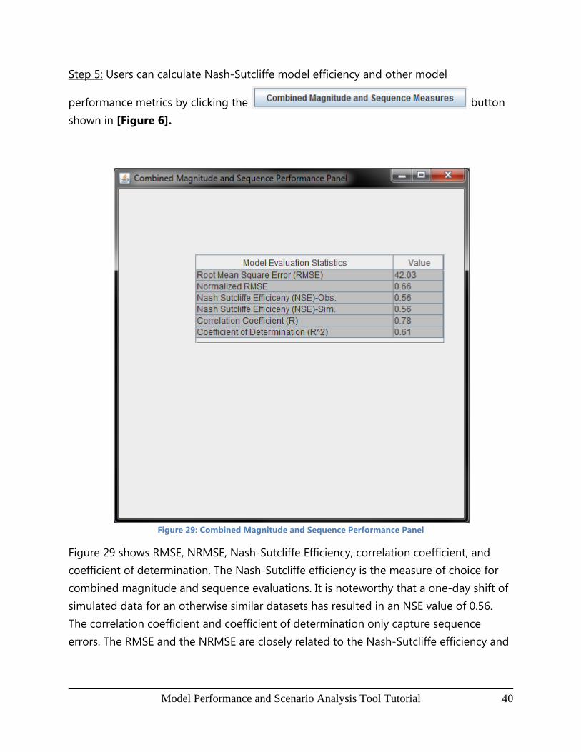
Step 5: Users can calculate Nash-Sutcliffe model efficiency and other model

performance metrics by clicking the button shown in [Figure 6].

Figure 29: Combined Magnitude and Sequence Performance Panel

Figure 29 shows RMSE, NRMSE, Nash-Sutcliffe Efficiency, correlation coefficient, and coefficient of determination. The Nash-Sutcliffe efficiency is the measure of choice for combined magnitude and sequence evaluations. It is noteworthy that a one-day shift of simulated data for an otherwise similar datasets has resulted in an NSE value of 0.56. The correlation coefficient and coefficient of determination only capture sequence errors. The RMSE and the NRMSE are closely related to the Nash-Sutcliffe efficiency and


both can capture magnitude and sequence errors. We recommend the use of NSE in place of RMSE and NRMSE.


2.4 Baseline and Scenario Comparison Tool

The baseline and scenario comparison component does not support model calibration because it does not calculate model performance measures. The Baseline and Scenario Comparison has four components for analyzing input datasets: Low Flow Analysis – 7Q10, Hydrological Indicators of Change – Flashiness, Environmental Flow Calculations, and Indices of Flow Variability – Flow Pulses. Users must first upload their data into the tool (see Section 2.2: Importing Data before proceeding to this portion of the tutorial). 2.4.1 Low Flow Analysis– 7Q10 Step 1: Once data has been properly imported into the tool (see Section 2.2 of the

tutorial), click on to display all Baseline and Scenario Comparison options [Figure 30]. The goal of estimating low flow indices is to quantify the degree to which flow values changed from baseline to scenario and whether such a change violates environmental flow requirements.


Figure 30: Baseline and Scenario Comparison Tool

Step 2: Click the button [Figure 30] to bring up the Low Flow Analysis – 7Q10 panel [Figure 31]. Users can then select any of the three

radio buttons within the panel and click the button to generate results according to a specified flow-averaging period and return interval, explicit flow value, or flow percentile.


Figure 31: Low Flow Analysis - 7Q10 Panel

The goal of estimating low flow indices is to quantify the degree to which flow values change from baseline to scenario and whether such change violates environmental flow requirements.


Step 3: Click on [Figure 30] to view a table of various metrics and index values that describe the relative flashiness of a location based on the provided input [Figure 32].

Figure 32: Hydrologic Indicators of Change - Flashiness Panel

The hydrologic indicators of change assess the effect of urbanization on water quantity and quality. It can also be used to assess the effect of climate change on water quantity and quality.


Step 4: Hydrological indicators such as flow magnitude, rise and fall rates, minimum and maximum conditions, as well as their relative timing within the year can be viewed by

clicking the button shown in [Figure 30] and through navigating the Group tabs

[Figure 33]. Note: Environmental flow calculations assess how flow alterations affect aquatic organisms and their habitat.

Figure 33: Environmental Flow Calculations Panel

Step 5: Another option available to users is the hydrological change detection component, which calculates flow variability of observed and simulated datasets and ranks them according to their varying magnitude thresholds. Click the


button shown in [Figure 30] to generate the Indices of Flow Variability – Flow Pulses panel [Figure 34]. Users also have the option

to create a plot of the hydrological change values by clicking the button [Figure 34].

Figure 34: Indices of Flow Variability - Flow Pulses Panel with Optional Plot

Note: The indices of variability uses median based threshold values to estimate flow alterations caused by urbanization and other anthropogenic disturbances

Model Performance Evaluation and Scenario Analysis · PDF fileModel Performance and Scenario...

Documents

Transcript of Model Performance Evaluation and Scenario Analysis · PDF fileModel Performance and Scenario...