I give permission for public access to my thesis and for any copying

to be done at the discretion of the archives librarian and/or the College

librarian.

Surabhi Gupta ’11

Abstract

The brain is incredibly efficient at storing and searching through large

environments. While we have amassed a burgeoning amounts of data on

the brain regions and neuronal mechanisms involved, we do not under-

stand the framework and processes underlying the cognitive map. This

thesis proposes a novel model of pathfinding using distributed representa-

tions in a hierarchical framework. Compositional rules for generations of

higher-scale locations are recursively defined using Holographic Reduced

Representations [Plate, 1991]. Pathfinding is based on hierarchical search

across the levels of the hierarchy. Locations are retrieved using autoasso-

ciative recall. This model has many salient features and biologically real-

istic features such as automatic generalization, efficient scale-wise search,

robustness and graceful degradation in larger environments.

To test the paradigm of hierarchical spatial reasoning in the brain, I de-

signed and conducted from an event-related potential (ERP) experiment.

During the training phase, the participants were allowed to explore a vir-

tual environment and were encouraged to visualize and remember paths

between different landmarks. During the experiment, subjects are given

a task followed by three spatial maps which appear in succession. For

each map, they are asked to indicate whether it is most relevant to the

path-finding task. Significant differences were found between the evoked

potentials in various conditions which point towards the saliency of a hi-

erarchical representation.

Using Holographic Reduced Representations to Model

Hierarchical Spatial Reasoning

by

Surabhi Gupta

Prof. Audrey Lee-St. John

(Research Advisor)

A thesis submitted in partial fulfillment

of the requirements for the

Degree of Bachelor of Arts with Honors

in Computational Neuroscience.

Mount Holyoke College

South Hadley, Massachussetts

30th April, 2011

Acknowledgements

I would like to express my sincere gratitude to my thesis advisor professor

Audrey, for her unwavering support, patience, inspiration, and knowledge,

for helping me navigate my thesis through the interdisciplinary field of

computational neuroscience. I thank professor Dave Touretzky who pro-

vided the original formulation of the hierarchical navigation problem as an

HRR-based associative retrieval problem and motivating me to pursue it.

I am thankful to Professor Lee Bowie and Lee Spector for insightful

discussions and hard questions, Prof. Paul Dobosh, Prof. Joe Cohen,

Prof. Gary Gillis, Prof. Jane Couperus, Prof. Barbara Lerner, Prof. Lisa

Ballesteros and Prof Sue Barry for their support and encouragement.

I thank Professor Tai Sing Lee for the opportunity to participate in

the Program in Neural Computation at Carnegie Mellon University. I

thank my labmates Anoopum Gupta, Brian Gereke, Timothy Carroll and

Melanie Cox for stimulating discussions. I thank the Center for Neural

Basis of Cognition for funding my summer project.

I’m grateful to the Computer Science and Neuroscience departments at

MHC and the Cognitive Science department at Hampshire for supporting

me in this endeavor.

Last but not the least I would like to thank my parents Dr. Shailendra

Kumar Gupta and Mrs. Padma Gupta for raising me, for their teachings

and for their unconditional support.

Contents

1 Introduction 10

1.1 Discussion of Spatial Knowledge . . . . . . . . . . . . . . . 11

1.2 Related Work . . . . . . . . . . . . . . . . . . . . . . . . . 12

1.3 Contributions . . . . . . . . . . . . . . . . . . . . . . . . . 15

1.4 Structure of Thesis . . . . . . . . . . . . . . . . . . . . . . 15

2 Background & Preliminaries 16

2.1 Background . . . . . . . . . . . . . . . . . . . . . . . . . . 16

2.1.1 Neuroscience background . . . . . . . . . . . . . . . 17

2.1.2 Computer Science background . . . . . . . . . . . . 18

2.1.3 Connectionism . . . . . . . . . . . . . . . . . . . . 19

2.2 Preliminaries . . . . . . . . . . . . . . . . . . . . . . . . . 22

2.2.1 Distributed Representations . . . . . . . . . . . . . 23

2.2.2 Autoassociative Memory . . . . . . . . . . . . . . . 25

2.2.3 Hierarchical Spatial Reasoning . . . . . . . . . . . . 26

3 Pathfinding Framework and Process 28

3.1 Pathfinding Framework . . . . . . . . . . . . . . . . . . . . 29

1

2

3.1.1 Hierarchical Composition of locations . . . . . . . . 30

3.1.2 Auto-associative Memory . . . . . . . . . . . . . . . 32

3.2 Processes . . . . . . . . . . . . . . . . . . . . . . . . . . . 34

3.2.1 Checking for the Goal . . . . . . . . . . . . . . . . 37

3.2.2 Retrieving the next Scale . . . . . . . . . . . . . . . 39

3.2.3 Retrieving the Path . . . . . . . . . . . . . . . . . . 40

3.3 Features of the Algorithm . . . . . . . . . . . . . . . . . . 43

3.4 Analyzing the Process . . . . . . . . . . . . . . . . . . . . 44

4 Extension to Continuous Domain 47

4.1 Extension to Framework . . . . . . . . . . . . . . . . . . . 48

4.1.1 Autoassocaitive Memories . . . . . . . . . . . . . . 49

4.2 Extension to Process . . . . . . . . . . . . . . . . . . . . . 50

4.2.1 Checking for the Goal . . . . . . . . . . . . . . . . 51

4.2.2 Goal Retrieval . . . . . . . . . . . . . . . . . . . . . 51

5 Experiments and Results 52

5.1 Experiments on the Process . . . . . . . . . . . . . . . . . 52

5.2 Autoassociative Memory . . . . . . . . . . . . . . . . . . . 55

5.2.1 Neural Net . . . . . . . . . . . . . . . . . . . . . . 56

5.2.2 Hopfield Net . . . . . . . . . . . . . . . . . . . . . . 61

6 Event Related Potential Experiment 64

6.1 Introduction . . . . . . . . . . . . . . . . . . . . . . . . . . 64

6.2 Methods and Procedures . . . . . . . . . . . . . . . . . . . 65

6.2.1 Training Phase . . . . . . . . . . . . . . . . . . . . 65

3

6.2.2 Experiment Phase . . . . . . . . . . . . . . . . . . 67

6.3 Results and Discussion . . . . . . . . . . . . . . . . . . . . 69

7 Conclusions and Future Work 74

A Derivation of δ(X,A) 77

B Pathfinding Example 79

B.1 Binary Framework Example . . . . . . . . . . . . . . . . . 79

B.2 Continuous Framework Example . . . . . . . . . . . . . . . 86

B.3 Dimensionality . . . . . . . . . . . . . . . . . . . . . . . . 92

List of Figures

2.1 Cortical hierarchy depicting the formation of invariant rep-

resentations in hearing, vision and touch. Reprinted from

“On Intelligence” [Hawkins and Blakeslee, 2004] . . . . . . 18

2.2 Hierarchical Representation of the Environment. The top-

most node is the root node and the three nodes at the lowest

scale are the leaf nodes. Values for depth and scale are in-

dicated on the left. Height of the tree is the depth of a leaf

node . . . . . . . . . . . . . . . . . . . . . . . . . . . . . . 27

3.1 A sample hierarchical framework depicted in graphical form.

Each location at higher scale is composed of the constituting

locations at lower scales. Indexes are indicated next to the

scale number. Note: The edges do not encode any feature

of the spatial environment such as distances etc; they are

merely a conceptual aid and not pointers as typically con-

ceived in computer science. This works to our advantage in

designing a recursive compositional rule. . . . . . . . . . . 30

4

5

3.2 Locations at scale i are merged together to obtain the merged

sequence µ(i+ 1, p). This vector is bound with a key κ(i+

1, p) to obtain the location at scale i+1, λ(i+ 1, p) . . . . . 31

3.3 The Location memory stores all the state vectors and their

associated keys. It stores as many state vectors as size(V)

and as many keys as size(I) . . . . . . . . . . . . . . . . . 33

3.4 The different nodes along one branch of the hierarchy, from

top to bottom, are packed into a sequence and stored in the

packed hierarchy memory. The shaded path pertains to

the vector: κ(1− 5) +κ(1− 5)⊗κ(2− 2) +κ(1− 5)⊗κ(2−

2) ⊗ κ(3 − 1) The number of such vectors is given by the

size of set N, the set of all parents of the leaf nodes . . . . 34

3.5 The Supplementary memory stores superposed expressions

with the keys and the merged vector . . . . . . . . . . . . 35

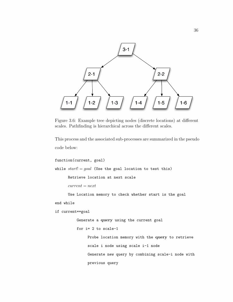
3.6 Example tree depicting nodes (discrete locations) at differ-

ent scales. Pathfinding is hierarchical across the different

scales. . . . . . . . . . . . . . . . . . . . . . . . . . . . . . 36

3.7 Flow chart depicting the various stages of the pathfinding

process . . . . . . . . . . . . . . . . . . . . . . . . . . . . . 37

3.8 Flow chart depicting the various steps involved in checking

for the goal . . . . . . . . . . . . . . . . . . . . . . . . . . 38

3.9 Flow chart depicting the various steps involved in retrieving

the parent node . . . . . . . . . . . . . . . . . . . . . . . . 39

6

3.10 Flow chart depicting the various stages in retrieving the

path once the goal has been found. The memory is queried

recursively for the children nodes associated with the node

at which the goal was found . . . . . . . . . . . . . . . . . 41

4.1 Circular Convolution Represented as a compressed outer

product for n= 3 [Plate, 1995] . . . . . . . . . . . . . . . . 48

4.2 Flow chart depicting the process of composing state vectors

from nodes at smaller scales . . . . . . . . . . . . . . . . . 50

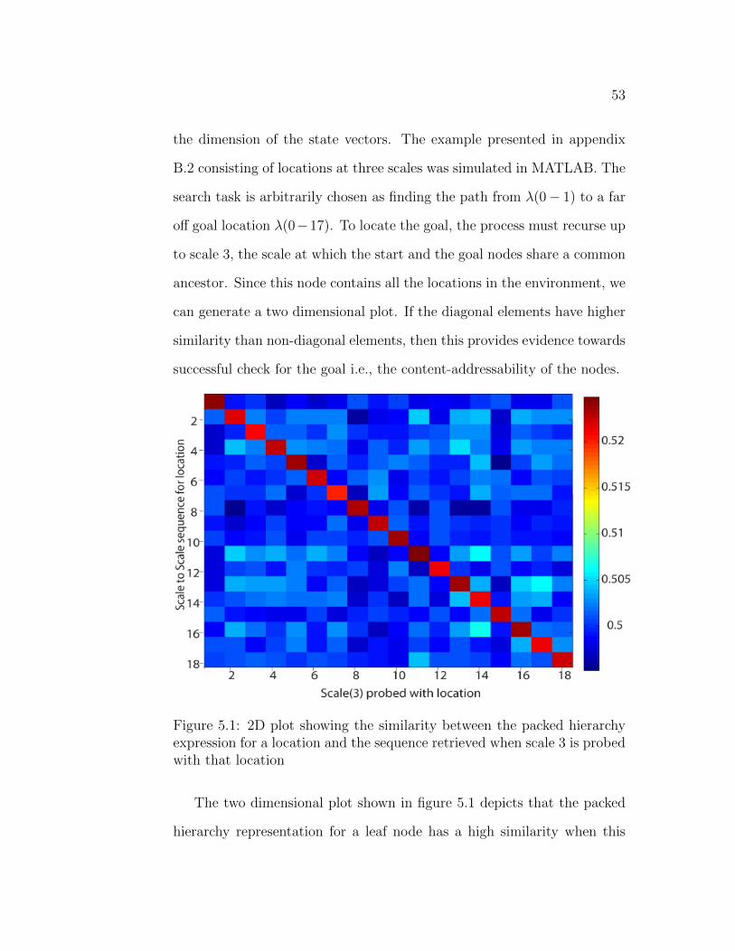
5.1 2D plot showing the similarity between the packed hierarchy

expression for a location and the sequence retrieved when

scale 3 is probed with that location . . . . . . . . . . . . . 53

5.2 Relationship of Accuracy and Confidence values with the

number of locations . . . . . . . . . . . . . . . . . . . . . . 54

5.3 Extremely sparse, hard-coded vectors . . . . . . . . . . . . 58

5.4 a) Vectors with 30 percent sparsity b) Doubly randomized

vectors with sparsity between 70− 90% . . . . . . . . . . . 60

5.5 Hopfield Net: The output of the network is recursively fed

back as input till the network stabilizes . . . . . . . . . . . 62

7

5.6 Hopfield Net: The left hand and right hand figures depict

the training samples and the output respectively. The red

and blue regions signify an activation value of 1 and 0 re-

spectively for that unit. The network was trained on 50

orthogonal patterns each represented along one column of

the two dimensional plot. It successfully retrieved the stored

patterns. . . . . . . . . . . . . . . . . . . . . . . . . . . . . 63

6.1 Virtual 3D environment explored by the participants. . . . 66

6.2 The inside of a building within the virtual world. Land-

marks such as the red star and the blue circle facilitate the

creation of a spatial map . . . . . . . . . . . . . . . . . . . 67

6.3 From left to right: Map of Building 1, 2 and the neigh-

borhood. The first two are locations at scale 0 while the

neighborhood is at scale 1 . . . . . . . . . . . . . . . . . . 68

6.4 Grand Average ERP Waveforms: These waveforms were

created by averaging together the averaged waveforms of

the individual subjects across the different trials. These

recordings are from the cortical areas above the occipital

lobe, the visual processing region. . . . . . . . . . . . . . . 72

6.5 The Paired Samples T test is used to compare the conditions

pair-wise. Significant differences were found for Pair 1 and

Pair 7 (p < 0.05). Refer to table 6.1 for the experimental

conditions corresponding to the condition numbers. . . . . 73

8

B.1 Spatial hierarchy depicted in graph-form. In this example,

there are 18 locations at the most refined scale, which are

grouped into 6 locations at scale 1, 2 locations at scale 2

and 1 location at scale 3 . . . . . . . . . . . . . . . . . . . 79

B.2 Spatial hierarchy depicted in graph-form. In this example,

there are 18 locations at the most refined scale, which are

grouped into 6 locations at scale 1, 2 locations at scale 2

and 1 location at scale 3 . . . . . . . . . . . . . . . . . . . 86

B.3 Relationship of Accuracy and Confidence values to Dimen-

sionality . . . . . . . . . . . . . . . . . . . . . . . . . . . . 92

List of Tables

3.1 Table summarizing the description, domain and range for

various functions . . . . . . . . . . . . . . . . . . . . . . . 32

6.1 The condition numbers allotted to the 6 experimental condi-

tions. Each of the three maps could be identified as “most

relevant” or “not relevant” by the participant. However,

their response is not taken into account in the analysis pre-

sented here. . . . . . . . . . . . . . . . . . . . . . . . . . . 69

6.2 The three maps and the two options (relevant or not rele-

vant) create a total of 6 conditions . . . . . . . . . . . . . 69

9

Chapter 1

Introduction

Locomotion is one of the essential features that distinguish animals from

plants. Birds and fish travel several thousand kilometers, undertaking

the journeys to their breeding or feeding grounds with incredible accuracy

and economy. Rodents in the wilderness regularly find their way around

hundreds and thousands of locations in their natural habitat. To orient

themselves and search through the space, animals may use multiple, multi-

modal cues such as magnetic, visual (e.g. stars, sun, landmarks), olfactory,

auditory, electrical or tactile cues [Dolins and Mitchell, 2010]. These con-

stitute the “compass” of the organism. Research into the sensory process-

ing mechanisms has produced daunting amounts of anatomical data. The

capacity to remember and learn allows spatial knowledge to be condensed

into an internal representation. It has been more than sixty years since Ed-

ward Tolman provided experimental evidence to demonstrate the existence

of a cognitive map [Tolman, 1948]. The compass and the map, both play

a crucial role in spatial navigation. While the ‘compass is relatively well

10

11

understood, the spatial map and its properties remain elusive. We don’t

even have a good framework for understanding how spatial information

is organized and used in pathfinding. Fundamental questions regarding

the cognitive map still remain unanswered. How are locations represented

in the brain? What are the functional and computational properties of

the map? How are the locations acquired, composed, stored, recalled and

decoded? While our scientific techniques have advanced tremendously, we

have a long a way to go before we can uncover the neural correlates of the

spatial map.

1.1 Discussion of Spatial Knowledge

Models of spatial knowledge must address two fundamental concepts:

• Spatial Representation which pertains to how and what kind of

information is stored in the spatial map.

• Spatial Reasoning which deals with the process or algorithm used

to peruse the map and search for paths between specific locations.

Even before the existence of a cognitive map was proven, Henri Berg-

son, an influential French philosopher who specialized in intuition, held

the belief that “whereas space is continuous, our model of it is created by

artificially isolating, abstracting, and creating fixed states of consciousness

and integrating them into a simultaneity.”[Reese and Lipsitt, 1975]

Perhaps when Bergson talked about “integrating them into a simul-

taneity”, he was referring to a hierarchical framework. Consider this: our

12

mental conception of a city is based on all the locations we have visited.

Somehow the lower level spatial entities such as buildings, parks, roads

etc. are amalgamated to give rise to the notion of a city. As we ascend

the hierarchy, higher-level, more abstract concepts are created.

We will be working under the premise that consciousness arises from

the activity of neurons. I take the liberty of interpreting his notion of

”fixed states of consciousness”; he was surely referring to distributed rep-

resentations. If the representation of spatial locations had a one-to-one

mapping with neurons, the spatial map would be extremely vulnerable

to damage. In computational neuroscience, concepts are represented by

a network of neurons across their pattern of firing, known as distributed

representations.

1.2 Related Work

Space has been scrutinized through a multitude of lenses and for varying

purposes. Computational models for representing spatial knowledge have

been developed for various purposes such as mobile robot technology, ge-

ographical computation and Vehicle Navigation Systems. Computational

vision systems may combine spatial and temporal data to analyze the dy-

namics of visual scenes ([Cohn et al., 2002], [Rohrbein et al., 2003]). In bi-

ological models of spatial cognition, spatial quantities may be represented

by the means of path integration - the distance and direction from a start-

ing point are kept in memory while traversing a two or three dimensional

environment [Etienne and Jeffery, 2004].

13

There have been numerous experimental studies exploring the path

finding ability of rats in linear tracks, in different types of mazes such as

the T-maze, alley mazes as well as 2D environments such as the Morris

water maze. These have demonstrated the existence of a cognitive map

[O’Keefe and Nadel, 1978]. The mechanisms of path finding and naviga-

tion is a classic problem that is still being actively pursued. Kubie et

al. propose a model based on vector arithmetic [Kubie and Fenton, 2008];

however, it remains to be seen whether vector addition is carried out in the

neuronal populations. Hopfield’s model based on hippocampal place cells

is not free from sequential search; at a decision point, the rat randomly

chooses a path [Hopfield, 2010]. This leads to rapid decrease in perfor-

mance with increase in the size of the environment. Hierarchical search

provides an escape from the sloth and high costs of sequential search.

Space, while continuous, can be readily molded into a hierarchical struc-

ture. Many studies have discovered the existence of hierarchies in the

saliency of spatio-temporal information in human and non human pri-

mates [Dolins and Mitchell, 2010]. The Hierarchical Path View Model of

Pathfinding for Intelligent Transportation Systems creates a hierarchical

description of the geographical region based on road type classification

[Huang et al., 1997]. The model presented here builds upon these ideas

and proposes a novel hierarchical model of spatial reasoning. The spatial

representation scheme used is that of distributed representations which

have been previously employed in computational modeling of the seman-

tics of language (in extracting analogical similarities, etc.) [Plate, 2000].

These are examined in greater detail in section 2.2.1.

14

Many Event Related Potential (ERP) studies have explored spatial

navigation and the role of spatial attention in visual processing. Matthew

Mollison examined the elicited electrical potentials during recognition of

landmarks near target vs. non-target locations in a 3D virtual spatial

navigation task [Mollison, 2005]. The event related potentials showed a

significance difference in the P300 component in the parieto-occipital re-

gions. This experiment shows that “target” vs “non-target” landmarks

can attain conceptual significance in the spatial map.

Other experiments have demonstrated that it is possible to prime an

individual towards certain spatial locations through sustained attention.

Awh et al. showed that when specific locations were held in the working

memory, attention was directed towards these locations [Awh et al., 1998].

Visual processing of stimuli appearing at that location is enhanced com-

pared to that of stimuli appearing at other locations. Experiments in-

volving non-spatial tasks did not produce any such attentional orienta-

tion supporting the association between spatial working memory and se-

lective attention. Another study demonstrated that if the shifts of at-

tention to memorized locations is interrupted, memory accuracy declines

[Awh and Jonides, 2001]. Further, they found voltage fluctuations during

the earliest stages of visual processing. This suggests that expectancy re-

garding the location on the screen affects its perception at a very early

stage in visual processing. These studies support the idea that the brain

uses memories to form predictions about what it expects to experience

before [one] experiences it. [Hawkins and Blakeslee, 2004].

15

1.3 Contributions

Holographic Reduced Representations (HRRs) provide a way of encod-

ing a complex structures such as a hierarchy within the framework of

distributed representations. I present two models of hierarchical spatial

reasoning based on different types of HRRs: Plate’s real-valued HRR and

Kanerva’s Binary HRR [Plate, 1991, Kanerva, 1997]. Various operations

in the HRR framework result in noisy vectors which are cleaned up in an

autoassociative memory; during the path-finding process, locations are re-

trieved using autoassociative recall. To test the hypothesis of hierarchical

spatial reasoning, I designed an ERP experiment that introduces atten-

tional bias towards a particular level in the hierarchy through the use of a

pathfinding task.

1.4 Structure of Thesis

The theoretical groundwork introduced in this chapter will be examined

in greater detail in chapter 2. It presents the foundational ideas in connec-

tionism and neuroscience that form the basis of the pathfinding framework

and process presented in chapter 3. The model presented in this chapter

uses binary representations. An extension to the continuous domain using

Plate’s convolutional algebra is presented in chapter 4. Chapter 5 presents

the results obtained from running different tests on the framework and

process. Chapter 6 describes an ERP experiment designed to test the

paradigm of hierarchical spatial reasoning at a high level.

Chapter 2

Background & Preliminaries

The model presented in this thesis is inspired by artificial intelligence and

neuroscience. This chapter presents some foundational ideas on knowledge

representation, hierarchical reasoning in the brain and connectionism. Sec-

tion 2.2 provides the preliminaries that are crucial to understanding the

models presented in subsequent chapters.

2.1 Background

The spatial map consolidates and depicts spatial knowledge, including the

paths, the relationship between different entities, etc. The problem of

spatial representation and spatial reasoning has been addressed by com-

puter science and neuroscience in various ways. This section presents a

general overview of some of these approaches with special emphasis on a

hierarchical framework.

16

17

2.1.1 Neuroscience background

The divide and conquer strategy used in hierarchical algorithms is not con-

fined to computer science. There is evidence that humans abstract space

into multiple levels [Car and Frank, 1994]. In fact, a diverse range of neu-

ral modalities such as visual perception, language and cognition operate

within a hierarchical layout. This topology is found in the organization of

the cortex - a sheet of neural tissue that forms the outermost layer of the

mammalian brain. This region developed later in the evolutionary pro-

cess than sensory processing regions. It plays an important role in many

higher-level functions such as attention, language and cognition. Converg-

ing evidence from many sources indicate that the topography of the cortex

is extensively hierarchical; the majority of the human cortex contains asso-

ciation areas where converging streams of information from many different

systems are integrated [Felleman and Van Essen, 1991, Essen and Maunsell, 1983].

For instance, lower-level information about the colors, shapes, textures etc.

is combined in the cortex such that one cell may fire specifically in response

to faces. The spatial and temporal patterns are integrated to form more

abstract, higher level, stable representations as we ascend the levels of the

cortical hierarchy (see figure 2.1.1).

Hierarchical Temporal Memory(HTM) is a promising model of infor-

mation processing in the neocortex within a mathematical and algorith-

mic framework. “Information flows up and down the sensory hierarchies

to form predictions and create a unified sensory experience. This new

hierarchical description [HTM] helps us understand the process of creat-

18

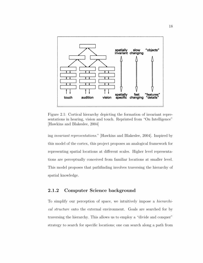
Figure 2.1: Cortical hierarchy depicting the formation of invariant repre-sentations in hearing, vision and touch. Reprinted from “On Intelligence”[Hawkins and Blakeslee, 2004]

ing invariant representations.” [Hawkins and Blakeslee, 2004]. Inspired by

this model of the cortex, this project proposes an analogical framework for

representing spatial locations at different scales. Higher level representa-

tions are perceptually conceived from familiar locations at smaller level.

This model proposes that pathfinding involves traversing the hierarchy of

spatial knowledge.

2.1.2 Computer Science background

To simplify our perception of space, we intuitively impose a hierarchi-

cal structure onto the external environment. Goals are searched for by

traversing the hierarchy. This allows us to employ a “divide and conquer”

strategy to search for specific locations; one can search along a path from

19

top to bottom, excluding large areas of the problem space. Such models

can improve upon other strategies such as precomputing shortest paths or

exhaustive search, which tend to have high storage costs and worse case

complexity.

As mentioned in section 1.2, increasing computational cost with in-

crease in environment size is one of the major drawbacks of models based

on sequential or random search. Hierarchical search helps overcome this

shortcoming. Such models are traditionally represented in localist frame-

work and the number of localist elements required to represent a com-

plex recursive structure becomes prohibitive because of exponential growth

[Rachkovskij, 2001]. Moreover, it involves meaningless pointer following to

retrieve the constituents at the lowest hierarchical level. This increase in

the cognitive load of the spatial representation becomes highly problematic

with increase in the size of the environment.

2.1.3 Connectionism

The goal of this project is to understand the neural basis of spatial cog-

nition in the brain. We approach this issue from the perspective of con-

nectionism - the study of mental phenomena as emergent processes of a

network of interconnected units. It derives inspiration from many fields

such as artificial intelligence, neuroscience, cognitive science, philosophy

of mind, etc. Connectionist models of information processing in the brain

are based on a few simple, fundamental principles [McLeod et al., 1998]

1. The basic computational operation in the brain involves one neuron

20

passing information related to the sum of the signals reaching it to

other neurons.

2. Learning changes the strength of the connections between neurons

and thus the influence one has on another.

3. Cognitive processes involve the basic computation being performed

in parallel by a large number of neurons.

4. Information, whether about an incoming signal or representing the

network’s memory of past events, is distributed across many neurons

and many connections.

Connectionist models have many useful features such as graceful degra-

dation, automatic generalization, fault tolerance, etc.

Parallel, Distributed processing in Cognitive Models

Traditional models of cognitive processing as well as those of pathfind-

ing assume that information is represented in a localist fashion. In other

words, a concept in these models is stored at individual, independent loca-

tions. For instance, to implement a breadth first search, each node in the

graph may represent a particular location in the environment with edges

signifying the distance between these locations. On the other hand, repre-

sentation is distributed in connectionist models. This may seem counter-

intuitive to our notion of data storage, even storage in a general sense.

Consider this: on an average, thousands of neurons die everyday causing

random loss of information. Moreover, there is a certain amount of noise

21

and stochasticity associated with neural firing. The brain has found a so-

lution to unpredictability by performing parallel computations on concepts

that are distributed over many neurons.

Distributed Representations

As previously mentioned, distributed representations are high-dimensional

vectors that are used to represent concepts. They have many advantages

such as:

• Automatic Generalization: Locations that are similar will have

similar patterns of activation; they do not need to be explicitly repre-

sented as similar; similar activation patterns produce similar results.

This is biologically realistic since signals received in the brain which

are hardly ever identical, are nevertheless identified as specific ob-

jects, places, people, scenes, etc [Kanerva, 1993].

• Representational efficiency: Distributed representations can pro-

vide a more efficient code than localist representations. A localist

representation using n neurons can represent just n different entities.

A distributed representation using n binary neurons can represent up

to 2n different entities (using all possible patterns of zeros and ones)

[Plate, 2002].

• Soft Capacity Limits and Graceful Degradation: distributed

representations typically have soft limits on how many concepts can

be represented simultaneously before interference becomes a serious

22

problem. The accuracy of goal retrieval degrades gradually with in-

crease in the size of environment or damage to the neural structures.

In the 90s, connectionism faced a major roadblock: it was missing a tech-

nique for representing more sophisticated structures such as trees within

a distributed framework. Hinton introduced the notion of a reduced de-

scription as a way of encoding complex, conceptual structure in a distributed

framework [Hinton, 1990]. Holographic Reduced Representations (HRR)

capture the spirit of these reduced representations[Plate, 2003]. The ex-

traordinary feature of HRRs is that they allow the representation of a

concept across the same number of units as each of the constituents, thus

avoiding the problem of expanding dimensionality. HRRs provide a way

to combine two vectors to make a memory trace that is represented across

the same number of bits. Even more remarkably, the memory trace can be

used along with one of the original vectors to retrieve the other. (Hence

the term holographic which refers to the technique of storing and recon-

structing the light scattered from an object after the object is no longer

present). With its many attractive qualities, HRRs provide an ideal tool

for constructing a model for hierarchical spatial reasoning in a two dimen-

sional environment. This work presents a novel application of HRR in

hierarchical pathfinding.

2.2 Preliminaries

In the last section, we learnt that a connectionist model represents con-

cepts in a distributed fashion. In subsection 2.2.1, these representations

23

and their properties are examined in greater detail. This will be rele-

vant to understanding the Pathfinding Framework and Process presented

in Chapter 3. Subsection 2.2.2 introduces the concept of an autoassocia-

tive memory that supports parallel computation in a biologically realistic

fashion.

2.2.1 Distributed Representations

Distributed representations use high-dimensional vector spaces to repre-

sent the elements of the model, i.e. locations in the environment. Dis-

tributed representations have two main properties:

• Each concept (e.g., an entity, token, or value) is represented by more

than more neuron (i.e., by a pattern of neural activity in which more

than one neuron is active.)

• Each neuron participates in the representation of more than one

concept.

In this model, the neural codes or patterns of activity corresponding to

locations in the environment are represented as fixed, high-dimensional,

binary vectors. Similarity of two neural patterns can be computed in dif-

ferent ways depending on the framework. When using real-valued vectors,

similarity is the dot product followed by thresholding or normalization. For

binary vectors, similarity is defined as the number of corresponding, iden-

tical bits in the two vectors. Two operations are used to form associations

within this framework: binding and merge operation, both of which retain

the dimensionality of the vectors on which they operate.

24

Binding Operation

The binding operation on two vectors combines them into a third vector

which is not significantly similar to either one of its constituents. The

resulting vector known as trace can be used with one of the constituting

vectors to retrieve the other vector. Binding is a flexible operator with

many useful properties:

• Commutativity: A©B = B© A

• Associativity: (A©B)© C = A© (B© C)

• xor has the unique property of self-inverse: A© B © B = A and

B©B© A = A

The binding operator for binary representations is the exclusive-or (xor)

operator (denoted by ⊗) - a logical operator that results in true iff exactly

one of the operands is true. In this case the decoding is perfect; the re-

trieved vector is identical to the original. For real-valued distributed rep-

resentations such as the ones in Plate’s convolutional algebra, the binding

operator is the convolution operator. [Plate, 1995]

Merge Operation ‘+’

This is an important feature of distributed representations; the superpo-

sition or merge operation between two or more vectors generates a vector

that is similar to each of its constituents. There is no “unmerge” op-

eration that allows decoding from superposition. Since the vectors are

independently and uniformly distributed, high-dimensional vectors, there

25

is a minuscule probability for two random vectors to have higher than sig-

nificant similarity by pure chance. The binding operation is distributive

across merge: Distributivity: A© (B + C) = (A©B) + (A© C)

The merge operation for binary vectors is known as thresholding - each

bit of the result vector is 0 or 1 depending on which appears in that position

most often among all the constituting vectors; ties are broken at random

with probability 0.5. In this thesis, the merge operation is denoted by ‘+’,

not to be confused by the addition operator.

2.2.2 Autoassociative Memory

The intuition behind an autoassociative memory is the simple idea that

“the distances between concepts in our mind correspond to distances be-

tween points in a high-dimensional space [Kanerva, 1993]. An autoasso-

ciative memory stores different patterns of activation across the same set

of connections. It is able to perform pattern-completion and thus is an

ideal candidate for a computational model of recall. The auto-associative

memory takes a noisy vector as input and outputs a specified number of

vectors with the highest similarity scores (or indicates that the input is

not significantly similar to any of the stored vectors). It is used to clean

up the noisy vectors that result from various encoding and decoding op-

erations. This is similar to a standard item memory which retrieves the

best-matching vector when cued with a noisy vector, or retrieves noth-

ing if the best match is no better than what results from random chance

[Kanerva, 1998]. In our implementation the auto-associative memory can

26

return more than one item if each gives a high similarity and the similarity

values are very close to each other (within 1%). These memories give the

system the capacity for recall along with recognition.

2.2.3 Hierarchical Spatial Reasoning

As mentioned in section 2.1.2, this model imposes a hierarchical framework

on the environment. Let the natural habitat contain salient locations sepa-

rated by empty stretches that are not explicitly represented in the cognitive

map. Information about the discrete, salient locations is acquired from the

environment through extended exploration and is consolidated within a hi-

erarchical framework. This section introduces terminology pertaining to

this tree data structure that will support the pathfinding process. Leaf

nodes or leaves are the locations in the environment at the smallest scale.

All other nodes in the tree, referred to as internal nodes (I), are composed

of nodes at smaller scales (See figure 2.2). For instance, if individual rooms

inside a building were to be leaf nodes, the building, the neighborhood,

and other locations at higher scales would be represented as internal nodes.

Every leaf node has a parent, i.e., the node it belongs to at the next

higher scale. The depth of a tree is the length of a path from the root to the

node. The root node at the topmost level has depth 0. In our model, we

will assume that all the leaves are at the same depth. Every internal node

has at least one child. The height of the tree is the depth of a leaf node.

The scale of a given node is defined as the height − depth. This gives us

a numbering system where locations at more refined levels have a smaller

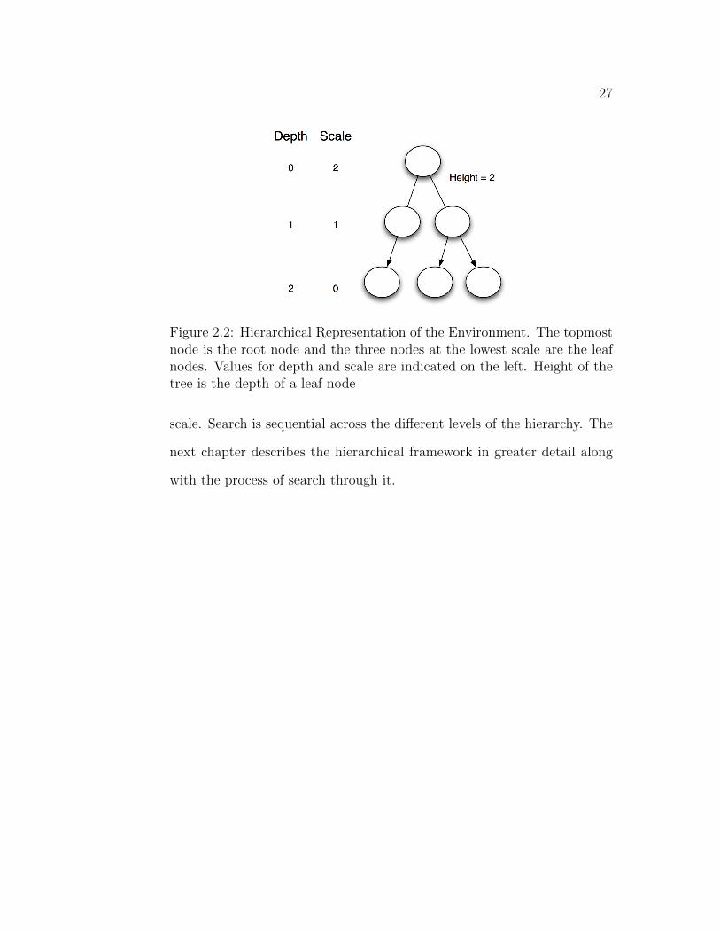
27

Figure 2.2: Hierarchical Representation of the Environment. The topmostnode is the root node and the three nodes at the lowest scale are the leafnodes. Values for depth and scale are indicated on the left. Height of thetree is the depth of a leaf node

scale. Search is sequential across the different levels of the hierarchy. The

next chapter describes the hierarchical framework in greater detail along

with the process of search through it.

Chapter 3

Pathfinding Framework and

Process

“All truly great thoughts are conceived while walking” - Nietzsche

Chapter 2 introduced Holographic Reduced Representations as a tech-

nique of encoding complex, compositional structure. In this chapter, these

are used as building blocks to create a hierarchical representation of the

environment i.e., the framework. The framework consists of an autoas-

sociative memory that stores different compositional vectors. They con-

ceptually represent the associations formed between various locations in

the environment. During the pathfinding process, locations are retrieved

using autoassociative recall. Section 3.1 describes the framework which

involves the recursive generation of state vectors for locations at higher

scales. Section 3.2 describes the process of searching for a path from a

start location to a goal location within this hierarchical framework. The

28

29

autoassociative memories that were populated in Section 3.1 are queried

at many stages of the pathfinding process.

3.1 Pathfinding Framework

This model works under the assumption of a fully-explored environment.

In other words, the leaf nodes of the tree described in subsection 2.2.3 are

given as input to the model. These distinct, discrete locations are rep-

resented using randomly generated, high-dimensional, binary distributed

state vectors (the extension to the continuous domain is presented in Chap-

ter 4.) State vectors corresponding to nodes at higher scales of the spatial

hierarchy are recursively generated using the nodes at lower scales. These

state vectors are stored in the autoassociative memory, in some cases after

further composition. This section describes the ”pre-processing” steps or

the compositional rules of the process required to generate the hierarchy

(shown in figure 3.1).

Let us introduce set notation to formalize the distributed framework

associated with the spatial hierarchy. Let T=(V,E) denote the tree repre-

sentation of the spatial environment. V is the set of all nodes in the tree

and E (edges) conceptually encode the hierarchical ordering; they are not

explicitly represented but are useful in hierarchical composition. Elements

of the set V are one of two types: leaf nodes and internal nodes (previously

introduced). If L is the set of leaf nodes and I is the set of internal nodes,

the equivalent description in set notation is given by: T(V,E) = L ∪ I.

All nodes are represented as state vectors with d individual units (the di-

30

Figure 3.1: A sample hierarchical framework depicted in graphical form.Each location at higher scale is composed of the constituting locationsat lower scales. Indexes are indicated next to the scale number. Note:The edges do not encode any feature of the spatial environment such asdistances etc; they are merely a conceptual aid and not pointers as typicallyconceived in computer science. This works to our advantage in designinga recursive compositional rule.

mensionality d is usually between 1000-10,000). Each unit can be active

(’1’) or inhibited (’0’). The leaf nodes referred to as ψ are generated ran-

domly such that the probability of activation of each unit is 0.5.

ψ(psi) : L→ {0, 1}d

λ(lambda) : V → {0, 1}d

Section 3.1.1 presents the compositional rules for the recursive generation

of locations.

3.1.1 Hierarchical Composition of locations

Higher-scale locations are recursively composed of those at smaller scales.

This is based on the intuition that the state vectors for locations at higher

scales emerge from exploration of sub-regions and are systematically re-

31

Figure 3.2: Locations at scale i are merged together to obtain the mergedsequence µ(i+ 1, p). This vector is bound with a key κ(i+ 1, p) to obtainthe location at scale i+1, λ(i+ 1, p)

lated to them. As a reminder, the binding operation denoted by ⊗ is the

exclusive-or operation. It doubles up as the decoding operator. Similarity

between two binary vectors is computed as 1− Hd

where H is the Hamming

Distance and d is the dimensionality.

Every internal node v ∈ I is associated with a key vector and a merged

vector denoted by κ(n− i) and µ(n− i) respectively, where n is the scale

and i is the index of that location. A location at scale n (where n>0) is

constructed from a location at scale n-1 in two steps:

1. The constituting scale n− 1 vectors are merged or superimposed to

obtain the merged vector . The merged expressions, defined for all

internal nodes, are obtained as follows:

∀v ∈ I, µ(v) =∑

u∈children(v)

u

2. The vector for scale n is then computed by binding the merged vector

with a unique key κ(v) for that location: λ(n−i) = κ(n−i)⊗µ(n−i).

The spatial locations are defined as:

32

Function Domain and Range Intuitive Associationψ (psi) L→ {0, 1}d Leaf Nodesµ (mu) I → {0, 1}d Merged Vectorκ (kappa) I → {0, 1}d Keysλ (lambda) V → {0, 1}d Spatial Locations (State Vectors)π (pi) L→ {0, 1}d Packed Hierarchy

Table 3.1: Table summarizing the description, domain and range for vari-ous functions

∀v ∈ V, λ(v) =

ψ(v) if v ∈ L

κ(v)⊗ µ(v) if v ∈ I

Holographic Reduced Representations allow us to represent locations

from the smallest to the largest scale using the same number of units. The

nodes are systematically related to each other such that information about

their constituents can be gathered without expansion of the nodes into

their children (see section 3.2.1). Hence, not only is the dimensionality

preserved, the framework design proposed here ensures that the nodes

are content addressable. This provides an ideal setup for the hierarchical

pathfinding process presented in section 3.2.

3.1.2 Auto-associative Memory

In this path finding model, there are two main auto-associative memories

and a supplementary memory.

1. The Location memory stores all the locations at different scales such

as λ(0−1), λ(0−2), λ(1−1), λ(2−1), . . . , the keys κ(0−1), κ(1−2),

. . . This memory is queried to retrieve the location corresponding to

33

Figure 3.3: The Location memory stores all the state vectors and theirassociated keys. It stores as many state vectors as size(V) and as manykeys as size(I)

the next scale, when the goal is not found at the current scale.

2. The packed hierarchy memory consists of associations between the

location keys across all the nodes from the top to the bottom of the

hierarchy (see figure 1). Before we arrive at a description of these

vectors, let us recursively define set Anc(v,i) as the first i ancestors

of node v:

Anc(v, i) =

parent(v) if i = 1

parent(v) ∪ Anc(parent(v), i− 1) if i ≥ 1

Let N be the set of all the parents of the leaf nodes. The vectors

that populate the packed hierarchy memory are computed as:

∀v ∈ N, π(v) =

height(T )∑i=1

v ⊗∏

κ(a),∀a ∈ Anc(v, i)

This memory is queried to retrieve the location at the next higher

scale as well as to check whether the goal is present at a given loca-

tion.

3. The supplementary memory stores expressions obtained from su-

34

Figure 3.4: The different nodes along one branch of the hierarchy, from topto bottom, are packed into a sequence and stored in the packed hierarchymemory. The shaded path pertains to the vector: κ(1 − 5) + κ(1 − 5) ⊗κ(2 − 2) + κ(1 − 5) ⊗ κ(2 − 2) ⊗ κ(3 − 1) The number of such vectors isgiven by the size of set N, the set of all parents of the leaf nodes

perposing the key with the corresponding merged vector such as

κ(0−1) +µ(0−1), etc. This memory is queried to retrieve the state

vectors corresponding to the a set of keys. There are size(I) vectors

of this type in the memory.

Note: It is assumed that locations within a grouping are interconnected

i.e., there exists a path connecting every pair of nodes that share a parent.

3.2 Processes

Now that we have a representation of the spatial hierarchy, let us see how

it is useful in finding the path from one location to another. Pathfinding

35

Figure 3.5: The Supplementary memory stores superposed expressionswith the keys and the merged vector

happens sequentially from top to bottom, across the nodes at different

scales of the hierarchy. There are various sub-operations involved as shown

in the figure below. As we ascend the scales, the nodes preserve their

dimensionality; however they become conceptually heavier since more state

vectors are being packed. Thus, there is a tradeoff between efficiency of

hierarchical search and increase in the noise of the system.

To find a path from the start location to the goal location in this

environment, locations at higher scales are searched until a location is

found that contains both the start and goal locations. Once this location

has been found, the corresponding locations at smaller scales are retrieved

so as to find the path leading to the goal.

In the illustration above (Figure 3.6), let us look for the path from a

start location in λ(1−1) to a goal location in λ(1−5). One searches across

the hierarchy of scales upto λ(3− 1) and is able to retrieve the path as a

subset of the nodes in the tree:

(start) → λ(2− 1)→ λ(3− 1)→ λ(2− 2)→ λ(1− 5)→ goal.

36

Figure 3.6: Example tree depicting nodes (discrete locations) at differentscales. Pathfinding is hierarchical across the different scales.

This process and the associated sub-processes are summarized in the pseudo

code below:

function(current, goal)

while start! = goal (Use the goal location to test this)

Retrieve location at next scale

current = next

Use Location memory to check whether start is the goal

end while

if current==goal

Generate a query using the current goal

for i= 2 to scale-1

Probe location memory with the query to retrieve

scale i node using scale i-1 node

Generate new query by combining scale-i node with

previous query

37

end for

end if

else: goal not found

This process is summarized in the high-level description of the search

process shown in figure 3.7. Each of the three operations are explained

in subsequent sections: checking for the goal (3.2.1), moving up a scale

(3.2.2) and retrieving all the ancestors of the goal node (3.2.3).

Figure 3.7: Flow chart depicting the various stages of the pathfindingprocess

3.2.1 Checking for the Goal

Searching for the goal g at any given location X is accomplished by query-

ing the packed hierarchy memory with g ⊗ X. This is also called probing

X with g [Kanerva, 1997]. This expression will retrieve a vector with a

38

Figure 3.8: Flow chart depicting the various steps involved in checking forthe goal

high similarity value in the packed hierarchy memory iff X contains the

goal. This feature has been designed into the framework to ensure that

the nodes are content-addressable. Else, hierarchical search would not be

possible. A more comprehensive look at this property reveals two aspects

that make it possible:

• Algorithm Design: The location expressions are composed of merged

vectors and their associated location keys. The probe operation “un-

locks” a node only if it contains the goal node.

• Self-inverse property of xor: At a more fundamental level, the

working of the probe operation relies on the fact that xor can be

used as the binding and unbinding operation.

39

3.2.2 Retrieving the next Scale

Figure 3.9: Flow chart depicting the various steps involved in retrievingthe parent node

The current location at scale m when combined with all the previously

encountered locations at smaller scales can be used to retrieve the location

at the next higher scale. This is described in a pseudo code form below

followed by a more detailed description:

• The packed hierarchy memory is queried with current location at the

smallest scale (scale 0) which will return a high similarity with an

expression of the form:

40

StoSx = λ(0−x)+λ(0−x)⊗λ(1−y)+λ(0−x)⊗λ(1−y)⊗λ(2−z)+. . .

Note: This first step is performed only once - when the current

location is at scale 0.

• Let Y be the expression obtained from binding all the locations at

the different scales from the current location at scale 0 to scale m.

To retrieve the location at scale m+1 the location memory is queried

with: Y ⊗ StoSx.

These steps are summarized in the flow chart 3.9.

Note: For m>0, a disambiguation step is required since locations at

scale m+1 and scale m are returned. The returned location is either the

location at the next scale (desired) or the location at the current scale;

therefore comparison with the current scale location is sufficient to obtain

the location at the next scale.

3.2.3 Retrieving the Path

Once the goal has been found, all the ancestors to the goal node can be

retrieved by recursive querying of the memory. Let goalExp be the packed

hierarchy expression returned by the memory. The path is retrieved in the

following steps:

• The Location memory is queried with the packed hierarchy vector P.

Let the retrieved vector be X. This would be the parent of the goal.

• Generate a query X ⊗ P . Use this to retrieve the parent of X from

the location memory; this is the new X.

41

Figure 3.10: Flow chart depicting the various stages in retrieving the pathonce the goal has been found. The memory is queried recursively for thechildren nodes associated with the node at which the goal was found

42

• Perform the previous step till all the ancestors for the goal have been

retrieved.

• The final step in retrieving the path involves finding the merged

vectors corresponding to the keys retrieved in the previous step. The

supplementary memory is queried with the key κ to retrieve vector

PH.

• The location memory is queried with κ ⊗ PH to retrieve the corre-

sponding merged vector µ.

In the illustration above, the goal is found at scale 3, the smallest

scale containing both the goal and the start location. Let the expression

returned from the memory be called PH17. Using the goal key κ(0 − 17)

and PH17, we can successively retrieve the locations keys at the different

scales along the path to the goal. This is an expansion operation with

scale keys.

κ(0− 17) = ⊗PH17 = κ(0− 17)⊗ (κ(0− 17)⊗ κ(1− 5) + κ(0− 17)⊗

κ(1− 5)⊗ κ(2− 2) + κ(0− 17)⊗ κ(1− 5)⊗ κ(2− 2)⊗ κ(3− 1))

= (κ(1− 5) + κ(1− 5)⊗ κ(2− 2) + κ(1− 5)⊗ κ(2− 2)⊗ κ(3− 1))

∼ κ(1− 5)

Similarly κ(0− 17)⊗ κ(1− 5) can be used to retrieve the location at the

next higher scale λ(2− 2). If the goal was found at scale n, the expansion

operation involves n− 2 such steps are required to find the different scales

at which the goal is present and retrieve the path to the goal.

43

To retrieve the merged vectors for the keys, the location memory is

queried using the keys κ(1 − 5) and κ(2 − 2). This returns κ(1 − 5) +

κ(1− 5)⊗ µ(1− 5) and κ(2− 2) + κ(2− 1)⊗ µ(2− 2) respectively. These

expressions are bound to their respective keys and are used to query the

Location memory recursively returning: (0 + µ(1 − 5)) ∼ µ(1 − 5) and

(0+µ(2−2)) ∼ µ(2−2) Through this recursive sub-process, one retrieves

the representations at different scales for the path towards the goal:

µ(3− 1)→ µ(2− 1)→ µ(1− 5)

This path may be a novel route that was never traversed, which was re-

trieved based on the stored associations.

For a specific example of pathfinding see Appendix B.1.

3.3 Features of the Algorithm

This process exploits the property of the framework that each node in the

search tree is content-addressable to some extent. Direct accessibility to

nodes allows us to search across scales rather than sequentially across all

the locations. This avoids combinatorial explosion of costs in larger envi-

ronments. We have seen that the noise in the system increases with the

number of locations in the environment. One can overcome this drawback

and the subsequent loss in accuracy by breaking down the problem hier-

archically. Let the scale 1 node corresponding to the goal be known. The

problem is reduced to searching for the scale 1 node in the cognitive map

of the environment followed by searching for scale 0 node within the scale

1 node. Such a modification to the algorithm requires an additional set

44

of sequences to be stored in the packed hierarchy memory namely packed

hierarchy sequences with scale 1 nodes.

3.4 Analyzing the Process

In this section I present the computational cost involved in different pro-

cesses and sub-processes.

Let there be n locations in the environment each represented as a vector

of dimension d. The preprocessing storage requirements for the three types

of auto-associative memories are as follows:

1. The Location memory contains the representations for all the lo-

cations at various scales of the hierarchical spatial map. We know

that if there are n leaf nodes then the maximum number of nodes

in the tree is given by the number of nodes in a binary tree with n

leaf nodes. Hence, if there are n locations at the lowest level of the

hierarchy, then the total number of locations is:

20 + 21 + . . .+ 2logn =2logn+1 − 1

2− 1= 2(2logn)− 1 = 2n− 1

Hence, total storage space required S = (2n-1)d.

2. The secondary memory stores all the keys, values and expressions

combining the keys and values. Since all nodes in the tree are asso-

ciated with keys and values except the ones at the lowest level of the

hierarchy. Pursuing a line of analysis similar to the one above gives

45

us the total number of keys/values as:

20 + 21 + . . .+ 2logn−1 = 2logn − 1 = n− 1

Since there are three sets of expressions involving either keys, values

or both, the total space required S = 3 ∗ (n− 1) ∗ d

3. The packed hierarchy memory contains as many expressions as there

are locations, giving us a total storage requirement of (2 ∗ n− 1)d.

Now we analyze the performance of the algorithm with increase in the

size of the environment. The expression at the highest scale contains a

total of x∗ y ∗ z = n terms merged together. As we increase the number of

vectors that are packed into one sequence, the noise in the system increases

till checking for the goal no longer gives reliable results. Let K be the

number of terms in X = [A + B + ... + D(+R)]. To analyze the limit

on the size of the environment, we compute the limit for K for which the

probability that X and A are the same, α(X,A) is significantly different

from α(A,B) the probability that two random vectors A and B are the

same. α(X,A) = 1− delta(X,A) where δ(X,A) is the expected Hamming

distance between X and A, i.e. the probability that X and A differ. It is

given by

δ(X,A) =1

2− 1

2K

(K − 1K−12

)(3.1)

(For derivation of δ, see appendix A)

which is approximated as 0.5− 0.4√K − 0.44 [Kanerva, 1997]

The standard deviation of the binomial distribution for two random

46

vectors is given by σ =√

δ(1−δ)N

. For two random vectors of length N =

10, 000, δ = 0.5, σ = 0.005 is so small that δ(X,A) need not be far from

0.5 to be significantly different from it [Kanerva, 1997]. Sequences with

K > 177 are associated with an alpha value lower than 0.53 and for those

with K> 255 have an alpha value lower than 0.525. If a relatively fewer

runs are desirable, then we could assign an upper limit such as K= 200 as

the upper limit for α(X,A) to be reliably distinguishable from alpha for

two random vectors in a certain number of runs< 30.

Chapter 4

Extension to Continuous

Domain

“You have your way. I have my way. As for the right way, the correct

way, and the only way, it does not exist.” - F. Nietzsche

A second model of hierarchical spatial reasoning was developed. The

extension to continuous domain is realized using Plate’s Holographic Re-

duced Representations [Plate, 1991]. This representation scheme uses a

high-dimensional continuous space of real-valued vectors. To recap, the

similarity between two vectors is calculated as the normalized dot prod-

uct. The merge operation is carried out through bit-wise addition followed

by normalization. The Binding operator within this framework is the cir-

cular convolution operator shown in figure 4.1. This is a compressed outer

product with the unique property of preserving the dimensionality of the

resultant vector, a.k.a. the memory trace. Plate’s convolutional algebra

47

48

has the remarkable feature that it can decode the trace to retrieve one

of the original vectors that participated in the binding operation. The

involution of c, denoted by cT results in a vector d such that di = c−i,

where the subscripts are modulo-n. Involution operation functions as the

approximate inverse of convolution. Decoding is achieved by taking the

involution of one of the vectors used in encoding, and convolving it with

the memory trace.

Figure 4.1: Circular Convolution Represented as a compressed outer prod-uct for n= 3 [Plate, 1995]

4.1 Extension to Framework

As in the case of the binary framework, state vectors for higher level nodes

are recursively composed of those at smaller scales. The compositional

rules, however, are different for the locations as well as the vectors stored

in the auto-associative memory. One does not require keys or merged

vectors in this scheme. This is made possible by the design of the state

vectors using the auto-convolution operation i.e. convolution of a vector x

with itself - x~ x.

49

Once again, let T=(V,E) denote the tree representation of the spatial

environment where V is the set of all nodes in the tree and E (edges)

conceptually represents the hierarchical ordering. This set is sectioned

into a subset of leaf nodes L and internal nodes I. Each of the leaf nodes

is assigned a real-valued vector that has a mean at 0 and a variance of

1d

[Plate, 1995] (the dimensionality of the vector, d is typically assigned a

value of 2048).

4.1.1 Autoassocaitive Memories

As mentioned previously, the merge, also denoted as summation in the

equations below, is bit-wise addition followed by normalization. The cir-

cular convolution operation is also referred to as a product in this chapter;

since product and sum do not have any default meanings in the world

of distributed representations, this is reasonable. The continuous frame-

work presented here requires two types of sequences to be stored in the

auto-associative memory:

• The Location memory which contains all the locations. The internal

nodes are composed as follows:

∀v ∈ L, λ(v) =∑

u∈children(v)

v ~ v

• The packed hierarchy memory consists of associations between loca-

tions at different scales. For each leaf node, vectors in this memory

pack the complete hierarchy from top to bottom. Before defining the

compositional rule, let us define set Anc(v,i) as the first i ancestors

50

Figure 4.2: Flow chart depicting the process of composing state vectorsfrom nodes at smaller scales

of node v:

Anc(v, i) =

parent(v) if i = 1

parent(v) ∪ Anc(parent(v), i− 1) if i ≥ 1

The vectors that populate the packed hierarchy memory are com-

puted as:

∀v ∈ L, π(v) = v +

height(T )∑i=1

v ⊗∏

λ(a), ∀a ∈ Anc(v, i)

4.2 Extension to Process

From a high-level, the pathfinding process is essentially the same as in the

case of binary representations - search is hierarchical across the different

scales. However, the details of the operations have been modified for the

51

new framework presented in the previous section 4.1. The design of the

vectors is slated to ensure content-addressability of the nodes.

4.2.1 Checking for the Goal

Checking whether a particular node contains the goal requires the use

of the decoding (involution) operator introduced earlier. If the goal lo-

cation is represented by g and the location at the current scale is loc,

then loc contains g iff gT ~ loc returns an expression with high similarity

from the hierarchy packing memory. This confers the property of content-

addressability to the nodes of our tree, which in turn supports hierarchical

search.

4.2.2 Goal Retrieval

Let X be the expression returned from the auto-associative memory when

a node at scale n is probed with the goal g. Now, we can probe X with the

goal g to retrieve the goal location at scale n−1 from the packed hierarchy

memory, say f. Next we probe X with g ~ f to retrieve the goal at scale

n − 2 and so on. Thus we can recursively obtain goal locations at more

refined scales.

Chapter 5

Experiments and Results

“A casual stroll through the lunatic asylum shows that faith does not prove

anything.” -F. Nietzsche

The pathfinding process described in chapter 3 relies on being able

to directly query a node for any of its children. With increase in the

size of the environment, there is a decrease in the accuracy of identifying

whether a particular child node at a given scale is present. A proof of

correctness for the process is beyond the scope of this work. However,

the HRR framework was simulated in MATLAB. This chapter describes

results from experiments designed to test different aspects of the model.

5.1 Experiments on the Process

This section presents results on the the accuracy and confidence with which

the goal is retrieved and how it varies with the size of the environment and

52

53

the dimension of the state vectors. The example presented in appendix

B.2 consisting of locations at three scales was simulated in MATLAB. The

search task is arbitrarily chosen as finding the path from λ(0− 1) to a far

off goal location λ(0−17). To locate the goal, the process must recurse up

to scale 3, the scale at which the start and the goal nodes share a common

ancestor. Since this node contains all the locations in the environment, we

can generate a two dimensional plot. If the diagonal elements have higher

similarity than non-diagonal elements, then this provides evidence towards

successful check for the goal i.e., the content-addressability of the nodes.

Figure 5.1: 2D plot showing the similarity between the packed hierarchyexpression for a location and the sequence retrieved when scale 3 is probedwith that location

The two dimensional plot shown in figure 5.1 depicts that the packed

hierarchy representation for a leaf node has a high similarity when this

54

location is the goal location and low similarity otherwise. The sequences

in the packed hierarchy memory corresponding to every leaf node is rep-

resented along the x-axis. Hence, the x axis ranges up to the number of

leaf nodes in the environment. The y axis represents the query when the

aforementioned leaf node is assigned as the goal location. In other words,

the column y=k represents the query to the memory when k is the goal

and current location is λ(3− 1). The (i, j)th cell of the plot represents the

similarity between the packed hierarchy for that leaf node and the query

expression obtained using that leaf node as the goal. The similarity values

are color coded as depicted in the color bar on the right.

0 20 40 60 80 100 120 140

0.49

0.5

0.51

0.52

0.53

0.54

0.55

0.56

Number of locations

Sim

ilari

ty V

alu

e

Accuracy and Con!dence values for all locations

Accuracy

Con!dence

Figure 5.2: Relationship of Accuracy and Confidence values with the num-ber of locations

The accuracy value of a two-dimensional plot is defined as the average

55

of all the diagonal elements - it represents the average similarity between

the packed hierarchy sequence for a location and the sequence retrieved

when that location is assigned as the goal. The confidence value is defined

as the average of all the non-diagonal elements. It represents the average

similarity between the packed hierarchy sequence for a location and and

the sequence retrieved when any other locations are assigned as goals.

The next figure 5.2 is created using the accuracy and confidence values

computed for each two dimensional plot when the number of nodes in the

tree are varied. The size of the environment ranges from 3 to 138 individual

locations (leaf nodes) each represented as 5000-dimensional vectors. As

expected, the confidence values are near 0.5 showing that the similarity

of the query for non-corresponding nodes is as good as random. Since

the number of scales is kept constant across environments with increasing

size, greater number of locations are packed to obtain λ(3− 1). Hence we

expect the accuracy of retrieval to decrease as observed in the initial part

of the graph. However, the curve exhibits convergence when the size of

the environment is within a certain range.

These results pertain to the real-valued HRR model; similar results

were observed for the second model that uses binary representations.

5.2 Autoassociative Memory

Associative neural memories are a class of artificial neural nets that have

many similar properties to associative recall in the brain. Until now, the

autoassociative memory has been mainly identified by its functional char-

56

acteristics; little has been said about its specific architecture. The results

presented in the previous section use a list-based autoassociative memory

that computes similarities in a sequential fashion. This is not biologi-

cally realistic or very efficient from the perspective of pathfinding. The

goal of this section of my thesis of the project is to implement a parallel,

distributed version of an associative neural memory. I examined the ef-

ficiency of two neural network models in autoassociative recall of binary

representations:

• MATLAB Neural Network Toolbox

• Hopfield Neural Network

5.2.1 Neural Net

The neural network toolbar in MATLAB was used to create a parallel,

distributed autoassociative memory. Network sub-objects such as the in-

puts, layers, outputs, targets, biases, weights and their connectivity are

accessible through the interface. The neural net in my experiments has 2

hidden layers. Both these layers have biases. The input is connected to the

first layer only. The second layer has weights coming from the first layer

only. The second layer is connected to the output. The neural net followed

the Batch Training Widrow-Hoff rule. This is a method for adapting the

weights of the network by minimizing the sum of the squares of the linear

errors [Widrow and Hoff, 1960].

A matrix of vectors, also known as training samples, was given as input

to the network to create and train a pattern recognition neural net. To

57

test the performance of the network, few of the input vectors were fed

into the network after undergoing mutation - each bit was flipped with a

certain probability of mutation. These vectors are called testing samples.

The output from the network was in the form of n numbers where n is

the number of patterns on which it was trained. A high value for the kth

output indicated that the testing vector was deemed by the network to

be closest to the kth input. Let us define accuracy as the output value

corresponding to the input that was mutated to obtain the testing vector.

Confidence is computed by subtracting the sum of all output values that

do not correspond to the input used to make the testing vector. The

performance of the network with different types of input distributions were

examined and compared.

Type of Input Distribution

• Using extremely sparse, hard-coded vectors: 100 vectors of 100 bits

each such that the ith bit of the ith vector is 1 while all the other

bits are 0. This is not a very efficient way of doing this; this test

is in essence a worse-case scenario and we will use it to compare

other input distributions to it. When a vector in this distribution

is mutated even by a small amount say 1% (1 randomly chosen bit

out of a 100 is flipped), there is a good chance that it will lose its

unique identity; the mutated vector is now the same distance from

the original vector as it is from another vector in the distribution

(with 1 in the position where our vector was mutated).

58

Figure 5.3: Extremely sparse, hard-coded vectors

59

• Using semi-sparse vectors:

100 vectors with 100 bits each were each assigned 10 bits as 1 and

the rest as zero. I explored two different approaches: the hard-coded

version and the stochastic version.

1. Hard-coded semi sparse vectors: A hard-coded sample distri-

bution is chosen to check the performance of the neural code

on an input that is well distributed over the input space given

the constraints (i.e. approximately 10% of the vector is 1. The

rows of the matrix below depict a few sample 10-bit regions of

the vector (all other bits being set to 0).

1 0 1 0 1 0 1 0 1 0

0 1 0 1 0 1 0 1 0 1

1 0 0 1 0 1 1 0 0 1

2. Stochastic semi-sparse vectors Input distributions are created

such that a certain percent of the vector is randomly assigned

an activation value of 1. To ensure that the distribution covers

the whole space of inputs, the first 20 vectors of the distribution

are designed by choosing 1/0 with equal probability for the first

20 bits and setting the remaining 80 bits to 0. The next batch

of 20 vectors are assigned 1/0 with equal probability for the bits

from 20-40, the remaining bits being set to 0 and so on.

• Using random vectors with > 50% ones:

This type of input distribution is designed to have double random-

ness. 70− 90% of the vector is randomly assigned a value of 0. Not

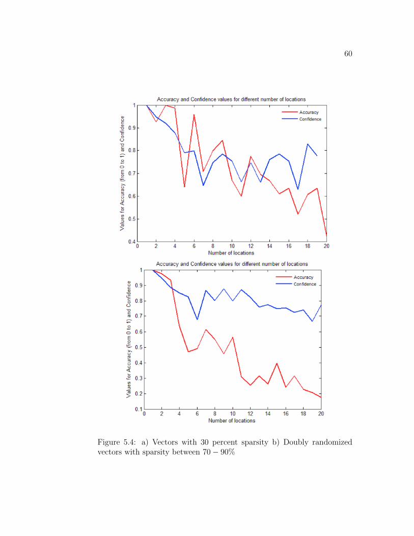
60

Figure 5.4: a) Vectors with 30 percent sparsity b) Doubly randomizedvectors with sparsity between 70− 90%

61

only are the bits chosen with a probability of 0.5, the percentage of

the vector that is 0/1 is also randomized (figure 5.4).

5.2.2 Hopfield Net

Memories are retained as stable entities or Gestalts and can be correctly

re-called from any reasonably sized subpart. The bridge between simple

circuits and the complex computational properties of higher nervous sys-

tems may be the spontaneous emergence of new computational capabilities

from the collective behavior of large numbers of simple processing elements

[Hopfield, 2006]. The Hopfield net is a recurrent artificial neural network

that serves as a content-addressable memory. The state of the network

has a scalar energy value associated with it. It is trained on binary repre-

sentations which occupy lower-energy states in the high-dimensional input

state space. An input to the network will gravitate towards these stored

patterns.

Implementation:

I used the MATLAB recipe for the Hopfield network that is based

on research by Li et al. They have studied a system that has the basic

structure of the Hopfield network is “easier to analyze, synthesize, and

implement than the Hopfield model.” [Li, 1989]. The MATLAB Hopfield

Net implementation uses the satlins function. For inputs less than -1

satlins produces -1. For inputs in the range -1 to +1 it simply returns the

input value. For inputs greater than +1 it produces +1. The input p to

the network specifies the initial conditions for the recurrent network. The

62

output of the network is fed back to become the input until it stabilizes

(see figure 5.5).

Figure 5.5: Hopfield Net: The output of the network is recursively fedback as input till the network stabilizes

I trained a Hopfield network on a set of target equilibrium points rep-

resented as a matrix T of vectors. The weights and biases for a recursive

Hopfield network were changed during the training phase, suggesting that

learning has happened. The network is guaranteed to have stable equi-

librium points at the target vectors, but it could contain other spurious

equilibrium points as well. In an autoassociative memory, concepts share

the same set of connections. By using inputs that are orthogonal or as

close to orthogonal as possible, we can optimally reduce the amount of

cross talk between different stored patterns [Hinton, 1989].

Figure 5.6 shows an orthogonal distribution of 50 hundred-dimensional

63

vectors used to train the network. Mutated versions of these were used

as testing samples. The network was successful in retrieving the stored

patterns.

Figure 5.6: Hopfield Net: The left hand and right hand figures depict thetraining samples and the output respectively. The red and blue regionssignify an activation value of 1 and 0 respectively for that unit. Thenetwork was trained on 50 orthogonal patterns each represented along onecolumn of the two dimensional plot. It successfully retrieved the storedpatterns.

Chapter 6

Event Related Potential

Experiment

6.1 Introduction

The firing of neurons is accompanied by change in the electrical potential

across the cell membrane. Event Related Potential (ERP) is an electro-

physiological technique used to record evoked potentials on the scalp in

response to a stimulus or directly after a cognitive response. The most

commonly used type of event ERP studies record visual evoked poten-

tials which are elicited in response to a visual presentation. ERPs have

high temporal resolution (1ms or better under optimal conditions) but

poor spatial resolution [Luck, 2005]. A comparison of the latency and

amplitude of the evoked potentials across the different experimental con-

ditional is done to find evidence for neural correlates of mental activ-

ity. Previous studies have discovered that our attention gravitates to-

64

65

wards specific spatial locations that are sustained in the working memory

[Awh et al., 1998, Awh and Jonides, 2001]. I designed and conducted an

ERP study to explore the attentional orientation towards maps at differ-

ent scales while actively thinking about a certain path. The purpose of

this study is to test the hierarchical spatial reasoning paradigm at a high

level.

6.2 Methods and Procedures

The first ingredient required to test spatial reasoning is a spatial map.

Since the subjects were mostly students at Hampshire College, we consid-

ered using the campus map. We found a more appealing alternative - a

virtual 3D world consisting of locations at different scales (shown in figure

6.1). This controls for potential bias due to varying degrees of familiarity

with the environment. This was also considered a better choice than us-

ing maps at different locations which would introduce hierarchical bias in

the initial exposure to the environment. Moreover, being allowed to roam

around in a virtual world during the somewhat long process of placing the

electrode cap kept the participants engaged and attentive.

6.2.1 Training Phase

The ERP design is based on the subjects’ ability to reason about and

visualize paths between two locations. A number of buildings are situated

in the vicinity of each other. A turquoise fountain, a gazebo and a mailbox

are placed at strategic locations to orient the player. Two of the buildings

66

Figure 6.1: Virtual 3D environment explored by the participants.

have open entrances. The rooms within the building are marked with

shapes of certain colors that serve as landmarks. The participants are

provided helpful suggestions such as asking them to find their way to a

central location such as the fountain from where both the open buildings

are visible. After the exploration phase, the subjects are trained on a series

of pathfinding problems involving a pair of landmarks. These are either

both within the same building or in separate buildings. When they are

in separate buildings, the participant must go up a scale to visualize the

path across the neighborhood.

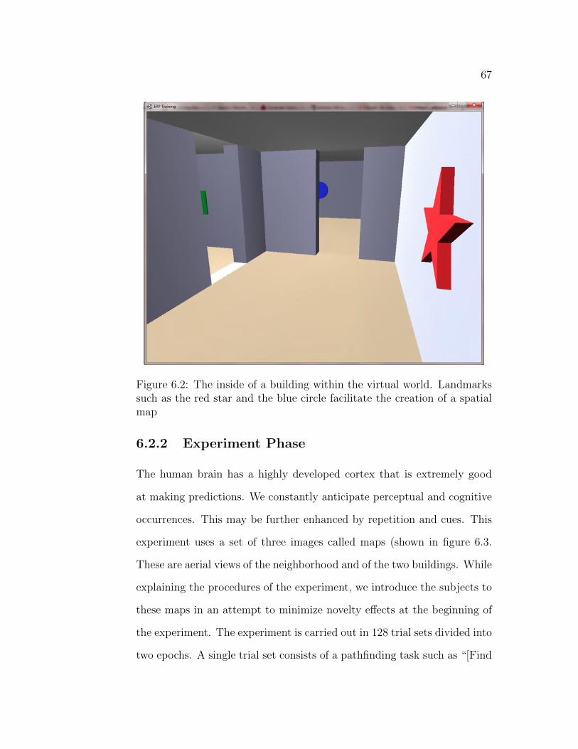
67

Figure 6.2: The inside of a building within the virtual world. Landmarkssuch as the red star and the blue circle facilitate the creation of a spatialmap

6.2.2 Experiment Phase

The human brain has a highly developed cortex that is extremely good

at making predictions. We constantly anticipate perceptual and cognitive

occurrences. This may be further enhanced by repetition and cues. This

experiment uses a set of three images called maps (shown in figure 6.3.

These are aerial views of the neighborhood and of the two buildings. While

explaining the procedures of the experiment, we introduce the subjects to

these maps in an attempt to minimize novelty effects at the beginning of

the experiment. The experiment is carried out in 128 trial sets divided into

two epochs. A single trial set consists of a pathfinding task such as “[Find

68

Figure 6.3: From left to right: Map of Building 1, 2 and the neighborhood.The first two are locations at scale 0 while the neighborhood is at scale 1

your way from] the blue square to the green triangle” followed by 3 trials.

During a trial, the participant is shown one of the three maps and asked

to indicate whether it is helpful in visualizing the path (1 for helpful and

2 for not helpful). The three maps are shown in a random order within

each trial set. During a particular trial set, the pathfinding task is chosen

randomly from a set of 16 tasks. There are two such distinct sets, one for

each epoch. A few sample pathfinding tasks are shown in table 6.1. In

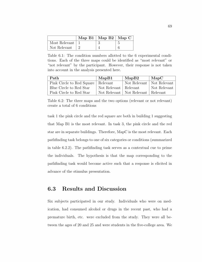
69

Map B1 Map B2 Map CMost Relevant 1 3 5Not Relevant 2 4 6

Table 6.1: The condition numbers allotted to the 6 experimental condi-tions. Each of the three maps could be identified as “most relevant” or“not relevant” by the participant. However, their response is not takeninto account in the analysis presented here.

Path MapB1 MapB2 MapCPink Circle to Red Square Relevant Not Relevant Not RelevantBlue Circle to Red Star Not Relevant Relevant Not RelevantPink Circle to Red Star Not Relevant Not Relevant Relevant

Table 6.2: The three maps and the two options (relevant or not relevant)create a total of 6 conditions

task 1 the pink circle and the red square are both in building 1 suggesting

that Map B1 is the most relevant. In task 3, the pink circle and the red

star are in separate buildings. Therefore, MapC is the most relevant. Each

pathfinding task belongs to one of six categories or conditions (summarized

in table 6.2.2). The pathfinding task serves as a contextual cue to prime

the individuals. The hypothesis is that the map corresponding to the

pathfinding task would become active such that a response is elicited in

advance of the stimulus presentation.

6.3 Results and Discussion

Six subjects participated in our study. Individuals who were on med-

ication, had consumed alcohol or drugs in the recent past, who had a

premature birth, etc. were excluded from the study. They were all be-

tween the ages of 20 and 25 and were students in the five-college area. We

70

rejected the ERP data for one subject as it contained too many artifacts

such as eye blinks and muscle movement. The waveforms shown in figure

6.4 was recorded from the electrodes above the occipital lobe where visual

information is processed. The waveforms peak around 100ms and another

around 220ms. The second peak is of greater interest since it occurred after

the purely visual response and thus may reflect a higher level conceptual

response.

The waveforms were imported into excel and then into SPSS for sta-

tistical analysis. There was a significant within-subject effect, i.e., the

participants’ evoked potentials were significantly different between the dif-

ferent conditions (Huynh-Feldt measure, p < 0.05). A Paired samples T

test was conducted (see figure 6.5) and significant differences were found

between Pair 1 (comparing conditions 1 and 2) (t=-3.301, p=0.03). The

evoked potentials to the Map B1 was significantly different between the

conditions where it was relevant and not relevant to the pathfinding task.

This indicates that the pathfinding task did influence the mental state

of the participants while we recorded their neural/cognitive response to

the image. As expected, there was no difference at all between conditions

2 and 4 (t=-0.408, p=0.704), when the maps B1 and B2 were both ir-

relevant. We know that map C contained the entire neighborhood and

is therefore always relevant to some extent. This is also empirically ob-

served as no significant difference is observed between conditions 5 and 6

(t=0.616, p=0.571). However, a comparison of conditions 1 and 6 shows

that the evoked ERPs when the map B1 were relevant was significantly

different from those evoked when the map C was not relevant (t=-2.821,

71

p=0.048). This suggests that although C was relevant to a greater or lesser

extent in all the pathfinding tasks, its activation may have been suppressed

when Map B1 was more relevant. When one entity exerts positive inhi-

bition on another, it points to the possibility that they are a part of the

same circuitry. This is an exploratory study with five subjects and not

very many trials each subject. The evidence in support of the hierarchical

reasoning paradigm is encouraging. We expect to see greater differences

in the conditions in a follow-up study with more subjects.

72

Figure 6.4: Grand Average ERP Waveforms: These waveforms were cre-ated by averaging together the averaged waveforms of the individual sub-jects across the different trials. These recordings are from the corticalareas above the occipital lobe, the visual processing region.

73

Figure 6.5: The Paired Samples T test is used to compare the conditionspair-wise. Significant differences were found for Pair 1 and Pair 7 (p <0.05). Refer to table 6.1 for the experimental conditions corresponding tothe condition numbers.

Chapter 7

Conclusions and Future Work

To recapitulate, this thesis presents a novel model of hierarchical spatial

reasoning using Holographic Reduced Representations. The nodes of the

tree are content addressable which allows this framework to support effi-

cient hierarchical search. This avoids the problem of explosion in the cog-

nitive load that hounds some other hierarchical models. The distributist

framework affords many advantages to this model such as automatic gen-

eralization, robustness in case of damaged or corrupted neural codes and

graceful degradation with increase in the number of locations. The bind-

ing operation is flexible owing to its useful properties of commutativity,

associativity, distributivity, stochasticity and self-inverse. This model has

many desirable properties such as fixed size of recursively composed neu-

ral codes, efficient path finding and scalability to large environments. For

all these reasons it is an attractive cognitive model of hierarchical spatial

reasoning.

This model of path finding captures the spirit of Hinton’s reduced de-

74

75

scription (shown below) [Hinton, 1990] although it is not an exact imple-

mentation.

1. Representational adequacy: The vector representing the loca-

tions (reduced description) cannot be used directly to retrieve all

the compositional keys and locations. However it can be queried to

retrieve information regarding the constituting locations.

2. Reduction: The full description of a location involves many keys

and locations at smaller scales. The reduced description is the same

size as any one of these constituents and thus satisfies the necessity

for reduction.

3. Systematicity: The reduced description for locations are system-

atically related to its constituting keys and locations, as described

by the compositional rules in Chapters 3 and 4.

4. Informativeness: X ⊗ Y will return a high similarity in the packed

hierarchy memory iff X is a location contained within Y at any hi-

erarchical level. Thus the locations are explicit in that they support

immediate accessibility. It is possible to probe a location once to

obtain information about smaller locations at any hierarchical level.

I would like to improve upon the model to support learning of represen-

tations using external data. I’m also interested in exploring an extension of

this model to more general environments and to three dimensions. Often,

the same environment can have competing hierarchical representations. I

76

wish to research into the framework and strategies for ensuring optimal

results in these cases.

Appendix A

Derivation of δ(X,A)

δ(X,A) is the probability that the corresponding bits of X and A are dif-

ferent. Let X = [A + B + ... + D(+R)]. Where A,B . . . ,D are K binary

vectors. The square brackets stand for the thresholding operation - each

bit of the vector X will be 0 or 1 depending on which of them appears more

frequently in that position among the K vectors. (In case K is even, a ran-

dom vector is added to X in case to make K odd). This section presents

the proof for δ(X,A) = 12− 1

2K

(K−1K−1

2

)For K= 1, δ(X,A) = 0. For K= 3, one out of the four combinations

(shown below) is such that A is 0 and X is 1, hence δ(X,A) = 0.25.

The following derivation is applicable to cases where K > 1. Let us

consider a bit at a particular location in the vectors A,B,D,R,X. Let m

be all possible combinations where A is 0 and X is 1 and n = all possible

combinations where A is 0.

δ(X,A) =m

n

77

78

For K= 1,δ(X,A) = 0, the total number of possible combinations where

A is 0 can be found by finding all the combinations of the remaining K-1

bits. This is given by the sum of all the elements of the (K − 1)th row of

the Pascal’s triangle. Hence we find the number of possible combinations

where A is 0 as: 2K−1

Since X is 1, there must be at least K+12

of the K − 1 bits must be 1

(since A is 0). Hence, to find all possible combinations where A=0 and

X=1, we consider all combinations such that exactly K+12

are 1, exactly

K+32

bits are 1, and so on.

Let(K−1K+1

2

)+(K−1K+3

2

)+ . . .+

( K−1K+2K−3

2 +1

2

)= x. Then 2x+

(K−1K−1

2

)= sum of all

elements of row (K − 1) of Pascals triangle = 2K−1

⇒ x = δ(X,A) =2K−1

2− 1

2

(K − 1K−12

)(A.1)

Using n= 2K−1 and (A.1) to get the expression for delta:

δ(X,A) =δ(X,A) = 2K−1

2− 1

2

(K−1K−1

2

)2K−1

⇒ δ(X,A) =1

2− 1

2K

(K − 1K−12

)

Appendix B

Pathfinding Example

Figure B.1: Spatial hierarchy depicted in graph-form. In this example,there are 18 locations at the most refined scale, which are grouped into 6locations at scale 1, 2 locations at scale 2 and 1 location at scale 3

B.1 Binary Framework Example

Locations at scale n in the location hierarchy is denoted by λ(n− i), where

n denotes the scale and i denotes an index value for the location at the

scale. Hence, leaf nodes are represented as λ(0 − i). Leaf nodes are clus-

79

80

tered to obtain scale 1 locations such as λ(1 − 1), λ(1 − 2) etc which are

further clustered into scale 2 locations such as λ(2 − 1) and λ(2 − 2). In

the example shown above the locations at scale 1 are generated from the

locations vectors as:

λ(1− 1) = κ(1− 1)⊗ (λ(0− 1) + λ(0− 2) + λ(0− 3) + λ(0− 4))

λ(1− 2) = κ(1− 2)⊗ (λ(0− 5) + λ(0− 6) + λ(0− 7) + λ(0− 8))

λ(1− 3) = κ(1− 3)⊗ (λ(0− 9) + λ(0− 10) + λ(0− 11) + λ(0− 12))

λ(1− 4) = κ(1− 4)⊗ (λ(0− 13) + λ(0− 14) + λ(0− 15) + λ(0− 16))

λ(1− 5) = κ(1− 5)⊗ (λ(0− 17) + λ(0− 18) + λ(0− 19) + λ(0− 20))

λ(1− 6) = κ(1− 6)⊗ (λ(0− 21) + λ(0− 22) + λ(0− 23) + λ(0− 24))

A location at scale 2 such as λ(2− 1) contains 3 scale 1 and 6 scale 1 lo-

cations which implies that k = 3 and m = 6. Using the expression above,

we get the following scale 2 locations:

λ(2− 1) = κ(2− 1)⊗ (λ(1− 1) + λ(1− 2) + λ(1− 3))

λ(2− 2) = κ(2− 2)⊗ (λ(1− 4) + λ(1− 5) + λ(1− 6))

A scale 3 location contains two scale 2 locations and there are a total of

two scale 2 locations giving us one location at scale 3:

λ(3− 1) = κ(3− 1)⊗ (λ(2− 1) + λ(2− 2))

Let us randomly assign λ(0 − 1) as the start location and λ(0 − 17)

as the goal location. We begin with the knowledge of the state vectors

corresponding to the start and the goal locations: µ(0− 1), λ(0− 1), and

µ(0−17), λ(0−17). We probe the current location λ(0−1) with µ(0−17).

The packed hierarchy memory is queried with µ(0 − 17) ⊗ λ(0 − 1) =

µ(0 − 17) ⊗ κ(0 − 1) ⊗ µ(0 − 1). This does not return a high similarity

81

value. So we go to the next higher scale. The current location at the next

scale is retrieved in two steps:

1. The packed hierarchy memory is queried with the current location

λ(0−1). The following item in the memory will have a high similarity

and will be returned:

PH = λ(0− 1) + λ(0− 1)⊗ λ(1− 1) + λ(0− 1)⊗ λ(1− 1)⊗ λ(2−

1) + λ(0− 1)⊗ λ(1− 1)⊗ λ(2− 1)⊗ λ(3− 1)

2. The location at the next scale is retrieved by querying the Location

memory with

λ(0− 1)⊗ PH = λ(0− 1)⊗ (λ(0− 1) + λ(0− 1)⊗ λ(1− 1)

+ λ(0− 1)⊗ λ(1− 1)⊗ λ(2− 1) + λ(0− 1)⊗

λ(1− 1)⊗ λ(2− 1)⊗ λ(3− 1))

= 0 + λ(1− 1) + λ(1− 1)⊗ λ(2− 1)

+ λ(1− 1)⊗ λ(2− 1)⊗ λ(3− 1)

∼ λ(1− 1)

The location at the next scale — λ(1 − 1) will be returned with a

high similarity in the location memory.

Now, the packed hierarchy memory is queried using µ(0− 17):

82

µ(0− 17)⊗ λ(1− 1) = µ(0− 17)⊗ (κ(1− 1)⊗ (µ(0− 1) + µ(0− 2)

+ µ(0− 3) + µ(0− 4)))

No item in the packed hierarchy memory has a high similarity to this

expression. Hence, we expand to the next scale λ(2−1) and probe it using

µ(0− 17) again:

µ(0− 17)⊗ λ(2− 1) = µ(0− 17)⊗ (κ(2− 1)⊗ (λ(1− 1) + λ(1− 2) + λ(1− 3)))

= µ(0− 17)⊗ (κ(2− 1)⊗ (κ(1− 1)⊗ (λ(0− 1) + λ(0− 2)

+ λ(0− 3) + λ(0− 4)) + κ(2− 1)⊗ (κ(1− 2)⊗

(λ(0− 5) + λ(0− 6) + λ(0− 7) + λ(0− 8))) + κ(2− 1)⊗

(κ(1− 3)⊗ (λ(0− 9) + λ(0− 10) + λ(0− 11) + λ(0− 12)))

Once again none of the terms will be recognizable in the packed hier-

archy memory so we expand to the next scale λ(3 − 1) which is probed

with the goal.

83

µ(0− 17)⊗ λ(3− 1) = µ(0− 17)⊗ (κ(3− 1)⊗ (λ(2− 1) + λ(2− 2)))

= µ(0− 17)⊗ (κ(3− 1)⊗ (κ(2− 1)⊗ (λ(1− 1) + λ(1− 2)

+ λ(1− 3))

+ κ(3− 1)⊗ (κ(2− 2)⊗ (λ(1− 4) + λ(1− 5) + λ(1− 6)))

= µ(0− 17)⊗ (κ(3− 1)⊗ (κ(2− 1)⊗ λ(1− 1) + κ(2− 1)

⊗ λ(1− 2) + κ(2− 1)⊗ λ(1− 3))

+ κ(3− 1)⊗ (κ(2− 2)⊗ λ(1− 4) + κ(2− 2)⊗ λ(1− 5)

+ κ(2− 2)⊗ λ(1− 6))

(Distributivity of ⊗ over merge)

= µ(0− 17)⊗ κ(3− 1)⊗ κ(2− 1)⊗ λ(1− 1) + µ(0− 17)⊗ κ(3− 1)

⊗ κ(2− 1)⊗ λ(1− 2)

+ µ(0− 17)⊗ κ(3− 1)⊗ κ(2− 1)⊗ λ(1− 3) + µ(0− 17)

⊗ κ(3− 1)⊗ κ(2− 2)⊗ λ(1− 4)

+ µ(0− 17)⊗ κ(3− 1)⊗ κ(2− 2)⊗ λ(1− 5) + µ(0− 17)

⊗ κ(3− 1)⊗ κ(2− 2)⊗ λ(1− 6)

(Distributivity of ⊗ over merge)

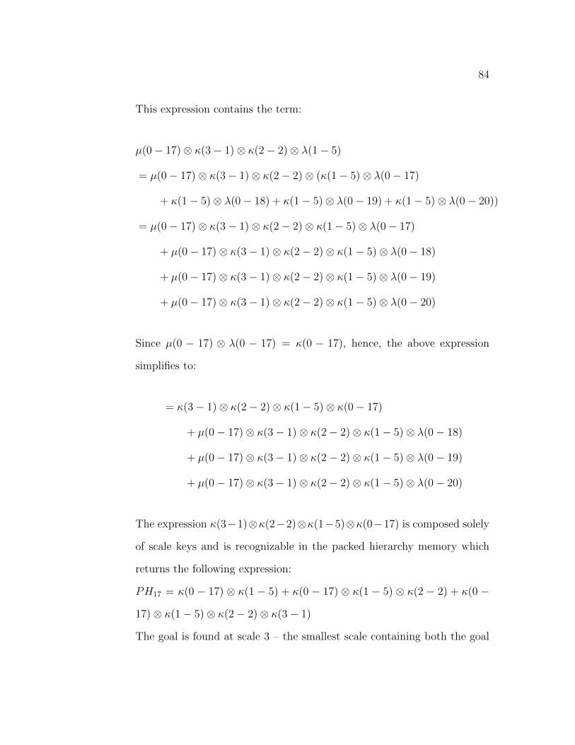
84

This expression contains the term:

µ(0− 17)⊗ κ(3− 1)⊗ κ(2− 2)⊗ λ(1− 5)

= µ(0− 17)⊗ κ(3− 1)⊗ κ(2− 2)⊗ (κ(1− 5)⊗ λ(0− 17)

+ κ(1− 5)⊗ λ(0− 18) + κ(1− 5)⊗ λ(0− 19) + κ(1− 5)⊗ λ(0− 20))

= µ(0− 17)⊗ κ(3− 1)⊗ κ(2− 2)⊗ κ(1− 5)⊗ λ(0− 17)

+ µ(0− 17)⊗ κ(3− 1)⊗ κ(2− 2)⊗ κ(1− 5)⊗ λ(0− 18)

+ µ(0− 17)⊗ κ(3− 1)⊗ κ(2− 2)⊗ κ(1− 5)⊗ λ(0− 19)

+ µ(0− 17)⊗ κ(3− 1)⊗ κ(2− 2)⊗ κ(1− 5)⊗ λ(0− 20)

Since µ(0 − 17) ⊗ λ(0 − 17) = κ(0 − 17), hence, the above expression

simplifies to:

= κ(3− 1)⊗ κ(2− 2)⊗ κ(1− 5)⊗ κ(0− 17)

+ µ(0− 17)⊗ κ(3− 1)⊗ κ(2− 2)⊗ κ(1− 5)⊗ λ(0− 18)

+ µ(0− 17)⊗ κ(3− 1)⊗ κ(2− 2)⊗ κ(1− 5)⊗ λ(0− 19)

+ µ(0− 17)⊗ κ(3− 1)⊗ κ(2− 2)⊗ κ(1− 5)⊗ λ(0− 20)

The expression κ(3−1)⊗κ(2−2)⊗κ(1−5)⊗κ(0−17) is composed solely

of scale keys and is recognizable in the packed hierarchy memory which

returns the following expression:

PH17 = κ(0 − 17) ⊗ κ(1 − 5) + κ(0 − 17) ⊗ κ(1 − 5) ⊗ κ(2 − 2) + κ(0 −

17)⊗ κ(1− 5)⊗ κ(2− 2)⊗ κ(3− 1)

The goal is found at scale 3 – the smallest scale containing both the goal

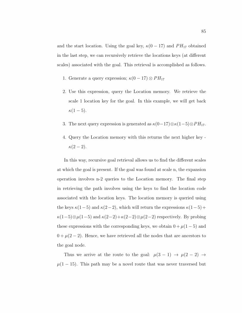
85

and the start location. Using the goal key, κ(0 − 17) and PH17 obtained

in the last step, we can recursively retrieve the locations keys (at different

scales) associated with the goal. This retrieval is accomplished as follows.

1. Generate a query expression; κ(0− 17)⊗ PH17

2. Use this expression, query the Location memory. We retrieve the

scale 1 location key for the goal. In this example, we will get back

κ(1− 5).

3. The next query expression is generated as κ(0−17)⊗κ(1−5)⊗PH17.

4. Query the Location memory with this returns the next higher key -

κ(2− 2).

In this way, recursive goal retrieval allows us to find the different scales

at which the goal is present. If the goal was found at scale n, the expansion

operation involves n-2 queries to the Location memory. The final step

in retrieving the path involves using the keys to find the location code

associated with the location keys. The location memory is queried using

the keys κ(1−5) and κ(2−2), which will return the expressions κ(1−5)+

κ(1−5)⊗µ(1−5) and κ(2−2)+κ(2−2)⊗µ(2−2) respectively. By probing

these expressions with the corresponding keys, we obtain 0 +µ(1− 5) and

0 + µ(2− 2). Hence, we have retrieved all the nodes that are ancestors to

the goal node.

Thus we arrive at the route to the goal: µ(3 − 1) → µ(2 − 2) →

µ(1 − 15). This path may be a novel route that was never traversed but

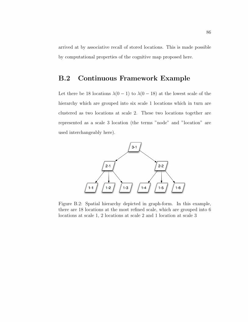
86

arrived at by associative recall of stored locations. This is made possible

by computational properties of the cognitive map proposed here.

B.2 Continuous Framework Example

Let there be 18 locations λ(0 − 1) to λ(0 − 18) at the lowest scale of the

hierarchy which are grouped into six scale 1 locations which in turn are

clustered as two locations at scale 2. These two locations together are

represented as a scale 3 location (the terms ”node” and ”location” are

used interchangeably here).

Figure B.2: Spatial hierarchy depicted in graph-form. In this example,there are 18 locations at the most refined scale, which are grouped into 6locations at scale 1, 2 locations at scale 2 and 1 location at scale 3

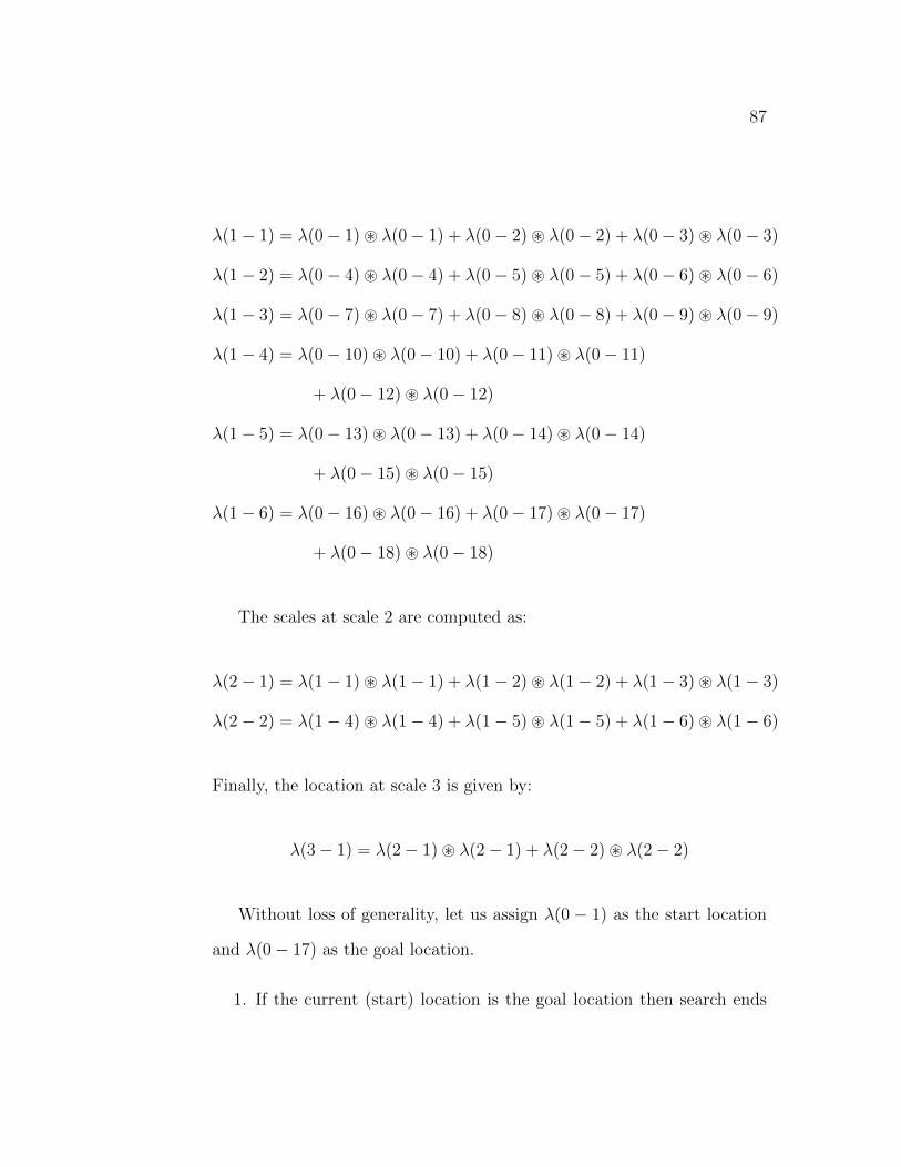
87

λ(1− 1) = λ(0− 1) ~ λ(0− 1) + λ(0− 2) ~ λ(0− 2) + λ(0− 3) ~ λ(0− 3)

λ(1− 2) = λ(0− 4) ~ λ(0− 4) + λ(0− 5) ~ λ(0− 5) + λ(0− 6) ~ λ(0− 6)

λ(1− 3) = λ(0− 7) ~ λ(0− 7) + λ(0− 8) ~ λ(0− 8) + λ(0− 9) ~ λ(0− 9)

λ(1− 4) = λ(0− 10) ~ λ(0− 10) + λ(0− 11) ~ λ(0− 11)

+ λ(0− 12) ~ λ(0− 12)

λ(1− 5) = λ(0− 13) ~ λ(0− 13) + λ(0− 14) ~ λ(0− 14)

+ λ(0− 15) ~ λ(0− 15)

λ(1− 6) = λ(0− 16) ~ λ(0− 16) + λ(0− 17) ~ λ(0− 17)

+ λ(0− 18) ~ λ(0− 18)

The scales at scale 2 are computed as:

λ(2− 1) = λ(1− 1) ~ λ(1− 1) + λ(1− 2) ~ λ(1− 2) + λ(1− 3) ~ λ(1− 3)

λ(2− 2) = λ(1− 4) ~ λ(1− 4) + λ(1− 5) ~ λ(1− 5) + λ(1− 6) ~ λ(1− 6)

Finally, the location at scale 3 is given by:

λ(3− 1) = λ(2− 1) ~ λ(2− 1) + λ(2− 2) ~ λ(2− 2)

Without loss of generality, let us assign λ(0 − 1) as the start location

and λ(0− 17) as the goal location.

1. If the current (start) location is the goal location then search ends

88

here (trivial case).

2. Else, we retrieve the location at the next higher scale, a.k.a. the

parent node.

3. We check whether this is the goal location and if it is not found, step

2 is repeated until the goal is found at some scale. Subsequently, the

ancestors of the goal node are retrieved.

The current location at the next scale is retrieved in two steps:

1. The packed hierarchy (PH) memory is queried with the current lo-

cation λ(0− 1). The following item in the memory will have a high

similarity and will be returned:

PH = λ(0− 1) + λ(0− 1) ~ λ(1− 1) + λ(0− 1) ~ λ(1− 1) ~ λ(2−

1) + λ(0− 1) ~ λ(1− 1) ~ λ(2− 1) ~ λ(3− 1)

2. Its parent is retrieved by querying the Location memory with λ(0−

1) ~ PH:

∼ λ(0− 1) ~ (λ(0− 1) + λ(0− 1) ~ λ(1− 1) + λ(0− 1) ~ λ(1− 1)

~ λ(2− 1) + λ(0− 1) ~ λ(1− 1) ~ λ(2− 1) ~ λ(3− 1))

∼ 0 + λ(1− 1) + λ(1− 1) ~ λ(2− 1) + λ(1− 1) ~ λ(2− 1)

~ λ(3− 1) λ(1− 1)

The location at the next scale — λ(1 − 1) will be returned with a

high similarity in the location memory.

89

Now, the packed hierarchy memory is queried using λ(0− 17)T :

λ(0− 17)T ~ λ(1− 1) = λ(0− 17)T ~ (λ(0− 1) ~ λ(0− 1) + λ(0− 2)

~ µ(0− 2) + λ(0− 3) ~ λ(0− 3) + λ(0− 4) ~ λ(0− 4)))

No item in the packed hierarchy memory has a high similarity to this

expression. Hence, we expand to the next scale λ(2−1) and probe it using

λ(0− 17) again:

λ(0− 17)T ~ λ(2− 1) ∼ λ(0− 17)T ~ (λ(1− 1) ~ λ(1− 1)

+ λ(1− 2) ~ λ(1− 2) + λ(1− 3) ~ λ(1− 3))

∼ λ(0− 17)T ~ (λ(1− 1) ~ (λ(0− 1) ~ λ(0− 1)

+ λ(0− 2) ~ λ(0− 2) + λ(0− 3) ~ λ(0− 3)

+ λ(0− 4) ~ λ(0− 4))

+ λ(1− 2) ~ (λ(0− 5) ~ λ(0− 5) + λ(0− 6) ~ λ(0− 6)

+ λ(0− 7) ~ λ(0− 7) + λ(0− 8) ~ λ(0− 8))

+ λ(1− 3) ~ (λ(0− 9) ~ λ(0− 9) + λ(0− 10) ~ λ(0− 10)

+ λ(0− 11) ~ λ(0− 11) + λ(0− 12) ~ λ(0− 12)))

Once again none of the terms will be recognizable in the packed hier-

archy memory so we expand to the next scale λ(3 − 1) which is probed

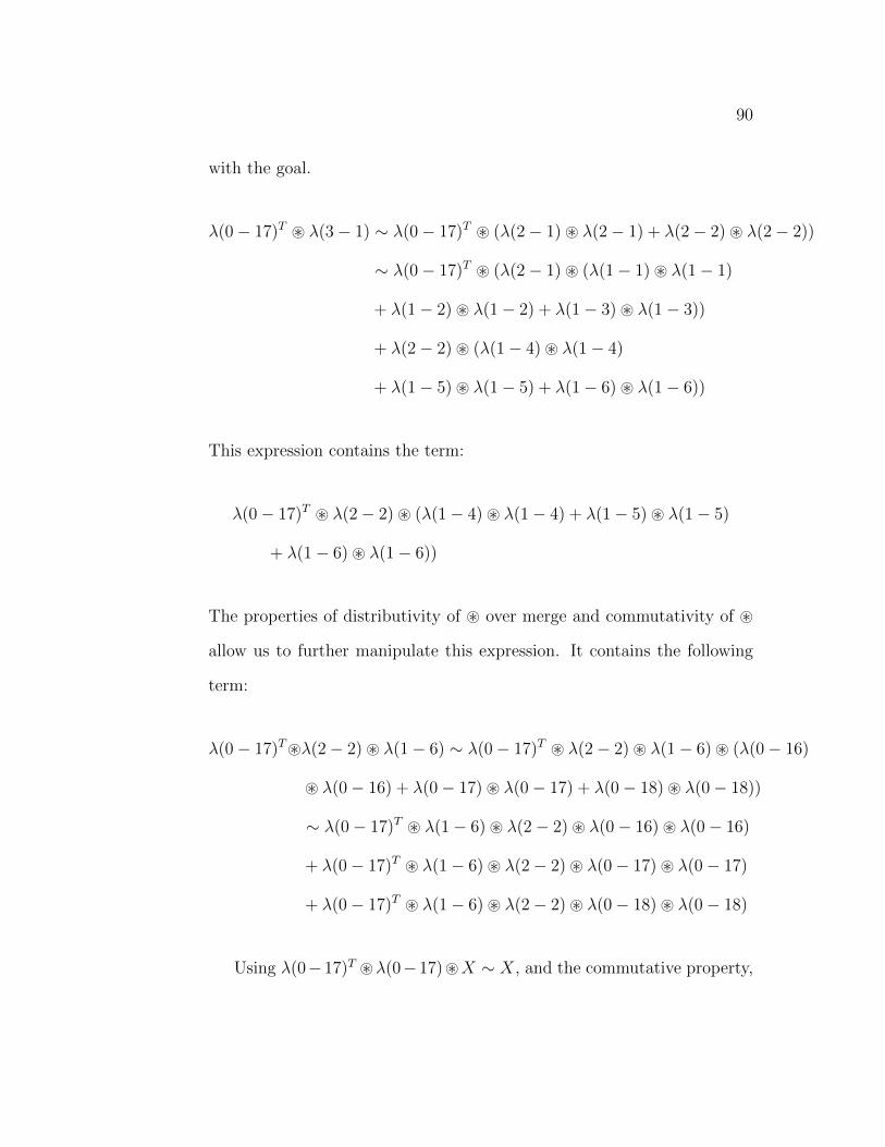
90

with the goal.

λ(0− 17)T ~ λ(3− 1) ∼ λ(0− 17)T ~ (λ(2− 1) ~ λ(2− 1) + λ(2− 2) ~ λ(2− 2))

∼ λ(0− 17)T ~ (λ(2− 1) ~ (λ(1− 1) ~ λ(1− 1)

+ λ(1− 2) ~ λ(1− 2) + λ(1− 3) ~ λ(1− 3))

+ λ(2− 2) ~ (λ(1− 4) ~ λ(1− 4)

+ λ(1− 5) ~ λ(1− 5) + λ(1− 6) ~ λ(1− 6))

This expression contains the term:

λ(0− 17)T ~ λ(2− 2) ~ (λ(1− 4) ~ λ(1− 4) + λ(1− 5) ~ λ(1− 5)

+ λ(1− 6) ~ λ(1− 6))

The properties of distributivity of ~ over merge and commutativity of ~

allow us to further manipulate this expression. It contains the following

term:

λ(0− 17)T~λ(2− 2) ~ λ(1− 6) ∼ λ(0− 17)T ~ λ(2− 2) ~ λ(1− 6) ~ (λ(0− 16)

~ λ(0− 16) + λ(0− 17) ~ λ(0− 17) + λ(0− 18) ~ λ(0− 18))

∼ λ(0− 17)T ~ λ(1− 6) ~ λ(2− 2) ~ λ(0− 16) ~ λ(0− 16)

+ λ(0− 17)T ~ λ(1− 6) ~ λ(2− 2) ~ λ(0− 17) ~ λ(0− 17)

+ λ(0− 17)T ~ λ(1− 6) ~ λ(2− 2) ~ λ(0− 18) ~ λ(0− 18)

Using λ(0−17)T ~λ(0−17)~X ∼ X, and the commutative property,

91

the above expression simplifies to:

∼ λ(0− 17)T ~ λ(1− 6) ~ λ(2− 2) ~ λ(0− 16) ~ λ(0− 16)

+λ(0− 17) ~ λ(1− 6) ~ λ(2− 2)

+λ(0− 17)T ~ λ(1− 6) ~ λ(2− 2) ~ λ(0− 18) ~ λ(0− 18)

The expression λ(0 − 17) ~ λ(1 − 6) ~ λ(2 − 2) does not contain any

auto-convolution terms. It is recognizable in the packed hierarchy memory

which returns the following expression:

PH17 = λ(0− 17) + λ(0− 17)~ λ(1− 6) + λ(0− 17)~ λ(1− 6)~ λ(2− 2)

The goal is found at scale 3 – the smallest scale containing both the goal

and the start location. Using the goal location, λ(0 − 17) and PH17 ob-

tained in the last step, we can recursively retrieve the locations at different

scales associated with the goal. This retrieval is accomplished as follows.

1. Generate the query expression; λ(0− 17) ~ PH17

2. Using this expression, query the Location memory to retrieve the

scale 1 goal node. In this example, we will retrieve λ(1− 5).

3. The next query expression is generated as λ(0−17)~λ(1−5)~PH17.

4. Query the Location memory to retrieve the next higher key - λ(2−2).

In this way, recursive goal retrieval allows us to find the ancestors of

the goal node. If the goal was found at scale n, the expansion operation

involves n− 2 queries to the Location memory.

92

B.3 Dimensionality

1000 2000 3000 4000 5000 6000 7000 8000 9000 100000.495

0.5

0.505

0.51

0.515

0.52

Sim

ilari

ty V

alu

es

Dimension of State Vector

Relationship of Accuracy and Con!dence values to dimension

AccuracyCon!dence

Figure B.3: Relationship of Accuracy and Confidence values to Dimen-sionality

The sensitivity of the pathfinding process to the number of units in the

distributed representation was examined. Since the number of possible n-

bit binary distributed representations are 2n, increasing the dimensionality

of our state vectors does not have a significant effect on the accuracy and

confidence values of pathfinding.

Bibliography

[Awh and Jonides, 2001] Awh, E. and Jonides, J. (2001). Overlappingmechanisms of attention and spatial working memory. Trends in Cog-nitive Sciences, 5(3):119–126.

[Awh et al., 1998] Awh, E., Jonides, J., Reuter-Lorenz, and Patricia, A.(1998). Rehearsal in spatial working memory. Journal of ExperimentalPsychology: Human Perception and Performance, 24(3):780–790.

[Car and Frank, 1994] Car, A. and Frank, A. (1994). General principlesof hierarchical spatial reasoning - the case of wayfinding. Proceedings ofthe Conference on Spatial Data Handling.

[Cohn et al., 2002] Cohn, A. G., Magee, D. R., Galata, A., Hogg, D. C.,and Hazarika, S. M. (2002). Towards an architecture for cognitive visionusing qualitative spario-temporal representations and abduction. In InSpatial Cognition III, pages 232–248. Springer-Verlag.

[Dolins and Mitchell, 2010] Dolins, F. L. and Mitchell, R. W. (2010). Spa-tial Cognition, Spatial Perception. Cambridge University Press., NewYork, NY, USA.

[Essen and Maunsell, 1983] Essen, D. C. V. and Maunsell, J. H. (1983).Hierarchical organization and functional streams in the visual cortex.Trends in Neurosciences, 6:370 – 375.

[Etienne and Jeffery, 2004] Etienne, A. S. and Jeffery, K. J. (2004). Pathintegration in mammals. Hippocampus, 14(2):180–192.

[Felleman and Van Essen, 1991] Felleman, D. J. and Van Essen, D. C.(1991). Distributed hierarchical processing in the primate cerebral cor-tex. Cerebral Cortex, 1(1):1–47.

[Hawkins and Blakeslee, 2004] Hawkins, J. and Blakeslee, S. (2004). OnIntelligence. Henry Holt and Company.

93

94

[Hinton, 1989] Hinton, G. E. (1989). Parallel Models of Associative Mem-ory. L. Erlbaum Associates Inc., Hillsdale, NJ, USA.

[Hinton, 1990] Hinton, G. E. (1990). Mapping part-whole hierarchies intoconnectionist networks. Artif. Intell., 46:47–75.

[Hopfield, 2006] Hopfield, J. J. (2006). Neural networks and physical sys-tems with emergent collective computational abilities. Proceedings ofThe National Academy of Sciences.

[Hopfield, 2010] Hopfield, J. J. (2010). Neurodynamics of mental explo-ration. Proceedings of the National Academy of Sciences, 107(4):1648–1653.

[Huang et al., 1997] Huang, Y.-W., Jing, N., and Rundensteiner, E.(1997). A hierarchical path view model for path finding inintelligent transportation systems. GeoInformatica, 1:125–159.10.1023/A:1009784527790.

[Kanerva, 1993] Kanerva, P. (1993). Associative Neural Memories: The-ory and Implementation, chapter Sparse Distributed Memory and Re-lated Models, pages 50–76. Number 3. Oxford University Press, NewYork, NY, USA.

[Kanerva, 1997] Kanerva, P. (1997). Fully distributed representation. Pro-ceedings of 1997 Real World Computing Symposium (Tokyo, Japan),pages 358–365.

[Kanerva, 1998] Kanerva, P. (1998). Dual role of analogy in the designof a cognitive computer. Advances in Analogy Research: Integration ofTheory and Data from the Cognitive, Computational, and Neural Sci-ences.

[Kubie and Fenton, 2008] Kubie, J. L. and Fenton, A. A. (2008). Heading-vector navigation based on head-direction cells and path integration.Hippocampus, 9999(9999).

[Li, 1989] Li, J. (1989). Analysis and synthesis of a class of neural net-works: linear system operating on a closed hypercube. IEEE Transac-tions on Circuits and Systems, 36:1405–1422.

[Luck, 2005] Luck, S. J. (2005). An introduction to the event-related po-tential technique. MIT Press, Cambridge, MA.

95

[McLeod et al., 1998] McLeod, P., Plunkett, K., and Rolls, E. T. (1998).Introduction to Connectionist Modeling of Cognitive Processes. OxfordUniversity Press, New York, NY, USA.

[Mollison, 2005] Mollison, M. (2005). Event-related potentials in humansduring spatial navigation. PhD thesis, Brandeis University, Waltham,MA, USA.

[O’Keefe and Nadel, 1978] O’Keefe, J. and Nadel, L. (1978). The hip-pocampus as a cognitive map. Clarendon Press.

[Plate, 2002] Plate, T. (2002). Distributed Representations. MacmillianEncyclopedia of Cognitive Science.

[Plate, 2003] Plate, T. (2003). Holographic reduced representation: dis-tributed representation for cognitive structures. CSLI lecture notes. CSLIPublications.

[Plate, 1991] Plate, T. A. (1991). Convolution algebra for compositionaldistributed representations. Proceedings of the 12th International JointConference on Artificial Intelligence, pages 30–35.

[Plate, 1995] Plate, T. A. (1995). Holographic reduced representations.IEEE Transactions on Neural Networks, 6(3).

[Plate, 2000] Plate, T. A. (2000). Analogy retrieval and processing withdistributed vector representations. Expert Systems: The InternationalJournal of Knowledge Engineering and Neural Networks, Special Issueon Connectionist Symbol Processing, 17(1):29–40.

[Rachkovskij, 2001] Rachkovskij, D. A. (2001). Representation and pro-cessing of structures with binary sparse distributed codes. IEEE Trans.on Knowl. and Data Eng., 13:261–276.

[Reese and Lipsitt, 1975] Reese, H. W. and Lipsitt, L. P. (1975). Advancesin child development and behavior. Academic Press Inc.

[Rohrbein et al., 2003] Rohrbein, F., Schill, K., Baier, V., Stein, K., Zet-zsche, C., and Brauer, W. (2003). Spatial cognition iii. chapter Motionshapes: empirical studies and neural modeling, pages 305–320. Springer-Verlag, Berlin, Heidelberg.

[Tolman, 1948] Tolman, E. C. (1948). Cognitive maps in rats and men.Psychological Review, 55(4):189–208.

96

[Widrow and Hoff, 1960] Widrow, B. and Hoff, M. E., J. (1960). Adaptiveswitching circuits. IRE WESCON Convention Record, 4:96–104.