PNNL-14256

Model Documentation The Second Generation Model Antoinette L. Brenkert Ronald D. Sands Son H. Kim Hugh M. Pitcher

October 2004 Prepared for the United States Environmental Protection Agency under Contracts AGRDW89939464-01 and AGRDW89939645-01 Joint Global Change Research Institute, College Park, MD Pacific Northwest National Laboratory Operated by Battelle for the US Department of Energy

LEGAL NOTICE This report was prepared by Battelle Memorial Institute (Battelle) as an account of sponsored research activities. Neither Client nor Battelle nor any person acting on behalf of either: MAKES ANY WARRANTY OR REPRESENTATION, EXPRESS OR IMPLIED, with respect to the accuracy, completeness, or usefulness of the information contained in this report, or that the use of any information, apparatus, process, or composition disclosed in this report may not infringe privately owned rights; or Assumes any liabilities with respect to the use of, or for damages resulting from the use of, any information, apparatus, process, or composition disclosed in this report. Reference herein to any specific commercial product, process, or service by trade name, trademark, manufacturer, or otherwise, does not necessarily constitute or imply its endorsement, recommendation, or favoring by Battelle. The views and opinions of authors expressed herein do not necessarily state or reflect those of Battelle.

Printed in the United States of America

3

Executive Summary For a full overview of the model see the “SGM Model Overview”. Briefly, the Second Generation Model (SGM) is a computable general equilibrium model designed specifically to analyze issues related to energy, economy, and greenhouse gas emissions. It has 14 global regions, multiple greenhouse gas emissions, vintaged capital stocks, explicit connections between technology and the economy, disaggregated to reflect the relative importance of sectors in determining greenhouse gas emissions, and explicit treatment of energy and land stocks. Model development began in 1991. The first model design paper was published in 1993 (Edmonds, et al., 1993). The SGM was developed to complement the “first generation model,” referred to as the MiniCAM. The MiniCAM was also explicitly designed to address long-term, strategic, issues related to energy, economy, and greenhouse gas emissions (Edmonds and Reilly, 1983)1 and continues to be used for that purpose2. In contrast the SGM was designed to address transitional energy-economy-technology-greenhouse-gas-emissions issues. The detailed documentation below presents the SGM 2003 version. The SGM was developed at the Pacific Northwest National Laboratory (PNNL) and is maintained by the PNNL Joint Global Change Research Institute (JGCRI)3.

1 The MiniCAM evolved to include agriculture, land-use, terrestrial and ocean carbon cycle, radiative forcing, sea level rise, and climate change. 2 For a brief comparison between the SGM and MiniCAM see Appendix D 3 The JGCRI is a collaboration between the PNNL and the University of Maryland at College Park. The JGCRI is located on the campus of the University of Maryland in College Park, MD.

4

Acknowledgments We want to thank Elizabeth L. Malone for steadfast support and for editing the document. We want to thank Marshall Wise and Joe M. Roop for their peer review. We want to thank the Economic Analysis Branch of the Office of Atmospheric Programs of the Environmental Protection Agency’s Climate Change Division for making this documentation become reality.

5

Table of Contents LEGAL NOTICE ............................................................................................................................ 2 Executive Summary ........................................................................................................................ 2 Acknowledgments ........................................................................................................................... 2

Table of Contents.................................................................................................................... 2 List of Figures......................................................................................................................... 2 List of Tables........................................................................................................................... 2

Chapter 1. The Second Generation Model ...................................................................................... 2 Chapter 2. The modeling framework: economic input-output and energy balance tables ............. 2

Production and input-output tables in the SGM..................................................................... 2 Investment and capital stocks ................................................................................................. 2

Chapter 3. Production functions ..................................................................................................... 2 Production functions, vintages, and the input-output matrix ................................................. 2 CES production by vintage ..................................................................................................... 2 Long- and short-run elasticities.............................................................................................. 2 The Leontief or fixed coefficient production function............................................................. 2

Chapter 4. Prices and expected prices ............................................................................................. 2 Base year prices and initial future prices............................................................................... 2 Determining prices paid for supplies by producers, prices received for produced commodities, and policy potential .......................................................................................... 2 Expected prices....................................................................................................................... 2

Chapter 5. Technical change ........................................................................................................... 2 Input-output coefficients and their relationship to the technical scale coefficients................ 2 How technical change is operationalized in the SGM............................................................ 2 The technical coefficients (αi,j) in the CES production function............................................. 2 The technical coefficients (λi,j) in the Leontief production function ....................................... 2

Chapter 6. Profits, demands, expected profit rates, and the operation of capital ........................... 2 Profits and the production functions ...................................................................................... 2

Profits and the CES production function............................................................................ 2 Profits and the Leontief production function...................................................................... 2

The relationship between profits and demands ...................................................................... 2 Demands and the CES production function ....................................................................... 2 Demands and the Leontief production function ................................................................. 2

Expected profit rates............................................................................................................... 2 Operation of capital stock in the SGM: determining production and interindustry demand . 2

Old vintages........................................................................................................................ 2 New vintages ...................................................................................................................... 2 Demands by production sectors and cost calculations ....................................................... 2 Additional costs when operating any of the active vintages .............................................. 2

Chapter 7. Carbon policies .............................................................................................................. 2 Carbon prices and revenue cycling ........................................................................................ 2 Carbon permit trade ............................................................................................................... 2 Carbon policy impacts ............................................................................................................ 2

Chapter 8. The final demand sectors ............................................................................................... 2

6

Investment ............................................................................................................................... 2 Households ............................................................................................................................. 2 Government............................................................................................................................. 2 Imports and exports ................................................................................................................ 2

Chapter 9. GNP accounting............................................................................................................. 2 Chapter 10. The solution procedure ................................................................................................ 2 Chapter 11. Calibration procedure .................................................................................................. 2 Chapter 12. The energy balance and emissions............................................................................... 2

Fossil fuel emissions ............................................................................................................... 2 Other greenhouse gas emissions and non-greenhouse gases ................................................. 2 Mitigation and marginal abatement cost curves .................................................................... 2 Display of results .................................................................................................................... 2

Chapter 13. Reference case results .................................................................................................. 2 Projections/Validation/Calibration for the USA .................................................................... 2

References ....................................................................................................................................... 2 List of Equations ............................................................................................................................. 2

7

List of Figures Figure 1 The flow of goods and services in SGM........................................................................... 2 Figure 2 Typical input-output table................................................................................................. 2 Figure 3 Typical energy balance table............................................................................................. 2 Figure 4 Basic flowchart of the SGM model................................................................................... 2 Figure 5 Annual investment: paper making and paper products in China ...................................... 2 Figure 6 Putty-semiputty isoquants ................................................................................................. 2 Figure 7 Putty-clay isoquants .......................................................................................................... 2 Figure 8 Neutral technical change when the elasticity of substitution coefficient (σ) equals 0.5... 2 Figure 9 Biased technical change when the elasticity of substitution coefficient (σ) equals 0.5 .... 2 Figure 10 Investment into production sectors over time ................................................................. 2 Figure 11 Investments in fossil fuel related production over time .................................................. 2 Figure 12 Investment in electricity production over time ............................................................... 2 Figure 13 Quantities of uninvested depletable resources and invested capital in depletable

resources for one region in a case other than the reference case illustrating the well-behaved nature of the SGM .................................................................................................................. 2

Figure 14 Marginal abatement cost curves for the United States energy system generated with a series of constant-carbon-price experiments........................................................................... 2

Figure 15 Historical and projected normalized GNP ...................................................................... 2 Figure 16 CO2 emissions in units of million tons of carbon in the reference case with a zero

carbon fee and the responses of CO2 emissions to carbon fees of $10, $50, $100, and $200 per ton carbon ......................................................................................................................... 2

Figure 17 Response of CO2 and carbon-equivalent emissions in units of million tons of carbon to carbon fees of $100 per ton carbon......................................................................................... 2

Figure 18 Response of CO2 emissions in units of million tons of carbon from oil, gas, and coal combustion to carbon fees of zero versus $100 per ton carbon.............................................. 2

Figure 19 Response of carbon-equivalent emissions in units of million tons of carbon from energy production, energy transformation, agricultural and other production processes to carbon fees of zero versus $100 per ton carbon ................................................................................. 2

Figure 20 Response of carbon-equivalent emissions in units of million tons of carbon from agricultural processes to carbon fees of zero versus $100 per ton carbon.............................. 2

Figure 21 Carbon-equivalent emissions in units of million tons of carbon from industrial processes responding to carbon fees....................................................................................... 2

Figure 22 Emission stabilization levels in units of million tons of carbon set exogenously and reached as model output ......................................................................................................... 2

Figure 23 Market prices for carbon when exogenously set emission stabilization levels are attained. Note that the steep curve is for the carbon price when only energy production and agricultural carbon-equivalent emissions are mitigated but for landfills; no industrial emissions are mitigated........................................................................................................... 2

Figure 24 Emission pathways due to the energy sectors when carbon-equivalent emission limits are imposed............................................................................................................................. 2

Figure 25 Emission pathways due to the agricultural sector when carbon-equivalent emission limits are imposed................................................................................................................... 2

8

Figure 26 The vintage-specific (vin-3 through vin-0) technical scale coefficients over time that relate the agricultural input to production in the reference case ............................................. 2

Figure 27 The vintage-specific technical scale coefficients (vin-3 through vin-0) over time that relate the agricultural input to production. The vintage-specific technical scale coefficients are shown (1) when all sectors are impacted by a carbon price and all carbon-equivalent emissions are mitigated (CE_all) and (2) when all sectors are impacted by a carbon price and the energy production sectors and a limited number of agricultural processes are mitigated (CE_ind) (no landfill mitigation and no industrial processes mitigation). ............. 2

Figure 28 Historical and projected electricity generation in the USA. in billion kilowatt hours .... 2 Figure 29 Historical and projected CO2 emissions in units of million tons of carbon from the

combustion of fossil fuels from electricity generation ........................................................... 2 Figure 30 CO2 emissions in units of million tons of carbon from the combustion of fossil fuels

from electricity generation...................................................................................................... 2 Figure 31 CO2 emissions in units of million tons of carbon from the combustion of fossil fuels

from electricity generation when carbon fees are imposed of $100 per ton carbon ............... 2

List of Tables Table 1 Regions in the SGM ........................................................................................................... 2 Table 2 Production sectors and sub-sectors in SGM 2003.............................................................. 2 Table 3 Relationship between vintages (v) and times of operation (t) ............................................ 2 Table 4 Variable values at the end of the last iteration of the market solving algorithms when

carbon policies are based on carbon emission limits .............................................................. 2 Table 5 Emissions sources, drivers and control options.................................................................. 2

9

Chapter 1. The Second Generation Model The Second Generation Model (SGM) is a computable general equilibrium model designed specifically to analyze issues related to energy, economy, and greenhouse gas emissions. It has 14 global regions, multiple greenhouse gas emissions, vintaged capital stocks, explicit connections between technology and the economy, disaggregated to a degree to reflect the relative importance of sectors in determining greenhouse gas emissions. The SGM is maintained at the Joint Global Change Research Institute, operated by Pacific Northwest National Laboratory and the University of Maryland. The SGM projects economic activity, energy consumption, and greenhouse gas emissions for each region in five-year time steps from 1990 through 2050. It is designed specifically to address issues associated with global change, including (1) projecting baseline carbon-equivalent emissions over time for a country or group of countries; (2) determining the least-cost way to meet any particular emissions constraint; (3) providing a measure of the carbon price, in dollars per metric ton carbon; and (4) providing a measure of the overall cost of meeting an emissions target. Below we present a quick overview of the chapters that follow. The chapters describe in detail all model processes simulated in SGM 2003. Chapter two explicates two basic features of the SGM: the basic structure of the SGM, that is, the regional hybrid commodity-by-commodity input-output table and a summary of the SGM’s approach to investments and capital stock. The SGM data requirements are such that for timesteps of five years a regional hybrid commodity-by-commodity input-output table can be solved for a set of prices that clear the markets. The table is hybrid in that it expands a traditional economic input-output table to account for an energy balance. Data on the relationship between monetary units and energy units is therefore a prerequisite, as are base year data on capital stock. As in a typical computable-general-equilibrium (CGE) model, each commodity produced is associated with a production sector represented by a production sector “column” in SGM’s input-output table. In Chapter three we describe the production functions employed so that future values in the input-output tables can be projected. All production in the SGM takes place with either a constant-elasticity-of-substitution (CES) production function, or a fixed-coefficient (Leontief) production function. These are constant-returns-to-scale production functions, but they are operated with one fixed input, capital. Chapter four describes the price calculations. The model must find a set of prices for which demands by producers and consumers for goods, services and primary factors of production are consistent with domestic production and imports/exports. These price calculations need to work not only for base case scenarios but also under large changes in relative prices induced by carbon management strategies. Chapter four also describes how price expectations over the lifetime of plant and equipment are formed and used.

10

Chapter five describes how technical change is implemented in the SGM. In brief, technical change is imposed on the scale coefficients of the input-output table that relate the supply sectors to the production sectors. In addition, we describe how autonomous efficiency improvements are imposed on energy use in households and the government. Chapter six contains an explanation of how the production functions relate to profits and demands and how they are operationalized in the SGM, that is, how the operating vintages relate to the technical scale coefficients and elasticities of substitution, including a description of how elasticities of substitution are reduced between ex ante investment decision and ex post operating decisions. The model’s representation of the competition among different technologies for fuel-specific electricity generation is based on a logit share equation, which is also described in this section, as are different aspects of depletable resources. Chapter seven describes carbon policy options that can be implemented in the SGM. An important consideration for any climate policy is the time it takes for capital stock to turn over. The five-year time steps and capital vintages in SGM allow simulation of important dynamics with the introduction of a carbon price and the corresponding changes in relative energy prices. Depending on what carbon policies are implemented, investments, households, government and/or trade flows may be affected. SGM regions are operated together when a carbon emission target is set for a group of regions and carbon emission permits are traded between those regions. Carbon emission permits are traded at base year market exchange rates. Chapter eight describes the final demand sectors: investments, household consumption, government consumption and trade. In the SGM, capital may be allocated to new production activities in one of two ways. The first allocates capital as a function of the expected profit rate and previous investment. The second allocates capital based on the expected profit rate and previous output. Chapter eight also describes how capital goods are produced by a Leontief production function. The representative consumer (households) in the SGM supplies labor and land to other sectors, and also acts as the owner of all capital stocks. Income from labor, land, and retained earnings, adjusted for taxes and government transfers, becomes household income. Income is split between savings and expenditure, with a savings function that depends on the interest rate. Demand for each good by households is calculated as a function of expenditure, income elasticity, own-price, and price elasticity (the constant elasticity equation). Government activity purchases goods and services. Each region has a trade-balance constraint that must be satisfied within each model time step. In the model base year, the trade-balance constraint is the same as the historical trade balance. The model user has a choice as to whether this trade balance goes to zero over time or is kept at the base year level.

11

Chapter nine summarizes the major aspects of the economy simulated in the SGM. GNP can be calculated either as the sum of final demand or as payments to primary factors of production. Chapter ten describes the solution procedure and illustrates how the SGM solves for excess demand – the difference between demand and supply, and the market prices. Chapter eleven contains a brief description of the calibration procedure that is employed for calibrating SGM’s outputs. Chapter twelve contains a description of how emissions are calculated. Emissions are calculated based on a production sector’s emission activity, which is the product of the total demands by a production sector and a conversion factor that converts monetary units to energy units. Carbon-equivalent emissions are then calculated based on these emission activities’ emission coefficients and the emissions’ global warming potential coefficient. In Chapter thirteen we provide for some results for the reference case for the USA as region.

12

Chapter 2. The modeling framework: economic input-output and energy balance tables The Second Generation Model (SGM) is a set of 14 regional computable-general-equilibrium dynamic recursive (CGE)4 models, with an emphasis on energy transformation, energy consumption, and greenhouse gas emissions. Regional models may be run independently or as a system with international trade in greenhouse gas (GHG) emissions permits. Table 1 lists the regions. Table 1 Regions in the SGM Annex I Non-Annex I

United States China Canada India Western Europe5 Mexico Japan South Korea Australia6 Middle East Former Soviet Union Rest of World Eastern Europe Brazil (as stand alone region; its trade with

other regions is not yet implemented) Many of the 14 regional models, including Japan, China, India, South Korea, and Brazil, were developed along with local institutions using local data. The models are then available to those institutions for their own analysis. For example, SGM-Japan has been used within Japan in a model comparison exercise of the cost of reducing GHG emissions.

4 Two types of CGE models exist: inter-temporal optimization and dynamic recursive. The SGM is an example of a dynamic recursive model. The 2 types of CGE models differ primarily in the treatment of savings and gross investment. Both types of models must allocate investment across sectors within a time period, but inter-temporal models also determine an optimal time path of capital accumulation. Inter-temporal optimization creates an additional computational burden, because all time periods are solved simultaneously; that burden usually limits the amount of sectoral detail in a model with many regions. Savings and investment decisions are endogenous in inter-temporal optimization models, making it possible for the trade balance to be endogenous. A dynamic recursive model is in a narrow sense a sequence of static models with rules for determining the amount of savings and therefore the total amount of new capital constructed in each time period. The SGM, is however, not simply static in that its decisions involving capital investment and resource base utilization are explicitly carried forward to subsequent periods. The trade balance must be exogenous in a recursive CGE model. In the SGM base year of 1990, each region is given its historical trade balance for 1990. In subsequent model years, the modeler can either leave the trade balance at its 1990 level or bring the trade balance gradually to zero. 5 Germany can be run as a separate region 6 Australia can be replaced with an Australia /New Zealand composite region in SGM 2003. PNNL11819: JA Edmonds, SH Kim, CN MacCracken, RD Sands, MA Wise. October 1997.

13

Figure 1 illustrates in general terms the flow of goods and services in the SGM. Goods are produced in the production sectors, which use the three primary factors of production: land, labor, and capital.

Factor Markets:LandLaborCapital

Product Markets:EnergyIndustryTransportationAgricultureETE

Final Demand Sectors:GovernmentHouseholdsInvestments

Production Sectors:EnergyIndustryTransportationAgricultureETE

Rest of the World

ImportsExports

Final Goods

Intermediate Goods

Factor Services Supply of Land, Labor, & Capital

Kim 1995:33 Figure 1 The flow of goods and services in SGM

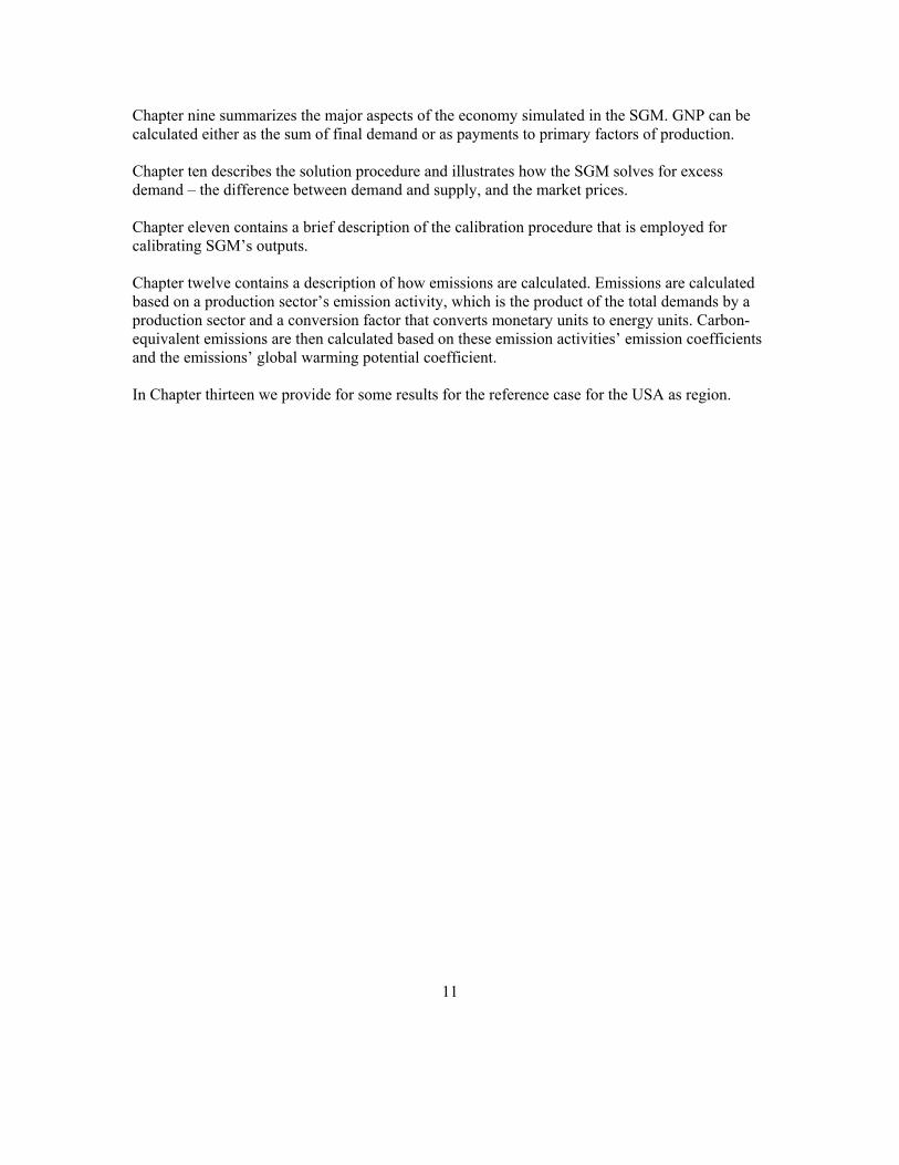
The flow of goods between industries and consumers in an economy can be described by means of an input-output table in value terms (see Figure 2), which maps directly onto Figure 1. An economic input-output table has three major sections: inter-industry flows, value added, and final demand. An input-output table is organized with inputs as rows and activities (production) as columns. Inputs include direct inputs and intermediate (inter-industry) inputs (those derived from a production process) and primary factors of production. The primary factors of production are rental of land, labor income, other value added, and indirect business taxes.7 Activities that use inputs are industries, and consumption by the final demand sectors: households, government, investments, and net exports (exports minus imports).

7 Indirect business taxes, less subsidies, are modeled as a proportional tax on production.

14

Production Activities Trade Inv Gov Hh

Intermediate Inputs

Primary Factors

Interindustry Flows

FinalDemand

Value Added

Figure 2 Typical input-output table

In the SGM, regional economic input-output tables are combined with regional energy balance tables to create regional hybrid input-output tables (see also Miller and Blair 1985). Economic input-output tables alone are not sufficient to determine the quantities of oil, gas, coal, electricity, and refined petroleum that are produced and consumed. Supplemental information on energy quantities is required to map monetary units from an input-output table to energy units needed to calculate levels of greenhouse gas emissions.

Energy Inputs

Production Imports Exports

Electricity Oil refining Coking

Agriculture Industry Transport

Sources

Energy

Final

Gas processing

Everything else (ETE)

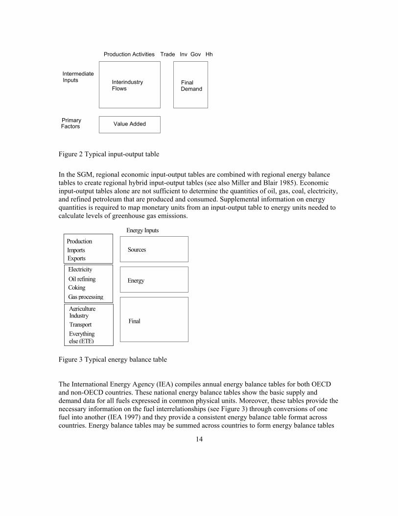
Figure 3 Typical energy balance table The International Energy Agency (IEA) compiles annual energy balance tables for both OECD and non-OECD countries. These national energy balance tables show the basic supply and demand data for all fuels expressed in common physical units. Moreover, these tables provide the necessary information on the fuel interrelationships (see Figure 3) through conversions of one fuel into another (IEA 1997) and they provide a consistent energy balance table format across countries. Energy balance tables may be summed across countries to form energy balance tables

15

for multi-country regions. The SGM uses IEA energy balances for all of the multi-country SGM regions, and uses local energy data for all of the following single-country regions, United States, Canada, Japan, China, India, Mexico, South Korea, and Brazil, given that the IEA energy balance tables are not as detailed as may be obtained from these local governments. Table 2 Production sectors and sub-sectors in SGM 2003

Sector SGM 2003

No. Sector / Markets Subsectors

Everything Else (ETE) 2 EveryThing Else sector 3 Crude oil production 4 Natural gas production

Energy Production

5 Coal production 9 Oil refining 10 Distributed gas production 6 Coke production

Oil (8.1) Gas (8.2) Coal (8.3) not active Nuclear (8.5)

Energy Transformation

8 Electricity generation

Hydro (8.6) 11 Paper and pulp 12 Chemicals 13 Cement 14 Primary metals 15 Non-ferrous metals

Industry or Manufacturing

16 Other industry and construction 17 Passenger transport Transportation 18 Freight transport 1 Other agriculture 19 Grains and oil crops 20 Animal products 21 Forestry

Agriculture

22 Food processing

Carbon 23 Carbon prices and/or GHG emissions 24 Land (Factor market) 25 Labor (Factor market) 26 Capital (Factor market) also called “other value added” or OVA

Economic input-output tables contain varying amounts of sectoral detail, depending on the country, with anywhere from 30 to over 500 producing sectors. The tables are aggregated to the level of detail that best matches the structure of SGM. Usually, an input-output table contains the same number of producing sectors as there are intermediate inputs. This does not have to be the case however because some industries may produce more than one product and some inputs might not be produced domestically and must be imported. The number of production sectors and markets simulated in the SGM is flexible. In the reference case, production sectors with markets are implemented for the so-called “Everything Else” sector or ETE, three energy production

16

sectors, four energy transformation sectors, five agriculture sectors, six industrial sectors, a passenger transport sector, a freight transport sector, and a carbon sector (see Table 2). Since the SGM is an energy model as well as an economic model, attention is paid to maintaining energy balances as the model operates through time. An energy balance table is used for base year calibration of energy production and consumption. Original units might be tons of coal equivalent (China), tons of oil equivalent (International Energy Agency statistics), or calories (Japan). The SGM uses joules for all energy units, expressed as either petajoules (PJ) or exajoules (EJ). The merging of an economic input-output table with an energy balance table presents a special problem: oil and natural gas are a joint product from a single industry in input-output tables, producing a single composite product. This is one area where energy balance tables provide essential information to maintain a clear distinction between oil and natural gas consumption.

The following steps are used to create a hybrid commodity-by-commodity input-output table from an economic input-output table and energy balance table (Sands 2002).

1. Put the economic input-output table in a format suitable for SGM. This involves aggregation across producing sectors and possible conversion to a 1990 base year.

2. Obtain 1990 energy balance table and convert units to joules. 3. Aggregate energy balance table across fuels to match the SGM format. 4. Rearrange activities (rows) within the energy balance table to match those of the

economic input-output table. 5. Transpose the energy balance table so that rows correspond to fuel inputs and columns

correspond to energy-consuming activities. 6. Create a hybrid input-output table where the energy rows (inputs) come from the

transposed energy balance table and all other rows come from the economic input output-table. This table is no longer in value terms but is now considered to be in quantity terms with units of joules for the energy rows and units of 1990 dollars (or other local currency) for all other rows.

7. Find a set of prices for all intermediate inputs that will rebalance the hybrid input-output table in value terms. By rebalancing, we mean that the value of output in each producing sector is equal to the total value of inputs. A linear equation may be derived for each producing sector, resulting in a system of equations that can be solved to obtain a price for each intermediate input8. It is important to note that these prices are derived from the calibration process and are not historical prices. This reflects the SGM modeling philosophy that assumes that technology characteristics, represented by the input-output and energy balance data, should determine relative prices in the model, and not the other way around.

8. Finally, create a new hybrid (economic and energy information) input-output table in value terms by multiplying all quantities by their respective prices (paid). The resulting

8 These linear equations are sometimes referred to as zero-profit conditions.

17

commodity-by-commodity table elements represent quantities expressed in 1990 million dollars.9

9. Units for the non-energy inputs in the hybrid input-output table are usually redefined so that prices equal one in the base year.

10. Thus, baseline information obtained consists of o the regional commodity-by-commodity hybrid input-output tables, including land,

and labor prices, information on capital for production sectors and taxes imposed (e.g., Appendix A)

o information on final demand sector supply and demands in the form of domestic consumption by households, domestic consumption by government, domestic investment, gross exports, and gross imports

o initial market prices are set to one (see Appendix A) o energy price-converters (EJ per million 1990 regional currency; see Appendix A).

The final hybrid input-output tables provide regional representations of the economy that are completely consistent with base year (1990 for SGM 2003) energy balances. Energy production and consumption for each fuel will exactly match the quantities in the base year energy balance table, and emissions can be calculated (Sands 2002). Production and input-output tables in the SGM Each region’s base year input consists of a commodity-by-commodity hybrid input-output table. Each column in the table represents a production process in the SGM, either represented by a constant-elasticity-of-substitution (CES) or a fixed-coefficient (Leontief) production function. Through changes over time in population and labor productivity, and through autonomous time trends governing the efficiency of inputs in production processes projections can be made and historical changes in GDP, fossil fuel consumption and electricity generation can be calibrated against. The hybrid commodity-by-commodity input-output table provides information on the use of produced commodities in the production of other commodities. These interdependencies are the basics in the computation of each production sector’s production function technical scale efficiency coefficients (Fisher-Vanden et al. 1993:6), along with value-added information in the form of land and labor prices, and capital and tax information. Calibration of the production function coefficients allows observations of benchmark years to be reproduced. When anticipated technological change is incorporated in these coefficients, the model produces long-term projections. Appendix A shows an complete example of the input-output elements Xi,j,jj,v for all input supplies (rows) and all production sectors (columns), including the electricity production subsectors, the carbon sector and all final demand sectors, where i indicates the row number of the input in the input-output table, j represents the column number or production sector in the input-output table, 9 Appendix A provides essential information about transforming energy units (Joules) into monetary values (1990 dollars).

18

jj represents the production subsector column in the input-output table, and v represents the actively operating vintaged capital (technology). The input-output table represents a one-year snapshot of the economy at time t; for the base year inputs v=t. Units are quantities in monetary values. The summed input values XSi,v (Equation 1) for each of the regions are shown in Table 2 of Appendix A, showing the different regions’ input breakdowns. Total production is the sum of the intermediate products that are produced in a production sector j of technology vintage v (XSj,v); this summed production is the gross production of a commodity j. When subsectors jj are simulated, as in electricity generation, commodity j is calculated as the sum over the subsectors (Equation 2).

∑ ∑= =

=

22

1j

n

1jjv,jj,j,iv,i XXS Eq. 1

v,jj,j,27i

26

1i

n

1jjv,jj,j,iv,j XXXS =

= =

+

= ∑ ∑ Eq. 2

where i indicates the row number of the input in the input-output table, j represents the column number or production sector in the input-output table, jj represents the production subsector column in the input-output table,

v represents the actively operating vintaged capital (technology), n is the number of active production subsectors where n ≤ jj, Xi,j,jj,v are the input-output table elements, which for the base year values are called Xi,j,jj,v in the documentation and when the model procedures are described are referred to as EDVi,j,jj,v (vintage v, production sector j, or subsector jj, and supply sector i, demands), and Xi=27,j,jj,v is the production sector or subsector indirect business tax; note that these are added only for the production sectors (j=1:22), and not for the final demand sectors (j=24:27). When equilibrium conditions exist, supplies (inputs) meet demands, and excess demand – the difference between demand and supply – equals zero for all markets. Besides input-output tables, key parameters needed are base year capital, elasticities of substitution for the production sectors, and income and price elasticities for the final demand sectors. Individual sector and subsector technologies are characterized by the annualized cost of providing an energy service. Thus, additional data needed to determine the annualized cost include in addition to capital cost, equipment lifetime, annual fuel requirements, the interest rate, and other annual maintenance and operating costs.

Investment and capital stocks The SGM operates in five-year time steps and keeps track of capital stocks in five-year vintages. At the end of each SGM time period, the model converts investment for each producing sector into capital stock, with the capital stock defined to be five-years’ worth of investment. Each

19

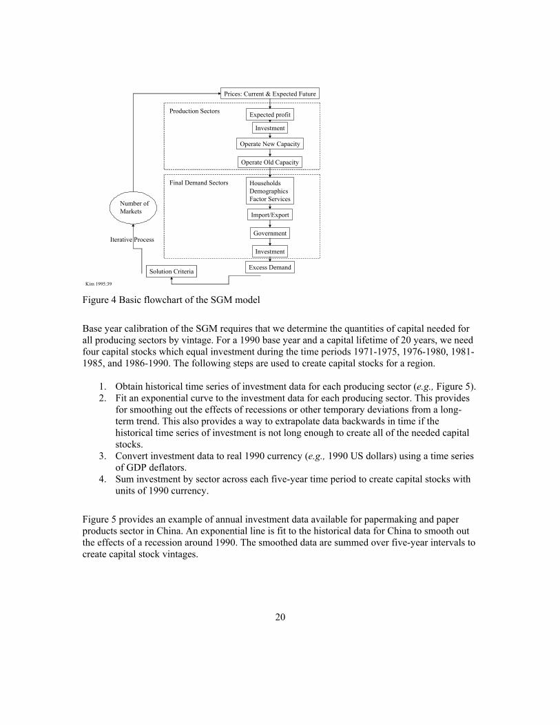
capital stock has a specified lifetime typically of four time periods or 20 years, the so-called nameplate lifetime of a technology10; the vintage indicator v of a technology keeps track of the operating technology capital stock’s age. Four vintages are operating simultaneously at each point in time, representing three operating old vintage technologies and one new technology that do differ in efficiency. Once capital is created it remains with its original sector, subsector and vintage until its planned retirement or when its profits are insufficient in meeting certain criteria. Vintage-specific capital stock is operated across its lifetime without change in technical efficiency. Thus, the SGM in effect operates as a hybrid commodity-by-commodity input-output table that gets solved by “clearing” its markets after supplies and demands are summed over its vintage-specific determination of supply and demand. In the SGM production of supplies and demands for consumption are determined separately, and the model has therefore has to reach equilibrium through a solution algorithm that adjusts market prices until excess demand ─ the difference between demand and supply, is less than the solution criteria, which is typically a small number (less than one but greater than zero). The solution algorithm needs only to access information on price, supply and demand to operate. SGM 2003’s solution algorithm first uses a bisection routine to bring individual markets closer to equilibrium and then uses a Newton-Raphson procedure for final convergence (see also Appendix B). Newton-Raphson relies on partial derivatives of supply and demand with respect to the unknown prices. Once the set of unknown prices is close to its final solution, Newton-Raphson converges very quickly. Prices adjusted by the iterative solution algorithm determine technology costs, demand for inputs, and sector outputs for a point in time. Old capital has limited ability to respond to changing prices; this is implemented by imposing short-run elasticities of substitution on the operation of old capital. New capital is assumed to be more flexible than old capital in its response to prices. Long-run elasticities of substitution, with values greater than short-run elasticities, allow for this greater flexibility. Long-run elasticities of substitution are imposed when investment decisions are made and when new capital is operated. Most production sectors use a single production function for each capital vintage. The electricity sector, however, is divided into subsectors that represent alternative processes for generating electricity such as gas-turbine, coal-steam, nuclear, or hydro. Market share within the electricity sector is based on expected the rate of return to new investments. Technologies with the highest expected rate of return receive the greatest market share. The major behavioral components of the SGM model thus describe the relationship between prices, production, and consumption of goods and services. Prices that are solved for are consistent with demands by producers and consumers for goods, services, and primary factors of production. Energy production and consumption balance, such that emissions can be accounted for. The behavioral components of the system are shown in Figure 4.

10 The modeler has the option changing any capital stock’s lifetime. The SGM has mostly been run with capital stocks lifetimes of 20 years.

20

Prices: Current & Expected Future

Expected profit

Investment

Operate New Capacity

Operate Old Capacity

Production Sectors

HouseholdsDemographicsFactor Services

Import/Export

Government

Investment

Final Demand Sectors

Excess DemandSolution Criteria

Number of Markets

Kim 1995:39

Iterative Process

Figure 4 Basic flowchart of the SGM model

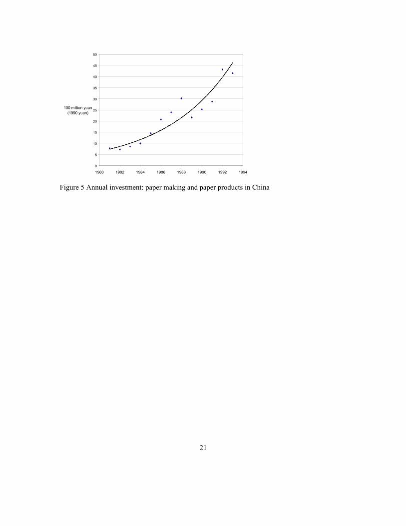
Base year calibration of the SGM requires that we determine the quantities of capital needed for all producing sectors by vintage. For a 1990 base year and a capital lifetime of 20 years, we need four capital stocks which equal investment during the time periods 1971-1975, 1976-1980, 1981-1985, and 1986-1990. The following steps are used to create capital stocks for a region.

1. Obtain historical time series of investment data for each producing sector (e.g., Figure 5). 2. Fit an exponential curve to the investment data for each producing sector. This provides

for smoothing out the effects of recessions or other temporary deviations from a long-term trend. This also provides a way to extrapolate data backwards in time if the historical time series of investment is not long enough to create all of the needed capital stocks.

3. Convert investment data to real 1990 currency (e.g., 1990 US dollars) using a time series of GDP deflators.

4. Sum investment by sector across each five-year time period to create capital stocks with units of 1990 currency.

Figure 5 provides an example of annual investment data available for papermaking and paper products sector in China. An exponential line is fit to the historical data for China to smooth out the effects of a recession around 1990. The smoothed data are summed over five-year intervals to create capital stock vintages.

21

0

5

10

15

20

25

30

35

40

45

50

1980 1982 1984 1986 1988 1990 1992 1994

100 million yuan(1990 yuan)

Figure 5 Annual investment: paper making and paper products in China

22

Chapter 3. Production functions A basic concept in the economic theory of production is the production function. A production function is a quantitative abstraction of a technology’s – or industry’s – productive operations. A typical industry transforms inputs (capital, labor, energy, materials, and land) into output. The production function relates the maximum output qj to any given vector of inputs xi: that is, qj=f(xi,t), where t is time, implying that the maximum output qj from a given set of inputs xi can change with time. Technological change can increase the maximum output. Natural resource exhaustion or environmental constraints can decrease the maximum output (Reister et al.). All goods in the SGM are produced with either a Constant-Elasticity-of-Substitution (CES) production function or a fixed-coefficient (Leontief) production function. These are constant-returns-to-scale production functions11; they are operated with one fixed input, capital in SGM 2003. Thus, among the key parameters needed for the SGM are elasticities of substitution for the production sectors.12 Oil refining is represented by a fixed-coefficient production function, as is electricity generation from its various energy sources, while most other production sectors are based on the CES production function. The production functions are described below. We describe in Chapter four “Prices and expected prices” and in Chapter five describe how operating vintages relate to the technical scale coefficients and elasticities. That information is required to understand the way in which the production functions relate to profits and demands as described in Chapter six. Production functions, vintages, and the input-output matrix The hybrid commodity-by-commodity input-output table, excluding the final demand sectors, provides representations of the inputs i (rows), to a production process in any sector j or subsector jj (columns). For each input there is an associated price and quantity. Each production process is tracked for its lifetime by vintage v; each vintage is the accumulated capital stock over 5 years of investment. Once capital is created, it must remain within its original sector or subsector and can be operated until its retirement. The primary advantage of this vintage structure is to better describe technical change over time and provide the option for putty-semiputty and putty-clay behavior in capital stock (Kim 1995:37) (putty for flexible; clay for fixed). Because capital stock cannot shift from one sector to another, new technologies affect productivity only at the margin; once a technology is installed, capital

11 “ ‘Returns to scale’ describes the output response to a proportionate increase of all inputs” (Henderson and Quandt 1971:79). 12 The elasticities of substitution for the reference case for the USA for the production sectors and the income and price elasticities for the final demand sectors can be found in Appendix A.

23

costs no longer matter. To operate or idle a technology depends solely on the ability of the technology to recover its current operating expenses plus taxes less subsidies. Vintaging is associated with the SGM’s five-year time steps (Nstep), that is, each vintage represents 5 years of investment. For the base year 1990, v equals zero, implicitly representing investments from 1986 through 1990, while older vintages are represented by negative integers. Vintage v=-1 represents investments from 1981 through 1985, etc. Table 2 illustrates the relationships between SGM’s four vintaged production sectors and subsectors that are operating and the 12 time steps the SGM executes after the base year13.

Table 3 Relationship between vintages (v) and times of operation (t)

Year

t= 0:12

↓

Operating new vintage (new vintage operates with long-run elasticities of substitution)

Operating old vintages (old vintages operate with short-run elasticities of substitution)

1990 0 at t=0 for v=0 at t=0 for v=-3. –2, -1 1995 1 at t=1 for v=1 at t=1 for v=-2, -1, 0 2000 2 at t=2 for v=2 at t=2 for v=1, 0, -1 2005 3 at t=3 for v=3 at t=3 for v=2, 1, 0 2010 4 at t=4 for v=4 at t=4 for v=3, 2, 1 2015 5 at t=5 for v=5 at t=5 for v=4, 3, 2 2020 6 at t=6 for v=6 at t=6 for v=5, 4, 3 2025 7 at t=7 for v=7 at t=7 for v=6, 5, 4 2030 8 at t=8 for v=8 at t=8 for v=7, 6, 5 2035 9 at t=9 for v=9 at t=9 for v=8, 7, 6 2040 10 at t=10 for v=10 at t=10 for v=9, 8, 7 2045 11 at t=11 for v=11 at t=11 for v=10, 9, 8 2050 12 at t=12 for v=12 at t=12 for v=11, 10, 9

CES production by vintage The Constant-Elasticity-of-Substitution (CES) production function is a well-behaved homogenous, generic function that enables minimum coding for a wide range of analysis (Kim 1995:37). The CES production function has a constant return to scale;14 that is, output response is proportional to an increase of all inputs. Total factor production is determined by a growth rate applied to the technical scale coefficient (α0,j,jj,v and αi,j,jj,v) of the CES production function, affecting all factor demands equi-proportionally.15

13 The model is structured such that nameplate lifetimes of various sizes can be input and additional vintages are simulated. 14 “If output increases by the same proportion, returns to scale are constant for the range of input combinations under consideration” Henderson and Quandt 1971:79. 15 “A production function which belongs to the CES class has 2 major characteristics:

(1) it is homogeneous of degree one, and (2) it has a constant elasticity of substitution.” Henderson and Quandt 1971:85

24

Sands (2002), Kim (1995) and Edmonds et al. (1993) formulate the CES production function16 in the SGM as follows:

ρρρ ααα

/11N

1iv,jj,j,26iv,jj,j,26iv,jj,j,iv,jj,j,iv,jj,j,0v,jj,j XXq

+= ∑

−

=== Eq. 3

where for each production sector j, or subsector jj and each operating vintage v,

qj,jj,v is the output or gross production of commodity j or jj produced by vintage v capital stock, which is stored in array PRDVj,jj,v in the SGM computer code and referred to as such in the documentation,

i is an indicator of an input to vintage v’s production of commodity j or jj, N is the total number17 of inputs i (26) in SGM 2003; if i equals 26, then i, in our case, refers

to the one fixed factor in the model, capital, N-1 is the number of variable inputs, α0,j,jj,v is a technical coefficient in vintage v’s production of commodity j reflecting the overall

production efficiencies of the vintages of production sectors j or jj, 0 indicator denotes that the parameter impacts the production sector as a whole (in this case

the technical scale coefficient α), αi,j,jj,v is an input-specific (i) technical scale coefficient in the production of commodity j or jj, αi=26,j,jj,v is the input-specific (i=26=capital) technical scale coefficient for capital (input N) in

the production of commodity j or jj,

The elasticity of substitution measures the rate at which substitution takes place. It is defined as the proportionate rate of change of the input ratio divided by the proportionate rate of change of technical substitution, where the rate of technical substitution is defined as –dx2/dx1 where x1 and x2 are inputs (Henderson and Quandt 1971:85-86; 62; 59). 16 Equation 3 is analogous to Edmonds et al.’s 1993 formulation:

ρρα

/1N

1iii0 )X(α)x(q

= ∑

= where ρ=(σ-1)/σ and σ=1/(1-ρ). See also Henderson and Quandt (1971:86: eq.3-35) and Chung (1994:111:eq.9.1). In the equations that follow, both ρ and µ are used as functions of σ: ρ = (σ-1)/σ and σ=1/(1-ρ) µ = (σ-1) = ρ/(1-ρ) and σ=(µ+1) -µ = ρ/(ρ-1) ρ/µ = 1/σ and µ/ρ = σ 1/ρ = σ/(σ-1) -1/ρ = -σ/(σ-1) = σ/(1-σ) 1/µ = 1/(σ-1) -1/µ = (ρ-1)/ρ = (-1/σ) • (σ/σ-1) = 1/(1-σ) 17 M is the number of primary factors; M=3 in this SGM version: capital (OVA, or KA; N=i=26), which is a fixed factor; and labor (N-1= i=25) and land (N-2=i=24), which are variable factors; the indirect business tax (IBT) associated with the production of commodity j or jj is the 27th i input (N+1=27).

25

Xi,j,jj,v is demand for input i in vintage v’s production of commodity j or jj; this demand is denoted by Xi,j,jj,v in the base year in the documentation and stored in array EDVi,j,jj,v in the SGM computer code and denoted as such in the documentation when not referring to the base year,

Xi=26,j,jj,v is the demand for the fixed (capital) input in vintage v’s production of commodity j or jj, and

ρ is a function of the elasticity of substitution parameter, σ, where ρ = (σ-1)/σ and σ=1/(1-ρ).

Long- and short-run elasticities The output of a CES production function is dependent on the elasticity of substitution, as shown in Equation 3 (see also Henderson and Quandt 1971: Chapter 3). In the SGM, when capital is operated as a CES production function, new capital operates under long-run elasticity, and all older vintages of capital operate under short-run elasticity. This means that new capital (new vintage) has a higher elasticity of technical substitution among inputs in response to changes in prices than old capital (old vintage). The type of technology simulated in the SGM in that case is so-called putty-semiputty technology.18 Sands (2002) summarizes how elasticities of substitution,σ, must satisfy the following relationship

10 newv,joldv,j <σ≤σ≤ == Eq. 4 where

old and new denote vintages, and j is the sector index

The model structure, with different elasticities of substitution between old and new capital, provides a way to simulate dynamics in marginal abatement curves, e.g., carbon prices must be driven higher in the short-run than in the long-run to meet any given carbon emission target. If the elasticity σ in the CES production function is specified to be less than 0.05, the SGM switches from a CES to a fixed-coefficient production function. The elasticity of substitution between inputs is then zero and the production function turns into a fixed-coefficient (or Leontief) technology. This switch in production functions is so called putty-clay technology. A graphical representation of a putty-semiputty technology, using CES production functions, is shown in Figure 6. Two isoquants are plotted, each with a different elasticity of substitution, sigma. An isoquant shows all combinations of two inputs that will produce one unit of output. An isoquant shows the physical tradeoffs available between these two inputs. For a given set of prices, only one point on the isoquant will minimize the cost of production. At that point, the

18 Putty-semiputty technology provides a lower elasticity of substitution in old capital than in new. Putty-clay technology assumes that new capital has a certain elasticity of substitution and that old capital is fixed-coefficient where the input-output coefficients do not respond to price. Putty-putty technology uses the same elasticity of substitution for both new and old capital.

26

isoquant is tangent to a line showing all combinations of equal expenditure on inputs. The slope of this line is the ratio of prices for the two inputs. A representative line of tangency is also shown.

σ = 0.5σ = 0.2

Input 1 →

↑ I n p u t 2

Figure 6 Putty-semiputty isoquants

During each SGM time period, new capital is formed. At the time of capital formation, the isoquant with the greater elasticity of substitution is used. However, at the end of the SGM time period, capital is converted from a higher to a lower elasticity of substitution. Once capital is constructed in SGM, substitution possibilities between inputs are limited. A putty-clay technology assumes that old capital is fixed-coefficient and the input-output coefficients do not respond to price. The input-output coefficients reflect relative prices that were in effect when the capital was new. Therefore, new capital is responsive to prices (putty), but input-output coefficients are locked into place as the capital is converted from new to old (clay). Isoquants for a putty-clay technology are shown in Figure 7.

σ = 0.5

σ = 0.0

Input 1→

↑ I n p u t 2

Figure 7 Putty-clay isoquants

27

The Leontief or fixed coefficient production function Some technologies are considered to be fixed-coefficient19 and have a Leontief functional form whether new or old, and their mix of input factors of production is not responsive to prices. This technology is referred to as clay-clay or simply clay. This assumption is sometimes used in the energy transformation sectors, especially oil refining, where the ratio of energy input to energy output is fixed in advance by physical processes and cannot respond to changes in price. All electricity subsectors are fixed coefficient. When a Leontief production function is implemented, an industry j or jj chooses the minimal amount of all intermediate and primary inputs i to produce output, leaving quantities of the inputs beyond the minimal amount idle (Chung 1994:170; Henderson and Quandt 1971:336). The Leontief production function can be described as follows:

=

v,jj,j,N

v,jj,j,N

v,jj,j,i

v,jj,j,i

v,jj,j,1

v,jj,j,1v,jj,j,0v,jj,j

X.....

X,,

Xminq

λλλλ K Eq. 5

where for each production sector j, or subsector jj and each operating vintage v,

qj,jj,v is the output or gross production of commodity j or jj produced with vintage v capital stock, later in the documentation denoted by PRDVj,jj,v,

i is the input to vintage v’s production of commodity j, N is the number of inputs i (N=26); if i equals 26, then i refers, in our case, to the one fixed

factor in the model, capital, λ0,j,jj,v is a technical scale coefficient in vintage v’s production of commodity j or jj reflecting

the overall production efficiencies of the vintages of production sectors j or jj, 0 indicator denotes that the parameter (in this case the technical scale coefficient λ) impacts

the production sector as a whole, λi,j,jj,v represents the technical scale coefficients, and Xi,j,jj,v is demand for input i in vintage v’s production of commodity j or jj; this demand is

denoted by Xi,j,jj,v in the base year and by EDVi,j,jj,v in the forecasts, where jj denotes a production subsector.

19 The elasticity of substitution (σ) in CES production functions has a practical lower bound of 0.05 in economic models such as SGM. Elasticities less than 0.05 result in numeric overflows or underflows in double-precision. Fixed-coefficient production functions in SGM have an elasticity of substitution of exactly zero. Therefore, there is a range of substitution elasticities between zero and 0.05 that the SGM can not simulate.

28

Chapter 4. Prices and expected prices The model must find a set of prices that is consistent with demands by producers and consumers for goods, services, and primary factors of production. In Chapter ten we detail the market price solution process, but here and in Chapters five through nine we describe the details of the costs of operating capital and the various aspects of demand simulated in the SGM.

Base year prices and initial future prices In the SGM 2003 model runs, the base year market prices are set to one (Pi,t=0=1), given that base year input is based on equilibrium and Walras’ Law20 guarantees that (1) if an equilibrium set of prices exists, any positive scalar multiple of each of those prices is also an equilibrium set of prices and (2) any commodity can be chosen as a numeraire,21 which in the SGM is the commodity of the Everything Else sector. Future prices are determined relative to the price of the Everything Else sector, for which market prices remain one in the projections. Initial, base year capital interest rates (i=26) equal 0.06; land rental prices (i=24) do not play a role in the example data set and prices are set to zero. When land plays a role in SGM, the initial market price of land rental, Pi=24=ls,t, is calculated based on the total land available as supply and land demand (i=24; see Equation 6).

hh27j,ls24i

ls24it,ls24i ED

XSP====

==== = Eq. 6

where XSi=24=ls is the summed (total) demand for supply of land in the base year and

EDi=24=ls,j=27=hh is the total demand for supply of land (see “Households”). Similarly, the initial market price for labor, Pi=25=lbs,t the cost of bying a year’s worth of one laboror’s time, i.e., the average annual wage of labor could be calculated (i=25; see Equation 7) and should deliver the same results as the input parameters listed for the reference case; thus, labor’s market rental price is not set to one.

hh27j,lbs25i

lbs25it,lbs25i ED

XSP====

==== = Eq. 7

where XSi=25=lbs is the total demand for supply of labor in the base year, and

EDi=25=lbs,j=27=hh is the total demand for supply of labor (see “Households”). 20 “If all the commodities in an economy are included in a comprehensive market model, the result will be a Walrasian type of general-equilibrium model, in which the excess demand for every commodity is considered a function of the prices of all the commodities in the economy” Chiang (1967:52). 21 Numeraire: “ A unit of account, or an expression of a standard of value. Money is a numeraire, by which different commodities can have values compared” (Pearce 1992); Oxford: Numeraire – good used as a standard value for other goods. The price of the numeraire is defined to be 1.

29

In the base year market prices equal one (Pi,t=1), with the exception of labor; market prices in the projections result from the market solution processing but can be set exogenously. The prices for crude oil, land rental and the Everything Else sector are set exogenously in the reference case; the gas market price is also set exogenously, assuming that they are set globally and not regionally as in the example carbon policy run to be discussed in Chapter thirteen. When market prices are set exogenously they retain their exogenously set value in the market solution process. For the base year, prices received for commodity j produced in a production sector are calculated from the difference between the total demand for i inputs minus the indirect business taxes paid (i=1:27=1:N+1), divided by the total demand for i inputs. Prices received for a production sector commodity j are identical for all subsectors jj.

∑

∑+

=

+

=+=

=

−= 1N

1iv,jj,j,i

1N

1iv,jj,j,1Niv,jj,j,i

0t,j

X

XXPr Eq. 8

where ∑Xi,j,jj,v is the summed over N+1 demands for inputs i in the production of commodity j or jj

(see Equation 2), which includes Xi=N+1,j,jj,v, the indirect business tax from the hybrid commodity-by-commodity input-output

table, which is a production sector- or subsector-specific input parameter which needs to be substracted.

Determining prices paid for supplies by producers, prices received for produced commodities, and policy potential For a closed economy, the price paid by producers for supplies at each point in time includes transportation costs, taxes and adjustments. Prices paid for the variable inputs (i=1:23) from the ith supply sector for each of the actively producing vintages v for sectors j=1:22 and subsectors jj=1:6 at time t are calculated as follows:

( )ijj,j,ijj,j,iit,it,jj,j,it,jj,j,i CpfTxaddTxproImExPadjPi ++•••= Eq. 9 where

adji,j,jj,t, is a time-period-dependent adjustment factor that reflects markups and intra-regional transport costs; these adjustment factors can be input i and sector j or subsector jj specific; adji,j,jj,t is further described in Equation 11,

Pi,t is the market price; in the base year Pi,t equals one; in the forecasts Pi,t is calculated during the model solution process and is supply and demand dependent,

ExImi is a transportation cost multiplier, a rate parameter, Txproi,j,jj is a proportional tax rate on the ith product, Txaddi,j,jj is an additive tax on the ith product, and

30

Cpfi, is a carbon permit fee on inputs, i, per dollar of production based on the global warming potential and the emission coefficient of a fuel; thus

∑ ••••= =fn

fnifnregiont,23ii GWPPRconvrtEMCExchRatePCpf Eq. 10

where fn stands for oil, gas, or coal within a production process for which the energy supply

carbon fee is calculated, Pi=23,t is the carbon price, which, dependent on if and which carbon policy is implemented

may equal the market price during the model solution process, or may be fixed, ExchRateregion the monetary exchange rate, EMCfn is the fuel-specific carbon content in million tons C per exajoule of the energy

source; fn stands for oil, gas, or coal within a production process for which the energy supply carbon fee is calculated,

GWPfn is the global warming potential; GWPfn=1 for carbon, PRconvrti is the energy conversion factor, converting the relative prices in monetary units

to physical energy units. Note that PRconvrt for each supply sector in each region is expressed in energy units produced (EJ) per million 1990 regional currency (that is, per gross production of a commodity j, which is the sum of all intermediate products in the base year in 1990 million regional currency). Also note that the final conversion factors are the results of base year calibration. A time-dependent adjustment factor, adji,j,jj,t, reflects markups and intra-regional transport costs; these adjustment factors can be input i and sector j or subsector jj specific. A (sub)sector-specific price adjustment factor is calculated as a time-dependent interpolation of initial and terminal values when T as number of time periods t times the time step of five years (Nstep) is smaller than Tadjzi:

jj,j,ijj,j,i

jj,j,ijj,j,it,jj,j,i Tadjz

TAdjz)Tadjz

T1(Adadj •+−•= Eq. 11

where Adi,j,jj, Tadjzi,j,jj, and Adjzi,j,jj are input parameters and T is the number of time periods

multiplied with the time step (t*Nstep). In most cases adj equals one. However, adj is included in the equation calculating the price paid by the producer for inputs (Equation 9) to provide the model with increased flexibility in describing the purchase price.

The proportional tax, Txpro, and additive tax, Txadd, can be input and (sub)sector specific; they are presently only supply-price-specific, however. By changing the different rates in the above price-paid equation, researchers can evaluate policy scenarios. For example, carbon prices and energy excess fees can be imposed in the model by

31

changing Txadd or applying a carbon fee Cpf on the appropriate products whether they are fossil fuels or energy services. Technology specific discount rates Pii=capital,j,jj,t may be adjusted over time as follows:

26it,jj,j,capitalit,jj,j,capitali PwedgePi === += Eq. 12 The wedge component of the technology specific discount rate can be considered an interest rate wedge or discount rate. They can be calculated in the base year in a spreadsheet model for each of the sectors and subsectors. A target profit rate for each (sub)sector is calculated based on

o all active capital (KA), and o an expected profit rate weighed against zero profit by the sector where the expected profit

rate calculations are based on the CES production function and long-run elasticity, σ, and inputs from the IO table, which are based on base year information

The wedge component of the technology specific discount rate can be modified over time as part of the calibration process (see also Chapter eleven). Calculation of prices received (Prj,t) for the production sector-specific commodities produced, in relation to the market prices (Pi,t), are first steps in the model evaluation, since they determine operational and investment decision-making. Prices received for a production sector commodity are identical for all subsectors. For the projections they are calculated as follows:

j

jt,jt,it,j TxIBT1

ImExTrPPr

+

•+= Eq. 13

where Pi,t are the market prices which are updated during the model solution processing and are

therefore time-period-specific, ExImj is the transportation cost rate parameter (these input parameters equal one in the

reference case), TxIBTj is the production sector indirect business tax; these input parameters are constant over

time in the reference case, and Trj,t is a time-period-dependent transportation cost factor.

The region-specific transportation cost factors are calculated as time-dependent interpolations of initial and terminal values as long as T, which is the number of time periods multiplied by the time step (T=t*Nstep, where Nstep equals 5 years), is smaller than Trzi.

jj

jjt,j Ttrz

TTrz)Ttrz

T1(TriTr •+−•= Eq. 14

where Trij, Ttrzj, and Trzj are input parameters.

32

The equations above are cycled through each row i and column j and jj element of the input-output matrix, and each of the vintage-specific Pii,j,jj,t matrices are filled for each element of the matrix at each point in time for each of the operating vintages. The model is solved after summing the vintage-specific inputs to production and vintage-specific calculated demands. Note that prices for input to production are identical for all operating vintages and will be only differentiated among production sectors by the adjustment factors adji,j,jj,t that reflect markups and intra-regional transport costs, the proportional tax rates Txproi,j,jj and the additive taxes Txaddi,j,jj.

Expected prices The simplest rule for projected future prices is to set them equal to current prices. Alternatively, projected future prices can be based on a previous model run. A third option is to determine expected prices as projected future prices discounted to the present. In the SGM expected future prices for all variable inputs (i=1:25) are calculated such that investment decisions based on expected profitability can be made. The expected prices paid Piei,j,jj (i=1:25) for the next point in time are calculated based on prices paid by producers for inputs (see Equation 9). These prices are production sector- and production subsector-specific.22

( ) ( )

+−•

+•

+•=

===

expT

t,jj,j,26it,jj,j,26i

5.0

t,jj,j,26it,jj,j,ijj,j,i Pi1

11Pi

11)Pi1

1PiPie Eq. 15

Expected prices received for the commodities produced by the production sectors and subsectors are based on the prices paid for inputs (see Equation 9) and the prices received for commodities produced (see Equation 13).

( ) ( )

+−•

+•

+•=

===

expT

t,jj,j,26it,jj,j,26i

5.0

t,jj,j,26it,jjj,j,i Pi1

11Pi

11)Pi1

1PrPe Eq. 16

where Pii,j,jj,t is the prices paid by the producer for supplies (see Equation 9), Prj,t is the price received for a commodity produced (see Equation 13), Pii=26,j,jj,t is the interest rate, which is production sector- and subsector-specific (Equation 12), Texp is the nominal life of the investment (years) and a parameter of technology, and

22 Note that the equations as described here are easily solved analytical equations and replace the original equation that had to be solved iteratively (eq. 15 in Edmonds et al. 1993). The original equations were described as follows: Pej, for time t is calculated as discounted price for product j (either an input or an output) by

tj

expT

1t0t,jt,j )dis1(

r1)t(P)T(Pe

+

+•= ∑

= where Texp is the nominal life of the investment; rj is the rate of expected price change; and dis is the discount rate. The nominal life of the investment is a parameter of the technology. This parameter value may be different from the maximum potential life of the technology. Both the rate of expected price change rj and the discount rate dis are behavioral variables.

33

Texp equals t•Nstep, where t is the number of time-step periods the investment is operational; thus Texp=20 when t=4, given that SGM’s timestep (Nstep) equals five years. The difference between the expected prices for input supplies Piei,j,jj and the expected prices for the output products Pej,jj is thus based on the difference between the price paid for input Pii,j,jj,t and the price received for a commodity j produced Prj,t at time t.

34

Chapter 5. Technical change Technology is a central feature shaping anthropogenic greenhouse emissions. Given that technology is “the broad set of processes covering know-how, experience and equipment, used by humans to produce services and transform resources” (Edmonds and Moreira, 2004), technology is a central issue in understanding climate change. Technology unifies the elements of the system. Technology shapes many elements of SGM design. This chapter describes how technical change is implemented in the SGM. In brief, technical change is imposed on the scale coefficients of the input-output table that relate the supply sectors to the production sectors. In addition, we describe how autonomous efficiency improvements are imposed on energy use in households and the government and the changes over time. Input-output coefficients and their relationship to the technical scale coefficients The SGM keeps track of capital stocks in five-year vintages. Vintage-specific capital stock is operated across its lifetime without change in technical efficiency. The four vintages operating simultaneously at each point in time represent three old vintage technologies and one new technology. Old and new vintages may be characterized by different elasticities (denoted by “σ”) of substitution given that new capital can be expected to be more flexible than old capital and its elasticity of substitution will therefore be greater than or equal to the corresponding elasticity of substitution for old capital. The SGM’s framework is a hybrid commodity-by-commodity input-output table in monetary values where for energy the input-output dollar values remain related to the per-joule cost of energy. The relationship between input-output coefficients (denoted by “a”) and the technical scale coefficients (denoted with “α” for a CES production function and with “λ” for a Leontief or fixed-coefficient production function) that are implicit in an input-output table was described by Sands (2000) and can be summarized as follows. The physical input-output coefficients can be derived from a hybrid input-output table for each combination of input and production processes. An input-output coefficient is the quantity of input divided by the quantity of output. The quantity of output is found by dividing the value of output by its price. Similarly, the quantity of input is found by dividing the value of input by its price. In the special case of fixed-coefficient production, the technical coefficients of the production function are related to input-output coefficients in a very simple way which is independent of price:

j,0

j,ij,ia

λλ

= Eq. 17

where λ0,j are production sector-specific technical coefficients,

35

λi,j are technical coefficients that can incorporate technology-specific (i.e., non-neutral) technical change parameters. In general though, input-output coefficients are related to the technical coefficients of production functions through prices. The production process should substitute away from inputs that become relatively more expensive. The rate at which one input is substituted for another, relative to the rate of change in prices of those inputs, is accomplished through the implementation of the elasticity of substitution among inputs in production. In a constant-elasticity-of-substitution (CES) production function, this elasticity of substitution remains constant across changes in price. Equation 18 shows the dependence of input-output coefficients on CES technical coefficients, relative prices, and the assumed elasticity of substitution. In the SGM we invert this relationship and solve for technical coefficients as a function of input-output coefficients, prices, and the elasticity of substitution.

[ ])1/(1

i

j)1/(j,ij,0j,i p

p)p(a

−−

••=

ρρραα Eq. 18

where

ai,j is the amount of input i required per unit of output j; ai,j is called the input-output coefficient when dealing with input-output matrices,

α0,j is a production sector-specific technical coefficient that can incorporate a Hick’s neutral technical change parameter23

αi,j is a technology-specific technical coefficient that can incorporate a technology-specific (i.e., non-neutral) technical change parameter,

ρ is a function of the substitution elasticity; ρ=(σ-1)/ σ, where σ is a production sector-specific elasticity of substitution,

pj is the price received for the commodity produced, and pi is the price paid by the producer for input.

Note that the above equation uses subscripts for inputs and outputs, except for the exponent. This exponent actually does vary by producing sector as described above. As the SGM searches for equilibrium prices, technical coefficients remain invariant with respect to price. However, input-output coefficients will respond to changes in price. This response, governed by the elasticity of substitution is important for climate policy since changes in fossil fuel prices are an important component of the change in emissions. Note that the input-output table tells us nothing about the elasticity of substitution among inputs in production. That parameter must be set exogenously using published results from econometric studies, simulations of bottom-up technology models, or expert judgment.

23 Hick’s neutral technical change parameter reflects the overall production efficiency of a vintage (Fisher-Vanden 1993:12).

36

The SGM contains a large set of parameters that can be used to simulate technical change over time for any given production sector. Separate parameters are available for each input to each production process (and each vintage)24. The rates of change in input efficiency can be varied at each five-year time step in the SGM. For example, we could assume that energy efficiency in coal-fired electric generating plants is improving at a rate of 0.5% per year for 10 years, with no change after that. These technical change parameters are very powerful in determining energy consumption and emissions in a reference case, the impact of which is similar to the Autonomous Energy Efficiency Improvement (AEEI) that is used in some other energy models. In the SGM, exogenous rates of technical change can be specified for all inputs to production, not just energy. In the case of Hick’s neutral technological change, all of the α or technical scale coefficients (the parameters that relate the inputs to the production processes) within a production function are assumed to change at the same rate. Isoquants for the case of two inputs with neutral technical change are shown in Figure 8. Note that as technology improves from T0 to T2, the isoquant moves inward toward the origin, showing that less of each input is required to produce one unit of output.

Τ0

Τ1

Τ2

Input 1 →

↑ I n p u t 2

Figure 8 Neutral technical change when the elasticity of substitution coefficient (σ) equals 0.5

Instead of adjusting α0 to represent technical change, each of the αι,j parameters can be adjusted with its own technical change parameters. If the rate of change in efficiency varies across inputs, then technical change is said to be non-neutral or biased. Figure 9 provides an example of biased technical change, with the isoquant shifting in towards the origin, but at different rates for different inputs. For example, we could have a technology for which labor productivity is improving at a faster rate than energy efficiency. In this case the amount of labor needed per unit of output is falling faster than the amount of energy needed per unit of output.

24 The technical scale coefficients remain constant over the lifetime of the vintage, while they differ among vintages.

37

Τ0

Τ1

Τ2

Labor →

↑ E n e r g y

Figure 9 Biased technical change when the elasticity of substitution coefficient (σ) equals 0.5

If the production process is fixed-coefficient, then these technical change parameters λ can be used to precisely control input efficiency. However, most production processes are not fixed-coefficient, at least in the long run as old capital is replaced by new capital. Most production processes respond to changes in prices of inputs by substituting away from those inputs that are relatively expensive. In this case, input efficiency is affected by both the exogenous technical change parameters described in this section and by changes in relative prices. Changes in input efficiency are a combination of exogenous technical change and price-induced technical change.25 Exogenous technical change is represented by a shifting isoquant; price-induced technical change is represented by shifts along an isoquant. Besides production efficiency, there are parameters that determine land, labor, and capital productivity. Labor productivity parameters are the primary determinants of economic growth in SGM and are used to influence the time path of GDP in a reference case. Both energy efficiency and labor productivity assist in constructing reference scenarios. The labor productivity parameters are used to determine a time path for GDP and the energy efficiency parameters are used to determine consumption efficiency of energy by fuel (see also Chapter eleven).

How technical change is operationalized in the SGM For each region technical change parameters for each sector j, each subsector jj, and each time period t determine the efficiency improvements in energy production, energy transformation (e.g., oil refining, gas processing, coal and electricity generation), industry, transportation and agriculture, and the efficiency of labor productivity, land productivity, and capital. The TECHNN parameters or γ parameters are set to identical values for all industries, while coal production, gas production and distribution, oil refining and electricity production have their 25 Note that the SGM does not attempt to simulate induced technical change. In that case, an isoquant would shift inward in response to a change in prices or some other policy signal, perhaps with a time lag.

38

unique efficiency parameters (see Appendix A for example values). Technical change over time is calculated as a multiplier called Factor of the technical scale coefficients α for the CES formulation and λ for the Leontief formulation.

Nstep1t,jj,j,it,jj,j,i )TECHNN1(FactorFactor +•= − (unitless) Eq. 19

where

Nstep is the time step of 5 years, t denotes the number of 5 year time steps since the base year; in the base year t=0, Parmname (TECHNN or γ) indicates the sector-, or subsector-dependent regional technology-

dependent technological rate change (unitless). Technical change parameters are also implemented for household and government fuel use such that improved energy-use efficiency can be simulated.

Household (j=hh) fuel-use changes over time are calculated by means of the following factor, the implementation of which is discussed under “Household Demands”:

Nstephh,it,hh,i )HHAEEI1(Factor += (unitless) Eq. 20

where

HHAEEIi,hh is a technical change parameter for household fuel use. Government (j=gv) fuel-use changes over time are calculated by means of a similar calculation:

Nstepgv,it,gv,i )GVAEEI1(Factor += (unitless) Eq. 21

where GVAEEIi,gv is a technical change parameter for government fuel use.

Implementation of the government fuel use factor is discussed under “Government Demands.” Technical change as described above is implemented in exactly the same way for all production functions in the SGM. Thus, Factor is used as a multiplier of a technical coefficient such that a change over time in technology is simulated.

The technical coefficients (αi,j) in the CES production function The technical scale coefficients (αi,j) are extracted from CES production functions for the base year as follows:

t,ETEi

t,i

t,ETEiv,jj,j,ETEi

t,iv,jj,j,iv,jj,j,i P

PP/XP/X

=

µρ

==

•

=α Eq. 22

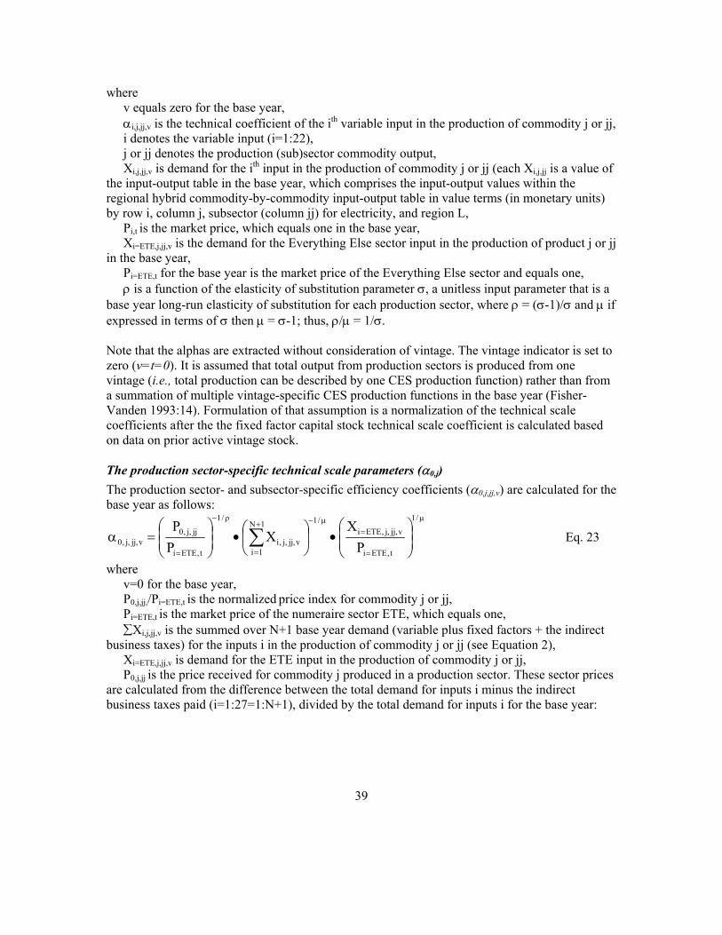
39

where v equals zero for the base year,

αi,j,jj,v is the technical coefficient of the ith variable input in the production of commodity j or jj, i denotes the variable input (i=1:22),

j or jj denotes the production (sub)sector commodity output, Xi,j,jj,v is demand for the ith input in the production of commodity j or jj (each Xi,j,jj is a value of the input-output table in the base year, which comprises the input-output values within the regional hybrid commodity-by-commodity input-output table in value terms (in monetary units) by row i, column j, subsector (column jj) for electricity, and region L,

Pi,t is the market price, which equals one in the base year, Xi=ETE,j,jj,v is the demand for the Everything Else sector input in the production of product j or jj in the base year,

Pi=ETE,t for the base year is the market price of the Everything Else sector and equals one, ρ is a function of the elasticity of substitution parameter σ, a unitless input parameter that is a

base year long-run elasticity of substitution for each production sector, where ρ = (σ-1)/σ and µ if expressed in terms of σ then µ = σ-1; thus, ρ/µ = 1/σ. Note that the alphas are extracted without consideration of vintage. The vintage indicator is set to zero (v=t=0). It is assumed that total output from production sectors is produced from one vintage (i.e., total production can be described by one CES production function) rather than from a summation of multiple vintage-specific CES production functions in the base year (Fisher-Vanden 1993:14). Formulation of that assumption is a normalization of the technical scale coefficients after the the fixed factor capital stock technical scale coefficient is calculated based on data on prior active vintage stock.

The production sector-specific technical scale parameters (α0,j) The production sector- and subsector-specific efficiency coefficients (α0,j,jj,v) are calculated for the base year as follows:

µ

=

=µ−+

=

ρ−

=

•

•

=α ∑

/1

t,ETEi

v,jj,j,ETEi/11N

1iv,jj,j,i

/1

t,ETEi

jj,j,0v,jj,j,0 P

XX

PP

Eq. 23

where v=0 for the base year,

P0,j,jj,/Pi=ETE,t is the normalized price index for commodity j or jj, Pi=ETE,t is the market price of the numeraire sector ETE, which equals one, ∑Xi,j,jj,v is the summed over N+1 base year demand (variable plus fixed factors + the indirect

business taxes) for the inputs i in the production of commodity j or jj (see Equation 2), Xi=ETE,j,jj,v is demand for the ETE input in the production of commodity j or jj,

P0,j,jj is the price received for commodity j produced in a production sector. These sector prices are calculated from the difference between the total demand for inputs i minus the indirect business taxes paid (i=1:27=1:N+1), divided by the total demand for inputs i for the base year:

40

∑

∑+

=

+

=+=−

= 1N

1iv,jj,j,i

1N

1iv,jj,j,1Niv,jj,j,i

jj,j,0

X

XXP Eq. 24

where v=0 for the base year,

∑Xi,j,jj,v is the summed over N+1 demands for the inputs i in the production of commodity j or jj (see Equation 2) in the base year, which includes

Xi=N+1,j,jj,v, the indirect business tax from the hybrid commodity-by-commodity input-output table, which is a production sector- or subsector-specific input parameter which needs to be substracted.

The fixed-factor-specific scale coefficients for capital stock (αi=N=capital stock,j ) The fixed-factor-specific scale coefficients for capital stock (αi=26=capital,j,jj,v ) for each production sector j and subsector jj for the base year are calculated in steps and are a direct result of SGM’s profit-making assumption:

v,jj,j0

3vv,jj,j

v,jj,j,0

1N

1iv,jj,j,i

v,jj,j,26i ZKAprior

1X

•

•α

=α

ρ

−=

+

==

∑

∑ Eq. 25

where ∑Xi,j,jj,v is the summed demand for the inputs i in the production of commodity j or jj in the

base year and v equals zero for the base year, KApriorj,jj,v is the vintage capital stocks that is active prior to the base year 1990, and

Zj,jj,v is calculated as follows for the base year when no or zero profit expectations are incorporated:

∑−

= =

µ

αα

••α−=1N

1i v,jj,j,ETEi

v,jj,j,it,ijj,j,0v,jj,j,0v,jj,j P)P(1Z Eq. 26

where v equals zero in the base year,

P0,j,jj is the price received for commodity j or jj in the base year (see Equation 24), α0,j,jj,v reflects the overall production efficiency of the vintage, Pi,t is the market price, which equals one in the base year, αi,j,jj,v is a technical scale coefficient of the ith input (supply) in(to) the production of

commodity j or jj, αi=ETE,j,jj,v is the technical scale coefficient of the numeraire sector.

Normalizing the alphas (αi,j where i=0:26 and j=1:22) For normalization of the alphas, all alphas (i=0:26; N=26) are summed, including α0,j,jj,v and αi=26=capital,,j,jj,v and each of the alphas is recalculated by dividing by this sum:

41

∑=

=

α

α=α 26N

0iv,jj,j,i

v,jj,j,iv,jj,j,i for i=1:26 and j=1:22 Eq. 27

The production sector-specific efficiency parameters, α0,j,jj,v, are re-calculated as follows:

ρ

=

=

α

α=α

∑

/1

26N

0iv,jj,j,i

v,jj,j,0v,jj,j,0 Eq. 28

The vintage alphas and incorporation of technical change The vintage alphas are calculated in three steps: (1) First, assumed future technical change is incorporated. All alphas (i=0:26; j=1:22; jj=1:6), from the oldest vintage (v=-3) through the time zero vintage (v=t=0), αi,j,jj,v=-3:0, are set equal to αi,j,jj,v=0, which are calculated as shown above (Equations 22 through 27) and all alphas for the variable factors and for capital stock are projected into the future (t=1:12) as follows:

ραα t,jj,j,i1v,jj,j,iv,jj,j,i Factor•= − Eq. 29

where v equals t-3:t,

αi,j,jj,v-1, the previous vintage-active alpha, is updated for each time period by implementing the technological change assumptions:

Nstepjj,j,i1t,jj,j,it,jj,j,i )Tech1(FactorFactor +•= − (see Equation 19)

where Nstep is the time step of 5 years, and Techi,j,jj is the production sector-dependent regional technology-dependent technological

rate change, which for αi,j,jj,v is referred to as Parmname, and ρ is a function of the production sector-specific long-run elasticity σ.

Note that Factori,j,jj,t=1 in the base year when t=0. (2) Second, the overall production efficiency, α0,j,jj,v , is incorporated into the alphas. These transformed alphas – by region, sector, subsector, input, and vintage, including the capital stock (i=26) – are calculated as follows:

v,jj,j,iv,jj,j,0v,jj,j,i ααα ρ •= Eq. 30

( ) )1/(1v,jj,j,iv,jj,j,icst ρ−α=α Eq. 31

42

where ρ is a function of the long-run elasticity of substitution and equals (σ-1)/σ. (3) Third, the alpha0s (α0,j,jj,v) for all production (sub)sectors (j and jj), all vintages (v) and time periods are set to one after being “used” in the equation above. This allows alpha0 to be used for energy supply calibration.

1v,jj,j,0 =α Eq. 32 and

1cst v,jj,j,0v,jj,j,0 == •ρσαα Eq. 33 Imposing changes in elasticities of substitution When capital becomes “old vintage” the technical coefficients’ long-run elasticity σ1 of substitution is converted to short-run elasticity σ2 and profit rate is included:

)11/()21(

v,jj,jv,jj,j

t,j)11/()21(v,jj,j,26iv,jj,j,26i KA

Prρ−ρ−ρ

ρ−ρ−==

π•α=α Eq. 34

where v=t-3:t,

αi=26=capital,j,jj,v was normalized (in Equation 27 based on Equation 25), ρ1 is a function of the long-run substitution elasticity [(σ1-1)/ σ1], and ρ2 is a function of the short-run substitution elasticity [(σ2-1)/ σ2], Prj,t is the price received for commodity j (see Equation 13 in the “Price and expected price”

section) at time t, πj,jj,v / KAj,jj,v is the vintage-specific production (sub)sector profit rate ─ that is the profit

relative to capital cost, or annual return per dollar of invested capital ─ for which the calculations are described in Chapter six, and KAj,jj,v is the vintage-specific production sector or subsector capital stock; for the base year KAj,jj,v=KApriorj,jj,v and in the projections KAj,jj,v is set equal to the linearly interpolated annual capital investment flow over a five-year period (from the current point in time back to the previous model solution-point in time [see Equation 118]).

v,jj,jv,jj,j KApriorKA = Eq. 35 The vintaged-specific production sector or subsector-specific technical scale coefficients (for i=1:25 and j=1:22; for jj=1:6 if active) for old vintages are calculated as follows:

)11/()21(

t,jj,j,i

t,j)11/()21(v,jj,j,iv,jj,j,i Pi

Prρ−ρ−ρ

ρ−ρ−

•α=α Eq. 36

where v equals t-3:t,

43

αi,j,jj,v, is based on the calculation in Equation 28, Pii,j,jj,t are the prices paid by the producer for supplies (see Equation 9), Prj,t is the price received for a commodity produced (see Equation 13).

All alphas, including alpha for capital interest (i=26) are then once more transformed before being used in the calculations when operating old vintages (see “Profits, demands, expected profit rates, and the operation of capital”).

( ) )21/(1v,jj,j,iv,jj,j,icst ρ−α=α Eq. 37

where v equals t-3:t,

α0,j,jj,v equals one, αi,j,jj,v is based on its last transformation in Equations 34 for capital costs and in Equation 36

for the variable factors, and σ2 is the short-run elasticity of substitution, which can also be expressed as

1/(1-ρ2) and

1cst 22v,j,0v,j,0 == •ρσαα Eq. 38

where ρ2 is a function of the short-run substitution elasticity [ρ2=(σ2-1)/ σ2].

Note that after the transformation processes the adjusted α0,j,v for each production sector is set to one. The technical coefficients (λi,j) in the Leontief production function For potential substitution of each of the production functions’ technical coefficients based on the CES production function (α0,j,jj,v; αi,j,jj,v; αi=26=capital,j,jj,v) by technical coefficients based on the fixed coefficient or Leontief production function (λ0,j,jj,v; λi,j,jj,v; λi=26=capital,j,jj,v), the Leontief technical coefficients are calculated. These Leontiefs are, as are the alphas, calculated from the hybrid commodity-by-commodity input-output table values and prices. Base year computations are given in Equations 39-32, projections in Equation 43. For the base year the technical coefficients for the Leontief production function (λi,,j,jj,v for i=1:25 and j=1:22 and jj=1:6 when active) are computed as follows:

∑=

=

==λ N

1i0t,jv,jj,j,i

0t,jj,j,iv,jj,j,iv,jj,j,i

Pr/X

Pi/X Eq. 39

where v=0 for the base year,

N equals the variable plus fixed factors,

44

Xi,j,jj is base year demand for the ith input in the production of commodity j or jj (each Xi,j,jj is a value within the regional hybrid commodity-by-commodity input-output table),

∑Xi,j,jj,v is the summed base year demand for the inputs i in the production of commodity j or jj,

Pii,j,jj,t are the prices paid by the producer for supplies (see Equation 9), and Prj,t is the price received for a commodity produced (see Equation 13).

For the base year the production sector-specific efficiency coefficients for the Leontief production function λ0,j,jj,v are set to one.

1v,jj,j,0 =λ Eq. 40 The capital cost technical scale coefficients (i=26) for the base year are calculated as follows:

∑

∑

=

−=== =λ N

1it,jv,jj,j,i

0

3vv,jj,j

v,jj,j,capital26i

Pr/X

KAprior Eq. 41

where KApriorj,jj,v is the capital stock vintage that is active for a production sector in the base year, ∑Xi,j,jj,v is the summed base year demand for the inputs in the production of commodity j in the

base year, Prj,t is the price received for commodity j at time t.

Note that the vintaged and projected technical coefficients λ are only calculated when the elasticity of substitution for the production sector equals or is smaller than 0.05. Note that these elasticities are inputs for each production sector (for an example, see Appendix A). Vintaged production sector or subsector-specific efficiency coefficients λ0,j,jj,v for a Leontief production function are always set to one in the reference case.

1v,jj,j,0 =λ Eq. 42 Implementation of technical change is formulated as follows:

Nstepi

1t,jj,j,it,jj,j,i )1( γ+

λ=λ − Eq. 43

thus, with large values of γi, λij gets smaller and demand decreases, or differently put, supplies are used more efficiently. For the technical coefficient of capital any value besides zero, of γi will result in more costly capital over time.

45

In the case of putty-clay behavior a sector’s vintaged and projected technical coefficients for the Leontief production function (λi,,j,jj,v for i=1:25 and j=1:22) are based on the vintage technical coefficients calculated for the CES production function.

)1/(1

t,jj,j,i

t,jv,jj,j,i

)11/(1v,jj,j,0v,jj,j,i Pi

Prρ−

ρ−ρ

•α•α=λ Eq. 44

where α0,j,v equals one, ρ1 is a function of the long-run elasticity σ1 which equals less or equal 0.05, αi,j,jj,v is based on long-run elasticity and has technological change incorporated, Pii,j,jj,t are the prices paid by the producer for supplies (see Equation 9), and Prj,t is the price received for a commodity produced (see Equation 13).

And the Leontief vintaged and projected technical coefficients for capital are then also based on the vintage technical coefficients calculated for the CES production and on the profit rate:

)11/(1

v,jj,jv,jj,j

t,jv,jj,j,26i

)11/(1v,jj,j,0v,jj,j,capital26i Ka/

Pr ρ−

=ρ−ρ

==

π•α•α=λ Eq. 45

where α0,j,jj,v equals one, αi=26=capital,j,jj,v will be based on long-run elasticity and has technical change incorporated, Prj,t is the price received for the commodity j produced at time t, Kaj,jj,v is the capital stock vintage that is active, πj,jj,v are profits for which the calculations are described in “Profits, demands, expected profit

rates, and the operation of capital.”

46

Chapter 6. Profits, demands, expected profit rates, and the operation of capital Profits equal the residual payments to owners of capital; alternatively defined, profit is the difference between total revenue and the summation of all variable costs. Profit rates equal the annual return per dollar of invested capital and profit maximization implies that the value of the additional output (marginal revenue) from increasing input i by one unit should be equal to the price of that input. Capital is the only fixed input in SGM. With one or more fixed factors of production, a profit function can be derived. The relationship between profits and demands is addressed in the next two sections, followed by a description of expected profit rate calculations. Next, operation of old and new vintages in relation to production of supplies, demand, profit and cost as simulated in the SGM is described.

Profits and the production functions Payments to owners of capital at a point in time, i.e., profits are the difference between total revenue and the summation of all variable costs.

∑−

=

•−•=1N

1iv,jj,j,it,jj,j,iv,jj,jt,jv,jj,j XPiqPrπ Eq. 46

where j,jj refers to the total profit in the production of sector commodity j or subsector jj,

Pii,j,jj,t are the prices paid by the producer for supplies (see Equation 9), Prj,t is the price received for a commodity produced (see Equation 13), qj,jj,v is the gross output of the production process in production sector j or jj by operating

vintage v at a point in time (see Equations 3 and 5), later referred to as PRDVj,jj,v, Xi,j,jj,v is the amount of input i demanded in the production of commodity j or jj at a point in

time, later referred to as EDVi,j,jj,v, N is the number of variable plus fixed inputs (N=26) where capital is the only fixed input in

SGM. Profit maximization implies that the value of the additional output (marginal revenue) from increasing input i by one unit should be equal to the price of that input (HP pers) in a perfectly competitive market; thus,

v,jj,j,i

v,jj,jt,jt,jj,j,i X

qPrPi

∂∂

•= , i=1, …N-1 Eq. 47

where the variables are defined above.

47

Profits and the CES production function Through algebraic manipulations of Equations 46 and 47 and the CES production equation (Equation 3), profits can be expressed as a function of price and the quantities of M non-variable or fixed factors of production (M=1 in the SGM) captured in Yj,jj,v, and the quantities of variable factors, captured in Zj,jj,v.

ρµ− •••α= /1v,jj,j

/1v,jj,jt,jv,jj,j,0v,jj,j YZPrπ Eq. 48

where for each operating vintage v α0,j,jj,v equals one (see “Technical change”),

Prj,t is the price received for the commodity produced in sector j at a point in time, µ and ρ are functions of the elasticity of substitution σ where 1/µ=1/(σ-1) and 1/ρ=σ/(σ-1), Zj,jj,v denotes the participation of the variable factors at a point in time and is calculated as

follows:

•α••α−= ∑

−

=

µ−µMN

1it,jj,j,iv,jj,j,it,jv,jj,j,0v,jj,j Picst)Pr(1Z Eq. 49

where M=1, since the SGM has one fixed factor supply, capital,26 Pii,j,jj,t are the prices paid by the producer for supplies (see Equation 9), and αcsti,j,jj,v is the transformed and vintaged technical scale coefficient between a supply and

production sector; note that this coefficient incorporates the technical change α0,j,jj,v coefficient; short-run elasticities may be substituted for the long-run elasticities when old vintage is operational (see Equations 22-38), and

α0,j,jj,v is a potential energy supply calibration parameter, presently set to one. Note that Zj,jj,v is for each point in time t for each production sector j, production subsector jj, vintage v-specific; v and t may be suppressed for simplicity. 26 Note that if only one fixed factor, capital, is simulated Equations 47-49 are as follows:

ρµ−α= /1v,jj,j

/1v,jj,jt,jjj,j,0v,jj,j YZPrπ

αα−= ∑

−

=

µ−µ1N

1it,jj,j,iv,jj,j,it,jv,jj,j,0v,jj,j Picst)Pr(1Z

ρα v,jj,j,26iv,jj,j,26iv,jj,j XcstY ===

for acst equations see Equations 20-36 Section 2.5.2:

( ) )1/(1

v,jj,j,iv,jj,j,0v,jj,j,icstρ−ραα=α

or )11/()21(

t,jj,j,i

t,j)11/()21(v,jj,j,iv,jj,j,i Pi

Prρ−ρ−ρ

ρ−ρ−

α=α

and ( ) )21/(1

v,jj,j,iv,jj,j,0v,jj,j,icstρ−ραα=α

48

The last part of the profit equation Yj,jj,v denotes the participation of capital,

( )∑+−=

ρ= •=

N

1MNij,jj,jv,jj,j,26iv,jj,j KAacstY Eq. 50

where Kai,j,jj,v is the demand of the fixed factor input (capital) in the production of commodity j or jj

of vintage v at time t (denoted by Xi=26,j,jj,v in the base year) and αcsti,j,jj,v is the fixed factor technical scale coefficient (see Equations 22 through 38).

Profits and the Leontief production function Through algebraic manipulations of Equations 46 and 47 and the Leontief production equation (Equation 5), profits can be expressed as a function of price and the quantities of M non-variable or fixed factors of production (M=1). Profits are not dependent on the quantities of variable factors, which are in the CES production function captured in Zj,jj,v. Thus, the Leontief profit function is simply revenue27 less variable costs. Profit based on prices received and prices paid and on the fixed factor of production (capital) is calculated as follows:

v,jj,j

1N

it,jj,j,i

v,jj,j,capitali

v,jj,j,it,j

v,jj,j,capitali

v,jj,j,0v,jj,j KAPiPrπ •

•

λ

λ−•

λ

λ= ∑

−

==

Eq. 51

where for each operating vintage v at each point in time KAj,jj,v is the vintage-specific capital stock, Pii,j,jj,t are the prices paid by the producer for supplies (see Equation 9), Prj,t is the price received for a commodity produced (see Equation 13), and λ0,j,jj,v, λi,j,jj,v and λi=26=capital,j,jj,v are the Leontief technical coefficients.

The relationship between profits and demands Hotelling’s Lemma states that the partial derivative of the profit function with respect to the price of the ith input results in negative profit-maximizing total factor demand (Xi,j,jj,v) for that input:

v,jj,j,it,jj,j,i

v,jj,j XPi

−=∂

∂π Eq. 52

where v indicates the active vintage, πj,jj,v is the vintage-specific profit in the production of commodity j or jj, Pii,j,jj,t is the price paid by the producer for input at time t, and Xi,j,jj,v is the demand of the ith input in the production of commodity j or jj.

Demands are thus partial derivatives of the profit function with respect to prices.

27 Revenue equals the product of output (PRDV) and the price received (PRj). Variable costs equal the product of demand (EDV) and the price paid for supplies (Pi).

49

Demands and the CES production function The demand for the ith factor input to the production process28 in relation to the technical scale coefficients (the individual supply-to-production sector technical scale coefficients αi,j,jj,v and the overall production technical sector scale coefficient α0,j,jj,v) can therefore be calculated directly if the production function is a CES production function as:

ρρµ

•

α••α=

/1

v,jj,j

v,jj,j

/

t,jj,j,i

v,jj,j,it,jv,jj,j,0v,jj,j,i Z

YPi

PrX Eq. 53

where for each vintage v at each point in time

α0,j,jj,v is a potential energy supply calibration parameter, presently set to one, ρ and µ are functions of the elasticity of substitution parameter σ, where ρ = (σ-1)/σ and

µ=σ-1, Zj,jj,v denotes the participation of the variable factors (see Equation 49), and Yj,jj,v stands for the (single) fixed factor part (capital) of the profit calculation,

ρ

== •α= v,jj,j,26iv,jj,j,26iv,jj,j XcstY (see Equation 50) where

αcsti=26=capital,j,jj,v is the fixed factor capital scale coefficient, and Xi=26=capital,j,jj,v is the demand of the fixed factor inputs (in SGM, capital).

Demands and the Leontief production function When the production function represents a Leontief technology, demand is independent of the variable factors and the expression for profit is linear. Demand for the ith input in the production process j or jj by operating vintage v at time t is described as follows:

v,jj,jv,jj,j,26i

v,jj,j,iv,jj,j

v,jj,j,26i

v,jj,j,0

v,jj,j,0

v,jj,j,iv,jj,j,i KAKAX •=••=

== λλ

λλ

λλ

Eq. 54

where

KAj,jj,v is the vintage-specific investment capital, and λ0,j,jj,v, λi,j,jj,v and λi=26=capital,j,jj,v are the Leontief technical scale coefficients.

Expected profit rates One way in which economic growth is achieved from one model period to the next is through investments in new production capacity. Demand for investment in new technology is determined

28 ( ) ρρρ

ρ

αα

α/1

v,jj,jv,jj,j,26i/1

v,jj,j

)1/(1

t,jj,j,i

v,jj,j,ijv,jj,j,0v,jj,j,i KAZ

PiPrEDV •••

••= =

−

−

see Equations 61 & 76

50

by the expected profit rate. Once expected prices of supplies and expected prices to be paid for commodities produced are calculated, expected profit rates for new capacity can be calculated by substituting expected future prices into the profit rate function. The results are sensitive to the interest rate as well as other model prices. Decision-making on investments is part of the iterative process of (1) determining supply prices and prices received for commodities produced based on the operation of the active capital stocks, and (2) of determining expected prices and expected profit rates.

Expected profit rates and the CES production function The expected profit rate is calculated based on expected prices and current technology. The expected profit rate Eπrj,jj,t relative to capital cost KAj,jj,v=t is based on long-run elasticities of substitution. The vintage subscript for the expected profit rate is denoted not by v but by t, given that the operating vintage will have a vintage v=t for the time period at hand.

ρ=

ρ−ρ

=

α•••α=π /1v,jj,j,26i

/)1(v,jj,j

t,jj,j,ETEi

jj,jv,jj,j,0t,jj,j Z

PiePe

rE Eq. 55

where α0,j,jj,v equals one and remains one over time, Pej,jj is the expected price to be received for a commodity (see Equation 16), which changes

over time, Piei=ETE,j,jj,t is the price of the numeraire Everything Else sector, which remains one over time, αi=26=capital,j,jj,v is the technical scale parameter for capital costs; this is the transformed capital

stock scale coefficient based on long-run elasticities of substitution (see Equations 25, 27 and 34), ρ and µ are functions of the long-run elasticity of substitution, and Zj,jj,v denotes the participation of the variable factors as described above (Equation 49) and is

calculated for each production sector j, based on active technology and expected prices as follows:

( )∑−

=

−ρρρ−ρ= •α••α−=

1N

1i

)1/(jj,j,iv,jj,j,i

)1/(jj,jv,jj,j,0tv,jj,j Piecst)Pe(1Z Eq. 56

where the variables are defined above, and αcsti,j,jj,v is the technical scale coefficient described in Equation 31 and Piei,j,jj is the expected price paid (Equation 15).

Expected profit rates and the Leontief production function Based on the Leontief production function the expected profit rates based on expected prices and the technical scale coefficients of capital.

∑−

====

•

λ

λ−•

λ

λ=π

1N

ijj,j

v,jj,j,capital26i

v,jj,j,ijj,j

v,jj,j,capital26i

v.jj.j,0t.jj.j PiePerE Eq. 57

where v equals t,

λ0,j,jj,v, λi,j,jj,v, and λi=26=capital,j,jj,v are the Leontief technical coefficients (Equations 39-45), Pej,jj is the expected price received for commodity j or jj (Equation 16), and

51

Piei,j,jj is the expected price to be paid by the producer j or jj for input i. Note that the elasticity of substitution σ is not less than 0.05 for any of the production sectors or subsectors (see Appendix A for the list of the sigmas for the production sectors and subsectors) with the result that expected profit rates are always based on the CES production function in the reference case. Investment is based on expected profit rates and one may assume some price elasticity with regard to investment choices. Operation of capital stock in the SGM: determining production and interindustry demand As was stated above, profits π are the difference between total revenue and the summation of all costs; demand is the amount of input i demanded in the production of commodity j or jj by operating vintage v (denoted by EDVi,j,jj,v and, as previously discussed, the same as the Xi,j,jj elements of the hybrid commodity input-output table in the base year); supply is the gross output of the production process in production (sub)sector j or jj by operating vintage v (PRDVj,jj,v or as previously denoted by qj,v). Excess demand is the difference between demand and supply. For each of the market commodities excess demand is calculated when operating either old or new capital. An equilibrium solution requires the absence of excess demand for each and every commodity included in the model. When the model solution is reached there will be a set of prices and quantities of the n-commodity market such that all n equations in the equilibrium condition will be simultaneously satisfied.29 When operating old vintages in the base year, vintages v=–3 through v=–1 are operated. When operating old vintages in the years following the base year, three vintages v=t-3 through v=t-1 are operated given that in the reference case the expected lifetime of a vintage is 20 years, the time step is five years and a vintage in its first time period is operated as new vintage, v=t. The time step indicator t is therefore, at each time step, three steps ahead of the oldest vintage and one step ahead of the latest vintage and with new vintages the time step t and the vintage v are identical. All production activities, regardless of vintage, have a fixed input. First, profits and profit rates are calculated. Second, input demands are calculated. Third, output is calculated by substituting input demands into the production function. We first describe operation of old vintages, where the capital stock is known in advance.

Old vintages

Operating old vintage and the CES production function

29 “If all the commodities in an economy are included in a comprehensive market model, the result will be a Walrasian type of general-equilibrium model, in which the excess demand for every commodity is considered a function of the prices of all the commodities in the economy” Chiang (1967:52).

52

Before profits are calculated from the operation of old capital, its lifetime is checked to determine if it should operate at all (see Appendix A for examples of nameplate life of capital). If the vintage-specific capital stock (KAj,jj,v) exceeds its nameplate life, that capital will be scrapped. If capital is not scrapped, the profit rate for each operating old vintage is calculated. When a profit rate is negative, capital stock is retired and production for that vintage is set to zero. The fixed input for old vintage profit is the industry- and vintage-specific capital stock carried over from the previous time step. In the case of a CES production function, profit is calculated as follows:

( )( ) ( ) ρρρρ αα/1

v,jj,jv,jj,j,26i

)1(/1v,jj,jjv,jj,j,01t:3tv,jj,j KAZPrπO ••••= =

−−−−= Eq. 58

where v equals t-3 through t-1, α0,j,jj,v equals one,

Prj,t is the price received for the commodity produced in sector j, Zj,jj,v is described in Equation 49 and implemented in Equation 58 with long-run elasticities for

old vintages older than the base year of 1990; in the base year and in the projections, short-run elasticities are implemented when vintages are old capital,

ρ is represented by long-run elasticity for vintages older than the base year and ρ is represented by short-run elasticity for old vintages for the base year and beyond (then ρ=ρ2),

KAj,jj,v is the vintage-specific capital stock, αi,=26=capital,j,jj,v is the vintage-specific capital stock technical scale coefficient in which technical

change is incorporated; short-run elasticities are implemented when calculations are made for old vintages (Equation 34); however, when vintages are older than the base year of 1990, long-run elasticities are implemented (see Equations 25 and 27).

Operating old vintage and the Leontief fixed factor production For old operating capital, profit based on the Leontief production function is calculated as follows:

v,jj,j

1N

it,jj,j,i

v,jj,j,26i

v,jj,j,it,j

v,jj,j,26i

v,jj,j,01t:3tv,jj,j KAPiPrπO •

•

λλ

−•λλ

= ∑−

==−−= Eq. 59

where v equals t-3 through t-1, λ0,j,jj,v =1, KAj,jj,v is the vintage-specific capital λ0,j,jj,v, λi,j,jj,v, and λi=26=capital,j,jj,v are the Leontief technical coefficients (Equations 39-45), Pii,j,jj,t are the prices paid by the producer for supplies (see Equation 9), and Prj,t is the price received for a commodity produced (see Equation 13).

Note that only in the cases of operating old capital for electricity generation and for refining oil, the Leontief production functions are actually implemented in this SGM’s documented version.

53

Profit rates ─ that is profits relative to capital cost, or annual return per dollar of invested capital ─ are calculated by production sector or if subsector production takes place, as follows:

v,jj,j

v,jj,jv,jj,j KA

OπOr

π= Eq. 60

When a profit rate is negative, that is when payments to owners of capital can not be met, capital stock is retired and production for that vintage is set to zero.

Old vintages, demand, and gross production Demands by production sectors j or subsectors jj, when operating old vintages, are calculated as in Equation 61 when the production function is a CES production function. A multiplicative factor reduces output smoothly to zero as profit rate goes to zero. This is fac in the equation for input demands (EDVi,j,jj,v). The same factor is applied when calculating production or output (PRDVj,jj,v) in the operation of old vintages. This term fac is used to ensure that input demands are continuous as relative prices change.

( ) ρρ=

ρ−

ρ−

−−= •α••

α••α•=

/1

v,jj,jv,jj,j,26i/1

v,jj,j

)1/(1

t,jj,j,i

v,jj,j,it,jv,jj,j,01t:3tv,jj,j,i KAZ

PiPrfacEDV

Eq. 61 where i is the supply sector indicator (i=1:25), j the production sector indicator (j=1:22), jj the production subsector indicator (j ≤ 6), and v the vintage indicator, v equals t-3:t-1, fac is a scaling factor described below,

Zj,jj,v is described under Equation 4930 and used in Equation 61 with long-run elasticity of substitution for the base year’s old vintages and short-run elasticity of substitution for 1990 and beyond; it is similarly calculated for subsector production,

•α••α−= ∑

−

=

µ−µ1N

1it,jj,j,iv,jj,j,it,jv,jj,j,0jj,j Picst)Pr(1Z

[αi,j,jj,v 1/(1-ρ)] is described as αcsti,j,jj,v in Equation 31 with long-run elasticities and in Equation 37 for old vintages with short-run elasticities,

ρ is a function of the long-run elasticity of substitution for the base year’s old vintages and short-run elasticity of substitution for 1990 and beyond,

Pii,j,jj,t are the prices paid by the producer for supplies (see Equation 9), Prj,t is the price received for a commodity produced (see Equation 13), and fac represents a scaler also to be applied to the production sector’s productivity (Equation 61

and 63). This scaler may be applied when the profit rate is less than a threshhold profit rate of 0.01 (see Equation 62 for the calculation of the scaler in that case). Alternatively, the threshold can be set such that for depletable resources one makes sure that production does not exceed available optimal production levels from resources through the calculation of the total amount

30

−= ∑

−

=

−1N

1it,jj,j,iv,jj,j,ijv,jj,j,0v,jj,j Picst)Pr(1Z µµ αα

54

(integrated over the five-year time period) of resources needed to meet expected demand. Under one more alternative, production sectors may be idled based on emission limitations.

3

v,jj,j2

v,jj,j

01.0Or

201.0

Or3fac

•−

•=

ππ Eq. 62

The annual vintage-specific gross production by the production sectors and subsectors through the CES production function is calculated as follows:

( ) ρρ=

ρ−−−= •α••α•=

/1

v,jj,jv,jj,j,26i/1

v,jj,jv,jj,j,01t:3tv,jj,j KAZfacPRDV Eq. 63 where fac is described above,

α0,j,jj,v equals one, Zj,jj,v is described under Equation 61, αi,=26,j,jj,v is described under Equation 61, KAj,jj,v is the vintage-specific capital, and ρ is a function of the elasticity of substitution.

When the production function represents a Leontief technology – that is, when the elasticity of substitution σ2 is smaller than 0.05 – demand is calculated as follows:

v,jj,j,0

v,jj,j,iv,jj,j1t:3tv,jj,j,i PRDVEDV

λλ

•=−−= Eq. 64

where λ0,j,jj,v and λi,j,jj,v; are the Leontief technical coefficients, and gross production by the

production sectors or subsectors is calculated as follows:

vjj,j,v,jj,j,26i

v,jj,j,01t:3tv,jj,j KAfacPRDV ••=

=−−= λ

λ Eq. 65

where fac is described above, and KAj,jj,v is the vintage-specific capital.

Checks on depletable resources after calculations regarding operating old vintages Oil, gas and coal production sectors involve depletable resources. Therefore, available resources have to be checked against desired investments. The sum of linearly interpolated annual energy consumption PRDVj,jj,v for the five-year period starting with the current model period T (which is t*Nstep) and going back over the previous four years can be shown to equal two times the annual flow at time T-5 plus three times the flow at time T. The anticipated consumption or depletion potential of an energy source over a five-year time period based on anticipated energy production is calculated as follows:

55

jv,jj,jv,jj,jj PRconvrt))PRDV3()PRDV2((Deplete ••+•= Eq. 66 where

v equals t-3 through t-1, PRDVj,jj,v=t-3:t-1 is the annual anticipated gross production of the oil, gas, and coal production

sectors, and PRconvrtj is the energy conversion factor, converting the relative prices in monetary units to

physical energy units. If, over the next five-year investments, the required energy production exceeds the oil, gas, or coal supply available, demand for production is decreased (Equation 68), as are the related anticipated profits (Equation 69). Thus,

j

t,jj,jDeplete

DRSVtmpPctDeplete = Eq. 67

v,jj,j1t:3tv,jj,j PRDVPctDepletePRDV •=−−= Eq. 68 where

DrsVtmpj,jj,v is the energy resource available at a point in time initiated with the energy resource data information (see Appendix A) and calculated through resource investment calculations in the projections (Equations 119-132) and updated through Equation 70. Profits would be reduced accordingly:

v,jj,j1t:3tv,jj,j PctDepleteO π•=π −−= Eq. 69 The energy sources are reduced by the amount of energy consumed as follows:

jt,jj,jt,jj,j DepleteDrsVtmpDrsVtmp −= Eq. 70 Analogously, capital investment demands into fossil fuel production would be reduced (Equation 71). This demand Kdemj,jj will be described under “Investments” in the “Final Demand” section (see Equation 133 where capital demand, Kdem, is set equal to the flow of capital Kaflow when investment into depletable resources is described). Note that Kaflowj,jj,t refers to the yearly capital flow of investments into vintage production sectors or subsectors while KAj,jj,v=t refers to the total capital investments or capital stock over the five-year time period t simulated (see Equation 118).31

jj,jjj,j KdemPctDepleteKdem •= Eq. 71 31 Given that Kaflowi,jj,v=t refers to an investment flow at a certain point in time when new capital investment is calculated, the vintage indicator v equals t. Kaflow has, in effect, in the SGM code, at times a v subscript and at other times a t subscript.

56

New vintages New vintages differ from old vintages in two important ways. First, capital stock is not known in advance and must be provided by an investment mechanism (see “Investments”). Second, new capital has an elasticity of substitution that is equal to or greater than old capital in that sector or subsector. Therefore, new capital has more flexibility than old capital to respond to changes in relative prices of inputs. Equations for input demands and output for new vintages are identical to equations for old vintages. Operating new vintages and calculating profit rates When new capital with a vintage notation of v=t is operating at the first iteration of finding a model solution, the profit rate or profit per unit of capital is calculated as follows when calculated by means of the CES production funcion with long-run elasticities:

ρ=

µ−= α•••α= /1

v,jj,j,26i/1

v,jj,jt,jv,jj,j,0tv,jj,j ZPrπNr Eq. 72 where v=t denoting new vintage investment,

α0,j,jj,v =1, Prj,t is the price received for the commodity produced in sector j at a point in time, Zj,jj,v is described in Equation 49, and is implemented with long-run elasticities in Equation 72, µ is a function of the long-run elasticity σ1, αi,=26=capital,j,jj,v is the vintaged capital stock scale coefficient in which technical change is

incorporated (see Equation 27, which provides for a normalized value of Equation 25; see Appenxix A for an example of capital alpha transformations for j=1), and

ρ is a function of the long-run elasticity σ1. Similarly, at the first iteration of finding a model solution, the profit rate or profit per unit of capital if calculated by means of the Leontief production funcion is as follows:

∑−

===

•

λ

λ−•

λ

λ=

1N

it,jj,j,i

v,jj,j,26i

v,jj,j,it,j

v,jj,j,26i

v,jj,j,0tv,jj,j PiPrπNr Eq. 73

where v=t, λ0,j,jj,v, λi,j,jj,v, and λi=26=capital,j,jj,v are the Leontief technical coefficients (see Equations 39-45), Pii,j,jj,t are the prices paid by the producer for supplies (see Equation 9), and Prj,t is the price received for a commodity produced (see Equation 13).

Operating new vintage and profit Profits, after the first iteration of finding a model solution when operating new capital, are calculated based on the CES production function with long-run elasticities:

( )( ) ( ) ρρ=

ρ−ρ−= •α•••α=

/1

v,jj,jv,jj,j,26i

)1(/1v,jj,jt,jv,jj,j,0tv,jj,j KAZPrπN Eq. 74

57

where v=t, ρ is a function of the long-run elasticity σ1, Zj,jj,v is described in Equation 48, and is implemented with long-run elasticities in Equation 74, αi,=26,j,jj,v is the vintaged capital stock scale coefficient in which technical change is

incorporated (see Equation 28 in “Technical change”), and KAj,jj,v is the vintage-specific capital stock.

If the long-run elasticity of substitution is smaller than 0.05 and new capital is operating, profit is calculated based on the Leontief production function:

v,jj,j

1N

it,jj,j,i

v,jj,j,26i

v,jj,j,it,j

v,jj,j,26i

v,jj,j,0tv,jj,j KAPiPrπN •

•

λλ

−•λλ

= ∑−

=== Eq. 75

where v=t,

KAj,jj,v is the vintage-specific capital, λ0,j,jj,v, λi,j,jj,v, and λi=26=capital,j,jj,v are the Leontief technical coefficients (see Equations 39-45), Pii,j,jj,t are the prices paid by the producer for supplies (see Equation 9), and Prj,t is the price received for a commodity produced (see Equation 13).

New vintages, demand,and gross productivity When new vintages are operating and the production function is a CES production function, demands by production sectors and subsectors are calculated as follows:

( ) ρρ=

ρ−

ρ−

= •α••

α•α•=

/1

v,jj,jv,jj,j,26i/1

v,jj,j

)1/(1

t,jj,j,i

v,jj,j,iv,jj,j,0t,jtv,jj,j,i KAZ

PiPrEDV Eq. 76

where i is the supply sector indicator (i=1:25), j the production sector indicator (j=1:22), jj the

production subsector indicator (j ≤ 6), and v the vintage indicator, v=t, Zj,jj,v is described in Equation 49 and implemented with long-run elasticities in Equation 76,

−= ∑

−

=

−1N

1it,jj,j,iv,jj,j,ijv,jj,j,0v,jj,j Picst)Pr(1Z µµ αα

[αi,j,jj,v 1/(1-ρ)] is described as αcst in Equation 31 with long-run elasticities, Pii,j,jj,t are the prices paid by the producer for supplies (see Equation 9), and Prj,t is the price received for a commodity produced (see Equation 13).

The vintage-specific gross production through the CES production function is calculated as follows when new vintage is operated (v=t):

( ) ρρρ αα/1

v,jj,jv,jj,j,26i/1

v,jj,jv,jj,j,0tv,jj,j KAZPRDV •••= =−

= Eq. 77 where

α0,j,jj,v =1,

58

Zj,jj,v is described in Equation 49 and implemented with long-run elasticities in Equation 77, αi,=26,j,jj,v is the vintaged capital stock scale coefficient in which technical change is

incorporated, KAj,jj,v is the vintage-specific capital, ρ is a function of the long-run elasticity of substitution.

When the production function represents a Leontief technology demand is calculated as follows:

v,jj,j,0

v,jj,j,iv,jj,jtv,jj,j,i PRDVEDV

λλ

•== Eq. 78

where λ0,j,jj,v and λi,j,jj,v are the Leontief technical coefficients,

and gross production is calculated as follows:

vjj,j,v,jj,j,26i

v,jj,j,0t,jj,j KAPRDV •=

== λ

λ Eq. 79

Checks on depletable resources after calculations regarding operating new vintages New vintage capital in the oil, gas and coal production sectors, like old vintage capital in these sectors, use depletable resources when operating. Resource consumption and potential depletion is again calculated by linear interpolation of annual flows for the five-year period starting with the current model period T and going back over the previous four years. If the consumption of resources is larger than or equals the resources available, the resources are exhausted and set to zero, and consumption is set equal to the available resources (Equations 66-71).

Demands by production sectors and cost calculations To obtain production sector demands, the vintage and subsector demands are summed over the operating vintages and subsectors if active:

∑ ∑−= =

==

=

t

3tv

n

1jjv,jj,j,i22:1j,25:1i EDVED Eq. 80

where EDVi,j,jj,v denotes demand by a vintaged production sector or subsector, n is the number of subsectors where n ≤ jj, and v denotes the operating vintages.

When production is simulated, costs for each vintage-specific production sector and subsector are calculated based on the vintage sector or subsector demands and prices paid at time t of the model solution; costs are here expressed as the product of quantity produced in units of 1990 millions of dollars and the relative purchase price paid accounting for transportation costs, taxes and adjustments.

59

t,jj,j,iv,jj,j,i1t:3tv,jj,j,i PiEDVCost •=−−= Eq. 81 where

EDVi,j,jj,v denotes demand by a vintaged production sector or subsector, and Pii,j,jj,t are the prices paid by the producer for supplies (see Equation 9).

Note that these cost calculations are performed for model output only.

Additional costs when operating any of the active vintages Adjustment factors WHSLi, representing distribution and markup factors for the supply sectors ─ that is, for the variable factor inputs ─ are calculated next. The same adjustment factors are calculated for household distribution and markup costs (see Equation 193). The summations of both costs are used when calculating Everything Else sector demands32 (Equation 137). All variables in this equation are described above. The adjustment factors WHSLi will be factors with values that equal zero, given that in our reference case adji,j,jj,t =1 for all supply sectors (see Equation 11). For all supply sectors (i=1:25), for each production sector j and subsector jj, the adjustment factor WHSLi is calculated as follows:

( ) ( )[ ]∑ ∑ ∑

= −= ==

−=

•+••+•−=

22

1j

t

3tv

n

1jjt,jj,j,ETEi

t:3tv,jj,j,i

jj,j,ijj,j,iit,it,it,jj,j,i

i

PiEDV

TxaddTxproImExTrP1adjWHSL

Eq. 82 where

v refers to all actively operating vintages (v=t-3:t-1 for old vintages and v=t for new vintages), n is the number of subsectors with n ≤ jj, j is the number of production sectors, i refers to input sectors, adji,j,jj,t, is a time-period-dependent adjustment factor that reflects markups and intra-regional

transport costs; these adjustment factors can be input- (i) and sector- (j) or subsector- (jj) specific, Pi,t is the market price; in the base year Pi equals one; in the forecasts Pi is calculated during the

model solution process and is supply and demand dependent, Tri,t is a time-period-dependent supply sector transportation cost factor, ExImi is the transportation cost rate parameter, Txproi,j,jj is a proportional tax rate on the ith product, Txaddi,j,jj is an additive tax on the ith product, EDVi,j,jj,v denotes demand by a vintaged production sector or subsector (see Equations 61 and

64 and 76 and 78), and Pii=ETE,j,jj,t is the price paid by the producer for Everything Else input.

32 Equations described in this section are calculated separately when operating old vintages (v=t-3:t-1) and new vintages (v=t). Given that these equation in both subroutines in the SGM code are the same we describe them here once for v=t-3:t.

60

Transportation costs (TRNPi) for markets with imports and exports for all variable factor inputs are calculated in Equation 83. They are calculated in a similar fashion based on demands by households (Equation 196). The summation of both costs are used when calculating Everything Else sector demands (Equation 137).

∑ ∑ ∑= −= = =

−=

••=

22

1j

t

3tv

n

1jj t,jj,j,ETEi

t:3tv,jj,j,iit,ii Pi

EDVImExTrTRNP Eq. 83

Taxes on production (Tax1,j for i=1:22) are summed over all supply related transfers and for electricity generation over the subsectors:

( ) ( )∑ ∑ ∑= −= =

−=

−•••+=

22

1i

t

3tvjj,j,i

n

1jjt:3tv,jj,j,iit,it,ij,1 1TxproEDVImExTrPTax Eq. 84

Taxes on labor (Tax2,j for i=25) for each production sector j are kept separate in Tax2,j. These taxes are for the v=t-specific production sectors and summed for electricity generation over the subsectors:

( ) ( )∑ ∑−=

==

−=====

−•••+=

t

3tvjj,j,25i

n

1jjt:3tv,jj,j,25i25it,25it,25ij,2 1TxproEDVImExTrPTax Eq. 85

where Pi=25,t is the market price for labor rental during the model solution process.

Supply subsidies Subsidi equals the production taxes Tax1,j for i=1:25:

( ) ( )∑ ∑ ∑= −= =

−=

−•••+•−=

22

1j

t

3tvjj,j,i

n

1jjt:3tv,jj,j,iit,it,ii 1TxproEDVImExTrP1Subsid Eq. 86

Taxes on production per unit production and subsidies to supplies per unit supply TaxpU1,j are only calculated when the additive taxes are greater than zero,

( )∑ ∑ ∑= −= =

−=

•=

25

1i

t

3tv

n

1jjt:3tv,jj,j,ijj,j,ij,1 EDVTxaddTaxpU Eq. 87

Taxes on labor TaxpU2,j (for i=25) for each production sector j per unit labor supply are kept separate in TaxU2,j:

( )∑ ∑−= =

−===

•=

t

3tv

n

1jjt:3tv,jj,j,25ijj,j,25ij,2 EDVTxaddTaxpU Eq. 88

61

Subsidies per unit supply SubsidpU1 (for i=1,25) equal the taxes on the production (sub)sectors.

( )∑ ∑ ∑= −= =

−=

••−=

22

1j

t

3tv

n

1jjt:3tv,jj,j,ijj,j,ii EDVTxadd1SubsidpU Eq. 89

Final carbon permit fees CPermF5,j are a function of the energy demands by the production sectors and the carbon fees per dollar of energy production, which are a function of the global warming potential and the emission coefficient of the fuel combusted. Thus,

( )∑ ∑ ∑= −= =

−==

•=

25

1i

t

3tv

n

1jjt:3tv,jj,j,ii22:1j,5 EDVCpfCPermF Eq. 90

where

∑ ••••= =fn

fnifnregiont,23ii GWPPRconvrtEMCExchRatePCpf (see Equation 10),

where fn stands for oil, gas, or coal within a production process for which the energy supply

carbon fee is calculated, Pi=23,t is the carbon price, which equals the market price during the model solution process, ExchRateregion the monetary exchange rate, EMCfn is the fuel-specific carbon content in million tons C per exajoule energy of the

energy source, GWPfn is the global warming potential, which equals one for carbon, PRconvrti is the energy conversion factor, converting the relative prices in monetary units

to physical energy units.

62

Chapter 7. Carbon policies The SGM may impose carbon fees to provide an economic incentive for the economy to substitute away from carbon. Revenues obtained from the carbon fee can be large, and how the revenues are recycled or redistributed to the economy makes a difference in the economic costs. The GHG market operates using the same mechanism as each of the other markets in the SGM. Implementation of a carbon market can be achieved by (1) imposing a global or regional carbon price and have the model solve for additions in prices paid with the objective of emission reductions, or (2) imposing an emission limit or target and have the model solve for the necessary carbon price to reach that target. We describe the different options in the next section. For the cases in which emissions permits are traded between regions, each SGM region is allocated an initial number of carbon emission permits based on the stated mitigation policy (e.g., 1990 emissions levels). Carbon permits can then be traded between countries at a price that clears the global market in these permits.

Carbon prices and revenue cycling Carbon policies in the SGM can be expressed in a number of different forms. Sets of switches (CarbFeeP and PolType) activate the no-policy or policy-specific options. Appendix A lists the first set of switches. To implement any carbon policy the CarbFeeP1 switch has to be set to one. Appendix A also lists the second set of switches (PolType) and the different sets of input data (CarbVar) that are required under the different policy options that can be implemented in the SGM.

A. Under Policy type zero (PolType=0) carbon prices are fixed; CarbFeeP2 is set to zero which implies that there are no carbon emission limits (CarbonLim = 0.0); the fixed price switch is set for carbon (IPfixi=23 = True) and carbon prices are input (CarbVart) such that

tt,23i CarbVarP == Eq. 91

If, in addition to CarbFeeP1=1, CarbFeeP6 has a value larger than the base year (where t=0), then the time period of implementing the carbon price is determined by the value t of CarbFeeP6.

Alternatively, under other types of policies, a set of switches can be set to solve for a market price for carbon in response to emission limits. The carbon price is then initially set to a small number: e.g., Pi=23,l,m=0.1 and the model is allowed to solve for the carbon price; the CarbFeeP1 and CarbFeeP2 switches have to be set to one.

1.0P t,23i == Eq. 92

B. Under Policy type one (PolType=1) external carbon emission limits are set; CarbFeeP2 is set to one; carbon emission limits are then equivalent to CarbVart:

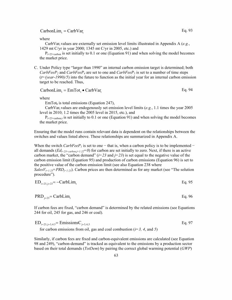
63

tt CarbVarCarbonLim = Eq. 93

where CarbVart values are externally set emission level limits illustrated in Appendix A (e.g.,

1429 mt C/yr in year 2000; 1345 mt C/yr in 2005, etc.) and Pi=23=carbon is set initially to 0.1 or one (Equation 91) and when solving the model becomes

the market price. C. Under Policy type “larger than 1990” an internal carbon emission target is determined; both

CarbFeeP2 and CarbFeeP4 are set to one and CarbFeeP5 is set to a number of time steps (t=(year-1990)/5) into the future to function as the initial year for an internal carbon emission target to be reached. Thus,

ttt CarbVarEmTotCarbonLim •= Eq. 94

where EmTott is total emissions (Equation 247), CarbVart values are endogenously set emission level limits (e.g., 1.1 times the year 2005

level in 2010; 1.2 times the 2005 level in 2015, etc.), and Pi=23=carbon,t is set initially to 0.1 or one (Equation 91) and when solving the model becomes

the market price. Ensuring that the model runs contain relevant data is dependent on the relationships between the switches and values listed above. These relationships are summarized in Appendix A. When the switch CarbFeeP1 is set to one − that is, when a carbon policy is to be implemented − all demands (Edi=23=carbon,j=1:22=0) for carbon are set initially to zero. Next, if there is an active carbon market, the “carbon demand” (i=23 and j=23) is set equal to the negative value of the carbon emission limit (Equation 95) and production of carbon emissions (Equation 96) is set to the positive value of the carbon emission limit (see also Equation 238 where SalesVi=1:23=PRDj=1:23). Carbon prices are then determined as for any market (see “The solution procedure”).

t23j,23i CarbLimED −=== Eq. 95

t23j CarbLimPRD == Eq. 96

If carbon fees are fixed, “carbon demand” is determined by the related emissions (see Equations 244 for oil, 245 for gas, and 246 or coal).

5,4,3j5.4,3j,23i EmissionsCED === = Eq. 97 for carbon emissions from oil, gas and coal combustion (i=3, 4, and 5) Similarly, if carbon fees are fixed and carbon-equivalent emissions are calculated (see Equation 98 and 249), “carbon-demand” is tracked as equivalent to the emissions by a production sector based on their total demands (TotDem) by pairing the correct global warming potential (GWP)

64

values of the different gases with the type of gases emitted (as related to their emission coefficients, EMC) and their conversion factors of monetary units to energy units (PRconvrt)

∑ •••====i

iiiij22:1j,23i EMCGWPPRconvrtTotDemEmissionsED Eq. 98

Carbon permit trade If carbon permits are traded, the value of CrbTradet can be set exogenously in the base year (variable CrbTrExot). Alternatively, under each of the carbon policy implementations listed in the previous section, CrbTradet may be based on a fixed permit price (Pi=23,t) or a market price for carbon and on a carbon emission limit set exogenously or endogenously. Carbon permit trading only takes place when regions are linked through trade markets.

( )ttregiont,23it EmTotCarbLimExchRatePCrbTrade −••= = Eq. 99

where Pi=23,t is the carbon price at time t ExchRatet is the exchange rate, CarbLimt is the emission limit, and EmTott is total carbon emissions, which are calculated in Equations 244-247.

Carbon policy impacts Impacts of carbon policies can include the following: (a) energy prices are impacted by adding the carbon fee to the energy price (see Equation 10); and (b) household, government and investment demands are impacted by accounting for a carbon fee per dollar of energy demand (see Equations 205, 206, and 140). Carbon fees collected can be recycled as revenue in various ways, described below. If carbon prices are market-based then the household, government, and investment carbon permit fees are part of a carbon market. If carbon trade is implemented and the market demand and supply are determined by emissions (see the previous section) the domestic carbon price receipts have to be taken out of the carbon trade estimate. The costs of carbon prices are recycled as revenue when carbon prices are market-based and when they are fixed. If no carbon trade is implemented, the CrbTradet variable will equal zero (Equation 100). The carbon fees imposed on investment, households, and government are based on carbon prices (see Equation 10 for determining the Cpfi values). The carbon fees to be recycled as carbon revenue within a region are the carbon fees traded and corrected for the carbon fees levied on households, government and investments. Appendix A summarizes the carbon policy option impacts through the recycling of the revenues obtained from the carbon fees and, if active, from carbon permit trade. The details of the revenue recycling are described in the investment, household and government sections in this document.

hh27j,5gv26j,5imex25j,5tt CPermFCPermFCPermFCrbTradeCrbTrade ====== −−−= Eq. 100

65

where

Carbon fees on fuel combusted and demanded by households (CPermF5,j=27) is calculated in

Equation 199: ( )∑=

==== •=24

1ihh27j,iihh27j,5 EDCpfCPermF where Cpfi is a carbon fee per dollar

of energy demand. Carbon fees on fuel combusted and demanded by government (CPermF5,j=26) is calculated in

Equation 205: ( )∑=

==== •=25

1igv26j,iigv26j,5 EDCpfCPermF

Carbon fees on fuel combusted and demanded by investment (CPermF5,j=25) is calculated in

Equation 140: ( )∑=

==== •=22

1iinv25j,iiimex25j,5 EDCpfCPermF

where

∑ ••••= =fn

fnifnregiont,23ii GWPPRconvrtEMCExchRatePCpf (see Equation 10)

ttt CrbTradeCrbFeeTotCrbFeeTot += Eq. 101

where

CrbFeeTott are the summed carbon fees: ∑=

=27

1jj,5t CPermFCrbFeeTot

66

Chapter 8. The final demand sectors The four final demand sectors that demand and produce goods and services are

• investment • households • government • net exports.

The final demand sectors are integrated with the rest of the system (see Figure 1) through their demand for final goods from the production sectors and their supply of land, labor and capital33.

Below we describe investments followed by sections on government and household supply and demand and finally by a section on imports and exports. The export/import aspects of the final demand are integrated with the product markets by including the changes in inventory as net exports to eliminate the need for modeling inventory fluctuations.

Investment The SGM requires a fixed factor, that is, the amount of capital to be known before production can take place. To close the model, an investment mechanism is required to determine how much capital is to be allocated to each of the sectors and subsectors. New capital requirements, in turn, determine the inputs necessary to produce new capital. Capital required for new production can be determined in two ways. New investment can be determined as a function of expected profit rate and investment in the previous period. Alternatively, new investments can be based on expected profit rates and the gap between expected production levels and the potential output by existing capital stocks. Whenever a distinct product is being produced, it is represented by means of a production sector. Subsectors represent different ways of making that product. Subsectors are implemented in the SGM for electricity generation. The competition among the technologies based on expected profit rates determines the relative contributions (shares) the technologies make towards electricity generation investments and this is formulated by means of the logit share equation after McFadden (1981). In that formulation the shares of the competing fuels add to one, and are 33 Demand sector indicators Final demand sectors (j) j 24 25 26 27 Investment Net Exports General Government Consumption Household Consumption inv imex Gv Hh Primary factor supply indicators i Primary factor supply sectors 24 Land ls 25 Labor lbs 26 Capital or OVA capital or capital cost 27 Indirect business taxes or IBT ibt

67

dependent on an assumed base share value for each of the competing fuels and on the elasticities of their prices. Thus, more than one fuel source and its accompanying technology (oil-fired, gas-fired, coal-fired, nuclear, and hydro in SGM 200334) can meet the electricity generation demand. Delays with regard to investments that take more than one period before coming on line are not simulated in SGM 200335.

New investments based on expected profit rates and investments in the previous period Investment as a function of expected profit rate Eπrj,jj,t and investment in the previous period KAflowt-1 is described first.

Initial annual investments KAflow for the base year (v=t=0) and old vintages (v=-1) are input parameters, as are initial expected profit rates. Thus,

∑=

=n

1jjt,jj,jt,j KAflowK for the base year Eq. 102

0t,jj,j0t,jj,j EXPPROFrE == =π for the base year Eq. 103 When based on expected profit rate and investment in the previous period, sector-level investment in the projections for all production sectors is a function of a base rate of growth, the growth in working-age population, and the expected return to capital. This investment is calculated in relation to what the marginal dollar should earn under perfect competition (margvalue=1); the production sector-specific variable Tempj determines the earnings and Kj,t denotes the potential investment into a production sector j at time t.36 The investment calculation is then

rinv

n

1jj

rhoinvt,jj,j

n

1jj

1rhoinvt,jj,j

jt,j

rE

rETempK

•=

∑

∑

=

=

+

π

π Eq. 104

where Eπrj,jj,t is a sector or subsector’s expected profit rate at time t (see Equations 55 and 57), n denotes the number of active subsectors where n ≤ jj; the summation over jj takes place only when subsector production takes place, rhoinv is the expected profit rate exponential, which equals one in the reference case, and 34 Presently (October 2004) renewables (biomass, waste, solar, geo, wind-on shore, wind-off shore) and new technologies (coal IGCC with and without carbon sequestration and disposal, gas NGCC with and without carbon sequestration and disposal, pulverized coal with carbon sequestration and disposal are implemented in various nesting structures to achieve optional knife-edge investment behavior in the model). 35 Presently (October 2004) delayed investment is a viable option in the model and implemented for new technologies to come on line. 36 calculations concern generating a new vintage v with an indicator value of v=t

68

rinv is the expected profit rate function exponential, which equals one in the reference case, and Tempj is the variable denoting investment dependency on the change in demography, the marginal value of the dollar, and some basic assumption with regard to annual investments for all production sectors:

rinvaccinv

1t

tjj valueargm

pop_age_workingpop_age_working

scalerbasekapTemp −

−

•

••= Eq. 105

where basekapj is a production sector-specific annual investment which may be based on various assumptions:

a. basekap may be based on the production-sector-specific annual investment (KAflow) from the previous time-period, thus,

1t,jj,jj KAflowbasekap −= , or b. when the annual investment is very small, basekap is 1% of the total available annual

investment into all production sectors, thus ∑ −•=jj

1t,jj,jj KAflow01.0basekap , or

c. when subsectors are involved (electricity generating subsectors), basekapj is the summed annual investments over the subsector previous time-period’s investments:

∑ −=jj

1t,jj,jj KAflowbasekap

scaler ─ an investment accelerator ─ is a scale coefficient and has a value of 1.2, working_age_populationt at a point in time is the number of people in the working age bracket, accinv is the working age population ratio exponential, which equals one in the reference case, and

margvalue is the marginal one dollar.

New investments based on anticipated output As an alternative, the model can determine demand for capital based on the expected profit rate Eπrj,jj,t and the gap between gross output PRDj and the potential output by existing capital stocks. When old and new vintages are operated, vintage-specific gross production PRDVj,jj,v is calculated for each operating vintage for each production sector j and subsector jj. Total gross production, PRDj

37 is the summed vintage-specific production.

∑ ∑−= =

=

t

3tv

n

1jjv,jj,jj PRDVPRD Eq. 106

37 In the SGM code SalesVj is set equal to PRDj at this stage, and the ED matrix at a certain stage has diagonal elements calculated as Edi,j-PRDj; in this documentation the SalesV vector is only initialized when describing the solution algorithms (see Equation 239) and the Edi,j matrix always refers to the demand matrix. Appendix A shows complete Edi,j-PRDj matrices which solve to (close to) zero for the base year (t=0) and for year 1995 (t=1).

69

PRDVj,jj,v calculations are either based on CES or on Leontief production functions, dependent on the elasticity of substitution parameter of the production sector or subsector. Anticipated increases in investments for all production sectors are in this formulation determined by an exogenous parameter in SGM 2003 (Qprojt). This parameter functions as a multiplier to the production sector’s gross production of the previous point in time. Output needed from the to-be-invested-in new vintage Qnewj is calculated as the difference between the summed active vintage-specific production sector output and the anticipated needs calculated as the summed previous vintage-specific operating production sector output multiplied by the desired increase in production. This is expressed in the following equation:

∑ ∑∑ ∑−= =

−

−= =

−

•=

t

3tv

n

1jjv,jj,j

1t

4tv

n

1jjv,jj,jtj PRDVPRDVQprojQnew Eq. 107

A testable demand for capital TestKj to produce output needed from new vintages is calculated as the product of the desired investment Qnewj and the calculated capital-to-output ratio Capq if no subsector production takes place:

jjj,jj QnewCapqTestK •= for jj=1 Eq. 108 where Capqj,jj is the capital-to-output ratio. The capital-to-output ratio is calculated based on the CES production function given that one may assume some price elasticity with regard to investment choices. Therefore, investment decisions in the SGM are based on the CES production function assumptions and not on the Leontief production function assumptions where price elasticities are zero38.

)1/(1

tv,jj,j

t,j)1/(1v,jj,j,26i

)1/(v,jj,j,0jj,j Nr

PrCapq

ρ−

=

ρ−=

ρ−ρ

π•α•α= Eq. 109

where

38 When the elasticity of substitution (σ1) is less than 0.05 this intermediate step could be calculated based on the Leontief production funcion coefficients:

v,jj,j,26iv,jj,j,0jj,jCapq =•= λλ

This is not implemented, however. This is for theoretical reasons: one may assume some price elasticity with regard to investment choices. Therefore investment decisions in the SGM are based on the CES production function assumptions and not on the Leontief production function assumptions where price elasticities are zero.

70

πNrj,jj,v=t is the profit rate calculated based on active prices and long-run elasticities, which in the CES formulation is as follows (see Equation 72)

ρ=

µ−= α•••α= /1

v,jj,j,26i/1

v,jj,jt,jv,jj,j,0tv,jj,j ZPrπNr and for the Leontief formulation as (see Equation 73):

∑−

===

•

λλ

−•λλ

=1N

it,jj,j,i

v,jj,j,26i

v,jj,j,it,j

v,jj,j,26i

v,jj,j,0tv,jj,j PiPrπNr

These calculations are more complex, however, when subsector production is simulated. Subsector investment is simulated as a shared investment. This logit sharing is only relevant to electricity production given that this sector is the only production sectors with subsectors in the reference case. Before 2040 hydropower and nuclear power-generated electricity are determined by exogenously determined investments39. Hydropower and nuclear energy produced electricity take part in the electricity generation share equation after 2035. To calculate the investment in each of the electricity technology subsectors, the expected profit rates for the fixed (hydro and nuclear) electricity subsectors are set to zero. Then, investment is allocated at the remaining subsectors through the logit function. The logit function calculates the sectoral investment shares based on the ratio of the relative expected profitability of each of the subsectors. As a consequence, subsectors with the highest expected profit rates Eπrj,jj,v=t receive the largest share of that sector’s investment. The investment subsector shares sum to one for each production sector. The logit share equation at time t is formulated as follows:

( )∑=

=

= 3n

1jj

rhoinvt,jj,j

rhoinvt,jj,j

jj,j

rE

rEShare

π

π for j=8 and jj=1:6 Eq. 110

where Eπrj,jj,t is the expected profit rate at time t (Equation 55),

rhoinv is the logit share exponential, or elasticity, a parameter that controls the rate that investment shares change in response to changes in expected profit rates, and

n denotes the investment demands for oil, gas and coal generated electricity.

Next, the inverse of capital to output ratio QCap is calculated:

39 The history of hydroelectric and nuclear generation installations over the last two decades indicates that factors other than the cost and performance of these technologies and the demand for electricity are the main drivers determining electricity capacity installed. The penetration of these technologies is therefore modeled exogenously.

71

∑=

==

=

3n

1jj jj,j

jj,j8j Capq

ShareQCap Eq. 111

And TestKj=8 is corrected for the revised capital demands:

( )6jj5jj1t,jj,j

n

1jj j

jj,j

jj

jj,j

1t,jj,j

jj

ExoElecExoElec3Kaflow2

QCapCapqExoElec3

CapqKaflow2

QnewTestK

==−

=

−

+•+•

+

•+

•

−=

∑

∑ for j=8 Eq. 112

where n is the number of active subsectors and n ≤ jj, KAflowj,jj,t-1 is the previous time period’s annual investment (see Equation 117 for the present

period’s investment), Capqj,jj is the capital to output ratio of a production sector or subsector calculated in Equation

109 (CES production function-based), QCapj is the share dependent (based on expected profit rates) inverse of the capital to output

ratio, Qnewj is the production sector related assumed improvement factor in gross production, and ExoElecjj are the exogenously set electricity-generating annual investments (hydro and nuclear

or when more subsector investments are set exogenously∑n

jjjjExoElec ).

Finally, Equation 113 can be executed, analogous to Equation 104, and annual investment Kj,t is determined by either of the two methods.

rinv

n

1jj

rhoinvt,jj,j

n

1jj

1rhoinvt,jj,j

jt,j

rE

rETestKK

•=

∑

∑

=

=

+

π

π Eq. 113

Some sectors may have investment set exogenously (but when ExoInvstj equals one or less, no exogenous investment takes place).

jt,j ExoInvstK = Eq. 114 Since investment is allocated at the subsector jj level through a logit function, the above described logit formulation has to be executed once more to correct for the share of investment into hydro-

72

electric and nuclear generated electric production and the subsector annual investments that are set exogenously. Thus, the annual subsector investments, KAflowj for the electricty sector for hydro and nuclear and the annual sector investment Kj=8,,t denoting the potential investment into the electricity sector have to be set (Equation 115), and the recalculated shares determine the remaining subsector investments, given that those shares equal one when no subsectors are active.

jjt,jj,8j ExoElecKAflow == for j=8 and jj=5 or 6 Eq. 115 The investment into electricity is updated with the exogenously set investments.

∑=

== +=n

1jjjjt,8jt,8j ExoElecKK Eq. 116

where n ≤ jj and denotes the exogenously set investments, e.g., nuclear and hydro power generating

electricity. Capital investment for all production sectors and subsectors besides the exogenously set investments is then re-calculated as:

t,jt,jj,jt,jj,j KShareKAflow •= Eq. 117 where Sharej,jj,t are the calculated shares which equal one when there are no subsector production sectors, and Kj,t is the potential investment into production sector j. Finally, the actual annual investment in the form of capital flow is retained as total capital stock over the five-year time period as KAj,jj,t for each production sector and subsector through linearly interpolated annual flows starting with the current period and going back to the previous model solution-period:

t,jj,j1t,jj,jt,jj,j KAflow3KAflow2KA •+•= − Eq. 118

Investment in energy production The investment in energy resources is more complicated. A set of triggers function as indicators for the oil, gas, and coal production sector implementation of resource-related investment functions. At the start of the model run, fossil fuel resource and reserve40 variables for a region are initialized: 40 http://www.eere.energy.gov/: “Known resources can be classified from two standpoints: 1) purely geologic or physical/chemical characteristics – such as grade, tonnage, thickness, and depth – of material in place, and 2) profitability analysis based on costs of extracting and marketing the material in a given economy at a given time. The former constitutes important objective information of the resource and a relatively unchanging foundation upon which the latter economic delineation can be based”. “ For mineral resources, the reserve chosen for this index is the reserve

73

jj,jjj,j DrsceDrsCtmp = Eq. 119

t,jj,jt,jj,j DrsveDrsVtmp = Eq. 120 Over time, oil, gas and coal investments are turned into into available reserves (Reservej in energy units) that can be consumed; these are calculated as follows based on investments in monetary values (Eqdepj):

jjj EqdepPRconvrtserveRe •= Eq. 121 where

v=t, jj equals one, given that no subector production is active for fossil fuel production,

PRconvrtj is the energy conversion factor, converting the investment costs in monetary units to physical energy units, and Eqdepj is the investment in fossil fuel production, where

t,jj,j)1/(1

v,jj,j,26iv,jj,jv,jj,j,0jj KAZxnpEqdep ••••= −=

ραα Eq. 122 where

xnpj equals the product of the nameplate lifetime of the technology (4 in the reference case for oil, gas and coal production) and the timestep (five years for SGM 2003),

α0,j,jj,v equals one, αi,=26,j,jj,v is the vintaged capital stock scale coefficient in which technical change is

incorporated (see normalizalion in Equation 27 of Equation 25 in “The vintage alphas and incorporating technical change”).

KAj,jj,v is the active vintage-specific production sector or subsector capital, and Zj,jj,v incorporates the participation of the variable factors, where

( )∑−

=

µ−µ •α••α−=1N

1ijj,j,iv,jj,j,ijj,jv,jj,j,0v,jj,j Piecst)Pe(1Z which is calculated with

expected prices in the expected profit equation and implemented with long-run elasticities (see Equation 56),

Pej,jj is the expected commodity price (see Equation 16), Piei,j,jj is the expected price paid (see Equation 15), ρ and µ are functions of the long-run elasticity σ1, αcsti,j,jj,v equals (α0,j,jj,v

ρ•αi,j,jj,v) 1/(1-ρ), (see Equations 30-31 in the section “The vintage alphas and incorporating technical change”).

base as defined by the U.S. Bureau of Mines: ‘part of the identified resource that meets specified minimum physical and chemical criteria related to current mining and production practices, including those for grade, quality thickness, and depth. The reserve base encompasses those parts of the resources that have a reasonable potential for becoming economically available within planning horizons beyond those that assume proven technology and current economics. It includes those resources that are currently economic (reserve), marginally economic (marginal reserves) and currently sub-economic”. For fossil fuels (including uranium) the reserve chosen can be based on information supplied by the World Energy Council (WEC).

74

Note that the investments into available energy reserves are calculated with the CES production function with long-run elasticities σ1. The values of αi,=26,j,jj,v used in calculating the reserves cab be found in Appendix A. Also note that jj equals one in the reference case. The quantities of uninvested depletable resources Drscej,jj change over time, because of a combination of resource growth and investment into reserves, that is, into energy for consumption. Thus,

))sgroRe1()sgroRe1((DrsceDrsCtmpDrsce Nstep)*1nt(jj,j

Nstep*ntjj,jjj,jjj,jjj,j

−+−+•+= Eq. 123 where

DrsCtmpj,jj is an exogenous value in the base year and updated after reserves are calculated (see Equation 126), Drscej,jj is the uninvested depletable resource for which the initial value is an input parameter value (Equation 119 for the initial value),

Resgroj,jj is the calculated growth in the resource base for depletables (oil, gas, coal) as a time-dependent interpolation of initial and terminal values, as long as T, which is 5 times the number of time periods (Nstep*t), is smaller than Tresgrzi.

jj,jjj,j

jj,jjj,jjj,j Tresgrz

TsgrzRe)Tresgrz

T1(sgroResgroRe •+−•= Eq. 124

where Resgroj,jj, Tresgrzj,jj, and Resgrzj,jj are input parameters.

Calculated reserves associated with desired investment are checked to see if they exceed available reserves.

jt,jj,j serveReDrsVtmp = Eq. 125

jjj,jjj,j serveReDrsCtmpDrsCtmp −= Eq. 126 where

DrsCtmpj,jj are the available energy resource at a point in time, which are updated during the iterations finding the model solution,

DrsVtmpj,jj,t is the energy resource available at a point in time initiated with the energy resource data information (Equation 120 for the base year value) and calculated through resource investment calculations in the projections and updated through Equation 70. Resources are decreased as long as the amount of production Reserve j is less than the resources available. Note that the iterative model results for one region for each of the 12 time steps (1990 through 2050 in five-year time steps) are shown in “The solution procedure” for the resource reserves invested in to be consumed, as well as for the depletable oil, gas, and coal resources.

75

The ratio of available reserves and desired reserves is calculated as

j

jj,jserveRe

DrsCtmpservesRePct = Eq. 127

Energy sources available for consumption are set equal to the calculated available reserves, which in turn are checked for depletion when vintages are operated. (See “Checks on depletable resources” after the calculations regarding operating old and new vintages.)

jt,jj,j serveReDrsVtmp = Eq. 128 If the ratio of available reserves and desired reserves is smaller than one, investment is scaled down:

jj.jjj,j EqdepservesRePctEqdep •= Eq. 129

t,jj.jt,jj,j KAflowservesRePctKAflow •= Eq. 130 and the previously calculated investment capital over the last five years into the production sectors for oil, gas and oil is updated based of resource availability as follows:

tv,jj.jtv,jj,j KAservesRePctKA == •= Eq. 131 and the investment into reserves is set to the maximum available:

jj.jj DrsCtmpserveRe = Eq. 132 Figure 10 illustrates investment in production sectors over time in the USA. The highest level of investment is in the Everything Else sector; coke production shows the lowest level of investment. Note that the vertical axis is logarithmic-transformed. The horizontal axis shows the time line; for 1990 t=0 and for 2045 t=11.

76

Investments into Production Sectors other than Energy in the Reference Case

100

1000

10000

100000

1000000

10000000

1990 1995 2000 2005 2010 2015 2020 2025 2030 2035 2040 2045 2050

Other Ag. ETE Wood Prd. Chemicals Cement Steel NFMetals OthInd PassTran FrghtTran Grains andAnimal ProForestry Food Proce

Figure 10 Investment into production sectors over time

Investments in fossil fuel production and electricity are depicted in more detail in Figures 11 and 12. The vertical axes are not log-transformed in these figures. Results are specific with regard to the input values used (carbon fees, emission limits, technical change) and assumptions made with regard to changes in population and labor productivity.

77

Investments in Fossil Fuel Related Production in the Reference Case

0

5000

10000

15000

20000

25000

30000

1990 1995 2000 2005 2010 2015 2020 2025 2030 2035 2040 2045 2050

Crude OilNatural GasCoalCoke1 Oil RefiningGasT&D

Figure 11 Investments in fossil fuel related production over time

Investments in Electricity Production in the Reference Case

0

10000

20000

30000

40000

50000

60000

70000

1990 1995 2000 2005 2010 2015 2020 2025 2030 2035 2040 2045 2050

ElecOil ElecGas ElecCoal ElecBio ElecNuc ElecHydro

Figure 12 Investment in electricity production over time

Demand for capital

78

As part of the iterative model solution, where annual capital flow is the result of the investment equations described above, demand for annual capital Kdem j,jj by each of the production sectors and subsectors is set equal to the annual capital flow KAflowj,jj,t:

t,jj,jjj,j KAflowKdem = Eq. 133 Intermediate capital goods (i=1:22) are produced as EDi,j=inv using a fixed coefficient or Leontief production function, whose coefficients are the CapMati,j matrix whose row values i are the ShareInv coefficients which are inputs (see Appendix A).

∑ ∑= =

==

•=

n

1jj

22

1jj,ijj,jinv25j,i CapMatKdemED Eq. 134

Given that Kdemj,jj is the capital demanded by a production sector j or subsector jj and CapMati,j, are the fixed coefficients of a fixed coeficient production function, the demand equation for capital (Equation 134) can be mapped onto the Leontief demand equation (see Equation 54)

where demands are described as ∑= =

•λ

λ=

n

1jjjj,j

jj,j,26i

jj,j,ij,i KAED . The quotient of the scale factors of

the inputs to production and capital λi,j,jj/λi=26,j,jj is equivalent to the elements of the CapMati,j vector for each of the inputs, and KAj,jj is equivalent to the (demanded) investment capital Kdemj,jj. Total (summed over all production sectors) capital investment (i=26) demand is the summed demand for all capital inputs multiplied by the relevant supply prices paid:

∑ ∑ ∑= = =

====

••=

22

1i

n

1jj

22

1jt,jj,j,ij,26ijj,jinv25j,26i PiCapMatKdemED Eq. 135

Total investment demand needed for GNP accounting is:

∑ ∑ ∑= = =

•=

22

1i

n

1jj

22

1jj,ijj,jt CapMatKdemKtot Eq. 136

Additional costs towards demands Transportation demands and distribution costs, WHSLi and TRNPi, are added to the final Everthing Else demands:

∑∑==

== ++=22

1ii

22

1iij,ETEij,ETEi TRNPWHSLEDED Eq. 137

where

79

WHSLi is the summed over all adjustment factors to the supply sectors calculated when operating production sector vintages (see Equation 82) and when household consumption is calculated for j=27 (Equation 193 for j=27, v=t, and n=1):

( ) ( )[ ]

( ) ( )[ ]

•+••+•−

+

•+••+•−=

====

==

=========

= −= ==

∑ ∑ ∑

t,1jj,hh27j,ETEi

hh27j,i

1jj,hh27j,i1jj,hh27j,iit,it,it,1jj,hh27j,i

22

1j

t

3tv

n

1jjt,jj,j,ETEi

v,jj,j,i

jj,j,ijj,j,iit,it,it,jj,j,i

i

PiED

TxaddTxproImExTrP1adj

PiEDV

TxaddTxproImExTrP1adjWHSL

Eq. 138 where

v refers to all actively operating vintages (v=t-3:t-1 for old vintages and v=t for new vintages), n is the number of subsectors with n ≤ jj, j is the number of production sectors, i refers to input sectors, adji,j,jj,t, is a time-period-dependent adjustment factor that reflects markups and intra-regional

transport costs, Pi,t is the market price, Tri,t is a time-period-dependent supply sector transportation cost factor, ExImi is the transportation cost rate parameter, Txproi,j,jj is a proportional tax rate on the ith product, Txaddi,j,jj is an additive tax on the ith product, EDVi,j,jj,v denotes demand by a vintaged production sector or subsector, and Pii=ETE,j,jj,t is the price paid by the producer for Everything Else input.

and

TRNPi is the summed over all supply sector transportation costs calculated when old vintages are operating (see Equation 83) and when household consumption is calculated for j=27 (Equation 194 for j=27, v=t, and n=1):

••

+

••=

===

==

= −= = =∑ ∑ ∑

t,jj,hh27j,ETEi

hh27j,iit,i

22

1j

t

3tv

n

1jj t,jj,j,ETEi

v,jj,j,iit,ii

PiEDImExTr

PiEDVImExTrTRNP

Eq. 139

Final carbon permit fees, CPermF5,j, are a function of the energy demands and the carbon fees per dollar of energy use, which are a function of the global warming potential and the emission coefficient of the fuel combusted and demanded by investments (see Equation 10 for the calculation of Cpfi). Thus,

80

( )∑=

==== •=22

1iinv25j,iiinv25j,5 EDCpfCPermF

Eq. 140

Households A great many operations are carried out in the model’s household sector. The household sector concerns

• Labor supply • Land supply • Household savings • Household demand for final products.

Demographic characteristics are the basis for household behavior as a representative consumer with regard to labor supply, land supply, savings, and demand for final products. Household income is derived after adjusting for taxes and government transfers. Income is then split between savings and expenditure, with a savings function that depends on the interest rate. Labor supply, land supply, household income and savings, and household demand for final products are described below. In the subsequent discussion, personal income in the household sector is the regional population’s total income, and households are the total regional population. The household demands include demands for land and labor, and household consumption.

Labor supply Labor supply depends on regional demographics. The SGM tracks population within each region by gender and five-year age cohort. Population data may be read in directly, using projections from either the World Bank or the United Nations for the model base year and for all future SGM time steps. This is the usual way of specifying population in the SGM (see Appendix A for data used). Alternatively, a demographics module that uses an age-cohort method of calculating population by age and gender for each region can be incorporated. The required input variables are fertility, migration, and mortality rates. The demographics module keeps track of population within each region by gender and five-year age cohorts. Base year populations may evolve by applying assumptions with regard to survival rates, fertility rates, and migration rates. For any time period, total population (of a region) is given by

( )∑=

+=NAGE

1agefemales,agemales,agetot POPPOPPOP Eq. 141

where POPage,,males is the number of males in age group age, POPage, females is the number of females in age group age, and NAGE is the number of age groups defined, which equals 16.

81

The fraction of the population that is either over 15 years old or under 65 is calculated to obtain the fraction of the population potentially in the labor force as wage earners. Thus,

( )∑=

=

+=13age

4agefemales,agemales,agetot POPPOPpop_age_working Eq. 142

or

( )∑=

=

=13age

4ageng,ageng POPpop_age_working Eq. 143

where the male and female population is summed between ages 16 and 65, that is age groups 4

through 13, and ng is either the male or female population.

Labor supply is gender-specific, which is denoted by the subscript ng. Labor supply for the projections is calculated in the SGM using the following equation:

)]Pi

PLBexp(1[LBpop_age_working1ED

t,jj,27j,ETEi

t,lbs25ing,1ng,0

ngnghh27j,lbs25i

==

====== •−•••−= ∑

Eq. 144 where

when j equals 27, representing the household sector, jj equals one by definition, ng is either male or female, LB0,ng is the maximum potential share of the gender-specific working age population

employed in any given year, working_age_popng is the gender-specific working age population (ages 15 to 64) (calculated

from the age-specific numbers of people, (see Equations 145 and 146 or read in), and

•−

==

== )Pi

PLBexp(1

t,jj,27j,ETEi

t,lbs25ing,1 denotes the labor supply responsiveness,

where Pi=25,t is the average annual wage rate (calculated initially from the input-output table by

dividing total labor supplied (hh27j,lbs25i

lbs25it,lbs25i ED

XSP====

==== = see Equation 1 and 7) and equals the

market price wage rate during the model solution process, and Pii=ETE,j=27,jj,t denotes the price of the numeraire sector.

The labor supply function parameters LB are determined as follows: the maximum potential share of the gender-specific population in the labor force for the base year LB0,ng is either fixed by an exogenous parameter or calculated from data:

tot

ngng,0 POP

pop_age_workingLB = Eq. 145

82

LB1,ng is a labor supply function coefficient in the labor supply responsiveness equation, which can be formulated as follows and although gender-specific is equal in this case for both male and female:

( )t,lbs25i

ng,0tot

hh27j,lbs25i

ng,1 PLBpop_age_working

ED1log

LB==

====

•−

= Eq. 146

where Edi=25=lbs,j=27=hh is the total demand for labor supply (see also Equation 152 below), which is set

exogenously for the base year, and calculated for projections as in Equation 147. Alternatively, to make calibration to a prescribed path simpler, the labor supply function coefficient LB1,ng can be calculated as a ratio of the labor supply and the working-age population. Under this alternative labor supply elasticity is in effect eliminated.

tot

hh27j.lbs25ing,1 pop_age_working

EDLB ===== Eq. 147

where EDi=25,j=27 is the total labor supply to be provided by households and is determined by the wage

rate (see Equation 144). Labor produced, SalesVi=25=lbs, is set equal to the negative value of labor supply demand such that the market calculations can be performed when solving the model for supply and demand

hh27j,lbs25ilbs25i ED1SalesV ====== •−= Eq. 148 The fraction of labor demand that is the demand for household’s own labor LB2,2 is calculated as follows:

t,lbs25ihh27j,lbs25i

hh27j,lbs25i2,2 PED

XLB

======

====

•= Eq. 149

where Xi=25,j=27 is labor demand by households in the base year, Edi=25,j=27 is total labor supplied by households, and Pi=25,t is the market price of the average annual wage rate during the model solution process,

and Edi=25,j=27* Pi=25,t is total payment for labor. The number of households, Nhh, in a regional population can be calculated based on the average number of people per household, pphh, as input, in the following equation:

hhpp

POPNhh tot= Eq. 150

83

where Nhh is the number of households, POPtot is the total population in a region, and pphh is the average number of persons per household.

Alternatively, if the number of households, Nhh, are known, the number of people per household, LB2,1, can be calculated:

NhhPOP

LB tot1,2 = Eq. 151

Note that next the LB1,1, LB1,2, LB2,1, and LB2,2 values are set constant over time, initially (after the base year calculations), but are then recalculated when projections are made.

Land (agricultural land) supply Households supply land on the basis of a land rental rate, where the land supply denotes the total land area that could be managed for agricultural or other purposes. SGM 2003 has one land type.41 Demand for land supply in the base year is regional input data (see Appendix A for data examples) and is calculated for projections in a parallel fashion to the demand for supply of household labor:

)]Pi

PRexp(1[RTLA1ED

t,jj,hh27j,ETEi

t,ls24i10hh27j,ls24i

===

====== •−•••−= Eq. 152

where TLA is the total land area that could be managed for agricultural or other purposes, R0 is the maximum potential share of land supplied to the market for the base year, and

•−

===

== )Pi

PRexp(1

t,jj,hh27j,ETEi

t,ls24i1 denotes the land supply responsiveness,

where Pi=24,t is the average annual rental rate of a unit of land, initially calculated from the input-

output table information (hh27j,ls24i

ls24it,ls24i ED

XSP====

==== = ; see Equations 1 and 6), and equals the

market price land rental during the model solution process, and Pii=ETE,j=27=hh,jj,t is the price of the numeraire sector.

The land supply function coefficients R are determined as follows: The maximum usable land, expressed as a fraction of land in a region R0 is input data for the base year (see Appendix A for values). R1 is a land supply function coefficient in the land supply responsiveness equation.

41 The land supply coefficients R have, therefore, no j subscripts

84

t,ls24i

0

hh27j.ls24i

1 PR

TLAED

1log

R==

====

−

= Eq. 153

where TLA is total regional available land area,

R0 is the maximum useable land for the region, which is input data for the base, and Pi=24,t is the market price of the land rent during the model solution process, EDi=24=ls,j=27=hh represents the demand for land use or land supply, which for the base year is

regional input data, and is calculated for projections as described above (Equation 152). Produced availability of land, SalesVi=24=ls, is set equal to the negative value of the demand for land supply such that the market calculations can be performed when solving the model for supply and demand.

hh27j,ls24ils24i ED1SalesV ====== •−= Eq. 154 When land rental income is calculated, the relationship, R2, between land demanded and land rental price is important; R2 is calculated as follows from the initial elements of the input-output matrix:

t,ls24i

hh27j,ls24i2 PNhh

XR

==

====

•= Eq. 155

where Xi=24,j =27 is the land demanded by households in the base year, Nhh is the number of households at time t, and Pi=24,t is the market price of land rent during the model solution process.

Note that the R0, R1, and R2 values are set constant over time, initially (after the base year calculations), but are then recalculated when projections are made.

Personal income or household income Personal income Pinc (Equation 156 and updated in Equations 171-175 and 188) equals the sum of retained income HHinc1 (Equations 157-160), labor income HHinc2 (Equation 166) and land rental income HHinc3 (Equation 168) minus personal income tax (calculated by means of the tax rate coefficient PItr) to which government transfers GovTr (Equation 170) are added and personal savings (Equation 179) are subtracted (Equation 180). Personal income calculated thus, is saved in a household consumption variable Const (Equation 181) to be part of GNP balancing at time t (Equation 236). Personal income, government transfers and savings are calculated sequentially, starting with personal income based on retained income HHinc1, labor income HHinc2, land rental income HHinc3 and taxation on personal income PItr (Equation 157). Retained income HHinc1 may be impacted by the recycling of carbon revenues, depending on if and which carbon policy is implemented (Equations 171-175). Next, government transfers are calculated based on this

85

income, but without taxation (Equation 170). Depending on if and which carbon fee policies are implemented, household income is updated based on recycling of carbon revenues. Household savings HHinc8 are calculated based on taxed income; they are in effect demand for capital by households (Equation 176) and dependent on the capital interest rate Pi=26. Savings are subtracted from income. After these updates, household consumption is set equal to household income. Household income is once more updated in Equation 188 by labor (HHinc9) and land (HHinc10) expenditures (see Equations 189 and 190). A budget constraint calculation based on that updated household income (Equation 191) limits all household demands EDi,j before a model solution can be sought. Thus, the first step in calculating household income is as follows:

t321 GovTr)PItr1()HHincHHincHHinc(Pinc +−•++= Eq. 156 where

PItr is the personal income tax rate, HHinc1 is retained household income, HHinc2 is labor income, HHinc3 is land rental income, and GovTrt are government transfers in the base year,

which are all explained below. HHinc1 is the retained household income, which in the base year (see Equation 157) is calculated from the production sector- and subsector-specific retained household earnings parameters RE0,j and the demands by the production sectors and subsectors for capital Xi=26,j,jj, restrained by taxes Citr and Xitcj and the market interest rate Pi=26. In the projections retained income is based on profits in the production sectors (see Equation 160). For the base year:

( ) ( )( )∑ ∑=

==

=

•−•−•+−•

=

22

1jt,26ij,1j,0j

6

1jjjj,j,26i1 ))PREexp(1(RE1Xitc)Citr1(XHHinc

Eq. 157 where for each production sector

∑Xi=26,j,jj is the summed subsector demand for capital by the production sector in the base year, Citr is the corporate income tax rate (see Appendix A for values), Xitcj is the production sector and/or subsector tax credit rate or dividend, which can be

initiated by setting a switch and which impact is dependent on demand. Tax credits are not activated in the reference case. The equation is shown for potential implementation, replacement or elaboration:

[ ]∑=

•=n

1jjjj,jjj,jj KdemXITCrateXitc Eq. 158

where XITCrate is the investment tax credit rate (set to zero), and

86

Kdemj,jj is the sector and subsector specific demand (see Equation 133 when final capital demand for each production sector and subsector has been determined and Equation 71 under “Checks on depletable resources,”)

Pi=26,t is the capital cost interest rate, RE0,j is the maximum retained earnings for the base year, which is a production sector-specific

input parameter, RE1,j is the production sector-specific retained household earnings parameter, which is (for the

base year 1990) calibrated against input data (through the Total corporate Retained Earning parameter, TREte).

26i

jj,0j,capital26i

j,1 P

)Citr1(REX

TREte1log

RE=

==

−••−

=∑

Eq. 159

where TREte is the total corporate retained earnings, which is read-in for calibration in the base

year and calculated for the projections (see Equations 161-164 below), Xi=26,j denotes the demand for capital by each production sector, and demands by

investment, households, government and trade in the base year. The RE0,j and RE1,j values are set constant over time after the base year calculations but are then recalculated when projections are made. For projections, retained income HHinc1 is based on profits in the production sectors:

( ) ( )( )∑ ∑=

==

−•−•+−•

π=

22

1jt,26ij,1j,0j

6

1jjjj,j1 ))P*REexp(1(RE1Xitc)Citr1(HHinc Eq. 160

where π j,jj is the production sector or subsector profit summed over the actively operating vintages:

v,jj,j

1t

3tvv,jj,jjj,j NOPctDeplete π+π•=π ∑

−

−=

where PctDeplete is calculated as not equal to one (see Equation 67) if depletable resources have

reached a depletion level when old vintages are operated, πOj,jj,v is the profit from operating old vintage production sectors or subsectors (see Equations

57 and 58), πNj,jj,v is the profit from operating new vintage production sectors or subsectors (see Equation

72), and

87

RE1,j are the production sector- and subsector-specific retained household earnings, which are recalculated through Equation 159 with a recalculated total corporate retained earnings (TREte) where

[ ]∑=

=22

1jjREteTREte Eq. 161

where

( ) ( )( ))PREexp1(REXitcCitr1REte t,26ij,1j,0j

6

1jjjj,jj =

=

•−••

•−•

π= ∑ Eq. 162

Retained income HHinc1 might be impacted by the recycling of carbon revenues, depending on if and which carbon policy is implemented (Equations 157-160). If carbon pricing is simulated, corporate earnings have to be adjusted in accordance with the carbon policy implemented. Among the options explored are the impacts of carbon policies on corporate earnings, e.g., carbon revenue recycling of 60% towards industry and 40% to households (ICRBfeeOPT=4) or all are recycled to industry (ICRBfeeOPT=6). Case 4: 60% of the domestic carbon fees are recycled towards industry and 40% to households.

tt ExIBT6.0CrbFeeTot6.0TREteTREte •+•+= Eq. 163 Case 6: all of the carbon fees are recycled to industry if the CrbFeeRcyPct3 is on.

t3t3 ExIBTctCrbFeeRcyPCrbFeeTotctCrbFeeRcyPTREteTREte •+•+= Eq. 164

where CrbFeeRcyPct3 refers to a fraction.

CrbFeeTot is based on domestic carbon fees and carbon permit trade (see Equation 101), ExIBT is the amount of IBT tax collected above the base year, which remains independent of

any carbon fee recycling. No increases in IBT taxes occur if TxIBT is constant over time.

( )∑=

=−•=22

1j0t,jt,jjt )TxIBTTxIBT(SalesPExIBT (see Equation 209) and

where TxIBTj is the production sector-specific indirect business tax, and SalesP,j is gross production summed over all active vintages and production subsectors in

monetary terms: ( )∑ ∑−= =

•=

t

3tv

n

1jjt,jv,jj,jj PrPRDVSalesP (see Equation 208).

The tax on profits produced in the production sectors Tax3,j=1:22 is kept track of in a tax array as follows:

jj22:1j,3 XitcCitrTax −π•== Eq. 165 where

88

Xitcj is production sector and/or sub sector tax credit rate or dividend (see Equation 158), and Citr is the corporate income tax rate, and

πj are the production sector profits after summing over the operating vintages and subsectors. HHinc2 is labor income, which is estimated based on demand for labor supply, social security taxes and the market price for labor:

t,lbs25ihh27j,lbs25i2 PED1)SStr1(HHinc ====== ••−•−= Eq. 166 where

SStr is the social security tax rate, which is a regional input parameter for the base year, EDi=25,j=27 is the labor supply demanded, which is described above, including its changes when

projections are calculated, and Pi=25,t is the market price of labor rental.

The social security tax is kept track of in a tax array as Tax2,j=27 and is also called HHinc5

[ ]t,lbs25ihh27j,lbs25ihh27j,2 PED1SStrTax ======== ••−•= Eq. 167 HHinc3 is land rent income, which is calculated based on demand for land supply Edi=24,j=27 (Equation 152) and the market price of land rental Pi=24=ls. Land supply may change over time through the land-use modifying parameter R2 (see Equation 155) as do the number of households Nhh (Equation 150). Note that SGM 2003 has one land type.

t,ls24ihh27j,ls24i3 PED1HHinc ====== ••−= Eq. 168 where

Edi=24,j=27 is the demand for land supply, which is described above (Equation 152), including its changes when projections are calculated, Pi=24,t is the market price for land rental during the model solution process, Nhh is the number of households, which may also change over time, and

R2 is a parameter that is based on land demanded by households and land rental price (see Equation 155), which determines land rent income. The personal income tax Tax3,j=27 is also called HHinc4.

Pitr)3HHinc2HHinc1HHinc(Tax hh27j,3 •++=== Eq. 169 where

PItr is the personal income tax rate. GovTrt are government transfers in Equation 156, which are either input parameters (see Appendix A for base year values) or calculated. GovTr are also called HHinc6. When government transfers are calculated for the base year (for t=0) and for projections, they are calculated based on per capita income Pinc (Equation 156), percent of population in young and

89

old age groups YngOld, and the fraction of the population working working_age_pop. Government transfers are assumed to be untaxed.

( )

•

•−

•

++••

•=====

=

3g2g

hh27j,lbs25i

1g

tot

3210tot

t,ETEit

YngOldpop_age_working

ED1

POPHHincHHincHHincGovTrPOP

PGovTr Eq. 170

where the exponents g1, g2, and g2 equal zero in SGM 2003, and

YngOld denotes the non-employable population, that is the population under age 15 and over age 65, and the other parameters are described above. Depending on if and which carbon fee policies are implemented, household income is updated based on recycling of carbon revenues. If carbon pricing is implemented household income has to be adjusted in accordance with the carbon policy. CrbFeeTott represents the carbon fee at time t. The different carbon policy case impacts on household income (ICRBfeeOPT=case) are shown below: Case 3: all carbon fees are returned to household income.

tCrbFeeTotPincPinc += Eq. 171

where CrbFeeTott is based on domestic carbon fees and carbon permit trade,

Case 4: 40% of the carbon fees are returned to household and 60% to industry.

tCrbFeeTot4.0PincPinc •+= Eq. 172

Case 5: domestic fees are returned to consumers, permits are returned to the deficit (a) if carbon trading is implemented and carbon trade provides for revenue households will

receive the difference between domestic carbon fees and the carbon trading fees.

tt CrbTradeCrbFeeTotPincPinc −+= Eq. 173

where CrbFeeTott is based on domestic carbon fees and carbon permit trade,

CarbTradet refers to the carbon permit trade.

(b) If carbon trading is a net loss, households receive the domestic carbon fees.

tCrbFeeTotPincPinc += Eq. 174

Case 6: all of the carbon fees, determined by CrbFeeRcyPct2, are recycled to households.

t2 CrbFeeTotctCrbFeeRcyPPincPinc •+= Eq. 175

where

90

CrbFeeRcyPct2 refers to a fraction.

Savings supply The savings supply or capital supply requires the determination of personal income Pinc, which includes the income from (a) providing labor services, (b) land rental, (c) retained corporate and personal earnings, (d) government transfers, and (e) possibly, recycled carbon revenue. Household saving supply for the base year is an input parameter, and changes over time are determined by using a simple exponential model. Thus,

))PSexp(S1(SPinc1ED 26i210hh27j,26i ==== ••−•••−= Eq. 176 where

Pinc is personal income (see Equation 156), S0 is the household savings function coefficient in the base year, and [ ]t,26i21 P)Sexp(S1 =••− denotes the saving supply responsiveness, where S1 and S2 are described below, and Pi=26,t is the capital cost interest rate and equals the market price during the model solution

process. The savings function parameters are determined as follows: S0 = the household function coefficient in the base year

1S1 = Eq. 177 and

t,26i

0

hh27j.capital26i

2 PSPinc

ED1log

S=

====

•

−= Eq. 178

where EDi=26,j=27 is the household saving supply (Equation 176), Pinc is the taxed personal income to which government transfers are added (Equation 156), S0 is the household savings function coefficient in the base year, and Pi=26,t is the capital cost interest rate which equals the market price during the model solution

process. Note that the S0, S1, and S2 values are set constant over time, initially (after the base year calculations), but are then recalculated when projections are made. Household Saving (=HHinc8) is set equal to (negative) household savings.

hh27j,capital26iED1Saving ====•−= Eq. 179 where EDi=26,j=27 is the household savings supply (see Equation 176).

91

Personal income is updated next for savings expenditures. After this update, the variable represents consumption expenditures.

SavingPincPinc −= Eq. 180 Household consumption, Const, particpating in the GNP accounting as illustrated in Equation 236 below, thus accounts for personal (household) income that can be used for commodity consumption including land and labor expenditures, given that they are not subtracted as of yet (see Equations 188-190 below).

PincCons t = Eq. 181 To obtain the total demanded savings supply, the corporate retained earnings are added.

TREteEDED hh27j,capital26ihh27j,capital26i −= ======== Eq. 182 Production of capital by households SalesVi=26 is set equal to the updated produced savings supply. hh27j,capital26i26i ED1SalesV ===== •−= Eq. 183

Total household demand for variable factor inputs Household demands will be constraint by prices paid for the household variable factor inputs (i=1:22) at time t and by household income after accounting for (subtracting) household expenditures for labor and land (Equation 188). The total costs of meeting these variable-factor household demands are therefore calculated next:

[ ]∑=

====== •=22

1it,jj,hh27j,ihh27j,ihh27j PiEDDemTot Eq. 184

These summed household demands as calculated in Equation 184 are to be used to scale the demands for inputs by households (see the budget restraints simulation expressed in Equation 191).

Household demand projections Each consumption good (each i) in household consumption (demand) is assumed to have an income and a price elasticity of demand42:

i,2i,1

t,jj,hh27j,ETEi

t,jj,hh27j,i

t,jj,hh27j,ETEii,0hh27j,22:1i Pi

PiPi

PincEEDεε

•

•=

===

==

====== Eq. 185

where

42 The constant elasticity equation is found in Edmonds and Reilly (1985:248-249).

92

Pinc refers to the updated, by savings expenditures, personal income (see Equation 180), E0,i is a scaler for household demand for supplies (i) which incorporates income and price elasticities:

i,2

i,1

t,ihh27j,i

i,0 PPinc

XE ε

ε== •

=

Eq. 186 where Xi,j=27=hh is the household demand for supplies in the base year,

Pinc is household income (Equation 180), Pii=ETE,j=27,jj,t is the price of the numeraire sector, Pii,j=27,jj,t is the price of paid for inputs with regard to the household sector, Pi,t is the market price, which equals one in the base year and equals the market price

during the model solution process, ε1,j is the income elasticity, ε2,j is the supply price elasticity.

Note that the E0,i values are set constant over time first; then household (j=27=hh) fuel use changes of oil, gas, coal and electricity (i=3, 4, 5, 8) over time are calculated by means of the updated scaler which is calculated as follows:

t,hh,i

1t,hh,0t,hh,0 Factor

EE −= (unitless) Eq. 187

where Nstep

hh,it,hh,i )HHAEEI1(Factor += (see Equation 19) where

HHAEEIi,hh is a technical change parameter for household fuel use. Labor, HHinc9, and land, HHinc10, expenditures are subtracted from personal income such that personal income Pinc denotes personal income available to purchase produced commodities. Note that consumer purchases of housing are not subtracted from income in SGM 2003.

109 HHincHHincPincPinc −−= Eq. 188 where

( )hh27j,lbs25i2,2t,jj,hh27j,lbs25i9 EDLBPi1HHinc ======== •••−= Eq. 189 are the labor expenditures, and

( )NhhRPiHHinc 2t,jj,hh27j,ls24i10 ••= ==== Eq. 190 are the land expenditures,

where Pii=25,j=27,jj,t is the price of labor rental with regard to the household sector, and

93

Pii=24,j=27,jj,t is the price of land rental with regard to the household sector. Budget constraints need to be satisfied before a model solution can be sought. Therefore, household demand is restrained by the summed shared demands of all inputs as follows:

27j

j,ihh27j,22:1i DemTot

PincEDED

====

•= Eq. 191

where total demand by the household sector from the production sectors DemTotj was calculated in Equation 184, total household income Pinc was calculated in Equation 156 and updated in Equation 182, and demand by the household sector EDi,j for industry goods was calculated in Equation 185. Finally, the demand for household labor, as determined by the household labor fraction LB2,2 is subtracted from the total labor supply Edi=25,j=27 such that the labor supply available to the rest of the economy is determined.

( )2,2hh27j,lbs25ihh27j,lbs25i LB1EDED −•= ======== Eq. 192

Additional household expenditures Adjustment factors, WHSLi, for the supply sectors (representing distribution and markup factors) are calculated. All variables in this equation are described above.

( ) ( )[ ]

•+••+•−=

===

==

======

t,jj,hh27j,ETEi

hh27j,i

hh27j,ihh27j,iit,it,it,hh27j,i

i

PiED

TxaddTxproImExTrP1adjWHSL Eq. 193

where v refers to all actively operating vintages (v=t-3:t-1 for old vintages and v=t for new vintages), n is the number of subsectors with n ≤ jj, j is the number of production sectors, i refers to input sectors, adji,j,jj,t, is a time-period-dependent adjustment factor that reflects markups and intra-regional

transport costs, Pi,t is the market price;, Tri,t is a time-period-dependent supply sector transportation cost factor, ExImi is the transportation cost rate parameter, Txproi,j,jj is a proportional tax rate on the ith product, Txaddi,j,jj is an additive tax on the ith product, EDVi,j,jj,v denotes demand by a vintaged production sector or subsector, and Pii=ETE,j,jj,t is the price paid by the producer for Everything Else input.

Transportation costs for the household market for imports and exports TRNPi are calculated as follows:

94

t,jj,hh27j,ETEi

hh27j,iit,ii Pi

EDImExTrTRNP===

==••= Eq. 194

Taxes on households Tax1,j=27 are calculated as follows:

( ) ( )1Txpro)ED(absImExTrPTax hh27j,i

24

1ihh27j,iit,it,ihh27j,1 −•••+= ==

===== ∑ Eq. 195

Household subsidies Subsii equal household taxes Tax1,j but for the sign of household demand:

hh27j,1i TaxSubsid ==−= Eq. 196 Taxes on households per unit production TaxpUj=27=hh and subsidies to supplies per unit supply are calculated when the additive taxes are greater than zero.

( )∑=

====== •=24

1ihh27j,ihh27j,ihh27j EDTxaddTaxpU Eq. 197

Subsidies per unit supply SubsidpUi equal the taxes on the household sector:

hh27j,ihh27j,iii EDTxaddSubsidpUSubsidpU ==== •−= Eq. 198 Carbon permit fees CPermF5,j are a function of the energy demands and the carbon fees per dollar of energy use, which in turn are a function of (1) the global warming potential and (2) the emission coefficient of the fuel combusted and demanded by households (see Equation 13 for the calculation of Cpfi). Thus,

( )∑=

==== •=24

1ihh27j,iihh27j,5 EDCpfCPermF Eq. 199

Government

Production of government services The government is modeled as potentially producing up to three government services in a nested production function hierarchy:

• general government services, • national defense, and • education.

The number of government services modeled in an SGM region is determined by regional data availability. Government services are assumed to be produced with fixed input-output coefficients.

95

The reference case of SGM 2003 contains only one general government service and the government preference function GF is, consequently, set to one, given that no government subsectors are simulated. In the equations below we show, however, the potential implementation of different government subsectors.

1GF t:0 = Eq. 200 Government taxes and subsidies TaxGovitc=1:5 are calculated in a manner analogous to taxes and subsidies related to the production sectors. However, they are applied in a model solution iteration as paid to the government sector itself.

( )( )∑=

==== −•••+=25

1igv26j,igv26j,iit,it,iitc 1TxproEDImExTrPTaxGov Eq. 201

where when j=gv equals 26 and jj equals one by definition,

itc is the indicator for 5 potential taxes, Txproi,j=26=gv is a proportional tax rate on the government sector which equals one for all supplies in the reference case, resulting in zero taxes in the reference case (note that when j equals 26, jj equals one by definition),

Pi,t is the market price, which equals one in the base year and equals the market price during the model solution process,

Tri,t is the time-dependent transportation cost factor (see Equation 9) ExImi is the transportation cost rate parameter (these input parameters currently equal one,

EDi,j=26=gv is the demand by the government sector for capital supply. Government supply subsidies SubsidGov equal government production taxes TaxGovitc.

itcTaxGovSubsidGov −= Eq. 202 Taxes on production per unit production TaxGovpUitc and subsidies to supplies per unit supply are calculated when the additive taxes are greater than zero,

( )∑=

==== •=25

1igv26j,igv26j,iitc EDTxaddTaxGovpU Eq. 203

where Txaddi,j=26=gv is an additive tax on government supplies.

Government subsidies per unit supply SubsidpU equal the taxes on the government sector.

itcTaxGovpUSubsidpU = Eq. 204 The carbon permit fee CPermF5,j=26 is a function of the energy demand by government and the carbon fee per dollar of energy production, which is a function of the global warming potential and the emission coefficient (based on the carbon content) of the fuel combusted (see Equation 10 for the calculation of Cpfi). Thus,

96

( )∑=

==== •=25

1igv26j,iigv26j,5 EDCpfCPermF Eq. 205

Total government taxes are the summed production sector taxes to which various other taxes are added as described in detail below:

)CPermFTaxTaxTaxTax(TotTax j,5j,4j,3j,2j,1

27

1jt ++++= ∑

= Eq. 206

where Tax1,j=1:22 for production sectors are calculated when operating old and new vintages (Equation 84 for v=t-3:t),

Tax1,j=26 equals TaxGov1 (see Equation 201) calculated during the previous model solution iteration, (Tax2,j=26 equals TaxGov2 which equals TaxGov1

Tax1,j=27 equals taxes on household related to exports and imports (Equation 195), Tax2,j=1:22 for production sectors when labor taxes (i=25) are calculated (Equation 85 for v=t-3:t),

Tax2,j=27 is the labor income tax related to the social security tax rate (Equation 167), Tax3,j=1:22 is the production sectors (j) tax on profits (Equation 165), Tax3,j=27 is the tax on personal income and personal income tax rate (Equation 169), Tax4,j=1:22 equals the taxes on the production sector-specific sales:

jjj,4 TxIBTSalesPTax •= Eq. 207 where

TxIBTj is the production sector-specific indirect business tax, and SalesP,j is gross production summed over all active vintages and production subsector in

monetary terms.

( )∑ ∑−= =

•=

t

3tv

n

1jjt,jv,jj,jj PrPRDVSalesP Eq. 208

where PRDVj,jj,v is vintage and sector (and subsector, if active) specific gross production, Prj,t is the price received for the commodity produced.

The amount of IBT tax collected above the base year (ExIBTt) is based on changes in the production sector-specific business tax. If no changes in these taxes occur the ExIBTt values are zero.

( )∑=

=−•=22

1j0t,jt,jjt )TxIBTTxIBT(SalesPExIBT Eq. 209

CPermF5,j=1:22 are carbon fees calculated for old vintages and new vintage production sectors when fossil fuels are produced (Equation 90 for v=t-3:t),

CPermF5,j=25 are carbon fees based on the per dollar energy use as a function of energy demand for investments and Cpfi,, a carbon permit fee on supplies per dollar of production based on the global warming potential and the emission coefficient of a fuel (see Equation 140).

97

CPermF5,j=26 are carbon fees based on the per dollar energy use as a function of energy demand by government and Cpfi,, a carbon permit fee on supplies per dollar of production based on the global warming potential and the emission coefficient of a fuel (see Equation 205). CPermF5,j=27 are carbon fees based on the per dollar energy use as a function of energy demand by households and Cpfi,, a carbon permit fee on supplies per dollar of production based on the global warming potential and the emission coefficient of a fuel (see Equation 199). Total government subsidies are calculated by summing the supply sector subsidies towards operating old and new vintages and the government subsidies:

( ) ( )

( ) ( )1TxproEDImExTrP

1TxproEDVImExTrP1Subsid

gv26j,i

27

26jgv26j,iit,it,i

22

1j

t

3tvjj,j,i

n

1jjv,jj,j,iit,it,ii

−•••+

+

−•••+•−=

===

==

= −= =

∑

∑ ∑ ∑Eq. 210

where

the potential subsidies to the supply sectors for operating old vintages and new vintages are summed, v=t-3:t=1 (see Equations 86 for v=t-3:t), and

the last part of the equation are the government and household subsidies (is SubsidGov which are the government production taxes (see Equation 202)). Government transfers are calculated based on per capita income, percent of population in young and old age groups, and the fraction of the population working. Government transfers are assumed to be untaxed (see Equation 170 under “Household demands”) Government deficits are input data with negative values. Deficits are calculated relative to the price of the numeraire:

t,jj,gv26j,ETEitt PiGovDeftGovDeft ===•= Eq. 211

where GovDeft are input data (see Appendix A), and

Pii=ETE,j=26=gv,jj,t is the price of the numeraire sector. Government resources GovMt can now be calculated as equal to tax collections plus a government deficit less government transfers. In the base year this amounts to the sum of all inputs (supplies)

∑ ∑= =

==== =22

0i

1

1gvjjgvjjjj,gv26j0t XGovMt Eq. 212

In the projections at each point in time t the government balance is calculated. This government balance at time t is part of the GNP accounting

98

ttttt GovDeftGovTtrSubsidyTotTaxGovMt +−−= Eq. 213 where TotTaxt denotes the summed taxes on active old and new vintage production sectors in combination with various other taxes, e.g., investment, government and household taxes (Equation 208),

Subsidyt denotes the summed supply sector subsidies (Equation 86 for old vintages and new vintages production sectors) in combination with household subsidies (Equation 196 and government subsidies (Equation 202 (see Equation 210; summing takes place over the 26 supply

sectors: ∑=

=26

1iit SubsidSubsidy

GovTrt denotes the demographics and income dependent government transfers (Equation 170), and

GovDeftt denotes the government deficits, which have negative values (Equation 211). Depending on if and which carbon fee policies are implemented, government income is updated based on recycling of carbon revenues. If carbon pricing is implemented the government deficits GovDeftt and government resources GovMtt have to be adjusted in accordance with the carbon policy. The variable CrbFeeTott represents the carbon permit fees at time t. The different carbon policy case impacts on the government deficits and resources ICRBfeeOPT=case 2 through 6 are shown below: Case 2: all carbon fees produced from government resources are returned to deficit reductions. Government deficits have negative values and carbon fees and therefore have to be subtracted.

ttt CrbFeeTotGovMtGovMt −= Eq. 214

ttt CrbFeeTotGovDeftGovDeft −= Eq. 215

where CrbFeeTott is based on domestic carbon fees and carbon permit trade,

Case 3 and 4: All carbon revenues taken from government resources are returned to other sectors.

ttt CrbFeeTotGovMtGovMt −= Eq. 216

Case 5: Domestic carbon fees are returned to consumers and permits are returned to the deficit. (a) If carbon trading is implemented and carbon trade provides for revenue, government

deficits will receive the carbon fees traded in order to reduce these deficits and carbon domestic fees will be subtracted from government resources to provide for the carbon fees to be returned to households.

ttt CrbFeeTotGovMtGovMt −= Eq. 217

ttt CrbTradeGovDeftGovDeft −= Eq. 218 where

CrbFeeTott is based on domestic carbon fees and carbon permit trade,

99

CarbTradet refers to the carbon permit trade. (b) If carbon trading is a net loss, government resources provide for the domestic carbon fees,

but deficits cannot be reduced. ttt CrbFeeTotGovMtGovMt −= Eq. 219

Case 6: Government resources will produce part of the carbon fees (see also Equation 165 where CrbFeeRcyPct2*CrbFeeTott is added to household income).

( ) t32tt CrbFeeTotctCrbFeeRcyPctCrbFeeRcyPGovMtGovMt •+−= Eq. 220

Demands for goods and services by the government Calculation of government consumption GCi,gv for the base year of each supply and government sector interaction is determined by government demand and is calculated as follows:

∑∑

=

==

==

===

=1

1gvjj t,i

igvjj,gv26j,i

gvjj,gv26j,i

0t,gv26j,i P

X

X

GC Eq. 221

Note that next the GCi,gv values are set constant over time first and then government (gv=j=26) fuel use changes for oil, gas, coal, and electricity (i=3, 4, 5, 8) over time are calculated as follows:

t,gv26j,i

1t,gv26j,it,gv26j,i Factor

GCGC

==

−==== = (unitless) Eq. 222

where Nstep

gvj,it,gvj,i )GVAEEI1(Factor == += (see Equation 21) where

GVAEEIi,j=gv is a technical change parameter for government fuel use. Expenditures by the government subsectors gvjj towards government consumption is calculated as follows when based on fixed government subsector weights:

( )∑ ∑

=========

========

==

•

+•=

1

1gvjjtv,gvjj,gv26j,ETEigvjj,gv26j,capital26i

25

1itv,gvjj,gv26j,igvjj,gv26j,capital26i

gv26j

PiGC

PiGCPGC Eq. 223

The scheme for allocation of the subsector purchases across production sectors is simulated as follows:

100

( )∑=

==•−==

==−

==

•

••= 1

1gvjj

siggvjj,gv26j

sigrhogvjj,gv26j

siggvjj,gv26j

siggvgvjj26j

tgvjj

GFPGC

GFPGCGovMtGE Eq. 224

where GovMtt is the government resource balance (Equation 220), rho equals zero resulting in a value of PGC-rho*sig of one,

sig equals one, PGCj=gv,gvjj denotes the government expenditures (Equation 223), and

GFj=26=gv,gvjj, the government preference function, equals government one, given that there are no government subsectors. Government demand for each supply sector EDi=1:25,j=gv is then calculated based on government purchases. Capital demand EDi=26,j=gv by the government is treated separately. Note that in that case the price of the numeraire sector is required. Also note that government saves automatically, so government capital does not, in this version, increase demand for savings.

∑=

======= •=1

1gvjjgvjj,gv26j,igvjj,gv26jgv26j,25:1i GCGEED Eq. 225

and add government deficit to the demand for savings

tgvjj,gv26j

1

1gvjjgvjj,,gv26j,capitaligvjj,gv26jgv26j,capital26i GovDef)PGCGCGE(ED +••= ==

========== ∑

Eq. 226 and update the demand of the Everything Else sector

∑=

=========== •+=1

1gvjjgvjj,gv26j,ETEigvjj,gv26jgv26j,ETEigv26j,ETEi )GCGE(EDED Eq. 227

Imports and exports Trade is kept track of as an demand array element denoted as EDi,j=24=exim. If trade is fixed, trade quantities can be input values (Trade0,i=23 data are in Appendix A), and trade demand can be set equal to these initial trade values. The SGM offers users the option to “read in” carbon trade (into either Trade0,i=23 or into an additional trade vector Trade1,i=23).

26:1i,0exim24j,26:1i TradeED ==== = Eq. 228

101

Over time or with open markets, trade may be assumed to be the difference between production and summed domestic demand (see Equation 231), although this assumption remains part of the market solution process. In the reference case markets are not open across the regions and trade is fixed for the base year, but trade in oil and gas is calculated as in Equation 229 as the difference between demand and supply for the projections.

j

27

1jj,22:1i22:1i,1 PRDEDTrade −−= ∑

=== Eq. 229

where Edi,j represents the demand matrix43 (see Equation 80), and

PRDj represents the production vector (vector of outputs j) (see Equation 106). To calculate the trade balance, the relevant exchange rates have to be used:

region25:1i,025:1i,0 ExchRateTradeTrade •= == Eq. 230

and/or region25:1i,125:1i,1 ExchRateTradeTrade •= == Eq. 231 The export-import balance will be determined by calculating the monetary equivalent.

[ ]∑=

= •=25

1it,i25:1i,0t PTradeImExp Eq. 232

and/or

[ ]∑=

= •=25

1it,i25:1i,1t PTradeImExp Eq. 233

If carbon pricing is simulated, the export-import balance has to be adjusted in accordance with the carbon policy implemented. This implies that the carbon trade has to be subtracted from the net exports

t,23i23i,1tt PTradeImExpImExp == •−= Eq. 234

and the carbon traded has to be converted back to tons of carbon TgC (from Equation 232):

regionl23i,123i,1 ExchRate/TradeTrade == = Eq. 235

43 In the SGM code the ED matrix at a certain stage has diagonal elements calculated as Edi,j-PRDj; in this documentation the Edi,j matrix refers to the demand matrix.

102

Chapter 9. GNP accounting To ensure that the production and demand are consistent throughout the model, the SGM relies on simple economic relations for the accounting framework. GNP can be given as the price weighted sum of net production of all products, which in turn is equal to the disposition of net output among final demand sectors (Edmonds et al. 1993:303; Kim 1995:36)

tttt

N

1i

N

1jj,ijj,i ImExGovMtConsKTotEDPRDPiGNP +++=

−•= ∑ ∑

= =

Eq. 236

where at each point in time t i is an input product identifier, j is the output product identifier, N is the number of factors of either i or j; N=27 for inputs (22 variable inputs plus a carbon

option (i=23) plus land, labor, and capital as fixed inputs (M=3) and indirect business taxes and subsidies as final input; N=22 for outputs (22 production sectors; sector 23 is the carbon market);

Pii,j is the price paid by producers for inputs, PRDj is gross domestic production,

EDi,j is the demand for product i in the production of product j, and

Ktott is total investment demand (see Equation 136) Const is household consumption, which is based on retained income, labor income and related

costs, land rental income, government transfers and with savings subtracted (see Equation 181), GovMtt is government consumption, which is based on taxes, subsidies, government transfers

and government deficits (see Equation 220), ExpImt is net export, which is based on exogenous input, energy balances and time-dependent

market prices (see Equation 234). Alternatively, consistent with the input-output accounting framework, GNP can be expressed as the sum of payments to the factors of production (Edmonds et al. 1993:303; Kim 1995:36):

∑ ∑∑ ∑=

+

+== =

•+π+=

•−•=

N

1j

MN

1Nij,ij,ijj

N

1j

N

1ij,ij,ijj EDPiTXibtEDPiPRDPrGNP Eq. 237

where i is a row factor identifier (input),

j is a column factor identifier (output), Prj is the price received for commodities produced, PRDj is gross domestic production, Pii,j is the price paid by producers for inputs, EDi,j is the demand for product i in the production of product j,

and in the last part of the identity; TXibti is the indirect business tax, πi represent the profits including net interest and capital consumption allowances, M is the number of primary factors of production (labor, land, capital).

103

Chapter 10. The solution procedure The fundamental problem that the model must address is finding a set of prices that is consistent with demands by producers and consumers for goods, services, and primary factors of production when assumptions about change are made in forecasting. Thus, for any period, equilibrium will exist when a set of prices is found for which all excess demands are zero. This set of prices is not unique. Walras’ Law guarantees that if an equilibrium set of prices exists, any positive scalar multiple of those prices is also an equilibrium set of prices. Any commodity can be chosen as a numeraire, and its price can be determined arbitrarily; in SGM the commodity of the Everything Else sector is the numeraire, and its price is set to one. The number of independent market prices is always one less than the number of markets. Similarly, since the unit of measure chosen for commodities is also arbitrary, units can be chosen such that all equilibrium prices are unity in one period. When the model solution is reached, there will be a set of prices and quantities of the n-commodity market such that all n equations in the equilibrium condition will be simultaneously satisfied. At each step in the solution process, trial prices are already known because they are set by the previous time-period prices. To calculate excess demand – the difference between demand and supply – both demand and supply are determined iteratively. Demand EDVi,j,jj,v by a vintaged production sector or subsector j or jj for input i is calculated, if the production function is assumed to be a CES function, as dependent on the variable inputs (expressed in the variable Zj,jj), prices (prices received for the commodity Prj,t and prices paid for supplies Pii,j,jj,v), capital KAj,jj,v and the various technical coefficients (αi,j,jj,v and αcsti,j,jj,v) and the production sector-specific elasticities (expressed as a function of σ, in the form of ρ or µ).

( )

•••= −

−−

= )1/(1t,jj,j,i

)1/(1v,jj,j,i/1

v,jj,j

/1

v,jj,jv,jj,j,26iv,jj,j,i PiZKAEDV ρ

ρρρρ α

α (see Equations 61 and 76)

for the CES production function implementation for old and new vintages, respectively)

where

•α••α−= ∑

−

=

µ−µ1N

1it,jj,j,iv,jj,j,it,jv,jj,j,0jj,j Picst)Pr(1Z (see Equation 49)

The annual vintage-specific gross production PRDVj,jj,v by a production sector or subsector is calculated through the CES production function as dependent on the same variables.

( ) ρρρ αα/1

v,jj,jv,jj,j,26i/1

v,jj,jv,jj,j,0v,jj,j KAZPRDV •••= =−

(see Equations 63 and 77 for the CES production function implementation for old and new vintages, respectively) Demand is calculated, if the production function represents a Leontief technology (in the SGM when the elasticity of substitution (σ2) is smaller than 0.05) as dependent on gross production and the Leontief technical coefficients,

104

v,jj,jv,jj,j,26i

v,jj,j,iv,jj,j,i KAEDV •=

=λλ

(see Equations 64 and 78 for the Leontief production

function implementation for old and new vintages, respectively) where the annual vintage-specific gross production (PRDVj,jj,v) is calculated as dependent on the Leontief technical coefficients and capital.

vjj,j,v,jj,j,26i

v,jj,j,0v,jj,j KAPRDV •=

=λλ

(see Equations 65 and 79 for the Leontief production

function implementation for old and new vintages, respectively). In the case of putty-clay behavior a sector’s vintaged and projected technical coefficients for the Leontief production function (λi,,j,jj,v for i=1:25 and j=1:22) are based on the vintage technical coefficients calculated for the CES production function.

)1/(1

t,jj,j,i

t,jv,jj,j,i

)11/(1v,jj,j,0v,jj,j,i Pi

Prρ−

ρ−ρ

•α•α=λ see Equation 44 for the variable factors

and Equation 45 for the fixed factor capital

.)11/(1

v,jj,jv,jj,j

t,jv,jj,j,26i

)11/(1v,jj,j,0v,jj,j,capital26i Ka/

Pr ρ−

=ρ−ρ

==

π•α•α=λ

Vintage and subsector-production-specific demands were summed over the operating vintages and subsectors (if operating) (i=1:25; j=1:22). Thus, EDi=1:25,j=1:22 represent the demands44 by the production sectors j for inputs, i, and those for carbon (i=23), land (i=24), labor (i=25) by each production sector.

∑ ∑−= =

==

=

t

3tv

n

1jjv,jj,j,i22:1j,25:1i EDVED (see Equation 80)

where n is the number of subsectors with n ≤ jj, and v denotes the operating old and new vintages. For the final demand sectors, demand equations are described in a series of equations in the “Final Demand” sections: “Investments”, “Households”, “Government” , and “Imports and Exports” and summarized below.

EDi=1:26,j=24=exim represents demands by trade (see Equation 228), EDi=1:22,j=25=inv represents redistribution of demands for investment (Equation 134),

44 In the SGM code the ED matrix at a certain stage has diagonal elements calculated as Edi,j-PRDj; in this documentation the Edi,j matrix refers to the demand matrix.

105

EDi=26,j=25=inv represents demands for capital by investment (Equation 135), EDi=2=ETE,j=25=inv represents demands for the Everything Else sector after adjustments for

supply sector transportation costs and additional adjustment factors (Equation 137), EDi=1:25,j=26=gv represents demands by the government sector (Equation 225), including those

for carbon, land, and labor, EDi=2=ETE,j=26=gv represents demands for the Everything Else sector by the government sector

(Equation 227) EDi=26,j=26=gv represents demands for capital by the government sector (Equation 226) EDi=1:22,j=27=hh represents demands for supplies by households; these are income- and price-

elasticity dependent (Equation 185 and constrained for overall budget: Equation 191), EDi=24=ls,j=27=hh represents demand for land supply by households (Equation 152) EDi=25=lbs,j=27=hh represents demand for labor supply by households (Equations 144 and 192) , EDi=26=capital,j=27=hh represents demand for saving supplies by households (Equations 176 and

corrected for retained income: Equation 182).

Budget constraints for households with regard to demands are expressed in Equation 191. Gross production for each sector summed over active vintages and active production subsectors was retained in a production sector vector to be part of the model solution algorithms.

∑ ∑−= =

===

==

t

3tv

n

1jjv,jj,23:1j23:1j23:1i PRDVPRDSalesV (see Equation 106) Eq. 238

where j=i=1:23 denote the product markets (see Figure 1) Note that when carbon prices are zero a

market for carbon (for j=23) is not operated. Supplies of land, labor and savings were set equal to the negative values of the demands for land, labor and savings when describing the household sector and retained in SalesV. SalesVi=24:26 denotes the supplies to the factor markets provided by labor, land and Oher Value Added (see Figure 1): SalesVi=24=ls (i=24; m=23; land supply: see Equation 154); SalesVi=25=lbs (i=25; m=24; labor supply: see Equation 148); SalesVi=26=capital (i=26; m=25; savings supply: see Equation 183) These production sector vector elements are multiplied by conversion vectors and stored as the market-supply vector:

iim PRconvrtSalesVdPrMrk •= Eq. 239 where PRconvrt converts monetary values to energy quantities such that an energy balance will be obtained in the market solution.

106

Excess demand is calculated across all markets as the difference between demand and gross production, which determines the supply to the demand sectors, and stored as a market-excess demand vector (MrkEdm)

( ) m

27

1jij,im dPrMrkPRconvrtEdMrkEd −•= ∑

= Eq. 240

where the supply sector indicators, i=1:23, and the production sector indicators, j=1:23, map on the market indicator m. Note that the market solutions are calculated in either monetary or energy units through PRconvrt; in addition, if exchange rates are involved due to trade or multiple interacting regions, demand EDi,j and gross production PRDj are converted by the appropriate exchange rates ExchRateregion. Both demands and supplies are stored after a log transformation in a vector Xvecinewt to be checked if they fall within the elasticity bounds and meet the solution criteria for convergence.

)dPrMark(Log)dPrMrkMrkEd(LogXvec mmminewt −+= Eq. 241

If not, then for the next iteration a W matrix is inverted to calculate the new prices based on the necessary delta of the price perturbation.

deltaPdelta

dPrMrkdPrMrkSupTmp

dPrMrkMrkEd)dPrMrkMrkEd(DemTmp

W

t,i

m

m

mm

mm

j,i

−

−−

++−

=

Eq. 242

where DemTmp equals MrkEdm+MrkPrdm and SupTmp equals MrkPrdm which are values from the previous solution attempt.

The new prices feed back to the demand and supply equations and the process is reiterated until a price perturbation is found for an equilibrium solution. The process is a derivative-based Newton-Raphson search procedure (see Appendix B). The procedure converges very quickly once prices approach their equilibrium values. A simple sector-by-sector line search is used first to bring prices that are far from equilibrium close to their equilibrium values (see Appendix B). Figure 13 illustrates, for one region, the extent to which the model solution searches for the solutions of fossil fuel investments. Table 4 illustrates the variable values at the end of the last iteration of the market solving algorithms when carbon policies are based on carbon emission limits at randomly chosen time period 7.

107

Figure 13 Quantities of uninvested depletable resources and invested capital in depletable resources for one region in a case other than the reference case illustrating the well-behaved nature of the SGM

Table 4 Variable values at the end of the last iteration of the market solving algorithms when carbon policies are based on carbon emission limits For t=7 when carbon policies are based on carbon equivalent emissions and carbon

Mrk (m)

(j) MrkEd = Excess Demand

MrkPrd (note energy in ExaJoules)

Pi

SalesV (note energy in monetary

108

fees of $100 ton C (see Figure 18) Region = USA

values)

Other Ag. 1 1 0.02328 138868.0 0.91327 138868.0 C.Oil Prd. 2 3 0.00000 20.8 1.00000 47777.9 N.Gas Prd. 3 4 0.00000 21.8 1.00000 50024.8 Coal Prd. 4 5 0.00000 27.8 0.89636 27122.8 Coke Prd. 5 6 0.00000 1.2 2.17083 5933.4 [empty] 6 7 0.00000 0.0 1.00000 0.0 Elec Gen. 7 8 0.00003 20.7 1.38707 425025.0 Ref Oil 8 9 0.00000 41.9 1.72712 176722.0 Gas T&D 9 10 0.00001 36.9 1.59899 176302.0 Wood Prd. 10 11 0.14703 439236.0 0.83425 439236.0 Chemicals 11 12 0.29714 616838.0 0.85995 616838.0 Cement 12 13 0.01484 143155.0 0.91768 143155.0 Steel 13 14 0.02649 153190.0 0.90411 153190.0 NFMetals 14 15 0.03776 128960.0 0.76174 128960.0 OthInd 15 16 6.44723 5948400.0 0.85386 5948400.0 PassTran 16 17 0.92306 328508.0 1.00436 328508.0 FrghtTran 17 18 0.55866 425260.0 0.95212 425260.0 Grains and Oil Seeds 18 19 0.05353 99969.7 0.84195 99969.7 Animal Products 19 20 -0.04671 196859.0 0.67687 196859.0 Forestry 20 21 -0.21275 9553.9 0.84770 9553.9 Food Processing 21 22 -2.90778 1038580.0 0.72144 1038580.0 Carbon market for fixed carbon fee of $100 per ton carbon 22 23 0.00081 2440.6 165.66 2440.6 23 24 0.00000 0.0 0.00000 0.0 Land 24 25 -0.00001 170365.0 60.62 170365.0 Labor 25 26 71.01880 2269550.0 0.08938 2269550.0 OVA (other value added) 26 2 0.00000 14169100. 1.00000 14169100.

109

Chapter 11. Calibration procedure All SGM regions are calibrated to match base year energy consumption, carbon emissions, and economic activity. 1990 is the current model base year, and one model diagnostic is the comparison between base year model output and base year data. Base year model output should exactly match base year data from energy balance tables and input-output tables (see also Appendix A). Some SGM regions are also calibrated to match external projections on energy consumption and economic output, usually from an official government source, from the present to 2020 or beyond. This is especially true of SGM-USA, where the Annual Energy Outlook, published by the US Energy Information Administration, provides projections to 2025. We use a sequential procedure for baseline calibration of gross national product (GNP), electricity generation, and fossil fuel consumption. Various technical parameters are available in SGM to influence the time path of model output, especially autonomous time trends governing the efficiency of inputs in production processes. The first step in baseline calibration is to match GDP projections by adjusting an autonomous labor efficiency improvement parameter. The second step is to match projections of electricity generation, in units of billion kilowatt-hours, by adjusting an autonomous electricity efficiency improvement parameter in all model activities that use electricity. Third, the mix of fossil fuels within electricity generation is adjusted by varying the time path of the cost to produce electricity using oil, natural gas, or coal. Fourth, fossil fuel consumption outside of electricity generation is adjusted using fossil fuel efficiency improvement parameters in all model activities that use fossil fuels. These adjustments in efficiency and cost parameters are not independent, so the baseline calibration process is repeated at least once. This calibration process is used for baseline energy consumption and carbon emissions, but another set of parameters governs the slope of the marginal abatement cost curves. For all production processes in SGM except electricity, the elasticity of input substitution determines the rate that other inputs can substitute for carbon-intensive fuels, as the price of carbon changes relative to other prices. The electricity sector in SGM is actually a collection of production processes that represent different ways of generating electricity. A parameter in the logit sharing mechanism, that determines the market share of generating technologies, governs the rate that one technology can substitute for another as relative costs change. A set of marginal abatement cost curves is constructed by running a series of constant-carbon-price experiments in SGM, with a carbon price introduced in the 2005 time step and held constant thereafter. If any of these parameters are changed, they will affect baseline calibration and the baseline calibration process must be repeated. Conversely, some of the baseline calibration parameters mentioned earlier, especially cost parameters in the electricity sector, influence the slope of the marginal abatement cost curves.

110

Chapter 12. The energy balance and emissions One of the main functions of the SGM is to balance energy demand and supply and quantify the resulting emissions by

• accounting for baseline greenhouse gas emissions over time for a country or group of countries;

• finding the least-cost path to meet any particular emissions constraint; • providing a measure of the carbon price, in dollars per metric ton; • providing a measure of the overall cost of meeting an emissions target.

Fossil fuel emissions Emission calculations, in the SGM, are based on the amount of fossil fuel combusted and fuel-specific emission coefficients. Total demand for each of the fossil fuels is calculated first. These total demands for each region need to account for trade, for both raw fuels (oil, coal, and gas) and for refined fuels (refined oil and Gas T&D). The product of fuel-specific total demand and related emission coefficients and global warming potential (GWP) results in total carbon emissions after accounting for the fixed factor energy trade when regional markets are closed ( 26:1i,0exim24j,26:1i TradeED ==== = ; see Equations 228). Thus,

24j,i

27

1jj,i22:1i EDEDTotDem =

== −= ∑ Eq. 243

where Edi,j represents the demand for supply i by production sector j which equals the summed over the subsectors and its operating vintages’ demands (see Equation 80). Emissions for oil combustion are calculated as follows:

( )refinedoil9i,09fn3i3fn

3iioil3j

TradePRconvrtTotDemPRconvrt97.0

GWPEMCEmissionsC

=====

===

•−••

••= Eq. 244

where, EMCi is the oil-specific carbon content in million tons Carbon per exajoule of the energy

source, GWPi is the global warming potential, TotDemi is the oil-specific total demand, PRconvrtfn is the energy conversion factor, which converts the relative price in monetary units

to physical energy units; the factor of 0.97 accounts for the fact that not all oil products are combusted, e.g., tar and lubricants; PRconvert for each supply sector in each region is expressed in exajoules per million 1990 regional currency, and

111

Trade0,i=9 is either a fixed trade amounts (net exports) or calculated as the difference between production and the summed domestic demand. Emissions for gas and coal combustion are calculated similarly, but for the 0.97 factor:

( )D&TGas10i,010fn4i4fn

4iigas4j

TradePRconvrtTotDemPRconvrt

GWPEMCEmissionsC

−=====

===

•−•

••= Eq. 245

where EMCi is the gas-specific carbon content in million tons C per exajoule of the energy source, GWPi is the global warming potential, TotDemi is the gas-specific total demand, PRconvrti is the energy conversion factor, which converts the relative price in monetary units

to physical energy units, and Trade0,i=10 is a fixed trade amount (net exports) or calculated as the difference between

production and the summed domestic demand.45

( )5i5fn5i5coal5j TotDemPRconvrtGWPEMCEmissionsC ===== •••= Eq. 246

where EMC5 is the coal-specific carbon content in million tons Carbon per exajoule of the energy

source, GWPi is the global warming potential, TotDemi is the coal-specific total demand, and PRconvrti is the energy conversion factor, which converts the relative price in monetary units

to physical energy units. The summed CO2 emissions are then

∑=

=5

3jit EmissionsCEmTot Eq. 247

Other greenhouse gas emissions and non-greenhouse gases All other potential emissions (CH4, N2O, HFC, PFC, and SF6) are calculated based on “emission activities”. “Emission activity” or EmActix is a term used to describe the potential of emissions to be generated during a production process either as an industrial or an energy production process, or in agriculture. Emission activities are directly related to demand. Thus,

ixixix TotDemPRconvrtEmAct •= Eq. 248

where 45 In the code the calculations are made twice: in the energy balance subroutine and in the GHG emissions subroutines; in the energy balance subroutine oil emissions are calculated by multiplying with the 0.97 factor, which accounts for the fact that some oil products are not combusted, e.g., tar, lubricants, etc.; in the GHG emission subroutine emissions are calculated without that factor.

112

ix is mapped on the supply sector index i, PRconvrti is the emission activity energy conversion factor, which converts the relative price

in monetary units to physical energy units, and TotDemix is emission activity demand (see Equation 243).

With correct mapping of EMC, GWP and PRconvrt parameters towards the emission activities, emissions of non- greenhouse gases and other than CO2 greenhouse gases can be calculated. Total demand for each region accounts for trade. Thus, carbon-equivalent emissions are calculated based on a production sector’s emission activity, which is the product of the total demands by a production sector and a conversion factor that converts monetary units to energy units (see Equation 248), multiplied by the emission activities’ emission coefficient EMC and the emissions’ global warming potential coefficient GWP:

( )iiiij TotDemPRconvrtGWPEMCEmissions •••= Eq. 249

If these emissions are greenhouse gases, they can be added to the total emissions. If they are non-greenhouse gases they are kept separate. Emissions of gases, like CO, NOX, SOX, VOC, PM10 and emissions of black carbon can potentially be simulated in a similar fashion if and when necessary data are available linking production processes and related emissions.

Mitigation and marginal abatement cost curves The SGM has options of calculating consequences of mitigation policies. For carbon dioxide and carbon-equivalent emissions we have obtained marginal abatement cost curves (MACCs)46. These marginal abatement curves are generated exogenously, based on the relationships between carbon prices and the percents reduction in emissions, which are specific to each source and type of emission. Cost curves are defined for a variable number of points relating the carbon price (level) to a corresponding percent (fraction) reduction in emissions. The model finds the percentage reduction in emissions through linear interpolations between carbon prices. Thus, when testing the impacts of carbon prices, the SGM solves for the emission levels. Alternatively, when setting carbon dioxide emission limits or carbon-equivalent emission limits as model input, the SGM market calculates the carbon fees. Obtained revenue, in both cases, can be recycled to government, households and/or industry. These options are explained in “Carbon policies” and summarized in Appendix A. Table 5 lists the relationships between emission sources, the drivers and the control options. Table 5 Emissions sources, drivers and control options Activity Emission Driver Mitigation option Oil Combustion CO2 Total Combustion Endogenous Gas Combustion CO2 Total Combustion Endogenous Coal Combustion CO2 Total Combustion Endogenous Coal Production CH4 Coal MAC

46 DeAngelo et al. (2004); Delhotal et al. (2004); Schaefer et al. (2004); Scheele and Kruger (2004)

113

Enteric CH4 Ag Production MAC NatGasSys CH4 Gas Trans & Dist MAC OilSys CH4 Oil Production MAC Manure CH4 Ag Production MAC OthAgMeth CH4 Ag Production MAC ManureN N2O Ag Production MAC SoilN N2O Ag Production MAC Landfills CH4 Everything Else MAC OthNonAgMeth CH4 Everything Else MAC Wastewater CH4 Everything Else MAC HFC23 HFC-23 Everything Else MAC ODSSub HFC’s Everything Else MAC IndProcsN N2O Everything Else MAC MobileN N2O Everything Else MAC StationaryN N2O Everything Else MAC Aluminum PFC’s Everything Else MAC Semiconductor PFC’s Everything Else MAC Mg SF6 Everything Else MAC ElecDist SF6 Electricity MAC Soil and Forest Sequestration

CO2 NA Sequestration function47

The SGM modeling team has experimented with regard to joint product production in the gas production sector (methane and natural gas). Emission mitigation technology involves multiple sectors in this case. The level of mitigation might be determined by an expected profit rate calculation done on the margins between mitigation levels provided (Mark Jacobsen 6/12/00 & 7/13/00). The energy sectors are made to bear the mitigation costs. In the joint-product mitigation case only activities in the left column (see lists below) are mitigated and the ones in the right column are not mitigated. The fact that the industrial processes and landfills are not undergoing mitigation in this case drives the price for mitigating other sectors up when emission constraints are severe (see Figure 23 in Chapter thirteen). Mitigated activities No mitigation Oilcomb Landfills Gascomb OthNonAgMeth Coalcomb Wastewater CoalPr HFC23 Enteric ODSSub NatGasSys IndProcsN OilSys MobileN Manure StationaryN

47 In SGM 2004 sequestration offsets are an option based data thanks to personal communication with Bruce A. McCarl : mccarl@tamu.edu

114

OthAgMeth Aluminum ManureN Semiconductor SoilN Mg ElecDist

Display of results For carbon dioxide and carbon-equivalent emissions, we usually display the results as marginal abatement cost curves (MACCs). To calculate marginal abatement curves as output, the simplest method is to obtain a reference case through calibration without carbon fees imposed, and then setting carbon permit fees exogenously and evaluating the results with regard to GHG emissions. The marginal abatement curves can be generated by plotting emissions over time for each of the imposed carbon fees, e.g. Figure 14. Alternative ways of displaying results are shown in Chapter thirteen.

start +5 years +10 yearslong run

0

20

40

60

80

100

120

140

160

180

0% 5% 10% 15% 20% 25% 30%

Reduction from Baseline Emissions

carb

on p

rice

(199

0 do

llars

per

tC)

Figure 14 Marginal abatement cost curves for the United States energy system generated with a series of constant-carbon-price experiments.

115

Chapter 13. Reference case results Projections/Validation/Calibration for the USA This chapter contains reference case results and briefly reviews calibration and validation. In addition, selected results of carbon policy implementations are presented. The simulation results are not analyzed in depth. The first step in baseline calibration is to match GNP projections to an exogenous source (usually the Annual Energy Outlook) by adjusting the autonomous labor efficiency improvement parameter. GNP projections obtained from the SGM simulations can also be evaluated against historical data for validation. Results for the reference case for the US are shown in Figure 15.

Historical and Projected Normalized GNP (against 1990 values)

0.5

1.0

1.5

2.0

2.5

3.0

1980 1990 2000 2010 2020 2030

SGM 2003

Historical (CEA 2002)

AEO 2003 (linked to CEA)

Figure 15 Historical and projected normalized GNP A set of curves can be constructed by running a series of constant-carbon-price experiments in the SGM, e.g., with a carbon price introduced in the 2005 time step and held constant thereafter. CO2 emissions in units of million tons of carbon in the reference case and as response to carbon fees are shown in Figure 16.

116

Response of Carbon Dioxide Emissions to Carbon Prices

1000

1500

2000

2500

3000

3500

4000

1990

1995

2000

2005

2010

2015

2020

2025

2030

2035

2040

2045

2050

Em

issi

ons

$0 per tonC$10 perton C$50 perton C$100 perton C$200 perton C

Figure 16 CO2 emissions in units of million tons of carbon in the reference case with a zero carbon fee and the responses of CO2 emissions to carbon fees of $10, $50, $100, and $200 per ton carbon

The SGM has the option tracking GHG emissions from processes in the agricultural sector, the Everything Else sector, from the electricity generation and distribution sector, and from the distributed gas production sector (see Table 65). In that case, not only carbon dioxide emissions are calculated, but also methane, nitrous oxide, HFCs, PFCs and SF6 emissions in units of carbon-equivalents. Carbon-equivalent emissions are calculated based on a production sector’s emission activity, which is the product of the total demands by a production sector and a conversion factor that converts monetary units to energy units, multiplied by the emission activities’ emission coefficient (EMC) and the emissions’ global warming potential coefficient (GWP) (see Equation 249). Figure 17 illustrates the response of the total of carbon-equivalent (CE) emissions to a carbon fee of $100 per ton carbon compared to the response to a carbon fee of $100 per ton carbon when only CO2 emissions are impacted. Figure 18 illustrates the primary fossil fuel-specific carbon dioxide emission responses to a carbon price of $100 per ton of carbon. Coal emissions respond most strongly, followed by emissions generated from oil combustion; emissions due to gas combustion are least affected.

117

Response of Carbon Dioxide and Carbon-Equivalent Emissions to Carbon Prices

1000

1500

2000

2500

3000

3500

4000

4500

500019

90

1995

2000

2005

2010

2015

2020

2025

2030

2035

2040

2045

2050

Em

issi

ons

$0 per ton CE

$100 per ton CE

$0 per ton C

$100 per ton C

Figure 17 Response of CO2 and carbon-equivalent emissions in units of million tons of carbon to carbon fees of $100 per ton carbon

118

Response of Carbon Dioxide Emissions from Oil, Coal, and Gas Combustion to Carbon Fees

0

200

400

600

800

1000

1200

1400

1600

1990

1995

2000

2005

2010

2015

2020

2025

2030

2035

2040

2045

2050

Em

issi

ons

emissions from oil if $0 perton C

emissions from oil if $100per ton C

emissions from coal if $0per ton C

emissions from coal if $100per ton C

emissions from gas if $0per ton C

emissions from gas if $100per ton C

Figure 18 Response of CO2 emissions in units of million tons of carbon from oil, gas, and coal combustion to carbon fees of zero versus $100 per ton carbon

Figure 19 illustrates the same for all carbon-equivalent emissions from the energy producing sectors.

119

Response of Carbon-Equivalent Emissions by Various Processes to Carbon-Equivalent Prices

0

200

400

600

800

1000

1200

1400

160019

9019

9520

0020

0520

1020

1520

2020

2520

3020

3520

4020

4520

50

Car

bon-

Equi

vale

nt E

mis

sion

s oil

coal

gas

gasT&D

coal production

oil refining

from oil if $100 per ton CE

from coal if $100 per ton CE

from gas if $100 per ton CE

from gasT&D if $100 per tonCE from coal production if $100per ton CE from oil refining if $100 per tonCE

Figure 19 Response of carbon-equivalent emissions in units of million tons of carbon from energy production, energy transformation, agricultural and other production processes to carbon fees of zero versus $100 per ton carbon

When agricultural practices respond to carbon prices, the largest response is due to nitrous oxide emissions from fertilizer application, followed by methane emissions from enteric fermentation, followed by manure management. In addition landfill management impacts overall carbon equivalent emissions greatly (see Figure 20). Figure 21 shows the responses of the various industrial processes to carbon prices.

120

Response to Carbon Prices of Carbon-Equivalent Emissions from Agricultural Practices

0

50

100

150

200

250

300

1990

1995

2000

2005

2010

2015

2020

2025

2030

2035

2040

2045

2050

Car

bon

equi

vale

nt e

mis

sion

sLandfills

Enteric

SoilN

Manure

ManureN

OthAgMeth

from Landfills if $100 per tonCEfrom Enteric if $100 per ton CE

from SoilN if $100 per ton CE

from Manure if $100 per ton CE

from ManureN if $100 per tonCEfrom OthAgMeth if $100 per tonCE

Figure 20 Response of carbon-equivalent emissions in units of million tons of carbon from agricultural processes to carbon fees of zero versus $100 per ton carbon

121

Response to Carbon Prices of Carbon-Equivalent Emissions from Various Industrial Processes

0

10

20

30

40

50

60

70

8019

90

1995

2000

2005

2010

2015

2020

2025

2030

2035

2040

2045

2050

Car

bon

equi

vale

nt e

mis

sion

sMobileN

IndProcsN

StationaryN

OthNonAgMeth

HFC23

Aluminum

ElecDist

Mg

Semiconductor

Wastewater

ODSSub

from MobileN if $100 per ton CE

from IndProcsN if $100 per ton CE

from StationaryN if $100 per ton CE

from OthNonAgMeth if $100 per ton CE

from HFC23 if $100 per ton CE

from Aluminum if $100 per ton CE

from ElecDist if $100 per ton CE

from Mg if $100 per ton CE

from Semiconductor if $100 per ton CE

from Wastewater if $100 per ton CE

from ODSSub if $100 per ton CE Figure 21 Carbon-equivalent emissions in units of million tons of carbon from industrial processes responding to carbon fees

The SGM has the option of setting emission limits and letting the model solve for the carbon fee that would need to be imposed to reach that goal. Figure 22 illustrates stabilization of GHG emissions. Figure 23 illustrates the carbon fees (market prices of carbon) calculated. To meet desired carbon emission targets, three options can be exercised: (1) reduce carbon dioxide emissions from primary fuel combustion, (2) reduce emissions through mitigation of all carbon-equivalent emission processes, (3) reduce emissions through mitigation of a limited number of carbon-equivalent emission processes, that is from energy production processes and agricultural processes only (see list below). Carbon prices respond accordingly. Figure 23 shows all three responses. The high carbon price is paired with carbon-equivalent emissions that exclude those of landfills and industrial processes such that the burden of emission reductions falls on the energy sector and the remaining agricultural processes. When the carbon-equivalent emission reduction burden is spread over all carbon-equivalent emissions the resulting carbon price is very similar to when only carbon dioxide emissions are targeted. Note that after the year 2045 emission restraints were allowed to be relaxed resulting in an immediate decrease of the carbon price.

122

Mitigated activities No mitigation Oilcomb Landfills Gascomb OthNonAgMeth Coalcomb Wastewater CoalPr HFC23 Enteric ODSSub NatGasSys IndProcsN OilSys MobileN Manure StationaryN OthAgMeth Aluminum ManureN Semiconductor SoilN Mg ElecDist

Attaining Emission Stabilization Levels of Carbon Dioxide and Carbon-Equivalent Emissions

1000

1200

1400

1600

1800

2000

2200

2400

2600

2800

1990

1995

2000

2005

2010

2015

2020

2025

2030

2035

2040

2045

2050

Em

issi

ons

CEstabilization

CEstabilizationMitgas

CEstabilizationCC

CO2stabilization

Figure 22 Emission stabilization levels in units of million tons of carbon set exogenously and reached as model output

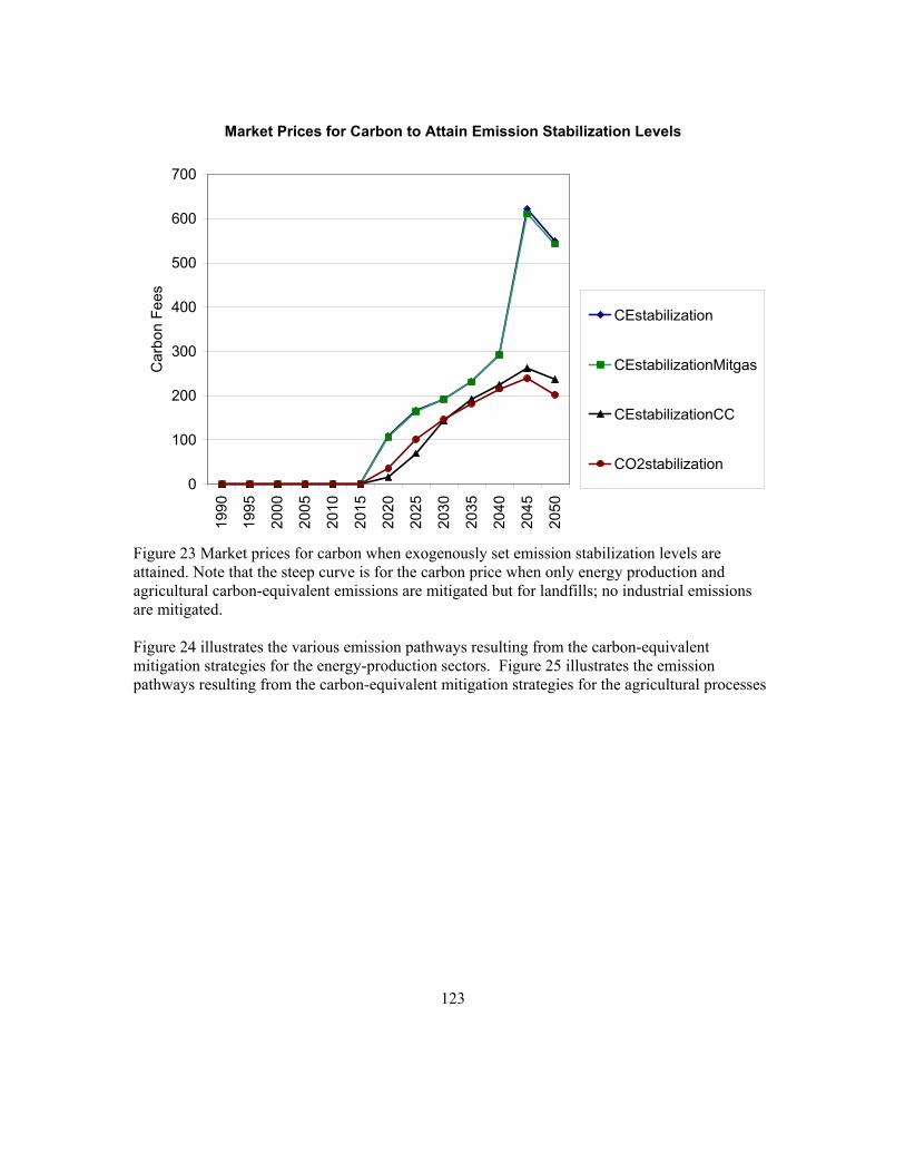
123

Market Prices for Carbon to Attain Emission Stabilization Levels

0

100

200

300

400

500

600

700

1990

1995

2000

2005

2010

2015

2020

2025

2030

2035

2040

2045

2050

Car

bon

Fees

CEstabilization

CEstabilizationMitgas

CEstabilizationCC

CO2stabilization

Figure 23 Market prices for carbon when exogenously set emission stabilization levels are attained. Note that the steep curve is for the carbon price when only energy production and agricultural carbon-equivalent emissions are mitigated but for landfills; no industrial emissions are mitigated. Figure 24 illustrates the various emission pathways resulting from the carbon-equivalent mitigation strategies for the energy-production sectors. Figure 25 illustrates the emission pathways resulting from the carbon-equivalent mitigation strategies for the agricultural processes

124

Pathways of Mitigation Through Inclusion or Exclusion of Various Sectors

0

200

400

600

800

1000

1200

1400

1600

1990

1995

2000

2005

2010

2015

2020

2025

2030

2035

2040

2045

2050

Car

bon

equi

vale

nt e

mis

sion

s Oil

Gas

Coal

oil under targets

gas under targets

coal under targets

oil under mitigation

gas under mitigation

coal under mitigation

Figure 24 Emission pathways due to the energy sectors when carbon-equivalent emission limits are imposed

125

Response of Carbon-Equivalent Emissions from Agricultural Practices to Carbon Prices

0

50

100

150

200

250

300

35019

90

1995

2000

2005

2010

2015

2020

2025

2030

2035

2040

2045

2050

Car

bon-

Equi

vale

nt E

mis

sion

sLandfillsEntericSoilNManureManureNOthAgMethLandfills under targetsEnteric under targetsSoilN under targetsManure under targetsManureN under targetsOthAgMeth under targetsLandfills under mitigationEnteric under mitigationSoilN under mitigationManure under mitigationManureN under mitigationOthAgMeth under mitigation

Figure 25 Emission pathways due to the agricultural sector when carbon-equivalent emission limits are imposed

Thus, when mitigation is implemented in the energy sectors and some of the agricultural sectors and not in landfill management nor in the other sectors, we find the energy sectors and the mitigation-active agricultural sectors much more impacted compared to when all mitigation options are activated. A considerably higher carbon price results.

Technical scale coefficients (αi,j,v) that relate “inputs to production” and the “production process” are partially determined by the elasticities of substitution in the production equations and partially dependent on the market prices resulting from solving for excess demand close to zero in the model solution process (see section on “Technical change”). Figures 26 and 27 illustrate both aspects for αi=1,j=1 − that is, for the technical scale coefficient that relate agricultural input to agricultural production. In the reference case, the technical scale coefficients are vintage dependent. When carbon prices change over time due to imposed carbon emission limits, the technical scale coefficients are affected due to changes in prices paid. Note that when emission limits are relaxed from year 2045 to 2050, responses can be seen in the technical scale coefficients as illustrated in Figure 27.

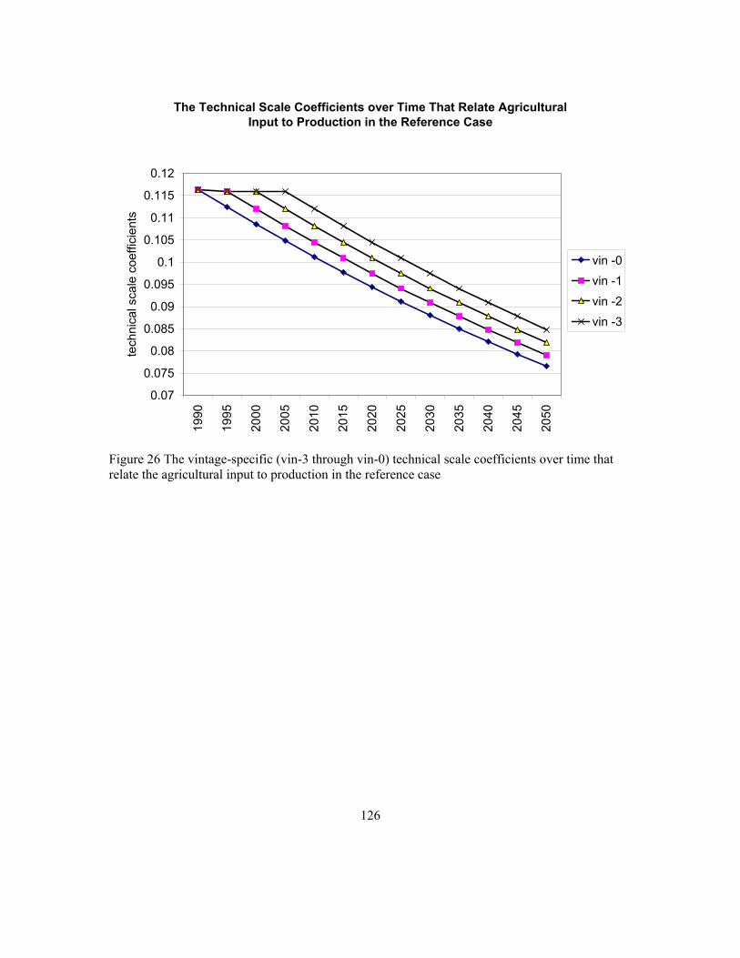
126

The Technical Scale Coefficients over Time That Relate Agricultural Input to Production in the Reference Case

0.07

0.075

0.08

0.085

0.09

0.095

0.1

0.105

0.11

0.115

0.12

1990

1995

2000

2005

2010

2015

2020

2025

2030

2035

2040

2045

2050

tech

nica

l sca

le c

oeffi

cien

ts

vin -0

vin -1

vin -2

vin -3

Figure 26 The vintage-specific (vin-3 through vin-0) technical scale coefficients over time that relate the agricultural input to production in the reference case

127

The Technical Scale Coefficients When Mitigation Is Applied for All Emitting Sectors or for Industry Only

0.06

0.07

0.08

0.09

0.1

0.11

0.12

1990

1995

2000

2005

2010

2015

2020

2025

2030

2035

2040

2045

2050

Tech

nica

l Sca

le C

oeffi

cien

ts

vin -0 CE_all

vin -1 CE_all

vin -2 CE_all

vin -3 CE_all

vin -0 CE_ind

vin -1 CE_ind

vin -2 CE_ind

vin -3 CE_ind

Figure 27 The vintage-specific technical scale coefficients (vin-3 through vin-0) over time that relate the agricultural input to production. The vintage-specific technical scale coefficients are shown (1) when all sectors are impacted by a carbon price and all carbon-equivalent emissions are mitigated (CE_all) and (2) when all sectors are impacted by a carbon price and the energy production sectors and a limited number of agricultural processes are mitigated (CE_ind) (no landfill mitigation and no industrial processes mitigation).

The second step in the calibration process is to match projections of electricity generation, in units of billion kilowatt hours, by adjusting an autonomous electricity efficiency improvement parameter in all model activities that use electricity. The results, shown in Figure 28 illustrate a combination of validation against historical data and the results of calibration of projections in model-to-model output comparisons.

128

Historical and Projected Electricity Generation in the U.S.A. (bilion KWh)

2500

3000

3500

4000

4500

5000

5500

6000

1980 1990 2000 2010 2020 2030

biill

ion

KW

h

Annual Energy Review(total)

AEO (total)

Annual Energy Review(electric power)

AEO (electric power)

SGM 2003

Figure 28 Historical and projected electricity generation in the USA. in billion kilowatt hours

The total amount of CO2 emissions generated by the electricity production sector is directly related to the total amount of electricity generated, but more specifically by what fuels are combusted. The mix of fossil fuels within electricity generation is adjusted by varying the time path of the cost to produce electricity using oil, natural gas, or coal in the calibration process. Consequences of these adjustments manifest themselves not only in the total amount of CO2 emitted but also in the fuel-specific emission balance (see Figure 29). Moreover, when carbon fees are imposed, this emission balance is affected also. Figures 30 and 31 illustrate the CO2 emissions over time from the combustion of fossil fuels for electricity generation for the reference case and for when $100 per ton carbon fees are imposed.

129

Historical and Projected Carbon Dioxide Emissions from the Combustion of Fossil Fuels for Electricity Generation

450

500

550

600

650

700

750

800

850

900

1985

1990

1995

2000

2005

2010

2015

2020

2025

2030

Em

issi

ons

SGM 2003

AEO 2003

Historical reconstructionwith EIA data

Emissions of GHG in theUS 2000

Figure 29 Historical and projected CO2 emissions in units of million tons of carbon from the combustion of fossil fuels from electricity generation

130

Carbon Dioxide Emissions From the Combustion of Fossil Fuels for Electricity Generation When No Carbon Fees Are Imposed

0

200

400

600

800

1000

1200

1400

1600

1800

1990 1995 2000 2005 2010 2015 2020 2025 2030 2035 2040 2045 2050

Emis

sion

s

coalgasoil

Figure 30 CO2 emissions in units of million tons of carbon from the combustion of fossil fuels from electricity generation

131

Carbon Dioxide Emissions From the Combustion of Fossil Fuels for Electricity Generation When Carbon Fees Are Imposed of $100 per

Ton Carbon

0

200

400

600

800

1000

1200

1400

1600

1990 1995 2000 2005 2010 2015 2020 2025 2030 2035 2040 2045 2050

coalgasoil

Figure 31 CO2 emissions in units of million tons of carbon from the combustion of fossil fuels from electricity generation when carbon fees are imposed of $100 per ton carbon

132

References Chung, J.W. 1994. Utility and Production Functions. Blackwell Publishers. Chiang, A.C. 1967 Fundamental Methods of Mathematical Economics McGraw-Hill Book Company. DeAngelo, B. J., DelaChesnaye, F. C., Beach, R. H., Sommer, A. and Murray, B. C. (2004). Methane and nitrous oxide mitigation in agriculture. Energy Journal (forthcoming). Delhotal, K. C., DelaChesnaye, F. C., Gardiner, A., Bates, J. and Sankovski, A. (2004). Mitigation of methane and nitrous oxide emissions from waste, energy and industry. Energy Journal (forthcoming). Dervis, K, J. De Melo and S. Robinson. 1985. General equilibrium models for development policy. Cambridge University Press. Cambridge, London, New York, New Rochelle, Melbourne, Sydney. Edmonds, J. and Moreira (2003), Cross Cutting Theme: Technology in AR4, http://www.ipcc.ch/activity/cct7.pdf, accessed 10/13/04. Edmonds, J.A. and J. Reilly. 1985. Global Energy: Assessing the Future. Oxford, New York. Edmonds, J.A., H.M. Pitcher, D. Barns, R. Baron and M.A. Wise. 1993. ‘Modeling Future Greenhouse Gas Emissions: The Second Generation Model Description,’ in Modelling Global Change, Lawrence R. Klein and Fu-chen Lo, eds. United Nations University Press, New York. Edmonds, J.A., J.M. Roop and M.J. Scott 2000. Technology and the Economics of Climate Change Policy. Pew Center on Global Climate Change, Washington, DC. Edmonds, J.A., SH Kim, CN MacCracken, RD Sands, MA Wise. Return to 1990: The Cost of Mitigating United States Carbon Emissions in the Post-2000 Period October 1997. PNNL11819 Fisher-Vanden, K.A., R. Baron, J.A. Edmonds, H.M. Pitcher, R.D. Sands and M.A. Wise. 1993. Calibration of the Second Generation Model, draft report. Pacific Northwest National Laboratory, Washington, D.C. Henderson, James M. and Richard E. Quandt. 1971. Microeconomic Theory: A Mathematical Approach. McGraw-Hill Book Company, New York. International Energy Agency (IEA). 1996. World Energy Outlook: 1996 Edition. Organization for Economic Cooperation and Development, Paris, France.

133

International Energy Agency (IEA). 1997. Energy Balances for OECD and Non-OECD Countries, data provided on floppy disk. Organization for Economic Cooperation and Development, Paris France. Kim, Son Hwi 1995. Stabilization of carbon emissions: a viable option for the Republic of South Korea. Massachusetts Institute of Technology, Cambridge, MA. Miller, Ronald E., and Peter D. Blair. 1985. Input-Output Analysis: Foundations and Extensions. Prentice-Hall, Inc., Englewood Cliffs, New Jersey. Reister, David B., James A. Edmonds, Richard W. Barnes, The Oak Ridge Industrial Model Volume II - Model Description ORNL/Con-56/V2 Sands, R.D. 2002. SGM 2000: Model Description and Theory. Draft report. Joint Global Change Research Institute, College Park, MD. Schaefer, D. O., Godwin, D. and Harnisch, J. (2004). Estimating future emissions and potential reductions of HFCs, PFCs and SF6. Energy Journal (forthcoming). Scheele, E. A. and Kruger, D. (2004). Global antropogenic methane and nitrous oxide emissions. Energy Journal (forthcoming). ‘’United States Department of Energy, Energy Information Administration (EIA). December 1996. Annual Energy Outlook 1997: with Projections to 2015. DOE/EIA-0383(97), Washington, D.C. United States Government. May 1997. Economic Effects of Global Climate Change Policies: Results of the Research Efforts of the Interagency Analytical Team, draft report.

134

List of Equations

∑ ∑= =

=

22

1j

n

1jjv,jj,j,iv,i XXS Eq. 1

v,jj,j,27i

26

1i

n

1jjv,jj,j,iv,j XXXS =

= =

+

= ∑ ∑ Eq. 2

ρρρ ααα

/11N

1iv,jj,j,26iv,jj,j,26iv,jj,j,iv,jj,j,iv,jj,j,0v,jj,j XXq

+= ∑

−

=== Eq. 3

10 newv,joldv,j <σ≤σ≤ == Eq. 4

=

v,jj,j,N

v,jj,j,N

v,jj,j,i

v,jj,j,i

v,jj,j,1

v,jj,j,1v,jj,j,0v,jj,j

X.....

X,,

Xminq

λλλλ K Eq. 5

hh27j,ls24i

ls24it,ls24i ED

XSP====

==== = Eq. 6

hh27j,lbs25i

lbs25it,lbs25i ED

XSP====

==== = Eq. 7

∑

∑+

=

+

=+=

=

−= 1N

1iv,jj,j,i

1N

1iv,jj,j,1Niv,jj,j,i

0t,j

X

XXPr Eq. 8

( )ijj,j,ijj,j,iit,it,jj,j,it,jj,j,i CpfTxaddTxproImExPadjPi ++•••= Eq. 9

∑ ••••= =fn

fnifnregiont,23ii GWPPRconvrtEMCExchRatePCpf Eq. 10

jj,j,ijj,j,i

jj,j,ijj,j,it,jj,j,i Tadjz

TAdjz)Tadjz

T1(Adadj •+−•= Eq. 11

26it,jj,j,capitalit,jj,j,capitali PwedgePi === += Eq. 12

j

jt,jt,it,j TxIBT1

ImExTrPPr

+

•+= Eq. 13

jj

jjt,j Ttrz

TTrz)Ttrz

T1(TriTr •+−•= Eq. 14

135

( ) ( )

+−•

+•

+•=

===

expT

t,jj,j,26it,jj,j,26i

5.0

t,jj,j,26it,jj,j,ijj,j,i Pi1

11Pi

11)Pi1

1PiPie Eq. 15

( ) ( )

+−•

+•

+•=

===

expT

t,jj,j,26it,jj,j,26i

5.0

t,jj,j,26it,jjj,j,i Pi1

11Pi

11)Pi1

1PrPe Eq. 16

j,0

j,ij,ia

λλ

= Eq. 17

[ ])1/(1

i

j)1/(j,ij,0j,i p

p)p(a

−−

••=

ρρραα Eq. 18

Nstep1t,jj,j,it,jj,j,i )TECHNN1(FactorFactor +•= − (unitless) Eq. 19

Nstephh,it,hh,i )HHAEEI1(Factor += (unitless) Eq. 20

Nstepgv,it,gv,i )GVAEEI1(Factor += (unitless) Eq. 21

t,ETEi

t,i

t,ETEiv,jj,j,ETEi

t,iv,jj,j,iv,jj,j,i P

PP/XP/X

=

µρ

==

•

=α Eq. 22

µ

=

=µ−+

=

ρ−

=

•

•

=α ∑

/1

t,ETEi

v,jj,j,ETEi/11N

1iv,jj,j,i

/1

t,ETEi

jj,j,0v,jj,j,0 P

XX

PP

Eq. 23

∑

∑+

=

+

=+=−

= 1N

1iv,jj,j,i

1N

1iv,jj,j,1Niv,jj,j,i

jj,j,0

X

XXP Eq. 24

v,jj,j0

3vv,jj,j

v,jj,j,0

1N

1iv,jj,j,i

v,jj,j,26i ZKAprior

1X

•

•α

=α

ρ

−=

+

==

∑

∑ Eq. 25

∑−

= =

µ

αα

••α−=1N

1i v,jj,j,ETEi

v,jj,j,it,ijj,j,0v,jj,j,0v,jj,j P)P(1Z Eq. 26

∑=

=

α

α=α 26N

0iv,jj,j,i

v,jj,j,iv,jj,j,i for i=1:26 and j=1:22 Eq. 27

136

ρ

=

=

α

α=α

∑

/1

26N

0iv,jj,j,i

v,jj,j,0v,jj,j,0 Eq. 28

ραα t,jj,j,i1v,jj,j,iv,jj,j,i Factor•= − Eq. 29

v,jj,j,iv,jj,j,0v,jj,j,i ααα ρ •= Eq. 30

( ) )1/(1v,jj,j,iv,jj,j,icst ρ−α=α Eq. 31

1v,jj,j,0 =α Eq. 32

1cst v,jj,j,0v,jj,j,0 == •ρσαα Eq. 33 )11/()21(

v,jj,jv,jj,j

t,j)11/()21(v,jj,j,26iv,jj,j,26i KA

Prρ−ρ−ρ

ρ−ρ−==

π•α=α Eq. 34

v,jj,jv,jj,j KApriorKA = Eq. 35 )11/()21(

t,jj,j,i

t,j)11/()21(v,jj,j,iv,jj,j,i Pi

Prρ−ρ−ρ

ρ−ρ−

•α=α Eq. 36

( ) )21/(1v,jj,j,iv,jj,j,icst ρ−α=α Eq. 37

1cst 22v,j,0v,j,0 == •ρσαα Eq. 38

∑=

=

==λ N

1i0t,jv,jj,j,i

0t,jj,j,iv,jj,j,iv,jj,j,i

Pr/X

Pi/X Eq. 39

1v,jj,j,0 =λ Eq. 40

∑

∑

=

−=== =λ N

1it,jv,jj,j,i

0

3vv,jj,j

v,jj,j,capital26i

Pr/X

KAprior Eq. 41

1v,jj,j,0 =λ Eq. 42

Nstepi

1t,jj,j,it,jj,j,i )1( γ+

λ=λ − Eq. 43

)1/(1

t,jj,j,i

t,jv,jj,j,i

)11/(1v,jj,j,0v,jj,j,i Pi

Prρ−

ρ−ρ

•α•α=λ Eq. 44

137

)11/(1

v,jj,jv,jj,j

t,jv,jj,j,26i

)11/(1v,jj,j,0v,jj,j,capital26i Ka/

Pr ρ−

=ρ−ρ

==

π•α•α=λ Eq. 45

∑−

=

•−•=1N

1iv,jj,j,it,jj,j,iv,jj,jt,jv,jj,j XPiqPrπ Eq. 46

v,jj,j,i

v,jj,jt,jt,jj,j,i X

qPrPi

∂∂

•= , i=1, …N-1 Eq. 47

ρµ− •••α= /1v,jj,j

/1v,jj,jt,jv,jj,j,0v,jj,j YZPrπ Eq. 48

•α••α−= ∑

−

=

µ−µMN

1it,jj,j,iv,jj,j,it,jv,jj,j,0v,jj,j Picst)Pr(1Z Eq. 49

( )∑+−=

ρ= •=

N

1MNij,jj,jv,jj,j,26iv,jj,j KAacstY Eq. 50

v,jj,j

1N

it,jj,j,i

v,jj,j,capitali

v,jj,j,it,j

v,jj,j,capitali

v,jj,j,0v,jj,j KAPiPrπ •

•

λ

λ−•

λ

λ= ∑

−

==

Eq. 51

v,jj,j,it,jj,j,i

v,jj,j XPi

−=∂

∂π Eq. 52

ρρµ

•

α••α=

/1

v,jj,j

v,jj,j

/

t,jj,j,i

v,jj,j,it,jv,jj,j,0v,jj,j,i Z

YPi

PrX Eq. 53

v,jj,jv,jj,j,26i

v,jj,j,iv,jj,j

v,jj,j,26i

v,jj,j,0

v,jj,j,0

v,jj,j,iv,jj,j,i KAKAX •=••=

== λλ

λλ

λλ

Eq. 54

ρ=

ρ−ρ

=

α•••α=π /1v,jj,j,26i

/)1(v,jj,j

t,jj,j,ETEi

jj,jv,jj,j,0t,jj,j Z

PiePe

rE Eq. 55

( )∑−

=

−ρρρ−ρ= •α••α−=

1N

1i

)1/(jj,j,iv,jj,j,i

)1/(jj,jv,jj,j,0tv,jj,j Piecst)Pe(1Z Eq. 56

∑−

====

•

λ

λ−•

λ

λ=π

1N

ijj,j

v,jj,j,capital26i

v,jj,j,ijj,j

v,jj,j,capital26i

v.jj.j,0t.jj.j PiePerE Eq. 57

( )( ) ( ) ρρρρ αα/1

v,jj,jv,jj,j,26i

)1(/1v,jj,jjv,jj,j,01t:3tv,jj,j KAZPrπO ••••= =

−−−−= Eq. 58

v,jj,j

1N

it,jj,j,i

v,jj,j,26i

v,jj,j,it,j

v,jj,j,26i

v,jj,j,01t:3tv,jj,j KAPiPrπO •

•

λλ

−•λλ

= ∑−

==−−= Eq. 59

138

v,jj,j

v,jj,jv,jj,j KA

OπOr

π= Eq. 60

( ) ρρ=

ρ−

ρ−

−−= •α••

α••α•=

/1

v,jj,jv,jj,j,26i/1

v,jj,j

)1/(1

t,jj,j,i

v,jj,j,it,jv,jj,j,01t:3tv,jj,j,i KAZ

PiPrfacEDV ..

Eq. 61 3

v,jj,j2

v,jj,j

01.0Or

201.0

Or3fac

•−

•=

ππ Eq. 62

( ) ρρ=

ρ−−−= •α••α•=

/1

v,jj,jv,jj,j,26i/1

v,jj,jv,jj,j,01t:3tv,jj,j KAZfacPRDV Eq. 63

v,jj,j,0

v,jj,j,iv,jj,j1t:3tv,jj,j,i PRDVEDV

λλ

•=−−= Eq. 64

vjj,j,v,jj,j,26i

v,jj,j,01t:3tv,jj,j KAfacPRDV ••=

=−−= λ

λ Eq. 65

jv,jj,jv,jj,jj PRconvrt))PRDV3()PRDV2((Deplete ••+•= Eq. 66

j

t,jj,jDeplete

DRSVtmpPctDeplete = Eq. 67

v,jj,j1t:3tv,jj,j PRDVPctDepletePRDV •=−−= Eq. 68

v,jj,j1t:3tv,jj,j PctDepleteO π•=π −−= Eq. 69

jt,jj,jt,jj,j DepleteDrsVtmpDrsVtmp −= Eq. 70

jj,jjj,j KdemPctDepleteKdem •= Eq. 71 ρ

=µ−

= α•••α= /1v,jj,j,26i

/1v,jj,jt,jv,jj,j,0tv,jj,j ZPrπNr Eq. 72

∑−

===

•

λλ

−•λλ

=1N

it,jj,j,i

v,jj,j,26i

v,jj,j,it,j

v,jj,j,26i

v,jj,j,0tv,jj,j PiPrπNr Eq. 73

( )( ) ( ) ρρ=

ρ−ρ−= •α•••α=

/1

v,jj,jv,jj,j,26i

)1(/1v,jj,jt,jv,jj,j,0tv,jj,j KAZPrπN Eq. 74

v,jj,j

1N

it,jj,j,i

v,jj,j,26i

v,jj,j,it,j

v,jj,j,26i

v,jj,j,0tv,jj,j KAPiPrπN •

•

λλ

−•λλ

= ∑−

=== Eq. 75

( ) ρρ=

ρ−

ρ−

= •α••

α•α•=

/1

v,jj,jv,jj,j,26i/1

v,jj,j

)1/(1

t,jj,j,i

v,jj,j,iv,jj,j,0t,jtv,jj,j,i KAZ

PiPrEDV Eq. 76

( ) ρρρ αα/1

v,jj,jv,jj,j,26i/1

v,jj,jv,jj,j,0tv,jj,j KAZPRDV •••= =−

= Eq. 77

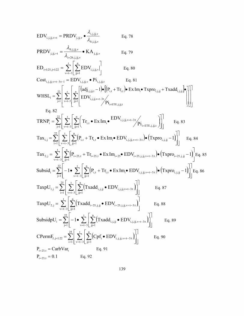
139

v,jj,j,0

v,jj,j,iv,jj,jtv,jj,j,i PRDVEDV

λλ

•== Eq. 78

vjj,j,v,jj,j,26i

v,jj,j,0t,jj,j KAPRDV •=

== λ

λ Eq. 79

∑ ∑−= =

==

=

t

3tv

n

1jjv,jj,j,i22:1j,25:1i EDVED Eq. 80

t,jj,j,iv,jj,j,i1t:3tv,jj,j,i PiEDVCost •=−−= Eq. 81

( ) ( )[ ]∑ ∑ ∑

= −= ==

−=

•+••+•−=

22

1j

t

3tv

n

1jjt,jj,j,ETEi

t:3tv,jj,j,i

jj,j,ijj,j,iit,it,it,jj,j,i

i

PiEDV

TxaddTxproImExTrP1adjWHSL

Eq. 82

∑ ∑ ∑= −= = =

−=

••=

22

1j

t

3tv

n

1jj t,jj,j,ETEi

t:3tv,jj,j,iit,ii Pi

EDVImExTrTRNP Eq. 83

( ) ( )∑ ∑ ∑= −= =

−=

−•••+=

22

1i

t

3tvjj,j,i

n

1jjt:3tv,jj,j,iit,it,ij,1 1TxproEDVImExTrPTax Eq. 84

( ) ( )∑ ∑−=

==

−=====

−•••+=

t

3tvjj,j,25i

n

1jjt:3tv,jj,j,25i25it,25it,25ij,2 1TxproEDVImExTrPTax Eq. 85

( ) ( )∑ ∑ ∑= −= =

−=

−•••+•−=

22

1j

t

3tvjj,j,i

n

1jjt:3tv,jj,j,iit,it,ii 1TxproEDVImExTrP1Subsid Eq. 86

( )∑ ∑ ∑= −= =

−=

•=

25

1i

t

3tv

n

1jjt:3tv,jj,j,ijj,j,ij,1 EDVTxaddTaxpU Eq. 87

( )∑ ∑−= =

−===

•=

t

3tv

n

1jjt:3tv,jj,j,25ijj,j,25ij,2 EDVTxaddTaxpU Eq. 88

( )∑ ∑ ∑= −= =

−=

••−=

22

1j

t

3tv

n

1jjt:3tv,jj,j,ijj,j,ii EDVTxadd1SubsidpU Eq. 89

( )∑ ∑ ∑= −= =

−==

•=

25

1i

t

3tv

n

1jjt:3tv,jj,j,ii22:1j,5 EDVCpfCPermF Eq. 90

tt,23i CarbVarP == Eq. 91 1.0P t,23i == Eq. 92

140

tt CarbVarCarbonLim = Eq. 93

ttt CarbVarEmTotCarbonLim •= Eq. 94

t23j,23i CarbLimED −=== Eq. 95

t23j CarbLimPRD == Eq. 96

5,4,3j5.4,3j,23i EmissionsCED === = Eq. 97

∑ •••====i

iiiij22:1j,23i EMCGWPPRconvrtTotDemEmissionsED Eq. 98

( )ttregiont,23it EmTotCarbLimExchRatePCrbTrade −••= = Eq. 99

hh27j,5gv26j,5imex25j,5tt CPermFCPermFCPermFCrbTradeCrbTrade ====== −−−= Eq. 100

ttt CrbTradeCrbFeeTotCrbFeeTot += Eq. 101

∑=

=n

1jjt,jj,jt,j KAflowK for the base year Eq. 102

0t,jj,j0t,jj,j EXPPROFrE == =π for the base year Eq. 103 rinv

n

1jj

rhoinvt,jj,j

n

1jj

1rhoinvt,jj,j

jt,j

rE

rETempK

•=

∑

∑

=

=

+

π

π Eq. 104

rinvaccinv

1t

tjj valueargm

pop_age_workingpop_age_working

scalerbasekapTemp −

−

•

••= Eq. 105

∑ ∑−= =

=

t

3tv

n

1jjv,jj,jj PRDVPRD Eq. 106

∑ ∑∑ ∑−= =

−

−= =

−

•=

t

3tv

n

1jjv,jj,j

1t

4tv

n

1jjv,jj,jtj PRDVPRDVQprojQnew Eq. 107

jjj,jj QnewCapqTestK •= for jj=1 Eq. 108 )1/(1

tv,jj,j

t,j)1/(1v,jj,j,26i

)1/(v,jj,j,0jj,j Nr

PrCapq

ρ−

=

ρ−=

ρ−ρ

π•α•α= Eq. 109

( )∑=

=

= 3n

1jj

rhoinvt,jj,j

rhoinvt,jj,j

jj,j

rE

rEShare

π

π for j=8 and jj=1:6 Eq. 110

141

∑=

==

=

3n

1jj jj,j

jj,j8j Capq

ShareQCap Eq. 111

( )6jj5jj1t,jj,j

n

1jj j

jj,j

jj

jj,j

1t,jj,j

jj

ExoElecExoElec3Kaflow2

QCapCapqExoElec3

CapqKaflow2

QnewTestK

==−

=

−

+•+•

+

•+

•

−=

∑

∑ for j=8 Eq. 112

rinv

n

1jj

rhoinvt,jj,j

n

1jj

1rhoinvt,jj,j

jt,j

rE

rETestKK

•=

∑

∑

=

=

+

π

π Eq. 113

jt,j ExoInvstK = Eq. 114

jjt,jj,8j ExoElecKAflow == for j=8 and jj=5 or 6 Eq. 115

∑=

== +=n

1jjjjt,8jt,8j ExoElecKK Eq. 116

t,jt,jj,jt,jj,j KShareKAflow •= Eq. 117

t,jj,j1t,jj,jt,jj,j KAflow3KAflow2KA •+•= − Eq. 118

jj,jjj,j DrsceDrsCtmp = Eq. 119

t,jj,jt,jj,j DrsveDrsVtmp = Eq. 120

jjj EqdepPRconvrtserveRe •= Eq. 121

t,jj,j)1/(1

v,jj,j,26iv,jj,jv,jj,j,0jj KAZxnpEqdep ••••= −=

ραα Eq. 122

))sgroRe1()sgroRe1((DrsceDrsCtmpDrsce Nstep)*1nt(jj,j

Nstep*ntjj,jjj,jjj,jjj,j

−+−+•+= Eq. 123

jj,jjj,j

jj,jjj,jjj,j Tresgrz

TsgrzRe)Tresgrz

T1(sgroResgroRe •+−•= Eq. 124

jt,jj,j serveReDrsVtmp = Eq. 125

jjj,jjj,j serveReDrsCtmpDrsCtmp −= Eq. 126

j

jj,jserveRe

DrsCtmpservesRePct = Eq. 127

jt,jj,j serveReDrsVtmp = Eq. 128

142

jj.jjj,j EqdepservesRePctEqdep •= Eq. 129

t,jj.jt,jj,j KAflowservesRePctKAflow •= Eq. 130

tv,jj.jtv,jj,j KAservesRePctKA == •= Eq. 131

jj.jj DrsCtmpserveRe = Eq. 132

t,jj,jjj,j KAflowKdem = Eq. 133

∑ ∑= =

==

•=

n

1jj

22

1jj,ijj,jinv25j,i CapMatKdemED Eq. 134

∑ ∑ ∑= = =

====

••=

22

1i

n

1jj

22

1jt,jj,j,ij,26ijj,jinv25j,26i PiCapMatKdemED Eq. 135

∑ ∑ ∑= = =

•=

22

1i

n

1jj

22

1jj,ijj,jt CapMatKdemKtot Eq. 136

∑∑==

== ++=22

1ii

22

1iij,ETEij,ETEi TRNPWHSLEDED Eq. 137

( ) ( )[ ]

( ) ( )[ ]

•+••+•−

+

•+••+•−=

====

==

=========

= −= ==

∑ ∑ ∑

t,1jj,hh27j,ETEi

hh27j,i

1jj,hh27j,i1jj,hh27j,iit,it,it,1jj,hh27j,i

22

1j

t

3tv

n

1jjt,jj,j,ETEi

v,jj,j,i

jj,j,ijj,j,iit,it,it,jj,j,i

i

PiED

TxaddTxproImExTrP1adj

PiEDV

TxaddTxproImExTrP1adjWHSL

.. Eq. 138

••

+

••=

===

==

= −= = =∑ ∑ ∑

t,jj,hh27j,ETEi

hh27j,iit,i

22

1j

t

3tv

n

1jj t,jj,j,ETEi

v,jj,j,iit,ii

PiEDImExTr

PiEDVImExTrTRNP

Eq. 139

( )∑=

==== •=22

1iinv25j,iiinv25j,5 EDCpfCPermF

Eq. 140

( )∑=

+=NAGE

1agefemales,agemales,agetot POPPOPPOP Eq. 141

( )∑=

=

+=13age

4agefemales,agemales,agetot POPPOPpop_age_working Eq. 142

143

( )∑=

=

=13age

4ageng,ageng POPpop_age_working Eq. 143

)]Pi

PLBexp(1[LBpop_age_working1ED

t,jj,27j,ETEi

t,lbs25ing,1ng,0

ngnghh27j,lbs25i

==

====== •−•••−= ∑

Eq. 144

tot

ngng,0 POP

pop_age_workingLB = Eq. 145

( )t,lbs25i

ng,0tot

hh27j,lbs25i

ng,1 PLBpop_age_working

ED1log

LB==

====

•−

= Eq. 146

tot

hh27j.lbs25ing,1 pop_age_working

EDLB ===== Eq. 147

hh27j,lbs25ilbs25i ED1SalesV ====== •−= Eq. 148

t,lbs25ihh27j,lbs25i

hh27j,lbs25i2,2 PED

XLB

======

====

•= Eq. 149

hhpp

POPNhh tot= Eq. 150

NhhPOP

LB tot1,2 = Eq. 151

)]Pi

PRexp(1[RTLA1ED

t,jj,hh27j,ETEi

t,ls24i10hh27j,ls24i

===

====== •−•••−= Eq. 152

t,ls24i

0

hh27j.ls24i

1 PR

TLAED

1log

R==

====

−

= Eq. 153

hh27j,ls24ils24i ED1SalesV ====== •−= Eq. 154

t,ls24i

hh27j,ls24i2 PNhh

XR

==

====

•= Eq. 155

t321 GovTr)PItr1()HHincHHincHHinc(Pinc +−•++= Eq. 156

( ) ( )( )∑ ∑=

==

=

•−•−•+−•

=

22

1jt,26ij,1j,0j

6

1jjjj,j,26i1 ))PREexp(1(RE1Xitc)Citr1(XHHinc

Eq. 157

144

[ ]∑=

•=n

1jjjj,jjj,jj KdemXITCrateXitc Eq. 158

26i

jj,0j,capital26i

j,1 P

)Citr1(REX

TREte1log

RE=

==

−••−

=∑

Eq. 159

( ) ( )( )∑ ∑=

==

−•−•+−•

π=

22

1jt,26ij,1j,0j

6

1jjjj,j1 ))P*REexp(1(RE1Xitc)Citr1(HHinc Eq. 160

[ ]∑=

=22

1jjREteTREte Eq. 161

( ) ( )( ))PREexp1(REXitcCitr1REte t,26ij,1j,0j

6

1jjjj,jj =

=

•−••

•−•

π= ∑ Eq. 162

tt ExIBT6.0CrbFeeTot6.0TREteTREte •+•+= Eq. 163

t3t3 ExIBTctCrbFeeRcyPCrbFeeTotctCrbFeeRcyPTREteTREte •+•+= Eq. 164

jj22:1j,3 XitcCitrTax −π•== Eq. 165

t,lbs25ihh27j,lbs25i2 PED1)SStr1(HHinc ====== ••−•−= Eq. 166 [ ]t,lbs25ihh27j,lbs25ihh27j,2 PED1SStrTax ======== ••−•= Eq. 167

t,ls24ihh27j,ls24i3 PED1HHinc ====== ••−= Eq. 168

Pitr)3HHinc2HHinc1HHinc(Tax hh27j,3 •++=== Eq. 169

( )

•

•−

•

++••

•=====

=

3g2g

hh27j,lbs25i

1g

tot

3210tot

t,ETEit

YngOldpop_age_working

ED1

POPHHincHHincHHincGovTrPOP

PGovTr Eq. 170

tCrbFeeTotPincPinc += Eq. 171

tCrbFeeTot4.0PincPinc •+= Eq. 172

tt CrbTradeCrbFeeTotPincPinc −+= Eq. 173

tCrbFeeTotPincPinc += Eq. 174

t2 CrbFeeTotctCrbFeeRcyPPincPinc •+= Eq. 175 ))PSexp(S1(SPinc1ED 26i210hh27j,26i ==== ••−•••−= Eq. 176

1S1 = Eq. 177

145

t,26i

0

hh27j.capital26i

2 PSPinc

ED1log

S=

====

•

−= Eq. 178

hh27j,capital26iED1Saving ====•−= Eq. 179 SavingPincPinc −= Eq. 180

PincCons t = Eq. 181 TREteEDED hh27j,capital26ihh27j,capital26i −= ======== Eq. 182

hh27j,capital26i26i ED1SalesV ===== •−= Eq. 183

[ ]∑=

====== •=22

1it,jj,hh27j,ihh27j,ihh27j PiEDDemTot Eq. 184

i,2i,1

t,jj,hh27j,ETEi

t,jj,hh27j,i

t,jj,hh27j,ETEii,0hh27j,22:1i Pi

PiPi

PincEEDεε

•

•=

===

==

====== Eq. 185

i,2

i,1

t,ihh27j,i

i,0 PPinc

XE ε

ε== •

=

Eq. 186

t,hh,i

1t,hh,0t,hh,0 Factor

EE −= (unitless) Eq. 187

109 HHincHHincPincPinc −−= Eq. 188 ( )hh27j,lbs25i2,2t,jj,hh27j,lbs25i9 EDLBPi1HHinc ======== •••−= Eq. 189 ( )NhhRPiHHinc 2t,jj,hh27j,ls24i10 ••= ==== Eq. 190

27j

j,ihh27j,22:1i DemTot

PincEDED

====

•= Eq. 191

( )2,2hh27j,lbs25ihh27j,lbs25i LB1EDED −•= ======== Eq. 192

( ) ( )[ ]

•+••+•−=

===

==

======

t,jj,hh27j,ETEi

hh27j,i

hh27j,ihh27j,iit,it,it,hh27j,i

i

PiED

TxaddTxproImExTrP1adjWHSL Eq. 193

t,jj,hh27j,ETEi

hh27j,iit,ii Pi

EDImExTrTRNP===

==••= Eq. 194

( ) ( )1Txpro)ED(absImExTrPTax hh27j,i

24

1ihh27j,iit,it,ihh27j,1 −•••+= ==

===== ∑ Eq. 195

hh27j,1i TaxSubsid ==−= Eq. 196

146

( )∑=

====== •=24

1ihh27j,ihh27j,ihh27j EDTxaddTaxpU Eq. 197

hh27j,ihh27j,iii EDTxaddSubsidpUSubsidpU ==== •−= Eq. 198

( )∑=

==== •=24

1ihh27j,iihh27j,5 EDCpfCPermF Eq. 199

1GF t:0 = Eq. 200

( )( )∑=

==== −•••+=25

1igv26j,igv26j,iit,it,iitc 1TxproEDImExTrPTaxGov Eq. 201

itcTaxGovSubsidGov −= Eq. 202

( )∑=

==== •=25

1igv26j,igv26j,iitc EDTxaddTaxGovpU Eq. 203

itcTaxGovpUSubsidpU = Eq. 204

( )∑=

==== •=25

1igv26j,iigv26j,5 EDCpfCPermF Eq. 205

)CPermFTaxTaxTaxTax(TotTax j,5j,4j,3j,2j,1

27

1jt ++++= ∑

= Eq. 206

jjj,4 TxIBTSalesPTax •= Eq. 207

( )∑ ∑−= =

•=

t

3tv

n

1jjt,jv,jj,jj PrPRDVSalesP Eq. 208

( )∑=

=−•=22

1j0t,jt,jjt )TxIBTTxIBT(SalesPExIBT Eq. 209

( ) ( )

( ) ( )1TxproEDImExTrP

1TxproEDVImExTrP1Subsid

gv26j,i

27

26jgv26j,iit,it,i

22

1j

t

3tvjj,j,i

n

1jjv,jj,j,iit,it,ii

−•••+

+

−•••+•−=

===

==

= −= =

∑

∑ ∑ ∑Eq. 210

t,jj,gv26j,ETEitt PiGovDeftGovDeft ===•= Eq. 211

∑ ∑= =

==== =22

0i

1

1gvjjgvjjjj,gv26j0t XGovMt Eq. 212

ttttt GovDeftGovTtrSubsidyTotTaxGovMt +−−= Eq. 213

ttt CrbFeeTotGovMtGovMt −= Eq. 214

ttt CrbFeeTotGovDeftGovDeft −= Eq. 215

147

ttt CrbFeeTotGovMtGovMt −= Eq. 216

ttt CrbFeeTotGovMtGovMt −= Eq. 217

ttt CrbTradeGovDeftGovDeft −= Eq. 218

ttt CrbFeeTotGovMtGovMt −= Eq. 219 ( ) t32tt CrbFeeTotctCrbFeeRcyPctCrbFeeRcyPGovMtGovMt •+−= Eq. 220

∑∑

=

==

==

===

=1

1gvjj t,i

igvjj,gv26j,i

gvjj,gv26j,i

0t,gv26j,i P

X

X

GC Eq. 221

t,gv26j,i

1t,gv26j,it,gv26j,i Factor

GCGC

==

−==== = (unitless) Eq. 222

( )∑ ∑

=========

========

==

•

+•=

1

1gvjjtv,gvjj,gv26j,ETEigvjj,gv26j,capital26i

25

1itv,gvjj,gv26j,igvjj,gv26j,capital26i

gv26j

PiGC

PiGCPGC Eq. 223

( )∑=

==•−==

==−

==

•

••= 1

1gvjj

siggvjj,gv26j

sigrhogvjj,gv26j

siggvjj,gv26j

siggvgvjj26j

tgvjj

GFPGC

GFPGCGovMtGE Eq. 224

∑=

======= •=1

1gvjjgvjj,gv26j,igvjj,gv26jgv26j,25:1i GCGEED Eq. 225

tgvjj,gv26j

1

1gvjjgvjj,,gv26j,capitaligvjj,gv26jgv26j,capital26i GovDef)PGCGCGE(ED +••= ==

========== ∑

..................................................................................................... Eq. 226

∑=

=========== •+=1

1gvjjgvjj,gv26j,ETEigvjj,gv26jgv26j,ETEigv26j,ETEi )GCGE(EDED Eq. 227

26:1i,0exim24j,26:1i TradeED ==== = Eq. 228

j

27

1jj,22:1i22:1i,1 PRDEDTrade −−= ∑

=== Eq. 229

region25:1i,025:1i,0 ExchRateTradeTrade •= == Eq. 230

and/or region25:1i,125:1i,1 ExchRateTradeTrade •= == Eq. 231

148

[ ]∑=

= •=25

1it,i25:1i,0t PTradeImExp Eq. 232

[ ]∑=

= •=25

1it,i25:1i,1t PTradeImExp Eq. 233

t,23i23i,1tt PTradeImExpImExp == •−= Eq. 234

regionl23i,123i,1 ExchRate/TradeTrade == = Eq. 235

tttt

N

1i

N

1jj,ijj,i ImExGovMtConsKTotEDPRDPiGNP +++=

−•= ∑ ∑

= =

Eq. 236

∑ ∑∑ ∑=

+

+== =

•+π+=

•−•=

N

1j

MN

1Nij,ij,ijj

N

1j

N

1ij,ij,ijj EDPiTXibtEDPiPRDPrGNP Eq. 237

∑ ∑−= =

===

==

t

3tv

n

1jjv,jj,23:1j23:1j23:1i PRDVPRDSalesV (see Equation 106) Eq. 238

iim PRconvrtSalesVdPrMrk •= Eq. 239

( ) m

27

1jij,im dPrMrkPRconvrtEdMrkEd −•= ∑

= Eq. 240

)dPrMark(Log)dPrMrkMrkEd(LogXvec mmminewt −+= Eq. 241

deltaPdelta

dPrMrkdPrMrkSupTmp

dPrMrkMrkEd)dPrMrkMrkEd(DemTmp

W

t,i

m

m

mm

mm

j,i

−

−−

++−

=

Eq. 242

24j,i

27

1jj,i22:1i EDEDTotDem =

== −= ∑ Eq. 243

( )refinedoil9i,09fn3i3fn

3iioil3j

TradePRconvrtTotDemPRconvrt97.0

GWPEMCEmissionsC

=====

===

•−••

••= Eq. 244

( )D&TGas10i,010fn4i4fn

4iigas4j

TradePRconvrtTotDemPRconvrt

GWPEMCEmissionsC

−=====

===

•−•

••= Eq. 245

( )5i5fn5i5coal5j TotDemPRconvrtGWPEMCEmissionsC ===== •••= Eq. 246

∑=

=5

3jit EmissionsCEmTot Eq. 247

ixixix TotDemPRconvrtEmAct •= Eq. 248

149

( )iiiij TotDemPRconvrtGWPEMCEmissions •••= Eq. 249