
A Natural Movement Database for Management, Documentation ...

Model Documentation Report: International Natural Gas Model 2011
August 2013
Independent Statistics & Analysis
www.eia.gov
U.S. Department of Energy
Washington, DC 20585

U.S. Energy Information Administration | Natural Gas Model Documentation Report IEO2011 i
This report was prepared by the U.S. Energy Information Administration (EIA), the statistical and analytical agency within the U.S. Department of Energy. By law, EIA’s data, analyses, and forecasts are independent of approval by any other officer or employee of the United States Government. The views in this report therefore should not be construed as representing those of the Department of Energy or other Federal agencies.

August 2013
U.S. Energy Information Administration | Natural Gas Model Documentation Report IEO2011 ii
Contents Introduction .................................................................................................................................................. 1
Purpose of this report .............................................................................................................................. 1
Model summary ....................................................................................................................................... 1
Model archival citation ............................................................................................................................ 1
Model contact .......................................................................................................................................... 1
Organization of this report ...................................................................................................................... 1
Model Purpose .............................................................................................................................................. 3
Model objectives ..................................................................................................................................... 3
Model input and output .......................................................................................................................... 3
Inputs................................................................................................................................................. 3
Outputs .............................................................................................................................................. 4
Relationship of the INGM to other EIA models ....................................................................................... 4
Model Rationale ............................................................................................................................................ 6
Theoretical approach ............................................................................................................................... 6
Fundamental assumptions ...................................................................................................................... 7
Common data structure........................................................................................................................... 8
Model Assumptions for Individual Asset Categories .................................................................................. 11
Model Structure .......................................................................................................................................... 31
Structural overview................................................................................................................................ 31
Key computations and equations .......................................................................................................... 31
Indices used in mathematical formulation ..................................................................................... 31
Coefficients ...................................................................................................................................... 32
Columns/activities ................................................................................................................................. 53
Constraints ............................................................................................................................................. 57
Appendix A. Model Cost and Efficiency Assumptions ................................................................................ 70
Appendix B Capacity Assumptions for Processing, Conversion, and Transporation Assets ....................... 81
Appendix C. Database Description ............................................................................................................ 132
Input data tables .................................................................................................................................. 132
Debug tables ........................................................................................................................................ 147
Output tables ....................................................................................................................................... 148

August 2013
U.S. Energy Information Administration | Natural Gas Model Documentation Report IEO2011 iii
Appendix D Programmers Guide .............................................................................................................. 155
Module: mAdjustBasePrice ................................................................................................................. 155
Main Routines ............................................................................................................................... 155
Module: mBuildMatrix ......................................................................................................................... 156
Main Routines ............................................................................................................................... 156
Initialization and Clearing Routines............................................................................................... 156
Build Column and Coefficient Routines ........................................................................................ 158
Add Column Routines .................................................................................................................... 164
Add Row Routines ......................................................................................................................... 171
Miscellaneous Functions ............................................................................................................... 179
Module: mCleanOutputRslts ............................................................................................................... 180
Module: mDocument........................................................................................................................... 180
Module: mINGM_Main ........................................................................................................................ 181
Module: mLPSetUp .............................................................................................................................. 182
Initialization/Clearing Routines ..................................................................................................... 182
Matrix Building .............................................................................................................................. 183
Debugging ..................................................................................................................................... 184
MPS File Generation ...................................................................................................................... 185
Module: mOutputQueries ................................................................................................................... 185
Module: mReadData ............................................................................................................................ 192
Main Controlling Routine .............................................................................................................. 192
Routines For Each Input Table ...................................................................................................... 193
Miscellaneous Routines ................................................................................................................ 200
Module: mReadMPSRslt ...................................................................................................................... 200
Module: mRefIntegrity ........................................................................................................................ 201
Module: mShellWait ............................................................................................................................ 202
Miscellaneous Queries ......................................................................................................................... 202
Appendix E. References ............................................................................................................................ 203

August 2013
U.S. Energy Information Administration | Natural Gas Model Documentation Report IEO2011 iv
Tables Table 1. Classification of IEA energy flows to INGM sectors ...................................................................... 16 Table 2. Total undiscovered unconventional in-place gas resources ......................................................... 22 Table 3. Field find rate matrix ..................................................................................................................... 28 Table 4. Coefficients and intermediate values for the LP ........................................................................... 33 Table 5. Columns in the LP .......................................................................................................................... 54

August 2013
U.S. Energy Information Administration | Natural Gas Model Documentation Report IEO2011 v
Figures
Figure 1. Reserves in the INGM .................................................................................................................. 22 Figure 2. Undiscovered Resources in the INGM ......................................................................................... 23

August 2013
U.S. Energy Information Administration | Natural Gas Model Documentation Report IEO2011 1
Introduction
Purpose of this report This report documents the mathematical formulation, database description, and programming guide for the International Natural Gas Model (INGM). The documentation conforms to EIA standards manual 2002-26. The report lists and describes the modeling assumptions, computational methodology, and source code. This document serves multiple purposes. First, it is a reference document providing a detailed description for model analysts, users, and the public. Second, this report meets the legal requirement of the Energy Information Administration (EIA) to provide adequate documentation in support of its models (Public Law 93-275, section 57.b.1). Third, it facilitates continuity in model development by providing documentation from which energy analysts can undertake model enhancements, data updates, and parameter refinements as future projects.
Model summary The INGM is a tool that estimates natural gas production, demand, and international trade for 61 regions covering the globe. It combines estimates of natural gas reserves, natural gas resources and resource extraction costs, energy demand, and processing and transportation costs and capacity, and it uses these data to estimate future production, consumption, and prices of natural gas.
Model archival citation This documentation refers to the International Natural Gas Model as archived for the International Energy Outlook 2011 (IEO 2011).
Model contact Justine Barden Office of Energy Analysis Phone: (202) 586-3508 Email: [email protected]
Organization of this report This document provides the mathematical formulation, database description, and programming guide for the International Natural Gas Model (INGM). The documentation conforms to EIA standards manual 2002-26.
The report is organized into this introduction, three additional chapters and five appendicies. Chapter 2 focuses on the model purpose including key objectives and model inputs and outputs. Chapter 3 discusses the model rationale including the theoretical approach and the fundamental assumptions used for the Annual Energy Outlook (AEO) 2011 and IEO 2011 model runs. Chapter 4 provides more detail into the model structure including the mathematical formulation of the linear program (LP) used to solve for the market equilibrium and key algorithms used to determine the model coefficients.

August 2013
U.S. Energy Information Administration | Natural Gas Model Documentation Report IEO2011 2
Appendix A provides the model cost and efficiency assumptions and Appendix B provides assumptions used for asset capacities including near term and longer term capacity constraints. Appendix C contains a description of the database used to store the input assumptions and output results including names of variables used in the mathematical descriptions. Appendix D provides a programmer’s guide for the Visual Basic for Applications (VBA) code used to implement the model in Microsoft Access. Appendix E provides the list of references used in this documentation.

August 2013
U.S. Energy Information Administration | Natural Gas Model Documentation Report IEO2011 3
Model Purpose
Model objectives Natural gas represents over twenty percent of global primary energy consumption and one of the fastest growing energy sources globally. As such, global production, consumption, and international trade of natural gas are key components of any forecast of national or international energy markets.
EIA developed the INGM to provide the following:
• A reasonably detailed outlook for global natural gas production including: o Detail by production source (conventional or unconventional) o Regional detail where it is critical to understanding international trade and
constraints on production, consumption, or trade • Detailed estimates of natural gas consumption and competing uses of natural gas including
data by demand sector and for key regions • Detailed estimates of international trade and regional prices including imports and exports of
LNG to/from the U.S.
Model input and output
Inputs The primary inputs to INGM include:
• Data describing natural gas resources o Primary data including
• Reserves • Convnetional undiscovered/undeveloped resources, including
o Field sizes o Well depths o Water depths o Onshore/Offshore
• Unconventional in-place resource estimates • Resource extraction costs including drilling costs, facility costs, fixed and variable
operation maintenance (O&M) costs o Secondary data
• Resource supply curves based on the primary data • Demand estimates
o U.S. estimates from the National Energy Modelling System (NEMS) o Other estimates from the World Energy Projection System Plus (WEPS+) o Includes estimates of energy consumption for 5 demand sectors and 6 energy sources o Price elasticities by demand sector
• Transportation, processing, and energy conversion asset specifications including o Data for gas processing plants, liquefaction plants, regasification plants, LNG tankers,
gas-to-liquid (GTL) plants, and pipelines

August 2013
U.S. Energy Information Administration | Natural Gas Model Documentation Report IEO2011 4
o Existing asset capacities o Constraints on asset capacities in the near term and long term o Asset investment and O&M costs o Asset efficiencies including pipeline fuel use, energy losses in gas processing,
liquefaction, regasification, and gas-to-liquid (GTL) plants • LNG tanker routes including
o Length of round trips o Time at port for loading and unloading
Outputs The primary outputs of INGM include projections of:
• Natural gas production for five resource categories, by year and for 61 geographic aggregations covering the globe, henceforth referred to as nodes.
• Natural gas demand for seven demand sectors, 61 nodes, and three seasons: Winter, Summer, and Spring/Fall.
• Asset capacities for gas processing, liquefaction, regasification, GTLs, pipelines and tankers • Asset utilization for gas processing, liquefaction, regasification, GTLs, pipelines and tankers • Annual and seasonal wholesale natural gas prices by node and year
The natural gas production resource estimates are broken out into the following categories:
• Conventional onshore • Conventional offshore • Tight gas • Shale gas • Coal bed methane
The demand sectors include:
• Residential • Commercial • Industrial Feedstocks • Industrial Cogeneration • Other Industrial (does not include energy use in LNG plants) • Transportation (not including pipeline fuel use) • Electric Power Generation
Relationship of the INGM to other EIA models The INGM uses information from EIA’s World Energy Projections Plus (WEPS+) model and from the National Energy Modelling System (NEMS); it also provides information to WEPS+ and to the Natural Gas Transmission and Distribution Module (NGTDM) of NEMS.
The interface between the INGM and WEPS+ is in both directions with the INGM providing natural gas supply curves to WEPS+ and using demand estimates developed by WEPS+ in an iterative process. For a

August 2013
U.S. Energy Information Administration | Natural Gas Model Documentation Report IEO2011 5
more detailed description of the interaction, the reader is referred to the WEPS+ Overview Documentation.
The INGM uses regional demand estimates from NEMS for the U.S., replacing the aggregated WEPS+ estimates. Additionally, the INGM provides NGTDM with estimates of LNG available to North America from the Atlantic and Pacific basins.

August 2013
U.S. Energy Information Administration | Natural Gas Model Documentation Report IEO2011 6
Model Rationale
Theoretical approach The basic assumption behind the model structure is that future natural gas and LNG markets will behave competitively including among producers, energy transportation providers, consumers, providers of alternatives to natural gas (such as coal in the power generation sector) and converters of natural gas (such as to methanol or GTLs).
The model assumes that while contracts with pricing formulas related to crude oil or fuel oil prices will dominate LNG trade and pipeline supply from Russia to Europe, marginal supply and demand decisions will reflect the marginal costs based on supply, demand, and transport fundamentals as reflected in short-term nodal and seasonal market prices. In addition, while LNG contracts may constrain trade in the near term, the long term trends will predominantly reflect flexible markets where the LNG will flow to the demand locations that value the LNG the most. The model does not account for the impact of contractual flows or pricing.
Regions that currently show non-competitive characteristics or have internal constraints that will impact future markets are captured through min/max constraints on future key asset capacities for domestic use and possibly international trade. Max constraints on asset capacity provides hard limits on a region’s ability to produce and export natural gas or LNG, while forcing in assets with min constraints makes these assets available for utilization at variable O&M costs.
Saudi Arabia, for example, is not permitted in INGM to build LNG or natural gas export facilities so as to reflect political decisions to keep the natural gas for domestic uses and economic growth.
The INGM uses a linear program (LP) to simulate the competitive global natural gas and LNG markets. The LP combines multiple activities at different locations and optimizes them to determine the market equilibrium for each year of the simulation.
The objective function is the variable optimized within the LP. General equilibrium theory predicts that gas prices will converge in each geographic node and year to those price values that maximize the cumulative discounted sum of producer and consumer surplus. This theory is the basic assumption of the INGM. In this model, we approximate this sum with the net discounted values below:
• Producer profits are represented as the marginal nodal price times resource quantity developed minus supply development and production cost. The producer costs used in the calculation of profits has in it a similar cost of capital as used in the discounting in the INGM but also includes government take. This means that the overall producer surplus is underestimated by the amount of the government take.
• Consumer profits are represented as the difference between the prices consumers are willing to pay minus the marginal nodal gas price, times the volume of gas the consumers are willing to consume at this price. These values are summed across all from the demand curves which are derived from the WEPS+ demand estimates using the WEPS+ prices and price elasticities by sector.

August 2013
U.S. Energy Information Administration | Natural Gas Model Documentation Report IEO2011 7
• Asset operator profits represent the discounted value of the output of the assets (e.g., LNG for liquefaction facility and dry gas delivered for a pipeline) minus the investment and operating costs including the cost of the gas input to the LNG facility or pipeline.
The model looks at the global natural gas market from production to consumption in 61 nodes, simulating activities for three seasons. The model includes endogenous decisions on capacity expansion and capacity utilization within capacity expansion constraints provided by the user. The specific activities modeled include:
• Finding and development of undiscovered gas resources • Production of natural gas • Gas processing • Liquefaction • Regasification • Gas-to-Liquids conversion • Pipeline transport of natural gas • Tanker transport of LNG
The LP contains energy balance constraints for each fuel at each node and each year and season. The “duals” from the LP solution define the wholesale market prices reported by the INGM. Duals in this LP represent the marginal cost of the constraint and in this case define the instantaneous value of the energy in the season at the node.
The simulation can use either full perfect foresight or a rolling optimization. For a rolling optimization, the INGM will start in the first year (e.g., 2008) and provide a detailed annual simulation for a number of years (typically 11) and then group years after that with the simulation going out twenty-five or thirty years. After this optimization, the capacity decisions for the first five years are constrained to the solution value and the optimization is restarted five years later with detailed annual simulation for the same number of years as before and grouped after that.
For a run with full perfect foresight, the INGM will typically be run using single years through the end of the desired forecast range (2035) and then run using three year increments past the end of the desired forecast range for approximately 20 years in order to reduce any impact of end-of-forecast conditions that would otherwise lead to over or under building of capacity.
Fundamental assumptions This section provides the assumptions and data sources used for different input parameters and constraints for capacity expansion in version 16zb of the INGM model. The section is organized by sector or area of the natural gas supply chain as defined in the model structure. The following sectors are included:
• Processing Assets a. Liquefaction b. Regasification c. GTL Plants d. Gas Processing
August 2013
U.S. Energy Information Administration | Natural Gas Model Documentation Report IEO2011 8
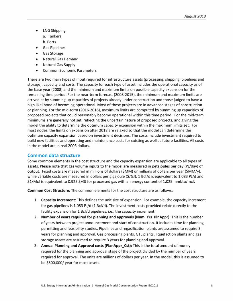
• LNG Shipping a. Tankers b. Ports
• Gas Pipelines • Gas Storage • Natural Gas Demand • Natural Gas Supply • Common Economic Parameters
There are two main types of input required for infrastructure assets (processing, shipping, pipelines and storage): capacity and costs. The capacity for each type of asset includes the operational capacity as of the base year (2008) and the minimum and maximum limits on possible capacity expansion for the remaining time period. For the near-term forecast (2008-2015), the minimum and maximum limits are arrived at by summing up capacities of projects already under construction and those judged to have a high likelihood of becoming operational. Most of these projects are in advanced stages of construction or planning. For the mid-term (2016-2018), maximum limits are computed by summing up capacities of proposed projects that could reasonably become operational within this time period. For the mid-term, minimums are generally not set, reflecting the uncertain nature of proposed projects, and giving the model the ability to determine the optimum capacity expansion within the maximum limits set. For most nodes, the limits on expansion after 2018 are relaxed so that the model can determine the optimum capacity expansion based on investment decisions. The costs include investment required to build new facilities and operating and maintenance costs for existing as well as future facilities. All costs in the model are in real 2006 dollars.
Common data structure Some common elements in the cost structure and the capacity expansion are applicable to all types of assets. Please note that gas volume inputs to the model are measured in petajoules per day (PJ/day) of output. Fixed costs are measured in millions of dollars ($MM) or millions of dollars per year ($MM/y), while variable costs are measured in dollars per gigajoule ($/GJ). 1 Bcf/d is equivalent to 1.083 PJ/d and $1/Mcf is equivalent to 0.923 $/GJ for processed gas with an energy content of 1.025 mmbtu/mcf.
Common Cost Structure: The common elements for the cost structure are as follows:
1. Capacity Increment: This defines the unit size of expansion. For example, the capacity increment for gas pipelines is 1.083 PJ/d (1 Bcf/d). The investment costs provided relate directly to the facility expansion for 1 Bcf/d pipelines, i.e., the capacity increment.
2. Number of years required for planning and approvals (Num_Yrs_PlnAppr): This is the number of years between project announcement and start of construction. It includes time for planning, permitting and feasibility studies. Pipelines and regasification plants are assumed to require 3 years for planning and approval. Gas processing plants, GTL plants, liquefaction plants and gas storage assets are assumed to require 3 years for planning and approval.
3. Annual Planning and Approval costs (PlanAppr_Cst): This is the total amount of money required for the planning and approval stage of the project divided by the number of years required for approval. The units are millions of dollars per year. In the model, this is assumed to be $500,000/ year for most assets.

August 2013
U.S. Energy Information Administration | Natural Gas Model Documentation Report IEO2011 9
4. Number of years required for construction (Num_Yrs_Inv): This is the number of years required for construction. In the model, the default assumption for this category is 3 years. The exceptions are small LNG carriers (2 years).
5. Investment cost in year (Investment_Cost): This is the total amount of investment required for construction divided by the number of years required for construction. The units are million dollars per year.
6. Maximum operating life of asset (Maximum_Life): The physical life of an asset before retirement. The current version of the model assumes that all assets have 100 years of physical life. This means that assets will not retire during the model time frame.
7. Annual fixed operating and maintenance costs (Fixed_OaM_Cost): This is the fixed annual operating cost of an asset including taxes, insurance, labor costs etc. This does not include the capital recovery or depreciation cost, which is accounted for separately by the model using the discount rates. The units are millions of dollars per year for an asset of the size specified by the capacity increment.
8. Variable Operating and Maintenance Cost (Variable_OaM_Cost): This is the variable operating and maintenance cost of running an asset and is specified in dollars per gigajoule. It primarily consists of the non-fuel costs associated with operations since fuel costs are captured as part of the fuel use for asset (e.g., pipelines and storage) or in the input and output energy specifications (e.g., processing assets). In one case, tankers, this number includes the cost of the fuel used to run the tankers.
9. Cost of retiring the asset (Retirement_Cost): This represents the cost of retiring an asset and is specified in millions of dollars for an asset of the size specified by the capacity increment. The default assumption used in the model is 0.1 $MM.
Common structure for the asset capacity specification: Once the capacity in the base year is specified, lower and upper bounds on the capacity for the future years are computed by adding the minimum and maximum volume of capacity expansion that can occur. As explained earlier, projects already under construction or in advanced stages of planning are assumed to definitely become operational and their capacities are used as the minimum capacity expansion for that node. The minimum capacity limits are usually set for projects becoming operational in the 2008-2015 timeframe. Once an expansion is announced, the asset will go through the planning and construction phases based on the number of years specified (Num_Yrs_PlnAppr, Num_Yrs_Inv). The capacity expansion from year 2008 (base year) till 2015 is constrained based on the announcements already made in the media. From 2016 onwards, the minimum capacity expansion is generally set at zero. From 2016 to 2018 maximum capacity expansions are set based on proposed projects, and beyond 2018 the maximums are set at 99999 PJ/d (except where we have limited it to keep the model from building capacities to unrealistic levels), an artificially high number that indicates that the model can build new capacity as required based on investment decisions. The following are elements of the common structure used to specify asset capacities in the model:
1. Node Name (NodeId): Node for which the capacity is specified. 2. Asset Id (AssetId): The asset within the node for which the capacity is specified (e.g. GTL
Plant, Liquefaction facility etc.)

August 2013
U.S. Energy Information Administration | Natural Gas Model Documentation Report IEO2011 10
3. Start Year (SYear): First year that following data apply for (e.g., 2008) 4. Last Year (EYear): Last year that following data apply for (e.g., 2008) 5. Minimum Capacity (Min_Capacity): Minimum capacity expansion allowed in the region. The
units are PJ/day output of primary fuel. 6. Maximum Capacity (Max_Capacity): Maximum capacity expansion allowed in the region.
The units are PJ/day output of primary fuel.
The next section gives the numeric values for the cost and capacity parameters used in the model and the underlying assumptions/sources.

August 2013
U.S. Energy Information Administration | Natural Gas Model Documentation Report IEO2011 11
Model Assumptions for Individual Asset Categories
1. Processing assets
Asset capacity The capacity assumptions for all liquefaction, regasification, and GTL plants are provided in Appendix B, Table B.1. The gas processing capacity is assumed to be unconstrained.
Asset Costs and Energy Conversion Specifications
Table A.1 and Table A.2 in Appendix A provides the specifications for the different processing [1, 2, 3], liquefaction [4, 5, 6], regasification [4, 5, 7], and GTL plants [8, 9].
Note that industry estimates put the overall energy efficiency for the GTL process at about 60% (i.e., for 100 Btu of natural gas in, you get about 60 Btu of hydrocarbon product out) [10]. In newer plants, it appears to require about 10 MMBtu of gas to produce one barrel of GTL product. Energy efficiency is more consistently cited at about 65%, .i.e., the energy content of the GTL product represents only 65% of what was contained in the input gas [11].
2. LNG shipping
Tanker capacity Table B.2 in Appendix B provides the assumed LNG shipping capacity. A database of existing LNG carriers and those on order was built using the data available on the Maritime Business Strategies, LLC website [12]. Existing ships have a capacity of about 135,000 cu.m with a few ships below the 100,000 cu.m size. The ships that are on order range from 135,000 cu.m to 270,000 cu.m (ordered by RasGas, Qatar) in capacity. Based on the data, four ship categories were defined: Small (<100,000 cu. m. LNG), Medium (100,000-160,000), Large (160,000-200,000) and Ultra-Large (>200,000). Next, the delivery date for each ship was used to determine if the ship was an existing ship, or an ordered ship. Since the model base year is 2008, all ships delivered after 2008 have been moved to the “ordered” category which is essentially the number of LNG ships forecasted. The forecast is limited to 2008-2010 because that is the extent of the Colton database. For 2008 to 2010, ICF forecasted for each year the number of ships in each size class added to the LNG fleet. Between 2008 and 2010, ICF assumed no growth in the number of ships beyond those listed as ordered in the Maritime Business Strategies, LLC database. After 2010, ICF allowed the model to decide on new ship construction based on requirements. The short term forecast was validated by comparing against predictions by other sources. One such source was the website of Mitsui O.S.K. Lines that owns nearly one-quarter of the world LNG shipping fleet [13]. As of 12/1/2006, the website indicated that there will be a total of 344 LNG ships by 2010. This compares well with the 335 ships that we have in the INGM database based on data from Maritime Business Strategies, LLC.
The majority of ships that are on order fall into the medium capacity category of 100,000-160,000 cu. m. LNG. Some ships that are scheduled to be delivered after 2006 will have very large capacities not seen in the existing fleet.

August 2013
U.S. Energy Information Administration | Natural Gas Model Documentation Report IEO2011 12
Tanker costs The tanker cost and other specifications are provided in Table A.3 of Appendix A.
The Maritime Business Strategies, LLC database also has values for the construction cost of most ships on order and we estimated the tanker costs using this data. The medium and large tanker costs are set consistent with the average costs for ships of that size and costs for the small and ultra-large tankers are estimated using a linear extrapolation from these values1 .
Average ship speed Based on the fleet data, the design speed for new LNG carriers is approximately 19.5 knots. The average ship speed on port to port voyages was assumed to be 80% of the design speed to account for slow speeds due to port manoeuvring and bad weather. Other related data sources for LNG carriers are [15, 5, 12].
Ports and routes Each node was assigned a port city that was used to calculate distances between ports. Port cities were selected based on existing, planned or proposed LNG infrastructure or based on ICF assessment of the most logical LNG port for a given node.
Each node was assigned one port to be used in estimating distance between nodes. Port distances were taken from a distance calculator ‘Sea Distances - Voyage Calculator’ [16]. For links where the distance could be reduced by using the Suez Canal, it was assumed that the ship would pass through it, and the reduced distance was estimated. The number of days required by tankers to complete a one-way journey on each link was estimated by dividing the total distance by an average tanker speed of 80% of 19.5 knots for all tanker categories.
ICF assessed a matrix of exporting and importing nodes to determine the most likely routes for LNG trade. ICF used knowledge of LNG market supply and demand to populate the model with likely LNG trade routes rather than all possible node to node connections.
The utilization of either the Panama or Suez Canal was determined by the Sea Distance and Voyage Calculator. A ship that travels through one of these canals incurs tolls not paid by other LNG ships. Therefore, on any route through a canal an additional cost had to be calculated and applied to the total shipping cost for that route.2
The Suez Canal cost was calculated using the Suez Toll Calculator [17], which requires inputs to determine the tolls for an LNG tanker. The following LNG tanker assumptions were made to calculate the total canal charge: capacity- 160,000 cubic meters, Suez specific tonnage- 105,000 dwt, gross laden part and ballast legs of the trip and added together to determine a total roundtrip canal cost. LNG tankers going through the Suez Canal receive a 35% rebate, which was applied to the total cost. The final total cost after the rebate was divided by the volume of gas aboard the ship to arrive at the cost in $/GJ.
The Panama Canal did not have a toll calculator similar to the Suez toll calculator. To estimate cost, actual 2005 Panama Canal traffic data was used [18]. As for the Suez tolls, both laden and ballast tolls were calculated. The total number of laden trips through the canal was divided by the total tolls 1 LNG carrier Cost data was obtained from [12]. GDP Deflator was estimated from Bureau of Economic Analysis data Current-Dollar and "Real" Gross Domestic Product [14]. 2 The canal tolls have not yet been implemented.

August 2013
U.S. Energy Information Administration | Natural Gas Model Documentation Report IEO2011 13
collected to calculate an average toll per ship. The same was done for ballast trips. Average laden ship tolls were added to average ballast ship tolls for a total Panama Canal toll cost. The final total cost was divided by the volume of gas aboard the ship to arrive at the cost in $/GJ.
3. Gas pipelines
Pipeline capacity Appendix B, Table B.3 shows the pipeline capacity constraints assumed for the INGM.
ICF forecasted worldwide pipeline capacity based on numerous sources of data. The 2008 base year data for North American capacity as well as other international pipeline capacity was supplied by EIA databases. Each pipeline record in the EIA databases had the following properties listed: start point, end point, pipeline name, status, start year, and capacity.
EIA assigned each pipeline in their database a status: operating, under construction, firm, planned, and potential. All five of these statuses were included in the INGM pipeline database. The status represents the likelihood that the pipeline will at some point be completed and additional capacity added. The pipelines with a status of operating were included in the base capacity estimate. The scale for likelihood of completion went from “under construction” (the most likely) to “potential” (the least likely).
Existing gas pipeline capacity data were collected for the U.S.A [19], Europe [20], Russia [21], as well as for other regions [22]. Capacity expansion data was obtained from EIA [23, 24] and ICF’s internal data sources.
Pipeline costs and specifications Appendix A, Table A.4 shows the assumptions for the pipeline asset costs. The standard unit of pipeline expansion (capacity increment) was assumed to be 1 Bcf/d. The cost of expansion between different nodes is estimated using the distance between two representative locations in those nodes. Pipeline investment costs were calculated using data from an Oil & Gas Journal survey, which reported the actual total costs and distances for fifteen pipelines built in the United States in 2005. ICF used pipeline diameter to calculate the daily pipeline flow rate. ICF then divided the total reported cost by the flow rate to calculate the average dollars per mile per Bcf of gas flow per day for the fifteen pipelines in the survey. This average, $2.8 million per mile per Bcf/d3 , was applied to each pipeline link represented in the INGM to calculate total investment costs based on distance. Because the number of years for investment (3 years) and the unit of expansion (1 Bcf/d) are constants, total pipeline investment cost for different links varies based solely on distance.
Variable operating and maintenance pipeline costs are based on fuel use and gas price consistent with [25, 26]. ICF used fuel use data for an upcoming pipeline being built from the Rocky Mountains to Ohio as the default for all pipeline links. The ‘Rockies Express’ pipeline project fuel usage percentage is equivalent to 2.59% per 1000 miles of pipeline length. Variable O&M costs were then calculated by multiplying the fuel use by an ICF assumed gas price of $5/GJ.
3 The exception to this rule are the pipelines originating in the Russia Arctic node. Due to the inhospitable construction and operating environment, the unit capital cost was doubled for pipelines connecting Russia Arctic to Russia West and Russia East.

August 2013
U.S. Energy Information Administration | Natural Gas Model Documentation Report IEO2011 14
Pipelines from the ‘Russia Arctic’ nodes. The nodes in the Russian Arctic region (above the Arctic Circle) contain some of the largest Russian gas resources. The resources in this node were discovered nearly two decades ago and are counted as reserves; however there is no current production as political decisions have regularly delayed investment in production facilities. The Russian state natural gas company, Gazprom indicates that the resources in these nodes will be home to the biggest new production developments that will constitute most of the expected increase in Russia’s natural gas supply over the next three decades. The key developments include Shtokman and the Yamal Peninsula (onshore and offshore) which have been in the news for many years and are currently expected to start producing in the next 10 to 20 years.
Due to the special nature of this supply reserve, production from it cannot be predicted based on economics alone. The pipeline capacity and marine LNG links that will take gas out of this region are used to model the above-ground constraints on supply. The pipelines connecting to the Russian arctic nodes have artificial capacity constraints which have been applied to approximate the production schedule as per official announcements and analyst judgement.
4. Gas storage Gas storage in the INGM only covers underground storage facilities that can be used for seasonal storage of natural gas. Small gas storage facilities at LNG plants or other facilities that are used for operational smoothing are not included in this category. The list of existing gas storage facilities is taken from the CEDIGAZ Underground Gas Storage in the World 2006 report.
Gas storage capacity constraints Appendix B, Table B.4 contains the assumed constraints for gas storage capacity. The primary source of data on existing working gas storage capacity was obtained from a CEDIGAZ publication [27] that lists underground natural gas storage capacity in the world, by country, as of January 2006.
ICF used data from the EIA [28] to allocate the United States capacity as reported by CEDIGAZ to the various United States INGM regions.
Outside the U.S., EIA made the following assumptions regarding countries with storage capacity that have more than one node:
• All existing Canadian capacity is in the Canada East node • All Australia capacity is in the Australia and NZ Demand node • All Russia capacity is in the Russia West node • All China capacity is in the Northeast China node
August 2013
U.S. Energy Information Administration | Natural Gas Model Documentation Report IEO2011 15
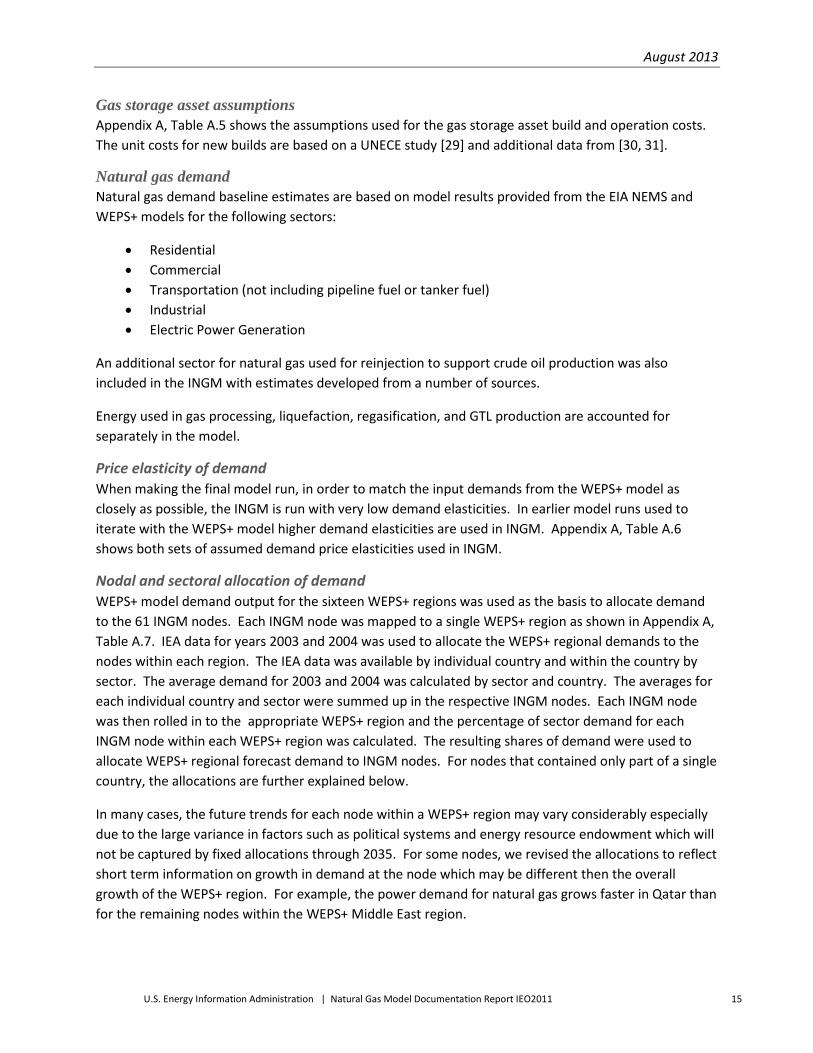
Gas storage asset assumptions Appendix A, Table A.5 shows the assumptions used for the gas storage asset build and operation costs. The unit costs for new builds are based on a UNECE study [29] and additional data from [30, 31].
Natural gas demand Natural gas demand baseline estimates are based on model results provided from the EIA NEMS and WEPS+ models for the following sectors:
• Residential • Commercial • Transportation (not including pipeline fuel or tanker fuel) • Industrial • Electric Power Generation
An additional sector for natural gas used for reinjection to support crude oil production was also included in the INGM with estimates developed from a number of sources.
Energy used in gas processing, liquefaction, regasification, and GTL production are accounted for separately in the model.
Price elasticity of demand When making the final model run, in order to match the input demands from the WEPS+ model as closely as possible, the INGM is run with very low demand elasticities. In earlier model runs used to iterate with the WEPS+ model higher demand elasticities are used in INGM. Appendix A, Table A.6 shows both sets of assumed demand price elasticities used in INGM.
Nodal and sectoral allocation of demand WEPS+ model demand output for the sixteen WEPS+ regions was used as the basis to allocate demand to the 61 INGM nodes. Each INGM node was mapped to a single WEPS+ region as shown in Appendix A, Table A.7. IEA data for years 2003 and 2004 was used to allocate the WEPS+ regional demands to the nodes within each region. The IEA data was available by individual country and within the country by sector. The average demand for 2003 and 2004 was calculated by sector and country. The averages for each individual country and sector were summed up in the respective INGM nodes. Each INGM node was then rolled in to the appropriate WEPS+ region and the percentage of sector demand for each INGM node within each WEPS+ region was calculated. The resulting shares of demand were used to allocate WEPS+ regional forecast demand to INGM nodes. For nodes that contained only part of a single country, the allocations are further explained below.
In many cases, the future trends for each node within a WEPS+ region may vary considerably especially due to the large variance in factors such as political systems and energy resource endowment which will not be captured by fixed allocations through 2035. For some nodes, we revised the allocations to reflect short term information on growth in demand at the node which may be different then the overall growth of the WEPS+ region. For example, the power demand for natural gas grows faster in Qatar than for the remaining nodes within the WEPS+ Middle East region.

August 2013
U.S. Energy Information Administration | Natural Gas Model Documentation Report IEO2011 16
The allocations by sector are based on historical IEA energy balance data. The 2004 edition of IEA energy balance was used, which included time series data for all countries through 2002. Table 1 details how energy flows in the IEA data were classified into sectors for the model and coefficients assigned to the flows for the purpose of aggregating them into the INGM sectors.
Table 1. Classification of IEA energy flows to INGM sectors
IEA Flow INGM Sector Coefficient
International Marine Bunkers Transportation -1
Public Electricity Plants Electric Power -1
Autoproducer Electricity Plants Electric Power -1
Public CHP Plants Electric Power -1
Autoproducer CHP Plants Industrial Cogen -1
Public Heat Plants Commercial -1
Autoproducer Heat Plants Industrial Heat/fuel Usage -1
Petroleum Refineries Industrial Feedstock 0
Coal Transformation Industrial Feedstock 0
Other Transformation Industrial Feedstock 0
Own Use Own Use/Lease and Plant Fuel -1
Distribution Losses Residential 0
Iron and Steel Industrial Heat/Fuel Usage 1
Chemical and Petrochemical Industrial Heat/Fuel Usage 1
Memo: Feedstock Use in Petchem. Industry Industrial Feedstock 1
Non-ferrous Metals Industrial Heat/Fuel Usage 1
Non-Metallic Minerals Industrial Heat/Fuel Usage 1
Transpoort Equipment Industrial Heat/Fuel Usage 1
Machinery Industrial Heat/Fuel Usage 1
Mining and Quarrying Industrial Heat/Fuel Usage 1
Food and Tobacco Industrial Heat/Fuel Usage 1
Paper, Pulp and Printing Industrial Heat/Fuel Usage 1
Wood and Wood Products Industrial Heat/Fuel Usage 1
Construction Industrial Heat/Fuel Usage 1
Textile and Leather Industrial Heat/Fuel Usage 1
Non-specified Industry Industrial Heat/Fuel Usage 1
International Civil Aviation Transportation 1
Domestic Air Transport Transportation 1
Road Transportation 1
Rail Transportation 1

August 2013
U.S. Energy Information Administration | Natural Gas Model Documentation Report IEO2011 17
Table 1. Classification of IEA energy flows to INGM sectors (cont.)
IEA Flow INGM Sector Coefficient
Pipeline Transport Pipeline Fuel 1
Internal Navigation Transportation 1
Non-specified Transport Transportation 1
Agriculture Industrial Heat/Fuel Usage 1
Commercial and Public Services Commercial 1
Residential Residential 1
Non-specified Other Commercial 1
Non-Energy Use Ind/Transf/Energy Industrial Feedstock 1
Non-Energy Use in Transport Transportation 1
Non-Energy Use in Other Sectors Industrial Feedstock 1
TPES Minus TFC Transformation 1
The following combinations of fuels and flows have coefficients of zero, superseding those listed above:
• Electricity: All three types autoproducer plants, all three types public plants • Heat: All three types autoproducer plants, all three types public plants • Crude, NGL and Feedstocks: Other Transformation
The "Chemical and Petrochemical" values used are derived by subtracting "Memo: Feedstock Use In Petchem. Industry" values from the IEA data values for "Chemical and Petrochemical."
Countries that came into existence during the period covered by the IEA time series necessitated two assumptions for the purpose of generating continuous time series:
• For former Soviet republics: 1971-1991 demand data for each of the 15 member republics were computed as a percentage of the "Former USSR" totals. A separate percentage was computed for each fuel and sector combination using 1992 numbers.
• For the former Yugoslavia: Since all the current states of the former Yugoslavia are in the same INGM node, demand data for "Former Yugoslavia" was retained instead of computing estimates for each of the current states for the period prior to the dissolution.
Sub-country allocation There are six countries that each comprises two or more INGM nodes, thus requiring national-level consumption figures to be allocated to the nodes. Similar but not identical methodologies were used for the allocation based on relevant information that was available. In general, subnational proportions were calculated and applied to all previous years of historical data.
United States: The United States demand projections for the nine census divisions were allocated to INGM nodes based on EIA’s state-level natural gas consumption data for 2003 through 2007 [32].

August 2013
U.S. Energy Information Administration | Natural Gas Model Documentation Report IEO2011 18
Canada: Canada’s national-level demand was allocated to INGM nodes based on the sum of 2002 Statistics Canada data for direct sales and utility sales, as follows [33]:
Canada East - 43.8% Canada West - 56.2%
Mexico: Mexico’s national-level demand was allocated to INGM nodes as follows [34]:
Mexico Northwest - 5.2% Mexico Northeast - 25.7% Mexico South - 69.1%
India: India’s national-level demand was allocated to INGM nodes by population, as follows [35]:
India - North - 48% India – Southeast - 29% India - Southwest - 23%
China: China’s national-level demand was allocated to INGM nodes as follows [36]:
China - West - 28% China - Northeast - 31% China - South - 41%
Russia: Russia’s national-level demand was allocated to INGM nodes as follows [37]:
Russia West - 90% Russia East - 10%
This allocation is based on a Gazprom report stating that 34% of 2006 domestic consumption took place in the Central Federal District, 14% in the Southern Federal District, and 32% in the Volga Federal District. All the consumption for these three districts is included in the Russia West node, as well as for two of the four remaining districts. The remaining 20% of consumption is allocated to the remaining four federal districts by population.
Australia: Australia’s national-level demand was allocated to INGM nodes consistent with the historic demand in Western Australia verses that in Eastern Australia and New Zealand as follows:
Australia and New Zealand - Demand - 70.3% Australia and New Zealand - NW Shelf - 29.7%
Seasonal multipliers by sector Seasonal multipliers were calculated for INGM nodes and sectors. These multipliers are applied to annual base demand numbers to model seasonal variation in natural gas demand by sector. The following two sections describe how seasonal multipliers were calculated for the 61 INGM nodes.

August 2013
U.S. Energy Information Administration | Natural Gas Model Documentation Report IEO2011 19
United States: Monthly data from 2001-2005 for each sector [38] was used to calculate average monthly consumption on an MMcf/d basis for the United States as a whole. The months were then broken down in to seasons as follows: December, January and February constitute Winter; June, July, August constitute Summer; and March, April, May, September, October, November constitute Spring/Fall. The average seasonal consumption on an MMcf/d basis was calculated for each season. The seasonal multipliers were then calculated by dividing the average seasonal consumption by the average annual consumption.
Japan: The electric power sector accounts for nearly two-thirds of the annual gas consumption in Japan. Seasonal multipliers for the Japanese electric power sector were derived from monthly “Electricity Generated and Purchased” bulletins from the Federation of Electric Power Companies of Japan [39]. These bulletins list the monthly gas purchase and consumption for electricity generation.
The seasonal demand pattern for the other sectors in Japan was estimated using the same method as for “Other Nodes” given below.
South Korea: Monthly gas consumption statistics for South Korea were obtained from the Korea Energy Economics Institute [40]. The data from this website was used to develop seasonal allocation factors for the Electric, Residential/Commercial and Industrial sectors.
Europe: Monthly gas consumption statistics for European countries was obtained from the Eurostat database [41]. The data for the individual countries was aggregated to IEO regions (OECD Europe and Non-OECD Europe). The monthly statistics were available for two broad categories in each region: Power Generation Sector and Gross Inland Consumption. The seasonal multipliers derived from Eurostat’s power generation sector were applied to the Power Generation Sector of INGM for OECD Europe and Non-OECD Europe regions respectively, and multipliers derived from gross inland consumption were applied to all other sectors in OECD Europe, and Non-OECD Europe.
Other Nodes: A different method was used for regions for which monthly or quarterly data were unavailable. The other regions that have seasonal differences in demand are: Arabian Producers, Australia and New Zealand, Brazil, Canada, Chile, China, FSU Central Asia, India, Iran, Latin America – Southern Cone, Qatar, Russia, and Saudi Arabia. The four sectors that may have seasonal differences are: Residential, Commercial, Industry, and Power Generation. Not all nodes have seasonal variation in all sectors. For instance, Saudi Arabia only has seasonal differences only in the power generation sector.
To estimate the seasonal variation in these regions and sectors, ICF matched the regions with U.S. regions based on weather data. ICF used a climate database with heating degree day (HDD) and cooling degree day (CDD) data for weather stations all over the world. For each region, a weather station was chosen that was as close as possible to a primary demand center in that region based on longitude and latitude coordinates. The average HDD and CDD were calculated for that weather station. ICF then performed an analysis of U.S. weather stations to examine which U.S. weather stations have a similar weather pattern to the foreign region station based on HDD and CDD. For each region, two U.S. weather stations were chosen that exhibited very similar HDD and CDD data. The corresponding EIA monthly state and sector-level data [38] for each U.S. weather station was used to calculate the seasonality for each region as described in the U.S. methodology above.
For the remaining regions, ICF assumed no seasonality in demand, based on knowledge of the climate and natural gas demand.

August 2013
U.S. Energy Information Administration | Natural Gas Model Documentation Report IEO2011 20
Nodal allocation of wholesale prices WEPS+ model wholesale prices for the 16 WEPS+ regions was used as the basis to allocate prices to the 61 INGM nodes. Each INGM node was mapped to a single WEPS+ region as shown in Appendix A, Table A.7. The WEPS+ regional wholesale price was allocated to component nodes based on nodal prices from the previous INGM run.
Natural gas resources and extraction This section provides an overview of the data sources used to estimate natural gas resources and extraction and details how the resource estimates are used to produce resource extraction curves for use in the INGM.
Conventional gas resources: The primary data source was the United States Geological Survey (USGS), which provides data on gas resources for the United States [42, 43] and the world [44]. The USGS data include the following:
• Resource data by assessment units (AU) (306 globally) • A field size distribution for the remaining resources in each AU, • Mean resources for each AU, • Minimum, median, and maximum well depths for each AU, • Minimum, median, and maximum water depths for each AU. • The portion of resources that are onshore and offshore
Canada conventional gas resources The 2000 USGS assessment only covered some areas of Canada. In order to include a comprehensive assessment of the remaining Canadian potential, ICF developed an analysis that combines the recent USGS assessment of the Mackenzie –Beaufort region and a previous analysis carried out in 2003 by the National Petroleum Council, an industry sponsored forecasting analysis of North American gas markets which includes detailed oil and gas resource base characterization of the U.S., Canada, and Mexico [45]. This new analysis includes the Western Canadian Sedimentary Basin, the East Coast onshore and offshore, and various frontier regions of Canada. For each area, a field size distribution was specified, as was the mix of crude oil, natural gas, and NGLs. ICF also included estimates of onshore drilling depth and offshore water depth for each area. Proved reserves in Canada are provided in [46].
China conventional gas resources The 2000 USGS assessment covered the undiscovered resources and field size distribution of major future potential areas for China. More recent data on oil and gas reserves were also available [47, 48]. For the INGM, it was necessary to re-allocate the USGS resources in China to the three INGM nodes for China. ICF evaluated the map distribution of the USGS basin assessments to assign resources to specific nodes.

August 2013
U.S. Energy Information Administration | Natural Gas Model Documentation Report IEO2011 21
Conventional gas reserves growth The 2000 USGS assessment also provides AU level data on the growth of gas volume from the non-U.S. gas and oil fields. This data is used in INGM to estimate reserves growth (RG) for each AU. The AU level reserve growth is calculated based on AU level growth volumes, reserves, and estimated ultimate recovery (EUR), and is scaled up to meet the world growth target (excluding U.S.) of 3,305 Tcf. The following is the procedure for calculating an AU-level reserves growth factor:
1. Start with USGS growth volumes by AU 2. Scale up the growth volume to reach the world growth target (excluding US) of 3,305 Tcf subject to:
a. Minimum growth of 30% of AU reserves
b. Maximum growth of 75% of AU estimated ultimate recovery (EUR)
3. Calculate RG factor:
AU RG Factor = ( [AU Resources] + [AU Growth] ) / [AU Resources]
Since basin level growth data is not available for the United States, a constant RG percentage is assumed for U.S. regions. Values of 1.9157 and 1.72 are used for U.S. onshore and offshore regions, respectively.
Unconventional gas resources Multiple data sources and documents were used to estimate unconventional gas resources [49, 50, 51, 52, 53].
[49] provides worldwide estimates of gas-in-place for coalbed methane, shale gas, and tight-sand gas resources (Table 2). The article further mentions that the volume of undiscovered resources is around 10% of the total gas-in-place for the United States. But more recent estimates of recoverable reserves suggest a ratio of closer to 19% which we used to estimate the economically and technically recoverable resources for tight gas, shale gas and coal bed methane (CBM).

August 2013
U.S. Energy Information Administration | Natural Gas Model Documentation Report IEO2011 22
Table 2. Total undiscovered unconventional in-place gas resources4
Coalbed Methane Shale Gas
Tight-Sand
Gas Total
Region Tcf Tcf Tcf Tcf
North America 3,017 3,840 1,370 8,228
Latin America 39 2,116 1,293 3,448
Western Europe 157 509 353 1,019
Central and Eastern Europe 118 39 78 235
Former Soviet Union 3,957 627 901 5,485
Middle East and North Africa 0 2,547 823 3,370
Sub-Saharan Africa 39 274 784 1,097
Centrally planned Asia and China 1,215 3,526 353 5,094
Pacific OECD 470 2,312 705 3,487
Other Asia Pacific 0 313 549 862
South Asia 39 0 196 235
World 9,051 16,103 7,406 32,560
The regional estimates of reserves and undiscovered resources are presented in Figure and Figure below. The allocation of natural gas between reserves and undiscovered resources differs from the allocation based on USGS data, due to the reallocation in regions with P/R ratios less than 0.04. In this case, some of the reserves are modelled as very low cost undiscovered resources. The regional allocation also reflects modifications to reserves and resources in Canada and China.
Figure 1. Reserves in the INGM 5
EJ
4 [49, 50] 5 Existing reserves of unconventional gas may be classified as conventional where no separate data exists.
0100200300400500600700
Conventional Offshore Conventional Onshore CoalBed Methane Shale Gas Tight Gas

August 2013
U.S. Energy Information Administration | Natural Gas Model Documentation Report IEO2011 23
Figure 2. Undiscovered Resources in the INGM EJ
Resource extraction cost curves In order to develop resource extraction cost curves, ICF used average nodal field size distributions and well depths from USGS conventional resources.
The aforementioned data sources provide resource estimates but do not provide the cost of developing and producing the resources with one exception, the MMS source for offshore federal resources in the United States. ICF then integrated these estimates within a simplified development/production cost model to develop resource extraction curves.
The resource cost curves were developed as follows:
• Allocate resources to resource steps based on field size classes, well depths, and water depths • Determine the number of wells for each resource step based on the field size • Determine the production to reserves ratio based on field size • Determine development and operating costs for the resource step • Estimate minimum acceptable supply price for the resource step • Convert the field size class resource step into a risk-based drilling step using the field find rate
matrix which was developed from ICF’s World Assessment Unit (WAU) model
Resource steps: The allocation of undiscovered resources to the resource step first involves allocating the resources to field size categories based on the field size distribution. In many cases, the sum of the fields in each field size category times the average resources in the field size category do not add to the estimated mean resources. The number of fields is then scaled to achieve this.
Number of wells per field: The number of wells per field is determined by the following formula that was derived from a more detailed production model (ICF’s North American Natural Gas Analysis System – NANGAS) for the United States and constrained to reflect the much larger fields in the Middle East, and Russia.
0
1000
2000
3000
4000
5000
6000Conventional Offshore Conventional Onshore CoalBed Methane Shale Gas Tight Gas

August 2013
U.S. Energy Information Administration | Natural Gas Model Documentation Report IEO2011 24
𝑁𝑊𝑒𝑙𝑙𝑠𝑟𝑠 =𝑀𝑖𝑛[𝐸𝑋𝑃(𝑁𝑊𝐼 + 𝑁𝑊𝑅𝑒𝑠 ∗ log(𝑅𝑒𝑠𝑟𝑠) +𝑈𝑛𝑊𝑙𝐴𝑟𝑠) ∗ 5,𝑀𝐴𝑋 � RESrs
MnWellrs, EXP(NWI +
NWRes ∗ log( Resrs) + UnW1Ars)�]
NWellsrs = MIN(EXP(NWI+NWRes*Log(Resrs)+UnWlArs) *5,
MAX(Resrs /MnWellrs),EXP(NWI+NWRes*Log(Resrs)+UnWlArs))
where,
• NWellsrs is the number of wells estimated for each field in the field size class • Resrs is the average size of the field size class (Bcf) • MnWellrs is the minimum number of wells needed to develop the field size class. The values of
6.5 for conventional and 3.5 for unconventional resources are utilized based on regression analysis of U.S. resources using NANGAS model
• NWI and NWRes are regression coefficients derived from the same regression above which take the values 1.446804 and 0.417948 respectively
• UnWlArs is an adjustment for unconventional resources which take the value 1.157944 for coalbed methane and shale gas, and 0.628118 for tight gas and is derived from the same regression above
PR ratio: The production to reserves ratio is then estimated. The first step is to estimate the present value of production for the field size class based on the following equation:
𝑃𝑉𝑃𝑟𝑑𝑟𝑠 = 𝐸𝑋𝑃(−0.57965 + 0.965089 ∗ log(𝑅𝑒𝑠𝑟𝑠))
where,
• PVPrdrs is the present value of production from the field (BCF), and • the two coefficients are estimated using regression analysis of NANGAS results on multiple
fields in the United States. This estimate of present value of production assumes a real discount rate of 12%.
The PR ratio is then estimated from the reserves in the field and the present value of reserves as follows:
𝑃𝑅𝑟𝑠 = �𝑃𝑉𝑃𝑟𝑑𝑟𝑠𝑅𝑒𝑠𝑟𝑠
� ∗ (1 − 0.9)/(1 − �𝑃𝑉𝑃𝑟𝑑𝑟𝑠𝑅𝑒𝑠𝑟𝑠
� ∗ 0.9)
where,
• PRrs is the production to reserves ratio (fraction).

August 2013
U.S. Energy Information Administration | Natural Gas Model Documentation Report IEO2011 25
Drilling costs : The next step is to estimate drilling costs using the equation below:
𝐷𝐷𝐶𝑠𝑡𝑟𝑠 = 1.1542∗ �(𝑑𝑐1 + 𝑑𝑐2 ∗ 𝐷𝐷𝑟𝑠 + 𝑑𝑐3 ∗ 𝐷𝐷𝑟𝑠2 + 𝑑𝑐4 ∗ 𝐷𝐷𝑟𝑠3 ) ∗ 1.1
+ (0.000079863 ∗ 𝐷𝐷𝑟𝑠 ∗ 𝑊𝐷𝑟𝑠)� ∗ �𝑁𝑊𝑒𝑙𝑙𝑠𝑟𝑠𝐷𝑆𝑢𝑐𝑅𝑎𝑡𝑒
− 1� ∗ 𝐷𝐶𝑜𝑠𝑡𝑆𝑟𝑠
𝐸𝐷𝐶𝑠𝑡𝑟𝑠 = 1.1542∗ �(𝑑𝑐1 + 𝑑𝑐2 ∗ 𝐷𝐷𝑟𝑠 + 𝑑𝑐3 ∗ 𝐷𝐷𝑟𝑠2 + 𝑑𝑐4 ∗ 𝐷𝐷𝑟𝑠3 ) ∗ 1.1 ∗ 𝑑𝑐5+ (0.000079863 ∗ 𝐷𝐷𝑟𝑠 ∗ 𝑊𝐷𝑟𝑠)� ∗ 𝑁𝑊𝑒𝑙𝑙𝑠𝑟𝑠 ∗ 𝐷𝐶𝑜𝑠𝑡𝑆𝑟𝑠)/𝐸𝑆𝑢𝑐𝑅𝑎𝑡𝑒
where,
• DDCstrs is the development drilling costs ($000) for the field • EDCstrs is the exploration drilling costs ($000) for the field • 1.1542 is inflation adjustment and 1.1 is a drilling cost adjustment, • DDrs is the drilling depth (ft), • WDrs is the water depth (ft), • dc1, dc2, dc3, dc4, and dc5 take the values below
dc1 dc2 dc3 dc4 dc5
203.7943063 0.025909 9.23E-07 5.45E-10 1.324375
• DSucRate is development drilling success rate (fraction) and is set to 0.9 • ESucRate is exploration drilling success rate (fraction) and is set to 0.2 • DCostSrs is set to 1.0 for conventional resources and 1.75 for unconventional resources.
Fixed operating costs: The fixed operating costs are estimated as a function of the number of wells and well depth for onshore resources and as a function of the number of wells for offshore resources as follows:
𝐹𝑜𝑐𝑟𝑠 = 2.37 ∗ 𝑁𝑊𝑒𝑙𝑙𝑠𝑟𝑠 ∗ 𝐷𝐷𝑟𝑠 if the resource is onshore and
𝐹𝑂𝐶𝑟𝑠 = 289423.7 ∗ 𝑁𝑊𝑒𝑙𝑙𝑠𝑟𝑠 otherwise
where,
• FOCrs is the fixed operating costs ($000 per year)
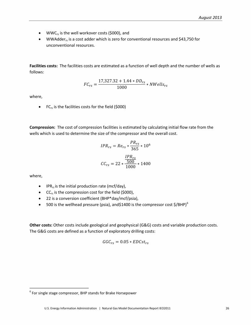
Well workover costs: ICF assumes one workover per well during the production life (10th year) with the following cost structure:
𝑊𝑊𝐶𝑟𝑠 = 25000+3∗𝐷𝐷𝑟𝑠+𝑊𝑊𝐴𝑑𝑑𝑒𝑟𝑟𝑠1000
∗ 𝑁𝑤𝑒𝑙𝑙𝑠𝑟𝑠
where,
August 2013
U.S. Energy Information Administration | Natural Gas Model Documentation Report IEO2011 26
• WWCrs is the well workover costs ($000), and • WWAdderrs is a cost adder which is zero for conventional resources and $43,750 for
unconventional resources.
Facilities costs: The facilities costs are estimated as a function of well depth and the number of wells as follows:
𝐹𝐶𝑟𝑠 =17,327.32 + 1.44 ∗ 𝐷𝐷𝑟𝑠
1000∗ 𝑁𝑊𝑒𝑙𝑙𝑠𝑟𝑠
where,
• FCrs is the facilities costs for the field ($000)
Compression: The cost of compression facilities is estimated by calculating initial flow rate from the wells which is used to determine the size of the compressor and the overall cost.
𝐼𝑃𝑅𝑟𝑠 = 𝑅𝑒𝑟𝑠 ∗𝑃𝑅𝑟𝑠365
∗ 106
𝐶𝐶𝑟𝑠 = 22 ∗𝐼𝑃𝑅𝑟𝑠500
1000∗ 1400
where,
• IPRrs is the initial production rate (mcf/day), • CCrs is the compression cost for the field ($000), • 22 is a conversion coefficient (BHP*day/mcf/psia), • 500 is the wellhead pressure (psia), and$1400 is the compressor cost $/BHP)6
Other costs: Other costs include geological and geophysical (G&G) costs and variable production costs. The G&G costs are defined as a function of exploratory drilling costs:
𝐺𝐺𝐶𝑟𝑠 = 0.05 ∗ 𝐸𝐷𝐶𝑠𝑡𝑟𝑠
6 For single stage compressor, BHP stands for Brake Horsepower

August 2013
U.S. Energy Information Administration | Natural Gas Model Documentation Report IEO2011 27
where,
• GGCrs is the G&G costs ($000) The variable production costs are set to $0.20/mcf.
Minimum acceptable supply price
The minimum acceptable supply price is defined as the cumulative discounted present value of costs divided by the cumulative discounted present value of production. All investment costs are assumed to occur in the first year of production. The fixed operating costs occur annually and the variable operating costs are scaled by production. The well workover costs are assumed to occur in the 10th year of production.
Common economic parameters
Prices for diesel fuel from Gas-to-Liquids facilities are set to a Btu equivalent of crude oil prices.
Risk-based drilling resource steps
In order to account for the risks associated in finding different size fields within the assessment unit, a field find rate is applied to the resource cost curves. ICF’s World Assessment Unit (WAU) model is used to construct a matrix of field find rates by field size class (FSC) and by drilling step as shown in Table 3. The matrix is used to convert the original FSC-based resource steps into risk-based drilling steps where a higher probability of finding is given to the larger fields and vice versa.

August 2013
U.S. Energy Information Administration | Natural Gas Model Documentation Report IEO2011 28
Table 3. Field find rate matrix
FSC 5 6 7 8 9 10 11 12 13 14 15 16 17 18 19 20 21
MMBOE 0.75 1.5 3 6 12 24 48 96 192 384 768 1536 3072 6144 12288 24576 49152
Drilling Step Incremental of Fields Found (fraction)
1 0.0068
0.0096
0.0139
0.0204
0.0302
0.0448
0.0665
0.0985
0.1449
0.2107
0.3009
0.4184
0.5599
0.7116
0.8480
0.9424
0.9868
2 0.0076
0.0107
0.0154
0.0225
0.0329
0.0480
0.0696
0.0993
0.1382
0.1846
0.2320
0.2657
0.2655
0.2173
0.1338
0.0552
0.0131
3 0.0084
0.0119
0.0171
0.0246
0.0356
0.0511
0.0720
0.0986
0.1287
0.1564
0.1701
0.1567
0.1128
0.0563
0.0165
0.0022
0.0001
4 0.0093
0.0131
0.0187
0.0268
0.0383
0.0538
0.0735
0.0960
0.1169
0.1276
0.1181
0.0853
0.0425
0.0122
0.0016
0.0001
0.0000
5 0.0103
0.0145
0.0205
0.0291
0.0408
0.0561
0.0741
0.0919
0.1033
0.1001
0.0773
0.0425
0.0141
0.0022
0.0001
0.0000
0.0000
6 0.0114
0.0159
0.0223
0.0313
0.0432
0.0579
0.0736
0.0861
0.0887
0.0752
0.0475
0.0193
0.0040
0.0003
0.0000
0.0000
0.0000
7 0.0125
0.0173
0.0242
0.0335
0.0454
0.0591
0.0720
0.0790
0.0737
0.0539
0.0273
0.0079
0.0010
0.0000
0.0000
0.0000 -
8 0.0137
0.0188
0.0260
0.0356
0.0473
0.0596
0.0693
0.0708
0.0593
0.0368
0.0145
0.0029
0.0002
0.0000
0.0000
0.0000 -
9 0.0149
0.0204
0.0279
0.0376
0.0488
0.0595
0.0656
0.0618
0.0459
0.0238
0.0071
0.0009
0.0000
0.0000
0.0000 - -
10 0.0162
0.0220
0.0298
0.0395
0.0500
0.0586
0.0609
0.0526
0.0342
0.0145
0.0032
0.0003
0.0000
0.0000
0.0000 - -
11 0.0176
0.0237
0.0317
0.0411
0.0506
0.0569
0.0555
0.0435
0.0244
0.0083
0.0013
0.0001
0.0000
0.0000
0.0000 - -
12 0.0190
0.0254
0.0334
0.0426
0.0508
0.0545
0.0495
0.0348
0.0166
0.0044
0.0005
0.0000
0.0000
0.0000 - - -
13 0.0204
0.0270
0.0351
0.0437
0.0504
0.0514
0.0431
0.0270
0.0108
0.0022
0.0002
0.0000
0.0000
0.0000 - - -
14 0.0219
0.0287
0.0366
0.0445
0.0494
0.0476
0.0367
0.0201
0.0066
0.0010
0.0000
0.0000
0.0000
0.0000 - - -
15 0.0234
0.0303
0.0380
0.0449
0.0479
0.0433
0.0304
0.0145
0.0038
0.0004
0.0000
0.0000
0.0000 - - - -
16 0.0249
0.0318
0.0392
0.0449
0.0457
0.0386
0.0244
0.0099
0.0021
0.0002
0.0000
0.0000
0.0000 - - - -

August 2013
U.S. Energy Information Administration | Natural Gas Model Documentation Report IEO2011 29
Table 3. Field find rate matrix (cont.)
Drilling Step Incremental of Fields Found (Fraction)
17 0.0264
0.0332
0.0400
0.0445
0.0431
0.0338
0.0191
0.0065
0.0010
0.0001
0.0000
0.0000
0.0000 - - - -
18 0.0279
0.0345
0.0407
0.0435
0.0400
0.0288
0.0144
0.0041
0.0005
0.0000
0.0000
0.0000 - - - - -
19 0.0293
0.0357
0.0409
0.0421
0.0365
0.0240
0.0104
0.0024
0.0002
0.0000
0.0000
0.0000 - - - - -
20 0.0307
0.0367
0.0409
0.0403
0.0327
0.0195
0.0073
0.0013
0.0001
0.0000
0.0000
0.0000 - - - - -
21 0.0319
0.0374
0.0404
0.0380
0.0287
0.0154
0.0049
0.0007
0.0000
0.0000
0.0000 - - - - - -
22 0.0331
0.0379
0.0396
0.0354
0.0247
0.0118
0.0031
0.0003
0.0000
0.0000
0.0000 - - - - - -
23 0.0341
0.0381
0.0383
0.0324
0.0208
0.0087
0.0019
0.0002
0.0000
0.0000
0.0000 - - - - - -
24 0.0349
0.0380
0.0367
0.0292
0.0171
0.0062
0.0011
0.0001
0.0000
0.0000
0.0000 - - - - - -
25 0.5137
0.3874
0.2526
0.1321
0.0494
0.0111
0.0012
0.0000
0.0000
0.0000
0.0000 - - - - - -
SUM 1.0000
1.0000
1.0000
1.0000
1.0000
1.0000
1.0000
1.0000
1.0000
1.0000
1.0000
1.0000
1.0000
1.0000
1.0000
1.0000
1.0000
August 2013
U.S. Energy Information Administration | Natural Gas Model Documentation Report IEO2011 30
Resource availability constraints The resource cost curves resulting from the above described methods include significant volumes of relatively low cost tight, shale and coalbed methane resources. Timing of the development and production of these resources, however, is dependent on more than just their cost relative to other resources in the region. To prevent the model from developing and producing these resources before it is realistically possible, the portion of the total resources available for development in any one year are limited. Appendix B, Table B.5 contains the assumed constraints for resource availability by node, year and resource type. Conventional onshore and offshore resources have an availability of 1.00 in the base year. This means that 100 percent of the remaining resource is available for development in the base year and all subsequent years. The percent of tight, shale and coalbed methane resources available for development in any given year is limited based on the regulatory environment and existing gas infrastructure for the region and to what extent there has been leasing or drilling activity in the region for each resource type. Various sources were consulted in developing these constraints including [54] for shale gas and [55] for tight, shale and coalbed methane.

August 2013
U.S. Energy Information Administration | Natural Gas Model Documentation Report IEO2011 31
Model Structure
Structural overview The INGM includes a number of key components including:
• Spreadsheet used to combine the input natural gas resource data and develop supply curves for the INGM
• Spreadsheet used to reformat the energy consumption estimates from WEPS+ and NEMS and allocate the consumption and wholesale prices to 61 nodes from the 16 regions in WEPS+ and the 9 census divisions in NEMS.
• Input database tables which include all cost, efficiency, and capacity specifications for a run and how these are combined to create scenarios
• Output database tables including the model results by scenario • Code to develop the LP used to represent the competitive natural gas markets • A commercial LP solver used to solve the LP • Code to extract the LP results and store them in the output database tables
The algorithms used in the two input spreadsheets are described under the fundamental assumptions in the previous section. The input and output database tables are described in Appendix C. The detailed mathematical representation used in the LP is described below.
Key computations and equations This section provides detailed mathematical formulation of the LP used to solve for production, transmission, and demand in the model.
Indices used in mathematical formulation The indices used in the definition of coefficients, columns/activities, and rows/constraints in the LP are as follows:
• a – processing asset id • c – supply category • f – fuel type • g – storage asset • i – demand price step • j – supply minor price step for supply category • k – demand sector • l – port-to-port link id • m – major price step for supply category • n – node • p – pipeline asset id • r – region • s – season • sy – starting year (e.g., 2006) • t – tanker id • x – investment year of asset

August 2013
U.S. Energy Information Administration | Natural Gas Model Documentation Report IEO2011 32
• y – year or marker7 year
Coefficients The following table, Table 4, defines the coefficients and intermediate values used in the LP. These definitions include references to data from the database whose definitions can be found in the database section of this document.
7 The marker year is a single year within a time group used to identify the time group.
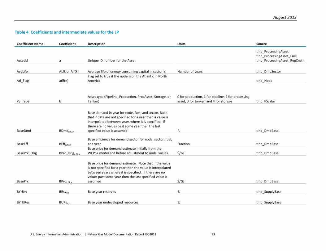
August 2013
U.S. Energy Information Administration | Natural Gas Model Documentation Report IEO2011 33
Table 4. Coefficients and intermediate values for the LP
Coefficient Name Coefficient Description Units Source
AssetId a Unique ID number for the Asset
tInp_ProcessingAsset, tInp_ProcessingAsset_Fuel, tInp_ProcessingAsset_RegCnstr
AvgLife ALfk or Alf(k) Average life of energy consuming capital in sector k Number of years tInp_DmdSector
Atl_Flag atlf(n) Flag set to true if the node is on the Atlantic in North America tInp_Node
PS_Type b Asset type (Pipeline, Production, ProcAsset, Storage, or Tanker)
0 for production, 1 for pipeline, 2 for processing asset, 3 for tanker, and 4 for storage tInp_PScalar
BaseDmd BDmdn,f,k,y
Base demand in year for node, fuel, and sector. Note that if data are not specified for a year then a value is interpolated between years where it is specified. If there are no values past some year then the last specified value is assumed PJ tInp_DmdBase
BaseEff BEffn,f,k,y Base efficiency for demand sector for node, sector, fuel, and year Fraction tInp_DmdBase
BasePrc_Orig BPrc_Orign,f,k,y Base price for demand estimate initially from the WEPS+ model and before adjustment to nodal values. $/GJ tInp_DmdBase
BasePrc BPrcn,f,k,y
Base price for demand estimate. Note that if the value is not specified for a year then the value is interpolated between years where it is specified. If there are no values past some year then the last specified value is assumed $/GJ tInp_DmdBase
BYrRsv BRsvn,c Base year reserves EJ tInp_SupplyBase
BYrURes BURsn,c Base year undeveloped resources EJ tInp_SupplyBase

August 2013
U.S. Energy Information Administration | Natural Gas Model Documentation Report IEO2011 34
Table 4. Coefficients and intermediate values for the LP (cont.)
Coefficient Name Coefficient Description Units Source
SupCatId c Unique Id for the supply category – Note set to “All” now
tInp_SupplyBase,
tInp_SupplyCat,
tInp_SupplyCatAsgn,
tInp_SupplyCatCnst
Capacity_Increment CapIa Capacity increments required for investment PJ/day of primary output fuel tInp_ProcessingAsset
Capacity_Increment CapIg Capacity increments required for investment EJ of working capacity tInp_StorageAsset
Capacity_Increment CapIp Capacity increment for capacity increases PJ/day tInp_PipelineAsset
Capacity_Increment CapIt
Capacity increment for capacity increases – adjusted for
expected utilization Pj per ship tInp_TankerAsset
CarContent CarCf CO2 content of the fuel Tonne CO2/GJ tInp_Fuel
Availability CCnstn,c,y
Share of reserves and undiscovered resources by node and
by supply category that is available to be developed in
specified year. Note that if data are not specified for a year
then a value is interpolated between years where it is
specified. If there are no values past some year then the
last specified value is assumed Fraction tInp_SupplyCatCnst

August 2013
U.S. Energy Information Administration | Natural Gas Model Documentation Report IEO2011 35
Table 4. Coefficients and intermediate values for the LP (cont.)
Coefficient Name Coefficient Description Units Source
Asset Construction Flag CFa,x,y Flag if capacity from asset type a, started in year x, is under construction in year y
1.0 if x+NYPa ≤ y <x+NYPa+NYCa
and 0.0 otherwise
Pipeline Construction Flag CFp,x,y
Flag if capacity from pipeline p, started in year x, is under construction in year y
1.0 if x+NYPp ≤ y <x+NYPp+NYCp
and 0.0 otherwise
Tanker Construction Flag CFt,x,y Flag if capacity from tanker t, started in year x, is under construction in year y
1.0 if
x+NYPt ≤ y <x+NYPt+NYCt and 0.0 otherwise
Storage Construction Flag CFg,x,y
Flag if capacity from storage g, started in year x, is under construction in year y
1.0 if x+NYPg ≤ y <x+NYPg+NYCg
and 0.0 otherwise
Number of years in year group CG(y), GCy
Number of years in the time group with marker year y, a time group is a group of years that are combined in the LP to reduce processing time
CTax_Scen CTax_Scenn,y Tax on CO2 used in the INGM scenario $2006/tonne CO2e tInp_CTax
CTax CTaxn,y Tax on CO2 assumed in the WEPS+ model and used to estimate the base demand $2006/tonne CO2e tInp_CTax
SeasAllocFac DmdSn,k,s Allocation factor for seasonal demand. Sum over seasons of SeasAllocFac*NDs/365 must equal 1.0 Fraction tInp_DmdSeasAlloc
Dst_NodeId dn(l) NodeId of the other end of the link tInp_PorttoPort
Dst_NodeId dn(p) NodeId of the node at the end of the pipeline tInp_PipelineAsset

August 2013
U.S. Energy Information Administration | Natural Gas Model Documentation Report IEO2011 36
Table 4. Coefficients and intermediate values for the LP (cont.)
Coefficient Name Coefficient Description Units Source
Fuel index for processed natural gas DNG Fuel index for processed natural gas
PriceElas DPEk or DPE(k) Price elasticity for demand in demand sector k Ratio tInp_DmdSector
DRate DRate Global discount rate Fraction (.12 is 12%) tInp_Scenario
DRate DRr Discount rate for the region fraction tInp_Region_Scn
Dry gas flag Dryf Set to 1 if f = DNG and 0 otherwist
Demand scaling factor DSFn,k,i,y Scaling factor for demand in region r for sector k in year y and for price step i Fraction
See section Calculation of DSF Values below
DistMar DstMarn,f,k,y Distribution Margin $/GJ tInp_DmdBase
MinCntrrFlag EI_Cnstr,y Flag if export/import constraint is annual and not seasonal True/False tInp_ImpExp_Cnstr
ExpCnstr ExpLmtr,f,y Annual limit on exports from the region and only used if FuelId is null EJ tInp_ImpExp_Cnstr
End_Year EYear Last year of optimization Year tInp_Scenario
LYear EYn,a,sy Last year that following data apply for (e.g., 2010) – inclusive Year tInp_ProcessingAsset_RegCnstr
LYear EYn,g,sy Last year that following data apply for (e.g., 2010) – inclusive Year tInp_StorageAsset_RegCnstr
LYear EYp,sy Last year that following data apply for (e.g., 2010) – inclusive Year tInp_PipelineAsset_Cnstr

August 2013
U.S. Energy Information Administration | Natural Gas Model Documentation Report IEO2011 37
Table 4. Coefficients and intermediate values for the LP (cont.)
Coefficient Name Coefficient Description Units Source
LYear EYt,sy Last year that following data apply for (e.g., 2010) – inclusive Year tInp_TankerAsset_Cnstr
FuelId f Unique ID for the fuel type
tInp_DmdBase, tInp_Fuel, tInp_Fuel_Scn, tInp_OthDmd, tInp_ProcessingAsset_Fuel
FuelId f(a) Id of primary output fuel (capacity is measure on output of this fuel) tInp_ProcessingAsset
FuelId f(g) Id of fuel type storded tInp_StorageAsset
FuelId f(p) ID of fuel type that the pipeline transports tInp_PipelineAsset
Fixed_OaM_Cost FOaMCa Annual fixed operating and maintenance cost per year $mil per year per capacity increment tInp_ProcessingAsset
Fixed_OaM_Cost FOaMCg Annual fixed operating and maintenance cost $mil per year tInp_StorageAsset
Fixed_OaM_Cost FOaMCp Annual fixed operating and maintenance cost per year $mil per year per capacity increment tInp_PipelineAsset
Fixed_OaM_Cost FOaMCt Annual fixed operating and maintenance cost $mil per year per ship tInp_TankerAsset
FuelId fp(r) Unique ID for the fuel type used to index the minimum price on tInp_ImpExp_Cnstr
Fuel use FUg Fuel use from the injection and withdrawal and including losses applied on injections Fraction as a percentage of injections tInp_StorageAsset
Fuel_Use FUp Pipeline fuel use fraction tInp_PipelineAsset

August 2013
U.S. Energy Information Administration | Natural Gas Model Documentation Report IEO2011 38
Table 4. Coefficients and intermediate values for the LP (cont.)
Coefficient Name Coefficient Description Units Source
StorageId g Unique ID number for the Asset tInp_StorageAsset, tInp_StorageAsset_RegCnstr
GovtTake Govtn The government share of the natural gas sales price Fraction tInp_Node_Scn
Investment_Cost ICsta Investment cost per year $mil per year per capacity increment tInp_ProcessingAsset
Investment_Cost ICstg Investment cost per year $mil per year tInp_StorageAsset
Investment_Cost ICstp Investment cost per year $mil per year per capacity increment tInp_PipelineAsset
Investment_Cost ICstt Investment cost per year $mil per year per ship tInp_TankerAsset
ImpCnstr ImpLmtr,f,y Annual limit on imports to the region and only used if FuelId is null EJ tInp_ImpExp_Cnstr
Inp_FuelId Inpf(t) Id of input fuel to tanker tInp_TankerFuel
InvCnstr InvCr,y Investment costraint for the region and only used if FuelId is null Million $ tInp_ImpExp_Cnstr
DmdSectorId k Unique Id for the demand sector
tInp_DmdBase, tInp_DmdSeasAlloc, tInp_DmdSector
PorttoPortId l Id of Port-to-port link tInp_PorttoPort
Loading Time LdTt The number of days required to load the ship Days tInp_TankerAsset
Last year in time horizon LY The last year in the time horizon Year
SMPrcStep m Major price step for supply category (0, 1, 2, …) tInp_SupplyBase, tInp_SupplyCatAsgn

August 2013
U.S. Energy Information Administration | Natural Gas Model Documentation Report IEO2011 39
Table 4. Coefficients and intermediate values for the LP (cont.)
Coefficient Name Coefficient Description Units Source
m(n,c,i) Major price step that the minor price step is part of tInp_SupplyBase
Min_Capacity MnCapn,a,sy Minimum capacity addition allowed in the node PJ/day output of primary fuel tInp_ProcessingAsset_RegCnstr
Min_Capacity MnCapn,g,sy Minimum capacity addition allowed in the node PJ working gas tInp_StorageAsset_RegCnstr
Min_Capacity MnCapp,sy Minimum capacity addition allowed for the pipeline PJ/day of input fuel to pipeline tInp_PipelineAsset_Cnstr
Min_Capacity MnCapt,sy Minimum capacity addition allowed for the tanker type Number of ships tInp_TankerAsset_Cnstr
MnCapAn,g,sy MnCapAn,g,sy Minimum capacity for storage adjusted for storage fraction PJ MnCapn,g,sy * StorFrac
MxCapAn,g,sy MxCapAn,g,sy Maximum capacity for storage adjusted for storage fraction PJ MxCapn,g,sy * StorFrac
MinFlow_Flag mnfflg(l)
Flag if minimum flow is to be assigned to the port-to-port link and is used to control prices for the NGTDM interface. The minimum flow 1e-7 PJ tanker capacity Yes/No tInp_PorttoPort
MnPrc MnPn,c,m Minimum development costs at which reserves come online $/GJ tInp_SupplyBase
MinPrc_Fac MnPrcFr
Factor for minimum price equation to be multiplied for price for specified fuel. Note that it is specified for only one year but applies to all Ratio tInp_ImpExp_Cnstr
MinPrc_Int MnPrcIr Intercept for minimum price equation. Note that it is specified for only one year but applies to all $/GJ tInp_ImpExp_Cnstr
Max_Capacity MxCapn,a,sy Maximum capacity addition allowed in the node PJ/day output of primary fuel tInp_ProcessingAsset_RegCnstr

August 2013
U.S. Energy Information Administration | Natural Gas Model Documentation Report IEO2011 40
Table 4. Coefficients and intermediate values for the LP (cont.)
Coefficient Name Coefficient Description Units Source
Max_Capacity MxCapn,g,sy Maximum capacity addition allowed in the node PJ working gas tInp_StorageAsset_RegCnstr
Max_Capacity MxCapp,sy Maximum capacity addition allowed for the pipeline PJ/day of input fuel to pipeline tInp_PipelineAsset_Cnstr
Max_Capacity MxCapt,sy Maximum capacity addition allowed for the tanker type Number of ships tInp_TankerAsset_Cnstr
Maximum_Life MxLa Maximum operating life of asset (e.g., 30 years) Number Years tInp_ProcessingAsset
Maximum_Life MxLg Maximum operating life of asset (e.g., 30 years) Number Years tInp_StorageAsset
Maximum_Life MxLp Maximum operating life of asset (e.g., 30 years) Number Years tInp_PipelineAsset
Maximum_Life MxLt Maximum operating life of asset (e.g., 30 years) Number Years tInp_TankerAsset
MxPrc MxPn,c,m Maximum development costs at which reserves come online $/GJ tInp_SupplyBase
NodeId n Unique id for node
tInp_CTax, tInp_DmdBase, tInp_DmdSeasAlloc, tInp_Node, tInp_Node_Scn, tInp_ProcessingAsset_RegCnstr, tInp_StorageAsset_RegCnstr, tInp_SupplyBase, tInp_SupplyCatAsgn, tInp_SupplyCatCnst, tInp_TankerPort
NA_Flag naf(n) Flag set to true if the node is in North America tInp_Node

August 2013
U.S. Energy Information Administration | Natural Gas Model Documentation Report IEO2011 41
Table 4. Coefficients and intermediate values for the LP (cont.)
Coefficient Name Coefficient Description Units Source
NA_Flag naf(r) Flag set to true if the region is in North America tInp_Region
NumDays NDs Number of days in the season Days tInp_Season_Scn
NFCstgs NFCstsn,f,k,y Non-fuel costs in using fuel $/GJ tInp_DmdBase
NGL Flag NGLf Set to 1 if the fuel f is NGLs
NGL_Frac NGLFn,c,m Fraction of wet gas that is NGLs Fraction tInp_SupplyBase
Num_MinPrcStp NPSn,c,m Number of minor price steps within major price step number tInp_SupplyBase
Num_Yrs_Inv NYCa Number of years required for construction Number Years tInp_ProcessingAsset
Num_Yrs_Inv NYCg Number of years required for construction Number Years tInp_StorageAsset
Num_Yrs_Inv NYCp Number of years required for construction Number Years tInp_PipelineAsset
Num_Yrs_Inv NYCt Number of years required for construction Number Years tInp_TankerAsset
Num_Yrs_PlnAppr NYPa Number of years required for planning and approvals Number Years tInp_ProcessingAsset
Num_Yrs_PlnAppr NYPg Number of years required for planning and approvals Number Years tInp_StorageAsset
Num_Yrs_PlnAppr NYPp Number of years required for planning and approvals Number Years tInp_PipelineAsset
Num_Yrs_PlnAppr NYPt Number of years required for planning and approvals Number Years tInp_TankerAsset
Asset Operational Flag OFa,x,y Flag if capacity from asset type a, started in year x, is operational in year y
1.0 if
x+NYPa+NYCa ≤ y <x+NYPa+NYCa+MxLa
and 0.0 otherwise

August 2013
U.S. Energy Information Administration | Natural Gas Model Documentation Report IEO2011 42
Table 4. Coefficients and intermediate values for the LP (cont.)
Coefficient Name Coefficient Description Units Source
Pipeline Operation Flag OFp,x,y Flag if capacity from pipeline p, started in year x, is operational in year y
1.0 if
x+NYPp+NYCp ≤ y <x+NYPp+NYCp+MxLp and 0.0 otherwise
Tanker Operational Flag OFt,x,y Flag if capacity from tanker t, started in year x, is operational in year y
1.0 if
x+NYPt+NYCt ≤ y <x+NYPt+NYCt+MxLt
and 0.0 otherwise\
Storage Operational Flag OFg,x,y Flag if capacity from storage g, started in year x, is operational in year y
1.0 if
x+NYPg+NYCg ≤ y <x+NYPg+NYCg+MxLg and 0.0 otherwise\
Org_NodeId on(l) NodeId of one end of the link tInp_PorttoPort
Org_NodeId on(p) NodeId of the node at the start of the pipeline tInp_PipelineAsset
ODPrc OPrcf,y Price of fuel in the market (applies only to NGLs, GTLs, and reinjected gas) $/GJ tInp_OthDmd
OthFU OthFUn
Fraction of secondary demand used for internal pipelines and distribution and not captured in the specified pipelines Fraction tInp_Node_Scn
Out_FuelId Outf(t) Id of output fuel to tanker corresponding to input fuel tInp_TankerFuel

August 2013
U.S. Energy Information Administration | Natural Gas Model Documentation Report IEO2011 43
Table 4. Coefficients and intermediate values for the LP (cont.)
Coefficient Name Coefficient Description Units Source
PipelineId p Unique ID for the pipeline tInp_PipelineAsset, tInp_PipelineAsset_Cnstr
PlanAppr_Cst PACsta Annual Planning and Approval costs $mil per year per capacity increment tInp_ProcessingAsset
PlanAppr_Cst PACstg Annual Planning and Approval costs $mil per year tInp_StorageAsset
PlanAppr_Cst PACstp Annual Planning and Approval costs $mil per year per capacity increment tInp_PipelineAsset
PlanAppr_Cst PACstt Annual Planning and Approval costs $mil per year per ship tInp_TankerAsset
ProdIEffBase PEffBn Base Value for production inefficiency for node – reduces the share of economic resources that can be developed Fraction tInp_Node_Scn
ProdIEffImp PEffIn Annual improvement in production inefficiency value with total share capped at 1.0 Fraction/Year tInp_Node_Scn
Asset Planning Flag PFa,x,y Flag if capacity from asset type a, started in year x, is in planning in year y
1.0 if x ≤ y <x+NYPa and 0.0 otherwise
Pipeline Planning Flag PFp,x,y Flag if capacity from pipeline p, started in year x, is in planning in year y
1.0 if x ≤ y <x+NYPp and 0.0 otherwise
Tanker Planning Flag PFt,x,y Flag if capacity from tanker t, started in year x, is in planning in year y
1.0 if x ≤ y <x+NYPt
and 0.0 otherwise
Storage Planning Flag PFg,x,y Flag if capacity from storage g, started in year x, is in planning in year y
1.0 if x ≤ y <x+NYPg
and 0.0 otherwise

August 2013
U.S. Energy Information Administration | Natural Gas Model Documentation Report IEO2011 44
Table 4. Coefficients and intermediate values for the LP (cont.)
Coefficient Name Coefficient Description Units Source
Production factor for
previous years reserves PFac1n,c,m,y
Used to apply against the beginning of year reserves for the year group. This equation sums up the PR ratios times the remaining reserves within the year group and averages Ratio
(1- PRBn,c,m,y CG(y))/CGy *
1000/365 = ∑y’,
g(y’)=yPRBn,c,m,y*(1-PRBn,c,m,y)(y’-
y)/CGy*1000/365
Production factor
reserve adds PFac2n,c,m,y
Used to apply against the total reserve additions for the year group. It simulates an equal fraction of the reserves added in each year and reserve depletion over the remaining years in the year group. Ratio
1000/365 * (CGy - (1-
PRBn,c,m,yCG(y))/ (1-
PRBn,c,m,y)*PRBn,c,m,y)/CGy2
Factor for adjusting supply costs PFac3n,c,m,y
This factor adjusts the costs of the reserve additions to account for only production within the time horizon. It equals the sum of production that starts in each year of the time group that contains the marker year y. Ratio
∑x=SYG(y) to LY{(PrAn,c,m/CGy) * (1- PRBn,c,m(x-SYG(y)))/ (1- PRBn,c,m)}
Adjusted P/R ratio PREn,c,m P/R ratio for node and supply category but adjusted to work against end or year reserves Ratio PRn,c,m / (1- PRn,c,m)
Production Factor Beta PRBn,c,m 1 minus P/R ratio for node and supply category but adjusted to work against end of year reserves Ratio
(1-PREn,c,m)
Port_Capacity PortCn The maximum number of ships in the port at any one time for loading or unloading – not currently used Number ships per day tInp_Node_Scn
PrcSub PrcSubn,f,k,y
Price subsidy assumed for the input demand assumptions for the wholesale price on average for the region. $/GJ tInp_DmdBase

August 2013
U.S. Energy Information Administration | Natural Gas Model Documentation Report IEO2011 45
Table 4. Coefficients and intermediate values for the LP (cont.)
Coefficient Name Coefficient Description Units Source
PrcSub_Scn PrcSubSn,f,k,y
Price subsidy used to estimate demand for demand assumptions for the wholesale price on average for the region. $/GJ tInp_DmdBase
PR_Ratio PRn,c,m Maximum production to reserves ratio ratio tInp_SupplyBase
PScalar PScalarb,y Cost scalar reflecting both increases in asset/production costs and technological improvement Ratio tInp_PScalar
Qty Qtya,f Quantity input (negative) or output (positive) for capacity increment PJ/day tInp_ProcessingAsset_Fuel
RegionId r RegionId of region that the constraint applies to tInp_ImpExp_Cnstr, tInp_Region, tInp_Region_Scn
RegionId r(n) RegionId of region in which node n is located tInp_Node_Scn
CmbImpExp_RegionId rc(r) Id of Region used as aggregate region for combined import/export constraint tInp_Region_Scn
Retirement_Cost RCsta Cost of retiring the asset $mil per year per capacity increment tInp_ProcessingAsset
Retirement_Cost RCstg Cost of retiring the asset $mil tInp_StorageAsset
Retirement_Cost RCstp Cost of retiring the asset $mil per year per capacity increment tInp_PipelineAsset
Retirement_Cost RCstt Cost of retiring the asset $mil per year per capacity increment tInp_TankerAsset
Asset Decommission Flag RFa,x,y Flag if capacity from asset type a, started in year x, is being decomissioned in year y
1.0 if y = x+NYPa+NYCa+MxLa
and 0.0 otherwise

August 2013
U.S. Energy Information Administration | Natural Gas Model Documentation Report IEO2011 46
Table 4. Coefficients and intermediate values for the LP (cont.)
Coefficient Name Coefficient Description Units Source
Pipeline Decommission Flag RFp,x,y
Flag if capacity from pipeline p, started in year x, is being decomissioned in year y
1.0 if y = x+NYPp+NYCp+MxLp
and 0.0 otherwise
Tanker Decommission Flag RFt,x,y
Flag if capacity from tanker t, started in year x, is being decomissioned in year y
1.0 if y = x+NYPt+NYCt+MxLt
and 0.0 otherwise
Storage Decommission Flag RFg,x,y
Flag if capacity from storage g, started in year x, is being decomissioned in year y
1.0 if y = x+NYPg+NYCg+MxLg
and 0.0 otherwise
Regas_Cap RGFt Flag is True if tanker has regasification capability built onboard True/False tInp_TankerAsset
Reinjected gas point RIG Index to fuel which is reinjected gas to get value of the gas for other purposes
Resource qty at cumulative price step RRQn,c,j
Remaining reserves at price step j (including lower prices) EJ
BURsn,c,m * [(SPrcn,c,j – MnPn,c,m)/ [(MxPn,c,m – MnPn,c,m)] α(n,c,m) RRQn,c,0 is set to the value 0 where 1 is the first step
RsvShr RsvSn,c,m Share of economic/undeveloped resources that can be developed in the year Fraction tInp_SupplyBase
SeasonId s Unique id for season tInp_DmdSeasAlloc, tInp_Season, tInp_Season_Scn

August 2013
U.S. Energy Information Administration | Natural Gas Model Documentation Report IEO2011 47
Table 4. Coefficients and intermediate values for the LP (cont.)
Coefficient Name Coefficient Description Units Source
SeasonId s Unique ID number for the season tInp_Season, tInp_Season_Scn
SeasonId s Unique ID number for the season tInp_Season_Scn
Scale_Flag ScaleFlag Flag set to true if demand is to be based on another baseline demand option scaled and false otherwise tInp_AA_Dmd_Spec
Sn,c,j
The incremental order of the minor price step within the major price step. For example if 16 is the first minor price step for major price step 4 and 20 is the last minor price step for price step 4 then s(n,c,16) is 1 and s(n,c,20) is 5. tInp_SupplyBase
Non-variable costs of supply in minor price step SPrcn,c,j,y
Non-variable costs of supply in minor price step set equal to point between minimum and maximum supply price for the major price step $/GJ
MnPn,c,m(n,c,j) + (MxPn,c,m(n,c,j) - MnPn,c,m(n,c,j))/ NPSn,c,m(n,c,j)
ScnPrc SPrcn,f,k,y Scenario price for scenario estimation $/GJ tInp_DmdBase
Adjusted price for resource additions reflecting regional price constraints SPrcAn,c,j,y
Adjusted price for supply step reflecting regional price constraints. Some differentiation allowed for prices below minimum regional price. $/GJ
Max{SPrcBn,c,j, SPrcn,c,j0.05 *
(MnPrcIr + MnPrcFr * OPrcf
fp(r),y}0.95}
Adjusted price for resource additions reflecting production through end of the time period SPrcBn,c,j,y
Adjusted price for resource additions reflecting production through end of the time period and regional price constraints. $/GJ
Min{SPrcn,c,j,y*Pscalar0,y/(1-Govtn), SPrcn,c,j,y*Pscalar0, + Govtn * 4.0) * PFac3n,c,m,y*1000
Storage_Fraction StorFrac Fraction of storage working gas that can be effectively used Fraction Tlnp_Scenario
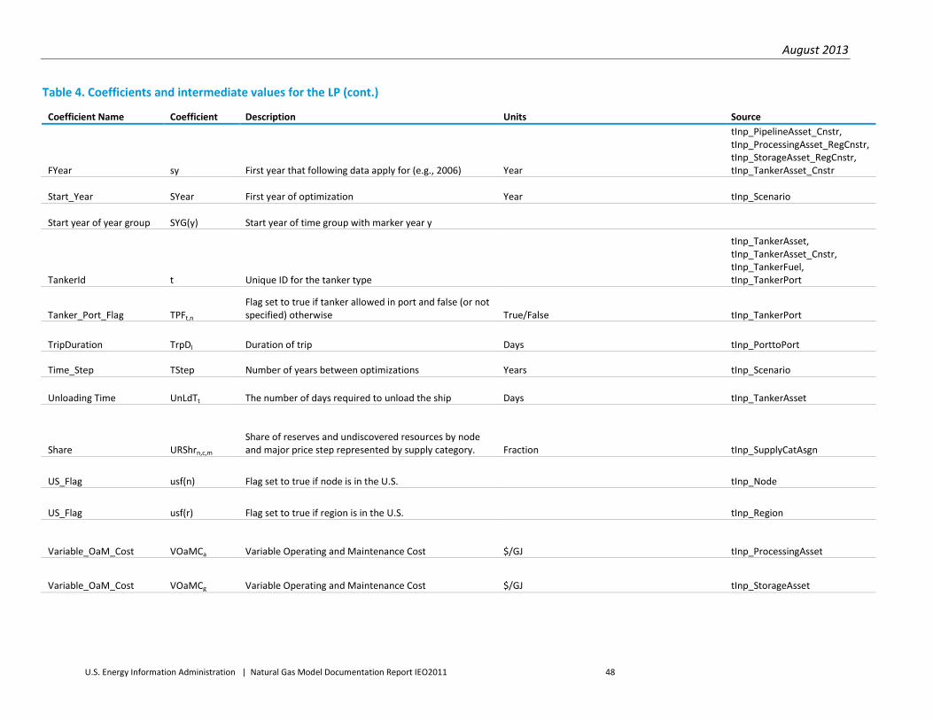
August 2013
U.S. Energy Information Administration | Natural Gas Model Documentation Report IEO2011 48
Table 4. Coefficients and intermediate values for the LP (cont.)
Coefficient Name Coefficient Description Units Source
FYear sy First year that following data apply for (e.g., 2006) Year
tInp_PipelineAsset_Cnstr, tInp_ProcessingAsset_RegCnstr, tInp_StorageAsset_RegCnstr, tInp_TankerAsset_Cnstr
Start_Year SYear First year of optimization Year tInp_Scenario
Start year of year group SYG(y) Start year of time group with marker year y
TankerId t Unique ID for the tanker type
tInp_TankerAsset, tInp_TankerAsset_Cnstr, tInp_TankerFuel, tInp_TankerPort
Tanker_Port_Flag TPFt,n Flag set to true if tanker allowed in port and false (or not specified) otherwise True/False tInp_TankerPort
TripDuration TrpDl Duration of trip Days tInp_PorttoPort
Time_Step TStep Number of years between optimizations Years tInp_Scenario
Unloading Time UnLdTt The number of days required to unload the ship Days tInp_TankerAsset
Share URShrn,c,m Share of reserves and undiscovered resources by node and major price step represented by supply category. Fraction tInp_SupplyCatAsgn
US_Flag usf(n) Flag set to true if node is in the U.S. tInp_Node
US_Flag usf(r) Flag set to true if region is in the U.S. tInp_Region
Variable_OaM_Cost VOaMCa Variable Operating and Maintenance Cost $/GJ tInp_ProcessingAsset
Variable_OaM_Cost VOaMCg Variable Operating and Maintenance Cost $/GJ tInp_StorageAsset
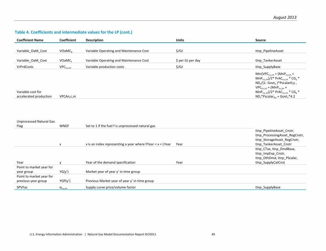
August 2013
U.S. Energy Information Administration | Natural Gas Model Documentation Report IEO2011 49
Table 4. Coefficients and intermediate values for the LP (cont.)
Coefficient Name Coefficient Description Units Source
Variable_OaM_Cost VOaMCp Variable Operating and Maintenance Cost $/GJ tInp_PipelineAsset
Variable_OaM_Cost VOaMCt Variable Operating and Maintenance Cost $ per GJ per day tInp_TankerAsset
VrPrdCosts VPCn,c,m Variable production costs $/GJ tInp_SupplyBase
Variable cost for accelerated production VPCAn,c,m
Min{VPCn,c,m + (MnPn,c,m + MnPn,c,m)/2* PrACn,c,m * CGy * NDs/(1- Govtn )*Pscalar0,y , VPCn,c,m + (MnPn,c,m + MnPn,c,m)/2* PrACn,c,m * CGy * NDs*Pscalar0,y + Govtn*4.2
Unprocessed Natural Gas Flag WNGf Set to 1 if the fuel f is unprocessed natural gas
x x is an index representing a year where FYear < x < LYear Year
tInp_PipelineAsset_Cnstr, tInp_ProcessingAsset_RegCnstr, tInp_StorageAsset_RegCnstr, tInp_TankerAsset_Cnstr
Year y Year of the demand specification Year
tInp_CTax, tInp_DmdBase, tInp_ImpExp_Cnstr, tInp_OthDmd, tInp_PScalar, tInp_SupplyCatCnst
Point to market year for year group YG(y’) Market year of year y’ in time group Point to market year for previous year group YGP(y’) Previous Market year of year y’ in time group
SPVFac αn,c,m Supply curve price/volume factor tInp_SupplyBase
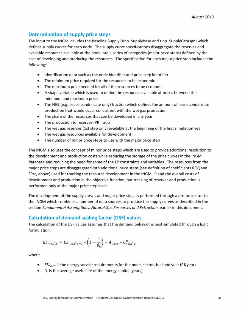
August 2013
U.S. Energy Information Administration | Natural Gas Model Documentation Report IEO2011 50
Determination of supply price steps The input to the INGM includes the Baseline Supply (tInp_SupplyBase and tInp_SupplyCatAsgn) which defines supply curves for each node. The supply curve specifications disaggregate the reserves and available resources available at the node into a series of categories (major price steps) defined by the cost of developing and producing the resources. The specification for each major price step includes the following:
• Identification data such as the node identifier and price step identifier • The minimum price required for the resources to be economic • The maximum price needed for all of the resources to be economic • A shape variable which is used to define the resources available at prices between the
minimum and maximum price • The NGL (e.g., lease condensate only) fraction which defines the amount of lease condensate
production that would occur concurrent with the wet gas production • The share of the resources that can be developed in any year • The production to reserves (PR) ratio • The wet gas reserves (1st step only) available at the beginning of the first simulation year • The wet gas resources available for development • The number of minor price steps to use with the major price step
The INGM also uses the concept of minor price steps which are used to provide additional resolution to the development and production costs while reducing the storage of the price curves in the INGM database and reducing the need for some of the LP constraints and variables. The resources from the major price steps are disaggregated into additional price steps (see definition of coefficients RRQ and SPrc, above) used for tracking the resource development in the INGM LP and the overall costs of development and production in the objective function, but tracking of reserves and production is performed only at the major price step level.
The development of the supply curves and major price steps is performed through a pre-processor to the INGM which combines a number of data sources to produce the supply curves as described in the section Fundamental Assumptions, Natural Gas Resources and Extraction, earlier in this document.
Calculation of demand scaling factor (DSF) values The calculation of the DSF values assumes that the demand behavior is best simulated through a logit formulation:
𝐸𝑆𝑛,𝑘,𝑓,𝑦 = 𝐸𝑆𝑛,𝑘,𝑓,𝑦−1 ∗ �1 −1𝛽𝑘� + 𝐴𝑛,𝑘,𝑦 ∗ 𝐶𝑛,𝑘,𝑓,𝑦
𝛼
where
• ESn,k,f,y is the energy service requirements for the node, sector, fuel and year (PJ/year) • βk is the average useful life of the energy capital (years)

August 2013
U.S. Energy Information Administration | Natural Gas Model Documentation Report IEO2011 51
• An,k,y is a regional intercept for the node, sector and year (PJ/Year/$/GJ) • Cn,k,f,y is the cost of providing the energy service for the node, sector, fuel, and year ($/GJ) • α is the price elasticity (fraction)
𝐷𝑚𝑑𝑛,𝑘,𝑓,𝑦 = 𝐸𝑆𝑛,𝑘,𝑓,𝑦/𝐸𝑓𝑓𝑛,𝑘,𝑓,𝑦
where
• Dmdn,k,f,y is the energy demand for the node, sector, fuel and year (PJ/year) • Effn,k,f,y is the relative energy efficiency of the demand sector for the node, sector, fuel, and year
(fraction)
𝐶𝑛,𝑘,𝑓,𝑦 =𝑃𝑛,𝑘,𝑓,𝑦 + 𝑃𝑟𝑐𝑆𝑢𝑏𝑛,𝑘,𝑓,𝑦 + 𝐶𝑇𝑎𝑥𝑛,𝑦 ∗ 𝐶𝑎𝑟𝐶𝑓 + 𝐷𝑖𝑠𝑡𝑀𝑎𝑟𝑛,𝑘,𝑓,𝑦
𝐸𝑓𝑓𝑛,𝑘,𝑓,𝑦+ 𝑁𝐹𝐶𝑠𝑡𝑠𝑛,𝑘,𝑓,𝑦
+ 𝐴𝑑𝑓𝐹𝑛,𝑘,𝑓,𝑦
where
• Pn,f,y is the energy price for the node, fuel, and year ($/GJ) and the input value Prcn,f,k,y is used in the initial estimation of the AdjFn,k,f,y but the value SPrcn,f,k,y is used in the actual modeling
• PrcSubn,k,f,y is the price subsidy applied in the node for the sector, fuel, and year ($/GJ) • CTaxn,y is the CO2 tax for the node and year ($/tonne CO2) • CarCf is the CO2 content of the fuel (tonne CO2/GJ) • DistMarn,k,f,y is the distribution margin for the node, sector,fuel and year ($/GJ) • NFCstsn,k,f,y are the non-fuel costs of converting the fuel to energy service ($/GJ) • AdjFn,k,f,y is an availability adjustment factor for the node, sector, fuel, and year which also
includes non-fuel costs ($/GJ)
𝐸𝑆𝐼𝑛,𝑘,𝑓,𝑦 = 𝐴𝑛,𝑘,𝑦 ∗ 𝐶𝑛,𝑘,𝑓,𝑦𝛼
where
• ESIn,k,f,y is the annual incremental energy service requirements for the node, sector, fuel and year (PJ/year)
𝑆ℎ𝑟𝑛,𝑘,𝑓,𝑦 =𝐴𝑛,𝑘,𝑦 ∗ 𝐶𝑛,𝑘,𝑓,𝑦
𝛼
=𝐶𝑛,𝑘,𝑓,𝑦𝛼
∑ 𝐶𝑛,𝑘,𝑓,𝑦𝛼
𝑓
where Shrn,k,f,y is the share of the incremental energy service requirement for node, sector and year satisfied with the fuel f (fraction)
The first step is to adjust the price subsidy so that the resulting price is no less than $0.75/GJ. We then estimate the annual incremental energy service requirement as follows:
• When y is the start year:
𝐸𝑆𝐼𝑛,𝑘,𝑓,𝑦 = 𝐷𝑚𝑑𝑛,𝑘,𝑓,𝑦 ∗ 𝐸𝑓𝑓𝑛,𝑘,𝑓,𝑦

August 2013
U.S. Energy Information Administration | Natural Gas Model Documentation Report IEO2011 52
Otherwise
𝐸𝑆𝐼𝑛,𝑘,𝑓,𝑦 = 𝐷𝑚𝑑𝑛,𝑘,𝑓,𝑦 ∗ 𝐸𝑓𝑓𝑛,𝑘,𝑓,𝑦 − 𝐷𝑚𝑑𝑛,𝑘,𝑓,𝑦−1 ∗ 𝐸𝑓𝑓𝑛,𝑘,𝑓,𝑦−1 ∗ (1 − 1/𝛽𝑘)
We calculate the efficiency of the incremental energy service as follows:
• When y is the start year:
𝐸𝐹𝐹𝐼𝑛,𝑘,𝑓,𝑦 = 𝐸𝑆𝐼𝑛,𝑘,𝑓,𝑦/(𝐷𝑚𝑑𝑛,𝑘,𝑓,𝑦)
• Otherwise
𝐸𝐹𝐹𝐼𝑛,𝑘,𝑓,𝑦 = 𝐸𝑆𝐼𝑛,𝑘,𝑓,𝑦/(𝐷𝑚𝑑𝑛,𝑘,𝑓,𝑦 − 𝐷𝑚𝑑𝑛,𝑘,𝑓,𝑦−1 ∗ (1 − 1𝛽𝑘
))
We then calculate the estimated share for each fuel type as:
𝑆ℎ𝑟𝑛,𝑘,𝑓,𝑦 =𝐸𝑆𝐼𝑛,𝑘,𝑓,𝑦
∑ 𝐸𝑆𝐼𝑛,𝑘,𝑓′,𝑦𝑓′
The next step is to calculate the values of C and AdjFn,k,f,y where
𝐶 =
and for all f
𝐴𝑑𝑗𝐹𝑛,𝑘,𝑓,𝑦 = max {0, (𝑆ℎ𝑟𝑛,𝑘,𝑓,𝑦 ∗ 𝐶)�1𝑎� −
𝑃𝑛,𝑓,𝑦
𝐸𝑓𝑓𝑛,𝑘,𝑓,𝑦}
The value of An,k,y is then calculated for the fuel, f, natural gas as:
𝐴𝑛,𝑘,𝑦 = 𝐸𝑆𝐼𝑛,𝑘,𝑓,𝑦/𝐶𝑛,𝑘,𝑓,𝑦𝛼
where :
𝐶𝑛,𝑘,𝑓,𝑦 =𝑃𝑛,𝑓,𝑦 + 𝑃𝑟𝑐𝑆𝑢𝑏𝑛,𝑘,𝑓,𝑦 + 𝐶𝑇𝑎𝑥𝑛,𝑦 ∗ 𝐶𝑎𝑟𝐶𝑓 + 𝐷𝑖𝑠𝑡𝑀𝑎𝑟𝑛,𝑘,𝑓,𝑦
𝐸𝑓𝑓𝑛,𝑘,𝑓,𝑦+ 𝑁𝐹𝐶𝑠𝑡𝑠𝑛,𝑘,𝑓,𝑦 + 𝐴𝑑𝑓𝐹𝑛,𝑘,𝑓,𝑦
The natural gas demand can then be estimated for different natural gas prices by applying these equations:
𝑇𝑆𝐹𝑛,𝑘,𝑖,𝑦 = (𝐴𝑛,𝑘,𝑓,𝑦 ∗ (𝐷𝑃𝑟𝑐𝑛,𝑘,𝑖,𝑦 + 𝑃𝑟𝑐𝑆𝑢𝑏𝑆𝑛,𝑘,𝑓,𝑦 + 𝐶𝑇𝑎𝑥𝑆𝑐𝑒𝑛𝑛,𝑦 ∗ 𝐶𝑎𝑟𝐶𝑓 + 𝐷𝑖𝑠𝑡𝑀𝑎𝑟𝑛,𝑘,𝑓,𝑦
𝐷𝐸𝑓𝑓𝑛,𝑘,𝑓,𝑦+ 𝑁𝐹𝐶𝑠𝑡𝑠𝑛,𝑘,𝑓,𝑦 + 𝐴𝑑𝑗𝐹𝑛,𝑘,𝑓,𝑦)
and
𝐷𝑆𝐹𝑛,𝑘,𝑖,𝑦 = 𝑇𝑆𝐹𝑛,𝑘,𝑖,𝑦 − 𝑇𝑆𝐹𝑛,𝑘,𝑖−1,𝑦
August 2013
U.S. Energy Information Administration | Natural Gas Model Documentation Report IEO2011 53
Where
• DPrcn,k,i,y is the modeled price for natural gas for the node n, sector k, step i, and year y • PrcSubSn,k,f,y is the subsidy used to estimate demand for demand assumptions for the wholesale
price on average for the region ($/GJ). • CTax_Scenn,y is the CO2 tax used for the INGM run for the node and year ($/tonne CO2)
Scaling The INGM allows for the base demand to be scaled. When this option is used (ScaleFlag = True) then the base demand for select regions are scaled based on the input scaling factors provided for the scenario.
Columns/activities The following table, Table 5, defines the columns in the LP and provides units, lower bounds and upper bounds.

August 2013
U.S. Energy Information Administration | Natural Gas Model Documentation Report IEO2011 54
Table 5. Columns in the LP
Column Name Description Lower Bound Upper Bound Units
DRsn,c,j,y Quantity of resources converted to reserves in node n for supply category c and minor price step j in year y 0
Min{ 1.0,∑y’,g(y’)=y RsvSn,c,m(n,c,j)) * EJ
Expr,y,s Exports from region r for fuel f in year y and season s 0
If EI_Cnstr,y then None,
otherwiseExpLmtr,f,y/365*1000 PJ/day
Impr,y,s Imports to region r for fuel f in year y and season s 0
If EI_Cnstr,y then None,
otherwiseImpLmtr,f,y/365*1000 PJ/day
NCIr,y,d Net costs from asset investments and operations for region r and year y when d is 1 and takes the value 0 when d is 0 0 None $mil
NCOr,y,d
Net costs minus revenues from all but asset investments for region r and year y – if costs are greater than revenues then NCOr,y,1 is positive and is the net costs and NCOr,y,0 takes the value 0 otherwise NCOr,y,1 takes the value 0 and NCOr,y,0 takes the net revenues minus costs 0 None $mil
ODn,f,y,s Other demand at node n for fuel f in year y and season s 0 None PJ/day
PLCpEp,x Pipeline capacity investment started for pipeline p in year x. 0 None PJ/day
PlCpUp,y,s
Pipeline capacity utilization for pipeline p, for year y, and for season s. Only where capacity data for p,x exists where x + NYPp,x + NYCp,x ≤ y < x + NYPp,x + NYCp,x + MxLp,x 0 None PJ/day
PrCpEn,a,x Processing capacity investment started for asset a, at node n, in year x. 0 None
PJ/Day measured as output of primary
output fuel
PrCpUn,a,y,s
Processing capacity utilization for asset a, at node n, for year y, and for season s. Only where regional capacity data for n,a,x exists where x + NYPn,a,x + NYCn,a,x ≤ y < x + NYPn,a,x + NYCn,a,x + MxLn,a,x 0 None PJ/day
PrAn,c,m,y,s Accelerated production for supply category c in node n, for major price step m, in year y and season s 0 None PJ/Day
Prdn,c,m,y,s Production for supply category c in node n, for major price step m, in year y and season s 0 None PJ/Day
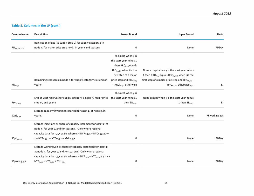
August 2013
U.S. Energy Information Administration | Natural Gas Model Documentation Report IEO2011 55
Table 5. Columns in the LP (cont.)
Column Name Description Lower Bound Upper Bound Units
RIJn,c,m=0,y,s
Reinjection of gas (to supply step 0) for supply category c in
node n, for major price step m=0, in year y and season s 0 None PJ/Day
RRn,c,j,y
Remaining resources in node n for supply category c at end of
year y
0 except when y is
the start year minus 1
then RRQn,c,i equals
RRQn,c,j-1 when i is the
first step of a major
price step and RRQn,c,j
– RRQn,c,j-1 otherwise
None except when y is the start year minus
1 then RRQn,c,j equals RRQn,c,j-1 when i is the
first step of a major price step and RRQn,c,j –
RRQn,c,j-1 otherwise,c,j-1 EJ
Rsvn,c,m,y
End-of-year reserves for supply category c, node n, major price
step m, and year y
0 except when y is
the start year minus 1
then BRsvn,c
None except when y is the start year minus
1 then BRsvn,c EJ
SCpEn,g,x
Storage capacity investment started for asset g, at node n, in
year x. 0 None PJ working gas
SCpIn,g,y,s
Storage injections as share of capacity increment for asset g, at
node n, for year y, and for season s. Only where regional
capacity data for n,g,x exists where x + NYPn,g,x + NYCn,g,x ≤ y <
x + NYPn,g,x + NYCn,g,x + MxLn,g,x 0 None PJ/Day
SCpWn,g,y,s
Storage withdrawals as share of capacity increment for asset g,
at node n, for year y, and for season s. Only where regional
capacity data for n,g,x exists where x + NYPn,g,x + NYCn,g,x ≤ y < x +
NYPn,g,x + NYCn,g,x + MxLn,g,x 0 None PJ/Day

August 2013
U.S. Energy Information Administration | Natural Gas Model Documentation Report IEO2011 56
Table 5. Columns in the LP (cont.)
Column Name Description Lower Bound Upper Bound Units
TCpEr,t,x Tanker capacity investment started for tanker t in year x for region r. 0 None PJ tanker capacity
TCpUt,fi,l,y,s
Tanker utilization for tanker t, using input fuel fi, for port-to-port link l, for year y, and for season s. Only where regional capacity data for t,x exists where x + NYPt,x + NYCt,x ≤ y < x + NYPt,x + NYCt,x + MxLt,x. Also, no t,l combinations allowed if TPFlt,on(l) or TPFLt,dn(l) are false.
0. if mnfflg(l) is false and 1e-7
otherwise None PJ tanker capacity
TDn,k,y Average daily demand for natural gas in node n for sector k in year y
0 if y > Syear and BDmdn,f=DNG,k,y
otherwise None if Y > Syear and BDmdn,f=DNG,k,y
otherwise PJ/day
TDSn,k,i,y Average daily demand for natural gas in node n for sector k in year y for price step i 0
∑YGP(y)<y’<y(DSFn,k,i,y’ * (1-1/Alfk)(y-y’) PJ/day

August 2013
U.S. Energy Information Administration | Natural Gas Model Documentation Report IEO2011 57
Constraints The following sections define the constraints in the LP. Each description includes the set of indices that the constraint applies to (e.g., all nodes), the units of the constraint, the name of the constraint, the sense of the constraint (e.g., less than or equal to), the right hand side of the constraint, and the coefficients for each column.
Objective (Obj) • Units: $mil discounted • Name: obj
� �−𝑁𝐶𝐼𝑟,𝑦,0 + 𝑁𝐶𝐼𝑟,𝑦,1 − 𝑁𝐶𝑂𝑟,𝑦,0 + 𝑁𝐶𝑂𝑟,𝑦,1�𝒓,𝒚
∗� 𝐷𝑅𝑎𝑡𝑒(𝑦′−𝑆𝑌𝑒𝑎𝑟)/𝐶𝐺𝑦𝑦𝑔(𝑦′)=𝑦
The net cash flows are accounted separately for operations and investments as NCOr,y,d and NCIr,y,d, respectively, so their sum represents producer net cash flows. The variables used to store these quantities are constrained to be non-negative, so a subscript d is introduced to denote the sign where d=0 is the positive value and d=1 is the negative value and 𝑁𝐶𝐼𝑟,𝑦,0 − 𝑁𝐶𝐼𝑟,𝑦,1 represents the net investment for the region and year while and 𝑁𝐶𝑂𝑟,𝑦,0 − 𝑁𝐶𝑂𝑟,𝑦,1 represents the net operating and maintenance costs for the region and year. The second sum represents the discount factor for year y. Finally, we desire to minimize the Objective Function, so we construct the negative of the discounted net cash flows.
Energy Balance Constraint (MB) This constraint forces the energy output to equal energy input for each node, fuel, year, and season.
• for all n, f, y, and s • Units: PJ/day • Constraint: MBn,f,y,s
In order, the equation includes the following:
• Input to the node (if Qtyaf is positive) or output to the node (otherwise) from gas processing by taking the utilization of the gas processing times the ratio of the input/output flow specifcation (Qtyaf) divided by the capacity assumed in the flow specification (CapIp) which is the unit flow of the fuel per PJ/day of utilization
• Input to node from the pipeline transport of the fuel to the node less fuel use during transport • Output from the node from pipeline transport • Input to the node from LNG transport minus fuel use during transport which is set to the tanker
utilization divided by the number of days required for the round trip including loading and unloading time, all times one mines the fuel use fraction
• Output from the node from LNG transport which is set to the tanker utilization divided by the number of days required for the round trip including loading and unloading time
• Output to demand which is the average hourly demand allocated to the season and scaled up to reflect pipeline fuel use not captured by the node to node pipelines

August 2013
U.S. Energy Information Administration | Natural Gas Model Documentation Report IEO2011 58
• Input from the production of wet gas from the field (times WNGf which is zero for all fuels except for wet gas)
• Input from the accelerated production of wet gas from the field (times WNGf which is zero for all fuels except for wet gas)
• Input of NGLs from the production of wet gas which equals the wet gas production times the ration of NGL production to wet gas production (NGLFn,c,m) times the flag NGLf which is set to one for NGLs and zero for all other fuels
• Input of NGLs from the accelerated production of wet gas which equals the wet gas production times the ration of NGL production to wet gas production (NGLFn,c,m) times the flag NGLf which is set to one for NGLs and zero for all other fuels
• Output representing other demand for the fuel at the node (note applicable for wet gas, dry gas, or LNG)
• Output representing storage injections at the node in the year and season • Input representing storage withdrawals at the node in the year and season • Output representings the reinjection of dry gas at the node for the year and season
� 𝑃𝑟𝐶𝑝𝑈𝑛,𝑎,𝑦,𝑠𝒂
∗𝑄𝑡𝑦𝑎𝑓𝐶𝑎𝑝𝐼𝑝
+ � 𝑃𝐼𝐶𝑝𝑈𝑝,𝑦,𝑠,𝑑𝑛(𝑝)=𝑛,𝑓(𝑝)=𝑓 ∗ (1 − 𝐹𝑈𝑝)𝑎
−� 𝑃𝐼𝐶𝑝𝑈𝑝,𝑦,𝑠,𝑜𝑛(𝑝)=𝑛,𝑓(𝑝)=𝑓 +𝑎
� 𝑇𝐶𝑝𝑈𝑡,𝑓𝑖,;,𝑠,𝑦,𝑑𝑛(𝑡)=𝑛/(2 ∗ 𝑇𝑟𝑝𝐷𝑙𝑓𝑖,𝑓𝑜,(𝑡,𝑓𝑖)=𝑓,𝑖
+ 𝑈𝑛𝐿𝑑𝑡𝑡 + 𝐿𝑑𝑇𝑡) ∗ (1 − 𝐹𝑈𝑡7 ∗ 𝑇𝑟𝑝𝐷𝑙)−∑ 𝑇𝐶𝑝𝑈𝑡,𝑓,𝑙,𝑦,𝑠,𝑜𝑛(𝑡)=𝑛1
2 ∗ 𝑇𝑟𝑝𝐷𝑙 + 𝑈𝑛𝐿𝑑𝑇𝑡 + 𝐿𝑑𝑇𝑡−� 𝑇𝐷𝑛,𝑘,𝑦
𝑘∗ 𝐷𝑚𝑑𝑆𝑛.𝑘.𝑠 ∗ (1 + 𝑂𝑡ℎ𝐹𝑈𝑛) + � 𝑊𝑁𝐺𝑓
𝑐,𝑚∗ 𝑃𝑟𝑑𝑛,𝑐,𝑚,𝑦,𝑠
+ � 𝑊𝑁𝐺𝑓 ∗ 𝑃𝑟𝐴𝑛,𝑐,𝑚,𝑦,𝑠𝑐,𝑚
+ � 𝑁𝐺𝐿𝑓𝑐,𝑚
∗ 𝑁𝐺𝐿𝐹𝑛,𝑐,𝑚 ∗ 𝑃𝑟𝑑𝑛,𝑐,𝑚,𝑦,𝑠
+ � 𝑁𝐺𝐿𝑓𝑐,𝑚
∗ 𝑁𝐺𝐿𝐹𝑛,𝑐,𝑚 ∗ 𝑃𝑟𝐴𝑛,𝑐,𝑚,𝑦,𝑠 − 𝑂𝐷𝑛,𝑓,𝑦,𝑠 −� 𝑆𝐶𝑝𝐼𝑛,𝑔,𝑦,𝑠𝑔
+ � 𝑆𝐶𝑝𝑊𝑛,𝑔,𝑦,𝑠𝑔
− 𝐷𝑟𝑦𝑓 ∗ 𝑅𝐼𝐽𝑛,𝑐,𝑚=0,𝑦,𝑠 = 0
Export/Import Constraint (EI) The constraint limits energy imports and exports for a region, year, and season based on the input data
• for all r, y, and s where constraint specified • Units: PJ/day • Constraint: EIr,y,s
This equation takes sum of all pipeline flows to the region from outside the region (minus fuel use) minus the pipeline flows from the region to outside the region plus tanker flow of LNG to the region from outside the region minus fuel use in the transport plus tanker flows from the region to outside the region plus exports minus imports must equal zero. Note that if imports and exports are constrained in the next equation.
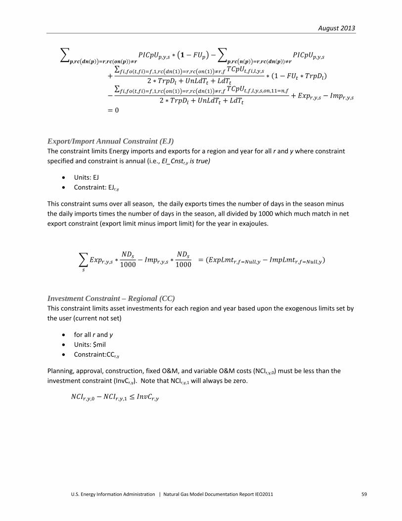
August 2013
U.S. Energy Information Administration | Natural Gas Model Documentation Report IEO2011 59
� 𝑃𝐼𝐶𝑝𝑈𝑝,𝑦,𝑠𝒑,𝒓𝒄�𝒅𝒏(𝒑)�=𝒓,𝒓𝒄(𝒐𝒏(𝒑))≠𝒓
∗ �𝟏 − 𝐹𝑈𝑝� −� 𝑃𝐼𝐶𝑝𝑈𝑝,𝑦,𝑠𝒑,𝒓𝒄�𝒏(𝒑)�=𝒓,𝒓𝒄(𝒅𝒏(𝒑))≠𝒓
+∑ 𝑇𝐶𝑝𝑈𝑡,𝑓𝑖,𝑙,𝑦,𝑠𝑓𝑖,𝑓𝑜(𝑡,𝑓𝑖)=𝑓,1,𝑟𝑐�𝑑𝑛(1)�=𝑟,𝑟𝑐�𝑜𝑛(1)�≠𝑟,𝑓
2 ∗ 𝑇𝑟𝑝𝐷𝑙 + 𝑈𝑛𝐿𝑑𝑇𝑡 + 𝐿𝑑𝑇𝑡∗ (1 − 𝐹𝑈𝑡 ∗ 𝑇𝑟𝑝𝐷𝑙)
−∑ 𝑇𝐶𝑝𝑈𝑡,𝑓,𝑙,𝑦,𝑠,𝑜𝑛,11=𝑛,𝑓𝑓𝑖,𝑓𝑜(𝑡,𝑓𝑖)=𝑓,1,𝑟𝑐�𝑜𝑛(1)�=𝑟,𝑟𝑐�𝑑𝑛(1)�≠𝑟,𝑓
2 ∗ 𝑇𝑟𝑝𝐷𝑙 + 𝑈𝑛𝐿𝑑𝑇𝑡 + 𝐿𝑑𝑇𝑡+ 𝐸𝑥𝑝𝑟,𝑦,𝑠 − 𝐼𝑚𝑝𝑟,𝑦,𝑠
= 0
Export/Import Annual Constraint (EJ) The constraint limits Energy imports and exports for a region and year for all r and y where constraint specified and constraint is annual (i.e., EI_Cnstr,y is true)
• Units: EJ • Constraint: EJr,y
This constraint sums over all season, the daily exports times the number of days in the season minus the daily imports times the number of days in the season, all divided by 1000 which much match in net export constraint (export limit minus import limit) for the year in exajoules.
�𝐸𝑥𝑝𝑟,𝑦,𝑠 ∗𝑁𝐷𝑠
1000− 𝐼𝑚𝑝𝑟,𝑦,𝑠 ∗
𝑁𝐷𝑠1000
𝑠
= (𝐸𝑥𝑝𝐿𝑚𝑡𝑟,𝑓=𝑁𝑢𝑙𝑙,𝑦 − 𝐼𝑚𝑝𝐿𝑚𝑡𝑟,𝑓=𝑁𝑢𝑙𝑙,𝑦)
Investment Constraint – Regional (CC) This constraint limits asset investments for each region and year based upon the exogenous limits set by the user (current not set)
• for all r and y • Units: $mil • Constraint:CCr,y
Planning, approval, construction, fixed O&M, and variable O&M costs (NCIr,y,0) must be less than the investment constraint (InvCr,y). Note that NCIr,y,1 will always be zero.
𝑁𝐶𝐼𝑟,𝑦,0 − 𝑁𝐶𝐼𝑟,𝑦,1 ≤ 𝐼𝑛𝑣𝐶𝑟,𝑦

August 2013
U.S. Energy Information Administration | Natural Gas Model Documentation Report IEO2011 60
Net Investment and O&M Costs – Regional (CI) This constraint is used to calculate the net investment costs for each region and year
• for all r and y • Units: $mil • Constraint:CIr,y
This constraint sums up costs minus revenues for each year y as follows:
• Adds up the planning and approval costs, construction costs, fixed operating and mainternace costs, and retirement costs for generic assets
• Adds the sum of asset planning and approval costs for assets started in previous year x that will have planning and approval costs in year y as follows: - PFa,x,y is 1 only if investments that start in year x for asset a has planning and approval
costs in year y - times PrCpEn,a,x which is the modelled capacity additions (PJ/day) - times PACsta which is the annual planning and approval cost for the capacity for a capacity
increment of CapIa ($mil/(PJ/day)) - divided by the capacity increment (PJ/day) - times the cost scalar (PScalar2,y)
• Adds the sum of asset construction costs for assets started in previous year x that will have construction costs in year y as follows: - CFa,x,y is 1 only if investments that start in year x for asset a has construction costs in year y - times PrCpEn,a,x which is the modelled capacity additions (PJ/day) - times ICsta which is the annual planning and approval cost for the capacity for a capacity
increment of CapIa ($mil/(PJ/day)) - divided by the capacity increment (PJ/day) - times the cost scalar (PScalar2,y)
• Adds the sum of asset fixed O&M costs for assets started in previous year x that will have construction costs in year y as follows: - OFa,x,y is 1 only if investments that start in year x for asset a is operational in year y - times PrCpEn,a,x which is the modelled capacity additions (PJ/day) - times FOaMCa which is the annual fixed O&M cost for the capacity for a capacity
increment of CapIa ($mil/(PJ/day)) - divided by the capacity increment (PJ/day) - times the cost scalar (PScalar2,y)
• Adds the sum of asset retirement costs for assets started in previous year x that will have retire in year y as follows: - RFa,x,y is 1 only if investments that start in year x for asset a retires in year y - times PrCpEn,a,x which is the modelled capacity additions (PJ/day) - times RCsta which is the retirement cost for the capacity for a capacity increment of CapIa
($mil/(PJ/day)) - divided by the capacity increment (PJ/day) - times the cost scalar (PScalar2,y)

August 2013
U.S. Energy Information Administration | Natural Gas Model Documentation Report IEO2011 61
• Adds the sum of variable O&M costs for assets that will operate in year y as follows: - PrCpUn,a,y,s which is the modelled capacity utilization of the asset type at the node in the
specified year and seasson (PJ/day) - times VOaMCa which is the variable operating cost for the ($/GJ output of primary
product) - times Qtya,f(a) which is the output fo the primary product (PJ/Day per CapIa of capacity) - divided by CapIa which is the input capacity used for costs and flows (PJ/day) - times the number of days in the seas (NDs) - times CGy which is the number of years in the year grouping - times the cost scalar (PScalar2,y)
• Adds up the planning and approval costs, construction costs, fixed operating and mainternace costs, and retirement costs for pipelines like above but - Using the pipeline capacity expansion starting planning approval in year x (PlCpEp,x) - Using the pipeline utilization (PlCpUp,y,s) - Time flags for the pipeline (PFp,x,y, …) - Simplifying the O&M costs calcualtions which do not need the flow (Qtya,f(a) and CapIa),
and - Using the price scalar for pipeline costs (PScalar1,y)
• Adds up the planning and approval costs, construction costs, fixed operating and mainternace costs, and retirement costs for tankers like above but - Using the tanker capacity expansion starting planning approval in year x (TCpEr,t,,x) - Using the tanker utilization (TCpUt,f,l,y,s) - Time flags for the tanker (PFt,x,y, …) - Simplifying the O&M costs calcualtions which do not need the flow (Qtya,f(a) and CapIa),
and - Using the price scalar for tanker costs (PScalar3,y)
• Adds up the planning and approval costs, construction costs, fixed operating and mainternace costs, and retirement costs for seasonal storage like above but - Using the storage capacity expansion starting planning approval in year x (SCpEn,g,x) - Using the storage injections (SCpIn,g,y,s) for the variable operating costs - Time flags for the storage (PFg,x,y, …) - Simplifying the O&M costs calcualtions which do not need the flow (Qtya,f(a) and CapIa),
and - Using the price scalar for storage costs (PScalar4,y)
• Subtracts the net cost variable (NCIr,y,1), and • Constrains the total to zero

August 2013
U.S. Energy Information Administration | Natural Gas Model Documentation Report IEO2011 62
� 𝑃𝐹𝑎,𝑥,𝑦𝑎𝑟(𝑛)=𝑟,𝑥
∗ 𝑃𝑟𝐶𝑝𝐸𝑛,𝑎,𝑥 ∗𝑃𝐴𝐶𝑠𝑡𝑎𝐶𝑎𝑝𝐼𝑎
∗ 𝑃𝑠𝑐𝑎𝑙𝑎𝑟2,𝑦 + � 𝐶𝐹𝑎.𝑥.𝑦𝑎,𝑟(𝑛)=𝑟,𝑥
∗ 𝑃𝑟𝐶𝑝𝐸𝑛,𝑎,𝑥 ∗𝐼𝐶𝑠𝑡𝑎𝐶𝑎𝑝𝐼𝑎
∗ 𝑃𝑠𝑐𝑎𝑙𝑎𝑟2,𝑦 + � 𝑂𝐹𝑎,𝑥,𝑦𝑎𝑟(𝑛)=𝑟,𝑥
∗ 𝑃𝑟𝐶𝑝𝐸𝑛,𝑎,𝑥 ∗𝐹𝑂𝑎𝑀𝐶𝑎𝐶𝑎𝑝𝐼𝑎
∗ 𝑃𝑠𝑐𝑎𝑙𝑎𝑟2,𝑦
+� 𝑅𝐹𝑎,𝑥,𝑦𝑎𝑟(𝑛)=𝑟,𝑥
∗ 𝑃𝑟𝐶𝑝𝐸𝑛,𝑎,𝑥 ∗𝑅𝐶𝑠𝑡𝑎𝐶𝑎𝑝𝐼𝑎
∗ 𝑃𝑠𝑐𝑎𝑙𝑎𝑟2,𝑦 + � 𝑃𝑟𝐶𝑝𝑈𝑛,𝑎,𝑦,𝑠𝑎𝑟(𝑛)=𝑟,𝑠
∗ 𝑉𝑂𝑎𝑀𝐶𝑎 ∗ 𝑄𝑡𝑦𝑎,𝑓(𝑎)𝑁𝐷𝑠 ∗ 𝐶𝐺𝑦𝐶𝑎𝑝𝐼𝑎
∗ 𝑃𝑠𝑐𝑎𝑙𝑎𝑟2,𝑦 + � 𝑃𝐹𝑝,𝑥,𝑦𝑝𝑟�𝑜𝑛(𝑝)�=𝑟,𝑥
∗ 𝑃𝑙𝐶𝑝𝐸𝑝,𝑥
∗𝑃𝐴𝐶𝑠𝑡𝑝𝐶𝑎𝑝𝐼𝑝
∗ 𝑃𝑠𝑐𝑎𝑙𝑎𝑟1,𝑦 + � 𝐶𝐹𝑝,𝑥,𝑦𝑝𝑟�𝑜𝑛(𝑝)�=𝑟,𝑥
∗ 𝑃𝑙𝐶𝑝𝐸𝑝,𝑥 ∗𝐼𝐶𝐶𝑠𝑡𝑝𝐶𝑎𝑝𝐼𝑝
∗ 𝑃𝑠𝑐𝑎𝑙𝑎𝑟1,𝑦
+� 𝑂𝐹𝑝,𝑥,𝑦𝑝𝑟�𝑜𝑛(𝑝)�=𝑟,𝑥
∗ 𝑃𝑙𝐶𝑝𝐸𝑝,𝑥 ∗𝐹𝑂𝑎𝑀𝐶𝑝𝐶𝑎𝑝𝐼𝑝
∗ 𝑃𝑠𝑐𝑎𝑙𝑎𝑟1,𝑦 +� 𝑅𝐹𝑝,𝑥,𝑦𝑝𝑟�𝑜𝑛(𝑝)�=𝑟,𝑥
∗ 𝑃𝑙𝐶𝑝𝐸𝑝,𝑥 ∗𝑅𝐶𝑠𝑡𝑝𝐶𝑎𝑝𝐼𝑝
∗ 𝑃𝑠𝑐𝑎𝑙𝑎𝑟1,𝑦 +� 𝑃𝐼𝐶𝑝𝑈𝑝,𝑦,𝑠𝑝𝑟�𝑜𝑛(𝑝)�=𝑟,𝑠
∗ 𝑉𝑂𝑎𝑀𝐶𝑝 ∗ 𝑁𝐷𝑠 ∗ 𝐶𝐺𝑦
∗ 𝑃𝑠𝑐𝑎𝑙𝑎𝑟1,𝑦 + � 𝑃𝐹𝑡,𝑥,𝑦𝑡,𝑥
∗ 𝑇𝑐𝑝𝐸𝑟,𝑡,𝑥 ∗𝑃𝐴𝐶𝑠𝑡𝑡𝐶𝑎𝑝𝐼𝑡
∗ 𝑃𝑆𝑐𝑎𝑙𝑎𝑟3,𝑦 + � 𝐶𝐹𝑡,𝑥,𝑦𝑡,𝑥
∗ 𝑇𝑐𝑝𝐸𝑟,𝑡,𝑥 ∗𝐼𝐶𝑠𝑡𝑡𝐶𝑎𝑝𝐼𝑡
∗ 𝑃𝑆𝑐𝑎𝑙𝑎𝑟3,𝑦 + � 𝑂𝐹𝑡,𝑥,𝑦𝑡,𝑥
∗ 𝑇𝑐𝑝𝐸𝑟,𝑡,𝑥 ∗𝐹𝑜𝑎𝑀𝐶𝑡𝑡𝐶𝑎𝑝𝐼𝑡
∗ 𝑃𝑆𝑐𝑎𝑙𝑎𝑟3,𝑦
+� 𝑅𝐹𝑡,𝑥,𝑦𝑡,𝑥
∗ 𝑇𝑐𝑝𝐸𝑟,𝑡,𝑥 ∗𝑅𝐶𝑠𝑡𝑡𝐶𝑎𝑝𝐼𝑡
∗ 𝑃𝑆𝑐𝑎𝑙𝑎𝑟3,𝑦 + � 𝑇𝐶𝑝𝑈𝑡,𝑓,𝑙,𝑦,𝑠𝑡,𝑓,;,𝑦�𝑜𝑛(1)�=𝑟
∗ 𝑉𝑂𝑎𝑀𝐶𝑡 ∗ 𝑁𝐷𝑠 ∗ 𝐶𝐺𝑦 ∗ 𝑃𝑆𝑐𝑎𝑙𝑎𝑟3,𝑦 + � 𝑃𝐹𝑔,𝑥,𝑦𝑎_𝑟(𝑛)=𝑟,𝑥
∗ 𝑆𝐶𝑝𝐸𝑛,𝑔,𝑥𝑃𝐴𝐶𝑠𝑡𝑔𝐶𝑎𝑝𝐼𝑔
∗ 𝑃𝑠𝑐𝑎𝑙𝑎𝑟4,𝑦 +� 𝐶𝐹𝑔,𝑥,𝑦𝑎_𝑟(𝑛)=𝑟,𝑥
∗ 𝑆𝐶𝑝𝐸𝑛,𝑔,𝑥𝐼𝐶𝐶𝑠𝑡𝑔𝐶𝑎𝑝𝐼𝑔
∗ 𝑃𝑠𝑐𝑎𝑙𝑎𝑟4,𝑦
+� 𝑂𝐹𝑔,𝑥,𝑦𝑎_𝑟(𝑛)=𝑟,𝑥
∗ 𝑆𝐶𝑝𝐸𝑛,𝑔,𝑥𝐹𝑂𝑎𝑚𝐶𝑔𝐶𝑎𝑝𝐼𝑔
∗ 𝑃𝑠𝑐𝑎𝑙𝑎𝑟4,𝑦 + � 𝑅𝐹𝑔,𝑥,𝑦𝑎_𝑟(𝑛)=𝑟,𝑥
∗ 𝑆𝐶𝑝𝐸𝑛,𝑔,𝑥𝑅𝐶𝑠𝑡𝑔𝐶𝑎𝑝𝐼𝑔
∗ 𝑃𝑠𝑐𝑎𝑙𝑎𝑟4,𝑦 + � 𝑆𝐶𝑝𝐼𝑛,𝑔,𝑦,𝑠𝑎_𝑟(𝑛)=𝑟,𝑠
∗ 𝑉𝑜𝑎𝑀𝐶𝑔 ∗ 𝑁𝐷𝑠
∗ 𝐶𝐺𝑦𝑃𝑠𝑐𝑎𝑙𝑎𝑟4,𝑦 − 𝑁𝐶𝐼𝑟,𝑦,𝑙 + 𝑁𝐶𝐼𝑟,𝑦,0 = 0
Capital constraint for other costs – regional (CO) This constraint is used to calculate the net operating costs for each region and year
• for all r and y • Units: $mil • Constraint:COr,y
This constraint is as follows
• The negative of the incremental daily demand scheduled from the demand curve price step (TDSn,k,i,y) is multiplied by the price of the step (DPrck,i) and number of years in the time group and converted to an annual cost. For this version ALfk is set to one, so the autoregressive component is one.

August 2013
U.S. Energy Information Administration | Natural Gas Model Documentation Report IEO2011 63
• Reserve adds (DRsn,c,j,y) times the adjusted resource extraction cost added. • Seasonal daily production (Prdn,c,m,y,s) is multiplied by the minimum of variable production costs
times the number of years in the time group, times the number of days in the season, and adjusted for government take but with the government take constrained to the government take percentage time $0.20/GJ, also with the prices scaled
• The revenue from other seasonal daily demand (ODn,f,y,s) times the price for the fuel and the number of days in the season and the number of years in time group I subtracted
• Plus the seasonal daily reinjected volumes times the reinjection cost times the number of days in the season and years in the time group, also times the operational cost price scalar
• Minus the variable for positive operational costs plus the variable for negative operational costs
−� 𝑻𝑫𝑺𝒏,𝒌,𝒊,𝒚𝒏,𝒌,𝒊,𝒓(𝒏)=𝒓
∗ 𝑫𝑷𝒓𝒄𝒌,𝒊 ∗ 𝟑𝟔𝟓.∗ 𝑪𝑮𝒚� [(𝟏 −𝟏
𝑨𝑳𝒇𝒌)�𝒚′−𝒚�
𝒚′≥𝒚,𝒀𝑮(𝒚′)=𝒚′
∗� 𝑫𝑹𝒂𝒕𝒆�𝒚′′−𝑺𝒚𝒆𝒂𝒓�𝒚′′,𝒈(𝒚′′)=𝒚′
]∑ 𝑫𝑹𝒂𝒕𝒆(𝒚′−𝑺𝒀𝒆𝒂𝒓)𝒚′,𝒈(𝒚′)=𝒚′
+ � 𝑫𝑹𝒔𝒏,𝒄,𝒋,𝒚𝒏,𝒄,𝒋,𝒎(𝒏,𝒄,𝒋)=𝒎,𝒓(𝒏)=𝒓
∗ 𝑺𝑷𝒓𝒄𝑨𝒏,𝒄,𝒋,𝒚 + � 𝑷𝒓𝒅𝒏,𝒄,𝒎,𝒚,𝒔𝒏,𝒄,𝒎,𝒓(𝒏)=𝒓
∗ 𝒎𝒊𝒏 �𝑽𝑷𝑪𝒏,𝒄,𝒎 ∗ 𝑪𝑮𝒚 ∗𝑵𝑫𝒔
𝟏 − 𝑮𝒐𝒗𝒕𝒏
∗ 𝑷𝒔𝒄𝒂𝒍𝒂𝒓𝟎,𝒚, �𝑽𝑷𝑪𝒏,𝒄,.𝒎 ∗ 𝑪𝑮𝒚 ∗ 𝑵𝑫𝒔 + 𝑮𝒐𝒗𝒕𝒏 ∗ 𝟎.𝟐� ∗ 𝑷𝒔𝒄𝒂𝒍𝒂𝒓𝒐,𝒚 �
−� 𝑶𝑫𝒏,𝒇,𝒚,𝒔𝒏,𝒇,𝒔,𝒓(𝒏)=𝒓
∗� 𝑶𝑷𝒓𝒄𝒇𝒇′𝒚𝒈(𝒚)=𝒚′
∗ 𝑵𝑫𝒔 + 𝑹𝑰𝑱𝒏,𝒄,𝒎=𝟎,𝒚,𝒔
∗𝑪𝑮𝒚 ∗ ∑𝒚′𝑺𝒀𝑮(𝒚′)=𝒚 �𝟎.𝟎𝟕𝟓 − 𝑶𝑷𝒓𝒄𝒇=𝑹𝑰𝑮,𝒚�𝑵𝑫𝒔
𝟏𝟎𝟎𝟎∗ 𝑷𝑺𝒄𝒂𝒍𝒂𝒓𝟎,𝒚 − 𝑵𝑪𝑶𝒓,𝒚,𝟏
+ 𝑵𝑪𝑶𝒓,𝒚,𝒐 = 𝟎
Average daily demand (ADD) This constraint sets the the natural gas demand quantity to be equal to the demand from the previous stock plus new demand using a autoregressive function of demand. Note that for now the variable ALfk is set to 1.
• for all n,k,y • Units: PJ/day • Constraint: ADDn,k,y
In the constraint the demand for the specified node, sector, and year is set to the demand in the previous time group YGP(y) times the reduction in demand due to the autoregressive coefficient (which for now is zero) plus the sum of the additional demand for the node, sector, and year by demand step.
𝑻𝑫𝒏,𝒌,𝒚 = 𝑻𝑫𝒏,𝒌,𝒀𝑮𝑷(𝒚) ∗ (𝟏 −𝟏
𝑨𝑳𝒇𝒌)(𝒚−𝒀𝑮𝑷(𝒚)) + � 𝑻𝑫𝑺𝒏,𝒌,𝒊,𝒚
𝒊
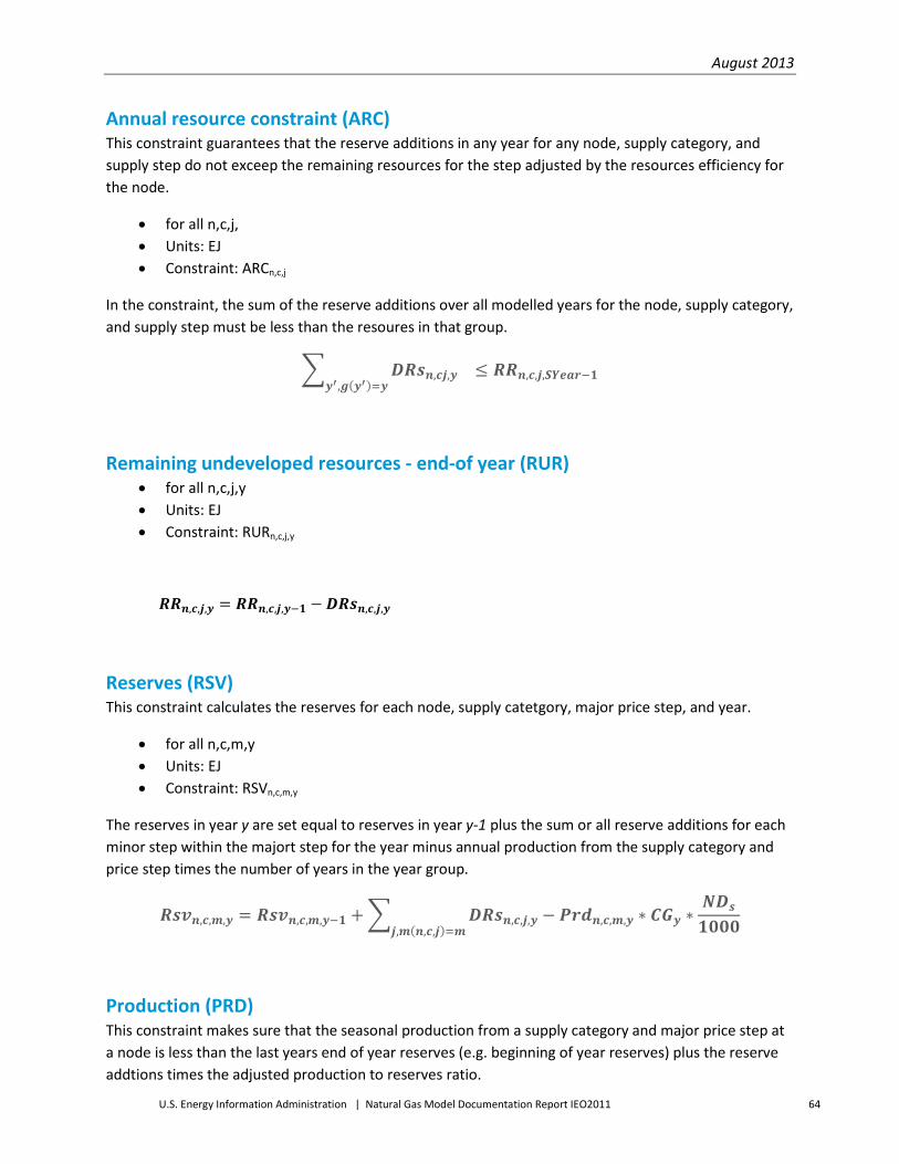
August 2013
U.S. Energy Information Administration | Natural Gas Model Documentation Report IEO2011 64
Annual resource constraint (ARC) This constraint guarantees that the reserve additions in any year for any node, supply category, and supply step do not exceep the remaining resources for the step adjusted by the resources efficiency for the node.
• for all n,c,j, • Units: EJ • Constraint: ARCn,c,j
In the constraint, the sum of the reserve additions over all modelled years for the node, supply category, and supply step must be less than the resoures in that group.
� 𝑫𝑹𝒔𝒏,𝒄𝒋,𝒚𝒚′,𝒈(𝒚′)=𝒚
≤ 𝑹𝑹𝒏,𝒄,𝒋,𝑺𝒀𝒆𝒂𝒓−𝟏
Remaining undeveloped resources - end-of year (RUR) • for all n,c,j,y • Units: EJ • Constraint: RURn,c,j,y
𝑹𝑹𝒏,𝒄,𝒋,𝒚 = 𝑹𝑹𝒏,𝒄,𝒋,𝒚−𝟏 − 𝑫𝑹𝒔𝒏,𝒄,𝒋,𝒚
Reserves (RSV) This constraint calculates the reserves for each node, supply catetgory, major price step, and year.
• for all n,c,m,y • Units: EJ • Constraint: RSVn,c,m,y
The reserves in year y are set equal to reserves in year y-1 plus the sum or all reserve additions for each minor step within the majort step for the year minus annual production from the supply category and price step times the number of years in the year group.
𝑹𝒔𝒗𝒏,𝒄,𝒎,𝒚 = 𝑹𝒔𝒗𝒏,𝒄,𝒎,𝒚−𝟏 + � 𝑫𝑹𝒔𝒏,𝒄,𝒋,𝒚𝒋,𝒎(𝒏,𝒄,𝒋)=𝒎
− 𝑷𝒓𝒅𝒏,𝒄,𝒎,𝒚 ∗ 𝑪𝑮𝒚 ∗𝑵𝑫𝒔
𝟏𝟎𝟎𝟎
Production (PRD) This constraint makes sure that the seasonal production from a supply category and major price step at a node is less than the last years end of year reserves (e.g. beginning of year reserves) plus the reserve addtions times the adjusted production to reserves ratio.

August 2013
U.S. Energy Information Administration | Natural Gas Model Documentation Report IEO2011 65
• for all n,c,m,y,s • Units: PJ/day • Constraint: PRDn,c,m,y,s
The constraint has the production less than or equal to the beginning of year reserves for the year group time PFac1 plus the total reserve additions for the year group times PFac2. Note that PFac1 accounts for the reserve depletion of the beginning of year reserves over all years in the year group using the PR ration and PFac2 accounts for the reserve additions being equally distributed to each year in the year group and reserve depletion for the reserve additions for all but the last year in the year group.
𝑷𝒓𝒅𝒏,𝒄,𝒎,𝒚,𝒔 ≤ 𝑹𝒔𝒗𝒏,𝒄,𝒎,𝒚−𝟏 ∗ 𝑷𝑭𝒂𝒄𝟏𝒏,𝒄,𝒎,𝒔 + �𝒋,𝒎(𝒏,𝒄,𝒋)=𝒎
𝑫𝑹𝒔𝒏,𝒄,𝒋,𝒚 ∗ 𝑷𝑭𝑨𝑪𝟐𝒏,𝒄,𝒎,𝒚
Pipeline asset capacity utilization (PCU) This constraint guarantees that the seasonal utilization of pipeline capacity in each year is less than or equal to the capacity existing or built as part of the optimization
• for all p, y, and s where sy+NYPp+NYCp ≤ y < EYp,sy+NYPp+NYCp+MxLp where there is a pipeline constraint at p,sy
• Units: PJ/Day • Constraint: PCUp,y,s
The sum of the capacity builds (PLCpEp,x) for the capacity investment years x where the capacity would be available for operation in year y (e.g., OFp,x,y = 1 and not 0) minus the pipeline utilization for the year and season must be greater than or equal to zero.
� 𝑶𝑭𝒑,𝒙,𝒚𝒙
∗ 𝑷𝑳𝑪𝒑𝑬𝒑,𝒙 − 𝑷𝑰𝑪𝒑𝑼𝒑,𝒚,𝒔 ≥ 𝟎
Pipeline capacity build constraints (PCG, PCL) These constraints limit the pipeline capacity additions to the range allowed by input data
• for all p and sy from pipeline asset constraints • Units: PJ/Day • Constraint: PCGp,sy
For each pipeline and capacity constraint identified by the start year of the constraint (sy), the sum of the capacity additions for year groups within the year range of the constraint must be greater than or equal to the minimum value allowed.

August 2013
U.S. Energy Information Administration | Natural Gas Model Documentation Report IEO2011 66
� 𝑷𝑳𝑪𝒑𝑬𝒑,𝒙𝒔𝒚≤𝒙≤𝑬𝒀𝒑,𝒔𝒚
≥ 𝑴𝒏𝑪𝒂𝒑𝒑,𝒔𝒚
• Constraint: PCLp,sy
For each pipeline and capacity constraint identified by the start year of the constraint (sy), the sum of the capacity additions for year groups within the year range of the constraint must be less than or equal to the maximum value allowed.
� 𝑷𝑳𝑪𝒑𝑬𝒑,𝒙𝒔𝒚≤𝒙≤𝑬𝒀𝒑,𝒔𝒚
≤ 𝑴𝒙𝑪𝒂𝒑𝒑,𝒔𝒚
Processing asset capacity utilization (ACU) This constraint guarantees that the seasonal utilization of processing asset capacity in each year is less than or equal to the capacity existing or built as part of the optimization
• for all n, a, y, and s where sy+NYPa+NYCa ≤ y < EYn,a,sy+NYPa+NYCa+MxLa where there is an asset constraint for n,a,sy
• Units: PJ/Day • Constraint ACUn,a,y,s
The sum of the capacity builds (PrCpEn,a,x) for the capacity investment years x where the capacity would be available for operation in year y (e.g., OFa,x,y = 1 and not 0) minus the processing asset utilization for the year and season must be greater than or equal to zero.
� 𝑶𝑭𝒂,𝒙,𝒚𝒙
∗ 𝑷𝒓𝑪𝒑𝑬𝒏,𝒂,𝒙 − 𝑷𝒓𝑪𝒑𝑼𝒏,𝒂,𝒚,𝒔 ≥ 𝟎
Processing asset capacity regional constraints (ACG, ACL) These constraints limit the processing capacity additions to the range allowed by input data
• for all n, a, and sy from processing asset regional constraints • Units: PJ/day • Constraint AGGn,a,y,s
For each processing asset, node, and capacity constraint identified by the start year of the constraint (sy), the sum of the capacity additions for year groups within the year range of the constraint must be greater than or equal to the minimum value allowed.
� 𝑷𝒓𝑪𝒑𝑬𝒏,𝒂𝒙𝒔𝒚≤𝒙≤𝑬𝒀𝒏,𝒂,𝒔𝒚
≥ 𝑴𝒏𝑪𝒂𝒑𝒏,𝒂,𝒔𝒚

August 2013
U.S. Energy Information Administration | Natural Gas Model Documentation Report IEO2011 67
Constraint AGLn,a,y,s For each processing asset, node, and capacity constraint identified by the start year of the constraint (sy), the sum of the capacity additions for year groups within the year range of the constraint must be less than or equal to the maximum value allowed.
� 𝑷𝒓𝑪𝒑𝑬𝒏,𝒂,𝒙𝒔𝒚≤𝒙≤𝑬𝒀𝒏,𝒂,𝒔𝒚
≥ 𝑴𝒙𝑪𝒂𝒑𝒏,𝒂,𝒔𝒚
Tanker asset capacity utilization (TCU) This constraint guarantees that the seasonal utilization of tanker asset capacity in each year is less than or equal to the capacity existing or built as part of the optimization
• for all r, t, y, and s where SYt,sy+NYPt+NYCt ≤ y ≤ EYt,sy+NYPt+NYCt+MxLt • Units: PJ Tanker Capacity • Constraint TCUr,t,y,s
The sum of the capacity builds (TcpEr,t,x) for the capacity investment years x where the capacity would be available for operation in year y (e.g., OFt,x,y = 1 and not 0) minus the tanker asset utilization for the year and season must be greater than or equal to zero.
� 𝑶𝑭𝒕,𝒙,𝒚𝒙
∗ 𝑻𝑪𝒑𝑬𝒓,𝒕,𝒙 −� 𝑻𝑪𝒑𝑼𝒕,𝒇𝒊,𝟏,𝒚,𝒔𝒇𝒊,𝟏,𝒓�𝒐𝒏(𝟏)�=𝒓
≥ 𝟎
Tanker capacity constraints (TCG, TCL) These constraints limit the tanker capacity additions to the range allowed by input data
• for all t and sy from tanker capacity constraints • Units: PJ/Day • Constraint TCGt,sy
For each tanker asset and capacity constraint identified by the start year of the constraint (sy), the sum of the capacity additions for year groups within the year range of the constraint must be greater than or equal to the minimum value allowed.
� 𝑻𝑪𝒑𝑬𝒓,𝒕,𝒙𝒓,𝒔𝒚≤𝒙≤𝑬𝒀𝒕,𝒔𝒚
≥ 𝑴𝒏𝑪𝒂𝒑𝒕,𝒔𝒚 ∗ 𝑪𝒂𝒑𝑰𝒕

August 2013
U.S. Energy Information Administration | Natural Gas Model Documentation Report IEO2011 68
Constraint TCLt,sy For each tanker asset and capacity constraint identified by the start year of the constraint (sy), the sum of the capacity additions for year groups within the year range of the constraint must be less than or equal to the maximum value allowed.
� 𝑻𝒄𝒑𝑬𝒓,𝒕,𝒙 ≤ 𝑴𝒙𝑪𝒂𝒑𝒕,𝒔𝒚𝒓,𝒔𝒚≤𝒙≤𝑬𝒀𝒕,𝒔𝒚
∗ 𝑪𝒂𝒑𝑰𝒕
Storage asset capacity utilization (SCU) This constraint guarantees that the seasonal utilization of storage asset capacity in each year is less than or equal to the capacity existing or built as part of the optimization
• for all n, g, and sy from storage asset regional constraints, and y where
𝑠𝑦 + 𝑁𝑌𝑃𝑔 ≤ 𝑦 < 𝐸𝑌𝑛,𝑔,𝑠𝑦 +𝑁𝑌𝑃𝑔 + 𝑁𝑌𝐶𝑔 + 𝑀𝑥𝐿𝑔
• Units: EJ • Constraint SCUn,g,y
The sum of the capacity builds (SCpEn,a,x) for the capacity investment years x where the capacity would be available for operation in year y (e.g., OFg,x,y = 1 and not 0) minus the storage asset injection volumes for the year and season must be greater than or equal to zero.
� 𝑂𝐹𝑔,𝑥,𝑦𝒙
∗ 𝑆𝐶𝑝𝐸𝑛,𝑔,𝑥 −� 𝑆𝐶𝑝𝐼𝑛,𝑔,𝑦,𝑠𝑠
∗ 𝑁𝐷𝑠 ≥ 0
Storage asset capacity regional constraints (SCG, SCL) These constraints limit the storage asset capacity additions to the range allowed by input data
• for all n, g, and sy from processing asset regional constraints • Units: EJ
Constraint SCGn,g,y,s For each storage asset and capacity constraint identified by the start year of the constraint (sy), the sum of the capacity additions for year groups within the year range of the constraint must be greater than or equal to the minimum value allowed.
� 𝑆𝐶𝑝𝐸𝑛,𝑔,𝑥𝒔𝒚≤𝒙≤𝐸𝑌𝑔,𝑠𝑦
≥ 𝑀𝑛𝐶𝑎𝑝𝐴𝑛,𝑔,𝑠𝑦

August 2013
U.S. Energy Information Administration | Natural Gas Model Documentation Report IEO2011 69
Constraint SCLn,g,y,s For each storage asset and capacity constraint identified by the start year of the constraint (sy), the sum of the capacity additions for year groups within the year range of the constraint must be less than or equal to the maximum value allowed.
� 𝑆𝐶𝑝𝐸𝑛,𝑔,𝑥𝒔𝒚≤𝒙≤𝐸𝑌𝑔,𝑠𝑦
≤ 𝑀𝑥𝐶𝑎𝑝𝐴𝑛,𝑔,𝑠𝑦
Storage asset volume balance (SCB) This constraint guarantees that the injection and withdrawal volumes match for each year
• for all n, a, sy from storage asset regional constraints, and y where
𝑠𝑦 +𝑁𝑌𝑃𝑔 + 𝑁𝑌𝐶𝑔 ≤ 𝑦 ≤ 𝐸𝑌𝑛,𝑎,𝑠𝑦 +𝑁𝑌𝑃𝑔 + 𝑁𝑌𝐶𝑔 + 𝑀𝑥𝐿𝑔
• Units: EJ • Constraint ACUn,g,y,s
The sum of the seasonal daily injection volumes times the number of days in the season times one minus the fuel use fraction, all minus the sum of the seasonal daily withdrawal volumes times the number of days in the season must equal to 0.
� 𝑆𝐶𝑝𝐼𝑛,𝑔,𝑦,𝑠𝑠
∗ 𝑁𝐷𝑠 ∗ �1 − 𝐹𝑈𝑔� −� 𝑆𝐶𝑝𝑊𝑛,𝑔,𝑦,𝑠𝑠
∗ 𝑁𝐷𝑠 = 0

August 2013
U.S. Energy Information Administration | Natural Gas Model Documentation Report IEO2011 70
Appendix A. Model Cost and Efficiency Assumptions A.1 Processing, liquefaction, regasification, and GTL asset specifications
Asset Name
Capacity
Increment FuelId
Num Yrs
PlnAppr PlanAppr Cst
Num Yrs
Investment
Investment
Cost
Maximum
Life
Fixed
O&M Cost
Variable
O&M Cost
Retirement
Cost
PJ/Day Years 2006
$MM/yr
Years 2006
$MM/yr
Years 2006
$MM/yr
2006 $/GJ 2006 $MM
Liquefaction Plant 1.0834 Processed LNG 3 102.2 3 2044 100 183.96 0.015 0
Small Regas Plant 0.5417 Processed
Natural Gas
3 11.4975 3 229.95 100 20.6955 0.123648 0
Large Regas Plant 1.0834 Processed
Natural Gas
3 19.1625 3 383.25 100 34.4925 0.123648 0
Large GTL Plant 0.37 Diesel (GTL) 3 20.64411 3 688.137 100 0 0.976 0
Small GTL Plant 0.184 Diesel (GTL) 3 16.09024 3 536.3413 100 0 0.976 0
Gas Processing Plant 0.4334 Processed
Natural Gas
3 1.3332 3 44.44 100 0 0.461 0
A.2 Plant efficiencies (output energy divided by input energy)
Asset Type Plant Efficiency
Gas Processing Plant 99.4%
Large GTL Plant 50.0%
Large Regas Plant 96.0%
Liquefaction Plant 92.0%
Small GTL Plant 50.0%
Small Regas Plant 96.0%

August 2013
U.S. Energy Information Administration | Natural Gas Model Documentation Report IEO2011 71
A.3 LNG tanker asset specifications
Tanker Name
Capacity Increment
Years Planning
and Approval
PlanAppr Cst
Years Investment
Investment Cost
Maximum Life
Fixed O&M Cost
Variable O&M
Cost Retirement
Cost ReGas
Cap Loading
Time Unloading
Time
PJ/Ship 2006
$MM/year 2006
$MM/year 2006
$MM/year 2006
$/GJ/day 2006$MM days days Small NoRegas 1.864 1 0.05 2 67.2535 40 0 0.038 0.05 Yes 1.85 1.85
Medium No Regas 2.984 1 0.05 3 56.5023 40 0 0.029 0.05 Yes 1.94 1.94 Large NoReGas 3.736 1 0.05 3 68.169 40 0 0.028 0.05 Yes 2.06 2.06
UltraLarge NoRegas 4.664 1 0.05 3 79.835 40 0 0.026 0.05 Yes 2.19 2.19

August 2013
U.S. Energy Information Administration | Natural Gas Model Documentation Report IEO2011 72
A.4 Pipeline specifications
Origin Node Dest. Node
Capacity Incre-ment
(PJ/day)
Years Planning
and Approval
Planning and
Approval Cost
($MM/yr)
Years Invest-
ment
Investment Cost
(2006$MM/yr)
Max Life
(years)
Fixed O&M Costs (2006
$MM/yr)
Variable O&M
Cost (2006
$MM/yr)
Fuel Use (%)
Retire-ment Cost
(2006 $MM)
Africa - North Africa - Rest 1.08 3 0.5 3 2978 100 0 0.412 8.25% 0.5
Africa - North Europe- South 1.08 3 0.5 3 1415 100 0 0.112 2.24% 0.5
Africa - North Europe- South West 1.08 3 0.5 3 1357 100 0 0.088 1.77% 0.5
Africa - North Rest of Middle East 1.08 3 0.5 3 1778 100 0 0.246 4.92% 0.5
Africa - Rest Africa - South 1.08 3 0.5 3 178 100 0 0.025 0.49% 0.5
Africa - West Africa - North 1.08 3 0.5 3 1257 100 0 0.174 3.48% 0.5 Africa - West Africa - Rest 1.08 3 0.5 3 2258 100 0 0.313 6.25% 0.5
Asia - Northwest India - North 1.08 3 0.5 3 276 100 0 0.038 0.76% 0.5 Asia - Other Developing SE China - West 1.08 3 0.5 3 1352 100 0 0.187 3.74% 0.5 Asia - Other Developing SE India - Southeast 1.08 3 0.5 3 610 100 0 0.084 1.69% 0.5
Asia - Producers Asia - Other Developed 1.08 3 0.5 3 523 100 0 0.072 1.45% 0.5
Australia and NZ - NW Shelf
Australia and NZ - Demand 1.08 3 0.5 3 2062 100 0 0.286 5.71% 0.5
Brazil
Latin America - Northern Producers 1.08 3 0.5 3 2692 100 0 0.373 7.46% 0.5
Canada East US - East North Central 1.08 3 0.5 3 603 100 0 0.084 1.67% 0.5
Canada East US - Middle Atlantic 1.08 3 0.5 3 315 100 0 0.044 0.87% 0.5
Canada East US - New England 1.08 3 0.5 3 294 100 0 0.041 0.81% 0.5
Canada East US - West North Central 1.08 3 0.5 3 874 100 0 0.121 2.42% 0.5
Canada West Canada East 1.08 3 0.5 3 1650 100 0 0.229 4.57% 0.5
Canada West US - Mountain 1.08 3 0.5 3 967 100 0 0.134 2.68% 0.5
Canada West US - Pacific Northwest 1.08 3 0.5 3 645 100 0 0.089 1.79% 0.5

August 2013
U.S. Energy Information Administration | Natural Gas Model Documentation Report IEO2011 73
A.4 Pipeline specifications (cont.)
Origin Node Dest. Node
Capacity Increment
(PJ/day)
Years Planning
and Approval
Planning and
Approval Cost
($MM/yr)
Years Invest-
ment
Investment Cost
(2006$MM/yr) Max Life
(years)
Fixed O&M Costs (2006
$MM/yr)
Variable O&M
Cost (2006
$MM/yr) Fuel Use
(%)
Retire-ment Cost
(2006 $MM)
Canada West US - West North Central 1.08 3 0.5 3 1154 100 0 0.16 3.20% 0.5
China - Northeast China - South 1.08 3 0.5 3 1100 100 0 0.152 3.05% 0.5 China - Northeast South Korea 1.08 3 0.5 3 554 100 0 0.077 1.54% 0.5
China - South Asia - Other Developed 1.08 3 0.5 3 554 100 0 0.077 1.54% 0.5
China - South China - Northeast 1.08 3 0.5 3 1100 100 0 0.152 3.05% 0.5 China - South China - West 1.08 3 0.5 3 762 100 0 0.106 2.11% 0.5 China - West Asia - Northwest 1.08 3 0.5 3 1977 100 0 0.274 5.48% 0.5 China - West China - South 1.08 3 0.5 3 762 100 0 0.106 2.11% 0.5 Europe- East Europe- North 1.08 3 0.5 3 966 100 0 0.134 2.68% 0.5 Europe- East Europe- South 1.08 3 0.5 3 981 100 0 0.136 2.72% 0.5 Europe- East Europe- Turkey 1.08 3 0.5 3 937 100 0 0.13 2.59% 0.5 Europe- East Russia West 1.08 3 0.5 3 1064 100 0 0.147 2.95% 0.5 Europe- North Europe- East 1.08 3 0.5 3 966 100 0 0.134 2.68% 0.5 Europe- North Europe- South 1.08 3 0.5 3 551 100 0 0.076 1.53% 0.5 Europe- North Europe- South West 1.08 3 0.5 3 771 100 0 0.107 2.14% 0.5 Europe- South Europe- East 1.08 3 0.5 3 981 100 0 0.136 2.72% 0.5 Europe- South Europe- North 1.08 3 0.5 3 551 100 0 0.076 1.53% 0.5 Europe- South West Europe- North 1.08 3 0.5 3 771 100 0 0.107 2.14% 0.5 Europe- Turkey Europe- East 1.08 3 0.5 3 937 100 0 0.13 2.59% 0.5 Europe- Turkey Europe- South 1.08 3 0.5 3 1137 100 0 0.157 3.15% 0.5 Europe- Turkey Rest of Middle East 1.08 3 0.5 3 388 100 0 0.054 1.07% 0.5 FSU Central Asia Asia - Northwest 1.08 3 0.5 3 740 100 0 0.102 2.05% 0.5 FSU Central Asia China - West 1.08 3 0.5 3 2348 100 0 0.325 6.50% 0.5 FSU Central Asia Europe- East 1.08 3 0.5 3 1838 100 0 0.255 5.09% 0.5 FSU Central Asia Europe- Turkey 1.08 3 0.5 3 1526 100 0 0.211 4.23% 0.5

August 2013
U.S. Energy Information Administration | Natural Gas Model Documentation Report IEO2011 74
A.4 Pipeline specifications (cont.)
Origin Node Dest. Node
Capacity Incre-ment
(PJ/day)
Years Planning
and Approval
Planning and
Approval Cost
($MM/yr)
Years Invest-
ment
Investment Cost
(2006$MM/yr)
Max Life
(years)
Fixed O&M Costs (2006
$MM/yr)
Variable O&M
Cost (2006
$MM/yr) Fuel
Use (%)
Retire-ment Cost
(2006 $MM)
FSU Central Asia Iran 1.08 3 0.5 3 918 100 0 0.127 2.54% 0.5
FSU Central Asia Russia Caspian Sea 1.08 3 0.5 3 1102 100 0 0.153 3.05% 0.5
FSU Central Asia Russia West 1.08 3 0.5 3 1627 100 0 0.225 4.51% 0.5
India - Southeast India - Southwest 1.08 3 0.5 3 279 100 0 0.072 1.44% 0.5
India - Southwest India - North 1.08 3 0.5 3 521 100 0 0.072 1.44% 0.5
Iran Europe- Turkey 1.08 3 0.5 3 1606 100 0 0.222 4.45% 0.5
Iran FSU Central Asia 1.08 3 0.5 3 918 100 0 0.127 2.54% 0.5
Iraq Arabian Producers 1.08 3 0.5 3 45 100 0 0.065 15.00% 0.2
Iraq Europe- Turkey 1.08 3 0.5 3 842 100 0 0.117 2.33% 0.5
Iraq Rest of Middle East 1.08 3 0.5 3 187 100 0 0.026 0.52% 0.5
Latin America - Andean Brazil 1.08 3 0.5 3 2297 100 0 0.318 6.36% 0.5
Latin America - Andean Latin America - Southern Cone 1.08 3 0.5 3 1829 100 0 0.253 5.07% 0.5
Latin America - Central America US - Florida 1.08 3 0.5 3 975 100 0 0.135 2.70% 0.5 Latin America - Northern Producers Brazil 1.08 3 0.5 3 2692 100 0 0.373 7.46% 0.5 Latin America - Northern Producers
Latin America - Central America 1.08 3 0.5 3 1063 100 0 0.147 2.95% 0.5
Latin America - Southern Cone Brazil 1.08 3 0.5 3 1276 100 0 0.177 3.53% 0.5
Latin America - Southern Cone Chile 1.08 3 0.5 3 717 100 0 0.099 1.99% 0.5
Mexico Northeast US - West South Central 1.08 3 0.5 3 499 100 0 0.069 1.38% 0.5
Mexico Northwest Mexico Northeast 1.08 3 0.5 3 648 100 0 0.09 1.80% 0.5
Mexico Northwest US - AZNM 1.08 3 0.5 3 289 100 0 0.04 0.80% 0.5
Mexico Northwest US - California 1.08 3 0.5 3 501 100 0 0.069 1.39% 0.5 Mexico South Mexico Northeast 1.08 3 0.5 3 413 100 0 0.057 1.14% 0.5

August 2013
U.S. Energy Information Administration | Natural Gas Model Documentation Report IEO2011 75
A.4 Pipeline specifications (cont.)
Origin Node Dest. Node
Capacity Incre-ment
(PJ/day)
Years Planning
and Approval
Planning and
Approval Cost
($MM/yr)
Years Invest-
ment
Investment Cost
(2006$MM/yr)
Max Life
(years)
Fixed O&M Costs (2006
$MM/yr)
Variable O&M
Cost (2006
$MM/yr) Fuel
Use (%)
Retire-ment Cost
(2006 $MM)
Mexico Southwest LNG Mexico South 1.08 3 0.5 3 292 100 0 0.04 0.81% 0.5 Qatar Arabian Producers 1.08 3 0.5 3 557 100 0 0.077 1.54% 0.5
Rest of Middle East Europe- Turkey 1.08 3 0.5 3 388 100 0 0.054 1.07% 0.5
Russia Caspian Sea Europe- Turkey 1.08 3 0.5 3 548 100 0 0.076 1.52% 0.5
Russia Caspian Sea FSU Central Asia 1.08 3 0.5 3 1102 100 0 0.153 3.05% 0.5
Russia Caspian Sea Russia West 1.08 3 0.5 3 1102 100 0 0.153 3.05% 0.5
Russia East China - Northeast 1.08 3 0.5 3 999 100 0 0.138 2.77% 0.5
Russia East China - West 1.08 3 0.5 3 2874 100 0 0.398 7.96% 0.5
Russia East Russia Sakhalin 1.08 3 0.5 3 2874 100 0 0.398 7.96% 0.5
Russia East Russia West 1.08 3 0.5 3 2874 100 0 0.398 7.96% 0.5
Russia Sakhalin China - Northeast 1.08 3 0.5 3 999 100 0 0.138 2.77% 0.5
Russia Sakhalin Russia East 1.08 3 0.5 3 647 100 0 0.09 1.79% 0.5
Russia Shtokman Russia West 1.08 3 0.5 3 635 100 0 0.088 1.76% 0.5
Russia West China - West 1.08 3 0.5 3 1726 100 0 0.398 7.96% 0.5
Russia West Europe- East 1.08 3 0.5 3 1064 100 0 0.147 2.95% 0.5
Russia West Europe- North 1.08 3 0.5 3 1864 100 0 0.258 5.16% 0.5
Russia West Russia Caspian Sea 1.08 3 0.5 3 1102 100 0 0.153 3.05% 0.5
Russia West Russia East 1.08 3 0.5 3 2874 100 0 0.398 7.96% 0.5
Russia Yamal Russia West 1.08 3 0.5 3 575 100 0 0.08 1.59% 0.5
US - Arctic Canada West 1.08 3 0.5 3 1476 100 0 0.204 4.09% 0.5
US - AZNM Mexico Northwest 1.08 3 0.5 3 289 100 0 0.04 0.80% 0.5
US - AZNM US - California 1.08 3 0.5 3 330 100 0 0.046 0.92% 0.5
US - AZNM US - Mountain 1.08 3 0.5 3 548 100 0 0.076 1.52% 0.5
US - AZNM US - West South Central 1.08 3 0.5 3 828 100 0 0.115 2.29% 0.5

August 2013
U.S. Energy Information Administration | Natural Gas Model Documentation Report IEO2011 76
A.4 Pipeline specifications (cont.)
Origin Node Dest. Node
Capacity Incre-ment
(PJ/day)
Years Planning
and Approval
Planning and
Approval Cost
($MM/yr)
Years Invest-
ment
Investment Cost
(2006$MM/yr)
Max Life
(years)
Fixed O&M Costs (2006
$MM/yr)
Variable O&M
Cost (2006
$MM/yr) Fuel
Use (%)
Retire-ment Cost
(2006 $MM)
US - California Mexico Northwest 1.08 3 0.5 3 501 100 0 0.069 1.39% 0.5
US - California US - AZNM 1.08 3 0.5 3 330 100 0 0.046 0.92% 0.5
US - California US - Mountain 1.08 3 0.5 3 784 100 0 0.109 2.17% 0.5
US - East North Central Canada East 1.08 3 0.5 3 603 100 0 0.084 1.67% 0.5
US - East North Central US - East South Central 1.08 3 0.5 3 631 100 0 0.087 1.75% 0.5
US - East North Central US - Middle Atlantic 1.08 3 0.5 3 666 100 0 0.092 1.84% 0.5
US - East North Central US - South Atlantic 1.08 3 0.5 3 551 100 0 0.076 1.53% 0.5
US - East North Central US - West North Central 1.08 3 0.5 3 290 100 0 0.04 0.80% 0.5
US - East South Central US - East North Central 1.08 3 0.5 3 631 100 0 0.087 1.75% 0.5
US - East South Central US - Florida 1.08 3 0.5 3 640 100 0 0.089 1.77% 0.5
US - East South Central US - South Atlantic 1.08 3 0.5 3 328 100 0 0.045 0.91% 0.5
US - East South Central US - West South Central 1.08 3 0.5 3 361 100 0 0.05 1.00% 0.5
US - Middle Atlantic Canada East 1.08 3 0.5 3 315 100 0 0.044 0.87% 0.5
US - Middle Atlantic US - East North Central 1.08 3 0.5 3 666 100 0 0.092 1.84% 0.5
US - Middle Atlantic US - New England 1.08 3 0.5 3 178 100 0 0.025 0.49% 0.5
US - Middle Atlantic US - South Atlantic 1.08 3 0.5 3 699 100 0 0.097 1.93% 0.5
US - Mountain Canada West 1.08 3 0.5 3 967 100 0 0.134 2.68% 0.5
US - Mountain US - AZNM 1.08 3 0.5 3 548 100 0 0.076 1.52% 0.5
US - Mountain US - California 1.08 3 0.5 3 784 100 0 0.109 2.17% 0.5
US - Mountain US - Pacific Northwest 1.08 3 0.5 3 918 100 0 0.127 2.54% 0.5
US - Mountain US - West North Central 1.08 3 0.5 3 570 100 0 0.079 1.58% 0.5

August 2013
U.S. Energy Information Administration | Natural Gas Model Documentation Report IEO2011 77
A.4 Pipeline specifications (cont.)
Origin Node Dest. Node
Capacity Incre-ment
(PJ/day)
Years Planning
and Approval
Planning and
Approval Cost
($MM/yr)
Years Invest-
ment
Investment Cost
(2006$MM/yr)
Max Life
(years)
Fixed O&M Costs (2006
$MM/yr)
Variable O&M
Cost (2006
$MM/yr) Fuel
Use (%)
Retire-ment Cost
(2006 $MM)
US - Mountain US - West South Central 1.08 3 0.5 3 620 100 0 0.086 1.72% 0.5
US - New England Canada East 1.08 3 0.5 3 294 100 0 0.041 0.81% 0.5
US - New England US - Middle Atlantic 1.08 3 0.5 3 178 100 0 0.025 0.49% 0.5 US - Pacific Northwest Canada West 1.08 3 0.5 3 645 100 0 0.089 1.79% 0.5
US - Pacific Northwest US - California 1.08 3 0.5 3 792 100 0 0.11 2.19% 0.5
US - Pacific Northwest US - Mountain 1.08 3 0.5 3 918 100 0 0.127 2.54% 0.5
US – South Atlantic US – East North Central 1.083485 3 0.5 3 551 100 0 0.076365 1.53% 0.5
US – South Atlantic US – East South Central 1.083485 3 0.5 3 328 100 0 0.045454 0.91% 0.5
US – South Atlantic US – Florida 1.083485 3 0.5 3 509 100 0 0.070429 1.41% 0.5
US – South Atlantic US – Middle Atlantic 1.083485 3 0.5 3 699 100 0 0.096731 1.93% 0.5
US – West North Central Canada East 1.083485 3 0.5 3 874 100 0 0.121078 2.42% 0.5
US – West North Central US – East North Central 1.083485 3 0.5 3 290 100 0 0.040102 0.80% 0.5
US – West North Central US – Moiuntain 1.083485 3 0.5 3 570 100 0 0.078985 1.58% 0.5
US – West North Central US – West South Central 1.083485 3 0.5 3 593 100 0 0.082102 1.64% 0.5
US – West South Central Mexico Northeast 1.083485 3 0.5 3 499 100 0 0.069116 1.38% 0.5
US – West South Central US - AZNM 1.083485 3 0.5 3 828 100 0 0.114632 2.29% 0.5
US – West South Central US – East South Central 1.083485 3 0.5 3 361 100 0 0.049961 1.00% 0.5
US – West South Central US – Mountain 1.083485 3 0.5 3 620 100 0 0.085842 1.72% 0.5
US – West South Central US –West North Central 1.083485 3 0.5 3 593 100 0 0.082102 1.64% 0.5

August 2013
U.S. Energy Information Administration | Natural Gas Model Documentation Report IEO2011 78
A.5 Storage asset specifications
Capacity Increment (EJ of Working Gas)
Years Planning and Approval
Planning and Approval Cost
($MM/yr) Years
Invest-ment
Investment Cost
(2006$MM/yr) Max Life
(years)
Fixed O&M Costs (2006
$MM/yr)
Variable O&M Cost
(2006 $MM/yr)
Fuel Use (%)
Fuel Use (%)
230.4171 2 12.81 3 426.95 100 0 0.185 0.1 5.00%
A.6 Demand sector price elasticities
tInp_DmdSector
DmdSector Name Price Elasticity for
Iterative Runs Price Elasticity for
Final Fun
Residential -0.87971 -0.031
Commercial -0.9 -0.032
Transportation -1 -0.033
Industrial Cogen -1 -0.05
Industrial Feedstock -0.92017 -0.05
Other Industrial -0.6646 -0.05
Power Generation -1 -0.055
Reinjection -0.0001 -0.0001

August 2013
U.S. Energy Information Administration | Natural Gas Model Documentation Report IEO2011 79
A.7 Mapping from INGM nodes to WEPS+regions
tInp_Node_Scn
NodeId RegionId
Africa - North Africa
Africa - Rest Africa
Africa - South Africa
Africa - West Africa
Arabian Producers Middle East
Asia - Northwest Other Asia
Asia - Other Developed Other Asia
Asia - Other Developing SE Other Asia
Asia - Producers Other Asia
Australia and NZ - Demand Australia & New-Zealand
Australia and NZ - NW Shelf Australia & New-Zealand
Brazil Brazil
Canada East Canada
Canada West Canada
Chile Chile
China - Northeast China
China - South China
China - West China
Europe- East Non-OECD Europe and Eurasia
Europe- North OECD Europe
Europe- South OECD Europe
Europe- South West OECD Europe
Europe- Turkey OECD Europe
FSU Central Asia Non-OECD Europe and Eurasia
India - North India
India - Southeast India
India - Southwest India
Iran Middle East
Iraq Middle East
Japan Japan
Latin America - Andean Non-OECD Americas
Latin America - Central America Non-OECD Americas
Latin America - Northern Producers Non-OECD Americas

August 2013
U.S. Energy Information Administration | Natural Gas Model Documentation Report IEO2011 80
A.7 Mapping from INGM nodes to WEPS+regions (cont.)
tInp_Node_Scn
NodeId RegionId
Latin America - Southern Cone Non-OECD Americas
Mexico Northeast Mexico
Mexico Northwest Mexico
Mexico South Mexico
Mexico Southwest LNG Mexico
Qatar Middle East
Rest of Middle East Middle East
Russia Caspian Sea Russia
Russia East Russia
Russia Sakhalin Russia
Russia Shtokman Russia
Russia West Russia
Russia Yamal Russia
Saudi Arabia Middle East
South Korea South Korea
US - Arctic United States
US - AZNM United States
US - California United States
US - East North Central United States
US - East South Central United States
US - Florida United States
US - Middle Atlantic United States
US - Mountain United States
US - New England United States
US - Pacific Northwest United States
US - South Atlantic United States
US - West North Central United States
US - West South Central United States

August 2013
U.S. Energy Information Administration | Natural Gas Model Documentation Report IEO2011 81
Appendix B Capacity Assumptions for Processing, Conversion, and Transporation Assets B.1 Processing, liquefaction, regasification, and gtl asset nodal constraints
Node Asset First Year Available
Last Year Available
Minimum Capacity
Build
Maximum Capacity
Build
Africa - North Gas Processing Plant 2006 2006 16.203 999999
Africa - North Gas Processing Plant 2007 2060 0 999999
Africa - North Liquefaction Plant 2006 2006 4.334628 4.334628
Africa - North Liquefaction Plant 2012 2013 0.645943 0.98953
Africa - North Liquefaction Plant 2014 2015 0.645943 1.126965
Africa - North Liquefaction Plant 2016 2060 0 999999
Africa - Rest Gas Processing Plant 2006 2060 0 999999
Africa - Rest Liquefaction Plant 2016 2060 0 999999
Africa - South Gas Processing Plant 2006 2060 0 999999
Africa - South Small GTL Plant 2007 2007 0.276 0.276
Africa - South Small GTL Plant 2012 2012 0.0138 0.0138
Africa - South Small GTL Plant 2013 2013 0.01449 0.01449
Africa - South Small GTL Plant 2014 2014 0.015215 0.015215
Africa - South Small GTL Plant 2015 2015 0.009585 0.009585
Africa - South Small GTL Plant 2016 2020 0.00831 0.00831
Africa - South Small GTL Plant 2021 2025 0.00852 0.00852
Africa - South Small GTL Plant 2026 2030 0.008735 0.008735
Africa - South Small GTL Plant 2031 2035 0.008955 0.008955
Africa - South Small GTL Plant 2036 2040 0.008955 0.008955
Africa - South Small Regas Plant 2016 2060 0 999999
Africa - West Gas Processing Plant 2006 2006 2.54 999999
Africa - West Gas Processing Plant 2007 2060 0 999999
Africa - West Liquefaction Plant 2008 2008 2.241171 2.241171
Africa - West Liquefaction Plant 2010 2010 0.518324 0.518324
Africa - West Liquefaction Plant 2011 2011 0.518324 0.518324
Africa - West Liquefaction Plant 2012 2012 0.35733 0.35733
Africa - West Liquefaction Plant 2013 2013 0.35733 0.35733
Africa - West Liquefaction Plant 2016 2060 0 999999
Africa - West Small GTL Plant 2013 2013 0.1045 0.1045
Africa - West Small GTL Plant 2014 2014 0.1045 0.1045

August 2013
U.S. Energy Information Administration | Natural Gas Model Documentation Report IEO2011 82
B.1 Processing, liquefaction, regasification, and gtl asset nodal constraints (cont.)
Node Asset First Year Available
Last Year Available
Minimum Capacity
Build
Maximum Capacity
Build
Arabian Producers Gas Processing Plant 2006 2006 4.688 999999
Arabian Producers Gas Processing Plant 2007 2060 0 999999
Arabian Producers Liquefaction Plant 2006 2006 1.553013 1.553013
Arabian Producers Liquefaction Plant 2009 2009 0.460406 0.460406
Arabian Producers Liquefaction Plant 2010 2010 0.460406 0.460406
Arabian Producers Liquefaction Plant 2116 2160 0 999999
Arabian Producers Small Regas Plant 2009 2009 0.180229 0.180229
Arabian Producers Small Regas Plant 2010 2010 0.765974 0.765974
Arabian Producers Small Regas Plant 2011 2011 0.135172 0.135172
Arabian Producers Small Regas Plant 2015 2060 0 999999
Asia - Northwest Gas Processing Plant 2006 2006 1.298 999999
Asia - Northwest Gas Processing Plant 2007 2060 0 999999
Asia - Northwest Small Regas Plant 2012 2013 0 0.481022
Asia - Northwest Small Regas Plant 2014 2015 0 0.481022
Asia - Northwest Small Regas Plant 2016 2060 0 1032289
Asia - Other Developed Gas Processing Plant 2006 2060 0 999999
Asia - Other Developed Small Regas Plant 2006 2006 1.085735 1.085735
Asia - Other Developed Small Regas Plant 2008 2008 0.206152 0.206152
Asia - Other Developed Small Regas Plant 2009 2009 0.206152 0.206152
Asia - Other Developed Small Regas Plant 2012 2014 0 0.412304
Asia - Other Developed Small Regas Plant 2015 2060 0 999999 Asia - Other Developing SE
Gas Processing Plant 2006 2006 1.503 999999
Asia - Other Developing SE
Gas Processing Plant 2007 2060 0 999999
Asia - Other Developing SE Liquefaction Plant 2012 2013 0.233639 0.371074
Asia - Other Developing SE Liquefaction Plant 2014 2015 0 1.965317
Asia - Other Developing SE Liquefaction Plant 2016 2060 0 999999
Asia - Other Developing SE Small Regas Plant 2012 2014 0 0.687174
Asia - Other Developing SE Small Regas Plant 2015 2060 0 999999

August 2013
U.S. Energy Information Administration | Natural Gas Model Documentation Report IEO2011 83
B.1 Processing, liquefaction, regasification, and gtl asset nodal constraints (cont.)
Node Asset First Year Available
Last Year Available
Minimum Capacity
Build
Maximum Capacity
Build
Asia - Producers Gas Processing Plant 2006 2006 13.963 999999
Asia - Producers Gas Processing Plant 2007 2060 0 999999
Asia - Producers Liquefaction Plant 2006 2006 7.160351 7.160351
Asia - Producers Liquefaction Plant 2008 2008 0.522252 0.522252
Asia - Producers Liquefaction Plant 2009 2009 0.522252 0.522252
Asia - Producers Liquefaction Plant 2010 2010 0 0.137435
Asia - Producers Liquefaction Plant 2011 2015 0 0.824609
Asia - Producers Liquefaction Plant 2016 2060 0 999999
Asia - Producers Small GTL Plant 2001 2001 0.09 0.09
Asia - Producers Small Regas Plant 2012 2014 0.206152 0.412304
Asia - Producers Small Regas Plant 2015 2060 0 999999
Australia and NZ - Demand
Gas Processing Plant 2006 2060 0 999999
Australia and NZ - Demand Liquefaction Plant 2015 2015 0 0.470115
Australia and NZ - Demand Liquefaction Plant 2016 2016 0 0.470115
Australia and NZ - Demand Liquefaction Plant 2017 2017 0 0.470115
Australia and NZ - Demand Liquefaction Plant 2018 2018 0 0.470115
Australia and NZ - Demand Liquefaction Plant 2019 2019 0 0.470115
Australia and NZ - Demand Liquefaction Plant 2020 2020 0 0.470115
Australia and NZ - Demand Liquefaction Plant 2021 2021 0 0.470115 Australia and NZ - Demand Liquefaction Plant 2022 2022 0 0.470115
Australia and NZ - Demand Liquefaction Plant 2023 2023 0 0.470115
Australia and NZ - Demand Liquefaction Plant 2024 2024 0 0.470115
Australia and NZ - Demand Liquefaction Plant 2025 2025 0 0.183246
Australia and NZ - Demand Liquefaction Plant 2026 2026 0 0.183246

August 2013
U.S. Energy Information Administration | Natural Gas Model Documentation Report IEO2011 84
B.1 Processing, liquefaction, regasification, and gtl asset nodal constraints (cont.)
Node Asset First Year Available
Last Year Available
Minimum Capacity
Build
Maximum Capacity
Build
Australia and NZ - Demand Liquefaction Plant 2027 2027 0 0.183246
Australia and NZ - Demand Liquefaction Plant 2028 2028 0 0.183246
Australia and NZ - Demand Liquefaction Plant 2029 2029 0 0.183246
Australia and NZ - Demand Liquefaction Plant 2030 2030 0 0.183246 Australia and NZ - Demand Liquefaction Plant 2031 2031 0 0.183246
Australia and NZ - Demand Liquefaction Plant 2032 2032 0 0.183246
Australia and NZ - Demand Liquefaction Plant 2033 2033 0 0.183246
Australia and NZ - Demand Liquefaction Plant 2034 2034 0 0.183246
Australia and NZ - Demand Liquefaction Plant 2035 2035 0 0.183246 Australia and NZ - Demand Liquefaction Plant 2036 2036 0 0.183246
Australia and NZ - Demand Liquefaction Plant 2037 2037 0 0.183246
Australia and NZ - Demand Liquefaction Plant 2038 2038 0 0.183246
Australia and NZ - Demand Liquefaction Plant 2039 2039 0 0.183246
Australia and NZ - Demand Liquefaction Plant 2040 2040 0 0.183246
Australia and NZ - Demand Liquefaction Plant 2041 2041 0 0.183246
Australia and NZ - Demand Small Regas Plant 2012 2014 0 0.412304 Australia and NZ - Demand Small Regas Plant 2015 2060 0 999999
Australia and NZ - NW Shelf
Gas Processing Plant 2006 2006 4.763 999999
Australia and NZ - NW Shelf
Gas Processing Plant 2007 2060 0 999999
Australia and NZ - NW Shelf Liquefaction Plant 2006 2006 1.889728 1.889728
Australia and NZ - NW Shelf Liquefaction Plant 2007 2007 0.240511 0.240511 Australia and NZ - NW Shelf Liquefaction Plant 2008 2008 0.201571 0.201571

August 2013
U.S. Energy Information Administration | Natural Gas Model Documentation Report IEO2011 85
B.1 Processing, liquefaction, regasification, and gtl asset nodal constraints (cont.)
Node Asset First Year Available
Last Year Available
Minimum Capacity
Build
Maximum Capacity
Build
Australia and NZ - NW Shelf Liquefaction Plant 2009 2009 0.403142 0.403142
Australia and NZ - NW Shelf Liquefaction Plant 2010 2010 0 0
Australia and NZ - NW Shelf Liquefaction Plant 2011 2011 0.439791 0.439791
Australia and NZ - NW Shelf Liquefaction Plant 2012 2012 0.219896 0.219896 Australia and NZ - NW Shelf Liquefaction Plant 2013 2013 0 0
Australia and NZ - NW Shelf Liquefaction Plant 2014 2014 0.229058 0.229058
Australia and NZ - NW Shelf Liquefaction Plant 2015 2015 0.687174 0.687174
Australia and NZ - NW Shelf Liquefaction Plant 2016 2016 0.687174 0.687174
Australia and NZ - NW Shelf Liquefaction Plant 2017 2017 0.458116 1.787797 Australia and NZ - NW Shelf Liquefaction Plant 2018 2060 0 999999
Brazil Gas Processing Plant 2006 2006 1.177 999999
Brazil Gas Processing Plant 2007 2060 0 999999
Brazil Liquefaction Plant 2025 2027 0 0.1649
Brazil Liquefaction Plant 2028 2030 0 0.1649
Brazil Liquefaction Plant 2031 2033 0 0.1649
Brazil Liquefaction Plant 2034 2036 0 0.1649
Brazil Liquefaction Plant 2037 2039 0 0.1649
Brazil Liquefaction Plant 2040 2042 0 0.1649
Brazil Liquefaction Plant 2043 2045 0 0.1649
Brazil Liquefaction Plant 2046 2048 0 0.1649
Brazil Liquefaction Plant 2049 2051 0 0.1649
Brazil Liquefaction Plant 2052 2054 0 0.1649
Brazil Small Regas Plant 2009 2009 0.886454 0.886454
Brazil Small Regas Plant 2010 2010 0.364202 0.364202
Brazil Small Regas Plant 2011 2014 0.522252 1.250656
Brazil Small Regas Plant 2015 2060 0 999999
Canada East Gas Processing Plant 2006 2006 0.652 999999
Canada East Gas Processing Plant 2007 2060 0 999999
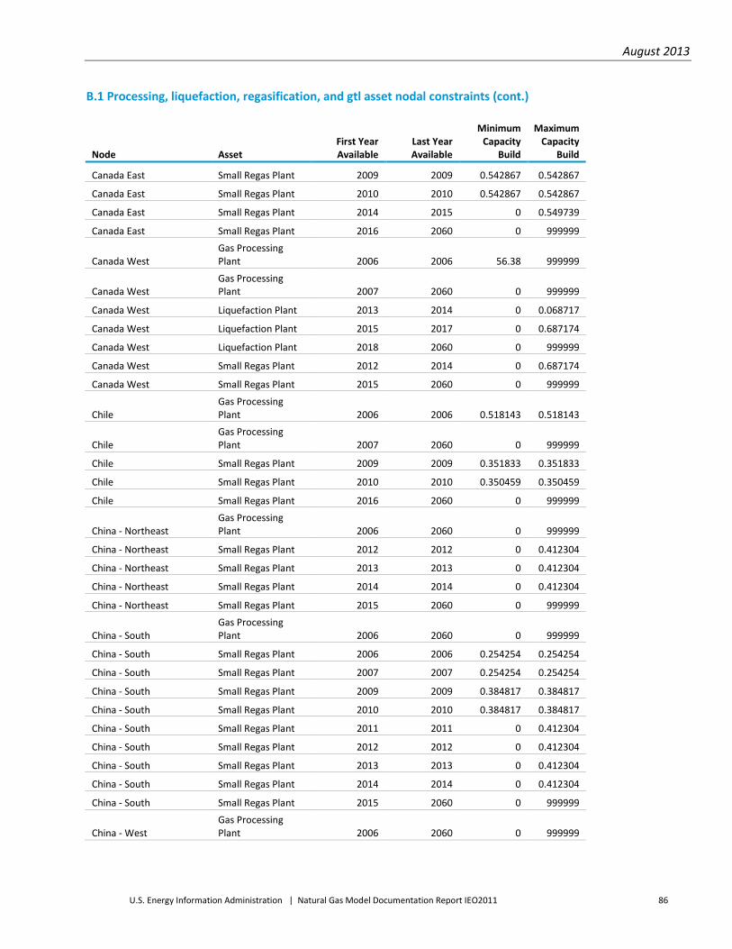
August 2013
U.S. Energy Information Administration | Natural Gas Model Documentation Report IEO2011 86
B.1 Processing, liquefaction, regasification, and gtl asset nodal constraints (cont.)
Node Asset First Year Available
Last Year Available
Minimum Capacity
Build
Maximum Capacity
Build
Canada East Small Regas Plant 2009 2009 0.542867 0.542867
Canada East Small Regas Plant 2010 2010 0.542867 0.542867
Canada East Small Regas Plant 2014 2015 0 0.549739
Canada East Small Regas Plant 2016 2060 0 999999
Canada West Gas Processing Plant 2006 2006 56.38 999999
Canada West Gas Processing Plant 2007 2060 0 999999
Canada West Liquefaction Plant 2013 2014 0 0.068717
Canada West Liquefaction Plant 2015 2017 0 0.687174
Canada West Liquefaction Plant 2018 2060 0 999999
Canada West Small Regas Plant 2012 2014 0 0.687174
Canada West Small Regas Plant 2015 2060 0 999999
Chile Gas Processing Plant 2006 2006 0.518143 0.518143
Chile Gas Processing Plant 2007 2060 0 999999
Chile Small Regas Plant 2009 2009 0.351833 0.351833
Chile Small Regas Plant 2010 2010 0.350459 0.350459
Chile Small Regas Plant 2016 2060 0 999999
China - Northeast Gas Processing Plant 2006 2060 0 999999
China - Northeast Small Regas Plant 2012 2012 0 0.412304
China - Northeast Small Regas Plant 2013 2013 0 0.412304
China - Northeast Small Regas Plant 2014 2014 0 0.412304
China - Northeast Small Regas Plant 2015 2060 0 999999
China - South Gas Processing Plant 2006 2060 0 999999
China - South Small Regas Plant 2006 2006 0.254254 0.254254
China - South Small Regas Plant 2007 2007 0.254254 0.254254
China - South Small Regas Plant 2009 2009 0.384817 0.384817
China - South Small Regas Plant 2010 2010 0.384817 0.384817
China - South Small Regas Plant 2011 2011 0 0.412304
China - South Small Regas Plant 2012 2012 0 0.412304
China - South Small Regas Plant 2013 2013 0 0.412304
China - South Small Regas Plant 2014 2014 0 0.412304
China - South Small Regas Plant 2015 2060 0 999999
China - West Gas Processing Plant 2006 2060 0 999999

August 2013
U.S. Energy Information Administration | Natural Gas Model Documentation Report IEO2011 87
B.1 Processing, liquefaction, regasification, and gtl asset nodal constraints (cont.)
Node Asset First Year Available
Last Year Available
Minimum Capacity
Build
Maximum Capacity
Build
Europe- East Gas Processing Plant 2006 2006 0.047 999999
Europe- East Gas Processing Plant 2007 2060 0 999999
Europe- East Small Regas Plant 2013 2015 0 1.099478
Europe- East Small Regas Plant 2016 2060 0 999999
Europe- North Gas Processing Plant 2006 2006 22.177 999999
Europe- North Gas Processing Plant 2007 2060 0 999999
Europe- North Liquefaction Plant 2007 2007 0.085897 0.085897
Europe- North Liquefaction Plant 2008 2008 0.296584 0.296584
Europe- North Liquefaction Plant 2009 2009 0.194745 0.194745
Europe- North Liquefaction Plant 2016 2060 0 999999
Europe- North Small Regas Plant 2006 2006 2.789926 2.789926
Europe- North Small Regas Plant 2008 2008 0.865839 0.865839
Europe- North Small Regas Plant 2009 2009 2.226443 2.226443
Europe- North Small Regas Plant 2010 2010 0 0.824609
Europe- North Small Regas Plant 2011 2011 0.872711 0.872711
Europe- North Small Regas Plant 2012 2012 0.27487 1.649217
Europe- North Small Regas Plant 2013 2014 0 0.824609
Europe- North Small Regas Plant 2015 2060 0 999999
Europe- South Gas Processing Plant 2006 2006 5.621 999999
Europe- South Gas Processing Plant 2007 2060 0 999999
Europe- South Small Regas Plant 2006 2006 0.563483 0.563483
Europe- South Small Regas Plant 2009 2009 0.412304 0.412304
Europe- South Small Regas Plant 2010 2010 0.824609 0.824609
Europe- South Small Regas Plant 2011 2012 0 1.374348
Europe- South Small Regas Plant 2013 2014 0 2.748695
Europe- South Small Regas Plant 2015 2060 0 999999
Europe- South West Gas Processing Plant 2006 2060 0 999999
Europe- South West Small Regas Plant 2006 2006 5.328346 5.328346
Europe- South West Small Regas Plant 2007 2007 0.261126 0.261126
Europe- South West Small Regas Plant 2008 2008 0.109948 0.109948
Europe- South West Small Regas Plant 2009 2009 0.137435 0.137435
Europe- South West Small Regas Plant 2010 2010 0.408181 0.559208
Europe- South West Small Regas Plant 2011 2011 0.365576 0.50084

August 2013
U.S. Energy Information Administration | Natural Gas Model Documentation Report IEO2011 88
B.1 Processing, liquefaction, regasification, and gtl asset nodal constraints (cont.)
Node Asset First Year Available
Last Year Available
Minimum Capacity
Build
Maximum Capacity
Build
Europe- South West Small Regas Plant 2012 2014 0.732527 1.632725
Europe- South West Small Regas Plant 2015 2060 0 999999
Europe- Turkey Gas Processing Plant 2006 2060 0 999999
Europe- Turkey Small Regas Plant 2006 2006 1.260277 1.260277
Europe- Turkey Small Regas Plant 2015 2060 0 999999
FSU Central Asia Gas Processing Plant 2006 2006 0.168 999999
FSU Central Asia Gas Processing Plant 2007 2060 0 999999
India - North Gas Processing Plant 2006 2006 3.857 999999
India - North Gas Processing Plant 2007 2060 0 999999
India - Southeast Gas Processing Plant 2006 2060 0 999999
India - Southeast Small Regas Plant 2015 2060 0 999999
India - Southwest Gas Processing Plant 2006 2006 0.154 999999
India - Southwest Gas Processing Plant 2007 2060 0 999999
India - Southwest Small Regas Plant 2006 2006 1.236913 1.236913
India - Southwest Small Regas Plant 2009 2009 0.492016 0.492016
India - Southwest Small Regas Plant 2010 2010 0.652815 0.652815
India - Southwest Small Regas Plant 2012 2012 0.744896 0.744896
India - Southwest Small Regas Plant 2013 2013 0.171793 0.171793
India - Southwest Small Regas Plant 2015 2060 0 999999
Iran Gas Processing Plant 2006 2006 6.373 999999
Iran Gas Processing Plant 2007 2060 0 999999
Iran Liquefaction Plant 2016 2018 0 1.374348
Iran Liquefaction Plant 2019 2020 0 0.687174
Iran Liquefaction Plant 2021 2022 0 0.687174
Iran Liquefaction Plant 2023 2024 0 0.687174
Iran Liquefaction Plant 2025 2026 0 0.687174
Iran Liquefaction Plant 2027 2028 0 0.687174
Iran Liquefaction Plant 2029 2030 0 0.687174
Iran Liquefaction Plant 2031 2032 0 0.687174
Iran Liquefaction Plant 2033 2034 0 0.687174

August 2013
U.S. Energy Information Administration | Natural Gas Model Documentation Report IEO2011 89
B.1 Processing, liquefaction, regasification, and gtl asset nodal constraints (cont.)
Node Asset First Year Available
Last Year Available
Minimum Capacity
Build
Maximum Capacity
Build
Iran Liquefaction Plant 2035 2036 0 0.687174
Iran Liquefaction Plant 2037 2042 0 1.374348
Iran Liquefaction Plant 2043 2048 0 1.374348
Iran Liquefaction Plant 2053 2058 0 1.374348
Iran Liquefaction Plant 2059 2060 0 0.687174
Iraq Gas Processing Plant 2006 2006 4.085 999999
Iraq Gas Processing Plant 2007 2060 0 999999
Iraq Liquefaction Plant 2025 2027 0 0.1649
Iraq Liquefaction Plant 2028 2030 0 0.1649
Iraq Liquefaction Plant 2031 2033 0 0.1649
Iraq Liquefaction Plant 2034 2036 0 0.1649
Iraq Liquefaction Plant 2037 2039 0 0.1649
Iraq Liquefaction Plant 2040 2042 0 0.1649
Iraq Liquefaction Plant 2043 2045 0 0.1649
Iraq Liquefaction Plant 2046 2048 0 0.1649
Iraq Liquefaction Plant 2049 2051 0 0.1649
Iraq Liquefaction Plant 2052 2054 0 0.1649
Japan Gas Processing Plant 2006 2060 0 999999
Japan Small Regas Plant 2006 2006 24.3878 24.3878
Japan Small Regas Plant 2015 2060 0 999999
Latin America - Andean Gas Processing Plant 2006 2006 1.596249 1.596249
Latin America - Andean Gas Processing Plant 2007 2060 0 999999
Latin America - Andean Liquefaction Plant 2010 2010 0.19928 0.19928
Latin America - Andean Liquefaction Plant 2011 2011 0.412304 0.412304
Latin America - Andean Liquefaction Plant 2016 2060 0 999999
Latin America - Central America
Gas Processing Plant 2006 2060 0 999999
Latin America - Central America Small Regas Plant 2006 2006 0.371074 0.371074
Latin America - Central America Small Regas Plant 2010 2011 0 0.412304 Latin America - Central America Small Regas Plant 2012 2013 0 0.412304
Latin America - Central America Small Regas Plant 2014 2060 0 999999

August 2013
U.S. Energy Information Administration | Natural Gas Model Documentation Report IEO2011 90
B.1 Processing, liquefaction, regasification, and gtl asset nodal constraints (cont.)
Node Asset First Year Available
Last Year Available
Minimum Capacity
Build
Maximum Capacity
Build
Iran Liquefaction Plant 2035 2036 0 0.687174
Iran Liquefaction Plant 2037 2042 0 1.374348
Iran Liquefaction Plant 2043 2048 0 1.374348
Iran Liquefaction Plant 2053 2058 0 1.374348
Iran Liquefaction Plant 2059 2060 0 0.687174
Iraq Gas Processing Plant 2006 2006 4.085 999999
Iraq Gas Processing Plant 2007 2060 0 999999
Iraq Liquefaction Plant 2025 2027 0 0.1649
Iraq Liquefaction Plant 2028 2030 0 0.1649
Iraq Liquefaction Plant 2031 2033 0 0.1649
Iraq Liquefaction Plant 2034 2036 0 0.1649
Iraq Liquefaction Plant 2037 2039 0 0.1649
Iraq Liquefaction Plant 2040 2042 0 0.1649
Iraq Liquefaction Plant 2043 2045 0 0.1649
Iraq Liquefaction Plant 2046 2048 0 0.1649
Iraq Liquefaction Plant 2049 2051 0 0.1649
Iraq Liquefaction Plant 2052 2054 0 0.1649
Japan Gas Processing Plant 2006 2060 0 999999
Japan Small Regas Plant 2006 2006 24.3878 24.3878
Japan Small Regas Plant 2015 2060 0 999999
Latin America - Andean Gas Processing Plant 2006 2006 1.596249 1.596249
Latin America - Andean Gas Processing Plant 2007 2060 0 999999
Latin America - Andean Liquefaction Plant 2010 2010 0.19928 0.19928
Latin America - Andean Liquefaction Plant 2011 2011 0.412304 0.412304
Latin America - Andean Liquefaction Plant 2016 2060 0 999999
Latin America - Central America
Gas Processing Plant 2006 2060 0 999999
Latin America - Central America Small Regas Plant 2006 2006 0.371074 0.371074
Latin America - Central America Small Regas Plant 2010 2011 0 0.412304 Latin America - Central America Small Regas Plant 2012 2013 0 0.412304
Latin America - Central America Small Regas Plant 2014 2060 0 999999

August 2013
U.S. Energy Information Administration | Natural Gas Model Documentation Report IEO2011 91
B.1 Processing, liquefaction, regasification, and gtl asset nodal constraints (cont.)
Node Asset First Year Available
Last Year Available
Minimum Capacity
Build
Maximum Capacity
Build
Latin America - Northern Producers
Gas Processing Plant 2006 2006 6.138418 6.138418
Latin America - Northern Producers
Gas Processing Plant 2007 2060 0 999999
Latin America - Northern Producers Liquefaction Plant 2008 2008 1.841217 1.841217
Latin America - Northern Producers Liquefaction Plant 2009 2009 0.295763 0.295763 Latin America - Northern Producers Liquefaction Plant 2015 2016 0 0.645943
Latin America - Northern Producers Liquefaction Plant 2017 2018 0 1.291887
Latin America - Northern Producers Liquefaction Plant 2019 2020 0 0.687174
Latin America - Northern Producers Liquefaction Plant 2021 2022 0 0.687174
Latin America - Northern Producers Liquefaction Plant 2023 2060 0 999999 Latin America - Southern Cone
Gas Processing Plant 2006 2006 5.306674 5.306674
Latin America - Southern Cone
Gas Processing Plant 2007 2060 0 999999
Latin America - Southern Cone Small Regas Plant 2008 2008 0.25288 0.25288
Latin America - Southern Cone Small Regas Plant 2014 2015 0 0.824609
Latin America - Southern Cone Small Regas Plant 2016 2060 0 999999
Mexico Northeast Gas Processing Plant 2006 2006 2.483 999999
Mexico Northeast Gas Processing Plant 2007 2060 0 999999
Mexico Northeast Small Regas Plant 2016 2060 0 999999
Mexico Northwest Gas Processing Plant 2006 2006 0.276 999999
Mexico Northwest Gas Processing Plant 2007 2060 0 999999
Mexico Northwest Small Regas Plant 2008 2008 0.541493 0.541493
Mexico Northwest Small Regas Plant 2009 2009 0.541493 0.541493
Mexico Northwest Small Regas Plant 2012 2015 0 1.649217
Mexico Northwest Small Regas Plant 2016 2060 0 999999
Mexico South Gas Processing Plant 2006 2006 2.759 999999
Mexico South Gas Processing Plant 2007 2060 0 999999

August 2013
U.S. Energy Information Administration | Natural Gas Model Documentation Report IEO2011 92
B.1 Processing, liquefaction, regasification, and gtl asset nodal constraints (cont.)
Node Asset First Year Available
Last Year Available
Minimum Capacity
Build
Maximum Capacity
Build
Mexico South Small Regas Plant 2006 2006 0.081087 0.081087
Mexico South Small Regas Plant 2007 2007 0.460406 0.460406
Mexico South Small Regas Plant 2012 2015 0 0.549739
Mexico South Small Regas Plant 2016 2060 0 999999
Mexico Southwest LNG Gas Processing Plant 2006 2060 0 999999
Mexico Southwest LNG Small Regas Plant 2011 2011 0.522252 0.522252
Mexico Southwest LNG Small Regas Plant 2013 2015 0 0.522252
Mexico Southwest LNG Small Regas Plant 2016 2060 0 999999
Qatar Gas Processing Plant 2006 2006 1.097 999999
Qatar Gas Processing Plant 2007 2060 0 999999
Qatar Liquefaction Plant 2006 2006 3.62278 3.62278
Qatar Liquefaction Plant 2008 2008 0.492704 0.492704
Qatar Liquefaction Plant 2009 2009 1.593556 1.593556
Qatar Liquefaction Plant 2010 2010 3.215973 3.215973
Qatar Liquefaction Plant 2011 2011 1.071991 1.071991
Qatar Liquefaction Plant 2012 2012 0.714661 0.714661
Qatar Liquefaction Plant 2016 2017 0 0.25
Qatar Liquefaction Plant 2018 2019 0 0.25
Qatar Liquefaction Plant 2020 2021 0 0.25
Qatar Liquefaction Plant 2022 2023 0 0.25
Qatar Liquefaction Plant 2024 2025 0 0.25
Qatar Liquefaction Plant 2026 2027 0 0.25
Qatar Liquefaction Plant 2028 2029 0 0.25
Qatar Liquefaction Plant 2030 2031 0 0.25
Qatar Liquefaction Plant 2032 2033 0 0.25
Qatar Liquefaction Plant 2034 2035 0 0.25
Qatar Liquefaction Plant 2036 2060 0 999999
Qatar Small GTL Plant 2006 2006 0.030667 0.030667
Qatar Small GTL Plant 2009 2009 0.019222 0.019222
Qatar Small GTL Plant 2011 2011 0.318918 0.318918
Qatar Small GTL Plant 2012 2012 0.214667 0.214667
Qatar Small GTL Plant 2013 2013 0.143111 0.143111
Qatar Small GTL Plant 2014 2014 0.143111 0.143111
Qatar Small GTL Plant 2015 2015 0.143111 0.143111
Qatar Small GTL Plant 2016 2017 0.120892 0.120892

August 2013
U.S. Energy Information Administration | Natural Gas Model Documentation Report IEO2011 93
B.1 Processing, liquefaction, regasification, and gtl asset nodal constraints (cont.)
Node Asset First Year Available
Last Year Available
Minimum Capacity
Build
Maximum Capacity
Build
Qatar Small GTL Plant 2018 2019 0.120892 0.120892
Qatar Small GTL Plant 2020 2021 0.120892 0.120892
Qatar Small GTL Plant 2022 2023 0.120892 0.120892
Rest of Middle East Gas Processing Plant 2006 2006 0.489 999999
Rest of Middle East Gas Processing Plant 2007 2060 0 999999
Russia Caspian Sea Gas Processing Plant 2006 2060 0 999999
Russia East Gas Processing Plant 2006 2060 0 999999
Russia Sakhalin Gas Processing Plant 2006 2060 0 999999
Russia Sakhalin Liquefaction Plant 2009 2009 0.494765 0.494765
Russia Sakhalin Liquefaction Plant 2010 2010 0.824609 0.824609
Russia Sakhalin Liquefaction Plant 2011 2013 0 0.219896
Russia Sakhalin Liquefaction Plant 2014 2016 0 1.319374
Russia Sakhalin Liquefaction Plant 2017 2060 0 999999
Russia Shtokman Gas Processing Plant 2006 2060 0 999999
Russia Shtokman Liquefaction Plant 2023 2060 0 999999
Russia West Gas Processing Plant 2006 2006 1.527 999999
Russia West Gas Processing Plant 2007 2060 0 999999
Russia Yamal Gas Processing Plant 2006 2060 0 999999
Russia Yamal Liquefaction Plant 2018 2018 0 0.470115
Russia Yamal Liquefaction Plant 2019 2019 0 0.470115
Russia Yamal Liquefaction Plant 2020 2020 0 0.470115
Russia Yamal Liquefaction Plant 2021 2021 0 0.470115
Russia Yamal Liquefaction Plant 2022 2022 0 0.470115
Russia Yamal Liquefaction Plant 2023 2023 0 0.470115
Russia Yamal Liquefaction Plant 2024 2024 0 0.470115
Russia Yamal Liquefaction Plant 2025 2060 0 999999
Saudi Arabia Gas Processing Plant 2006 2006 10.906 999999
Saudi Arabia Gas Processing Plant 2007 2060 0 999999
South Korea Gas Processing Plant 2006 2060 0 999999
South Korea Small Regas Plant 2006 2006 6.899225 6.899225

August 2013
U.S. Energy Information Administration | Natural Gas Model Documentation Report IEO2011 94
B.1 Processing, liquefaction, regasification, and gtl asset nodal constraints (cont.)
Node Asset First Year Available
Last Year Available
Minimum Capacity
Build
Maximum Capacity
Build
South Korea Small Regas Plant 2009 2014 0 0.27487
South Korea Small Regas Plant 2015 2060 0 999999 US - Arctic Gas Processing Plant 2006 2006 10.347 999999 US - Arctic Gas Processing Plant 2007 2060 0 999999
US - Arctic Liquefaction Plant 2006 2006 0.178665 0.178665
US - Arctic Liquefaction Plant 2116 2160 0 999999
US - AZNM Gas Processing Plant 2006 2006 3.58 999999 US - AZNM Gas Processing Plant 2007 2060 0 999999
US - California Gas Processing Plant 2006 2006 1.609 999999 US - California Gas Processing Plant 2007 2060 0 999999
US - California Small Regas Plant 2013 2015 0 2.061521
US - California Small Regas Plant 2016 2060 0 999999
US - East North Central Gas Processing Plant 2006 2006 3.991 999999
US - East North Central Gas Processing Plant 2007 2060 0 999999 US - East South Central Gas Processing Plant 2006 2006 3.052 999999 US - East South Central Gas Processing Plant 2007 2060 0 999999
US - East South Central Small Regas Plant 2012 2012 1.408706 1.408706
US - East South Central Small Regas Plant 2014 2015 0 1.374348
US - East South Central Small Regas Plant 2016 2060 0 999999 US - Florida Gas Processing Plant 2006 2006 0.091 999999 US - Florida Gas Processing Plant 2007 2060 0 999999
US - Florida Small Regas Plant 2013 2015 0 0.412304
US - Florida Small Regas Plant 2016 2060 0 999999
US - Middle Atlantic Gas Processing Plant 2006 2006 0.047 999999
US - Middle Atlantic Gas Processing Plant 2007 2060 0 999999
US - Middle Atlantic Small Regas Plant 2013 2015 0 2.061521
US - Middle Atlantic Small Regas Plant 2016 2060 0 999999
US - Mountain Gas Processing Plant 2006 2006 7.986 999999
US - Mountain Gas Processing Plant 2007 2060 0 999999
US - New England Gas Processing Plant 2006 2060 0 999999
US - New England Small Regas Plant 2006 2006 0.742148 0.742148
US - New England Small Regas Plant 2008 2008 0.412304 0.412304
US - New England Small Regas Plant 2010 2010 0.412304 0.412304
US - New England Small Regas Plant 2013 2014 0 0.522252
US - New England Small Regas Plant 2015 2060 0 999999
US - Pacific Northwest Gas Processing Plant 2006 2060 0 999999

August 2013
U.S. Energy Information Administration | Natural Gas Model Documentation Report IEO2011 95
B.1 Processing, liquefaction, regasification, and gtl asset nodal constraints (cont.)
Node Asset First Year Available
Last Year Available
Minimum Capacity
Build
Maximum Capacity
Build
US - Pacific Northwest Small Regas Plant 2013 2015 0 3.435869
US - Pacific Northwest Small Regas Plant 2016 2060 0 999999 US - South Atlantic Gas Processing Plant 2006 2006 0.635 999999 US - South Atlantic Gas Processing Plant 2007 2060 0 999999
US - South Atlantic Small Regas Plant 2006 2006 1.456808 1.456808
US - South Atlantic Small Regas Plant 2007 2007 0.302356 0.302356
US - South Atlantic Small Regas Plant 2009 2009 0.566918 0.566918
US - South Atlantic Small Regas Plant 2010 2010 0.429484 0.429484
US - South Atlantic Small Regas Plant 2011 2011 0.240511 0.240511
US - South Atlantic Small Regas Plant 2013 2015 0 2.061521
US - South Atlantic Small Regas Plant 2016 2060 0 999999
US - West North Central Gas Processing Plant 2006 2006 3.498 999999
US - West North Central Gas Processing Plant 2007 2060 0 999999
US - West South Central Gas Processing Plant 2006 2006 41.825 999999
US - West South Central Gas Processing Plant 2007 2060 0 999999
US - West South Central Small Regas Plant 2006 2006 1.649217 1.649217
US - West South Central Small Regas Plant 2007 2007 0.604713 0.604713
US - West South Central Small Regas Plant 2008 2008 1.044504 1.044504
US - West South Central Small Regas Plant 2009 2009 4.870688 4.870688
US - West South Central Small Regas Plant 2010 2010 3.952624 3.952624
US - West South Central Small Regas Plant 2011 2011 1.030761 1.030761
US - West South Central Small Regas Plant 2012 2015 0 11.44832
US - West South Central Small Regas Plant 2016 2060 0 999999

August 2013
U.S. Energy Information Administration | Natural Gas Model Documentation Report IEO2011 96
B2. Tanker capacity
Minimum Capacity Maximum Capacity
Tankerid First Year Last Year
Number of ships that can be added in the
period
Number of ships that can be added in the
period
Small NoRegas 1980 2003 32
32
Small NoRegas 2007 2007 2 2
Small NoRegas 2008 2008 1 1
Small NoRegas 2009 2100 0 250
Medium No Regas 1980 2003 96 96
Medium No Regas 2006 2006 86 86
Medium No Regas 2007 2007 24 24
Medium No Regas 2008 2008 43 43
Medium No Regas 2009 2009 13 13
Medium No Regas 2010 2014 0 200
Medium No Regas 2015 2019 0 200
Medium No Regas 2020 2024 0 200
Medium No Regas 2025 2029 0 200
Medium No Regas 2030 2100 2 9999
Large NoReGas 2009 2009 2 2
Large NoReGas 2010 2014 0 200
Large NoReGas 2015 2019 0 200
Large NoReGas 2020 2024 0 200
Large NoReGas 2025 2029 0 200
Large NoReGas 2030 2100 0 9999
UltraLarge NoRegas 2007 2007 4 4
UltraLarge NoRegas 2008 2008 19 19
UltraLarge NoRegas 2009 2009 13 13
UltraLarge NoRegas 2010 2014 0 150
UltraLarge NoRegas 2015 2019 0 150
UltraLarge NoRegas 2020 2024 0 150
UltraLarge NoRegas 2025 2029 0 150
UltraLarge NoRegas 2030 2100 0 9999

August 2013
U.S. Energy Information Administration | Natural Gas Model Documentation Report IEO2011 97
B.3 Pipeline capacity
Pipeline Route First Year Last Year Mininum Capacity
Build (PJ/day) Maxinum Capacity Build
(PJ/day)
Africa - North to Africa - Rest 2013 2060 0 999999
Africa - North to Europe- South 1983 1983 0.982762 0.982762
Africa - North to Europe- South 1991 1991 0.982762 0.982762
Africa - North to Europe- South 2005 2005 1.007331 1.007331
Africa - North to Europe- South 2007 2007 0.286639 0.286639
Africa - North to Europe- South 2008 2008 0.245691 0.245691
Africa - North to Europe- South 2010 2010 0.30964 0.30964
Africa - North to Europe- South 2012 2012 0.30964 0.30964
Africa - North to Europe- South 2013 2013 0.30964 0.30964
Africa - North to Europe- South 2014 2014 0.30964 0.30964
Africa - North to Europe- South 2015 2015 0.30964 0.30964
Africa - North to Europe- South 2016 2060 0 999999
Africa - North to Europe- South West 2006 2006 0.865248 0.865248
Africa - North to Europe- South West 2011 2011 0.255913 0.255913
Africa - North to Europe- South West 2012 2012 0.255913 0.255913
Africa - North to Europe- South West 2013 2013 0.255913 0.255913
Africa - North to Europe- South West 2014 2014 0.255913 0.255913
Africa - North to Europe- South West 2015 2015 0.255913 0.255913
Africa - North to Europe- South West 2016 2060 0 999999
Africa - North to Rest of Middle East 2003 2003 0.374184 0.374184
Africa - North to Rest of Middle East 2004 2004 0.374184 0.374184
Africa - North to Rest of Middle East 2008 2008 0.138049 0.138049
Africa - North to Rest of Middle East 2009 2009 0.138049 0.138049
Africa - North to Rest of Middle East 2012 2012 0.112686 0.112686
Africa - North to Rest of Middle East 2013 2013 0.112686 0.112686
Africa - North to Rest of Middle East 2014 2014 0.112686 0.112686
Africa - North to Rest of Middle East 2015 2015 0.112686 0.112686
Africa - North to Rest of Middle East 2016 2060 0 999999
Africa - Rest to Africa - South 2004 2004 0.313875 0.313875
Africa - West to Africa - North 2030 2060 0 999999
Africa - West to Africa - Rest 2008 2008 0.020925 0.020925
Africa - West to Africa - Rest 2011 2011 0.156937 0.156937
Africa - West to Africa - Rest 2013 2060 0 999999
Asia - Northwest to India - North 2120 2120 0 1.472

August 2013
U.S. Energy Information Administration | Natural Gas Model Documentation Report IEO2011 98
B.3 Pipeline capacity (cont.)
Pipeline Route First Year Last Year Mininum Capacity
Build (PJ/day) Maxinum Capacity Build
(PJ/day)
Asia - Northwest to India - North 2121 2160 0 999999
Asia - Other Developing SE to China - West 2014 2014 0.62775 0.62775
Asia - Other Developing SE to China - West 2015 2015 0.62775 0.62775
Asia - Other Developing SE to China - West 2016 2060 0 999999
Asia - Producers to Asia - Other Developed 2006 2006 0.736 0.736
Asia - Producers to Asia - Other Developed 2113 2160 0 999999
Australia and NZ - NW Shelf to Australia and NZ - Demand 2006 2006 0.679 0.679
Australia and NZ - NW Shelf to Australia and NZ - Demand 2013 2060 0 999999
Brazil to Latin America - Northern Producers 2113 2160 0 999999
Canada East to US - East North Central 2008 2008 1.616456 1.616456
Canada East to US - East North Central 2013 2060 0 999999
Canada East to US - Middle Atlantic 2008 2008 3.481919 3.481919
Canada East to US - Middle Atlantic 2011 2011 0.540911 0.540911
Canada East to US - Middle Atlantic 2013 2060 0 999999
Canada East to US - New England 2008 2008 1.235621 1.235621
Canada East to US - New England 2013 2060 0 999999
Canada East to US - West North Central 2008 2008 5.34215 5.34215
Canada East to US - West North Central 2013 2060 0 999999
Canada West to Canada East 2006 2006 8.476 8.476
Canada West to Canada East 2013 2060 0 999999
Canada West to US - Mountain 2008 2008 0.166354 0.166354
Canada West to US - Mountain 2013 2060 0 999999
Canada West to US - Pacific Northwest 2008 2008 5.189398 5.189398
Canada West to US - Pacific Northwest 2013 2060 0 999999
Canada West to US - West North Central 2008 2008 2.56645 2.56645
Canada West to US - West North Central 2013 2060 0 999999
China - Northeast to China - South 2013 2060 0 999999
China - Northeast to South Korea 2023 2060 0 999999
China - South to Asia - Other Developed 2006 2006 0.4185 0.4185
China - South to China - Northeast 1997 1997 0.20925 0.20925
China - South to China - Northeast 2005 2005 0.156937 0.156937
China - South to China - Northeast 2006 2006 0.156937 0.156937
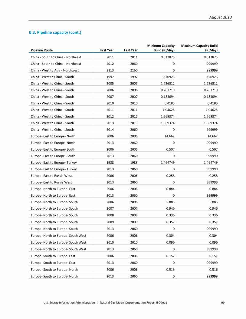
August 2013
U.S. Energy Information Administration | Natural Gas Model Documentation Report IEO2011 99
B.3. Pipeline capacity (cont.)
Pipeline Route First Year Last Year Mininum Capacity
Build (PJ/day) Maxinum Capacity Build
(PJ/day)
China - South to China - Northeast 2011 2011 0.313875 0.313875
China - South to China - Northeast 2012 2060 0 999999
China - West to Asia - Northwest 2113 2160 0 999999
China - West to China - South 1997 1997 0.20925 0.20925
China - West to China - South 2005 2005 1.726312 1.726312
China - West to China - South 2006 2006 0.287719 0.287719
China - West to China - South 2007 2007 0.183094 0.183094
China - West to China - South 2010 2010 0.4185 0.4185
China - West to China - South 2011 2011 1.04625 1.04625
China - West to China - South 2012 2012 1.569374 1.569374
China - West to China - South 2013 2013 1.569374 1.569374
China - West to China - South 2014 2060 0 999999
Europe- East to Europe- North 2006 2006 14.662 14.662
Europe- East to Europe- North 2013 2060 0 999999
Europe- East to Europe- South 2006 2006 0.507 0.507
Europe- East to Europe- South 2013 2060 0 999999
Europe- East to Europe- Turkey 1988 1988 1.464749 1.464749
Europe- East to Europe- Turkey 2013 2060 0 999999
Europe- East to Russia West 2006 2006 0.258 0.258
Europe- East to Russia West 2013 2060 0 999999
Europe- North to Europe- East 2006 2006 0.884 0.884
Europe- North to Europe- East 2013 2060 0 999999
Europe- North to Europe- South 2006 2006 5.885 5.885
Europe- North to Europe- South 2007 2007 0.946 0.946
Europe- North to Europe- South 2008 2008 0.336 0.336
Europe- North to Europe- South 2009 2009 0.357 0.357
Europe- North to Europe- South 2013 2060 0 999999
Europe- North to Europe- South West 2006 2006 0.304 0.304
Europe- North to Europe- South West 2010 2010 0.096 0.096
Europe- North to Europe- South West 2013 2060 0 999999
Europe- South to Europe- East 2006 2006 0.157 0.157
Europe- South to Europe- East 2013 2060 0 999999
Europe- South to Europe- North 2006 2006 0.516 0.516
Europe- South to Europe- North 2013 2060 0 999999

August 2013
U.S. Energy Information Administration | Natural Gas Model Documentation Report IEO2011 100
B.3. Pipeline capacity (cont.)
Pipeline Route First Year Last Year Mininum Capacity
Build (PJ/day) Maxinum Capacity Build
(PJ/day)
Europe- South West to Europe- North 2006 2006 0.0181 0.0181
Europe- South West to Europe- North 2013 2013 0.19115 0.19115
Europe- South West to Europe- North 2015 2015 0.575437 0.575437
Europe- South West to Europe- North 2016 2060 0 999999
Europe- Turkey to Europe- East 2016 2017 0 3.138749
Europe- Turkey to Europe- East 2018 2060 0 999999
Europe- Turkey to Europe- South 2007 2007 0.575437 0.575437
Europe- Turkey to Europe- South 2008 2008 0.575437 0.575437
Europe- Turkey to Europe- South 2013 2060 0 999999
Europe- Turkey to Rest of Middle East 2011 2011 0.104625 0.104625
Europe- Turkey to Rest of Middle East 2013 2060 0 999999
FSU Central Asia to Asia - Northwest 2113 2160 0 999999
FSU Central Asia to China - West 2010 2010 0.523125 0.523125
FSU Central Asia to China - West 2012 2012 3.661873 3.661873
FSU Central Asia to China - West 2013 2060 0 999999
FSU Central Asia to Europe- East 2113 2160 0 999999
FSU Central Asia to Europe- Turkey 2007 2007 0.690525 0.690525
FSU Central Asia to Europe- Turkey 2017 2017 1.401974 1.401974
FSU Central Asia to Europe- Turkey 2018 2060 0 999999
FSU Central Asia to Iran 2006 2006 0.841 0.841
FSU Central Asia to Iran 2010 2010 0.104625 0.104625
FSU Central Asia to Iran 2012 2012 0.523125 0.523125
FSU Central Asia to Iran 2013 2060 0 999999
FSU Central Asia to Russia Caspian Sea 2010 2010 0.523125 0.523125
FSU Central Asia to Russia Caspian Sea 2013 2060 0 999999
FSU Central Asia to Russia West 2005 2005 4.831888 4.831888
FSU Central Asia to Russia West 2006 2006 0 0
FSU Central Asia to Russia West 2013 2060 0 999999
India - Southeast to India - Southwest 2010 2011 0 0.767
India - Southeast to India - Southwest 2012 2013 0 0.767
India - Southeast to India - Southwest 2036 2060 0 999999
India - Southwest to India - North 2006 2006 1.304 1.304
India - Southwest to India - North 2009 2010 0 0.767

August 2013
U.S. Energy Information Administration | Natural Gas Model Documentation Report IEO2011 101
B.3. Pipeline capacity (cont.)
Pipeline Route First Year Last Year
Mininum Capacity Build
(PJ/day) Maxinum Capacity Build
(PJ/day)
India - Southwest to India - North 2011 2012 0 0.767
India - Southwest to India - North 2013 2060 0 999999
Iran to Europe- Turkey 2006 2006 0.62775 0.62775
Iran to Europe- Turkey 2010 2010 0.104625 0.104625
Iran to Europe- Turkey 2011 2011 0.104625 0.104625
Iran to Europe- Turkey 2012 2012 0.20925 0.20925
Iran to Europe- Turkey 2013 2013 0.20925 0.20925
Iran to Europe- Turkey 2014 2014 0.20925 0.20925
Iran to Europe- Turkey 2018 2021 0 1
Iran to Europe- Turkey 2022 2026 0 1
Iran to Europe- Turkey 2027 2030 0 1
Iran to Europe- Turkey 2031 2060 0 999999
Iran to FSU Central Asia 2006 2006 0.076376 0.076376
Iran to FSU Central Asia 2011 2013 0.076376 0.076376
Iran to FSU Central Asia 2014 2160 0 0.087885
Iraq to Arabian Producers 2025 2060 0 0.428962
Iraq to Europe- Turkey 2030 2034 0 0.366831
Iraq to Europe- Turkey 2036 2038 0 0.3154
Iraq to Europe- Turkey 2039 2041 0 0.3154
Iraq to Europe- Turkey 2042 2044 0 0.3154
Iraq to Europe- Turkey 2045 2047 0 0.3154
Iraq to Europe- Turkey 2048 2050 0 0.3154
Iraq to Europe- Turkey 2051 2053 0 0.3154
Iraq to Europe- Turkey 2054 2056 0 0.3154
Iraq to Rest of Middle East 2025 2060 0 0.220099
Latin America - Andean to Brazil 2001 2001 1.148782 1.148782
Latin America - Andean to Brazil 2003 2003 0.09207 0.09207
Latin America - Andean to Brazil 2013 2060 0 999999 Latin America - Andean to Latin America - Southern Cone 2006 2006 0.29295 0.29295 Latin America - Andean to Latin America - Southern Cone 2013 2060 0 999999 Latin America - Central America to US - Florida 2109 2109 0.915 0.915 Latin America - Central America to US - Florida 2113 2160 0 999999

August 2013
U.S. Energy Information Administration | Natural Gas Model Documentation Report IEO2011 102
B.3. Pipeline capacity (cont.)
Pipeline Route First Year Last Year Mininum Capacity
Build (PJ/day) Maxinum Capacity Build
(PJ/day)
Latin America - Northern Producers to Brazil 2113 2160 0 999999 Latin America - Northern Producers to Latin America - Central America 2113 2160 0 999999
Latin America - Southern Cone to Brazil 2001 2001 0.104625 0.104625
Latin America - Southern Cone to Brazil 2013 2060 0 999999
Latin America - Southern Cone to Chile 1996 1996 0.076376 0.076376
Latin America - Southern Cone to Chile 1998 1998 0.363049 0.363049
Latin America - Southern Cone to Chile 1999 1999 0.183094 0.183094
Latin America - Southern Cone to Chile 2000 2000 0.959411 0.959411
Latin America - Southern Cone to Chile 2013 2060 0 999999
Mexico Northeast to US - West South Central 2008 2008 0.935347 0.935347
Mexico Northeast to US - West South Central 2013 2060 0 999999
Mexico Northwest to Mexico Northeast 2013 2060 0 999999
Mexico Northwest to US - AZNM 2013 2060 0 999999
Mexico Northwest to US - California 2008 2008 0.664368 0.664368
Mexico Northwest to US - California 2009 2009 0.087885 0.087885
Mexico Northwest to US - California 2013 2060 0 999999
Mexico South to Mexico Northeast 2006 2006 0.272 0.272
Mexico Southwest LNG to Mexico South 2008 2008 0.815 0.815
Mexico Southwest LNG to Mexico South 2013 2060 0 999999
Qatar to Arabian Producers 2007 2007 2.162598 2.162598
Qatar to Arabian Producers 2015 2060 1.297349 1.297349
Rest of Middle East to Europe- Turkey 2011 2011 0.104625 0.104625
Rest of Middle East to Europe- Turkey 2014 2060 0 999999
Russia Caspian Sea to Europe- Turkey 2006 2006 1.673999 1.673999
Russia Caspian Sea to Europe- Turkey 2015 2030 0 1.63
Russia Caspian Sea to FSU Central Asia 2005 2005 0.20925 0.20925
Russia Caspian Sea to FSU Central Asia 2115 2130 0 999999
Russia Caspian Sea to Russia West 2006 2006 4.184998 4.184998
Russia Caspian Sea to Russia West 2013 2060 0 999999
Russia East to Russia Sakhalin 2023 2060 0 999999
Russia East to Russia West 2013 2060 0 999999
Russia Sakhalin to China - Northeast 2023 2060 0 999999
Russia Sakhalin to Russia East 2006 2006 0.434 0.434
Russia Sakhalin to Russia East 2013 2060 0 999999
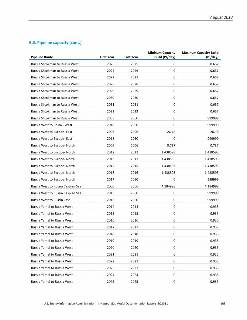
August 2013
U.S. Energy Information Administration | Natural Gas Model Documentation Report IEO2011 103
B.3. Pipeline capacity (cont.)
Pipeline Route First Year Last Year Mininum Capacity
Build (PJ/day) Maxinum Capacity Build
(PJ/day)
Russia Shtokman to Russia West 2025 2025 0 0.657
Russia Shtokman to Russia West 2026 2026 0 0.657
Russia Shtokman to Russia West 2027 2027 0 0.657
Russia Shtokman to Russia West 2028 2028 0 0.657
Russia Shtokman to Russia West 2029 2029 0 0.657
Russia Shtokman to Russia West 2030 2030 0 0.657
Russia Shtokman to Russia West 2031 2031 0 0.657
Russia Shtokman to Russia West 2032 2032 0 0.657
Russia Shtokman to Russia West 2033 2060 0 999999
Russia West to China - West 2018 2060 0 999999
Russia West to Europe- East 2006 2006 26.18 26.18
Russia West to Europe- East 2013 2060 0 999999
Russia West to Europe- North 2006 2006 0.737 0.737
Russia West to Europe- North 2012 2012 1.438593 1.438593
Russia West to Europe- North 2013 2013 1.438593 1.438593
Russia West to Europe- North 2015 2015 1.438593 1.438593
Russia West to Europe- North 2016 2016 1.438593 1.438593
Russia West to Europe- North 2017 2060 0 999999
Russia West to Russia Caspian Sea 2006 2006 4.184998 4.184998
Russia West to Russia Caspian Sea 2013 2060 0 999999
Russia West to Russia East 2013 2060 0 999999
Russia Yamal to Russia West 2014 2014 0 0.935
Russia Yamal to Russia West 2015 2015 0 0.935
Russia Yamal to Russia West 2016 2016 0 0.935
Russia Yamal to Russia West 2017 2017 0 0.935
Russia Yamal to Russia West 2018 2018 0 0.935
Russia Yamal to Russia West 2019 2019 0 0.935
Russia Yamal to Russia West 2020 2020 0 0.935
Russia Yamal to Russia West 2021 2021 0 0.935
Russia Yamal to Russia West 2022 2022 0 0.935
Russia Yamal to Russia West 2023 2023 0 0.935
Russia Yamal to Russia West 2024 2024 0 0.935
Russia Yamal to Russia West 2025 2025 0 0.935

August 2013
U.S. Energy Information Administration | Natural Gas Model Documentation Report IEO2011 104
B.3. Pipeline capacity (cont.)
Pipeline Route First Year Last Year Mininum Capacity
Build (PJ/day) Maxinum Capacity Build
(PJ/day)
Russia Yamal to Russia West 2026 2026 0 0.935
Russia Yamal to Russia West 2027 2027 0 0.935
Russia Yamal to Russia West 2028 2028 0 0.935
Russia Yamal to Russia West 2029 2029 0 0.935
Russia Yamal to Russia West 2030 2030 0 0.935
Russia Yamal to Russia West 2031 2031 0 0.935
Russia Yamal to Russia West 2032 2032 0 0.935
Russia Yamal to Russia West 2033 2033 0 0.935
Russia Yamal to Russia West 2034 2034 0 0.935
Russia Yamal to Russia West 2035 2035 0 0.935
Russia Yamal to Russia West 2036 2060 0 999999
US - Arctic to Canada West 2036 2040 0 4.217
US - Arctic to Canada West 2041 2060 0 999999
US - AZNM to Mexico Northwest 2006 2006 0.284 0.284
US - AZNM to Mexico Northwest 2013 2060 0 999999
US - AZNM to US - California 2008 2008 6.149855 6.149855
US - AZNM to US - California 2013 2060 0 999999
US - AZNM to US - Mountain 2008 2008 0.587992 0.587992
US - AZNM to US - Mountain 2013 2060 0 999999
US - AZNM to US - West South Central 2008 2008 3.613746 3.613746
US - AZNM to US - West South Central 2010 2010 0.107764 0.107764
US - AZNM to US - West South Central 2011 2011 0.037665 0.037665
US - AZNM to US - West South Central 2012 2012 0.899775 1.0044
US - AZNM to US - West South Central 2013 2060 0 999999
US - California to Mexico Northwest 2008 2008 0.892451 0.892451
US - California to Mexico Northwest 2010 2010 0.216574 0.216574
US - California to Mexico Northwest 2013 2060 0 999999
US - California to US - AZNM 2008 2008 0.664368 0.664368
US - California to US - AZNM 2013 2060 0 999999
US - California to US - Mountain 2006 2006 0.176 0.176
US - California to US - Mountain 2013 2060 0 999999
US - East North Central to Canada East 2008 2008 4.277068 4.277068
US - East North Central to Canada East 2011 2011 0.124504 0.124504

August 2013
U.S. Energy Information Administration | Natural Gas Model Documentation Report IEO2011 105
B.3. Pipeline capacity (cont.)
Pipeline Route First Year Last Year
Mininum Capacity Build
(PJ/day) Maxinum Capacity
Build (PJ/day)
US - East North Central to Canada East 2013 2060 0 999999
US - East North Central to US - East South Central 2006 2006 0.618 0.618
US - East North Central to US - East South Central 2013 2060 0 999999
US - East North Central to US - Middle Atlantic 2008 2008 2.316397 2.316397
US - East North Central to US - Middle Atlantic 2010 2010 0.24273 0.24273
US - East North Central to US - Middle Atlantic 2011 2011 0.42687 0.42687
US - East North Central to US - Middle Atlantic 2013 2060 0 999999
US - East North Central to US - South Atlantic 2008 2008 3.140841 3.140841
US - East North Central to US - South Atlantic 2013 2060 0 999999
US - East North Central to US - West North Central 2008 2008 1.043111 1.043111
US - East North Central to US - West North Central 2013 2060 0 999999
US - East South Central to US - East North Central 2008 2008 10.02098 10.02098
US - East South Central to US - East North Central 2013 2060 0 999999
US - East South Central to US - Florida 2008 2008 3.999812 3.999812
US - East South Central to US - Florida 2011 2011 0.810843 0.810843
US - East South Central to US - Florida 2013 2060 0 999999
US - East South Central to US - South Atlantic 2008 2008 11.13733 11.13733
US - East South Central to US - South Atlantic 2011 2011 0.236452 0.236452
US - East South Central to US - South Atlantic 2012 2012 0.134966 0.134966
US - East South Central to US - South Atlantic 2013 2060 0 999999
US - East South Central to US - West South Central 2008 2008 0.438379 0.438379
US - East South Central to US - West South Central 2013 2060 0 999999
US - Middle Atlantic to Canada East 2008 2008 0.107764 0.107764
US - Middle Atlantic to Canada East 2012 2012 0.189371 0.189371
US - Middle Atlantic to Canada East 2013 2060 0 999999
US - Middle Atlantic to US - East North Central 2006 2006 0.505 0.505
US - Middle Atlantic to US - East North Central 2013 2060 0 999999
US - Middle Atlantic to US - New England 2008 2008 3.828227 3.828227
US - Middle Atlantic to US - New England 2013 2060 0 999999
US - Middle Atlantic to US - South Atlantic 2008 2008 3.045632 3.045632
US - Middle Atlantic to US - South Atlantic 2013 2060 0 999999
US - Mountain to Canada West 2006 2006 0.081 0.081

August 2013
U.S. Energy Information Administration | Natural Gas Model Documentation Report IEO2011 106
B.3. Pipeline capacity (cont.)
Pipeline Route First Year Last Year
Mininum Capacity Build (PJ/day)
Maxinum Capacity Build (PJ/day)
US - Mountain to Canada West 2013 2060 0 999999
US - Mountain to US - AZNM 2008 2008 2.376033 2.376033
US - Mountain to US - AZNM 2013 2060 0 999999
US - Mountain to US - California 2008 2008 1.923007 1.923007
US - Mountain to US - California 2010 2010 0.156937 0.156937
US - Mountain to US - California 2013 2060 0 999999
US - Mountain to US - Pacific Northwest 2008 2008 3.615839 3.615839
US - Mountain to US - Pacific Northwest 2013 2060 0 999999
US - Mountain to US - West North Central 2008 2008 10.74289 10.74289
US - Mountain to US - West North Central 2009 2009 0.081607 0.081607
US - Mountain to US - West North Central 2010 2010 0.515801 0.515801
US - Mountain to US - West North Central 2013 2060 0 999999
US - Mountain to US - West South Central 2006 2006 0.527 0.527
US - Mountain to US - West South Central 2013 2060 0 999999
US - New England to Canada East 2008 2008 0.233314 0.233314
US - New England to Canada East 2013 2060 0 999999
US - New England to US - Middle Atlantic 2008 2008 0.561836 0.561836
US - New England to US - Middle Atlantic 2013 2060 0 999999
US - Pacific Northwest to Canada West 2006 2006 0.055 0.055
US - Pacific Northwest to Canada West 2013 2060 0 999999
US - Pacific Northwest to US - California 2008 2008 2.585283 2.585283
US - Pacific Northwest to US - California 2013 2060 0 999999
US - Pacific Northwest to US - Mountain 2006 2006 0.065 0.065
US - Pacific Northwest to US - Mountain 2013 2060 0 999999
US - South Atlantic to US - East North Central 2006 2006 1.766 1.766
US - South Atlantic to US - East North Central 2013 2060 0 999999
US - South Atlantic to US - East South Central 2006 2006 0.23 0.23
US - South Atlantic to US - East South Central 2013 2060 0 999999
US - South Atlantic to US - Florida 2008 2008 0.444656 0.444656
US - South Atlantic to US - Florida 2013 2060 0 999999
US - South Atlantic to US - Middle Atlantic 2008 2008 9.334639 9.334639
US - South Atlantic to US - Middle Atlantic 2009 2009 0.162169 0.162169
US - South Atlantic to US - Middle Atlantic 2010 2010 0.107764 0.107764

August 2013
U.S. Energy Information Administration | Natural Gas Model Documentation Report IEO2011 107
B.3. Pipeline capacity (cont.)
Pipeline Route First Year Last Year Mininum Capacity
Build (PJ/day) Maxinum Capacity
Build (PJ/day)
US - South Atlantic to US - Middle Atlantic 2011 2011 0.648675 0.648675
US - South Atlantic to US - Middle Atlantic 2012 2012 0.524171 0.524171
US - South Atlantic to US - Middle Atlantic 2013 2060 0 999999
US - West North Central to Canada East 2008 2008 0.068006 0.068006
US - West North Central to Canada East 2013 2060 0 999999 US - West North Central to US - East North Central 2008 2008 13.95592 13.95592 US - West North Central to US - East North Central 2009 2009 1.730497 1.730497 US - West North Central to US - East North Central 2013 2060 0 999999
US - West North Central to US - Mountain 2008 2008 3.82195 3.82195
US - West North Central to US - Mountain 2013 2060 0 999999 US - West North Central to US - West South Central 2008 2008 0.986613 0.986613 US - West North Central to US - West South Central 2013 2060 0 999999
US - West South Central to Mexico Northeast 2008 2008 2.757914 2.757914
US - West South Central to Mexico Northeast 2013 2060 0 999999
US - West South Central to US - AZNM 2008 2008 5.014674 5.014674
US - West South Central to US - AZNM 2013 2060 0 999999 US - West South Central to US - East South Central 2008 2008 27.06962 27.06962 US - West South Central to US - East South Central 2009 2009 2.703509 2.703509 US - West South Central to US - East South Central 2010 2010 1.621687 1.621687 US - West South Central to US - East South Central 2011 2011 2.551803 2.551803 US - West South Central to US - East South Central 2012 2012 2.811273 2.811273 US - West South Central to US - East South Central 2013 2060 0 999999
US - West South Central to US - Mountain 2008 2008 0.216574 0.216574
US - West South Central to US - Mountain 2013 2060 0 999999 US - West South Central to US - West North Central 2008 2008 9.135851 9.135851 US - West South Central to US - West North Central 2011 2011 0.216574 0.216574 US - West South Central to US - West North Central 2013 2060 0 999999
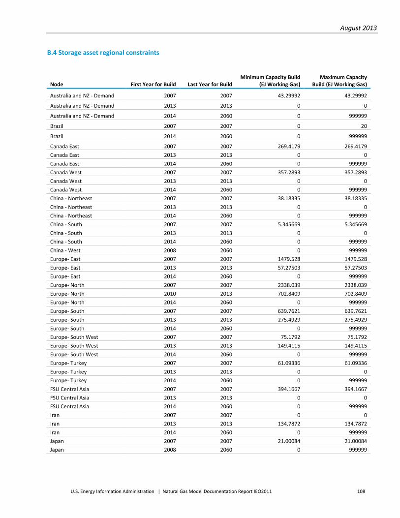
August 2013
U.S. Energy Information Administration | Natural Gas Model Documentation Report IEO2011 108
B.4 Storage asset regional constraints
Node First Year for Build Last Year for Build Minimum Capacity Build
(EJ Working Gas) Maximum Capacity
Build (EJ Working Gas)
Australia and NZ - Demand 2007 2007 43.29992 43.29992
Australia and NZ - Demand 2013 2013 0 0
Australia and NZ - Demand 2014 2060 0 999999
Brazil 2007 2007 0 20
Brazil 2014 2060 0 999999
Canada East 2007 2007 269.4179 269.4179 Canada East 2013 2013 0 0 Canada East 2014 2060 0 999999 Canada West 2007 2007 357.2893 357.2893 Canada West 2013 2013 0 0 Canada West 2014 2060 0 999999 China - Northeast 2007 2007 38.18335 38.18335 China - Northeast 2013 2013 0 0 China - Northeast 2014 2060 0 999999 China - South 2007 2007 5.345669 5.345669 China - South 2013 2013 0 0 China - South 2014 2060 0 999999 China - West 2008 2060 0 999999 Europe- East 2007 2007 1479.528 1479.528 Europe- East 2013 2013 57.27503 57.27503 Europe- East 2014 2060 0 999999 Europe- North 2007 2007 2338.039 2338.039 Europe- North 2010 2013 702.8409 702.8409 Europe- North 2014 2060 0 999999 Europe- South 2007 2007 639.7621 639.7621 Europe- South 2013 2013 275.4929 275.4929 Europe- South 2014 2060 0 999999 Europe- South West 2007 2007 75.1792 75.1792 Europe- South West 2013 2013 149.4115 149.4115 Europe- South West 2014 2060 0 999999 Europe- Turkey 2007 2007 61.09336 61.09336 Europe- Turkey 2013 2013 0 0 Europe- Turkey 2014 2060 0 999999 FSU Central Asia 2007 2007 394.1667 394.1667 FSU Central Asia 2013 2013 0 0 FSU Central Asia 2014 2060 0 999999 Iran 2007 2007 0 0 Iran 2013 2013 134.7872 134.7872 Iran 2014 2060 0 999999 Japan 2007 2007 21.00084 21.00084 Japan 2008 2060 0 999999

August 2013
U.S. Energy Information Administration | Natural Gas Model Documentation Report IEO2011 109
B.4 Storage asset regional constraints (cont.)
Node First Year for Build Last Year for Build Minimum Capacity Build
(EJ Working Gas) Maximum Capacity
Build (EJ Working Gas) Latin America - Southern Cone 2007 2007 3.818335 3.818335 Latin America - Southern Cone 2013 2013 0 0 Latin America - Southern Cone 2014 2060 0 999999 Russia Caspian Sea 2007 2007 1147.41 1147.41 Russia Caspian Sea 2013 2013 0 0 Russia Caspian Sea 2014 2060 0 999999 Russia East 2007 2007 116.2683 116.2683 Russia East 2013 2013 0 0 Russia East 2014 2060 0 999999 Russia West 2007 2007 1239.661 1239.661 Russia West 2013 2013 0 0 Russia West 2014 2060 0 999999 US - AZNM 2007 2007 51.39097 51.39097 US - AZNM 2013 2013 0 0 US - AZNM 2014 2060 0 999999 US - California 2007 2007 264.729 264.729 US - California 2013 2013 0 0 US - California 2014 2060 0 999999 US - East North Central 2007 2007 1248.179 1248.179 US - East North Central 2013 2013 0 0 US - East North Central 2014 2060 0 999999 US - East South Central 2007 2007 182.673 182.673 US - East South Central 2013 2013 0 0 US - East South Central 2014 2060 0 999999 US - Middle Atlantic 2007 2007 548.5458 548.5458 US - Middle Atlantic 2013 2013 0 0 US - Middle Atlantic 2014 2060 0 999999 US - Mountain 2007 2007 355.7734 355.7734 US - Mountain 2013 2013 0 0 US - Mountain 2014 2060 0 999999 US - Pacific Northwest 2007 2007 43.76194 43.76194 US - Pacific Northwest 2013 2013 0 0 US - Pacific Northwest 2014 2060 0 999999 US - South Atlantic 2007 2007 256.9625 256.9625 US - South Atlantic 2013 2013 0 0 US - South Atlantic 2014 2060 0 999999 US - West North Central 2007 2007 206.9156 206.9156 US - West North Central 2013 2013 0 0 US - West North Central 2014 2060 0 999999

August 2013
U.S. Energy Information Administration | Natural Gas Model Documentation Report IEO2011 110
B.5 Resource availability constraints
Node Supply Catagory Year
Share of Resource that is available for
development
Africa - North Conventional Onshore 2008 1
Africa - North Conventional Offshore 2008 1
Africa - North Tight Gas 2008 0
Africa - North Tight Gas 2010 0
Africa - North Tight Gas 2012 1
Africa - North Tight Gas 2020 1
Africa - North CoalBed Methane 2008 0
Africa - North CoalBed Methane 2018 0
Africa - North CoalBed Methane 2023 0.3
Africa - North CoalBed Methane 2028 1
Africa - North Shale Gas 2008 0
Africa - North Shale Gas 2013 0
Africa - North Shale Gas 2018 0.2
Africa - North Shale Gas 2028 1
Africa - Rest Conventional Onshore 2008 1
Africa - Rest Conventional Offshore 2008 1
Africa - Rest Tight Gas 2008 0
Africa - Rest Tight Gas 2020 0
Africa - Rest Tight Gas 2025 0.3
Africa - Rest Tight Gas 2030 1
Africa - Rest CoalBed Methane 2008 0
Africa - Rest CoalBed Methane 2013 0
Africa - Rest CoalBed Methane 2018 0.3
Africa - Rest CoalBed Methane 2023 1
Africa - Rest Shale Gas 2008 0
Africa - Rest Shale Gas 2023 0
Africa - Rest Shale Gas 2028 0.2
Africa - Rest Shale Gas 2038 1
Africa - South Conventional Onshore 2008 1
Africa - South Conventional Offshore 2008 1
Africa - South Tight Gas 2008 0
Africa - South Tight Gas 2015 0
Africa - South Tight Gas 2020 0.3
Africa - South Tight Gas 2025 1

August 2013
U.S. Energy Information Administration | Natural Gas Model Documentation Report IEO2011 111
B.5 Resource availability constraints (cont.)
Node Supply Catagory Year
Share of Resource that is available for
development
Africa - South CoalBed Methane 2008 0
Africa - South CoalBed Methane 2013 0
Africa - South CoalBed Methane 2018 0.3
Africa - South CoalBed Methane 2023 1
Africa - South Shale Gas 2008 0
Africa - South Shale Gas 2018 0
Africa - South Shale Gas 2023 0.2
Africa - South Shale Gas 2033 1
Africa - West Conventional Onshore 2008 1
Africa - West Conventional Offshore 2008 1
Africa - West Tight Gas 2008 0
Africa - West Tight Gas 2020 0
Africa - West Tight Gas 2025 0.3
Africa - West Tight Gas 2030 1
Africa - West CoalBed Methane 2008 0
Africa - West CoalBed Methane 2018 0
Africa - West CoalBed Methane 2023 0.3
Africa - West CoalBed Methane 2028 1
Africa - West Shale Gas 2008 0
Africa - West Shale Gas 2023 0
Africa - West Shale Gas 2028 0.2
Africa - West Shale Gas 2038 1
Asia - Northwest Conventional Onshore 2008 1
Asia - Northwest Conventional Offshore 2008 1
Asia - Northwest Tight Gas 2008 0
Asia - Northwest Tight Gas 2015 0
Asia - Northwest Tight Gas 2020 0.3
Asia - Northwest Tight Gas 2025 1
Asia - Northwest CoalBed Methane 2008 0
Asia - Northwest CoalBed Methane 2018 0
Asia - Northwest CoalBed Methane 2023 0.3
Asia - Northwest CoalBed Methane 2028 1
Asia - Northwest Shale Gas 2008 0
Asia - Northwest Shale Gas 2018 0

August 2013
U.S. Energy Information Administration | Natural Gas Model Documentation Report IEO2011 112
B.5 Resource availability constraints (cont.)
Node Supply Catagory Year
Share of Resource that is available for
development
Asia - Northwest Shale Gas 2023 0.2
Asia - Northwest Shale Gas 2033 1
Asia - Other Developed Conventional Onshore 2008 1
Asia - Other Developed Conventional Offshore 2008 1
Asia - Other Developed Tight Gas 2008 0
Asia - Other Developed Tight Gas 2020 0
Asia - Other Developed Tight Gas 2025 0.3
Asia - Other Developed Tight Gas 2030 1
Asia - Other Developed CoalBed Methane 2008 0
Asia - Other Developed CoalBed Methane 2018 0
Asia - Other Developed CoalBed Methane 2023 0.3
Asia - Other Developed CoalBed Methane 2028 1
Asia - Other Developed Shale Gas 2008 0
Asia - Other Developed Shale Gas 2023 0
Asia - Other Developed Shale Gas 2028 0.2
Asia - Other Developed Shale Gas 2038 1
Asia - Other Developing SE Conventional Onshore 2008 1
Asia - Other Developing SE Conventional Offshore 2008 1
Asia - Other Developing SE Tight Gas 2008 0
Asia - Other Developing SE Tight Gas 2020 0
Asia - Other Developing SE Tight Gas 2025 0.3
Asia - Other Developing SE Tight Gas 2030 1
Asia - Other Developing SE CoalBed Methane 2008 0
Asia - Other Developing SE CoalBed Methane 2018 0
Asia - Other Developing SE CoalBed Methane 2023 0.3
Asia - Other Developing SE CoalBed Methane 2028 1
Asia - Other Developing SE Shale Gas 2008 0
Asia - Other Developing SE Shale Gas 2023 0
Asia - Other Developing SE Shale Gas 2028 0.2
Asia - Other Developing SE Shale Gas 2038 1
Asia - Producers Conventional Onshore 2008 1
Asia - Producers Conventional Offshore 2008 1
Asia - Producers Tight Gas 2008 0
Asia - Producers Tight Gas 2020 0

August 2013
U.S. Energy Information Administration | Natural Gas Model Documentation Report IEO2011 113
B.5 Resource availability constraints (cont.)
Node Supply Catagory Year
Share of Resource that is available for
development
Asia - Producers Tight Gas 2025 0.3
Asia - Producers Tight Gas 2030 1
Asia - Producers CoalBed Methane 2008 0
Asia - Producers CoalBed Methane 2013 0.5
Asia - Producers CoalBed Methane 2015 1
Asia - Producers Shale Gas 2008 0
Asia - Producers Shale Gas 2018 0
Asia - Producers Shale Gas 2023 0.2
Asia - Producers Shale Gas 2033 1
Australia and NZ - Demand Conventional Onshore 2008 1
Australia and NZ - Demand Conventional Offshore 2008 1
Australia and NZ - Demand Tight Gas 2008 0
Australia and NZ - Demand Tight Gas 2010 0
Australia and NZ - Demand Tight Gas 2015 0.3
Australia and NZ - Demand Tight Gas 2020 1
Australia and NZ - Demand CoalBed Methane 2008 0.5
Australia and NZ - Demand CoalBed Methane 2014 1
Australia and NZ - Demand Shale Gas 2008 0
Australia and NZ - Demand Shale Gas 2013 0
Australia and NZ - Demand Shale Gas 2018 0.2
Australia and NZ - Demand Shale Gas 2028 1
Australia and NZ - NW Shelf Conventional Onshore 2008 1
Australia and NZ - NW Shelf Conventional Offshore 2008 1
Australia and NZ - NW Shelf Tight Gas 2008 0
Australia and NZ - NW Shelf Tight Gas 2015 0
Australia and NZ - NW Shelf Tight Gas 2020 0.3
Australia and NZ - NW Shelf Tight Gas 2025 1
Australia and NZ - NW Shelf CoalBed Methane 2008 0
Australia and NZ - NW Shelf CoalBed Methane 2018 0
Australia and NZ - NW Shelf CoalBed Methane 2023 0.3
Australia and NZ - NW Shelf CoalBed Methane 2028 1
Australia and NZ - NW Shelf Shale Gas 2008 0
Australia and NZ - NW Shelf Shale Gas 2018 0
Australia and NZ - NW Shelf Shale Gas 2023 0.2

August 2013
U.S. Energy Information Administration | Natural Gas Model Documentation Report IEO2011 114
B.5 Resource availability constraints (cont.)
Node Supply Catagory Year
Share of Resource that is available for
development
Australia and NZ - NW Shelf Shale Gas 2033 1
Brazil Conventional Onshore 2008 1
Brazil Conventional Offshore 2008 1
Brazil Tight Gas 2008 0
Brazil Tight Gas 2015 0
Brazil Tight Gas 2020 0.3
Brazil Tight Gas 2025 1
Brazil CoalBed Methane 2008 0
Brazil CoalBed Methane 2013 0
Brazil CoalBed Methane 2018 0.3
Brazil CoalBed Methane 2023 1
Brazil Shale Gas 2008 0
Brazil Shale Gas 2023 0
Brazil Shale Gas 2028 0.2
Brazil Shale Gas 2038 1
Canada East Conventional Onshore 2008 1
Canada East Conventional Offshore 2008 1
Canada East Tight Gas 2008 1
Canada East CoalBed Methane 2008 0.5
Canada East CoalBed Methane 2014 0.5
Canada East CoalBed Methane 2024 1
Canada East Shale Gas 2008 0
Canada East Shale Gas 2012 1
Canada West Conventional Onshore 2008 1
Canada West Conventional Offshore 2008 1
Canada West Tight Gas 2008 1
Canada West CoalBed Methane 2008 0.5
Canada West CoalBed Methane 2014 0.5
Canada West CoalBed Methane 2024 1
Canada West Shale Gas 2008 0
Canada West Shale Gas 2012 1
Chile Conventional Onshore 2008 1
Chile Conventional Offshore 2008 1
Chile Tight Gas 2008 0

August 2013
U.S. Energy Information Administration | Natural Gas Model Documentation Report IEO2011 115
B.5 Resource availability constraints (cont.)
Node Supply Catagory Year
Share of Resource that is available for
development
Chile Tight Gas 2015 0
Chile Tight Gas 2020 0.3
Chile Tight Gas 2025 1
Chile CoalBed Methane 2008 0
Chile CoalBed Methane 2018 0
Chile CoalBed Methane 2023 0.3
Chile CoalBed Methane 2028 1
Chile Shale Gas 2008 0
Chile Shale Gas 2018 0
Chile Shale Gas 2023 0.2
Chile Shale Gas 2033 1
China - Northeast Conventional Onshore 2008 1
China - Northeast Conventional Offshore 2008 1
China - Northeast Tight Gas 2008 1
China - Northeast CoalBed Methane 2008 0
China - Northeast CoalBed Methane 2013 0.5
China - Northeast CoalBed Methane 2018 1
China - Northeast Shale Gas 2008 0
China - Northeast Shale Gas 2018 0
China - Northeast Shale Gas 2023 0.2
China - Northeast Shale Gas 2033 1
China - South Conventional Onshore 2008 1
China - South Conventional Offshore 2008 1
China - South Tight Gas 2008 1
China - South CoalBed Methane 2008 0
China - South CoalBed Methane 2013 0.5
China - South CoalBed Methane 2018 1
China - South Shale Gas 2008 0
China - South Shale Gas 2018 0
China - South Shale Gas 2023 0.2
China - South Shale Gas 2033 1
China - West Conventional Onshore 2008 1
China - West Conventional Offshore 2008 1
China - West Tight Gas 2008 1
China - West CoalBed Methane 2008 0

August 2013
U.S. Energy Information Administration | Natural Gas Model Documentation Report IEO2011 116
B.5 Resource availability constraints (cont.)
Node Supply Catagory Year
Share of Resource that is available for
development
China - West CoalBed Methane 2013 0.5
China - West CoalBed Methane 2018 1
China - West Shale Gas 2008 0
China - West Shale Gas 2013 0
China - West Shale Gas 2018 0.2
China - West Shale Gas 2028 1
Europe- East Conventional Onshore 2008 1
Europe- East Conventional Offshore 2008 1
Europe- East Tight Gas 2008 0
Europe- East Tight Gas 2015 0
Europe- East Tight Gas 2020 0.3
Europe- East Tight Gas 2025 1
Europe- East CoalBed Methane 2008 0
Europe- East CoalBed Methane 2013 0
Europe- East CoalBed Methane 2018 0.3
Europe- East CoalBed Methane 2023 1
Europe- East Shale Gas 2008 0
Europe- East Shale Gas 2018 0
Europe- East Shale Gas 2030 0.2
Europe- East Shale Gas 2040 1
Europe- North Conventional Onshore 2008 1
Europe- North Conventional Offshore 2008 1
Europe- North Tight Gas 2008 0
Europe- North Tight Gas 2015 0
Europe- North Tight Gas 2020 0.3
Europe- North Tight Gas 2025 1
Europe- North CoalBed Methane 2008 0
Europe- North CoalBed Methane 2013 0.3
Europe- North CoalBed Methane 2018 1
Europe- North Shale Gas 2008 0
Europe- North Shale Gas 2013 0
Europe- North Shale Gas 2018 0.2
Europe- North Shale Gas 2028 1
Europe- South Conventional Onshore 2008 1

August 2013
U.S. Energy Information Administration | Natural Gas Model Documentation Report IEO2011 117
B.5 Resource availability constraints (cont.)
Node Supply Catagory Year
Share of Resource that is available for
development
Europe- South Conventional Offshore 2008 1
Europe- South Tight Gas 2008 0
Europe- South Tight Gas 2015 0
Europe- South Tight Gas 2020 0.3
Europe- South Tight Gas 2025 1
Europe- South CoalBed Methane 2008 0
Europe- South CoalBed Methane 2013 0
Europe- South CoalBed Methane 2018 0.3
Europe- South CoalBed Methane 2023 1
Europe- South Shale Gas 2008 0
Europe- South Shale Gas 2018 0
Europe- South Shale Gas 2023 0.2
Europe- South Shale Gas 2033 1
Europe- South West Conventional Onshore 2008 1
Europe- South West Conventional Offshore 2008 1
Europe- South West Tight Gas 2008 0
Europe- South West Tight Gas 2015 0
Europe- South West Tight Gas 2020 0.3
Europe- South West Tight Gas 2025 1
Europe- South West CoalBed Methane 2008 0
Europe- South West CoalBed Methane 2018 0
Europe- South West CoalBed Methane 2023 0.3
Europe- South West CoalBed Methane 2028 1
Europe- South West Shale Gas 2008 0
Europe- South West Shale Gas 2018 0
Europe- South West Shale Gas 2023 0.2
Europe- South West Shale Gas 2033 1
Europe- Turkey Conventional Onshore 2008 1
Europe- Turkey Conventional Offshore 2008 1
Europe- Turkey Tight Gas 2008 0
Europe- Turkey Tight Gas 2015 0
Europe- Turkey Tight Gas 2020 0.3
Europe- Turkey Tight Gas 2025 1
Europe- Turkey CoalBed Methane 2008 0

August 2013
U.S. Energy Information Administration | Natural Gas Model Documentation Report IEO2011 118
B.5 Resource availability constraints (cont.)
Node Supply Catagory Year
Share of Resource that is available for
development
Europe- Turkey CoalBed Methane 2018 0
Europe- Turkey CoalBed Methane 2023 0.3
Europe- Turkey CoalBed Methane 2028 1
Europe- Turkey Shale Gas 2008 0
Europe- Turkey Shale Gas 2018 0
Europe- Turkey Shale Gas 2023 0.2
Europe- Turkey Shale Gas 2033 1
FSU Central Asia Conventional Onshore 2008 1
FSU Central Asia Conventional Offshore 2008 1
FSU Central Asia Tight Gas 2008 0
FSU Central Asia Tight Gas 2020 0
FSU Central Asia Tight Gas 2025 0.3
FSU Central Asia Tight Gas 2030 1
FSU Central Asia CoalBed Methane 2008 0
FSU Central Asia CoalBed Methane 2018 0
FSU Central Asia CoalBed Methane 2023 0.3
FSU Central Asia CoalBed Methane 2028 1
FSU Central Asia Shale Gas 2008 0
FSU Central Asia Shale Gas 2023 0
FSU Central Asia Shale Gas 2028 0.2
FSU Central Asia Shale Gas 2038 1
India - North Conventional Onshore 2008 1
India - North Conventional Offshore 2008 1
India - North Tight Gas 2008 0
India - North Tight Gas 2020 0
India - North Tight Gas 2025 0.3
India - North Tight Gas 2030 1
India - North CoalBed Methane 2008 0
India - North CoalBed Methane 2013 0.3
India - North CoalBed Methane 2018 1
India - North Shale Gas 2008 0
India - North Shale Gas 2018 0
India - North Shale Gas 2023 0.2
India - North Shale Gas 2033 1
India - Southeast Conventional Onshore 2008 1

August 2013
U.S. Energy Information Administration | Natural Gas Model Documentation Report IEO2011 119
B.5 Resource availability constraints (cont.)
Node Supply Catagory Year
Share of Resource that is available for
development
India - Southeast Conventional Offshore 2008 1
India - Southeast Tight Gas 2008 0
India - Southeast Tight Gas 2020 0
India - Southeast Tight Gas 2025 0.3
India - Southeast Tight Gas 2030 1
India - Southeast CoalBed Methane 2008 0
India - Southeast CoalBed Methane 2013 0.3
India - Southeast CoalBed Methane 2018 1
India - Southeast Shale Gas 2008 0
India - Southeast Shale Gas 2018 0
India - Southeast Shale Gas 2023 0.2
India - Southeast Shale Gas 2033 1
India - Southwest Conventional Onshore 2008 1
India - Southwest Conventional Offshore 2008 1
India - Southwest Tight Gas 2008 0
India - Southwest Tight Gas 2020 0
India - Southwest Tight Gas 2025 0.3
India - Southwest Tight Gas 2030 1
India - Southwest CoalBed Methane 2008 0
India - Southwest CoalBed Methane 2013 0.3
India - Southwest CoalBed Methane 2018 1
India - Southwest Shale Gas 2008 0
India - Southwest Shale Gas 2018 0
India - Southwest Shale Gas 2023 0.2
India - Southwest Shale Gas 2033 1
Japan Conventional Onshore 2008 1
Japan Conventional Offshore 2008 1
Japan Tight Gas 2008 0
Japan Tight Gas 2020 0
Japan Tight Gas 2025 0.3
Japan Tight Gas 2030 1
Japan CoalBed Methane 2008 0
Japan CoalBed Methane 2018 0
Japan CoalBed Methane 2023 0.3
Japan CoalBed Methane 2028 1

August 2013
U.S. Energy Information Administration | Natural Gas Model Documentation Report IEO2011 120
B.5 Resource availability constraints (cont.)
Node Supply Catagory Year
Share of Resource that is available for
development
Japan Shale Gas 2008 0
Japan Shale Gas 2023 0
Japan Shale Gas 2028 0.2
Japan Shale Gas 2038 1
Latin America - Andean Conventional Onshore 2008 1
Latin America - Andean Conventional Offshore 2008 1
Latin America - Andean Tight Gas 2008 0
Latin America - Andean Tight Gas 2020 0
Latin America - Andean Tight Gas 2025 0.3
Latin America - Andean Tight Gas 2030 1
Latin America - Andean CoalBed Methane 2008 0
Latin America - Andean CoalBed Methane 2018 0
Latin America - Andean CoalBed Methane 2023 0.3
Latin America - Andean CoalBed Methane 2028 1
Latin America - Andean Shale Gas 2008 0
Latin America - Andean Shale Gas 2018 0
Latin America - Andean Shale Gas 2023 0.2
Latin America - Andean Shale Gas 2033 1
Latin America - Central America Conventional Onshore 2008 1
Latin America - Central America Conventional Offshore 2008 1
Latin America - Central America Tight Gas 2008 0
Latin America - Central America Tight Gas 2020 0
Latin America - Central America Tight Gas 2025 0.3
Latin America - Central America Tight Gas 2030 1
Latin America - Central America CoalBed Methane 2008 0
Latin America - Central America CoalBed Methane 2018 0
Latin America - Central America CoalBed Methane 2023 0.3
Latin America - Central America CoalBed Methane 2028 1
Latin America - Central America Shale Gas 2008 0
Latin America - Central America Shale Gas 2023 0
Latin America - Central America Shale Gas 2028 0.2
Latin America - Central America Shale Gas 2038 1
Latin America - Northern Producers Conventional Onshore 2008 1
Latin America - Northern Producers Conventional Offshore 2008 1
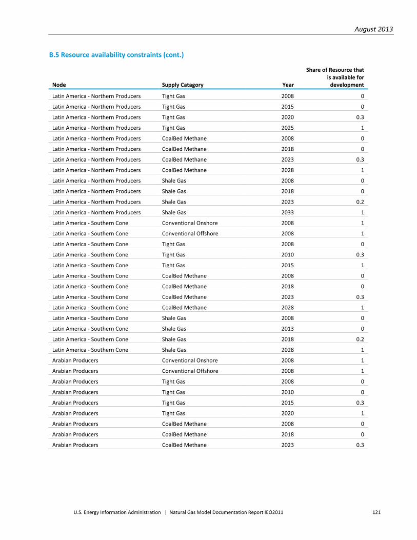
August 2013
U.S. Energy Information Administration | Natural Gas Model Documentation Report IEO2011 121
B.5 Resource availability constraints (cont.)
Node Supply Catagory Year
Share of Resource that is available for
development
Latin America - Northern Producers Tight Gas 2008 0
Latin America - Northern Producers Tight Gas 2015 0
Latin America - Northern Producers Tight Gas 2020 0.3
Latin America - Northern Producers Tight Gas 2025 1
Latin America - Northern Producers CoalBed Methane 2008 0
Latin America - Northern Producers CoalBed Methane 2018 0
Latin America - Northern Producers CoalBed Methane 2023 0.3
Latin America - Northern Producers CoalBed Methane 2028 1
Latin America - Northern Producers Shale Gas 2008 0
Latin America - Northern Producers Shale Gas 2018 0
Latin America - Northern Producers Shale Gas 2023 0.2
Latin America - Northern Producers Shale Gas 2033 1
Latin America - Southern Cone Conventional Onshore 2008 1
Latin America - Southern Cone Conventional Offshore 2008 1
Latin America - Southern Cone Tight Gas 2008 0
Latin America - Southern Cone Tight Gas 2010 0.3
Latin America - Southern Cone Tight Gas 2015 1
Latin America - Southern Cone CoalBed Methane 2008 0
Latin America - Southern Cone CoalBed Methane 2018 0
Latin America - Southern Cone CoalBed Methane 2023 0.3
Latin America - Southern Cone CoalBed Methane 2028 1
Latin America - Southern Cone Shale Gas 2008 0
Latin America - Southern Cone Shale Gas 2013 0
Latin America - Southern Cone Shale Gas 2018 0.2
Latin America - Southern Cone Shale Gas 2028 1
Arabian Producers Conventional Onshore 2008 1
Arabian Producers Conventional Offshore 2008 1
Arabian Producers Tight Gas 2008 0
Arabian Producers Tight Gas 2010 0
Arabian Producers Tight Gas 2015 0.3
Arabian Producers Tight Gas 2020 1
Arabian Producers CoalBed Methane 2008 0
Arabian Producers CoalBed Methane 2018 0
Arabian Producers CoalBed Methane 2023 0.3
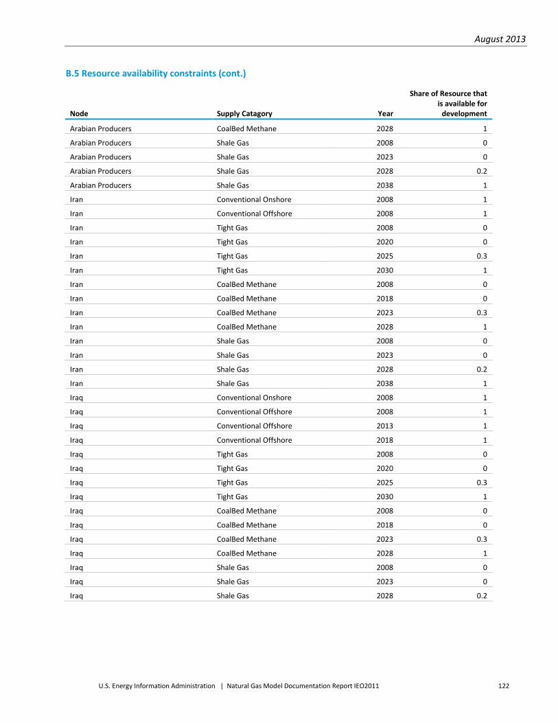
August 2013
U.S. Energy Information Administration | Natural Gas Model Documentation Report IEO2011 122
B.5 Resource availability constraints (cont.)
Node Supply Catagory Year
Share of Resource that is available for
development
Arabian Producers CoalBed Methane 2028 1
Arabian Producers Shale Gas 2008 0
Arabian Producers Shale Gas 2023 0
Arabian Producers Shale Gas 2028 0.2
Arabian Producers Shale Gas 2038 1
Iran Conventional Onshore 2008 1
Iran Conventional Offshore 2008 1
Iran Tight Gas 2008 0
Iran Tight Gas 2020 0
Iran Tight Gas 2025 0.3
Iran Tight Gas 2030 1
Iran CoalBed Methane 2008 0
Iran CoalBed Methane 2018 0
Iran CoalBed Methane 2023 0.3
Iran CoalBed Methane 2028 1
Iran Shale Gas 2008 0
Iran Shale Gas 2023 0
Iran Shale Gas 2028 0.2
Iran Shale Gas 2038 1
Iraq Conventional Onshore 2008 1
Iraq Conventional Offshore 2008 1
Iraq Conventional Offshore 2013 1
Iraq Conventional Offshore 2018 1
Iraq Tight Gas 2008 0
Iraq Tight Gas 2020 0
Iraq Tight Gas 2025 0.3
Iraq Tight Gas 2030 1
Iraq CoalBed Methane 2008 0
Iraq CoalBed Methane 2018 0
Iraq CoalBed Methane 2023 0.3
Iraq CoalBed Methane 2028 1
Iraq Shale Gas 2008 0
Iraq Shale Gas 2023 0
Iraq Shale Gas 2028 0.2

August 2013
U.S. Energy Information Administration | Natural Gas Model Documentation Report IEO2011 123
B.5 Resource availability constraints (cont.)
Node Supply Catagory Year
Share of Resource that is available for
development
Iraq Shale Gas 2038 1
Qatar Conventional Onshore 2008 1
Qatar Conventional Offshore 2008 1
Qatar Tight Gas 2008 0
Qatar Tight Gas 2020 0
Qatar Tight Gas 2025 0.3
Qatar Tight Gas 2030 1
Qatar CoalBed Methane 2008 0
Qatar CoalBed Methane 2018 0
Qatar CoalBed Methane 2023 0.3
Qatar CoalBed Methane 2028 1
Qatar Shale Gas 2008 0
Qatar Shale Gas 2023 0
Qatar Shale Gas 2028 0.2
Qatar Shale Gas 2038 1
Rest of Middle East Conventional Onshore 2008 1
Rest of Middle East Conventional Offshore 2008 1
Rest of Middle East Tight Gas 2008 0
Rest of Middle East Tight Gas 2015 0
Rest of Middle East Tight Gas 2020 0.3
Rest of Middle East Tight Gas 2025 1
Rest of Middle East CoalBed Methane 2008 0
Rest of Middle East CoalBed Methane 2018 0
Rest of Middle East CoalBed Methane 2023 0.3
Rest of Middle East CoalBed Methane 2028 1
Rest of Middle East Shale Gas 2008 0
Rest of Middle East Shale Gas 2023 0
Rest of Middle East Shale Gas 2028 0.2
Rest of Middle East Shale Gas 2038 1
Saudi Arabia Conventional Onshore 2008 1
Saudi Arabia Conventional Offshore 2008 1
Saudi Arabia Tight Gas 2008 0
Saudi Arabia Tight Gas 2020 0
Saudi Arabia Tight Gas 2025 0.3

August 2013
U.S. Energy Information Administration | Natural Gas Model Documentation Report IEO2011 124
B.5 Resource availability constraints (cont.)
Node Supply Catagory Year
Share of Resource that is available for
development
Saudi Arabia Tight Gas 2030 1
Saudi Arabia CoalBed Methane 2008 0
Saudi Arabia CoalBed Methane 2018 0
Saudi Arabia CoalBed Methane 2023 0.3
Saudi Arabia CoalBed Methane 2028 1
Saudi Arabia Shale Gas 2008 0
Saudi Arabia Shale Gas 2023 0
Saudi Arabia Shale Gas 2028 0.2
Saudi Arabia Shale Gas 2038 1
Mexico Northeast Conventional Onshore 2008 1
Mexico Northeast Conventional Offshore 2008 1
Mexico Northeast Tight Gas 2008 0
Mexico Northeast Tight Gas 2020 0
Mexico Northeast Tight Gas 2025 0.3
Mexico Northeast Tight Gas 2030 1
Mexico Northeast CoalBed Methane 2008 0
Mexico Northeast CoalBed Methane 2018 0
Mexico Northeast CoalBed Methane 2023 0.3
Mexico Northeast CoalBed Methane 2028 1
Mexico Northeast Shale Gas 2008 0
Mexico Northeast Shale Gas 2018 0
Mexico Northeast Shale Gas 2023 0.2
Mexico Northeast Shale Gas 2033 1
Mexico Northwest Conventional Onshore 2008 1
Mexico Northwest Conventional Offshore 2008 1
Mexico Northwest Tight Gas 2008 0
Mexico Northwest Tight Gas 2020 0
Mexico Northwest Tight Gas 2025 0.3
Mexico Northwest Tight Gas 2030 1
Mexico Northwest CoalBed Methane 2008 0
Mexico Northwest CoalBed Methane 2018 0
Mexico Northwest CoalBed Methane 2023 0.3
Mexico Northwest CoalBed Methane 2028 1
Mexico Northwest Shale Gas 2008 0

August 2013
U.S. Energy Information Administration | Natural Gas Model Documentation Report IEO2011 125
B.5 Resource availability constraints (cont.)
Node Supply Catagory Year
Share of Resource that is available for
development
Mexico Northwest Shale Gas 2023 0
Mexico Northwest Shale Gas 2028 0.2
Mexico Northwest Shale Gas 2038 1
Mexico South Conventional Onshore 2008 1
Mexico South Conventional Offshore 2008 1
Mexico South Tight Gas 2008 0
Mexico South Tight Gas 2020 0
Mexico South Tight Gas 2025 0.3
Mexico South Tight Gas 2030 1
Mexico South CoalBed Methane 2008 0
Mexico South CoalBed Methane 2018 0
Mexico South CoalBed Methane 2023 0.3
Mexico South CoalBed Methane 2028 1
Mexico South Shale Gas 2008 0
Mexico South Shale Gas 2023 0
Mexico South Shale Gas 2028 0.2
Mexico South Shale Gas 2038 1
Mexico Southwest LNG Conventional Onshore 2008 1
Mexico Southwest LNG Conventional Offshore 2008 1
Mexico Southwest LNG Tight Gas 2008 0
Mexico Southwest LNG Tight Gas 2020 0
Mexico Southwest LNG Tight Gas 2025 0.3
Mexico Southwest LNG Tight Gas 2030 1
Mexico Southwest LNG CoalBed Methane 2008 0
Mexico Southwest LNG CoalBed Methane 2018 0
Mexico Southwest LNG CoalBed Methane 2023 0.3
Mexico Southwest LNG CoalBed Methane 2028 1
Mexico Southwest LNG Shale Gas 2008 0
Mexico Southwest LNG Shale Gas 2023 0
Mexico Southwest LNG Shale Gas 2028 0.2
Mexico Southwest LNG Shale Gas 2038 1
Russia Caspian Sea Conventional Onshore 2008 1
Russia Caspian Sea Conventional Offshore 2008 1
Russia Caspian Sea Tight Gas 2008 0
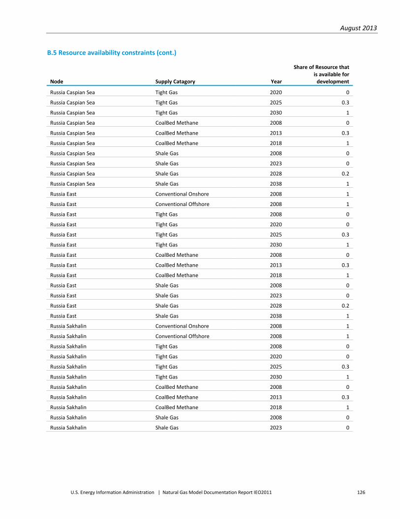
August 2013
U.S. Energy Information Administration | Natural Gas Model Documentation Report IEO2011 126
B.5 Resource availability constraints (cont.)
Node Supply Catagory Year
Share of Resource that is available for
development
Russia Caspian Sea Tight Gas 2020 0
Russia Caspian Sea Tight Gas 2025 0.3
Russia Caspian Sea Tight Gas 2030 1
Russia Caspian Sea CoalBed Methane 2008 0
Russia Caspian Sea CoalBed Methane 2013 0.3
Russia Caspian Sea CoalBed Methane 2018 1
Russia Caspian Sea Shale Gas 2008 0
Russia Caspian Sea Shale Gas 2023 0
Russia Caspian Sea Shale Gas 2028 0.2
Russia Caspian Sea Shale Gas 2038 1
Russia East Conventional Onshore 2008 1
Russia East Conventional Offshore 2008 1
Russia East Tight Gas 2008 0
Russia East Tight Gas 2020 0
Russia East Tight Gas 2025 0.3
Russia East Tight Gas 2030 1
Russia East CoalBed Methane 2008 0
Russia East CoalBed Methane 2013 0.3
Russia East CoalBed Methane 2018 1
Russia East Shale Gas 2008 0
Russia East Shale Gas 2023 0
Russia East Shale Gas 2028 0.2
Russia East Shale Gas 2038 1
Russia Sakhalin Conventional Onshore 2008 1
Russia Sakhalin Conventional Offshore 2008 1
Russia Sakhalin Tight Gas 2008 0
Russia Sakhalin Tight Gas 2020 0
Russia Sakhalin Tight Gas 2025 0.3
Russia Sakhalin Tight Gas 2030 1
Russia Sakhalin CoalBed Methane 2008 0
Russia Sakhalin CoalBed Methane 2013 0.3
Russia Sakhalin CoalBed Methane 2018 1
Russia Sakhalin Shale Gas 2008 0
Russia Sakhalin Shale Gas 2023 0

August 2013
U.S. Energy Information Administration | Natural Gas Model Documentation Report IEO2011 127
B.5 Resource availability constraints (cont.)
Node Supply Catagory Year
Share of Resource that is available for
development
Russia Sakhalin Shale Gas 2028 0.2
Russia Sakhalin Shale Gas 2038 1
Russia Shtokman Conventional Onshore 2008 1
Russia Shtokman Conventional Offshore 2008 1
Russia Shtokman Tight Gas 2008 0
Russia Shtokman Tight Gas 2020 0
Russia Shtokman Tight Gas 2025 0.3
Russia Shtokman Tight Gas 2030 1
Russia Shtokman CoalBed Methane 2008 0
Russia Shtokman CoalBed Methane 2013 0.3
Russia Shtokman CoalBed Methane 2018 1
Russia Shtokman Shale Gas 2008 0
Russia Shtokman Shale Gas 2023 0
Russia Shtokman Shale Gas 2028 0.2
Russia Shtokman Shale Gas 2038 1
Russia West Conventional Onshore 2008 1
Russia West Conventional Offshore 2008 1
Russia West Tight Gas 2008 0
Russia West Tight Gas 2020 0
Russia West Tight Gas 2025 0.3
Russia West Tight Gas 2030 1
Russia West CoalBed Methane 2008 0
Russia West CoalBed Methane 2013 0.3
Russia West CoalBed Methane 2018 1
Russia West Shale Gas 2008 0
Russia West Shale Gas 2023 0
Russia West Shale Gas 2028 0.2
Russia West Shale Gas 2038 1
Russia Yamal Conventional Onshore 2008 1
Russia Yamal Conventional Offshore 2008 1
Russia Yamal Tight Gas 2008 0
Russia Yamal Tight Gas 2020 0
Russia Yamal Tight Gas 2025 0.3
Russia Yamal Tight Gas 2030 1

August 2013
U.S. Energy Information Administration | Natural Gas Model Documentation Report IEO2011 128
B.5 Resource availability constraints (cont.)
Node Supply Catagory Year
Share of Resource that is available for
development
Russia Yamal CoalBed Methane 2008 0
Russia Yamal CoalBed Methane 2013 0.3
Russia Yamal CoalBed Methane 2018 1
Russia Yamal Shale Gas 2008 0
Russia Yamal Shale Gas 2023 0
Russia Yamal Shale Gas 2028 0.2
Russia Yamal Shale Gas 2038 1
South Korea Conventional Onshore 2008 1
South Korea Conventional Offshore 2008 1
South Korea Tight Gas 2008 0
South Korea Tight Gas 2020 0
South Korea Tight Gas 2025 0.3
South Korea Tight Gas 2030 1
South Korea CoalBed Methane 2008 0
South Korea CoalBed Methane 2018 0
South Korea CoalBed Methane 2023 0.3
South Korea CoalBed Methane 2028 1
South Korea Shale Gas 2008 0
South Korea Shale Gas 2023 0
South Korea Shale Gas 2028 0.2
South Korea Shale Gas 2038 1
US - Arctic Conventional Onshore 2008 1
US - Arctic Conventional Offshore 2008 1
US - Arctic Tight Gas 2008 1
US - Arctic CoalBed Methane 2008 0.75
US - Arctic CoalBed Methane 2014 0.75
US - Arctic CoalBed Methane 2024 1
US - Arctic Shale Gas 2008 1
US - AZNM Conventional Onshore 2008 1
US - AZNM Conventional Offshore 2008 1
US - AZNM Tight Gas 2008 1
US - AZNM CoalBed Methane 2008 0.75
US - AZNM CoalBed Methane 2014 0.75
US - AZNM CoalBed Methane 2024 1

August 2013
U.S. Energy Information Administration | Natural Gas Model Documentation Report IEO2011 129
B.5 Resource availability constraints (cont.)
Node Supply Catagory Year
Share of Resource that is available for
development
US - AZNM Shale Gas 2008 1
US - California Conventional Onshore 2008 1
US - California Conventional Offshore 2008 1
US - California Tight Gas 2008 1
US - California CoalBed Methane 2008 0.75
US - California CoalBed Methane 2014 0.75
US - California CoalBed Methane 2024 1
US - California Shale Gas 2008 1
US - East North Central Conventional Onshore 2008 1
US - East North Central Conventional Offshore 2008 1
US - East North Central Tight Gas 2008 1
US - East North Central CoalBed Methane 2008 0.75
US - East North Central CoalBed Methane 2014 0.75
US - East North Central CoalBed Methane 2024 1
US - East North Central Shale Gas 2008 1
US - East South Central Conventional Onshore 2008 1
US - East South Central Conventional Offshore 2008 1
US - East South Central Tight Gas 2008 1
US - East South Central CoalBed Methane 2008 0.75
US - East South Central CoalBed Methane 2014 0.75
US - East South Central CoalBed Methane 2024 1
US - East South Central Shale Gas 2008 1
US - Florida Conventional Onshore 2008 1
US - Florida Conventional Offshore 2008 1
US - Florida Tight Gas 2008 1
US - Florida CoalBed Methane 2008 0.75
US - Florida CoalBed Methane 2014 0.75
US - Florida CoalBed Methane 2024 1
US - Florida Shale Gas 2008 1
US - Middle Atlantic Conventional Onshore 2008 1
US - Middle Atlantic Conventional Offshore 2008 1
US - Middle Atlantic Tight Gas 2008 1
US - Middle Atlantic CoalBed Methane 2008 0.75
US - Middle Atlantic CoalBed Methane 2014 0.75

August 2013
U.S. Energy Information Administration | Natural Gas Model Documentation Report IEO2011 130
B.5 Resource availability constraints (cont.)
Node Supply Catagory Year
Share of Resource that is available for
development
US - Middle Atlantic CoalBed Methane 2024 1
US - Middle Atlantic Shale Gas 2008 1
US - Mountain Conventional Onshore 2008 1
US - Mountain Conventional Offshore 2008 1
US - Mountain Tight Gas 2008 1
US - Mountain CoalBed Methane 2008 0.75
US - Mountain CoalBed Methane 2014 0.75
US - Mountain CoalBed Methane 2024 1
US - Mountain Shale Gas 2008 1
US - New England Conventional Onshore 2008 1
US - New England Conventional Offshore 2008 1
US - New England Tight Gas 2008 1
US - New England CoalBed Methane 2008 0.75
US - New England CoalBed Methane 2014 0.75
US - New England CoalBed Methane 2024 1
US - New England Shale Gas 2008 1
US - Pacific Northwest Conventional Onshore 2008 1
US - Pacific Northwest Conventional Offshore 2008 1
US - Pacific Northwest Tight Gas 2008 1
US - Pacific Northwest CoalBed Methane 2008 0.75
US - Pacific Northwest CoalBed Methane 2014 0.75
US - Pacific Northwest CoalBed Methane 2024 1
US - Pacific Northwest Shale Gas 2008 1
US - South Atlantic Conventional Onshore 2008 1
US - South Atlantic Conventional Offshore 2008 1
US - South Atlantic Tight Gas 2008 1
US - South Atlantic CoalBed Methane 2008 0.75
US - South Atlantic CoalBed Methane 2014 0.75
US - South Atlantic CoalBed Methane 2024 1
US - South Atlantic Shale Gas 2008 1
US - West North Central Conventional Onshore 2008 1
US - West North Central Conventional Offshore 2008 1
US - West North Central Tight Gas 2008 1
US - West North Central CoalBed Methane 2008 0.75

August 2013
U.S. Energy Information Administration | Natural Gas Model Documentation Report IEO2011 131
B.5 Resource availability constraints (cont.)
Node Supply Catagory Year
Share of Resource that is available for
development
US - West North Central CoalBed Methane 2014 0.75
US - West North Central CoalBed Methane 2024 1
US - West North Central Shale Gas 2008 1
US - West South Central Conventional Onshore 2008 1
US - West South Central Conventional Offshore 2008 1
US - West South Central Tight Gas 2008 1
US - West South Central CoalBed Methane 2008 0.75
US - West South Central CoalBed Methane 2014 0.75
US - West South Central CoalBed Methane 2024 1
US - West South Central Shale Gas 2008 1

August 2013
U.S. Energy Information Administration | Natural Gas Model Documentation Report IEO2011 132
Appendix C. Database Description The INGM is implemented in Microsoft ACCESS using Visual Basic for Applications. This section defines the database tables that contain input, output, and intermediate output data.
Input data tables Symbol Field FDef Units
Table: tInp_AA_Base
This table stores the options for the base physical characteristics of the system such as fuels, nodes, regions, and seasons
AA_Base_Id Id of baseline physical characteristics option
AA_Base_Name Name of baseline physical characteristics option
Select_Flag Selection flag used for data input and review
Table: tInp_AA_Dmd_Spec
This table stores the options for the baseline demand
AA_DmdSpec_Id Id of baseline demand option
AA_DmdSpec_Name Name of baseline demand option
Select_Flag Selection flag used for data input and review
ScaleFlag Scale_Flag Flag set to true if demand is to be based on
another baseline demand option scaled and
false otherwise
AA_DmdSpec_Id_Base Id of baseline demand option to use for scaling
Table: tInp_AA_DmdSS
This table stores the options for the demand sectors and seasons specifications
AA_DmdSS_Id Id of baseline demand sector and season
option
AA_DmdSS_Name Name of baseline demand sector and season
option
Select_Flag Selection flag used for data input and review
Table: tInp_AA_ImpExp_Cnstr
This table stores the options for the import/export constraints
AA_ImpExp_Id Id of baseline import/export option
AA_ImpExp_Name Name of baseline import/export option
Select_Flag Selection flag used for data input and review
Table: tInp_AA_OthDmd
This table stores the options for the other fuel prices
AA_OthDmd_Id Id of baseline other fuel price option
AA_OthDmd_Name Name of other fuel price option
Select_Flag Selection flag used for data input and review

August 2013
U.S. Energy Information Administration | Natural Gas Model Documentation Report IEO2011 133
Symbol Field FDef Units
Table: tInp_AA_PipelineACnstr
This table stores the options for the pipeline assets
AA_PipelineACnstr_Id Id of pipeline asset option
AA_PipelineACnstr_Name Name of pipeline asset option
Select_Flag Selection flag used for data input and review
Table: tInp_AA_PorttoPort
This table stores the options for the port-to-port links in the network
AA_PorttoPort_Id Id of processing assets option
AA_PorttoPort_Name Name of processing assets option
Select_Flag Selection flag used for data input and review
Table: tInp_AA_ProcessingACnstr
This table stores the options for the processing assets
AA_ProcessingACnstr_Id
AA_ProcessingACnstr_Name
Select_Flag
Table: tInp_AA_StorageACnstr
This table stores the options for the storage assets
AA_StorageACnstr_Id Id of storage assets option
AA_StorageACnstr_Name Name of storage assets option
Select_Flag Selection flag used for data input and review
Table: tInp_AA_Supply
This table stores the options for the base natural gas resource estimates
AA_Supply_Id Id of baseline natural gas resource option
AA_Supply_Name
Name of baseline natural gas resource option
Select_Flag
Selection flag used for data input and review
Table: tInp_AA_TankerACnstr
This table stores the options for the tanker assets
AA_TankerACnstr_Id Id of tanker assets option
AA_TankerACnstr_Name Name of tanker assets option
Select_Flag Selection flag used for data input and review

August 2013
U.S. Energy Information Administration | Natural Gas Model Documentation Report IEO2011 134
Table: tInp_CTax
This table stores the baseline data for carbon taxes. The carbon tax data is defined by node in units of $2006/tonne CO2e.
AA_DmdSpec_Id Id of baseline demand option
n NodeId Unique id for node
y Year Year of the demand specification Year
CTaxn,y CTax Tax on CO2 assumed in the WEPS+ model and used to estimate the base demand $2006/tonne CO2e
CTax_Scenn,y CTax_Scen Tax on CO2 used in the INGM scenario $2006/tonne CO2e Table: tInp_DmdBase This table stores the baseline data for the demand. The demand data is defined by node and demand sector, and the data includes the base estimates of average daily demand for the year, node and demand sector in units of PJ/day.
AA_DmdSpec_Id Id of baseline demand option
n NodeId Unique id for node
f FuelId Unique ID for the fuel type
k DmdSectorId Unique Id for the demand sector
y Year Year of the demand specification Year
BDmdn,f,k,y BaseDmd
Base demand in year for node, fuel, and sector. Note that if data are not specified for a year then a value is interpolated between years where it is specified. If there are no values past some year then the last specified value is assumed PJ
BPron,f,k,y BasePrc
Base price for demand estimate. Note that if the value is not specified for a year then the value is interpolated between years where it is specified. If there are no values past some year then the last specified value is assumed $/GJ
BEffn,f,k,y BaseEff Base efficiency for demand sector for node, sector, fuel, and year Fraction
SPrcn,f,k,y ScnPrc Scenario price for scenario estimation $/GJ
BPrc_Orign,f,k,y BasePrc_Orig
Base price for demand estimate initially from the WEPS+model and before adjustment to nodal values $/GJ
PrcSubn,f,k,y PrcSub
Price subsidy assumed for the input demand assumptions for the wholesale price on average for the region $/GJ
PrcSubSn,f,k,y PrcSub_Scn
Price subsidy used to estimate demand for demand assumptions for the wholesale price on average for the region $/GJ
DstMarn,f,k,y DistMar Distribution Margin $/GJ
NFCstsn,f,k,y NFCstgs Non-fuel costs in using fuel $/GJ
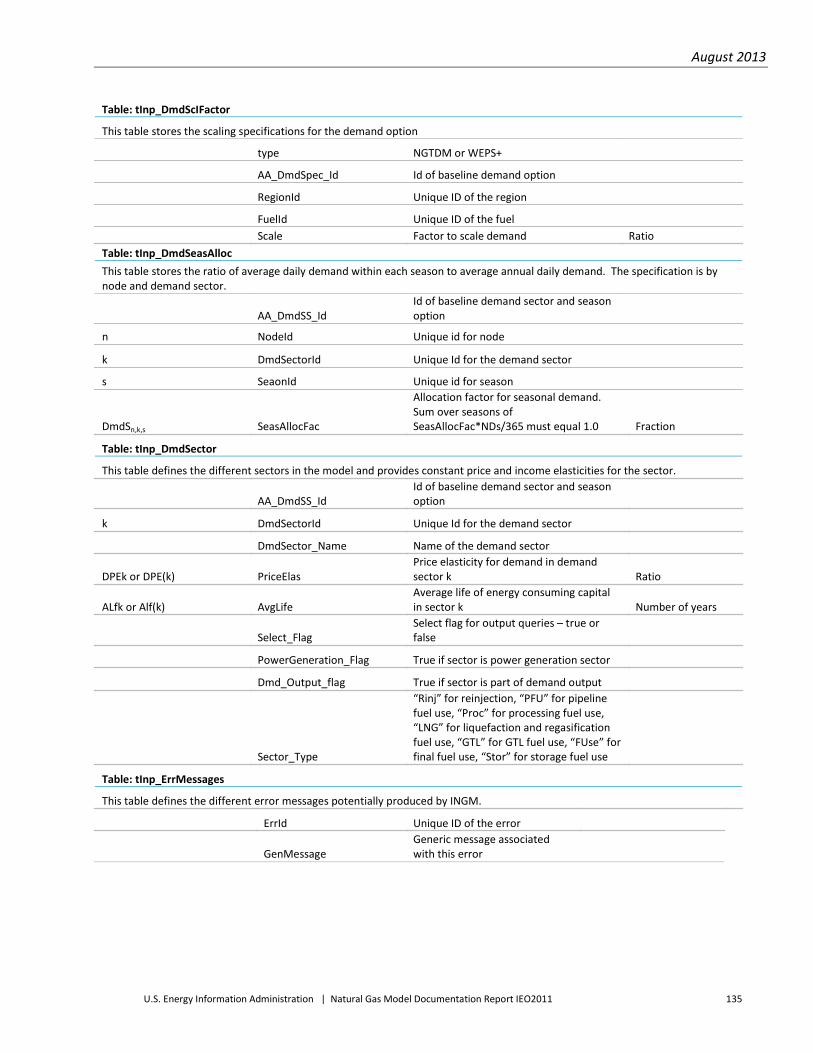
August 2013
U.S. Energy Information Administration | Natural Gas Model Documentation Report IEO2011 135
Table: tInp_DmdScIFactor
This table stores the scaling specifications for the demand option
type NGTDM or WEPS+
AA_DmdSpec_Id Id of baseline demand option
RegionId Unique ID of the region
FuelId Unique ID of the fuel Scale Factor to scale demand Ratio Table: tInp_DmdSeasAlloc This table stores the ratio of average daily demand within each season to average annual daily demand. The specification is by node and demand sector.
AA_DmdSS_Id Id of baseline demand sector and season option
n NodeId Unique id for node
k DmdSectorId Unique Id for the demand sector
s SeaonId Unique id for season
DmdSn,k,s SeasAllocFac
Allocation factor for seasonal demand. Sum over seasons of SeasAllocFac*NDs/365 must equal 1.0 Fraction
Table: tInp_DmdSector
This table defines the different sectors in the model and provides constant price and income elasticities for the sector.
AA_DmdSS_Id Id of baseline demand sector and season option
k DmdSectorId Unique Id for the demand sector
DmdSector_Name Name of the demand sector
DPEk or DPE(k) PriceElas Price elasticity for demand in demand sector k Ratio
ALfk or Alf(k) AvgLife Average life of energy consuming capital in sector k Number of years
Select_Flag Select flag for output queries – true or false
PowerGeneration_Flag True if sector is power generation sector
Dmd_Output_flag True if sector is part of demand output
Sector_Type
“Rinj” for reinjection, “PFU” for pipeline fuel use, “Proc” for processing fuel use, “LNG” for liquefaction and regasification fuel use, “GTL” for GTL fuel use, “FUse” for final fuel use, “Stor” for storage fuel use
Table: tInp_ErrMessages
This table defines the different error messages potentially produced by INGM.
ErrId Unique ID of the error
GenMessage Generic message associated with this error

August 2013
U.S. Energy Information Administration | Natural Gas Model Documentation Report IEO2011 136
Symbol Field FDef Units
Table: tInp_Fuel
This table defines the different fuel types used in INGM.
f FuelId Unique ID for the fuel type
Fuel_Name Name of the fuel
Select_Flag Select flag for output queries – true or false
CarCf CarContent CO2 content of the fuel Tonne CO2/GJ
Table: tInp_Fuel_Scn This table defines the different fuel types used in INGM for the base physical characteristics scenario. The field Flag indicates if the fuel is the produced gas (wet natural gas), dry gas consumed, NGL, or re-injected gas
AA_Base_Id Id of baseline physical characteristics option
f FuelId Unique ID for the fuel type
Flag
"D", "S", “N”, “R”, or "" indicting if the fuel is for demand (processed natural gas), supply (unprocessed natural gas), NGLs, re-injected gas, or other
Table: tGAMS_Dir
This table identifies the drive and directory of the GAMS file used when GAMS is used.
GAMS_DIR Directory where the GAMS files reside
Table: tInp_ImpExp_Cnstr This table defines the import and export constraints for the model. Each region can have a limit placed on net imports of natural gas or LNG and/or net exports of natural gas or LNG. Also, this table can be used to adjust production costs to reflect regional limits on the price allowed. These production cost limits can be defined with a fixed number or defined as a function of a fuel price.
AA_ImpExp_Id Id of baseline import/export option
r RegionId RegionId of region that the constraint applies to
y Year Year that the price applies Year
ImpLmtr,f,y ImpCnstr Annual limit on imports to the region and only used if FuelId is null EJ
ExpLmtr,f,y ExpCnstr Annual limit on exports from the region and only used if FuelId is null EJ
fp(r) FuelId Unique ID for the fuel type used to index the minimum price on
MnPrcIr MinPrc_Int Intercept for minimum price equation. Note that it is specified for only one year but applies to all $/GJ
MnPrcFr MinPrc_Fac
Factor for minimum price equation to be multiplied for price for specified fuel. Note that it is specified for only one year but applies to all Ratio
InvCr,y InvCnstr Investment costraint for the region and only used if FuelId is null Million $
EI_Cnstr,y MinCntrrFlag Flag if export/import constraint is annual and not seasonal True/False

August 2013
U.S. Energy Information Administration | Natural Gas Model Documentation Report IEO2011 137
Symbol Field FDef Units
Table: tInp_Node
This table defines the nodes used in INGM.
n NodeId Unique ID number for the node
Node_Name Name of the node
Select_Flag Select flag for output queries – true or false
usf(n) US_Flag Flag set to true if node is in the U.S.
naf(n) NA_Flag Flag set to true if the node is in North America
atlf(n) Atl_Flag Flag set to true if the node is on the Atlantic in North America
Table: tInp_Node_Scn
This table maps the nodes to the regions which are used for import/export constraints and reporting. It also specifies the government take for the node
AA_Base_Id Id of baseline physical characteristics option
n NodeId Unique ID number for the node
r(n) RegionId RegionId of region in which node n is located
PortCn Port_Capacity
The maximum number of ships in the port at any one time for loading or unloading – not currently used Number ships per day
Govtn GovtTake The government share of the natural gas sales price Fraction
PEffBn ProdIEffBase
Base Value for production inefficiency for node – reduces the share of economic resources that can be developed Fraction
PEffIn ProdIEffImp Annual improvement in production inefficiency value with total share capped at 1.0 Fraction/Year
OthFUn OthFU
Fraction of secondary demand used for internal pipelines and distribution and not captured in the specified pipelines Fraction
Rpt_RegionId IEO reporting region
GovtTake_Tx The government share of the natural gas sales price (fraction that is taxes – used for NGL sales
Table: tInp_OthDmd
This table defines the price that the market is willing to pay for other fuels. This is used to define the value of NGLs and GTL fuels.
AA_OthDmd_Id Id of baseline other fuel price option
f FuelId Unique ID for the fuel type
y Year Year that the price applies Year
OPrcf,y ODPrc Price of fuel in the market (applies only to NGLs, GTLs, and reinjected gas) $/GJ

August 2013
U.S. Energy Information Administration | Natural Gas Model Documentation Report IEO2011 138
Symbol Field FDef Units
Table: tInp_PipelineAsset
This table defines the pipelines used to transport dry gas between nodes. The specification includes the origin and destination nodes, fuel use in the transport, capacity costs, operating costs, and the life of different stages of the pipeline asset planning, construction, and operation.
p PipelineId Unique ID for the pipeline
Pipeline_Name Name of the pipeline
f(p) FuelId ID of fuel type that the pipeline transports
on(p) Org_NodeId NodeId of the node at the start of the pipeline
dn(p) Dst_NodeId NodeId of the node at the end of the pipeline
CapIp Capacity_Increment Capacity increment for capacity increases PJ/day
NYPp Num_Yrs_PlnAppr Number of years required for planning and approvals Number Years
PACstp PlanAppr_Cst Annual Planning and Approval costs $mil per year per capacity increment
NYCp Num_Yrs_Inv Number of years required for construction Number Years
ICstp Investment_Cost Investment cost per year $mil per year per capacity increment
MxLp Maximum_Life Maximum operating life of asset (e.g., 30 years) Number Years
FOaMCp Fixed_OaM_Cost Annual fixed operating and maintenance cost per year
$mil per year per capacity increment
VOaMCp Variable_OaM_Cost Variable Operating and Maintenance Cost $/GJ
FUp Fuel_Use Pipeline fuel use fraction
RCstp Retirement_Cost Cost of retiring the asset $mil per year per capacity increment
Select_Flag Select flag for output queries – true or false
Table: tInp_PipelineAsset_Cnstr This table defines the constraints on pipeline capacity. Existing capacity or new capacity that is firm is defined with minimum and maximum capacity set equal to the capacity value. New capacity is only built in a year if a capacity expansion record exists for the pipeline covering the year.
AA_PipelineACnstr_Id Id of pipeline asset option
P PipelineId ID for the pipeline that the constraint applies to
X x is an index representing a year where FYear < x < LYear Year
sy FYear First year that following data apply for (e.g., 2006) Year
EYp,sy LYear Last year that following data apply for (e.g., 2010) – inclusive Year
MnCapp,sy Min_Capacity Minimum capacity addition allowed for the pipeline
PJ/day of input fuel to pipeline
MxCapp,sy Max_Capacity Maximum capacity addition allowed for the pipeline
PJ/day of input fuel to pipeline

August 2013
U.S. Energy Information Administration | Natural Gas Model Documentation Report IEO2011 139
Symbol Field FDef Units
Table: tInp_PorttoPort
This table defines the node to node routes for LNG tankers. This includes the number of days required for a one-way trip.
AA_PorttoPort_Id Id of port-to-port option
l PorttoPortId Id of Port-to-port link
PorttoPort_Name Name of Port-to-Port link
on(l) Org_NodeId NodeId of one end of the link
dn(l) Dst_NodeId NodeId of the other end of the link
TrpDl TripDuration Duration of trip Days
Select_Flag Select flag for output queries – true or false
TripDuration_Basis – unadjusted estimates which are not used Duration of trip Days
Suez Flag if trip is through Suez canal True/False
Panama Flag if trip is through Panama canal True/False
mnfflg(l) MinFlow_Flag
Flag if minimum flow is to be assigned to the port-to-port link and is used to control prices for the NGTDM interface. The minimum flow 1e-7 PJ tanker capacity Yes/No
Table: tInp_ProcessingAsset
This table defines the processing assets used to convert gas from one form to another. Processing assets include gas processing, liquefaction, regasification, and GTL technology. The specification includes the asset type, capacity costs, operating costs, and the life of different stages of the processing asset planning, construction, and operation.
a AssetId Unique ID number for the Asset
Asset_Name Asset Name
Asset_TypeID AssetID for asset type
CapIa Capacity_Increment Capacity increments required for investment
PJ/day of primary output fuel
f(a) FuelId Id of primary output fuel (capacity is measure on output of this fuel)
NYPa Num_Yrs_PlnAppr Number of years required for planning and approvals Number Years
PACsta PlanAppr_Cst Annual Planning and Approval costs
$mil per year per capacity increment
NYCa Num_Yrs_Inv Number of years required for construction Number Years
ICsta Investment_Cost Investment cost per year
$mil per year per capacity increment
MxLa Maximum_Life Maximum operating life of asset (e.g., 30 years) Number Years
FOaMCa Fixed_OaM_Cost Annual fixed operating and maintenance cost per year
$mil per year per capacity increment
VOaMCa Variable_OaM_Cost Variable Operating and Maintenance Cost $/GJ

August 2013
U.S. Energy Information Administration | Natural Gas Model Documentation Report IEO2011 140
Symbol Field FDef Units
RCsta Retirement_Cost Cost of retiring the asset $mil per year per capacity increment
Select_Flag Select flag for output queries – true or false
Table: tInp_ProcessingAsset_Fuel
This table defines the input energy and output energy by fuel type for each processing asset. The input and output fuel quantities should be defined consistent with the capacity increment of the asset and the quantity for the primary output fuel should equal the capacity increment. For example, if a processing asset takes 1 PJ/day of unprocessed gas and produces 0.95 PJ/day of processed gas and 0.03 PJ/day of NGLS then this table should have three records – one for the input fuel at 1PJ/day and two for the output fuels with 0.95 and 0.03 PJ/day. The capacity increment should be 0.95 PJ/day.
a AssetId AssetID for asset that data apply to
f Fuelid FuelId of the fuel that data apply to Long
Qtya,f Qty Quantity input (negative) or output (positive) for capacity increment PJ/day
Table: tInp_ProcessingAsset_RegCnstr
This table defines the constraints on processing capacity. Existing capacity or new capacity that is firm is defined with minimum and maximum capacity set equal to the capacity value. New capacity is only built in a year if a capacity expansion record exists for the processing asset for the node covering the year.
AA_ProcessingACnstr_Id Id of processing assets option
n NodeId Unique ID number for the Node
a AssetId Unique ID number for the Asset
x x is an index representing a year where FYear < x < LYear Year
sy FYear First year that following data apply for (e.g., 2006) Year
EYn,a,sy LYear Last year that following data apply for (e.g., 2010) – inclusive Year
MnCapn,a,sy Min_Capacity Minimum capacity addition allowed in the node PJ/day output of primary fuel
MxCapn,a,sy Max_Capacity Maximum capacity addition allowed in the node PJ/day output of primary fuel
Symbol Field FDef Units
Table: tInp_ProcessingAsset_Type
This table defines the different processing asset types (e.g., liquefaction)
Asset_TypeID Unique AssetID for asset type
Asset_Type_Name Name
Select_Flag Selection flag used for data input and review
Asset_Type "LNG" for liquefaction or regasification, "Proc" for gas processing, "GTL" for GTL plant
Table: tInp_PScalar
This table defines the price scalar by year and for each asset type
Symbol Field FDef Units

August 2013
U.S. Energy Information Administration | Natural Gas Model Documentation Report IEO2011 141
b PS_Type Asset type (Pipeline, Production, ProcAsset, Storage, or Tanker)
0 for production, 1 for pipeline, 2 for processing asset, 3 for tanker, and 4 for storage
y Year Year of the cost scalar Year
PScalarb,y PScalar
Cost scalar reflecting both increases in asset/production costs and technological improvement Ratio
Table: tInp_Region
This table defines the different regions.
r RegionId Unique ID number for the region
Region_Name Name of the region
Select_Flag Select flag for output queries – true or false
usf(r) US_Flag Flag set to true if region is in the U.S.
naf(r) NA_Flag Flag set to true if the region is in North America
Table: tInp_Region_Scn
This table defines discount rates for the different regions.
AA_Base_Id Id of baseline physical characteristics option
r RegionId Unique ID number for the region
DRr DRate Discount rate for the region fraction
rc(r) CmbImpExp_RegionId Id of Region used as aggregate region for combined import/export constraint
Agr_RegionId Aggregate region for the WEPS+ output
Table: tRpt_Region
This table defines the different regions for output reports, without any subcountry groupings.
Rpt_RegionId Unique ID for the region
Rpt_Region_Name Name of the region
Table: tInp_Scenario
This table defines the different scenarios to run.
ScenarioID Unique ID number for the scenario
Scenario_Name Name of the scenario
SYear Start_Year First year of optimization Year
EYear End_Year Last year of optimization Year
TStep Time_Step Number of years between optimizations Years

August 2013
U.S. Energy Information Administration | Natural Gas Model Documentation Report IEO2011 142
Symbol Field FDef Units
AA_Base_Id Id of baseline physical characteristics option
AA_DmdSpec_Id Id of baseline demand option
AA_DmdSS_Id Id of baseline demand sector and season option
AA_ImpExp_Id Id of baseline import/export option
AA_OthDmd_Id Id of baseline other fuel price option
AA_PipelineACnstr_Id Id of pipeline asset option
AA_PorttoPort_Id Id of port-to-port option
AA_ProcessingACnstr_Id
Id of processing assets option
AA_StorageACnstr_Id Id of storage assets option
AA_Supply_Id Id of baseline natural gas resource option
AA_TankerACnstr_Id Id of tanker assets option
DRate DRate Global discount rate Fraction (.12 is 12%)
Select_Flag Select flag for output queries – true or false
StorFrac Storage_Fraction Fraction of storage working gas that can be effectively used.
Fraction
WEPS_Output_Scen Flag if scenario used to create WEPS+ output regression model
Table: tInp_Season
This table defines the different seasons.
s SeasonId Unique ID number for the season
Season_Name Name of the season
Select_Flag Select flag for output queries – true or false
Table: tInp_Season_Scn
This table defines the number of days in the seasons. The number of days in the seasons should add to 365.
AA_Base_Id Id of baseline physical characteristics option
s SeasonId Unique ID number for the season
NDs NumDays Number of days in the season Days
Table: tInp_StorageAsset This table defines the storage assets used for seasonal storage. The specification includes the asset type, capacity costs, operating costs, and the life of different stages of the storage asset planning, construction, and operation.
g StorageId Unique ID number for the Asset
Storage_Name Asset Name
CapIg Capacity_Increment Capacity increments required for investment EJ of working capacity

August 2013
U.S. Energy Information Administration | Natural Gas Model Documentation Report IEO2011 143
Symbol Field FDef Units
f(g) FuelId Id of fuel type storded
NYPg Num_Yrs_PlnAppr Number of years required for planning and approvals Number Years
PACstg PlanAppr_Cst Annual Planning and Approval costs $mil per year
NYCg Num_Yrs_Inv Number of years required for construction Number Years
ICstg Investment_Cost Investment cost per year $mil per year
MxLg Maximum_Life Maximum operating life of asset (e.g., 30 years) Number Years
FOaMCg Fixed_OaM_Cost Annual fixed operating and maintenance cost $mil per year
VOaMCg Variable_OaM_Cost Variable Operating and Maintenance Cost $/GJ
RCstg Retirement_Cost Cost of retiring the asset $mil
FUg Fuel use
Fuel use from the injection and withdrawal and including losses applied on injections
Fraction as a percentage of injections
Select_Flag Select flag for output queries – true or false
Table: tInp_StorageAsset_RegCnstr
This table defines the constraints on storage capacity. Existing capacity or new capacity that is firm is defined with minimum and maximum capacity set equal to the capacity value. New capacity is only built in a year if a capacity expansion record exists for the storage type and node covering the year.
AA_StorageACnstr_Id Id of storage assets option
n NodeId Unique ID number for the Node
g StorageId Unique ID number for the Asset
x x is an index representing a year where FYear < x < LYear Year
sy FYear First year that following data apply for (e.g., 2006) Year
EYn,g,sy LYear Last year that following data apply for (e.g., 2010) – inclusive Year
MnCapn,g,sy Min_Capacity Minimum capacity addition allowed in the node PJ working gas
MxCapn,g,sy Max_Capacity Maximum capacity addition allowed in the node PJ working gas
Table: tInp_SupplyBase
This table specifies the natural gas reserves and resources by node and major price step.
AA_Supply_Id Id of baseline natural gas resource option
n NodeId Unique id for node
c SupCatId Unique Id for the supply category – Note set to “All” now

August 2013
U.S. Energy Information Administration | Natural Gas Model Documentation Report IEO2011 144
Symbol Field FDef Units
m SMPrcStep Major price step for supply category (0, 1, 2, …)
BRsvn,c BYrRsv Base year reserves EJ
BURsn,c BYrURes Base year undeveloped resources EJ
MnPn,c,m MnPrc Minimum development costs at which reserves come online $/GJ
MxPn,c,m MxPrc Maximum development costs at which reserves come online $/GJ
αn,c,m SPVFac Supply curve price/volume factor
VPCn,c,m VrPrdCosts Variable production costs $/GJ
RsvSn,c,m RsvShr Share of economic/undeveloped resources that can be developed in the year Fraction
PRn,c,m PR_Ratio Maximum production to reserves ratio ratio
NPSn,c,m Num_MinPrcStp Number of minor price steps within major price step number
m(n,c,i) Major price step that the minor price step is part of
Sn,c,j
The incremental order of the minor price step within the major price step. For example if 16 is the first minor price step for major price step 4 and 20 is the last minor price step for price step 4 then s(n,c,16) is 1 and s(n,c,20) is 5.
NGLFn,c,m NGL_Frac Fraction of wet gas that is NGLs Fraction
Table: tInp_SupplyCat
This table defines the different supply categories (e.g., conventional onshore or tight gas) used in reporting.
c SupCatId Unique Id for the supply category
SupCat_Name
Name of the supply category (allow for All for common modelling of all supply categories simultaneously)
Select_Flag Select flag for output queries – true or false
Table: tInp_SupplyCatAsgn
This table specifies the share of undiscovered resources by supply category for each node and major price step.
AA_Supply_Id Id of baseline natural gas resource option
n NodeId Unique id for node
c SupCatId Unique Id for the supply category
m SMPrcStep Major price step for supply category (0, 1, 2, …)
URShrn,c,m Share
Share of reserves and undiscovered resources by node and major price step represented by supply category. Fraction

August 2013
U.S. Energy Information Administration | Natural Gas Model Documentation Report IEO2011 145
Table: tInp_TankerAsset
This table defines the tanker assets used for LNG transport. The specification includes the tanker type, capacity costs, operating costs, and the life of different stages of the tanker asset planning, construction, and operation. Tankers can also include onboard regasification capabilities and this table includes a field indicating if it does.
t TankerId Unique ID for the tanker type
Tanker_Name Name of the tanker type
CapIt Capacity_Increment Capacity increment for capacity increases – adjusted for expected utilization Pj per ship
NYPt Num_Yrs_PlnAppr Number of years required for planning and approvals
Number Years
PACstt PlanAppr_Cst Annual Planning and Approval costs $mil per year per ship
NYCt Num_Yrs_Inv Number of years required for construction Number Years
ICstt Investment_Cost Investment cost per year $mil per year per ship
MxLt Maximum_Life Maximum operating life of asset (e.g., 30 years) Number Years
FOaMCt Fixed_OaM_Cost Annual fixed operating and maintenance cost $mil per year per ship
VOaMCt Variable_OaM_Cost Variable Operating and Maintenance Cost $ per GJ per day
RCstt Retirement_Cost Cost of retiring the asset
$mil per year per capacity increment
RGFt Regas_Cap Flag is True if tanker has regasification capability built onboard True/False
LdTt Loading Time The number of days required to load the ship Days
UnLdTt Unloading Time The number of days required to unload the ship Days
Select_Flag Select flag for output queries – true or false
Capacity_Increment_Orig Capacity increment for capacity increases - unadjusted Pj per ship
Symbol Field FDef Units Table: tInp_SupplyCatCnst This table specifies the share of undiscovered resources by supply category for each node that is available to be developed in any year.
AA_Supply_Id Id of baseline natural gas resource option
n NodeId Unique id for node
c SupCatId Unique Id for the supply category
y Year
CCnstn,c,y Availability
Share of reserves and undiscovered resources by node and by supply category that is available to be developed in specified year. Note that if data are not specified for a year then a value is interpolated between years where it is specified. If there are no values past some year then the last specified value is assumed Fraction

August 2013
U.S. Energy Information Administration | Natural Gas Model Documentation Report IEO2011 146
Symbol Field FDef Units
Table: tInp_TankerAsset_Cnstr
This table defines the constraints on tanker capacity. Existing capacity or new capacity that is firm is defined with minimum and maximum capacity set equal to the capacity value. New capacity is only built in a year if a capacity expansion record exists for the tanker covering the year.
AA_TankerACnstr_Id Id of tanker assets option
t TankerId ID for the tanker type that the constraint applies to
x x is an index representing a year where FYear < x < LYear Year
sy FYear First year that following data apply for (e.g., 2006) Year
EYt,sy LYear Last year that following data apply for (e.g., 2010) – inclusive Year
MnCapt,sy Min_Capacity Minimum capacity addition allowed for the tanker type Number of ships
MxCapt,sy Max_Capacity Maximum capacity addition allowed for the tanker type Number of ships
Table: tInp_TankerFuel
This table defines the input and output fuels for each tanker. Typically they will be the same except for tankers with regasification capacity built in.
t TankerId ID for the tanker type that the constraint applies to
Inpf(t) Inp_FuelId Id of input fuel to tanker
Outf(t) Out_FuelId Id of output fuel to tanker corresponding to input fuel
Table: tInp_TankerPort
This table defines for each tanker type, the nodes that the tanker can import to or export from.
t TankerId ID for the tanker type that the constraint applies to
n NodeId NodeId of the port
TPFt,n Tanker_Port_Flag Flag set to true if tanker allowed in port and false (or not specified) otherwise True/False
Table: tInp_TimeStep
This table defines for the time steps for the rolling optimization.
TimeStep Number for time step which must start at 1 and be consecutive Integer
NumYears Number of years in the time step Years

August 2013
U.S. Energy Information Administration | Natural Gas Model Documentation Report IEO2011 147
Debug tables Field Description Units
Table: tMatrix_Coef This table stores the coefficients of the LP. The row, 0, contains the objective value and the column 0 contains the right hand side.
Row Row number of LP matrix where row 0 is the objective values Number
Col Column number of LP matrix where column 0 is the right hand side Number
Coef Coefficient in the LP matrix Varies depending on the column and row
Table: tMatrix_Col This table stores the definition of the columns in the LP and includes upper and lower bound of the column, the name of the column, the column number, and the value for the column in the optimal solution.
Col Column number of LP matrix where column 0 is the right hand side Number
Name Name of the Column
Lower_Bnd Lower bound of the column Varies depending on the column
Upper_Bnd Upper bound of the column Varies depending on the column
Solution LP solution Varies depending on the column
Table: tMatrix_Row This table stores the definition of the rows in the LP and includes the sense of the row, the name of the row, the row number, and the dual of the row and slack for the row in the results.
Row Row number of LP matrix where row 0 is the objective values Number
Name Name of the row
Sense “<”, “=”, “>”, or Null
Slack Slack in the solution for the row Varies depending on the column
Dual Dual of the row in the solution Varies depending on the column

August 2013
U.S. Energy Information Administration | Natural Gas Model Documentation Report IEO2011 148
Output tables Field Description Units
Table: tOut_Dmd
This table stores the output average annual demand by node and demand sector.
ScenarioID Unique ID number for the scenario
SYear First year of the optimization period Year
NodeID Unique ID of the node
DmdSectorId Unique Id for the demand sector
Year Year that the solution data applies to Year
Qty Demand in the solution. Note that this number multiplied by the seasonal factor provide seasonal demand in PJ/day PJ/day
FnlFlag Flag set to yes/true if data represents final solution for year True/False
Table: tOut_DmdOth
This table stores the natural gas fuel use demands by node, demand sector and season.
ScenarioID Unique ID number for the scenario
SYear First year of the optimization period Year
NodeID Unique ID of the node
DmdSectorId Unique Id for the demand sector
Year Year that the solution data applies to Year
SeasonId Unique Id for the season
Qty Demand in PJ/day PJ/day
FnlFlag Flag set to yes/true if data represents final solution for year True/False
Table: tOut_EOYRsv
This table stores the output end of year reserves for each supply category and major price step by node.
ScenarioID Unique ID number for the scenario
SYear First year of the optimization period Year
NodeID Unique ID of the node
SupCatId Unique Id for the supply category (should be supply category for “All”)
SMPrcStep Major price step Number
Year Year that the solution data applies to Year
Qty End of year remaining undiscovered resources in the solution. EJ
FnlFlag Flag set to yes/true if data represents final solution for year True/False
Table: tOut_ErrLog
This table stores any error messages produced by an INGM run.
ScenarioId Unique ID for the scenario
MsgNum Number of the message for the run
ErrId Unique ID of the error
Message Unique message associated with this error and occurrence of the error

August 2013
U.S. Energy Information Administration | Natural Gas Model Documentation Report IEO2011 149
Field Description Units
Table: tOut_NetCshFlw
This table stores the output net cash flow from investments and operations.
ScenarioID Unique ID number for the scenario
SYear First year of the optimization period Year
RegionID Unique ID of the region
Year Year that the solution data applies to Year
NCI Net cash flow for asset investments $mil
NCO Net cash flow from other activities (production, O&M, sales of products) $mil
FnlFlag Flag set to yes/true if data represents final solution for year True/False
ImpExpDual Dual from fixed import/export constraint $mil
Table: tOut_OthDmd
This table stores the output demand for non-natural gas fuels such as GTL diesel and NGLs.
ScenarioID Unique ID number for the scenario
SYear First year of the optimization period Year
NodeID Unique ID of the node
FuelID Unique ID of the fuel sold
Year Year that the solution data applies to Year
SeasonID Unique ID of the season
Qty Quantity fuel sold PJ/day
FnlFlag Flag set to yes/true if data represents final solution for year True/False

August 2013
U.S. Energy Information Administration | Natural Gas Model Documentation Report IEO2011 150
Field Description Units
Table: tOut_Pipe_Capacity
This table stores the output capacity installed for pipelines.
ScenarioID Unique ID number for the scenario
SYear First year of the optimization period Year
PipelineID Unique ID of the pipeline
Year Year that the solution data applies to Year
Cap Capacity that comes online in the year, measured as inflow to the pipeline PJ/day
CumCap Cumulative capacity online in the year, measured as inflow to the pipeline PJ/day
FnlFlag Flag set to yes/true if data represents final solution for year True/False
Table: tOut_Pipe_Utilization
This table stores the output utilization of the pipelines (in terms of fuel into the pipeline)
ScenarioID Unique ID number for the scenario
SYear First year of the optimization period Year
PipelineID Unique ID of the pipeline
Year Year that the solution data applies to Year
SeasonID Unique ID of the season
Utl Capacity utilization in season PJ/day
FnlFlag Flag set to yes/true if data represents final solution for year True/False
Table: tOut_Prices This table stores the prices for each fuel in each node by year. The price represents a weighted average price based on demand for the fuel.
ScenarioID Unique ID number for the scenario
SYear First year of the optimization period Year
NodeID Unique ID of the node
FuelID Unique ID of the fuel sold
Year Year that the solution data applies to Year
Price Average annual market price of the fuel weighted by total demand by season $/GJ
FnlFlag Flag set to yes/true if data represents final solution for year True/False
Table: tOut_Prices_Season
This table stores the prices for each fuel in each node by year and season.
ScenarioID Unique ID number for the scenario
SYear First year of the optimization period Year
NodeID Unique ID of the node
FuelID Unique ID of the fuel sold
Year Year that the solution data applies to Year
SeasonID Unique ID of the season
Price Average market price of the fuel for the season $/GJ
FnlFlag Flag set to yes/true if data represents final solution for year True/False

August 2013
U.S. Energy Information Administration | Natural Gas Model Documentation Report IEO2011 151
Field Description Units
Table: tOut_Proc_Capacity
This table stores the output capacity installed for gas processing assets.
ScenarioID Unique ID number for the scenario
SYear First year of the optimization period Year
NodeID Unique ID of the node
AssetID Unique ID of the asset
Year Year that the solution data applies to Year
Cap Capacity that comes online in the year, measured in output of primary fuel PJ/day
FnlFlag Flag set to yes/true if data represents final solution for year True/False
Table: tOut_Proc_Utilization
This table stores the utilization of the processing capacity measured in PJ/day of primary output fuel.
ScenarioID Unique ID number for the scenario
SYear First year of the optimization period Year
NodeID Unique ID of the node
AssetID Unique ID of the asset
Year Year that the solution data applies to Year
SeasonID Unique ID of the season
Utl Utilization of the capacity in the year and season, measured as output of primary fuel PJ/day
FnlFlag Flag set to yes/true if data represents final solution for year True/False
Table: tOut_Production
This table stores the output production by node, year, and season.
ScenarioID Unique ID number for the scenario
SYear First year of the optimization period Year
NodeID Unique ID of the node
SupCatId Unique ID of the supply category
SMPrcStep Major price step for supply category (0, 1, 2, …)
Year Year that the solution data applies to Year
SeasonID Unique ID of the season
Qty Production in the year and season including NGLs and reinjection gas PJ/day
ReInject Gas reinjected in year and season PJ/day
APrd Accelerated production in year and season PJ/day
FnlFlag Flag set to yes/true if data represents final solution for year True/False
Table: tOut_Production_Ann
This table stores the output production by node and year.
ScenarioID Unique ID number for the scenario
SYear First year of the optimization period Year
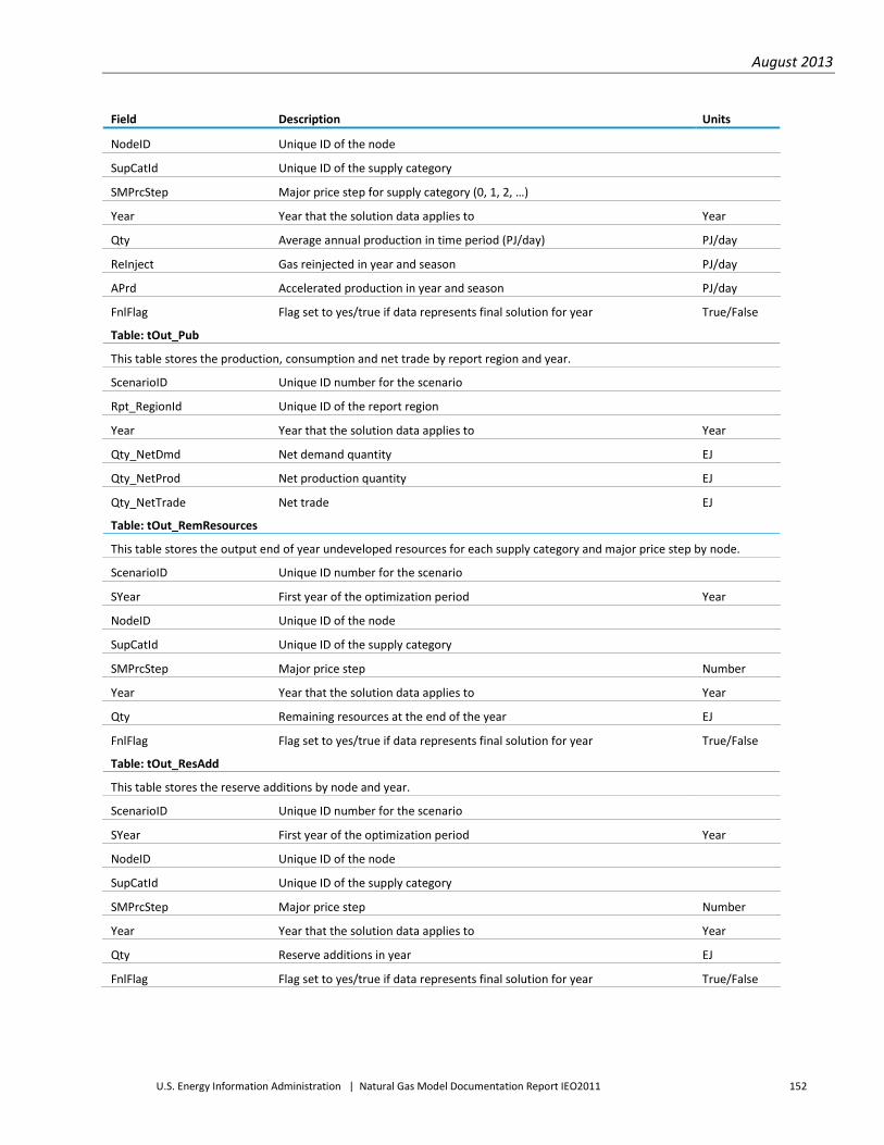
August 2013
U.S. Energy Information Administration | Natural Gas Model Documentation Report IEO2011 152
Field Description Units
NodeID Unique ID of the node
SupCatId Unique ID of the supply category
SMPrcStep Major price step for supply category (0, 1, 2, …)
Year Year that the solution data applies to Year
Qty Average annual production in time period (PJ/day) PJ/day
ReInject Gas reinjected in year and season PJ/day
APrd Accelerated production in year and season PJ/day
FnlFlag Flag set to yes/true if data represents final solution for year True/False
Table: tOut_Pub
This table stores the production, consumption and net trade by report region and year.
ScenarioID Unique ID number for the scenario
Rpt_RegionId Unique ID of the report region
Year Year that the solution data applies to Year
Qty_NetDmd Net demand quantity EJ
Qty_NetProd Net production quantity EJ
Qty_NetTrade Net trade EJ
Table: tOut_RemResources
This table stores the output end of year undeveloped resources for each supply category and major price step by node.
ScenarioID Unique ID number for the scenario
SYear First year of the optimization period Year
NodeID Unique ID of the node
SupCatId Unique ID of the supply category
SMPrcStep Major price step Number
Year Year that the solution data applies to Year
Qty Remaining resources at the end of the year EJ
FnlFlag Flag set to yes/true if data represents final solution for year True/False
Table: tOut_ResAdd
This table stores the reserve additions by node and year.
ScenarioID Unique ID number for the scenario
SYear First year of the optimization period Year
NodeID Unique ID of the node
SupCatId Unique ID of the supply category
SMPrcStep Major price step Number
Year Year that the solution data applies to Year
Qty Reserve additions in year EJ
FnlFlag Flag set to yes/true if data represents final solution for year True/False

August 2013
U.S. Energy Information Administration | Natural Gas Model Documentation Report IEO2011 153
Field Description Units
Table: tOut_Stor_Cap
This table stores the output storage capacity additions by year, node, and storage type.
ScenarioID Unique ID number for the scenario
SYear First year of the optimization period Year
NodeID Unique ID of the node
StorageId Unique ID of the storage type
Year Year that the capacity comes online Year
Cap Capacity, working gas, that comes online in the year PJ
FnlFlag Flag set to yes/true if data represents final solution for year True/False
Table: tOut_Stor_Utilization This table stores the output storage utilization by node, year, season, and storage type. The utilization includes injections and withdrawals.
ScenarioID Unique ID number for the scenario
SYear First year of the optimization period Year
NodeID Unique ID of the node
StorageId Unique ID of the storage type
Year Year that the solution data applies to Year
SeasonID Unique ID of the season
Inj Quantity injected during season PJ/day
Wth Quantity extracted during season PJ/day
FnlFlag Flag set to yes/true if data represents final solution for year True/False
Table: tOut_SupplyCatAsgn
This table stores the share of reserves/resources by node, supply category and major price step for each year.
ScenarioId Unique ID number for the scenario
NodeId Unique Id number for the node
SupCatId Unique Id for the supply category
SMPrcStep Major price step for the supply category (0 to n)
Year Year
Share Share of reserves/resources in the category for production and reserves Fraction
ShareRA Share of reserves/resources in the category for reserve additions Fraction
ShareRR Share of reserves/resources in the category for remaining reserves Fraction
SYear Start year of the optimization period
FnlFlag Flag set to yes if data represents final solution for year True/False
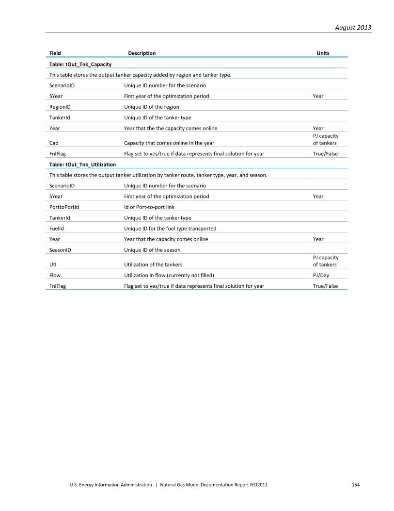
August 2013
U.S. Energy Information Administration | Natural Gas Model Documentation Report IEO2011 154
Field Description Units
Table: tOut_Tnk_Capacity
This table stores the output tanker capacity added by region and tanker type.
ScenarioID Unique ID number for the scenario
SYear First year of the optimization period Year
RegionID Unique ID of the region
TankerId Unique ID of the tanker type
Year Year that the the capacity comes online Year
Cap Capacity that comes online in the year PJ capacity of tankers
FnlFlag Flag set to yes/true if data represents final solution for year True/False
Table: tOut_Tnk_Utilization
This table stores the output tanker utilization by tanker route, tanker type, year, and season.
ScenarioID Unique ID number for the scenario
SYear First year of the optimization period Year
PorttoPortId Id of Port-to-port link
TankerId Unique ID of the tanker type
FuelId Unique ID for the fuel type transported
Year Year that the capacity comes online Year
SeasonID Unique ID of the season
Utl Utilization of the tankers PJ capacity of tankers
Flow Utilization in flow (currently not filled) PJ/Day
FnlFlag Flag set to yes/true if data represents final solution for year True/False

August 2013
U.S. Energy Information Administration | Natural Gas Model Documentation Report IEO2011 155
Appendix D Programmers Guide The INGM is implemented in Visual Basic within Microsoft ACCESS and through the use of predefined queries for output. The code is contained in eleven modules each focusing on specific tasks as follows:
• mAdjustBasePrice – adjusts the input regional demand prices based on existing nodal prices • mBuildMatrix – Builds the LP matrix • mCleanOutputRslts – Provides utility routines for cleaning out the output tables • mDocument – Provides summary of database tables for documentation • mINGM_Main – Main routine for INGM and controls looping, input, processing, and output • mLPSetUp – Utility routines for setting up the matrix and building the MPS file for the commercial
solver • mOutputQueries – Routines that build the output queries for the report writer • mReadData – Reads the input data and scenario specifications and stores them in arrays • mReadMPSRslt – Reads in the output from CPLEX or GAMS and stores in arrays • mRefIntegrity – Maintenance routines that test the referential integrity of the input data sets • mShellWait – Utility routine used to control the running of the commercial solver
Module: mAdjustBasePrice
Main Routines iCorrectNodalBasePrices
Description: The function takes the input nodal prices, which are essentially more aggregate regional averages from the WEPS+ model, and adjusts them based on nodal prices from a previous INGM run.
Input:
lScenarioId – index of the previously run model scenario, the results from which are to be used to adjust the new demand prices
lDmdSpecId –index of the demand inputs for which prices are to be adjusted
Functions Used: None
Return Output: None
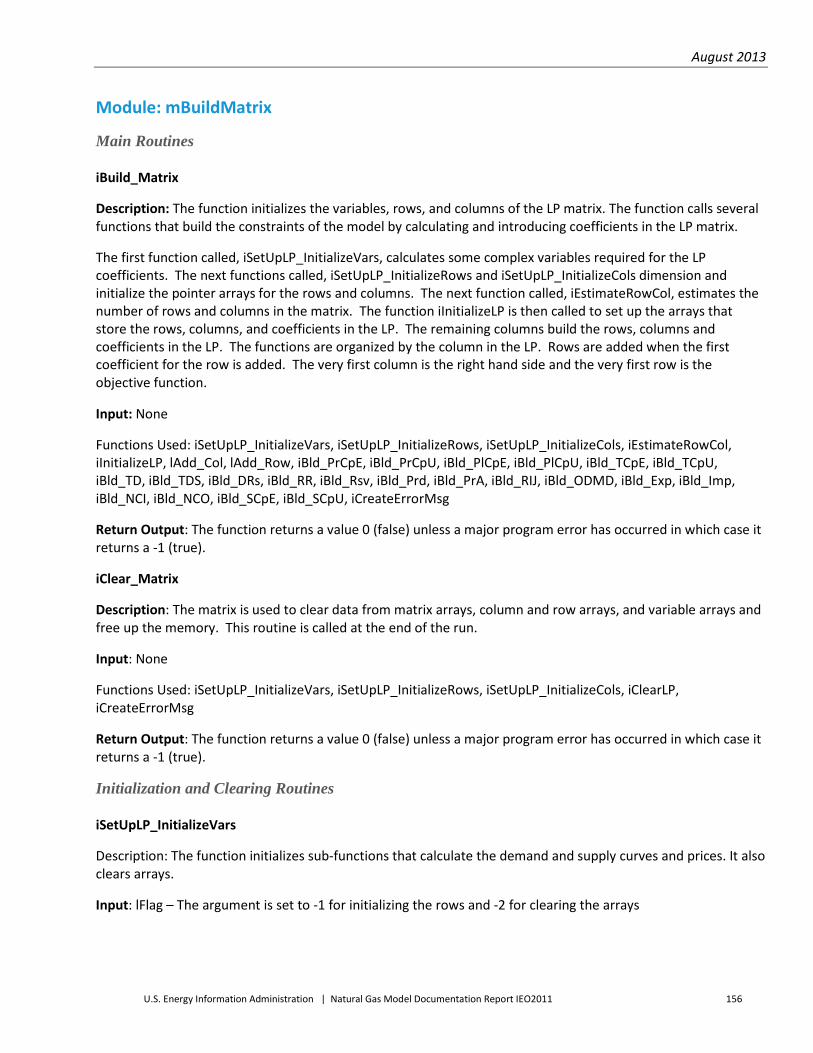
August 2013
U.S. Energy Information Administration | Natural Gas Model Documentation Report IEO2011 156
Module: mBuildMatrix
Main Routines iBuild_Matrix
Description: The function initializes the variables, rows, and columns of the LP matrix. The function calls several functions that build the constraints of the model by calculating and introducing coefficients in the LP matrix.
The first function called, iSetUpLP_InitializeVars, calculates some complex variables required for the LP coefficients. The next functions called, iSetUpLP_InitializeRows and iSetUpLP_InitializeCols dimension and initialize the pointer arrays for the rows and columns. The next function called, iEstimateRowCol, estimates the number of rows and columns in the matrix. The function iInitializeLP is then called to set up the arrays that store the rows, columns, and coefficients in the LP. The remaining columns build the rows, columns and coefficients in the LP. The functions are organized by the column in the LP. Rows are added when the first coefficient for the row is added. The very first column is the right hand side and the very first row is the objective function.
Input: None
Functions Used: iSetUpLP_InitializeVars, iSetUpLP_InitializeRows, iSetUpLP_InitializeCols, iEstimateRowCol, iInitializeLP, lAdd_Col, lAdd_Row, iBld_PrCpE, iBld_PrCpU, iBld_PlCpE, iBld_PlCpU, iBld_TCpE, iBld_TCpU, iBld_TD, iBld_TDS, iBld_DRs, iBld_RR, iBld_Rsv, iBld_Prd, iBld_PrA, iBld_RIJ, iBld_ODMD, iBld_Exp, iBld_Imp, iBld_NCI, iBld_NCO, iBld_SCpE, iBld_SCpU, iCreateErrorMsg
Return Output: The function returns a value 0 (false) unless a major program error has occurred in which case it returns a -1 (true).
iClear_Matrix
Description: The matrix is used to clear data from matrix arrays, column and row arrays, and variable arrays and free up the memory. This routine is called at the end of the run.
Input: None
Functions Used: iSetUpLP_InitializeVars, iSetUpLP_InitializeRows, iSetUpLP_InitializeCols, iClearLP, iCreateErrorMsg
Return Output: The function returns a value 0 (false) unless a major program error has occurred in which case it returns a -1 (true).
Initialization and Clearing Routines iSetUpLP_InitializeVars
Description: The function initializes sub-functions that calculate the demand and supply curves and prices. It also clears arrays.
Input: lFlag – The argument is set to -1 for initializing the rows and -2 for clearing the arrays

August 2013
U.S. Energy Information Administration | Natural Gas Model Documentation Report IEO2011 157
Functions Used: iVar_RRQ, iVar_DSF, iCreateErrorMsg
Return Output: 0 if processing completed satisfactorily and -1 if an error occurred somewhere in the processing.
iSetUpLP_InitializeRows
Description: The function initializes and clears the arrays controlling the rows of the LP Matrix. It does this by calling the individual routines for each row which control the initialization, clearing, and adding of the rows.
Input: lFlag – The argument is set to -1 for initializing the rows and -2 for clearing the arrays
Functions Used: lRow_MB, lRow_EI, lRow_EJ, lRow_CI, lRow_CO, lRow_CC, lRow_ADD, lRow_ARC, lRow_RUR, lRow_RSV, lRow_PrA, lRow_PRD, lRow_PCU, lRow_PCG, lRow_PCL, lRow_ACU, lRow_ACG, lRow_ACL, lRow_TCU, lRow_TCG, lRow_TCL, lRow_SCU, lRow_SCG, lRow_SCL, lRow_SCB, iCreateErrorMsg
Return Output: 0 if processing completed satisfactorily and -1 if an error occurred somewhere in the processing.
iSetUpLP_InitializeCols
Description: The function initializes and clears the arrays controlling the rows of the LP Matrix.
Input: lFlag – The argument is set to -1 for initializing the rows and -2 for clearing the arrays
Functions Used: lCol_PrCpE, lCol_PrCpU, lCol_PlCpE, lCol_PlCpU, lCol_TCpE, lCol_TCpU, lCol_SCpE, lCol_SCpI, lCol_SCpW, lCol_TD, lCol_TDS, lCol_DRs, lCol_RR, lCol_Rsv, lCol_Prd, lCol_PrA, lCol_RIJ, lCol_ODmd, lCol_Exp, lCol_Imp, lCol_NCI, lCol_NCO, iCreateErrorMsg
Return Output: 0 if processing completed satisfactorily and -1 if an error occurred somewhere in the processing.
iVar_RRQ
Description: The function calculates the supply price and supply curves by node and supply category.
Input: lFlag – The argument is set to -1 for building up the supply price curve and 0 for clearing the arrays
Functions Used: None
Return Output: iVar_RRQ – Returns 0 if there is no error in execution of the function and -1 otherwise. The function builds the global arrays lSPS_Pnt and fRRQ

August 2013
U.S. Energy Information Administration | Natural Gas Model Documentation Report IEO2011 158
iVar_DSF
Description: The function calculates the demand price and demand curves by node and demand sector. The demand price for each region and year is adjusted by the regional GDP and price elasticity.
Input: lFlag – The argument is set to -1 for building up the demand price curve and 0 for clearing the arrays
Functions Used: None
Return Output: iVar_DSF – Returns 0 if there is no error in execution of the function and -1 otherwise.
iEstimateRowCol
Description: The function estimates the number of rows, columns, and density of the LP matrix.
Input: None
Functions Used: None
Return Output: The following global variables are used to pass on estimates;
lEstRow - estimated number of rows lEstCol - estimated number of columns fDens = matrix density (average number of coefficients per column)
Build Column and Coefficient Routines iBld_DRs
Description: This function adds the resource development column to the LP matrix and adds coefficients for constraints CO, ARC, RUR, RSV, and PRD for the column. If this function is the first to add a coefficient for a constraint, it adds that constraint first and the right hand side for the constraint.
Input: None
Functions Used: iAddCoef, lCol_DRs, lRow_CO, lRow_ARC, lRow_RUR, lRow_RSV, lRow_PRD
Return Output: 0 (false)
iBld_Exp
Description: The function adds the export constraint column to the LP matrix and adds coefficients for constraints EI and EJ where appropriate for the column. If this function is the first to add a coefficient for a constraint, it adds that constraint first and the right hand side for the constraint.

August 2013
U.S. Energy Information Administration | Natural Gas Model Documentation Report IEO2011 159
Input: None
Functions Used: iAddCoef, lCol_Exp, lRow_EI, lRow_EJ
Return Output: 0 (false)
iBld_Imp
Description: The function adds the import constraint column to the LP matrix and adds coefficients for constraints EI and EJ for the column. If this function is the first to add a coefficient for a constraint, it adds that constraint first and the right hand side for the constraint.
Input: None
Functions Used: iAddCoef, lCol_Imp, lRow_EI, lRow_EJ
Return Output: 0 (false)
iBld_NCI
Description: The function adds the facilities investment column to the LP matrix and adds coefficients for the constraints CI and CC and the objective function for the column. If this function is the first to add a coefficient for a constraint, it adds that constraint first and the right hand side for the constraint.
Input: None
Functions Used: iAddCoef, lCol_NCI, lRow_CI, lRow_CC
Return Output: 0 (false)
iBld_NCO
Description: The function adds the other cash flow column to the LP matrix and adds coefficients for the constraint CO and the objective value for the column. If this function is the first to add a coefficient for a constraint, it adds that constraint first and the right hand side for the constraint.
Input: None
Functions Used: iAddCoef, lCol_NCO, lRow_CO
Return Output: 0 (false)

August 2013
U.S. Energy Information Administration | Natural Gas Model Documentation Report IEO2011 160
iBld_ODMD
Description: The function adds the other demand column to the LP matrix and adds coefficients to the constraints MB and CO for the column. If this function is the first to add a coefficient for a constraint, it adds that constraint first and the right hand side for the constraint.
Input: None
Functions Used: iAddCoef, lCol_ODmd, lRow_MB, lRow_CO
Return Output: 0 (false)
iBld_PlCpE
Description: The function adds the pipeline capacity investment column to the LP matrix and adds coefficients to the constraints CI, PCU, PCG, and PCL for the column. If this function is the first to add a coefficient for a constraint, it adds that constraint first and the right hand side for the constraint.
Input: None
Functions Used: iAddCoef, lCol_PlCpE, lRow_CI, lRow_PCU, lRow_PCG, lRow_PCL
Return Output: 0 (false)
iBld_PlCpU
Description: The function adds the pipeline capacity utilization column to the LP matrix and adds coefficients for the constraints MB, EI, CI, and PCU. If this function is the first to add a coefficient for a constraint, it adds that constraint first and the right hand side for the constraint.
Input: None
Functions Used: lCol_PlCpU, iAddCoef, lRow_MB, lRow_EI, lRow_CI, lRow_PCU
Return Output: 0 (false)
iBld_PrCpE
Description: This function adds the processing capacity investment column and adds coefficients for constraints CI, ACU, ACG, and ACL. The function estimates the coefficient value of capital costs for the CI constraint. If this function is the first to add a coefficient for a constraint, it adds that constraint first and the right hand side for the constraint.
Input: None
Functions Used: lCol_PrCpE, lRow_CI, lRow_ACU, lRow_ACG, lRow_ACL, iAddCoef,
Return Output: 0 (false)

August 2013
U.S. Energy Information Administration | Natural Gas Model Documentation Report IEO2011 161
iBld_PrCpU
Description: This function adds the processing capacity utilization column to the LP matrix and adds the coefficients for constraints MB, CI, and ACU. If this function is the first to add a coefficient for a constraint, it adds that constraint first and the right hand side for the constraint.
Input: None
Functions Used: iAddCoef, lCol_PrCpU, lRow_MB, lRow_CI, lRow_ACU
Return Output: 0 (false)
iBld_PrA
Description: The function adds the accelerated production column to the LP matrix and adds coefficients for the constraints MB, CO, RSV, PRD, and PrA for the column. If this function is the first to add a coefficient for a constraint, it adds that constraint first and the right hand side for the constraint.
Input: None
Functions Used: iAddCoef, lCol_Prd, lRow_MB, lRow_CO, lRow_RSV, lRow_PRD, and lRow_PrA
Return Output: 0 (false)
iBld_Prd
Description: The function adds the production column to the LP matrix and adds coefficients for the constraints MB, CO, RSV, PRD, and PrA for the column. If this function is the first to add a coefficient for a constraint, it adds that constraint first and the right hand side for the constraint.
Input: None
Functions Used: iAddCoef, lCol_Prd, lRow_MB, lRow_CO, lRow_RSV, lRow_PRD, and lRow_PrA
Return Output: 0 (false)
iBld_RIJ
Description: The function adds the gas reinjection column to the LP matrix and adds coefficients for the constraints MB, CO, RSV, PRD, and PrA for the column. If this function is the first to add a coefficient for a constraint, it adds that constraint first and the right hand side for the constraint.
Input: None
Functions Used: iAddCoef, lCol_RIJ, lRow_MB, lRow_CO, lRow_RSV
Return Output: 0 (false)

August 2013
U.S. Energy Information Administration | Natural Gas Model Documentation Report IEO2011 162
iBld_RR
Description: The function adds the remaining undeveloped resources column to the LP matrix and adds coefficients for constraints CO, ARC, and RUR for the column. If this function is the first to add a coefficient for a constraint, it adds that constraint first and the right hand side for the constraint.
Input: None
Return Output: 0 (false)
iBld_Rsv
Description: The function adds the reserves column to the LP matrix and adds coefficients for constraints RSV and PRD for the column. If this function is the first to add a coefficient for a constraint, it adds that constraint first and the right hand side for the constraint.
Input: None
Functions Used: iAddCoef, lCol_RSV, lRow_RSV, lRow_PRD
Return Output: 0 (false)
iBld_SCpE
Description: The function adds the storage capacity investment column to the LP matrix and adds coefficients for constraints CI, SCU, SCG, and SCL for the column. If this function is the first to add a coefficient for a constraint, it adds that constraint first and the right hand side for the constraint.
Input: None
Functions Used: iAddCoef, lCol_SCpE, lRow_CI, lRow_SCU, lRow_SCG, lRow_SCL
Return Output: 0 (false)
iBld_SCpU
Description: The function adds the storage capacity utilization column to the LP matrix and adds coefficients for constraints SCU, MB, CI, and SCB for the column. If this function is the first to add a coefficient for a constraint, it adds that constraint first and the right hand side for the constraint.
Input: None
Functions Used: iAddCoef, lCol_SCpI, lCol_SCpW, lRow_SCU, lRow_MB, lRow_CI, lRow_SCB,
Return Output: 0 (false)

August 2013
U.S. Energy Information Administration | Natural Gas Model Documentation Report IEO2011 163
iBld_TCpE
Description: The function adds the tanker capacity investment column to the LP matrix and adds coefficients for constraints CI, TCU, TCG, and TCL for the column. If this function is the first to add a coefficient for a constraint, it adds that constraint first and the right hand side for the constraint.
Input: None
Functions Used: iAddCoef, lCol_TCpE, lRow_CI, lRow_TCU, lRow_TCG, lRow_TCL
Return Output: 0 (false)
iBld_TCpU
Description: The function adds the tanker capacity utilization column to the LP matrix and adds coefficients for constraints MB, EI, CI, and TCU for the column. If this function is the first to add a coefficient for a constraint, it adds that constraint first and the right hand side for the constraint.
Input: None
Functions Used: iAddCoef, lCol_TCpU, lRow_MB, lRow_EI, lRow_CI, lRow_TCU
Return Output: 0 (false)
iBld_TD
Description: The function adds the average daily demand column to the LP matrix and adds coefficients for constraints MB, and ADD for the column. If this function is the first to add a coefficient for a constraint, it adds that constraint first and the right hand side for the constraint.
Input: None
Functions Used: iAddCoef, lCol_TD, lRow_MB, lRow_ADD
Return Output: 0 (false)
iBld_TDS
Description: The function adds the average daily demand by step column to the LP matrix and adds coefficients for constraints CO, and ADD for the column. If this function is the first to add a coefficient for a constraint, it adds that constraint first and the right hand side for the constraint.
Input: None
Functions Used: iAddCoef, lCol_TDS , lRow_CO, lRow_ADD
Return Output: 0 (false)

August 2013
U.S. Energy Information Administration | Natural Gas Model Documentation Report IEO2011 164
Add Column Routines lCol_DRs
Description: The function adds the resource development column to the LP matrix.
Input:
lNode - index of the node (set to -1 if initializing the arrays and -2 if clearing them out) lSpC - index of the supply category lSPS - supply price step
iYear – year
Functions Used: lAddCol
Return Output: lCol_DRs - Returns column number in the LP matrix if adding column; returns 0 if erasing arrays or initializing
lCol_Exp
Description: The function adds the regional export columns to the LP matrix and sets the upper bound of the column if required.
Input: lReg - index of the region (set to -1 if initializing the arrays and -2 if clearing them out) iYear – year lSeas - index to the season
Functions Used: lAddRow
Return Output: lCol_Exp - Returns column number in the LP matrix if adding column; returns 0 if erasing arrays or initializing
lCol_Imp
Description: The function adds the regional Import columns to the LP matrix and sets the upper bound for the column if required.
Input: lReg - index of the region (set to -1 if initializing the arrays and -2 if clearing them out) iYear – year lSeas - index to the season
Functions Used: lAddRow
Return Output: lCol_Imp - Returns column number in the LP matrix if adding column; returns 0 if erasing arrays or initializing

August 2013
U.S. Energy Information Administration | Natural Gas Model Documentation Report IEO2011 165
lCol_NCI Description: The function adds the net facilities investment column to the LP matrix.
Input: lReg - index of the region (set to -1 if initializing the arrays and -2 if clearing them out) iYear – year iDir - direction (0 or 1)
Functions Used: lAddCol
Return Output: lCol_NCI - Returns column number in the LP matrix if adding column; returns 0 if erasing arrays or initializing
lCol_NCO Description: The function adds the other cash flow column to the LP matrix.
Input: lReg - index of the region (set to -1 if initializing the arrays and -2 if clearing them out) iYear – year iDir - direction (0 or 1)
Functions Used: lAddCol
Return Output: lCol_NCO - Returns column number in the LP matrix if adding column; returns 0 if erasing arrays or initializing
lCol_ODmd
Description: The function adds the demand for other fuels column to the LP matrix.
Input: lNode - index of the node (set to -1 if initializing the arrays and -2 if clearing them out) lFuel - index of the fuel type iYear – year lSeas - index to the season
Functions Used: lAddCol
Return Output: lCol_ODmd - Returns column number in the LP matrix if adding column; returns 0 if erasing arrays or initializing

August 2013
U.S. Energy Information Administration | Natural Gas Model Documentation Report IEO2011 166
lCol_PlCpE
Description: The function adds the pipeline capacity investment column to the LP matrix.
Input: lPipe - index of the pipline (set to -1 if initializing the arrays and -2 if clearing them out) iYearX – year of investment
Functions Used: lAddCol
Return Output: lCol_PlCpE – Returns column number in the LP matrix if adding column; returns 0 if erasing arrays or initializing
lCol_PlCpU
Description: The function adds the pipeline capacity utilization column to the LP matrix if it does not yet exist and sets the right hand side for the constraint.
Input: lPipe - index of the pipeline (set to -1 if initializing the arrays and -2 if clearing them out) iYear – year lSeas - index of the season
Functions Used: lAddCol
Return Output: lCol_PlCpU – Returns column number in the LP matrix if adding column; returns 0 if erasing arrays or initializing
lCol_PrCpE Description: The function adds the processing capacity investment column if it does not yet exist.
Input: lNode - index of the node (set to -1 if initializing the arrays and -2 if clearing them out) lProc - index of the processing asset iYearX - year of investment
Functions Used: lAddCol
Return Output: lCol_PrCpE – Returns column number in the LP matrix if adding column; returns 0 if erasing arrays or initializing
lCol_PrCpU
Description: The function adds the processing capacity utilization column if it does not yet exist.
Input: lNode - index of the node (set to -1 if initializing the arrays and -2 if clearing them out) lProc - index of the processing asset

August 2013
U.S. Energy Information Administration | Natural Gas Model Documentation Report IEO2011 167
iYear - year lSeas - index of the season
Functions Used: lAddCol
Return Output: lCol_PrCpU – Returns column number in the LP matrix if adding column; returns 0 if erasing arrays or initializing
lCol_PrA Description: The function adds the accelerated production column to the LP matrix.
Input: lNode - index of the node (set to -1 if initializing the arrays and -2 if clearing them out) lSpC - index of the supply category lSMS - supply major price step iYear – year lSeas – index to season
Functions Used: lAddCol
Return Output: lCol_Prd - Returns column number in the LP matrix if adding column; returns 0 if erasing arrays or initializing
lCol_Prd Description: The function adds the production column to the LP matrix.
Input: lNode - index of the node (set to -1 if initializing the arrays and -2 if clearing them out) lSpC - index of the supply category lSMS - supply major price step iYear – year lSeas – index to season
Functions Used: lAddCol
Return Output: lCol_Prd - Returns column number in the LP matrix if adding column; returns 0 if erasing arrays or initializing
lCol_RIJ Description: The function adds the natural gas reinjection column to the LP matrix. The column is unbounded for all years.

August 2013
U.S. Energy Information Administration | Natural Gas Model Documentation Report IEO2011 168
Input: lNode - index of the node (set to -1 if initializing the arrays and -2 if clearing them out) lSpC - index of the supply category iYear – year lSeas – index to the season
Functions Used: lAddCol
Return Output: lCol_RR - Returns column number in the LP matrix if adding column; returns 0 if erasing arrays or initializing
lCol_RR Description: The function adds the remaining undeveloped resources column to the LP matrix. The column is unbounded for all years except the first year where it is fixed at the inputted resources value.
Input: lNode - index of the node (set to -1 if initializing the arrays and -2 if clearing them out) lSpC - index of the supply category lSPS - supply price step iYear – year
Functions Used: lAddCol
Return Output: lCol_RR - Returns column number in the LP matrix if adding column; returns 0 if erasing arrays or initializing
lCol_Rsv Description: The function adds the end-of-year reserves column to the LP matrix. The column is fixed at the base year reserves for the first year and upper bound is unbounded for all other years.
Input: lNode - index of the node (set to -1 if initializing the arrays and -2 if clearing them out) lSpC - index of the supply category lSMS - supply major price step iYear – year
Functions Used: lAddCol
Return Output: lCol_Rsv - Returns column number in the LP matrix if adding column; returns 0 if erasing arrays or initializing
lCol_SCpE Description: The function adds the storage capacity investment column to the LP matrix.

August 2013
U.S. Energy Information Administration | Natural Gas Model Documentation Report IEO2011 169
Input: lNode - index of the node (set to -1 if initializing the arrays and -2 if clearing them out) lStor - index of the processing asset iYearX - year of investment
Functions Used: lAddCol
Return Output: lCol_SCpE - Returns column number in the LP matrix if adding column; returns 0 if erasing arrays or initializing
lCol_SCpI Description: The function adds the storage capacity utilization column (injections) to the LP matrix.
Input: lNode - index of the node (set to -1 if initializing the arrays and -2 if clearing them out) lStor - index of the processing asset iYear – year lSeas - index of the season
Functions Used: lAddCol
Return Output: lCol_SCpI - Returns column number in the LP matrix if adding column; returns 0 if erasing arrays or initializing
lCol_SCpW Description: The function adds the storage capacity utilization column (withdrawals) to the LP matrix.
Input: lNode - index of the node (set to -1 if initializing the arrays and -2 if clearing them out) lStor - index of the processing asset iYear – year lSeas - index of the season
Functions Used: lAddCol
Return Output: lCol_SCpW - Returns column number in the LP matrix if adding column; returns 0 if erasing arrays or initializing
lCol_TCpE Description: The function adds the tanker capacity investment column to the LP matrix.
Input: lReg - index of the region (set to -1 if initializing the arrays and -2 if clearing them out) lTnk - index of the tanker iYearX – year of investment
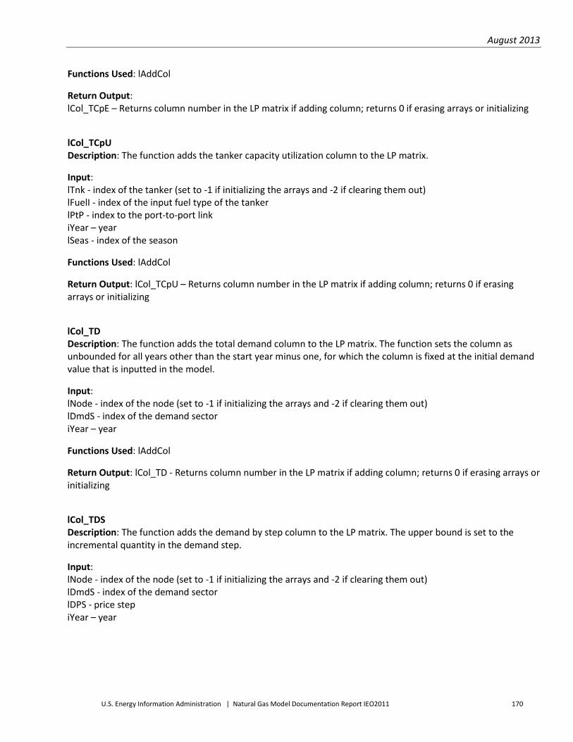
August 2013
U.S. Energy Information Administration | Natural Gas Model Documentation Report IEO2011 170
Functions Used: lAddCol
Return Output: lCol_TCpE – Returns column number in the LP matrix if adding column; returns 0 if erasing arrays or initializing
lCol_TCpU Description: The function adds the tanker capacity utilization column to the LP matrix.
Input: lTnk - index of the tanker (set to -1 if initializing the arrays and -2 if clearing them out) lFuelI - index of the input fuel type of the tanker lPtP - index to the port-to-port link iYear – year lSeas - index of the season
Functions Used: lAddCol
Return Output: lCol_TCpU – Returns column number in the LP matrix if adding column; returns 0 if erasing arrays or initializing
lCol_TD Description: The function adds the total demand column to the LP matrix. The function sets the column as unbounded for all years other than the start year minus one, for which the column is fixed at the initial demand value that is inputted in the model.
Input: lNode - index of the node (set to -1 if initializing the arrays and -2 if clearing them out) lDmdS - index of the demand sector iYear – year
Functions Used: lAddCol
Return Output: lCol_TD - Returns column number in the LP matrix if adding column; returns 0 if erasing arrays or initializing
lCol_TDS Description: The function adds the demand by step column to the LP matrix. The upper bound is set to the incremental quantity in the demand step.
Input: lNode - index of the node (set to -1 if initializing the arrays and -2 if clearing them out) lDmdS - index of the demand sector lDPS - price step iYear – year

August 2013
U.S. Energy Information Administration | Natural Gas Model Documentation Report IEO2011 171
Functions Used: lAddCol
Return Output: lCol_TDS - Returns column number in the LP matrix if adding column; returns 0 if erasing arrays or initializing
Add Row Routines lRow_ACG Description: The function adds the processing asset capacity build constraint (minimum constraint) to the LP matrix if it does not yet exist and sets the right hand side for the constraint.
Input: lNode - index of the node where the processing asset is (set to -1 if initializing the arrays and -2 if clearing them out) lProc - index of the processing asset iYearS - first year of the constraint lPrcRc - index to processing asset constraint
Functions Used: lAddRow
Return Output: lRow_ACG – Returns row number in the LP matrix if adding row; returns 0 if erasing arrays or initializing
lRow_ACL Description: The function adds the processing asset capacity build constraint (maximum constraint) to the LP matrix if it does not yet exist and sets the right hand side for the constraint.
Input: lNode - index of the node where the processing asset is (set to -1 if initializing the arrays and -2 if clearing them out) lProc - index of the processing asset iYearS - first year of the constraint lPrcRc - index to processing asset constraint
Functions Used: None
Return Output: lRow_ACL – Returns row number in the LP matrix if adding row; returns 0 if erasing arrays or initializing
lRow_ACU Description: The function adds the processing asset utilization constraint row to the LP matrix if it does not already exist and sets the right hand side for the constraint.
Input: lNode - index of the node where the processing asset is (set to -1 if initializing the arrays and -2 if clearing them out) lProc - index of the processing asset iYear – year lSeas - index of the season

August 2013
U.S. Energy Information Administration | Natural Gas Model Documentation Report IEO2011 172
Functions Used: lAddRow
Return Output: lRow_ACU – Returns row number in the LP matrix if adding row; returns 0 if erasing arrays or initializing
lRow_ADD Description: The function adds the average daily demand constraint to the LP matrix matrix if it does not yet exist and sets the right hand side for the constraint.
Input: lNode - index of the node (set to -1 if initializing the arrays and -2 if clearing them out) lDmdS - index of the demand sector iYear – year
Functions Used: lAddRow
Return Output: lRow_ADD – Returns row number in the LP matrix if adding row; returns 0 if erasing arrays or initializing
lRow_ARC Description: The function adds the annual resource constraint to the LP matrix if it does not yet exist and sets the right hand side for the constraint.
Input: lNode - index of the node (set to -1 if initializing the arrays and -2 if clearing them out) lSpC - index of the supply category lSPS - supply final price step iYear – year
Functions Used: lAddRow
Return Output: lRow_ARC – Returns row number in the LP matrix if adding row; returns 0 if erasing arrays or initializing
lRow_CC Description: The function adds the regional capital constraint row to the LP matrix if it does not yet exist and sets the right hand side for the constraint.
Input: lReg - index of the region (set to -1 if initializing the arrays and -2 if clearing them out) iYear – year of investment

August 2013
U.S. Energy Information Administration | Natural Gas Model Documentation Report IEO2011 173
Functions Used: lAddRow
Return Output: lRow_CC – Returns row number in the LP matrix if adding row; returns 0 if erasing arrays or initializing
lRow_CI Description: The function adds the regional investment capital constraint row to the LP matrix if it does not yet exist and sets the right hand side for the constraint.
Input: lReg - index of the region (set to -1 if initializing the arrays and -2 if clearing them out) iYear – year of investment
Functions Used: lAddRow
Return Output: lRow_CI – Returns row number in the LP matrix if adding row; returns 0 if erasing arrays or initializing
lRow_CO Description: The function adds the regional other capital constraint row to the LP matrix if it does not yet exist and sets the right hand side for the constraint.
Input: lReg - index of the region (set to -1 if initializing the arrays and -2 if clearing them out) iYear – year
Functions Used: lAddRow
Return Output: lRow_CO – Returns row number in the LP matrix if adding row; returns 0 if erasing arrays or initializing
lRow_EI Description: This function adds the export and import rows to the LP matrix if it does not yet exist and sets the right hand side for the constraint.
Input: lReg - index of the region (set to -1 if initializing the arrays and -2 if clearing them out) iYear – year lSeas - index of the season
Functions Used: lAddRow
Return Output: lRow_EI – Returns row number in the LP matrix if adding row; returns 0 if erasing arrays or initializing

August 2013
U.S. Energy Information Administration | Natural Gas Model Documentation Report IEO2011 174
lRow_EJ Description: This function adds the annual net export constraint rows to the LP matrix if it does not yet exist and sets the right hand side for the constraint.
Input: lReg - index of the region (set to -1 if initializing the arrays and -2 if clearing them out) iYear – year lSeas - index of the season
Functions Used: lAddRow
Return Output: lRow_EI – Returns row number in the LP matrix if adding row; returns 0 if erasing arrays or initializing
lRow_MB Description: The function adds the energy balance row to the LP matrix if it does not yet exist and sets the right hand side for the constraint.
Input: lNode - index of the node (set to -1 if initializing the arrays and -2 if clearing them out) lFuel - index of the fuel type iYear – year lSeas - index of the season
Functions Used: lAddRow
Return Output: lRow_MB – Returns row number in the LP matrix if adding row; returns 0 if erasing arrays or initializing
lRow_PCG Description: The function adds the pipeline asset capacity build constraint (minimum constraint) to the LP matrix if it does not yet exist and sets the right hand side for the constraint.
Input: lPipe - index of the pipline (set to -1 if initializing the arrays and -2 if clearing them out) iYearS - first year of the constraint lPipeC - index to the pipeline constraint
Functions Used: lAddRow
Return Output: lRow_PCG – Returns row number in the LP matrix if adding row; returns 0 if erasing arrays or initializing

August 2013
U.S. Energy Information Administration | Natural Gas Model Documentation Report IEO2011 175
lRow_PCL Description: The function adds the pipeline asset capacity constraint build (maximum constraint) to the LP matrix if it does not yet exist and sets the right hand side for the constraint.
Input: lPipe - index of the pipline (set to -1 if initializing the arrays and -2 if clearing them out) iYearS - first year of the constraint lPipeC - index to the pipeline constraint
Functions Used: lAddRow
Return Output: lRow_PCL – Returns row number in the LP matrix if adding row; returns 0 if erasing arrays or initializing
lRow_PCU Description: This function adds the pipeline asset capacity utilization constraint to the LP matrix if it does not yet exist and sets the right hand side for the constraint.
Input: lPipe - index of the pipeline (set to -1 if initializing the arrays and -2 if clearing them out) iYear – year lSeas - index of the season
Functions Used: lAddRow
Return Output: lRow_PCU – Returns row number in the LP matrix if adding row; returns 0 if erasing arrays or initializing
lRow_PrA Description: The function adds the accelerated production constraint to the LP matrix if it does not yet exist and sets the right hand side for the constraint.
Input: lNode - index of the node (set to -1 if initializing the arrays and -2 if clearing them out) lSpC - index of the supply category lSPS - supply final price step iYear – year lSeas – index of the season
Functions Used: lAddRow
Return Output: lRow_PrA – Returns row number in the LP matrix if adding row; returns 0 if erasing arrays or initializing

August 2013
U.S. Energy Information Administration | Natural Gas Model Documentation Report IEO2011 176
lRow_Prd Description: The function adds the production constraint to the LP matrix if it does not yet exist and sets the right hand side for the constraint.
Input: lNode - index of the node (set to -1 if initializing the arrays and -2 if clearing them out) lSpC - index of the supply category lSPS - supply final price step iYear – year lSeas – index of the season
Functions Used: lAddRow
Return Output: lRow_Prd – Returns row number in the LP matrix if adding row; returns 0 if erasing arrays or initializing
lRow_RSV Description: The function adds the reserves constraint to the LP matrix if it does not yet exist and sets the right hand side for the constraint.
Input: lNode - index of the node (set to -1 if initializing the arrays and -2 if clearing them out) lSpC - index of the supply category lSMS - supply major price step iYear – year
Functions Used: lAddRow
Return Output: lRow_RSV – Returns row number in the LP matrix if adding row; returns 0 if erasing arrays or initializing
lRow_RUR Description: The function adds the remaining undeveloped resources constraint to the LP matrix if it does not yet exist and sets the right hand side for the constraint.
Input: lNode - index of the node (set to -1 if initializing the arrays and -2 if clearing them out) lSpC - index of the supply category lSPS - supply final price step iYear – year
Functions Used: lAddRow
Return Output: lRow_RUR – Returns row number in the LP matrix if adding row; returns 0 if erasing arrays or initializing

August 2013
U.S. Energy Information Administration | Natural Gas Model Documentation Report IEO2011 177
lRow_SCB Description: The function adds the storage asset volume balance constraint to the LP matrix if it does not yet exist and sets the right hand side for the constraint.
Input: lNode - index of the node where the storage asset is (set to -1 if initializing the arrays and -2 if clearing them out) lStor - index of the storage asset iYear - year of the constraint
Functions Used: lAddRow
Return Output: lRow_SCB – Returns row number in the LP matrix if adding row; returns 0 if erasing arrays or initializing
lRow_SCG Description: The function adds the storage asset capacity build constraint (minimum constraint to the LP matrix if it does not yet exist and sets the right hand side for the constraint.
Input: lNode - index of the node where the storage asset is(set to -1 if initializing the arrays and -2 if clearing them out) lStor - index of the storage asset iYearS - first year of the constraint lStrRc - index to storage asset constraint
Functions Used: lAddRow
Return Output: lRow_SCG – Returns row number in the LP matrix if adding row; returns 0 if erasing arrays or initializing
lRow_SCL
Description: The function adds the storage asset capacity build constraint (maximum constraint to the LP matrix if it does not yet exist and sets the right hand side for the constraint.
Input: lNode - index of the node where the storage asset is(set to -1 if initializing the arrays and -2 if clearing them out) lStor - index of the storage asset iYearS - first year of the constraint lStrRc - index to storage asset constraint
Functions Used: lAddRow
Return Output: lRow_SCL – Returns row number in the LP matrix if adding row; returns 0 if erasing arrays or initializing

August 2013
U.S. Energy Information Administration | Natural Gas Model Documentation Report IEO2011 178
lRow_SCU Description: The function adds the storage asset capacity utilization constraint to the LP matrix if it does not yet exist and sets the right hand side for the constraint.
Input: lNode - index of the node where the storage asset is (set to -1 if initializing the arrays and -2 if clearing them out) lStor - index of the storage asset iYear – year lSeas - index of the season
Functions Used: lAddRow
Return Output: lRow_SCU – Returns row number in the LP matrix if adding row; returns 0 if erasing arrays or initializing
lRow_TCG Description: The function adds the tanker asset capacity build constraint (minimum constraint) to the LP matrix if it does not yet exist and sets the right hand side for the constraint.
Input: lTnk - index of the tanker type (set to -1 if initializing the arrays and -2 if clearing them out) iYearS - first year of the constraint lTnkC - index to tanker capacity constraint
Functions Used: lAddRow
Return Output: lRow_TCG – Returns row number in the LP matrix if adding row; returns 0 if erasing arrays or initializing
lRow_TCL Description: The function adds the tanker asset capacity build constraint (maximum constraint) to the LP matrix if it does not yet exist and sets the right hand side for the constraint.
Input: lTnk - index of the tanker type (set to -1 if initializing the arrays and -2 if clearing them out) iYearS - first year of the constraint lTnkC - index to tanker capacity constraint
Functions Used: lAddRow
Return Output: lRow_TCL – Returns row number in the LP matrix if adding row; returns 0 if erasing arrays or initializing
lRow_TCU Description: The function adds the tanker asset capacity utilization constraint to the LP matrix if it does not yet exist and sets the right hand side for the constraint.

August 2013
U.S. Energy Information Administration | Natural Gas Model Documentation Report IEO2011 179
Input: lReg - index of the region where the tanker originates(set to -1 if initializing the arrays and -2 if clearing them out) lTnk - index of the tanker type iYear – year lSeas - index of the season
Functions Used: lAddRow
Return Output: lRow_TCU – Returns row number in the LP matrix if adding row; returns 0 if erasing arrays or initializing
Miscellaneous Functions iFMod Description: The function returns last two digits of a year.
Input: iYear - Year
Functions Used: None
Return Output: Year mod 100
iSaveLPRslts Description: The function copies the results for all variables in the run to the output tables.
Input: iDeleteFlag – Set to true if output tables need to be cleared of all content, false if the data is to be added to the tables.
Functions Used: None
Return Output: iSaveLPRslts – Returns true if there is error in saving results, false otherwise
iUpdate_CapCnsts Description: The function updates the constraints on capacity to reflect capacity decisions that are fixed from the last solution. This is the second to last step in the rolling optimization and prepares the arrays for the next solution period
Input: None
Functions Used: None
Return Output: iUpdate_CapCnsts – Returns true if there is error in updating the constraints and false otherwise

August 2013
U.S. Energy Information Administration | Natural Gas Model Documentation Report IEO2011 180
iUpdate_RsvRes Description: The function updates the reserves and available undiscovered resources to reflect production and reserve additions that are fixed from the last solution. This is the last step in the rolling optimization and prepares the arrays for the next solution period
Input: None
Functions Used: None
Return Output: iUpdate_RsvRes – Returns true if there is error in updating the reserves and resources and false otherwise
Module: mCleanOutputRslts iClean_Output_Tables Description: The function deletes all records from the output tables for a particular run Id. The output tables include all tables that start with tOut.
Input: lRunId_in – The run Id for which all output tables are to be cleared.
Functions Used: None
Return Output: None
Module: mDocument iDocument_Tables Description: The utility function creates a list of all tables and variables in the tables and stores these in the file tZDc_TblDef.
Input: None
Functions Used: None
Return Output: None
iDocument_Queries Description: The utility function creates a list of all queries and their SQL in the database and stores these in the file tZDc_QryDef.
Input: None
Functions Used: None
Return Output: None

August 2013
U.S. Energy Information Administration | Natural Gas Model Documentation Report IEO2011 181
Module: mINGM_Main iINGM_Main Description: This is main function of the INGM model. It calls functions that read data from all the input data files, build the LP matrix, convert it into an MPS file, send it to solver for LP solutions, and finally read and save the LP solution results for a particular run Id.
Input: lRunId_in – Run Id.
Functions Used: iCreateErrorMsg, iRead_Scenario, iRead_All, iGetSolYears, iBuild_Matrix, iBuild_MPS, iRun_CPLEX, iRead_CPLEX, iRun_GAMS, iRead_GAMSRslt, iSaveLPRslts, iOutput_Matrix, iUpdate_CapCnsts, iUpdate_RsvRes, iClear_Matrix
Return Output: None
iRun_CPLEX Description: The function runs the CPLEX program to solve the LP and output the results.
Input: None
Functions Used: None
Return Output: None
iRun_GAMS Description: The function runs the GAMS program to solve the LP and output the results.
Input: None
Functions Used: None
Return Output: None
StripFileAndReturnPath Description: The function strips the file name off of a full DOS path and returns the path less the file name.
Input: FullPath – Full path of the file location (including file name)
Functions Used: None
Return Output: StripFileAndReturnPath – returns the path of the file location without the file name (but includes backslash)
August 2013
U.S. Energy Information Administration | Natural Gas Model Documentation Report IEO2011 182
iGetSolYears Description: The function builds the arrays for the solution periods and mapping of years to solution periods. The start year and input data from tTimeVal provide the initial basis for the solution years but are adjusted to reflect years in the pipeline, processing, storage, or tanker asset constraints.
Input: iSYear - Start year of solution interval iEYear - End year of solution interval (returned as global variable value)
Functions Used: None
Return Output: None
Module: mLPSetUp
Initialization/Clearing Routines
iInitializeLP Description: The function initializes all the LP matrix arrays by dimensioning them and setting the number of rows, columns, and coefficients to be empty.
Input: lEstRow - estimate of the number of rows lEstCol - estimate of the number of columns fDens - estimated density of the matrix (number of coefficients per column on average)
Functions Used: None
Return Output: iInitializeLP – Returns 0 if there is no error in execution of the function.
iClearLP Description: The function clears data from all the LP matrix arrays, resets the last row, column, and coefficient; and erases the arrays.
Input: None
Functions Used: None
Return Output: iClearLP – Returns 0 if there is no error in execution of the function.

August 2013
U.S. Energy Information Administration | Natural Gas Model Documentation Report IEO2011 183
Matrix Building lAddRow Description: The function adds a row to the LP matrix and stores the right hand side as the coefficient in column zero. It saves the name, type, and right hand side of the row. The type indicates if it is less than or equal to, greater than or equal to, equal to, and unconstrained. This routine returns the row number.
Input: sName – Name of the row in the LP matrix sSense – Sense of the constraint (row) in the LP matrix; -1(<=), 1(>=), 0(=), -2(N) fRHS – RHS value of the constraint
Functions Used: iAddCoef
Return Output: lAddRow – Row number in the LP matrix
lAddCol
Description: The function adds a column to the LP matrix. It saves the name and lower and upper bounds. It returns the column number.
Input: sName – Name of the column in the LP matrix fMin – Minimum value the column (variable) can take fMax – Maximum value the column (variable) can take
Functions Used: None
Return Output: lAddCol – Column number in the LP matrix
iAddCoef Description: The function adds a coefficient to a particular row and column in the LP matrix.
Input: lRow - Index of the row lCol - Index of the column fVal - Coefficient value Functions Used: None
Return Output: iAddCoef – Returns 0 if there is no error in execution of the function.

August 2013
U.S. Energy Information Administration | Natural Gas Model Documentation Report IEO2011 184
Debugging iTestCoef Description: This is a debugging routine which checks the LP matrix for duplicate entries of coefficients. It is not currently used.
Input: None
Functions Used: None
Return Output: iTestCoef – Returns true value if there is a duplicate co-efficient, false otherwise
iTest_Rows Description: This is a debugging routine which checks the LP matrix to make sure there are no duplicate row names. It is not currently used.
Input: None
Functions Used: None
Return Output: iTest_Rows – Returns true value if there is a duplicate row name, false otherwise
iTest_Cols
Description: This a debugging routine which checks the LP matrix to make sure there are no duplicate column names. It is not currently used.
Input: None
Functions Used: None
Return Output: iTest_Cols – Returns true value if there is a duplicate row name, false otherwise
iOutput_Matrix Description: The function clears all data from three arrays tMatrix_Rows, tMatrix_Cols, and tMatrix_Coef and then populates them with the LP matrix and output data from the LP run. The arrays store slack and dual values of variables amongst other details. Input: None
Functions Used: None
Return Output: None

August 2013
U.S. Energy Information Administration | Natural Gas Model Documentation Report IEO2011 185
MPS File Generation iBuild_MPS Description: The function builds the MPS file using coefficient values, RHS values, and bound values from the LP matrix. The function converts all values used in the MPS file to a fixed length of 12 characters using sub-function fxLen.
Input: None
Functions Used: fxLen
Return Output: None
fxLen Description: The function converts the coefficient value into a fixed length string of 12 characters including the decimal point.
Input: sTextIn – Coefficient value as a string
Functions Used: None
Return Output: fxLen – Returns the coefficient value in fixed length
Module: mOutputQueries This module contains the routines which build the queries used for the output processing.
iGet_DmdQuery Description: The function builds the SQL for the demand graphs and reports
Input:
• iAgg - regional aggregation (0 - global, 1-regional, 2-nodal) • iSea - true if seasonal data required • iSec - true if sector data required • sSQLO - output SQL string for spreadsheets • sSQLT - output SQL string for graphs • sHdr - Header for the graph • sUnit - Units for the graph
Functions Used: None
Return Output: None

August 2013
U.S. Energy Information Administration | Natural Gas Model Documentation Report IEO2011 186
iGet_EOYRsvQuery Description: The function builds the SQL for the EOY reserves graphs and reports
Input:
• iAgg - regional aggregation (0 - global, 1-regional, 2-nodal) • iSea - true if seasonal data required • iSec - true if sector (category) data required • sSQLO - output SQL string for spreadsheets • sSQLT - output SQL string for graphs • sHdr - Header for the graph • sUnit - Units for the graph
Functions Used: None
Return Output: None
iGet_RemResQuery Description: The function builds the SQL for the EOY remaining undevelop resources graphs and reports.
Input:
• iAgg - regional aggregation (0 - global, 1-regional, 2-nodal) • iSea - true if seasonal data required • iSec - true if sector (category) data required • sSQLO - output SQL string for spreadsheets • sSQLT - output SQL string for graphs • sHdr - Header for the graph • sUnit - Units for the graph
Functions Used: None
Return Output: None
iGet_RsvAddQuery Description: The function builds the SQL for the annual reserve additions graphs and reports.
Input:
• iAgg - regional aggregation (0 - global, 1-regional, 2-nodal) • iSea - true if seasonal data required • iSec - true if sector (category) data required • sSQLO - output SQL string for spreadsheets • sSQLT - output SQL string for graphs • sHdr - Header for the graph • sUnit - Units for the graph

August 2013
U.S. Energy Information Administration | Natural Gas Model Documentation Report IEO2011 187
Functions Used: None
Return Output: None
iGet_ProdQuery Description: The function builds the SQL for the annual production graphs and reports.
Input:
• iAgg - regional aggregation (0 - global, 1-regional, 2-nodal) • iSea - true if seasonal data required • iSec - true if sector (category) data required • sSQLO - output SQL string for spreadsheets • sSQLT - output SQL string for graphs • sHdr - Header for the graph • sUnit - Units for the graph
Functions Used: None
Return Output: None
iGet_AccProdQuery Description: The function builds the SQL for the annual accelerated production graphs and reports.
Input:
• iAgg - regional aggregation (0 - global, 1-regional, 2-nodal) • iSea - true if seasonal data required • iSec - true if sector (category) data required • sSQLO - output SQL string for spreadsheets • sSQLT - output SQL string for graphs • sHdr - Header for the graph • sUnit - Units for the graph
Functions Used: None
Return Output: None
August 2013
U.S. Energy Information Administration | Natural Gas Model Documentation Report IEO2011 188
iGet_NCFQuery Description: The function builds the SQL for the annual net cash flow graphs and reports.
Input:
• iAgg - regional aggregation (0 - global, 1-regional, 2-nodal) • iSea - true if seasonal data required • iSec - true if sector data required • sSQLO - output SQL string for spreadsheets • sSQLT - output SQL string for graphs • sHdr - Header for the graph • sUnit - Units for the graph
Functions Used: None
Return Output: None
iGet_OFuelQuery Description: The function builds the SQL for the annual other fuel demand graphs and reports.
Input:
• iAgg - regional aggregation (0 - global, 1-regional, 2-nodal) • iSea - true if seasonal data required • iSec - true if sector (category) data required • sSQLO - output SQL string for spreadsheets • sSQLT - output SQL string for graphs • sHdr - Header for the graph • sUnit - Units for the graph
Functions Used: None
Return Output: None
iGet_PricesQuery Description: The function builds the SQL for the annual or seasonal price graphs and reports.
Input:
• iAgg - regional aggregation (0 - global, 1-regional, 2-nodal) • iSea - true if seasonal data required • iSec - true if sector (category) data required • sSQLO - output SQL string for spreadsheets • sSQLT - output SQL string for graphs • sHdr - Header for the graph • sUnit - Units for the graph

August 2013
U.S. Energy Information Administration | Natural Gas Model Documentation Report IEO2011 189
Functions Used: None
Return Output: None
iGet_PipeCQuery Description: The function builds the SQL for the annual pipeline capacity graphs and reports.
Input:
• iAgg - regional aggregation (0 - global, 1-regional, 2-nodal) • iSea - true if seasonal data required • iSec - true if sector (category) data required • sSQLO - output SQL string for spreadsheets • sSQLT - output SQL string for graphs • sHdr - Header for the graph • sUnit - Units for the graph
Functions Used: None
Return Output: None
iGet_PipeUtlQuery Description: The function builds the SQL for the annual and seasonal pipeline utilization graphs and reports.
Input:
• iAgg - regional aggregation (0 - global, 1-regional, 2-nodal) • iSea - true if seasonal data required • iSec - true if sector (category) data required • sSQLO - output SQL string for spreadsheets • sSQLT - output SQL string for graphs • sHdr - Header for the graph • sUnit - Units for the graph
Functions Used: None
Return Output: None

August 2013
U.S. Energy Information Administration | Natural Gas Model Documentation Report IEO2011 190
iGet_StorCQuery Description: The function builds the SQL for the annual storage capacity graphs and reports.
Input:
• iAgg - regional aggregation (0 - global, 1-regional, 2-nodal) • iSea - true if seasonal data required • iSec - true if sector (category) data required • sSQLO - output SQL string for spreadsheets • sSQLT - output SQL string for graphs • sHdr - Header for the graph • sUnit - Units for the graph
Functions Used: None
Return Output: None
iGet_StorUtlQuery Description: The function builds the SQL for the annual and seasonal storage utilization graphs and reports.
Input:
• iAgg - regional aggregation (0 - global, 1-regional, 2-nodal) • iSea - true if seasonal data required • iSec - true if sector (category) data required • sSQLO - output SQL string for spreadsheets • sSQLT - output SQL string for graphs • sHdr - Header for the graph • sUnit - Units for the graph
Functions Used: None
Return Output: None
iGet_ProcCQuery Description: The function builds the SQL for the annual processing asset capacity graphs and reports.
Input:
• iAgg - regional aggregation (0 - global, 1-regional, 2-nodal) • iSea - true if seasonal data required • iSec - true if sector (category) data required • sSQLO - output SQL string for spreadsheets • sSQLT - output SQL string for graphs • sHdr - Header for the graph • sUnit - Units for the graph

August 2013
U.S. Energy Information Administration | Natural Gas Model Documentation Report IEO2011 191
Functions Used: None
Return Output: None
iGet_ProcUtlQuery Description: The function builds the SQL for the annual and seasonal procssing asset utilization graphs and reports.
Input:
• iAgg - regional aggregation (0 - global, 1-regional, 2-nodal) • iSea - true if seasonal data required • iSec - true if sector (category) data required • sSQLO - output SQL string for spreadsheets • sSQLT - output SQL string for graphs • sHdr - Header for the graph • sUnit - Units for the graph
Functions Used: None
Return Output: None
iGet_TnkCQuery Description: The function builds the SQL for the annual tanker asset capacity graphs and reports.
Input:
• iAgg - regional aggregation (0 - global, 1-regional, 2-nodal) • iSea - true if seasonal data required • iSec - true if sector (category) data required • sSQLO - output SQL string for spreadsheets • sSQLT - output SQL string for graphs • sHdr - Header for the graph • sUnit - Units for the graph
Functions Used: None
Return Output: None
iGet_TnkUtlQuery Description: The function builds the SQL for the annual and seasonal tanker utilization graphs and reports.
August 2013
U.S. Energy Information Administration | Natural Gas Model Documentation Report IEO2011 192
Input:
• iAgg - regional aggregation (0 - global, 1-regional, 2-nodal) • iSea - true if seasonal data required • iSec - true if sector (category) data required • sSQLO - output SQL string for spreadsheets • sSQLT - output SQL string for graphs • sHdr - Header for the graph • sUnit - Units for the graph
Functions Used: None
Return Output: None
iGet_ReInjQuery Description: The function builds the SQL for the annual and seasonal gas reinjection graphs and reports.
Input:
• iAgg - regional aggregation (0 - global, 1-regional, 2-nodal) • iSea - true if seasonal data required • iSec - true if sector (category) data required • sSQLO - output SQL string for spreadsheets • sSQLT - output SQL string for graphs • sHdr - Header for the graph • sUnit - Units for the graph
Functions Used: None
Return Output: None
Module: mReadData
Main Controlling Routine iRead_All Description: Uses multiple functions to either input the data from the regions or clear out data from all arrays that contain input data.
Input: iRead - the argument is set to True if the arrays should be initialized and the data read, and False if the arrays should be freed up.
Functions Used: iRead_DmdSectors, iRead_Fuels, iRead_Regions, iRead_ImpExpCnstr, iRead_Seasons, iRead_SupCat, iRead_Nodes, iRead_DmdBase, iRead_DmdBPrc, iRead_DmdNdeAlloc, iRead_DmdSeasAlloc, iRead_OthDmd, iRead_PipeAsset, iRead_PipeCnst, iRead_PorttoPort, iRead_ProcAssetType, iRead_ProcAsset, iRead_ProcAssetFuel, iRead_ProcRCnst, iRead_StorAsset, iRead_StorRCnst, iRead_SupplyBase, iRead_TankerAsset, iRead_TankerCnst, iRead_TankerFuel, iRead_TankerPort, iRead_TimeVal, iRead_PScalar

August 2013
U.S. Energy Information Administration | Natural Gas Model Documentation Report IEO2011 193
Return Output: Returns a 0 if all processing completed normally and -1 if an error occurred.
Routines For Each Input Table iRead_DmdBase Description: The function reads demand data by node from tDmdBase and copies the data into arrays. Returns error if gaps exist in data. The function calculates the demand for all years that data has not been provided. It calculates the growth rate from the last ten years that data is available and determines the demand for all subsequent years for which data is not available using the calculated growth rate. The function finally ensures that there is a demand value either inputted or calculated for each year in the run.
Input: iRead - the argument is set to True if the arrays should be initialized and the data read, and False if the arrays should be freed up.
Functions Used: lGetId, iCreateErrorMsg
Return Output: iRead_DmdBase - Returns -1 if error exists, otherwise set to 0
iRead_DmdSeasAlloc Description: The function reads seasonal share (allocation) of demand by node and sector from tDmdSeasAlloc and copies the data into arrays. The function ensures that the seasonal factors add up to one for each season.
Input: iRead - the argument is set to True if the arrays should be initialized and the data read, and False if the arrays should be freed up.
Functions Used: lGetId, iCreateErrorMsg
Return Output: iRead_DmdSeasAlloc - Returns -1 if error exists, otherwise set to 0
iRead_DmdSectors Description: The function ensures that Demand Sector specifications exist in tDmdSectors and copies the data into arrays. Returns error if data does not exist. The function also clears data from all arrays as an option.
Input: iRead - the argument is set to True if the arrays should be initialized and the data read, and False if the arrays should be freed up.
Functions Used: iCreateErrorMsg
Return Output: iRead_DmdSectors - Returns -1 if error exists, otherwise set to 0.
iRead_Fuels
Description: The function ensures that Fuel Specifications exist in tFuel and then copies the data into arrays depending upon whether the data is either for demand or supply. Returns error if data does not exist. The function also clears data from all arrays as an option.
Input: iRead - the argument is set to True if the arrays should be initialized and the data read, and False if the arrays should be freed up.

August 2013
U.S. Energy Information Administration | Natural Gas Model Documentation Report IEO2011 194
Functions Used: iCreateErrorMsg
Return Output: iRead_Fuels - Returns -1 if error exists, otherwise set to 0.
iRead_ImpExpCnstr Description: The function reads all import/export constraints from tImpExt_Cnstr and copies the data into arrays. The function converts any NULL values for import constraint, export constraint, or investment constraint into value “-99.” The function also returns an error if the Fuel id is missing.
Input: iRead - the argument is set to True if the arrays should be initialized and the data read, and False if the arrays should be freed up.
Functions Used: lGetId, iCreateErrorMsg
Return Output: iRead_ImpExpCnstr - Returns -1 if error exists, otherwise set to 0
iRead_Nodes Description: The function ensures that nodal specifications exist in tNode and copies the data into arrays. Returns error if data does not exist. The function also ensures that the region id specified for each of the nodes exists in the list of regions specified for the run.
Input: iRead - the argument is set to True if the arrays should be initialized and the data read, and False if the arrays should be freed up.
Functions Used: lGetId, iCreateErrorMsg
Return Output: iRead_Nodes - Returns -1 if error exists, otherwise set to 0
iRead_OthDmd Description: The function reads non-natural gas fuel prices from tOthDmd and copies the data into arrays. The function returns an error if the Fuel id is either NULL or is not being used in the current run.
Input: iRead - the argument is set to True if the arrays should be initialized and the data read, and False if the arrays should be freed up.
Functions Used: lGetId, iCreateErrorMsg
Return Output: iRead_OthDmd - Returns -1 if error exists, otherwise set to 0
iRead_PipeAsset Description: The function reads pipeline asset details from tPipelineAsset and copies the data into arrays. The function ensures that each pipeline asset has a fuel id, origin id, and destination id, returning an error in case any one is missing.
Input: iRead - the argument is set to True if the arrays should be initialized and the data read, and False if the arrays should be freed up.

August 2013
U.S. Energy Information Administration | Natural Gas Model Documentation Report IEO2011 195
Functions Used: iCreateErrorMsg
Return Output: iRead_PipeAsset - Returns -1 if error exists, otherwise set to 0
iRead_PipeCnst Description: The function reads all pipeline constraint data from tPipelineAsset_Cnstr and copies the data into arrays. The function ensures that the pipeline id is included in the list of pipeline ids for the run, that the first year of the constraint is earlier than the last year, and that the minimum capacity of the pipeline is less than the maximum capacity. The function also checks for overlapping constraints.
iRead - the argument is set to True if the arrays should be initialized and the data read, and False if the arrays should be freed up.
Functions Used: lGetId, iCreateErrorMsg
Return Output: iRead_PipeCnst - Returns -1 if error exists, otherwise set to 0
iRead_PorttoPort Description: The function reads all port to port specifications from tPorttoPort and copies the data into arrays. The function also ensures that there is an origin and destination node for each port-to-port id.
iRead - the argument is set to True if the arrays should be initialized and the data read, and False if the arrays should be freed up.
Functions Used: lGetId, iCreateErrorMsg
Return Output: iRead_PorttoPort - Returns -1 if error exists, otherwise set to 0
iRead_ProcAsset Description: The function reads all processing asset specifications from tProcessingAsset and copies the data into arrays.
iRead - the argument is set to True if the arrays should be initialized and the data read, and False if the arrays should be freed up.
Functions Used: iCreateErrorMsg
Return Output: iRead_ProcAsset - Returns -1 if error exists, otherwise set to 0
iRead_ProcAssetType Description: The function ensures that all processing asset types are available in tProcessingAsset_Type and copies the data into arrays. Returns error if data does not exist.
iRead - the argument is set to True if the arrays should be initialized and the data read, and False if the arrays should be freed up.

August 2013
U.S. Energy Information Administration | Natural Gas Model Documentation Report IEO2011 196
Functions Used: iCreateErrorMsg
Return Output: iRead_ProcAssetType - Returns -1 if error exists, otherwise set to 0
iRead_ProcAssetFuel Description: The function reads all fuel specifications for each processing asset from tProcessingAsset_Fuel and copies the data into arrays. The function ensures that Asset id and Fuel id used in the database correspond to those used in the run.
iRead - the argument is set to True if the arrays should be initialized and the data read, and False if the arrays should be freed up.
Functions Used: iCreateErrorMsg
Return Output: iRead_ProcAssetFuel - Returns -1 if error exists, otherwise set to 0
iRead_ProcRCnst Description: The function reads all regional constraints for each processing asset from tProcessingAsset_RegCnstr and copies the data into arrays. The function ensures that the asset id and node id are included, that the first year of the constraint is earlier than the last year, and that the minimum capacity of the asset is less than the maximum capacity. The function sets the start year for all assets. It also checks for overlapping constraints.
Input: iRead - the argument is set to True if the arrays should be initialized and the data read, and False if the arrays should be freed up.
Functions Used: lGetId, iCreateErrorMsg
Return Output: iRead_ProcRCnst - Returns -1 if error exists, otherwise set to 0
iRead_PScalar Description: The function reads the price scalar data for five asset types by year and sets up the regional price discount arrays to account for regional differences in discount rates.
Input: iRead - the argument is set to True if the arrays should be initialized and the data read, and False if the arrays should be freed up.
Functions Used: iCreateErrorMsg
Return Output:iRead_PScalar - Returns -1 if error exists, otherwise set to 0

August 2013
U.S. Energy Information Administration | Natural Gas Model Documentation Report IEO2011 197
iRead_Regions Description: The function ensures that regional specifications exist in tRegion and copies the data into arrays. Returns error if data does not exist. The function converts any NULL values for demand base price adjustment into zero values. The function also clears data from all arrays as an option.
Input: iRead - the argument is set to True if the arrays should be initialized and the data read, and False if the arrays should be freed up.
Functions Used: iCreateErrorMsg
Return Output: iRead_Regions - Returns -1 if error exists, otherwise set to 0
iRead_Seasons Description: The function ensures that seasonal specifications exist in tSeason and copies the data into arrays. Returns error if data does not exist. The function also ensures that the total number of days in the different seasons add up to 365, and if not returns an error.
Input: iRead - the argument is set to True if the arrays should be initialized and the data read, and False if the arrays should be freed up.
Functions Used: lGetId, iCreateErrorMsg
Return Output: iRead_Seasons - Returns -1 if error exists, otherwise set to 0
iRead_StorAsset Description: The function reads all storage asset specifications from tStorageAsset and copies the data into arrays.
Input: iRead - the argument is set to True if the arrays should be initialized and the data read, and False if the arrays should be freed up.
Functions Used: iCreateErrorMsg
Return Output: iRead_StorAsset - Returns -1 if error exists, otherwise set to 0
iRead_StorRCnst Description: The function reads all storage asset constraints from tStorageAsset_RegCnstr and copies the data into arrays. The function ensures that the storage id and node id are included, that the first year of the constraint is earlier than the last year, and that the minimum capacity of the asset is less than the maximum capacity. The function sets the start year for all storage assets. It also checks for overlapping constraints.
Input: iRead - the argument is set to True if the arrays should be initialized and the data read, and False if the arrays should be freed up.
Functions Used: lGetId, iCreateErrorMsg

August 2013
U.S. Energy Information Administration | Natural Gas Model Documentation Report IEO2011 198
Return Output: iRead_StorRCnst - Returns -1 if error exists, otherwise set to 0
iRead_SupplyBase Description: The function reads all supply base specifications from tSupplyBase and copies the data into arrays. The function ensures that the supply category id and node id are included and the minimum development costs at which reserves come online is less than the maximum development costs.
Input: iRead - the argument is set to True if the arrays should be initialized and the data read, and False if the arrays should be freed up.
Functions Used: lGetId, iCreateErrorMsg
Return Output: iRead_SupplyBase - Returns -1 if error exists, otherwise set to 0
iRead_SupCat Description: The function ensures that supply category details exist in tSupplyCat and copies the data into arrays. Returns error if data does not exist.
Input: iRead - the argument is set to True if the arrays should be initialized and the data read, and False if the arrays should be freed up.
Functions Used: iCreateErrorMsg
Return Output: iRead_SupCat - Returns -1 if error exists, otherwise set to 0
iRead_TankerAsset Description: The function reads all tanker asset specifications from tTankerAsset and copies the data into arrays.
Input: iRead - the argument is set to True if the arrays should be initialized and the data read, and False if the arrays should be freed up.
Functions Used: iCreateErrorMsg
Return Output: iRead_TankerAsset - Returns -1 if error exists, otherwise set to 0
iRead_TankerCnst Description: The function reads all tanker constraints from tTankerAsset_Cnstr and copies the data into arrays. The function ensures that the tanker id is available, that the first year of the constraint is earlier than the last year, and that the minimum capacity of the tanker is less than the maximum capacity. The function sets the start year for all storage assets. It also checks for overlapping constraints.
Input: iRead - the argument is set to True if the arrays should be initialized and the data read, and False if the arrays should be freed up.

August 2013
U.S. Energy Information Administration | Natural Gas Model Documentation Report IEO2011 199
Functions Used: lGetId, iCreateErrorMsg
Return Output: iRead_TankerCnst - Returns -1 if error exists, otherwise set to 0
iRead_TankerFuel Description: The function reads all tanker input and output fuel data from tTankerFuel and copies the data into arrays. The function ensures that tanker id, input fuel id, and output fuel id are available.
Input: iRead - the argument is set to True if the arrays should be initialized and the data read, and False if the arrays should be freed up.
Functions Used: lGetId, iCreateErrorMsg
Return Output: iRead_TankerFuel - Returns -1 if error exists, otherwise set to 0
iRead_TankerPort Description: The function reads all tanker port details from tTankerPort and copies the data into arrays. The function ensures that tanker id and node id are available.
Input: iRead - the argument is set to True if the arrays should be initialized and the data read, and False if the arrays should be freed up.
Functions Used: lGetId, iCreateErrorMsg
Return Output: iRead_TankerPort - Returns -1 if error exists, otherwise set to 0
iRead_Scenario Description: The function reads the scenario specifications for the selected scenario.
Input: lRunId – the ID of the scenario.
Functions Used: iCreateErrorMsg
Return Output: iRead_Scenario - Returns -1 if error exists, otherwise set to 0
iRead_TimeVal Description: The function reads all time step details from tTimeStep and copies the data into arrays. The function ensures that tanker id and node id are available.
Input: iRead - the argument is set to True if the arrays should be initialized and the data read, and False if the arrays should be freed up.
Functions Used: lGetId, iCreateErrorMsg
Return Output: iRead_TimeVal - Returns -1 if error exists, otherwise set to 0

August 2013
U.S. Energy Information Administration | Natural Gas Model Documentation Report IEO2011 200
Miscellaneous Routines
lGetId Description: This function is a generic function used to match an ID from the database to the index of the value in arrays used to store the data. If it cannot find the ID then an error code is returned otherwise the index in the array is returned.
Input: lIdT – Represents either a Demand Sector or Region id lId – Represents a array with a list of all the Demand Sector or Region ids. lNId – The value represents the number of Demand Sectors or Regions
Functions Used: None
Return Output: lGetId - Returns -1 if error exists, otherwise set to the index in the array that matches the ID.
iCreateErrorMsg Description: This routine either stores an error message in the error log or deletes an already existing error message by run id.
Input: iType - This is the type of call which is set to -1 to initialize and 0 to add error message lErr – This is the Error Id sMsg – This is the description of the Error in text
Functions Used: None
Return Output: iCreateErrorMsg - Argument set to -1 if error exists, otherwise set to 0.
Module: mReadMPSRslt iRead_CPLEX Description: This function reads in the CPLEX output file and stores the LP results for the rows and columns in the row and column output arrays
Input: None
Functions Used: None
Return Output: None

August 2013
U.S. Energy Information Administration | Natural Gas Model Documentation Report IEO2011 201
iRead_GAMSRslt Description: This function reads in the GAMS output file and stores the LP results for the rows and columns in the row and column output arrays
Input: None
Functions Used: None
Return Output: None
Module: mRefIntegrity This module contains ancillary programs to identify areas in the database that do not meet referential integrity rules.
iTest Description: This function controls the evaluation by scenario for node, region, fuel, and season.
Input: None
Functions Used: iRefInt_FuelId, iRefInt_NodeId, iRefInt_RegionId, iRefInt_SeasonId
Return Output: None
iRefInt_FuelId Description: This function tests the referential integrity of the FuelId.
Input: None
Functions Used: iCreateErrorMsg
Return Output: None
iRefInt_NodeId Description: This function tests the referential integrity of the NodeId.
Input: None
Functions Used: iCreateErrorMsg
Return Output: None
iRefInt_RegionId Description: This function tests the referential integrity of the RegionId.
Input: None

August 2013
U.S. Energy Information Administration | Natural Gas Model Documentation Report IEO2011 202
Functions Used: iCreateErrorMsg
Return Output: None
iRefInt_SeasonId Description: This function tests the referential integrity of the SeasonId.
Input: None
Functions Used: iCreateErrorMsg
Return Output: None
Module: mShellWait ShellWait:
Notice: This code was originally written by Terry Kreft. It is not to be altered or distributed, except as part of an application. You are free to use it in any application, provided the copyright notice is left unchanged.
Description: The subroutine starts an external routine and waits for it to complete.
Input: PathName: Full command line of application to run WindowStyle: Set to 1
Functions Used: None
Return Output: None
Miscellaneous Queries Query Description Units
qClean_Matrix_Coef Deletes all rows from the debug
matrix output data for coefficients
qClean_Matrix_Col Deletes all rows from the debug
matrix output data for columns
qClean_Matrix_Row Deletes all rows from the debug
matrix output data for rows
qTest_Rowcol Debug query to review LP
August 2013
U.S. Energy Information Administration | Natural Gas Model Documentation Report IEO2011 203
Appendix E. References 1. Tobin, J. et al, “Natural Gas Processing: The Crucial Link Between Natural Gas Production and Its
Transportation to Market,” Energy Information Administration, Office of Oil and Gas, January 2006, available on the web at http://www.eia.gov/pub/oil_gas/natural_gas/feature_articles/2006/ngprocess/ngprocess.pdf
2. “The Global Liquefied Natural Gas Market: Status and Outlook,” Energy Information Administration, Office of Oil and Gas, December 2003, available on the web at http://www.eia.gov/oiaf/analysispaper/global/lngindustry.html
3. Available on the web at http://www.findarticles.com/p/articles/mi_m0EIN/is_2005_Oct_19/ai_n15723999 4. Bipin P., “Gas Monetisation: A Techno-Economic Comparison Of Gas-To-Liquid and LNG,” 7th World
Congress of Chemical Engineering, Glasgow 2005, available on the web at https://www.fwc.com/publications/tech_papers/files/IChemE%20WCCE%2005%20LNG%20versus%20GTL.pdf
5. Phang, C., “CostInfoV2.xls,” Energy Information Administration, provided on May 31, 2006 6. “Tables of liquefaction plant,” LNG Journal, October 2007: 41-42. 7. “Tables of reception terminals,” LNG Journal October 2007: 38-41 8. Cochener, J., “GTL Technology Appendix,” Energy Information Administration OIAF: Synfuels Technology
Review (A primer on Fischer-Tropsch derived fuels covering BTL, CTL, and GTL) , Draft, updated November 3, 2005
9. “GTL: Prospects for Development’, Panorama 2006, available on the web at http://www.ifp.com/information-publications/notes-de-synthese-panorama/panorama-2006/le-gtl-perspectives-et-developpement
10. Available on the web at http://www.greencarcongress.com/2006/06/oryx_gtl_opens_.html 11. Available on the web at http://www.energypulse.net/centers/article/article_display.cfm?a_id=1087 12. Available on the web at http://www.shipbuildinghistory.com/ 13. Available on the web at http://www.mol.co.jp/ir-e/library/pdf/ar-e2006.pdf 14. Available on the web at http://www.bea.gov/national/xls/gdplev.xls, data downloaded on 10/28/2005. 15. J. Cho et al, “Large LNG Carrier poses economic advantages, technical challenges,” LNG Observer, October 3,
2005, available on the web at http://www.ogj.com/index/search.html?si=ogj+&collection=ogj&keywords=Large+LNG+Carrier+poses+economic+advantages%2C+technical+challenges%92
16. Available on the web at http://www.world-register.org/ 17. Available on the web at http://www.lethagencies.com/calculator.asp?Port=SUEZTREG 18. Available on the web at http://www.pancanal.com/common/general/reports/informe-anual-2005.pdf 19. Tobin, J., “U.S.A.: State to State border capacities of pipelines - ‘STBORDER .xls’,” Energy Information
Administration, May 23, 2006 20. Gas Infrastructure Europe (GIE), “The European Natural Gas Network and capacities at cross-border points in
the primary market,”, available on the web at http://www.gie.eu.com/download/gridmap/GTE_070sml.pdf 21. “Gazprom in Figures 2001-2005,” available on the web at
http://old.gazprom.ru/documents/Statistika_Eng_2001-2005.pdf 22. Provided by Energy Information Administration, March 31, 2006 23. “Construc8.xls,” Energy Information Administration, August 5, 2006 24. “Listing on international pipeline projects: ‘Pipelines.xls’,” Energy Information Administration, March 31,
2006 25. Smith, E., C., “US Gas Carriers' 2005 Net Incomes Climb; Construction Costs Plummet,” Oil & Gas Journal,
September 11, 2006, Vol. 104.34.

August 2013
U.S. Energy Information Administration | Natural Gas Model Documentation Report IEO2011 204
26. Rockies Express Project, “Fuel Guidance”, available on the web at http://www.kindermorgan.com/business/gas_pipelines/rockies_express/
27. Lecarpentier, A., "Underground Gas Storage in the World: Serving Market Needs,” CEDIGAZ, June 2006 28. “Activities of Underground Natural Gas Storage Operators, by State,” Energy Information Administration,
August 2006 and August 2007, availble on the web at http://www.eia.gov/pub/oil_gas/natural_gas/data_publications/natural_gas_monthly/current/pdf/table_12.pdf
29. “More underground storage for increased gas consumption,” United Nations Economic Commission For Europe (UNECE), Press Release ECE/ENE/00/1, Geneva, 15 February 2000
30. “Natural Gas Information 2005 Report,” International Energy Agency 31. “GSE Storage Investment Database,” November 2007, available on the web at
http://www.gie.eu.com/gse/storageprojects/downloads/20070706_GSE Storage Projects Database_FINAL.xls
32. “Natural Gas Consumption by End Use”, Energy Information Administration Natural Gas Navigator, available on the web at http://www.eia.doe.gov/dnav/ng/ng_cons_sum_a_EPG0_VC0_mmcf_a.htm
33. “Energy Statistics Handbook: Natural Gas,” Statistics Canada, available on the web at http://www.statcan.ca/english/freepub/57-601-XIE/57-601-XIE2007001.pdf
34. "Status of LNG Projects in Mexico," available on the web at http://www.rrc.state.tx.us/commissioners/carrillo/mexico/2006/LNG__DR__BRENA.pdf
35. Census Data 2001, Census of India, available on the web at http://www.censusindia.gov.in/Census_Data_2001/Census_Data_Online/Population/Total_Population.aspx?cki=fhUodZ1vHFd
36. “Long-Term Energy Demand and Supply Outlook for the 31 Provinces in China through 2030,” Institute of Energy Economics, Japan (IEEJ), pg. 40, available on the web at http://eneken.ieej.or.jp/en/data/pdf/353.pdf
37. Available on the web at http://www.gazprom.com/f/posts/88/439833/1report_eng.pdf 38. “Consumption by End Use,” Energy Information Administration Natural Gas Navigator, available on the web
at http://www.eia.gov/dnav/ng/ng_cons_sum_dcu_nus_m.htm 39. Electricity Generated and Purchased Bulletin, available on the web at
http://www.fepc.or.jp/english/news/generated_purchased/2005.html 40. Monthly Energy Statistics, available on the web at http://www.keei.re.kr/main.nsf/index_en.html 41. Natural Gas Supply and Consutpsion, Eurostat, available on the web at
http://nui.epp.eurostat.ec.europa.eu/nui/show.do?dataset=nrg_103a&lang=en 42. ”Conventional Oil and Gas Resources,” The United States Geological Survey (USGS) National Assessment of
Oil and Gas Resources Update, November 2005, available on the web at http://energy.cr.usgs.gov/oilgas/noga/index.htm
43. “Assessment of Undiscovered Technically Recoverable Oil and Gas Resources of the Nation’s Outer Continental Shelf,” Mineral Management Services The U.S. Offshore Federal Resources, 2006
44. The USGS, World Petroleum Assessment, 2000, available on the web at http://pubs.usgs.gov/dds/dds-060/assmap.html
45. “Balancing Natural Gas Policy – Fueling the Demands of a Growing Economy,” National Petroleum Council, Washington, D.C., 2003
46. “Reserves at December 31, 2006,” 2007 Canadian Association of Petroleum Producers (CAPP) 47. “Worldwide Look at Reserves and Production-Worldwide Production,” Oil & Gas Journal Subscriber Surveys,
December 24, 2007. 48. Historical Statistical Data 1965-2008, BP Statistical Review of World Energy, available on the web at
http://www.bp.com/liveassets/bp_internet/globalbp/globalbp_uk_english/reports_and_publications/statistical_energy_review_2008/STAGING/local_assets/2009_downloads/statistical_review_of_world_energy_full_report_2009.xls#'Gas - Proved reserves history '!A1
August 2013
U.S. Energy Information Administration | Natural Gas Model Documentation Report IEO2011 205
49. Holditch, S., A., “Tight Gas Sands,”, SPE, Texas A&M University, June 2006 50. Kawata, Y., Fujita, K., “Some Predictions of Possible Unconventional Hydrocarbons Availability Until 2100,”
SPE Asia Pacific Oil and Gas Conference and Exhibition, 17-19 April 2001, Jakarta, Indonesia 51. Rogner, H., “An Assessment of World Hydrocarbon Resources,” Institute of Integrated Energy Systems,
University of Victoria, 1997 52. Rogner H., et al., “World Energy Assessment: Energy and the Challenge of Sustainability, Chapter 5. Energy
Resources,” World Energy Council, 2000 53. “Continuous Oil and Gas Resources, inclusive of Coal-bed Gas Resources,” USGS National Assessment of Oil
and Gas Resources Update, November 2005, available on the web at http://energy.cr.usgs.gov/oilgas/noga/index.htm.
54. U.S. Energy Information Administration, World Shale Gas Resources: An Initial Assessment of 14 Regions outside the United States (Washington, DC, April 2011), website www.eia.gov/analysis/studies/worldshalegas/pdf/fullreport.pdf. Cedigaz, “U-Gas News Report Compilation” (2010), website www.cedigaz.org/products_services/news_report.aspx (subscription site).


