Model-checking tool support forquantitative risk analysis and design

for safety

Peter LindsayKirsten WinterRobert Colvin

August 2010

Technical Report SSE-2010-04

Division of Systems and Software Engineering ResearchSchool of Information Technology and Electrical Engineering

The University of QueenslandQLD, 4072, Australia

http://www.itee.uq.edu.au/∼sse

Model-checking tool support for quantitative

risk analysis and design for safety

Peter Lindsay∗ Kirsten Winter Robert Colvin

School of Information Technology and Electrical Engineering,

The University of Queensland, Queensland 4072, Australia∗Email: p.lindsay@uq.edu.au

Abstract

This paper is concerned with quantitative analysis of tolerance ofsensor hardware failures by control system software. The aim is tohelp the system designer evaluate the effectiveness of risk reductionmeasures in the system design. This paper proposes an approach forusing stochastic model checking to evaluate how likely a given sensorfailure mode is to lead to a hazardous system failure, taking controllogic and sensor-update timing failures into account. In particularwe propose two complementary techniques: one for examining short-term consequences of component failures and the other for examiningmore subtle longer-term consequences (so-called hidden failures). Thetechniques overcome scaling issues and yield valuable insights intothe relative merits of different design decisions. The PRISM modelchecker is used for stochastic analysis of Continuous Time MarkovChain (CTMC) system models. The approach is illustrated on a casestudy from manufacturing, involving an industrial metal Press. Al-though relatively simple, the Press exhibits a wide range of differentbehaviours, including hidden failures and subtle race conditions.

Keywords: System hazard analysis ; design for safety ; FMEA ; stochas-tic model checking ; quantitative risk analysis ; Continuous Time MarkovChain models.

1

1 Introduction

Programmable Electronic Systems are increasingly being used to controlsafety-critical equipment [1, 2, 3]. Such systems have stringent fault-tolerancerequirements, and must be designed in such a way that component failuresare anticipated and their effects adequately mitigated, so that the risk of un-safe (hazardous) system behaviours is acceptably low. It can be very difficultto predict how the system will behave in the presence of component failuresdue to the number of circumstances that need to be taken into account, in-cluding all of the different combinations of states of the control system, theEquipment Under Control (EUC) and the environment. Failure Modes andEffects Analysis (FMEA) is the name typically given to this general form ofanalysis [4].

The process of FMEA relies heavily on the analyst’s expertise and fa-miliarity with the system design. Quantitative FMEA (also called criticalityanalysis) is used to estimate the likelihood that a given component failuremode will lead to a given hazard. It is usually done informally using approx-imate models [2, 5, 6]. This paper explores in depth the use of stochasticmodel checking with Continuous Time Markov Chain (CTMC) models toautomate such analysis. The aim is to improve system designers’ and ana-lysts’ understanding of the impact of design decisions on hazard likelihood,in the trade off between software complexity and system safety.

In principal, calculations which would be extremely difficult and error-prone to do by hand can be done quickly and easily by the new generationof stochastic model checkers, such as PRISM [7, 8]. This paper describes theapplication of PRISM to a software control system. We show that CTMCmodel checking is a powerful tool which can yield valuable insights into thecomparative merits of different design decisions, particularly with respectto their relative effect on hazard probabilities and mean-time-to-hazardous-failure. We show that it can be used to answer questions such as:

• What are the critical components in the design, and how reliable dothey need to be in order for risk of system failure to be tolerable?

• How do architectural performance issues such as data update and CPUprocessor rates affect likelihood of failure due to race conditions?

• Given that faults can lie dormant for some time before the conditionsarise which cause a system failure to become manifest, how can the

2

associated risk be quantified and estimated?

We propose two complementary techniques for performing component-failureeffects analysis: one for examining short-term consequences of componentfailures, and the other for examining more subtle longer-term consequences(so-called hidden or undetected failures). We also show that analysis resultscan be highly sensitive to modelling decisions and so must be treated with agreat deal of care.

1.1 Overview of the approach

Our method begins with modelling physical aspects of the EUC using thedifferential equation-based simulation tool Modelica [9], and then injectingcomponent faults into the model to investigate the circumstances under whichsystem behaviour diverges from normal. This step helps the analyst identifycritical components (or more precisely, the component failure modes whichcontribute to system failures), the nature of possible hazardous system be-haviour, and the circumstances under which component failures give rise tosystem hazards (cause-consequence analysis).

The next step is to use the insights gained in order to estimate risk as-sociated with particular component failures (criticality analysis). For thesepurposes we develop CTMC models of the EUC, the control-system compo-nents and their failures, and the environment (including the human operator),and then use PRISM to evaluate the likelihood of hazardous system failures.System properties, such as reability of hazardous states, are expressed inContinuous Stochastic Logic (CSL) [10].

One of the main contributions of the paper is to develop analysis methodsthat scale well with system operation time. This is particularly important forsystems with long mission times, of the order of months or years for example,and with very low tolerable rates for hazardous system failure, such safetymonitoring and control systems [1, 2]. When the cause-consequence rela-tionship between component failures and hazards is complex, probabilisticanalysis can quickly get pushed beyond the limits of computational feasibil-ity [11]. The paper explores these limits on a well known case study andproposes practical solutions.

The approach is illustrated on an Industrial Press case study taken fromthe literature [12, 13]. The example is small enough to allow a detailedtreatment to be undertaken here. On the other hand, scaling is already

3

an issue for this example because of the system’s long mission time. Inthis paper we focus on control system design, including the control logic anddata rates used. We examine the possible consequences of sensor failures andrace conditions, and show how to estimate their likelihood using PRISM. Weexamine the effect that changes to the design have on these figures. Theapproach can of course be expanded to consider other component failures,but the example is already rich enough to illustrate many of the subtle issuesthat arise in practice.

In fact PRISM supports two other types of stochastic models [14]: MarkovDecision Processes (MDPs) and discrete-time Markov chains (DTMCs). Wechose CTMC modelling for several reasons. MDPs allow for non-deterministicchoice, but do not support calculation of probabilities for particular be-haviours (such as system hazards), although they can be used to investigatebest-case and worst-case scenarios. DTMCs model time as discrete timesteps, and so would allow only a coarse view of the continuous timing be-haviour that is typical of most control systems. CTMCs seemed the naturalchoice for our application area, and indeed for our case study the resultingmodels are relatively simple and elegant. Also, simple hardware componentsare often assumed to have constant failure rates (and sometimes human op-erators) and this is very natural to model in CTMCs [2]. CTMC rewardstructures also proved very useful, as shown below.

1.2 Structure of the paper

The paper is structured as follows: Section 2 describes related work on toolsupport for FMEA and criticality analysis. Section 3 describes the Presscase study and the Modelica model of the physical behaviour of the Press.A simple control logic is assumed initially, based on the Press operationalconcept. The Modelica model is used to derive values of key parametersfor the CTMC model of the Press developed later in the paper. Section 4describes how the Modelica model was used to perform a Preliminary HazardAnalysis by injecting component faults and seeing how and when systembehaviour diverged from expected behaviour. We identify four hazardousand three undesirable (but not necessarily hazardous) system failure modes,and provide a preliminary mapping from component failure modes to hazardsand co-effectors.

Section 5 describes the CTMC model of the Press, its control system andits environment (in this case, operator actions), together with the sensor fail-

4

ure modes and a means for injecting faults directly into the system model.Section 6 describes the basis of the risk calculations, including how safetyrequirements can be formalised for model checking in PRISM, and how therisk of short- and longer-term consequences can be estimated. Section 7 de-scribes the results of the risk analysis applied to the initial Press design, andillustrates the effects of different CPU processor/data rates and componentfailure modes on hazard likelihood. The section illustrates the sensitivity ofthe results to modelling assumptions and establishes a baseline against whichthe effects of system design changes are judged in later sections. Section 8investigates the effect of modifying the control logic to detect errors and failto a safe state where possible, without otherwise modifying the Press design.Section 9 investigates the effect of a second possible design change, whichinvolves altering the position of one of the sensors in order to reduce thelikelihood of a hazardous race condition. Throughout the paper we reportPRISM computation times, to illustrate the scaling issues of quantitativeanalysis. The full Modelica model is given in Appendix A. Appendix B liststhe parts of the PRISM model that are omitted in the text for provide acomplete design model.

2 Related work

A number of different approaches to automating FMEA have been proposedfor software-based systems, including automated simulations with fault in-jection [15, 16], extraction and analysis of fault propagation models suchas synthesized fault trees [17, 18], and model checking with fault injection[19, 20, 21, 22, 23]. Simulation-based approaches explore a set of possibletraces for the cause-consequence relationship between failure modes and haz-ards. Like other testing approaches, simulation-based approaches generallycannot cover all of the different sets of circumstances that might arise, even inrelatively small systems. Techniques that extract fault propagation modelscan reduce the search space to more feasible sizes, but depend critically on thecompleteness and correctness of the extraction process, and the insights theyyield are often indirect and hard to interpret back into the system design.Model checking approaches by contrast can provide means for exhaustivelyexploring the state space of a given system directly and automatically.

Most of the approaches listed above are qualitative (although the fault-tree based approaches typically support a crude form of quantitative anal-

5

ysis). Stochastic model checking is a relatively recent development, and isfinding widespread use in quantitative system reliability evaluation [7]. Anumber of recent papers have extended this to FMEA and the evaluation offault tolerance [24, 25, 26].

The stochastic model checking approach is clearly very promising, but theusual scaling problems for model checking still apply. One way of dealing withthe problem, as applied in [24, 25], is to assume a target tolerable hazard rateand mission lifetime and then to use the model checker to see whether the rateis exceeded over the mission time for the given system design. Usually thisresults in a significantly faster computation time than trying to estimate theactual hazard likelihood. However the mission times for which this approachis feasible are still relatively short. For example, the simple airbag model in[25] takes 12 hours to check hazard tolerability over a 10 hr mission time. Bycontrast in this paper we are concerned with mission times of over a year.

When a tolerability level is exceeded [25] proposes a way of generating aset of paths (analogous to counterexamples in standard model checking) thatlead to the hazard and together exceed the tolerable probability. With theaid of a visualiser, the analyst can investigate which paths are more likelyto occur, and thereby gain insights into which component failures and faultpropagation mechanisms contribute most to risk.

Elmqvist et al [26] set probabilistic model checking in the context of moregeneral safety assessment processes. Their approach is very similar to ours,but their example (fault tolerance in an aircraft altimeter) is a synchronoussystem with very simple timing behaviour and so does not address many ofthe issues that are important for a wide range of systems. Domınguez-Garcaet al [27] demonstrate the use of Markov models and MatLab to support thedesign analyst in the evaluation of fault tolerance for a flight control systemin a control theory setting (i.e., sets of differential or difference equations)but use hand-crafted tools.

Bozzano et al [28] propose a model-based approach to system-software co-engineering. The framework is supported by a tool chain which also includesanalysis tools for quantitative and qualitative analysis to produce Fault Treesas well as FMEA tables. The report, however, does not reveal details of howthe initial model is transformed into a Markov Chain model which is then putinto the Markov Reward Model Checker (MRMC) [29] to check probabilisticproperties. An industrial evaluation of the framework is proposed as futurework.

Tool supported analysis of stuck-at faults in reconfigurable memory arrays

6

using the HOL theorem prover is proposed in [30]. The aim is to prove amore general relation between key statistical features of the device and itsparameters, namely the number of spare rows and columns in the memoryarray that allows for repair solutions. This work is similar to ours in that itaims at a quantitative analysis of system behaviour in the presence of faults.However, the approach is not algorithmic and relies heavily on user expertisein driving the proof engine.

Our work is focused on developing a CTMC model and analysing it withthe PRISM model checker. Other tools could have been also chosen for thistask, such as the Markov Reward Model Checker (MRMC) [31] and the Er-langen Twente Markov Model Checker (ETMCC) [32] which provide similarnumerical analysis capabilities for CTMCs as PRISM, but with less devel-oped user interfaces. Vesta [33] and YMER [34] provide statistical modelchecking capabilities, based on Monte Carlo simulation or discrete eventsampling, respectively, and statistical hypothesis testing. An experimen-tal performance comparison between these tools can be found in [35] anda comparison between numerical versus statistical model checking can befound in [36]. Probabilistic model checking has also been integrated intovarious tool chains supporting formalisms such as stochastic Petri Nets [37]and Statecharts [38].

3 The case study: the Industrial Metal Press

This section describes the hypothetical case study on which the approach isillustrated, and the physical simulation that was used to derive key valuesfor the CTMC models developed later in the paper.

3.1 Press operation and design

The Industrial Press is a hydro-mechanical system of the kind used to producebody parts for motor vehicles [13]. The main physical component of the Pressis a 50 tonne plunger which gets raised 7 metres and then, upon a commandfrom the operator, falls under gravity onto a metal workpiece, pressing itinto the desired shape. The Press system includes an automated controlcomponent implemented via a Programmable Logic Controller (PLC).

The primary parts of the Press are shown in Figure 1. The plunger israised to the top and held there by a motor drive, winding gear and hydraulic

7

Figure 1: Press design

clutches. The Press control component activates and deactivates the motordrive in response to sensors which detect the position of the plunger and thestate of the operator button. When the plunger is at the top and the operatorpushes and holds down the button, the controller deactivates the motor driveand allows the plunger to fall. When the plunger reaches the bottom, thecontroller automatically re-activates the motor drive and the Press re-opens.

The control logic includes as a safety feature the ability for the operatorto abort operation by releasing the button while the Press is closing. Thiscauses the controller to reactivate the motor drive and re-open the Press.Note however that there is a point – called the Point of No Return (PONR)– after which the falling plunger’s momentum is so high that it is not feasibleto prevent the Press closing. Activating the motor drive after this point willonly slow the plunger’s descent but not stop it closing, and may even damageor destroy the opening mechanism. The control system thus also includes aPONR sensor and only permits closing to be aborted if the plunger has notyet reached the PONR.

Under normal operation the Press will close in approximately 2 seconds,and open in approximately 4 seconds. The Press would typically be operated

8

Abbreviation Meaning Value

Given values:H Height 7.0 mTTO Time to open 4.0 sTTC Time to close 2.0 s

Calculated values:PONR Height of PONR 1.44 mTTP Time to fall to PONR under gravity 1.780 sRTP Time to rise from bottom to PONR 1.883 sTTR Time to reopen fully after abort (worst case) 4.5 s

Table 1: Press distance and time values

once per minute (i.e., a full operational cycle would typically take 60 sec).There would normally be 420 operations of the Press per day and approxi-mately 105 per year. It is estimated that operation would be aborted roughlyonce in every 100 press operations.

In this paper we are primarily concerned with the Press control systemsoftware design, including the control logic and data rates used. We examinethe different possible consequences of sensor failures and race conditions, andshow how to estimate their likelihood using PRISM. We examine the effectof design changes on these figures. The approach can of course be expandedto consider other component failures, such as the motor drive and windinggear or the PLC itself, but the example is already rich enough to illustratemany of the subtle issues that arise in practice.

3.2 Modelling Press behaviour and component failures

In order to derive values for the key parameters of our CTMC models, wefirst developed a physical simulation of the system in Modelica [9], usingthe laws of physics for constant motor-drive force with friction. A value forthe motor-drive force was estimated and the value of the friction coefficientwas adjusted until a close match was achieved with the Press opening andclosing times given above. A very simple control logic was derived to matchthe operational concept above: the motor gets turned off if the plunger isat the top and the button gets pushed; the motor gets turned on againwhen the plunger reaches the bottom or if the button is released while the

9

plunger is above the PONR (the abort case). The values for the other keyparameters, such as the height of the PONR, were then calculated from themodel: Table 1 presents the results. (The TTR case corresponds to activatingthe motor drive immediately before PONR, so that the press almost, but notquite, closes fully.) The full model is given in Appendix A.

The Modelica model was built in such a way that component failurescan be injected to help the analyst identify the kinds of system failure thatmight eventuate. Section 4 below describes the Preliminary Hazard Analysisprocess and the support Modelica provides. The most common forms ofcontrol system input failures, and the ones whose effects last the longest,are persistent (“stuck at”) failures, whereby a sensor component “breaks”and the control system receives a constant value from that time onwards [2].There could be many different causes of this: the sensor itself could breakor lose its connection with the plunger, the communication link between thesensor and the control component could break, the PLC input register orthe read mechanism could fail, and so on. In the case of the Press controlsystem, there are four different sensors and hence eight different componentfailure modes.

4 Preliminary Hazard Analysis

This section describes how the physical model of the Press in Modelica can beused to establish cause-consequence relationships between component failuresand system hazards (system failure modes that could lead to accidents). Insome cases there is a delay between when the component fails and when thesystem fails. In other cases the system failure occurs only when particular setsof conditions (called co-effectors) occur, such as particular operator actionsbeing taken in particular phases of Press operation. By injecting componentfailures into the Modelica model, we can investigate when and how systembehaviour diverges, thereby getting insight into the failure mechanisms andco-effectors involved. More specifically, we are able to formulate the differentkinds of system behaviour that will be investigated more thoroughly usingmodel checking.

10

4.1 Method

The effects of component failures can be investigated by running two Model-ica models in parallel in the same environment: one for normal behaviour asdescribed in the operational concept above, and one for behaviour in the pres-ence of a failed component. A system failure occurs when the two behavioursdiverge (that is, the system with a failed component behaves differently fromnormal). For safe operation it is necessary to consider cases when the op-erator pushes and/or releases the button at various different times in theoperational cycle, not just at “normal times”. These are the coeffectors forthe Press case study. For example, although the operator would not normallypush the button while the Press is opening, there is still the possibility thatthey may do so, and the Press should continue to behave as expected (in thiscase, continue to open).

A series of experiments was set up, in which one of the 8 sensor fail-ure modes was injected 1 sec into the first operational cycle and one of4 co-effectors took place in the second operational cycle (see below). Theplunger’s height was plotted as a function of time in each case where di-vergence occurred, and the resulting system failure modes were categorisedaccording to the nature of the divergence. The four different environmentalconditions (co-effectors) were as follows:

• operator releases the button 1 sec after pushing it – corresponding tothe abort case (since from Table 1 it takes the plunger 1.78 sec to fallto PONR)

• operator releases the button 1.8 sec after pushing it – corresponding toreleasing the button after PONR but before the Press has fully closed

• operator releases the button 3 sec after pushing it – corresponding toreleasing the button after the Press has fully closed

• operator pushes the button while the Press is opening

In a more systematic exploration of the consequences of component failureswe would also vary the time (or at least, operational phase) at which thecomponent failed. In the results reported in the next section we consideredonly the case where the sensor failed as the Press was opening. This turnsout to be sufficient to reveal a wide range of divergent behaviours, enoughto formulate hazardous behaviours to be investigated using model checkingbelow.

11

Figure 2: Normal Press behaviour (h) vs behaviour after PONR sensor failsstuck low (hf): (a) button released before Press closes; (b) button releasedafter Press closes

4.2 Results

This section summarises the results of the experiments and identifies thesystem failure modes that were revealed.

4.2.1 Button sensor failure

For the simple control system design considered here, the most clearly haz-ardous Press failure occurs if the button sensor fails stuck high (indicatingthat the button is pushed). The Press will start to close again unexpectedlyand uncontrollably as soon as the plunger reaches the top. We formulate thecorresponding system failure as ‘H1: Uncommanded closing’. No co-effectorsare needed in this case: the faulty behaviour is independent of the operator’sactions. This is an example of a failure where there is a delay between thecause (the button sensor fails) and the consequence (the system fails).

There is another, more subtle case involving the button sensor fails stuckhigh case: if the failure occurs while the Press is closing but before theoperator attempts to abort by releasing the button above PONR, then abortwill fail. This case would not be revealed by our simple testing strategyabove. The model checking in Section 7.2.1 below does however reveal it.

If the button sensor fails stuck low then the Press will simply fail toclose again. For the purposes of hazard analysis below, we treat this as anundesirable, but not hazardous, system failure ‘F1: Stuck open’.

12

4.2.2 PONR sensor failure

Our experiments revealed two different kinds of system failure involving thePONR sensor fails stuck low case (indicating that the plunger is above thePONR). The first occurs when the operator releases the button betweenPONR and bottom: in normal operation the plunger should continue to fallunder gravity to the bottom, but its fall is slowed in this case. Closer inspec-tion, shown on the bottom of Fig. 2a, reveals that the plunger deceleratesduring the last part of its fall, suggesting that the motor drive has activatedafter PONR. This is a hazardous behaviour because, for reasons given in sec-tion 3.1 above, the motor drive must not activate after the PONR is passed.We categorise this as hazard ‘H2: Dangerous motor activation’.

The second case occurs when the operator releases the button after thePress has closed (Fig. 2b). Rather than immediately rising after hitting thebottom as expected, there is a one second delay before the plunger beginsrising. While this is not hazardous behaviour, it is clearly undesirable, andis categorised as ‘F3: Incorrect opening’.

If the PONR sensor fails stuck high there is a hazardous failure in thecase where the operator attempts to abort: the plunger continues to fall tothe bottom. We categorise this as hazard ‘H4: Abort fails’.

4.2.3 Top sensor failure

Our experiments revealed two different kinds of system failure in the topsensor fails stuck high case (indicating that the plunger has reached thetop). The first occurs in the case where the operator does not release thebutton until after the Press has closed: this results in a delay in re-openingof the Press similar to above (F3), since the motor only comes on (and stayson) once the button is released. The other case is when the operator pushesthe button while the Press is opening, which results in the motor beingdeactivated unexpectedly. We categorise this as hazard ‘H3: Unexpectedclosing’. If the top sensor fails stuck low, the Press will not close again afterthe plunger has reached the top (system failure F1 above).

4.2.4 Bottom sensor failure

Finally, if the bottom sensor fails stuck high (indicating that the plunger hasreached the bottom), we get behaviour F1 (stuck open). If the bottom sensor

13

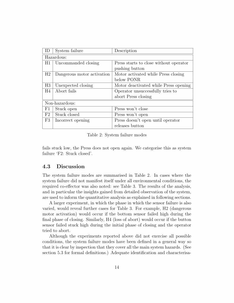
ID System failure Description

Hazardous:H1 Uncommanded closing Press starts to close without operator

pushing buttonH2 Dangerous motor activation Motor activated while Press closing

below PONRH3 Unexpected closing Motor deactivated while Press openingH4 Abort fails Operator unsuccessfully tries to

abort Press closing

Non-hazardous:F1 Stuck open Press won’t closeF2 Stuck closed Press won’t openF3 Incorrect opening Press doesn’t open until operator

releases button

Table 2: System failure modes

fails stuck low, the Press does not open again. We categorise this as systemfailure ‘F2: Stuck closed’.

4.3 Discussion

The system failure modes are summarised in Table 2. In cases where thesystem failure did not manifest itself under all environmental conditions, therequired co-effector was also noted: see Table 3. The results of the analysis,and in particular the insights gained from detailed observation of the system,are used to inform the quantitative analysis as explained in following sections.

A larger experiment, in which the phase in which the sensor failure is alsovaried, would reveal further cases for Table 3. For example, H2 (dangerousmotor activation) would occur if the bottom sensor failed high during thefinal phase of closing. Similarly, H4 (loss of abort) would occur if the buttonsensor failed stuck high during the initial phase of closing and the operatortried to abort.

Although the experiments reported above did not exercise all possibleconditions, the system failure modes have been defined in a general way sothat it is clear by inspection that they cover all the main system hazards. (Seesection 5.3 for formal definitions.) Adequate identification and characterisa-

14

Sensor Failure Co-effector Systemmode failure

Button stuck high H1stuck low F1

Bottom stuck high F1stuck low F2

Top stuck high Button pushed while opening H3Button released after Press closes F3

stuck low F1PONR stuck high Button released between top & PONR H4

stuck low Button released between PONR & bottom H2Button released after Press closes F3

Table 3: Partial Failure Modes and Effects Analysis

tion of hazards is an important pre-requisite for subsequent risk analysis, butis beyond the scope of the current paper.

As a final remark, it should be noted that the operational concept forthe Press from Section 3.1 can be implemented in several different ways, andthat the choice has a large effect on the risk analysis results. As explainedin Section 3.2, the “naive” control logic used in this paper is the following:

• if the plunger is at the bottom, or is above PONR and the button isreleased, turn the motor on

• if the plunger is at the top and the button is pushed, turn the motoroff

By contrast, Atchison et al [13, 16] use a control logic based on (an internalrepresentation of) the state of the Press along the following lines:

• if the Press is closed, or is closing above PONR and the button isreleased, turn the motor on

• if the Press is open and the button is pressed, turn the motor off

While the two logics are indistinguishable when sensors are functioning cor-rectly, they have very different behaviours in the presence of faults. Forexample, if the PONR sensor fails stuck low (indicating the plunger is abovethe PONR), then the Press will stay in the “closing above PONR” state in

15

the latter case, and the motor will not get turned on again until the operatorreleases the button. In our case however the motor gets turned on again assoon as the plunger reaches the bottom.

Grunkse et al [24] use the same control logic as us but a different modelof operator behaviour, in which the operator pushes and releases the buttonat a rate of once per 10 sec on average. This leads to quite different riskanalysis results for some failure modes, such as PONR stuck high. They alsoassume that sensor values are updated and processed without delay, whichis different from our treatment below (see Section 6.5.1 for details).

5 Stochastic model of the Press system

Having performed Hazard Identification and a form of Failure Modes andEffects Analysis, the next step is to develop stochastic models of the sys-tem, in order to quantify the different possible effects of component failuresand estimate the likelihood of hazardous system failure. This section beginswith a description of formulation of CTMCs in PRISM as background to ourmodels. It then outlines the PRISM model of the Press. Section 5.3 out-lines timing considerations and Section 5.7 describes how sensor failures aremodelled. The PRISM simulator was used to manually validate timing andprobability of individual transitions in the models reported below, to ensurethey approximated the behaviours of the plunger and operator described inSection 3.

5.1 Stochastic modelling in PRISM

CTMCs are specified as collections of interacting modules in PRISM, eachwith its own variable set, initial state and set of labelled transitions [14].Each transition is of the form

[e] guard -> r: var’=b

where e is an event label (used for synchronisation of transitions across dif-ferent modules; the event label is omitted if the transition is not required tosynchronise with transitions in other modules), guard is a Boolean expres-sions representing the guard of the transition, r is a rate (explained below),and b is the value of the variable var after the transition has taken place.The state of a module is determined by the current values of its variables.

16

The system state is the product of the individual module states. See [8] fora fuller description of the PRISM semantics.

In CTMCs, stochasticity is modelled using exponential functions for prob-ability and timing of transitions between pre- and post-states. The modellerspecifies a rate for each state transition. If in some state s a single transitionis enabled with rate r, then the probability that the system leaves that statebefore time t is given by the Cumulative Distribution Function (CDF)

Expx(t) = 1 − e−t/x (1)

where x = 1/r. (The case where multiple transitions are enabled simultane-ously is discussed below.) This treatment has some very nice mathematicalproperties. For example, the expected time that the system will stay in thepre-state s is x. (The actual transition to a post-state is taken to be instan-taneous.) If in particular the transition goes from a working state to a failedstate, then r is called a failure rate and x gives the Mean Time To Failure(MTTF).

For many aspects of our models below, ‘expected time in a state’ is amore natural concept than ‘rate’ so we tend to use x in preference to r whenexplaining the models below. Thus, we talk about sensors having a MTTFof 5 years, for example, when the transition leading to the failure state has aconstant failure rate of 1 in 5 years. We model different phases of the Pressoperational cycle as discrete states, with the expected time spent in eachstate defined according to the values given by the Modelica simulation ofplunger behaviour in Table 1 above. Thus for example, the transition fromstate ‘plunger falling above PONR’ to state ‘plunger falling below PONR’has a rate of 1/TTP, which results in an expected time of TTP = 1.78 secfor being in the state ‘plunger falling above PONR’.

Where transitions in two or more separate modules are synchronised (viathe event label), they take place simultaneously as a single system statetransition. The rate of the combined transition is the product of the rates ofthe individual transitions. Synchronised transitions can only be taken if theguards of all their individual transitions hold.

5.2 Race conditions

According to PRISM’s semantics of CTMCs, when two or more (non-synchronised)transitions are enabled simultaneously, one of the transitions is selected prob-

17

abilistically and then taken: i.e., there is a “race” between the different tran-sitions, with only one winner. Using the notation of [14], let S be the set ofall states in the full CTMC model and let R : S × S → R≥0 be its transitionrate matrix. The time spent in state s before any transition occurs is prob-abilistic with cumulative probability given by the CDF in formula 1 above,with rate r substituted by

E(s)def= Σs′∈S R(s, s′)

E(s) is called the exit rate for state s. The probability of making transitions 7→ s′ is given by

p(s, s′)def= R(s, s′)/E(s).

and the expected time spent in the pre-state s is 1/E(s).Note that this means that the timing behaviours of modules are not

independent: the time that a module spends in one of its states can beinfluenced by behaviours of other modules. This lack of “true modularity”means the modeller needs to be very careful when specifying rates. Weencountered this issue many times during modelling: cf. for example thediscussion of modelling of operator behaviour in Section 5.4, estimation ofImmediate Failure Likelihood in Section 6.2, and the possibility of hazardousbehaviour due to race conditions in Section 6.5.1.

In the following we outline our CTMC model of the Press. This model isdivided into modules corresponding to the main components of the system:the plunger, the operator, the four sensors, the control logic, and the motor-drive actuator.

5.3 Plunger behaviour

The plunger has six main physical states, according to its position and di-rection of travel (see Fig. 3): at bottom (state 1), rising below PONR (state3), rising above PONR (state 4), at top (state 5), falling above PONR (state7), and falling below PONR (state 8). Intermediate states 2, 6 and 9 are in-cluded in order to allow synchronisation of the actions of the different systemcomponents. (PRISM allows only one synchronisation event per transition.)So for example state 6 corresponds to the case where the motor has beenturned off while the plunger is at the top but the plunger has not yet fallenquite far enough for the top sensor to detect its changed state. States 10-13represent hazards H1-H4 respectively and are explained further below.

18

module Plunger

state : [1..13] init 1;

[motorOn] state=1 -> state’=2;

[plNotAtBottom] state=2 -> state’=3;

[plAbovePONR] state=3 -> RisingR1:(state’=4);

[motorOff] state=3 -> state’=12; // H3

[plAtTop] state=4 -> RisingR2:(state’=5);

[motorOff] state=4 -> state’=12; // H3

[motorOff] state=5 & stateOp=1 -> state’=10; // H1

[motorOff] state=5 & stateOp=2 -> state’=6;

[plNotAtTop] state=6 -> state’=7;

[plBelowPONR] state=7 & stateOp=1 -> FallingR4:(state’=13); // H4

[plBelowPONR] state=7 & stateOp=2 -> FallingR1:(state’=8);

[motorOn] state=7 -> state’=9; // abort above PONR

[plAtBottom] state=8 -> FallingR2:(state’=1);

[motorOn] state=8 -> state’=11; // H2

[] state=9 -> FallingR3:(state’=4);

endmodule

Figure 3: Plunger behaviour

19

ID System failure Description Plungerstate

H1 Uncommanded Motor deactivated while plunger 10closing at top and button released

H2 Dangerous motor Motor activated while plunger 11activation falling below PONR

H3 Unexpected Motor deactivated while plunger 12closing rising

H4 Abort fails Plunger falls past PONR without 13motor being activated, eventhough button was released

Table 4: Modelling of hazardous states

Most of the transitions in our plunger model are guarded by synchroni-sation events. These are depicted as labels on the transition edges in Fig. 3,using the convention of adding suffix ‘!’ or ‘?’ according to whether the eventis initiated by this component or by another component. (This notation isnot part of the PRISM language and is used here only to aid understanding.)For example, the plunger transitions from rising below PONR (state 3) torising above PONR (state 4) will synchronise with a change of state in thePONR sensor module using the event plAbovePONR.

Some transitions from states 5 and 7 are also guarded by a predicate whosevalue depends on the current state of the operator module: stateOp=1 in-dicates that the operator has released the button and stateOp=2 indicatesthat the operator is currently pushing the button (see Section 5.4 below).These guards are used to distinguish normal operation from hazardous be-haviour. For example, if the motor gets turned off while the Press is open(state 5) and the operator is pushing the button, this is normal behaviour.But if the operator is not pushing the button, this is hazardous behaviour(H1 Uncommanded closing).

The states 10-13 model the occurrence of hazards H1-H4: see Table 4.These states are terminal states with no outgoing edges, and thus they ab-stract from any further behaviour of the Press that might occur after thehazardous state occurs. Modelling the hazards in this way adds some com-plexity to the model but it makes formalisation in CSL very easy: we simplycheck the likelihood that the system reaches one of the hazardous states (see

20

Section 6 below).An abort by the operator is modelled as a transition from state 7 (falling

above PONR) to state 4 (rising above PONR) via an additional state 9in case the event mOn? is received. This is a slight simplification sincethe actual plunger behaviour will depend on how early during closing theoperator releases the button. If button release occurs late (but still beforePONR) then the motor will slow and eventually reverse the plunger’s fall, butthe plunger may pass the PONR in the interim. Rather than complicatingour model by introducing complex timing considerations and force/frictioncalculations, we simply ignore this phenomenon, since it does not impact ourmain risk calculations. This simplification is valid provided we don’t try toinfer anything about the plunger’s actual position during that phase of Pressoperation.

Similarly, we omitted the cases where a mOn? event is received in state6, or a mOff? event in state 2, in the interests of simplicity. They introducedloops into the model which significantly complicated the analysis, withoutsubstantively changing the results for the hazards we study.

Timing of the plunger’s behaviour

As explained above, in CTMCs all transitions are probabilistic and the sys-tem stays in a state for a non-zero period of time before transitioning to a newstate. The exponential CDF describes the timing, which is parametrised byrates (see equation 1). This section explains the choice of rates in the plungermodule.

The first step is to choose an appropriate unit of time for ‘simple’ (basic)transitions. In our model we chose to use the time taken to sense and transmitor process data, which is commonly called the clock rate. The actual choiceof clock rate is a parameter in our model, so that we can test the effectsof different design decisions. Faster clock rates reduce the likelihood of raceconditions, but can be harder or more expensive to achieve in practice, sobeing able to evaluate the risk associated with different rates is an importantcapability for trade-off analysis in system design. In Section 7.1.1 below weinvestigate a range of clock rates from 1,000 per sec to as high a rate as ourPRISM model would feasibly allow. For much of the analysis in the rest ofthe paper we settle on 10,000 per sec (clock=10−4). Where a rate is notexplicitly specified in a transition, it is taken to be the unit rate (i.e., theclock rate).

21

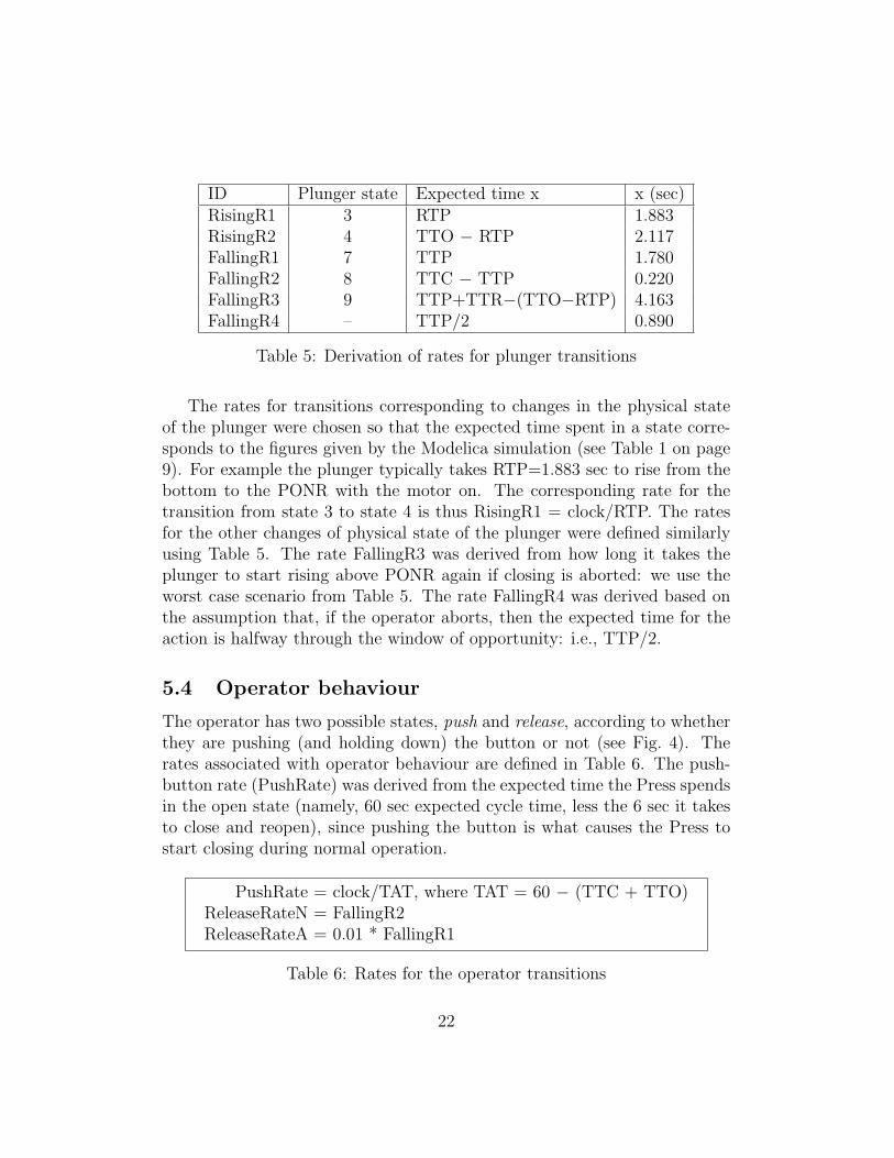
ID Plunger state Expected time x x (sec)RisingR1 3 RTP 1.883RisingR2 4 TTO − RTP 2.117FallingR1 7 TTP 1.780FallingR2 8 TTC − TTP 0.220FallingR3 9 TTP+TTR−(TTO−RTP) 4.163FallingR4 – TTP/2 0.890

Table 5: Derivation of rates for plunger transitions

The rates for transitions corresponding to changes in the physical stateof the plunger were chosen so that the expected time spent in a state corre-sponds to the figures given by the Modelica simulation (see Table 1 on page9). For example the plunger typically takes RTP=1.883 sec to rise from thebottom to the PONR with the motor on. The corresponding rate for thetransition from state 3 to state 4 is thus RisingR1 = clock/RTP. The ratesfor the other changes of physical state of the plunger were defined similarlyusing Table 5. The rate FallingR3 was derived from how long it takes theplunger to start rising above PONR again if closing is aborted: we use theworst case scenario from Table 5. The rate FallingR4 was derived based onthe assumption that, if the operator aborts, then the expected time for theaction is halfway through the window of opportunity: i.e., TTP/2.

5.4 Operator behaviour

The operator has two possible states, push and release, according to whetherthey are pushing (and holding down) the button or not (see Fig. 4). Therates associated with operator behaviour are defined in Table 6. The push-button rate (PushRate) was derived from the expected time the Press spendsin the open state (namely, 60 sec expected cycle time, less the 6 sec it takesto close and reopen), since pushing the button is what causes the Press tostart closing during normal operation.

PushRate = clock/TAT, where TAT = 60 − (TTC + TTO)ReleaseRateN = FallingR2ReleaseRateA = 0.01 * FallingR1

Table 6: Rates for the operator transitions

22

module Operator

stateOp : [1..2] init 1; // release(1), push(2)

[pushButton] stateOp=1

-> PushRate:(stateOp’=2);

[releaseButton] stateOp=2 & !(state=5 | state=6 | state=7)

-> ReleaseRateN:(stateOp’=1); // normal release

[releaseButton] stateOp=2 & (state=5 | state=6 | state=7)

-> ReleaseRateA:(stateOp’=1); // abort

endmodule

Figure 4: Operator behaviour

There are two different cases for when (and why) the operator releases thebutton. If they release the button while the Press is closing above PONR,this is an abort and we are told it typically occurs one in a hundred times.We model this by a transition which is only enabled when the plunger isin states 5-7 and whose rate (ReleaseRateA) is 0.01 times that associatedwith the plunger falling to the PONR (FallingR1). Thus, once the controlleractions are taken, there is a race between the plunger reaching PONR andthe operator releasing the button, which the PONR-reached-first case (i.e.,no abort operation) is 100 times more likely to win.

The other case is where the operator releases the button normally (i.e.,not while the Press is open or closing above PONR). In the absence of otherinformation, for the purposes of analysis we have assumed the operator isequally likely to release the button before or after the Press has fully closed.By setting the rate ReleaseRateN to be the same as the rate for the plunger

23

transition from falling-below-PONR to at-bottom, this makes the likelihoodthat they release the button before the plunger reaches the bottom fifty percent, as desired. (There is a small effect on the expected time spent in state8 in the case where the operator keeps pushing the button because of theway exit rates are defined in PRISM, but it is negligible for the purposes ofour analysis.)

5.5 Sensor and actuator normal behaviour

Sensors are modelled as simple components that detect a change in the stateof the environment (such as the plunger passing a given position, or the op-erator pushing or releasing the button) and output a signal to the controller.Actuators detect signals and cause changes to the environment, e.g., turningthe motor drive on or off.

module TopSensor

stateTS : [0..3] init 0; / high(1), low(3)

[plAtTop] stateTS=0 -> stateTS’=1;

[tsHigh] stateTS=1 -> stateTS’=2;

[plNotAtTop] stateTS=2 -> stateTS’=3;

[tsLow] stateTS=3 -> stateTS’=0;

endmodule

Figure 5: Top sensor behaviour

Fig. 5 shows the module of the top sensor. Initially the top sensor moduleis in state 0 and can receive event plAtTop? from the plunger, indicating ithas reached the top. When this event occurs the module transitions to state1 and sends the event tsHigh! to the controller. The sensor remains in thisstate until it receives event plNotAtTop? indicating the plunger has started

24

module Controller

stateC : [1..2] init 1; // motor off(1), motor on(2)

ts : [0..1] init 0;

bs : [0..1] init 1;

ps : [0..1] init 1;

button : [0..1] init 0; // released(0), pushed(1)

[buttonP] true -> button’=1;

[buttonR] true -> button’=0;

[psHigh] true -> ps’=1;

[psLow] true -> ps’=0;

[bsHigh] true -> bs’=1;

[bsLow] true -> bs’=0;

[tsHigh] true -> ts’=1;

[tsLow] true -> ts’=0;

[turnMOn] stateC=1 & (bs=1 | (button=0 & ps=0)) -> stateC’=2;

[turnMOff] stateC=2 & ts=1 & button=1 -> stateC’=1;

endmodule

Figure 6: PRISM code of the controller behaviour

to fall. In response the top sensor sends the event tsLow! to the controllerand transitions to state 0 again. All these transitions have unit rate. Themodules for the other sensors and the motor drive actuator are analogous tothe above. They synchronise alternately with the plunger and the controller,reacting to one and causing a change in the other as a result (at least, whenthey are functioning correctly). The PRISM code for the other sensors andthe motor component are listed in Appendix B.

5.6 Controller behaviour

The controller component keeps track of the signals it has received from thesensors and the state of the motor drive, and sends a signal to the motordrive as described in Section 3.2 above (see Fig. 6). The controller storesthe current state of the sensors internally using local variables ts, bs, ps,button. Their values are updated each time a signal is received from thesensor components via the corresponding synchronisation event.

25

module TopSensor

stateTS : [0..6] init 0;

[plAtTop] stateTS=0 -> stateTS’=1;

[tsHigh] stateTS=1 -> stateTS’=2;

[plNotAtTop] stateTS=2 -> stateTS’=3;

[tsLow] stateTS=3 -> stateTS’=0; // as before up to here

[tsFailsHigh] !(stateTS=4 | stateTS=5 | stateTS=6)

-> sensorFail: stateTS’=4;

[tsHigh] stateTS=4 -> stateTS’=6;

[tsFailsLow] !(stateTS=4 | stateTS=5 | stateTS=6)

-> sensorFail: stateTS’=5;

[tsLow] stateTS=5 -> stateTS’=6;

[plAtTop] stateTS=6 -> stateTS’=6;

[plNotAtTop] stateTS=6 -> stateTS’=6;

endmodule

Figure 7: Top sensor behaviour with both failure modes included

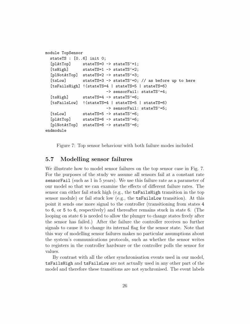
5.7 Modelling sensor failures

We illustrate how to model sensor failures on the top sensor case in Fig. 7.For the purposes of the study we assume all sensors fail at a constant ratesensorFail (such as 1 in 5 years). We use this failure rate as a parameter ofour model so that we can examine the effects of different failure rates. Thesensor can either fail stuck high (e.g., the tsFailsHigh transition in the topsensor module) or fail stuck low (e.g., the tsFailsLow transition). At thispoint it sends one more signal to the controller (transitioning from states 4

to 6, or 5 to 6, respectively) and thereafter remains stuck in state 6. (Thelooping on state 6 is needed to allow the plunger to change states freely afterthe sensor has failed.) After the failure the controller receives no furthersignals to cause it to change its internal flag for the sensor state. Note thatthis way of modelling sensor failures makes no particular assumptions aboutthe system’s communications protocols, such as whether the sensor writesto registers in the controller hardware or the controller polls the sensor forvalues.

By contrast with all the other synchronisation events used in our model,tsFailsHigh and tsFailsLow are not actually used in any other part of themodel and therefore these transitions are not synchronised. The event labels

26

were introduced to help in debugging and validating the model using thePRISM simulator and model checker.

When we do FMEA below only one sensor failure mode will be enabledat a time. Thus for example, when we investigate the risk associated withbottom sensor failing stuck high, we use the modules for the normal (fault-free) behaviour of the other sensors (such as Fig. 5 for the top sensor) anda copy of the module for faulty behaviour for the bottom sensor with thebsFailsLow failure transition removed. Similarly, when we do analysis ofmultiple failure modes, we include only the relevant failure transitions.

6 Risk Analysis

This section describes the basis on which the risk calculations are performed,including how various system properties can be formalised for model checkingin Continuous Stochastic Logic (CSL) [10], the formal language in whichproperties of CTMCs are formulated for model checking in PRISM.

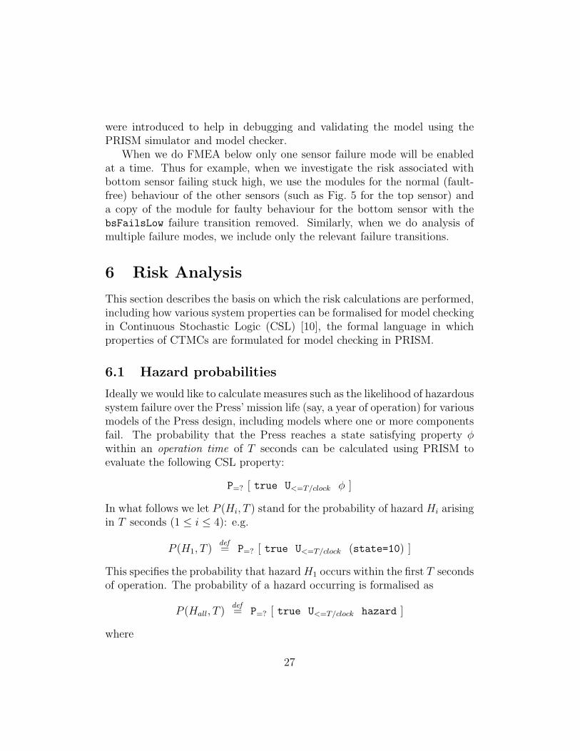
6.1 Hazard probabilities

Ideally we would like to calculate measures such as the likelihood of hazardoussystem failure over the Press’ mission life (say, a year of operation) for variousmodels of the Press design, including models where one or more componentsfail. The probability that the Press reaches a state satisfying property φwithin an operation time of T seconds can be calculated using PRISM toevaluate the following CSL property:

P=? [ true U<=T/clock φ ]

In what follows we let P (Hi, T ) stand for the probability of hazard Hi arisingin T seconds (1 ≤ i ≤ 4): e.g.

P (H1, T )def= P=? [ true U<=T/clock (state=10) ]

This specifies the probability that hazard H1 occurs within the first T secondsof operation. The probability of a hazard occurring is formalised as

P (Hall, T )def= P=? [ true U<=T/clock hazard ]

where

27

hazarddef= (state=10 | state=11 | state=12 | state=13)

In assessing risk hazards are usually weighted according to their severity buthere we simply treat them all equally; thus P (Hall, T ) represents the risk ofhazardous system failure in operation up to time T .

Ideally we want to calculate P (Hi, 1yr) under different assumptions aboutsensor failure rates, say with a mean time to failure of 5 years each. As shownin Section 7.1.2 below, however, such calculations are not computationallyfeasible for our models. So instead we decompose the problem into two partsas follows:

• the Immediate Failure Likelihood (IFL) and

• the Mean Time to Failure (MTTF)

where “failure” refers to hazardous system failure in both cases.Immediate Failure Likelihood is an estimate of how likely the component

failure is to lead to a hazardous system failure in the short term, namelywithin 60 sec in what follows. We need to consider a non-zero time framebecause of the continuous-time nature of CTCMs. We chose 60 sec because itis the length of typical operational cycle of the Press, but other times couldhave been used. The notion is defined more precisely in the next section,together with a method for calculating it.

Mean Time to Failure, on the other hand, is an estimate of the expectednumber of operational cycles the system completes before hazardous failure.For component failures that usually reveal themselves immediately or aftera short delay, the result will be less than 1. But for failures which maystay hidden for some time after the component fails, and are only revealedwhen particular combinations of circumstances arise, the result can be greaterthan 1. Hidden failures can be particularly nasty because, although theirlikelihood may be low in a single operational cycle, they are in some sense“just waiting to happen”. The fault propagation mechanisms involved areoften subtle and difficult for the designer to anticipate because they involveunusual combinations of circumstances, so having a way of identifying theirpresence is very valuable. Section 6.3 below describes a method for usingPRISM to calculate MTTF and discusses some of the issues involved.

28

6.2 Revealed failures and Immediate Failure Likeli-hood

We define the Immediate Failure Likelihood for a given sensor failure modeand hazard Hi to be

IFLdef= PM(Hi, 60) (2)

where M is the CTMC model with the particular sensor failure mode enabledand with a sensor failure rate of 1/60 sec. We show below that IFL is areasonable estimate of the likelihood that hazardous system failure Hi occurswithin 60 secs (one typical operational cycle) of the sensor failing.

We need to explain why we use a sensor failure rate of 1/60 sec in PM .As shown in Section 4, a sensor failure can have different consequences de-pending on the phase of operation in which it occurs. In the absence of otherinformation, it is reasonable to assume that a sensor failure is equally likelyto occur any time during the operation cycle, and thereby to use a linearcumulative distribution function (CDF) for the probability of occurrence.However, because we are using a CTMC modelling framework, we must in-stead use the exponential CDF from formula (1) on page 17 and select avalue for the sensor failure rate sensorFail to approximate the linear CDF.We show below that one per 60 sec gives a reasonable estimate.

First note that, if the failure is equally likely to take place at any time,then the probability that it occurs during a phase of operation that typicallytakes T sec would be T/60. We consider each phase of operation in turn andshow that the above model gives a reasonable approximation to this figure.We use the notation from Section 5.2.

First consider the case where, apart from the sensor failure transition,only a single simple unit transition is enabled (e.g., [motorOn] state=1 ->

state’=2). In this case the transition rate relation R(s, .) is dominated by theunit rate (1 � sensorFail = clock/60), so E(s) ≈ 1. The likelihood that thefailure occurs in this case is p(s, s′) ≈ sensorFail, where s′ is the state wherethe sensor has failed. More generally, when R(s, .) is dominated by a singlevalue η � sensorFail, then E(s) ≈ η and the probability that the failureoccurs is approximately sensorFail/η. (Note also that the expected timespent in the pre-state is approximately clock/η, no matter which transitionis taken.)

Now consider the case where the plunger is rising below PONR andall enabled unit transitions have been taken. Inspection by hand, or us-

29

ing the PRISM simulator, shows that R(s, .) is dominated by the tran-sition [plAbovePONR] state=3 -> RisingR1:(state’=4) that takes theplunger past PONR, with rate RisingR1. Since RisingR1 = clock/RTP �sensorFail, then E(s) ≈ RisingR1 and the probability that the sensor failsin this case is approximately sensorFail/RisingR1 = RTP/60, as desired.

Similar calculations show that, for a plunger transition which is expectedto take T seconds with T � 60, the probability that the sensor fails in thatphase is approximately T/60, as desired.

The final case to consider is where the Press is open, waiting for theoperator to push the button. In this case the push-button rate PushRate =clock/54 is close in value to sensorFail. That means there are two possibletransitions from this state (the button can get pushed or the sensor can fail),each with approximately the same probability. Thus E(s) ≈ 2× sensorFailand the probability that the sensor fails is approximately 1/2. The linearCDF on the other hand gives 54/60 for the probability that the sensor failsduring this phase of operation and we can see that the approximation is notvery good. The trade-off in improving the approximation is to complicatethe model. For the purposes of this paper, we have taken the approach ofkeeping the model relatively simple and readable, at the expense of someprecision in this case.

Note also that the expected time spent in the Press-open state beforethe next transition occurs is clock/E ≈ clock/(2 × sensorFail) = 30 sec.Our failure models thus effectively simulate a shorter operational cycle timethan desired. There seems to be no easy way to resolve this problem withoutsubstantially complicating the model. However, since we are only interestedin estimating the relative effects of design changes, and are careful not tomake assertions about absolute probabilities, we prefer to stick with a rel-atively simple model of components and interactions. This discussion doeshowever illustrate some of the sometimes unanticipated timing interactionsand subtleties of using CTMCs to model stochastic systems.

The final point to note is that the probability that the sensor actuallyfails in the first 60 sec is Exp60(60) = 0.63. Our method of calculating IFLthus underestimates even this simple possibility. But again there seems tobe no easy way to resolve this issue. In Section 7.2.2 below we performa sensitivity analysis to show that, although the approximation can affectresults (e.g., under-reading by as much as 37% in some cases), the RoughOrder of Magnitude (ROM) is not affected. It is thus valid to use the resultsto investigate the relative effect of different design choices on the ROM of

30

hazardous failures.In summary, using a sensor failure rate of 1 per 60 sec seems to give

the fairest comparison of the immediate risk, since it makes the likelihoodof occurrence of sensor failure closely proportional to the time spent in thevarious phases of operation, other than the Press-open phase. But it isimportant to note that IFL is only an approximation, and should not beregarded as an actual probability of failure.

6.3 Hidden failures and MTTF calculations

The second case of quantitative risk analysis formalised here relates to hiddenfailures. These are failures where the fault lies dormant and is only revealedwhen suitable co-effectors are present. (Race conditions can also play a part,when they result in sensor data being received late. These are discussedfurther in Section 6.5.1 below.)

To some extent, the likelihood of such failures is already taken into ac-count in the IFL calculation described above. For example, if the PONRsensor fails high, then the system appears to behave normally, as long as theoperator does not attempt to abort operation (represented by the coeffectorwhereby the button is released while the plunger is falling above the PONR).The likelihood of the latter (1 in 100) is taken into account in the operatormodel in Section 5.4. Thus the likelihood of this case occurring within 60sec of the sensor failing is taken into account in the calculation of IFL above.However, the fault will not be revealed until the operator tries to abort oper-ation, and only then will the system failure (H4 loss of abort) occur – quitepossibly under precisely the circumstances when abort is actually needed forsafety reasons.

To investigate such failures we used PRISM’s rewards mechanism [14]to calculate the Mean Time to Failure (MTTF) for hazardous failures. Weextend the model with a reward matrix which applies a transition reward of 1unit each time the Press closes (i.e., when the transition from state 8 to state 1in the plunger model occurs), representing completion of an operational cycle.Then the MTTF R is calculated by evaluating the following reachabilityreward property [8]:

Rdef= R=? [ F hazard ] (3)

In cases where the probability of not reaching a hazardous state approacheszero as time increases (e.g., if on any path a hazard can eventually be

31

reached), then R evaluates to a finite number representing the expected num-ber of operational cycles completed before a hazard occurs.

Unlike P (H, T ) above, PRISM is able to estimate R in a reasonably shorttime for very low sensor failure rates, and independent of the mission time.This makes it attractive for use during model development and debugging. Asit turns out however, when low sensor failure rates (such as one per 5 years)are used, we find that system failures are dominated by race conditions, andthere is not much difference in calculated MTTF between the results forfault-free behaviour and behaviour when sensor faults may be present. (Thismay also be due in part to inaccuracies in the numerical analysis methodsused. Such inaccuracies tend to accumulate in CTMC models when thereare large differences in the rates involved in different transitions [11], such asin our case.)

Instead or relying on such results, we propose the following heuristic fordetermining whether a failure is revealed in the short term or more likelyto stay hidden. Just as for IFL above, we set the sensor failure rate to oneper 60 sec and evaluate R for each failure mode in turn. For failures whichare likely to be revealed within one operational cycle, R will evaluate to lessthan 1.0. If R is finite but greater than 1, on the other hand, this indicatesthat the system is likely to keep operating, and fail hazardously at some latertime, when the required coeffectors occur.

In this last case, the value of R can often be used to help determinewhich coeffector must be involved. If a single coeffector is involved, and itoccurs with probability p per cycle (p � 1), then R will be approximately1/p. Thus for example, for the PONR sensor stuck high failure noted above,R is approximately 100 (see Section 7.2.3), which is the expected numberof operational cycles before abort occurs. R thus gives a strong clue as towhat coeffectors to investigate. When R is very high, however, it typicallyindicates that race conditions are the issue, and it is necessary instead touse the PRISM animator (or some other method) to discover what faultpropagation mechanisms are involved.

The success of the approach depends however on the system not havingnon-hazardous long-term behaviours with non-zero probability, because insuch cases R evaluates to infinity. For example, if there is a non-zero prob-ability that the Press will get into a stuck open or stuck closed situation(such as after a button stuck low failure), then R = ∞ and this methodcannot be used to estimate MTTF. Therefore, the approach does not han-dle the non-hazardous system failures F1 (stuck open), F2 (stuck closed)

32

and F3 (incorrect opening) from Table 2. But conversely, an infinite valueof R for our models indicates that a cycle exists (i.e., the press gets stuckopen or stuck closed), and the PRISM animator can be used to discover thefailure mechanism that gives rise to it. It is not clear to what extent thisphenomenon can be generalised to other models however, since it is seems tobe more due to good luck than good modelling for the Press study.

In summary then, using formula (3) to calculate the mean time to haz-ardous failure for a sensor failure mode with failure rate 1/60 sec gives auseful heuristic for discovering hidden failures. But as usual with these kindsof calculations, the results need careful interpretation. They should not beinterpreted as an accurate estimation of mean time to hazardous systemfailure.

6.4 Likelihood of hazardous system failure

Returning to the original problem, the challenge was to estimate the risk ofhazardous failure over a mission time of 1 yr with sensor failure rates of 1per 5 yr, say. For sensor failure modes that are most likely to be revealedin the short term (MTTF ≤ 1), the hazard risk likelihood is roughly thelikelihood of sensor failure multiplied by IFL. (When IFL is small, the morelikely outcome is a non-hazardous system failure in this case.) The likelihoodof sensor failure is Exp5yr(1yr) ≈ 0.18 from formula (1) on page 17.

For hidden failures on the other hand (MTTF between 1 and say 1000),the hazard risk likelihood is simply the likelihood of sensor failure itself, sincethe fault condition remains in place until the coeffector occurs, and the lattercan usually be assumed to occur at least once during the rest of the system’smission time.

In situations where system failures are dominated by race conditions, thesituation lies somewhere between these two extremes. See Section 6.5.1 formore discussion.

6.5 Other remarks

Before turning to the results of our PRISM analysis, some further remarksabout strengths and weaknesses of the approach are in order.

33

6.5.1 Race conditions in fault-free operation

The first remark concerns the presence of race conditions in our models, in-cluding our baseline “fault-free” model of Press operation. In many systemstates, a “fast” transition (such as involved in data transmission and/or pro-cessing) can be enabled at the same time as a “slow” transition (such as theplunger rising from the bottom to the PONR), with a non-zero probabilitythat the slow transition will be taken first, or instead of, the fast transition.As a result, hazards can occur with non-zero probability even when all thecomponents are functioning correctly.

For example, consider the system state immediately after a normal abort:i.e., [releaseButton] occurs while state=7 & stateC=2 & stateOp=1. Inthe first, much more common case, the sequence of subsequent events wouldbe [buttonR, turnMOn, motorOn], resulting in state=9 and successfulabort. But an alternative sequence of events with non-zero probability is[plBelowPONR, buttonR, turnMOn, motorOn], which results in state=11

(hazard H2: dangerous motor activation). This corresponds to the case wherethe plunger passes PONR before the control system gets a chance to turn onthe motor.

Although to some degree such behaviours are an artifact of the modellingapproach used, they do in fact occur in real life, and should be taken intoaccount in risk analysis and design for safety [39]. For this reason fault-freeoperation (i.e., without sensor failures) is also included in the analysis below.We note in passing that the methods discussed in this paper can be appliedwithout considering sensor-update race conditions if desired, by tweaking themodels to give “internal” controller actions priority over other actions. Thisis the approach taken in Grunske et al [24] for example.

6.5.2 Modelling non-hazardous system failures

As noted above, PRISM uses CSL as the formal language in which proper-ties of CTMCs are formulated for model checking. The cause-consequencerelation between component failure events and system hazards was easy toformulate in CSL because of the way we modelled component failure eventsas transitions (e.g. tsFailsHigh) and hazards as absorbing states (although,as remarked in Section 6.2, modelling of the timing of component failurespresented issues).

One drawback of using CMTCs we encountered, however, was that we

34

could find no simple way to capture the non-hazardous system failures F1(stuck open), F2 (stuck closed) and F3 (incorrect opening) in the model orin CSL. Part of the difficulty was due to the CTMC way of modelling timingindirectly using the exponential CDF and rates, and the need to specify atime frame over which probability is calculated. The fact that an event hasnot taken place within x sec does not imply that it will not take place withinx + δ sec. We have not found a way of formulating F1–F3 in CSL, nor werewe able to identify a suitable way of representing F1–F3 as absorbing statesin the plunger model. We investigated PRISM’s steady-state operator [8] asa possible solution, but calculating the probability of steady-state behaviourproved computationally infeasible for our model: the model checking processdid not terminate.

As a result we have had to omit some of the sensor failure modes from ourMTTF analysis below, as well as omitting F1–F3 from quantitative analysismore generally.

6.5.3 Other failure scenarios

As noted above, FMEA is typically conducted only for single componentfailures because of the difficulty of analysing system behaviour in the presenceof multiple failures and the combinatorial complexity of considering all thedifferent cases that arise [4]. One of the advantages of our approach is thatto model multiple failures it is simply a matter of including versions of thesensor modules with the appropriate failure events enabled.

It is also straightforward to model a wide range of other failure scenariossuch as common cause failures. For example, suppose it is found that thebottom sensor does not fail randomly but is in fact far more likely to failwhen the plunger hits it. More specifically, suppose that the bottom sensorfails stuck high when the plunger reaches the bottom with probability 1 in10,000. This could be modelled by adding the following transition to thebottom sensor module:

[bsFailsHigh] state=1 & !(stateBS=4 | stateBS=5 | stateBS=6)

-> bsFail: stateBS’=4;

with bsFail = 0.0001. In the rest of the paper however we focus primarilyon risk associated with single sensor failures.

35

6.5.4 PRISM settings

In the results reported below we used the Gauss-Seidel iteration settingwith termination epsilon set to 1E-6. This is an iterative numerical solu-tion method, so 100% accuracy cannot be assumed, especially in computa-tions which converge slowly (such as for high non-infinite values of rewardR and low non-zero values of IFL) because of cumulative rounding errors[11]. PRISM provides steady-state detection by default, which in many casesconsiderably shortens computation time through use of approximation topredict convergence. In our modelling and analysis, however, we needed todeactivate this facility since it gave misleading results in some cases.

All our experiments were performed on a standard PC with an IntelPentium 4 CPU 3GHz processor with Ubuntu 7.10 Linux as operating system.Probability results are rounded to two significant figures in the results below.

7 Results for the initial design of the Press

This section reports the results of our calculation of Immediate Failure Like-lihood (IFL) and Mean Time To Failure (MTTF) for the Press system asmodelled in Section 5, for normal “fault-free” operation and for the effectsof individual sensor failure modes. It also reports on computation time andvarious sensitivity analyses along the way to establishing a baseline referencemodel against which the effects of different design decisions will be evaluatedin later sections.

7.1 Fault-free operation

We first consider the case where sensors function correctly. Hazards cansometimes arise under these circumstances due to race conditions, as dis-cussed in Section 6.5.1. Using the PRISM animator we found the followingexamples of how race conditions could give rise to each of the hazards fromTable 4:

H1 (uncommanded closing) could occur if the operator pushes the buttonwhile the Press is open and then releases it again while the controlsystem is turning the motor off but before the plunger has droppedbelow the top sensor.

36

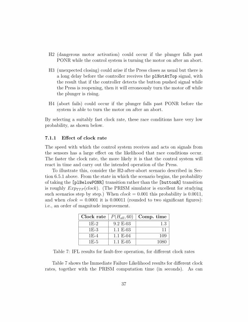
H2 (dangerous motor activation) could occur if the plunger falls pastPONR while the control system is turning the motor on after an abort.

H3 (unexpected closing) could arise if the Press closes as usual but there isa long delay before the controller receives the plNotAtTop signal, withthe result that if the controller detects the button pushed signal whilethe Press is reopening, then it will erroneously turn the motor off whilethe plunger is rising.

H4 (abort fails) could occur if the plunger falls past PONR before thesystem is able to turn the motor on after an abort.

By selecting a suitably fast clock rate, these race conditions have very lowprobability, as shown below.

7.1.1 Effect of clock rate

The speed with which the control system receives and acts on signals fromthe sensors has a large effect on the likelihood that race conditions occur.The faster the clock rate, the more likely it is that the control system willreact in time and carry out the intended operation of the Press.

To illustrate this, consider the H2-after-abort scenario described in Sec-tion 6.5.1 above. From the state in which the scenario begins, the probabilityof taking the [plBelowPONR] transition rather than the [buttonR] transitionis roughly ExpTTP (clock). (The PRISM simulator is excellent for studyingsuch scenarios step by step.) When clock = 0.001 this probability is 0.0011,and when clock = 0.0001 it is 0.00011 (rounded to two significant figures):i.e., an order of magnitude improvement.

Clock rate P (Hall, 60) Comp. time

1E-2 9.2 E-03 1.31E-3 1.1 E-03 111E-4 1.1 E-04 1091E-5 1.1 E-05 1080

Table 7: IFL results for fault-free operation, for different clock rates

Table 7 shows the Immediate Failure Likelihood results for different clockrates, together with the PRISM computation time (in seconds). As can

37

be seen, the probability of any of the hazards occurring decreases roughlylinearly with clock rate, whereas the computation time increases roughlylinearly.

Clock rate R (# operations) Comp. time

1E-3 845 141E-4 7,582 701E-5 39,845 1831E-6 69,444 244

Table 8: MTTF results for fault-free operation, for different clock rates

Table 8 shows the effect of different clock rates on MTTF, measured asexpected number R of completed operational cycles before hazardous failure.Note that R increases as the clock rate gets faster, since the likelihood of un-usual race conditions decreases, as anticipated. In fact, R is roughly inverselyproportional to P (Hall, 60). Another point to note is that the computationtime for R is much less affected by the clock rate than was the computationtime for P (Hall, 60), which suggests that the MTTF approach scales betterthan the IFL approach.

Because the purpose of this paper is to explore the potential benefitsand limitations of stochastic model checking, in what follows we have chosento focus primarily on a clock rate of 1E-4 per sec: i.e., a unit transitionhas an expected duration of 0.0001 sec. The resulting computation timemakes for reasonable turnaround time in experiments. In reality however,a higher-performance system architecture would probably be chosen for thePress, using a suitably fast processor, sensors and actuators. Unless explicitlystated otherwise, 1E-4 per sec is used as the default clock rate below.

7.1.2 Effect of operation time

Table 9 shows the effect of varying the operation time T (given in seconds),broken down by the different hazards. We consider an operation time T cor-responding to 1-4 typical operational cycles, respectively. The likelihood of ahazard occurring within T seconds rises roughly linearly with the operationtime, as we would expect. The longer we observe the system, the more likelythe occurrence of a hazard becomes. Likewise, the computation time (givenin seconds) rises roughly linearly with the operation time. One implication

38

T P (Hall, T ) P (H1, T ) P (H2, T ) P (H3, T ) P (H4, T )Comp.time

60 1.1 E-04 2.2 E-06 1.0 E-04 1.5 E-09 3.1 E-06 115 - 149120 2.3 E-04 4.0 E-06 2.2 E-04 3.2 E-09 6.4 E-06 220 - 283180 3.5 E-04 5.9 E-06 3.3 E-04 4.8 E-09 9.8 E-06 327 - 428240 4.6 E-04 7.8 E-06 4.4 E-04 6.4 E-09 1.3 E-05 434 - 564

Table 9: Probability of hazard arising in first T seconds of fault-free operation

of the latter observation is that the extent to which it is feasible to use thisapproach for calculating risk of failure over a longer time period is very lim-ited. It would not be feasible to use it to calculate risk over the system’smission lifetime (say T = 1yr), for example.

Although there is theoretically no limit specified for the value of T , inpractice the maximum value to be chosen depends on the model in questionand how long the user is willing to wait for results. For high values of Tthe accuracy of results can also be degraded due to approximations used infloating point arithmetic.

7.2 Failure Modes and Effects Analysis

This section summarises and discusses the results of model checking for eachof the sensor failure modes. In what follows we assume we are working witha model M in which a single sensor failure is enabled.

7.2.1 Immediate Failure Likelihood

Table 10 shows the IFL results for the different sensor failure modes. Theresults for fault-free operation are also included for comparison. The com-putation time for the failure-mode experiments is of the order of 300-700seconds. The boldface entries indicate the sensor failure modes that lead tosubstantially increased hazard risk over fault-free operation.

The results provide valuable insights into the relative likelihood of thedifferent scenarios. The boldface cases correspond closely to the hazardouscause-consequence relationships revealed in Table 3 on page 15 (with theadditional remarks in Section 4.3). Some of these cases are discussed in moredetail below. The cases where the hazard probabilities in the presence of

39

Failure mode P(Hall,60) P(H1,60) P(H2,60) P(H3,60) P(H4,60)

None 1.1 E-4 2.2 E-6 1.0 E-4 1.5 E-9 3.1 E-6

Button high 6.3 E-1 6.3 E-1 6.2 E-5 9.4 E-10 1.6E-4stuck low 6.8 E-5 1.5 E-6 6.4 E-5 9.4 E-10 1.9 E-6Bottom high 6.5 E-2 4.9 E-6 2.1 E-3 6.2 E-2 1.9 E-6stuck low 9.8 E-5 1.7 E-6 9.4 E-5 9.4 E-10 2.8 E-6Top high 1.7 E-1 1.7 E-6 9.7 E-5 1.7 E-1 2.9 E-6stuck low 6.8 E-5 1.5 E-6 6.4 E-5 9.4 E-10 1.9 E-6PONR high 3.5 E-3 2.2 E-6 6.2 E-5 1.5 E-9 3.5 E-3stuck low 1.6 E-1 2.0 E-6 1.6 E-1 1.5 E-9 2.9 E-6

Table 10: IFL results for Press with initial design

sensor failures are less than for fault-free operation correspond to the caseswhere non-hazardous system failures are the more likely outcome.

Some of the inaccuracies due to the approximations used in calculatingIFL noted in Section 6.2 become evident here. For example, if the buttonsensor is equally likely to fail high at any time during an operational cycleof the Press, then its likelihood of failing while the Press is open is about54/60; this case will lead immediately to hazard H1 (uncommanded closing).In fact, H1 is the most likely outcome in all cases of this failure mode, otherthan when it fails while falling above PONR and the user aborts, in whichcase H4 will occur instead. The actual probability of H1 should thus be closeto 1 for this case, whereas the IFL calculation gives a likelihood of 0.63. Thedifference is due to the possibility that the sensor may not fail at all withintthe first 60 sec.

Perhaps the most surprising result is that H3 (unexpected closing) isquite likely to occur if the bottom sensor fails high. The Modelica modelsimply predicted that the Press would get stuck open in this case. Furtherreflection (and using PRISM’s animator) reveals the following race-conditionscenario under which H3 can occur: The Press starts closing as usual (eventplNotATTop) but before the controller receives and acts on the top-sensor lowsignal (event tsLow), it instead thinks the Press is closed (because bs=1) andso turns the motor on, resulting in the plunger passing through states 7 and9 to 4 as though closing was being aborted; but then finally the controllerreacts to tsLow and turns the motor off, resulting in H3. This is a goodexample of how model checking can reveal hazardous behaviours that could

40

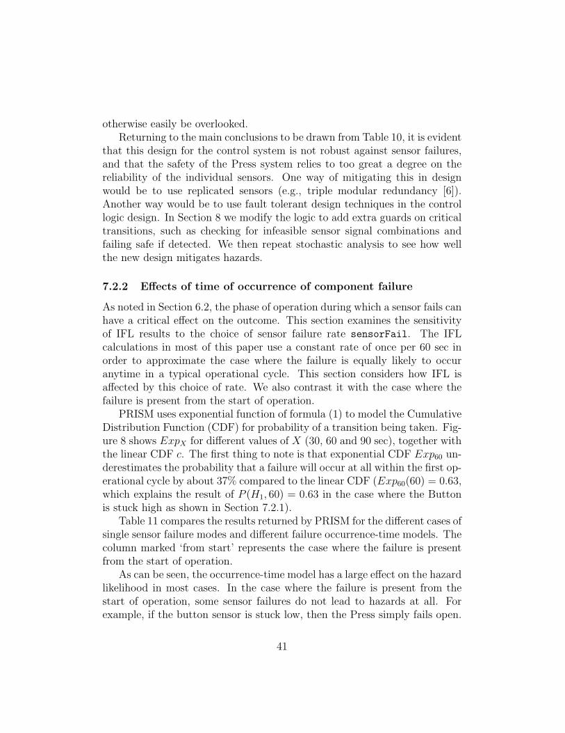
otherwise easily be overlooked.Returning to the main conclusions to be drawn from Table 10, it is evident

that this design for the control system is not robust against sensor failures,and that the safety of the Press system relies to too great a degree on thereliability of the individual sensors. One way of mitigating this in designwould be to use replicated sensors (e.g., triple modular redundancy [6]).Another way would be to use fault tolerant design techniques in the controllogic design. In Section 8 we modify the logic to add extra guards on criticaltransitions, such as checking for infeasible sensor signal combinations andfailing safe if detected. We then repeat stochastic analysis to see how wellthe new design mitigates hazards.

7.2.2 Effects of time of occurrence of component failure

As noted in Section 6.2, the phase of operation during which a sensor fails canhave a critical effect on the outcome. This section examines the sensitivityof IFL results to the choice of sensor failure rate sensorFail. The IFLcalculations in most of this paper use a constant rate of once per 60 sec inorder to approximate the case where the failure is equally likely to occuranytime in a typical operational cycle. This section considers how IFL isaffected by this choice of rate. We also contrast it with the case where thefailure is present from the start of operation.

PRISM uses exponential function of formula (1) to model the CumulativeDistribution Function (CDF) for probability of a transition being taken. Fig-ure 8 shows ExpX for different values of X (30, 60 and 90 sec), together withthe linear CDF c. The first thing to note is that exponential CDF Exp60 un-derestimates the probability that a failure will occur at all within the first op-erational cycle by about 37% compared to the linear CDF (Exp60(60) = 0.63,which explains the result of P (H1, 60) = 0.63 in the case where the Buttonis stuck high as shown in Section 7.2.1).

Table 11 compares the results returned by PRISM for the different cases ofsingle sensor failure modes and different failure occurrence-time models. Thecolumn marked ‘from start’ represents the case where the failure is presentfrom the start of operation.

As can be seen, the occurrence-time model has a large effect on the hazardlikelihood in most cases. In the case where the failure is present from thestart of operation, some sensor failures do not lead to hazards at all. Forexample, if the button sensor is stuck low, then the Press simply fails open.

41

Figure 8: Some models of CDF for time of failure occurrence in operationalcycle

Using the ‘from start’ model of sensor failure thus completely overlooks thecase where the button sensor fails low during closing, which could in turnlead to hazard H4 (abort fails). In the case of the button being stuck high,Exp30, representing behaviour where the failure is more likely to occur earlyin the operational cycle (expected time = 30 sec), gives a higher estimate ofrisk than Exp60, where the failure is likely to occur later in the operationalcycle. If the button is likely to fail early in the cycle then hazard H1 is morelikely to occur. On the other hand, Exp30 leads to a lower estimate in thebutton stuck low case than Exp60 because an early occurrence of this failureleads to the Press failing open rather than a hazard.

But the important thing to note is that the rough order of magnitude(ROM) is the same in each case other than the ‘from start’ case. As arguedin Section 6.2 above, using a sensor failure rate of one per 60 sec to calculateIFL is the most reasonable compromise.

7.2.3 Mean Time To Failure

Table 12 shows the Mean Time To Failure for hazardous failures, as explainedin Section 6.3. The result was ∞ for the cases that are missing from the table(button, bottom and top sensor stuck low): in such cases there are non-

42

Model: Exp1 Exp30 Exp60 Exp90 fromFailure mode start

Button stuck high 1.0 E+0 8.6 E-1 6.3 E-1 4.8 E-1 1.0 E+0Button stuck low 3.3 E-7 4.5 E-5 6.8 E-5 7.9 E-5 0.0 E+0Bottom stuck high 1.6 E-1 9.9 E-2 6.5 E-2 4.8 E-2 1.6 E-1Bottom stuck low 7.5 E-5 9.2 E-5 9.8 E-5 1.0 E-4 3.7 E-5Top stuck high 4.3 E-1 2.6 E-1 1.7 E-1 1.3 E-1 4.4 E-1Top stuck low 3.3 E-7 4.5 E-5 6.8 E-5 7.9 E-5 0.0 E+0PONR stuck high 8.8 E-3 5.4 E-3 3.5 E-3 2.6 E-3 8.8 E-3PONR stuck low 3.8 E-1 2.4 E-1 1.6 E-1 1.2 E-1 3.8 E-1

Table 11: Sensitivity of PM(Hall, 60) to models for time of failure occurrencein cycle

Sensor MTTF 1 min 10 min 100 min 5 yr

Fault-free operation 7,581

Button stuck high 0.9 10 98 7,560Bottom stuck high 0.9 10 98 7,560Top stuck high 2.8 12 100 7,560PONR stuck high 102 111 199 7,560PONR stuck low 1.9 11 99 7,560

Comp. time (secs) 2-7 3-7 8-12 145-211

Table 12: MTTF for initial design measured in number of cycles, with dif-ferent sensor reliability values

hazardous long-term behaviours with non-zero probability, such as when thePress gets stuck open or stuck closed.

The MTTF figures in Table 12 have been calculated for different sensorreliability values, namely, mean times to sensor failure of 1 minute, 10 min-utes, 100 minutes and 5 years (the target value for our overall risk analysis).For the moment however we focus on the 1 min case since we use it to identifyhidden failures, as discussed in Section 6.3.

As anticipated from the preliminary hazard analysis in Table 3 in Sec-tion 4, the ‘button sensor stuck high’ failure leads almost immediately to ahazardous system failure. This is confirmed by the result that, with a sensorfailure rate of 1 per 60 sec, the expected time to system failure is also approx-

43

imately 1 operational cycle. (Likewise when the sensor MTTF is increasedto 10 min then the system MTTF increases to 10 cycles, as expected.)

By contrast, system failures typically take longer to occur in the case ‘topsensor stuck high’ and the two PONR sensor failures, confirming that theyare hidden failures. The result for the case ‘PONR sensor stuck high’ is 102,which is consistent with the fact that the operator typically aborts operationin only 1 in 100 cycles. Likewise, the coeffector for the ‘PONR sensor stucklow’ hazardous case is that the operator releases the button after PONR butbefore the Press fully closes, which we have assumed happens 50% of thetime; hence a MTTF of approximately 2. As discussed in Section 6.3, thevalue of MTTF in both these cases gives a strong hint as to which coeffectoris involved.

The ‘top sensor stuck high’ case is perhaps the most surprising result. Thecoeffector noted in Table 3 is that the button gets pressed while the Press isopening, which has low probability in our model (roughly Exp54(4) = 0.07)and thus might be expected to lead to an MTTF ≈ 14. The calculatedMTTF is roughly 3 operational cycles instead. The reason is that there areabort-like cycles with small but non-zero probability in the CTMC modelwhich end in hazards but which get zero reward. These cycles drag downthe calculated MTTF value. (For similar reasons it is important to notethat MTTF < 1 does not imply hidden failures are not possible. They maysimply be outweighed by the possibility of non-hazardous failures on otherbranches.)

It is interesting to note why the ‘bottom sensor stuck high’ case yieldsa non-infinite reward, despite leading to the Press becoming stuck open inthe Modelica experiment in Section 4. Closer inspection reveals that themotor will actually turn off momentarily if the operator pushes the buttonand immediately turn back on. This “window of opportunity” opens thepossibility of a hazard occurring, as discussed in Section 7.2.1, and this inturn enables a reward to be calculated for paths beyond such a point. Thereward is giving a measure for such cases (which will be zero, if the Pressdoesn’t close before the hazard occurs). In effect the fact that the calculatedoverall reward is less than 1 says that, if a hazardous behaviour is going toresult, then the expected time is “within the same operational cycle” as thesensor failure. Thus MTTF calculated this way gives at best an indirect hintat what coeffectors might be involved.

As a final remark, it is interesting to note the effect that sensor reliabilityvalues have on the mean time to hazardous failure. The results indicate that,

44

for relatively high sensor failure rates (say, once per hour or once per day),the above patterns of immediate system failure and hidden failures apply,but as sensor reliability increases then race conditions start to dominate.As noted above, once MTTF becomes very large however, their accuracycannot be trusted due to cumulative error in the numerical solutions involved.The main value of calculating the expected reward for individual componentfailure modes is thus likely to be in the insights it yields about hidden failures,complementary to what IFL reveals about criticality of component failuresover shorter time frames.

7.3 Multiple failures

We conducted an experiment to measure the effect on computation timewhen multiple failures are injected. As explained in Section 6.5.3 this can beachieved simply by enabling the appropriate failure transitions in the sensormodules in our model. Table 13 shows the results when faults were injectedin the following order: bottom sensor stuck high; button sensor stuck high;PONR sensor stuck high; top sensor stuck high. The complexity of the modelrose 2-3 fold each time a new fault was injected, and this was reflected inincreases in computation time.

# failures IFL R with sensor R with sensor(Hall case) MTTF = 1 min MTTF = 5 yr

0 109 68 681 392 4 1612 1,047 7 3623 2,940 17 8444 7,802 71 2,126

Table 13: Computation time (sec) for multiple failures

7.4 Summary and discussion

The analysis above indicates that the initial control system design is notsufficiently robust against sensor failures and race conditions. In fault-freeoperation (i.e., with the sensors functioning correctly) the presence of raceconditions yields an Immediate Failure Likelihood of about 10−4, mostly due

45

to hazard H2 (dangerous motor activation). This estimate clearly dependsto a great degree on the stochasticity assumptions underlying the model,and in particular on the assumption that sensor-update timing failures arepossible (and follow an exponential CDF rule). Nevertheless the analysisyields valuable insights into the relationship between race conditions and theclock rate, and suggests it would be better to use a faster clock rate thanthat used here (10−4 per sec), to reduce IFL to a more reasonable value (seeTable 8). Section 9 explores another way of reducing the risk of hazard H2,by modifying the system design to move the PONR sensor slightly higher,which reduces the likelihood of the race condition.

Turning to FMEA, the deficiencies of the original (naive) control logicbecome even more apparent. Four of the sensor failure modes yield IFLprobability estimates greater than 0.05, for example. That is, if a sensorfails in one of the given ways, then it is highly likely to lead to a hazard.Moreover, the MTTF calculations revealed that three of the sensor failuremodes are hidden failures, and only require certain environmental conditionsbefore they lead to hazardous system failures. Section 8 explores a way ofmodifying the control logic to make it more robust against sensor failures.We show that the change reduces the IFL of many of the sensor failure modessignificantly (including two of the four critical modes) and almost eliminatesthe risk of hidden failures.

The analysis yielded insights into fault propagation mechanisms over andabove those revealed by simulation (cf. Table 3). For example, in Section 7.2.1we saw how a race condition could combine with the bottom sensor stuck highfailure to give rise to hazard H3 (unexpected closing). The MTTF resultsgave good clues as to which coeffectors were involved in the hidden failurecases. Such insights can help the designer improve system design for safety.

8 Press with error-detecting control logic

The design change considered in this section is to modify the control logicto detect sensor failures where possible and fail safe [13]. We show that itis easy to modify the model and rerun the PRISM analysis to check if (andhow well) the change mitigates hazard likelihood.

46

8.1 Modified control logic

We first modify the control logic to include all relevant sensor conditionsin the guards, to avoid the problem noted in Section 7.2.1 above. Thusfor example, rather than simply activating the motor drive when a ‘bottomsensor high’ signal is received, we shall also check that the PONR sensorsignal is high and the top sensor signal is low. We also check for infeasiblesensor value combinations, such as the top and bottom sensor signals beinghigh simultaneously, and fail safe if such combinations are detected [13].

module Controller

stateC : [1..4] init 1;

... // sensor value updates as before

[turnMOn] stateC=1 &

((bs=1 & ps=1 & ts=0)|(button=0 & ps=0 & bs=0)) -> stateC’=2;

[] stateC=1 &

(((bs=1|ps=1)& ts=1) | (bs=1 &(ps=0|ts=1))) -> stateC’=3;

[turnMOff] stateC=2 & ts=1 & button=1 & ps=0 & bs=0 -> stateC’=1;

[] stateC=2 &

(((bs=1|ps=1)& ts=1) | (bs=1 &(ps=0|ts=1))) -> stateC’=4;

endmodule

Figure 9: Control logic revised to include error-detection

The revised control logic is shown in Figure 9. The rest of the model re-mains unchanged. The infeasible sensor value combinations are (bs=1|ps=1)& ts=1 and bs=1 & (ps=0|ts=1). If an infeasible sensor value combinationis detected we simply fail safe by leaving the motor actuator in its currentstate. This is achieved by adding new states 3 and 4 to the Controller, cor-responding to leaving the motor permanently off or on, respectively. Thus, ifthe failure is detected as the Press is closing, then the Press will be allowedto close but then remain closed thereafter. Similarly, if the failure is detectedwhile the Press is opening or open, then the Press will be allowed to openfully and then remain open thereafter.

To calculate MTTF we modify the reward property of formula (3) to takethe failed-safe states into account:

R′ def= R=? [ F (hazard | stateC = 3 | stateC = 4) ]

47

Error-detecting Design Initial Design

Clock rate R′

(# operations)Comp.time

R(# operations)

Comp.time

1E-3 369 15 845 141E-4 3,512 81 7,582 701E-5 24,760 292 39,845 1831E-6 62,778 492 69,444 244

Table 14: MTTF for fault-free Press with and without error detection, fordifferent clock rates

The change is required since R = ∞ in the presence of the new reachableabsorbing controller states 3 and 4.

8.2 Results: fault-free operation

Recall that, in the fault-free case for the initial Press control system design,it was the presence of race conditions that gave rise to hazards. For the mostpart those race conditions have not been addressed in the redesign, exceptfor the one described in Section 7.2.1 above, whereby hazard H3 could ariseif the control system was slow in detecting and acting on the ‘top sensorsignal low’ condition. The particular combination of events that gave riseto this case has been eliminated in the redesign by instead failing safe if thetop sensor value is still low when the bottom sensor value goes high. Thereduced risk is confirmed by recalculating P (H3, 60): the result has droppedfrom 1.5E-9 in Table 10 to 3.3E-13 in Table 15 below. However, the otherimmediate-failure likelihood results are virtually unchanged for the fault-freecase: the offending race conditions are still present.

Table 14 shows the effect the revised logic has on MTTF in the fault-freecase. As perhaps expected, the revised Press has a slightly shorter MTTFdue to higher likelihood of failing safe because of race conditions.

8.3 With sensor failures

Table 15 shows the Immediate Failure Likelihood results for each sensorfailure mode if they diverge from the results for the original Press designas given in Table 10. Cases where the results are not (or only marginally)

48

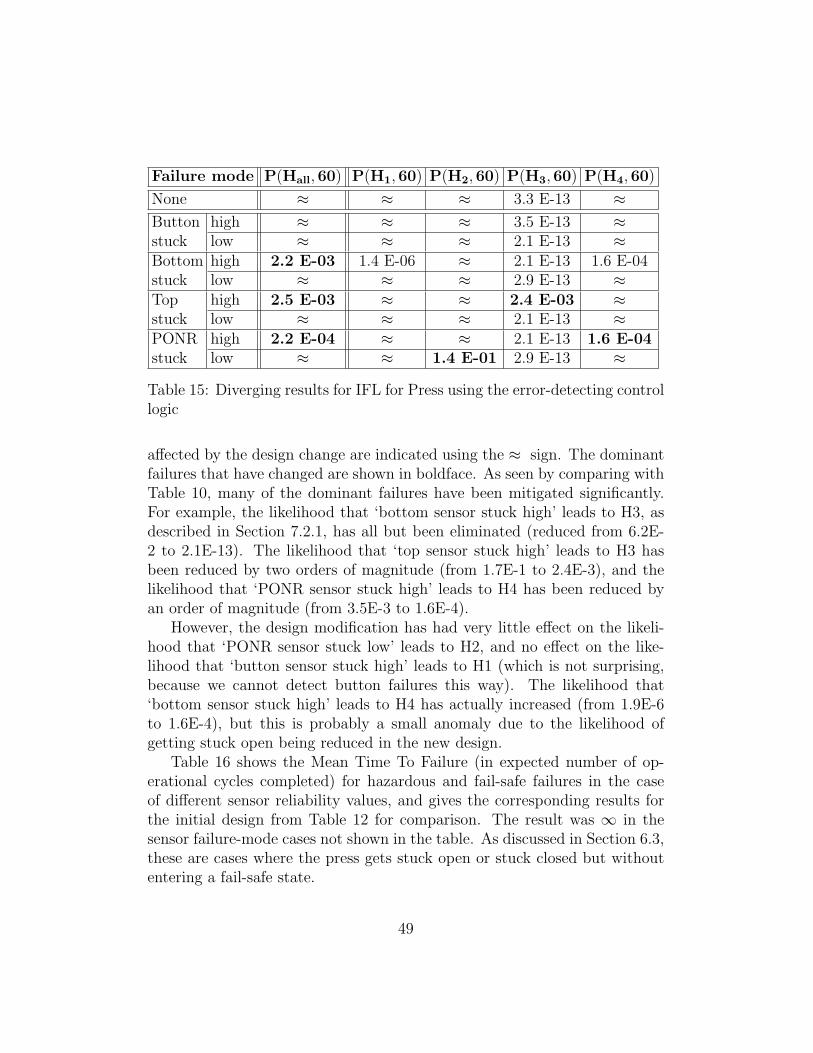
Failure mode P(Hall,60) P(H1,60) P(H2,60) P(H3,60) P(H4,60)

None ≈ ≈ ≈ 3.3 E-13 ≈

Button high ≈ ≈ ≈ 3.5 E-13 ≈stuck low ≈ ≈ ≈ 2.1 E-13 ≈Bottom high 2.2 E-03 1.4 E-06 ≈ 2.1 E-13 1.6 E-04stuck low ≈ ≈ ≈ 2.9 E-13 ≈Top high 2.5 E-03 ≈ ≈ 2.4 E-03 ≈stuck low ≈ ≈ ≈ 2.1 E-13 ≈PONR high 2.2 E-04 ≈ ≈ 2.1 E-13 1.6 E-04stuck low ≈ ≈ 1.4 E-01 2.9 E-13 ≈

Table 15: Diverging results for IFL for Press using the error-detecting controllogic

affected by the design change are indicated using the ≈ sign. The dominantfailures that have changed are shown in boldface. As seen by comparing withTable 10, many of the dominant failures have been mitigated significantly.For example, the likelihood that ‘bottom sensor stuck high’ leads to H3, asdescribed in Section 7.2.1, has all but been eliminated (reduced from 6.2E-2 to 2.1E-13). The likelihood that ‘top sensor stuck high’ leads to H3 hasbeen reduced by two orders of magnitude (from 1.7E-1 to 2.4E-3), and thelikelihood that ‘PONR sensor stuck high’ leads to H4 has been reduced byan order of magnitude (from 3.5E-3 to 1.6E-4).

However, the design modification has had very little effect on the likeli-hood that ‘PONR sensor stuck low’ leads to H2, and no effect on the like-lihood that ‘button sensor stuck high’ leads to H1 (which is not surprising,because we cannot detect button failures this way). The likelihood that‘bottom sensor stuck high’ leads to H4 has actually increased (from 1.9E-6to 1.6E-4), but this is probably a small anomaly due to the likelihood ofgetting stuck open being reduced in the new design.

Table 16 shows the Mean Time To Failure (in expected number of op-erational cycles completed) for hazardous and fail-safe failures in the caseof different sensor reliability values, and gives the corresponding results forthe initial design from Table 12 for comparison. The result was ∞ in thesensor failure-mode cases not shown in the table. As discussed in Section 6.3,these are cases where the press gets stuck open or stuck closed but withoutentering a fail-safe state.

49

Error-detecting Design Initial Design

Fault-free operation 3,511 7,581

Sensor MTTF 1 min 10 min 5 yr 1 min 10 min 5 yr

Button stuck high 0.9 9.6 3,507 0.9 10 7,580Bottom stuck high 0.9 9.9 3,507 0.9 10 7,560Top stuck high 0.9 9.9 3,507 2.8 12 7,560PONR stuck high 0.9 9.9 3,507 102 111 7,560PONR stuck low 1.4 10.4 3,507 1.9 11 7,560

Comp. time (secs) 3-6 5-7 190-216 2-7 3-7 145-211

Table 16: MTTF for Press design with and without error detection, fordifferent sensor MTTF values

As can be seen from Table 16, the risk of failures remaining hidden hasbeen significantly mitigated by the revised control logic. Both ‘top stuckhigh’ and ‘PONR stuck high’ now have expectation of being revealed withinone operational cycle. ‘PONR stuck low’ is revealed when the plunger hitsbottom, which counts as completion of an operational cycle and explains whyMTTF is greater than 1 in its case.

8.4 Summary and discussion

Modifying the control logic has had a very beneficial effect, in terms of signif-icantly reducing the risk of hidden failures, as well as significantly reducingthe likelihood of the race condition discussed in Section 7.2.1 above. Of theremaining risks, the dominant failures are ‘button sensor stuck high’ leadingto H1 (uncommanded closing) and ‘PONR sensor stuck low’ leading to H2(dangerous motor activation).

There are several different ways that the ‘button sensor stuck high’ failurecould be mitigated in the design. One way would be to reduce the severity ofthe failure by introducing a means for detecting if anyone is in the vicinity ofthe Press (such as infrared detection), and preventing closing in such a case.This would of course also involve moving the button location to outside ofthe danger zone. Another solution would be to introduce a second button,and to require that both buttons be pushed before the motor would switchoff [12]. Yet another solution would be to check that the button signal is low

50

when the plunger reaches the top and fail safe otherwise. This would involvea change to the operational procedure so that the operator was required torelease the button before the plunger reaches the top.

All of these solutions can be modelled in our framework. To demon-strate, we focus on the ‘PONR sensor stuck low’ failure mode and show howstochastic model checking can further inform design-for-safety. The nextsection investigates the effect of raising the PONR sensor above its nominalposition, in order to reduce the likelihood of the race condition that leads toH2 during fault-free operation.

9 Raising the Point of No Return sensor

The second design change we consider involves moving the PONR sensorhigher, in order to reduce the effect of the race condition that led to themotor drive being activated late (hazard H2) in fault-free operation.

9.1 Modified sensor layout

We modify the Press design so that the PONR sensor is raised higher thanthe plunger’s actual (physical) point of no return. This way, if there is a delayin activating the motor drive after a late abort, the delay will hopefully beabsorbed while the plunger is still falling above the physical PONR, andthe motor drive will be activated before the plunger reaches that point. Wecall the new PONR sensor position the operational PONR (i.e., the pointafter which it is no longer possible to abort closing) and denote its value byoPONR in what follows.

The modified design is modelled by tweaking the model from Section 8(see Figure 10). States 3, 4 and 7 are now interpreted as rising below, ris-ing above and falling above oPONR, respectively. The state “falling belowoPONR” is split into state 8 (falling below PONR) and new state 14 (fallingbetween oPONR and PONR). States 9 and 15 represent the plunger stateafter the motor drive is activated in states 7 and 14 respectively. In bothcases the plunger’s fall will be slowed – without reaching the bottom – andthen reversed, and the plunger will eventually move into state 4 as before.The hazards are defined as before.

In the PRISM code we achieve this by replacing transition

[plBelowPONR] state=7 & stateOp=2 -> FallingR1:(state’=8);

51

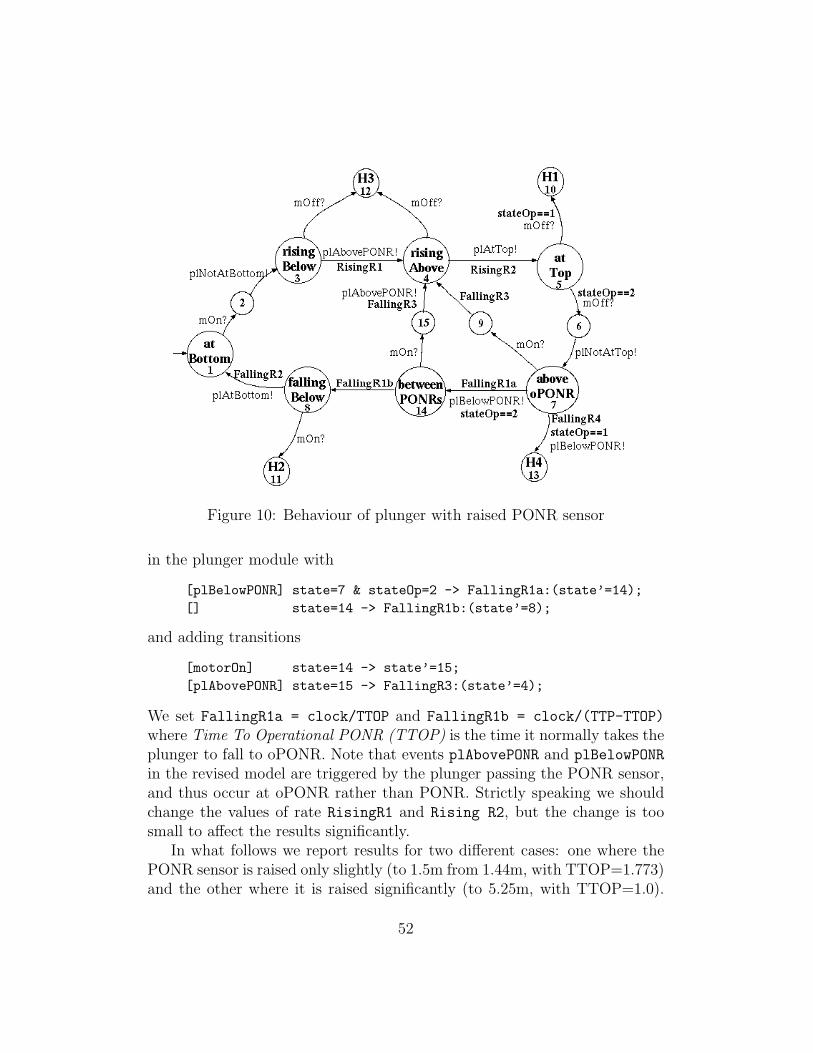
Figure 10: Behaviour of plunger with raised PONR sensor

in the plunger module with

[plBelowPONR] state=7 & stateOp=2 -> FallingR1a:(state’=14);

[] state=14 -> FallingR1b:(state’=8);

and adding transitions

[motorOn] state=14 -> state’=15;

[plAbovePONR] state=15 -> FallingR3:(state’=4);

We set FallingR1a = clock/TTOP and FallingR1b = clock/(TTP-TTOP)

where Time To Operational PONR (TTOP) is the time it normally takes theplunger to fall to oPONR. Note that events plAbovePONR and plBelowPONR

in the revised model are triggered by the plunger passing the PONR sensor,and thus occur at oPONR rather than PONR. Strictly speaking we shouldchange the values of rate RisingR1 and Rising R2, but the change is toosmall to affect the results significantly.

In what follows we report results for two different cases: one where thePONR sensor is raised only slightly (to 1.5m from 1.44m, with TTOP=1.773)and the other where it is raised significantly (to 5.25m, with TTOP=1.0).

52

P(Hall,60) P(H1,60) P(H2,60) P(H3,60) P(H4,60) Comp.time(sec)

D1 1.1 E-04 2.2 E-06 1.0 E-04 1.5 E-09 3.1 E-06 109-140

D2 1.1 E-04 2.2 E-06 1.0 E-04 3.3 E-13 3.1 E-06 244-304

D3 6.7 E-06 2.2 E-06 1.5 E-06 3.3 E-13 3.1 E-06 294-360

D4 4.1 E-06 2.2 E-06 1.4 E-07 3.3 E-13 1.8 E-06 272-334

Table 17: IFL for fault-free operation for different Press designs: (D1) initialdesign; (D2) with error detection; (D3) with PONR raised to 1.5m; (D4)with PONR raised to 5.25m

The Modelica model was used to derive the values of height of oPONR andTTOP.

9.2 Results: fault-free operation

Table 17 shows the Immediate Failure Likelihood for fault-free operation forthe revised design for the two different oPONR heights. The correspondingresults for the initial design, with and without error detection are given forcomparison. As can be seen, raising the PONR sensor reduces the IFL of dan-gerous motor activation (hazard H2) by 2-3 orders of magnitude in fault-freeoperation, without increasing the likelihood of the other hazards. Table 18also shows marked improvement in the long-term risk of H2, confirming thatraising the PONR sensor significantly reduces the likelihood of the main racecondition that gave rise to H2, without introducing new hidden failures.

9.3 With sensor failures

Although raising the PONR sensor improves safety in the fault-free case, ithas little or no effect on the IFL results in the cases where sensors may fail.The results are so similar to those in Table 15 above that they are not givenhere. In almost every case they are the same as, or slightly lower than, theresults for the error-detecting design in Section 8. The only exception is thatthe likelihood of H2 increases from 2.1E-3 to 9.1E-3 in the “bottom sensorstuck high” case when TTOP=1, which is probably due to reduced likelihood

53

Error-detecting Raised PONRTTOP=1.773

Raised PONRTTOP=1

Fault-free SensorMTTF=5yr

Fault-free SensorMTTF=5yr

Fault-free SensorMTTF=5yr

MTTF 3,511 3,507 16,404 16,304 14,882 14,799

Comp.time

82 190-216 263 598-685 242 583-656

Table 18: MTTF for three different Press designs, for fault-free and fault-prone operation

of some of the hazards that would normally precede the H2 case.Likewise, the MTTF results are almost identical to those for the error-

detecting design given in Table 16, at least for the relatively low values ofsensor reliability (1–100 mins). As seen from Table 18 above however, forhigher values of sensor reliability (in this case, 5yrs) the revised design hasa longer meant time to hazardous failure, due to reduction of risk due to therace condition around the time the plunger passes the PONR.

10 Summary and Conclusions

The paper presented an approach to risk analysis using stochastic modelchecking – or more specifically, using Continuous Time Markov Chains(CTMC) models and the PRISM tool. The approach was illustrated on theIndustrial Press case study. Although relatively simple, the Press exhibits awide range of different behaviours, including hidden failures and subtle raceconditions. We illustrated the use of quantitative analysis in support of Fail-ure Modes and Effects Analysis – in this case, the effects of sensor failureson hazardous system behaviour.

Even with such a relatively simple system, a brute force computation ofrisk over a 1 year mission lifetime proved computationally infeasible. (Thisholds true for much shorter mission times also, such as for example in thecase where a thorough inspection and test is carried out weekly.)

The main contribution of the paper was to provide computationally fea-sible methods for quantitative assessment of cause-consequence relations.Section 6 introduced two complementary analysis techniques: the first forestimating the likelihood of short-term failures (i.e., those which typically

54

manifest themselves within one operational cycle of the Press); and the sec-ond for identifying hidden failures (i.e., those which only manifest themselvesonly under specific sets of environmental conditions, which may themselvesbe comparatively rare). Together these two techniques yield valuable in-sights into which aspects of system design need more attention for safety.The short-term failure analysis method yields a quantitative relationship be-tween component failures and their consequences at system level akin to acriticality measure. The heuristic for identifying hidden failures provides agood clue as to the conditions under which the hazard will arise, althoughsubtle race conditions can sometimes confound the situation.

Our system models were based on CTMC models derived almost directlyfrom the operational concept for the system. (A Modelica simulation wasused to derive values for key rates in the model.) We demonstrated an ap-proach to injecting faults directly into a CTMC model of the system. Thishas the advantage of facilitating analysis of changes to system design simplyand quickly, and of deriving consequences of component failures directly fromthe model. This contrasts with most other forms of FMEA and criticalityanalysis, whereby models of fault propagation are constructed or generatedseparately and then have quantitative analysis performed on them. Our ap-proach is more agile and more directly aligned with the system developmentprocess, since it does not require new fault propagation models to be con-structed when the system model changes. We also included the possibilityof sensor-update timing failures (one of the sources of race conditions in ourmodel) and investigated the effect of data processing rates on hazard likeli-hood.

One downside of the approach to fault injection is that it may alter some ofthe stochastic properties of the system model being studied (cf. Section 6.2).Through careful mathematical analysis and sensitivity analysis experimentswe showed that the side-effects are relatively minor in our case study, and thatthe order of magnitude of probability estimates is not affected. It remainsan open question however to what degree this approach generalises to othersystems. We anticipate that the kind of argument given in Section 6.2 wouldtransfer to most systems with natural “cycles of operation” (such as manymanufacturing systems).

Another unanticipated difficulty we encountered was not being able toexpress some of the interesting system properties in CSL. As well as limit-ing the kinds of properties for which Immediate Failure Likelihood could becalculated, it also prevented detection of hidden failures in cases where such

55

behaviours had non-zero probability.The paper is rare in presenting a detailed study of the possibilities and

challenges of stochastic model checking for safety related systems. We showthat CTMCs are a reasonably natural way of modelling system behaviourand component failures, and that the PRISM approach has some very usefulfeatures for assisting in quantitative risk analysis.

At the same time, however, CTMCs provide challenges in representingthe timing behaviour of the system accurately. For future work it would beinteresting to investigate how other models of stochastic processes compare,such as Probabilistic Timed Automata (which separate the notion of prob-ability from that of timing) [40] or Interactive Markov Chains [41] (whichallow probabilistic transitions as well as non-deterministic choices betweentransitions). At the moment, however, the tool support for these notation isnot as advanced as that for CTMCs.

The PRISM simulator was very helpful for debugging our models and dis-covering the scenarios under which component failures led to system failures,and the fault propagation mechanisms involved. Counterexample visualiza-tion [25] is a promising technology that could improve the analyst’s ability todetermine which fault propagation mechanisms contribute most significantlyto risk. It would be interesting to see if the approach could be extended to ourmethod for calculating mean time to failure, to improve the analyst’s abil-ity to determine which fault propagation mechanisms are involved in hiddenfailures.

Acknowledgements

The authors gratefully acknowledge the assistance with PRISM and Modelicaprovided by David Parker and Adrian Pop respectively. This research wascarried out through the ARC Centre for Complex Systems with funding fromthe Australian Research Council.

References

[1] N. G. Leveson, Safeware: System Safety and Computers, Addison-Wesley, 1995.

[2] N. Storey, Safety-Critical Computer Systems, Addison-Wesley, 1996.

56

[3] International Electrotechnical Commission, Functional Safety of Elec-trical/Electronic/Programmable Electronic Safety-Related Systems, In-ternational Standard IEC 61508 (1998).

[4] International Electrotechnical Commission, Analysis Techniques for Sys-tem Reliability – Procedure for Failure Mode and Effect Analysis(FMEA), International Standard IEC 60812 (1985).

[5] E. J. Henley, H. Kumamoto, Probabilistic Risk Assessment: ReliabilityEngineering, Design, and Analysis, IEEE Press, 1992.

[6] D. Smith, Reliability, Maintainability and Risk, 7th Edition, ElsevierButterworth-Heinemann, Amsterdam, 2005.

[7] M. Kwiatkowska, G. Norman, D. Parker, PRISM: Probabilistic symbolicmodel checker, in: T. Field, P. Harrison, J. Bradley, U. Harder (Eds.),Proc. of Int. Conf. on Modelling Techniques and Tools for Computer Per-formance Evaluation (TOOLS’02), Vol. 2324 of LNCS, Springer, 2002,pp. 200–204.

[8] PRISM manual, http://www.prismmodelchecker.org/manual/.

[9] P. Fritzson, Principles of Object-Oriented Modeling and Simulation withModelica 2.1, IEEE Press, 2004.

[10] C. Baier, J.-P. Katoen, H. Hermanns, Approximate symbolic modelchecking of Continuous Time Markov Chains, in: J. Baeten, S. Mauw(Eds.), Proc. Int. Conf. on Concurrency Theory (CONCUR’99), Vol.1664 of LNCS, Springer, 1999, pp. 146–161.

[11] A. Reibman, K. Trivedi, Numerical transient analysis of Markov models,Computers & Operations Research 15 (1) (1988) 19–36.

[12] J. Hall, J. Jacob, J. McDermid, I. Toyn, Towards a z method: the twobutton press case study, Tech. rep. (May 1995).

[13] B. Atchison, P. Lindsay, Safety validation of embedded control softwareusing Z animation, in: Proc 5th IEEE Int Symp on High AssuranceSystems Engineering (HASE’00), IEEE, 2000, pp. 228–237.

57

[14] M. Kwiatkowska, G. Norman, D. Parker, Stochastic model checking, in:M. Bernardo, J. Hillston (Eds.), Formal Methods for the Design of Com-puter, Communication and Software Systems: Performance Evaluation(SFM’07), Vol. 4486 of LNCS (Tutorial Volume), Springer, 2007, pp.220–270.

[15] C. J. Price, N. Taylor, Automated multiple failure FMEA, ReliabilityEngineering and System Safety 76 (1) (2002) 1–10.

[16] B. Atchison, P. Lindsay, D. Tombs, A case study in software safetyassurance using formal methods, Tech. rep., University of Queensland,SVRC 99-31, www.itee.uq.edu.au/~pal/SVRC/tr99-31.pdf (1999).

[17] Y. Papadopoulos, D. Parker, C. Grante, A method and tool supportfor model-based semi-automated failure modes and effects analysis ofengineering designs, in: Proc. 9th Australian Workshop on Safety Criti-cal Systems and Software (SCS’04), Australian Computer Society, Inc.,2004, pp. 89–95.

[18] B. Kaiser, C. Gramlich, M. Forster, State/event fault trees – a safetyanalysis model for software-controlled systems, Reliability Engineering& System Safety 92 (11) (2007) 1521–1537.

[19] J. D. Reese, N. G. Leveson, Software deviation analysis, in: Proceedingsof the 19th International Conference on Software Engineering, ACMPress, 1997, pp. 250–261.

[20] T. Cichocki, J. Gorski, Failure mode and effect analysis for safety-criticalsystems with software components, in: F. Koornneef, M. van der Meulen(Eds.), Proc. of Int. Conf. on Computer Safety, Reliability and Security(SAFECOMP 2000), Vol. 1943 of LNCS, Springer, 2000, pp. 382–394.

[21] M. Bozzano, A. Villafiorita, Improving system reliability via modelchecking: The FSAP/NuSMV-SA safety analysis platform., in: Proc. ofInt. Conference on Computer Safety, Reliability, and Security (SAFE-COMP 2003), Vol. 2788 of LNCS, Springer, 2003, pp. 49–62.

[22] M. P. E. Heimdahl, Y. Choi, M. W. Whalen, Deviation analysis: A newuse of model checking, Automated Software Engineering 12 (3) (2005)321–347.

58

[23] L. Grunske, P. A. Lindsay, N. Yatapanage, K. Winter, An automatedfailure mode and effect analysis based on high-level design specificationwith Behavior Trees, in: J. Romijn, G. Smith, J. van de Pol (Eds.),Proc. of Int. Conf. on Integrated Formal Methods (IFM’05), Vol. 3771of LNCS, Springer, 2005, pp. 129–149.

[24] L. Grunske, R. Colvin, K. Winter, Probabilistic model-checking sup-port for FMEA, in: M. Harchol-Balter, M. Kwiatkowska, M. Telek(Eds.), Proc. of 4th Int. Conf. on the Quantitative Evaluation of Sys-Tems (QEST 2007), IEEE Computer Society Press, 2007, pp. 119–128.

[25] H. Aljazzar, M. Fischer, L. Grunske, M. Kuntz, F. Leitner, S. Leue,Safety analysis of an airbag system using probabilistic FMEA and prob-abilistic counter examples, in: Proc. of Int. Conf. on the QuantitativeEvaluation of SysTems (QEST 2009), IEEE Computer Society Press,2009.

[26] J. Elmqvist, S. Nadjm-Tehrani, Formal support for quantitative analysisof residual risks in safety-critical systems, in: Proc. High AssuranceSystems Engineering Symposium (HASE’08), IEEE Computer Society,2008, pp. 154–164.

[27] A. D. Domınguez-Garca, J. G. Kassakian, J. E. Schindall, J. J. Zinchuk,An integrated methodology for the dynamic performance and reliabilityevaluation of fault-tolerant systems, Reliability Engineering & SystemSafety 93 (11) (2008) 1628–1649.

[28] M. Bozzano, A. Cimatti, J.-P. Katoen, V. Y. Nguyen, T. Noll, M. Roveri,The COMPASS approach: Correctness, modelling and performability ofaerospace systems, in: Proc. 28th Int. Conf. on Computer Safety, Reli-ability and Security (SAFECOMP 2009), Vol. 5775 of LNCS, Springer,2009, pp. 173–186.

[29] The MRMC model checker, http://www.mrmc-tool.org/trac/.

[30] O. Hasan, N. Abbasi, S. Tahar, Formal probabilistic analysis of stuck-atfaults in reconfigurable memory arrays, in: M. Leuschel, H. Wehrheim(Eds.), Proc. of Int. Conf. on Integrated Formal Methods (IFM’07), Vol.5423 of LNCS, Springer, 2007, pp. 277–291.

59

[31] J. P. Katoen, M. Khattri, I. S. Zapreev, A Markov Reward ModelChecker, in: Proc. of Quantitative Evaluation of Systems (QEST 2005),IEEE Computer Science, 2005, pp. 243–244.

[32] H. Hermanns, J.-P. Katoen, J. Meyer-Kayser, M. Siegle, A markov chainmodel checker, in: Proc. of Int. Conf. on Tools and Algorithms for Con-struction and Analysis of Systems (TACAS 00), Vol. 1785 of LNCS,Springer-Verlag, 2000, pp. 347–362.

[33] K. Sen, M. Viswanathan, G. Agha, Statistical model checking of black-box probabilistic systems, in: Proceedings of Int. Conference on Com-puter Aided Verification (CAV ’04), Vol. 3114 of LNCS, Springer, 2004,pp. 202–215.

[34] H. L. S. Younes, R. G. Simmons, Probabilistic verification of discreteevent systems using acceptance sampling, in: Proceedings of the 14thInternational Conference on Computer Aided Verification (CAV ’02),Vol. 2404 of LNCS, Springer-Verlag, 2002, pp. 223–235.

[35] D. N. Jansen, J. Katoen, M. Oldenkamp, M. Stoelinga, I. Zapreev, Howfast and fat is your probabilistic model checker? an experimental perfor-mance comparison, in: Proceedings of the Haifa Verification Conference,Vol. 4899 of LNCS, Springer, 2007, pp. 69–85.

[36] H. Younes, M. Kwiatkowska, G. Norman, D. Parker, Numerical vs.statistical probabilistic model checking, Software Tools for TechnologyTransfer 8 (3) (2006) 216–228.

[37] D. D’Aprile, S. Donatelli, J. Sproston, CSL Model Checking for theGreatSPN Tool, in: T. Dayar, I. Korpeoglu (Eds.), Proc. of InternationalSymposium on Computer and Information Sciences, Vol. 3280 of LNCS,Springer, 2004, pp. 543–552.

[38] E. Bode, M. Herbstritt, H. Hermanns, S. Johr, T. Peikenkamp, R. Pu-lungan, R. Wimmer, B. Becker, Compositional performability evaluationfor STATEMATE, in: Proc. of Int. Conf. on the Quantitative Evaluationof SysTems (QEST 2006), IEEE Computer Society, 2006, pp. 167–178.

[39] F. Redmill, M. Chudleigh, J. Catmur, System Safety: HAZOP and Soft-ware HAZOP, John Wiley & Sons, 1999.

60

[40] M. Kwiatkowska, G. Norman, J. Sproston, F. Wang, Symbolic modelchecking for probabilistic timed automata, in: Y. Lakhnech, S. Yovine(Eds.), Proc. Joint Conference on Formal Modelling and Analysis ofTimed Systems and Formal Techniques in Real-Time and Fault TolerantSystems (FORMATS/FTRTFT’04), Vol. 3253 of LNCS, Springer, 2004,pp. 293–308.

[41] H. Hermanns, Interactive Markov Chains and the Quest for QuantifiedQuality, Vol. 2428 of LNCS, Springer, 2002.

A Modelica model of the Press

This is the model for normal (fault-free) operation of the Press:

class Press

constant Integer M = 50;

constant Integer H = 7;

constant Integer F = 850;

constant Real g = 9.81;

constant Real Fr = 6.31;

constant Real PONR = 1.44;

Boolean userpushbutton;

Real h, v;

Boolean topsensor, bottomsensor, ponrsensor, buttonsensor;

Integer motoron(start=2);

equation

der(h) = v;

when {h < 0, h > H} then reinit(v, 0); end when;

der(v) =

if motoron == 1 then

if h < H then

F/M-g + (if v>0 then -Fr else Fr)

else 0

else

if h > 0 then

-Press.g + (if v>0 then -Fr else Fr)

61

else 0;

topsensor = h >= H;

ponrsensor = h <= PONR;

bottomsensor = h <= 0;

buttonsensor = userpushbutton;

switchon = bottomsensor or

(not buttonsensor and not ponrsensor);

switchoff = topsensor and buttonsensor;

motoron = if pre(motoron) == 2 and switchon then 1

else if pre(motoron) == 1 and switchoff then 2

else pre(motoron);

end Press;

Before executing the model it is necessary to add equations that describe theoperator behaviour. For example, the case where the operator pushes thebutton after 58 sec and releases it again 3 sec later would be defined by:

userpushbutton = if 58 < time < 61 then true else false;

To model the case where for example the top sensor fails stuck high from 5sec into operation, the equation for topsesnor above would be replaced by:

topsensor = if time < 5 then h >= H else true;

B Prism model

The following modules were omitted from Section 5 in the interests of space,so are included here for completeness.

module BottomSensor

stateBS : [0..6] init 2; // High(1), Low(3)

[plAtBottom] stateBS=0 -> stateBS’=1;

[bsHigh] stateBS=1 -> stateBS’=2;

[plNotAtBottom] stateBS=2 -> stateBS’=3;

[bsLow] stateBS=3 -> stateBS’=0;

62

[bsFailsHigh] !(stateBS=4 | stateBS=5 | stateBS=6)

-> SensorFail: stateBS’=4;

[bsHigh] stateBS=4 -> stateBS’=6;

[bsFailsLow] !(stateBS=4 | stateBS=5 | stateBS=6)

-> SensorFail: stateBS’=5;

[bsLow] stateBS=5 -> stateBS’=6;

[plAtBottom] stateBS=6 -> stateBS’=6;

[plNotAtBottom] stateBS=6 -> stateBS’=6;

endmodule

module PONRSensor

statePS : [0..6] init 0; // High(1), Low(3)

[plAbovePONR] statePS=0 -> statePS’=1;

[psLow] statePS=1 -> statePS’=2;

[plBelowPONR] statePS=2 -> statePS’=3;

[psHigh] statePS=3 -> statePS’=0;

[psFailsHigh] !(statePS=4 | statePS=5 | statePS=6)

-> SensorFail: statePS’=4;

[psHigh] statePS=4 -> statePS’=6;

[psFailsLow] !(statePS=4 | statePS=5 | statePS=6)

-> SensorFail: statePS’=5;

[psLow] statePS=5 -> statePS’=6;

[plAbovePONR] statePS=6 -> statePS’=6;

[plBelowPONR] statePS=6 -> statePS’=6;

endmodule

module Button

stateB : [0..6] init 0; // pushed(1), released(3)

[pushButton] stateB=0 -> stateB’=1;

[buttonP] stateB=1 -> stateB’=2;

[releaseButton] stateB=2 -> stateB’=3;

[buttonR] stateB=3 -> stateB’=0;

[buFailsHigh] !(stateB=4 | stateB=5 | stateB=6)

-> SensorFail: stateB’=4;

[buttonP] stateB=4 -> stateB’=6;

[buFailsLow] !(stateB=4 | stateB=5 | stateB=6)

-> SensorFail: stateB’=5;

[buttonR] stateB=5 -> stateB’=6;

63

[pushButton] stateB=6 -> stateB’=6;

[releaseButton] stateB=6 -> stateB’=6;

endmodule

module Motor

stateM : [0..3] init 0; // on(1), off(3)

[turnMOn] stateM=0 -> stateM’=1;

[motorOn] stateM=1 -> stateM’=2;

[turnMOff] stateM=2 -> stateM’=3;

[motorOff] stateM=3 -> stateM’=0;

endmodule

64