![Volume 6100 Solid State Lasers XV: Technology and Devices · MODE LOCKED AND ULF LASERS Future trends and applications of ultrafast laser technology [6100-14] J. Eichenholz, M. Li,](https://static.fdocuments.net/doc/165x107/606dcab8a4d7d6735044e0f5/volume-6100-solid-state-lasers-xv-technology-and-mode-locked-and-ulf-lasers-future.jpg)
Mode Locked Fiber Lasers: Theoretical and Experimental...
146
Mode Locked Fiber Lasers: Theoretical and Experimental Developments Carsten Krogh Nielsen Department of Physics and Astronomy University of Aarhus, Denmark PhD thesis December 2006
Transcript of Mode Locked Fiber Lasers: Theoretical and Experimental...

Mode Locked Fiber Lasers:
Theoretical and Experimental
Developments
Carsten Krogh Nielsen
Department of Physics and AstronomyUniversity of Aarhus, Denmark
PhD thesisDecember 2006

This thesis is submitted to the Faculty of Science at the University ofAarhus, Denmark, in order to fulfill the requirements for obtaining thePhD degree in Physics. The studies have been carried out under thesupervision of Prof. Søren Rud Keiding.

i
Contents
Preface vAcknowledgments . . . . . . . . . . . . . . . . . . . . . . . . . . . . . . vi
List of Publications vii
1 Introduction 11.1 Mode-locked lasers . . . . . . . . . . . . . . . . . . . . . . . . . . . 11.2 Fiber lasers . . . . . . . . . . . . . . . . . . . . . . . . . . . . . . . . 21.3 Photonic Crystal Fibers . . . . . . . . . . . . . . . . . . . . . . . . . 31.4 Challenges of mode-locked fiber laser systems . . . . . . . . . . . 4
Outline of the thesis 5
2 The Nonlinear Schrodinger Equation 72.1 Introduction . . . . . . . . . . . . . . . . . . . . . . . . . . . . . . . 82.2 The nonlinear Schrodinger equation . . . . . . . . . . . . . . . . . 8
2.2.1 The nonlinear Schrodinger equation in frequency domain 112.2.2 The nonlinear Schrodinger equation in time domain: . . . 122.2.3 Nonlinearities . . . . . . . . . . . . . . . . . . . . . . . . . . 132.2.4 Two polarization states . . . . . . . . . . . . . . . . . . . . 13
2.3 Analytical solutions . . . . . . . . . . . . . . . . . . . . . . . . . . . 152.3.1 Dispersion . . . . . . . . . . . . . . . . . . . . . . . . . . . . 152.3.2 Self-phase modulation . . . . . . . . . . . . . . . . . . . . . 162.3.3 Nonlinear polarization rotation . . . . . . . . . . . . . . . . 162.3.4 Soliton . . . . . . . . . . . . . . . . . . . . . . . . . . . . . . 182.3.5 Stimulated Raman Scattering . . . . . . . . . . . . . . . . . 18
2.4 Numerical algorithm . . . . . . . . . . . . . . . . . . . . . . . . . . 19
3 Simulation of fiber lasers 213.1 Introduction . . . . . . . . . . . . . . . . . . . . . . . . . . . . . . . 223.2 Gain medium . . . . . . . . . . . . . . . . . . . . . . . . . . . . . . 22
ii CONTENTS
3.2.1 Ytterbium . . . . . . . . . . . . . . . . . . . . . . . . . . . . 233.3 Mode-locking mechanisms . . . . . . . . . . . . . . . . . . . . . . . 24
3.3.1 Nonlinear polarization rotation . . . . . . . . . . . . . . . . 243.3.2 SESAM . . . . . . . . . . . . . . . . . . . . . . . . . . . . . . 24
3.4 Cavity losses . . . . . . . . . . . . . . . . . . . . . . . . . . . . . . . 263.5 Laser cavity simulations . . . . . . . . . . . . . . . . . . . . . . . . 273.6 Numerical simulations of a 80 MHz fiber laser . . . . . . . . . . . 28
4 Characterization techniques 33Measurement of fiber dispersion . . . . . . . . . . . . . . . . . . . . . . 344.1 Introduction . . . . . . . . . . . . . . . . . . . . . . . . . . . . . . . 344.2 Experimental setup . . . . . . . . . . . . . . . . . . . . . . . . . . . 354.3 Theory . . . . . . . . . . . . . . . . . . . . . . . . . . . . . . . . . . 364.4 Dispersion measurements . . . . . . . . . . . . . . . . . . . . . . . 38Autocorrelation measurements . . . . . . . . . . . . . . . . . . . . . . . 424.5 Introduction . . . . . . . . . . . . . . . . . . . . . . . . . . . . . . . 424.6 Setup and theory . . . . . . . . . . . . . . . . . . . . . . . . . . . . 42Measurement of group birefringence . . . . . . . . . . . . . . . . . . . . 464.7 Polarization maintaining fibers . . . . . . . . . . . . . . . . . . . . 464.8 Measurement of the group birefringence . . . . . . . . . . . . . . . 474.9 Summary . . . . . . . . . . . . . . . . . . . . . . . . . . . . . . . . . 48
5 Solid core photonic bandgap fiber laser 495.1 Introduction . . . . . . . . . . . . . . . . . . . . . . . . . . . . . . . 505.2 Fiber characterization . . . . . . . . . . . . . . . . . . . . . . . . . . 515.3 Laser design . . . . . . . . . . . . . . . . . . . . . . . . . . . . . . . 525.4 Experimental results . . . . . . . . . . . . . . . . . . . . . . . . . . 545.5 Numerical simulations . . . . . . . . . . . . . . . . . . . . . . . . . 565.6 Outlook . . . . . . . . . . . . . . . . . . . . . . . . . . . . . . . . . . 585.7 Summary . . . . . . . . . . . . . . . . . . . . . . . . . . . . . . . . . 59
6 Self-similar all-polarization maintaining environmentally stable fiberlaser 616.1 Introduction . . . . . . . . . . . . . . . . . . . . . . . . . . . . . . . 626.2 Cavity design . . . . . . . . . . . . . . . . . . . . . . . . . . . . . . 646.3 Experimental results . . . . . . . . . . . . . . . . . . . . . . . . . . 66
6.3.1 Bound states . . . . . . . . . . . . . . . . . . . . . . . . . . . 686.4 Outlook . . . . . . . . . . . . . . . . . . . . . . . . . . . . . . . . . . 706.5 Summary . . . . . . . . . . . . . . . . . . . . . . . . . . . . . . . . . 70
7 Microjoule-level all polarization-maintainingfemtosecond fiber source 717.1 Introduction . . . . . . . . . . . . . . . . . . . . . . . . . . . . . . . 727.2 Theory . . . . . . . . . . . . . . . . . . . . . . . . . . . . . . . . . . 747.3 Experimental setup . . . . . . . . . . . . . . . . . . . . . . . . . . . 807.4 Experimental results . . . . . . . . . . . . . . . . . . . . . . . . . . 81

CONTENTS iii
7.5 Outlook . . . . . . . . . . . . . . . . . . . . . . . . . . . . . . . . . . 847.6 Summary . . . . . . . . . . . . . . . . . . . . . . . . . . . . . . . . . 85
8 Dispersion compensation free mode-locked fiber laser and supercon-tinuum generation 878.1 Introduction . . . . . . . . . . . . . . . . . . . . . . . . . . . . . . . 888.2 Experimental setup and results . . . . . . . . . . . . . . . . . . . . 898.3 Supercontinuum generation with a dispersion compensation free
setup. . . . . . . . . . . . . . . . . . . . . . . . . . . . . . . . . . . . 918.4 Outlook . . . . . . . . . . . . . . . . . . . . . . . . . . . . . . . . . . 938.5 Summary . . . . . . . . . . . . . . . . . . . . . . . . . . . . . . . . . 94
9 Environmentally stable low repetition rate nonlinear polarization ro-tation based fiber laser 959.1 Introduction . . . . . . . . . . . . . . . . . . . . . . . . . . . . . . . 969.2 Faraday mirror . . . . . . . . . . . . . . . . . . . . . . . . . . . . . 989.3 Proposed laser configuration . . . . . . . . . . . . . . . . . . . . . 1019.4 Startup of mode-locked lasing . . . . . . . . . . . . . . . . . . . . . 1029.5 Experimentally implemented laser configuration . . . . . . . . . . 1049.6 Experimental results . . . . . . . . . . . . . . . . . . . . . . . . . . 105
9.6.1 Amplification and supercontinuum generation . . . . . . . 1079.7 Numerical model and simulations . . . . . . . . . . . . . . . . . . 1099.8 Intra cavity Raman continuum generation . . . . . . . . . . . . . . 1149.9 All-polarization maintaining fiber laser . . . . . . . . . . . . . . . 116
9.9.1 Experimental setup and results . . . . . . . . . . . . . . . . 1189.10 Summary . . . . . . . . . . . . . . . . . . . . . . . . . . . . . . . . . 1209.11 Outlook . . . . . . . . . . . . . . . . . . . . . . . . . . . . . . . . . . 120
10 Summary and perspectives 121
Bibliography 125


v
Preface
My interest in fiber lasers began roughly one year before starting as a Ph.D. stu-dent under the supervision of Prof. Søren Rud Keiding. I attended a lecture heldby John Erland Østergaard from NKT and was intrigued by the close connec-tion between the interesting physics and real life applications related to opticalfibers. I soon became an active part of the femtogroup at The University of Aar-hus, which besides Søren also included Jakob Juul Larsen (employed by NKT,and posted in Aarhus), Jan Thøgersen (TAP at The University of Aarhus) and thethree Ph.D. students Henrik N. Paulsen, Karen M. Hilligsøe and Thomas V. An-dersen. My interest in ultrafast phenomena related to optical fibers was furtherstimulated, as we went through the book, ”Nonlinear Fiber Optics” by Agrawal[1] equation by equation. It was at that time I accepted to work on this Ph.D.project. The project is a collaboration between The University of Aarhus and theNKT-Photonics group. NKT-Photonics is a constellation of relatively small spin-off companies of which three have been relevant for this work: Koheras, CrystalFibre and NKT-Research & Innovation (NKT-Research). Koheras primarily pro-duces cw fiber laser with ultra narrow line widths. Crystal Fibre manufacturesphotonic crystal fibers. NKT-Research carries out relevant basic research to sup-port further development of the companies within the NKT-Photonics group.My primary contact has been with NKT-Research, and more specifically, ClausFriis Pedersen, although I have worked together with many others at both Ko-heras, Crystal Fibre and NKT-Research. The NKT-Photonics adventure reallytook off in the year 2000 when the NKT-owned spin-off company, Giga wassold to Intel for about 1.3 billion Euros. A large amount of this money werereinvested into fundamental research. NKT-Academy was founded and numer-ous photonics-related Ph.D. projects were initiated in Denmark and abroad. Thefocus of my Ph.D. project was the development of new mode-locked fiber lasers.Neither NKT nor the group at the University of Aarhus had any prior knowl-edge of the development of such fiber lasers, but saw the rapid development ofapplications combined with exciting technologies at NKT as an potential futureincome. The focus at NKT was further moved into applications of mode-lockedlasers at the collapse of the telecommunication market. Today the product of

vi PREFACE
perhaps biggest economic potential in NKT is their high average power super-continuum white light source, based on an amplified mode-locked fiber laserand supercontinuum generation in nonlinear photonic crystal fibers.
During the Ph.D. project, the main part of the time was spent in Aarhus.However, at numerous occasions, I also visited and worked at NKT in Birkerød.Especially the lack of a fusion splicer for polarization maintaining fibers in Aar-hus, where most of the tests on the mode-locked fiber lasers were carried out, re-sulted in many trips to NKT. In the summer of 2005, I was also fortunate enoughto gain experience from working together with Jens Limpert and Thomas Schrei-ber in their group at the University of Jena, Germany.
Acknowledgments
During my time as a Ph.D student at the University of Aarhus, I’ve had a greattime, and really enjoyed the versatile and interesting job, from which I havegained much experience - both on a theoretical, technical and personal level.There are many people that I would like to acknowledge for this time. I wouldlike to thank my supervisor, Prof. Søren Rud Keiding for giving me the possibil-ity of working with such an interesting field as fiber lasers, and giving me roomto chose my own direction within this field. Further I’ve learned from Sørenthat it is important always to pay interest to broader research fields than justones own. During my first years in the group, Jakob Juul Larsen was a greathelp in introducing me to all basic optics and ultrafast lasers, and further Jakobendured many hours of listening to my crazy ideas. Jakob functioned as exter-nal supervisor for the NKT-Academy students in Aarhus for about two yearsand was an enormous help for all of us. Jan Thøgersen has also always been agreat help in the lab, and contributed with his huge knowledge of lasers.
The femtogroup have included many people over the years, and the spiritshave always been high. This has helped in creating an pleasant and inspiringenvironment. Especially my co-worker, Thomas V. Andersen, has contributedwith his outstanding drive and work moral. Also special thanks to Jakob JuulLarsen and Victoria Birkedal for proof-reading this thesis.
I also acknowledge the helpfulness of the people at NKT Research, CrystalFibre and Koheras, and special thanks to Claus Friis Pedersen for his supportand engagement in the work in Aarhus.
Finally, I would like to thank my wife, Lene, for supporting me through outmy time as a Ph.D student, and for making it possible to have both long workinghours and a well functioning family. Especially during the last year where wegot our little daughter, and every thing had to be done by a tight schedule, shehas made a great effort in making everything run smoothly.

vii
List of Publications
Journal papers
[I] K. M. Hilligsøe, T. V. Andersen, H. N. Paulsen, C. K. Nielsen, K. Mølmer,S. R. Keiding, R. Kristensen, K. P. Hansen, J. J. Larsen, ”Supercontinuumgeneration in a photonic crystal fiber with two zero dispersion wavelengths”,Opt. Expr., 12, no. 6, 1045-1054 (2004)
[II] T. V. Andersen, K. M. Hilligsøe, C. K. Nielsen, J. Thøgersen, K. P. Hansen,S. R. Keiding, and J. J. Larsen, ”Continuous-wave wavelength conversionin a photonic crystal fiber with two zero-dispersion wavelengths”, Opt.Expr., 12, no. 17, 4113-4122 (2004)
[III] T. V. Andersen, K. M. Hilligsøe, C. K. Nielsen, J. Thøgersen, K. P. Hansen,S. R. Keiding, and J. J. Larsen, ”Continuous-wave wavelength conversionin a photonic crystal fiber with two zero-dispersion wavelengths (vol 12,pg 4113, 2004)”, Opt. Expr., 13, no. 9, 3581-3582 (2005)
[IV] C. K. Nielsen, T. V. Andersen, S. R. Keiding, ”Stability Analysis of anAll-fiber Coupled Cavity Fabry-Perot Additive Pulse Mode-Locked laser”IEEE J. Q. Electr., 41, no. 2, 198-204 (2005)
[V] C. K. Nielsen, B. Ortac, T. Schreiber, J. Limpert, R. Hohmuth, W. Richter,A. Tunnermann, ”Self-starting self-similar all-polarization maintaining Yb-doped fiber laser”, Opt. Expr., 13, no. 23, 9346-9351 (2005)
[VI] T. Schreiber, C. K. Nielsen, B. Ortac, J. Limpert, A. Tunnermann, ”µJ-Levelall-polarization-maintaining femtosecond fiber source.”, Opt. Lett., 31, no.5, 574-576 (2006)
[VII] C. K. Nielsen, K. G. Jespersen, and S. R. Keiding, ”A 158 fs 5.3 nJ fiber-lasersystem at 1 µm using photonic bandgap fibers for dispersion control andpulse compression.”, Opt. Expr., 14, no. 13, 6063-6068 (2006)
viii LIST OF PUBLICATIONS
[VIII] E. R. Andresen C. K. Nielsen, J. Thøgersen, and S. R. Keiding, ”Fiber lasersystem for CARS microscopy.”, In preparation.
[IX] C. K. Nielsen and S. R. Keiding, ”Environmentally stable all-fiber non-linear polarization rotation based mode-locked fiber laser.”, submitted toOpt. Lett.
Conference papers[X] C. K. Nielsen, T. V. Andersen, E. Riis, A. Petersson, J. Broeng ”Investi-
gations of the coupling between the core mode and cladding modes ina double clad Yb-doped photonic crystal fiber” in Proceedings of the 2004Photonics West Conference, California USA, no. 5335-26.
[XI] K. M. Hilligsøe, T. V. Andersen, H. N. Paulsen, C. K. Nielsen, K. Mølmer,S. R. Keiding, K. P. Hansen, J. J. Larsen ”Supercontinuum generation in aphotonic crystal fiber with two closely lying zero dispersion wavelengths”,OSA Trends in Optics and Photonics Series 96 A, p1567-1568
[XII] K. M. Hilligsøe, T. V. Andersen, H. N. Paulsen, C. K. Nielsen, K. Mølmer,S. R. Keiding, K. P. Hansen, J. J. Larsen ”Supercontinuum generation in aphotonic crystal fiber with two closely lying zero dispersion wavelengths”,Conference on Lasers and Electro-Optics (CLEO), 1 p2 (2004)
[XIII] C. K. Nielsen, B. Ortac, T. Schreiber, J. Limpert, R. Hohmuth, W. Richter,A. Tunnermann, ”Single pulse and bound state operation of a self-startingself-similar all-PM yb-doped fiber laser”, Proceedings of the 2006 PhotonicsWest Conference, California USA no. 6102-17
[XIV] T. Schreiber, C. K. Nielsen, B. Ortac, J. Limpert, A. Tunnermann, ”µJ-Levelall-polarization-maintaining femtosecond fiber laser.”, ASSP Jan. 2006
[XV] T. Schreiber, B. Ortac, C. K. Nielsen, J. Limpert, A. Tunnermann, ”Com-pact uJ-level all-polarization maintaining femtosecond fiber source”, Pro-ceedings of the 2006 Photonics West Conference, California USA no. 6102-11
[XVI] C. K. Nielsen, K. G. Jespersen, T. V. Andersen, S. R. Keiding, ”Disper-sion compensation with solid-core photonic bandgap fiber in an yb dopedmode-locked fiber laser”, Proceedings of the 2007 Photonics West Conference,California USA no. 6453-23
Patents[XVII] C. K. Nielsen, ”Environmentally stable all-fiber self-starting mode-locked
fiber laser”, Patent pending, EP05009990.2
[XVIII] T. Schreiber, C. K. Nielsen, B. Ortac, J. Limpert, A. Tunnermann, ”StabilerModengekoppelter Kurzpuls-Faserlaser mit polarisationserhaltenden Fasernund sattigbarem Halbleiterspiegel”, Patent pending, 05F46545-IOF

1
CHAPTER 1
Introduction
Ultrafast optics have for decades been a very rich research field, and todayshort pulsed laser systems find numerous applications in areas of fundamen-tal research as well as for medical and industrial applications. For exampleultrafast laser systems are used for time resolved studies in chemistry [2], op-tical frequency metrology [3], terahertz generation [4], two photon and CARSspectroscopy and microscopy [5], and optical coherence tomography [6]. Othermedical related applications are eye laser surgery and dentist drills [7]. In theindustry, ultrafast lasers are used for micro-machining and marking [8, 9]. Thecorner stone of ultrafast optics is the mode-locked laser, and developments ofmode-locked lasers have been a huge research field in itself.
1.1 Mode-locked lasers
Mode-locking of a laser refers to a locking of the phase relations between manyneighboring longitudinal modes of the laser cavity. Locking of such phase rela-tions enables a periodic variation in the laser output which is stable over time,and with a periodicity given by the round trip time of the cavity. If sufficientlymany longitudinal modes are locked together with only small phase differencesbetween the individual modes, it results in a short pulse which may have a sig-nificantly larger peak power than the average power of the laser. The origin ofmode-locking is best understood in the time domain. A laser in steady state isa feedback system, where the gain per round trip is balanced by the losses. If anonlinear (i.e. nonlinear in terms of optical power) element is introduced into

2 CHAPTER 1 - INTRODUCTION
the cavity, which introduces a higher loss at lower powers, the laser may favoura superposition of longitudinal modes corresponding to a short pulse with highpeak power. However, a further requirement for obtaining stable mode-lockingis that the pulse reproduces itself after one round trip (within a total phaseshifton all the longitudinal modes). The phase relations between different modes areaffected by effects such as dispersion, gain bandwidth, nonlinear phase shiftsetc. Although an infinite number of different pulses can be constructed as dif-ferent superpositions of longitudinal modes, usually only a single pulse spec-ified by its shape, duration, peak power and chirp is a stable solution of thecavity, and thus the output pulse characteristics can be designed and controlledby changing the physical parameters of the comprising laser elements.
Various mechanisms (both active and passive) exist for mode-locking lasers.For a review of active and passive mode-locking and its historical development,see e.g. reference [10]. For a review of mode-locked fiber lasers see e.g. refer-ences [11, 12], and for a more current review of fiber laser systems in general,see e.g. references [13, 14].
1.2 Fiber lasers
Traditionally, classical solid-state mode-locked lasers (i.e. lasers based on lasercrystals like e.g. the Ti:Sapphire and the Nd:YAG lasers) have dominated themarket, and in terms of reliability and long term stability these solid-state lasersare still the preferred choice. However, solid-state lasers also require stablelaboratory-like environments with optical tables and stabilized room temper-ature. Furthermore, solid-state lasers have a high power consumption, and of-ten require maintenance. If ultrafast optics are to gain grounds on much widercommercial markets, solutions to these limitations must be found.
The potential of making compact, rugged laser systems with low power con-sumption at relative low price make amplified fiber lasers a very promising al-ternative to classical solid state lasers. The key properties that make rare-earthdoped fibers attractive as laser gain media are the high single pass gain com-bined with broad gain bandwidths and excellent beam quality. These qualitiesmake fibers attractive as gain media in mode-locked lasers. The commercialmarket has been pioneered by especially one company, IMRA [15], but as themarket has grown, more companies have joined the game and developed com-mercial fiber laser products. The development of fiber lasers has initially beendriven by the massive development of telecommunication components, and formany years fiber lasers based on erbium technology have dominated the fiberlaser market. Very recently companies like e.g. IMRA and Fianium [16] havealso included fiber lasers based on ytterbium (yb) doped fibers in their assort-ment. A major reason for this recent development of fiber lasers is that fiberlasers can now be directly pumped by laser diodes. Combined with the hugeprogress and technological development of high power diode lasers, this givesa competitive edge compared to classical solid state lasers. Furthermore, the

1.3. PHOTONIC CRYSTAL FIBERS 3
development of double clad large mode area fibers for effective fiber ampli-fiers makes it possible to up-convert the spectral brightness of the multi-modediode lasers, and thus realize high average power laser outputs with excellentbeam quality. A large contribution to this development of large mode area fiberscomes from the development of photonic crystal fibers.
1.3 Photonic Crystal Fibers
Photonic crystal fibers (PCFs) are fibers with a microstructured cross section.Usually PCFs are based on a periodic arrangement of fused silica and air holesrunning parallel to the propagation-axis of the fiber, but the term PCF alsocovers fibers comprising other combinations of materials with different refrac-tive indexes. A diagram of the cross section of a typical PCF is shown in fig-ure 1.1 (left). PCFs were first proposed and demonstrated by Russell in 1996 [17].The periodic modulation of the refractive index in a PCF can result in photonicband gaps. This is similar to the creation of bandgaps in semiconductors be-cause of the periodic arrangement of atoms in a lattice. In semiconductors, elec-trons of certain energies are prohibited because of these bandgaps. In a PCF, it isphotons of certain wavelengths that are prohibited. A core in which light can beguided can be created by introducing a defect into the periodic structure. Lightof certain wavelengths is then confined to this core if the surrounding structureexhibits a bandgap at these wavelengths [18]. This class of fibers are know asphotonic bandgap (PBG) fibers.
Although PBGs have interesting features, of which some are explored in thisthesis, it is perhaps PCFs with a solid core which have had the largest impactin the field of ultrafast optics so far. Solid core PCFs guide light similarly tostandard step index fibers, but the increased flexibility in design gives PCFssome interesting properties over standard fibers. For example, if the scale of themicrostructure is comparable to the wavelength of the guided light, the diffrac-
Cladding
Core
AirSilica
Core
Inner cladding
Air cladding
Figure 1.1: Left: Diagram of the cross section of a typical solid core standardPCF. Right: Diagram of a double clad PCF.

4 CHAPTER 1 - INTRODUCTION
tion of the light penetrating into the cladding will play a dominant role on theguiding properties of the fiber. In practice this results in a strong influence onthe dispersive properties of the fiber, and hence the dispersion of the fiber canbe tailored by designing the cladding properly. This property is used in smallcore PCFs for supercontinuum generation. In chapter 8 and 9 different mode-locked laser sources are investigated for supercontinuum generation in smallcore PCFs. PBG fibers also exhibit very strong waveguide contributions to thedispersion, and in chapter 5 the use of a PBG fiber inside a mode-locked laser isinvestigated. PBG fibers with a hollow core exhibit very low nonlinearities, andin chapter 5 a hollow core PBG fiber is also used for external pulse compressionafter external amplification of the mode-locked laser.
It is possible to design single mode PCFs with much larger cores than step in-dex fibers due to the large index difference between air and silica, and the designfreedom make the creation of e.g. double clad and/or polarization maintaining(PM) fibers possible. A diagram of the cross section of a double clad PCF isshown in figure 1.1 (right). In chapter 7 amplification of a mode-locked laser tothe micro-Joule level in a large core double clad PM PCF is demonstrated.
1.4 Challenges of mode-locked fiber laser systems
Although fiber lasers have many qualities making them superior to e.g. classi-cal solid-state lasers, there are also many challenges which have to be overcome.To utilize the full potential of fibers, several things have to be fulfilled. Besidesbeing able to produce comparable pulse energies, pulse durations and averagepowers, the fiber laser system should also prove equally stable and reliable. Pri-marily the fiber laser should be environmentally stable. Environmentally stablemeans that the output from the laser is not susceptible to changing environmen-tal conditions such as changing temperatures, air convection etc. In chapter 6,8 and 9 different approaches of making environmentally stable mode-lockedlasers are presented. Furthermore, the fiber laser should preferably be imple-mented with no sections of free space optics to make it as stable, compact andcheap as possible. In chapter 9 a supercontinuum source is demonstrated whichhas no sections of free space optics and is based on an environmentally stablemode-locked laser.
Other important limitations in fiber lasers and amplifiers are the nonlineari-ties affecting the pulse due to the tight confinement and long interaction lengthsin optical fibers. In chapter 7 amplification beyond the nonlinear limit withoutstrong pulse distortions is demonstrated.

5
Outline of the thesis
In Chapter 2, the nonlinear Schrodinger equation is derived, and gives the the-oretical background for pulse propagation in optical fibers.
In Chapter 3, a numerical model for fiber laser simulations is developed.
In Chapter 4, relevant characterization techniques for mode-locked lasers areintroduced.
Chapter 5 presents a mode-locked fiber laser using solid core photonic bandgapfiber for intra cavity dispersion compensation.
Chapter 6 presents an environmentally stable mode-locked fiber laser generat-ing parabolic pulses.
Chapter 7 introduces the theory of parabolic pulse amplification and presentsthe direct amplification of parabolic pulses to power levels exceeding the non-linear limit.
Chapter 8 presents a dispersion compensation free osciallator and setup for su-percontinuum generation to high average powers.
Chapter 9 presents an environmentally stable low repetition rate mode-lockedfiber laser based on nonlinear polarization rotation.
Chapter 10 Summary and outlook.


7
CHAPTER 2
The Nonlinear SchrodingerEquation
In this chapter, the nonlinear Schrodinger equation (NLSE) will be derived. Thisequation is fundamental for the understanding of pulse propagation in opticalfibers. It forms the theoretical basis for chapter 3, where the numerical modelused for fiber laser simulations is introduced. Simplified analytical limits arealso given at the end of this chapter to introduce different concepts of pulsepropagation.

8 CHAPTER 2 - THE NONLINEAR SCHRODINGER EQUATION
2.1 Introduction
An intriguing property of light is that it can be modeled well, and its interactionwith the surroundings calculated with great accuracy. One of the most accuratemodels in physics describing the world around us, is Maxwell’s well knownequations for electromagnetic radiation. With this tool at hand, many systemsinvolving light can in principle be modeled exactly. However, the complexity ofthe system is often a limiting factor and approximations have to be introducedto obtain either simpler analytical equations or numerical calculated results thatconverge in finite time. The successful development and massive progress inthe field of laser and fiber optics is in part due to the accuracy of even sim-ple models, and the ability to predict results for complex systems, such as e.g.mode-locked lasers.
Nonlinear pulse propagation in optical fibers can be accurately modeled byone or more coupled partial differential equations which, for historical reasons,are called the nonlinear Schrodinger equations (NLSE) (Not related to the quan-tum mechanical Schrodinger equation). The NLSE have been applied in fiberoptics since the beginning of the eighties, where it was used to describe Mol-lenauer’s first experimental observations of solitons in optical fibers [19]. TheNLSE have also been applied in numerous other fields [1, 20–22]. Today it isused extensively to model pulse propagation in optical fibers [1, 23–32]. As willbe evident throughout this thesis, the development of new mode-locked fiberlasers requires numerical models, and most experimental results obtained here,have been accompanied by numerical calculations both prior, during and sub-sequent to the experiments. Furthermore, both the analytical and numericaltheory have been crucial to the initial understanding of the complicated mecha-nisms acting inside fiber lasers.
2.2 The nonlinear Schrodinger equation
The NLSE comes in a variety of different forms, depending on which approxi-mations are appropriate. The starting point of this derivation is the wave equa-tion, as obtained from Maxwell’s equations with no source terms and under theassumption (∇ · E = 0) [1]:
∇2E(r, t) =1
c2
∂2
∂t2E(r, t) + µ0
∂2
∂t2P(r, t). (2.1)
E(r, t) is the electric field and P(r, t) the induced polarization. In linear media,the induced polarization is assumed to be proportional to the electric field, butin optical fibers, where the peak intensity of especially short pulses can be veryhigh, this assumption is no longer valid, and higher order terms have to beincluded. The induced polarization can, however, be written as a sum of linearand nonlinear contributions:
P = PL + PNL = ε0χ(1) : E + ε0χ
(2) : EE + ε0χ(3) : EEE + ..., (2.2)
2.2. THE NONLINEAR SCHRODINGER EQUATION 9
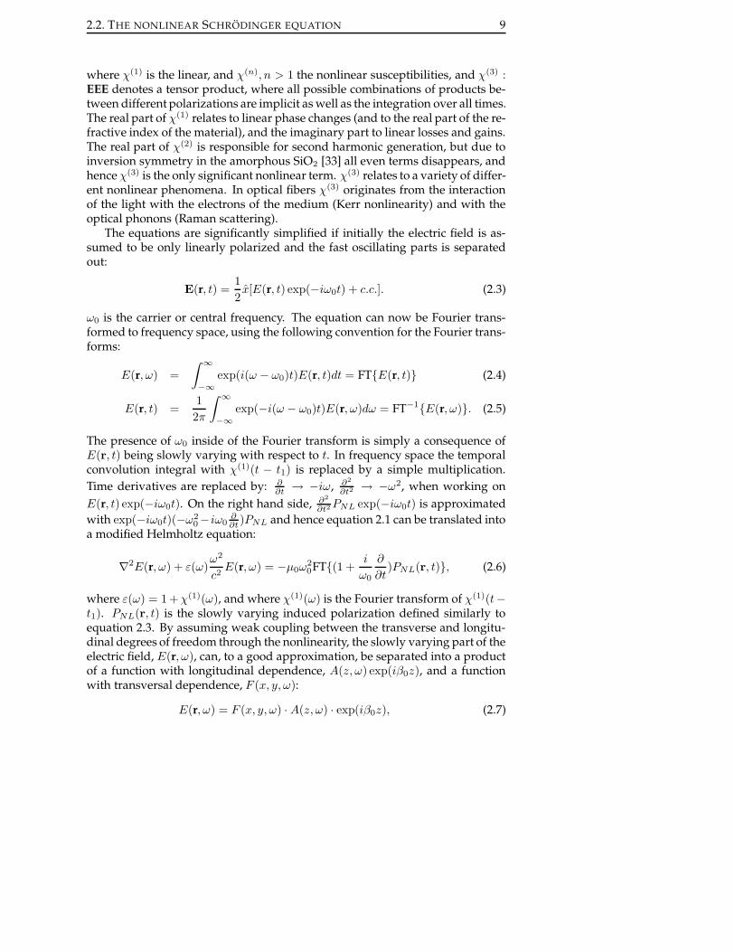
where χ(1) is the linear, and χ(n), n > 1 the nonlinear susceptibilities, and χ(3) :EEE denotes a tensor product, where all possible combinations of products be-tween different polarizations are implicit as well as the integration over all times.The real part of χ(1) relates to linear phase changes (and to the real part of the re-fractive index of the material), and the imaginary part to linear losses and gains.The real part of χ(2) is responsible for second harmonic generation, but due toinversion symmetry in the amorphous SiO2 [33] all even terms disappears, andhence χ(3) is the only significant nonlinear term. χ(3) relates to a variety of differ-ent nonlinear phenomena. In optical fibers χ(3) originates from the interactionof the light with the electrons of the medium (Kerr nonlinearity) and with theoptical phonons (Raman scattering).
The equations are significantly simplified if initially the electric field is as-sumed to be only linearly polarized and the fast oscillating parts is separatedout:
E(r, t) =1
2x[E(r, t) exp(−iω0t) + c.c.]. (2.3)
ω0 is the carrier or central frequency. The equation can now be Fourier trans-formed to frequency space, using the following convention for the Fourier trans-forms:
E(r, ω) =
∫ ∞
−∞
exp(i(ω − ω0)t)E(r, t)dt = FT{E(r, t)} (2.4)
E(r, t) =1
2π
∫ ∞
−∞
exp(−i(ω − ω0)t)E(r, ω)dω = FT−1{E(r, ω)}. (2.5)
The presence of ω0 inside of the Fourier transform is simply a consequence ofE(r, t) being slowly varying with respect to t. In frequency space the temporalconvolution integral with χ(1)(t − t1) is replaced by a simple multiplication.Time derivatives are replaced by: ∂
∂t → −iω, ∂2
∂t2 → −ω2, when working onE(r, t) exp(−iω0t). On the right hand side, ∂2
∂t2 PNL exp(−iω0t) is approximatedwith exp(−iω0t)(−ω2
0−iω0∂∂t )PNL and hence equation 2.1 can be translated into
a modified Helmholtz equation:
∇2E(r, ω) + ε(ω)ω2
c2E(r, ω) = −µ0ω
20FT{(1 +
i
ω0
∂
∂t)PNL(r, t)}, (2.6)
where ε(ω) = 1 + χ(1)(ω), and where χ(1)(ω) is the Fourier transform of χ(1)(t−t1). PNL(r, t) is the slowly varying induced polarization defined similarly toequation 2.3. By assuming weak coupling between the transverse and longitu-dinal degrees of freedom through the nonlinearity, the slowly varying part of theelectric field, E(r, ω), can, to a good approximation, be separated into a productof a function with longitudinal dependence, A(z, ω) exp(iβ0z), and a functionwith transversal dependence, F (x, y, ω):
E(r, ω) = F (x, y, ω) · A(z, ω) · exp(iβ0z), (2.7)

10 CHAPTER 2 - THE NONLINEAR SCHRODINGER EQUATION
where A(z, ω) can further be assumed to be a slowly varying function of z un-der the Slowly Varying Envelope approximation (SVEA). F (x, y, ω) is assumedto be normalized:
∫∞
−∞ dxdyF (x, y, ω) = 1. An important assumption for thederivation of the NLSE is that F (x, y, ω) is independent of ω so that it can bemoved outside the Fourier transform:
E(r, t) = FT−1{F (x, y, ω) · A(z, ω) · exp(iβ0z)} (2.8)= F (x, y) · exp(iβ0z) ·A(z, t), (2.9)
where A(z, t) = FT−1{A(z, ω)}. This assumption corresponds to the assumptionof a wavelength independent mode-field diameter (MFD). However, the MFDmay vary considerably on a wavelength scale of ∼ 100 nm. Hence this assump-tion is reasonable only for pulse widths smaller than this. β0 is the wave number,chosen so that: β0 ≡ β(ω0), where β(ω) is found below. The Helmholtz equa-tion, equation 2.6, can then be separated into equations of independent trans-verse and longitudinal parts:
(∂2
∂x2+
∂2
∂y2)F (x, y) + ε(ω)
ω2
c2F (x, y) = β2F (x, y) (2.10)
F (x, y)(2iβ0∂
∂z+ 2β0(β − β0))A(z, ω) =
µ0ω20FT{(1 +
i
ω0
∂
∂t)PNL(r, t)}, (2.11)
where the SVEA approximation was used to neglect a second derivative term:∂2
∂z2 A(z, ω), and (β2 − β20) was approximated with 2β0(β − β0) in equation 2.11.
Both these approximations are justified as long as ω − ω0 << ω [1]. In equation2.10 β = β(ω) is the eigenvalue and F (x, y) the eigenfunctions of the transversefield distribution, which have to be found for a given fiber geometry and fibercharacteristics. F (x, y) is usually refered to as modes. For step-index fibersF (x, y) is a superposition of Bessel and Neuman functions. However, for mostsingle mode fibers a Gaussian approximation of F (x, y) is adequate. A fiber iscalled multi mode if more than one solution to equation 2.10 exists, but as onlysingle mode fibers are treated in this thesis, the NLSE will only be derived forthis case. Higher order transverse modes are usually unwanted in fiber opticsand especially when short pulses are involved. They can lower the brightness,and lead to pulse break up due to different propagation velocities of the differentmodes. The waveguide contribution to the propagation constant, β(ω), alsoenters through equation 2.10.
In most dielectric materials, and also in optical fibers, the real part of ε(ω)dominates and even in high loss and high gain fibers, the imaginary part is onlya small perturbation. Hence, the (real) refractive index, n, can be introduced as:
ε(ω) = (n(ω) + ∆n(ω))2 ≈ n(ω)2 + 2n(ω)∆n(ω), (2.12)

2.2. THE NONLINEAR SCHRODINGER EQUATION 11
where the imaginary part is included as a small perturbation in ∆n(ω):
∆n(ω) =i(α(ω)− g(ω))c
2ω. (2.13)
α(ω) represents the linear power loss and g(ω) the linear power gain (in unitsof m−1). In first-order perturbation theory ∆n(ω) does not affect the transversefield distribution, F (x, y), but only the eigenvalues. Hence β(ω) in equation 2.11is replaced with β(ω) + ∆β(ω), where:
∆β(ω) =ω
c
∫ ∫
∆n(ω)|F (x, y)|2dxdy
= iα(ω)
2− i
g(ω)
2. (2.14)
The induced nonlinear polarization can be approximated by:
PNL(r, t) = −ε02n2n(ω0)E(r, t)
∫ ∞
−∞
R(t− t1)|E(r, t1)|2dt1 (2.15)
where only terms oscillating with ω0 have been maintained. Terms oscillatingwith 3ω0 have been neglected, as these correspond to third harmonic generationand require phase matching which is usually not present in the fiber. Equiva-lently one could say, that these terms oscillate so fast compared to the slowlyvarying terms, that their contributions average out. The nonlinear refractive in-dex, n2, has been introduced. n2 is proportional to the real part of χ(3), andif A(z, ω) is chosen to be normalized to units of W1/2, n2 is in the order of2 − 3 · 10−20 m2/W in standard silica fibers, depending on the doping [1]. Theimaginary part of χ(3) relates to two photon absorption and emission, and is alsonegligible. R(t− t1) is the nonlinear response function normalized in a mannersimilar to the delta function, i.e.,
∫∞
−∞R(t − t1)dt1 = 1. If only the interactions
with the electrons are included, R(t − t1) can be approximated by a delta func-tion, δ(t− t1), as the electronic response of the material is almost instantaneous.This approximation is valid in the limit where the pulse spectrum correspondsto a transform limited pulse with a duration above ∼ 1 ps [1]. In short mode-locked fiber lasers, this is also a reasonable assumption as stimulated Ramanscattering is usually not present in the output, but as shown in chapter 9 this isnot always the case. Also, if soliton dynamics are involved inside the laser, theRaman contribution to χ(3) is highly relevant, as especially a soliton can experi-ence a significant red shift over a short length of fiber due to this effect [1, 34].With these assumptions, the NLSE in frequency domain can now be derived:
2.2.1 The nonlinear Schrodinger equation in frequency domain
Using again the approximation of equation 2.9, the transverse dependence ofequation 2.11 can be integrated out by multiplying with F ∗(x, y), and integrat-
12 CHAPTER 2 - THE NONLINEAR SCHRODINGER EQUATION
ing over x and y:
∂
∂zA(z, ω) = i(β − β0)A(z, ω)− α(ω)
2A(z, ω) +
g(ω)
2A(z, ω)
+iγFT{(1 +i
ω0
∂
∂t)A(z, t)
∫ ∞
−∞
R(t− t1)|A(z, t1)|2dt1}, (2.16)
where the nonlinear coefficient, γ = ω0n2
cAeff, has been introduced, and where:
Aeff =1
∫ ∫
dxdy|F (x, y)|4 (2.17)
is the effective area of the fiber. Equation 2.16 is the NLSE in frequency space in-cluding the self-steepening and shock formation term, i
ω0
∂∂t , and the full Raman
integral. If the self-steepening term is neglected, and R(t− t1) approximated bya delta function, the NLSE in frequency domain reduces to:
∂
∂zA(z, ω) = iβ(ω)′A(z, ω)− α(ω)
2A(z, ω) +
g(ω)
2A(z, ω)
+iγFT{|A(z, t)|2A(z, t)}. (2.18)
where A(z, t) = FT−1{A(z, ω)}, and where the propagation has been expandedin a Taylor series:
β(ω)′ =n(ω)ω
c− β0(ω0)− β1(ω0)(ω − ω0)
=∑
m>1
1
m!βm(ω − ω0)
m; βm =∂mβ
∂ωm
∣
∣
∣
ω=ω0
=1
2β2(ω0)(ω − ω0)
2 +1
6β3(ω0)(ω − ω0)
3 + ... (2.19)
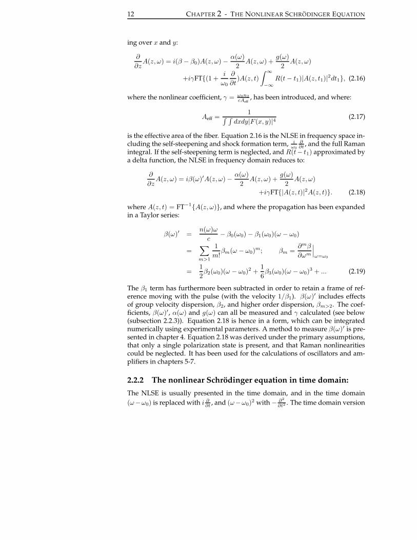
The β1 term has furthermore been subtracted in order to retain a frame of ref-erence moving with the pulse (with the velocity 1/β1). β(ω)′ includes effectsof group velocity dispersion, β2, and higher order dispersion, βm>2. The coef-ficients, β(ω)′, α(ω) and g(ω) can all be measured and γ calculated (see below(subsection 2.2.3)). Equation 2.18 is hence in a form, which can be integratednumerically using experimental parameters. A method to measure β(ω)′ is pre-sented in chapter 4. Equation 2.18 was derived under the primary assumptions,that only a single polarization state is present, and that Raman nonlinearitiescould be neglected. It has been used for the calculations of oscillators and am-plifiers in chapters 5-7.
2.2.2 The nonlinear Schrodinger equation in time domain:
The NLSE is usually presented in the time domain, and in the time domain(ω−ω0) is replaced with i ∂
∂t , and (ω−ω0)2 with− ∂2
∂t2 . The time domain version
2.2. THE NONLINEAR SCHRODINGER EQUATION 13
of the NLSE can now be found by simply Fourier transforming equation 2.18:
∂
∂zA(z, t) = −i
β2
2
∂2
∂t2A(z, t)− α0
2A(z, t) +
g0
2A(z, t)
+iγ|A(z, t)|2A(z, t), (2.20)
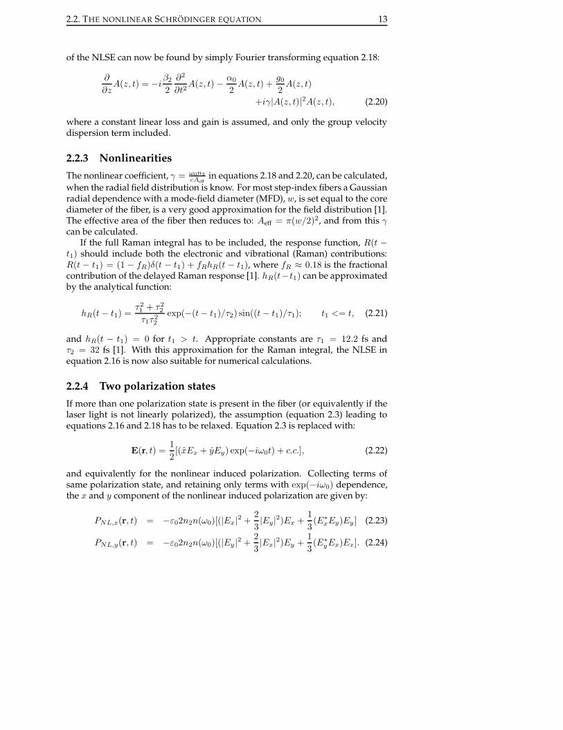
where a constant linear loss and gain is assumed, and only the group velocitydispersion term included.
2.2.3 NonlinearitiesThe nonlinear coefficient, γ = ω0n2
cAeffin equations 2.18 and 2.20, can be calculated,
when the radial field distribution is know. For most step-index fibers a Gaussianradial dependence with a mode-field diameter (MFD), w, is set equal to the corediameter of the fiber, is a very good approximation for the field distribution [1].The effective area of the fiber then reduces to: Aeff = π(w/2)2, and from this γcan be calculated.
If the full Raman integral has to be included, the response function, R(t −t1) should include both the electronic and vibrational (Raman) contributions:R(t − t1) = (1 − fR)δ(t − t1) + fRhR(t − t1), where fR ≈ 0.18 is the fractionalcontribution of the delayed Raman response [1]. hR(t− t1) can be approximatedby the analytical function:
hR(t− t1) =τ21 + τ2
2
τ1τ22
exp(−(t− t1)/τ2) sin((t− t1)/τ1); t1 <= t, (2.21)
and hR(t − t1) = 0 for t1 > t. Appropriate constants are τ1 = 12.2 fs andτ2 = 32 fs [1]. With this approximation for the Raman integral, the NLSE inequation 2.16 is now also suitable for numerical calculations.
2.2.4 Two polarization statesIf more than one polarization state is present in the fiber (or equivalently if thelaser light is not linearly polarized), the assumption (equation 2.3) leading toequations 2.16 and 2.18 has to be relaxed. Equation 2.3 is replaced with:
E(r, t) =1
2[(xEx + yEy) exp(−iω0t) + c.c.], (2.22)
and equivalently for the nonlinear induced polarization. Collecting terms ofsame polarization state, and retaining only terms with exp(−iω0) dependence,the x and y component of the nonlinear induced polarization are given by:
PNL,x(r, t) = −ε02n2n(ω0)[(|Ex|2 +2
3|Ey|2)Ex +
1
3(E∗xEy)Ey ] (2.23)
PNL,y(r, t) = −ε02n2n(ω0)[(|Ey |2 +2
3|Ex|2)Ey +
1
3(E∗yEx)Ex]. (2.24)

14 CHAPTER 2 - THE NONLINEAR SCHRODINGER EQUATION
Here the response function, R(t− t1), has also been approximated with a deltafunction. Two coupled equations for the slowly varying parts of Ex and Ey cannow be derived in a similar manner as above:
∂
∂zAx(ω) = iβ(ω)′Ax(ω) + i
∆β1
2(ω − ω0)Ax(ω)− α(ω)
2Ax(ω) +
g(ω)
2Ax(ω)
+iγFT{(|Ax(t)|2 +2
3|Ay(t)|2)Ax(t) +
i
3Ax(t)∗Ay(t)2 exp(−2i∆β0z)} (2.25)
∂
∂zAy(ω) = iβ(ω)′Ay(ω)− i
∆β1
2(ω − ω0)Ay(ω)− α(ω)
2Ay(ω) +
g(ω)
2Ay(ω)
+iγFT{(|Ay(t)|2 +2
3|Ax(t)|2)Ay(t) +
i
3Ay(t)∗Ax(t)2 exp(2i∆β0z)}, (2.26)
where ∆β0 = β0,x − β0,y = ωc ∆n. and where ∆β1 = β1,x − β1,y =
∆ng
c . ∆nis the (phase) birefringence of the fiber, and ∆ng is the group birefringence. Inchapter 4 a method to measure the group birefringence is introduced. A frameof reference moving at the average velocity 2/(β1,x +β1,y) have been chosen (in-formation contained in the terms ±i∆β1
2 ), and hence the x polarized field moveswith a relative velocity of 2/∆β1 compared to the frame of reference, and the ypolarized field moves with a relative velocity of−2/∆β1. The coefficients, β(ω)′,α(ω) and g(ω) can usually be assumed to be polarization independent. The in-teraction between the two different polarization states (and hence the differenceto two separate NLSE for a single polarization state) is in the nonlinear term.
Two limits are interesting in this thesis: Highly birefringent fibers and non-birefringent fibers. For the later case, ∆β0 = 0 and ∆β1 = 0. To eliminate theA∗xA2
y and A∗yA2x terms in equations 2.25 and 2.26, the polarization representa-
tion can be changed from linear to circular, by introducing:
A+ = (Ax + iAy)/√
2, A− = (Ax − iAy)/√
2. (2.27)
Equations 2.25 and 2.26 then reduce to:
∂
∂zA+(ω) = iβ(ω)′A+(ω)− α(ω)
2A+(ω) +
g(ω)
2A+(ω)
+i2γ
3FT{(|A+(t)|2 + 2|A−(t)|2)A+(t)} (2.28)
∂
∂zA−(ω) = iβ(ω)′A−(ω)− α(ω)
2A−(ω) +
g(ω)
2A−(ω)
+i2γ
3FT{(|A−(t)|2 + 2|A+(t)|2)A−(t)}. (2.29)
In the high birefringence case, the exp(−2i∆β0z) and exp(2i∆β0z) terms oscil-late so rapidly, that they can be neglected. It is hence most favourable to remainthe linear polarization representation. Although the equations are solved in thefrequency domain, for clarity, the time domain version of equations 2.25-2.29are:

2.3. ANALYTICAL SOLUTIONS 15
High birefringence approximation:
∂Ax
∂z= −∆β1
2
∂Ax
∂t− i
β2
2
∂2Ax
∂t2+
β3
3
∂3Ax
∂t3
+ iγ(|Ax|2 +2
3|Ay|2)Ax + (
g0
2− α0
2)Ax (2.30)
∂Ay
∂z= +
∆β1
2
∂Ay
∂t− i
β2
2
∂2Ay
∂t2+
β3
3
∂3Ay
∂t3
+ iγ(|Ay|2 +2
3|Ax|2)Ay + (
g0
2− α0
2)Ay , (2.31)
Non-birefringence approximation:
∂A+
∂z= −i
β2
2
∂2A+
∂t2+
β3
3
∂3A+
∂t3+ i
∆β
2A−
+ iγ2
3(|A+|2 + 2|A−|2)A+ + (
g0
2− α0
2)A+ (2.32)
∂A−∂z
= −iβ2
2
∂2A−∂t2
+β3
3
∂3A−∂t3
+ i∆β
2A+
+ iγ2
3(|A−|2 + 2|A+|2)A− + (
g0
2− α0
2)A−, (2.33)
A NLSE for two polarization directions is used in the model of the laserpresented in chapter 9, and the two limits are relevant for modeling nonlin-ear polarization rotation (see below (subsection 2.3.3)) in polarization maintain-ing (PM) fibers (High-birefringence approximation) and non-PM fibers (Non-birefringence approximation). In the derivation of the NLSE for the two polari-zation directions, Raman contributions were not included in the nonlinearities.A NLSE for two polarization directions and with the inclusion of the Ramanterms can be found in references [35–40], and information about the coefficientsin reference [41].
2.3 Analytical solutions
To understand the physics behind the NLSE, it is beneficial to look at some lim-iting cases, which can be calculated analytically.
2.3.1 Dispersion
To illustrate the effects of dispersion on a pulse, a simple analytical calculationcan be done if all other terms but the group velocity dispersion are neglected:
∂
∂zA(z, ω) = i
β2
2(ω − ω0)
2A(z, ω),

16 CHAPTER 2 - THE NONLINEAR SCHRODINGER EQUATION
For an initial Gaussian pulse with no chirp and FWHM temporal duration, t0,the field can be written as:
A(0, t) = A0 exp(
− 2 ln(2)( t
t0
)2)
(2.34)
After propagation through a fiber of length, L, and with group velocity dis-persion, β2, the output can analytically be calculated to be a chirped Gaussianpulse:
A(L, t) = A0 exp(
− 2 ln(2)1 + iC
1 + C2
( t
t0
)2)
, (2.35)
where the C is given by: C = 2β2L2 ln(2)
t22
. The chirp of the pulse, c(t) = − ∂φ∂t ,
where φ is the phase, is then given by c(t) = 4 ln(2)Ct/t20, and is linear in t. TheFWHM temporal pulse duration has now increased to:
√1 + C2t0. Spectrally
nothing has happened (to the power spectrum), as only a quadratic phase hasbeen added:
A(L, ω) = exp(iβ2
2L(ω − ω0)
2)A(0, ω),
2.3.2 Self-phase modulationIf nonlinearities are also present, the pulse also obtains a intensity dependentand hence nonlinear phase. This is referred to as self-phase modulation (SPM).To illustrate the effects of SPM, all other terms are again neglected:
∂
∂zA(z, t) = iγ|A(z, t)|2A(z, t).
This equation can also be integrated analytically to give:
A(L, t) = exp(iγL|A(0, t)|2)A(0, t).
If the initial pulse is again assumed to be an unchirped Gaussian pulse (equa-tion 2.34), then the chirp of the pulse has a nonlinear temporal dependence, andwhereas nothing has happened to the temporal shape of the pulse, the spectrumis now no longer Gaussian, but has spectrally broadened. Figure 2.1 shows thepure SPM spectral broadening of a 100 fs Gaussian pulse centered at 1030 nm.As shown in chapter 6 and 7, a special class of pulses (parabolic pulses), only ac-quires a linear chirp in the presence of nonlinearities, and interesting propertiesof parabolic pulses are investigated in these chapters.
2.3.3 Nonlinear polarization rotationIf a general elliptically polarized pulse is launched into a fiber where nonlinear-ities are present, it will experience a nonlinear polarization rotation (NPR). To

2.3. ANALYTICAL SOLUTIONS 17
0
0.2
0.4
0.6
0.8
1
800 900 1000 1100 1200 1300
Pow
er /
a.u.
Wavelength / nm
φNL = 0 πφNL = 2 πφNL = 4 πφNL = 6 π
Figure 2.1: Pure SPM spectral broadening of a 100 fs Gaussian pulse centered at1030 nm. The spectra are calculated at peak nonlinear phase shifts of 0, 2, 4 and6 π.
illustrate this, only the nonlinear terms of the NLSE for two polarization direc-tions and in the non-birefringence approximation are maintained and all otherterms neglected:
∂A+
∂z= iγ
2
3(|A+|2 + 2|A−|2)A+
∂A−∂z
= iγ2
3(|A−|2 + 2|A+|2)A−.
These equations can also be integrated analytically to yield:
[ A+(L)A−(L)
]
= exp(i1
2(Φ+ + Φ−))
[ cos(Φ+−Φ−
2 ) − sin(Φ+−Φ−
2 )
sin(Φ+−Φ−
2 ) cos(Φ+−Φ−
2 )
][ A+(0)A−(0)
]
,
where:
Φ+ =2
3γ(|A+(0)|2 + 2|A−(0)|2) (2.36)
Φ− =2
3γ(|A−(0)|2 + 2|A+(0)|2) (2.37)
Φ+ − Φ− =2
3γ(|A−(0)|2 − |A+(0)|2), (2.38)
and hence the polarization state rotates with an angle of (Φ+ − Φ−)/2. Noticethat this angle is zero if the light is initially linearly polarized, as |A−(0)|2 =|A+(0)|2, and hence Φ+ − Φ− = 0. Also if the light is circular polarized, thepolarization state is maintained.

18 CHAPTER 2 - THE NONLINEAR SCHRODINGER EQUATION
2.3.4 Soliton
The soliton plays an important role in many areas of fiber optics, and as solitonsare mentioned several times in this thesis, its analytical form is given here. Thefundamental soliton is a solution of the simple NLSE:
∂
∂zA(z, t) = −i
β2
2
∂2
∂t2A(z, t) + iγ|A(z, t)|2A(z, t),
which preserves both its temporal and spectral shape, as it propagates in thefiber. The fundamental soliton is found in the anomalous dispersion regime(β2 < 0), and is characterized by a very characteristic sech shape:
|A(z, t)| =( |β2|
γt20
)1/2
sech( t
t0
)
,
and occurs when nonlinearities are exactly balanced by dispersion in the fiber.
2.3.5 Stimulated Raman Scattering
The Raman integral in the NLSE originates from inelastic scattering on the opti-cal phonons in the fiber. On the creation of an optical phonon, the photon energyis reduced, and hence the wavelength of the photon increases. This effect effec-tively corresponds to a gain on the red side of the pulse, and the peak of thisRaman gain is centered at about 13.2 THz from the central wavelength of thepulse. Starting from noise a new pulse will start to build up at this wavelength,and will eventually drain most of the energy from the original pulse. This isreferred to as Stimulated Raman Scattering (SRS). The created pulse, called the1th Stokes pulse will, when its peak power has increased sufficiently, start tocreate a new pulse, called the 2nd Stokes pulse, and so on. Chapter 9 presents anice example of SRS. As the onset of SRS is a stochastic process, which dependson the peak power, fiber length, linear losses, etc., a threshold peak power canbe calculated below which SRS can be neglected [1]:
P thpeak =
16Aeff
gRL
αL
1− e−αL.
Aeff is the effective area of the fiber, gR, is the peak Raman-gain (gR ≈ 10−13 m/W),α is the power loss per unit length and L is the length of the fiber.
In anomalous dispersive fibers where a soliton can be created, the mecha-nisms creating the soliton will try to maintain the solitonic shape of the pulseeven in the presence of the Raman gain. The result is a soliton which grad-ually redshifts toward higher wavelengths instead of generating a 1th stokespulse [1, 34]. As the soliton gradually looses energy, it compensates by chang-ing its width, while maintaining its sech shape.

2.4. NUMERICAL ALGORITHM 19
2.4 Numerical algorithm
To reduce computational workload it is worth noticing that dω in the Fourierintegral in equation 2.5 without loss of generality can be replaced by d(ω − ω0),and hence a new variable, ω1 = ω − ω0 can be introduced. Equations 2.4 and2.5 are now mathematically on the standard Fourier integral form, and standardfast Fourier algorithms can be used. All fields in the frequency space can nowbe centered at ω1 = 0, and restricted to the range where the pulse spectrumexists. Equivalently, the fields in the temporal space can be centered at t = 0,and extended only to a range containing the temporal pulse.


21
CHAPTER 3
Simulation of fiber lasers
A numerical model for fiber laser simulations is presented. The model is basedon the nonlinear Schrodinger equation (NLSE) which was derived in chapter 2.The model further comprises effects of saturable gain, nonlinear losses and cav-ity losses in general, which are described in this chapter. The cavity is modeledas a sequence of different elements. In the simulations, a pulse is iterated fromnoise over many round trips until a steady solution is reached.

22 CHAPTER 3 - SIMULATION OF FIBER LASERS
3.1 Introduction
The theory behind mode-locked lasers is well established. For classical solidstate and dye lasers advanced analytical theories exists, and the master equa-tion developed by Haus is perhaps one of the most successful models describingmany types of mode-locked lasers [10, 42–46]. However, as the analytical theoryis based on a linearization of the effect of all cavity elements on the pulse, thetheory is only adequate if these effects are weak on each pass. In fiber lasers ingeneral, and for the lasers in this thesis in particular, this is not the case, andhence more advance models based on numerical calculations have to be used.The models used in this thesis is based on solving the NLSE numerically. Thereare however additional effects which have to be included for adequate descrip-tions of a mode-locked fiber laser. First of all, a more advanced description of thegain medium is needed. Second, a model of the mode-locking mechanism hasto be included, and finally cavity losses also has to be taken into account. Theseeffects are described below, before an outline of a laser simulation is given. Asan example simulations of an 80 MHz mode-locked fiber laser are presented.
3.2 Gain medium
The linear gain factor, g(ω), in the NLSE represents a small signal gain and, ifg(ω) is constant as function of z, the power increases exponentially as exp(gz).However in real fibers, where a gain can be introduced by doping the fiber withappropriate optical active atoms, like e.g. rare earth atoms (Erbium, Ytterbium,Thulium, Neodymium, etc.), and by creating a population inversion by meansof optical pumping, the gain experienced by a pulse depends on the intensityof the pulse. At increasing pulse intensities, the gain saturates. As the pulseduration as well as the round trip time is usually much shorter than the relax-ation time of the excited states in the rare earth atoms, the population inver-sion in steady state operation only saturates as function of the average powerof the pulse train. The lifetime of the excited state is ∼ 10 ms in erbium and∼ 1 ms in ytterbium. If the fiber is pumped from one end, this further cre-ates a nonuniform distribution of population inversion in the fiber due to thegradual absorption of the pump light. This nonuniform population inversioncan be calculated using rate equations for the average power distribution in thefiber [47–52]. However, to simplify the numerical model and reduce computa-tion time, this z dependence can to a good approximation be neglected if thedoped fiber is really short. Hence the gain can be modeled by replacing:
g(ω)/2→ g(ω)/2
1 + Pave(z)Psat
, (3.1)
where Psat is the saturation power and Pave is the average power of the pulsetrain in the doped fiber. In linear cavities, the signal power enters the gain

3.2. GAIN MEDIUM 23
medium from both sides, and hence the average power in the gain mediumshould be calculated as:
Pave(z) = frep
∫ TR/2
−TR/2
|A(z, t)|2dt + P←ave(z) (3.2)
where frep is the repetition rate and TR = 1/frep the round trip time. P←ave(z)is the average power of the signal propagating in the opposite direction of thedoped fiber. The inclusion of the average power from the signal propagatingin the opposite direction is especially important if the gain fiber is located in afiber laser where the loss on one side of the gain medium is much larger thanon the other side. This is the case in many of the oscillators presented in thisthesis. The result is a smaller amplification of the signal coming from the highloss side, due to saturation of the gain medium from the signal coming from thelow loss side.
3.2.1 Ytterbium
All fiber lasers presented in this thesis are based on ytterbium doped fibers asthe gain medium. Ytterbium has a very simple structure, and can be describedas a 2 level system (see figure 3.1 (right)), where there is no excited state ab-sorption of neither the pump nor the laser wavelengths [47, 51]. Figure 3.1 (left)shows the absorption and emission cross sections of ytterbium.
0
0.5
1
1.5
2
2.5
3
850 900 950 1000 1050 1100 1150 1200
Cro
ss s
ectio
n / p
m2
Wavelength / nm
EmissionAbsorption F
5/2
2
F7/2
2
σsa
σpa
σpe
σse
Figure 3.1: Left: The absorption and emission cross section for Yb3+-doped silica[51]. Right: Energy band diagrams of ytterbium. (σpa, σpe, σsa, σse: pump andsignal absorption and emission cross sections respectively.)
There are several reasons why ytterbium is an ideal candidate for mode-locked fiber lasers. Ytterbium has a high absorption at 976 nm, and for thiswavelength there have been a large development of both single mode fiberpigtailed diode pump lasers and high power diode pump lasers (Single modepump lasers at 976 nm have primarily been developed for use with Erbium inthe telecommunication industry). Ytterbium further has a high quantum effi-ciency (∼ 95 %), as the lasing band is very close to the pump wavelength. Very

24 CHAPTER 3 - SIMULATION OF FIBER LASERS
high doping concentrations are possible in ytterbium doped fibers, enablingvery high single pass gains and high slope efficiencies (proportionality factorbetween output power and pump power) of up to ∼ 80 %. This simplifies real-izations of high efficiency fiber amplifiers [53], [VI], and hence necessary pulseenergies and average powers for most applications are more easily reached withytterbium based fiber laser systems. As seen in figure 3.1 (left), the emissionband is also very broad and is hence cable of supporting very short pulses [54].The gain of an ytterbium doped fiber can be well modeled by a Gaussian func-tion with FWHM of ∼40 nm and with a central wavelength at 1030 nm.
3.3 Mode-locking mechanisms
Beside the ability to model dispersion, gain, losses, nonlinearities, etc. in fibers,one important component is still missing to model mode-locked lasers. Thisis the nonlinear component used to make mode-locked lasing more favourablethan cw lasing. For a laser to favour lasing in a mode with short pulses, anelement or a combination of elements have to be present in the cavity, whichintroduces a higher loss at low power, so that a short pulse with higher peakpower experiences a lower loss.
3.3.1 Nonlinear polarization rotation
One widely used possibility is to use nonlinear polarization rotation (NPR) inconjunction with a polarizer [10, 24, 42, 54–59]. By controlling the polarizationstate into a fiber with e.g. a set of wave-plates, the transmission through a po-larizer on the other side of the fiber will be power dependent, and hence byproper adjustment of the wave-plates, an increasing transmission at increasingpeak powers can be obtained. The laser presented in chapter 9 is based on thisprinciple.
3.3.2 SESAM
Another possibility is to use a SESAM (Semiconductor Saturable Absorber Mir-ror). SESAMs are now both commercially available (see e.g. [60]) and funda-mental in commercially available mode-locked fiber lasers (see e.g. [15, 16]). Al-though other mode-locking mechanisms have been investigated for fiber lasers[61–63], the most frequently researched mechanisms are NPR and SESAMs.The mode-locked lasers presented in chapters 5-8 are based on SESAM mode-locking.
A SESAM consists of a Bragg-mirror on a semiconductor wafer like GaAs, in-corporating materials with an intensity dependent absorption. The saturable ab-sorber layer consists of a semiconductor material with a direct band gap slightlylower than the photon energy [60]. Often GaAs/AlAs is used for the Bragg mir-rors and InGaAs Quantum Wells for the saturable absorber material. During

3.3. MODE-LOCKING MECHANISMS 25
the absorption electron-hole pairs are created in the film. As the number ofphotons increases, more electrons are excited, but as only a finite number ofelectron-hole pairs can be created, the absorption saturates. The electron-holepairs recombined non-radiatively, and are after a certain period of time againready to absorb photons.
Key parameters of the SESAM when designing mode-locked lasers are therecovery time of the SESAM, the modulation depth, the bandwidth, the satura-tion intensity and the non-saturable losses.
Generally the Bragg stack can be chosen to be either anti-resonant or reso-nant. SESAMs based on resonant Bragg stacks can have quite large modulationdepths, but with the limited bandwidth of the resonant structure. Anti-resonantSESAMs can have quite large bandwidths (e.g. ∼ 100 nm), but at the expenseof a smaller modulation depth. A larger modulation depth can be obtainedfrom an anti-resonant design at the expense of higher unsaturable losses. Insolid state lasers where the single pass gain is low, the unsaturable losses of theSESAM must also remain low, but in fiber lasers where the single pass gain ismuch higher, unsaturable losses are less important.
The recovery time should ideally be as small as possible. Recovery times ofsame orders of magnitude as the pulse duration will cause asymmetric spectraif the pulse is chirped at the impact with the SESAM, and hence strongly affectthe pulse dynamics inside the cavity. Even larger recovery times can limit theobtainable pulse duration from the laser. Because the relaxation time due to thespontaneous photon emission in a semiconductor is about 1 ns [60], some pre-cautions have to be taken to shorten it drastically. Two technologies are used tointroduce lattice defects in the absorber layer for fast non-radiative relaxationof the carriers: low-temperature molecular beam epitaxy (LT-MBE) and ion im-plantation. The relaxation time can be adjusted by adjusting the growth temper-ature in case of LT-MBE and the ion dose in case of ion implantation. SESAMshave been known to exhibit a bi-temporal recovery time [64] with the shortesttime in the picosecond or sub-picosecond range. A bi-temporal recovery timeis ideal for mode-locked lasers, because the short recovery time enables shortpulses and the longer recovery time is needed to initiate mode-locking.
For a more extensive overview of SESAMs see e.g. [60, 65, 66] and for anextensive theoretical and analytical analysis of mode-locking of solid-state anddye lasers with saturable absorbers see e.g. [10, 43, 67, 68].
For fast saturable absorbers with recovery times much faster than the pulselength, the reflection can be modeled by:
q(t) =q0
1 + |A(t)|2
PSA
, (3.3)
where q0 is the non-saturated but saturable loss, PSA = ESA/τSA the satura-tion power, ESA the saturation energy and τSA the recovery time. For SESAMswhere the recovery time is of the order of the pulse length or more, a more ap-

26 CHAPTER 3 - SIMULATION OF FIBER LASERS
propriate model of the SESAM is [10, 67]:
∂
∂tq(t) = −q − q0
τSA− q|A(t)|2ESA
. (3.4)
In the limit where τSA → 0 equation 3.4 approaches equation 3.3. The differen-tial equation in equation 3.4 can be numerically integrated to give q(t), and fromq(t) the reflection from the SESAM can be calculated as:
R(t) = 1− q(t)− l0, (3.5)
where l0 is the linear unsaturable loss. Reflection of the slowly varying elec-tric field can then be calculated as A(t)
√
R(t). The saturation energy can becalculated as the product of the saturation fluence and the effective area on theSESAM. The saturation energy can therefore be decreased by focusing harderon the SESAM.
A general tendency of lasers mode-locked with saturable absorbers of finiterecovery times is that the laser may tend to Q-switch mode-lock (i.e. emit amode-locked pulse train which is highly amplitude modulated on a nanosecondtime scale and hence resemble a nanosecond pulse with a mode-locked pulsetrain underneath the pulse envelope) [68]. The theory derived in reference [68]is quite general but has to be modified for fiber lasers (see e.g. reference [69] formodifications to the theory for a fiber laser working in the soliton regime). Thetendency to Q-switch mode-lock is increased if the modulation depth is high.To avoid Q-switched mode-locking, the spot size on the SESAM can either bedecreased, or the intra cavity average power increased (by either decreasing theoutput coupling or by increasing the pump power). However, the limit is setby the damage threshold of the SESAM. If the peak intensity of the pulse is in-creased above the damage threshold of the SESAM (typically 300 MW/cm2), theSESAM may be permanently damaged, and a small spot burned on the surface.
3.4 Cavity losses
It is important also to include losses in a simulation of a laser. In steady state thecavity losses per round trip are exactly canceled by the gain per round trip, andthe intra cavity power hence depends on the losses. In a fiber laser propaga-tion losses inside the fibers are usually negligible, but at intersections betweendifferent fibers and especially in the presence of components such as WDMs,couplers, isolators, etc, the losses can be quite large. In fiber lasers the singlepass gain can be much larger than usual single pass gains in e.g. solid statelasers. A gain per round trip of 10-20 dB is not unrealistic. Hence much highercavity losses are also acceptable in fiber lasers. Of course cavity losses should beminimized, as high losses only result in smaller laser outputs. As in other lasers,there is an optimum output coupling depending on the other losses of the cav-ity, and as the other losses are usually quite high, the optimum output coupling
3.5. LASER CAVITY SIMULATIONS 27
is also usually quite high. The optimum output power also depends on the po-sition of the output coupler, and highest output powers can be obtained if theoutput coupler is placed right after the gain medium. For a realistic model ofa fiber laser, inclusion of the loss distribution is very important, as the limitingproperty in fiber lasers is the nonlinear phase shift. The nonlinear phase shiftdepends on the peak power of the pulse integrated over the cavity, and as thepeak power of the pulse depends on the distribution of the losses, the inclusionof these plays an important role on the limit of obtainable output power. Losses(i.e. also wavelength dependent losses) between elements are easily included asa simple multiplication, as the fields are handled in the frequency domain.
3.5 Laser cavity simulations
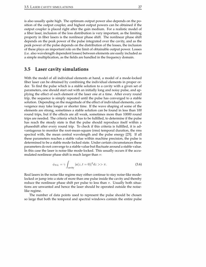
With the model of all individual elements at hand, a model of a mode-lockedfiber laser can be obtained by combining the individual elements in proper or-der. To find the pulse which is a stable solution to a cavity with a given set ofparameters, one should start out with an initially long and noisy pulse, and ap-plying the effect of each element of the laser one at a time. After every roundtrip, the sequence is simply repeated until the pulse has converged to a stablesolution. Depending on the magnitude of the effect of individual elements, con-vergence may take longer or shorter time. If the wave shaping of some of theelements are strong, sometimes a stable solution can be found in less than 100round trips, but if the effects are all weak, sometimes more than 10000 roundtrips are needed. The criteria which has to be fulfilled, to determine if the pulsehas reach the steady state is that the pulse should reproduce itself within aphaseshift after every round trip. To check if this criteria is fulfilled, it is ad-vantageous to monitor the root-mean-square (rms) temporal duration, the rmsspectral with, the mean central wavelength and the pulse energy [25]. If allthese parameters reaches a stable value within machine precision, the pulse isdetermined to be a stable mode-locked state. Under certain circumstances theseparameters do not converge to a stable value but fluctuate around a stable value.In this case the laser is noise-like mode-locked. This usually occurs if the accu-mulated nonlinear phase shift is much larger than π:
φNL = γ
∫
cavity|a(z, t = 0)|2dz >> π. (3.6)
Real lasers in the noise-like regime may either continue to stay noise-like mode-locked or jump into a state of more than one pulse inside the cavity and therebyreduce the nonlinear phase shift per pulse to less than π. Usually both situa-tions are unwanted and hence the laser should be operated outside the noise-like regime.
The number of data points used to represent the pulse should be chosenso large that both the temporal and spectral windows contain the entire pulse
28 CHAPTER 3 - SIMULATION OF FIBER LASERS
(within machine precision) at every point in the cavity. 2048-8192 points areusually enough depending on the laser.
Combining the elements in sequence is straight forward, except when thecoupling between pulses propagating both directions through the gain mediumis included. However, as it is only the average power which saturates the gainmedium, the average power of the pulse on each pass through the gain mediumcan be calculated and stored numerically as a function of position in the gainfiber. The average power of the pulse propagation in the opposite direction canhence be interpolated from the stored values from the previous pass.
3.6 Numerical simulations of a 80 MHz fiber laser
With the developed model at hand, it is now in principle possible to simulate awide range of different mode-locked fiber lasers. The output from the laser de-pends on many different parameters, such as fiber characteristics, pump power,the arrangement of the comprising components and cavity length. One param-eter is however dominant in the determination of the lasing regime, and this isthe net cavity dispersion, ∆β2. In order to illustrate simulations with the numer-ical model and to illustrate the dependence of net cavity dispersion, calculationson a realistic 80 MHz fiber laser are now presented.
HRGrating SAMPM Yb Fiber
Compressor
0.25m PM splitterPM WDM980/1030
IsolatorOutput
λ/2
976nm
SM Pump976nm
0.36m PM fiber 0.36m PM fiber
λ/4
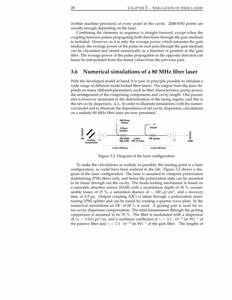
Figure 3.2: Diagram of the laser configuration.
To make the calculations as realistic as possible, the starting point is a laserconfiguration, as could have been realized in the lab. Figure 3.2 shows a dia-gram of the laser configuration. The laser is assumed to comprise polarizationmaintaining (PM) fibers only, and hence the polarization state can be assumedto be linear through out the cavity. The mode-locking mechanism is based ona saturable absorber mirror (SAM) with a modulation depth of 30 %, nonsat-urable losses of 15 %, a saturation fluence of ∼ 100 µJ/cm2, and a recoverytime of 0.5 ps. Output coupling (OC) is taken through a polarization main-taining (PM) splitter and can be tuned by rotating a quarter wave plate. In thenumerical simulations an OC of 60 % is used. A grating pair is used for in-tra cavity dispersion compensation. The total transmission through the gratingcompressor is assumed to be 70 %. The fiber is modulated with a dispersionof β2 = 0.024 ps2/m, and a nonlinear coefficient of γ = 3.5 · 10−3 (m W)−1 ofthe passive fiber and γ = 7.4 · 10−3 (m W)−1 of the gain fiber. The lengths of
3.6. NUMERICAL SIMULATIONS OF A 80 MHZ FIBER LASER 29
0
10
20
30
40
50
60
0 200 400 600 800 1000
∆trm
s / p
s
Round trips
φNL = πφNL = 2π
0
0.5
1
-100 0 100
Pow
er /
a.u.
Time / ps
0
1
2
3
4
5
6
7
0 200 400 600 800 1000
∆λrm
s / n
m
Round trips
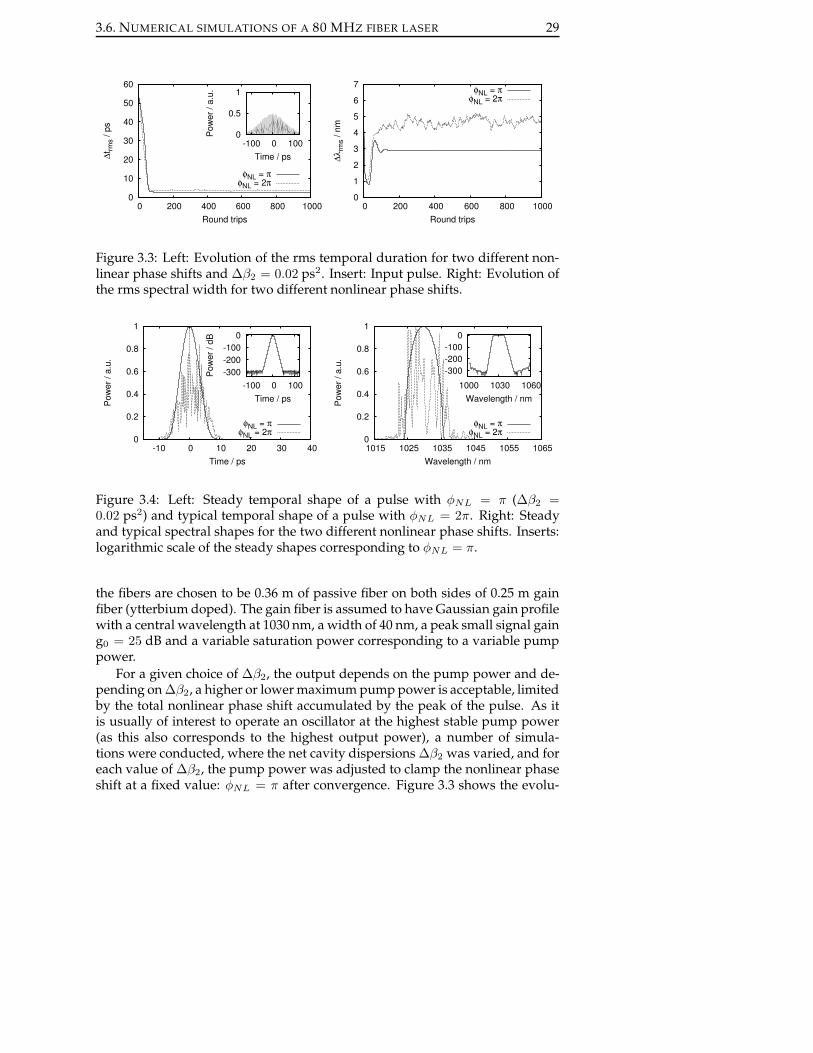
φNL = πφNL = 2π
Figure 3.3: Left: Evolution of the rms temporal duration for two different non-linear phase shifts and ∆β2 = 0.02 ps2. Insert: Input pulse. Right: Evolution ofthe rms spectral width for two different nonlinear phase shifts.
0
0.2
0.4
0.6
0.8
1
-10 0 10 20 30 40
Pow
er /
a.u.
Time / ps
φNL = πφNL = 2π
-300-200-100
0
-100 0 100
Pow
er /
dB
Time / ps
0
0.2
0.4
0.6
0.8
1
1015 1025 1035 1045 1055 1065
Pow
er /
a.u.
Wavelength / nm
φNL = πφNL = 2π
-300-200-100
0
1000 1030 1060Wavelength / nm
Figure 3.4: Left: Steady temporal shape of a pulse with φNL = π (∆β2 =0.02 ps2) and typical temporal shape of a pulse with φNL = 2π. Right: Steadyand typical spectral shapes for the two different nonlinear phase shifts. Inserts:logarithmic scale of the steady shapes corresponding to φNL = π.
the fibers are chosen to be 0.36 m of passive fiber on both sides of 0.25 m gainfiber (ytterbium doped). The gain fiber is assumed to have Gaussian gain profilewith a central wavelength at 1030 nm, a width of 40 nm, a peak small signal gaing0 = 25 dB and a variable saturation power corresponding to a variable pumppower.
For a given choice of ∆β2, the output depends on the pump power and de-pending on ∆β2, a higher or lower maximum pump power is acceptable, limitedby the total nonlinear phase shift accumulated by the peak of the pulse. As itis usually of interest to operate an oscillator at the highest stable pump power(as this also corresponds to the highest output power), a number of simula-tions were conducted, where the net cavity dispersions ∆β2 was varied, and foreach value of ∆β2, the pump power was adjusted to clamp the nonlinear phaseshift at a fixed value: φNL = π after convergence. Figure 3.3 shows the evolu-

30 CHAPTER 3 - SIMULATION OF FIBER LASERS
5
10
15
20
25
30
35
0 5 10 15 20 25 30 35 40 45 50
Spe
ctra
l wid
th (F
WH
M) /
nm
∆β2 /10-3ps2
0
20
40
60
80
100
120
0 5 10 15 20 25 30 35 40 45 50
Out
put p
ower
/ m
W
∆β2 /10-3ps2
Figure 3.5: Left: Maximum spectral width vs. net cavity dispersion, ∆β2, at apump power corresponding to a nonlinear phase shift, φNL = π. Right: Maxi-mum output power.
0 2 4 6 8
10 12 14 16 18
0 5 10 15 20 25 30 35 40 45 50Out
put p
ulse
dur
atio
n (F
WH
M) /
ps
∆β2 / 10-3ps2
0.05
0.1
0.15
0.2
0.25
0.3
0.35
0.4
0 5 10 15 20 25 30 35 40 45 50Tran
sfor
m li
mite
d pu
lse
dura
tion
(FW
HM
) / p
s
∆β2 /10-3ps2
Figure 3.6: Left: Chirped output pulse duration width vs. net cavity dispersion,∆β2, at a pump power corresponding to a nonlinear phase shift, φNL = π. Right:Transform limited pulse duration after external pulse compression calculatedfrom the spectral width.
tion of the rms temporal duration and spectral width for the particular case of∆β2 = 0.02 ps2, and figure 3.4 shows the steady temporal and spectral shape ofthe pulse on both a linear and logarithmic scale. In the insert of figure 3.4 (left)the input pulse can also bee seen.
For a total nonlinear phase shift much larger than ∼ π, the calculations donot converge to a stable pulse, but to the a noise-like pulse which fluctuates fromround trip to round trip. In figure 3.3 the evolution of the rms temporal durationand spectral width can also be seen for the case where the pump power has beenincreased to give a nonlinear phase shift of φNL ∼ 2π (dotted line). Figure 3.4also shows a typical output pulses after convergence to the noise like state.
By varying ∆β2 while maintaining φNL = π, trends of the maximum out-put power, the spectral width, the temporal duration, and the transform limitedpulse duration calculated from the spectral width were calculated vs. ∆β2. The

3.6. NUMERICAL SIMULATIONS OF A 80 MHZ FIBER LASER 31
results of the simulations can be seen in figures 3.5-3.6 The trends are clear: atsmall values of ∆β2, broader spectra, externally compressible to shorter pulsesare possible. Also if external compression is not wanted, shortest output pulsedurations is obtained for small values of ∆β2. However at smaller values of∆β2, the maximum output power is also smaller. It is, however, interesting tonotice, that at a net cavity dispersion of ∆β2 = 0.047 ps2, the dispersion of thegrating compressor is zero, and hence stable mode-locked lasing is obtainedwithout intra cavity dispersion compensation. This property is further investi-gated in chapter 8.
Calculations have only been carried out for positive values of net cavity dis-persion, as the laser enters the soliton regime for negative values of ∆β2. In thesoliton regime stable lasing is usually only obtained for much smaller valuesof nonlinear phase shift (i.e. ∼ 0.1 π) and as the pulse is further almost trans-form limited inside the laser in the soliton regime, the peak power is also muchhigher. Therefore high values of φNL are reached at lower output powers.
As with all numerical models, it is important not to forget the real focus:obtaining and understanding experimental results, in order to contribute to thedevelopment of physical realizable systems. Therefore the data presented inthis section should only be taken as guidelines and illustrations of what mightbe obtained experimentally. From simulations of the lasers presented in the restof this thesis it is evident, that the model is quite accurate, and good agreementsbetween simulations and experimental results have been obtained.


33
CHAPTER 4
Characterization techniques
This chapter describes some of the different developed setups for charcteriza-tion of mode-locked fiber lasers and fiber components. A setup was developedto measure chromatic dispersion of optical fibers. The setup was used to mea-sure dispersion of the fibers used in all other parts of this work. The setup waspayed by and developed on request from NKT-Research and is now used atNKT-Research to measure the dispersion of fibers in their products. The workwas done in collaboration with Thomas Vestergaard Andersen. The developedsetup for autocorrelation measurements is also introduced, and the theory be-hind autocorrelation measurements briefly discussed. Finally the concept ofpolarization maintaining fibers is introduced and a short introduction is givento the measurement of group birefringence in optical fibers.
34 CHAPTER 4 - CHARACTERIZATION TECHNIQUES
MEASUREMENT OF FIBER DISPERSION
4.1 Introduction
In the design of mode-locked fiber lasers, knowledge about the dispersion of afiber is often of key importance. The dispersion influences on the pulse prop-agation in the fiber. In a cavity it is the net dispersion (the sum of the totaldispersion of different sections calculated with sign) which has the strongest in-fluence on the laser output. Although indirect methods exist to estimate the netcavity dispersion, by e.g. looking at the sidebands in the soliton regime [70],or by changing the net dispersion while monitoring the laser output, the bestmethod is to measure the dispersion of each fiber sections separately. In otherareas of fiber optics the fiber dispersion is also of key importance. For instance,supercontinuum generation in a nonlinear fiber depends critically on the posi-tion of the zero dispersion wavelength (ZDW) and on higher order dispersionterms and knowledge about higher order terms is also of key importance whenusing a fiber for e.g. four-wave mixing [II] or supercontinuum generation. Asshown in chapter 5 knowledge of higher order dispersion terms is also relevantin fiber laser design.
The dispersion of an optical fiber can be measured in several ways. Thecommercial available systems for the telecommunication industry use the dif-ferential phase shift method, where light from a broadband light source is in-tensity modulated at high frequencies and sent through the fiber [71]. At theend of the fiber, different wavelengths have different phase shifts. The mea-surement of these different phase delays in the frequency domain relates to adelay in the time domain and, therefore, to the fiber dispersion. Commercialsystems are rather expensive and usually limited to telecommunication wave-length range (1530-1625 nm), but exist with the possibility of extended wave-length range (1200-1700 nm). Furthermore, commercial systems require ratherlong fiber lengths (i.e. >>10 m). Therefore, it is of interest to look into otherless expensive methods, which can be realized in the lab. The femtosecondtime-delay technique [72] and the white light interferometry technique [73] arethe most used techniques. The femtosecond time-delay technique is based ontime of flight experiments but requires a tunable femtosecond laser. The whitelight interferometry technique is based on a rather simple setup, where the in-terference signal from a white light source in a Michelson interferometer (withthe fiber under test in one arm) can be used to extrapolate the dispersion. Inreference [73] the temporal interference signal is measured while scanning thelength of the reference arm. A setup based on this technique has previouslybeen developed in our group and is now used at Crystal Fibre to characterizetheir fibers. The setup only requires measurement of the interference signal witha simple photo diode, but requires very accurate temporal resolution (calibratedby a He-Ne laser in the interferometer) and very high stability over the ratherlong recording time. As an alternative solution the interference signal can be

4.2. EXPERIMENTAL SETUP 35
measured spectrally with the reference arm fixed [74]. This method requires aoptical spectrum analyzer with a high resolution, but reduces the recording timeconsiderably, and hence also the requirement of high stability.
As an optical spectrum analyzer was available to us, the white light interfe-rometry method with signal measurement in the spectral domain was the obvi-ous choice. Furthermore, as the requirements on high stability were somewhatrelaxed, it was possible for us to implement the interferometer with fiber pig-tailed components. A solution which highly simplifies the use of the setup andthe inclusion of the optical spectrum analyzer.
The spectral range of the setup is limited by the the light source. Initially thesetup was only intended to be used to characterize fibers close to the emissionspectrum of ytterbium, and hence a simple ytterbium ASE (Amplified Sponta-neous Emission) source could be used as the light source. Later the setup wasmodified to use a fiber-pigtailed super continuum source now commerciallyavailable from Koheras [75]. This increased the spectral range to∼ 550-1800 nm.
4.2 Experimental setup
Figure 4.1 shows a diagram of the experimental setup. The ASE source wasbased on a short piece of ytterbium doped fiber pumped through a WDM witha 150 mW 980 nm diode laser. Lasing was prevented by sending the outputthrough two fiber pigtailed isolators spliced to the interferometer.
Translation stageFiber collimator
50/50
Polarizer
To spectrum analyzer
(yb ASE source)Whiht light source
Test fiber
Butt couplingLens Lens
Figure 4.1: Diagram of the experimental setup of the white light interferometer.
The Michaelson-like interferometer was based on a 50:50 fused fiber cou-pler working as the beam splitter. In one arm the fiber under test could beinserted either by butt-coupling the fiber or by using a lens system to maxi-

36 CHAPTER 4 - CHARACTERIZATION TECHNIQUES
mize the coupling between the standard fiber and the fiber under test. Thislens setup was primarily used when measuring the dispersion of hollow corephotonic bandgap (HC-PBG) fibers as a butt-coupling to such a fiber causes aFresnel back-reflection at the interface due to different refractive indexes of thecores. The other end of the test fiber was butt coupled to a mirror. In the ref-erence arm, the beam was collimated and reflected on a mirror positioned on atranslation stage.
All the fibers in the setup were non-polarization maintaining (non-PM), butby avoiding bending the fibers strongly, a large change in polarization state be-tween the two arms could be avoided. A small difference in polarization stateonly results in smaller fringes and is acceptable. If the fiber under test waspolarization maintaining (PM) a bulk polarizer could be inserted in the refer-ence arm to pick out the polarization state interfering with light from one of thepolarization axis of the test fiber. The rotation angle of the polarizer was foundby minimizing the beats in the spectral interference pattern.
The choice of a fiber based interferometer resulted in an increased sensi-tive to environmental perturbations and especially air convection influencedthe measurement. The environmental perturbations resulted in a drifting fringepattern, due to a changing phase difference between the two arms. To minimizethis effect, the setup was placed in an air tight box. Due to the fast recordingtime of the optical spectrum analyzer, a sufficiently slow drift time was easilyreached.
If the fibers in the two arms of the interferometer are of different length, itwill result in a contribution to the measured dispersion. In addition the couplerand the lens coupling setup will also contribute to the measured dispersion.However, as dispersion of different elements adds linearly, the dispersion of thesetup can be measured separately and subtracted and hence the balancing of thedispersion of the two arms is not critical.
As the light source is broadband and incoherent, the optical path length ofthe two arms must be matched. This is achieved by scanning the stage. Tempo-rally an interference signal can be observed by scanning the stage, and figure 4.2shows such a signal. The midpoint is referred to as ”T=0”. When the stage isclose to ”T=0” interference fringes can be observed in the spectrum.
4.3 Theory
If E1 and E2 are the time independent complex electric field amplitudes at thedetector of the reference arm and test fiber arm respectively, and if φ1(ω) andφ2(ω) are the accumulated phases in the two arms, then the intensity is given by
I(ω) = |E1|2 + |E2|2 + 2E1E2 cos(φ2(ω)− φ1(ω)).
The frequency dependent phase difference contains a contribution from the setup,a contribution from the test fiber and a contribution from the free space section

4.3. THEORY 37
1.8 2
2.2 2.4 2.6 2.8
3 3.2 3.4 3.6 3.8
4
-0.8 -0.6 -0.4 -0.2 0 0.2 0.4 0.6 0.8
Pow
er /
a.u.
Time / ps
Figure 4.2: Temporal signal from the white light setup around the ”T=0” point.
in the reference arm:
∆φ(ω) ≡ φ2(ω)− φ1(ω) = ∆φs(ω) + φf (ω)− ω
cd, (4.1)
where d is the distance between the ”T=0” point of the setup without test fiberand the ”T=0” point with the fiber. ∆φ(ω) can be measured modulus 2π by mea-suring the spectral position of the fringes. The distance between two successivefringes corresponds to an increase or decrease in ∆φ(ω) of 2π. If the secondderivative of the phase difference with respect to frequency is calculated, thecontribution from the stage position disappears:
∂2
∂ω2∆φ(ω) =
∂2
∂ω2∆φs(ω) +
∂2
∂ω2φf (ω).
∂2
∂ω2 ∆φs(ω) can be calculated from a separate but similar measurement withouttest fiber and subtracted from ∂2
∂ω2 ∆φ(ω). The last term relates directly to thedispersion of the fiber:
∂2
∂ω2φf (ω) = 2β2(ω)L,
where L is the length of test fiber, and β2 is the group velocity dispersion. Onceβ2(ω) is known, the usual dispersion parameter is easily calculated from theequation:
D = −2πc
λ2β2.
Higher order dispersion terms are contained in β2(ω) and are found by expand-ing β2(ω) around a center frequency ω0:
β2(ω) = β2(ω0) + β3(ω0)(ω − ω0) +1
2β4(ω0)(ω − ω0)
2 + ... (4.2)

38 CHAPTER 4 - CHARACTERIZATION TECHNIQUES
The propagation constant, β(ω)′, which was introduced in equation 2.19 as aparameter in the nonlinear Schrodinger equation, and is relevant for laser cavitycalculations, can now be found by integrating equation 4.2 twice:
β(ω)′ =1
2β2(ω0)(ω − ω0)
2 +1
6β3(ω0)(ω − ω0)
3 +1
24β4(ω0)(ω − ω0)
4 + ... (4.3)
where the integration constants have been set to zero, as they only correspondto a change of linear phase and a translation of the pulse on the time axis andhence are not relevant for the slowly varying envelope.
4.4 Dispersion measurements
To illustrate how the calculations are made, an example based on a hollow corephotonic bandgap fiber (HC-PBG) fiber from Crystal Fibre is presented below.Figure 4.3 (left) shows a cross section of the fiber, and figure 4.3 (right) the trans-mission spectrum.
-25
-20
-15
-10
-5
0
900 1000 1100 1200Tr
ansm
issi
on /
dB
Wavelength / nm
Figure 4.3: Left: SEM image of the cross section of the HC-PBG fiber. Right:Transmission spectrum through 2 m of the HC-PBG fiber.
The fiber is interesting because it has negligible nonlinearity and a highanomalous dispersion at 1030 nm and as shown in chapter 5 it can be used forpulse compression after external amplifications of a fiber laser without degrad-ing pulse quality. Figure 4.4 shows a typical spectrum with interference fringes.
The phase difference can be constructed by noting that the phase must haveincreased or decreased with 2π at the peak of each fringe. As the ∆φ(ω) con-tains a quadratic term (the GVD), it will as a function of frequency have a localextremum point. By changing the linear term in eq. 4.1 (e.g. by moving thestage), the position of the extremum point can be moved. This turning pointcan be seen in figure 4.4 close to 1040 nm. The position of the turning pointdoes not influence on the dispersion, but is usually best placed in the middleof the spectrum in order to get maximum resolution on the fringes. The sign

4.4. DISPERSION MEASUREMENTS 39
-75-70-65-60-55-50-45-40-35-30-25
980 1000 1020 1040 1060 1080 1100 1120
Pow
er /
dB
Wavelength / nm
-60
-55
-50
-45
-40
-35
-30
-25
1020 1030 1040 1050 1060 1070
Pow
er /
dB
Wavelength / nm
∆φ(λi)∆φ(λi+1) = ∆φ(λi) + 2π∆φ(λi+2) = ∆φ(λi) + 4π
Figure 4.4: Left: Measured spectrum with interference fringes. The position ofthe turning point is found around 1040 nm where the slow modulation revealsthat the linear term in the phase difference is zero. Right: Zoom on the regionaround 1045 nm. The phase difference can be constructed by adding 2π at eachlocal maximum.
-400
-200
0
200
400
600
800
980 1000 1020 1040 1060 1080 1100 1120
Pha
se /
rad
Wavelength / nm
-400
-200
0
200
400
600
800
1.7 1.75 1.8 1.85 1.9 1.95
Pha
se /
rad
Frequency / 1015 rad/s
6th-12th order fit
Figure 4.5: Left: Phase versus wavelength. Right: Phase versus frequency. Sixpolynomial fits of order 6 to 12 are shown, and all fit the the measured pointswell.
of the quadratic term in ∆φ(ω) can be found by noting that if the length of thestage arm is increased (linear term in eq. 4.1 decreased), the turning point willmove towards longer wavelengths (lower frequencies) if the GVD is negativeand towards shorter wavelengths if the GVD is positive. The resulting phasedifference can be seen in figure 4.5.
The second derivative of the phase difference is found by fitting a polyno-mial to ∆φ(ω) and deriving it twice. The order of the polynomial must of coursebe chosen large enough, that the polynomial coincides with the measured pointsover the entire frequency range. Figure 4.5 (right) shows polynomial fits of order6 to 12 to ∆φ(ω). For this particular measurement, polynomials of order higherthan 5 gives accurate fits within the measured range. The resulting dispersionsoriginating from the 6 different polynomials can seen in figure 4.6 (left). As

40 CHAPTER 4 - CHARACTERIZATION TECHNIQUES
0
50
100
150
200
250
980 1000 1020 1040 1060 1080 1100 1120
D /
ps/(n
m k
m)
Wavelength / nm
6th-12th order fit
0
50
100
150
200
250
980 1000 1020 1040 1060 1080 1100 1120
D /
ps/(n
m k
m)
Wavelength / nm
Axis 1Axis 2
Figure 4.6: Left: The calculated dispersion of the HC-PBG fiber for the 6 differentpolynomials. The curves almost coincide in the middle of the interval while theydiffer significantly at the edges. Right: Dispersions of the two polarization axesof the fiber.
can be seen, the calculated dispersion depends on the order of the polynomial.However in the middle ∼ 80 % of the measured interval, the curves coincideswithin an acceptable uncertainty. Only at the edges, the dispersion is inaccu-rately determined. However, as it is unlikely that the slope of the dispersionchanges drastically near the edges of the measured interval, one can chose thepolynomial of lowest order, which also fits the data. In this case: order 6. Theaccuracy of the setup was tested by measuring the dispersion of well-knownfibers such as SMF28 [76] and HI1060 Flexcore [77], and in both cases excellentagreement with known values were found.
The HC-PBG fiber was observed to be birefringent and the dispersion ofboth polarization axes were measured. Figure 4.6 (right) shows the measureddispersions of the two axes. The dispersion was found to be indistinguishable.
Even though the setup based on the ytterbium ASE source is well suitedfor measurements of the dispersion of components for ytterbium based fiberlasers in the relevant wavelength range, other applications require dispersionmeasurements over a broader range. For this purpose the ASE source was re-placed with a super continuum white light source [75]. The super continuum iscreated in a nonlinear photonic crystal fiber (PCF) pumped at 1060 nm with aQ-switched laser. The nonlinear fiber could be spliced directly to the setup withlow loss. In order to compensate for the limited bandwidth of the 2x2 50:50coupler it was replaced by two 1x2 50:50 thin film couplers and the Michaelson-like interferometer was changed into a Marc-Zender interferometer. With thisapproach more power was lost but by combining the two 1x2 couplers so thatidentical arms of the couplers were put in opposite arms of the interferometer,a coupling ration far from the perfect 50:50 became acceptable and the setupcould be used over the entire wavelength range of the super continuum source.
To illustrate the broad measurement range of the setup, the dispersion mea-sured from 900-1300 nm of a nonlinear PCF and the dispersion measured from

4.4. DISPERSION MEASUREMENTS 41
-40-30-20-10
0 10 20 30 40 50 60
900 1000 1100 1200 1300 1400 1500 1600 1700
D /
ps/(n
m k
m)
Wavelength / nm
White light fiberHI1060
Figure 4.7: Measured dispersion of a nonlinear PCF with a ZDW at 975 nm andof a HI1060 Flexcore fiber.
1000-1700 nm of a HI1060 Flexcore fiber can be seen in figure 4.7. The standardfiber, HI1060, exhibits a high normal dispersion (i.e. D < 0) around 1 µm, andthe nonlinear PCF has a blue shifted ZDW at 975 nm and hence exhibits anoma-lous dispersion around 1 µm. The setup has further been used to measure thedispersion of the solid core photonic bandgap fibers used in chapter 5.

42 CHAPTER 4 - CHARACTERIZATION TECHNIQUES
AUTOCORRELATION MEASUREMENTS
4.5 Introduction
Experimentally, it is often important to be able to determine the duration of apulse. The fundamental limit in pulse duration is set by the spectral width (andshape) of the pulse. This limit is know as the Fourier limit or transform limit,as it can be found by Fourier transforming the spectrum with zero phase. How-ever, a pulse may have a nonlinear chirp which cannot be removed with simpledispersive elements such as prism or grating pairs. This results in a longer min-imum pulse duration. As pulses from mode-locked lasers are often so short (i.e.<< 30 ps), that even the fastest photo diodes cannot resolve the temporal shapeof the pulse, an alternative approach has to be taken. The temporal duration of apulse can be extrapolated by measuring the interference signal of the pulse withanother short pulse as function of delay between the two pulses. Most conve-niently, a pulse can be interfered with itself. The setup for this measurement isknown as an autocorrelator, and the output as an autocorrelation trace.
4.6 Setup and theory
1
2
Figure 4.8: Diagram of the autocorrelator. The delay can be changed by scanningstage 1. By moving stage 2, the autocorrelator can be changed from interfero-metric to background free.
An autocorrelator is based on a Michaelson interferometer, which splits thepulse into two pulses: one in each arm. The two pulses are recombined withan added temporal delay. Figure 4.8 shows a diagram of the Michaelson inter-ferometer which was build to make autocorrelation measurements. One armof the autocorrelator could be scanned up to 350 ps, and was controlled by acomputer. This enables both high resolution autocorrelation measurements andlong range autocorrelation traces. With this autocorrelator, both interferometric

4.6. SETUP AND THEORY 43
autocorrelation traces (overlapped beams) and background free autocorrelationtraces (parallel but not overlapped beams) could be measured. To get an secondorder autocorrelation trace, the intensity must be squared. The easiest way tomeasure the interferometric autocorrelation trace is to use two-photon absorp-tion on the surface of a photo diode which cannot see photons at the laser wave-length, λ0, but only with wavelength λ0/2. In the range 680-1360 nm, a GaAsPphoto diode is appropriate [78], and such a photo diode (Hamamatsu G1117)was used for the interferometric autocorrelation traces. For a background freeautocorrelation trace, the beams must be crossed by focusing the two parallelbeams with the same lens into a nonlinear crystal (e.g. a BBO crystal). On theoutput side three beams emerge. The middle one is the background free auto-correlation trace. The advantage of the background free autocorrelator is that itis easier to extract the pulse duration directly from the trace. The disadvantageon a daily basis is that it is more difficult to check if the autocorrelator is prop-erly aligned. If the autocorrelator is not aligned correctly and one beam driftsas the delay is scanned, the background free autocorrelation trace can indicate apulse duration which is shorter than the actual pulse duration.
The second order interferometric autocorrelation function is calculated as:
G2(τ) =
∫ ∞
−∞
|(E(t) + E(t− τ))2|2dt, (4.4)
where τ is the variable delay between the pulses, and E(t) = A(t) exp(−iω0t).For the case of a chirped Gaussian pulse (see equation 2.35) the autocorrelationtrace can be calculated analytically:
G2(τ) ∝ 1 + 2 exp(
− 2 ln(2)
1 + C2
( τ
t0
)2)
+ 4 exp(
− 2 ln(2)
1 + C2
3 + C2
4
( τ
t0
)2)
cos( ln(2)C
1 + C2
( τ
t0
)2)
cos(ω0τ)
+ exp(
− 2 ln(2)( τ
t0
)2)
cos(2ω0τ). (4.5)
An important ratio when aligning an interferometric autocorrelator is the ratiobetween the top of the autocorrelation trace and constant background:
G2(0) : G2(∞) = 1 : 8. (4.6)
Only if this ratio is fulfilled are the measured pulse durations trustworthy. No-tice that G2(τ) consists of four terms: a constant term, a Gaussian term with nooscillations, a Gaussian term oscillating with ω0 and finally another Gaussianterm oscillating with 2ω0. In the limit of C = 0, all three Gaussian terms havesimilar widths, but in the limit where C is large, the width of the first Gaus-sian term exceeds the widths of the other terms. The top and bottom envelopesof the autocorrelation function are easily found by replacing cos(ω0τ) → 1,cos(2ω0τ)→ 1 (top envelope) and cos(ω0τ) → −1, cos(2ω0τ)→ 1 (bottom enve-lope) respectively in equation 4.5.
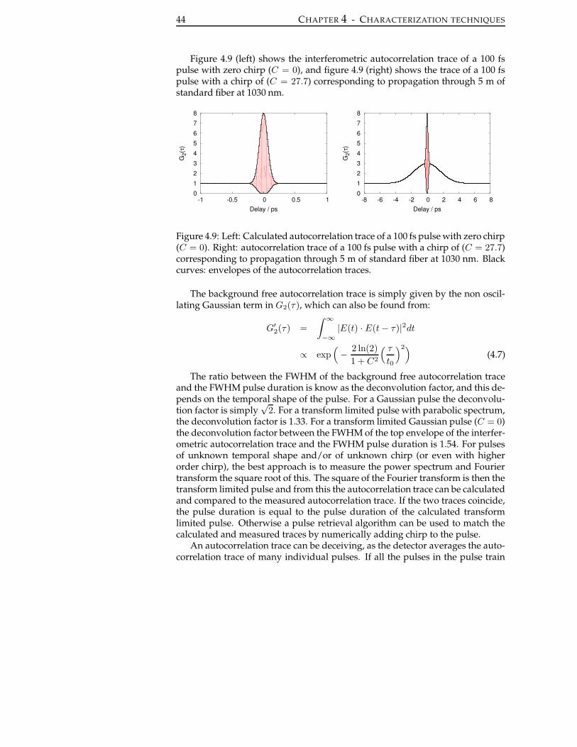
44 CHAPTER 4 - CHARACTERIZATION TECHNIQUES
Figure 4.9 (left) shows the interferometric autocorrelation trace of a 100 fspulse with zero chirp (C = 0), and figure 4.9 (right) shows the trace of a 100 fspulse with a chirp of (C = 27.7) corresponding to propagation through 5 m ofstandard fiber at 1030 nm.
0
1
2
3
4
5
6
7
8
-1 -0.5 0 0.5 1
G2(
τ)
Delay / ps
0
1
2
3
4
5
6
7
8
-8 -6 -4 -2 0 2 4 6 8
G2(
τ)
Delay / ps
Figure 4.9: Left: Calculated autocorrelation trace of a 100 fs pulse with zero chirp(C = 0). Right: autocorrelation trace of a 100 fs pulse with a chirp of (C = 27.7)corresponding to propagation through 5 m of standard fiber at 1030 nm. Blackcurves: envelopes of the autocorrelation traces.
The background free autocorrelation trace is simply given by the non oscil-lating Gaussian term in G2(τ), which can also be found from:
G′2(τ) =
∫ ∞
−∞
|E(t) · E(t− τ)|2dt
∝ exp(
− 2 ln(2)
1 + C2
( τ
t0
)2)
(4.7)
The ratio between the FWHM of the background free autocorrelation traceand the FWHM pulse duration is know as the deconvolution factor, and this de-pends on the temporal shape of the pulse. For a Gaussian pulse the deconvolu-tion factor is simply
√2. For a transform limited pulse with parabolic spectrum,
the deconvolution factor is 1.33. For a transform limited Gaussian pulse (C = 0)the deconvolution factor between the FWHM of the top envelope of the interfer-ometric autocorrelation trace and the FWHM pulse duration is 1.54. For pulsesof unknown temporal shape and/or of unknown chirp (or even with higherorder chirp), the best approach is to measure the power spectrum and Fouriertransform the square root of this. The square of the Fourier transform is then thetransform limited pulse and from this the autocorrelation trace can be calculatedand compared to the measured autocorrelation trace. If the two traces coincide,the pulse duration is equal to the pulse duration of the calculated transformlimited pulse. Otherwise a pulse retrieval algorithm can be used to match thecalculated and measured traces by numerically adding chirp to the pulse.
An autocorrelation trace can be deceiving, as the detector averages the auto-correlation trace of many individual pulses. If all the pulses in the pulse train

4.6. SETUP AND THEORY 45
are identical, there is no problem, as the average trace is then identical to the in-dividual trace. However, if there are large fluctuations from pulse to pulse, theaverage trace may resemble that of figure 4.9 (right), but instead of indicatinga chirped pulse which can be compressed by applying an appropriate amountof dispersion, the pulses could also be incompressible, as the phases of the indi-vidual pulses may be different and even very noisy. In fact figure 4.10 shows thenumerically calculated autocorrelation trace averaged over 1000 round trips ofthe noise-like mode-locked state from the example at the end of chapter 3. Thistrace is indistinguishable from a trace of a noise-free but chirped mode-lockedoutput.
0
1
2
3
4
5
6
7
8
-25 -20 -15 -10 -5 0 5 10 15 20 25
G2(
τ)
Delay / ps
Figure 4.10: Autocorrelation trace of a noise-like mode-locked output.
To distinguish between noise-free chirped pulses and of noise-like pulses,other factors have to be taken into account. For example the spectral shape canbe compared to calculated spectral shapes which differs if the pulses are noise-like. In the normal dispersion regime, the spectra tends to have very steep edgesif the laser is noise-free, whereas noise-like mode-locking leads to Gaussian-like spectra. Alternatively the amplitude noise can be measured with an RF-spectrum analyzer. The ultimate test is however, if the pulses are externallycompressible with e.g. a grating compressor.

46 CHAPTER 4 - CHARACTERIZATION TECHNIQUES
MEASUREMENT OF GROUP BIREFRINGENCE
4.7 Polarization maintaining fibers
In a fiber with perfect hexagonal symmetry (or any higher than twofold rota-tional symmetry) two orthogonal polarized modes will be degenerate [79]. Onthe other hand, if the fiber is constructed to be asymmetric, so that it only hastwofold rotational symmetry the propagation constants of two orthogonal po-larized (i.e. linear polarized) modes, βx and βy, will in general be different, andthe fiber is said to be birefringent. Birefringence is typically obtained througheither form birefringence (asymmetric core shapes) or stress induced birefrin-gence (by embedding stress rods in the material with different thermal expan-sion coefficients and hence incorporating a strain in the material).
If the propagation constants are expanded around a frequency, ω0:
β(ω) = n(ω)ω
c= β0 + β1(ω − ω0) + β2(ω − ω0)
2 + ..., (4.8)
where:
βk =(∂kβ
∂ωk
)
, (4.9)
then β0 and β1 are related to the phase and group velocity respectively:
β0 =ω0
vp= n(ω0)
ω0
c(4.10)
β1 =1
vg=
ng
c=
1
c
(
n(ω0) + ω0∂n
∂ω(ω0)
)
(4.11)
where vp is the phase velocity, vg the group velocity, and ng the group index.Physically speaking, the envelope of an optical pulse moves at the group veloc-ity, while the phase underneath the envelope moves at the phase velocity. Ina birefringent fiber both the β0 and β1 term will in general differ for the twodifferent polarization directions. As shown in section 4.4, the group velocitydispersion, β2, and higher order terms can often be assumed to be identical forthe two orthogonal polarization directions.
The group birefringence, ∆ng , is defined as: ∆ng = |ng,x − ng,y| and knowl-edge about the group birefringence is important when working with pulse prop-agation in birefringent fibers, as it determines the walk-off between pulses launc-hed in the different axis of the fiber.
In general the birefringence of a fiber is also an important property whendesigning mode-locked fiber lasers. If a fiber is birefringent, then light polar-ized only along one axis of the fiber is prohibited from coupling into the otherpolarization axis. This is true even if the fiber is twisted, so that the polarizationaxis turns along its length. If the twist is sufficiently slow, the light can gradu-ally rotate its polarization state together with the polarization axis of the fiber.
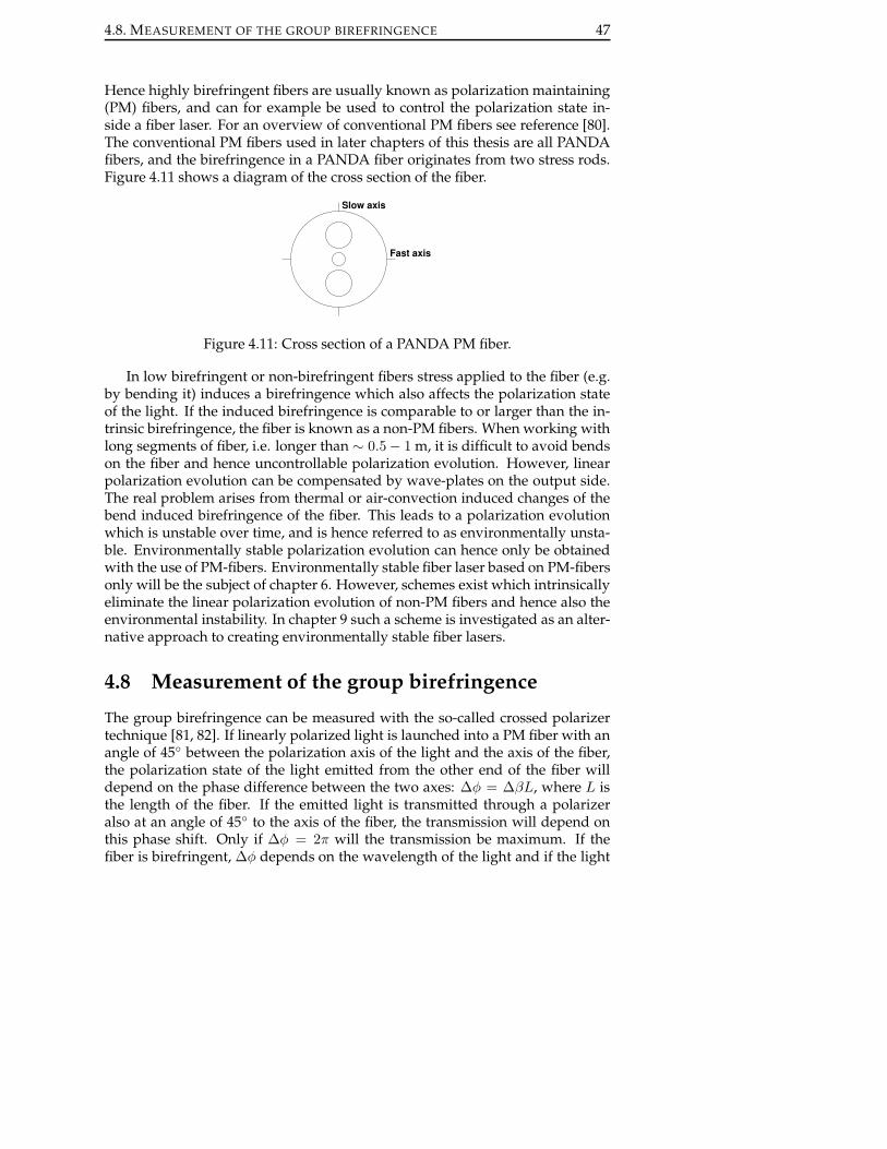
4.8. MEASUREMENT OF THE GROUP BIREFRINGENCE 47
Hence highly birefringent fibers are usually known as polarization maintaining(PM) fibers, and can for example be used to control the polarization state in-side a fiber laser. For an overview of conventional PM fibers see reference [80].The conventional PM fibers used in later chapters of this thesis are all PANDAfibers, and the birefringence in a PANDA fiber originates from two stress rods.Figure 4.11 shows a diagram of the cross section of the fiber.
Slow axis
Fast axis
Figure 4.11: Cross section of a PANDA PM fiber.
In low birefringent or non-birefringent fibers stress applied to the fiber (e.g.by bending it) induces a birefringence which also affects the polarization stateof the light. If the induced birefringence is comparable to or larger than the in-trinsic birefringence, the fiber is known as a non-PM fibers. When working withlong segments of fiber, i.e. longer than ∼ 0.5− 1 m, it is difficult to avoid bendson the fiber and hence uncontrollable polarization evolution. However, linearpolarization evolution can be compensated by wave-plates on the output side.The real problem arises from thermal or air-convection induced changes of thebend induced birefringence of the fiber. This leads to a polarization evolutionwhich is unstable over time, and is hence referred to as environmentally unsta-ble. Environmentally stable polarization evolution can hence only be obtainedwith the use of PM-fibers. Environmentally stable fiber laser based on PM-fibersonly will be the subject of chapter 6. However, schemes exist which intrinsicallyeliminate the linear polarization evolution of non-PM fibers and hence also theenvironmental instability. In chapter 9 such a scheme is investigated as an alter-native approach to creating environmentally stable fiber lasers.
4.8 Measurement of the group birefringence
The group birefringence can be measured with the so-called crossed polarizertechnique [81, 82]. If linearly polarized light is launched into a PM fiber with anangle of 45◦ between the polarization axis of the light and the axis of the fiber,the polarization state of the light emitted from the other end of the fiber willdepend on the phase difference between the two axes: ∆φ = ∆βL, where L isthe length of the fiber. If the emitted light is transmitted through a polarizeralso at an angle of 45◦ to the axis of the fiber, the transmission will depend onthis phase shift. Only if ∆φ = 2π will the transmission be maximum. If thefiber is birefringent, ∆φ depends on the wavelength of the light and if the light

48 CHAPTER 4 - CHARACTERIZATION TECHNIQUES
transmitted through the fiber is from a broadband light source, the transmittedspectrum will have spectral fringes. The group birefringence can be found fromthese spectral fringes, by noting that:
∂
∂λ∆φ = −2πc
λ2L
∂
∂ω∆β = −2π
λ2L∆ng. (4.12)
The distance between two successive fringes corresponds to an increase in∆φ of 2π, and hence:
∆ng =λ2
L∆λ, (4.13)
where ∆λ is the fringe separation.To exemplify the method, the group birefringence of the HC-PBG fiber used
in chapter 5 (shown in figure 4.3) was measured. An ytterbium ASE source wasused as light source and a fringe separation of 10.3 nm was measured at 1030 nmon a 3.34 m long piece of fiber. This corresponds to a group birefringence of3.1 ·10−5 and a group velocity mismatch of 103 fs/m. In contrast to standard PMfibers, the birefringence in this fiber is a result of a deviation from the intendedsymmetric shape.
4.9 Summary
In summary three different setups for characterization of mode-locked fiberlasers and fiber components have been presented. The setup for measurementof fiber dispersion have been applied to measure the dispersion of all the fibersused in the mode-locked lasers in this thesis. The autocorrelator was used tocharacterize the outputs from the constructed lasers, and finally the setup formeasurement of group birefringence have been used to verify the birefringenceof the HC-PBG fiber used in chapter 5 and to calculate group velocity mismatchin the PM fiber used in chapter 9 for environmentally stable nonlinear polariza-tion rotation in an all-PM mode-locked fiber laser.

49
CHAPTER 5
Solid core photonic bandgap fiberlaser
This chapter describes the results of the first mode-locked fiber laser using solid-core photonic bandgap (SC-PBG) fiber for intra cavity dispersion compensation.Limitations in terms of obtainable pulse durations have been explored, and wasfound to be limited by the high third order dispersion of the SC-PBG fiber. Af-ter external amplification and external compression in a hollow-core photonicbandgap (HC-PBG), 158 fs 5.3 nJ pulses were obtained at a central wavelengthof 1030 nm from this very compact all-fiber based system, and the result is a sig-nificant step toward a femtosecond ytterbium based fiber laser system with nosections of free space optics. The SC-PBG fiber was spliced to a standard fiber,and hence enables fiber oscillators without sections of free-space optics.

50 CHAPTER 5 - SOLID CORE PHOTONIC BANDGAP FIBER LASER
5.1 Introduction
Standard fibers have a large normal dispersion at the lasing wavelength of ytter-bium and one of the main problems using ytterbium as gain media in fiber lasersis the lack of fiber components with anomalous dispersion at this wavelength.Because of the high dispersion of standard fibers, dispersion compensating el-ements are necessary in fiber lasers to obtain broad spectra, which can resultin short femtosecond pulses. Otherwise the spectrum narrows and only longerpulses are possible.
The laser presented in chapter 6 uses a bulk transmission grating pair forintra cavity dispersion compensation. Although compact and stable, a trans-mission grating excludes the possibility of making an implementation with nofree space sections. All-fiber implementations are preferable, as it increases thestability, compactness and possibly reduces the cost.
A very elegant fiber based solution is the use of a chirped fiber Bragg Grat-ing. Dispersion compensation in fiber lasers based on chirped fiber Bragg grat-ing has been researched since the mid-nineties [83] and recently a very elegantand compact all-fiber 100 fs, 4 nJ system based on a transmitting chirped fiberBragg grating as output coupler, and an amplifier pumped with the same pumpsingle-mode fiber-pigtailed diode as the oscillator, has been demonstrated byIMRA [84].
An alternative solution to fiber based intracavity dispersion compensation isthe use of photonic bandgap fibers (PBGs). As opposed to normal fibers wherelight is bound due to a higher refractive index of the core compared to the sur-rounding cladding, bound modes in PBGs are found due to a photonic bandgapin a micro structured cladding with a higher average index than the core. Aguidance band is created in the core where light of certain wavelengths is notallowed to penetrate into the cladding [18]. This spectral guidance band of PBGsis usually quite narrow and the dispersion of PBGs is strongly affected by thehigh loss at the edges of the guidance band. The dispersion changes from highlynormal close to the short wavelength edge to highly anomalous near the longwavelength edge, with a zero dispersion wavelength in between. By scalingthe transverse dimensions of the fiber the position of the spectral transmissionband can be moved and anomalous dispersion at any wavelength is in princi-ple possible. Hollow-core photonic bandgap (HC-PBG) fibers have existed forsome years now [18] and quite recently solid-core photonic bandgap (SC-PBG)fibers have also been demonstrated [85, 86]. Using PBG fibers for dispersioncompensation has the advantage that the anomalous dispersion of the cavitycan be changed simply by changing the length of the PBG fiber. Furthermore,PBG fibers can be manufactured in lengths (i.e. > 100 m), sufficient for manymode-locked lasers and hence the use of PBG fiber potentially simplifies mass-production.
Previously mode-locked fiber lasers have been demonstrated with the use ofstandard photonic crystal fibers (PCFs) [87] and HC-PBG fibers [88]. HC-PBG
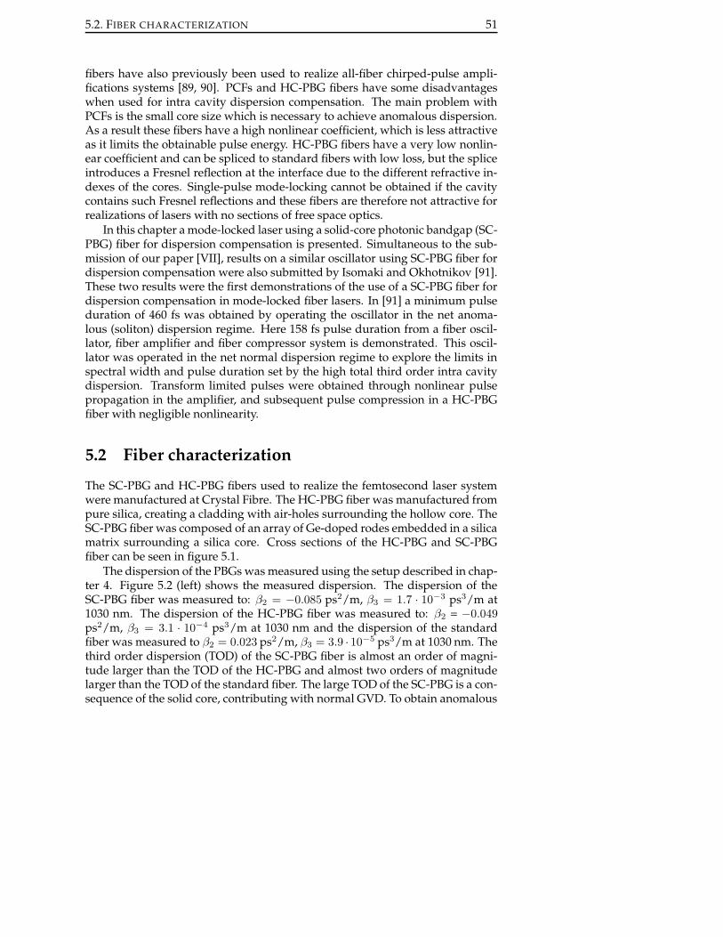
5.2. FIBER CHARACTERIZATION 51
fibers have also previously been used to realize all-fiber chirped-pulse ampli-fications systems [89, 90]. PCFs and HC-PBG fibers have some disadvantageswhen used for intra cavity dispersion compensation. The main problem withPCFs is the small core size which is necessary to achieve anomalous dispersion.As a result these fibers have a high nonlinear coefficient, which is less attractiveas it limits the obtainable pulse energy. HC-PBG fibers have a very low nonlin-ear coefficient and can be spliced to standard fibers with low loss, but the spliceintroduces a Fresnel reflection at the interface due to the different refractive in-dexes of the cores. Single-pulse mode-locking cannot be obtained if the cavitycontains such Fresnel reflections and these fibers are therefore not attractive forrealizations of lasers with no sections of free space optics.
In this chapter a mode-locked laser using a solid-core photonic bandgap (SC-PBG) fiber for dispersion compensation is presented. Simultaneous to the sub-mission of our paper [VII], results on a similar oscillator using SC-PBG fiber fordispersion compensation were also submitted by Isomaki and Okhotnikov [91].These two results were the first demonstrations of the use of a SC-PBG fiber fordispersion compensation in mode-locked fiber lasers. In [91] a minimum pulseduration of 460 fs was obtained by operating the oscillator in the net anoma-lous (soliton) dispersion regime. Here 158 fs pulse duration from a fiber oscil-lator, fiber amplifier and fiber compressor system is demonstrated. This oscil-lator was operated in the net normal dispersion regime to explore the limits inspectral width and pulse duration set by the high total third order intra cavitydispersion. Transform limited pulses were obtained through nonlinear pulsepropagation in the amplifier, and subsequent pulse compression in a HC-PBGfiber with negligible nonlinearity.
5.2 Fiber characterization
The SC-PBG and HC-PBG fibers used to realize the femtosecond laser systemwere manufactured at Crystal Fibre. The HC-PBG fiber was manufactured frompure silica, creating a cladding with air-holes surrounding the hollow core. TheSC-PBG fiber was composed of an array of Ge-doped rodes embedded in a silicamatrix surrounding a silica core. Cross sections of the HC-PBG and SC-PBGfiber can be seen in figure 5.1.
The dispersion of the PBGs was measured using the setup described in chap-ter 4. Figure 5.2 (left) shows the measured dispersion. The dispersion of theSC-PBG fiber was measured to: β2 = −0.085 ps2/m, β3 = 1.7 · 10−3 ps3/m at1030 nm. The dispersion of the HC-PBG fiber was measured to: β2 = −0.049ps2/m, β3 = 3.1 · 10−4 ps3/m at 1030 nm and the dispersion of the standardfiber was measured to β2 = 0.023 ps2/m, β3 = 3.9 · 10−5 ps3/m at 1030 nm. Thethird order dispersion (TOD) of the SC-PBG fiber is almost an order of magni-tude larger than the TOD of the HC-PBG and almost two orders of magnitudelarger than the TOD of the standard fiber. The large TOD of the SC-PBG is a con-sequence of the solid core, contributing with normal GVD. To obtain anomalous

52 CHAPTER 5 - SOLID CORE PHOTONIC BANDGAP FIBER LASER
Figure 5.1: Left: SEM image of the cross section of the HC-PBG fiber. Right:Cross section of the SC-PBG fiber.
GVD at a certain wavelength, the long wavelength edge of the transmissionband has to be moved closer as the waveguide contributes with a larger anoma-lous GVD here. The TOD, however, is also larger here and as a consequencethe resulting TOD will be higher. The mode field diameter (MFD) of the SC-PBG fiber was 8 µm and hence the fiber has a lower nonlinear coefficient com-pared to the standard fiber (MFD = 6 µm). The HC-PBG fiber was observedto be birefringent and the group birefringence of the fiber was measured to be∆ng = 3.1 · 10−5 with the setup described in chapter 4. The dispersion of bothpolarization axes was indistinguishable. The SC-PBG fiber on the other handwas not observed to be birefringent.
-0.5
-0.4
-0.3
-0.2
-0.1
0
0.1
0.2
1000 1020 1040 1060 1080 1100
β 2(λ
) / p
s2 /m
Wavelength / nm
SC-PBGHC-PBG
HI1060
-30
-25
-20
-15
-10
-5
1000 1020 1040 1060 1080 1100
Inse
rtion
loss
/ dB
Wavelength / nm
SC-PBG
Figure 5.2: Left: Dispersion of the SC-PBG, HC-PBG and standard fiber. Right:The insertion loss of the 0.36 m long SC-PBG fiber.
5.3 Laser design
Figure 5.3 shows a diagram of the laser system. The cavity of the oscillator con-sists of a WDM, 8.5 cm of highly doped ytterbium fiber (1200 dB/m absorption
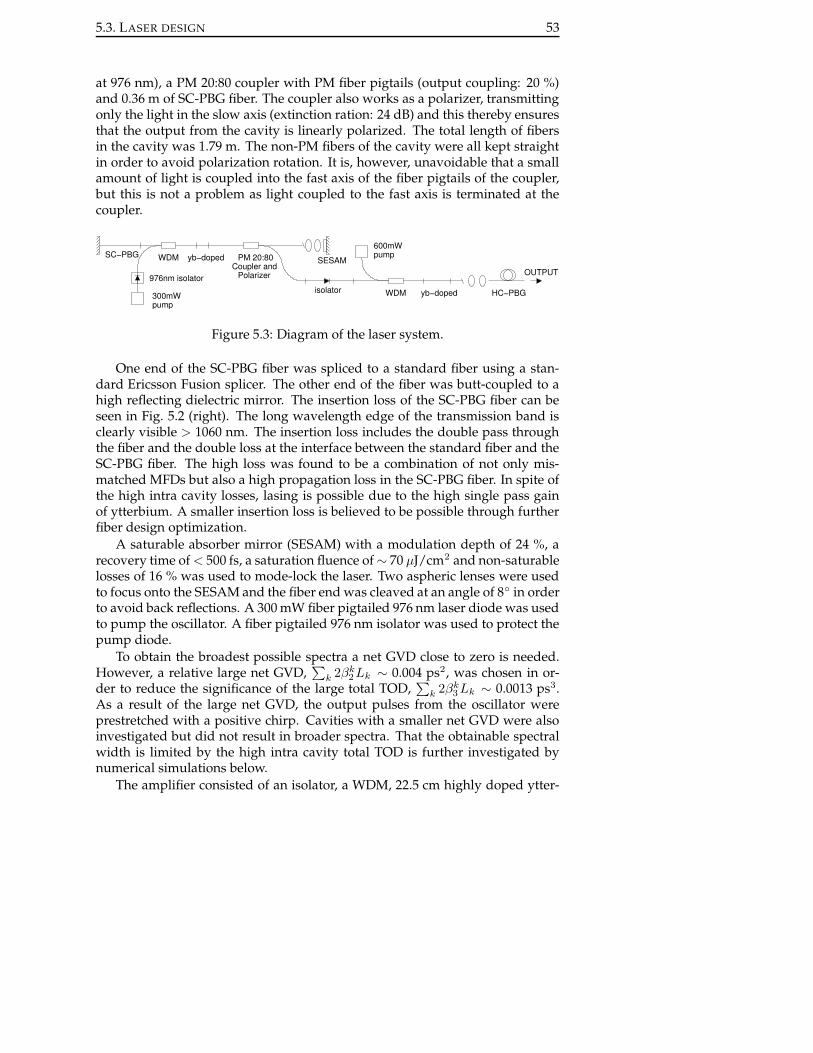
5.3. LASER DESIGN 53
at 976 nm), a PM 20:80 coupler with PM fiber pigtails (output coupling: 20 %)and 0.36 m of SC-PBG fiber. The coupler also works as a polarizer, transmittingonly the light in the slow axis (extinction ration: 24 dB) and this thereby ensuresthat the output from the cavity is linearly polarized. The total length of fibersin the cavity was 1.79 m. The non-PM fibers of the cavity were all kept straightin order to avoid polarization rotation. It is, however, unavoidable that a smallamount of light is coupled into the fast axis of the fiber pigtails of the coupler,but this is not a problem as light coupled to the fast axis is terminated at thecoupler.
PM 20:80
Polarizer
yb−doped
300mWpump
976nm isolatorisolator
SESAMOUTPUT
SC−PBG WDMCoupler and
pump600mW
WDM yb−doped HC−PBG
Figure 5.3: Diagram of the laser system.
One end of the SC-PBG fiber was spliced to a standard fiber using a stan-dard Ericsson Fusion splicer. The other end of the fiber was butt-coupled to ahigh reflecting dielectric mirror. The insertion loss of the SC-PBG fiber can beseen in Fig. 5.2 (right). The long wavelength edge of the transmission band isclearly visible > 1060 nm. The insertion loss includes the double pass throughthe fiber and the double loss at the interface between the standard fiber and theSC-PBG fiber. The high loss was found to be a combination of not only mis-matched MFDs but also a high propagation loss in the SC-PBG fiber. In spite ofthe high intra cavity losses, lasing is possible due to the high single pass gainof ytterbium. A smaller insertion loss is believed to be possible through furtherfiber design optimization.
A saturable absorber mirror (SESAM) with a modulation depth of 24 %, arecovery time of < 500 fs, a saturation fluence of∼ 70 µJ/cm2 and non-saturablelosses of 16 % was used to mode-lock the laser. Two aspheric lenses were usedto focus onto the SESAM and the fiber end was cleaved at an angle of 8◦ in orderto avoid back reflections. A 300 mW fiber pigtailed 976 nm laser diode was usedto pump the oscillator. A fiber pigtailed 976 nm isolator was used to protect thepump diode.
To obtain the broadest possible spectra a net GVD close to zero is needed.However, a relative large net GVD,
∑
k 2βk2Lk ∼ 0.004 ps2, was chosen in or-
der to reduce the significance of the large total TOD,∑
k 2βk3Lk ∼ 0.0013 ps3.
As a result of the large net GVD, the output pulses from the oscillator wereprestretched with a positive chirp. Cavities with a smaller net GVD were alsoinvestigated but did not result in broader spectra. That the obtainable spectralwidth is limited by the high intra cavity total TOD is further investigated bynumerical simulations below.
The amplifier consisted of an isolator, a WDM, 22.5 cm highly doped ytter-
54 CHAPTER 5 - SOLID CORE PHOTONIC BANDGAP FIBER LASER
bium fiber (1200 dB/m absorption at 976 nm) and a FC-APC fiber connector.A 600 mW single mode fiber pigtailed 974 nm diode laser was used to pumpthe amplifier. The amplifier was spliced directly onto the oscillator and againall non-PM sections were kept straight in order to avoid polarization evolution.The total fiber length after the coupler was 2.5 m and the length of standard fiberafter the ytterbium fiber in the amplifier was 14.5 cm. The compressor consistedof 2.63 m HC-PBG fiber. The transmission was measured to be 82.2% and thelow coupling loss was obtained with two aspheric lenses. Using a HC-PBG fiberfor external pulse compression has the advantage of a high transmission and afiber coupled output. With an additional isolator inserted after the amplifier, theHC-PBG fiber can also be spliced to the standard fiber with low loss. However,the available fiber pigtailed isolators have a rather high loss of -3.6 dB (56 %) at1030 nm. Without this isolator an angle cleave of the standard fiber is needed tosuppress back reflections into the amplifier.
5.4 Experimental results
The repetition rate of the oscillator was 55.3 MHz and stable CW mode-lockingwas obtained at a pump power of 145 mW. The pulse stability was measuredwith an RF-spectrum analyzer and the fundamental peak was 72 dB above thebackground. This corresponds to a relative amplitude fluctuation of less than10−3 [64]. The general stability of the laser compares to that of other non-PMfiber lasers. The laser was not environmentally stable and the output could beaffected by moving the fibers. However, stable operation was obtained if thefibers were left untouched.
Figure 5.4 (left) shows the output spectrum of the oscillator. The spectrumresembles that of a stretched pulse mode-locked laser in the positive net GVDregime, but with an asymmetric spectral modulation. As shown in section 5.5the spectral asymmetry is the result of the high intra cavity TOD. The centralwavelength of the laser was 1030 nm and the spectral 10 dB width was 17.1 nm.The output pulse energy from the oscillator was 40 pJ and the pulses were com-pressible to 182 fs with a bulk grating compressor. This is 15 % above the trans-form limit. The residual incompressible chirp is ascribed to be a result of thehigh TOD of the SC-PBG fiber. This was also the conclusion in reference [88]where 160 fs pulses (40 % above the transform limit) were obtained, with theuse of HC-PBG fiber for intra cavity dispersion compensation.
The output from the oscillator was amplified and compressed in the externalamplifier and HC-PBG fiber compressor. Figure 5.4 (left) shows the output spec-trum after the amplifier and compressor. The 10 dB width increased to 17.4 nmat maximum amplification. Figure 5.5 (left) shows the output power after thecompressor vs. pump power of the amplifier. At the highest pump power, theoutput pulse energy was 5.3 nJ. Before launching the amplified pulses into theHC-PBG fiber, an external grating compressor was initially used to compressthe pulses. When increasing the amplifier pump power, a dependence was

5.4. EXPERIMENTAL RESULTS 55
-60-50-40-30-20-10
0 10 20 30
990 1000 1010 1020 1030 1040 1050 1060 1070
Pow
er /
dB
Wavelength / nm
Amplified and compressedOscillator
0
2
4
6
8
10
-4 -2 0 2 4
SG
H. I
nten
sity
/ a.
u.
Delay / ps
Experimental autocorrelationTransform limit
Figure 5.4: Left: Output spectrum from the oscillator and output spectrum afterthe amplifier and compressor at maximum amplification. Right: Experimentalautocorrelation trace at maximum amplification. The autocorrelation trace iscompared to the autocorrelation trace of the transform limited pulse, and thedeconvoluted pulse duration is 158 fs (FWHM).
observed on the compressed pulse duration. At higher pump powers shorterpulses could be obtained and slightly less dispersion was needed in the grat-ing compressor to find the minimum pulse duration. Due to this pump powerdependence, the length of the HC-PBG fiber was optimized to give the shortestpossible pulses at maximum amplification. The optimal length was found witha cut-back experiment (see figure 5.5 (right)) and the shortest possible pulseswere obtained with 2.63 m of HC-PBG fiber.
0
50
100
150
200
250
300
350
0 100 200 300 400 500 600 700 260
280
300
320
340
360
380
400
Out
put p
ower
/ m
W
Aut
ocor
rela
tion
FWH
M /
fs
Pump power / mW
260 280 300 320 340 360 380 400 420 440 460
2.2 2.3 2.4 2.5 2.6 2.7 2.8 2.9 3 3.1
Aut
ocor
rela
tion
FWH
M /
fs
Length of HC-PBG fiber / m
Figure 5.5: Left: Output power and output autocorrelation FWHM (of the topenvelope) after the HC-PBG fiber as a function of pump power. Right: Cut-backof HC-PBG fiber at the highest pump power.
Figure 5.4 (right) shows the autocorrelation trace at maximum amplifica-tion. The autocorrelation trace is almost identical to the autocorrelation tracecalculated from the transform limited pulse, which was obtained by numericallyFourier transforming the measured spectrum with zero phase. To deconvolutethe experimental autocorrelation trace, the trace is compared to the calculated

56 CHAPTER 5 - SOLID CORE PHOTONIC BANDGAP FIBER LASER
autocorrelation trace. The calculated transform limited pulse has a pulse dura-tion of 158 fs and hence the experimental autocorrelation trace is deconvolutedto this pulse duration.
In the laser system, transform limited pulse durations were only obtained atthe highest pump power in the amplifier. To illustrate the pump power depen-dence of the compressed pulse duration, the autocorrelation FWHM (of the topenvelope) vs. pump power after the HC-PBG fiber can be seen in Fig. 5.5 (left).As there is a power dependence on the pulse duration, it must be a result ofnonlinear pulse propagation in the amplifier. This therefore suggests that thedecreasing pulse duration is due to the combined effect of self-phase modula-tion and the third order chirp of the pulse as it enters the amplifier. The chirpedpulse duration (before the HC-PBG fiber) was calculated to 1.6 ps (FWHM) bynumerically adding the dispersion of the HC-PBG fiber to the transform limitedpulse. From this value the total nonlinear phase shift in the amplifier can be es-timated to ∼ π. The third order chirp of the pulse is a consequence of the largeuncompensated TOD of the cavity. Pulses prechirped with a large third orderchirp have previously been demonstrated to have an optimal pulse duration ata certain amount of SPM [92]. Hence SPM can also be used to compensate forthird order chirp in a pulse.
5.5 Numerical simulations
To further investigate the limiting role of TOD on the spectral width and con-sequently on the obtainable pulse duration, a numerical simulation of the laseroscillator was performed.
The laser was divided into five fiber sections and the nonlinear Schrodingerequation (NLSE) for a single polarization state was solved for the separate sec-tions in succession. Effects of the SESAM, the coupler and coupling losses be-tween different elements were also included in between the relevant fiber sec-tions. Numerical parameters in each section were chosen to match the physi-cally measured or specified parameters of the fibers.
The five fiber sections were: 36 cm SC-PBG fiber, 39 cm non-PM passivefiber, 8.5 cm yb fiber, 33 cm and 62 cm PM passive fiber, in agreement with the
Fiber type: SC-PBG non-PM yb-doped PM 1 PM 2Length / cm: 36 39 8.5 33 62β2 / ps2/m: -0.085 0.023 0.023 0.023 0.023β3 / ps3/m: 1.73 · 10−5 3.9 · 10−5 3.9 · 10−5 3.9 · 10−5 3.9 · 10−5
β4 / ps4/m: -1.92 · 10−5 - - - -β5 / ps5/m: 2.73 · 10−7 - - - -γ / (m W)−1: 1.55·10−3 4.3·10−3 8.8·10−3 3.5·10−3 3.5·10−3
Table 5.1: Coefficients used to model the five different fibers.

5.5. NUMERICAL SIMULATIONS 57
0
0.2
0.4
0.6
0.8
1
1.2
1000 1010 1020 1030 1040 1050 1060 1070
Pow
er /
a.u.
Wavelength / nm
NumericalExperimental
0
0.2
0.4
0.6
0.8
1
1.2
-1.5 -1 -0.5 0 0.5 1 1.5
Pow
er /
a.u.
Time / ps
TOD limitedTransform limited
Figure 5.6: Left: Comparison between measured and calculated output spec-tra. Right: Simulated TOD limited pulse temporal pulse shape where only thequadratic chirp have been compensated and simulated transform limited tem-poral pulse shape where all the chirp have been removed.
real laser. The ytterbium fiber was modeled with a total unsaturated gain of30 dB, corresponding to g0 = 81.3 m−1, a saturation power of Psat = 0.8 mW,and a Gaussian gain bandwidth of 40 nm (FWHM). The saturation of the gainmedium included the saturation from average powers coming from both direc-tions. Other relevant cofficients used in the NLSE can be seen in table 5.1. Thetotal insertion loss of the SC-PBG fiber including the loss on the butt-coupledmirror was 70 %. The SESAM was modeled with a modulation depth of 24 %,non-saturable losses of 16 %, a saturation energy of 80.5 pJ and a relaxation timeof 500 fs.
From noise a pulse was iterated numerically until steady state was reached.In figure 5.6 (left) the experimental spectrum is compared to the numericallycalculated spectrum on a linear scale. The spectral shape is slightly different,but the strong spectral modulation and the spectral width are in good agreementwith the measured spectrum. To illustrate the residual third order chirp on thepulse, the output pulse was numerically compressed by adding only quadraticdispersion (β2 term) to the pulse until a minimum was found. Figure 5.6 (right)shows the temporal shape of the pulse at this TOD limited minimum. The pulseclearly shows signs of a third order chirp, which can be seen from the oscillationson the right side of the pulse (compare e.g. to figure 3.6 in reference [1]). Thepulse is compared to the transform limited pulse, calculated by removing allthe chirp of the pulse. In addition to having broader shoulders to the rightside as is typical if a positive third order chirp is added, the pulse also have apulse duration (FWHM) which is 14 % longer than the transform limited pulseduration. This is also in agreement with the experimental result.
To further investigate the experimentally observed limit in obtainable spec-tral width and the role of the intra cavity uncompensated TOD, a series of simu-lations were performed where only the length of the SC-PBG fiber was changed,while all other parameters were kept the same. By increasing the length of the
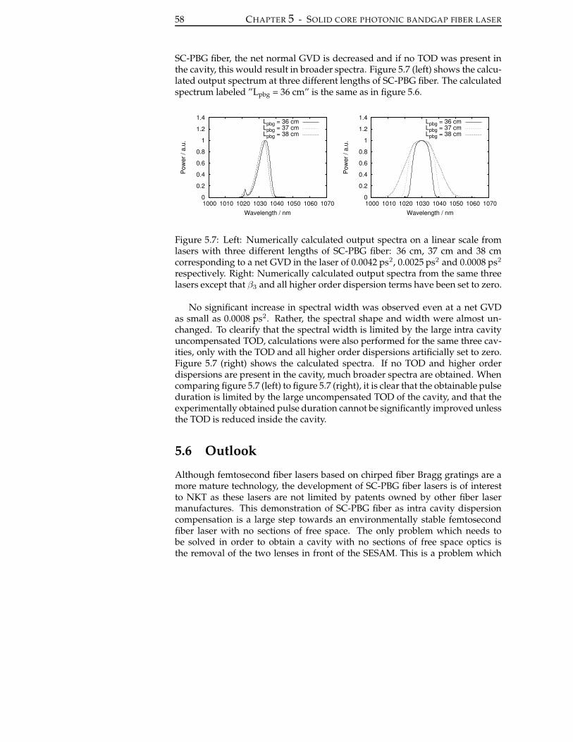
58 CHAPTER 5 - SOLID CORE PHOTONIC BANDGAP FIBER LASER
SC-PBG fiber, the net normal GVD is decreased and if no TOD was present inthe cavity, this would result in broader spectra. Figure 5.7 (left) shows the calcu-lated output spectrum at three different lengths of SC-PBG fiber. The calculatedspectrum labeled ”Lpbg = 36 cm” is the same as in figure 5.6.
0
0.2
0.4
0.6
0.8
1
1.2
1.4
1000 1010 1020 1030 1040 1050 1060 1070
Pow
er /
a.u.
Wavelength / nm
Lpbg = 36 cmLpbg = 37 cmLpbg = 38 cm
0
0.2
0.4
0.6
0.8
1
1.2
1.4
1000 1010 1020 1030 1040 1050 1060 1070
Pow
er /
a.u.
Wavelength / nm
Lpbg = 36 cmLpbg = 37 cmLpbg = 38 cm
Figure 5.7: Left: Numerically calculated output spectra on a linear scale fromlasers with three different lengths of SC-PBG fiber: 36 cm, 37 cm and 38 cmcorresponding to a net GVD in the laser of 0.0042 ps2, 0.0025 ps2 and 0.0008 ps2
respectively. Right: Numerically calculated output spectra from the same threelasers except that β3 and all higher order dispersion terms have been set to zero.
No significant increase in spectral width was observed even at a net GVDas small as 0.0008 ps2. Rather, the spectral shape and width were almost un-changed. To clearify that the spectral width is limited by the large intra cavityuncompensated TOD, calculations were also performed for the same three cav-ities, only with the TOD and all higher order dispersions artificially set to zero.Figure 5.7 (right) shows the calculated spectra. If no TOD and higher orderdispersions are present in the cavity, much broader spectra are obtained. Whencomparing figure 5.7 (left) to figure 5.7 (right), it is clear that the obtainable pulseduration is limited by the large uncompensated TOD of the cavity, and that theexperimentally obtained pulse duration cannot be significantly improved unlessthe TOD is reduced inside the cavity.
5.6 Outlook
Although femtosecond fiber lasers based on chirped fiber Bragg gratings are amore mature technology, the development of SC-PBG fiber lasers is of interestto NKT as these lasers are not limited by patents owned by other fiber lasermanufactures. This demonstration of SC-PBG fiber as intra cavity dispersioncompensation is a large step towards an environmentally stable femtosecondfiber laser with no sections of free space. The only problem which needs tobe solved in order to obtain a cavity with no sections of free space optics isthe removal of the two lenses in front of the SESAM. This is a problem which
5.7. SUMMARY 59
has been solved by other fiber laser manufactures and is primarily a questionof proper design of the SESAM. However, as only a very limited number ofSESAMs were available during this study, this last step will be left to others.
A much more serious concern is the environmental stability of the laser. Theenvironmental stability of the laser was limited by the use of non-PM fiber pig-tailed components and primarily the non-PM SC-PBG fiber. The non-PM fiberpigtailed components are easily replaceable with PM pigtailed alternatives, anda birefringent version of the SC-PBG fibers is under development at Crystal Fi-bre. Hence a environmentally stable all-fiber laser based on SC-PBG fiber fordispersion compensation and with no sections of free space will be developedat NKT-Research in the near future based on this study.
If a pulse duration significantly shorter than the 158 fs as demonstrated hereis required, either something has to be done to reduce the TOD of the SC-PBGfibers or elements with opposite sign of the TOD have to be included in the cav-ity. This is however also beyond the scope of this research. In reference [54] Ildayet al. demonstrates pulses with a duration as short as 36 fs from an ytterbiumdoped fiber laser, utilizing a bulk grating compressor for intra cavity dispersioncompensation. However, with fiber based components for dispersion compen-sation, such as e.g. chirped fiber Bragg gratings, only pulse durations in theorder of ∼ 100 fs have been obtained from ytterbium based fiber lasers.
5.7 Summary
The use of SC-PBG fiber for intra cavity dispersion compensation in a mode-locked fiber laser has been investigated. SC-PBG fiber possess a large TOD, andthis was both experientially and numerically verified to be the limiting factoron the obtainable pulse duration from fiber lasers utilizing SC-PBG fibers. Theprimary limitation was on the obtainable spectral width from the oscillator. Fur-thermore, a residual third order chirp resulted in output pulses with minimumpulse durations 15 % above the transform limit. This third order chirp was,however, demonstrated to be removable through nonlinear pulse propagationin an amplifier. As a result pulse durations down to 158 fs were demonstrated,and this is significantly shorter than what can be obtained without intra cavitydispersion compensation.

61
CHAPTER 6
Self-similar all-polarizationmaintaining environmentally stablefiber laser
This chapter presents an environmentally stable self-starting fiber laser based ona SESAM and polarization maintaining (PM) fiber pigtailed components. Thelaser was designed to operated in the self-similar regime and the laser gener-ates parabolic-like pulses. Pulse energies of 1 nJ at a repetition rate of 17 MHzand a central wavelength of 1035 nm were obtained, and the pulses were exter-nally compressible to a duration of 210 fs. Parabolic pulses are interesting fordirect amplification, and chapter 7 presents an amplifier based on amplificationof these pulses to the micro-Joule level. The experimental work of this chapterand chapter 7 were done in Jena.

62CHAPTER 6 - SELF-SIMILAR ALL-POLARIZATION MAINTAINING
ENVIRONMENTALLY STABLE FIBER LASER
6.1 Introduction
Propagation of short optical pulses with high peak powers inside optical fiberscan cause high pulse distortions and pulse break-up due to high nonlinearitiesinside the fiber. Nonlinearities are important inside mode-locked fiber lasersdue to the fact that the highest allowable total nonlinear phaseshift is usuallyof the order of π. If this intensity dependent phase shift is too high during oneround trip, the pulse cannot reproduce itself within a constant phase shift, andhence the laser output fluctuates from pulse to pulse. As illustrated in chapter 3,the laser then enters the noise-like mode-locked regime if nothing is done toprevent it. A special kind of pulse does however tolerate a larger nonlinearphase shift: pulses with a parabolic temporal profile:
a(t) = a0
(
1−(
tt0
)2)1/2
|t| ≤ t0
a(t) = 0 |t| > t0. (6.1)
The nonlinear phase shift, φNL(t) = γL|a(t)|2, accumulated by a parabolic pulse,is also parabolic and hence adds to the chirp with a linear contribution:
c(t) = −∂φNL
∂t=
2a0
t20t. (6.2)
Linear chirps are compressible by other linear dispersive elements inside anoscillator and if the pulse inside the cavity is parabolic, the laser output is nolonger limited by the nonlinear phase shift. Figure 6.1 (left) shows both a chirpedparabolic and a chirped Gaussian pulse and the contributions to their chirpsfrom a nonlinear phase shift of 2π (at the peak of the pulses). As can be seenin the figure, the contribution to the chirp from the nonlinear phase shift to theparabolic pulse is linear over the extent of pulse, whereas the chirp of the Gaus-sian pulse is only approximately linear over the central part of the pulse anddeviates in the wings.
The nonlinear phase shift is also important in amplifiers, if the pulses are tobe compressible afterwards. It was shown in reference [32] and [23] that para-bolic pulses with a linear chirp can be generated in high gain amplifiers. Suchpulses can propagate self-similarly - that is in a form preserving manner - in-side fibers with normal dispersion and high gain, even if the total nonlinearphaseshift exceeds π. As the pulse propagates, the temporal and spectral widthincreases exponentially, while maintaining a linear chirp that can be removedafterwards. The theory of parabolic pulse propagation in amplifiers will be fur-ther deepened in chapter 7. In an oscillator, the limit on the nonlinear phase shiftcan also be increased by designing the oscillator to develop parabolic pulsesand using the self-similar nature of parabolic pulse propagation. The first self-similar oscillator was demonstrated by Ilday et al. [24]. Today the largest pulseenergies from fiber oscillators are obtained from self-similar oscillators [57]. A
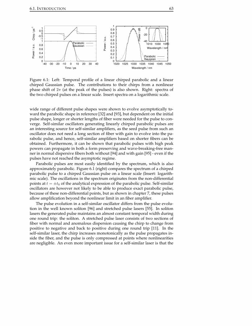
6.1. INTRODUCTION 63
0 0.2 0.4 0.6 0.8
1
-40 -30 -20 -10 0 10 20 30 40
Pow
er /
a.u.
Time / ps
ParabolicGaussian
-1-0.5
0 0.5
1
Chi
rp /
ps-1
0 0.1 0.2 0.3 0.4 0.5 0.6 0.7 0.8 0.9
1
1020 1025 1030 1035 1040 1045 1050
Pow
er /
a.u.
Wavelength / nm
ParabolicGaussian
-40
-20
0
1010 1030 1050
Pow
er /
dB
Wavelength / nm
Figure 6.1: Left: Temporal profile of a linear chirped parabolic and a linearchirped Gaussian pulse. The contributions to their chirps from a nonlinearphase shift of 2π (at the peak of the pulses) is also shown. Right: spectra ofthe two chirped pulses on a linear scale. Insert spectra on a logarithmic scale.
wide range of different pulse shapes were shown to evolve asymptotically to-ward the parabolic shape in reference [32] and [93], but dependent on the initialpulse shape, longer or shorter lengths of fiber were needed for the pulse to con-verge. Self-similar oscillators generating linearly chirped parabolic pulses arean interesting source for self-similar amplifiers, as the seed pulse from such anoscillator does not need a long section of fiber with gain to evolve into the pa-rabolic pulse, and hence, self-similar amplifiers based on shorter fibers can beobtained. Furthermore, it can be shown that parabolic pulses with high peakpowers can propagate in both a form preserving and wave-breaking-free man-ner in normal dispersive fibers both without [94] and with gain [95] - even if thepulses have not reached the asymptotic regime.
Parabolic pulses are most easily identified by the spectrum, which is alsoapproximately parabolic. Figure 6.1 (right) compares the spectrum of a chirpedparabolic pulse to a chirped Gaussian pulse on a linear scale (Insert: logarith-mic scale). The oscillations in the spectrum originates from the non-differentialpoints at t = ±t0 of the analytical expression of the parabolic pulse. Self-similaroscillators are however not likely to be able to produce exact parabolic pulse,because of these non-differential points, but as shown in chapter 7, these pulsesallow amplification beyond the nonlinear limit in an fiber amplifier.
The pulse evolution in a self-similar oscillator differs from the pulse evolu-tion in the well known soliton [96] and stretched pulse lasers [55]. In solitonlasers the generated pulse maintains an almost constant temporal width duringone round trip: the soliton. A stretched pulse laser consists of two sections offiber with normal and anomalous dispersion causing the chirp to change frompositive to negative and back to positive during one round trip [11]. In theself-similar laser, the chirp increases monotonically as the pulse propagates in-side the fiber, and the pulse is only compressed at points where nonlinearitiesare negligible. An even more important issue for a self-similar laser is that the

64CHAPTER 6 - SELF-SIMILAR ALL-POLARIZATION MAINTAINING
ENVIRONMENTALLY STABLE FIBER LASER
pulse must experience a large gain per round trip in order to take advantage ofthe spectral bandwidth of the gain medium, to shape the pulse. The net cavitydispersion should also be positive so that the pulse is always positively chirped.
The energy achievable in soliton fiber laser systems is limited to some tenpicojoules [97]. On the other hand, stretched pulse lasers with output energiesfrom tens of picojoules to some nanojoules have been reported [56, 98–100]. Self-similar pulse evolution inside mode-locked fiber lasers has recently been shownto extend the obtainable pulse energy beyond the limit found in stretched-pulselasers [57]. Therefore, the self-similar pulse regime is an interesting regime toinvestigate. Previous to the publication of our paper [V], self-similar pulses hadonly been generated from fiber lasers based on the nonlinear polarization evo-lution in the ring geometry [24]. This method does not allow for the use of PMfibers because of the walk-off between light polarized along the two axis of thefiber. Hence, environmentally stable lasers cannot be obtained with this geome-try as nonlinear polarization evolution in non-PM fibers is sensitive to environ-mentally induced changes in the birefringence of the fiber. Environmentally sta-ble fiber lasers have, however, been reported in a variety of other configurations,based on both nonlinear polarization evolution [58, 101] and saturable absorbermirrors [84]. However, as environmental instabilities in fiber lasers mainly arisefrom environmentally induced changes in the birefringence of non-PM fibers,the most natural approach is to use PM fibers with the light polarized onlyalong the slow axis. This of course eliminates the possibility of using nonlin-ear polarization evolution. In this chapter the generation of self-similar pulsesfrom a linear cavity comprising only PM fibers is demonstrated.
6.2 Cavity design
Two different cavity configurations have been investigated and self-starting self-similar pulses could be generated over a wide range of parameters such as out-put coupling, pump power and net cavity dispersion. The two different cav-ity configurations can be seen in figure 6.2. In both cases the mode-lockingmechanism is based on a semiconductor saturable absorber mirror (SESAM)and highly efficient transmission gratings have been used for intra cavity dis-persion compensation. The fiber length inside the cavity was also chosen to bethe same in the two cases and the only difference was the choice of output cou-pling. In one case (figure 6.2(a)), the output coupler was a fixed fiber pig-tailedcoupler allowing for a fiber based output. The coupler was a thin-film 30:70 PMcoupler (output coupling: 30 %) with transmission in only the slow axis. In theother case (figure 6.2(b)) the output coupler was based on a bulk polarizer anda quarter-wave plate allowing a tunable output coupling. Both cases are pre-sented here, as highest output powers were obtained from laser (b), but laser(a) had the advantage of an fiber coupled output and was used for the setup inchapter 7.
The gain medium was a 31 cm long highly ytterbium doped (∼ 300 dB/m

6.2. CAVITY DESIGN 65
HRGrating
0.31m
SM Pump
PM Yb FiberPM WDM980/1030
976nm
Compressor
Grating0.31m
SM Pump
Output
PM Yb FiberPM WDM980/1030
976nm
Compressor
Output
PBS
λ/2
λ/2 λ/2 λ/4
(a)
(b)
Passive PM Fiber
HR
PM Coupler30/70
SESAM
SESAM
Figure 6.2: The two different cavity designs: (a) with fiber output coupler and(b) with variable bulk output coupler. PM - polarization maintaining, HR - highreflection mirror, SESAM - saturable absorber mirror, PBS - polarization beamsplitter.
absorption at 976 nm) PM fiber with a mode-field diameter of 4.8 µm. The uti-lization of the minimal length of gain fiber allows to decouple gain bandwidthfiltering from the nonlinear evolution in the undoped fiber because the effect ofGVD and nonlinearity can be neglected during the amplification [24]. This fiberwas pumped through a thin-film PM WDM by a single mode diode providinga maximum output power of 400 mW at a wavelength of 976 nm. The passivefibers used in the setup were Panda 980 PM fibers with mode field diametersof ∼ 7 µm at 1035 nm and a dispersion of 0.023 ps2/m. The total fiber lengthinside the cavity was 5.6 m for both cavity designs and in both cases the lengthof the passive fiber on both sides of the gain medium was equal in order to cre-ate symmetric conditions for the pulse evolution after the gain medium in bothdirections. All the PM fibers were fusion spliced together with an estimatedpolarization extinction ratio above 37.5 dB and all fiber ends were either anglepolished or angle cleaved.
The SESAM is commercially available [60] and is based on a non-resonantdesign, using a GaAs/AlAs Bragg mirror with 27 layer pairs and 26 low tem-perature molecular beam epitaxy grown InGaAs quantum wells in front of themirror. The AR coated device has a low-intensity absorption of 45 %, a modula-tion depth of∼ 30 % and a saturation fluence of∼ 100 µJ/cm2. The recovery dy-namics of the optical excitation has been measured in a pump-probe experimentusing 200 fs pulses. The pump-probe experiment was carried out by D. Fischer

66CHAPTER 6 - SELF-SIMILAR ALL-POLARIZATION MAINTAINING
ENVIRONMENTALLY STABLE FIBER LASER
and G. Steinmeyer, MBI Berlin, Germany. The SESAM shows a bi-temporal im-pulse response with a short relaxation time of < 200 fs and a slower part of 500fs. The ratio of the fast and slow parts has been determined to 3:2.
To saturate the SESAM sufficiently a telescope was used to image the outputof the fiber onto the SESAM. To obtain self-similar pulse evolution in a SESAMbased laser, it is important to be far beyond the saturation energy, so that tem-poral shaping in the SESAM can be neglected. In chapter 8 the opposite case isexplored where a SESAM operated close to the saturation energy is the primarysource of temporal shaping.
The transmission gratings used for intra cavity dispersion compensationwere 1250 lines/mm gratings made of fused silica [102] with a high transmis-sion into first order (>95% at 1035 nm). The gratings were set up in Lithrowangle (40◦) with a grating separation of 16 mm. A half-wave plate was usedbetween the gratings and the PM fiber to ensure excitation of only the slow axis.In laser (b) an additional half-wave plate was also used to ensure excitation ofonly the slow axis of the fiber after the polarizer. If the axis of the fiber itselfis properly aligned to the grating or the polarizer, the half wave plate can beremoved resulting in an even simpler setup. With the fiber pig-tailed couplerused in laser (a), a half-wave plate was no longer necessary, as the coupler initself worked as a polarizer transmitting only light in the slow axis.
6.3 Experimental results
Special care had to be taken to align the half-wave plates to ensure excitationof only the slow axis with a high extinction ratio. It was difficult to align thewave-plates accurately in especially laser (b) as in this configuration there wasno polarization dependent loss inside the fiber. With the fiber pig-tailed cou-pler/polarizer in laser (a) it was much easier, as only one wave-plate had to bealigned. If the wave-plates were not perfectly aligned (i.e. within one degree),smaller or larger ripples on top of the spectrum could be observed.
Self-similar spectra, characterized by a parabolic top and with steep edges [24],with a FWHM between 8 and 12 nm dependent on the pump power, could beobtained with a net cavity dispersion of ∼ 0.02 ps2 from both lasers. A typicaloutput spectrum from laser (b) is shown in figure 6.3 (left), where the FWHMof the self-similar spectrum is 11.3 nm. As the pump power was increased thespectral width increased monotonically, until the threshold for double-pulsingwas reached (i.e. two pulses per round trip). The relatively large value of the netcavity dispersion of (≥ 0.02 ps2) was chosen to obtain a symmetric spectrum.
In contrast, for lower but still positive values of net cavity dispersion, broaderbut asymmetric and more structured spectra could be observed, which corre-spond to the stretched-pulse regime [57]. In the following the focus will only beon the self-similar regime.
The highest output pulse energy was obtained from laser (b), where the out-put coupling could be tuned. For a high output coupling coefficient the highest
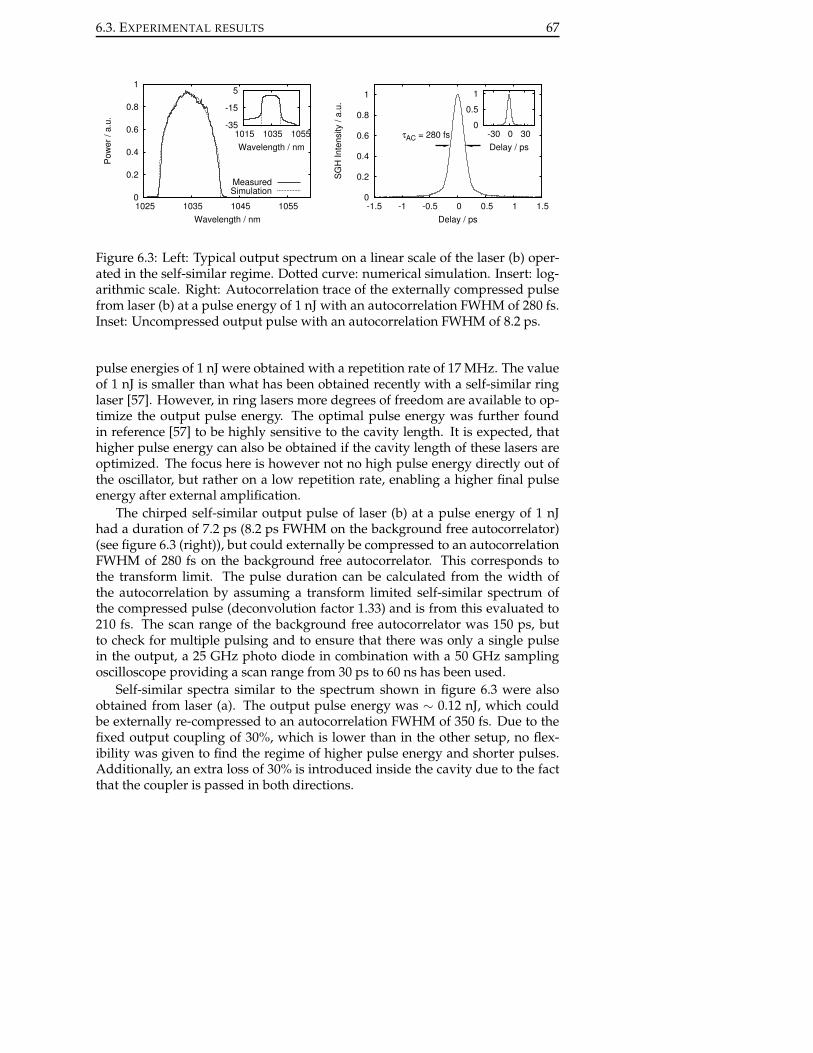
6.3. EXPERIMENTAL RESULTS 67
0
0.2
0.4
0.6
0.8
1
1025 1035 1045 1055
Pow
er /
a.u.
Wavelength / nm
MeasuredSimulation
-35
-15
5
1015 1035 1055Wavelength / nm
0
0.2
0.4
0.6
0.8
1
-1.5 -1 -0.5 0 0.5 1 1.5
SG
H In
tens
ity /
a.u.
Delay / ps
τAC = 280 fs 0
0.5
1
-30 0 30Delay / ps
Figure 6.3: Left: Typical output spectrum on a linear scale of the laser (b) oper-ated in the self-similar regime. Dotted curve: numerical simulation. Insert: log-arithmic scale. Right: Autocorrelation trace of the externally compressed pulsefrom laser (b) at a pulse energy of 1 nJ with an autocorrelation FWHM of 280 fs.Inset: Uncompressed output pulse with an autocorrelation FWHM of 8.2 ps.
pulse energies of 1 nJ were obtained with a repetition rate of 17 MHz. The valueof 1 nJ is smaller than what has been obtained recently with a self-similar ringlaser [57]. However, in ring lasers more degrees of freedom are available to op-timize the output pulse energy. The optimal pulse energy was further foundin reference [57] to be highly sensitive to the cavity length. It is expected, thathigher pulse energy can also be obtained if the cavity length of these lasers areoptimized. The focus here is however not no high pulse energy directly out ofthe oscillator, but rather on a low repetition rate, enabling a higher final pulseenergy after external amplification.
The chirped self-similar output pulse of laser (b) at a pulse energy of 1 nJhad a duration of 7.2 ps (8.2 ps FWHM on the background free autocorrelator)(see figure 6.3 (right)), but could externally be compressed to an autocorrelationFWHM of 280 fs on the background free autocorrelator. This corresponds tothe transform limit. The pulse duration can be calculated from the width ofthe autocorrelation by assuming a transform limited self-similar spectrum ofthe compressed pulse (deconvolution factor 1.33) and is from this evaluated to210 fs. The scan range of the background free autocorrelator was 150 ps, butto check for multiple pulsing and to ensure that there was only a single pulsein the output, a 25 GHz photo diode in combination with a 50 GHz samplingoscilloscope providing a scan range from 30 ps to 60 ns has been used.
Self-similar spectra similar to the spectrum shown in figure 6.3 were alsoobtained from laser (a). The output pulse energy was ∼ 0.12 nJ, which couldbe externally re-compressed to an autocorrelation FWHM of 350 fs. Due to thefixed output coupling of 30%, which is lower than in the other setup, no flex-ibility was given to find the regime of higher pulse energy and shorter pulses.Additionally, an extra loss of 30% is introduced inside the cavity due to the factthat the coupler is passed in both directions.

68CHAPTER 6 - SELF-SIMILAR ALL-POLARIZATION MAINTAINING
ENVIRONMENTALLY STABLE FIBER LASER
To make sure that the lasers operates in the self similar regime some inspec-tions have to be made. First of all, the spectrum should of course exhibit a self-similar shape, which is fulfilled in our case. Secondly, an important conditionfor self-similar evolution is that the pulse is always positively chirped insidethe cavity and with a minimum pulse duration after the intra cavity gratingsjust before entering the fiber [57]. The negative dispersion given by the grat-ing pair used for external compression (∼ −0.36 ps2 (double pass)) was higherthan that of the pair used inside the cavity. In addition, only half the length ofintra cavity fiber is passed before the pulse is coupled out. This indicates thatthe pulse is still highly positively chirped before entering the fiber after the in-tra cavity grating pair. As the dispersion from this point on inside the cavity ispositive until the pulse again reaches the intra cavity gratings, this point mustbe a minimum point. As an additional verification, a numerical simulation ofthe cavity was carried out. Each segment was treated separately by solving thenonlinear Schrodinger equation with the parameters of our experimental setup.In figure 6.3 the simulated spectrum can be seen to be in good agreement withthe measured spectrum. In the simulation the pulse exhibits self-similar pulsepropagation [57] and is always positively chirped.
In both configurations the laser was self-starting and immediately jumpedback into the same mode-locked state without any external perturbations if, forinstance the laser was switched off and back on again. Furthermore, the useof PM fibers made the laser stable toward environmentally induced changes tothe birefringence of the fiber. The fibers could be twisted and moved aroundwhile maintaining a stable mode-locked output. This was verified by observinga uniform train of pulses using a fast photo diode and an analog scope.
6.3.1 Bound states
As mentioned above, it is important to verify, that only a single pulse residesinside the cavity. This is especially true in long fiber lasers or at high intra cavityaverage powers, where the power can be distribute over two or more pulses.This occurs if two pulses result in a smaller loss, and hence a more attractivesolution to the cavity, or if the nonlinear phaseshift is so high, that a single pulsebreaks up [103, 104]. The resulting smaller pulse energy per pulse is usually anunwanted effect. In general, these pulses are randomly separated, but undercertain conditions these pulses can be regularly spaced in the cavity. Two differ-ent scenarios can happen. If n pulses coexist in the cavity simultaneously, theycan either be separated by TR/n where TR is the round trip time, and hence cre-ate a pulse train with a repetition rate n times larger than the fundamental. Thisis called harmonic mode-locking. Alternatively they can be spaced very closelytogether with a fixed separation which is much smaller than TR. This is calledbound-state mode-locking. The later case is the most difficult to detect at firstsight, as the pulses can be difficult to resolve with ordinary oscilloscopes andphoto diodes.
Laser (a) was limited to a lower pulse energy compared to laser (b) by the

6.3. EXPERIMENTAL RESULTS 69
0
0.2
0.4
0.6
0.8
1
1.2
1025 1030 1035 1040 1045 1050 1055
Pow
er /
a.u.
Wavelength / nm
Single pulseBound states
0
0.5
1
1034 1034.8
∆λ = 0.19 nm
0
0.2
0.4
0.6
0.8
1
1.2
-60 -40 -20 0 20 40 60
SG
H In
tens
ity /
a.u.
Delay / ps
18.7 ps
CompressedUncompressed
Figure 6.4: Left: Output spectrum from the laser in the single pulse and thebound stats regimes. Insert: zoom on the spectral fringes. Right: Autocorre-lation of the laser output in the bound state regime (before and after externalcompression).
onset of bound-state lasing. At a pump power of about 94 mW, stable self-starting single pulse mode-locking was observed. If the pump power was nowincreased, the laser switched into a new regime of operation, where two closelybound pulses circulated inside the cavity. At a typical pumping power of 125mW the two bound states were self-starting - i.e. if the laser beam inside thecavity was blocked and afterwards unblocked, the laser jumped right back intothe same mode-locking state. The transition was observable both spectrally andtemporally. Figure 6.4 (left) shows the output spectrum of laser (a) in the boundstate and in the single pulse regime. The spectral width decreased slightly inthe bound state regime due to the lower pulse energy per pulse, and is stronglymodulated, which is a direct consequence of the a precise phase relationshipmaintained between the two pulses. Note that the exact modulation depth can-not be found due to the limited resolution of the spectrum analyzer (0.05 nm),but is believed to be larger than the measured 80 %. The insert of figure 6.4 (left)shows a zoom in on the spectral fringes. The fringes correspond to a two-waveinterference pattern with 0.19 nm period.
The autocorrelation traces of both the compressed and uncompressed twobound states can be seen in figure 6.4 (right). The temporal separation, d, of thetwo pulses was measured to 18.7 ps in correspondence with the spectral mod-ulation period (∆λ = λ2
c·d ), and the duration of the uncompressed pulses was8.3 ps. After external compression a pulse duration of 248 fs (410 fs autocorrela-tion FWHM) was obtained. The slightly longer pulse duration is in correspon-dence with the slightly narrower spectrum. In the two bound state regime thepulse energy per pulse was 70 pJ. If the pump power was further increased,regimes of three and even four bound states were obtained.

70CHAPTER 6 - SELF-SIMILAR ALL-POLARIZATION MAINTAINING
ENVIRONMENTALLY STABLE FIBER LASER
6.4 Outlook
Besides the demonstration of a self-starting environmentally stable fiber laserconstructed from PM fibers only, the truly interesting aspect about the presentedlaser is its output spectral shape and especially the amplification of this outputbeyond the nonlinear limit in a fiber amplifier. This will be the scope of thenext chapter. As the central wavelength of the laser was 1034 nm, the laser isa suitable candidate for amplification in short large-mode-area ytterbium fiberamplifiers and the spectral width of the laser is also almost ideal, as broaderspectra can experience significant spectral gain narrowing in the amplifier.
6.5 Summary
In summary, it has been experimentally demonstrated that a self-starting self-similar oscillator can be obtained with a linear cavity where a SESAM is used asthe nonlinear mode-locking mechanism. Further, the oscillator was intrinsicallyenvironmentally stable, as only PM fibers were used. Pulses with an energy of1 nJ at a repetition rate of 17 MHz were obtained, and the output pulse durationwas 7.2 ps, but could be externally compressed to a pulse duration of 210 fs.

71
CHAPTER 7
Microjoule-level allpolarization-maintainingfemtosecond fiber source
Direct amplification of parabolic pulses from an environmental stable passivelymode-locked fiber oscillator is presented here. The pulses are amplified in anYb-doped single-polarization photonic crystal fiber and the special pulse shapeallows for the generation of high quality femtosecond pulses beyond the non-linear limit. The system delivers 240 fs pulses with a pulse energy of 1.2 µJ(21 W average power) at a repetition rate of 17 MHz and central wavelength of1035 nm in a linearly polarized beam with diffraction-limited quality.

72CHAPTER 7 - MICROJOULE-LEVEL ALL POLARIZATION-MAINTAINING
FEMTOSECOND FIBER SOURCE
7.1 Introduction
Due to the outstanding heat dissipation capabilities of a rare-earth-doped fibers,average power scaling of fiber amplifiers is a straightforward problem, whichmakes a fiber amplifier system interesting for e.g. fast material processing [13].Furthermore, nonlinear effects during amplification can be greatly reduced bythe application of Yb-doped low-nonlinearity photonic crystal fibers with ex-tended single-mode cores compared to step index fibers [105] and absorptionlength of only some ten centimeters [106]. Especially, the possibility of makingvery short fiber amplifiers makes ytterbium a better choice over e.g. erbium.The problem with erbium is that the doping concentration in the fiber is limitedby concentration quenching due to cluster formation [107]. Hence longer fibersare needed to obtain the same total gain, but longer fibers also result in a largernonlinear phase shift accumulated by the pulse. In general, the nonlinearity ofa fiber amplifier can be reduced by either decreasing its length or by increas-ing its core size. The core size in step index fibers is limited by higher ordertransverse modes. Step index fibers are only single mode (i.e. only supportinga single transverse mode) above a specific wavelength - the cut off wavelength.If the fiber is scaled in order to increase the core size, the cut off wavelengthwill also move towards higher wavelengths and eventually above the desiredlasing wavelength. The result is an output which is no longer diffraction lim-ited. Photonic crystal fibers (PCFs) can be designed to be endlessly single mode(i.e. supporting only a single mode at all wavelengths) by increasing the air fillfraction of the cladding, and hence increasing the index step between the coreand the average index of the cladding [108]. Endlessly single mode fibers can inprinciple be scaled to have any core size. However, a further limit is set by thebend losses of the fiber. Like conventional fibers, PCFs exhibit a bend loss edgeat long wavelengths. The reason for this is that the mode extends further intothe cladding at longer wavelengths, resulting in a more weakly guided modethat will suffer a greater perturbation in response to bending. In addition tothis PCFs also have a short wavelength bend loss edge due to the wavelengthdependent effective index in the cladding [108]. As the fiber is scaled, the lowbend loss edge also moves towards higher wavelengths. A solution to this prob-lem was introduced in reference [106] where the fiber was simply drawn into arod with almost zero flexibility. On the practical side, however, another prob-lem arises with increasing core size. As the core size increases, it is increasinglydifficult to polish the core to be entirely scratch free.
Compact and environmentally stable high energy and high average powerultra-short pulse laser sources have many applications. Examples are micro ma-chining, marking, eye surgery (ophthalmology), index modification in trans-parent materials (waveguide writing) and frequency conversion. In terms ofcompactness, cost, reliability and ease of operation a fiber based laser system isthe predestined laser architecture. Fiber based short-pulse oscillators have beendemonstrated to be an ideal candidate for compact femtosecond laser sources [56].

7.1. INTRODUCTION 73
However, the pulse energy from fiber lasers is fundamentally limited by thenonlinear phase shifts accumulated during propagation through the fibers in-side the cavity [57]. Hence, to reach pulse energies sufficient for most applica-tions, the laser has to be amplified.
The pulse energy is also limited in amplifiers by the nonlinearities. Depend-ing on the pulse shape, a large nonlinear phase shift can result in a pulse whichcannot be compressed to the transform limit with linear dispersive elementslike gratings and hence the pulse quality degrades. Nonlinear effects also in-troduce other pulse quality degrading problems, like wave-breaking where thepulse breaks up into several pulses [94]. Wave-breaking is a consequence ofdifferent frequency components of chirped pulses, catching up with other fre-quency components due to different group velocities and happens to pulseswith non-monotonically varying chirps [94]. Further problems arise throughthe generation of stimulated Raman scattering [109], which decreases and limitsthe obtainable pulse energy and also increases the noise on the pulse. As men-tioned in chapter 6 the final amplified pulse quality can be highly increased, ifthe input pulse has a parabolic shape. The reason for this is the shape of thenonlinear phase, which is also parabolic according to the intensity profile of thepulses [32]. In the high power limit (see equation 7.3 below), the pulse willremain a parabolic shape with linear chirp also after amplification [95].
So far amplified mode-locked fiber laser systems suffer from the lack of sta-bility of non-polarization maintaining (non-PM) components. As demonstratedin chapter 6 environmentally stable fiber lasers can be constructed using polari-zation maintaining (PM) fibers. However, if a linearly polarized environmen-tally stable amplified output is desired, all stages including the amplifier shouldbe PM. It was shown in reference [110] that a single polarization property couldbe added directly to low nonlinearity PCFs, which increases stability and furtherreduces the complexity of the setup by reducing polarization control [110].
In terms of average powers, impressive results from femtosecond fiber am-plifier systems have already been obtained using non-polarization maintaininglow-nonlinearity fibers in chirped pulse amplification systems [111] and in am-plifiers, where a parabolic pulse is created during amplification and thereforeadditional pulse stretching is not necessary [112]. The nonlinearity in the ampli-fication stage can of course be greatly reduced by incorporating temporal pre-stretching of the pulse using e.g. bulk gratings before launching it into the am-plifier. 1.8 µJ 220 fs pulses at 1040 nm with a repetition rate of 73 MHz wereobtained in reference [111] by applying this approach, and 100 µJ at a repetitionrate of 200 kHz was obtained in reference [14], but the bulk grating separationof 1 m in these systems, doesn’t exactly make them compact. More compactprestretching schemes have also been demonstrated. 6.5 µJ 940 fs pulses wereobtained at 1558 nm in reference [113] after prestretching the pulses to 720 pswith the use of a chirped fiber Bragg grating, subsequent amplification in anlarge-mode area Er/Yb-doped fiber and recompression with an bulk gratingcompressor. Direct amplification without prestretching is, however, preferableas it simplifies the setup, and large grating separations can be avoided.

74CHAPTER 7 - MICROJOULE-LEVEL ALL POLARIZATION-MAINTAINING
FEMTOSECOND FIBER SOURCE
Especially, the amplification of parabolic pulses allows for the realizationof high peak powers without any significant degradation of the recompressedpulse quality. If the pulse entering the amplifier is already parabolic, it is notnecessary to take special care of the parabolic pulse evolution in the followingamplifier stages in comparison to references [32, 112]. Consequently, the combi-nation of an oscillator delivering parabolic pulses and a polarization-maintaininglow-nonlinearity fiber seems to provide an easy way for high-energy linearlypolarized femtosecond pulse generation. In this chapter the theory behind pa-rabolic amplifiers and amplification of parabolic pulses will be introduced, fol-lowed by the first demonstration of direct amplification of parabolic pulses froma self-similar oscillator [VI]. The setup was further the first demonstration ofamplification of an environmentally stable femtosecond fiber laser in an PM andsingle polarization amplifier to the microjoule level without significant pulsequality degradation.
7.2 Theory
To understand the difference between direct amplification of parabolic pulsesand self-similar amplifiers, the theory of self-similar amplifiers is first intro-duced. Fermann et al. [32] were the first to introduce the concept of self-similarpulse evolution in fiber amplifiers. A solution u = u(x, t) of a nonlinear par-tial differential equation is called self-similar if the knowledge of u at time t0 issufficient to obtain u for all t > t0 by a suitable rescaling.
Fermann showed that parabolic pulses are exact asymptotic solutions to thenonlinear Schrodinger equation (NLSE):
∂a
∂z= −i
1
2β2
∂2a
∂t2+ iγ|a|2a +
g
2a, (7.1)
with constant gain, g (both spectrally and longitudinal). The analytical theorywas extended to include longitudinal gain variations, g(z), in reference [114]and further to include variations in β2(z) and γ(z) in reference [115]. However,the inclusion of non-constant g, β2 and γ increases the complexity of the analysisand the essential physics can be understood from the simpler case. The onlyconditions that have to be fulfilled for self-similar pulse propagation are β2γ > 0and g > 0, which restrict the theory to normally dispersive fiber amplifiers, suchas e.g. Yb-doped fiber amplifiers.
Independently of the initial pulse shape, any pulse will evolve asymptot-ically into a similariton - i.e. a pulse with a parabolic intensity profile and alinear positive chirp:
a(z, t) = a0(z)(
1−(
tt0(z)
)2)1/2
exp(iφ(z, t)) |t| ≤ t0(z)
a(z, t) = 0 |t| > t0(z), (7.2)
7.2. THEORY 75
where
a0(z) =1
2(gEIN )
13 (
2
γβ2)
16 exp(
gz
3),
is the amplitude of the parabolic pulse,
t0(z) = 3g−23 (
γβ2EIN
2)
13 exp(
gz
3),
is the tFWHM /√
2 width of the pulse, and
φ(z, t) = φ0 +3γ
2ga0(z)− g
6β2t2,
the phase of the pulse. EIN is the input pulse energy, and the asymptotic solu-tion only depends on this and on the amplifier parameters. The energy of theparabolic pulse is E(z) = 4
3a0(z)2t0(z). The linear chirp of the pulse is given by:
δω(t) = −∂φ(z, t)
∂t=
g
3β2t ≡ C · t.
An approximate analytical solution of the pulse spectrum can also be calcu-lated [114]:
|a(z, ω)|2 ' 3γa20
g exp( 23gz)
(
1−(
ωω0(z)
)2)
|ω| ≤ ω0(z)
|a(z, ω)|2 = 0 |ω| > ω0(z),
with the ωFWHM/√
2 width given by ω0(z) = C · t0(z) = g3β2· t0(z). The spec-
trum is also approximately parabolic [114] with a linear spectral chirp, and theapproximation is good for large chirps, C, whereas the spectrum resembles thatof a sinc function with many side-lobes if C = 0. Both the pulse energy, andthe temporal and the spectral width of the pulse increase exponentially in theamplifier. The temporal and spectral intensity profile of a parabolic pulse canbee seen in figure 7.1.
The generation of similaritons in optical fiber amplifiers have potential wide-ranging applications in many areas of current optical technology, as the outputpulses have a well defined linear chirp even in the presence of input pulse dis-tortions. Furthermore, all the energy of the input pulse is transfered into theparabolic pulse, as opposed to the generation of solitons, where the remain-ing energy above the soliton energy is shed off into a continuum. The intrinsicresistance to wave-breaking of parabolic pulses allows the scaling of the fiberamplifiers to higher-power regimes and the linear chirp facilitates efficient com-pression. The only issue of self-similar amplification is the propagation lengthover which a specific input pulse converges to the asymptotic solution.
To illustrate the asymptotic convergence towards a parabolic pulse, a cal-culation of an Yb-amplifier has been made by solving the NLSE numerically

76CHAPTER 7 - MICROJOULE-LEVEL ALL POLARIZATION-MAINTAINING
FEMTOSECOND FIBER SOURCE
0
0.2
0.4
0.6
0.8
1
-25 -20 -15 -10 -5 0 5 10 15 20 25
Pow
er /
a.u.
Time / ps
0 0.1 0.2 0.3 0.4 0.5 0.6 0.7 0.8 0.9
1
1000 1010 1020 1030 1040 1050 1060
Pow
er /
a.u.
Wavelength / nm
Figure 7.1: Left: Calculated temporal intensity profile of a parabolic pulse witht0 = 10 ps and C = 0.888 ps−2. Right: spectral profile of the same pulse with anapproximate parabolic shape.
with realistic parameters. The length of the amplifier was chosen to 8 m with aconstant gain, g = 0.69 m−1, corresponding to a total gain of 30 dB. The non-linear coefficient was set to γ = 3.5 · 10−3 (m W)−1, and the dispersion was setto β2 = 0.023 ps2/m (corresponding to coefficients of a fiber with mode-fielddiameter (MFD) = 7 µm). The input pulse energy was 100 pJ, correspondingto an output pulse energy of 100 nJ. Three different unchirped Gaussian pulseswith durations: 100 fs, 500 fs and 5 ps were used as input. In figure 7.2 theRMS temporal duration of the pulses vs. propagation distance in the amplifieris compared to the asymptotic limit.
0.01
0.1
1
10
0 1 2 3 4 5 6 7 8
Wid
th /
ps (<
<t2 >-
<t>2 >1/
2 )
Propagation length / m
Asymptotic0.1ps0.5ps
5ps
Figure 7.2: Calculated RMS temporal duration vs. propagation vs. distance inthe amplifier for three different unchirped Gaussian input pulses: 100 fs, 500 fsand 5 ps.
The temporal duration of the pulses always converges towards the asymp-totic solution. However the distance over which the pulses reach the asymp-

7.2. THEORY 77
totic solution is very dependent on the input pulse duration. This is even moreclearly seen if the output temporal and spectral intensity profiles are comparedto the asymptotic solution (see figure 7.3).
0
0.2
0.4
0.6
0.8
1
-20 -15 -10 -5 0 5 10 15 20
Pow
er /
a.u.
Time / ps
Asymptotic0.1ps0.5ps5.0ps
0
0.2
0.4
0.6
0.8
1
1.2
960 980 1000 1020 1040 1060 1080 1100
Pow
er /
a.u.
Wavelength / nm
Asymptotic0.1ps0.5ps5.0ps
Figure 7.3: Left: temporal output intensity profile for three different inputpulses, compared to the asymptotic solution. Right: spectral output intensityprofile compared to the asymptotic solution.
From the output spectrum (figure 7.3 (right)) it is clear that both the 100 fsand 5 ps pulses have not yet entered the parabolic regime. For a given amplifierand input pulse energy, an optimal input pulse duration for fast convergencecan be found by evaluating the similariton parameters at z = 0. With the ampli-fier parameters used in the calculation and the input pulse energy, the optimalinput duration is:
t0(0) = 3g−23 (
γβ2EIN
2)
13 = 526 fs,
In agreement with the optimal input duration the pulse with the duration of500 fs was the only one to come close the asymptotic solution. Another impor-tant property was also observed from the calculations: the higher total gain inthe amplifier, the easier it is to reach the parabolic regime. However in practicehigh gains are limited in an amplifier by amplified spontaneous emission (ASE).
As the theory of self-similar pulse amplifiers is based on a simplified NLSEwhere e.g. spectral dependence on the gain and other nonlinear effects suchas stimulated Raman scattering (SRS) have been neglected, the theory breaksdown when these effects become important. The limit set by these effects onthe obtainable pulse energy from self-similar amplifiers was calculated in refer-ence [109]. If the gain per meter is high then shorter fiber lengths are necessary.However, for shorter fiber lengths the dispersion becomes less dominant andthe spectral width of the asymptotic solution broadens. Hence, the limit in highgain amplifiers was found to be set by the finite bandwidth of the gain medium.On the other hand, in longer amplifiers with lower gain per meter the limit setby the generation of SRS is reached earlier. An optimal gain value can be found
78CHAPTER 7 - MICROJOULE-LEVEL ALL POLARIZATION-MAINTAINING
FEMTOSECOND FIBER SOURCE
in between these two limits, depending on the input pulse energy. For an Yb-doped amplifier with a gain bandwidth of 10.8 THz (38.2 nm) and a dispersionof β2 = 0.020 ps2 and with an input pulse energy of 1 nJ, the optimal gain re-sulting in maximum output pulse energy was calculated to 3.9 dB/m [109]. Themaximum output pulse energy does, however, still scale linearly with the modefield area (MFA) of the fiber. For a fiber with MFA of 700 µm2 (equal to theMFA of the fiber used in the experiments below), the maximum output pulseenergy was calculated to <0.5 µJ. Hence, if larger pulse energies from an ampli-fier fiber with given dimensions are to be obtained alternative methods have toconsidered, and one alternative is the direct amplification of parabolic pulses.
The theory of parabolic pulses was first introduced in 1993 by Anderson etal. [94], where they showed that parabolic pulses are a form invariant solutionto the NLSE with zero gain, g = 0, and in the high power limit:
β2
2|a|∣
∣
∣
∂2|a|∂t2
∣
∣
∣<< γ|a|2. (7.3)
Other well known examples of form invariant pulse are the soliton in theanomalous dispersion regime, β2 < 0, and Gaussian pulses in the dispersiveonly regime, γ = 0. The theory of parabolic pulses was extended in refer-ence [95] to include a NLSE with nonzero gain. Under the assumption of equa-tion 7.3, three differential equations for the parameters of the parabolic pulse(equation 7.2) can be derived:
∂2t0∂z2
=3
2
EINγβ2
t20(z)exp(gz) (7.4)
C(z) =1
β2
1
t0(z)
∂t0∂z
(7.5)
|a0(z)|2 =3
4
EIN
t0(z)exp(gz) (7.6)
From the first differential equation t0(z) can be numerically calculated from theinitial conditions t0(0) and (∂t0/∂z)z=0 = β2C(0)t0(0), and from t0(z) the pa-rameters, C(z) and |a0(z)|2 can be calculated.
While the output pulses are still parabolic pulses, the output pulse differsfrom the self-similar solution, as it now also depends on the input pulse parame-ters, t0(0) and C(0). The property that any pulse (i.e. also a parabolic pulse) willeventually evolve into the asymptotic solution if the amplifier is long enoughis still fulfilled, even though it is less apparent. To illustrate this, equations 7.4-7.6 were solved with the same amplifier parameters as in the previous example(figure 7.2). This time three different parabolic input pulses were chosen. Theinput pulse energy was set to 1 nJ for all pulses and the spectral width wasfixed to λ0(0) = 2πc
λ2 ω0 = 5 nm, as in figure 7.1 (right). Only the pulse dura-tion, t0(0), was varied: 1 ps, 5 ps and 10 ps. The evolution of the parameters,t0(z) and λ0(z) vs. amplification distance for the three pulse are compared to
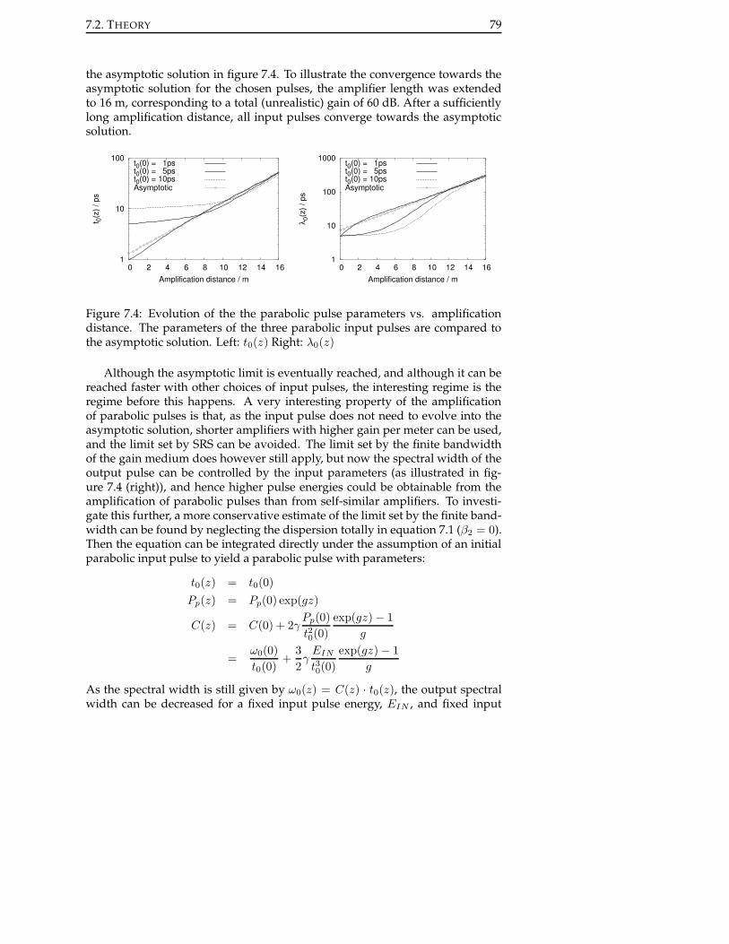
7.2. THEORY 79
the asymptotic solution in figure 7.4. To illustrate the convergence towards theasymptotic solution for the chosen pulses, the amplifier length was extendedto 16 m, corresponding to a total (unrealistic) gain of 60 dB. After a sufficientlylong amplification distance, all input pulses converge towards the asymptoticsolution.
1
10
100
0 2 4 6 8 10 12 14 16
t 0(z
) / p
s
Amplification distance / m
t0(0) = 1pst0(0) = 5pst0(0) = 10psAsymptotic
1
10
100
1000
0 2 4 6 8 10 12 14 16
λ 0(z
) / p
s
Amplification distance / m
t0(0) = 1pst0(0) = 5pst0(0) = 10psAsymptotic
Figure 7.4: Evolution of the the parabolic pulse parameters vs. amplificationdistance. The parameters of the three parabolic input pulses are compared tothe asymptotic solution. Left: t0(z) Right: λ0(z)
Although the asymptotic limit is eventually reached, and although it can bereached faster with other choices of input pulses, the interesting regime is theregime before this happens. A very interesting property of the amplificationof parabolic pulses is that, as the input pulse does not need to evolve into theasymptotic solution, shorter amplifiers with higher gain per meter can be used,and the limit set by SRS can be avoided. The limit set by the finite bandwidthof the gain medium does however still apply, but now the spectral width of theoutput pulse can be controlled by the input parameters (as illustrated in fig-ure 7.4 (right)), and hence higher pulse energies could be obtainable from theamplification of parabolic pulses than from self-similar amplifiers. To investi-gate this further, a more conservative estimate of the limit set by the finite band-width can be found by neglecting the dispersion totally in equation 7.1 (β2 = 0).Then the equation can be integrated directly under the assumption of an initialparabolic input pulse to yield a parabolic pulse with parameters:
t0(z) = t0(0)
Pp(z) = Pp(0) exp(gz)
C(z) = C(0) + 2γPp(0)
t20(0)
exp(gz)− 1
g
=ω0(0)
t0(0)+
3
2γ
EIN
t30(0)
exp(gz)− 1
g
As the spectral width is still given by ω0(z) = C(z) · t0(z), the output spectralwidth can be decreased for a fixed input pulse energy, EIN , and fixed input

80CHAPTER 7 - MICROJOULE-LEVEL ALL POLARIZATION-MAINTAINING
FEMTOSECOND FIBER SOURCE
spectral width ω0(0) by increasing t0(0). The output spectral width can hencebe controlled to less than the spectral width of the gain medium. If t0(0) is suf-ficiently large, the regime of chirped pulse amplification is of course reached,where the nonlinearities can be neglected. However, the focus is here on muchsmaller input pulse durations where the pulse still experiences a significant non-linear phase shift in the amplifier.
To further illustrate the strengths of parabolic pulse amplification, the exper-imental results from the amplification of the oscillator presented in chapter 6 arenow presented.
7.3 Experimental setup
The µJ-level all-polarization-maintaining (PM) femtosecond fiber laser sourceconsists of the environmentally stable and self-starting ytterbium-doped fiberoscillator, a polarization-maintaining pre-amplifier, a single-polarization fiberpower-amplifier and a transmission grating compressor. The experimental setupis shown in figure 7.5. For the amplifier system the oscillator with the fiber-pigtailed 30/70 coupler was used (figure 6.2). The pre-amplifier consisted of aWDM and a 0.55 m PM Yb-doped single-mode fiber with identical fiber charac-teristics as the fiber used in the oscillator. The pre-amplifier was spliced to theoscillator with an fiber-pigtailed isolator in between. Between the pre-amplifierand the power-amplifier a bulk isolator was used for isolation. After the poweramplifier the output was directed towards the Grating compressor with a dichroicmirror reflecting at 1034 nm and transmitting at 976 nm. A bulk isolator was alsoused after the power amplifier. The power-amplifier was pumped with a multi-mode 976 nm pump. The pump was fiber pigtailed to a 400 µm multi-modefiber. The pre-amplifier was pumped with a 300 mW single mode fiber-pigtailedpump diode. Aspheric lenses were used to couple light into the power ampli-fier. The grating compressor consisted of a pair of transmission gratings withhigh transmission [102].
Output
Isolator 75W MM Pump976nm1.2m PM Double clad Yb fiber
CompressorGrating
976nmSM Pump
PM Isolator
PM WDM
0.55m PM YbOscillator
All−PM
Isolator
Figure 7.5: Schematic setup of the Microjoule-level all-polarization maintainingfemtosecond fiber laser system (PM: polarization maintaining, SM: single mode,MM: multi mode, WDM: wavelength division multiplexer).

7.4. EXPERIMENTAL RESULTS 81
Figure 7.6: SEM image of the polarizing low-nonlinearity Yb-doped PCF.
The power amplifier consists of an 1.2 m long ytterbium-doped single polari-zation single-mode double-clad PCF [110] shown in figure 7.6. This fiber com-prises index-matched stress-applying elements (SAP) as part of the photoniccladding. The proximity of the SAP to the core ensures high differential stress,and thus high birefringence. Additionally due to the index matching of theSAP array to the air-hole cladding, the light is confined by both parts of thephotonic cladding: the air holes and the index matched regular array of SAPs.Furthermore, the amount of birefringence is enough to split two polarizationstates of the weakly guided fundamental mode so that the effective index of onepolarization is below the cladding index. This results in a single-polarizationlarge-mode-area fiber in a certain wavelength range, which is determined by thedesign and lies within the amplification bandwidth of Ytterbium in the presentcase. The MFA of 700 µm2 is larger than that of any step-index single-modefiber. The pump cladding is formed by an air-cladding outside the inner pho-tonic cladding and has a diameter of 170 µm and a NA of 0.6. This structure hasa pump light absorption of 14 dB/m.
The power amplifier fiber was angle polished at an angle of 4◦ in order tosuppress lasing on the ends. The fiber was further mounted with a glass to glassindexed matched interface in order to avoid melting the fiber with non-guidedpump light.
7.4 Experimental results
The parabolic output spectrum from the oscillator had a FWHM of 12.1 nm at afixed maximum output energy of 0.12 nJ. The spectrum from the oscillator canbe seen in figure 7.7 (left). The chirped parabolic output pulses had a pulse du-ration of 7.2 ps (FWHM), but could externally be compressed to a pulse durationof 260 fs. The output of the oscillator (about 2 mW average power) was ampli-fied to 50 mW and due to the additional fiber length the pulses were stretched to

82CHAPTER 7 - MICROJOULE-LEVEL ALL POLARIZATION-MAINTAINING
FEMTOSECOND FIBER SOURCE
-80
-60
-40
-20
0
20
1010 1020 1030 1040 1050
Pow
er /
dB
Wavelength / nm
OscillatorPre-amplifier
Power-amplifier
0
0.2
0.4
0.6
0.8
1
-4 -3 -2 -1 0 1 2 3 4
SH
G In
tens
ity /
a.u
Delay / ps
τAC = 320 fs
Figure 7.7: Left: Output spectrum from the oscillator, the pre-amplifier and thepower-amplifier. Right: Autocorrelation after external compression at maxi-mum amplification.
0
5
10
15
20
25
30
35
0 5 10 15 20 25 30 35 40 45 50
Oup
ut p
ower
/ W
Launched pump power / W
Slope efficiency: 72 %
Figure 7.8: Output power of the power-amplifier vs. launched pump power.
10 ps (FWHM). After direct pre-amplification, these parabolic pulses were am-plified in the single-polarization ytterbium-doped PCF to the µJ level withoutany further temporal stretching.
The output power characteristic is shown in figure 7.8. Up to 29 W aver-age power with a slope efficiency of 72 % was obtained at a launched averageseed power of ∼ 30 mW. The polarization extinction ratio was as high as 24 dB(1:250) even at the highest power level. The output spectra of the pre- and mainamplifier are also shown in figure 7.7 (left). The influence of self-phase modu-lation by the slight spectral broadening and modulation can be seen. However,the recompressed pulse quality was almost unaffected by the imposed nonlin-ear phase. The grating separation in the grating compressor was just ∼ 2 cmand the throughput efficiency was 73 % resulting in 21 W of recompressed av-erage power. The measured autocorrelation is shown in figure 7.7 (right). Theautocorrelation width was 320 fs corresponding to 240 fs pulse duration (de-convolution factor of 1.33). Consequently, the pulse peak power was as highas 5 MW after compression. The slight reduction in pulse duration compared

7.4. EXPERIMENTAL RESULTS 83
0
0.2
0.4
0.6
0.8
1
-1 -0.5 0 0.5 1
Pow
er /
a.u.
Time / ps
Transform limited parabolicParabolicGaussian
0 0.1 0.2 0.3 0.4 0.5 0.6 0.7 0.8 0.9
1
-1 -0.5 0 0.5 1
Pow
er /
a.u.
Time / ps
30dB33dB36dB
Figure 7.9: Calculated output pulses after amplification and subsequent com-pression. Left: an initial parabolic and an initial Gaussian pulse with the samecharacteristics as the pulse in the experiment. For comparison a transform lim-ited parabolic pulse is also shown (filled circles). Right: amplification of theparabolic pulse at three different total gains in the amplifier.
to the oscillator was made possible by the bandwidth enhancement in the am-plification stages. At the highest power levels wings in the autocorrelation aredeveloping, however, they contain just a minor part of energy (compare e.g. tothe calculations below (figure 7.9)). To validate that improved pulse quality wasindeed obtained as a result of parabolic shaped pulses and in spite of the devel-opment of these wings, the accumulated nonlinear phase shift in the amplifiercan be calculated:
φNL = γ
∫ L
0
|a(z, t = 0)|2dz (7.7)
If φNL is below 1 a linear propagation is assumed [116]. Above this value, thepulse quality usually degrades due to the non-compressible higher order non-linear phase [116]. According to the simplified theory for amplification of para-bolic pulses, mentioned above, this value should not be a limit. In fact φNL wascalculated to be in the range of 8 for the present amplifier. To further prove theimportance of the pulse shape, a simulation of the amplifier was performed, bysolving the NLSE. The simulation includes dispersion, β2 = 0.020 ps2/m andβ3 = 0.00039 ps3/m, nonlinearity, γ = 2.6 · 10−4 (m W)−1, constant longitudi-nal gain, g = 5.76 m−1 corresponding to a total gain of 30 dB in the 1.2 m longamplifier fiber. Furthermore, the gain was assumed to have a parabolic spectralshape with a FWHM spectral width of 40 nm. A parabolic input pulse of 10 ps(FWHM) with a 12.1 nm FWHM spectral width and a pulse energy of 1.76 nJwas used. For comparison a simulation was also performed on the same am-plifier with a Gaussian input pulse with the same temporal and spectral widthsand input pulse energy. After amplification, the minimum pulse duration wasfound by applying negative dispersion. Figure 7.9 (left) shows the differencebetween the resulting output pulses. As seen the parabolic input pulse also cor-

84CHAPTER 7 - MICROJOULE-LEVEL ALL POLARIZATION-MAINTAINING
FEMTOSECOND FIBER SOURCE
responds to a transform limited parabolic output pulse. The Gaussian pulse,however, has developed considerable wings, containing a substantial part ofthe pulse energy. With the numerical mode at hand, it is now also possible to in-vestigate the limit of parabolic pulse amplification. According to the simplifiedanalytical theory above, no limit should exist in principle. However, using thenumerical model, it was found that the gain bandwidth which is not includedin the simple analytical theory influences the output pulse. The explanation forthis is that the spectral shape of the pulse is affected by the gain bandwidth and,hence, also the temporal shape of the pulse. As the temporal shape deviatesfrom the ideal parabolic shape, the nonlinear phase shift accumulated by thepulse is no longer quadratic, which can be seen by the development of wingson the minimal pulse duration. Figure 7.9 (right) shows the resulting outputpulses from the amplification and compression of the same parabolic pulse asused above, but with a varying gain, g, in the amplifier. Three different valuesof g were chosen, corresponding to a total gain of 30 dB, 33 dB and 36 dB. As canbe seen, wings also start to develop as the gain is increased. At an amplificationof 33 dB the wings still contain an acceptable low amount of energy and at thisamplification level the nonlinear phase shift was calculated to 15.9. This is con-siderable more than the value of 1 for other pulse shapes, such as Gaussian andsech2 shapes. The development of wings in the experiments already at a non-linear phase shift of 8 may be a consequence of slight deviation from an idealparabolic pulse already on the input side. However considerable improvementcompared to amplification of non-parabolic pulses have been obtained.
7.5 Outlook
From both the theoretical analysis and from the experimental results it is evi-dent, that increased pulse quality can be obtained at higher pulse energies bydirect amplification of parabolic pulses. Pulse energies above the theoreticallimit predicted for self-similar amplifiers and above the nonlinear limit in theamplifier have been experimentally demonstrated. It was however theoreti-cally shown that amplification of parabolic pulses is also limited by the finitebandwidth of the gain medium. Many of the limiting problems can be avoidedby controlling the input pulse parameters. The output spectral width can bereduced by increasing the pulse duration on the input side. Even though theprinciple is the same as in chirped pulse amplification, much smaller chirps arerequired, as larger nonlinear phase shifts can be tolerated. If parabolic pulseamplification is combined with a chirped pulse amplification setup, and thepulses are chirped to 1 ns before amplification, it is predicted that multi-mJfemtosecond pulse are feasible [14].
As illustrated by the experimental results, the initial pulse shape plays animportant role in the final pulse quality. A scaling of the pulse energy from pa-rabolic amplifiers depends on available initial pulse shapes. As opposed to theuse of oscillators operating in the self-similar regime, where the output pulses

7.6. SUMMARY 85
are not guaranteed to be perfectly parabolic, perfect parabolic input pulses forparabolic pulse amplifiers can be obtained from self-similar amplifiers operat-ing sufficiently close to the asymptotic limit, and sufficiently far from the limitsset by finite bandwidth and SRS. Hence the use of parabolic pulse amplificationcould be used to extend the limited pulse energy from self-similar amplifiers.Alternatively, and perhaps much more interesting, parabolic pulses can also begenerated through linear pulse shaping in e.g. fiber Bragg gratings [117]. An ini-tial parabolic pulse is not necessarily the best candidate for further pulse energyscaling. The possibility of arbitrary initial pulse shapes through linear pulseshaping may be used to overcome even the limit set by the finite bandwidth ofthe amplifier. The accumulated nonlinear phase shift is primarily accumulatedduring the last part of the amplifier, where the pulse peak power is highest.Hence, an initial non-parabolic pulse shape which, as a consequence of the fi-nite bandwidth of the amplifier, evolves into a parabolic pulse on the outputside of the amplifier, will primarily have accumulated a linear chirp, and henceextends the limit set by the finite bandwidth.
Further power and energy scaling as a result of improved fiber design willalso be possible in the future, because single-transverse-mode PCFs with corediameters of 60 µm and mode-field-areas of 2000 µm2 have already been real-ized.
An alternative and very interesting approach to the generation of high en-ergy pulses from fiber amplifiers is through the generation of cubicon pulses. Asmuch as 100 µJ 650 fs pulses at 50 kHz have recently been demonstrated afterprestretching in a simple single mode fiber (2 km), and after taking advantage ofa clever scheme where the nonlinear phase shift in the amplifier is used to com-pensate for the residual third order dispersion of the pulses [118]. Although thepulses were not transform limited, and much power still resided in the wings ofthe pulses, the peak power was still impressively high.
7.6 Summary
In summary, a compact all-PM fiber femtosecond fiber laser source deliveringpulse energies up to 1.25 µJ at a high repetition rate of 17 MHz and a pulse dura-tions of 240 fs has been demonstrated here. The use of polarization maintainingand polarizing fibers make the polarization control redundant. Furthermore,any complex pulse stretching is avoided in the setup. Nevertheless, the high en-ergies are made possible by amplification of linearly chirped parabolic pulses inlow-nonlinearity single-polarization PCFs. The obtained pulse energy is higherthen the theoretically predicted limit for self-similar amplifiers. To the best ofmy knowledge this was the first experimental confirmation that parabolic pulsescan lead to significant improved pulse quality in fiber amplifier systems.


87
CHAPTER 8
Dispersion compensation freemode-locked fiber laser andsupercontinuum generation
This chapter presents an environmentally stable dispersion compensation freemode-locked fiber laser. The laser comprises only normal dispersive polariza-tion maintaining fibers and no means of introducing anomalous dispersion areused. A short cavity length and a SESAM with a high modulation depth sup-plies the necessary pulse shaping to sustain stable mode-locking. The laser wasdeveloped as seed laser for NKT’s high-average-power supercontinuum white-light source, and a supercontinuum with an average power of > 5 W (> 1 Win the visible, i. e. 470 nm-850 nm) is demonstrated. After this demonstration,NKT decided to focus on the development of their own fiber laser rather thanpurchasing commercially available lasers.

88CHAPTER 8 - DISPERSION COMPENSATION FREE MODE-LOCKED FIBER LASER
AND SUPERCONTINUUM GENERATION
8.1 Introduction
As argued in chapter 5, one of the main problems in obtaining an all-fiber envi-ronmentally stable laser based on Yb doped fibers is the lack of environmentallystable fiber components with anomalous dispersion in this wavelength range. Ifpulses considerably shorter than 1 ps are required, anomalous dispersion fordispersion compensation is necessary. However, for some purposes a mode-locked laser with a narrow spectral range is preferred. For other purposes it isthe realization of a mode-locked laser with a simple, but stable setup, which isthe key issue.
Standard fibers have a high normal dispersion around 1030 nm and if a laserwas realized with no means of temporal compression the pulse duration of apulse launched into the laser would simply continue to increase every roundtrip until the pulse would eventually catch up with itself and turn into cw-lasing. This is not the case for lasers working solely in the anomalous disper-sion regime. Here the nonlinear coefficient of the fiber has opposite sign of thedispersion, and by creating a soliton, the contribution to the chirp from the non-linear phase shift can cancel the contribution from the dispersion. In the normaldispersion regime elements like e.g. the SC-PBG fiber used in chapter 5 have tobe used to obtaining temporal compression every round trip.
0.7
0.75
0.8
0.85
0.9
0.95
1
0.01 0.1 1 10 100
Tem
pora
l com
pres
sion
Normalized peak power, Ppeak/PSA
q0 = 0.2q0 = 0.4q0 = 0.6q0 = 0.8q0 = 1.0
Figure 8.1: Calculated temporal compression of a Gaussian pulse in a SESAM.The temporal compression is plotted vs. normalized input peak power and fordifferent modulation depths, q0.
The increase per round trip in pulse duration due to the dispersion in thelaser depends on the spectral width of the pulse. A balance between temporalstretching and compression can hence be found if the spectrum is sufficientlynarrow - even though the temporal compression is small. An alternative meanto the use of linear dispersive elements for temporal compression is by a strongnonlinear response from e.g. a SESAM. In the limit of a 100 % modulation

8.2. EXPERIMENTAL SETUP AND RESULTS 89
depth and an unsaturated SESAM, a Gaussian pulse experiences a temporalcompression by a factor of
√2. Figure 8.1 shows the temporal compression cal-
culated by applying the effect of a SESAM (equation. 3.3) to a Gaussian pulse.For a smaller modulation depths than 100 % a smaller reduction is obtained,but as shown in the following, a sufficiently strong modulation depth suppliesenough temporal compression, to obtain stable mode-locking. Dispersion com-pensation free mode-locked fiber laser have previously been reported in refer-ence [119]. Here an environmentally stable dispersion compensation free mode-locked laser based solely on temporal compression in a SESAM is demonstrated.The laser is further used for high power supercontinuum generation after exter-nal amplification in a dispersion compensation free setup.
8.2 Experimental setup and results
Figure 8.2 shows a diagram of the laser, comprising a polarization maintaining(PM) WDM, 32 cm of highly doped ytterbium PM fiber (300 dB/m absorption at976 nm) and a PM 20:80 coupler with PM fiber-pigtails (output coupling: 20 %).The coupler also works as a polarizer, transmitting only the light in the slowaxis, and hence ensures that the output from the cavity is linearly polarized.The total length of fibers in the cavity was 1.38 m, resulting in a repetition rateof 71 MHz.
20cm 45cm 3cm32cm15cm26cm
1p
980nm Isolator
300mW pump
WDM 20:80YBPigtailed mirror SESAM
Output
Lens
Figure 8.2: Diagram of the dispersion compensation free laser
A saturable absorber mirror (SESAM) with a modulation depth of 24 %, arecovery time of < 500 fs, a saturation fluence of∼ 70 µJ/cm2 and non-saturablelosses of 16 % was used to mode-lock the laser. The other cavity mirror was aPM fiber-pigtailed mirror. A 300 mW fiber-pigtailed 976 nm laser diode wasused to pump the oscillator and a fiber-pigtailed 976 nm isolator was used toprotect the pump diode.
Figure 8.3 (left) shows the output spectrum from the laser vs. pump power,and figure 8.3 (right) shows the output power characteristics. As seen, stablemode-locking is obtained over a wide pump power range.
The output pulses of the laser are highly chirped, as there is no intra cav-ity dispersion compensation in the cavity. Figure 8.4 (left) shows the uncom-pressed output pulse at maximum pump power. The pulse has an autocor-relation FWHM of 16 ps, corresponding to a pulse duration of 11 ps. Fig-

90CHAPTER 8 - DISPERSION COMPENSATION FREE MODE-LOCKED FIBER LASER
AND SUPERCONTINUUM GENERATION
-60-55-50-45-40-35-30-25-20-15-10
1025 1030 1035 1040 1045 1050
Pow
er /
dB
Wavelength / nm
P1 = 86mWP1 = 95mW
P1 = 119mWP1 = 151mWP1 = 179mWP1 = 208mW
2
3
4
5
6
7
8
9
80 100 120 140 160 180 200 220 240
Out
put 1
pow
er /
mW
Launched pump power / mW
Slope eff. = 4.3%
Figure 8.3: Left: Output spectrum vs. pump power. Right: output power char-acteristics.
0 1 2 3 4 5 6 7 8 9
-40 -30 -20 -10 0 10 20 30 40
SG
H In
tens
ity /
a.u.
Delay / ps
Fit: FWHM = 16 ps
0
2
4
6
8
10
-15 -10 -5 0 5 10 15
SG
H In
tens
ity /
a.u.
Deltay / ps
Measured traceCalculated trace
Figure 8.4: Left: Uncompressed pulse autocorrelation trace. 16 ps autocorrela-tion FWHM corresponds to a pulse duration of 11 ps. Right: Compressed pulseautocorrelation trace (measured and calculated).
ure. 8.4 (right) shows the measured autocorrelation trace of the compressed out-put pulses (compressed with an external grating compressor). The compressedpulses were obtained with a grating separation of 15 cm, corresponding to atotal GVD of -1.97 ps2. The measured autocorrelation trace is compared toa calculated autocorrelation trace, obtained using a pulse retrieval algorithm.The pulse retrieval algorithm Fourier transforms the measured spectrum with asmall amount of higher order chirp in order to match the measured autocorrela-tion trace. The measured autocorrelation trace can be seen to be in good agree-ment with the calculated autocorrelation trace, and hence the autocorrelationtrace is deconvoluted to a pulse duration of 800 fs. Figure 8.5 shows the calcu-lated pulse shape corresponding to the autocorrelation which gives the best fitto the measured autocorrelation trace. This is compared to the calculated trans-form limited pulse, and as one can see, the output pulse is slightly longer thanthe transform limit.

8.3. SUPERCONTINUUM GENERATION WITH A DISPERSION COMPENSATIONFREE SETUP. 91
0
0.2
0.4
0.6
0.8
1
1.2
-4 -2 0 2 4 6
Pow
er /
a.u.
Time / ps
FWHM = 0.80 ps
Best autocorrelation fitTransform limit
Figure 8.5: Temporal pulse shape of a transform limited pulse (calculated byFourier transforming the measured spectra with zero phase), and of the pulsegiving the best autocorrelation fit. The compressed pulse has a FWHM of 0.80ps and is close to transform limit.
8.3 Supercontinuum generation with a dispersion com-pensation free setup.
The above mentioned oscillator was developed as seed-laser for NKT’s highaverage power supercontinuum (SC) white-light source. Supercontinuum gen-eration in nonlinear PCFs has for several years been studied as a source of spa-tially coherent broadband light [120]. The dispersion and nonlinearity of a PCFscan be controlled in the fiber design. The ability to move the zero dispersionwavelength closer to the visible wavelength range, has enabled generation ofbroad SC extending all the way down into to the blue. Furthermore, a white-light fiber delivery is highly attractive for commercial applications such as spec-troscopy, fluorescent microscopy [121], and optical coherence tomography [6].The fiber delivery conveniently removes any restrictions of the possible appli-cation to the optical table and provides a diffraction limited output. The gen-eration of wide SC in PCFs fibers has been demonstrated with femtosecondpulses, however, the SC spectra are typically jagged and the average opticalpower in the visible spectrum low. Picosecond pulses from bulk optical seedoscillators, on the other hand, have proven efficient for the generation of highaverage power, wide, and smooth SC spectra [122]. The difference betweenfemtosecond and picosecond pulses, when pumping in the anomalous disper-sion regime is in the number of fundamental solitons generated. If the inputpulse is a transform limited femtosecond pulse, the soliton number is lower,and fewer fundamental solitons are generated. Bright visible SC have beengenerated through both nanosecond [123, 124] and femtosecond [125] dual-wavelength pumping of nonlinear PCFs with the fundamental wavelength at

92CHAPTER 8 - DISPERSION COMPENSATION FREE MODE-LOCKED FIBER LASER
AND SUPERCONTINUUM GENERATION
∼ 1060 nm and second harmonic wavelength at 530 nm. Although the mech-anisms behind dual-wavelength pumping are well understood [125], pumpingwith high average power picosecond pulses at a single wavelength is a simplerroute toward bright visible SC. For a thorough review of supercontinuum gen-eration in PCFs see [30].
and pre−amplifierseed laserps fiber
Isolator
NL−PCF
fiberLMA
dopedYb
Isolator
Fiber pigtailed20W
pump diode laser
Figure 8.6: Diagram of the dispersion compensation free supercontinuum setup
Figure 8.6 shows the setup for generation of high average power supercon-tinuum. The seed oscillator was a 70 MHz oscillator based on the above men-tioned mode-locking principle, but with a slightly different output coupling.Instead of the fixed 20:80 output coupler, which introduces a loss two times perround trip and hence splits the output power in two, a PM fiber-pigtailed polar-izing beam splitter was combined with a quarter-wave plate. The quarter-waveplate was inserted in between the two aspheric lenses on the SESAM side, toyield a tunable output coupling, resembling the bulk version used in figure 6.2.The output power from the oscillator was pre-amplified in a pre-amplifier basedon the same fibers as the oscillator, and the output launched into a non-PM largemode area (LMA) double clad PCF, which was pumped form the other side witha 20 W fiber-pigtailed laser diode. Figure 8.7 (left) shows a SEM image of theLMA fiber. A dichroic mirror was used to separate the amplified output, beforeit was launched into a 12 m long nonlinear (i.e. small core (MFD = 3.3 µm)) PCF.Figure 8.7 (right) shows a SEM image of the nonlinear fiber. Bulk isolators wereused on both sides of the LMA fiber. Due to the large core of the LMA fiber(MFD = 20 µm), it was possible to amplify the output from the pre-amplifierdirectly and without significant pulse distortions, and hence stretching of thepulse prior to the amplification and subsequent compression could be avoided.
The output from the seed laser was amplified to 8.5 W in the LMA fiber,and the output was launched into the nonlinear PCF with an aspheric lens, re-sulting in a maximum of 5.2 W average power supercontinuum. The generatedsupercontinuum is shown in figure 8.8 on a linear scale and covers the rangefrom 470 nm to above 1800 nm. The visible part of the spectrum contained morethan 1.2 W average power (measured directly after spectral filtration with two

8.4. OUTLOOK 93
Figure 8.7: Left: SEM image of the LMA Yb-doped fiber. The fiber has a doublecladding structure with an outer air cladding and supports single mode laserlight guidance in the core and multi mode pump light guidance in the innercladding. Right: SEM image of the nonlinear PCF.
broadband dielectric mirrors (465 nm to 850 nm) and hence contributions fromthe seed itself and the infrared part of the spectrum are not included).
8.4 Outlook
Although the short term stability of the aforementioned laser was good, andit could be operated for days without degradation, the long term stability (i.e.> 100 h) was tested to be inadequate. The problem stems from the SESAM,where the deposed heat gradually changed the parameters and as the only pulseshaping mechanism in the laser is the nonlinear effect in the SESAM, smallchanges here strongly affects the pulse. Furthermore, the presented methodis only applicable to mode-lock short lasers. If lower repetition rates (i. e. 10-60 MHz) are desired, stronger temporal compression is required per round trip.One possibility is the use of strong spectral filtration (e.g. by introducing a fiberBragg grating) to shape the pulse. Succeeding the results presented here, mode-locked fiber lasers with repetition rates down to 20 MHz have also been realizedat NKT with the use of uniform unchirped fiber Bragg gratings for strong intracavity spectral filtration. A high average power supercontinuum source basedon these lasers will be commercially available in the near future. A 33 MHzdispersion compensation free fiber laser was also build as a replacement for theTi:sapphire laser in our lab, and is now used for CARS microscopy. The laseralso comprised the high modulation depth SESAM and further a 2 nm broadapodized unchirped fiber Bragg grating. After external amplification and SPMinduced spectral broadening, the output is compressed to 110 fs, and used tocreate a soliton which can be red-shifted from 1030 nm and all the way out to1450 nm in a PCF with anomalous dispersion in this range. Combined with

94CHAPTER 8 - DISPERSION COMPENSATION FREE MODE-LOCKED FIBER LASER
AND SUPERCONTINUUM GENERATION
0
2
4
6
8
10
12
14
400 600 800 1000 1200 1400 1600 1800
Pow
er /
mW
/nm
Wavelength / nm
-20
-10
0
10
400 800 1200 1600
dBm
/nm
Wavelength /nm
Figure 8.8: Supercontinuum from the dispersion compensation free setup on alinear scale. Insert: log scale.
another close-to transform-limited amplified picosecond output from the laser,this constitutes an excellent source for CARS microscopy [34]. In the next chap-ter the limit in repetition rate from a different type of short pulsed mode-lockedlaser is explored, using strong spectral filtration as the primary pulse compres-sion technique.
8.5 Summary
In summary, it has been experimentally demonstrated, that mode-locking of anytterbium based fiber laser can be obtained without the presence of intra-cavitydispersion compensation. The result is an environmentally stable fiber laserbased on normal dispersive PM fiber pigtailed components only. The laser de-livering picosecond pulses was amplified and used to generated a high averagepower supercontinuum covering the range from 470 nm to above 1800 nm withmore than 1.2 W of visible power.

95
CHAPTER 9
Environmentally stable lowrepetition rate nonlinearpolarization rotation based fiberlaser
This chapter presents the design and realization of an environmentally stablemode-locked fiber laser based on nonlinear polarization rotation. The laser isbased on a novel laser configuration which has negligible low power steadystate reflectivity from one side, and hence requires an alternative mechanism toinitiate mode-locking. The laser operates in the noise-like mode-locked regime,but in spite of this, 8.3 ps pulses are obtained at a repetition rate of 2.91 MHzand after external amplification to a pulse energy of 141 nJ, 213 mW of super-continuum extended to the orange part of the visible spectrum is obtained froma totally integrated system with no sections of free space optics.

96CHAPTER 9 - ENVIRONMENTALLY STABLE LOW REPETITION RATE
NONLINEAR POLARIZATION ROTATION BASED FIBER LASER
9.1 Introduction
The lasers described in this thesis so far have all been based on SESAM mode-locking. An alternative and widely researched possibility is to use nonlinearpolarization rotation (NPR), as also described in section 2.3.3. The most fre-quently researched laser configuration utilizing NPR is the fiber ring laser [12,24, 42, 46, 54–57, 97]. In this laser configuration an isolator ensures unidirec-tional pulse propagation around a fiber ring containing the gain medium. Apolarizer is included in the ring to create a nonlinear loss after NPR in the ring.Wave plates are placed on both sides of the polarizer to control the polariza-tion state of the light before and after NPR. Impressive results in terms of pulseenergy, duration and peak power have recently been reported from ytterbiumbased fiber ring lasers [24, 54, 56, 57]. The advantage of fiber ring lasers are themany degrees of freedom available when aligning the lasers, and hence the lasercan be pushed to limits of higher pulse energy and short pulse durations. Thedisadvantage is however, as also described in chapter 6, that fiber ring laserscannot be implemented as intrinsically environmentally stable lasers. As NPRis an intensity dependent distributed change of the polarization state of the lightas it propagates inside the fiber due to a non-linear coupling between the twoorthogonal polarization states, NPR is strongly coupled to the pulse polariza-tion evolution inside the laser. Hence the NPR in the fiber ring is affected by thepolarization evolution due to bend induced birefringence in the non-PM fibers,and this bend induced birefringence is susceptible to changing temperatures.There are however good reasons for looking into environmentally stable laserconfigurations utilizing NPR. First of all, as NPR originates from the interac-tion with the electrons in the fiber, it is an intrinsically fast response (infinitelyfast compared to pulse durations). Furthermore, as SESAMs are one of the op-tically most fragile components of fiber lasers, and as a strong perturbation ofa laser oscillator may cause the gain medium to Q-switch, and thereby emit ashort intense pulse of high peak power, the SESAM can easily be permanentlydamaged. A solution to this problem has been found [69], and patented byIMRA [126]. The solution involves growing a two-photon absorbing layer ontop of the SESAM, in order to prevent Q-switching. However, it is still interest-ing to look into other possibilities for lasers operating in harsh environments.
As NPR only occurs if the light is elliptically polarized, PM fibers with lightin only one linear polarization axis cannot be used. Environmentally stablelasers based on NPR have previously been reported [58, 101], and patented [127–129]. All previously proposed laser configurations use a Faraday Mirror (FM)(a Faraday rotating element with a 45◦ single pass polarization rotation com-bined with a mirror). The FM cancels the effect of environmentally inducedchanges of the birefringence. In all cases a second Faraday rotating element wasalso needed, and the polarization evolution is only environmentally stable inbetween the two Faraday elements. In references [58, 127–129] the rest of thecavity comprises free space optics only. Figure 9.1 shows a diagram of a typical

9.1. INTRODUCTION 97
configuration [129]. In reference [101] the rest of the cavity in addition to freespace optics, also comprises a PM HC-PBG fiber in a ring configuration. Fur-thermore, the use of NPR also requires a polarization dependent loss (e.g. in theform of a polarizer). If an environmentally stable fiber laser based on the princi-ple in references [58, 101, 127–129] were to be implemented with no sections offree space optics, a fiber-pigtailed component comprising both wave-plates andthe second Faraday rotating element in a single component would have to bemanufactured, as a fiber section between the wave-plates and the second Fara-day rotating element would not be environmentally stable - even if PM fiberswere used.
In this chapter a novel laser configuration based on the environmental sta-bilization of a FM, but without the second Faraday rotating element is inves-tigated. The advantages of this approach is that the laser can be implementedwith no sections of free space optics with currently available fiber pigtailed com-ponents. Different experimental implementations of the proposed laser config-uration are demonstrated accompanied by numerical calculations. Low repeti-tion rate single pulse lasing can be obtained directly from the oscillators, withthe advantage of high pulse energy. The laser operates in the noise-like mode-locked regime, but in spite of this, average pulse durations of 7.3 ps are obtainedat a repetition rate of 2.91 MHz directly from one experimental version of thelaser. After external amplification in a simple standard single-mode fiber ampli-fier, a pulse energy of 141 nJ is obtained and after supercontinuum generationin a photonic crystal fiber, 213 mW of supercontinuum extended to the orangepart of the visible spectrum is obtained from a totally integrated system with nosections of free space optics. This is a more than a two fold increase compared towhat is obtainable from NKT’s commercial nanosecond based supercontinuumsource, SuperK-Red [75], (where the average power is limited by optical dam-age of the components by the high energy nanosecond pulses). An experimen-tally found limit in repetition rate of 360 kHz with single pulse mode-lockingis demonstrated, and was found to depend the nonlinear losses associated withstimulated Raman scattering (SRS). Finally an all-polarization maintaining (all-PM) fiber laser is demonstrated utilizing nonlinear polarization rotation (NPR)in a PM fiber with the advantage of an mode-locking mechanism which is in-
platesWave
FM
Polarizer
Output
Second Faraday element
LensMirror
Laser diode
WDM
Yb
Figure 9.1: Typical diagram of previously proposed environmentally stable fiberlasers based on NPR [129]. (FM: Faraday Mirror).

98CHAPTER 9 - ENVIRONMENTALLY STABLE LOW REPETITION RATE
NONLINEAR POLARIZATION ROTATION BASED FIBER LASER
trinsically independent of even strong bend induced birefringence, and henceextremely environmentally stable.
9.2 Faraday mirror
Before introducing the laser configuration, it is advantageous to look at thetheory behind the FM. The analysis involves propagation of the two orthogo-nal polarization components of the slowly varying electrical field amplitudesthrough both reciprocal and nonreciprocal elements in both directions. It is ad-vantageous to represent the field in both a linear (LP) and circular polarized(CP) basis. Transformations between the two basis is carried out with an uni-tary transformation:
~ACP = U ~ALP ; ~ALP = U † ~ACP ,
where:
~ACP =( A+
A−
)
; ~ALP =( Ax
Ay
)
;
U =1√2
(
1 i1 −i
)
; U † =1√2
(
1 1−i i
)
.
To handle waves moving in both directions inside a medium, care must betaken when choosing the coordinate system. If the coordinate system is chosenalways to be right handed orientated with its z-axis in the direction of propa-gation, the transformations between a forward system and a backward systemcan be made with a rotation around e.g. the x-axis, such that y→ -y and z→ -z.If a propagation through a lossless linear medium with zero dispersion in theforward coordinate system is described by the operator,
−→O , then a propagation
through the medium in the reverse direction and in the backward coordinatesystem is described by the operator
←−O = P
−→O tP [42, 130], where superscript t
means transposed and
P =( 1 0
0 −1
)
takes care of changing the sign on the y-component.A Faraday mirror consists of a Faraday rotating element and a mirror. The
mirror is described in the LP basis by:
MLP =(
1 00 −1
)
,
where the -1 comes from the change of the forward to the backward coordinatesystem. The Faraday rotating element rotating the light by 45◦ is represented in

9.2. FARADAY MIRROR 99
the CP bases by:
F (θF )CP =(
eiθF 00 e−θF
)
,
where θF = V HL = π/4 is the Faraday rotation angle (V is the Verdet constant,H the magnetic field, L the medium length). In the Faraday mirror the light isfirst sent through the Faraday element, reflected on the mirror, and finally sentback through the Faraday element:
FMLP = P (U †F (−θF )CP U)tP ·MLP · U †F (θF )CP U =( 0 −1−1 0
)
.
Notice that the Faraday rotation angle changes sign in the backward coordinatesystem because the H-field is now in the -z direction.
It was shown in references [130–132] that a FM is a universal compensator forpolarization changes induced by the birefringence of an arbitrary birefringentlossless linear medium with no dispersion. Such a general medium may bedescribed by a unitary transformation containing 3 free parameters (where the4th parameter - describing a global phase - is omitted):
OLP =(
te−iφ i√
1− t2e−jθ
i√
1− t2ejθ teiφ
)
.
Propagation through the birefringent medium, reflection from the Faraday mir-ror and propagation back through the birefringent medium is described by theoperator:
P (OLP )tP · FMLP · OLP =( 0 −1−1 0
)
.
That is: the polarization of the reflected wave is independent of the birefringentmedium and is always perpendicular to the polarization state of the forwardmoving wave. This is truly an interesting property of a FM. The operator, OLP ,could in principle represent any combination of wave plates, or a fiber witharbitrary bend induced and hence unknown birefringence. The property thatthe reflected light is orthogonally polarized to the incoming light is also trueat any point inside the fiber. The origin of this property is that the FM rotatesthe major axis of an incoming arbitrary elliptically polarized light beam with90◦ and changes the handedness (right or left handed) without changing theellipticity. On propagation back through the arbitrary birefringent medium, itappears that the orthogonal birefringent axes have been switched, and the lightnow experiences the phase delays between the axes in reverse. Even if the arbi-trary birefringence of a non-PM fiber changes due to environmentally inducedeffects, the FM will compensate. A second advantage of a FM is that the groupvelocity walk-off between the two different polarization axes in e.g. a PM fiber is

100CHAPTER 9 - ENVIRONMENTALLY STABLE LOW REPETITION RATE
NONLINEAR POLARIZATION ROTATION BASED FIBER LASER
also automatically compensated, as the light returns using opposite polarizationaxis.
If a second Faraday rotating element is added before the arbitrary birefrin-gent medium, the effect is:
P (U †F (−θF )CP U ·OLP )tP · FM · OLP · U †F (θF )CP U =( −1 0
0 1
)
.
Hence the second Faraday rotating element changes the polarization state backto the incoming polarization state. Again the -1 comes from the change of co-ordinate system. Inclusion of polarization independent losses and polarizationindependent birefringence is straight forward, as it does not change the linearpolarization evolution. On the other hand, if OLP was a nonlinear functionof the optical field, the statement that a FM compensates for the polarizationchanges of an arbitrary birefringent medium is in general no longer valid. In thespecial case where the medium is isotropic, lossless, dispersion free but nonlin-ear, the operator for NPR is given by [42]:
OCPNPR =
(
eiΦ+ 00 eiΦ
−
)
,
where Φ± = 23γL(|A±|2+2|A∓|2) is the nonlinear phaseshift. The effect of prop-
agating through the nonlinear medium, reflecting off the FM and propagatingback through the nonlinear medium, can be calculated by applying the opera-tors in sequence to the field, ~ALP :
U †OCPNPRU · FMLP · U †OCP
NPRU · ~ALP ,
where is was used that−→O CP
NPR =←−OCP
NPR because the medium is isotropic. Noticethat the application of each operator is not just a matrix multiplication, as thematrix elements depend on the vector it operates on. As a result the outcomedepends on the input polarization state. To quantify this, a polarizer OLP
P :
OLPP =
( 1 00 0
)
,
and a single wave plate, OLPWP :
OLPWP =
[
ei∆ cos2(θ) + e−i∆ sin2(θ) i sin(2θ) sin(∆)i sin(2θ) sin(∆) e−i∆ cos2(θ) + ei∆ sin2(θ)
]
,
are further included before propagation through the nonlinear medium. Theeffect of the wave plate is to change the polarization state to elliptical. ∆ = πcorresponds to a half-wave plate, ∆ = π/2 to a quarter-wave plate, etc., and θrepresent the rotation angle between the axis of the wave plate and the axis ofthe polarizer. The reflection back through the polarizer can be calculated as:
~ALPout = P (OLP
WP OLPP )tP · U †OCP
NPRU · FMLP · U †OCPNPRU ·OLP
WP OLPP · ~ALP
in .

9.3. PROPOSED LASER CONFIGURATION 101
0
20
40
60
80
100
0 1 2 3 4 5 6 7 8
Ref
lect
ion
/ %
Normalized Peak Power, P / (2/3 γ L)-1
λ/4 @ 5o
λ/4 @ 10o
λ/4 @ 20o
0
20
40
60
80
100
0 1 2 3 4 5 6 7 8
Ref
lect
ion
/ %
Normalized Peak Power, P / (2/3 γ L)-1
λ/8 @ 45o
λ/16 @ 45o
λ/32 @ 45o
Figure 9.2: Calculated reflection back through a polarizer, a wave plate, and anonlinear medium with NPR after reflection off a FM as function of normalizedinput peak power. Left: With a quarter wave plate at different rotation angles.Right: With an 8th wave, a 16th wave and a 32th wave plate at a rotation angleof 45◦ (θ = π/4).
Figure 9.2 shows the reflection, | ~ALPout|2/| ~ALP
in |2, for different wave plate re-tardations, ∆, and rotation angles, θ. At smaller rotation angles or with smallerwave plates (smaller ∆), a higher input peak power is needed to get the maxi-mum reflection, but a higher maximum reflection is also obtained. Even moreimportantly: at low input peak powers, the reflection tends towards zero. Thesecond Faraday rotating element was included after the polarizer and the sec-tion of wave plates in references [58, 127–129], as a relative high low powerreflectivity is usually most practical inside a mode-locked laser, in order to startthe laser. However, as the FM thereby no longer environmentally stabilizes thesection of wave plates, free space wave plates were used in references [58, 127–129]. The laser configuration presented in this chapter explores the possibility ofomitting the second Faraday rotating element. As a consequence an alternativemethod to initiate mode-locking has to be used. Further, high reflectivities areonly obtainable at nonlinear phase shifts above the noise-free limit. The lasershould be operated on the first increasing slope if the reflectivity curve (see fig-ure 9.2).
9.3 Proposed laser configuration
Figure 9.3 shows a diagram of the proposed laser configuration. Besides thepolarizer, the wave plates, the FM, and a long fiber between the FM and thewave plates in which NPR can take place (referred to as NPR fiber), the lasershould also include an output coupler, a gain fiber, and a WDM to couple pumppower into the gain fiber. As only the fiber between the FM and the polarizer isbeing environmentally stabilized by the FM, the rest of the cavity (i.e. the gain

102CHAPTER 9 - ENVIRONMENTALLY STABLE LOW REPETITION RATE
NONLINEAR POLARIZATION ROTATION BASED FIBER LASER
FMplatesWave
PM WDM
PM gain fiber
Output
PM Coupler
Polarizer
Laser diode
NPR fiber
Figure 9.3: Diagram of the laser configuration.
fiber, the WDM, the coupler, and the polarizer) should be PM fibers and PMfiber-pigtailed components and the polarizer aligned to the slow axis of thesePM fibers, so that the whole laser is environmentally stable.
9.4 Startup of mode-locked lasing
In a mode-locked laser where a specific short pulse is the most favourable so-lution to the cavity, this pulse is not automatically guaranteed to occur as soonas the pump power is turned on. On the contrary, most mode-locked lasers gothrough a short phase of cw lasing before mode-locked lasing is initiated. Apulse which is not the stable solution may under certain circumstances evolveinto the stable solution, and such an initial pulse may occur out of noise fromthe initial cw lasing [133, 134]. This is why cw lasing usually also has to be agood solution to the cavity with relative low losses per round trip.
0.5m yb fiber
WDM
Laser diode
Isolator
10m fiberOutput
10:90 Coupler
Output
0.5m yb fiber
WDM
Laser diode
Isolator
20:80 Coupler
50m nonlinear fiber
Figure 9.4: Top: Diagram of a self-Q-switched laser configuration with a ringinterferometer. The ring interferometer simply consists of a e.g. a 10:90 cou-pler coupling 10 % into the loop. Bottom: Diagram of a self-Q-switched laserconfiguration without a ring interferometer.
As cw lasing is not possible for the proposed laser (figure 9.3), another me-

9.4. STARTUP OF MODE-LOCKED LASING 103
thod is needed to start the laser. It was shown in references [135, 136], that ifreflection from one side of a gain medium is suppressed, the laser may self-Q-switch or passively Q-switch, generating a rather regular train of nanosecondpulses with a spacing of the order of the lifetime of the gain medium and in-versely proportional to the pump power (i.e. with a repetition rate in the orderof 1-10 kHz for ytterbium doped fibers). It is well known that Stimulated Bril-louin Scattering (SBS) in a long fiber can create a nonlinear feedback mechanismacting like an artificial saturable absorber and hence cause the generation ofnanosecond pulses. SBS is like stimulated Raman scattering (SRS), an interac-tion with the phonons of the material, but unlike SRS, SBS is an interaction withthe acoustical phonons. Because of energy and momentum conservation in theinteraction process, the SBS gain is zero in the forward direction, and hencethe only direction with an nonzero SBS gain is in the backward direction. Thefrequency shift associated with SBS (∼ 17 GHz) is much smaller than the SRSfrequency shift (∼ 13 THz). When the pulse spectrum is much broader than theSBS gain bandwidth (i.e. for transform limited pulses shorter than ∼ 10 ps), theeffect of SBS can be neglected [1]. However, before the onset of mode-lockedlasing, SBS may play a considerable role. The passive Q-switching mechanismwas enhanced with the use of a ring interferometer in references [136, 137], andthe mechanism was found to depend on Rayleigh Back Scattering (RB) and SBSat the resonance frequencies of the ring interferometer. This enabled self-Q-switching even at low pump powers. Figure 9.4 (top) shows a diagram of atypical passively Q-switched laser configuration with a ring interferometer.
0
0.2
0.4
0.6
0.8
1
-1 -0.5 0 0.5 1
Pow
er /
a.u.
Time / ms
Figure 9.5: Pulse train of nanosecond pulses from a passively Q-switched fiberlaser.
Ring interferometers are however not very practical inside a mode-lockedfiber laser, because of the coupled cavity effects resulting in multi-pulsing. How-ever, passive Q-switching can be obtained with a ytterbium doped fiber as thegain medium in a cavity without using a ring interferometer. This is because yt-terbium doped fibers have a pronounced tendency to self-Q-switch with pulse

104CHAPTER 9 - ENVIRONMENTALLY STABLE LOW REPETITION RATE
NONLINEAR POLARIZATION ROTATION BASED FIBER LASER
durations usually an order of magnitude shorter (i.e. ∼ 1-2 ns) and correspond-ingly intense compared to pulses from e.g. erbium doped fiber lasers (i.e. ∼ 10-15 ns) [135]. Figure 9.4 (bottom) shows the diagram of a passively Q-switchedlaser configuration, and figure 9.5 shows a typical output pulse train of nanosec-ond pulses. The tendency to self-Q-switch is enhanced if the long fiber has highRB and SBS coefficients. The RB coefficient is proportional to the linear loss ofthe fiber and the SBS coefficient is inversely proportional to the MFD of the fiber.Using a short highly ytterbium doped fiber as gain medium further increases thetendency to self-Q-switch. However, as the gain bandwidth of ytterbium over-laps with the gain band of 976 nm pump laser diodes, it is advantageous to usean isolator in front of the pump diode. Otherwise the interaction between thetwo gain media can Q-switch the laser diode. As a result the laser facet of thelaser diode may be damaged, and the laser diode destroyed.
To incorporate the self-Q-switching mechanism as a starting mechanism of amode-locked fiber laser, several things have to be fulfilled. First of all the reflec-tion into the gain medium should be suppressed from one side. This is possibleif the gain medium is not placed in the section between the polarizer and the FM.Furthermore, the fibers on the side of the gain medium with suppressed reflec-tion must be long enough to facilitate passive Q-switching. Finally, the feedbackin the presence of a mode-locked pulse train should be sufficient to saturate thegain medium enough for passive Q-switching to be efficiently suppressed afterthe onset of mode-locked lasing.
9.5 Experimentally implemented laser configuration
Figure 9.6 shows a diagram of the first experimentally implemented laser con-figuration to be presented. All components in the laser were PM fiber pigtailed
PM 30:70Coupler
29m non−PM−fiber
Loop
0.65m PM Yb−fiber
FBG FM
600mW
Laser diode
OutputSC
PM WDM
Amplifier and PCF
Output 2
Isolator976nm
Laser diode976nm300mW
WDM 0.2mYb−fiber
PCF
IsolatorPM
IsolatorPM
Output 1
974nm
Figure 9.6: Diagram of an experimental implementation of the proposed laserconfiguration. (HR: High Reflector, FBG: Fiber Bragg grating, FM: Faraday Mir-ror). The primary output (Output 1) is connected to an amplifier and a photoniccrystal fiber (PCF) for supercontinuum generation.
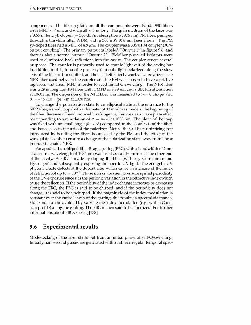
9.6. EXPERIMENTAL RESULTS 105
components. The fiber pigtails on all the components were Panda 980 fiberswith MFD ∼ 7 µm, and were all ∼ 1 m long. The gain medium of the laser wasa 0.65 m long yb-doped (∼ 300 dB/m absorption at 976 nm) PM fiber, pumpedthrough a thin-film filter WDM with a 300 mW 976 nm laser diode. The PMyb-doped fiber had a MFD of 4.8 µm. The coupler was a 30:70 PM coupler (30 %output coupling). The primary output is labeled ”Output 1” in figure 9.6, andthere is also a second output, ”Output 2”. PM-fiber pigtailed isolators wereused to eliminated back reflections into the cavity. The coupler serves severalpurposes. The coupler is primarily used to couple light out of the cavity, butin addition to this, it has the property that only light polarized along the slowaxis of the fiber is transmitted, and hence it effectively works as a polarizer. TheNPR fiber used between the coupler and the FM was chosen to have a relativehigh loss and small MFD in order to seed initial Q-switching. The NPR fiberwas a 29 m long non-PM fiber with a MFD of 3.33 µm and 9 dB/km attenuationat 1060 nm. The dispersion of the NPR fiber was measured to β2 = 0.046 ps2/m,β3 = -9.6 · 10−6 ps3/m at 1030 nm.
To change the polarization state to an elliptical state at the entrance to theNPR fiber, a small loop (with a diameter of 33 mm) was made at the beginning ofthe fiber. Because of bend induced birefringence, this creates a wave plate effectcorresponding to a retardation of ∆ = 3π/8 at 1030 nm. The plane of the loopwas fixed with an small angle (θ ∼ 5◦) compared to the slow axis of the fiber,and hence also to the axis of the polarizer. Notice that all linear birefringenceintroduced by bending the fibers is canceled by the FM, and the effect of thewave plate is only to ensure a change of the polarization state away from linearin order to enable NPR.
An apodized unchirped fiber Bragg grating (FBG) with a bandwidth of 2 nmat a central wavelength of 1034 nm was used as cavity mirror at the other endof the cavity. A FBG is made by doping the fiber (with e.g. Germanium andHydrogen) and subsequently exposing the fiber to UV light. The energetic UVphotons create defects at the dopant sites which cause an increase of the indexof refraction of up to∼ 10−3. Phase masks are used to ensure spatial periodicityof the UV-exposure since it is the periodic variation in the refractive index whichcause the reflection. If the periodicity of the index change increases or decreasesalong the FBG, the FBG is said to be chirped, and if the periodicity does notchange, it is said to be unchirped. If the magnitude of the index modulation isconstant over the entire length of the grating, this results in spectral sidebands.Sidebands can be avoided by varying the index modulation (e.g. with a Gaus-sian profile) along the grating. The FBG is then said to be apodized. For furtherinformations about FBGs see e.g [138].
9.6 Experimental results
Mode-locking of the laser starts out from an initial phase of self-Q-switching.Initially nanosecond pulses are generated with a rather irregular temporal spac-

106CHAPTER 9 - ENVIRONMENTALLY STABLE LOW REPETITION RATE
NONLINEAR POLARIZATION ROTATION BASED FIBER LASER
0
2
4
6
8
10
12
0 1000 2000 3000 4000
Pow
er /
a.u.
Time / µs
0 1 2 3
-0.5 0 0.5 1 1.5
Pow
er /
a.u.
Time / µs
-60
-50
-40
-30
-20
-10
0
2.4 2.6 2.8 3 3.2 3.4
Pow
er /
dB
Frequency / MHz
Figure 9.7: Left: Mode-locked startup from an initial Q-switched phase. Right:RF-spectrum of the mode-locked output around the fundamental frequency.The resolution BW was 1 kHz.
0
0.2
0.4
0.6
0.8
1
1.2
1015 1020 1025 1030 1035 1040 1045 1050
Pow
er /
a.u.
Wavelength / nm
Fit: τFWHM = 10.4 ps
Output 1Output 2
Grating
0
1
2
3
4
5
6
7
8
-60 -40 -20 0 20 40 60
SG
H. I
nten
sity
/ a.
u.
Delay / ps
τFWHM = 10.4 ps
0
2
4
-40 0 40Delay / ps
τFWHM =58 ps
Figure 9.8: Left: Output spectra from the laser. Dotted line: measured reflectiv-ity of the FBG. Right: Autocorrelation trace from the primary output, ”Output1”. (Insert: autocorrelation trace from ”Output 2”)
ing and amplitude, but as soon as mode-locking is initiated, Q-switching ceases.This method of mode-locking differs from the well known Q-switched mode-locking [65], where a mode-locked pulse train is generated underneath the en-velope of a Q-switched pulse. Figure 9.7 (left) shows the transition from Q-switched to mode-locked lasing. The mode-locked pulse train is not fully re-solved due to sampling. The insert of figure 9.7 (left) shows the mode-lockedpulse train on a shorter time scale. The repetition rate of the laser was 2.91 MHz.
Figure 9.8 (left) shows the output spectrum from the laser on a linear scale.The two outputs originate from the two arms of the 2x2 coupler, and the pri-mary output, ”Output 1” is the output which has the highest output power andshortest pulses. ”Output 2” comes from the NPR fiber side of the cavity, andsignificant spectral broadening can be observed there from propagation in theNPR fiber. The laser mode-locks at a launched pump power in the interval 180-300 mW. At a pump power of 300 mW, the primary output power was 8.9 mW,

9.6. EXPERIMENTAL RESULTS 107
and the ”Output 2” power was 0.8 mW. Both outputs were linearly polarizedalong the slow axis of the PM fiber pigtails. All data presented in this sectionwere measured at a pump power of 300 mW. Figure 9.8 (left) also shows themeasured reflectance from the FBG as a dotted line.
Figure 9.8 (right) shows the autocorrelation trace of the primary output. Theautocorrelation FWHM of the non-oscillating part was 10.4 ps correspondingto an average pulse duration of 8.3 ps (using a deconvolution factor of 1.25 asfound from the numerical calculations below (section 9.7)). The pulse stretchesconsiderably during one round trip. The insert of figure 9.8 (right) shows the au-tocorrelation trace of the secondary output from the laser. The autocorrelationFWHM was 58 ps corresponding to an average pulse duration of 43 ps (decon-volution factor of 1.36). The laser contains ∼ 34 m of fibers, and due to this longinteraction length between fiber and pulse, the total non-linear phase shift accu-mulated during one round trip is so large that the pulse cannot reproduce itselfevery round trip. As a consequence the laser output is noise-like mode-locked,with a few percent fluctuations from pulse to pulse. In figure 9.7 (right) the RFspectrum around the fundamental laser frequency can be seen. The RF spec-trum reveals a pedestal, which is typical for noise-like mode-locked lasers [139].The pedestal is 38 dB below the peak. The relative energy fluctuations of thepulses was calculated from the measured RF-spectrum to 25 % [139]. In spite ofnoise-like mode-locking, the long term stability of the laser was excellent. Thelong term stability was tested over a period of 200 hours, by monitoring the av-erage output power and no variation was observed. This was despite the fact,that the laser were simply freely lying in a cardboard box on a wooden tablein a room with no temperature control, and hence the stability is significantlybetter than that of the solid state lasers in our lab, which require optical tablesand stable temperatures.
9.6.1 Amplification and supercontinuum generation
To demonstrate the applicability of the laser, the primary output, ”Output 1”was amplified in a simple single-mode non-PM fiber amplifier, and subsequentlyused for supercontinuum generation in a nonlinear photonic crystal fiber (PCF).Figure 9.6 also shows the diagram of the amplifier and the PCF. The gain fiber ofthe amplifier was a 20 cm long non-PM highly yb-doped fiber (i.e. ∼ 1200 dB/mabsorption at 976 nm). The yb-doped fiber was pumped through a non-PM fiberpigtailed WDM with a 600 mW single-mode fiber pigtailed 974 nm laser diode.The fiber pigtails on the WDM were kept as short as possible (i.e. < 20 cm). Thenonlinear PCF (MFD ∼ 3.3 mum) was 11.4 m long and was simply spliced tothe amplifier (splice loss: ∼ 48 %). The other end of the PCF was angle cleavedin order to suppress back reflection into the amplifier. Figure 9.9 (left) showsthe output power from the amplifier vs. amplifier pump power before the PCFwas spliced on. The maximum output power was 410 mW corresponding to apulse energy of 141 nJ. Figure 9.9 (right) shows the amplified spectrum at threedifferent amplifier pump powers on a logarithmic scale, and only slight spectral

108CHAPTER 9 - ENVIRONMENTALLY STABLE LOW REPETITION RATE
NONLINEAR POLARIZATION ROTATION BASED FIBER LASER
0 50
100 150 200 250 300 350 400 450
0 100 200 300 400 500 600 700
Out
put p
ower
/ m
W
Pump power / mW
-70
-60
-50
-40
-30
-20
-10
0
10
1000 1020 1040 1060 1080 1100
Pow
er /
dB
Wavelength / nm
Fit: τFWHM = 10.4 ps Ppump = 0 mWPpump = 180 mWPpump = 600 mW
Figure 9.9: Left: Output power from the amplifier vs. amplifier pump power.Right: Amplified spectrum at three different amplifier pump powers.
0
1
2
3
4
5
6
7
8
-60 -40 -20 0 20 40 60
SG
H. I
nten
sity
/ a.
u.
Delay / ps
τFWHM = 11 ps
-60
-50
-40
-30
-20
-10
0
10
600 800 1000 1200 1400 1600 1800
Pow
er /
dB
Wavelength / nm
Figure 9.10: Left: Autocorrelation after maximum amplification of the primaryoutput. The autocorrelation FWHM of the non-oscillating part is 11 ps corre-sponding to a pulse duration of 7.8 ps. Right: Supercontinuum generated afterpulse propagation through a photonic crystal fiber.
broadening was observed.Figure 9.10 (left) shows the measured autocorrelation trace after amplifica-
tion. The pulse duration only increased slightly during amplification, and theautocorrelation FWHM of the non-oscillating part was 11.0 ps at maximum am-plification corresponding to an average pulse duration of 8.8 ps. At maximumamplification the output power through the PCF was 213 mW. Figure 9.10 (right)shows the supercontinuum (SC) generated after pulse propagation through thePCF. The SC spans from 600 nm to 1750 nm. The noise from the laser also leadsto noise in the SC, but averaging times of < 1 s were found to be sufficientfor stable noise-free averaged spectra. For most linear applications of the SC(e.g. transmission measurements etc.) such averaging times are sufficientlyshort. The SC is generated through multi soliton generation and this form ofSC generation is also associated with pulse to pulse fluctuations even if the in-put is more stable. In spite of the low average power of the SC compared to

9.7. NUMERICAL MODEL AND SIMULATIONS 109
the SC demonstrated in chapter 8, the SC source presented here is expected tobe highly applicable in many fields, as it is based on a fully-spliced environ-mentally stable fiber laser system, based on readily available single-mode fibercomponents. Compared to other fiber laser sources, it is the low repetition ratefrom this laser that enables SC generation at the power levels obtainable afteramplification with the use of standard single-mode fiber pigtailed laser diodes.SC generation can also be obtained at higher repetition rates if shorter femto-second pulses are used. However this requires more complicated amplificationschemes with subsequent pulse compression before launching the pulse into thePCF. Alternatively pulse-picking can also be used.
9.7 Numerical model and simulations
An important component of the presented laser is the FBG. Besides working asa mirror, the FBG is also the primary source of pulse shaping, which is needed toobtain short pulses from the laser. Without this form of pulse shaping (i.e. if theFBG is replaced by a broadband mirror), much longer pulses (i.e. > 100-1000 ps)would be obtained from the laser. When working in the noise-like mode-lockedregime, it is possible to use strong spectral filtration to attain temporal com-pression inside the cavity. As all the fibers in the cavity have high normal dis-persion, and as no means of introducing anomalous dispersion are used, thepulses circulating inside the cavity are highly chirped. As a consequence, tem-poral compression can be obtained by spectral filtration. A numerical modelof the laser was developed to further investigate the difference between tempo-ral compression by spectral filtration and temporal compression by dispersioncompensation, and to investigate dependence of different parameters.
The model is based on the operator algebra introduced in section 9.2 and onsolving the NLSE in each fiber segment in succession. The laser is divided intothree fiber segments: 0.65 m PM gain fiber and 4 m passive PM fiber between theFBG and the coupler, and 30 m nonlinear non-PM fiber between the coupler andthe FM. NPR in between the coupler and the FM is handled in a similar way as inthe calculations in section 9.2, except that the effect of the NPR operator, OCP
NPR,is replaced by an integration of the NLSE for two coupled slowly varying fieldsin the CP representation (equations 2.28 and 2.29). The last two fiber segmentsare modeled by the standard NLSE for a single linear polarization state (equa-tion 2.18). As no SRS was present in the output from the experimental laser, itis reasonable to neglect the Raman terms in the NLSE. Measured losses at inter-sections between different components are also included. The gain medium wasmodeled with an unsaturated peak gain coefficient of 25 dB/m and a Gaussianspectral gain profile with a bandwidth of 40 nm (FWHM). A coupling betweenlight propagating in both directions through the gain medium was includedthrough the gain average power saturation. The FBG was modeled by a super

110CHAPTER 9 - ENVIRONMENTALLY STABLE LOW REPETITION RATE
NONLINEAR POLARIZATION ROTATION BASED FIBER LASER
Fiber type: Gain Passive NPRLength / m: 0.65 4 30β2 / ps2/m: 0.023 0.023 0.046β3 / ps3/m: 3.9 · 10−5 3.9 · 10−5 -9.6 · 10−6
γ / (m W)−1: 6.7·10−3 3.6·10−3 14·10−3
α / m−1: 0 0 2.07·10−3
Table 9.1: Coefficients for the three different fibers used in the model of the laser.
Gaussian function to match the measured reflectivity of the FBG:
A(ω)→ A(ω) · exp(
− 22·5 ln(2)( ω
ωFWMN
)2·5)
,
where the FWHM bandwidth, ωFWMN, corresponds to a bandwidth of 2.0 nm.The other relevant coefficients used in the NLSE to model the three fibers can beseen in table 9.1.
Because of the strong pulse shaping from the strong spectral filtration, thesimulations quickly converge from a long noise pulse to a regime where themonitored parameters fluctuate around stable values. No dependency was foundon the choice of input pulse (non-noise pulses were also tested). Furthermore,dependency on the numerical resolution was also tested, and the number of datapoints was chosen sufficiently large to eliminate any dependence on the numeri-cal resolution. At a saturation average power of Psat = 40 mW, the calculated av-erage output powers from the simulation matched the output powers from theexperimental laser. Although the model is simplified compared to the real laser,and for instance does not include the unknown bend induced birefringence ofthe long NPR fiber, it does reproduce the experimental data qualitatively, andin agreement with the theory, the reflection, | ~ALP
out|2/| ~ALPin |2, from NPR section
tends to zero, as the input peak power is decreased. The pulse experiences bothspectral and temporal broadening throughout the entire cavity and is only com-pressed (both spectrally and temporally) at the FBG. Figure 9.11 (left) shows thecalculated averaged output spectra corresponding the the ”Output 1” and ”Out-put 2” spectra from the experimental laser. The spectra were averaged over 1000round trips after the noise-like mode-locked regime was reached.
Figure 9.11 (right) shows the averaged output pulse temporal shapes, andfigure 9.12 shows the averaged autocorrelation traces. The ”Output 1” aver-aged pulse duration was 10.4 ps and the ”Output 2” averaged pulse durationwas 58 ps. The autocorrelation FWHM of the non-oscillating parts were 13.0 psand 79 ps respectively, and hence the deconvolution factors between the auto-correlation FWHM and the averaged pulse duration FWHM for the two out-puts are 1.25 and 1.36 respectively. Before calculating the averaged output pulsetemporal shape, the midpoint of the temporal window was moved to the meanpeak of the pulse. If this is not done, a spreading of the averaged pulse tem-porals shape would be observed due to drifting pulse position in the temporal

9.7. NUMERICAL MODEL AND SIMULATIONS 111
0 0.1 0.2 0.3 0.4 0.5 0.6 0.7 0.8 0.9
1
1010 1020 1030 1040 1050 1060
Pow
er /
a.u.
Wavelength / nm
Output 1Output 2
0 0.1 0.2 0.3 0.4 0.5 0.6 0.7 0.8 0.9
1
-100 -50 0 50 100 150
Pow
er /
a.u.
Time / ps
Output 1Output 2
Figure 9.11: Left: Calculated averaged output spectra at output powers corre-sponding to the experimentally measured values. Right: Calculated averagedoutput temporal shapes.
0
1
2
3
4
5
6
7
8
-60 -40 -20 0 20 40 60
SG
H In
tens
ity /
a.u.
Delay / ps
0
1
2
3
4
5
6
7
8
-150 -100 -50 0 50 100 150
SG
H In
tens
ity /
a.u.
Delay / ps
Figure 9.12: Calculated averaged autocorrelation trace of ”Output 1” at outputpowers corresponding to the experimentally measured values. The autocorrela-tion FWHM of the non-oscillating part is 13.0 ps. Right: Calculated autocorrela-tion trace of ”Output 2”. The autocorrelation FWHM is 79.0 ps.
window. The averaged temporal pulse shape may, however, still be deceiving,as the pulse changes shape due to noise fluctuations. In the calculation of the av-eraged autocorrelation trace, the individual autocorrelation traces are howeverintrinsically centered due to the definition of the autocorrelation function, andhence the calculated averaged autocorrelation function gives a better picture ofthe true average pulse duration then the directly averaged temporal shape.
A significant temporal compression is observed in agreement with the ex-perimentally measured pulse durations. To further investigate the importanceof the FBG on the output pulse duration, a series of simulations were performedwhere the bandwidth of the FBG was varied while keeping all other parametersfixed. Figure 9.13 (left) shows the calculated ”Output 1” autocorrelation FWHMvs. the FWHM bandwidth of the FBG. Short pulses directly out of the oscillatorare a key issue for nonlinear applications, as the laser is noise-like mode-locked,
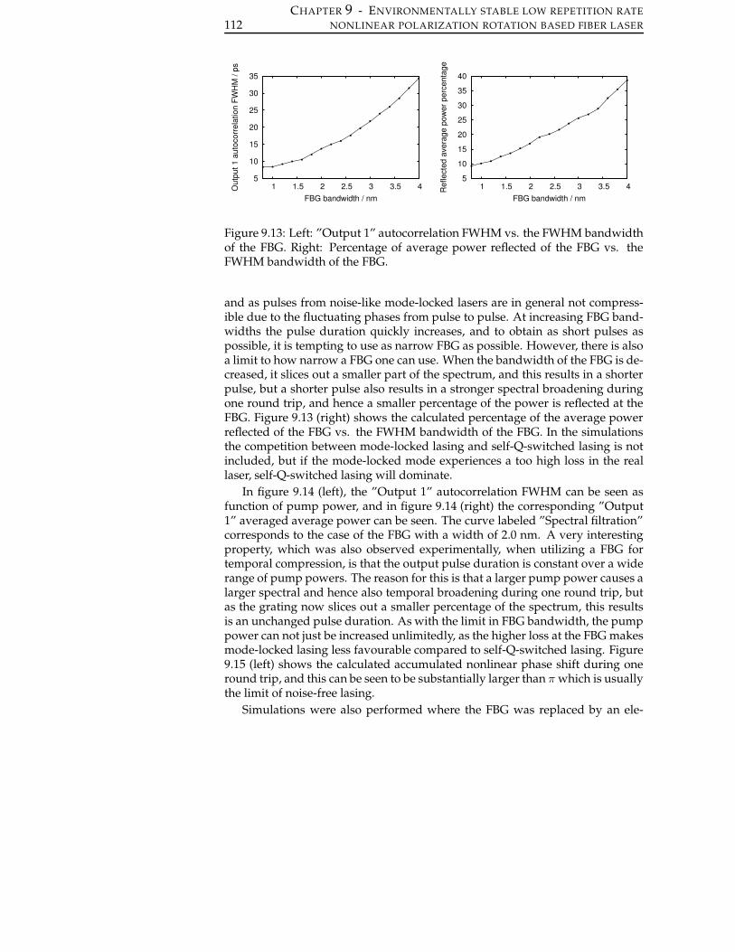
112CHAPTER 9 - ENVIRONMENTALLY STABLE LOW REPETITION RATE
NONLINEAR POLARIZATION ROTATION BASED FIBER LASER
5
10
15
20
25
30
35
1 1.5 2 2.5 3 3.5 4Out
put 1
aut
ocor
rela
tion
FWH
M /
ps
FBG bandwidth / nm
5
10
15
20
25
30
35
40
1 1.5 2 2.5 3 3.5 4Ref
lect
ed a
vera
ge p
ower
per
cent
age
FBG bandwidth / nm
Figure 9.13: Left: ”Output 1” autocorrelation FWHM vs. the FWHM bandwidthof the FBG. Right: Percentage of average power reflected of the FBG vs. theFWHM bandwidth of the FBG.
and as pulses from noise-like mode-locked lasers are in general not compress-ible due to the fluctuating phases from pulse to pulse. At increasing FBG band-widths the pulse duration quickly increases, and to obtain as short pulses aspossible, it is tempting to use as narrow FBG as possible. However, there is alsoa limit to how narrow a FBG one can use. When the bandwidth of the FBG is de-creased, it slices out a smaller part of the spectrum, and this results in a shorterpulse, but a shorter pulse also results in a stronger spectral broadening duringone round trip, and hence a smaller percentage of the power is reflected at theFBG. Figure 9.13 (right) shows the calculated percentage of the average powerreflected of the FBG vs. the FWHM bandwidth of the FBG. In the simulationsthe competition between mode-locked lasing and self-Q-switched lasing is notincluded, but if the mode-locked mode experiences a too high loss in the reallaser, self-Q-switched lasing will dominate.
In figure 9.14 (left), the ”Output 1” autocorrelation FWHM can be seen asfunction of pump power, and in figure 9.14 (right) the corresponding ”Output1” averaged average power can be seen. The curve labeled ”Spectral filtration”corresponds to the case of the FBG with a width of 2.0 nm. A very interestingproperty, which was also observed experimentally, when utilizing a FBG fortemporal compression, is that the output pulse duration is constant over a widerange of pump powers. The reason for this is that a larger pump power causes alarger spectral and hence also temporal broadening during one round trip, butas the grating now slices out a smaller percentage of the spectrum, this resultsis an unchanged pulse duration. As with the limit in FBG bandwidth, the pumppower can not just be increased unlimitedly, as the higher loss at the FBG makesmode-locked lasing less favourable compared to self-Q-switched lasing. Figure9.15 (left) shows the calculated accumulated nonlinear phase shift during oneround trip, and this can be seen to be substantially larger than π which is usuallythe limit of noise-free lasing.
Simulations were also performed where the FBG was replaced by an ele-
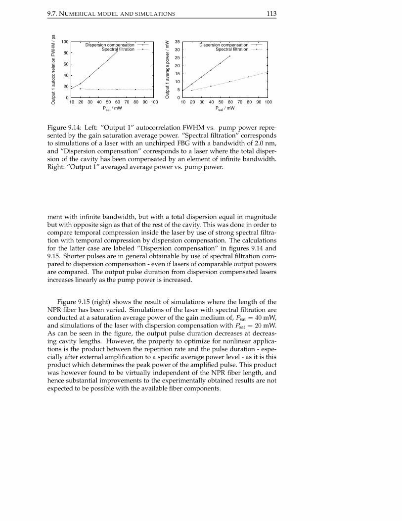
9.7. NUMERICAL MODEL AND SIMULATIONS 113
0
20
40
60
80
100
10 20 30 40 50 60 70 80 90 100Out
put 1
aut
ocor
rela
tion
FWH
M /
ps
Psat / mW
Dispersion compensationSpectral filtration
0
5
10
15
20
25
30
35
10 20 30 40 50 60 70 80 90 100
Out
put 1
ave
rage
pow
er /
mW
Psat / mW
Dispersion compensationSpectral filtration
Figure 9.14: Left: ”Output 1” autocorrelation FWHM vs. pump power repre-sented by the gain saturation average power. ”Spectral filtration” correspondsto simulations of a laser with an unchirped FBG with a bandwidth of 2.0 nm,and ”Dispersion compensation” corresponds to a laser where the total disper-sion of the cavity has been compensated by an element of infinite bandwidth.Right: ”Output 1” averaged average power vs. pump power.
ment with infinite bandwidth, but with a total dispersion equal in magnitudebut with opposite sign as that of the rest of the cavity. This was done in order tocompare temporal compression inside the laser by use of strong spectral filtra-tion with temporal compression by dispersion compensation. The calculationsfor the latter case are labeled ”Dispersion compensation” in figures 9.14 and9.15. Shorter pulses are in general obtainable by use of spectral filtration com-pared to dispersion compensation - even if lasers of comparable output powersare compared. The output pulse duration from dispersion compensated lasersincreases linearly as the pump power is increased.
Figure 9.15 (right) shows the result of simulations where the length of theNPR fiber has been varied. Simulations of the laser with spectral filtration areconducted at a saturation average power of the gain medium of, Psat = 40 mW,and simulations of the laser with dispersion compensation with Psat = 20 mW.As can be seen in the figure, the output pulse duration decreases at decreas-ing cavity lengths. However, the property to optimize for nonlinear applica-tions is the product between the repetition rate and the pulse duration - espe-cially after external amplification to a specific average power level - as it is thisproduct which determines the peak power of the amplified pulse. This productwas however found to be virtually independent of the NPR fiber length, andhence substantial improvements to the experimentally obtained results are notexpected to be possible with the available fiber components.

114CHAPTER 9 - ENVIRONMENTALLY STABLE LOW REPETITION RATE
NONLINEAR POLARIZATION ROTATION BASED FIBER LASER
40
60
80
100
120
140
10 20 30 40 50 60 70 80 90 100
φ NL
Psat / mW
Dispersion compensationSpectral filtration
10
15
20
25
30
35
40
20 25 30 35 40
Out
put 1
aut
ocor
rela
tion
FWH
M /
ps
NPR fiber length / m
Dispersion compensationSpectral filtration
Figure 9.15: Left: Calculated nonlinear phase vs. pump power represented bythe gain saturation average power. ”Spectral filtration” corresponds to sim-ulations of a laser with an unchirped FBG with a bandwidth of 2.0 nm, and”Dispersion compensation” corresponds to a laser where the total dispersion ofthe cavity have been compensated by an element of infinite bandwidth. Right:”Output 1” autocorrelation FWHM vs. NPR fiber length.
9.8 Intra cavity Raman continuum generation
To illustrate the limitations on the obtainable repetition rate set by Raman scat-tering, results of a second experimental implementation of the laser are pre-sented here. Figure 9.16 shows a diagram of the laser.
Coupler
HRc)
6m PM 265m fiberTR
PM WDM
Yb−fiber
Laser diode IsolatorPM
PM 20:80
Output 2Output1
PMIsolator
50m PM−fiber
FM
Figure 9.16: Diagrams of an experimental implemented laser with a repetitionrate of 360 kHz. In this laser the NPR fiber was a 265 m non-PM fiber, and thelength of the ytterbium doped fiber was 6 m. The FBG was replaced by a grat-ing compressor. (HR: High Reflector, TR: Transmission Gratings, FM: FaradayMirror).
In this laser the NPR fiber was a 265 m non-PM fiber with the same fibercharacteristics as in the previous laser (figure 9.3). The length of the ytterbiumdoped fiber was increased to 6 m (but otherwise also with the same characteris-tics as before) in order to effectively move the gain band of the ytterbium fiber tohigher wavelengths. This is possible as the last (unpumped) section of the ytter-bium fiber exhibits a wavelength dependent absorption with higher absorptionat lower wavelengths. When a long piece of ytterbium fiber is used, the 976 nm

9.8. INTRA CAVITY RAMAN CONTINUUM GENERATION 115
isolator can be omitted. As a result of the longer yb-doped fiber, an extra lengthof 50 m PM fiber was needed on the ”Output 1” side in order to have sufficientSBS and RB backscattering to start the laser. The FBG was in this laser replacedby a grating compressor. The double pass dispersion of the grating compressorwas -2.7 ps2, and hence only a partial dispersion compensation (∆β2 = 22.1 ps2)was obtained with this approach.
-60-55-50-45-40-35-30-25-20-15-10
1000 1050 1100 1150 1200 1250
Pow
er /
dB
Wavelength / nm
Output 1Output 2
Figure 9.17: Output 1 and Output 2 spectra from the 360 kHz laser.
The repetition rate of this laser was 360 kHz, but the pulse duration wasalso long (i.e. > 100 ps). The output spectra from the laser at a pump powerof 300 mW can be seen in figure 9.17. The repetition rate and the obtainableoutput pulse duration was found to be limited by the onset of SRS, and in the”Output 2” spectrum coming from the NPR side of the cavity, the first threestokes pulses are clearly visible. The stokes pulses are generated inside the cav-ity, and hence correspond to a substantial loss to the mode-locked pulse. SRSis a nonlinear loss mechanism affecting only a pulse and not a low power cwmode, but because of the high modulation depth of the NPR fiber section, sin-gle pulse (noise-like) mode-locking was possible with this laser configuration.Due to the low repetition rate, this peak power was sufficient to generate a Ra-man spectrum with a width of 190 nm. Only the spectral part overlapping withthe bandwidth of the gain medium and the grating compressor was amplified,and the rest simply filtered out every round trip, as can be seen from the ”Out-put 1” spectrum. Hence the output only contained the fundamental pulse. Eventhough longer fiber lengths were also experimentally investigated, the 360 kHzrepetition rate constitutes the experimentally found limit in single pulse (noise-like) mode-locking. At longer fiber lengths or at smaller net cavity dispersionthe laser jumped into a multi pulse mode where two or more noise-like pulseswere simultaneously present inside the cavity.
Although many different cavity configurations were experimentally investi-gated (i.e. different cavity lengths, different fiber types, different compressionmechanisms and settings, etc.), short (i.e. sub 10 ps) pulses were only obtained

116CHAPTER 9 - ENVIRONMENTALLY STABLE LOW REPETITION RATE
NONLINEAR POLARIZATION ROTATION BASED FIBER LASER
at higher repetition rates, as in the laser presented in section 9.5. The primarylimitation to the output pulse duration is believed not to be set by SRS, butrather by the nature of noise-like pulse evolution inside long sections of fiber.Pulse durations in the 100 ps range are not really interesting, as shorter pulsesare obtainable from fast laser diodes. The approach of using a long piece ofyb-doped fiber to avoid the use of the 980 nm isolator was also found to beinadequate to obtain shortest possible pulses.
9.9 All-polarization maintaining fiber laser
Although the FM intrinsically compensates the linear polarization evolution in-side the non-PM NPR fiber, and hence stabilizes NPR, NPR in non-PM fibersis still a function of the linear polarization state, and hence also of the linearpolarization evolution inside the fiber. As a consequence, the laser outputs fromthe above mentioned lasers are susceptible to strong perturbations to the non-PM fiber. Although the laser is still much more stable compared to fiber lasersutilizing NPR in a fiber where the linear polarization evolution has not beencompensated by a FM, it would be better if the total NPR could be made inde-pendent of the linear birefringence altogether. It was both experimentally andtheoretically demonstrated in reference [140] that NPR, to a good approxima-tion, is independent of the linear birefringence in highly birefringent fibers witha linear beat length much shorter then the nonlinear beat length.
A FM still has to be used to avoid problems with environmentally inducedchanges of the linear polarization evolution, but if the non-PM fiber in betweenthe FM and the coupler is replaced by a PM fiber in which NPR can occur, thelaser can be made environmentally stable even against strong perturbations ofthe fibers. When neglecting losses, dispersion and walk-off due to the groupbirefringence, NPR in a PM fiber is described by [1]:
∂
∂zAx(t) = +iγ(|Ax(t)|2 +
2
3|Ay(t)|2)Ax(t) +
i
3Ax(t)∗Ay(t)2 exp(−2i∆β0z)
∂
∂zAy(t) = +iγ{(|Ay(t)|2 +
2
3|Ax(t)|2)Ay(t) +
i
3Ay(t)∗Ax(t)2 exp(2i∆β0z).
(9.1)
For NPR to occur, the polarization state must not be linearly polarized alongone of the two birefringent axes, x and y. However, as the polarization statequickly evolves into elliptically polarized light at other input polarization di-rections, it is sufficient to launch linearly polarized light into the fiber with anangle between the polarization axis and the birefringent axes. This can easily beimplemented experimentally in an all-fiber solution, by splicing two PM fiberstogether with an angle between the axes of the two fibers. Figure 9.18 showsthe calculated reflection through a polarizer after NPR in a 30 m long PM fiberand reflection off a FM. The NPR fiber was modeled with nonlinear coefficient,γ = 9.2 · 10−3 (m W)−1 and phase birefringence, ∆n = 10−4, corresponding

9.9. ALL-POLARIZATION MAINTAINING FIBER LASER 117
0
20
40
60
80
100
0 5 10 15 20 25
Ref
lect
ion
/ %
Normalized peak power / P / (γL)-1
θ = 10o
θ = 20o
θ = 30o
θ = 40o
Figure 9.18: Calculated reflection through a polarizer after NPR in a PM fiber(parameters in the text). Reflection is calculated for different angles betweenthe polarizer and the birefringent axis of the fiber on the input side, and at theother end the light is reflected at a FM. Solid and dashed lines represent calcu-lations using equations 9.1, and filled circles represent calculations where theexp(±2i∆β0z) terms in equations 9.1 have been neglected.
to ∆β0 = 610 m−1 (values are chosen to match the PM fiber used in the ex-periments below (section 9.9.1). The reflection is calculated using equations 9.1(solid and dashed lines) for different angles, θ, between the polarizer and theaxis of the PM fiber.
Again the reflection initially increases from zero with increasing peak power.The highest reflection is obtained at angles closest to θ = 45◦, but also requires ahigher peak power. Compared to figure 9.2, higher peak powers correspondingto higher nonlinear phase shifts are also required to obtain maximum reflectiv-ity.
As the exp(±2i∆β0z) terms in equations 9.1 are very fast oscillating func-tions of z and hence on average effectively do not contribute to the NPR, theycan to a very good approximation be neglected. The filled circles in figure 9.18represent calculations were the exp(±2i∆β0z) in equations 9.1 have been ne-glected, and as can be seen, the results are indistinguishable from the calcula-tions where the exp(±2i∆β0z) terms were not neglected. This approximation isthe high-birefringence approximation of the NLSE leading to equations 2.30 and2.31. As the environmentally induced changes to the birefringence of the fiber iscontained in ∆β0(z), the NPR is hence independent of environmentally inducedchanges to the birefringence when the exp(±2i∆β0z) terms in equations 9.1 arenegligible.

118CHAPTER 9 - ENVIRONMENTALLY STABLE LOW REPETITION RATE
NONLINEAR POLARIZATION ROTATION BASED FIBER LASER
PM 30:70Coupler
11m PM−fiber
Angled splice
0.65m PM Yb−fiber
FBG FMPM WDM
Output 2
Isolator976nm
Laser diode976nm300mW
IsolatorPM
IsolatorPM
Output 1
Figure 9.19: Diagram of the all-PM laser configuration.
9.9.1 Experimental setup and results
All-PM versions of the proposed laser configuration with NPR in a PM fiberhave also been investigated experimentally. For the experiments a PM fiber witha MFD of 4.11 µm, and an attenuation of 8 dB/km at 1060 nm was used. Thegroup birefringence of the fiber was measured to: ng ∼ 0.35 · 10−4 at 1030 nm.This corresponds to a group velocity mismatch of 117 fs/m. The dispersionof the PM fiber was measured to β2 = 0.024 ps2/m, β3 = 10.2 · 10−6 ps3/m at1030 nm. Short pulses (i.e. sub 10 ps) were only obtained at higher repetitionrates compared to the version with NPR in a non-PM fiber. Here results from an5.96 MHz version of an all-PM laser is presented. Figure 9.19 shows a diagram ofthe laser configuration. The laser was identical to the laser shown in figure 9.6,except that the 29 m long non-PM NPR fiber was replaced with an 11 m longPM fiber.
At an angle of θ ∼ 30◦ between the slow axis of the coupler (polarizer) andthe slow axis of the PM fiber, and at a pump power of 300 mW, self-startingnoise-like mode-locking was obtained. The pump power could be turned backdown to ∼ 150 mW before mode-locking ceased. The repetition rate of the laserwas 5.96 MHz, and the ”Output 1” and ”Output 2” powers were 8.0 mW and0.50 mW respectively. Figure 9.20 (left) shows the output spectra from the laserat a pump power of 300 mW on a linear scale (Insert: logarithmic scale). TheFWHM spectral width was 1.17 nm and 1.87 nm of ”Output 1” and ”Output 2”respectively.
Figure 9.20 (right) shows the measured autocorrelation trace. The FWHM ofthe non-oscillating part of the autocorrelation trace was 7.0 ps, correspondingto an average pulse duration of 5.6 ps (deconvolution factor 1.25). The RF spec-trum around the fundamental laser frequency can be seen in figure 9.21 (left).The pedestal was 38 dB below the peak. The calculated relative energy fluctu-ations were 6.1 %, and hence less than the relative energy fluctuations from the2.91 MHz laser with NPR in a non-PM fiber. The stability of the laser was alsoexcellent, and the fibers (even the NPR fiber) could be moved around and bendstrongly without any detectable change to the output power, pulse spectra orautocorrelation trace. The long term stability of the laser was also tested over

9.9. ALL-POLARIZATION MAINTAINING FIBER LASER 119
0
0.2
0.4
0.6
0.8
1
1.2
1025 1030 1035 1040 1045 1050
Pow
er /
a.u.
Wavelength / nm
Output 1Output 2
-60
-30
0
1010 1030 1050
Pow
er /
dB
Wavelength / nm
0
1
2
3
4
5
6
7
8
-40 -30 -20 -10 0 10 20 30 40
SG
H. I
nten
sity
/ a.
u.
Delay / ps
τFWHM = 7.0 ps
Figure 9.20: Left: Output spectrum from the all-PM laser at a pump power of300 mW. Insert: logarithmic scale. Right: Autocorrelation trace of the ”Output1” pulse. The autocorrelation FWHM of the non-oscillating part was 7.0 ps.
a period of 200 hours. Figure 9.21 (right) shows the measured output powerfrom the laser. The output power was measured with a setup with a very fastintegration time, so that variations in the average output power due to pulseto pulse fluctuations can be seen. The standard deviation was 0.25 mW, andno long time variations in the average output power was observed. In spite ofthe quite large variations in the output power, the average value does hence notchange on a long time scale. The insert of figure 9.21 (right) shows the measuredoutput power over a time period of 2 s and with a sampling rate of 1 kHz. Ascan be seen, the fluctuations are very rapid, and can be easily averaged out overaveraging times of ∼ 1 s.
-60
-50
-40
-30
-20
-10
0
3 4 5 6 7 8 9
Pow
er /
dB
Frequency / MHz
0
2
4
6
8
10
0 50 100 150 200
Out
put 1
pow
er /
mW
Time / h
6 7 8 9
10
0 0.5 1 1.5 2
Pow
er /
mW
Time / s
Figure 9.21: Left: RF-spectrum of the mode-locked output around the funda-mental frequency at a pump power of 300 mW. The resolution BW was 1 kHz.Right: Long term output power stability measurement of the all-PM laser. Themeasurement shows quite large pulse to pulse fluctuations but a stable averagepower level. Insert: Output power on a short time scale measured with sam-pling rate of 1 kHz.

120CHAPTER 9 - ENVIRONMENTALLY STABLE LOW REPETITION RATE
NONLINEAR POLARIZATION ROTATION BASED FIBER LASER
9.10 Summary
In summary, a new mode-locked laser configuration has been investigated the-oretically and experimentally. The mode-locking mechanism is based on NPR,and environmentally stable low-repetition rate laser outputs are possible formlasers with no sections of free space optics. The mode-locked state is noise-likewith pulse to pulse fluctuations. However, as there are no long term fluctu-ations, the outputs can easily be averaged. An alternative approach of usingstrong spectral filtration instead of dispersion compensation for intra cavitypulse shaping was investigated theoretically and experimentally. This approachresulted in the shortest pulses obtained from the proposed laser configuration.Highest environmental stability was obtained form an all-PM laser with NPRin a PM fiber. The laser is further demonstrated to be stable towards self-Q-switching of the gain medium (and in fact uses this mechanism to start-up), andoptically fragile components like SESAMs and pump lasers can be omitted orisolated. As an application of the proposed laser configuration 213 mW of su-percontinuum (600 nm to 1750 nm) was demonstrated form an fiber laser systemwith no sections of free-space optics.
9.11 Outlook
The proposed laser configuration with NPR between a FM and a polarizer is in-teresting as it is implementable as an all-fiber environmentally stable fiber laser.The combination of a FM and a polarizer, however, does not allow for noise-freemode-locking, as high feedbacks are only possible at nonlinear phase shifts be-yond the noise-free limit. For applications where short term averaging is not aproblem, but where the long term stability is important, this type of laser con-figuration may be a good solution. Furthermore, short (i.e. sub 10 ps) singlepulsed lasing is possible from this type of configuration at repetition rates in the1-6 MHz range, and this range is interesting for fast material processing. Lowrepetition rates are however also obtainable through pulse picking of noise-freelasers, but this requires more complicated and expensive setups, the proposedlaser configuration may hence be a cheaper alternative for some applications. Itis however believed, that the laser is best suited as a stable source for simple SCgeneration.
121
CHAPTER 10
Summary and perspectives
The focus of this thesis has been the development of new mode-locked fiberlasers and fiber laser systems. The recent development of photonic crystal fibers(PCF) has provided new fiber based products which are highly interesting forthe development of such systems. The flexibility and design freedoms of PCFsenable interesting new possibilities compared to standard fibers. A main part ofthis work has been devoted to the investigation of different applications of suchPCFs, and how they can contribute to the development of mode-locked fiberlaser systems.
A primary requirement for the generation of femtosecond pulses from fiberlaser systems operating near 1 µm and with no sections of free space optics,is the availability of fiber based components with anomalous dispersion. Inchapter 5 a fiber laser based on a solid-core photonic bandgap (SC-PBG) fiberfor intra cavity dispersion compensation was demonstrated. SC-PBG fibers arehighly integrable with standard fibers and can be spliced to these without in-troducing Fresnel reflections. The pulse duration was found to be limited bythe high third order dispersion of the SC-PBG fiber. However, a pulse dura-tion comparable to pulse durations obtainable from other fiber lasers with fiberbased dispersion compensation was demonstrated. 158 fs pulses were obtainedafter external compression in a hollow core photonic bandgap (HC-PBG) fiber.HC-PBG fibers enables fiber based outputs and external compression withouthigh nonlinear induced pulse distortions.
An alternative to the use of linear dispersive elements for intra cavity disper-sion compensation was investigated in chapter 8. After external compression,800 fs pulse durations were obtained form a fiber laser based on temporal com-

122 CHAPTER 10 - SUMMARY AND PERSPECTIVES
pression in a high modulation depth SESAM. More importantly, the laser wasused for high average power blue-extended supercontinuum generation in asmall core PCF after amplification in a setup with no dispersion compensationelements.
Within recent years, fiber laser systems have become a serious alternativeto the classical solid-state laser systems. A major reason for this developmentis the development of high efficiency ytterbium based fiber amplifiers, whichcombined with high power laser diodes enables average power amplificationeven to the kW level. Ytterbium doped amplifiers with output power levels of10-100 W combined with a mode-locked fiber laser seed source, provides com-petitive alternatives to other amplified mode-locked fiber laser systems. An im-portant property of such systems is the stability towards changing conditions inthe surrounding environment. Such changes can affect the output from mode-locked fiber lasers and the polarization evolution in amplifiers with the resultof decreased throughput and pulse quality after final compression in gratingcompressors. In chapter 6, an environmentally stable mode-locked fiber laserwas presented, and in chapter 7 amplification of this oscillator to the micro-Joule level was demonstrated in an environmentally stable setup. The setupwas based on a single mode polarization maintaining (PM) standard fiber oscil-lator and a large core single mode double clad PM PCF amplifier.
A primary limitation to the generation of high pulse peak powers from fiberbased systems is the high nonlinear phase shift accumulated by a pulse dueto tight confinement and long interaction lengths in fibers. To reach the highestpulse energies without high pulse distortions in chapter 7, advantage of the spe-cial pulse output shape from the oscillator was taken, and this enabled nonlinearphase shifts above the nonlinear limit. The oscillator operated in the self-similarregime, and hence generated parabolic like pulses. Direct amplification of para-bolic pulses was further investigated theoretically in chapter 7, and comparedto self-similar amplifiers, this approach was found to have a higher theoreticallimit of the obtainable pulse energy.
To utilize the full potential of fibers in fiber lasers, experimental implementa-tions should be realized with no sections of free space optics. Prior to this work,intrinsically environmentally stable mode-locked fiber lasers with no sectionsof free space optics have only been demonstrated with the use of PM fibers andwith a SESAM as the mode-locking mechanism. In chapter 9, an intrinsicallyenvironmentally stable mode-locked fiber laser with no sections of free spaceoptics and based on nonlinear polarization rotation was demonstrated. As anapplication, super continuum generation from a stable source with no sectionsof free space optics was proposed and demonstrated.
The further development of fiber laser systems is also in the future expectedto depend highly on the continued development of PCFs. Especially the devel-opment of double clad PCFs with larger cores will push the obtainable pulseenergies and peak powers even further. On the integrability side, there is alsoa lot of work to be done in obtaining amplification to the highest power levelswithout sections of free space optics. As fiber laser systems with higher stability

123
are developed, the number of applications will also continue to increase, andin the future, mode-locked fiber lasers will perhaps find applications on muchbroader commercial markets. In the near future, it is likely that the realizationof commercial high average power supercontinuum sources will have a highimpact on areas such as e.g. microscopy and spectroscopy in fields of medicine,biology and chemistry, and hence bring applications of mode-locked fiber laserout of the optical laboratories.


125
Bibliography
[1] G. P. Agrawal. Nonlinear Fiber Optics. Academic Press, San Diego, CA.(1995).
[2] C. L. Thomsen, D. Madsen, S. R. Keiding, J. Thøgersen, and O. Chris-tiansen. “Two-photon dissociation and ionization of liquid water studiedby femtosecond transient absorption spectroscopy”. J. Chem. Phys., 110,no. 7, pp. 3453–3462 (1999).
[3] T. Udem, R. Holzwarth, and T. W. Hansch. “Optical frequency metrol-ogy”. Nature, 416, pp. 233–237 (2002).
[4] P. U. Jepsen, R. H. Jacobsen, and S. R. Keiding. “Generation and detectionof terahertz pulses from biased semiconductor antennas”. J. Opt. Soc. Am.B, 13, no. 11, pp. 2424–2436 (1996).
[5] H. N. Paulsen, K. M. Hilligsøe, J. Thøgersen, S. R. Keiding, and J. J. Larsen.“Coherent anti-Stokes Raman scattering microscopy with a photonic crys-tal fiber based light source”. Opt. Lett., 28, no. 13, pp. 1123–1125 (2003).
[6] I. Hartl, X. D. Li, C. Chudoba, R. K. Ghanta, T. H. Ko, J. G. Fujimoto,J. K. Ranka, and R. S. Windeler. “Ultrahigh resolution optical coherencetomography using continuum generation in a air-silica microstructure op-tical fiber”. Opt. Lett., 26, no. 9, pp. 608–610 (2001).
[7] P. Weigl, A. Kasenbacher, and K. Werelius. “Dental applications”. Top.App. Phys., 96, pp. 167–185 (2004).
[8] A. Tunnermann, J. Limpert, and S. Nolte. “Ultrashort pulse fiber lasersand amplifiers”. Top. App. Phys., 96, pp. 35–53 (2004).
[9] D. Breitling, C. Fohl, F. Dausinger, T. Kononenko, and V. Konov. “Drillingof metals”. Top. App. Phys., 96, pp. 131–154 (2004).
[10] H. A. Haus. “Mode-Locking of Lasers”. IEEE J. Selected Top. in QuantumElectron., 6, no. 6, pp. 1173–1185 (2000).
126 BIBLIOGRAPHY
[11] M. E. Fermann, A. Galvanauskas, G. Sucha, and D. Harter. “Fiber-lasersfor ultrafast optics”. Appl. Phys. B, 65, no. 2, pp. 259–275 (1997).
[12] L. E. Nelson, D. J. Jones, K. Tamura, H. A. Haus, and E. P. Ippen.“Ultrashort-pulse fiber ring lasers”. Appl. Phys. B, 65, no. 2, pp. 277–294(1997).
[13] A. Tunnermann, T. Schreiber, F. Roser, A. Liem, S. Hofer, H. Zellmer,S. Nolte, and J. Limpert. “The renaissance and bright future of fibrelasers”. J. Phys. B, 38, no. 9, pp. 681–693 (2005).
[14] J. Limpert, F. Roser, T. Schreiber, and A. Tunnermann. “High-Power Ul-trafast Fiber Laser Systems”. IEEE J. Selected Top. in Quantum Electron., 12,no. 2, pp. 233–244 (2006).
[15] (http://www.imra.com).
[16] (http://www.fianium.com).
[17] J. C. Knight, T. A. Birks, P. S. J. Russell, and D. M. Atkin. “All-silica single-mode optical fiber with photonic crystal cladding”. Opt. Lett., 21, no. 19,pp. 1547–1549 (1996).
[18] J. C. Knight, J. Broeng, T. A. Birks, and P. S. J. Russell. “Photonic Band GapGuidance in Optical Fibers”. Science, 282, no. 5393, pp. 1476–1478 (1998).
[19] L. F. Mollenauer, R. H. Stolen, and M. N. Islam. “Experimental Observa-tion of Picosecond Pulse Narrowing and Solitons in Optical Fibers”. Phys.Rev. Lett., 45, no. 13, pp. 1095–1097 (1980).
[20] T. R. Taha and M. I. Albowitz. “Analytical and numerical aspects of cer-tain nonlinear evolution equations. II. Numerical, nonlinear Schrodingerequation”. Journal of Comp. Phys., 55, no. 2, pp. 203–230 (1984).
[21] N. Yajima, M. Oikawa, J. Satsuma, and C. Namba. “Modulated Langmiurwaves and nonlinear landau damping”. Rep. Res. Inst. Appl. Mech., , no. 70(1975).
[22] K. E. Strecker, G. B. Patridge, A. G. Truscott, and R. G. Hulet. “Formationand propagation of matter-wave soliton trains”. Nature, 417, no. 6885,pp. 150–153 (2002).
[23] J. Limpert, T. Schreiber, T. Clausnitzer, K. Zollner, H.-J. Fuchs, E.-B. Kley,H. Zellmer, and A. Tunnermann. “High-power femtosecond Yb-dopedfiber amplifier”. Opt. Express, 10, no. 14, pp. 628–638 (2002).
[24] F. O. Ilday, J. R. Buckley, and F. W. Wise. “Self-Similar Evolution of Para-bolic Pulses in a Laser”. Phys. Rev. Lett., 92, no. 213902 (2004).

BIBLIOGRAPHY 127
[25] T. G. an dK A Shore, M. P. Soerensen, P. L. Christiansen, J. Mørk, andJ. Mark. “Nonlinear fiber external cavity mode locking of erbium-dopedfiber lasers”. J. Opt. Soc. Am. B, 10, no. 7, pp. 1166–1174 (1993).
[26] S. Coen, A. H. L. Chan, R. Leonhardt, J. D. Harvey, J. C. Knight, W. J.Wadsworth, and P. S. J. Russell. “White-light supercontinuum generationwith 60-ps pump pulses in a photonic crystal fiber”. Opt. Lett., 26, no. 17,pp. 1356–1358 (2001).
[27] S. Coen, A. H. L. Chan, R. Leonhardt, J. D. Harvey, J. C. Knight, W. J.Wadsworth, and P. S. J. Russell. “Supercontinuum generation by stim-ulated Raman scattering and parametric four-wave mixing in photoniccrystal fibers”. J. Opt. Soc. Am. B, 19, no. 4, pp. 753–764 (2002).
[28] K. M. Hilligsøe, H. N. Paulsen, J. Thøgersen, S. R. Keiding, and J. J. Larsen.“Initial steps of supercontinuum generation in photonic crystal fibers”. J.Opt. Soc. Am. B, 20, no. 9, pp. 1887–1893 (2003).
[29] A. V. Husakou and J. Herrmann. “Supercontinuum generation of higher-order solitons by fission in photonic crystal fibers”. Phys. Rev. Lett., 87, no.203901 (2001).
[30] J. M. Dudley, G. Genty, and S. Coen. “Supercontinuum generation in pho-tonic crystal fiber”. Rev. Mod. Phys., 78, no. 4, pp. 1135–1184 (2006).
[31] P. V. Mamyshev and S. V. Chernikov. “Ultrashort-pulse propagation inoptical fibers”. Opt. Lett., 15, no. 19, pp. 1076–1078 (1990).
[32] M. E. Fermann, V. I. Kruglov, B. C. Thomsen, J. M. Dudley, and J. D. Har-vey. “Self-Similar Propagation and Amplification of Parabolic Pulses inOptical Fibers”. Phys. Rev. Lett., 84, no. 26, pp. 6010–6013 (2000).
[33] R. Boyd. Nonlinear Optics. Academic Press (1992).
[34] E. R. Andresen, V. Birkedal, J. Thøgersen, and S. R. Keiding. “Tunablelight source for coherent anti-Stokes Raman scattering microspectroscopybased on the soliton self-frequency shift”. Opt. Lett., 31, no. 9, pp. 1328–1330 (2006).
[35] S. Wabnitz, E. M. Wright, and G. I. Stegeman. “Polarization instabilitiesof dark and bright coupled solitary waves in birefringent optical fibers.”Phys. Rev. A, 41, no. 11, pp. 6415–6423 (1990).
[36] B. A. Malomed and R. S. Tasgal. “The Raman effect and solitons in an el-liptical optical fiber.” J. Nonlinear Opt. Phys. and Materials, 5, no. 3, pp. 559–574 (1996).
[37] S. Wabnitz, S. Trillo, E. M. Wright, and G. I. Stegeman. “Wavelength-dependent soliton self-routing in birefringent fiber filters.” J. Opt. Soc.Am. B, 8, no. 3, pp. 602–613 (1991).

128 BIBLIOGRAPHY
[38] C. C. Yang and A. J. S. Wang. “Cross-polarization cross-phase modulationof femtosecond pulses ijn erbium-doped fiber amplifiers.” J. Opt. Soc. Am.B, 9, no. 5, pp. 682–686 (1992).
[39] Q. Lin and G. P. Agrawal. “Vector theory of stimulated Raman scatteringand its application to fiber-based Raman amplifiers.” J. Opt. Soc. Am. B,20, no. 8, pp. 1616–1630 (2003).
[40] C. R. menyuk, M. N. Islab, and J. P. Gordon. “Raman effect in birefringentoptical fibers.” Opt. Lett., 16, no. 8, pp. 566–568 (1991).
[41] R. Hellwarth, J. Cherlow, and T.-T. Yang. “Origin and frequency depen-dence of nonlinear optical susceptibilities of glasses.” Phys. Rev. B, 11,no. 2, pp. 964–967 (1975).
[42] H. A. Haus, E. P. Ippen, and K. Tamura. “Additive-Pulse Modelocking inFiber Lasers”. IEEE J. Quantum Electron., 30, no. 1, pp. 200–208 (1994).
[43] H. A. Haus. “Theory of mode locking with a fast saturable absorber”. J.App Phys., 46, no. 7, pp. 3049–3058 (1975).
[44] H. A. Haus, J. G. Fujimoto, and E. P. Ippen. “Structures for additive pulsemode locking”. J. Opt. Soc. Am. B, 8, no. 10, pp. 2068–2076 (1991).
[45] H. A. Haus, J. G. Fujimoto, and E. P. Ippen. “Analytic Theory of AdditivePulse and Kerr Lens Mode Locking”. IEEE J. Quantum Electron., 28, no. 10,pp. 2086–2096 (1992).
[46] H. A. Haus, K. Tamura, L. E. Nelson, and E. P. Ippen. “Stretched-PulseAdditive Pulse Mode-Locking in Fiber Ring Lasers: Theory and Experi-ment”. IEEE J. Quantum Electron., 31, no. 3, pp. 591–598 (1995).
[47] N. A. Brilliant, R. J. Beach, A. D. Drobshoff, and S. A. Payne. “Narrow-lineytterbium fiber master-oscillator power amplifier”. J. Opt. Soc. Am. B, 19,no. 5, pp. 981–991 (2002).
[48] A. A. Hardy and R. Oron. “Amplified Spontaneous Emission andRayleigh Backscattering in Strongly Pumped Fiber Amplifiers”. J. Light.Tech., 16, no. 10, pp. 1865–1873 (1998).
[49] P. W. .Milonni and J. H. Eberly. Lasers. Academic Press (1988).
[50] A. Ghatak and K. Thyagarajan. Introduction to Fiber Optics. AcademicPress (2000).
[51] H. M. Pask, R. J.arman, D. C. Hanna, A. C. Tropper, C. J. mackechnie, P. R.Barber, and J. M. Dawes. “Ytterbium-Doped Silica Fiber Lasers: VersatileSources for the 1-1.2 µm Region”. IEEE J. Selected Top. in Quantum Electron.,1, no. 1, pp. 2–13 (1995).

BIBLIOGRAPHY 129
[52] E. Desurvire and J. R. Simpson. “Amplification of Spontaneous Emissionin Erbium-Doped Single-Mode Fibers”. J. Light. Tech., 7, no. 5, pp. 835–845(1998).
[53] F. O. Ilday, H. Lim, J. R. Buckley, and F. W. Wise. “Practical all-fiber sourceof high-power, 120-fs pulses at 1 µm”. Opt. Lett., 28, no. 15, pp. 1362–1364(2003).
[54] F. O. Ilday, J. R. Buckley, L. Kuznetsova, and F. W. Wise. “Generation of 36-femtosecond pulses from a ytterbium fiber laser.” Opt. Express, 11, no. 26,pp. 3550–3554 (2003).
[55] K. Tamura, E. P. Ippen, H. A. Haus, and L. E. Nelson. “77-fs pulse gener-ation from a stretched-pulse mode-locked all-fiber ring laser”. Opt. Lett.,18, no. 13, pp. 1080–1082 (1993).
[56] F. O. Ilday, J. R. Buckley, H. Lim, F. W. Wise, and W. G. Clark. “Generationof 50-fs, 5-nJ pulses at 1.03 µm from a wave-breaking-free fiber laser”. Opt.Lett., 28, no. 15, pp. 1365–1367 (2003).
[57] J. Buckley, F. O. Ilday, F. W. Wise, and T. Sosnowski. “Femtosecond fiberlasers with pulse energies above 10 nJ”. Opt. Lett., 30, no. 14, pp. 1888–1890(2005).
[58] M. E. Fermann, L.-M. Yang, M. L. Stock, and M. J. Andrejco. “Environ-mentally stable Kerr-type mode-locked erbium fiber laser producing 360-fs pulses”. Opt. Lett., 19, no. 1, pp. 43–45 (1994).
[59] M. Hofer, M. E. Fermann, F. Haberl, M. H. Ober, and A. J. Schmidt. “Mode-locking with cross-phase and self-phase modulation”. Opt. Lett., 16, no. 7,pp. 502–504 (1991).
[60] (http://www.batop.de).
[61] D. terverner. “Polarization maintaining figure-8 laser”. Optical Society ofAmerica Topical Meeting on non-linear guided wave phenomena, Cambridge, ,no. WC No.3 (1993).
[62] F. O. Ilday, F. W. Wise, and T. Sosnowski. “High-energy femtosecondstretched-pulse fiber laser with a nonlinear loop mirror”. Opt. Lett., 27,no. 17 (2002).
[63] J. L. Proctor and J. N. Kutz. “Passive mode-locking by use of waveguidearrays”. Opt. Lett., 30, no. 15, pp. 2013–2015 (2005).
[64] M. Guina, N. Xiang, A. Vainionpaa, O. G. Okhotnikov, T. Sajavaara, andJ. Keinonen. “Self-starting stretched-pulse fiber laser mode locked andstabilized with slow and fast semiconductor saturable absorbers”. Opt.Lett., 26, no. 22, pp. 1809–1811 (2001).
130 BIBLIOGRAPHY
[65] U. Keller, K. J. Weingarten, F. X. Kartner, D. Kopf, B. Braun, I. D. Jung,R. Fluck, C. Honninger, N. Matuschek, and J. A. der Au. “SemiconductorSaturable Absorber Mirrors (SESAM’s) for Femtosecond and NanosecondPulse Generation in Solid-State Lasers”. IEEE J. Selected Top. in QuantumElectron., 2, no. 3, pp. 435–445 (1996).
[66] L. R. Brovelli and U. Keller. “Design and operation of antiresonantFabry-Perot saturable semiconductor absorbers for mode-locked solid-state lasers”. J. Opt. Soc. Am. B, 12, no. 2, pp. 311–322 (1995).
[67] F. X. Kartner, J. A. der Au, and U. Keller. “Mode-Locking with Slow andFast Saturable Absorbers - What’s the Difference?” IEEE J. Selected Top. inQuantum Electron., 4, no. 2, pp. 159–168 (1998).
[68] C. Honninger, R. Paschotta, F. Morier-Genoud, M. Moser, and U. Keller.“Q-switching stability limits of continuous-wave passive mode locking”.J. Opt. Soc. Am. B, 16, no. 1, pp. 46–56 (1999).
[69] M. Jiang, G. Sucha, M. E. Fermann, J. Jimenez, D. Harter, M. Dagenais,S. Fox, and Y. Hu. “Nonlinearly limited saturable-absorber mode lockingof an erbium fiber laser”. Opt. Lett., 24, no. 15, pp. 1074–1076 (1999).
[70] M. L. Dennis and I. N. D. III. “Experimental Study of Sideband Genera-tion in Femtosecond Fiber Lasers”. IEEE J. Quantum Electron., 30, no. 6,pp. 1469–1477 (1994).
[71] (http://www.exfo.com).
[72] D. Ouzounov, D. Homoelle, W. Zipfel, W. W. Webb, A. L. Gaeta, J. A. West,J. C. Fajardo, and K. W. Koch. “Dispersion measurements of microstruc-tured fibers using femtosecond laser pulses”. Opt. Commun., 192, no. 3-6,pp. 219–223 (2001).
[73] S. Diddams and J.-C. Diels. “Dispersion measurements with white-lightinterferometry”. J. Opt. Soc. Am. B, 13, no. 6, pp. 1120–1129 (1996).
[74] D. Muller, J. West, and K. Koch. “Interferonmetric Chromatic DispersionMeasurement of a Photonic Band-gap Fiber”. Proceedings of Spie, Activeand Passive Optical Components for WDM Communications II, , no. 4870,p. 395 (2002).
[75] (http://www.koheras.com/Menu/Products/Ultra+Wide+Band).
[76] (http://www.corning.com/photonicmaterials/pdf/pi1446.pdf).
[77] (http://www.corning.com/photonicmaterials/pdf/pi1441.pdf).
[78] J. K. Ranka, A. L. Gaeta, A. Baltuska, M. S. Pshenichnikov, and D. A.Wiersma. “Autocorrelation measurement of 6-fs pulses based on the two-photon-induced photocurrent in a GaAsP photodiode”. Opt. Lett., 22,no. 17, pp. 1344–1346 (1997).

BIBLIOGRAPHY 131
[79] M. J. Steel. “Symmetry and degeneracy in microstructured optical fibers”.Opt. Lett., 26, no. 8, pp. 488–490 (2001).
[80] J. Noda, K. Okamoto, and Y. Sasaki. “Polariztion-Maintaining Fibers andTheir Applications”. IEEE Photon. Technol. Lett., 4, no. 8, pp. 1071–1089(1986).
[81] A. Ortigosa-Blanch, J. C. Knight, W. J. Wadsworth, J. Arriaga, B. J. Man-gan, T. A. Birks, and P. S. J. Russell. “Highly birefringent photonic crystalfibers”. IEEE Photon. Technol. Lett., 25, no. 18, pp. 1325–1327 (2000).
[82] J. R. Folkenberg, M. D. Nielsen, N. A. Mortensen, C. Jakobsen, and H. R.Simonsen. “Polarization maintaining large mode area photonic crystalfiber”. Opt. Express, 12, no. 5, pp. 956–960 (2004).
[83] M. Hofer, M. H. Ober, R. Hofer, G. S. M. E. Fermann, D. Harter, K. Sugden,I. Bennion, C. A. C. Mendonca, and T. H. Chiu. “High-power neodymiumsoliton fiber laser that uses a chirped fiber grating”. Opt. Lett., 20, no. 16,pp. 1701–1703 (1995).
[84] I. Hartl, G. Imeshev, L. Dong, G. C. Cho, and M. E. Fermann. “Ultra-compact dispersion compensated femtosecond fiber oscillators and am-plifiers”. CLEO, Baltimore, , no. CThG1 (2005).
[85] A. Argyros, T. A. Birks, S. G. Leon-Saval, C. M. B. Cordeiro, F. Luan, andP. S. J. Russel. “Photonic bandgap with an index step of one percent”. Opt.Express, 13, no. 7, pp. 309–313 (2005).
[86] G. Bouwmans, L. Bigot, Y. Quiquempois, F. Lopez, L. Provino, andM. Douay. “Fabrication and characterization of an all-solid 2D photonicbandgap fiber with a low-loss region (¡ 20 dB/km) around 1550 nm)”. Opt.Express, 13, no. 21, pp. 8452–8459 (2005).
[87] H. Lim, F. O. Ilday, and F. W. Wise. “Femtosecond ytterbium fiber laserwith photonic crystal fiber for dispersion control”. Opt. Express, 10, no. 25,pp. 1497–1502 (2002).
[88] H. Lim and F. W. Wise. “Control of dispersion in a femtosecond ytterbiumlaser by use of hollow-core photonic bandgap fiber”. Opt. Express, 12,no. 10, pp. 2231–2235 (2004).
[89] J. Limpert, T. Schreiber, S. Nolte, H. Zellmer, and A. Tunnermann. “Allfiber chirped-pulse amplification system based on compression in air-guiding photonic bandgap fiber”. Opt. Express, 11, no. 24, pp. 3332–3337(2003).
[90] C. J. S. de Matos, J. R. Taylor, K. P. H. T. P. Hansen, and J. Broeng. “All-fiber chirped pulse amplification using highly-dispersive air-core pho-tonic bandgap fiber”. Opt. Express, 11, no. 22, pp. 2832–2837 (2003).

132 BIBLIOGRAPHY
[91] A. Isomaki and O. G. Okhotnikov. “All-fiber ytterbium soliton mode-locked laser with dispersion control by solid-core photonic bandgapfiber”. Opt. Express, 14, no. 10, pp. 4368–4373 (2006).
[92] S. Zhou, L. Kuznetsova, A. Chong, and F. W. Wise. “Compensation ofnonlinear phase shifts with third-order dispersion in short-pulse fiber am-plifiers”. Opt. Express, 13, no. 13, pp. 4869–4874 (2005).
[93] V. I. Kruglov, A. C. Peacock, and J. D. Harvey. “Self-similar propagationof parabolic pulses in normal-dispersion fiber amplifiers”. J. Opt. Soc. Am.B, 19, no. 3, pp. 461–469 (2002).
[94] D. Anderson, M. Desaix, M. Karlsson, M. Lisak, and M. L. Quiroga-Teixeiro. “Wave-breaking-free pulses in nonlinear-optical fibers”. J. Opt.Soc. Am. B, 10, no. 7, pp. 1185–1190 (1993).
[95] C. Finot, F. Parmigiani, P. Petropoulos, and D. J. Richardson. “Parabolicpulse evolution in normally dispersive fiber amplifiers preceding the sim-ilariton formation regime”. Opt. Express, 14, no. 8, pp. 3161–3170 (2006).
[96] I. N. Duling. “Subpicosecond all-fiber Erbium laser”. Electr. Lett., 27, no. 6,pp. 544–545 (1991).
[97] K. Tamura, C. R. Doerr, L. E. Nelson, H. A. Haus, and E. P. Ippen. “Tech-nique for obtaining high-energy ultrashort pulses from an additive-pulsemode-locked erbium-doped fiber ring laser”. Opt. Lett., 19, no. 1, pp. 46–48 (1994).
[98] M. Hofer, M. E. Fermann, and L. Goldberg. “High power side-pumpedpassively mode-locked Er-Yb fiber laser”. IEEE Photon. Technol. Lett., 10,no. 9, pp. 1247–1249 (1998).
[99] L. Lefort, J. H. V. Price, D. J. Richardson, G. J. Spuhler, R. Pashotta,U. Keller, A. R. Fry, and J. Weston. “Practical low-noise stretched-pulseYb3+-doped fiber laser”. Opt. Lett., 27, no. 5, pp. 291–293 (2002).
[100] B. Ortac, A. Hideur, T. Chartier, M. Brunel, C. Ozkul, and F. Sanchez. “90fs generation from a stretched-pulse ytterbium doped fiber laser”. Opt.Lett., 28, no. 15, pp. 1305–1308 (2003).
[101] H. Lim, A. Chong, and F. W. Wise. “Environmentally-stable femtosecondytterbium fiber laser with birefringent photonic bandgap fiber”. Opt. Ex-press, 13, no. 9, pp. 3460–3464 (2005).
[102] T. Clausnitzer, J. Limpert, K. Zollner, H. Zellmer, H.-J. Fuchs, E.-B. Kley,A. Tunnermann, M. Jupe, and D. Ristau. “Highly efficient transmissiongratings in fused silica for chirped-pulse amplification systems”. App.Opt., 42, no. 34, pp. 6934–6938 (2003).
BIBLIOGRAPHY 133
[103] R. Davey, N. Langford, and A. Ferguson. “Interacting solutions in erbiumfibre laser”. Electr. Lett., 27, no. 14, pp. 1251–1259 (1991).
[104] D. Richardson, R. Laming, D. Payne, V. Matsas, and N. Phillips. “Pulserepetition rates in passive, self starting, femtosecond soliton fibre laser”.Electr. Lett., 27, no. 16, pp. 1451–1453 (1991).
[105] J. Limpert, A. Liem, M. Reich, T. Schreiber, S. Nolte, H. Zellmer,A. Tunnermann, J. Broeng, A. Petersson, , and C. Jakobsen. “Low-nonlinearity single-transverse-mode ytterbium-doped photonic crystalfiber amplifier”. Opt. Express, 12, no. 7, pp. 1313–1319 (2004).
[106] J. Limpert, N. Deguil-Robin, I. Manek-Honninger, F. Salin, F. Roser,A. Liem, T. Schreiber, S. Nolte, H. Zellmer, A. Tunnermann, J. Broeng,A. Petersson, and C. Jakobsen. “High-power rod-type photonic crystalfiber laser”. Opt. Express, 13, no. 4, pp. 1055–1058 (2005).
[107] K. Aiso, Y. Tashiro, T. Suzuki, and Yagi. “Development of Er/Yb Co-doped Fiber for High-Power Optical Amplifiers”. Furukawa Review, ,no. 20, pp. 41–45 (2001).
[108] T. A. Birks, J. C. Night, and P. S. J. Russel. “Endlessly single-mode photoniccrystal fiber”. Opt. Lett., 22, no. 13, pp. 961–963 (1997).
[109] G. Chang, A. Galvanauskas, H. G. Winful, and T. B. Norris. “Dependenceof parabolic pulse amplification on stimulated Raman scattering and gainbandwidth”. Opt. Lett., 29, no. 22, pp. 2647–2649 (2004).
[110] T. Schreiber, F. Roser, O. Schmidt, J. Limpert, R. Iliew, F. Lederer, A. Peters-son, C. Jacobsen, K. P. Hansen, J. Broeng, and A. Tunnermann. “Stress-induced single-polarization single-transverse mode photonic crystal fiberwith low nonlinearity”. Opt. Express, 13, no. 19, pp. 7621–7630 (2005).
[111] F. Roser, J. Rothhard, B. Ortac, A. Liem, O. Schmidt, T. Schreiber,J. Limpert, and A. Tunnermann. “131 W 220 fs fiber laser system”. Opt.Lett., 30, no. 20, pp. 2754–2756 (2005).
[112] T. Schreiber, F. Roser, A. Liem, H. Zellmer, and A. Tunnermann. “Highaverage power femtosecond parabolic pulse fiber amplifier”. OSA Trendsin Optics and Photonics, Advanced Solid-State Photonics, 98 (2005).
[113] G. Imeshev, I. Hartl, and M. E. Fermann. “Chirped pulse amplificationwith a nonlinearly chirped fiber Bragg grating matched to the Treacy com-pressor”. Opt. Lett., 29, no. 7, pp. 679–681 (2004).
[114] V. I. Kruglov, A. C. Peacock, J. M. Dudley, and J. D. Harvey. “Self-similarpropagation of high-power parabolic pulses in optical fiber amplifiers”.Opt. Lett., 25, no. 24, pp. 1753–1755 (2000).

134 BIBLIOGRAPHY
[115] V. I. Kruglov, A. C. Peacock, and J. D. Harvey. “Exact Self-similar Solutionsof the Generalized Nonlinear Schrodinger Equation with Distributed Co-efficients”. Phys. Rev. Lett., 90, no. 113902 (2003).
[116] M. Perry, T. Ditmire, and B. Stuart. “Self-phase modulation in chirped-pulse amplification”. Opt. Lett., 19, no. 24, pp. 2149–2151 (1994).
[117] F. Parmigiani, P. Petropoulos, M. Ibsen, and D. J. Richardson. “Pulse retim-ing based on XPM using parabolic pulses formed in a fiber Bragg grating”.IEEE Photon. Technol. Lett., 18, no. 7, pp. 829–831 (2006).
[118] L. Shah, Z. Liu, I. Hartl, G. Imeshev, G. C. Cho, and M. E. Fermann. “Highenergy femtosecond Yb cubicon fiber amplifer”. 13, no. 12, pp. 4717–4722(2005).
[119] R. Herda and O. G. Okhotnikov. “Dispersion compensation-free fiber lasermode-locked and stabilized by high-contrast saturable absorber mirror”.IEEE J. Quantum Electron., 40, no. 7, pp. 893–899 (2004).
[120] J. K. Ranka, R. S. Windeler, and A. J. Stentz. “Visible continuum generationin air-silica microstructured optical fibers with anomalous dispersion at800 nm”. Opt. Lett., 25, no. 1, pp. 25–27 (2000).
[121] C. Dunsby, P. M. P. Lanigan, J. McGinty, D. S. Elson, J. Requejo-Isidro,I. Munro, N. Galletly, F. McCann, B. Treanor, B. Onfelt, D. M. Davis,M. A. A. Neil, and P. M. W. French. “An electromechanically tunable lasersource applied to fluorescence imaging and fluorescence lifetime imagingmicroscopy”. J. Phys. D., 37, no. 23, pp. 3296–3303 (2004).
[122] T. Schreiber, J. Limpert, H. Zellmer, A. Tunnermann, and K. P. Hansen.“High average power supercontinuum generation in photonic crystalfibers”. Opt. Commun., 228, no. 1-3, pp. 71–78 (2003).
[123] W. J. Wadsworth, N. Joly, J. C. Knight, T. A. Birks, F. Biancalana, and P. S. J.Russel. “Supercontinuum and four-wave mixing with Q-switched pulsesin endlessly single-mode photonic crystal fibers”. Opt. Express, 12, no. 2,pp. 299–309 (2004).
[124] E. Raikkonen, G. Genty, O. Kimmelma, M. Kaivola, K. P. Hansen, and S. C.Buchter. “Supercontinuum generation by nanosecond dual-wavelengthpumping in microstructured optical fibers.” Opt. Express, 14, no. 17,pp. 7914–7923 (2006).
[125] T. Schreiber, T. V. Andersen, D. Schimpf, J. Limpert, and A. Tunner-mann. “Supercontinuum generation by femtosecond single and dualwavelength pumping in photonic crystal fibers with two zero dispersionwavelengths”. Opt. Express, 13, no. 23, pp. 9556–9569 (2005).
BIBLIOGRAPHY 135
[126] M. Jiang, D. J. Harter, G. D. Susha, and M. E. Fermann. “Resonantfabry-perot semiconductor saturable absorbers and two photon absorp-tion power limiters”. US patent, , no. US 2001/0001006 A1 (2001).
[127] K. W. Chang, D. K. Donald, and H. Lin. “Polarization independent pi-cosecond fiber laser”. US patent, , no. US 5.448.579 (1995).
[128] M. E. Fermann and D. J. Harter. “Environmentally stable passively mod-elocked fiber laser pulse source”. US patent, , no. US 5.689.519 (1997).
[129] M. E. Fermann and D. J. Harter. “Environmentally stable passively mod-elocked fiber laser pulse source”. US patent, , no. US 5.923.686 (1999).
[130] M. Yoshida-Dierolf. “Operator algebra for birefringence and mirror reflec-tion”. Opt. Commun., 203, no. 1-2, pp. 79–85 (2002).
[131] A. Yariv. “Operator algebra for propagation problems involving phaseconjugation and nonreciprocal elements”. App. Opt., 26, no. 21, pp. 4538–4540 (1987).
[132] M. Martinelli. “A universal compensator for polarization changes in-duced by birefringence on a retracing beam”. Opt. Commun., 72, no. 6,pp. 341–344 (1989).
[133] E. P. Ippen and H. A. Haus. “Self-starting condition for additive-pulsemode-locked lasers”. Opt. Lett., 15, no. 3, pp. 183–185 (1990).
[134] H. A. Haus and E. P. Ippen. “Self-starting of passively mode-lockedlasers”. Opt. Lett., 16, no. 17, pp. 1331–1333 (1991).
[135] S. V. Chernikov, Y. Zhu, J. R. Taylor, and V. P. Gapontsev. “Supercontin-uum self-Q-switched Ytterbium fiber laser”. Opt. Lett., 22, no. 5, pp. 298–300 (1997).
[136] A. A. Fotiadi, R. V. Kiyan, and O. V. Shakin. “The Effect of Passive Q-switching Observed in an Erbium-Doped Fiber Laser at a Low PumpingPower”. Tech. Phys. Lett., 27, no. 5, pp. 434–436 (2001).
[137] A. A. Fotiadi, P. Megret, and M. Blondel. “Dynamics of a self-Q-switchedfiber laser with a Rayleigh-stimulated Brillouin scattering ring mirror”.Opt. Lett., 29, no. 10, pp. 1078–1080 (2004).
[138] A. Othonos and K. Kalli. Fiber Bragg Gratings. Fundamentals and Appli-cations in Telecommunications and Sensing.. Artech House OptoelectronicsLibrary (1999).
[139] D. von der Linde. “Characterization of the Noise in Continuously Oper-ating Mode-Locked Lasers”. Appl. Phys. B, 39, no. 4, pp. 201–217 (1986).

136 BIBLIOGRAPHY
[140] C. Vinegoni, M. Wegmuller, B. Huttner, and N. Gisin. “Measurements ofnonlinear polarization rotation in a highly birefringent optical fibre usinga Faraday mirror”. J. Opt. A:Pure Appl. Opt., 2, no. 4, pp. 314–318 (2000).


![Phase stabilization of mode-locked lasersjunye/yelabsOLD/pubs/science...mode-locked Ti:sapphire lasers [9, 10]. It is also possible to use an auxiliary CW laser [19–21]; however,](https://static.fdocuments.net/doc/165x107/611c631d3eb22307be7a4ce5/phase-stabilization-of-mode-locked-lasers-junyeyelabsoldpubsscience-mode-locked.jpg)