Mobile Phone Camera Possibilities for Spectral Imaging -...
95
Master Erasmus Mundus in Color in Informatics and Media Technology (CIMET) Mobile Phone Camera Possibilities for Spectral Imaging Master Thesis Report Catalin Matasaru Academic Supervisors: Prof. Markku HAUTA-KASARI (UEF) CTO Petri PIIRAINEN (SoftColor Oy Ltd) Jury Committee: Defended at the University of Eastern Finland, Joensuu, Finland June, 13, 2014
Transcript of Mobile Phone Camera Possibilities for Spectral Imaging -...
Master Erasmus Mundus in
Color in Informatics and Media Technology (CIMET)
Mobile Phone Camera Possibilities for Spectral Imaging
Master Thesis Report
Catalin Matasaru
Academic Superv isors: Prof. Markku HAUTA-KASARI (UEF)
CTO Petri PIIRAINEN (SoftColor Oy Ltd)
Jury Committee:
Defended at the University of Eastern Finland, Joensuu, Finland
June, 13, 2014

iii
Mobile Phone Camera Possibilities for Spectral
Imaging
Catalin Matasaru
June 2014

Mobile Phone Camera Possibilities for Spectral Imaging
v
Abstract
In the past years, we have witnessed the development of a new era, a technology
driven digital era. One product of this new era is considered to be the smart -phone. It
incorporates a lot of dev ices that were once heavy, bulky , and expensive, all into a
single medium. The smart-phone has become widely available for every user and is
nowadays a part of our daily life.
One special device that the smart-phone incorporates is the digital camera. In the
beginning the embedded mobile cameras were of poor quality and were considered a
poor choice to the unmatched high end digital cameras. However in recent years
developments have been made in the newer generation sensors which are more
accurate, widely available and inexpensive. Technology trends shows that the new
sensor generations continue pixel size reduction and promising new technologies are
added such as back-side illumination and organic film materials [87]. The new
generations of mobile phone cameras are closing fast the big gap that has existed so
far between the professional digital single-lens reflex (DSLR) cameras and the
‗simple‘ mobile cameras. This stems the idea that particular applications that once
used the high end DSLR cameras can now be made available for mobile cameras; and
even more, now giv ing the possibility that computations that were once necessary to
be made on a separate medium, now to be made on the mobile device itself. One such
application is the usage of the output of the mobile camera that through estimation
algorithms to be able to recover the spectral reflectance information.
The thesis is focused in studying the practicality and usefulness of the information
obtained as output from the smart-phone RGB camera (in the JPEG data type) in
spectral imaging as it will be used to provide a basis in future applications where
spectral data is needed such as mobile imaging in artworks, cultural heritage, medical
analysis, pattern recognition (automated photo editing), etc. The study in the thesis is
structured as a comparison between smart-phone cameras and DSLR cameras as
their digital output in the form of RAW (obtained mainly from the DSLR cameras)
and JPEG ty pe data provides an important role in obtaining the spectral estimat ion of
the imaged objects. Steps in creating the JPEG ty pe image such as compression and
image processing algorithms are studied to see their importance in retriev ing the
estimation of the spectral data.
For test purposes seven devices have been used: two digital single lens reflex (DSLR)
cameras that allowed capturing the raw data, one commercial digital camera and four
current smart-phone cameras. Also one of the smart phone cameras allowed
capturing the raw data which was also used in tests. The methods used for estimation
were linear fitting v ia least squares, and multivariate polynomial fitting v ia least
squares (the second and third degree polynomials were used). In order to evaluate the
performance of the reflectance recovery of the selected estimation models different
metrics were used. To evaluate spectrally the differences, the methods used were: root
mean square error (RMSE), goodness of fit coefficient (GFC) and also RMSE
wavelength-wise. Also to evaluate colorimetrically the performance of the reflectance
estimation the CIELAB and CIEDE2000 color difference metrics were used.


Mobile Phone Camera Possibilities for Spectral Imaging
vii
Preface
This thesis was submitted for the Degree of Master of Science in Color in Informatics
and Media Technology (CIMET). It was financed by the European Union under the
Erasmus Mundus scholarship. The work presented in this thesis has been carried out
under the aegis of SoftColor Oy Company at the Spectral Color Research group in the
School of Computing Department of the University of Eastern Finland, Finland,
between January 2014 and June 2014.
Through my endeavors I encountered many great people, who have left an imprint in
my work and also in me as person to which I am forever indebted and thankful.
I am deeply grateful to my supervisor‘s professor Markku Hauta-Kasari and Petri
Pirainen from SoftColor Company. I am immensely grateful to professor Hauta-
Kasari for his counseling, supervision and care from the beginning of my thesis up to
the end. His valor, optimism, cheerfulness, vibrant nature and logical guidance have
been an inspiration and enabled me to take the correct steps in developing and
completing my research successfully. Of equal importance to me was the guidance,
instruction and help I received from Petri Pirainen. His fortitude and enthusiastic
nature coupled with his feedback, constructive comments and fruitful discussions
from the many meetings were invaluable to me in constructing and finishing my
work.
I would like to express my gratitude to Dr. Ville Heikkinen for his advice, valuable
discussions and comments on my work. Also M.Sc Arash Mirhashemi has my sincere
gratitude for all his help and fruitful dialogues made throughout the development of
my project. Productive feedback from M.Sc Ana Gebejes, were also very useful to me,
for which I offer many thanks.
Also I offer my grateful appreciation to all the people who gave me their precious time
and helped me in all forms regarding the laboratory work. I make a special reference
here for M.Sc. Piotr Bartczak, M.Sc. Tapani Hirvonen, M.Sc. Niko Penttinen and Dr.
Joni Orava, all to whom I am highly indebted.
Furthermore I would like to thank my CIMET colleagues Clara Camara, Gboluwaga
Oguntona, M.Sc. Nina Rogelj and Yingfei Xiao for providing me with ideas and much
needed support in times of crisis.
Even more I would like to thank my family and all my friends for providing me with
much needed moral support.
Last but not least I would to express my gratefulness and love for my SO Andreea who
was alway s the main pillar of moral support, encouragement and love throughout my
CIMET master.
Joensuu, June 2014
Catalin Matasaru

Mobile Phone Camera Possibilities for Spectral Imaging
ix
Contents
CONTENTS ........................................................ ERROR! BOOKMARK NOT DEFINED.
1 INTRODUCTION ................................................................................................. 1
1.1 BACKGROUND................................................................................................. 1
1.2 RESEARCH OBJECTIVE........................................................................................ 2
1.3 OUTLINE AND CONTENTS OF THE THESIS................................................................. 4
2. LITERATURE REVIEW ......................................................................................... 7
2.1 HUMAN VISION ............................................................................................... 7
2.2 DIGITAL CAMERA SENSORS ................................................................................. 9
2.2.1 CCD sensor ............................................................................................ 9
2.2.2 CMOS sensor ....................................................................................... 10
2.2.3 BSI sensors .......................................................................................... 11
2.3 SPECTRAL IMAGING ........................................................................................ 14 2.3.1 Spectral Imaging Devices ..................................................................... 14
2.3.2 Structure of Spectral Image .................................................................. 14
3. METHODOLOGY.............................................................................................. 16
3.1 SPECTRAL ESTIMATION METHODS ...................................................................... 16
3.1.1 Wiener estimation ............................................................................... 17
3.1.2 Linear model via least squares fitting.................................................... 18
3.1.3 Polynomial model via least squares fitting ............................................ 19
3.1.4 Special considerations.......................................................................... 20
3.2 SPECTRAL METRICS ......................................................................................... 20
3.2.1 Goodness of fit coefficient (GFC) ........................................................... 20 3.2.2 Root Mean Square Error (RMSE) ........................................................... 21
3.2.3 CIELAB Color Difference ....................................................................... 21 3.2.4 CIEDE2000 Color difference .................................................................. 23
3.3 JPEG COMPRESSION....................................................................................... 23
4 MEASUREMENTS ............................................................................................. 28
4.1 DATA ACQUISITION......................................................................................... 28
4.1.1 Specim ImSpector (V10E) ..................................................................... 28
4.1.2 RGB cameras....................................................................................... 30
4.2 SAMPLES ..................................................................................................... 35
4.2.1 Xrite ColorChecker Digital SG chart ....................................................... 36
4.2.2 Natural material chart ......................................................................... 36

Mobile Phone Camera Possibilities for Spectral Imaging
5 EXPERIMENTS AND RESULTS ........................................................................... 39
5.1 TESTING HOW JPEG COMPRESSION RATE AFFECTS ESTIMATION IN SMARTPHONES .......... 39
5.1.1 Results for spatial homogenous case .................................................... 40
5.1.2 Results for spatial non-homogenous case ............................................. 45
5.1.3 Conclusion .......................................................................................... 47
5.2 TESTING HOW THE IMAGE PROCESSING BLOCK IN DIGITAL IMAGE AFFECTS REFLECTANCE
ESTIMATION IN SMARTPHONES ............................................................................... 48
5.2.1 Liniar fitting via least squares .............................................................. 48 5.2.2 Second degree polynomial fitting via least squares ............................... 51
5.2.3 Conclusion .......................................................................................... 53 5.3 TESTING HOW SMARTPHONE CAMERAS PERFORM IN REFLECTANCE ESTIMATION WHEN
CONSIDERING NATURAL MATERIALS ......................................................................... 54
5.3.1 Liniar fitting via least squares .............................................................. 54
5.3.2 Second degree polynomial fitting via least squares ............................... 57
5.3.3 Third degree polynomial fitting via least squares .................................. 59
5.3.4 Conclusion .......................................................................................... 61
6 CONCLUSIONS AND FUTURE WORK ................................................................. 63
BIBLIOGRAPHY .................................................................................................. 65
ANNEX A ........................................................................................................... 72
ANNEX B............................................................................................................ 75

Mobile Phone Camera Possibilities for Spectral Imaging
List of Figures
Figure 1 Interaction of light and object in order to obtain the phone camera color
signal ................................................................................................................... 1
Figure 2 Electromagnetic Spectrum [19] ................................................................ 3
Figure 3 Digital camera signal processing pipeline [20] ........................................... 4
Figure 4 Structure of human eye [68]..................................................................... 7
Figure 5 Long, Medium and Short cone responses [71] ........................................... 8
Figure 6 Burried channel capacitor CCD pixel [65]................................................. 10
Figure 7 Active CMOS pixel structure [65] ............................................................ 11
Figure 8 Simplified diagram of a backside iluminated (BSI) pixel[61] ...................... 12
Figure 9 Cross section of a ultrathin silicion-on-insulator wafer [57] ...................... 13
Figure 13 Structure of a spectral image [62] ......................................................... 15
Figure 10 Steps in implementing the JPEG encoder [77]........................................ 24
Figure 11 Type of chroma channel subsampling (4:4:0), (4:2:2) and (4:2:0) [76] ..... 24
Figure 12 Steps in implementing the JPEG decoder[77]......................................... 26
Figure 14 Specim ImSpector (V10E) spectrograph [44] ......................................... 28
Figure 15 Measurement setup for ImSpect V10E .................................................. 29
Figure 16 Measurement setup for RGB cameras ................................................... 31
Figure 17 Cameras sensitivity measurement setup ............................................... 33
Figure 18 Sensitivities obtained from RAW and JPEG type images Nikon D80, Nikon
D800 and Nokia 1520 ......................................................................................... 34
Figure 19 Sensitivities obtained from JPEG type images for IPhone 5S, HTC One,
Olympus TG1, and Samsung Galaxy S2+ ............................................................... 35
Figure 20 XriteColor Checker Digital SG................................................................ 36
Figure 21 Natural material chart.......................................................................... 37
Figure 22 Conversion of Luminance quantization table into new quality based
quantization tables (Upper table represents 100% quality, middle 75% quality and
last table represents 50%)................................................................................... 40
Figure 23 RMSE wavelength-wise error (Liniar fit via LS) for Nokia 1520 in testing the
influence of JPEG compression in reflectance estimation (spatial homogenous case)
......................................................................................................................... 41
Figure 24 RMSE wavelength-wise error (Second degree polynomial fit via LS) for
Nokia 1520 in testing the influence of JPEG compression in reflectance estimation
(spatial homogenous case).................................................................................. 43
Figure 25 Image showing variations in the level of detail between RAW and JPEG
images with different compression ratios ............................................................ 44
Figure 26 RMSE wavelength-wise error (Linear and Second degree polynomial fit via
LS) for Nokia 1520 in testing the influence of JPEG compression in reflectance
estimation (spatial non-homogenous case) .......................................................... 45

Mobile Phone Camera Possibilities for Spectral Imaging
xiii
Figure 27 RMSE wavelength-wise error (Linear fit via LS) for all devices in testing the
influence of image processing block in reflectance estimation ............................... 49
Figure 28 RMSE wavelength-wise error (Second degree polynomial fit via LS) for all
devices in testing the influence of image processing block in reflectance estimation
.......................................................................................................................... 51
Figure 29 RMSE wavelength-wise error (Linear fit via LS) for all devices in testing the
performance of mobile cameras in reflectance estimation using a natural materials
chart .................................................................................................................. 54
Figure 30 Estimated Spectral reflectance for maximum and minimum spectral error
respectively (Linear fit via LS) for all devices in testing the performance of mobile
cameras in reflectance estimation using a natural materials chart ......................... 56
Figure 31 RMSE wavelength-wise error(Second degree polynomial fit via LS) for all
devices in testing the performance of mobile cameras in reflectance estimation
using a natural materials chart............................................................................. 57
Figure 33 RMSE wavelength-wise errors (Third degree polynomial fit via LS) for all
devices in testing the performance of mobile cameras in reflectance estimation
using a natural materials chart............................................................................. 59
Figure 35 RMSE wavelength-wise error (Liniar fit via LS) for Nikon D80 in testing the
influence of JPEG compression in reflectance estimation (spatial homogenous case)
.......................................................................................................................... 72
Figure 36 RMSE wavelength-wise error (Liniar fit via LS) for Nikon D800 in testing the
influence of JPEG compression in reflectance estimation (spatial homogenous case)
.......................................................................................................................... 72
Figure 37 RMSE wavelength-wise error (Second degree polynomial fit via LS) for
Nikon D80in testing the influence of JPEG compression in reflectance estimation
(spatial homogenous case) .................................................................................. 75
Figure 38 RMSE wavelength-wise error (Second degree polynomial fit via LS) for
Nikon D800 in testing the influence of JPEG compression in reflectance estimation
(spatial homogenous case) .................................................................................. 75

Mobile Phone Camera Possibilities for Spectral Imaging
xv
List of Tables
Table 1 Interpretation of CIELAB color difference by Abrado et al [48] ................... 22
Table 2 Interpretation of CIELAB color difference by Hardeberg et al [49] .............. 22
Table 3 RGB digital camera devices used .............................................................. 30
Table 4 Camera parameters considered when RGB data was measured ................. 32
Table 5 CIELAB and CIEDE2000 results for liniar fitting in testing the influence of JPEG
compression in reflectance estimation (spatial homogenous case) ........................ 41
Table 6 RMSE and GFC for liniar fitting in testing the influence of JPEG compression
in reflectance estimation (spatial homogenous case) ............................................ 42
Table 7 CIELAB and CIEDE2000 for second degree polynomial fitting in testing the
influence of JPEG compression in reflectance estimation (spatial homogenous case)
.......................................................................................................................... 43
Table 8 RMSE and GFC for second degree polynomial fitting in testing the influence
of JPEG compression in reflectance estimation (spatial homogenous case) ............ 44
Table 9 CIELAB and CIEDE2000 color differences (Linear and Second degree
polynomial fit via LS) for Nokia 1520 in testing the influence of JPEG compression in
reflectance estimation (spatial non-homogenous case) ......................................... 46
Table 10 RMSE and GFC errors(Linear and Second degree polynomial fit via LS) for
Nokia 1520 in testing the influence of JPEG compression in reflectance estimation
(spatial non-homogenous case) ........................................................................... 47
Table 11 CIELAB and CIEDE2000 color differences (Linear fit via LS) for all devices in
testing the influence of image processing block in reflectance estimation .............. 49
Table 12 RMSE and GFC errors (Linear fit via LS) for all devices in testing the
influence of image processing block in reflectance estimation ............................... 50
Table 13 CIELAB and CIEDE2000 color differences (Second degree polynomial fit via
LS) for all devices in testing the influence of image processing block in reflectance
estimation .......................................................................................................... 52
Table 14 RMSE and GFC errors (Second degree polynomial fit via LS) for all devices
in testing the influence of image processing block in reflectance estimation .......... 53
Table 15 CIELAB and CIEDE2000 color differences (Linear fit via LS) for all devices in
testing the performance of mobile cameras in reflectance estimation using a natural
materials chart ................................................................................................... 55
Table 16 RMSE and GFC errors (Linear fit via LS) for all devices in testing the
performance of mobile cameras in reflectance estimation using a natural materials
chart .................................................................................................................. 55
Table 17 CIELAB and CIEDE2000 color differences (Second degree polynomial fit via
LS) for all devices in testing the performance of mobile cameras in reflectance
estimation using a natural materials chart ............................................................ 58
Mobile Phone Camera Possibilities for Spectral Imaging
Table 18 RMSE and GFC errors (Second degree polynomial fit via LS) for all devices in
testing the performance of mobile cameras in reflectance estimation using a natural
materials chart ................................................................................................... 58
Table 19 CIELAB and CIEDE2000 color differences (Second degree polynomial fit via
LS) for all devices in testing the performance of mobile cameras in reflectance
estimation using a natural materials chart ........................................................... 60
Table 20 RMSE and GFC errors for (Second degree polynomial fit via LS) for all
devices in testing the performance of mobile cameras in reflectance estimation
using a natural materials chart ............................................................................ 61
Table 21 CIELAB and CIEDE2000 color difference (Liniar fit via LS) for Nikon D800 in
testing the influence of JPEG compression in reflectance estimation (spatial
homogenous case) ............................................................................................. 73
Table 22 RMSE and GFC errors (Liniar fit via LS) for Nikon D800 in testing the
influence of JPEG compression in reflectance estimation (spatial homogenous case)
......................................................................................................................... 73
Table 23 CIELAB and CIEDE2000 color difference (Second degree polynomial fit via
LS) for Nikon D80in testing the influence of JPEG compression in reflectance
estimation (spatial homogenous case) ................................................................. 76
Table 24 RMSE and GFC errors (Second degree polynomial fit via LS) for Nikon D80in
testing the influence of JPEG compression in reflectance estimation (spatial
homogenous case) ............................................................................................. 76


Mobile Phone Camera Possibilities for Spectral Imaging
1
1 Introduction
1.1 Background
In the recent y ears there has been a huge development on the mobile phone market in
terms of technology, especially the smart-phone market [1]. This has led in turn to a
large consumerism market, making smart-phones and their technology widely
available for every user, and becoming nowadays a part of our daily life.
The confluence of the phone camera and the mobile device has been highly attractive
since its inception. Combining the telecommunications connectiv ity and the proper
medium for photography has proven to be highly popular in the history of mobility
and the history of photography . Due to this, mobile cameras cannot be considered as
any other type of cameras, instead ―camera phones are extending personal imaging
practices and allowing for the evolution of new kinds of imaging practices ‘‘. [2, 3] This
statement is particularly true considering all the advances that have been made in the
new generation sensors which are more accurate, widely available and inexpensive.
Technology trends shows that the new sensor generations continue pixel size
reduction and promising new technologies are added such as back-side illumination
and organic film materials[87]. The new generations of mobile phone cameras are
closing fast the big gap that has existed so far between the professional digital single-
lens reflex (DSLR) cameras and the ‗simple‘ mobile cameras. This stems the idea that
particular applications that once used the high end DSLR cameras can now be made
available for mobile cameras; and even more, now giving the possibility that
computations that were once necessary to be made on a separate medium, now to be
made on the mobile device itself, as current devices come with low-power high-
performance processors.
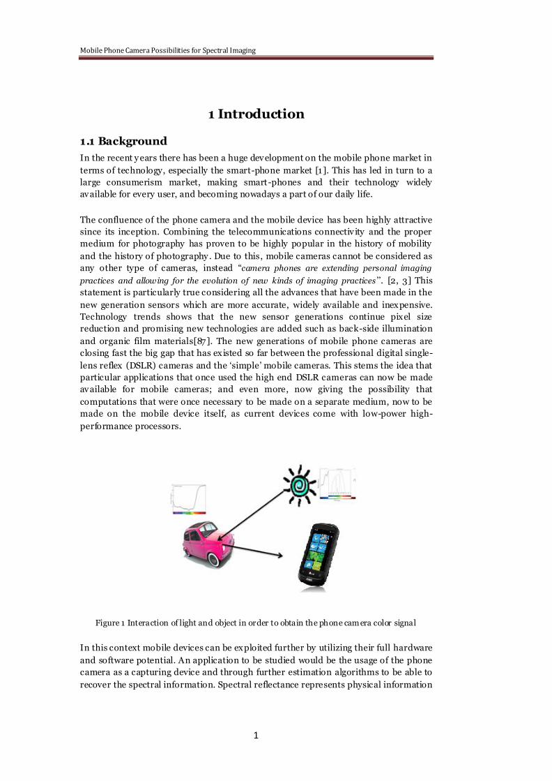
Figure 1 Interaction of light and object in order to obtain the phone camera color signal
In this context mobile devices can be exploited further by utilizing their full hardware
and software potential. An application to be studied would be the usage of the phone
camera as a capturing device and through further estimation algorithms to be able to
recover the spectral information. Spectral reflectance represents physical information
Mobile Phone Camera Possibilities for Spectral Imaging
2
of an object surface [4]. Literature provides a myriad of possibilities in the recovery of
spectral reflectance. These include: liquid cry stal tunable filters (LCTF) coupled with
a monochrome camera [5], a six-position filter wheel containing absorption filters
couple with a monochrome camera, and a two -position filter slider containing
absorption filters coupled with a color-filter array (CFA) color camera [6], direct sight
spectrograph [7], or dichroic mirrors devices [8]. Said dev ices can provide indeed
accurate results, but also have some drawbacks such as high costs, high -level of
expertise needed to utilize them, and they may require extra hardware for imaging
which can become problematic in some types of environments. Compared to the
above mentioned devices the smart-phone cameras provide an inexpensive, fast,
practical and widely available solution.
Object information, when captured by a phone camera is captured in terms of a color
signal, which is a product of the object spectral reflectance and the illuminant, as
shown in Figure1. Therefore the cameras output is illuminant dependent. An increase
of applications in many different fields requires the objects true spectral reflectance
information which is independent on the v iewing illuminant, hence the importance of
providing the spectral information from the cameras RGB response values . So far
applications tested on high end DSLR cameras provide good results in terms of
reflectance estimation which leads to believe that the the new sensor technologies in
current smart-phone cameras will also provide good results. Examples of fields where
DSLR cameras give good results and can also be extended to smart -phone cameras
include: fruit identification and quality control, material classificatio n [10], artwork
imaging [11, 14], printing industry [12], medical imaging [13], or distinguishing
between metameric pairs [10]. A pair is called metameric if they match in color under
the same type of illuminant, but if the illuminant is changed the match in color
doesn‘t hold true anymore, due to the different spectral reflectance that the pairs
have[16]. An example of usage for smartphones in distinguishing metamerism might
be in the leather industry: a customer wants to buy a leather jacket and matching pair
of shoes. The items might look color-wise the same in the shop, but under a different
environment where the illuminant is changed the items will look different. In such a
case we see the importance of hav ing spectral information of the objects so we can
ascertain if the color of jacket and the shoe are the same. The smart-phone through its
camera and processing sy stem can be used to obtain an estimate of the spectral
reflectance and thus a solution to the problem. This allows spectral imaging in the
pocket of every user of mobile dev ices.
1.2 Research Objective
RGB camera devices are generally considered metameric imaging devices, in
opposition to spectral imaging which uses a high number of spectral channels,
ranging from values higher than there to several hundred, depending on the
applications [17]. Metameric imaging is considered in respect to the human v isual
sy stem (HVS). The HVS uses its three ty pes of cone receptors to process the spectral
data over the visible (VIS) wavelength range of 380 -780 nm in order to produce a
three-channel color image. This image is considered metameric because, independent
on the type of the illuminant, the same color response is produced in the three
integrated channels. The same can said about a color RGB camera where we obtain
the same image color output from a variety of illuminants [17]. Because of this we can
Mobile Phone Camera Possibilities for Spectral Imaging
3
assert that the RGB camera was not built with the idea of recovering spectral
information but rather for obtaining an image that is visually pleasant for the
observer [18]. Furthermore due to a short number of spectral bands with broad
bandwidth and the need for aprioric data information, RGB devices are not perfectly
suitable for measuring spectral information. However due to the rapid development
of new technologies in color cameras and also a broad number of reflectance
estimation techniques, the RGB devices provide a practical, inexpensive and fast
solution in recovering spectral information.
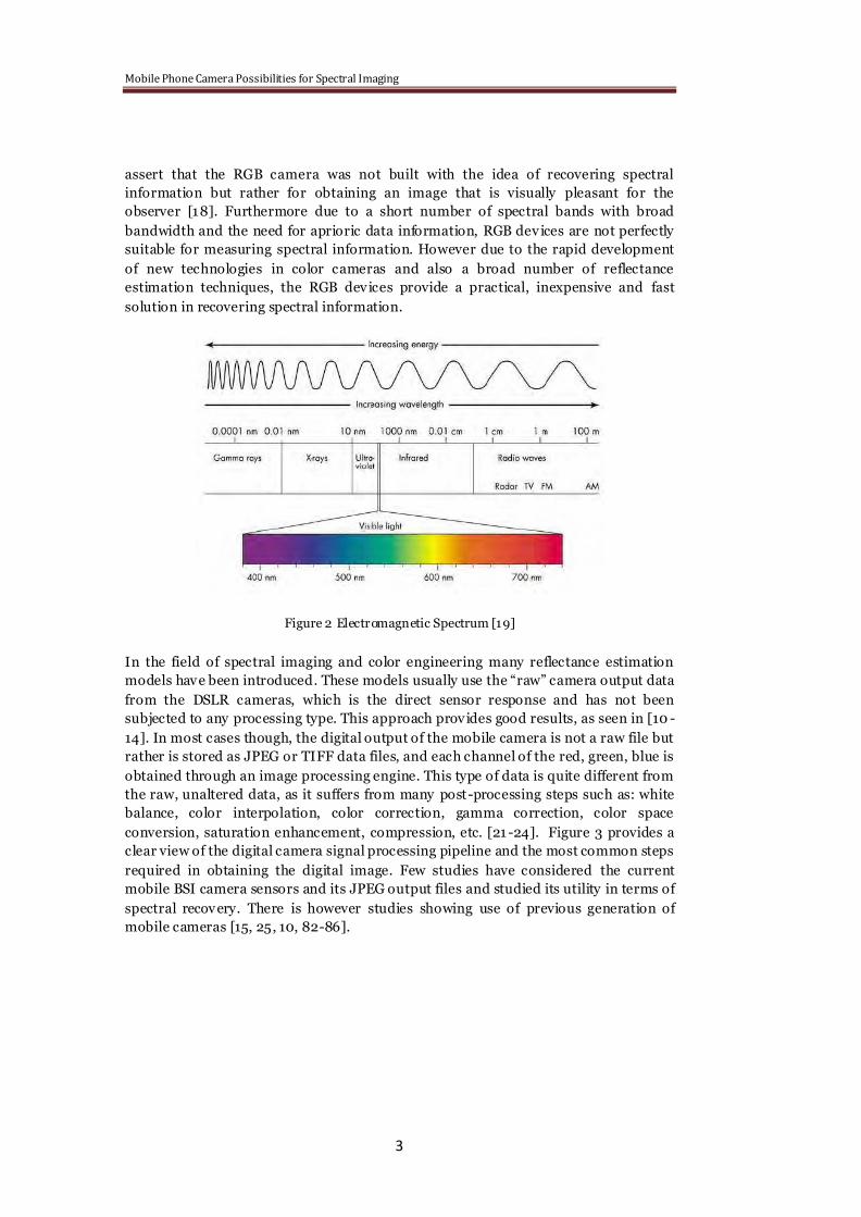
Figure 2 Electromagnetic Spectrum [19]
In the field of spectral imaging and color engineering many reflectance estimation
models have been introduced. These models usually use the ―raw‖ camera output data
from the DSLR cameras, which is the direct sensor response and has not been
subjected to any processing type. This approach provides good results, as seen in [10 -
14]. In most cases though, the digital output of the mobile camera is not a raw file but
rather is stored as JPEG or TIFF data files, and each channel of the red, green, blue is
obtained through an image processing engine. This type of data is quite different from
the raw, unaltered data, as it suffers from many post-processing steps such as: white
balance, color interpolation, color correction, gamma correction, color space
conversion, saturation enhancement, compression, etc. [21 -24]. Figure 3 provides a
clear view of the digital camera signal processing pipeline and the most common steps
required in obtaining the digital image. Few studies have considered the current
mobile BSI camera sensors and its JPEG output files and studied its utility in terms of
spectral recovery. There is however studies showing use of previous generation of
mobile cameras [15, 25, 10, 82-86].

Mobile Phone Camera Possibilities for Spectral Imaging
4
Figure 3 Digital camera signal processing pipeline [20]
Questions are raised concerning how the steps involved in the making of a digital
image affect reflectance estimation models. For this, four smart-phone cameras, two
DSLR cameras and one simple commercial digital camera were used for testing. The
estimation methods employed were: linear fitting v ia least square (also known as the
pseudo-inverse method [26, 27 , 29, 30, 31 and 32], or simply as linear Wiener
estimation method [14]) and an improvement of the first by using multivariate
polynomial fitting via least squares [28, 32].
Further related questions:
Question 1: Why do we choose a professional DSLR instead of a simple mobile phone
camera, or a simple daily usage camera, in terms of reflectance estimation?
Question 2: What ty pe of reflectance estimation models can be used?
Question 3: Are the image processing steps important factors?
Question 4: Is the level of compression an important factor?
Question 5: Spectral imaging in your pocket?
By answering these questions the thesis intends to provide a study in the practicality
and usefulness of the information obtained as output from the smart-phone RGB
camera compared to the raw data information used from DSLR cameras in terms of
spectral imaging estimates and it will be used to provide a basis in future applications
such mobile imaging in artworks, cultural heritage, medical imaging, etc.
1.3 Outline and Contents of the thesis
The thesis is structured in six chapters, including the introduction chapter. Chapters
two and three include literature rev iew and theoretical backgrounds. Chapter two
reviews the mechanism of how the human v ision works and its importance to
conventional imaging. Also discussed are sensors in digital cameras with focus on the
current sensors in smartphones. Spectral imaging and its importance is also
presented in this chapter. Chapter three describes spectral estimation techniques such
as Wiener estimation method, liniar estimation metho d and multivariate poly nomial
method via least squares. Also different spectral metrics are discussed. Furthermore
JPEG compression algorithm is also presented. Chapter four presents data

Mobile Phone Camera Possibilities for Spectral Imaging
5
acquisition devices, acquisition setups employed in the current work also data
preprocessing methods. Chapter five presents the main results of the work and also
discussion upon the results is ensured. The final chapter of the thesis is Chapter six
where conclusions are drawn and future work is presented.

Mobile Phone Camera Possibilities for Spectral Imaging
6
Mobile Phone Camera Possibilities for Spectral Imaging
7
2. Literature Review
2.1 Human Vision
In this chapter mechanism of the human eye and v isual perception are presented as
the human v ision sy stem is considered a base for conventional imaging.
Light is radiation in the form of electromagnetic waves that make vision possible to
the human eye. Human eye is sensitive only to a narrow band of the electromagnetic
spectrum, the v isible spectrum having the spectral range between 380 to 780 nm [67].
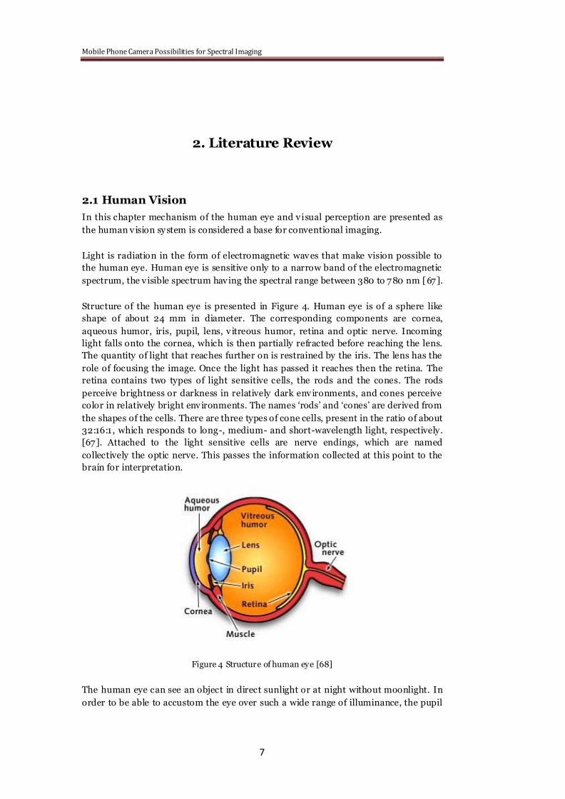
Structure of the human eye is presented in Figure 4. Human eye is of a sphere like
shape of about 24 mm in diameter. The corresponding components are cornea,
aqueous humor, iris, pupil, lens, v itreous humor, retina and optic nerve. Incoming
light falls onto the cornea, which is then partially refracted before reaching the lens.
The quantity of light that reaches further on is restrained by the iris. The lens has the
role of focusing the image. Once the light has passed it reaches then the retina. The
retina contains two types of light sensitive cells, the rods and the cones. The rods
perceive brightness or darkness in relatively dark environments, and cones perceive
color in relatively bright environments. The names ‗rods‘ and ‗cones‘ are derived from
the shapes of the cells. There are three types of cone cells, present in the ratio of about
32:16:1 , which responds to long-, medium- and short-wavelength light, respectively.
[67]. Attached to the light sensitive cells are nerve endings, which are named
collectively the optic nerve. This passes the information collected at this point to the
brain for interpretation.
Figure 4 Structure of human eye [68]
The human eye can see an object in direct sunlight or at night without moonlight. In
order to be able to accustom the eye over such a wide range of illuminance, the pupil

Mobile Phone Camera Possibilities for Spectral Imaging
8
adjusts the quantity of light reaching the retina by vary ing its size. Thus the change in
pupil diameter is insufficient for full control of the quantity of light. Accordingly, the
rods and cones share the function by changing the responsiv ity of the retina. In a
relatively bright environment, the cones alone function to give what is called photopic
v ision. In a relatively dark environment, the rods alone function to realize what is
called scotopic v ision. In environments having an intermediate brightness between
photopic v ision and scotopic v ision, both the cones and the rods function to provide
what is called mesopic vision [67 , 69, 70].
In human vision system the colors are sensed by three ty pes of cones named L, M, S.
The cones are maximally sensitive to long (red type of light), medium (green type of
light) or short (blue type of light) wavelengths of light [72]. The wavelength response
curves of the LMS are shown in Figure 5.
Figure 5 Long, Medium and Short cone responses [71]
Responses of the cones can be precisely modeled by a linear sy stem defined as the
spectral sensitivities of the cones, under a fixed set of v iewing conditions [73]. If
spectral power distribution of incident light is given by function f , the linear
model containing the cone responses is given by the following equation:
max
min
1,2,3
ic S f d
i
(2.1)
, where iS represents the spectral sensitiv ity function of the ith type cone,
min max, represent the minimum and maximum wavelength.
If N uniform wavelengths are sampled over the v isible region range then the model
will be:
Mobile Phone Camera Possibilities for Spectral Imaging
9
1
1,2,3
N
i i i
i
c S f d
i
(2.2)
, where i is the uniformly spaced wavelength.
2.2 Digital Camera Sensors
The process of creating a digital image is very similar to that of human visual system
in that both respond to light and in particular images. Thus light, reflected from an
object, enters the camera and passes through a set of lens. The lens focuses the light
into a set of sensor and filter (such as the Bay er filter), after which the light is
recorded electronically. Therefore in the process of creating a digital image the sensor
plays an important role.
This chapter presents operating principles of two of the most used sensor type in
digital cameras namely: CCD and CMOS image sensors. Also focus in this chapter is
given to BSI type sensors as they represent presently the most used sensors in today‘s
smartphone cameras. [57-60]
2.2.1 CCD sensor
The Charged Coupled Device (CCD) was invented in 1970 by Willard Boy le and
George Smith at Bell Laboratories, USA [64].
A CCD is an electrical dev ice that is used to create images of objects, store information
(analogous to the way a computer stores information), or transfer electrical charge (as
part of larger device). It receives as input light from an object or an electrical charge.
The CCD takes this optical or electronic input and converts it into an electronic signal
- the output. The electronic signal is then processed by some other equipment and/or
software to either produce an image or to give the user valuable information [63].
CCDs are integrated circuits (ICs), that allow light to fall on the silicon chip (or die) a
small glass window is inserted in front of the chip. Conventional ICs are usually
encapsulated in a black plastic body to primarily provide mechanical strength, but
this also shields them from light, which can affect their normal operation. CCDs are
manufactured using metal-oxide-semiconductor (MOS) fabrication techniques, and
each pixel can be thought of as a MOS capacitor that converts photons (light) into
electrical charge, and stores the charge prior to readout [64].
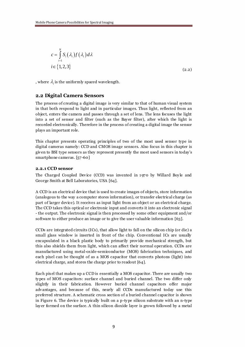
Each pixel that makes up a CCD is essentially a MOS capacitor. There are usually two
ty pes of MOS capacitors: surface channel and buried channel. The two differ only
slightly in their fabrication. However buried channel capacitors offer major
advantages, and because of this, nearly all CCDs manufactured today use this
preferred structure. A schematic cross section of a buried channel capacitor is shown
in Figure 6. The device is typically built on a p-ty pe silicon substrate with an n-type
lay er formed on the surface. A thin silicon dioxide layer is grown followed by a metal
Mobile Phone Camera Possibilities for Spectral Imaging
10
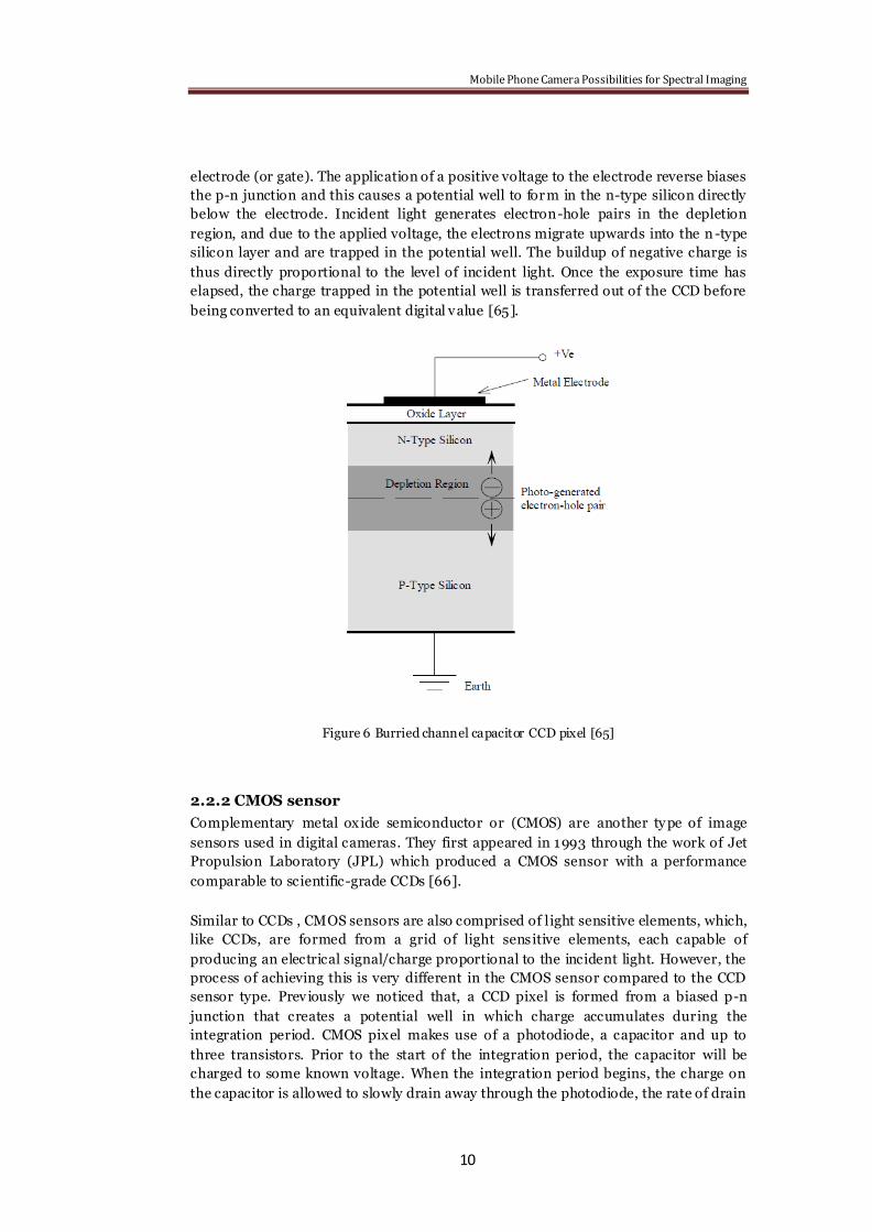
electrode (or gate). The application of a positive voltage to the electrode reverse biases
the p-n junction and this causes a potential well to form in the n-type silicon directly
below the electrode. Incident light generates electron-hole pairs in the depletion
region, and due to the applied voltage, the electrons migrate upwards into the n -type
silicon layer and are trapped in the potential well. The buildup of negative charge is
thus directly proportional to the level of incident light. Once the exposure time has
elapsed, the charge trapped in the potential well is transferred out of the CCD before
being converted to an equivalent digital value [65].
Figure 6 Burried channel capacitor CCD pixel [65]
2.2.2 CMOS sensor
Complementary metal oxide semiconductor or (CMOS) are another ty pe of image
sensors used in digital cameras. They first appeared in 1993 through the work of Jet
Propulsion Laboratory (JPL) which produced a CMOS sensor with a performance
comparable to scientific-grade CCDs [66].
Similar to CCDs , CMOS sensors are also comprised of light sensitive elements, which,
like CCDs, are formed from a grid of light sensitive elements, each capable of
producing an electrical signal/charge proportional to the incident light. However, the
process of achieving this is very different in the CMOS sensor compared to the CCD
sensor type. Prev iously we noticed that, a CCD pixel is formed from a biased p-n
junction that creates a potential well in which charge accumulates during the
integration period. CMOS pixel makes use of a photodiode, a capacitor and up to
three transistors. Prior to the start of the integration period, the capacitor will be
charged to some known voltage. When the integration period begins, the charge on
the capacitor is allowed to slowly drain away through the photodiode, the rate of drain
Mobile Phone Camera Possibilities for Spectral Imaging
11
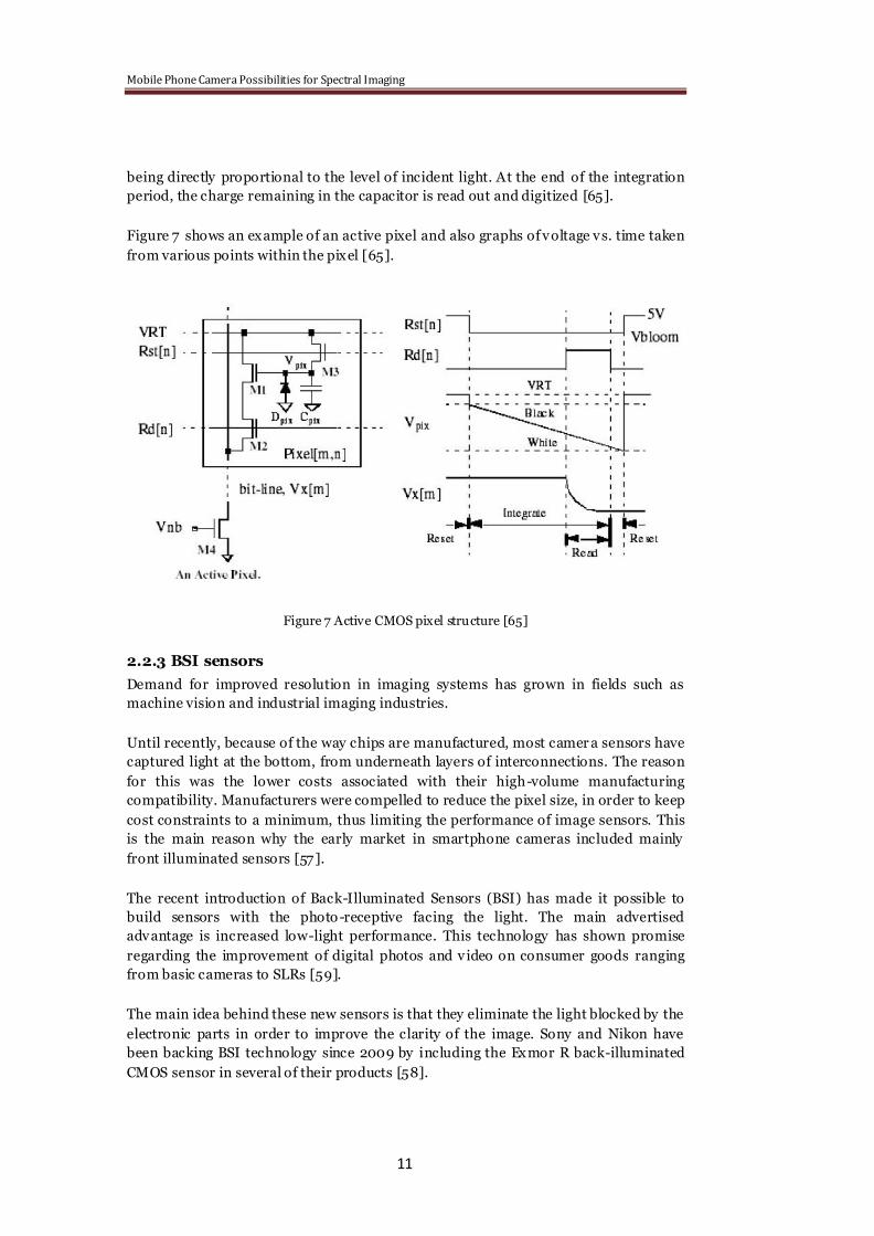
being directly proportional to the level of incident light. At the end of the integration
period, the charge remaining in the capacitor is read out and digitized [65].
Figure 7 shows an example of an active pixel and also graphs of voltage vs. time taken
from various points within the pixel [65].
Figure 7 Active CMOS pixel structure [65]
2.2.3 BSI sensors
Demand for improved resolution in imaging systems has grown in fields such as
machine vision and industrial imaging industries.
Until recently, because of the way chips are manufactured, most camer a sensors have
captured light at the bottom, from underneath layers of interconnections. The reason
for this was the lower costs associated with their high-volume manufacturing
compatibility. Manufacturers were compelled to reduce the pixel size, in order to keep
cost constraints to a minimum, thus limiting the performance of image sensors. This
is the main reason why the early market in smartphone cameras included mainly
front illuminated sensors [57].
The recent introduction of Back-Illuminated Sensors (BSI) has made it possible to
build sensors with the photo -receptive facing the light. The main advertised
advantage is increased low-light performance. This technology has shown promise
regarding the improvement of digital photos and v ideo on consumer goods ranging
from basic cameras to SLRs [59].
The main idea behind these new sensors is that they eliminate the light blocked by the
electronic parts in order to improve the clarity of the image. Sony and Nikon have
been backing BSI technology since 2009 by including the Exmor R back-illuminated
CMOS sensor in several of their products [58].
Mobile Phone Camera Possibilities for Spectral Imaging
12
Presently, the structure of the image sensors is similar in structure with human and
most animal eyes in the way that the photosensitive part is on the side furthest away
from the light. This makes it easier to provide circulation to the energy -hungry rods
and cones cells found in biological eyes while permitting easy removal of debris from
the organ [60]. In the case of artificial sensors silicon is used for both the chip and the
transformation of photons into electrical energy. It is therefore easy to create the
photosensitive areas in the substrate silicon and stack the electronics on top while
leav ing openings in the wiring over each photosite (pixel) to allow light to p ass
through. However, as camera resolutions have increased, pixel sizes have decreased
resulting in more and more of the surface area of the sensor being covered by wiring,
resulting in less and less light reaching the photosites [60]. This lead to a need to find
a way to move the photosensitive region to the top of the chip, allowing it to gather
more light. Optimized back-illuminated sensors can extend the spectral range down
to deep-UV levels while maintaining high and stable responsiv ity. They also improve
the system‘s performance by capturing more light, which improves the signal -to-noise
ratio, increases the inspection speed and minimizes damaging UV exposure to
delicate semiconductor devices.
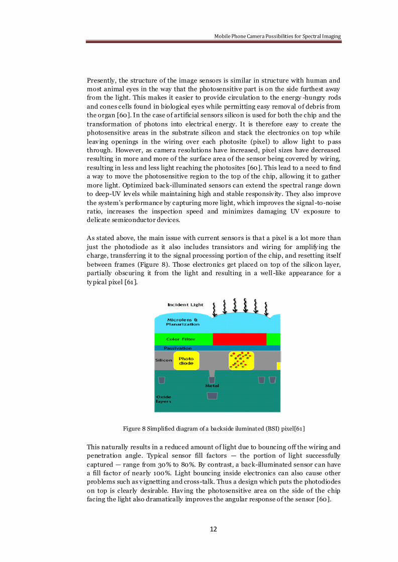
As stated above, the main issue with current sensors is that a pixel is a lot more than
just the photodiode as it also includes transistors and wiring for amplify ing the
charge, transferring it to the signal processing portion of the chip, and resetting itself
between frames (Figure 8). Those electronics get placed on top of the silicon layer,
partially obscuring it from the light and resulting in a well-like appearance for a
ty pical pixel [61].
Figure 8 Simplified diagram of a backside iluminated (BSI) pixel[61]
This naturally results in a reduced amount of light due to bouncing off the wiring and
penetration angle. Typical sensor fill factors — the portion of light successfully
captured — range from 30% to 80%. By contrast, a back-illuminated sensor can have
a fill factor of nearly 100%. Light bouncing inside electronics can also cause other
problems such as v ignetting and cross-talk. Thus a design which puts the photodiodes
on top is clearly desirable. Having the photosensitive area on the side of the chip
facing the light also dramatically improves the angular response of the sensor [60].
Mobile Phone Camera Possibilities for Spectral Imaging
13
The main difficulty in manufacturing sensors with the photo receptors on top comes
from the fabrication process. In order to have a silicon layer on top of it is necessary
to build a chip the same way as a traditional front-illuminated and then place another
lay er of silicon substrate on top and flip the entire silicon sandwich over. After that,
the original silicon base, now on top, has to be thinned to make it act as a light -
sensitive layer. In order to achieve this, the back layer of a BI sensor has to be
between 5-10 microns thick (less than 1% of the original thickness). Given that the
wafer-thinning operation is performed as the last step, any y ield loss significantly
affects cost. Because the BSI wafer has been inverted, the incident light in BSI first
strikes the silicon volume away from the photodiode where light may be lost from
crosstalk due to diffusion to adjoining pixels or lost due to diffusion and
recombination at the back interface. Blue light in particular is susceptible to this
phenomenon, resulting in decreased blue QE and increased crosstalk. These issues
can be addressed with the introduction of a deeper photodiode to capture the blue
light and through advanced backside processing [61].
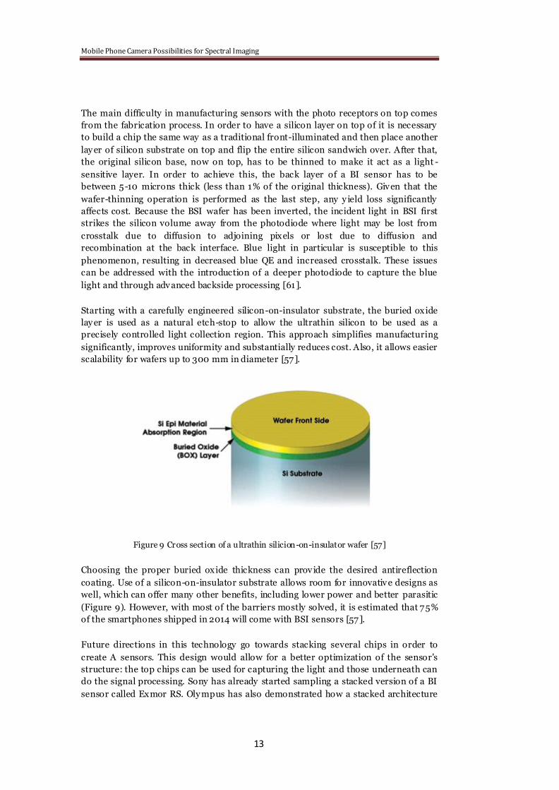
Starting with a carefully engineered silicon-on-insulator substrate, the buried oxide
lay er is used as a natural etch-stop to allow the ultrathin silicon to be used as a
precisely controlled light collection region. This approach simplifies manufacturing
significantly, improves uniformity and substantially reduces cost. Also, it allows easier
scalability for wafers up to 300 mm in diameter [57].
Figure 9 Cross section of a ultrathin silicion-on-insulator wafer [57]
Choosing the proper buried oxide thickness can provide the desired antireflection
coating. Use of a silicon-on-insulator substrate allows room for innovative designs as
well, which can offer many other benefits, including lower power and better parasitic
(Figure 9). However, with most of the barriers mostly solved, it is estimated that 75%
of the smartphones shipped in 2014 will come with BSI sensors [57].
Future directions in this technology go towards stacking several chips in order to
create A sensors. This design would allow for a better optimization of the sensor's
structure: the top chips can be used for capturing the light and those underneath can
do the signal processing. Sony has already started sampling a stacked version of a BI
sensor called Exmor RS. Oly mpus has also demonstrated how a stacked architecture
Mobile Phone Camera Possibilities for Spectral Imaging
14
can create new possibilities. The Olympus design transfers all of the charge off the
sensor at once, to the lower, shielded layer, where they can then be read out
accurately [60].
2.3 Spectral imaging
Spectral imaging is a technology that provides images at multiple wavelengths and
hence generates precise optical spectra at every pixel. Spectral imaging is a growing
field, made possible through the new developments in technology such as in new
detectors, optics, and spectral imaging techniques. A variety of technologies are now
available for use and spectral imaging is a well established technique. [80]
A great deal of attention is given to spectral imaging lately and this is due to the
numerous applications areas where spectral information is needed. The primary
application for spectral imaging was in the area of remote sensing and terrestrial
military. Nowaday s however spectral imaging is used in different type of domains
such environmental monitoring, material analysis, computer v ision and industrial
quality control. Also spectral information was used in medical imaging such as to
analy ze skin color, to simulate adaptation in the human v ision system or to improve
color reproduction of electronic endoscopes. Furthermore we see spectral imaging
used in cultural heritage as it is a noninvasive type of approach [81].
2.3.1 Spectral Imaging Devices
There are different approaches for obtaining spectral images. One approach acquires
a sequence of images at different wavelengths. This can be implemented by using
multiple-position filter wheel containing absorption filters couple d with a
monochrome camera [6]. Another approach captures the spectrum by scanning line
the line the imaged object, where each line contains the complete spectrum. This ty pe
of implementation requires an imaging spectrograph coupled to a monochrome
camera. The whole spectral imaged is obtained after the object is scanned completely
either by moving the object or either by moving the spectral dev ice in small
increments. [7]
Other approaches include liquid crystal tunable filters (LCTF) coupled with a
monochrome camera which uses electronically controlled liquid crystal elements to
select and transmitted wavelength range of interest while blocking all others [5].
Even more another approach in retriev ing the spectral image can be the usage of
acousto-optical tunable filter (AOTF) is an electronic dispersive dev ice based on the
principle of interaction between an ordinary ray (o -ray ), an extraordinary ray (e-ray ),
and a traveling acoustic wave in a birefringent cry stal [5]
2.3.2 Structure of Spectral Image
Normal spectral imaging color is captured by using three primary colors. Color in a
digital camera is captured through a color filter array (CFA). Conventional CFA is
represented by a three color Bayer filter, where each color is formed through red,
green and blue filters [53, 54].
Mobile Phone Camera Possibilities for Spectral Imaging
15
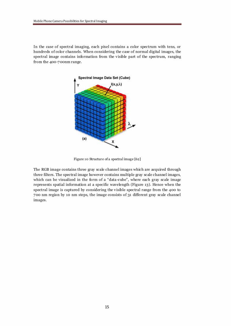
In the case of spectral imaging, each pixel contains a color spectrum with tens, or
hundreds of color channels. When considering the case of normal digital images, the
spectral image contains information from the v isible part of the spectrum, ranging
from the 400-700nm range.
Figure 10 Structure of a spectral image [62]
The RGB image contains three gray scale channel images which are acquired through
three filters. The spectral image however contains multiple gray scale channel images,
which can be visualized in the form of a ―data-cube‖, where each gray scale image
represents spatial information at a specific wavelength (Figure 13). Hence when the
spectral image is captured by considering the v isible spectral range from the 400 to
700 nm region by 10 nm steps, the image consists of 31 different gray scale channel
images.
Mobile Phone Camera Possibilities for Spectral Imaging
16
3. Methodology
3.1 Spectral Estimation Methods
Literature has provided many kinds of spectral estimation methods in order to
reproduce the spectra from three-band or from multispectral images. A small
classification div ides these methods into two categories [26] or three c ategories [27],
where the pseudo-inverse model is considered as the third category . The first two
categories include: Wiener estimation model, which minimizes the mean square
errors (MSEs) between the real measured spectral reflectance and the estimated
reflectance spectra, and the second is the finite-dimensional linear model, where the
spectral reflectance is represented as linear combination of ortho -normal basis
vectors.
Wiener estimation model requires three matrixes: the autocorrelation matrix of
spectral reflectance, the spectral sensitiv ity of the camera sensor and the system
noise, in order to recover the spectral reflectance. The system noise and the
autocorrelation matrix represent a crucial point in characterizing the efficiency of the
estimation as seen in [34].
The finite-dimensional linear model takes advantage of the representation of the
linear model, where the spectral reflectance is represented as a weighted sum of a set
of basis functions, which can be obtained by applying principal component analy sis
(PCA) to an aprioric set of known spectra. [27]
The above model types require prior knowledge of the spectral sensitiv ities and the
spectral power distribution (SPD) of the illumination. Measuring these spectral
characteristics accurately is not a straightforward task, thus development of new
estimation methods appeared. Such is the linear estimation model via least squares
also known as the pseudo-inverse model, which is a modification of the Wiener
estimation model that uses regression analysis between the known spectral
reflectance‘s and the sensor responses. Imai-Berns model represents another model
that doesn‘t assume prior knowledge of the spectral sensitiv ities and the SPD of the
illumination. It also uses regression analy sis between the output of the sensor and the
weight column vectors for the ortho-normal basis vectors. [26]
Digital camera devices capture the spectrum by filtering the incoming color signal
through a set of color filters [29]. Mathematically the interaction between the
spectrum of the object, illumination and the digital camera can be modeled as follows:
( ) E( ) ( )
1,...,
i i iP R S d e
i m
(3.1)
Mobile Phone Camera Possibilities for Spectral Imaging
17
, where (x, y)iP represents the response of the digital, (x, y; )R is the spectral
reflectance of an object, ( )E is the spectral power distribution of the illuminant,
S ( )i represents the spectral camera sensitivity of the thi camera channel , ie is the
camera sy stem noise and is denoted as the wavelength variable. In practice, we
have only three camera channels in a digital camera, namely the Red, Green and Blue
channel, thus the m in equation 1 is equal to three.
3.1.1 Wiener estimation
Considering the case of the digital camera, the spectral reflectance of the image object
is sampled uniformly at n intervals in the spectral range of 400 to 700 nm. Equation 1
can be more easily represented in a vec tor and matrix form as:
x SEr e (3.2)
, where x is the camera response vector in a 3 1 column vector form, r is an 1n
element column vector defined as 1(R( ),...,R( ))T
nr and denotes the spectral
reflectance of the objects, S is the spectral sensitiv ities matrix defined by a 3 n
matrix , E represents a n n matrix corresponding to the illuminants SPD, and e is
the 3 1 column vector denoting the noise. The noise is considered to be coming not
only from the sensors but also the measurement errors of the spectral characteristics
of the sensor, illumination and spectral reflectance. [26]
Reconstructing the r spectrum from the camera responses involves using aprioric
information of the sensors, illumination and the reflectances of objects. This aprioric
information is used so that the model learns from these in order to provide an
estimation of the original r spectrum.
Let M SE be a simpler representation of the product of the spectral sensitiv ity of
the camera and the SPD of the illumination.
The solution in reconstructing the reflectance spectrum is finding an estimation
matrix W that minimizes the mean square error of the Euclid norm of E r Wx ,
where .E is defined as the expectation.
Matrix W is defined as:
1
T T
SS SS EEW R M MR M R
(3.3)
, where
T
SSR E rr , T
EER E ee (3.4)
Mobile Phone Camera Possibilities for Spectral Imaging
18
In equation3.3 and equation 3.4 T represents the transpose of a matrix, SSR is the
autocorrelation matrix of the spectral reflectance of the test or learning samples and
EER represents the autocorrelation matrix of noise. If the autocorrelation matrices are
equal to the actual autocorrelation matrices of noise and spectral reflectance, then the
value of the MSE will be minimized [26]. Unfortunately this doesn‘t stand true
because prior knowledge of noise is usually not available, and it is usually guessed.
The recovered spectrum has the form:
r̂ Wx (3.6)
The solution for Wiener estimation model involves the usage of aprioric knowledge
which makes this method quite difficult. In a practical case, a more elegant solution is
offered by the linear model via least squares fitting that recovers the spectral
reflectance without the prior knowledge of the spectral sensitiv ities of the sensors and
the SPD of the illumination [26].
3.1.2 Linear model via least squares fitting
The linear model v ia least squares represents a simple solution which is to build a
mapping from camera responses to reflectance in order to minimize the least square
error for a training set of known reflectance functions with known camera responses
[41].
Thus we have a training set:
3, , , , 1...n
i i i iS x y x y i m (3.7 )
This training set consists of the pairs of vectors corresponding to the camera
responses ix and the spectral reflectance iy . The traditional setting method is
characterized as estimating a set of three-dimensional scalar-valued functions as
,
1,...
i iy f x
i n
(3.8)
, where iy represents the reflectance at wavelength.
With every new set of camera responses x the reflectance is estimated by the
associated functions 1 2, ,... nf x f x f x . [27]
In the studied case there are only three channels corresponding to the camera
responses, namely the red, green and blue channels. The input vector now becomes:

Mobile Phone Camera Possibilities for Spectral Imaging
19
, ,T
x R G B (3.9)
In practical cases x includes the constant variable 1, thus the input vector has the
form:
, , ,1T
x R G B (3.10)
Given the input vector x we have the linear form:
,f x w x (3.11)
The solution of w is searched so that the mean square error of the following is
minimized:
2
,L f S r Xw (3.12)
, where X represents an 4m matrix having each row as expressed in eq. and where
r represents the reflectance vector, both X and r coming from the training set
[27].
The solution for will have the form:
1
ˆ T Tv X X X r
(3.13)
, where v̂ is the estimated spectral reflectance.
The estimates obtained in equation 3.13 and equation 3.6 are different because the
estimates of the correlation and that of the noise are different [29].
3.1.3 Polynomial model via least squares fitting
The linear model can be extended to a nonlinear case by employ ing the poly nomial
spread of the camera responses. [27 , 28]
The once linear function transforms to a nonlinear functions as:
, qf x w x (3.14)
, where the q x represents the input values now having the poly nomial spread to
the qth degree of the polynomial terms.
The solution in this case will have the form:
Mobile Phone Camera Possibilities for Spectral Imaging
20
1
ˆ T Tv P P P r
(3.15)
, where v̂ is the estimated spectral reflectance and P is a matrix having each row an
input vector of q
ix
3.1.4 Special considerations
Because of the large amount of information present in the data-cube, the storage size
of a spectral image is quite high amounting to hundreds of megaby tes or even
gigabytes. This can pose a problem when considering creating an application for a
smartphone that retrieves and stores the spectral data. Therefore special
consideration needs to be given for this. Usually, the spectral image data-cube is
saved to user specific binary formats, or different compression methods are used like
PCA in order to reduce dimensionality [54-56].
Another fact to consider is also memory allocation, as estimation methods work using
large matrixes in order to construct the data cube. There has to be a good balance
between correct allocation of memory resources and time spent in obtaining the
spectral image. So considering the case of a 20 megabit sensor we will have a
4000x5000x 3 RGB image. When transforming it to a spectral image considering the
v isible range of 400-700nm with 5 nm sampling we will get 4000x5000x61 data
cube. This occupies roughly more than 1Gb of memory space. Reducing dimensions
of the spectral image data cube can be done by choosing an optimal sampling. This is
of course illuminant [79] and application dependent. Also as previously mentioned
reducing the spectral data can be done by different compression methods like PCA.
3.2 Spectral metrics
In order to measure the distance between the original spectral reflectance and the
estimated spectral reflectance two different spectral metrics were used: goodness of
fit coefficient (GFC) and root mean square error (RMSE). These metrics are good for
distinguishing between metamers. However they do not consider human vision [40]
3.2.1 Goodness of fit coefficient (GFC)
In order to evaluate the goodness of the mathematical reconstruction, the GFC is used
which is based on Schwartz inequality:
2 2
( ) R ( )
( ) ( )
m i e i
i
m i e i
i i
R
GFC
R R
(3.16)
, where, m iR represents the original measured spectral reflectance at wavelength
i and e iR represents the estimated spectral reflectance at wavelength i .

Mobile Phone Camera Possibilities for Spectral Imaging
21
The GFC coefficient takes values ranging from 0 to 1 , with the value 1 having the
meaning that the estimate represents the exact spectra of the original. For
colorimetric accuracy e iR needs the GFC to be higher than 0.995. For good
spectral fit the GFC needs to be 0.999GFC and 0.9999GFC is considered as
almost perfect fit. [35-39]
3.2.2 Root Mean Square Error (RMSE)
RMSE represents another way of computing the differences between the original
spectra and the estimated spectra. As the name implies it gives the squared error loss
by calculating the square root of mean square error [35-39].
2
1
1 N
m e
i
RMSE R RN
(3.17)
Where mR represents the original spectra and eR represents the estimated
spectra and N is the number of elements in the spectra.
3.2.3 CIELAB Color Difference
Psy chophysical experiments have shown that the human ey e‘s sensitivity to light is
not linear [50]. The RGB and also the XY Z color spaces defined by the CIE
(International Commission on Illumination) are linearly related to the spectral power
distribution of the colored light. When changing the tristimulus values XY Z (or RGB)
of a color stimulus, the observer will perceive a difference in color only after a certain
amount, equal to the Just Noticeable Difference (JND). [50] In both RGB and XY Z
spaces the JND depends on the location in the color spaces. In order to address this
CIELAB space was proposed in 1976 by CIE, having the quantities: [51]
* 116 16
* 500
* 500
n
n n
n n
YL f
Y
X Ya f f
X Y
Y Zb f f
Y Z
(3.18)
13
3
3
24
116
841 16 24
108 116 116
n n n
n n n
K K Kf if
K K K
K K Kf if
K K K
(3.19)

Mobile Phone Camera Possibilities for Spectral Imaging
22
, where K can be each of the three tristimulus values , ,X Y Z and , , Zn n nX Y
represent the tristimulus values of a perfect reflecting diffuser under the same
illuminant. The values are normalized so that 100nY .
*L represents the lightness of a color going from a scale of 0 (black) to 100 (white).
Chromaticity can be represented on a 2D diagram where *a is the degree of red
versus green and *b is degree of y ellow versus blue.
CIELAB color difference is defined in the CIELAB color space system as the Euclidean
distance between two color stimulus with the following equation [46, 47 , 51]:
2 2 2
* * * *E L a b (3.20)
1 2
1 2
1 2
* * *
*
* * *
L L L
a a a
b b b
(3.21)
Practical interpretations of *E can be found in tables in the works of Hardeberg et
al [49] and Abrado et al [48], and can be seen in tables below:
Table 1 Interpretation of CIELAB color difference by Abrado et al [48]
Table 2 Interpretation of CIELAB color difference by Hardeberg et al [49]
E Effect
<3 Hardly perceptible
E Effect
0-1 Limit of perception
1-3 Very good quality
3-6 Good quality
6-10 Sufficient
>10 Insufficient
Mobile Phone Camera Possibilities for Spectral Imaging
23
3-6 Perceptible, but acceptable
>6 Not acceptable
3.2.4 CIEDE2000 Color difference
CIEDE2000 is a CIE recommended color difference formula, which includes new
terms to improve the predicted color difference in the blue region and for neutral
colors, for pairs of samples with small to moderate color differences [52]. CIEDE2000
is based on the CIELAB color space. Given a pair of color values in CIELAB space
2
1*,a *, *i i i i
L b , the CIEDE2000 color difference between them is calculated using
the equation:
22 2
2000 T
L L C C H H C C H H
L C H C HCIEDE R
k S k S k S k S k S
(3.22)
3.3 JPEG compression
As previously mentioned the output of the majority of commercial digital cameras is
presented in different formats rather than the direct sensor output. Usual formats
that can be found imply some form of compression such as JPEG data ty pe, PNG data
ty pe or TIFF data type.
Smartphone cameras also include as the main form of output JPEG ty pe images.
Newer generation of camera sensors are being developed such to allow access to the
RAW information. Currently only the Nokia PureView technology allows the direct
sensor output [75]. However still the main form as output remains the JPEG image as
it represents a storage cost effective compression method that discards information
that the human eye cannot easily see.
JPEG is the international standard for the effective compression of the still digital
images. It includes specifications for both- lossless and lossy compression algorithm.
JPEG lossy standard was designed with the consideration to diminish the high
frequency component of the image frame that human eye cannot detect easily. This
was done due to the fact that human v ision detects better changes in the light
intensity rather than changes in color space. JPEG standard tends to be more
aggressive towards the compression of the color-part (chrominance) of the image
instead of the gray -scale part of the image. Compression in JPEG is realized mainly
due to the quantization effect, which when implemented results in the loss of part of
the image information and hence degradation of image quality occurs [74].
Mobile Phone Camera Possibilities for Spectral Imaging
24
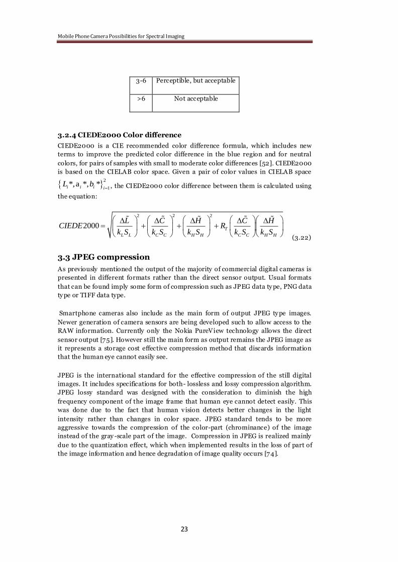
Figure 11 Steps in implementing the JPEG encoder [77]
Figure 10 presents the steps involved in implementing the JPEG encoder. The first
step involves transforming the image to an appropriate luminance/c hrominance color
space such as Y CbCr space. The gray scale, low frequency component Y contains the
luminance information of the image to which human eyes are sensitive. The other
channels Cb and Cr are chrominance channels that contain the high frequency co lor
information to which human eyes are not sensitive in the blue and red region. As the
chrominance channels contain less relevant information they are usually subsampled.
Typical patterns (as seen in Figure 11) include subsampling the chrominance channel
in vertical direction (4:2:2), or horizontal direction (4:4:0) or both (4:2:0) [76]. All
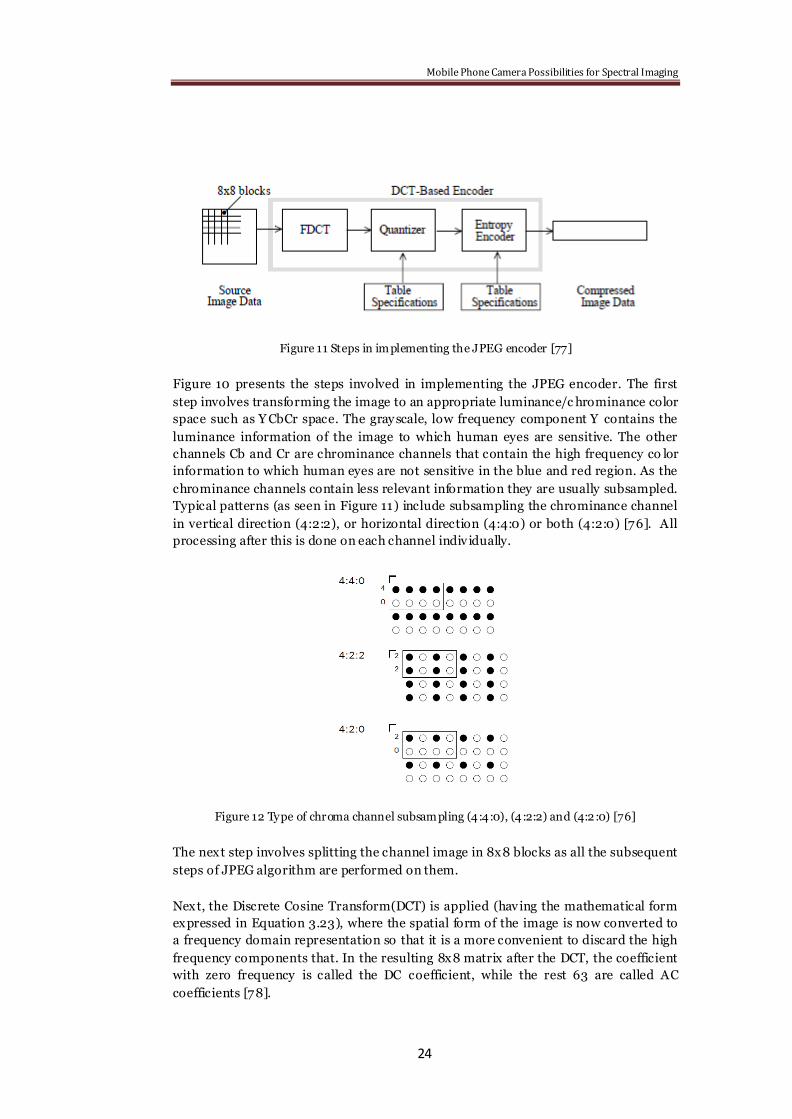
processing after this is done on each channel indiv idually.
Figure 12 Type of chroma channel subsampling (4:4:0), (4:2:2) and (4:2:0) [76]
The next step involves splitting the channel image in 8x8 blocks as all the subsequent
steps of JPEG algorithm are performed on them.
Next, the Discrete Cosine Transform(DCT) is applied (having the mathematical form
expressed in Equation 3.23), where the spatial form of the image is now converted to
a frequency domain representation so that it is a more convenient to discard the high
frequency components that. In the resulting 8x8 matrix after the DCT, the coefficient
with zero frequency is called the DC coefficient, while the rest 63 are called AC
coefficients [78].
Mobile Phone Camera Possibilities for Spectral Imaging
25
7 7
0 0
2 1 2 11, , cos cos
4 16 16x y
x u y vF u v C u C v f x y
(3.23)
, where
7 7
0 0
2 1 2 11, , cos cos
4 16 16u v
x u y vf x y C u C v F u v
, and
1, , 0
2
, 1
C u C v for u v
C u C v otherwise
After this follows the most important step in the JPEG compression, namely the
quantization, as it is the principal source of lossiness. This is done by dividing each of
the DCT coefficients by a quantization table and then rounding the result. Thus the
high frequency DCT coefficients are quantized more heavily, in comparison with the
low frequency coefficients, as the play a smaller role in the image representation and
cannot be easily perceived by human eyes. Quantization tables are defined as user
specific. [78]
After quantization, the DC coefficient is treated separately from the 63 AC
coefficients. The DC coefficient is a measure of the average value of the 64 image
samples. The DC coefficient is encoded as the difference from the DC term of the
previous block in the encoding order. After all of the quantized coefficients are
ordered into the ―zig-zag‖ sequence. This ordering helps to facilitate entropy coding
by placing low-frequency before high-frequency coefficients [77].
The final processing step is entropy coding. This step achieves additional compression
losslessly by encoding the quantized DCT coefficients more compactly based on their
statistical characteristics. The JPEG proposal specifies two entropy coding methods -
arithmetic coding and Huffman coding, where the latter is used in baseline sequential
JPEG encoding [77].

Mobile Phone Camera Possibilities for Spectral Imaging
26
Figure 13 Steps in implementing the JPEG decoder[77]
In order to decode the JPEG compressed data, the JPEG decoder is needed. This
basically reiterates all the mentioned processing steps in a reverse order (as seen in
Figure 12). Thus we will have an entropy decoder, a dequantizer, and an Inverse
Discrete Cosine Transform (IDCT) that will reconstruct the image data

Mobile Phone Camera Possibilities for Spectral Imaging
27
Mobile Phone Camera Possibilities for Spectral Imaging
28
4 Measurements
4.1 Data acquisition
4.1.1 Specim ImSpector (V10E)
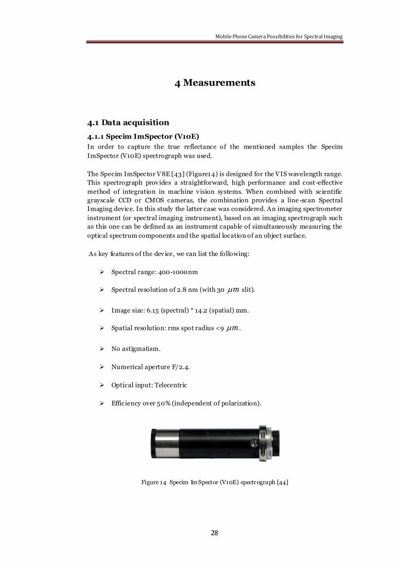
In order to capture the true reflectance of the mentioned samples the Specim
ImSpector (V10E) spectrograph was used.
The Specim ImSpector V8E [43] (Figure14) is designed for the VIS wavelength range.
This spectrograph provides a straightforward, high performance and cost -effective
method of integration in machine v ision systems. When combined with scientific
grayscale CCD or CMOS cameras, the combination provides a line -scan Spectral
Imaging device. In this study the latter case was considered. An imaging spectrometer
instrument (or spectral imaging instrument), based on an imaging spectrograph such
as this one can be defined as an instrument capable of simultaneously measuring the
optical spectrum components and the spatial location of an object surface.
As key features of the dev ice, we can list the following:
Spectral range: 400-1000nm
Spectral resolution of 2.8 nm (with 30 m slit).
Image size: 6.15 (spectral) * 14.2 (spatial) mm.
Spatial resolution: rms spot radius <9 m .
No astigmatism.
Numerical aperture F/2.4.
Optical input: Telecentric
Efficiency over 50% (independent of polarization).
Figure 14 Specim ImSpector (V10E) spectrograph [44]
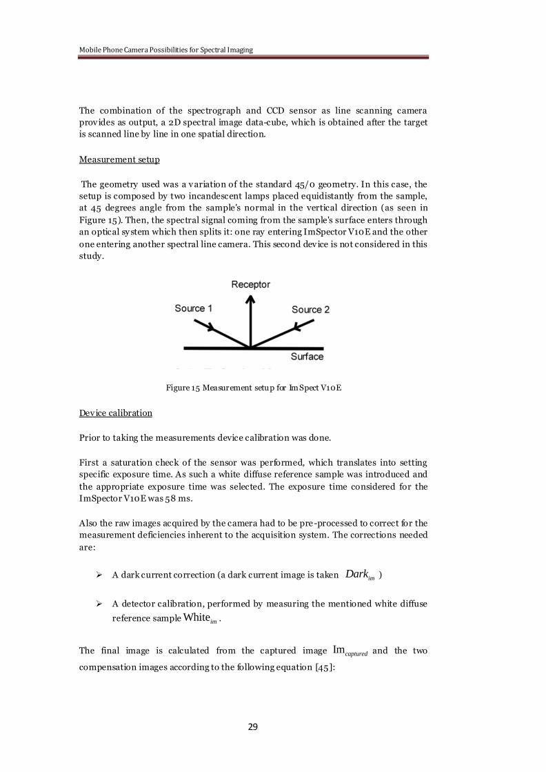
Mobile Phone Camera Possibilities for Spectral Imaging
29
The combination of the spectrograph and CCD sensor as line scanning camera
provides as output, a 2D spectral image data-cube, which is obtained after the target
is scanned line by line in one spatial direction.
Measurement setup
The geometry used was a variation of the standard 45/0 geometry. In this case, the
setup is composed by two incandescent lamps placed equidistantly from the sample,
at 45 degrees angle from the sample's normal in the vertical direction (as seen in
Figure 15). Then, the spectral signal coming from the sample's surface enters through
an optical sy stem which then splits it: one ray entering ImSpector V10E and the other
one entering another spectral line camera. This second device is not considered in this
study.
Figure 15 Measurement setup for ImSpect V10E
Device calibration
Prior to taking the measurements device calibration was done.
First a saturation check of the sensor was performed, which translates into setting
specific exposure time. As such a white diffuse reference sample was introduced and
the appropriate exposure time was selected. The exposure time considered for the
ImSpector V10E was 58 ms.
Also the raw images acquired by the camera had to be pre -processed to correct for the
measurement deficiencies inherent to the acquisition system. The corrections needed
are:
A dark current correction (a dark current image is taken imDark )
A detector calibration, performed by measuring the mentioned white diffuse
reference sample Whiteim .
The final image is calculated from the captured image Imcaptured and the two
compensation images according to the following equation [45]:
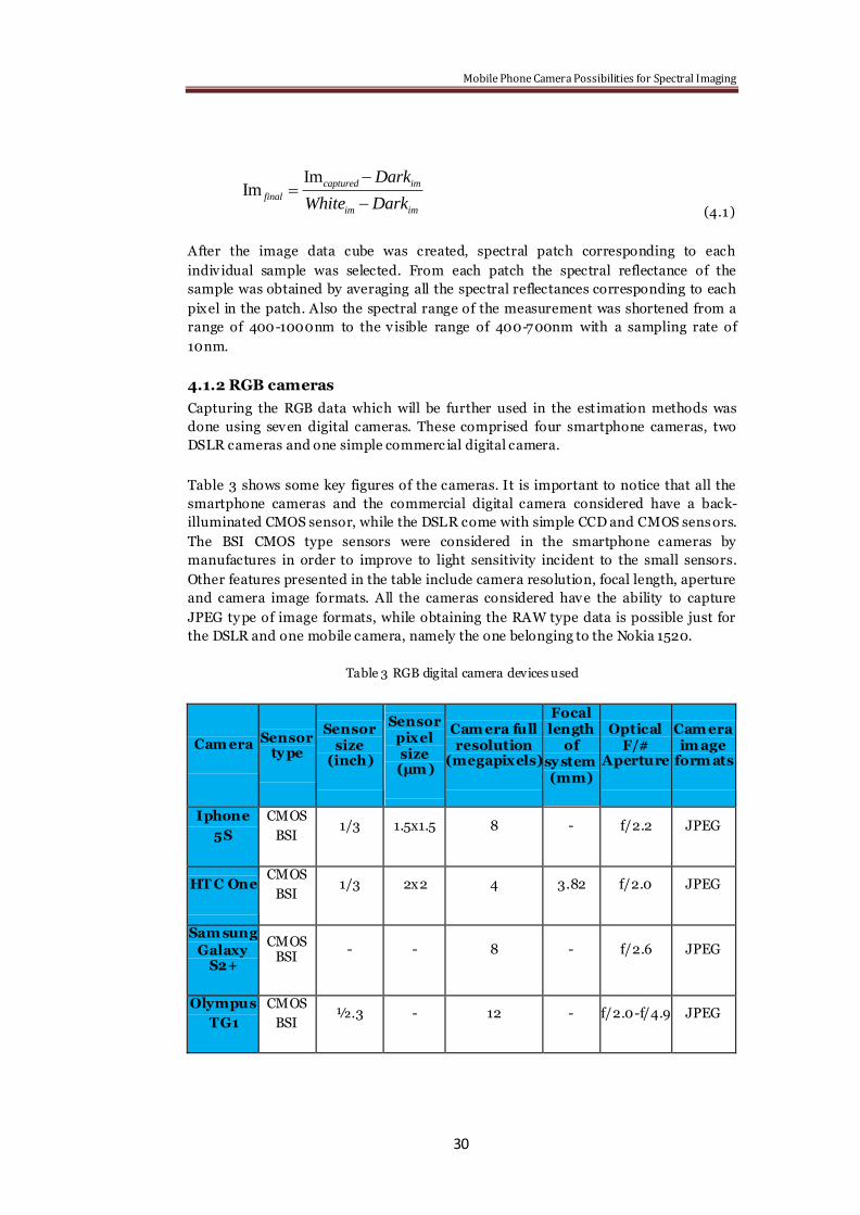
Mobile Phone Camera Possibilities for Spectral Imaging
30
ImIm
captured im
final
im im
Dark
White Dark
(4.1)
After the image data cube was created, spectral patch corresponding to each
indiv idual sample was selected. From each patch the spectral reflectance of the
sample was obtained by averaging all the spectral reflectances corresponding to each
pixel in the patch. Also the spectral range of the measurement was shortened from a
range of 400-1000nm to the v isible range of 400-700nm with a sampling rate of
10nm.
4.1.2 RGB cameras
Capturing the RGB data which will be further used in the estimation methods was
done using seven digital cameras. These comprised four smartphone cameras, two
DSLR cameras and one simple commerc ial digital camera.
Table 3 shows some key figures of the cameras. It is important to notice that all the
smartphone cameras and the commercial digital camera considered have a back-
illuminated CMOS sensor, while the DSLR come with simple CCD and CMOS sens ors.
The BSI CMOS type sensors were considered in the smartphone cameras by
manufactures in order to improve to light sensitivity incident to the small sensors.
Other features presented in the table include camera resolution, focal length, aperture
and camera image formats. All the cameras considered have the ability to capture
JPEG ty pe of image formats, while obtaining the RAW type data is possible just for
the DSLR and one mobile camera, namely the one belonging to the Nokia 1520.
Table 3 RGB digital camera devices used
Cam era Sensor ty pe
Sensor size
(inch)
Sensor pixel size (µm )
Cam era full resolution
(megapixels)
Focal length
of sy stem (mm)
Optical F/#
Aperture
Cam era im age
form ats
Iphone
5S
CMOS
BSI 1/3 1.5x1.5 8 - f/2.2 JPEG
HT C One CMOS
BSI 1/3 2x2 4 3.82 f/2.0 JPEG
Sam sung
Galaxy S2+
CMOS BSI
- - 8 - f/2.6 JPEG
Olympus
TG1
CMOS
BSI ½.3 - 12 - f/2.0-f/4.9 JPEG

Mobile Phone Camera Possibilities for Spectral Imaging
31
Nokia 1520
CMOS BSI
½.5 1.12x1.12 20 26 f/2.4 JPEG, 10 bit RAW
Nikon D80
CCD 23.6x15.8 milimeter
- 10 - f/3/5-f/5.6 JPEG,
TIFF, 12 bit RAW
Nikon D800
CMOS 35.9x24
milimeter 0 36 - f/3/5-f/5.6
JPEG, TIFF, 14 bit RAW
Measurement setup
The RGB images were capture in the light booth using a D65 illumination, and the
surround was kept dark. The geometry considered was 45/0, where the samples were
illuminated at a 45 degree angle, while the measurements of the samples were
captured at a 0 degree angle (as seen in Figure 16). The geometry was chosen so that
the specular components of the samples did not appear in the images.
When capturing the images some parameters were fixed such as the ISO set to 100 (in
the HTC One case this was not possible even though the setting allowed so), distance
from target to 40cm and auto white balancing. Other parameters were considered
inherent as it was not possible to change them such as the resolution, exposure time,
and aperture. Only the DSLR cameras allowed changing aperture and exposure time,
thus the values selected were so that the ratio between the exposure time and
aperture was similar to the ones obtained in the mobile cameras. All numerical values
can be seen in Table 4.
The images considered in tests were both JPEG and RAW in the cases where the
camera allowed so.
All the parameters considered were established so that it was po ssible to provide
similar results in the image capturing process, which will allow further on a
comparison between the different devices.
Figure 16 Measurement setup for RGB cameras
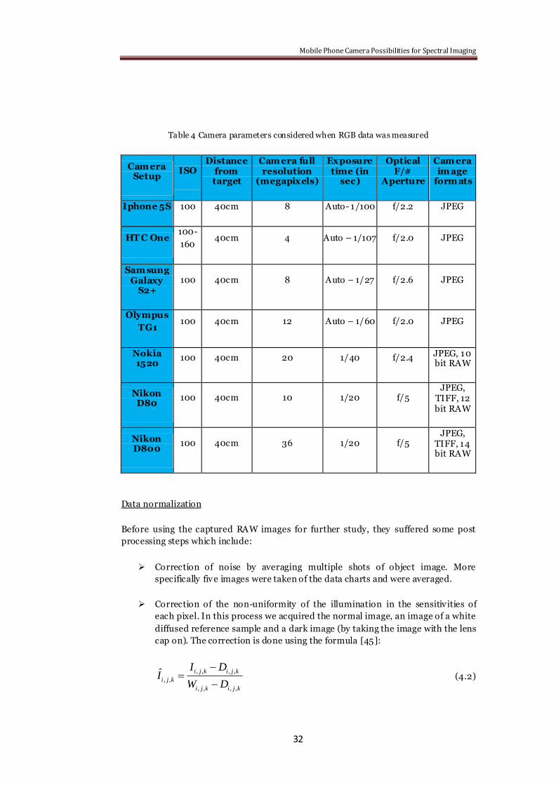
Mobile Phone Camera Possibilities for Spectral Imaging
32
Table 4 Camera parameters considered when RGB data was measured
Cam era Setup
ISO Distance
from target
Cam era full resolution
(megapixels)
Exposure time (in
sec)
Optical F/#
Aperture
Cam era im age
form ats
Iphone 5S 100 40cm 8 Auto- 1/100 f/2.2 JPEG
HT C One 100-
160 40cm 4 Auto – 1/107 f/2.0 JPEG
Sam sung Galaxy
S2+ 100 40cm 8 Auto – 1/27 f/2.6 JPEG
Olympus
TG1 100 40cm 12 Auto – 1/60 f/2.0 JPEG
Nokia 1520
100 40cm 20 1/40 f/2.4 JPEG, 10 bit RAW
Nikon D80
100 40cm 10 1/20 f/5 JPEG,
TIFF, 12 bit RAW
Nikon D800
100 40cm 36 1/20 f/5 JPEG,
TIFF, 14 bit RAW
Data normalization
Before using the captured RAW images for further study, they suffered some post
processing steps which include:
Correction of noise by averaging multiple shots of object image. More
specifically five images were taken of the data charts and were averaged.
Correction of the non-uniformity of the illumination in the sensitiv ities of
each pixel. In this process we acquired the normal image, an image of a white
diffused reference sample and a dark image (by taking the image with the lens
cap on). The correction is done using the formula [45]:
, , , ,
, ,
, , , ,
ˆ i j k i j k
i j k
i j k i j k
I DI
W D
(4.2)
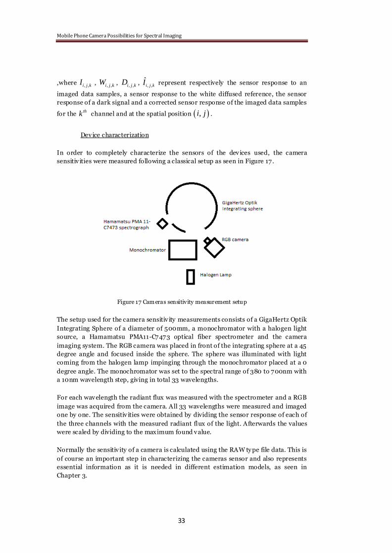
Mobile Phone Camera Possibilities for Spectral Imaging
33
,where , ,i j kI , , ,i j kW , , ,i j kD , , ,ˆi j kI represent respectively the sensor response to an
imaged data samples, a sensor response to the white diffused reference, the sensor
response of a dark signal and a corrected sensor response of the imaged data samples
for the thk channel and at the spatial position ,i j .
Device characterization
In order to completely characterize the sensors of the dev ices used, the camera
sensitiv ities were measured following a classical setup as seen in Figure 17 .
Figure 17 Cameras sensitivity measurement setup
The setup used for the camera sensitiv ity measurements consists of a GigaHertz Optik
Integrating Sphere of a diameter of 500mm, a monochromator with a halogen light
source, a Hamamatsu PMA11-C7473 optical fiber spectrometer and the camera
imaging system. The RGB camera was placed in front of the integrating sphere at a 45
degree angle and focused inside the sphere. The sphere was illuminated with light
coming from the halogen lamp impinging through the monochromator placed at a 0
degree angle. The monochromator was set to the spectral range of 380 to 700nm with
a 10nm wavelength step, giving in total 33 wavelengths.
For each wavelength the radiant flux was measured with the spectrometer and a RGB
image was acquired from the camera. All 33 wavelengths were measured and imaged
one by one. The sensitiv ities were obtained by dividing the sensor response of each of
the three channels with the measured radiant flux of the light. Afterwards the values
were scaled by dividing to the maximum found value.
Normally the sensitiv ity of a camera is calculated using the RAW ty pe file data. This is
of course an important step in characterizing the cameras sensor and also represents
essential information as it is needed in different estimation models, as seen in
Chapter 3.
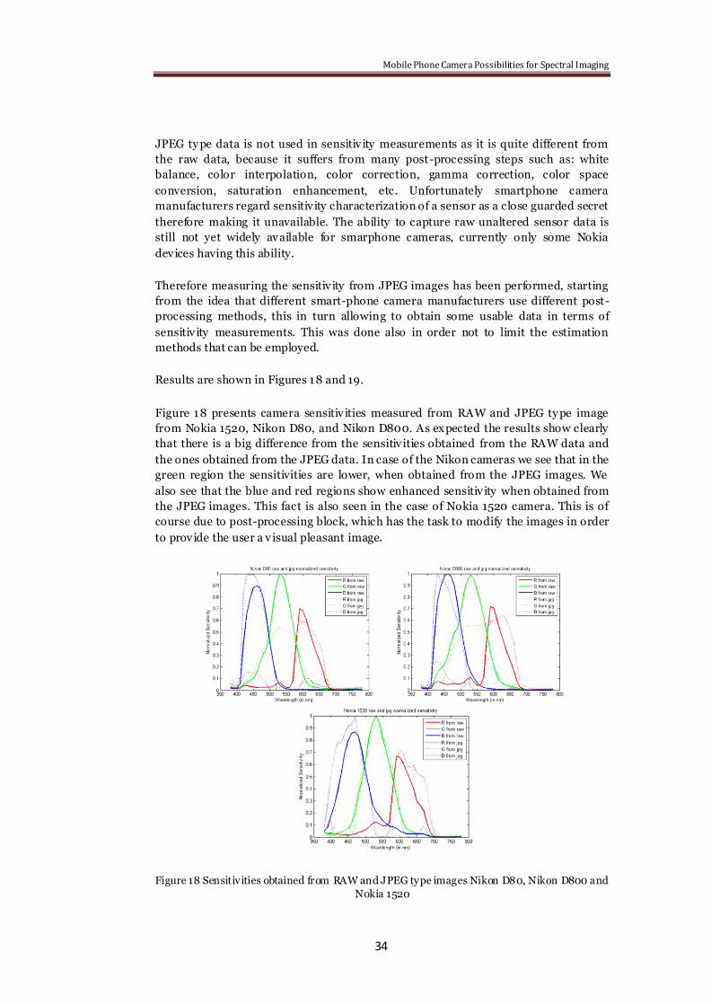
Mobile Phone Camera Possibilities for Spectral Imaging
34
JPEG ty pe data is not used in sensitiv ity measurements as it is quite different from
the raw data, because it suffers from many post-processing steps such as: white
balance, color interpolation, color correction, gamma correction, color space
conversion, saturation enhancement, etc. Unfortunately smartphone camera
manufacturers regard sensitiv ity characterization of a sensor as a close guarded secret
therefore making it unavailable. The ability to capture raw unaltered sensor data is
still not yet widely available for smarphone cameras, currently only some Nokia
dev ices having this ability.
Therefore measuring the sensitiv ity from JPEG images has been performed, starting
from the idea that different smart-phone camera manufacturers use different post-
processing methods, this in turn allowing to obtain some usable data in terms of
sensitiv ity measurements. This was done also in order not to limit the estimation
methods that can be employed.
Results are shown in Figures 18 and 19.
Figure 18 presents camera sensitiv ities measured from RAW and JPEG ty pe image
from Nokia 1520, Nikon D80, and Nikon D800. As expected the results show clearly
that there is a big difference from the sensitiv ities obtained from the RAW data and
the ones obtained from the JPEG data. In case of the Nikon cameras we see that in the
green region the sensitivities are lower, when obtained from the JPEG images. We
also see that the blue and red regions show enhanced sensitiv ity when obtained from
the JPEG images. This fact is also seen in the case of Nokia 1520 camera. This is of
course due to post-processing block, which has the task to modify the images in order
to provide the user a v isual pleasant image.
Figure 18 Sensitivities obtained from RAW and JPEG type images Nikon D80, Nikon D800 and
Nokia 1520
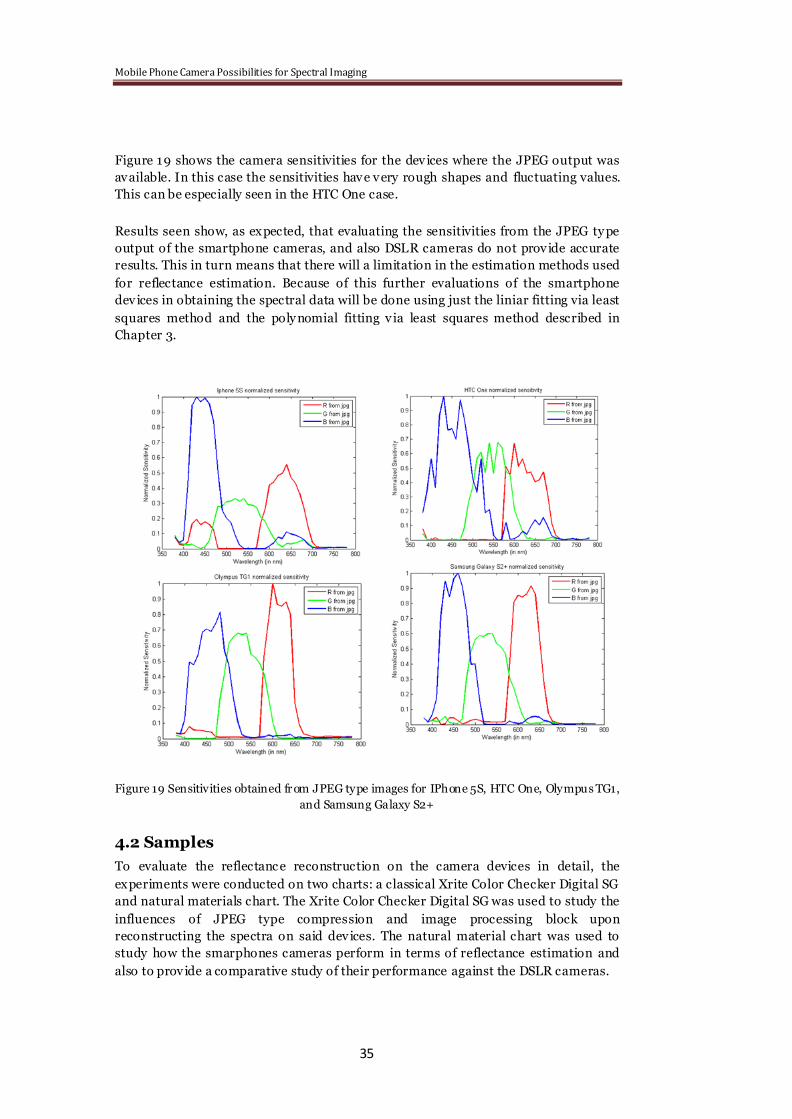
Mobile Phone Camera Possibilities for Spectral Imaging
35
Figure 19 shows the camera sensitivities for the dev ices where the JPEG output was
available. In this case the sensitivities have very rough shapes and fluctuating values.
This can be especially seen in the HTC One case.
Results seen show, as expected, that evaluating the sensitivities from the JPEG ty pe
output of the smartphone cameras, and also DSLR cameras do not provide accurate
results. This in turn means that there will a limitation in the estimation methods used
for reflectance estimation. Because of this further evaluations of the smartphone
devices in obtaining the spectral data will be done using just the liniar fitting via least
squares method and the poly nomial fitting v ia least squares method described in
Chapter 3.
Figure 19 Sensitivities obtained from JPEG type images for IPhone 5S, HTC One, Olympus TG1,
and Samsung Galaxy S2+
4.2 Samples
To evaluate the reflectanc e reconstruction on the camera devices in detail, the
experiments were conducted on two charts: a classical Xrite Color Checker Digital SG
and natural materials chart. The Xrite Color Checker Digital SG was used to study the
influences of JPEG type compression and image processing block upon
reconstructing the spectra on said dev ices. The natural material chart was used to
study how the smarphones cameras perform in terms of reflectance estimation and
also to provide a comparative study of their performance against the DSLR cameras.
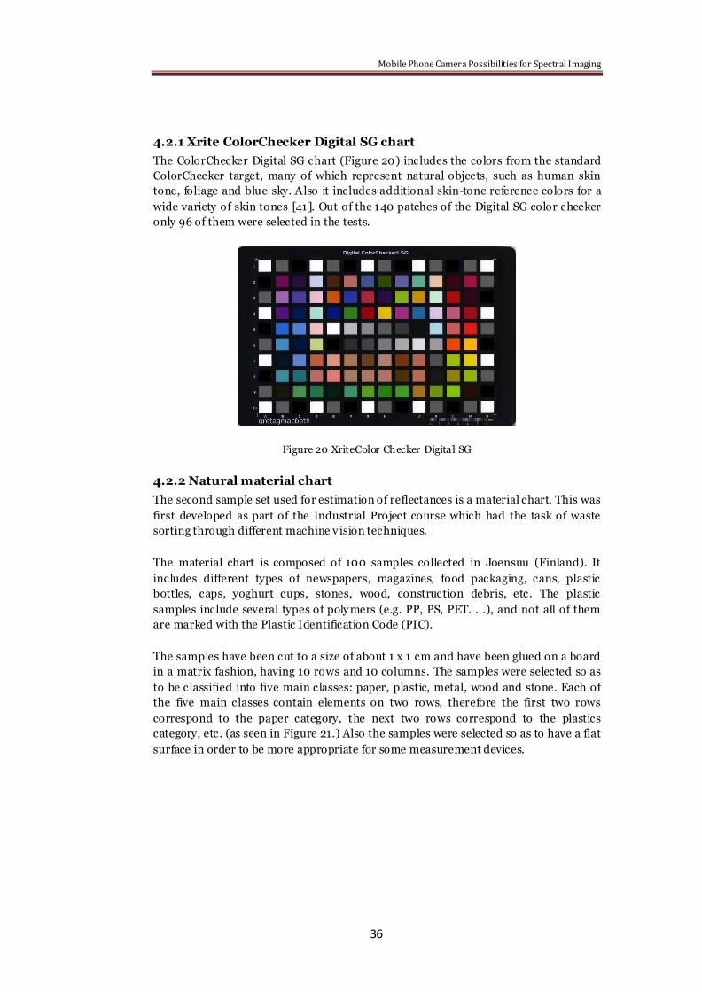
Mobile Phone Camera Possibilities for Spectral Imaging
36
4.2.1 Xrite ColorChecker Digital SG chart
The ColorChecker Digital SG chart (Figure 20) includes the colors from the standard
ColorChecker target, many of which represent natural objects, such as human skin
tone, foliage and blue sky. Also it includes additional skin-tone reference colors for a
wide variety of skin tones [41]. Out of the 140 patches of the Digital SG color checker
only 96 of them were selected in the tests.
Figure 20 XriteColor Checker Digital SG
4.2.2 Natural material chart
The second sample set used for estimation of reflectances is a material chart. This was
first developed as part of the Industrial Project course which had the task of waste
sorting through different machine v ision techniques.
The material chart is composed of 100 samples collected in Joensuu (Finland). It
includes different types of newspapers, magazines, food packaging, cans, plastic
bottles, caps, yoghurt cups, stones, wood, construction debris, etc. The plastic
samples include several types of poly mers (e.g. PP, PS, PET. . .), and not all of them
are marked with the Plastic Identification Code (PIC).
The samples have been cut to a size of about 1 x 1 cm and have been glued on a board
in a matrix fashion, having 10 rows and 10 columns. The samples were selected so as
to be classified into five main classes: paper, plastic, metal, wood and stone. Each of
the five main classes contain elements on two rows, therefore the first two rows
correspond to the paper category, the next two rows correspond to the plastics
category, etc. (as seen in Figure 21.) Also the samples were selected so as to have a flat
surface in order to be more appropriate for some measurement devices.

Mobile Phone Camera Possibilities for Spectral Imaging
37
Figure 21 Natural material chart
In the experiments done samples from both charts were used as testing sets for
estimation, while as training samples for estimation only the XriteColor Checker
Digital SG was used.

Mobile Phone Camera Possibilities for Spectral Imaging
38
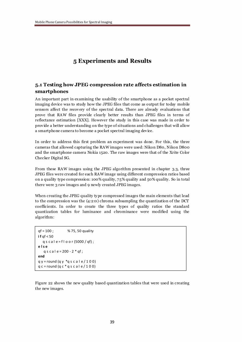
Mobile Phone Camera Possibilities for Spectral Imaging
39
5 Experiments and Results
5.1 Testing how JPEG compression rate affects estimation in
smartphones
An important part in examining the usability of the smartphone as a pocket spectral
imaging device was to study how the JPEG files that come as output for today mobile
sensors affect the recovery of the spectral data. There are already evaluations that
prove that RAW files provide clearly better results than JPEG files in terms of
reflectance estimation [XXX]. However the study in this case was made in order to
provide a better understanding on the type of situations and challenges that will allow
a smartphone camera to become a pocket spectral imaging device.
In order to address this first problem an experiment was done. For this, the three
cameras that allowed capturing the RAW images were used: Nikon D80, Nikon D800
and the smartphone camera Nokia 1520. The raw images were that of the Xrite Color
Checker Digital SG.
From these RAW images using the JPEG algorithm presented in chapter 3.3, three
JPEG files were created for each RAW image using different compression ratios based
on a quality type compression: 100% quality, 75% quality and 50% quality. So in total
there were 3 raw images and 9 newly created JPEG images.
When creating the JPEG quality ty pe compressed images the main elements that lead
to the compression was the (4:2:0) chroma subsampling the quantization of the DCT
coefficients. In order to create the three types of quality ratios the standard
quantization tables for luminance and chrominance were modified using the
algorithm:
Figure 22 shows the new quality based quantization tables that were used in creating
the new images.
qf = 100 ; % 75, 50 quality
i f qf < 50
q s c a l e = f l o o r (5000 / qf) ; e l s e
q s c a l e = 200 - 2 * qf ; end
q y = round (q y *q s c a l e / 1 0 0) q c = round (q c * q s c a l e / 1 0 0)
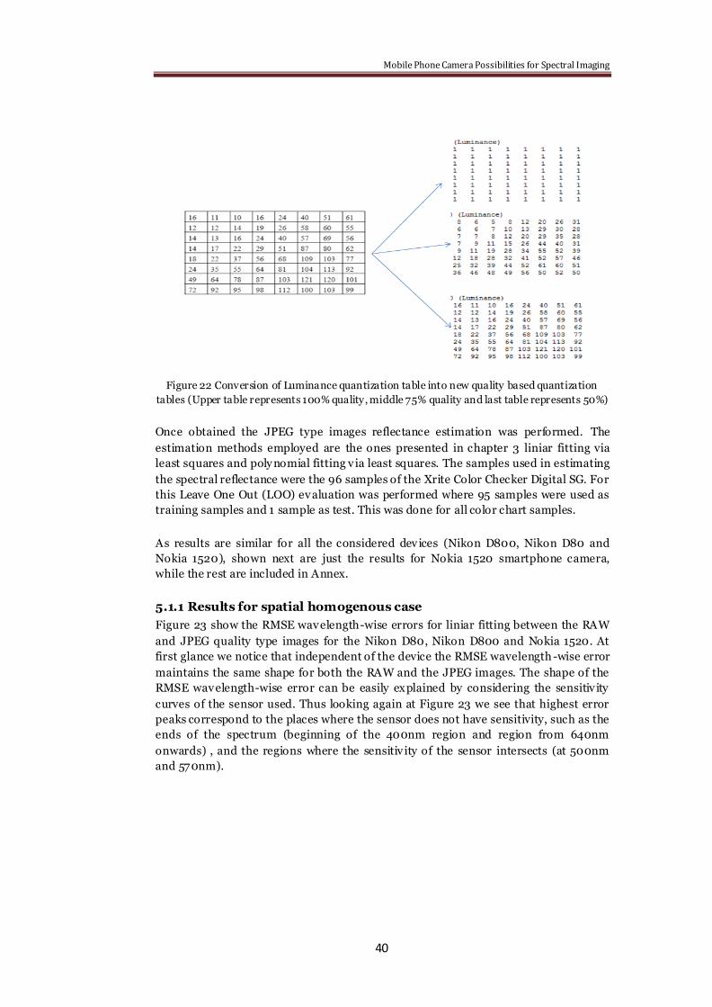
Mobile Phone Camera Possibilities for Spectral Imaging
40
Figure 22 Conversion of Luminance quantization table into new quality based quantization
tables (Upper table represents 100% quality, middle 75% quality and last table represents 50%)
Once obtained the JPEG type images reflectance estimation was performed. The
estimation methods employed are the ones presented in chapter 3 liniar fitting via
least squares and poly nomial fitting v ia least squares. The samples used in estimating
the spectral reflectance were the 96 samples of the Xrite Color Checker Digital SG. For
this Leave One Out (LOO) evaluation was performed where 95 samples were used as
training samples and 1 sample as test. This was done for all color chart samples.
As results are similar for all the considered devices (Nikon D800, Nikon D80 and
Nokia 1520), shown next are just the results for Nokia 1520 smartphone camera,
while the rest are included in Annex.
5.1.1 Results for spatial homogenous case
Figure 23 show the RMSE wavelength-wise errors for liniar fitting between the RAW
and JPEG quality type images for the Nikon D80, Nikon D800 and Nokia 1520. At
first glance we notice that independent of the device the RMSE wavelength -wise error
maintains the same shape for both the RAW and the JPEG images. The shape of the
RMSE wavelength-wise error can be easily explained by considering the sensitiv ity
curves of the sensor used. Thus looking again at Figure 23 we see that highest error
peaks correspond to the places where the sensor does not have sensitivity, such as the
ends of the spectrum (beginning of the 400nm region and region from 640nm
onwards) , and the regions where the sensitiv ity of the sensor intersects (at 500nm
and 570nm).
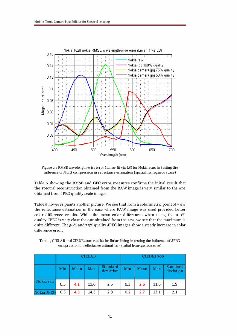
Mobile Phone Camera Possibilities for Spectral Imaging
41
Figure 23 RMSE wavelength-wise error (Liniar fit via LS) for Nokia 1520 in testing the
influence of JPEG compression in reflectance estimation (spatial homogenous case)
Table 6 showing the RMSE and GFC error measures confirms the initial result that
the spectral reconstruction obtained from the RAW image is very similar to the one
obtained from JPEG quality scale images.
Table 5 however paints another picture. We see that from a colorimetric point of v iew
the reflectance estimation in the case where RAW image was used provided better
color difference results. While the mean color differences when using the 100%
quality JPEG is very close the one obtained from the raw, we see that the maximum is
quite different. The 50% and 75% quality JPEG images show a steady increase in color
difference error.
Table 5 CIELAB and CIEDE2000 results for liniar fitting in testing the influence of JPEG
compression in reflectance estimation (spatial homogenous case)
CIELAB CIEDE2000
Min Mean Max Standard deviation
Min Mean Max Standard deviation
Nokia raw 0.5 4.1 11.6 2.5 0.3 2.6 11.6 1.9
Nokia JPEG 0.5 4.3 14.3 2.8 0.2 2.7 13.1 2.1
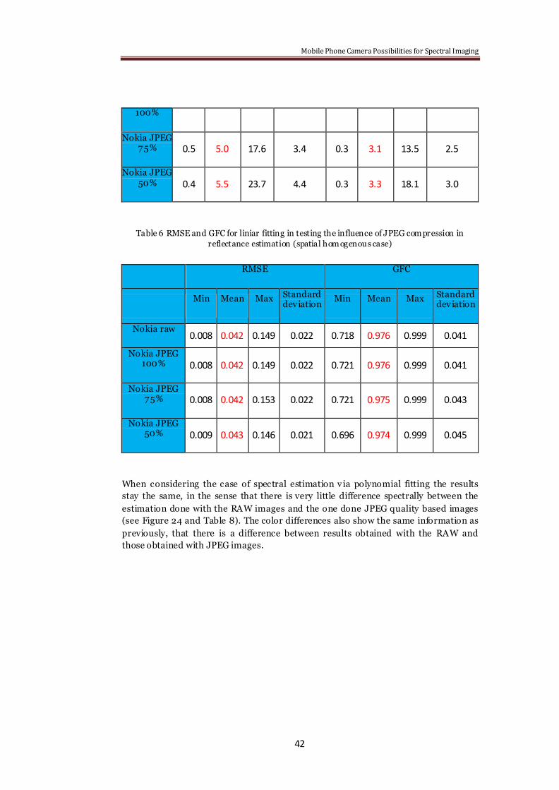
Mobile Phone Camera Possibilities for Spectral Imaging
42
100%
Nokia JPEG 75% 0.5 5.0 17.6 3.4 0.3 3.1 13.5 2.5
Nokia JPEG 50% 0.4 5.5 23.7 4.4 0.3 3.3 18.1 3.0
Table 6 RMSE and GFC for liniar fitting in testing the influence of JPEG compression in
reflectance estimation (spatial homogenous case)
RMSE GFC
Min Mean Max Standard deviation
Min Mean Max Standard deviation
Nokia raw 0.008 0.042 0.149 0.022 0.718 0.976 0.999 0.041
Nokia JPEG 100% 0.008 0.042 0.149 0.022 0.721 0.976 0.999 0.041
Nokia JPEG 75% 0.008 0.042 0.153 0.022 0.721 0.975 0.999 0.043
Nokia JPEG 50% 0.009 0.043 0.146 0.021 0.696 0.974 0.999 0.045
When considering the case of spectral estimation v ia polynomial fitting the results
stay the same, in the sense that there is very little difference spectrally between the
estimation done with the RAW images and the one done JPEG quality based images
(see Figure 24 and Table 8). The color differences also show the same information as
previously, that there is a difference between results obtained with the RAW and
those obtained with JPEG images.
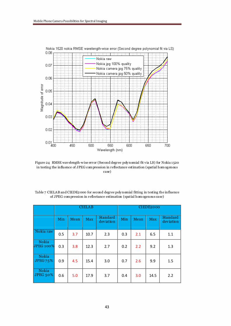
Mobile Phone Camera Possibilities for Spectral Imaging
43
Figure 24 RMSE wavelength-wise error (Second degree polynomial fit via LS) for Nokia 1520
in testing the influence of JPEG compression in reflectance estimation (spatial homogenous
case)
Table 7 CIELAB and CIEDE2000 for second degree polynomial fitting in testing the influence
of JPEG compression in reflectance estimation (spatial homogenous case)
CIELAB CIEDE2000
Min Mean Max Standard deviation
Min Mean Max Standard deviation
Nokia raw 0.5 3.7 10.7 2.3 0.3 2.1 6.5 1.1
Nokia JPEG 100% 0.3 3.8 12.3 2.7 0.2 2.2 9.2 1.3
Nokia JPEG 75% 0.9 4.5 15.4 3.0 0.7 2.6 9.9 1.5
Nokia JPEG 50% 0.6 5.0 17.9 3.7 0.4 3.0 14.5 2.2
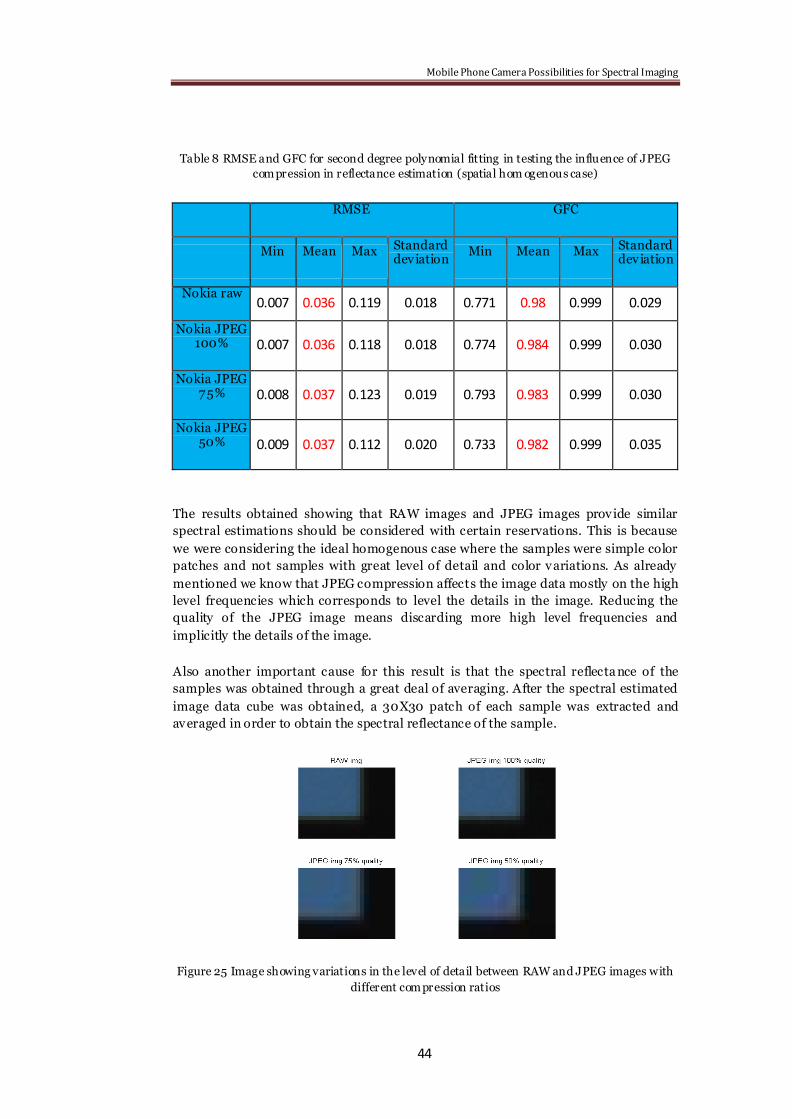
Mobile Phone Camera Possibilities for Spectral Imaging
44
Table 8 RMSE and GFC for second degree polynomial fitting in testing the influence of JPEG
compression in reflectance estimation (spatial hom ogenous case)
RMSE GFC
Min Mean Max Standard deviation
Min Mean Max Standard deviation
Nokia raw 0.007 0.036 0.119 0.018 0.771 0.98 0.999 0.029
Nokia JPEG 100% 0.007 0.036 0.118 0.018 0.774 0.984 0.999 0.030
Nokia JPEG 75% 0.008 0.037 0.123 0.019 0.793 0.983 0.999 0.030
Nokia JPEG 50% 0.009 0.037 0.112 0.020 0.733 0.982 0.999 0.035
The results obtained showing that RAW images and JPEG images provide similar
spectral estimations should be considered with certain reservations. This is because
we were considering the ideal homogenous case where the samples were simple color
patches and not samples with great level of detail and color variations. As already
mentioned we know that JPEG compression affects the image data mostly on the high
level frequencies which corresponds to level the details in the image. Reducing the
quality of the JPEG image means discarding more high level frequencies and
implicitly the details of the image.
Also another important cause for this result is that the spectral reflecta nce of the
samples was obtained through a great deal of averaging. After the spectral estimated
image data cube was obtained, a 30X30 patch of each sample was extracted and
averaged in order to obtain the spectral reflectance of the sample.
Figure 25 Image showing variations in the level of detail between RAW and JPEG images with
different compression ratios
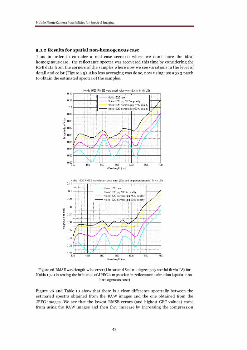
Mobile Phone Camera Possibilities for Spectral Imaging
45
5.1.2 Results for spatial non-homogenous case
Thus in order to consider a real case scenario where we don‘t have the ideal
homogenous case, the reflectance spectra was recovered this time by considering the
RGB data from the corners of the samples where now we see variations in the level of
detail and color (Figure 25). Also less averaging was done, now using just a 3x3 patch
to obtain the estimated spectra of the samples.
Figure 26 RMSE wavelength-wise error (Linear and Second degree polynomial fit via LS) for
Nokia 1520 in testing the influence of JPEG compression in reflectance estimation (spatial non-
homogenous case)
Figure 26 and Table 10 show that there is a clear difference spectrally between the
estimated spectra obtained from the RAW images and the one obtained from the
JPEG images. We see that the lowest RMSE errors (and highest GFC values) come
from using the RAW images and then they increase by increasing the compression
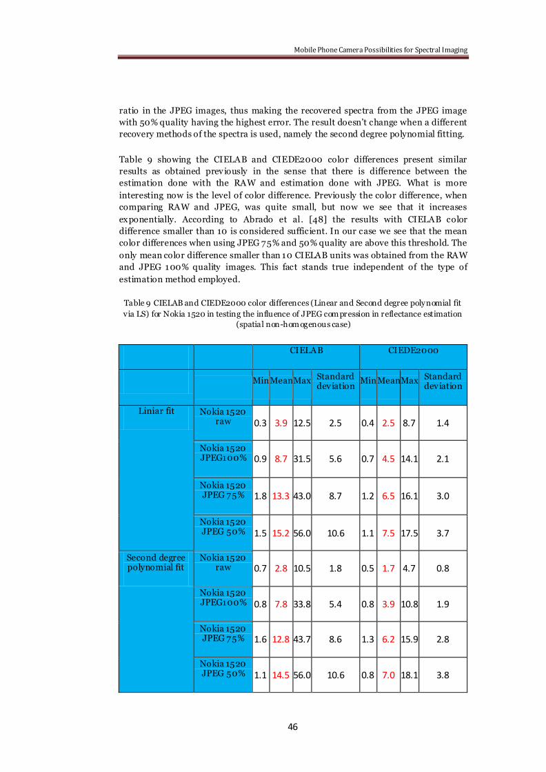
Mobile Phone Camera Possibilities for Spectral Imaging
46
ratio in the JPEG images, thus making the recovered spectra from the JPEG image
with 50% quality having the highest error. The result doesn‘t change when a different
recovery methods of the spectra is used, namely the second degree polynomial fitting.
Table 9 showing the CIELAB and CIEDE2000 color differences present similar
results as obtained prev iously in the sense that there is difference between the
estimation done with the RAW and estimation done with JPEG. What is more
interesting now is the level of color difference. Previously the color difference, when
comparing RAW and JPEG, was quite small, but now we see that it increases
exponentially. According to Abrado et al. [48] the results with CIELAB color
difference smaller than 10 is considered sufficient. In our case we see that the mean
color differences when using JPEG 75% and 50% quality are above this threshold. The
only mean color difference smaller than 10 CIELAB units was obtained from the RAW
and JPEG 100% quality images. This fact stands true independent of the type of
estimation method employed.
Table 9 CIELAB and CIEDE2000 color differences (Linear and Second degree polynomial fit
via LS) for Nokia 1520 in testing the influence of JPEG compression in reflectance estimation
(spatial non-homogenous case)
CIELAB CIEDE2000
Min Mean Max Standard
deviation Min Mean Max Standard
deviation
Liniar fit Nokia 1520 raw 0.3 3.9 12.5 2.5 0.4 2.5 8.7 1.4
Nokia 1520 JPEG100% 0.9 8.7 31.5 5.6 0.7 4.5 14.1 2.1
Nokia 1520 JPEG 75% 1.8 13.3 43.0 8.7 1.2 6.5 16.1 3.0
Nokia 1520 JPEG 50% 1.5 15.2 56.0 10.6 1.1 7.5 17.5 3.7
Second degree polynomial fit
Nokia 1520 raw 0.7 2.8 10.5 1.8 0.5 1.7 4.7 0.8
Nokia 1520 JPEG100% 0.8 7.8 33.8 5.4 0.8 3.9 10.8 1.9
Nokia 1520 JPEG 75% 1.6 12.8 43.7 8.6 1.3 6.2 15.9 2.8
Nokia 1520 JPEG 50% 1.1 14.5 56.0 10.6 0.8 7.0 18.1 3.8
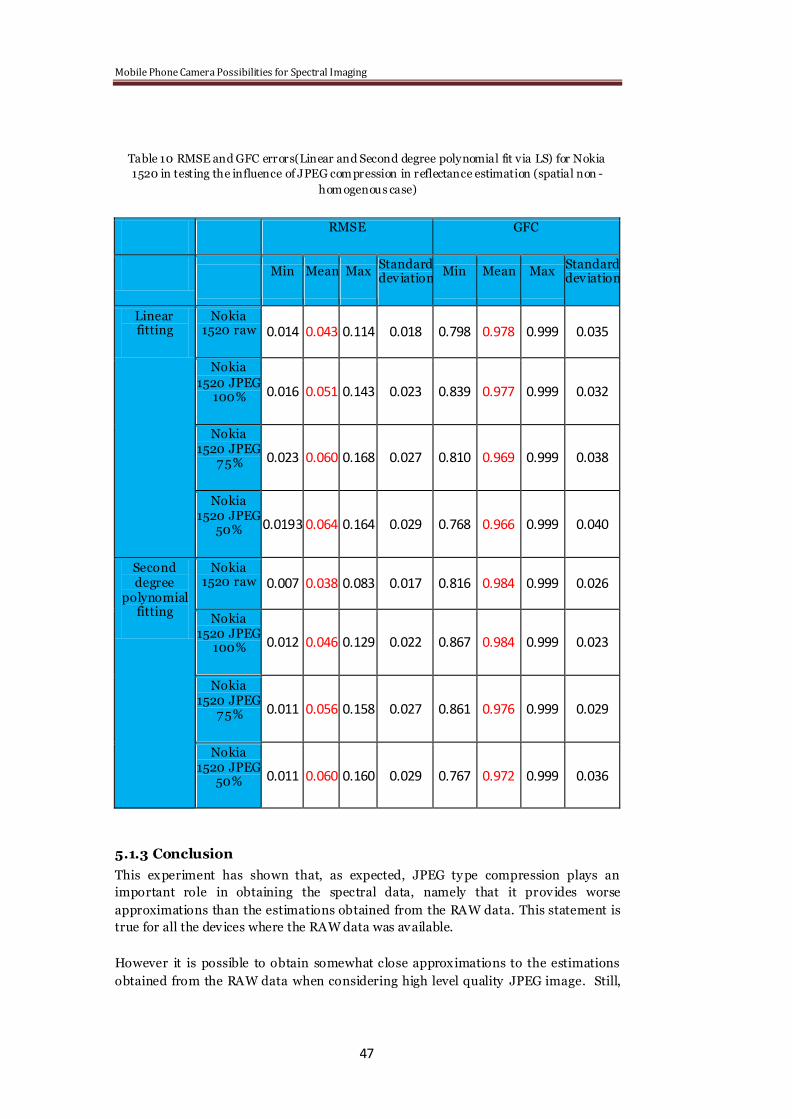
Mobile Phone Camera Possibilities for Spectral Imaging
47
Table 10 RMSE and GFC errors(Linear and Second degree polynomial fit via LS) for Nokia
1520 in testing the influence of JPEG compression in reflectance estimation (spatial non -
homogenous case)
RMSE GFC
Min Mean Max
Standard deviation
Min Mean Max Standard deviation
Linear fitting
Nokia 1520 raw 0.014 0.043 0.114 0.018 0.798 0.978 0.999 0.035
Nokia
1520 JPEG 100% 0.016 0.051 0.143 0.023 0.839 0.977 0.999 0.032
Nokia 1520 JPEG
75% 0.023 0.060 0.168 0.027 0.810 0.969 0.999 0.038
Nokia 1520 JPEG
50% 0.0193 0.064 0.164 0.029 0.768 0.966 0.999 0.040
Second degree
polynomial fitting
Nokia 1520 raw 0.007 0.038 0.083 0.017 0.816 0.984 0.999 0.026
Nokia 1520 JPEG
100% 0.012 0.046 0.129 0.022 0.867 0.984 0.999 0.023
Nokia 1520 JPEG
75% 0.011 0.056 0.158 0.027 0.861 0.976 0.999 0.029
Nokia 1520 JPEG
50% 0.011 0.060 0.160 0.029 0.767 0.972 0.999 0.036
5.1.3 Conclusion
This experiment has shown that, as expected, JPEG ty pe compression plays an
important role in obtaining the spectral data, namely that it provides worse
approximations than the estimations obtained from the RAW data. This statement is
true for all the dev ices where the RAW data was available.
However it is possible to obtain somewhat close approximations to the estimations
obtained from the RAW data when considering high level quality JPEG image. Still,

Mobile Phone Camera Possibilities for Spectral Imaging
48
special attention is needed when the imaged objects are not represented in a
homogenous type space, but as a real case scenario in which they contain high level of
detail.
5.2 Testing how the image processing block in digital image
affects reflectance estimation in smartphones
Another important step in investigating the value of the smartphone as a pocket
spectral imaging device was to test how the image processing block affects reflectance
estimation in comparison with the RAW images.
In order to test this we considered the JPEG and RAW images with the Xrite Color
Checker Digital SG taken with all the dev ices. The images were used further in
recovery of the spectral data. Again the estimation methods used were liniar fitting via
least squares and poly nomial fitting v ia least squares. The evaluation was anew LOO.
As we saw prev iously that compression plays an important role in spectral data
recovery, we tried eliminating these effects for the cases when JPEG ty pe data was
used. This was done by choosing the highest quality images that were possible to
obtain from the smartphones and digital cameras and also by considering for
estimation the case where the samples are spatially homogenous.
5.2.1 Liniar fitting via least squares
Results can be seen in Figure 27 and Tables 11, 12 for liniar fitting. Firstly we see from
Figure 27 that estimation errors obtained from JPEG are much higher than the ones
obtained from the RAW. Secondly we notice that estimating the reflectance from
RAW images provides the most stable results, as RMSE wavelength errors are closely
grouped together, while the ones obtained from the JPEG images vary considerably in
shape and intensity. Thirdly we see that from JPEG ty pe outputs the lowest error
comes from the Iphone device while the highest one comes from the Nikon D800
camera.
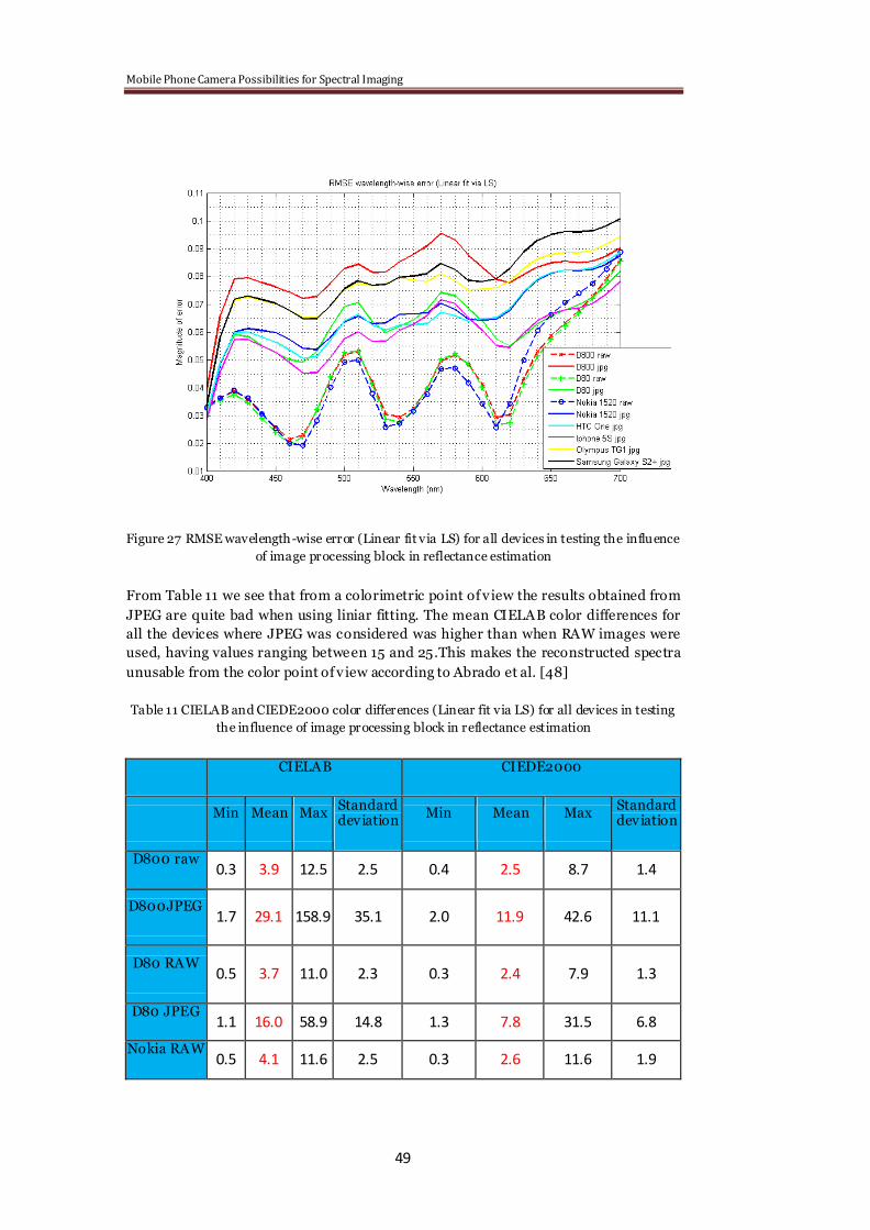
Mobile Phone Camera Possibilities for Spectral Imaging
49
Figure 27 RMSE wavelength-wise error (Linear fit via LS) for all devices in testing the influence
of image processing block in reflectance estimation
From Table 11 we see that from a colorimetric point of v iew the results obtained from
JPEG are quite bad when using liniar fitting. The mean CIELAB color differences for
all the devices where JPEG was considered was higher than when RAW images were
used, having values ranging between 15 and 25.This makes the reconstructed spectra
unusable from the color point of v iew according to Abrado et al. [48]
Table 11 CIELAB and CIEDE2000 color differences (Linear fit via LS) for all devices in testing
the influence of image processing block in reflectance estimation
CIELAB CIEDE2000
Min Mean Max Standard deviation
Min Mean Max Standard deviation
D800 raw 0.3 3.9 12.5 2.5 0.4 2.5 8.7 1.4
D800JPEG 1.7 29.1 158.9 35.1 2.0 11.9 42.6 11.1
D80 RAW 0.5 3.7 11.0 2.3 0.3 2.4 7.9 1.3
D80 JPEG 1.1 16.0 58.9 14.8 1.3 7.8 31.5 6.8
Nokia RAW 0.5 4.1 11.6 2.5 0.3 2.6 11.6 1.9
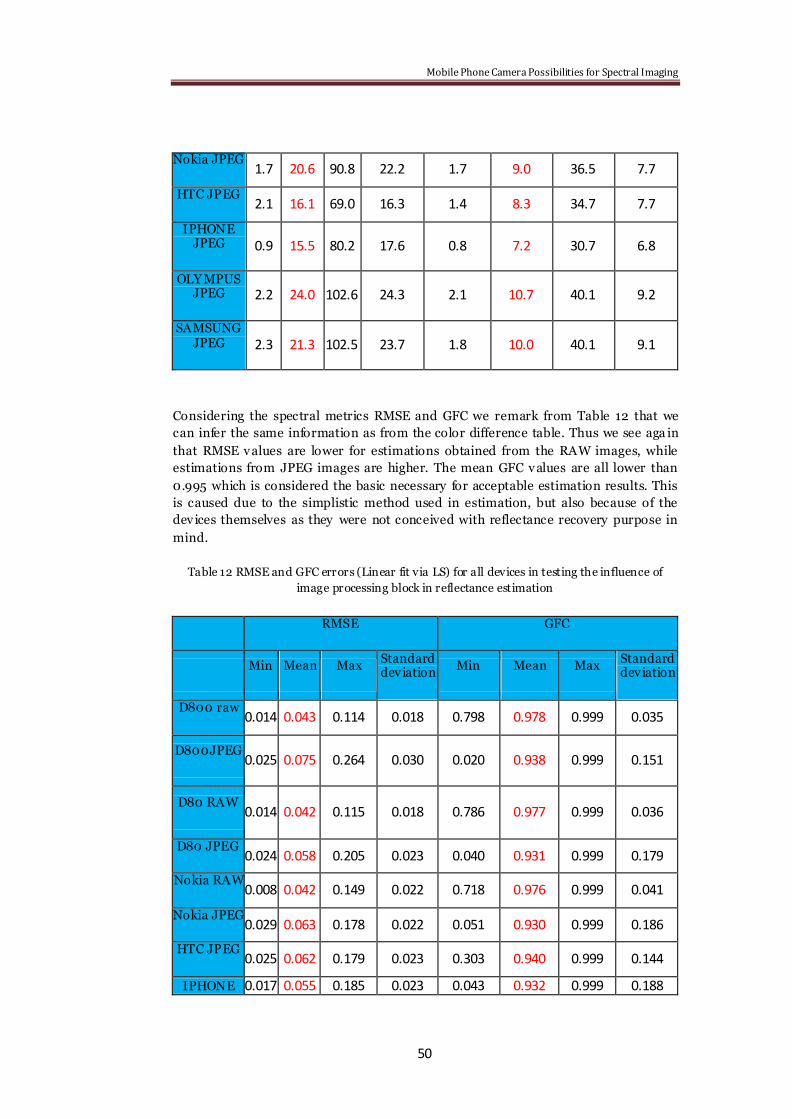
Mobile Phone Camera Possibilities for Spectral Imaging
50
Nokia JPEG 1.7 20.6 90.8 22.2 1.7 9.0 36.5 7.7
HTC JPEG 2.1 16.1 69.0 16.3 1.4 8.3 34.7 7.7
IPHONE JPEG 0.9 15.5 80.2 17.6 0.8 7.2 30.7 6.8
OLY MPUS JPEG 2.2 24.0 102.6 24.3 2.1 10.7 40.1 9.2
SAMSUNG JPEG 2.3 21.3 102.5 23.7 1.8 10.0 40.1 9.1
Considering the spectral metrics RMSE and GFC we remark from Table 12 that we
can infer the same information as from the color difference table. Thus we see aga in
that RMSE values are lower for estimations obtained from the RAW images, while
estimations from JPEG images are higher. The mean GFC values are all lower than
0.995 which is considered the basic necessary for acceptable estimation results. This
is caused due to the simplistic method used in estimation, but also because of the
dev ices themselves as they were not conceived with reflectance recovery purpose in
mind.
Table 12 RMSE and GFC errors (Linear fit via LS) for all devices in testing the influence of
image processing block in reflectance estimation
RMSE GFC
Min Mean Max Standard deviation
Min Mean Max Standard deviation
D800 raw 0.014 0.043 0.114 0.018 0.798 0.978 0.999 0.035
D800JPEG 0.025 0.075 0.264 0.030 0.020 0.938 0.999 0.151
D80 RAW 0.014 0.042 0.115 0.018 0.786 0.977 0.999 0.036
D80 JPEG 0.024 0.058 0.205 0.023 0.040 0.931 0.999 0.179
Nokia RAW 0.008 0.042 0.149 0.022 0.718 0.976 0.999 0.041
Nokia JPEG 0.029 0.063 0.178 0.022 0.051 0.930 0.999 0.186
HTC JPEG 0.025 0.062 0.179 0.023 0.303 0.940 0.999 0.144
IPHONE 0.017 0.055 0.185 0.023 0.043 0.932 0.999 0.188
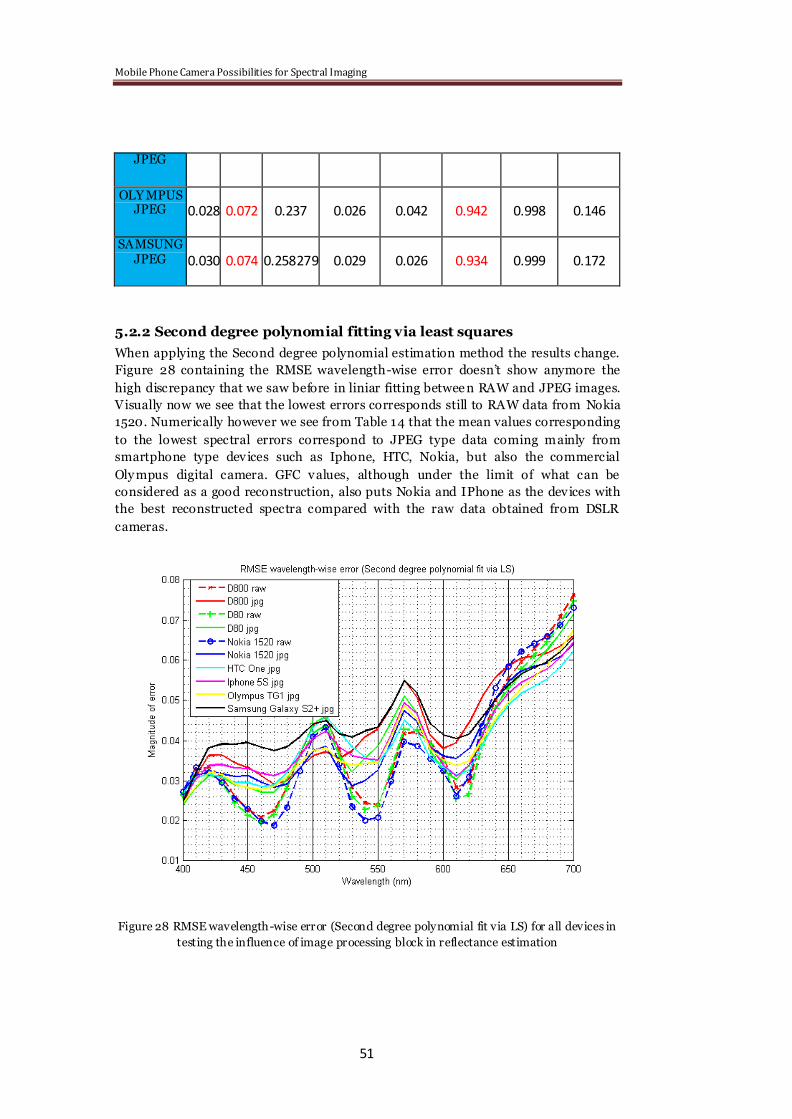
Mobile Phone Camera Possibilities for Spectral Imaging
51
JPEG
OLY MPUS JPEG 0.028 0.072 0.237 0.026 0.042 0.942 0.998 0.146
SAMSUNG JPEG 0.030 0.074 0.258279 0.029 0.026 0.934 0.999 0.172
5.2.2 Second degree polynomial fitting via least squares
When applying the Second degree polynomial estimation method the results change.
Figure 28 containing the RMSE wavelength-wise error doesn‘t show anymore the
high discrepancy that we saw before in liniar fitting betwee n RAW and JPEG images.
Visually now we see that the lowest errors corresponds still to RAW data from Nokia
1520. Numerically however we see from Table 14 that the mean values corresponding
to the lowest spectral errors correspond to JPEG type data coming mainly from
smartphone type dev ices such as Iphone, HTC, Nokia, but also the commercial
Oly mpus digital camera. GFC values, although under the limit of what can be
considered as a good reconstruction, also puts Nokia and IPhone as the dev ices with
the best reconstructed spectra compared with the raw data obtained from DSLR
cameras.
Figure 28 RMSE wavelength-wise error (Second degree polynomial fit via LS) for all devices in
testing the influence of image processing block in reflectance estimation
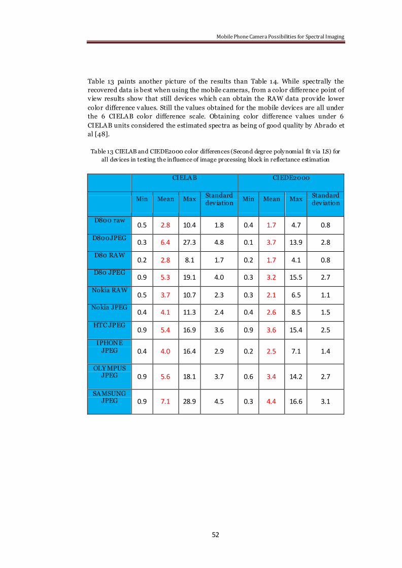
Mobile Phone Camera Possibilities for Spectral Imaging
52
Table 13 paints another picture of the results than Table 14. While spectrally the
recovered data is best when using the mobile cameras, from a color difference point of
v iew results show that still devices which can obtain the RAW data provide lower
color difference values. Still the values obtained for the mobile devices are all under
the 6 CIELAB color difference scale. Obtaining color difference values under 6
CIELAB units considered the estimated spectra as being of good quality by Abrado et
al [48].
Table 13 CIELAB and CIEDE2000 color differences (Second degree polynomial fit via LS) for
all devices in testing the influence of image processing block in reflectance estimation
CIELAB CIEDE2000
Min Mean Max Standard deviation
Min Mean Max Standard deviation
D800 raw 0.5 2.8 10.4 1.8 0.4 1.7 4.7 0.8
D800JPEG 0.3 6.4 27.3 4.8 0.1 3.7 13.9 2.8
D80 RAW 0.2 2.8 8.1 1.7 0.2 1.7 4.1 0.8
D80 JPEG 0.9 5.3 19.1 4.0 0.3 3.2 15.5 2.7
Nokia RAW 0.5 3.7 10.7 2.3 0.3 2.1 6.5 1.1
Nokia JPEG 0.4 4.1 11.3 2.4 0.4 2.6 8.5 1.5
HTC JPEG 0.9 5.4 16.9 3.6 0.9 3.6 15.4 2.5
IPHONE JPEG 0.4 4.0 16.4 2.9 0.2 2.5 7.1 1.4
OLY MPUS JPEG 0.9 5.6 18.1 3.7 0.6 3.4 14.2 2.7
SAMSUNG JPEG 0.9 7.1 28.9 4.5 0.3 4.4 16.6 3.1

Mobile Phone Camera Possibilities for Spectral Imaging
53
Table 14 RMSE and GFC errors (Second degree polynomial fit via LS) for all devices in testing
the influence of image processing block in reflectance estimation
RMSE GFC
Min Mean Max Standard deviation
Min Mean Max Standard deviation
D800 raw 0.007 0.038 0.083 0.017 0.815 0.984 0.999 0.026
D800JPEG 0.015 0.039 0.117 0.021 0.895 0.989 0.999 0.017
D80 RAW 0.007 0.037 0.083 0.016 0.816 0.984 0.999 0.027
D80 JPEG 0.009 0.037 0.115 0.020 0.851 0.986 0.999 0.025
Nokia RAW 0.007 0.036 0.119 0.018 0.771 0.984 0.999 0.029
Nokia JPEG 0.007 0.036 0.099 0.020 0.902 0.990 0.999 0.015
HTC JPEG 0.006 0.035 0.094 0.019 0.905 0.989 0.999 0.020
IPHONE JPEG 0.010 0.036 0.114 0.020 0.891 0.991 0.999 0.015
OLY MPUS JPEG 0.004 0.036 0.113 0.018 0.868 0.989 0.999 0.021
SAMSUNG JPEG 0.009 0.040 0.144 0.021 0.852 0.987 0.999 0.023
5.2.3 Conclusion
We saw in this test that even though we tried to reduce the effect of JPEG ty pe
compression, it still played an important role when testing the influence of the im age
processing block in reflectance estimation. This happened for all the dev ices
considered be they mobile cameras or DSLR cameras.
Another point that was seen here was that dependent on the estimation method used,
there is the possibility that under certain conditions, the estimation obtained from
smartphone cameras is better from a spectral point of v iew than the estimation
obtained from raw data of DSLR cameras. However colorimetric error values are still
higher. We noticed thus that the CIELAB errors are not statistically consistent with
the spectral errors. This is caused by the fact that we have a nonlinear transform from
the spectral reflectance to CIELAB values, thus the solution obtained as estimated
spectra is not optimal when evaluated by colorimetric error [27].
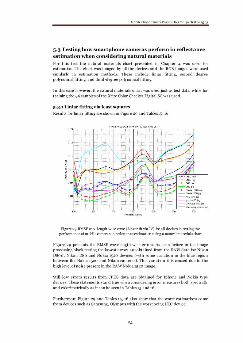
Mobile Phone Camera Possibilities for Spectral Imaging
54
5.3 Testing how smartphone cameras perform in reflectance
estimation when considering natural materials
For this test the natural materials chart presented in Chapter 4 was used for
estimation. The chart was imaged by all the devices and the RGB images were used
similarly in estimation methods. These include liniar fitting, second degree
polynomial fitting, and third-degree polynomial fitting.
In this case however, the natural materials chart was used just as test data, while for
training the 96 samples of the Xrite Color Checker Digital SG was used.
5.3.1 Liniar fitting via least squares
Results for liniar fitting are shown in Figure 29 and Tables15, 16.
Figure 29 RMSE wavelength-wise error (Linear fit via LS) for all devices in testing the
performance of mobile cameras in reflectance estimation using a natural materials chart
Figure 29 presents the RMSE wavelength-wise errors. As seen before in the image
processing block testing the lowest errors are obtained from the RAW data for Nikon
D800, Nikon D80 and Nokia 1520 devices (with some variation in the blue region
between the Nokia 1520 and Nikon cameras). This variation it is caused due to the
high level of noise present in the RAW Nokia 1520 image.
Still low errors results from JPEG data are obtained for Iphone and Nokia ty pe
dev ices. These statements stand true when considering error measures both spectrally
and colorimetrically as it can be seen in Tables 15 and 16.
Furthermore Figure 29 and Tables 15, 16 also show that the worst estimations come
from devices such as Samsung, Oly mpus with the worst being HTC device.
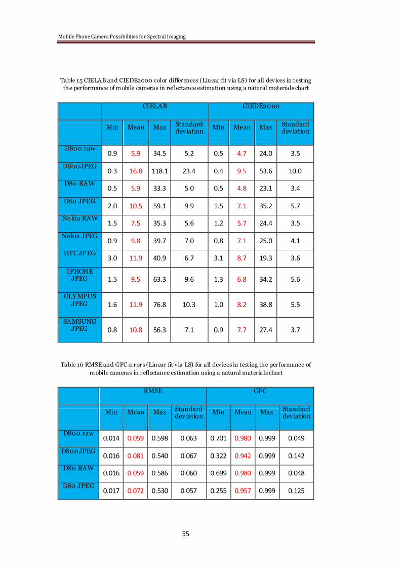
Mobile Phone Camera Possibilities for Spectral Imaging
55
Table 15 CIELAB and CIEDE2000 color differences (Linear fit via LS) for all devices in testing
the performance of mobile cameras in reflectance estimation using a natural materials chart
CIELAB CIEDE2000
Min Mean Max Standard deviation
Min Mean Max Standard deviation
D800 raw 0.9 5.9 34.5 5.2 0.5 4.7 24.0 3.5
D800JPEG 0.3 16.8 118.1 23.4 0.4 9.5 53.6 10.0
D80 RAW 0.5 5.9 33.3 5.0 0.5 4.8 23.1 3.4
D80 JPEG 2.0 10.5 59.1 9.9 1.5 7.1 35.2 5.7
Nokia RAW 1.5 7.5 35.3 5.6 1.2 5.7 24.4 3.5
Nokia JPEG 0.9 9.8 39.7 7.0 0.8 7.1 25.0 4.1
HTC JPEG 3.0 11.9 40.9 6.7 3.1 8.7 19.3 3.6
IPHONE JPEG 1.5 9.5 63.3 9.6 1.3 6.8 34.2 5.6
OLY MPUS JPEG 1.6 11.9 76.8 10.3 1.0 8.2 38.8 5.5
SAMSUNG JPEG 0.8 10.8 56.3 7.1 0.9 7.7 27.4 3.7
Table 16 RMSE and GFC errors (Linear fit via LS) for all devices in testing the performance of
mobile cameras in reflectance estimation using a natural materials chart
RMSE GFC
Min Mean Max Standard deviation
Min Mean Max Standard deviation
D800 raw 0.014 0.059 0.598 0.063 0.701 0.980 0.999 0.049
D800JPEG 0.016 0.081 0.540 0.067 0.322 0.942 0.999 0.142
D80 RAW 0.016 0.059 0.586 0.060 0.699 0.980 0.999 0.048
D80 JPEG 0.017 0.072 0.530 0.057 0.255 0.957 0.999 0.125
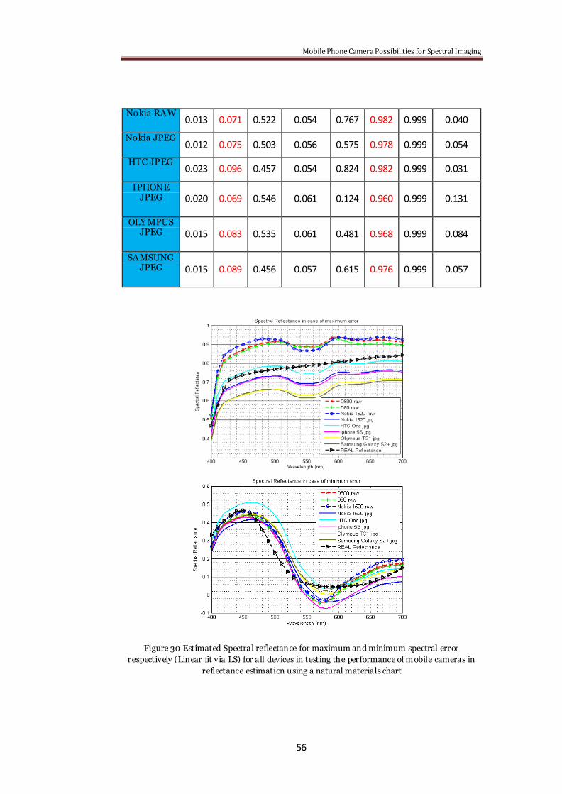
Mobile Phone Camera Possibilities for Spectral Imaging
56
Nokia RAW 0.013 0.071 0.522 0.054 0.767 0.982 0.999 0.040
Nokia JPEG 0.012 0.075 0.503 0.056 0.575 0.978 0.999 0.054
HTC JPEG 0.023 0.096 0.457 0.054 0.824 0.982 0.999 0.031
IPHONE JPEG 0.020 0.069 0.546 0.061 0.124 0.960 0.999 0.131
OLY MPUS JPEG 0.015 0.083 0.535 0.061 0.481 0.968 0.999 0.084
SAMSUNG JPEG 0.015 0.089 0.456 0.057 0.615 0.976 0.999 0.057
Figure 30 Estimated Spectral reflectance for maximum and minimum spectral error
respectively (Linear fit via LS) for all devices in testing the performance of mobile cameras in
reflectance estimation using a natural materials chart
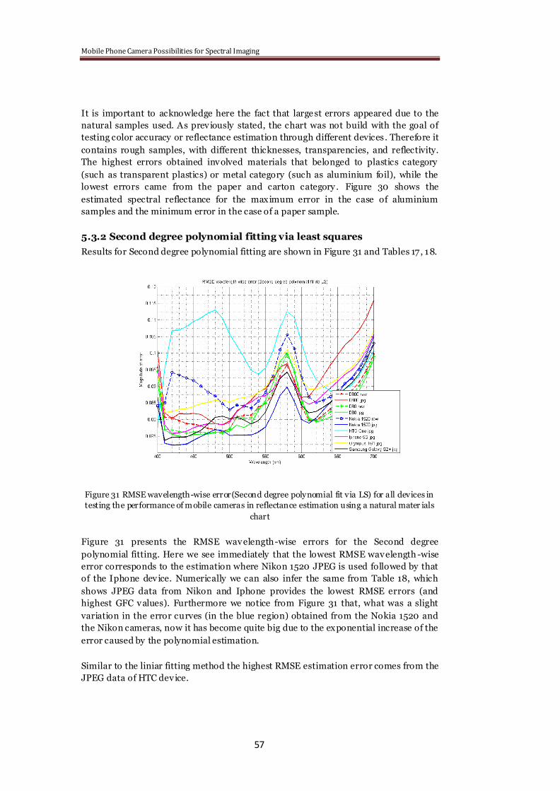
Mobile Phone Camera Possibilities for Spectral Imaging
57
It is important to acknowledge here the fact that largest errors appeared due to the
natural samples used. As prev iously stated, the chart was not build with the goal of
testing color accuracy or reflectance estimation through different devices . Therefore it
contains rough samples, with different thicknesses, transparencies, and reflectivity.
The highest errors obtained involved materials that belonged to plastics category
(such as transparent plastics) or metal category (such as aluminium foil), while the
lowest errors came from the paper and carton category . Figure 30 shows the
estimated spectral reflectance for the maximum error in the case of aluminium
samples and the minimum error in the case of a paper sample.
5.3.2 Second degree polynomial fitting via least squares
Results for Second degree polynomial fitting are shown in Figure 31 and Tables 17 , 18.
Figure 31 RMSE wavelength-wise error(Second degree polynomial fit via LS) for all devices in
testing the performance of mobile cameras in reflectance estimation using a natural mater ials
chart
Figure 31 presents the RMSE wavelength-wise errors for the Second degree
polynomial fitting. Here we see immediately that the lowest RMSE wavelength -wise
error corresponds to the estimation where Nikon 1520 JPEG is used followed by that
of the Iphone device. Numerically we can also infer the same from Table 18, which
shows JPEG data from Nikon and Iphone provides the lowest RMSE errors (and
highest GFC values). Furthermore we notice from Figure 31 that, what was a slight
variation in the error curves (in the blue region) obtained from the Nokia 1520 and
the Nikon cameras, now it has become quite big due to the exponential increase of the
error caused by the polynomial estimation.
Similar to the liniar fitting method the highest RMSE estimation error comes from the
JPEG data of HTC device.
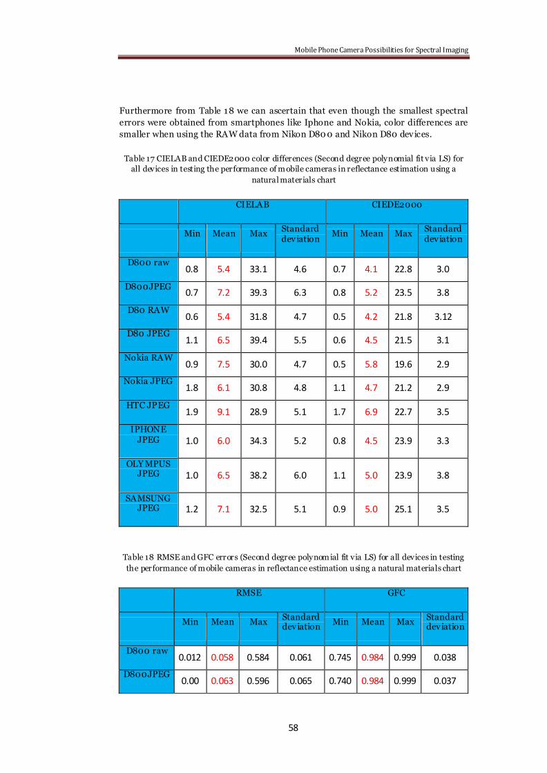
Mobile Phone Camera Possibilities for Spectral Imaging
58
Furthermore from Table 18 we can ascertain that even though the smallest spectral
errors were obtained from smartphones like Iphone and Nokia, color differences are
smaller when using the RAW data from Nikon D80 0 and Nikon D80 devices.
Table 17 CIELAB and CIEDE2000 color differences (Second degree polynomial fit via LS) for
all devices in testing the performance of mobile cameras in reflectance estimation using a
natural materials chart
CIELAB CIEDE2000
Min Mean Max Standard deviation
Min Mean Max Standard deviation
D800 raw 0.8 5.4 33.1 4.6 0.7 4.1 22.8 3.0
D800JPEG 0.7 7.2 39.3 6.3 0.8 5.2 23.5 3.8
D80 RAW 0.6 5.4 31.8 4.7 0.5 4.2 21.8 3.12
D80 JPEG 1.1 6.5 39.4 5.5 0.6 4.5 21.5 3.1
Nokia RAW 0.9 7.5 30.0 4.7 0.5 5.8 19.6 2.9
Nokia JPEG 1.8 6.1 30.8 4.8 1.1 4.7 21.2 2.9
HTC JPEG 1.9 9.1 28.9 5.1 1.7 6.9 22.7 3.5
IPHONE JPEG 1.0 6.0 34.3 5.2 0.8 4.5 23.9 3.3
OLY MPUS JPEG 1.0 6.5 38.2 6.0 1.1 5.0 23.9 3.8
SAMSUNG JPEG 1.2 7.1 32.5 5.1 0.9 5.0 25.1 3.5
Table 18 RMSE and GFC errors (Second degree polynomial fit via LS) for all devices in testing
the performance of mobile cameras in reflectance estimation using a natural materials chart
RMSE GFC
Min Mean Max Standard deviation
Min Mean Max Standard deviation
D800 raw 0.012 0.058 0.584 0.061 0.745 0.984 0.999 0.038
D800JPEG 0.00 0.063 0.596 0.065 0.740 0.984 0.999 0.037
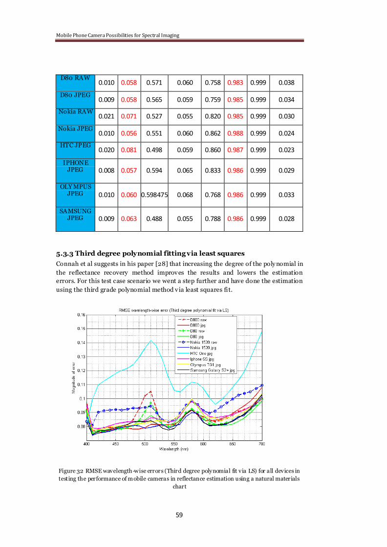
Mobile Phone Camera Possibilities for Spectral Imaging
59
D80 RAW 0.010 0.058 0.571 0.060 0.758 0.983 0.999 0.038
D80 JPEG 0.009 0.058 0.565 0.059 0.759 0.985 0.999 0.034
Nokia RAW 0.021 0.071 0.527 0.055 0.820 0.985 0.999 0.030
Nokia JPEG 0.010 0.056 0.551 0.060 0.862 0.988 0.999 0.024
HTC JPEG 0.020 0.081 0.498 0.059 0.860 0.987 0.999 0.023
IPHONE JPEG 0.008 0.057 0.594 0.065 0.833 0.986 0.999 0.029
OLY MPUS JPEG 0.010 0.060 0.598475 0.068 0.768 0.986 0.999 0.033
SAMSUNG JPEG 0.009 0.063 0.488 0.055 0.788 0.986 0.999 0.028
5.3.3 Third degree polynomial fitting via least squares
Connah et al suggests in his paper [28] that increasing the degree of the poly nomial in
the reflectance recovery method improves the results and lowers the estimation
errors. For this test case scenario we went a step further and have done the estimation
using the third grade polynomial method v ia least squares fit.
Figure 32 RMSE wavelength-wise errors (Third degree polynomial fit via LS) for all devices in
testing the performance of mobile cameras in reflectance estimation using a natural materials
chart
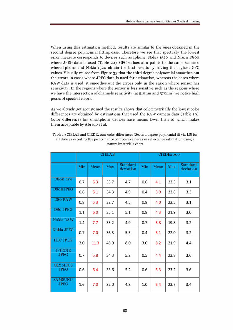
Mobile Phone Camera Possibilities for Spectral Imaging
60
When using this estimation method, results are similar to the ones obtained in the
second degree polynomial fitting case. Therefore we see that spectrally the lowest
error measure corresponds to devices such as Iphone, Nokia 1520 and Nikon D800
where JPEG data is used (Table 20). GFC values also points to the same scenario
where Iphone and Nokia 1520 obtain the best results by having the highest GFC
values. Visually we see from Figure 33 that the third degree polynomial smoothes out
the errors in cases where JPEG data is used for estimation, whereas the cases where
RAW data is used, it smoothes out the errors only in the region where sensor has
sensitiv ity . In the regions where the sensor is less sensitive such as the regions where
we have the intersection of channels sensitivity (at 510nm and 570nm) we notice high
peaks of spectral errors.
As we already got accustomed the results shows that colorimetrically the lowest color
differences are obtained by estimations that used the RAW camera data (Table 19).
Color differences for smartphone devices have means lower than 10 which makes
them acceptable by Abrado et al.
Table 19 CIELAB and CIEDE2000 color differences (Second degree polynomial fit via LS) for
all devices in testing the performance of mobile cameras in reflectance estimation using a
natural materials chart
CIELAB CIEDE2000
Min Mean Max Standard deviation
Min Mean Max Standard deviation
D800 raw 0.7 5.3 33.7 4.7 0.6 4.1 23.3 3.1
D800JPEG 0.6 5.1 34.3 4.9 0.4 3.9 23.8 3.3
D80 RAW 0.8 5.3 32.7 4.5 0.8 4.0 22.5 3.1
D80 JPEG 1.1 6.0 35.1 5.1 0.8 4.3 21.9 3.0
Nokia RAW 1.4 7.7 33.2 4.9 0.7 5.8 19.8 3.2
Nokia JPEG 0.7 7.0 36.3 5.5 0.4 5.1 22.0 3.2
HTC JPEG 3.0 11.3 45.9 8.0 3.0 8.2 21.9 4.4
IPHONE JPEG 0.7 5.8 34.3 5.2 0.5 4.4 23.8 3.6
OLY MPUS JPEG 0.6 6.4 33.6 5.2 0.6 5.3 23.2 3.6
SAMSUNG JPEG 1.6 7.0 32.0 4.8 1.0 5.4 23.7 3.4
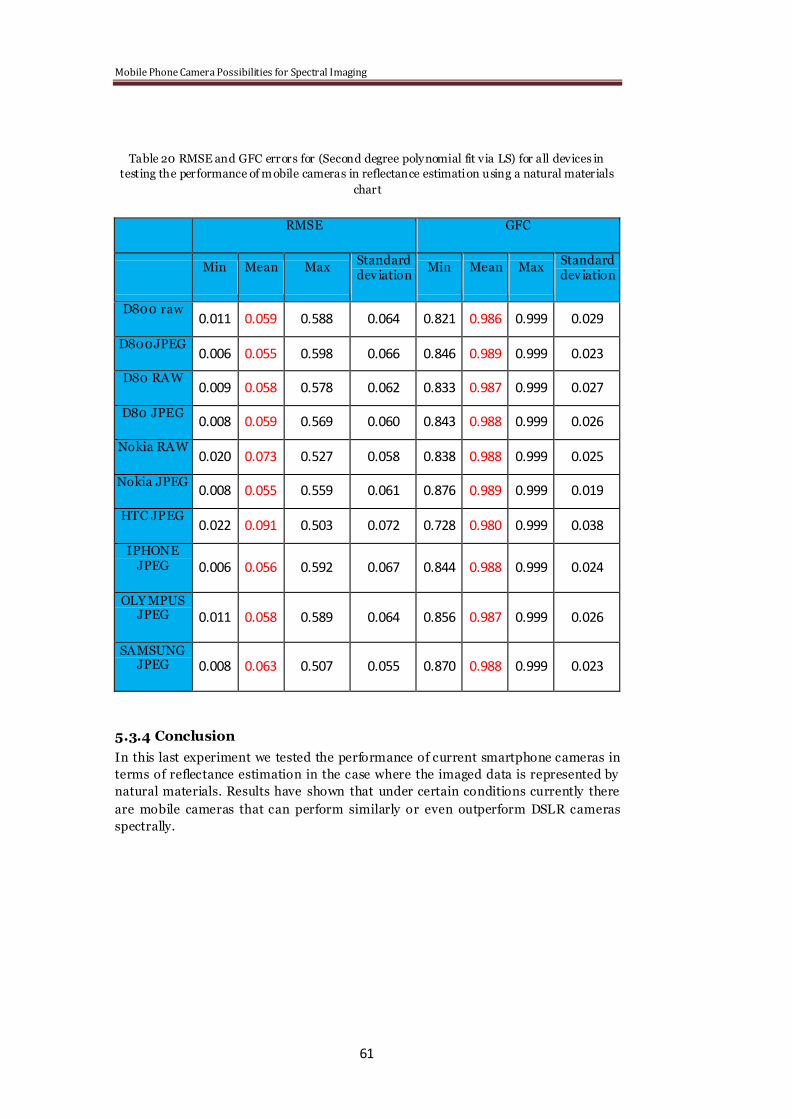
Mobile Phone Camera Possibilities for Spectral Imaging
61
Table 20 RMSE and GFC errors for (Second degree polynomial fit via LS) for all devices in
testing the performance of mobile cameras in reflectance estimation using a natural materials
chart
RMSE GFC
Min Mean Max Standard deviation
Min Mean Max Standard deviation
D800 raw 0.011 0.059 0.588 0.064 0.821 0.986 0.999 0.029
D800JPEG 0.006 0.055 0.598 0.066 0.846 0.989 0.999 0.023
D80 RAW 0.009 0.058 0.578 0.062 0.833 0.987 0.999 0.027
D80 JPEG 0.008 0.059 0.569 0.060 0.843 0.988 0.999 0.026
Nokia RAW 0.020 0.073 0.527 0.058 0.838 0.988 0.999 0.025
Nokia JPEG 0.008 0.055 0.559 0.061 0.876 0.989 0.999 0.019
HTC JPEG 0.022 0.091 0.503 0.072 0.728 0.980 0.999 0.038
IPHONE JPEG 0.006 0.056 0.592 0.067 0.844 0.988 0.999 0.024
OLY MPUS JPEG 0.011 0.058 0.589 0.064 0.856 0.987 0.999 0.026
SAMSUNG JPEG 0.008 0.063 0.507 0.055 0.870 0.988 0.999 0.023
5.3.4 Conclusion
In this last experiment we tested the performance of current smartphone cameras in
terms of reflectance estimation in the case where the imaged data is represented by
natural materials. Results have shown that under certain conditions currently there
are mobile cameras that can perform similarly or even outperform DSLR cameras
spectrally.

Mobile Phone Camera Possibilities for Spectral Imaging
62

Mobile Phone Camera Possibilities for Spectral Imaging
63
6 Conclusions and Future Work
In this work we focused on study ing the practicality and usefulness of smartphones
and their cameras as a single standing spectral imaging device. The study in the thesis
is structured as a comparison between smart-phone cameras and DSLR cameras as
their digital output in the form of RAW (obtained mainly from the DSLR came ras)
and JPEG ty pe data provide an important role in obtaining the spectral estimation of
the imaged objects. Several test cases were made in order to see the problems that
arise when considering smartphone devices as spectral imaging devices. Upon
recovering the spectral data diffrent reflectance estimation methods were
implemented such as the liniar fitting v ia least square and multivariate poly nomial
fitting v ia least squares. Also evaluation of the estimation methods were realized by
implementing different spectral and colorimetric metrics such as RMSE, GFC and
RMSE wavelength-wise, CIELAB and CIEDE2000 color differences.
The problems considered were how the JPEG type compression algorithm and also
how the image processing block influences reflectance recovery . This experiment has
shown that, as expected, JPEG ty pe compression plays an important role in obtaining
the spectral data, namely that it provides worse estimations with increasing level of
compression than the estimations obtained from the RAW data. However under the
tested conditions it is possible to obtain somewhat close reflectance estimations (to
the ones obtained from the RAW data) when considering using high level quality
JPEG image. Similarly it was found that the image processing block play s also quite
an important role influencing a great deal the estimation. Results showed that even
though smartphone cameras have similar ty pe of sensors recovery accuracy varies
greatly between devices.
Also performance of current smartphone cameras in terms of reflectance estimation
was tested in the case where the imaged data is represented by natural materials.
Results have shown that under certain conditions, currently there are mobile cameras
such as Nokia 1520 and Iphone 5S that can offer spectral recovery similarly to DSLR
cameras even with JPEG ty pe formats. However RAW data from DSLRs offers more
―stable‖ results colorimetrically. This statistical inconsistency is caused by the fact
that we have a nonlinear transform from the spectral reflectance to CIELAB values,
thus the solution obtained as estimated spectra is not optimal when evaluated by
colorimetric error.
Another aspect found when trying to use the smartphone as a spectral imaging device
is that it emplies the usage of certain estimation models. This is due to the inability of
the user to have access to the sensitiv ities of the sensor (due to company policies, and
inability to capture RAW data), which represents much needed information in many
recovery methods. Thus we have a limitation of the estimation models that can be
employed.
Future work involves testing the reflectance recovery when using as tr aining, charts
with more color samples. It is widely known in literature that increasing the number

Mobile Phone Camera Possibilities for Spectral Imaging
64
of training samples the accuracy in spectral recovery will be greater improved. Also it
would be interesting to see what is the minimum number of training samples in order
to obtain good spectral data from the smartphones. Also as future work it is needed to
see how different illumination and estimation methods affects the results obtained so
far.
Even more the final goal is to create custom software application which includes
reduced and adapted image processing in order provide analytical measurements of a
spectral image. This can be used in a broad range of fields such as it will allow a
novice user to use applications that carry out analysis on objects that require spectral
information mobile imaging in artworks, cultural heritage, medical imaging, pattern
recognition (automated photo editing) etc.
Mobile Phone Camera Possibilities for Spectral Imaging
65
Bibliography
[1] Koskinen I.K., 2007, Mobile Multimedia in Action, by Transaction Publishers,
New Brunswick, New Jersey.
[2] Kindberg, T., Spasojev ic, M., Fleck, R. & Sellen, A., 2005, The ubiquitous camera:
an in-depth study of camera phone use ‘, in IEEE Pervasive Computing, vol. 4, no. 2,
Apr.– Jun.
[3] Gye L. 2007, Picture This: The Impact of Mobile Camera Phones on Personal
Photographic Practices, published in Continuum Vol 21 Issue 2. pp 279-288
[4] Slavuj R., Green P., To develop a method for estimating spectral reflectance from
camera RGB values, The Norwegian Color and Visual Computing Laboratory , Gjøvik,
Norway
[5] Hardeberg J. Y., Schmitt F., and Brettel. H., 2002, Multispectral color image
capture using a liquid crystal tunable filter. Optical Engineering, 41
[6] Berns R. S., Taplin L. A., Nezamabadi M., Mohammadi M., and Zhao Y., 2005,
Spectral imaging using a commercial colorfilter array digital camera . In 14th
Triennal ICOM-CC meeting, pages 743–750
[7 ] Hyvarinen T., Herrala E., Dall‘Ava A., 1998, Direct sight imaging spectrograph: a
unique add-on component brings spectral imaging to industrial applications, Proc.
SPIE
[8] Hirai A., Hashimoto M., Itoh K. and Ichioba Y., 1997, Multichannel spectral
imaging system for measurement with high signal-to-noise ratio , Optical Review 4,
334-341
[9] Heikkinen V., Mirhashemi A., Alho J., 2013, Link functions and Matérn kernel in
the estimation of reflectance spectra from RGB responses, J. Opt. Soc. Am. A / Vol.
30, No. 11 / November 2013
[10] Jiang J., Gu J., 2012, Recovering Spectral Reflectance under commonly lighting
conditions, Computer Vision and Pattern Recognition Workshops (CVPRW)
[11] Imai F., Berns R. S., and Tzeng D., 2000, A comparative analysis of spectral
reflectance estimation in various spaces using a trichromatic camera system, J.
Imaging Sci. Technol. 44, 280–287
[12] Gebejes A., Martinez Domingo M. A., Heikkinen V., Tomic I., Sept 2013,
Reflectance recovery for coated printed color samples via multiangular RGB
camera measurements, , Color and Visual Computing Sy mposium
Mobile Phone Camera Possibilities for Spectral Imaging
66
[13] Miy a., Miyata K, 1999, Color Image Processing Based on Spectral Information
and Its Application, Image Processing, ICIP 99. Proceedings
[14] Stigell P., Miy ata K., Hauta-Kasari M., 2007 , Wiener Estimation Method in
Estimating of Spectral Reflectance from RGB Images, ISSN 1054-6618, Pattern
Recognition and Image Analysis, 2007, Vol. 17 , No. 2, pp. 233 –242. © Pleiades
Publishing, Ltd.,
[15] Hae Song J., Kim C., Yoo Y., March 2014, Vein Visualization using a Smart
Phone with Multispectral Wiener Estimation for Point-of-Care Applications,
published in Biomedical and Health Informatics, IEEE Journal of (Volume:PP ,
Issue: 99 ),
[16] Ohta N. and Robertson A. R., 2005, Colorimetry. Fundamentals and
Applications, John Wiley & Sons, Ltd
[17] Fairchild M. D., Rosen M. R., Johnson G. M., Spectral and Metameric Color
Imaging Technical Report, Munsell Color Science Laboratory
[18] Gebejes A., Tomic I., Karlovic I. and Juric I., 2012, Evaluation of the algorithms
for recovering spectral reflectance from virtual digital camera response , Journal of
Graphic Engineering and Design
[19] Electro Magnetic Spectrum, [Online]. Available:
http://www.pion.cz/en/article/electromagnetic -spectrum
[20] Digital Camera Signal Processing Flow, [Online]. Available:
http://panasonic.jp/support/global/cs/dsc/knowhow/knowhow30.html
[21] Huang B-C., Fuh C-S., 2005, Image Pipeline Algorithms for Standard Mobile
Imaging Architecture Sensors, 18th IPPR Conference on Computer Vision, Graphics
and Image Processing (CVGIP 2005)
[22] Chen T., 2003, Digital Camera System Simulator and Applications , Phd Thesis
[23] Nakamura J., 2006, Image Sensors and Signal Processing for Digital Still
Cameras, published by CRC press, Taylor & Francis Group
[24] Zhou P., 2007, Getting the Most out of Your Image-Processing Pipeline , white
paper of Texas Instruments Incorporated
[25] Lebourgeois V., Begue A., Labbe S., Mallavan B., Prevot L. and Roux B. , 2008,
Can Commercial Digital Cameras Be Used as Multispectral Sensors? A Crop
Monitoring Test, Sensors, 8, 7300-7322; DOI: 10.3390/s8117300
[26] Shimano N., Terai K., Hironaga M., October 2007, Recovery of spectral
reflectances of objects being imaged by multispectral cameras , Vol. 24, No.10,
Journal Opt. Soc. Am. A

Mobile Phone Camera Possibilities for Spectral Imaging
67
[27] Zhang W.F., Dai D.Q., September 2008, Spectral reflectance estimation from
camera responses by support vector regression and a composite model , J. Opt. Soc.
Am , A/Vol. 25, No. 9/ Sept. 2008
[28] Connah D., Hardeberg J. Y., 2005, Spectral recovery using polynomial models,
Proc. SPIE 5667, 65-75
[29] Heikkinen V., Lenz R., Jestsu T., Parkkinen J., Hauta-Kasari M., Jaaskelainen T.,
October 2008, Evaluation and unification of some methods for estimating
reflectance spectra from RGB images, J. Opt. Soc. Am. A/Vol. 25, No. 10/
[30]Heikkinen V., Jestu T., Parkkinen J., Hauta-Kasari M., Jaaskelainen T. and Lee S.
D., 2007, Regularized learning framework in the estimation of reflectance spectra
from camera responses, J. Opt. Soc. Am. A 24, 2673-2683
[31] Hardeberg J. Y, 2004, Filter selection for multispectral color image acquisition,
J. Imaging Sci. Technol., 48, 105 -110
[32] Nieves J. L., Valero E. M., Nascimento S. M. C., Andres J. H., and Romero J.,
2005, Multispectral synthesis of daylight using a commercial digital CCD camera,
Appl . Opt., 44, 5696-5703
[33] Jetsu T., Heikkinen V., Parkkinen J., Hauta-Kasari M., Martinkauppi B., Lee S.
D., Ok H. W. and Kim C. Y ., 2006, Color calibration of digital camera using
polynomial transformation, in CGIV, Third European Conference on Color Graphics,
Imaging and Vision (IS&T,), 163-166
[34] Haneishi H., Hasegawa T., Hosoi A., Yokoyama Y., Tsumura N. and Miy ake Y.,
2000, System design for accurately estimating the reflectance spectra of art
paintings, Appl. Opt., 39, 6621-6623 ()
[35] Hernandez-Andres J., Romero J., Garcıa-Beltran A., and Nieves J.L., 1998,
Testing linear models on spectral daylight measurements, Appl. Opt. 37 , 971–977
[36] Romero J., Garcıa-Beltran A., and Hernandez-Andres J., 1997, Linear bases for
representation of natural and artificial illuminants , J. Opt. Soc. Am. A 14, 1007 –
1014
[37] Hernandez-Andres J., Romero J. and Nieves J.L., 2001, Color and spectral
analysis of daylight in southern Europe , Vol. 18, No. 6/June 2001/ J. Opt. Soc. Am.
A
[38] Imai F.H., Rosen M.R. and Berns R.S. 2002, Comparative Study of Metrics for
Spectral Match Quality, CGIV 2002: The First European Conference on Colour
Graphics, Imaging, and Vision
[39] Viggiano, J A Stephen, Metrics for evaluating spectral matches: a quantitative
comparison. Proceedings of CGIV -2004: the Second European Conference on Colour
Mobile Phone Camera Possibilities for Spectral Imaging
68
Graphics, Imaging, and Vision. Springfield, VA: IS&T — The Society for Imaging
Science & Technology, 2004, in press.
[40] Lopez-Alvarez M.A., Hernandez-Andres J., Valero E.M. and Nieves J.L.,
Colorimetric and Spectral Combined Metric for the Optimization of Multispectral
Systems , AIC Colour 05 - 10th Congress of the International Colour Association
[41] Connah D., Hardeberg J. Y ., 2004, Comparison of linear spectral reconstruction
methods for multispectral imaging, Internation Conference of Image Processing
(ICIP 2004)
[42] Xrite Color Checker Digital SG, [Online]. Available:
http://xritephoto.com/ph_product_overv iew.aspx?id=938
[43] Specim Imspector V10E datasheet [Online]. Available:
http://www.specim.fi/files/pdf/core/datasheets/VIS-VNIR-ImSpectors-ver1-
2011.pdf
[44] Specim Imspector V10E photo. [Online]. Available:
http://www.aelab.co.za/images/stories/specim/imaging_spectograph/vis_vnir/vnir/
vnir1.jpg
[45] Shimano N., July 2006, Recovery of Spectral Reflectances of Objects Being
Imaged Without Prior Knowledge, IEEE Transactions on Image Processing, Vol.15,
No.7 , July 2006
[46] Imai F. H., Berns R. S., 1999, Spectral Estimation Using Trichromatic Digital
Cameras, Proceedings of the International Sy mposium on Multispectral Imaging and
Color Reproduction for Digital Archives (Society of Multispectral Imaging of Japan,
Chiba University , Japan, 1999)
[47] Komiya Y., Ohsawa K., Obi T., Yamaguchi M., Ohy ama N., 1999, Natural Color
Reproduction System for Telemedicine and Its Application to Digigal Camera, Proc
IEEE, 50 54 (1999)
[48] Abrardo A., Alparone L., Cappellini V., Prosperi A., 1999, Color Constancy fom
Multispectral Images, Proc. IEEE 570, 574 (1999)
[49] Hardeberg J. Y., 1999, Acquisition and reproduction of colour images:
colorimetric and multispectral approaches, PhD Thesis (Ecole Nationale Superieure
des Telecommunications, Departament TSI, Paris, France, 1999)
[50] Quijano Ruiz J. I, September 2010, Quality metrics for spectral estimation,
Master thesis in Photonics, registered at Escola Tecnica Superior D‘Enginyeria de
Telecomunicacio de Barcelona.
[51] Wy szecki G, Color Science: concepts and methods, quantitative data and
formulae, (John Wiley & Sons, New York, 1982).

Mobile Phone Camera Possibilities for Spectral Imaging
69
[52] CIE Publication 142, Improvement to Industrial Colour-Difference Evaluation,
Commission Internationale de L‘Éclairage, (V ienna, Austria, 2001).
[53] Bayer E. B.,1 976, Color imaging array, U.S. Patent No. 3,971,065
[54] Antikainen J, 2012, New Techniques for Spectral Image Acquisition and
Analysis, PhD thesis, Publications of the University of Eastern Finland Dissertations
in Forestry and Natural Sciences, No 73
[55] Jetsu T., Hertzog P., Jaaskelainen T. and Parkkinen J., 2005, Standardization of
spectral Image Formats, Pattern recognition and Image analy sis, 15, 618-620
[56] Hauta-Kasari M., Lehtonen J., Parkkinen J., and Jääskeläinen T., Image Format
for Spectral Image Browsing, IS & T Journal of Imaging Science and Technology 50
(2006).
[57] Swain P.K. Cheskis D., Back-Illuminated Image Sensors Come to the Forefront
[Online], Available: http://www.photonics.com/Article.aspx?AID=34685
[58] Sony develops back-illuminated CMOS image sensor [Online], Available:
http://www.sony.net/SonyInfo/News/Press/200806/08-069E/index.html
[59] BSI (Backside Illumination) [Online], Available:
http://www.semicon.toshiba.co.jp/eng/product/sensor/cmos/bsi/index.html
[60] Cardinal D., How back-illuminated sensors work, and why they’re the future of
digital photography [Online], Available:
http://www.extremetech.com/extreme/149742-how-back-illuminated-sensors-work-
and-why-theyre-the-future-of-digital-photography
[61] An Objective Look at FSI and BSI , An AptinaTM Technology White Paper
[Online], Available: http://www.aptina.com/news/FSI-BSI-WhitePaper.pdf
[62] Spectral Image data cube [Online], Available:
http://zeiss.magnet.fsu.edu/tutorials/spectralimaging/lambdastack/lambdastacktuto
rialfigure1.jpg
[63] Peterson C., How It Works: The Charged-Coupled Device, or CCD [Online],
Available: http://www.if.ufrgs.br/~marcia/ccd.pdf
[64] Buried channel charge coupled devices, US Patent US 3792322 A, [Online],
Available: http://www.google.com./patents/US3792322
[65] Tay lor S. A., CCD and CMOS Imaging Array Technologies: Technology Review,
Technical Report EPC-1998-106, Xerox Research Centre Europe, 1998, [Online],
Available: http://research.microsoft.com/pubs/80353/ccd.pdf
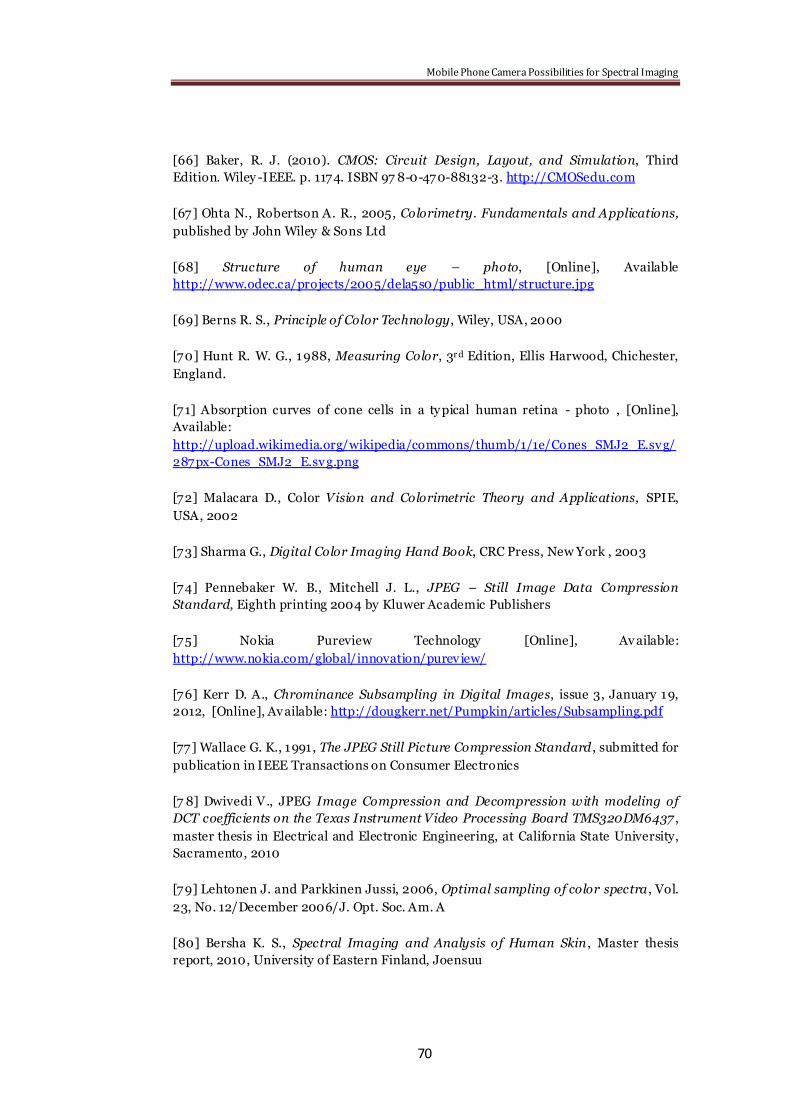
Mobile Phone Camera Possibilities for Spectral Imaging
70
[66] Baker, R. J. (2010). CMOS: Circuit Design, Layout, and Simulation, Third
Edition. Wiley -IEEE. p. 1174. ISBN 97 8-0-470-88132-3. http://CMOSedu.com
[67] Ohta N., Robertson A. R., 2005, Colorimetry. Fundamentals and Applications,
published by John Wiley & Sons Ltd
[68] Structure of human eye – photo, [Online], Available
http://www.odec.ca/projects/2005/dela5s0/public_html/structure.jpg
[69] Berns R. S., Principle of Color Technology, Wiley, USA, 2000
[70] Hunt R. W. G., 1988, Measuring Color, 3r d Edition, Ellis Harwood, Chichester,
England.
[71] Absorption curves of cone cells in a ty pical human retina - photo , [Online],
Available:
http://upload.wikimedia.org/wikipedia/commons/thumb/1/1e/Cones_SMJ2_E.svg/
287px-Cones_SMJ2_E.svg.png
[72] Malacara D., Color Vision and Colorimetric Theory and Applications, SPIE,
USA, 2002
[73] Sharma G., Digital Color Imaging Hand Book, CRC Press, New York , 2003
[74] Pennebaker W. B., Mitchell J. L., JPEG – Still Image Data Compression
Standard, Eighth printing 2004 by Kluwer Academic Publishers
[75] Nokia Pureview Technology [Online], Av ailable:
http://www.nokia.com/global/innovation/pureview/
[76] Kerr D. A., Chrominance Subsampling in Digital Images, issue 3, January 19,
2012, [Online], Available: http://dougkerr.net/Pumpkin/articles/Subsampling.pdf
[77] Wallace G. K., 1991, The JPEG Still Picture Compression Standard , submitted for
publication in IEEE Transactions on Consumer Electronics
[7 8] Dwivedi V., JPEG Image Compression and Decompression with modeling of
DCT coefficients on the Texas Instrument Video Processing Board TMS320DM6437 ,
master thesis in Electrical and Electronic Engineering, at California State University,
Sacramento, 2010
[79] Lehtonen J. and Parkkinen Jussi, 2006, Optimal sampling of color spectra , Vol.
23, No. 12/December 2006/J. Opt. Soc. Am. A
[80] Bersha K. S., Spectral Imaging and Analysis of Human Skin , Master thesis
report, 2010, University of Eastern Finland, Joensuu
http://upload.wikimedia.org/wikipedia/commons/thumb/1/1e/Cones_SMJ2_E.svg/287px-Cones_SMJ2_E.svg.png

Mobile Phone Camera Possibilities for Spectral Imaging
71
[81] Hauta Kasari M., 1999, Computational Techniques for Spectral Image Analysis,
PhD thesis, Lappeenranta Univeristy of Technology, Lappeenranta , Finland
[82] Penczek J., Boyton P. A. and Splett J.D., Color Error in Digital Camera Image
Capture Process, J Digit Imaging (2014) 27:182–191
[83] Eriksson M. and Iqbal Z., Two measurement modes for mobile phone optical
sensing, 2014, Sensors and actuators. B, Chemical, (195), 63-70. Available:
http://dx.doi.org/10.1016/j.snb.2014.01.005
[84] Garcia A., Erenas M.M., Marinetto E. D., Abad C. A., de Orbe-Paya I., Palma A. J.
and Capitan-Vallvey L. F., Mobile Phone Platform as portable chemical analyzer.,
Elsev ier , Sensors and Actuators B 156 (2011) 350 –359
[85] Iqbal Z., Bjorklund R.B., Assesment of a mobile phone for use as a spectroscopic
analytical tool for foods and beverages, International Journal of Food Science and
Technology 2011, 46, 2428–2436
[86] Iqbal Z., Filippini D., Spectral Fingerprinting on a Standard Mobile Phone ,
Hindawi Publishing Corporation, Journal of Sensors, Volume 2010, Article ID
381796, 9 pages doi:10.1155/2010/381796
[87 ] Alakarhu J., Image Sensors and Image Quality in Mobile Phones, Nokia,
Technology Platforms, Camera Entity
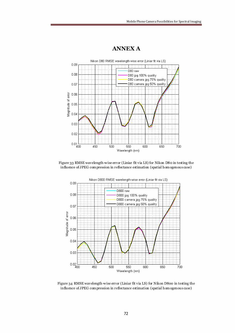
Mobile Phone Camera Possibilities for Spectral Imaging
72
ANNEX A
Figure 33 RMSE wavelength-wise error (Liniar fit via LS) for Nikon D80 in testing the
influence of JPEG compression in reflectance estimation (spatial homogenous case)
Figure 34 RMSE wavelength-wise error (Liniar fit via LS) for Nikon D800 in testing the
influence of JPEG compression in reflectance estimation (spatial homogenous case)
Mobile Phone Camera Possibilities for Spectral Imaging
73
Table 21 CIELAB and CIEDE2000 color difference (Liniar fit via LS) for Nikon D800 in testing
the influence of JPEG compression in reflectance estimation (spatial homogenous case)
CIELAB CIEDE2000
Min Mean Max Standard deviation
Min Mean Max Standard deviation
D80 raw 0.5 3.7 11.0 2.3 0.3 2.4 7.9 1.3
D80 JPEG 100%
0.3 3.7 11.3 2.3 0.5 2.4 8.3 1.3
D80 JPEG 75%
0.5 4.3 12.7 2.6 0.4 2.7 8.9 1.6
D80 JPEG 50%
0.7 4.1 14.0 2.9 0.6 2.5 12.5 1.5
D800raw 0.3 3.9 12.5 2.5 0.4 2.5 8.7 1.4
D800JPEG 100%
0.5 4.1 13.3 2.6 0.6 2.6 8.9 1.6
D800 JPEG 75%
0.8 4.4 13.0 2.8 0.5 2.9 11.6 2.0
D800 JPEG 50%
0.7 4.9 23.5 3.8 0.4 3.1 16.3 2.7
Table 22 RMSE and GFC errors (Liniar fit via LS) for Nikon D800 in testing the influence of
JPEG compression in reflectance estimation (spatial homogenous case)
RMSE GFC
Min Mean Max Standard deviation
Min Mean Max Standard deviation
D80 raw 0.014 0.042 0.115 0.018 0.786 0.977 0.999 0.036
D80 JPEG 100% 0.013 0.042 0.117 0.018 0.781 0.977 0.999 0.037
D80 JPEG 75% 0.014 0.042 0.120 0.019 0.792 0.977 0.999 0.037
D80 JPEG 50% 0.015 0.043 0.114 0.018 0.768 0.976 0.999 0.039

Mobile Phone Camera Possibilities for Spectral Imaging
74
D800 raw 0.014 0.043 0.114 0.018 0.798 0.978 0.999 0.035
D800 JPEG 100% 0.013 0.043 0.114 0.018 0.799 0.978 0.999 0.034
D800 JPEG 75% 0.015 0.043 0.113 0.018 0.796 0.978 0.999 0.035
D800 JPEG 50% 0.008 0.043 0.119 0.019 0.799 0.977 0.999 0.035

Mobile Phone Camera Possibilities for Spectral Imaging
75
ANNEX B
Figure 35 RMSE wavelength-wise error (Second degree polynomial fit via LS) for Nikon D80in
testing the influence of JPEG compression in reflectance estimation (spatial homogenous case)
Figure 36 RMSE wavelength-wise error (Second degree polynomial fit via LS) for Nikon D800
in testing the influence of JPEG compression in reflectance estimation (spatial homogenous
case)
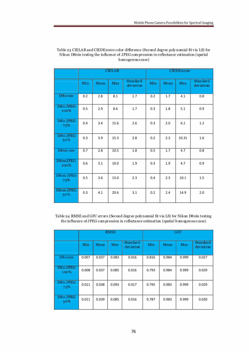
Mobile Phone Camera Possibilities for Spectral Imaging
76
Table 23 CIELAB and CIEDE2000 color difference (Second degree polynomial fit via LS) for
Nikon D80in testing the influence of JPEG compression in reflectance estimation (spatial
homogenous case)
CIELAB CIEDE2000
Min Mean Max Standard deviation
Min Mean Max Standard deviation
D80 raw 0.2 2.8 8.1 1.7 0.2 1.7 4.1 0.8
D80 JPEG 100%
0.5 2.9 8.6 1.7 0.3 1.8 5.1 0.9
D80 JPEG 75%
0.4 3.4 15.6 2.6 0.3 2.0 6.1 1.2
D80 JPEG 50%
0.3 3.9 15.3 2.8 0.2 2.3 10.31 1.6
D800 raw 0.7 2.8 10.5 1.8 0.5 1.7 4.7 0.8
D800JPEG 100%
0.6 3.1 10.0 1.9 0.3 1.9 4.7 0.9
D800 JPEG 75%
0.5 3.6 13.0 2.3 0.4 2.3 10.1 1.5
D800 JPEG 50%
0.3 4.1 20.6 3.1 0.2 2.4 14.9 2.0
Table 24 RMSE and GFC errors (Second degree polynomial fit via LS) for Nikon D80in testing
the influence of JPEG compression in reflectance estimation (spatial homogenous case)
RMSE GFC
Min Mean Max Standard deviation
Min Mean Max Standard deviation
D80 raw 0.007 0.037 0.083 0.016 0.816 0.984 0.999 0.027
D80 JPEG 100%
0.008 0.037 0.085 0.016 0.793 0.984 0.999 0.029
D80 JPEG 75%
0.011 0.038 0.093 0.017 0.795 0.983 0.999 0.029
D80 JPEG 50%
0.011 0.039 0.085 0.016 0.787 0.983 0.999 0.030

Mobile Phone Camera Possibilities for Spectral Imaging
77
D800 raw 0.007 0.038 0.083 0.017 0.816 0.984 0.999 0.026
D800 JPEG 100%
0.008 0.038 0.083 0.017 0.807 0.984 0.999 0.027
D800 JPEG 75%
0.007 0.038 0.081 0.017 0.819 0.985 0.999 0.026
D800 JPEG 50%
0.009 0.038 0.089 0.018 0.798 0.983 0.999 0.030