These probabilities can be represented by a transition proba-bility matrix M . Both the rows and columns of M are indexedby length-k strings from Ak so that P (Xn+1 = a|X(1, n) =L(1, n)) = M(s, s′) where s = L(n − k + 1, n), the currentcontext, and and s′ = L(n−k+2, n)a, the next context. In thatcase, knowing M would immediately provide the probabilityfor each possible next symbol of L.

Since we do not know M , we can generate an estimateP̂ from the current history L, the current context c, and theequation

P̂ (Xn+1 = a|L) =N(ca, L)N(c, L)

(1)

where N(s′, s) denotes the number of times the substring s′

occurs in the string s.Given this estimate, we can easily define the behavior of the

O(k) Markov predictor. It predicts the symbol a ∈ A with themaximum probability P̂ (Xn+1 = a|L), that is, the symbolthat most frequently followed the current context c in prioroccurrences in the history. Notice that if c has never occurredbefore, the above equation evaluates to 0/1 = 0 for all a, andthe O(k) Markov predictor makes no prediction.

If the location history is not generated by an order-k Markovsource, then this predictor is, of course, only an approximation.

Fortunately, O(k) Markov predictors are easy to implement.Our implementation maintains an estimate of the (sparse)matrix M , using Equation 1. To make a prediction, thepredictor scans the row of M corresponding to the currentcontext c, choosing the entry with the highest probability for itsprediction. After the next move occurs, the predictor updatesthe appropriate entry in that row of M , and updates c, inpreparation for the next prediction.

Vitter and Krishnan [9] use O(k) predictors to prefetch diskpages, and prove interesting asymptotic properties of thesepredictors. Other variations of Markov predictors can be foundin the survey [7].

LZ familyLZ-based predictors are based on a popular incremental

parsing algorithm by Ziv and Lempel [10] often used for textcompression. This approach seems promising because (a) mostgood text compressors are good predictors [9] and (b) LZ-based predictors are like the O(k) Markov predictor exceptthat k is a variable allowed to grow to infinity [5]. We brieflydiscuss how the LZ algorithm works.

Let γ be the empty string. Given an input string s, the LZparsing algorithm partitions the string into distinct substringss0, s1, . . . , sm such that s0 = γ, and for all j > 0 substringsj without its last character is equal to some si, 0 ≤ i < j,and s0s1 . . . sm = s. Observe that the partitioning is donesequentially, i.e., after determining each si the algorithmonly considers the remainder of the input string. Using theexample from Figure 1, s = gbdcbgcefbdbde is parsed asγ, g, b, d, c, bg, ce, f, bd, bde.

Associated with the algorithm is a tree, the LZ tree, that isgrown dynamically during the parsing process. Each node of

γ

g:1b:4

d:1c:2

f:1

g:1 e:1

s = gbdcbgcefbdbdesi = γ, g, b, d, c, bg, ce, f, bd, bde

d:2

e:1

Figure 2. Example LZ parsing tree

the tree represents one substring si. The root is labeled γ andthe other nodes are labeled with a symbol from A so that thesequence of symbols encountered on the path from the rootto that node forms the substring associated with that node.Since this LZ tree is to be used for prediction, it is necessaryto store some statistics at each node. The tree resulting fromparsing the above example is shown in Figure 2; each node islabeled with its location symbol and the value of its statistic,a counter, after parsing.

To parse a (sub)string s we trace a path through the LZ tree.If any child of the current node (initially the root) matches thefirst symbol of s, remove that symbol from s and step down tothat child, incrementing its counter; continue from that node,examining the next symbol from s. If the symbol did not matchany child of the current node, then remove that symbol froms and add a new child to the current node, labeled with thatsymbol and counter=1; resume parsing at the root, with thenow shorter string s.

Based on the LZ parsing algorithm, several predictors havebeen suggested in the past [9], [11], [12], [5], [6]. We describesome of these below and then discuss how they differ. Formore detailed information, please refer to [7].

LZ predictors. Vitter and Krishnan [9] considered the casewhen the generator of L is a finite-state Markov source, whichproduces sequences where the next symbol is dependent ononly its current state. (We note that a finite-state Markovsource is different from the O(k) Markov source in that thestates do not have to correspond to strings of a fixed lengthfrom A.) They suggested estimating the probability, for eacha ∈ A, as

P̂ (Xn+1 = a|L) =NLZ(sma, L)NLZ(sm, L)

(2)

Copyright IEEE INFOCOM 2004 3

where NLZ(s′, s) denotes the number of times s′ occurs as aprefix among the substrings s0, . . . , sm which were obtainedby parsing s using the LZ algorithm.

It is worthwhile comparing Equation (1) with Equation (2).While the former considers how often the string of interestoccurs in the entire input string, the latter considers how oftenit occurs in the partitions si created by LZ. Thus, in theexample of Figure 2, while dc occurs in L it does not occurin any si.

The LZ predictor chooses the symbol a in A that hasthe highest probability estimate, that is, the highest value ofP̂ (Xn+1 = a|L). An on-line implementation need only buildthe LZ tree as it parses the string, maintaining node countersas described above. After parsing the current symbol thealgorithm rests at a node in the tree. It examines the childrenof the current node, if any, and predicts the symbol labelingthe child with the highest counter, which indicates the highestfrequency of past occurrence. If the current node is a leaf, theLZ predictor makes no prediction.

LZ-Prefix and PPM.Bhattacharya and Das propose a heuristic modification to

the construction of the LZ tree [5], as well as a way of usingthe modified tree to predict the most likely cells that containthe user so as to minimize paging costs to locate that user.

As we mention above, not every substring in L forms a nodesi in the LZ parsing tree. In particular, substrings that crossboundaries of the si, 0 < i ≤ m, are missed. Further, previousLZ-based predictors take into account only the occurrencestatistics for the prefixes of the leaves. To overcome this,they proposed the following modification. When a new leafis created for si, all the proper suffixes of si (i.e., all thesuffixes not including si itself) are also inserted into the tree.If a node representing a suffix does not exist, it is created;and the occurrence counter for every prefix of every suffix isincremented.

Example. Suppose the current leaf is sm = bde and thestring de is one that crosses boundaries of existing si for1 ≤ i < m. Thus de has not occurred as a prefix or a suffixof any si, 0 < i < m. The set of proper suffixes of sm isSm = {γ, e, de}, and since there is no node representing thesubstring for de, it is created. Then the occurrence frequencyis incremented for the root labeled γ, the first-level children band d, and the new leaf node de. Figure 3 shows the tree afterthis transformation, which we call “LZ+prefix” or “LZP” forshort.

We observe that this heuristic only discovers substringsthat lie within a leaf string. Nonetheless, at this point it ispossible to use the modified LZ tree and apply one of theexisting prediction heuristics, e.g., use Eq. 2 and the Vitter-Krishnan method. Indeed, we include the LZP predictor in ourcomparison.

Bhattacharya and Das [5] propose a further heuristic thatuses the LZP tree for prediction. This second heuristic isbased on the Prediction by Partial Match (PPM) algorithmfor text compression [13]. (The PPM algorithm essentially

γ

g:2b:4

d:3c:2

f:1

g:1 e:1

s = gbdcbgcefbdbdesi = γ, g, b, d, c, bg, e, ce, f, bd, de, bde

d:2

e:1

e:1

e:2

Figure 3. Example LZP parsing tree

attempts to “blend” the predictions of several O(k) Markovpredictors; we do not describe it here in detail.) Given aleaf string sm, construct its set of proper suffixes Sm andupdate the LZP tree as described above. Then, for each suchsuffix, the heuristic considers the subtree rooted at the suffixand finds all the paths in this subtree originating from thissubtree root. The PPM algorithm is then applied to this set ofpaths. PPM first computes the predicted probability of eachpath, and then uses these probabilities to compute the mostprobable next symbol(s) based on their weights (number ofoccurrences) in the path. We include the “LZ+prefix+PPM”predictor, nicknamed “LeZi” [5], in our comparison.

C. Breaking ties

In our descriptions of the predictors, above, we indicatethat each predicts the symbol with the highest probability ofoccurring next, given the current state of its data structure(Markov matrix or LZ tree). It is quite possible, though, forthere to be a tie for first place, that is, several symbols withequal probability and none with higher probability. None of theliterature indicates how to break a tie, yet our implementationsmust make a specific choice. We implemented 3 different tie-break methods:

• First added: among the symbols that tie, we predict thefirst one added to the data structure, that is, the first oneseen in the location history.

• Most recently added: among the symbols that tie, wepredict the one that was most recently added to the datastructure.

• Most recent: among the symbols that tie, we predict theone most recently seen in the history.

In Figure 4, we show the ratio of the number of ties and thenumber of predictions, using a cumulative distribution function(CDF) across all users having more than 1000 movements fordifferent predictors (the O(2) Markov fallback predictor willbe described later). Fortunately, Figure 4 shows that most ofthe users had few ties, less than about 10% of all predictions.

Copyright IEEE INFOCOM 2004 4

0

0.2

0.4

0.6

0.8

1

0 0.2 0.4 0.6 0.8 1

Fra

ctio

n of

use

rs

Ratio of number of ties and number of predictions

O(1) MarkovO(2) Markov fallback

LZLZP

Figure 4. Ratio of number of ties and the number of predictions

Our experiments showed that the results were not significantlyaffected by the choice of a tie-breaking method. We used the“first added” method throughout the results below, and do notconsider tie-breakers further.

D. Entropy metric

We believe that there are some intrinsic characteristics ofa trace that ultimately determine its predictability and hencethe performance of different predictors. In the results section,we compare the accuracy metric with the entropy metric, foreach user, on several predictors.

In general, the entropy H(X) of a discrete random variableX is defined as

H(X) = −∑x∈X

P (x) log2 P (x) (3)

where X is the set of all possible of values of x.In this paper, we compute the entropy of a given user under

the O(k) Markov predictor. We obtain the probabilities P (x)from the data structures constructed by that predictor on thatuser’s trace.

If C is the set containing all the context strings encounteredin parsing a location history L, then the conditional entropyis

H(X|C) = −∑c∈C

N(c, L)n − k + 1

∑a∈A

P (x = a|c) log2 P (x = a|c)(4)

E. Accuracy metric

During an on-line scan of the location history, the predictoris given a chance to predict each location. There are threepossible outcomes for this prediction, when compared to theactual location:

• The predictor correctly identified the location of the nextmove.

• The predictor incorrectly identified the location of thenext move.

• The predictor returned “no prediction.”

All predictors encounter situations in which they are unableto make a prediction; in particular, all realistic predictors willhave no prediction for the first location of each user trace.

We define the accuracy of a predictor for a particular userto be the fraction of locations for which the predictor correctlyidentified the next move. Thus, “no prediction” is counted asan incorrect prediction. In the future we plan to examine othermetrics that can better distinguish the two forms of incorrectprediction (there may be some applications that may prefer noprediction to a wild guess). For now, this metric best reflectsthe design of predictors common in the literature.

F. Data collection

We have been monitoring usage on the Wi-Fi network atDartmouth College since installation began in April 2001.Installation was largely complete by June 2001, and as ofMarch 2003 there are 543 access points providing 11 Mbpscoverage to the entire campus. Although there was no specificeffort to cover outdoor spaces, the campus is compact and theinterior APs tend to cover most outdoor spaces. The wirelesspopulation is growing fast. As of May 2003 there are between2,500 and 3,500 users active in any given day.

The access points transmit a “syslog” message every timea client card associated, re-associated, or disassociated; themessage contains the unique MAC address of the client card.Although a given card might be used in multiple devices or adevice used by multiple people, in this paper we think of thewireless card as a “network user” and thus the term “user”refers to a wireless card.

We have a nearly continuous, two-year record of thesesyslog messages from April 2001 through March 2003. Ourdata has some brief “holes” when the campus experienced apower failure, or when a central syslog daemon apparentlyhung up. Also, since syslog uses UDP it is possible that somemessages were lost or misordered. In March 2002, we installedtwo redundant servers to record the data, so that holes in oneof the servers can be filled by the data recorded by the otherserver.

For more information about Dartmouth’s network and ourdata collection, see our previous study [14] [15].

After we cleaned the data of some glitches, and mergedthe data from two servers (where available), we extracted usertraces from the data. Each user’s trace is a series of locations,that is, access-point names. We introduced the special location“OFF” to represent the user’s departure from the network(which occurs when the user turns off their computer or theirwireless card, or moves out of range of all access points).The traces varied widely in length (number of locations in thesequence), with a median of 494 and a maximum of 188,479;most are shown in Figure 5. Users with longer traces wereeither more active (using their card more), more mobile (thuschanging access points more often), or used the network fora longer period (some users have been on the network since

Copyright IEEE INFOCOM 2004 5

0

0.2

0.4

0.6

0.8

1

0 500 1000 1500 2000 2500 3000 3500 4000 4500 5000

Fra

ctio

n of

use

rs

Trace length

Figure 5. Length of user traces

April 2001, and some others have only recently arrived oncampus).

G. Evaluation experiments

To evaluate a predictor, we run each user’s trace indepen-dently through our implementation of that predictor. For eachlocation in the trace, the predictor updates its data structureand then makes a prediction about the next location. Ourexperiments framework tracks the accuracy of the predictor.

III. RESULTS

We evaluated the location predictors using our Wi-Fi mo-bility data. In this section we examine the results.

A. Markov

Recall that accuracy is defined as the number of correctpredictions divided by the number of attempts (moves). Aswe step through the locations in a single trace, attemptingto predict each location in sequence, we can examine theaccuracy up to that point in the trace. Figure 6 shows how theaccuracy metric varies over the course of one user’s history,using the O(1) Markov predictor. Ultimately, for comparisonpurposes, we define the accuracy over the entire trace, therightmost value in this plot. In subsequent graphs we use thisoverall accuracy as the performance metric.

Of course, we have several thousand users and the predictorwas more successful on some traces than on others. In Figure 7we display the accuracy of the O(1) Markov predictor inCDF curves, one for each of three groups of traces: short,medium, and long traces. It is obvious that curves “to theright” are better, because for a given fraction of users, theright curve has a higher prediction accuracy. The predictorwas clearly unsuccessful on most short traces (100 or fewermoves), because its curve is far to the left. Ultimately, wefound that all predictors fared poorly on traces with fewer than1000 moves, and we restrict the remainder of our comparison

0

0.2

0.4

0.6

0.8

1

0 500 1000 1500 2000 2500 3000 3500 4000 4500 5000

Acc

urac

y

Position in location history

O(1) Markov

Figure 6. Prediction accuracy for a sample user

0

0.2

0.4

0.6

0.8

1

0 0.2 0.4 0.6 0.8 1

Fra

ctio

n of

use

rs

Accuracy

O(1) Markov (1000+ moves) median=0.64O(1) Markov (100-1000 moves) median=0.57

O(1) Markov (<=100 moves) median=0.28

Figure 7. Accuracy of O(1) Markov predictor

to traces of more than 1000 moves. There were 2,195 suchusers, out of 6,202 total users traced.

After such strong evidence that the predictor’s accuracy wasbetter, in general, for users with longer traces, it is tempting tosuggest that accuracy is somewhat correlated with trace length.Figure 8 also shows there is a slight trend that longer traceshave higher prediction accuracy, although it is not a lineardependence.

Intuitively, it should help to use more context in eachattempt to predict the next location. In Figure 9 we comparethe accuracy of O(1) Markov with that of O(2), O(3), andO(4) Markov predictors. As an aside, we include an “order0” Markov predictor, in which no context is used in the pre-diction of each move. This predictor simply predicts the mostfrequent location seen so far in that user’s history. Althoughit represents a degenerate form of Markov prediction, it helpsto show the benefit of context in the O(1) predictor.

Copyright IEEE INFOCOM 2004 6

0

0.2

0.4

0.6

0.8

1

0 2000 4000 6000 8000 10000

Acc

urac

y

Length

O(1) Markov

Figure 8. Correlating accuracy with trace length

0

0.2

0.4

0.6

0.8

1

0 0.2 0.4 0.6 0.8 1

Fra

ctio

n of

use

rs

Accuracy

O(0) Markov median=0.35O(1) Markov median=0.64O(2) Markov median=0.70O(3) Markov median=0.67O(4) Markov median=0.63

Figure 9. Comparing Markov predictors

Not surprisingly, O(2) generally outpredicted O(1), and itscurve is further to the right. The high-order O(3) and O(4)predictors were, however, worse than O(2). Although thesepredictors use more information in the prediction process, theyare also more likely to encounter a context (a three- or four-location string) that has not been seen before, and thus beunable to make a prediction. A missing prediction is not acorrect prediction, and these unpredicted moves bring downthe accuracy of the higher-order predictors. In Figure 10 wedisplay the conditional accuracy of these same predictors:the number of correct predictions divided by the number ofpredictions. In this metric, we ignore unpredicted moves, andit becomes clear that longer context strings did lead to betterprediction, where possible, although with diminishing returns.

Returning to our original accuracy metric, we now con-sider a meta-predictor based on the Markov predictor family.Figure 11 displays the performance of the O(2) Markov

0

0.2

0.4

0.6

0.8

1

0 0.2 0.4 0.6 0.8 1

Fra

ctio

n of

use

rs

Conditional Accuracy

O(1) Markov conditional median=0.66O(2) Markov conditional median=0.75O(3) Markov conditional median=0.77O(4) Markov conditional median=0.78

Figure 10. Conditional accuracy metric

0

0.2

0.4

0.6

0.8

1

0 0.2 0.4 0.6 0.8 1

Fra

ctio

n of

use

rs

Accuracy

O(1) Markov median=0.64O(2) Markov median=0.70

O(2) Markov fallback median=0.72

Figure 11. Markov predictors with fallback

predictor with “fallback,” which used the results of the O(2)predictor when it made a prediction, or the O(1) predictor ifthe O(2) predictor had no prediction. In general, the O(k)fallback predictor recursively used the result of the O(k − 1)predictor (with k = 0 as the base of the recursion) whenever itencountered an unknown context. Fallback indeed helped toimprove the O(2) Markov predictor’s performance. O(3) andO(4) Markov also improved with fallback, but the results arenearly identical to the O(2) Markov with fallback and are thusnot shown. Markov predictors with fallback gain the advantageof the deeper context but without losing accuracy by failingto predict in unknown situations.

In the plots so far we examine the performance of O(k)Markov predictors that used the most recent k locations inmaking a prediction, weighting the potential next locations bytheir frequency of occurrence in the past. An alternative ap-proach assigns weights according to the recency of occurrence

Copyright IEEE INFOCOM 2004 7

0

0.2

0.4

0.6

0.8

1

0 0.2 0.4 0.6 0.8 1

Fra

ctio

n of

use

rs

Accuracy

O(1) Markov Recent. median=0.68O(2) Markov Recent. median=0.65

O(2) Markov Recent. fallback median=0.66

Figure 12. Markov using “most recent”

in the past; thus, one transition (the most recent seen for thiscontext) has weight 1 and the others have weight 0. Observethat the Order-k Markov prediction using the most-frequentlocation in general takes O(nk+1) space, while using themost-recent location it takes only O(nk) space, a potentiallysignificant decrease in storage. Figure 12 shows the qualityof Markov predictors based on this approach. Curiously, hereO(2) did worse than O(1), although fallback made up someof the difference. We are still exploring the reason behind thiscurious difference.

In Figure 13 we compare the recency-weighted approachwith the original frequency-weighted approach. The bestrecency-weighted Markov predictor, O(1), was better thanthe corresponding frequency-weighted predictor. This resultimplies that recent history was a better predictor of theimmediate future than was an accumulated probability model,when considering only the current location. On the otherhand, recall from Figure 12 that among the recency-weightedpredictors the extra context of O(2) lowered prediction ac-curacy. Thus, among O(2) predictors, the frequency-weightedapproach beats the recency-weighted approach (not shown inFigure 13). Ultimately, the O(2) frequency-weighted Markovpredictor with fallback has the best outcome.

Some of our user traces span a period of hours or days,but some span weeks or months. Clearly it is possible fora user’s mobility patterns to change over time; for example,a student may move to a new dormitory, or attend differentclasses. The transition weights constructed by the frequency-weighted Markov model may become ineffective after such achange; for users with a long history, these weights will adapttoo slowly. In another series of experiments (not shown), weadded an exponential decay to the frequency weights so thatmore recent locations have a larger impact, but we saw littleimprovement in the quality of the predictors. We need to studythis option further.

0

0.2

0.4

0.6

0.8

1

0 0.2 0.4 0.6 0.8 1

Fra

ctio

n of

use

rs

Accuracy

O(1) Markov Freq. median=0.64O(1) Markov Recent median =0.68

O(2) Markov Freq. fallback median=0.72

Figure 13. Markov: “most recent” vs. “most frequent”

B. LZ-based

We first consider the LZ predictor, shown in Figure 14.Since LZ makes no prediction whenever the current contextstring leads to a leaf in the tree, the plot includes two LZvariants. As an alternative to no prediction (the first curve),we can use the statistics at the root (second curve) to makea prediction based on the probability of each location. Thatis, when the predictor encounters a leaf, it behaves as if it isat the root and simply predicts the most frequently seen childof the root. Given our accuracy metric, it is always betterto make some prediction than no prediction, and indeed inthis case the accuracy improved significantly. An even betterapproach (third curve) is to fallback to progressively shortersubstrings of the current context, much as we did with theMarkov predictors, until a substring leads to a non-leaf nodefrom which we can make a prediction. This fallback abilityis critical to allow prediction to occur while the tree grows,since the trace often leads to a leaf just before adding a newleaf.

Later, Bhattacharya and Das [5] proposed two extensions tothe LZ predictor. Figure 15 displays the performance of thefirst extension, LZP. Once again, this predictor (as defined)makes no prediction when the context leads to a leaf, and onceagain it helped to use statistics at the root, or (better) fallback.The second extension produces a LZ+prefix+PPM predictornicknamed “LeZi.” Figure 16 compares the performance of LZwith LZP and LeZi, showing that each extension did improvethe accuracy of the LZ predictor substantially.

When we compare the best variant of each LZ form, inFigure 17, it becomes clear that the simple addition of ourfallback technique to the LZ predictor did just as well asthe prefix and PPM extensions combined. (LeZi automaticallyincludes fallback by adding suffix substrings into the tree,so there is no fallback variant.) LZ with fallback is a muchsimpler predictor than LZP or LeZi, and since the accuracyis similar (and as we show below, the LZ data structure was

Copyright IEEE INFOCOM 2004 8

0

0.2

0.4

0.6

0.8

1

0 0.2 0.4 0.6 0.8 1

Fra

ctio

n of

use

rs

Accuracy

LZ no-predict at leaf median=0.53LZ use root stat. at leaf median=0.61

LZ fallback at leaf median=0.68

Figure 14. LZ predictors

0

0.2

0.4

0.6

0.8

1

0 0.2 0.4 0.6 0.8 1

Fra

ctio

n of

use

rs

Accuracy

LZ+prefix no prediction at leaf (median=0.56)LZ+prefix usr root stat. at leaf (median=0.63)

LZ+prefix fallback at leaf (median=0.69)

Figure 15. LZP predictors

0

0.2

0.4

0.6

0.8

1

0 0.2 0.4 0.6 0.8 1

Fra

ctio

n of

use

rs

Accuracy

LZ (median=0.53)LZ+prefix = LZP (median=0.56)

LZ+prefix+PPM = LeZi (median=0.69)

Figure 16. LZ, LZP, LeZi predictors

0

0.2

0.4

0.6

0.8

1

0 0.2 0.4 0.6 0.8 1

Fra

ctio

n of

use

rs

Accuracy

LZ fallback at leaf (median=0.68)LZP fallback at leaf (median=0.69)

LeZi (median=0.69)

Figure 17. LZ predictors with fallback

0

0.2

0.4

0.6

0.8

1

0 0.2 0.4 0.6 0.8 1

Fra

ctio

n of

use

rs

Accuracy

O(1) Markov Recent. (median=0.68)O(2) Markov Freq. fallback (median=0.72)

LZP fallback (median=0.69)LZ fallback (median=0.68)

Optimal (median=0.94)

Figure 18. The best predictors, compared

smaller) we recommend LZ with fallback.

C. Overall

We compare the best Markov predictors with the best LZpredictors in Figure 18. It is difficult to distinguish the LZfamily from the recency-based O(1) Markov, which all seemto have performed equally well. The O(2) Markov predictor,with fallback to O(1) whenever it had no prediction, was thebest overall. It is striking that the extra complexity, and thetheoretical aesthetics, of the LZ predictors apparently gavethem no advantage.

We include an “Optimal” curve in Figure 18, as a simpleupper bound on the performance of history-based locationpredictors. In our definition, the “optimal” predictor can ac-curately predict the next location, except when the currentlocation has never been seen before. Although it should bepossible to define a tighter, more meaningful upper bound fordomain-independent predictors like those we consider here, it

Copyright IEEE INFOCOM 2004 9

0

0.2

0.4

0.6

0.8

1

0 0.5 1 1.5 2 2.5 3 3.5

Acc

urac

y

Entropy

O(1) Markov

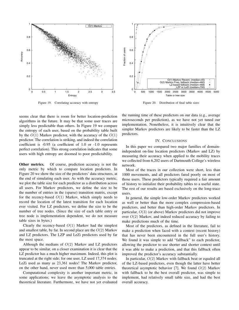
Figure 19. Correlating accuracy with entropy

seems clear that there is room for better location-predictionalgorithms in the future. It may be that some user traces aresimply less predictable than others. In Figure 19 we comparethe entropy of each user, based on the probability table builtby the O(1) Markov predictor, with the accuracy of the O(1)predictor. The correlation is striking, and indeed the correlationcoefficient is -0.95 (a coefficient of 1.0 or -1.0 representsperfect correlation). This strong correlation indicates that someusers with high entropy are doomed to poor predictability.

Other metrics. Of course, prediction accuracy is not theonly metric by which to compare location predictors. InFigure 20 we show the size of the predictors’ data structures, atthe end of simulating each user. As with the accuracy metric,we plot the table size for each predictor as a distribution acrossall users. For Markov predictors, we define the size to bethe number of entries in the (sparse) transition matrix, exceptfor the recency-based O(1) Markov, which simply needs torecord the location of the latest transition for each locationever visited. For LZ predictors, we define the size to be thenumber of tree nodes. (Since the size of each table entry ortree node is implementation dependent, we do not measuretable sizes in bytes.)

Clearly the recency-based O(1) Markov had the simplestand smallest table, by far. In second place are the O(2) Markovand LZ predictors. The LZP and LeZi predictors used by farthe most space.

Although the medians of O(2) Markov and LZ predictorsappear to be similar, on a closer examination it is clear that theLZ predictor has a much higher maximum. Indeed, this plot istruncated at the right side; for one user, LZ used 17,374 nodes.LeZi used as many as 23,361 nodes! The Markov predictor,on the other hand, never used more than 5,000 table entries.

Computational complexity is another important metric, insome applications; we leave the asymptotic analysis to thetheoretical literature. Furthermore, we have not yet evaluated

0

0.2

0.4

0.6

0.8

1

0 500 1000 1500 2000 2500 3000 3500 4000 4500 5000

Fra

ctio

n of

use

rs

Table or tree size

O(1) Markov Recent. (median=45)O(2) Markov Freq. fallback (median=460)

LZ-based fallback (median=468)LZP or LeZi (median=700)

Figure 20. Distribution of final table sizes

the running time of these predictors on our data (e.g., averagemicroseconds per prediction), as we have not yet tuned ourimplementation. Nonetheless, it is intuitively clear that thesimpler Markov predictors are likely to be faster than the LZpredictors.

IV. CONCLUSIONS

In this paper we compared two major families of domain-independent on-line location predictors (Markov and LZ) bymeasuring their accuracy when applied to the mobility traceswe collected from 6,202 users of Dartmouth College’s wirelessnetwork.

Most of the traces in our collection were short, less than1000 movements, and all predictors fared poorly on most ofthose users. These predictors typically required a fair amountof history to initialize their probability tables to a useful state.The rest of our results are based exclusively on the long-traceusers.

In general, the simple low-order Markov predictors workedas well or better than the more complex compression-basedpredictors, and better than high-order Markov predictors. Inparticular, O(3) (or above) Markov predictors did not improveover O(2) Markov, and indeed reduced accuracy by failing tomake predictions much of the time.

Most of the predictors, as defined in the literature, fail tomake a prediction when faced with a context (recent history)that has never been encountered in the full user’s history.We found it was simple to add “fallback” to each predictor,allowing the predictor to use shorter and shorter context untilit was able to make a prediction, and that this fallback oftenimproved the predictor’s accuracy substantially.

In particular, O(2) Markov with fallback beat or equaled allof the LZ-based predictors, even though the latter have bettertheoretical asymptotic behavior [7]. We found O(2) Markovwith fallback to be the best overall predictor, was simple toimplement, had relatively small table size, and had the bestoverall accuracy.

Copyright IEEE INFOCOM 2004 10

We experimented with a simple alternative to the frequency-based approach to Markov predictors, using recency (proba-bility 1 for most recent, 0 for all other) to define the transitionmatrix. Although this recency approach was best amongO(1) Markov predictors, it was worst among O(2) Markovpredictors, and we are still investigating the underlying reason.

We found most of the literature defining these predictorsto be remarkably insufficient at defining the predictors forimplementation. In particular, none defined how the predictorshould behave in the case of a tie, that is, when there wasmore than one location with the same most-likely probability.We investigated a variety of tie-breaking schemes within theMarkov predictors, but found that the accuracy distributionwas not sensitive to the choice.

Since some of our user traces extend over weeks or months,it is possible that the user’s mobility patterns do change overtime. All of our predictors assume the probability distributionsare stable. We briefly experimented with extensions to theMarkov predictors that “age” the probability tables so thatmore recent movements have more weight in computingthe probability, but the accuracy distributions did not seemsignificantly affected. We need to study this issue further.

We examined the original LZ predictor as well as twoextensions, prefix and PPM. LZ with both extensions is knownas LeZi. We found that both extensions did improve the LZpredictor’s accuracy, but that the simple addition of fallbackto LZ did just as well, was much simpler, and had a muchsmaller data structure. To be fair, PPM tries to do more thanwe require, to predict the future path (not just the next move).

We stress that all of our conclusions are based on our ob-servations of the predictors operating on over 2000 users, andin particular whether a given predictor’s accuracy distributionseems better than another predictor’s accuracy distribution.For an individual user the outcome may be quite differentthan in our conclusion. We plan to study the characteristicsof individual users that lead some to be best served by onepredictor and some to be best served by another predictor.

There was a large gap between the predictor’s accuracydistribution and the “optimal” accuracy bound, indicatingthat there is substantial room for improvement in locationpredictors. On the other hand, our optimal bound may beoverly optimistic for realistic predictors, since it assumes thata predictor will predict accurately whenever the device is at alocation it has visited before. We suspect that domain-specificpredictors will be necessary to come anywhere close to thisbound.

Overall, the best predictors had an accuracy of about 65–72% for the median user. On the other hand, the accuracyvaried widely around that median. Some applications maywork well with such performance, but many applications willneed more accurate predictors; we encourage further researchinto better predictors.

We continue to collect syslog data, extending and expandingour collection of user traces. We plan to evaluate domain-specific predictors, develop new predictors, and develop newaccuracy metrics that better suit the way applications use

location predictors. We also plan to predict the location alongwith the time in the future.

ACKNOWLEDGEMENTS

The Dartmouth authors thank DoCoMo USA Labs, for theirfunding of this research, and Cisco Systems, for their fundingof the data-collection effort. We thank the staff of ComputerScience and Computing Services at Dartmouth College fortheir assistance in collecting the data.

REFERENCES

[1] David A. Levine, Ian F. Akyildiz, and Mahmoud Naghshineh, “Theshadow cluster concept for resource allocation and call admission inATM-based wireless networks,” in Mobile Computing and Networking,1995, pp. 142–150.

[2] William Su and Mario Gerla, “Bandwidth allocation strategies forwireless ATM networks using predictive reservation,” in Proceedings ofGlobal Telecommunications Conference (IEEE Globecom), November1998, vol. 4, pp. 2245–2250.

[3] George Liu and Gerald Maguire Jr., “A class of mobile motion predic-tion algorithms for wireless mobile computing and communications,”ACM/Baltzer Mobile Networks and Applications (MONET), vol. 1, no.2, pp. 113–121, 1996.

[4] Sajal K. Das and Sanjoy K. Sen, “Adaptive location prediction strategiesbased on a hierarchical network model in a cellular mobile environment,”The Computer Journal, vol. 42, no. 6, pp. 473–486, 1999.

[5] Amiya Bhattacharya and Sajal K. Das, “LeZi-Update: An information-theoretic approach to track mobile users in PCS networks,” ACM/KluwerWireless Networks, vol. 8, no. 2-3, pp. 121–135, March–May 2002.

[6] Fei Yu and Victor C. M. Leung, “Mobility-based predictive call admis-sion control and bandwidth reservation in wireless cellular networks,”Computer Networks, vol. 38, no. 5, pp. 577–589, 2002.

[7] Christine Cheng, Ravi Jain, and Eric van den Berg, “Location predictionalgorithms for mobile wireless systems,” in Handbook of WirelessInternet, M. Illyas and B. Furht, Eds. CRC Press, 2003.

[8] Sajal K. Das, Diane J. Cook, Amiya Bhattacharya, Edwin Heierman,and Tze-Yun Lin, “The role of prediction algorithms in the MavHomesmart home architecture,” IEEE Wireless Communications, vol. 9, no.6, pp. 77–84, 2002.

[9] Jeffrey Scott Vitter and P. Krishnan, “Optimal prefetching via datacompression,” Journal of the ACM, vol. 43, no. 5, pp. 771–793, 1996.

[10] Jacob Ziv and Abraham Lempel, “Compression of individual sequencesvia variable-rate coding,” IEEE Transactions on Information Theory,vol. 24, no. 5, pp. 530–536, Sept. 1978.

[11] P. Krishnan and Jeffrey Scott Vitter, “Optimal prediction for prefetchingin the worst case,” SIAM Journal on Computing, vol. 27, no. 6, pp.1617–1636, 1998.

[12] Meir Feder, Neri Merhav, and Michael Gutman, “Universal predictionof individual sequences,” IEEE Transactions on Information Theory,vol. 38, no. 4, pp. 1258–1270, July 1992.

[13] Timothy C. Bell, John G. Cleary, and Ian H. Witten, Text Compression,Prentice Hall, 1990.

[14] David Kotz and Kobby Essien, “Analysis of a campus-wide wirelessnetwork,” in Proceedings of the Eighth Annual International Conferenceon Mobile Computing and Networking, September 2002, pp. 107–118,Revised and corrected as Dartmouth CS Technical Report TR2002-432.

[15] David Kotz and Kobby Essien, “Analysis of a campus-wide wirelessnetwork,” ACM Mobile Networks and Applications (MONET), 2003,Accepted for publication.

Copyright IEEE INFOCOM 2004 11