MME 3514 MATERIALS

THERMODYNAMICS

Partial and Excess Properties

Recall that partial properties of components in solution are their share of the

total solution property

These important equations relating total extensive properties including V, H, G, S,

U to partial properties apply to binary solutions in the following form:

𝑀 = 𝑥𝑖𝑀𝑖𝑖

𝑑𝑀 = 𝑀𝑖𝑑𝑥𝑖𝑖

𝑥𝑖𝑑𝑀𝑖𝑖

= 0

𝑀 = 𝑥𝐴𝑀𝐴 + 𝑥𝐵𝑀𝐵

𝑥𝐴𝑑𝑀𝐴 + 𝑥𝐵𝑑𝑀𝐵 = 0

𝑑𝑀 = 𝑀𝐴𝑑𝑥𝐴 +𝑀𝐵𝑑𝑥𝐵

Partial properties of components in a binary solution can be obtained if the total

solution property is represented as a function of composition

𝑉𝐴 = 𝑉 + 𝑥𝐵𝑑𝑉

𝑑𝑥𝐴

𝑉𝐵 = 𝑉 − 𝑥𝐴𝑑𝑉

𝑑𝑥𝐴

Example – The enthalpy of a binary liquid system of species 1 and 2 at fixed T

and P is represented by the equation

Determine expressions for 𝐻1 and 𝐻2

𝐻1 = 𝐻 + 𝑥2𝑑𝐻

𝑑𝑥1

𝐻2 = 𝐻 − 𝑥1𝑑𝐻

𝑑𝑥1

𝐻 = 400𝑥1 + 600𝑥2 + 𝑥1𝑥2(40𝑥1 + 20𝑥2) J/mole

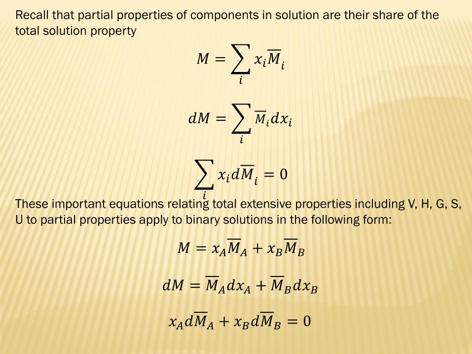
Further derivation of the fundamental partial property equations enable

determination of the partial property of one component if the variation of the

other’s as a function of composition is known

substituting by 𝑥𝐴 = 1 − 𝑥𝐵 yields

𝑀𝐵 is constant at 𝑥𝐵 = 1 and equals 𝑀𝐵𝑜while

1−𝑥𝐵

𝑥𝐵 equals 0

So the equation can be integrated between limits 𝑀𝐵 and 𝑀𝐵𝑜

𝑀𝐵 is obtained from the integration by adding 𝑀𝐵𝑜 directly if 𝑀𝐴 = 𝑓 𝑥𝐵 is

known

Graphical determination of 𝑀𝐵 −𝑀𝐵𝑜 is possible by plotting a

1−𝑥𝐵

𝑥𝐵- 𝑀𝐴 graph

𝑥𝐴𝑑𝑀𝐴 + 𝑥𝐵𝑑𝑀𝐵 = 0

𝑑𝑀𝐵 = −1 − 𝑥𝐵𝑥𝐵

𝑑𝑀𝐴

𝑑𝑀𝐵

𝑀𝐵

𝑀𝐵𝑜

= 𝑀𝐵 −𝑀𝐵𝑜 =

1 − 𝑥𝐵𝑥𝐵

𝑑𝑀𝐴

(𝑀𝐴)𝑋𝐵=𝑎

(𝑀𝐴)𝑋𝐵=1

The area under the curve between the limits (𝑉𝐴)𝑋𝐵=1 and (𝑉

𝐴)𝑋𝐵=𝑎 gives

𝑉𝐵 − 𝑉𝐵𝑜

𝑉𝐵 − 𝑉𝐵𝑜 =

1 − 𝑥𝐵𝑥𝐵

𝑑𝑉𝐴

(𝑉𝐴)𝑋𝐵=𝑎

(𝑉𝐴)𝑋𝐵=1

𝑉𝐵 − 𝑉𝐵𝑜 = 𝑦𝑑𝑈

𝑈2

𝑈1

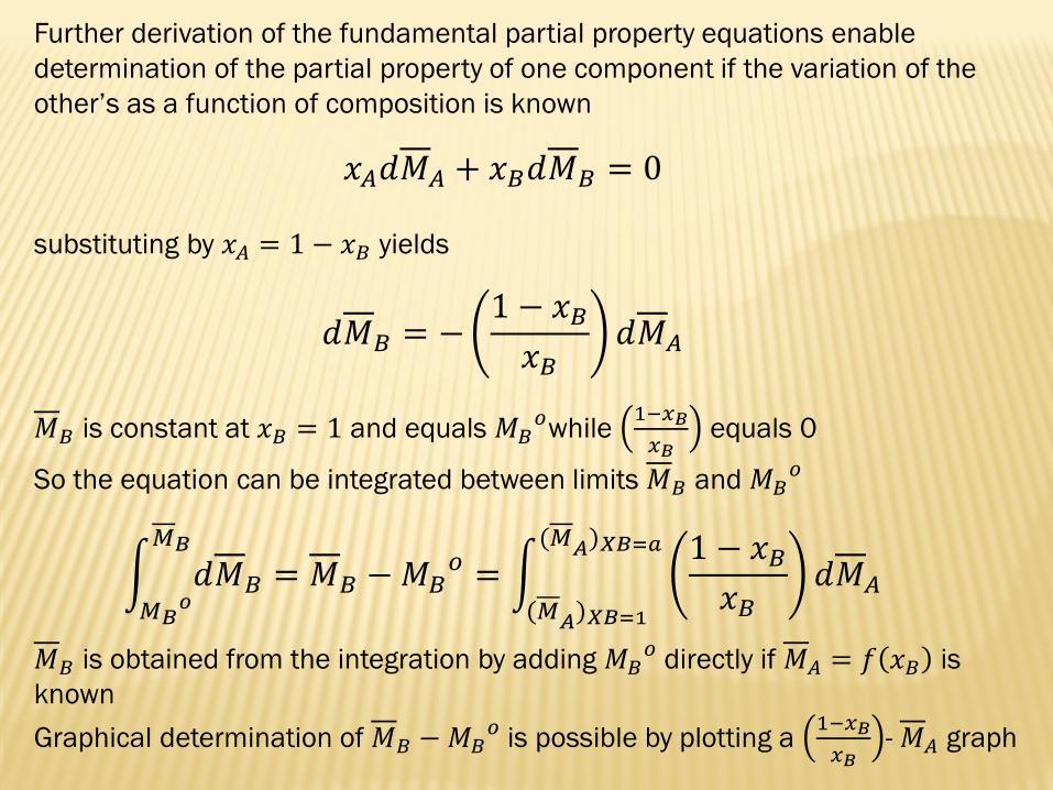
Activity of a component in a binary solution can be obtained from that of other by

a similar approach:

Replacing by 𝑑𝐺𝐴 = 𝑅𝑇𝑑 ln 𝑎𝐴 yields

Further substituting by 𝑥𝐴 = 1 − 𝑥𝐵 and arranging,

Integrating the above equation between 𝑎𝐴 = 1 at 𝑥𝐵 = 0 and 𝑎𝐴 is not possible

as ln 𝑎𝐵 = −∞ at 𝑥𝐵 = 0

𝑥𝐴𝑑𝐺𝐴 + 𝑥𝐵𝑑𝐺𝐵 = 0

𝑥𝐴𝑑 ln 𝑎𝐴 + 𝑥𝐵𝑑 ln 𝑎𝐵 = 0

𝑑 ln 𝑎𝐴 = −𝑥𝐵1 − 𝑥𝐵

𝑑 ln 𝑎𝐵

Instead of using activity of components which is a strong function of composition,

activity coefficient may be used by replacing with 𝑎𝑖 = 𝛾𝑖𝑥𝑖

since 𝑥𝑖𝑑 ln 𝑥𝑖 = 𝑑𝑥𝑖, 𝑥𝐴 + 𝑥𝐵 = 1 and 𝑑𝑥𝐴 + 𝑑𝑥𝐵 = 0,

Integrating the above equation between 𝛾𝐴 = 1 at 𝑥𝐵 = 0 and 𝑎𝐴 gives ln 𝛾𝐴

𝑥𝐴𝑑 ln 𝛾𝐴 + 𝑥𝐵𝑑 ln 𝛾𝐵 +𝑥𝐴𝑑 ln 𝑥𝐴 + 𝑥𝐵𝑑 ln 𝑥𝐵 = 0

𝑑 ln 𝛾𝐴 = −𝑥𝐵1 − 𝑥𝐵

𝑑 ln 𝛾𝐵

𝑥𝐴𝑑 ln 𝑎𝐴 + 𝑥𝐵𝑑 ln 𝑎𝐵 = 0

𝑥𝐴𝑑 ln 𝛾𝐴 + 𝑥𝐵𝑑 ln 𝛾𝐵 = 0

Activity coefficient is an auxillary function that relates compositions of the

components in a real solution to their activities

Relationships that are derived for ideal solutions based on the neutrality of the

components of the model solution can be adjusted to real solutions by the activity

coefficient

Activity coefficient indicates the deviation of components of a real solution from

ideal behavior due to the interaction of molecules

A and B molecules attract eachother when their activities are less than their

compositions and repel eachother when activities are greater

If 𝛾𝑖 > 1, solution positively deviates from Raoult’s law due to repulsion between

two kinds of molecules. Extensive properties of the solution such as volume,

enthalpy, Gibbs free energy increase in this case as well as the partial volume,

enthalpy and Gibbs free energies of the components

If 𝛾𝑖 < 1, solution negatively deviates from Raoult’s law due to attraction between

two kinds of molecules. Extensive properties of both the system and components

decrease in this case

𝑎𝑖 = 𝛾𝑖𝑥𝑖

Positive deviation from ideality Negative deviation from ideality

𝛾𝑖 > 1 𝛾𝑖 < 1

Ideal solution is a model for relating thermodynamic extensive properties to

experimental PVT data

Treatment of all liquid solutions in the same way as ideal solutions enables

complete determination of their thermodynamic properties and equations of state

Excess properties are derived for measuring the deviations of liquid solutions

from ideal solutions for this reason

If M represents the molar value of an extensive thermodynamic property, then an

excess property ME is defined as the difference between the actual property value

of a solution and the value it would have as an ideal solution

𝐺𝑖𝑑 = 𝑥𝑖𝐺𝑖 + 𝑅𝑇 𝑥𝑖ln 𝑥𝑖

𝑆𝑖𝑑 = 𝑥𝑖𝑆𝑖 − 𝑅 𝑥𝑖ln 𝑥𝑖

𝐻𝑖𝑑 = 𝑥𝑖𝐻𝑖

𝜇𝐴𝑖𝑑 = 𝐺𝐴 + 𝑅𝑇 ln 𝑥𝐴

𝑆𝐴𝑖𝑑 = 𝑆𝐴 + 𝑅 ln 𝑥𝐴

𝐻𝐴𝑖𝑑 = 𝐻𝐴

𝑀𝐸 = 𝑀 −𝑀𝑖𝑑

Representation of excess Gibbs free energy which is of most interest is as follows:

The same form of equation follows for partial properties of a solution

The difference between the partial molar Gibbs free energy of a component and

its free energy at pure state is

Similarly for ideal solution:

Taking the difference between the two equations gives the excess partial molar

Gibbs free energy

𝑎𝑖𝑥𝑖= 𝛾𝑖

𝐺𝐸 = 𝐺 − 𝐺𝑖𝑑

𝐺𝑖𝐸= 𝐺𝑖 − 𝐺𝑖

𝑖𝑑

𝐺𝑖 − 𝐺𝑖 = 𝑅𝑇 ln𝑎𝑖𝑎𝑖𝑜=𝑅𝑇 ln 𝑎𝑖

𝐺𝑖𝑖𝑑− 𝐺𝑖 = 𝑅𝑇 ln 𝑥𝑖

𝐺𝑖𝐸= 𝐺𝑖 − 𝐺𝑖

𝑖𝑑= 𝑅𝑇 ln

𝑎𝑖𝑥𝑖

For an ideal solution 𝐺𝑖𝐸= 0, so 𝛾𝑖 = 1

Since 𝐺𝑖𝐸

is a partial property of the total excess Gibbs free energy of the solution,

ln 𝛾𝑖 is also a partial property with respect to 𝐺𝐸/𝑅𝑇

at constant T and P

𝐺𝑖𝐸

𝑅𝑇= 𝑅𝑇 ln 𝛾𝑖

ln 𝛾𝑖 =𝜕 𝑛𝐺𝐸 𝑅𝑇

𝜕𝑛𝑖 𝑃,𝑇,𝑛𝑗

𝐺𝐸

𝑅𝑇= 𝑥𝑖 ln 𝛾𝑖

𝑥𝑖 𝑑 ln 𝛾𝑖 = 0

The usefulness of the equations and the excess property concept in general is the

ability to calculate the extensive properties V, H, S, G, U of any liquid solution by

relating them to ideal solution

Excess properties can be as easily calculated as ideal solution properties

provided that activity coefficients are known in addition to concentration

Excess properties are functions of temperature and solution composition

𝛾𝑖 values are experimentally accessible through vapor/liquid equilibrium data and

mixing experiments through which 𝐺𝐸and 𝐻𝐸are obtained respectively

Excess entropy 𝑆𝐸 is not measured directly but found from the equation:

𝑆𝐸 =𝐻𝐸 − 𝐺𝐸

𝑇

Example – What is the excess volume of 2000 cm3 of antifreeze consisting of 30

mol % methanol in water at 25 °C? Molar volumes of pure species and partial

molar volumes at 25 °C are given as

VM= 40.727 cm3/mol, VMP= 38.632 cm3/mol

VW= 18.068 cm3/mol, VWP= 17.765 cm3/mol

The fundamental excess property relation and its derivations

Gibbs free energy is a generating property for all other related properties

Since 𝐺 = 𝐻 − 𝑇𝑆,

𝑑 𝑛𝐺 =𝜕 𝑛𝐺

𝜕𝑃𝑇,𝑛

𝑑𝑃 +𝜕 𝑛𝐺

𝜕𝑇𝑃,𝑛

𝑑𝑇 + 𝜕 𝑛𝐺

𝜕𝑛𝑖 𝑃,𝑇,𝑛𝑗

𝑑𝑛𝑖𝑖

𝑑 𝑛𝐺 = (𝑛𝑉)𝑑𝑃 + (𝑛𝑆)𝑑𝑇 + 𝜇𝑖𝑑𝑛𝑖𝑖

𝑑𝑛𝐺

𝑅𝑇=1

𝑅𝑇𝑑 𝑛𝐺 −

𝑛𝐺

𝑅𝑇2𝑑𝑇

𝑑𝑛𝐺

𝑅𝑇=(𝑛𝑉)𝑑𝑃 + (𝑛𝑆)𝑑𝑇 + 𝜇𝑖𝑑𝑛𝑖𝑖

𝑅𝑇−𝑛𝐻 − 𝑇𝑛𝑆

𝑅𝑇2𝑑𝑇

𝑑𝑛𝐺

𝑅𝑇=𝑛𝑉

𝑅𝑇𝑑𝑃 −𝑛𝐻

𝑅𝑇2𝑑𝑇 +

𝐺𝑖𝑅𝑇𝑑𝑛𝑖

𝑑𝑛𝐺𝐸

𝑅𝑇=𝑛𝑉𝐸

𝑅𝑇𝑑𝑃 −𝑛𝐻𝐸

𝑅𝑇2𝑑𝑇 + ln𝛾𝑖 𝑑𝑛𝑖

ln 𝛾𝑖 =𝜕 𝑛𝐺𝐸 𝑅𝑇

𝜕𝑛𝑖 𝑃,𝑇,𝑛𝑗

𝜕 ln 𝛾𝑖𝜕𝑃

𝑇,𝑥

=𝑉𝑖𝐸

𝑅𝑇 𝜕 ln 𝛾𝑖𝜕𝑇

𝑃,𝑥

= −𝐻𝑖𝐸

𝑅𝑇2

The mole fractions of a component in a system comprising of a vapor mixture and

a liquid solution are given as yi and xi

Modified Raoult’s law takes into account the deviations from ideality in the liquid

phase and is applicable at low to moderate pressures:

Example – Consider the ethyl ketone – toluene system at 50 C

𝛾𝑖𝑥𝑖𝑃𝑖𝑠𝑎𝑡 = 𝑦𝑖𝑃

𝛾𝑖 =𝑎𝑖𝑥𝑖=𝑃𝑖𝑥𝑖𝑃𝑖𝑜 =𝑦𝑖𝑃

𝑥𝑖𝑃𝑖𝑠𝑎𝑡

𝐺𝐸

𝑅𝑇= 𝑥𝑖 ln 𝛾𝑖

The figures are characteristic of systems with positive deviations from Raoult’s

law,

The points representing ln 𝛾𝑖 tend toward zero as 𝑥𝑖 goes to 1

Thus the activity coefficient of a species in solution becomes unity as the

species becomes pure

At the other limit where 𝑥𝑖 goes to zero and species i becomes infinitely dilute,

ln 𝛾𝑖 is seen to approach some finite limit ln 𝛾𝑖∞

so

𝛾𝑖 ≥ 1 ln 𝛾𝑖 ≥ 0

lim𝑥1→0

𝐺𝐸

𝑅𝑇= 0 ln 𝛾𝑖

∞+ 1 0 = 0

According to the Gibbs-Duhem equation,

a direct relation is seen between the slopes of

curves drawn through the data points for

ln 𝛾1and ln 𝛾2

The slope of the ln 𝛾1 curve is of opposite sign to the slope of the ln 𝛾2 curve

The slope of the ln 𝛾1 curve is zero when 𝑥1 goes to 1

The slope of the ln 𝛾2 curve is zero when 𝑥2 goes to 1

Thus each ln 𝛾𝑖 curve becomes horizontal as 𝑥𝑖 = 1

𝑥𝑖 𝑑 ln 𝛾𝑖 = 0

𝑥1𝑑 ln 𝛾1𝑑𝑥1+ 𝑥2𝑑 ln 𝛾2𝑑𝑥1= 0

𝑑 ln 𝛾1𝑑𝑥1= −𝑥2𝑥1

𝑑 ln 𝛾2𝑑𝑥1= 0

Excess properties have common features:

• All excess properties become zero as either species aprroaches purity

• Both 𝐻𝐸 and 𝑇𝑆𝐸exhibit different composition dependencies although 𝐺𝐸vs x

is nearly parabolic in shape

• The minimum and

maximum of the curves

often occur near the

equimolar

concentration when the

property has a single

sign as 𝐺𝐸 in all six

figures

The signs and relative

magnitudes of 𝐻𝐸, 𝑆𝐸and 𝐺𝐸 are useful for

qualitative engineering

purposes

Excess properties of 135 binary liquid mixtures at fixed temperature of 298 K and

x1=x2=0.5, have been organized by Abbott

Binary organic and aqueous/organic mixtures have been classified based on

hydrogen bonding of pure species:

Nonpolar (NP)

Polar but nonassociating

(NA)

Polar and association (AS)

135 binary mixtures were

investigated and grouped

into 6 binary mixture types

Observed common patterns and norms of excess properties of binary solutions

About 85% of all mixtures

exhibit positive 𝐺𝐸 or

positive 𝐻𝐸(I,II,III, VI); about

70% have positive 𝐺𝐸and

𝐻𝐸 (I, II)

About 60% of all mixtures

fall in I and IV; only 15% in III

and VI. Enthalpy is more

likely to dominate solution

behavior than entropy

NP/NP mixtures concentrate

in I and VI, 𝐻𝐸 and 𝑆𝐸 are

normally positive for such

mixtures. -0.2< 𝐺𝐸<0.2

NA/NP mixtures usually fall

into I, all 𝐺𝐸, 𝐻𝐸 and 𝑆𝐸are

positive with large values

Relationship of excess properties with property changes of mixing

Excess properties can be represented in their basic form as

where 𝑀 − 𝑥𝑖𝑀𝑖 is known as property change of mixing ΔM

Excess properties can be rewritten as

Excess properties and property changes of mixing are readily calculated from

eachother

𝐺𝐸 = 𝐺 − 𝑥𝑖𝐺𝑖 − 𝑅𝑇 𝑥𝑖ln 𝑥𝑖

𝑆𝐸 = 𝑆 − 𝑥𝑖𝑆𝑖 + 𝑅 𝑥𝑖ln 𝑥𝑖

𝐻𝐸 = 𝐻 − 𝑥𝑖𝐻𝑖

𝑉𝐸 = 𝑉 − 𝑥𝑖𝑉𝑖

𝐺𝐸 = ∆𝐺 − 𝑅𝑇 𝑥𝑖ln 𝑥𝑖

𝑆𝐸 = ∆𝑆 + 𝑅𝑇 𝑥𝑖ln 𝑥𝑖

𝐻𝐸 = ∆𝐻

𝑉𝐸 = ∆𝑉

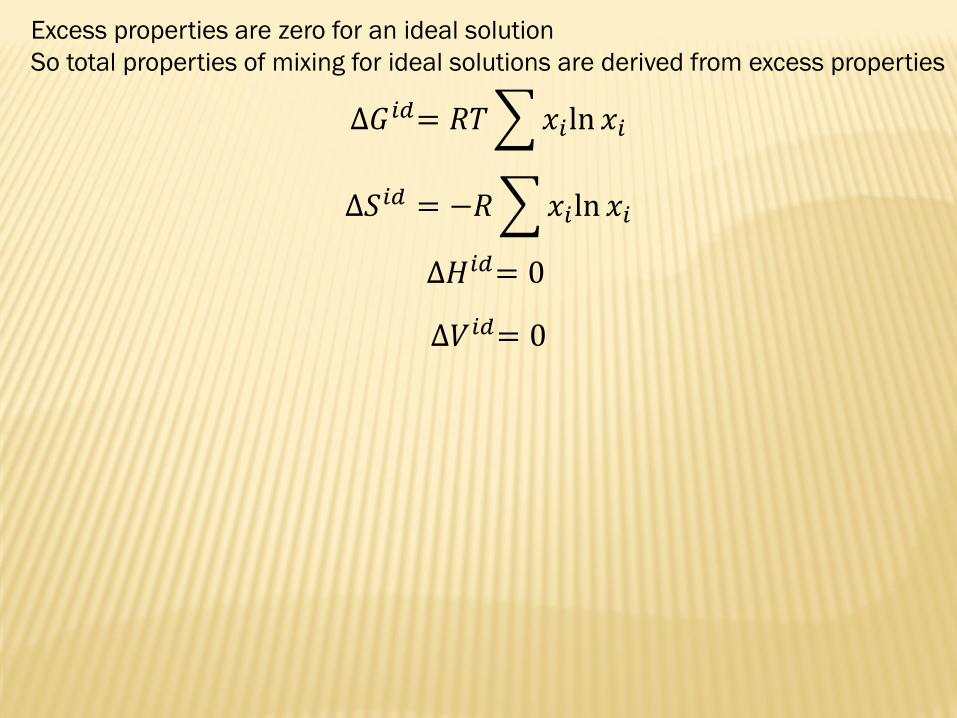
Excess properties are zero for an ideal solution

So total properties of mixing for ideal solutions are derived from excess properties

∆𝐺𝑖𝑑= 𝑅𝑇 𝑥𝑖ln 𝑥𝑖

∆𝑆𝑖𝑑 = −𝑅 𝑥𝑖ln 𝑥𝑖

∆𝐻𝑖𝑑= 0

∆𝑉𝑖𝑑= 0

Property changes of mixing have common features:

• Each ΔM is zero for a pure species

• The Gibbs energy change of mixing ΔG is always negative

• The entropy change

of mixing ΔS>0

Molecular basis for mixture behavior

The relations between excess properties and property changes of mixing enables

discussion of the molecular phenomena which give rise to observed excess

property behavior

Excess enthalpy which equals enthalpy of mixing reflect differences in the

strengths of intermolecular attraction between pairs of unlike species and pairs

of like species.

Interactions between like species are disrupted in a standard mixing process and

interactions between unlike species are promoted

More energy (ΔH) is required in the mixing process to break like attractions if the

unlike attractions are weaker than the average of those between like species

In this case mixing is endothermic, ΔH=HE>0

ΔH=HE<0 if the unlike attractions are stronger and mixing process is exothermic

Observations made from Abbott’s analysis of NP/NP binary mixtures is that

dispersion forces are the only significant attractive intermolecular forces for

NP/NP mixtures. Dispersion forces between unlike species are weaker than the

average of dispersion forces between like species. Hence a positive excess

enthalpy is usually observed for NP/NP mixtures

Example – The excess enthalpy or heat of mixing for a liquid mixture of species 1

and 2 at fixed T and P is represented as

Determine expressions for 𝐻𝐸1 , 𝐻 1 and 𝐻𝐸2 , 𝐻 2 as functions of 𝑥1

𝐻1𝐸= 𝐻𝐸 + 𝑥2

𝑑𝐻𝐸

𝑑𝑥1 𝐻2 − 𝐻2

𝑜 = 1 − 𝑥2𝑥2𝑑𝐻1

(𝐻1)𝑋2=𝑎

(𝐻1)𝑋2=1

0

20

40

60

80

100

120

-25 -20 -15 -10 -5 0

x1 x2 HE1 (1-x2)/x2 HE2

0.6 0.4 -7.04 1.5 7.04

0.59 0.41 -7.32916 1.43902 7.32916

0.58 0.42 -7.62048 1.38095 7.62048

0.57 0.43 -7.91372 1.32558 7.91372

0.56 0.44 -8.20864 1.27272 8.20864

0.55 0.45 -8.505 1.22222 8.505

0.54 0.46 -8.80256 1.17391 8.80256

0.53 0.47 -9.10108 1.12766 9.10108

0.52 0.48 -9.40032 1.08333 9.40032

0.51 0.49 -9.70004 1.04081 9.70004

0.5 0.5 -10 1 10

𝐻 = 400𝑥1 + 600𝑥2 + 𝑥1𝑥2(40𝑥1 + 20𝑥2) J/mole