MLS Band Sounding Measurements: Channel Characterization for Mobile and Fixed Airport Surface Communications

ACAST Workshop16 August 2005

David W. Matolak, Indranil SenSchool of EECS and Avionics Engineering Center

Ohio UniversityAthens, OH 45701

phone: 740.593.1241fax: 740.593.0007

email: matolak@ohiou.edu, is809902@ohio.edu

OHIO UNIVERSITYOHIO UNIVERSITYSchool of Electrical Engineering & Computer ScienceSchool of Electrical Engineering & Computer Science

Rafael ApazaFederal Aviation Administration

Aviation Research OfficeBelleville, MI

phone: (734) 487-7327fax: (734) 487-7428

email: rafael.Apaza@faa.gov

Ohio University2

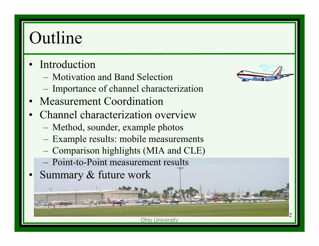
Outline• Introduction

– Motivation and Band Selection– Importance of channel characterization

• Measurement Coordination• Channel characterization overview

– Method, sounder, example photos – Example results: mobile measurements– Comparison highlights (MIA and CLE)– Point-to-Point measurement results

• Summary & future work

Ohio University3

Introduction•• MotivationMotivation

–– Civilian aviation anticipates both a near and longCivilian aviation anticipates both a near and long--term need term need for new communications capabilitiesfor new communications capabilities

•• VHF spectral congestionVHF spectral congestion•• New services desired, both for mobile and New services desired, both for mobile and ““fixedfixed”” servicesservices

•• Band selectionBand selection–– Easiest to quickly deploy system in Easiest to quickly deploy system in ““cleanclean”” spectrumspectrum–– Deployment of new systems to Deployment of new systems to ““protectprotect”” reserved reserved

aeronautical spectrum (aeronautical spectrum (““use it or lose ituse it or lose it””))–– Both these points apply to the MLS extension band, 5.091Both these points apply to the MLS extension band, 5.091--

5.15 GHz, which is not widely used in many regions5.15 GHz, which is not widely used in many regions

Ohio University4

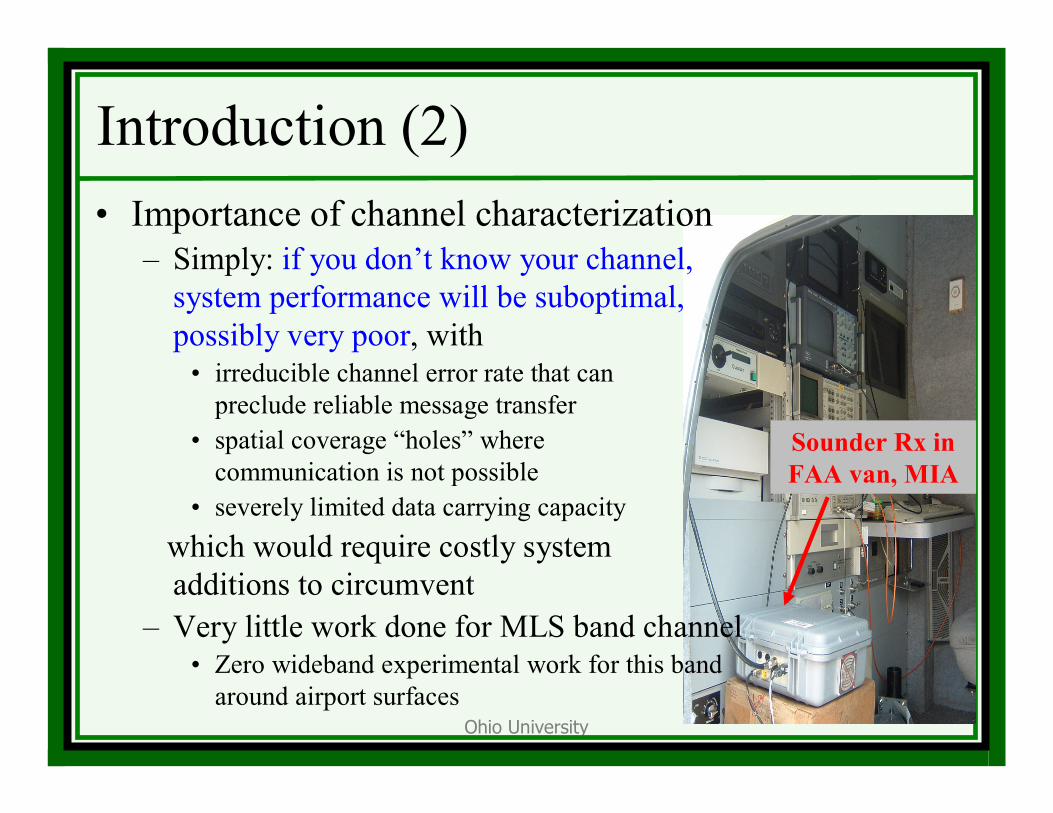
Introduction (2)• Importance of channel characterization

– Simply: if you don’t know your channel, system performance will be suboptimal, possibly very poor, with

• irreducible channel error rate that can preclude reliable message transfer

• spatial coverage “holes” where communication is not possible

• severely limited data carrying capacity which would require costly system additions to circumvent

– Very little work done for MLS band channel• Zero wideband experimental work for this band

around airport surfaces

Sounder Rx in FAA van, MIA

Ohio University5

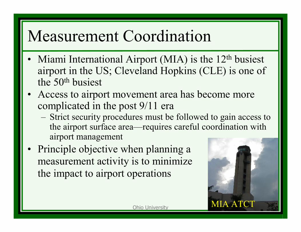
Measurement Coordination• Miami International Airport (MIA) is the 12th busiest

airport in the US; Cleveland Hopkins (CLE) is one of the 50th busiest

• Access to airport movement area has become more complicated in the post 9/11 era – Strict security procedures must be followed to gain access to

the airport surface area—requires careful coordination with airport management

• Principle objective when planning a measurement activity is to minimize the impact to airport operations

MIA ATCT

Ohio University6

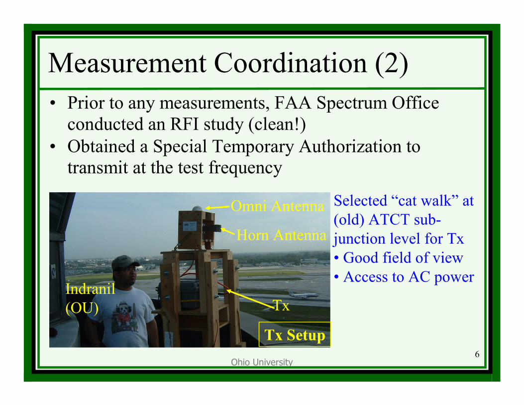
Measurement Coordination (2)• Prior to any measurements, FAA Spectrum Office

conducted an RFI study (clean!)• Obtained a Special Temporary Authorization to

transmit at the test frequency

TxIndranil(OU)

Selected “cat walk” at (old) ATCT sub-junction level for Tx• Good field of view• Access to AC power

Tx Setup

Omni Antenna

Horn Antenna

Ohio University7

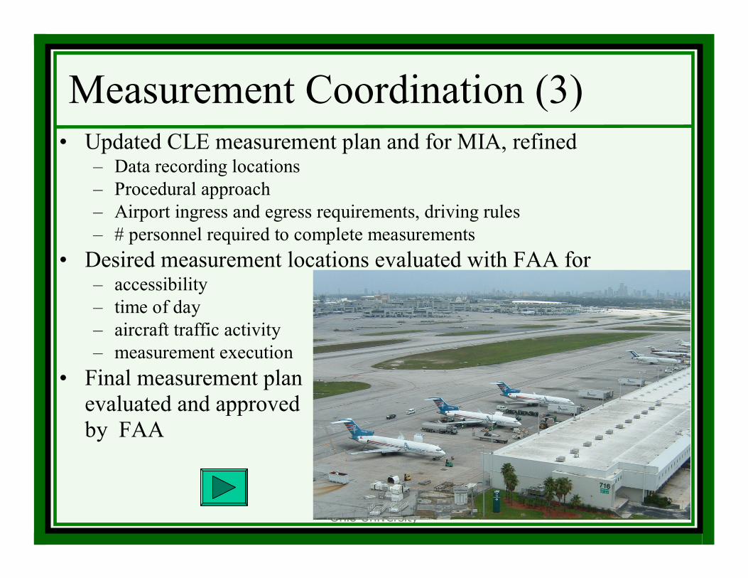
Measurement Coordination (3)• Updated CLE measurement plan and for MIA, refined

– Data recording locations– Procedural approach– Airport ingress and egress requirements, driving rules– # personnel required to complete measurements

• Desired measurement locations evaluated with FAA for– accessibility– time of day– aircraft traffic activity– measurement execution

• Final measurement plan evaluated and approved by FAA

Ohio University8

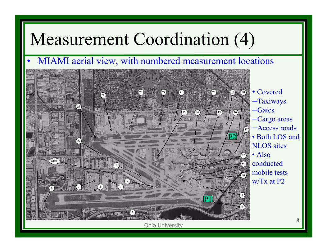
Measurement Coordination (4)• MIAMI aerial view, with numbered measurement locations

• Covered─Taxiways─Gates─Cargo areas─Access roads • Both LOS and NLOS sites• Also conducted mobile tests w/Tx at P2

P2

P1

Ohio University9

∑−

=

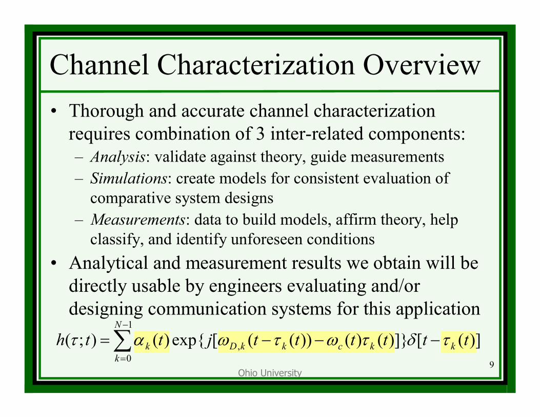
−−−=1

0, )]([)]}()())(([exp{)();(

N

kkkckkDk ttttttjtth τδτωτωατ

Channel Characterization Overview• Thorough and accurate channel characterization

requires combination of 3 inter-related components:– Analysis: validate against theory, guide measurements– Simulations: create models for consistent evaluation of

comparative system designs– Measurements: data to build models, affirm theory, help

classify, and identify unforeseen conditions• Analytical and measurement results we obtain will be

directly usable by engineers evaluating and/or designing communication systems for this application

Ohio University10

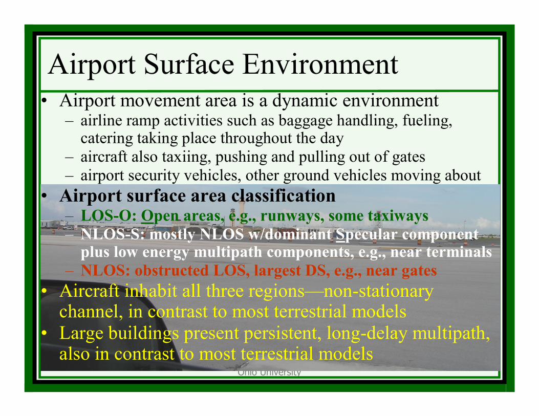
Airport Surface Environment• Airport movement area is a dynamic environment

– airline ramp activities such as baggage handling, fueling, catering taking place throughout the day

– aircraft also taxiing, pushing and pulling out of gates– airport security vehicles, other ground vehicles moving about

• Airport surface area classification– LOS-O: Open areas, e.g., runways, some taxiways– NLOS-S: mostly NLOS w/dominant Specular component

plus low energy multipath components, e.g., near terminals– NLOS: obstructed LOS, largest DS, e.g., near gates

• Aircraft inhabit all three regions—non-stationary channel, in contrast to most terrestrial models

• Large buildings present persistent, long-delay multipath, also in contrast to most terrestrial models

Ohio University11

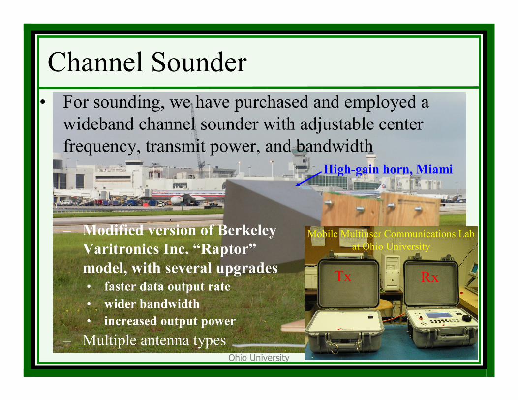
Channel Sounder• For sounding, we have purchased and employed a

wideband channel sounder with adjustable center frequency, transmit power, and bandwidth

– Modified version of Berkeley Varitronics Inc. “Raptor”model, with several upgrades• faster data output rate• wider bandwidth • increased output power

– Multiple antenna types

Tx Rx

Mobile Multiuser Communications Labat Ohio University

High-gain horn, Miami

Ohio University12

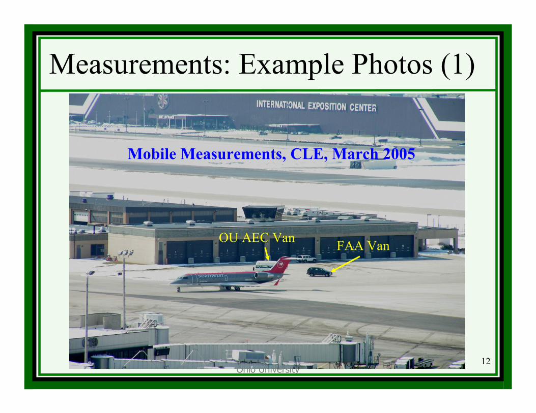
Measurements: Example Photos (1)

OU AEC Van FAA Van

Mobile Measurements, CLE, March 2005

Ohio University13

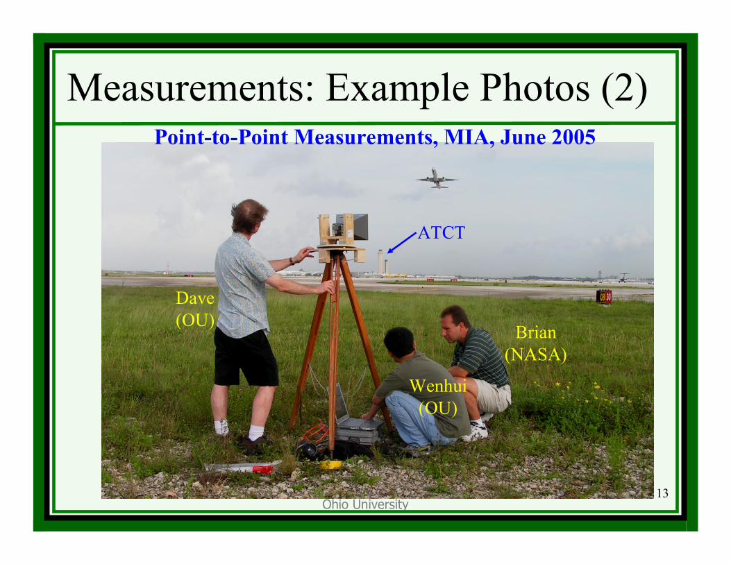
Measurements: Example Photos (2)Point-to-Point Measurements, MIA, June 2005

ATCT

Brian(NASA)

Wenhui(OU)

Dave(OU)

Ohio University14

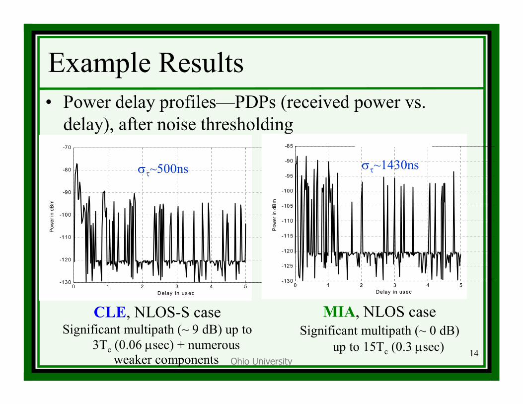
Example Results• Power delay profiles—PDPs (received power vs.

delay), after noise thresholding

CLE, NLOS-S caseSignificant multipath (~ 9 dB) up to

3Tc (0.06 µsec) + numerous weaker components

MIA, NLOS caseSignificant multipath (~ 0 dB)

up to 15Tc (0.3 µsec)

0 1 2 3 4 5-130

-120

-110

-100

-90

-80

-70

Delay in us ec

Pow

er in

dB

m

0 1 2 3 4 5-130

-125

-120

-115

-110

-105

-100

-95

-90

-85Exam ple PDP for a scenario

Delay in usec

Pow

er in

dB

m

στ~500ns στ~1430ns

Ohio University15

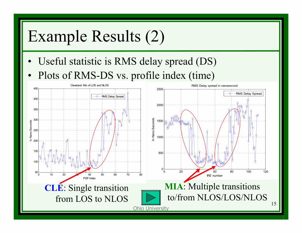
0 10 20 30 40 50 60 70 8050

100

150

200

250

300

350

400

450

PDP Index

In N

ano-

Sec

onds

Cleveland: Mix of LOS and NLOS

RMS Delay Spread

Example Results (2)• Useful statistic is RMS delay spread (DS)• Plots of RMS-DS vs. profile index (time)

CLE: Single transition from LOS to NLOS

MIA: Multiple transitions to/from NLOS/LOS/NLOS

0 20 40 60 80 100 1200

500

1000

1500

2000

2500

IRE number

In N

ano-

Sec

onds

RMS Delay spread in nanosecond

RMS Delay Spread

Ohio University16

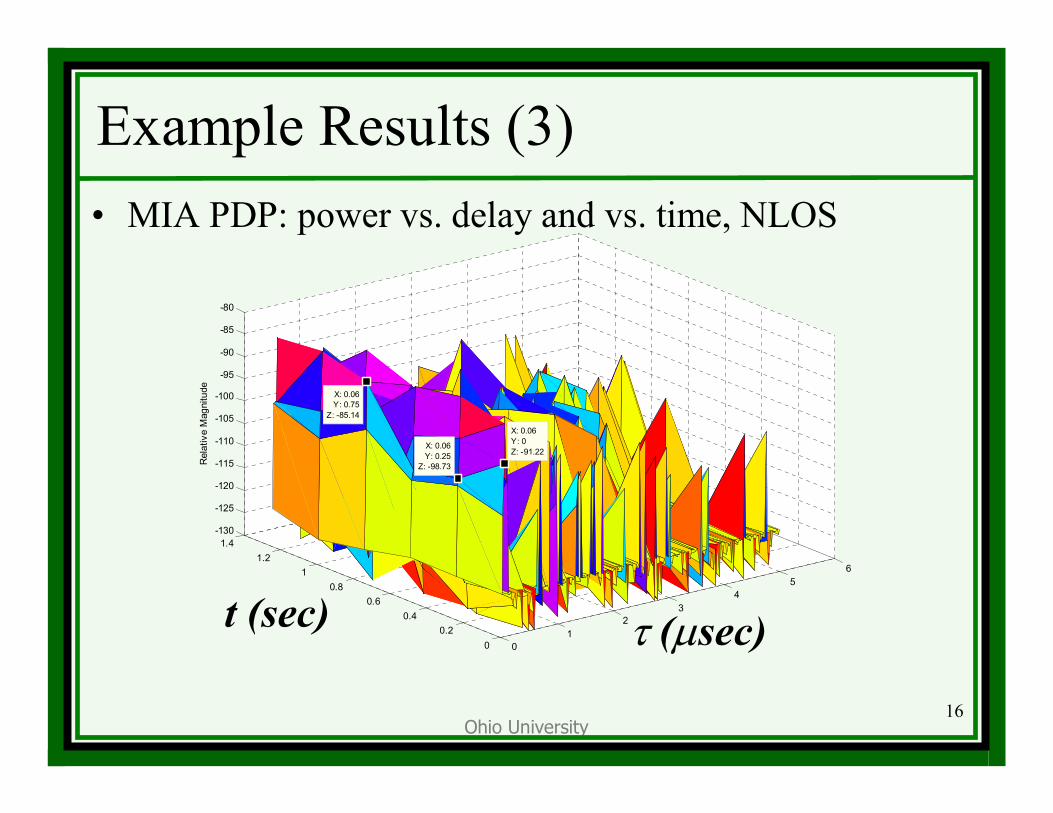
Example Results (3)• MIA PDP: power vs. delay and vs. time, NLOS

τ (µsec)t (sec) 0

12

34

56

00.2

0.40.6

0.81

1.21.4

-130

-125

-120

-115

-110

-105

-100

-95

-90

-85

-80

X: 0.06Y: 0Z: -91.22

X: 0.06Y: 0.25

Z: -98.73

X: 0.06Y: 0.75

Z: -85.14

Rel

ativ

e M

agni

tude

Ohio University17

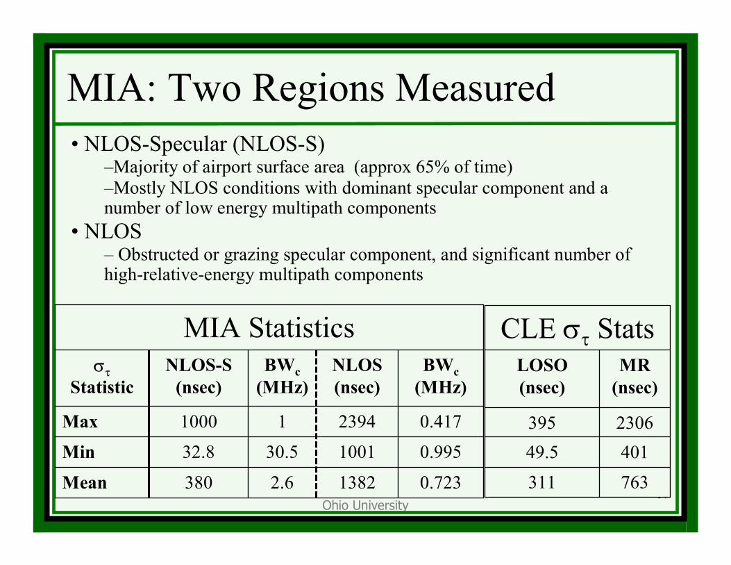
MIA: Two Regions Measured

MIA Statistics

0.72313822.6380Mean

0.995100130.532.8Min

0.417239411000Max

BWc(MHz)

NLOS(nsec)

BWc(MHz)

NLOS-S(nsec)

στStatistic

• NLOS-Specular (NLOS-S) –Majority of airport surface area (approx 65% of time)–Mostly NLOS conditions with dominant specular component and a number of low energy multipath components

• NLOS– Obstructed or grazing specular component, and significant number of high-relative-energy multipath components

CLE στ Stats

76331140149.5

2306395

MR(nsec)

LOSO(nsec)

Ohio University18

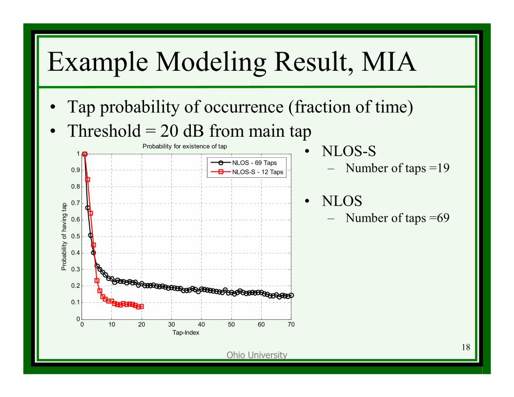
Example Modeling Result, MIA• Tap probability of occurrence (fraction of time)• Threshold = 20 dB from main tap

• NLOS-S– Number of taps =19

• NLOS– Number of taps =69

0 10 20 30 40 50 60 700

0.1

0.2

0.3

0.4

0.5

0.6

0.7

0.8

0.9

1

Tap-Index

Pro

babi

lity

of h

avin

g ta

p

Probability for existence of tap

NLOS - 69 TapsNLOS-S - 12 Taps

Ohio University19

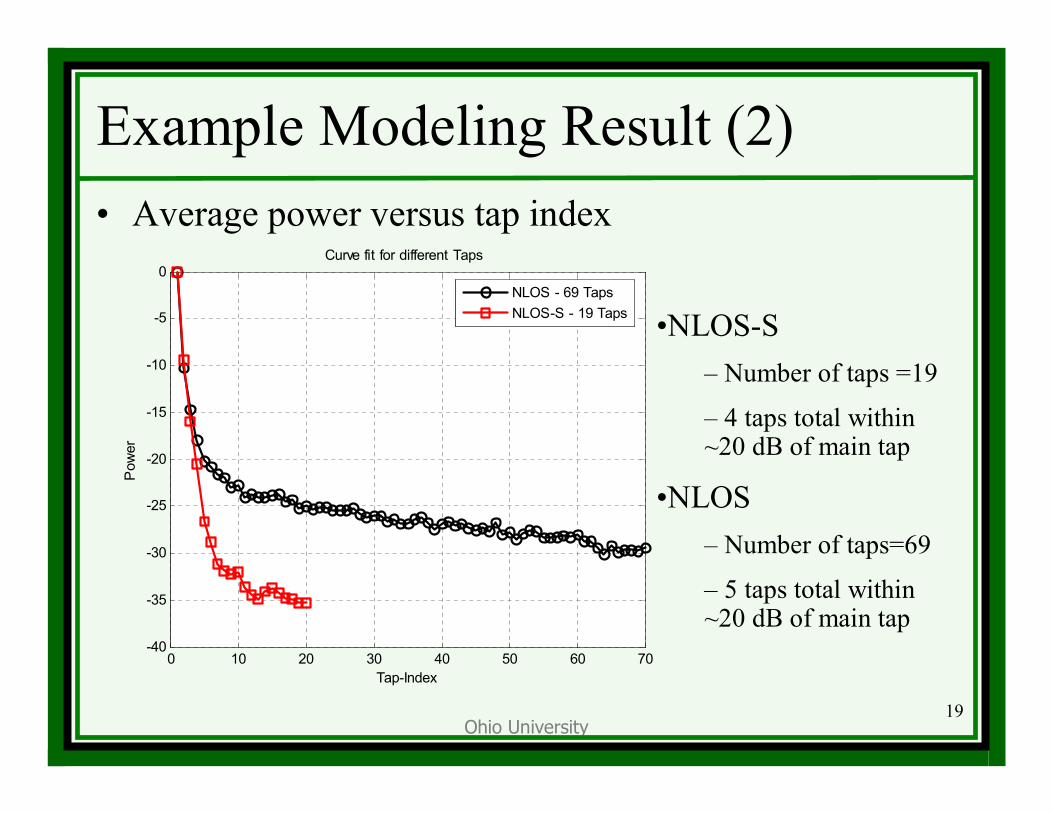
Example Modeling Result (2)• Average power versus tap index

•NLOS-S– Number of taps =19

– 4 taps total within ~20 dB of main tap

•NLOS– Number of taps=69

– 5 taps total within ~20 dB of main tap

0 10 20 30 40 50 60 70-40

-35

-30

-25

-20

-15

-10

-5

0

Tap-Index

Pow

er

Curve fit for different Taps

NLOS - 69 TapsNLOS-S - 19 Taps

Ohio University20

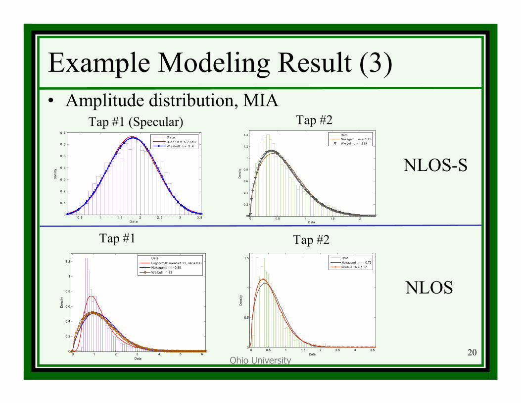
Example Modeling Result (3)• Amplitude distribution, MIA

0.5 1 1 .5 2 2 .5 3 3 .50

0 .1

0 .2

0 .3

0 .4

0 .5

0 .6

0 .7

D a ta

Dens

ity

D a taR ic e : K = 5.7 7 dBW e ib ull: b= 3 .4

0 0.5 1 1.5 20

0.2

0.4

0.6

0.8

1

1.2

1.4

Data

Den

sity

DataNakagami : m = 0.75W eibull: b = 1.629

Tap #1 (Specular) Tap #2

NLOS-S

0 1 2 3 4 5 60

0.2

0.4

0.6

0.8

1

1.2

Data

Den

sity

DataLognormal: mean=1.33, var = 0.6Nakagami : m=0.89Weibull : 1.72

0 0.5 1 1.5 2 2.5 3 3.50

0.5

1

1.5

Data

Den

sity

DataNakagami : m = 0.73Weibull : b = 1.57

Tap #1

NLOS

Tap #2

Ohio University21

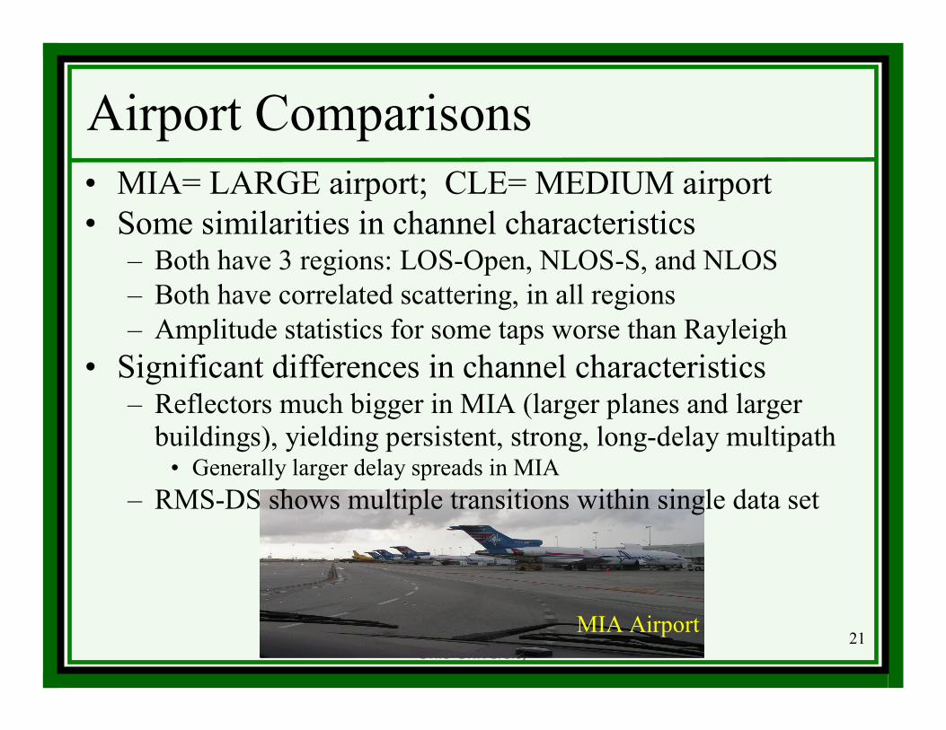
MIA Airport

Airport Comparisons• MIA= LARGE airport; CLE= MEDIUM airport• Some similarities in channel characteristics

– Both have 3 regions: LOS-Open, NLOS-S, and NLOS– Both have correlated scattering, in all regions– Amplitude statistics for some taps worse than Rayleigh

• Significant differences in channel characteristics– Reflectors much bigger in MIA (larger planes and larger

buildings), yielding persistent, strong, long-delay multipath• Generally larger delay spreads in MIA

– RMS-DS shows multiple transitions within single data set

Ohio University22

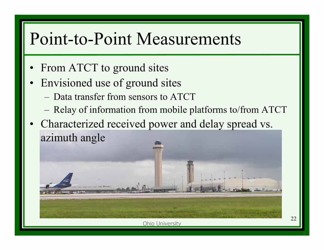
Point-to-Point Measurements• From ATCT to ground sites• Envisioned use of ground sites

– Data transfer from sensors to ATCT– Relay of information from mobile platforms to/from ATCT

• Characterized received power and delay spread vs. azimuth angle

Ohio University23

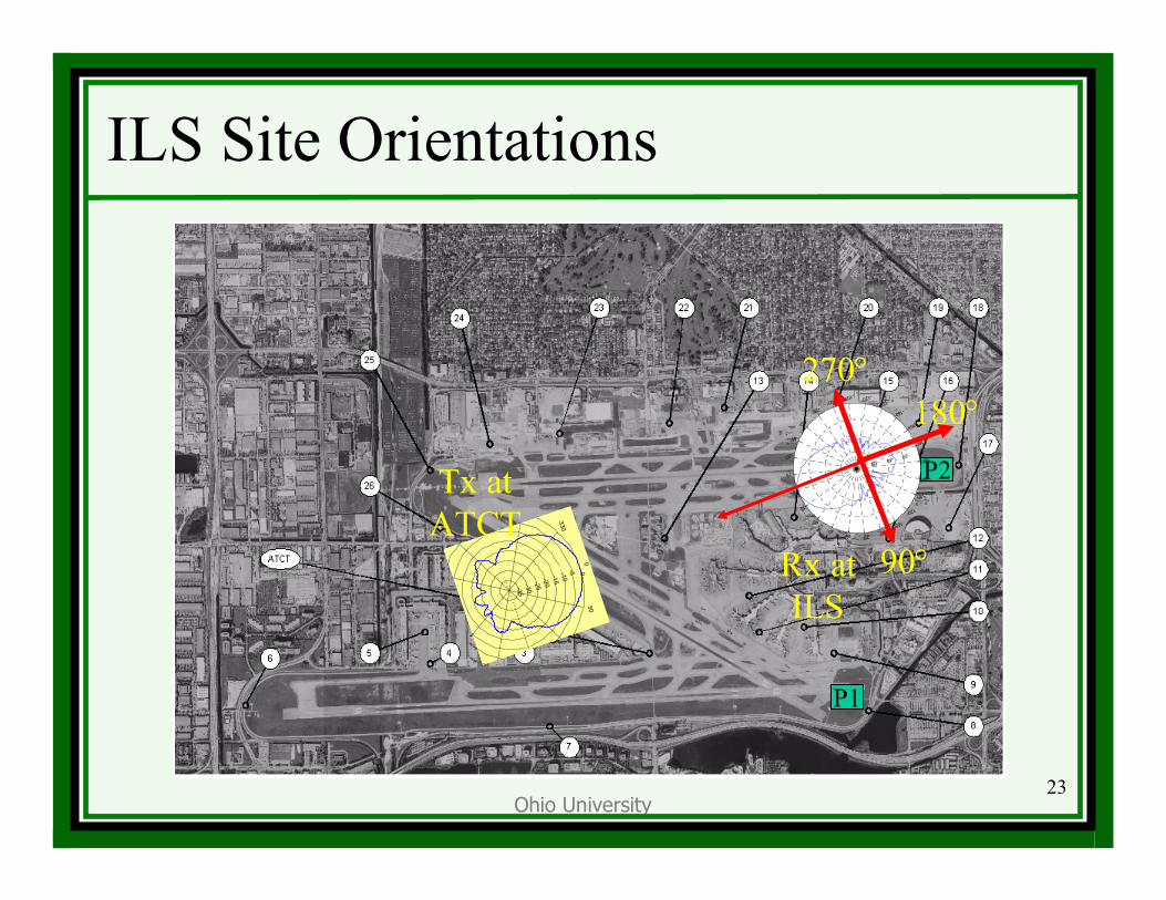
P2

P1

ILS Site Orientations

-35-30

-25-20

-15-10

-5 0

30

330

0 90°

270°180°

Tx atATCT

Rx atILS

0

15°

30°45°

60° 75°90°

105°

120°

135°

150°

165°

±180°

-165°

-150°

-135°

-120°-105°-90°

-75°

-60°

-45°

-30°

-15

-60-40

-200

max=16.7234dB

Ohio University24

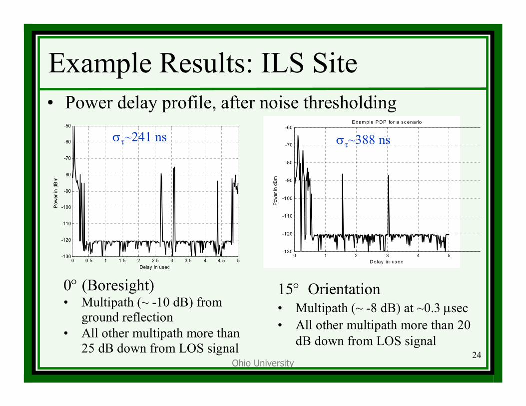
Example Results: ILS Site• Power delay profile, after noise thresholding

0° (Boresight)• Multipath (~ -10 dB) from

ground reflection• All other multipath more than

25 dB down from LOS signal

0 1 2 3 4 5-130

-120

-110

-100

-90

-80

-70

-60E x am ple P DP for a sc enario

Delay in us ec

Pow

er in

dB

m

15° Orientation• Multipath (~ -8 dB) at ~0.3 µsec• All other multipath more than 20

dB down from LOS signal

0 0.5 1 1.5 2 2.5 3 3.5 4 4.5 5-130

-120

-110

-100

-90

-80

-70

-60

-50

Delay in usec

Pow

er in

dB

m

στ~241 ns στ~388 ns

Ohio University25

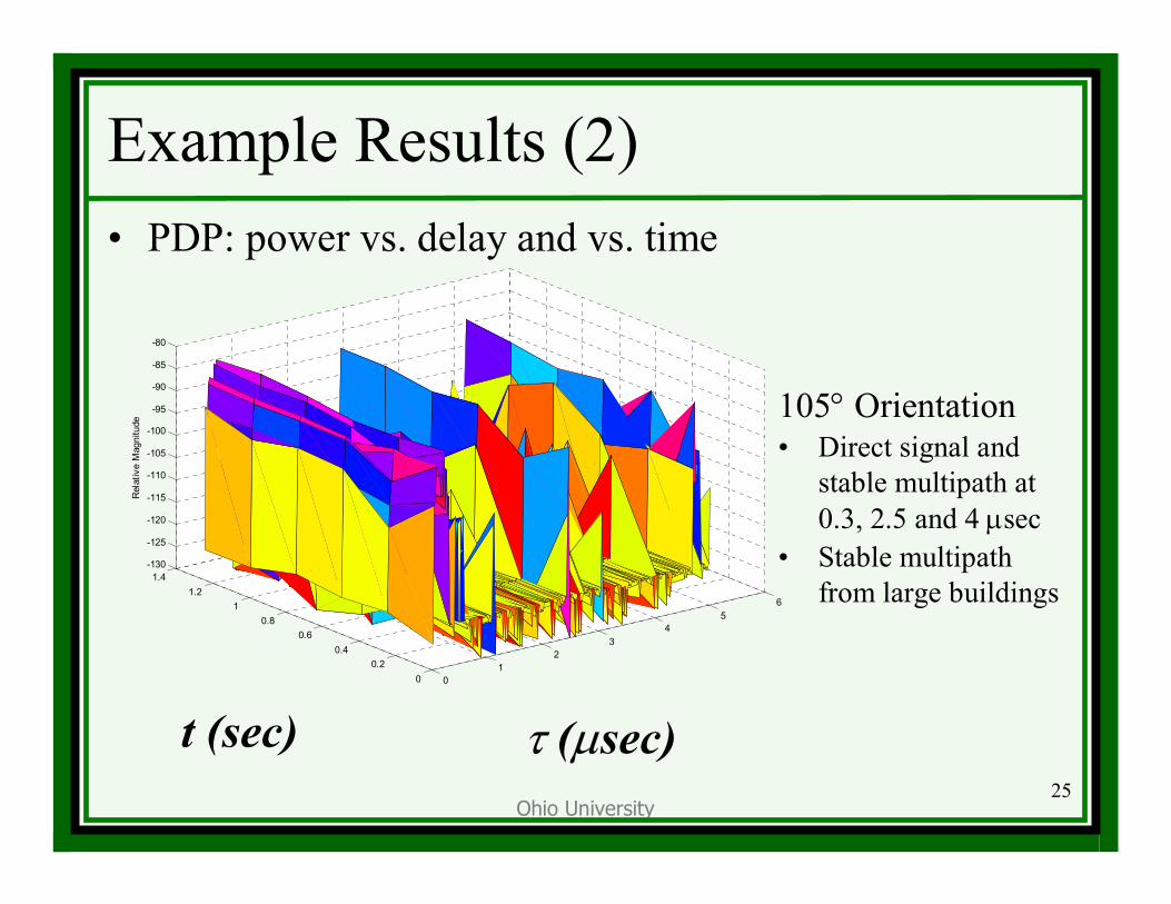
Example Results (2)• PDP: power vs. delay and vs. time

τ (µsec)t (sec) 0

12

34

56

00.2

0.40.6

0.81

1.21.4

-130

-125

-120

-115

-110

-105

-100

-95

-90

-85

-80

Rel

ativ

e M

agni

tude

105° Orientation• Direct signal and

stable multipath at 0.3, 2.5 and 4 µsec

• Stable multipath from large buildings

Ohio University26

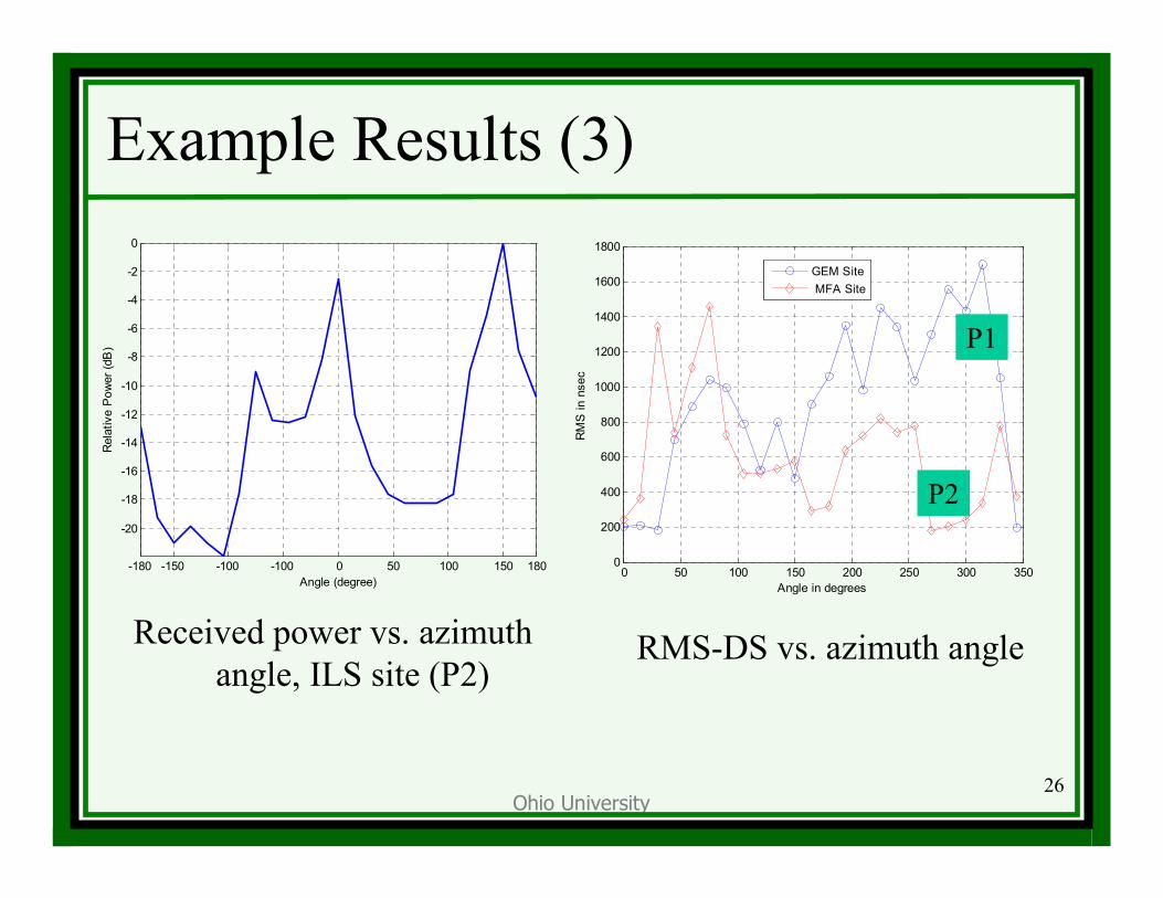
Example Results (3)

Received power vs. azimuth angle, ILS site (P2)

-180 -150 -100 -100 0 50 100 150 180

-20

-18

-16

-14

-12

-10

-8

-6

-4

-2

0

Angle (degree)

Rel

ativ

e P

ower

(dB

)

0 50 100 150 200 250 300 3500

200

400

600

800

1000

1200

1400

1600

1800

Angle in degreesR

MS

in n

sec

GEM Site MFA Site

P1

RMS-DS vs. azimuth angle

P2

Ohio University27

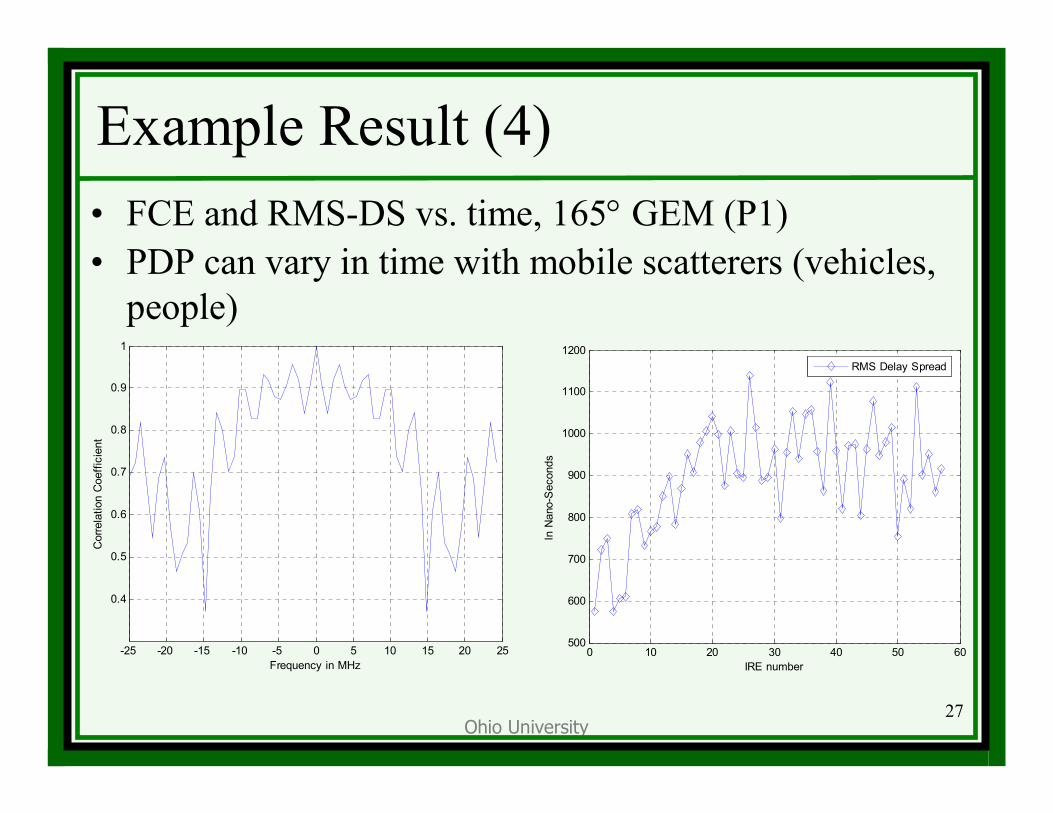
Example Result (4)• FCE and RMS-DS vs. time, 165° GEM (P1)• PDP can vary in time with mobile scatterers (vehicles,

people)

-25 -20 -15 -10 -5 0 5 10 15 20 25

0.4

0.5

0.6

0.7

0.8

0.9

1

Frequency in MHz

Cor

rela

tion

Coe

ffici

ent

0 10 20 30 40 50 60500

600

700

800

900

1000

1100

1200

IRE number

In N

ano-

Sec

onds

RMS Delay Spread

Ohio University28

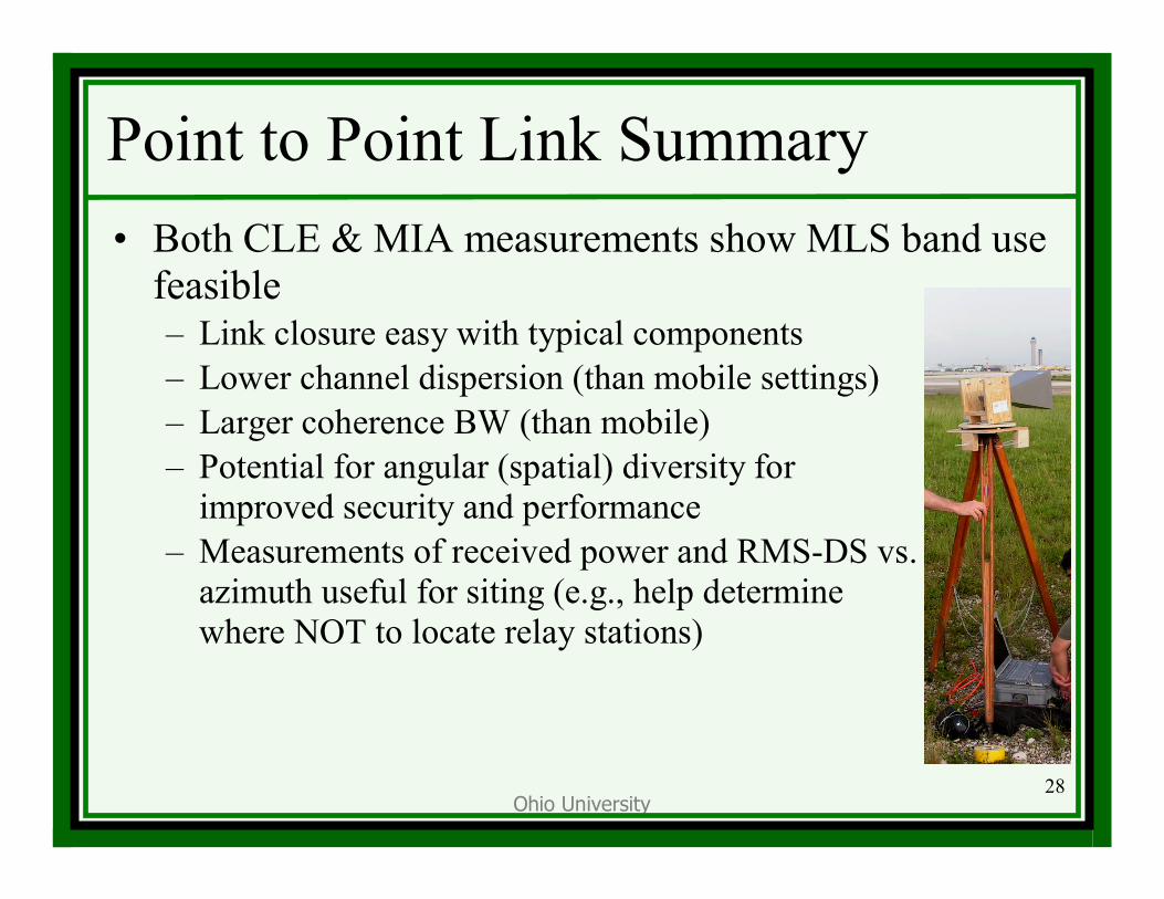
Point to Point Link Summary• Both CLE & MIA measurements show MLS band use

feasible– Link closure easy with typical components– Lower channel dispersion (than mobile settings)– Larger coherence BW (than mobile)– Potential for angular (spatial) diversity for

improved security and performance– Measurements of received power and RMS-DS vs.

azimuth useful for siting (e.g., help determine where NOT to locate relay stations)

Ohio University29

Summary• Provided update on characterization of the 5 GHz MLS

“extension” band channel– Need for effort from the point of view of efficient

communication link design, and band protection• Recent measurement campaigns at CLE and MIA

airports described, including – Coordination w/ local authorities required for successful tests– Short description of equipment, measurement process– Example measured results– Example modeling results– Results for point-to-point links

Ohio University30

Future Work• Gather additional measurement data at one (or two)

more large airports– JFK, 28-31, Aug 2005– Detroit? Fall 2005?

• Completion of data processing • Completion of channel modeling for

– Mobile settings– Point to point settings– “Relay” settings

Ohio University31

“Back Up” Slides

Ohio University32

t

s(t)

A

-A

-3A

3A

t

s(t)

A

-A

-3A

3A

Impact of Channel Characteristics• Channel characteristics affect

– modulation(s)– forward error correction coding schemes– antenna characteristics, and physical facility siting rules – receiver processing methods (synchronization, interference

suppression, combining, etc., all generally adaptive)– power spectrum and bandwidths– attainable data rates and latencies, message block sizes– adaptation algorithms for allocating resources in T/F/S domains – authentication and user ingress/egress latencies– duplexing and multiplexing methods– security measures and performance (against

eavesdropping, jamming, spoofing, etc.)

Ohio University33

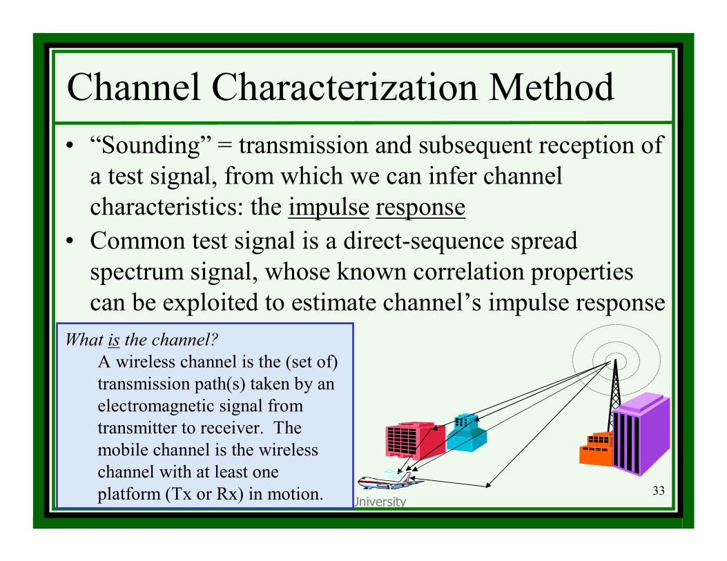
Channel Characterization Method• “Sounding” = transmission and subsequent reception of

a test signal, from which we can infer channel characteristics: the impulse response

• Common test signal is a direct-sequence spread spectrum signal, whose known correlation properties can be exploited to estimate channel’s impulse response

What is the channel?A wireless channel is the (set of) transmission path(s) taken by an electromagnetic signal from transmitter to receiver. The mobile channel is the wireless channel with at least one platform (Tx or Rx) in motion.

Ohio University34

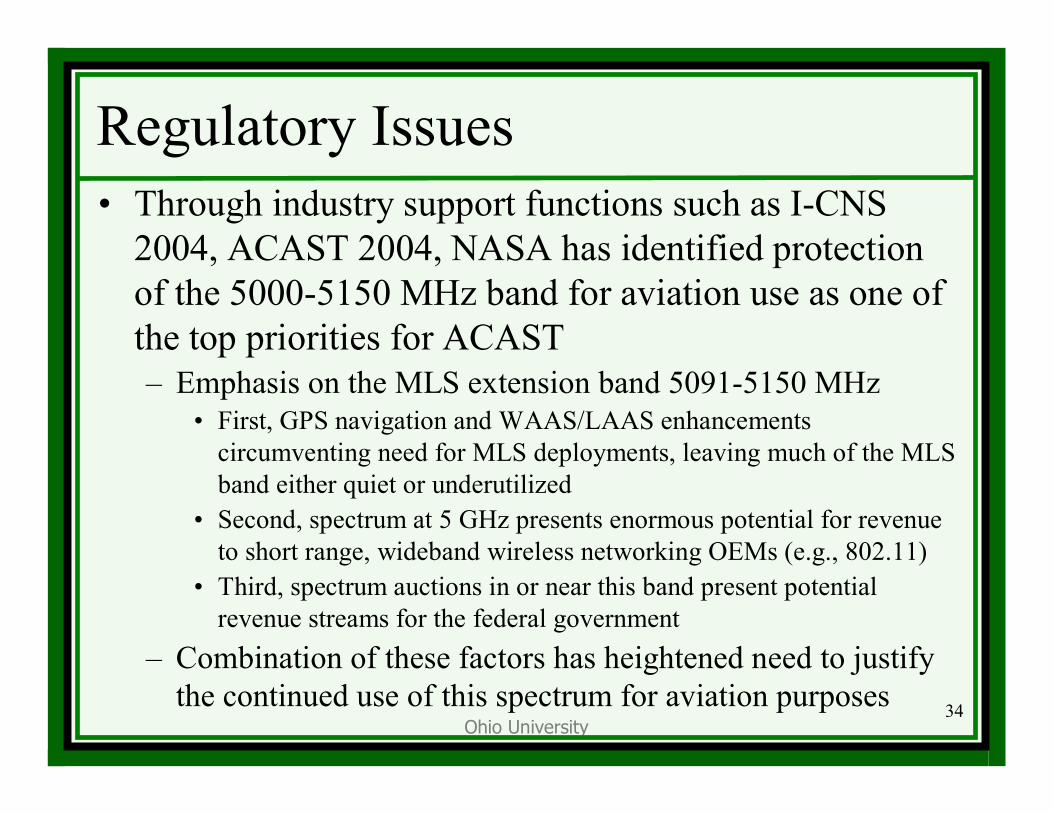
Regulatory Issues• Through industry support functions such as I-CNS

2004, ACAST 2004, NASA has identified protection of the 5000-5150 MHz band for aviation use as one of the top priorities for ACAST– Emphasis on the MLS extension band 5091-5150 MHz

• First, GPS navigation and WAAS/LAAS enhancements circumventing need for MLS deployments, leaving much of the MLS band either quiet or underutilized

• Second, spectrum at 5 GHz presents enormous potential for revenue to short range, wideband wireless networking OEMs (e.g., 802.11)

• Third, spectrum auctions in or near this band present potential revenue streams for the federal government

– Combination of these factors has heightened need to justify the continued use of this spectrum for aviation purposes

Ohio University35

Regulatory Issues (2)• It is NASA’s intent to demonstrate, through ACAST,

the applicability of this band for wideband surface area signaling, and how this usage may alleviate some of the congested VHF voice bands for ATC

• The first step in this effort is proper characterization of the MLS radio channel

• Radio Communication group of the International Telecommunication Union (ITU-R) holds a World Radio Conference (WRC) every 3-4 years – Member nations discuss and decide upon the global use of

radio spectrum at these conferences

Ohio University36

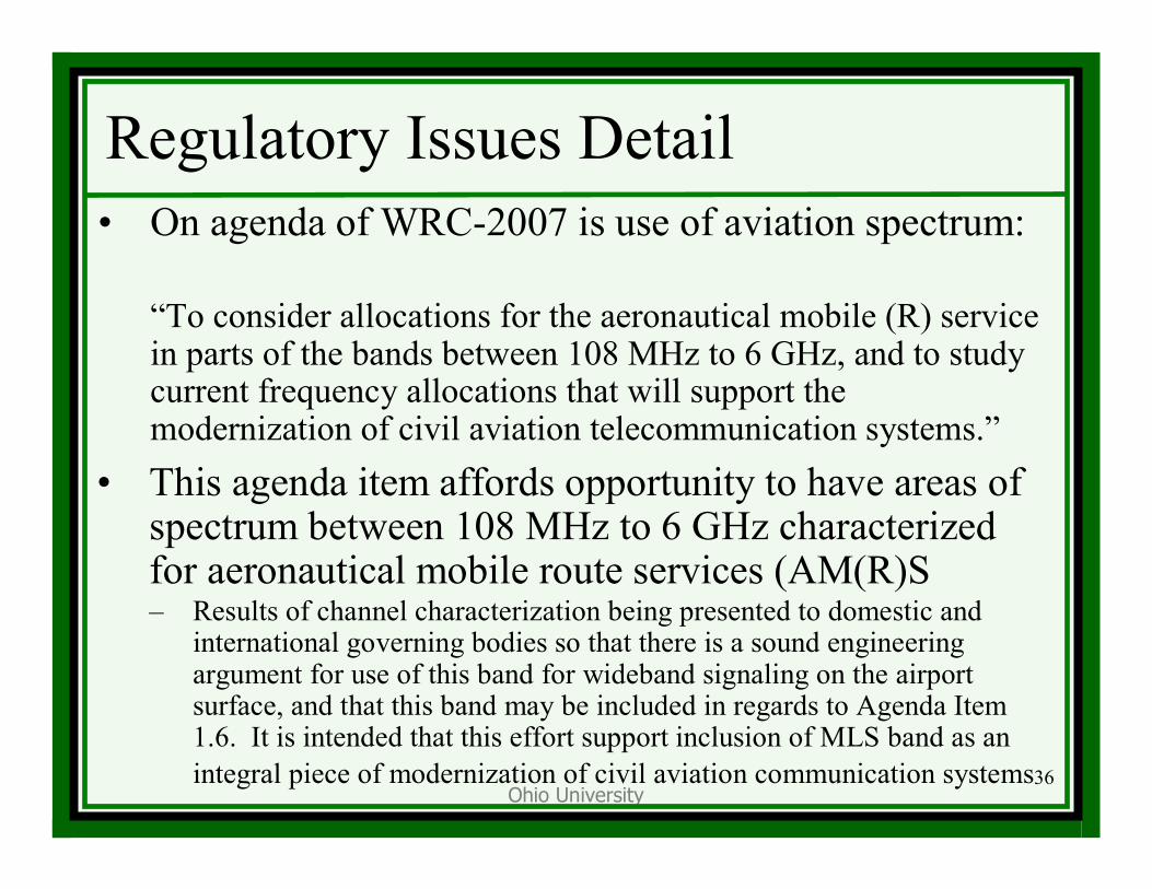
Regulatory Issues Detail• On agenda of WRC-2007 is use of aviation spectrum:

“To consider allocations for the aeronautical mobile (R) service in parts of the bands between 108 MHz to 6 GHz, and to study current frequency allocations that will support the modernization of civil aviation telecommunication systems.”

• This agenda item affords opportunity to have areas of spectrum between 108 MHz to 6 GHz characterized for aeronautical mobile route services (AM(R)S– Results of channel characterization being presented to domestic and

international governing bodies so that there is a sound engineering argument for use of this band for wideband signaling on the airport surface, and that this band may be included in regards to Agenda Item 1.6. It is intended that this effort support inclusion of MLS band as an integral piece of modernization of civil aviation communication systems

Ohio University37

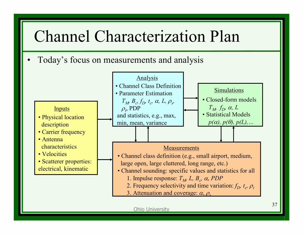
Channel Characterization Plan• Today’s focus on measurements and analysis

Analysis• Channel Class Definition• Parameter Estimation

TM, Bc, fD, tc, α, L, ρs, ρt, PDP

and statistics, e.g., max, min, mean, variance

Simulations• Closed-form models

TM, fD, α, L• Statistical Models

p(α), p(θ), p(L),…

Measurements• Channel class definition (e.g., small airport, medium,

large open, large cluttered, long range, etc.)• Channel sounding: specific values and statistics for all

1. Impulse response: TM, L, Bc, α, PDP2. Frequency selectivity and time variation: fD, tc, ρt3. Attenuation and coverage: α, ρs

Inputs• Physical location

description• Carrier frequency• Antenna

characteristics • Velocities• Scatterer properties: electrical, kinematic

Ohio University38

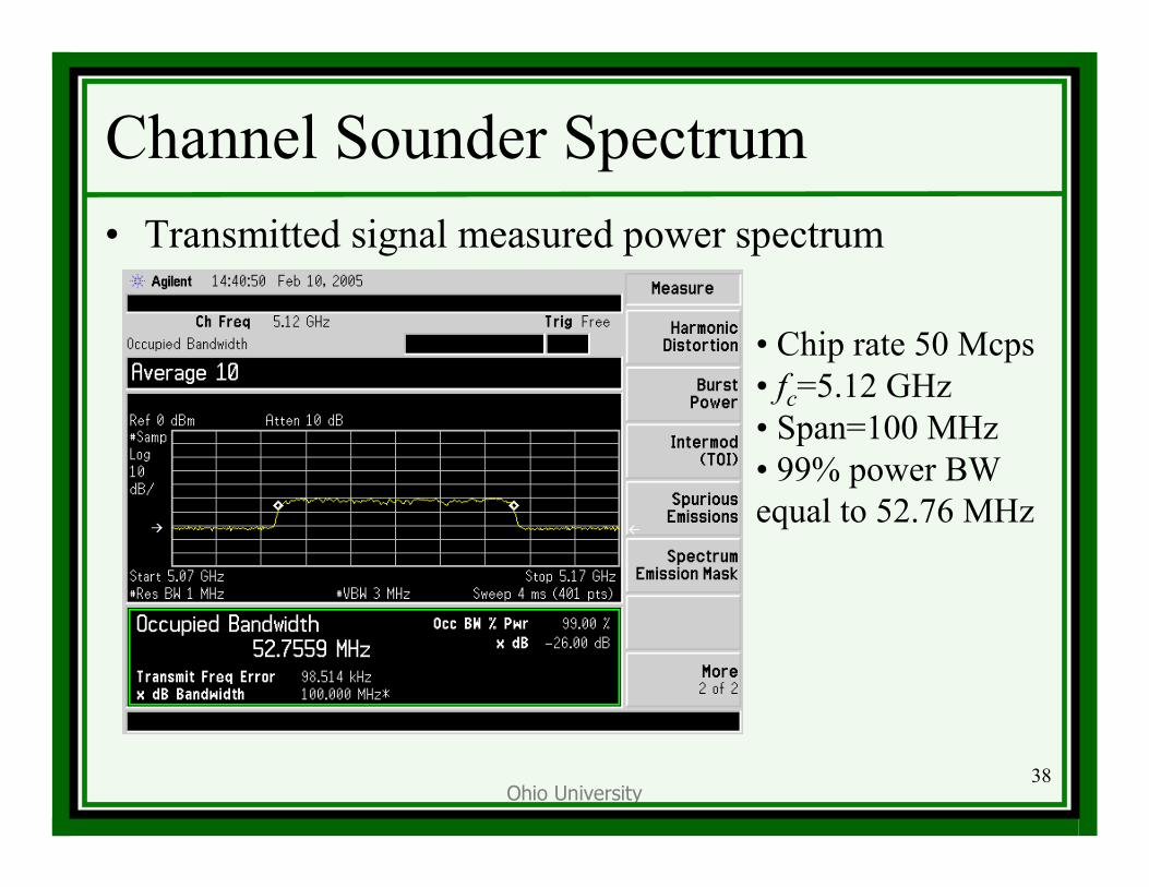
Channel Sounder Spectrum• Transmitted signal measured power spectrum

• Chip rate 50 Mcps• fc=5.12 GHz• Span=100 MHz• 99% power BW equal to 52.76 MHz

Ohio University39

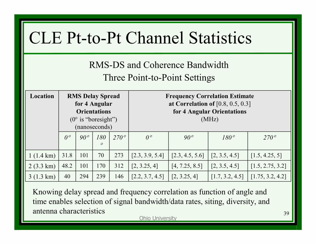
CLE Pt-to-Pt Channel StatisticsRMS-DS and Coherence Bandwidth

Three Point-to-Point Settings

[1.75, 3.2, 4.2][1.7, 3.2, 4.5][2, 3.25, 4][2.2, 3.7, 4.5]146239294403 (1.3 km)

[1.5, 2.75, 3.2][2, 3.5, 4.5][4, 7.25, 8.5][2, 3.25, 4]31217010148.22 (3.3 km)

[1.5, 4.25, 5][2, 3.5, 4.5][2.3, 4.5, 5.6][2.3, 3.9, 5.4]2737010131.81 (1.4 km)

270°180°90°0°270°180°

90°0°

Frequency Correlation Estimateat Correlation of [0.8, 0.5, 0.3]

for 4 Angular Orientations(MHz)

RMS Delay Spread for 4 Angular Orientations

(0° is “boresight”)(nanoseconds)

Location

Knowing delay spread and frequency correlation as function of angle and time enables selection of signal bandwidth/data rates, siting, diversity, and antenna characteristics

Ohio University40

-25-20

-15-10

-50

510

1520

25

00.5

11.5

22.5

33.5-60

-50

-40

-30

-20

-10

0

Rel

ativ

e P

ower

-dB

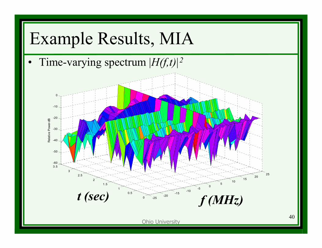
Example Results, MIA• Time-varying spectrum |H(f,t)|2

f (MHz)t (sec)

Ohio University41

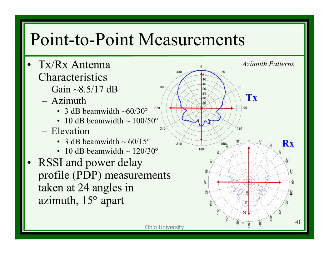
Point-to-Point Measurements• Tx/Rx Antenna

Characteristics– Gain ~8.5/17 dB– Azimuth

• 3 dB beamwidth ~60/30°• 10 dB beamwidth ~ 100/50°

– Elevation • 3 dB beamwidth ~ 60/15°• 10 dB beamwidth ~ 120/30°

• RSSI and power delay profile (PDP) measurements taken at 24 angles in azimuth, 15° apart

Tx

0

15°

30°

45°

60°

75°

90°

105 °

120 °

135 °

150 °

165 °

±180

°

-165

° -150

° -135

°

-120

°-1

05°

-90 °

-75 °

-60 °

-45 °

-30 °-1

5

-60

-40

-20

0

1672

34dB

Rx

-35-30-25-20-15-10-5 0 30

210

60

240

90270

120

300

150

330

180

0Antenna Radiation Pattern for Horn in Azimuth Azimuth Patterns