Mixture of Gaussians Expectation Maximization (EM) Part 1

Mixture of Gaussians

Expectation Maximization (EM)

Part 1

Most of the slides are due to Christopher Bishop

BCS Summer School, Exeter, 2003.

The rest of the slides are based on lecture notes by A. Ng

BCS Summer School, Exeter, 2003 Christopher M. Bishop

Limitations of K-means

• Hard assignments of data points to clusters – small shift

of a data point can flip it to a different cluster

• Not clear how to choose the value of K

• Solution: replace ‘hard’ clustering of K-means with ‘soft’

probabilistic assignments

• Represents the probability distribution of the data as a

Gaussian mixture model


The Gaussian Distribution

• Multivariate Gaussian

• Define precision to be the inverse of the covariance

• In 1-dimension

mean covariance


Gaussian Mixtures

• Linear super-position of Gaussians

• Normalization and positivity require

• Can interpret the mixing coefficients as prior probabilities

)|x()()x(1

K

k

kpkpp

Sampling from the Gaussian

• To generate a data point:

– first pick one of the components with probability

– then draw a sample from that component

• Repeat these two steps for each new data point



Example: Gaussian Mixture Density

• Mixture of 3 Gaussians

xp5.0xp3.0xp2.0)x(p 321

10

01,00N)x(p1

40

04,6,6N)x(p2

60

06,7,7N)x(p3

p1(x)

p2(x)

p3(x)


Synthetic Data Set


Fitting the Gaussian Mixture

• We wish to invert this process – given the data set, find

the corresponding parameters:

– mixing coefficients

– means

– covariances

• If we knew which component generated each data point,

the maximum likelihood solution would involve fitting

each component to the corresponding cluster

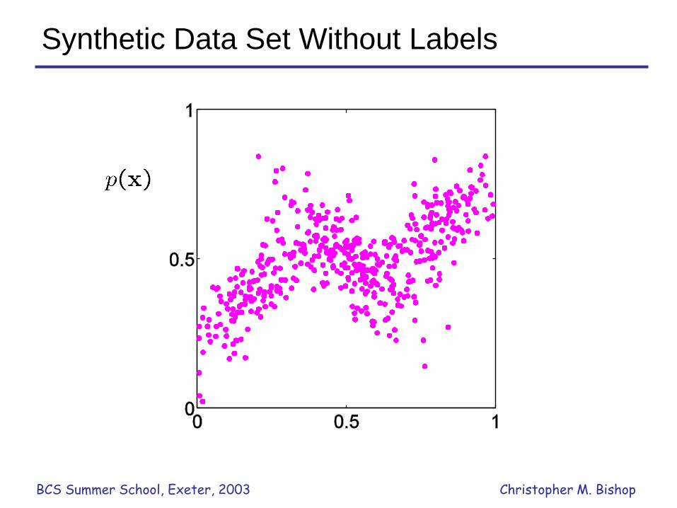
• Problem: the data set is unlabelled

• We shall refer to the labels as latent (= hidden) variables


Synthetic Data Set Without Labels


Posterior Probabilities

• We can think of the mixing coefficients as prior

probabilities for the components

• For a given value of we can evaluate the

corresponding posterior probabilities, called

responsibilities

• These are given from Bayes’ theorem by


Posterior Probabilities (colour coded)

)|( xkp


Posterior Probability Map


Maximum Likelihood for the GMM

• The log likelihood function takes the form

• Note: sum over components appears inside the log

• There is no closed form solution for maximum likelihood

• How to maximize the log likelihood

– solved by expectation-maximization (EM) algorithm


EM Algorithm – Informal Derivation

• Let us proceed by simply differentiating the log likelihood

• Setting derivative with respect to equal to zero gives

giving

which is simply the weighted mean of the data



• Similarly for the covariances

• For mixing coefficients use a Lagrange multiplier to give

Average responsibility which component j takes for

explaining the data points.



• The solutions are not closed form since they are coupled

• Suggests an iterative scheme for solving them:

– Make initial guesses for the parameters

– Alternate between the following two stages:

1. E-step: evaluate responsibilities

2. M-step: update parameters using ML results

Mixture of Gaussians Expectation Maximization (EM) Part 1

Documents

Transcript of Mixture of Gaussians Expectation Maximization (EM) Part 1