Mixed Stabilized Finite Element Methods in...
38
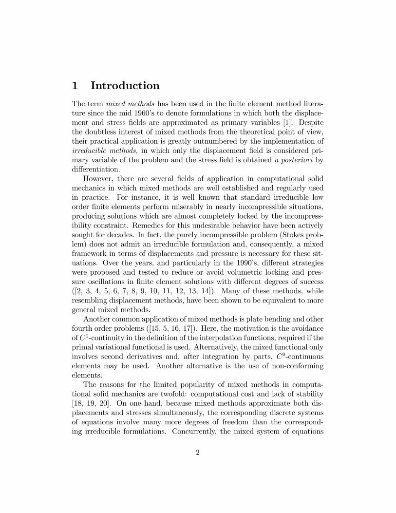
Mixed Stabilized Finite Element Methods in Nonlinear Solid Mechanics. Part I: Formulation M. Cervera, M. Chiumenti and R. Codina International Center for Numerical Methods in Engineering (CIMNE) Technical University of Catalonia (UPC) Edicio C1, Campus Norte, Jordi Girona 1-3, 08034 Barcelona, Spain. Keywords: mixed nite element interpolations, stabilization methods, algebraic sub-grid scales, orthogonal sub-grid scales, nonlinear solid mechanics. Abstract This paper exploits the concept of stabilized nite element methods to formulate stable mixed stress/displacement and strain/displacement nite elements for the solution of nonlinear solid mechanics prob- lems. The di/erent assumptions and approximations used to derive the methods are exposed. The proposed procedure is very general, applicable to 2D and 3D problems. Implementation and computa- tional aspects are also discussed, showing that a robust application of the proposed formulation is feasible. Numerical examples show that the results obtained compare favourably with those obtained with the corresponding irreducible formulation. 1
Transcript of Mixed Stabilized Finite Element Methods in...

Mixed Stabilized Finite Element Methods inNonlinear Solid Mechanics.
Part I: Formulation
M. Cervera, M. Chiumenti and R. CodinaInternational Center for Numerical Methods in Engineering (CIMNE)
Technical University of Catalonia (UPC)
Edi�cio C1, Campus Norte, Jordi Girona 1-3, 08034 Barcelona, Spain.
Keywords: mixed �nite element interpolations, stabilization methods,algebraic sub-grid scales, orthogonal sub-grid scales, nonlinear solid mechanics.
Abstract
This paper exploits the concept of stabilized �nite element methodsto formulate stable mixed stress/displacement and strain/displacement�nite elements for the solution of nonlinear solid mechanics prob-lems. The di¤erent assumptions and approximations used to derivethe methods are exposed. The proposed procedure is very general,applicable to 2D and 3D problems. Implementation and computa-tional aspects are also discussed, showing that a robust application ofthe proposed formulation is feasible. Numerical examples show thatthe results obtained compare favourably with those obtained with thecorresponding irreducible formulation.
1
1 Introduction
The term mixed methods has been used in the �nite element method litera-ture since the mid 1960�s to denote formulations in which both the displace-ment and stress �elds are approximated as primary variables [1]. Despitethe doubtless interest of mixed methods from the theoretical point of view,their practical application is greatly outnumbered by the implementation ofirreducible methods, in which only the displacement �eld is considered pri-mary variable of the problem and the stress �eld is obtained a posteriori bydi¤erentiation.However, there are several �elds of application in computational solid
mechanics in which mixed methods are well established and regularly usedin practice. For instance, it is well known that standard irreducible loworder �nite elements perform miserably in nearly incompressible situations,producing solutions which are almost completely locked by the incompress-ibility constraint. Remedies for this undesirable behavior have been activelysought for decades. In fact, the purely incompressible problem (Stokes prob-lem) does not admit an irreducible formulation and, consequently, a mixedframework in terms of displacements and pressure is necessary for these sit-uations. Over the years, and particularly in the 1990�s, di¤erent strategieswere proposed and tested to reduce or avoid volumetric locking and pres-sure oscillations in �nite element solutions with di¤erent degrees of success([2, 3, 4, 5, 6, 7, 8, 9, 10, 11, 12, 13, 14]). Many of these methods, whileresembling displacement methods, have been shown to be equivalent to moregeneral mixed methods.Another common application of mixed methods is plate bending and other
fourth order problems ([15, 5, 16, 17]). Here, the motivation is the avoidanceof C1-continuity in the de�nition of the interpolation functions, required if theprimal variational functional is used. Alternatively, the mixed functional onlyinvolves second derivatives and, after integration by parts, C0-continuouselements may be used. Another alternative is the use of non-conformingelements.The reasons for the limited popularity of mixed methods in computa-
tional solid mechanics are twofold: computational cost and lack of stability[18, 19, 20]. On one hand, because mixed methods approximate both dis-placements and stresses simultaneously, the corresponding discrete systemsof equations involve many more degrees of freedom than the correspond-ing irreducible formulations. Concurrently, the mixed system of equations
2
is very often inde�nite, which makes most of the direct and iterative solu-tion methods inapplicable. These di¢ culties may be avoided with a suitableimplementation. On the other hand, many choices of the individual inter-polation �elds for the mixed problem yield meaningless, not stable, results.This is due to the strictness of the inf-sup condition [19] when the stan-dard Galerkin �nite element method is applied straightforwardly to mixedelements, as it imposes severe restrictions on the compatibility of the inter-polations used for the displacement and the stress �elds. This di¢ culty, ifnot circumvented, is severely restrictive (see [21] and [22, 23] for the analysisof admissible elements in linear elasticity).In parallel, mixed methods have also been the focus of attention in com-
putational �uid dynamics. In [24] and [25], the variational multiscale (VMS)formulation was proposed as a new way of circumventing the di¢ culties posedby the inf-sup condition. In the case of incompressible problems, the reason-ing behind was not new, as it consisted of modifying the discrete variationalform to attain control on the pressure �eld. The result was the possibility ofusing equal order interpolations for displacements and pressures and to con-struct stable low order elements. Since then, the sub-grid concept underlyingthe VMS approach has been extensively and fruitfully used in �uid dynamics.In [26] and [27], the concept of orthogonal subscale stabilization (OSS) wasintroduced, which leads to well sustained and better performing stabilizationprocedures. The analysis of the formulation can be found in [28] for the lin-earized incompressible Navier-Stokes equations and, in subjects closer to thetopic of this paper, in [29] for the stress-displacement-pressure formulation ofthe Stokes problem (equivalent to the linear elastic incompressible problem)and in [30] for Darcy�s problem.In previous works, the authors have applied stabilized mixed displace-
ment/pressure methods (see [31, 32, 33, 34, 35] and [36]) to the solution ofincompressible J2-plasticity and damage problems with strain localization us-ing linear/linear simplicial elements in 2D and 3D. These procedures lead toa discrete problem which is fully stable, free of pressure oscillations and vol-umetric locking and, thus, results obtained are practically mesh independent.This translates in the achievement of two important goals: (a) the positionand orientation of the localization band is independent of the directional biasof the �nite element mesh and (b) the global post-peak load-de�ection curvesare independent of the size of the elements in the localization band. Similarideas have been used in [37, 38] and [39].In the present work we apply this approach in order to derive stable mixed
3
stress-displacement and strain-displacement formulations using linear/linearinterpolations in triangular elements and bilinear/bilinear interpolations inquadrilateral elements. It is noteworthy that, from the numerical point ofview, the di¢ culties encountered in this problem are very di¤erent to thosefound in incompressible situations, analyzed in previous works. The treat-ment of the incompressible case in the stress/displacement formulation wouldrequire considering the pressure as an additional independent variable andappropriate stabilization techniques (see [29]). The incompressible limit willnot be treated here, and the following formulation is limited to compressiblenonlinear solid mechanics.The basic motivation for this work is to show that the di¢ culties en-
countered when solving solid mechanics problems involving the creation andpropagation of strain localization bands using standard elements and localconstitutive models are due to the approximation error inherent to the spatialdiscretization, as well as to the poor stability in the stresses and/or strains.When using the basic, irreducible, formulation of the problem, the stresses(or strains), which are the variables of most interest for the satisfaction of thehighly nonlinear constitutive behavior, are not the fundamental unknownsof the problem and they are obtained by di¤erentiation of the displacement�eld, a process which entails an important loss of accuracy, particularly wherestrong displacement gradients occur. The local approximation error commit-ted makes propagation of the localization bands strongly dependent on the�nite element mesh used. Contrariwise, when using a mixed formulation inwhich the stress (or the strain) �eld is selected as primary variable, togetherwith the displacement �eld, the added accuracy and stability achieved areenough to overcome the mesh dependency problem satisfactorily.The outline of the present paper is as follows. In Section 2 the mixed
stress/displacement �nite element formulation for linear elasticity is sum-marized. The sub-grid scale approach is used to derive two stabilized for-mulations. Results concerning stability and convergence of these schemesare discussed. In Section 3 the stabilization is extended to nonlinear prob-lems, proposing both stress-displacement and strain-displacement formula-tions. The later can be considered more suitable for the implementation ofnonlinear constitutive models. Implementation and computational aspectsare discussed next. Finally, some numerical benchmarks and examples arepresented to assess the present formulation and to compare its performancewith the standard irreducible elements. The problem of strain localization isdiscussed in a companion paper [36].
4
2 Mixed stabilized stress�displacement for-mulation in linear elasticity
2.1 Continuous problem
The formulation of the solid mechanics problem can be written consideringthe stress as an independent unknown, additional to the displacement �eld.In this case, the strong form of the continuous problem can be stated as:given a �eld of prescribed body forces f and a constant constitutive tensorC, �nd the displacement �eld u and the stress �eld � such that:
�� +C : rsu = 0 in (1a)
r � � + f = 0 in (1b)
where is the open and bounded domain of Rndim occupied by the solid ina space of ndim dimensions.Equations (1a)-(1b) are subjected to appropriate Dirichlet and Neumann
boundary conditions. In the following, we will assume these, without lossof generality, in the form of prescribed displacements u = 0 on @u, andprescribed tractions t on @t, respectively, being @u and @t a partition [email protected] by the test functions and integrating by parts the second
equation, the associated weak form of the problem (1a)-(1b) can be statedas:
��� ;C�1 : �
�+ (� ;rsu) = 0 8� (2a)
(rsv;�) = (v; f) +�v; t�@t
8v (2b)
where v 2 V and � 2 T are the test functions of the displacement and stress�elds, respectively, and (�; �) denotes the inner product in L2 (), the space ofsquare integrable functions in . Hereafter, orthogonality will be understoodwith respect to this product. Likewise, (v;�t)@t denotes the integral of vand �t over @t. For the sake of shortness, we will write F (v) = (v; f) +�v; t�@t
in the following. Equations (2a)-(2b) can be understood as thestationary conditions of the classical Hellinger-Reissner functional (see [41]for a description of a broader class of mixed methods).The space of stresses T consists of symmetric tensors whose components
are in L2(). If the weak form is written as indicated in (2a), the displace-ments and their test functions have to have components in H1 () (they and
5
their derivatives have to be in L2()) and must vanish on @u. This de�nesthe space of displacements V. However, it is also possible to integrate the sec-ond term in (2a) by parts, obtaining (� ;rsu) = �(r�� ;u), and similarly forthe left-hand-side of (2b). In this case, the components of the stresses haveto have also the divergence in L2(), but the components of the displacementneed to be only in L2(), not H1(). Similarly to Darcy�s problem, thereare two possible functional settings for the linear elastic problem written inmixed form (see [30]). This is not essential for our discussion, although ithas some implications in the treatment of boundary conditions on which wewill not enter.
2.2 Galerkin �nite element approximation
Let us now de�ne the discrete Galerkin �nite element counterpart problemas:
��� h;C
�1 : �h�+ (� h;rsuh) = 0 8� h (3a)
(rsvh;�h) = F (vh) 8vh (3b)
where uh ; vh 2 Vh and �h ; � h 2 Th are the discrete displacement andstress �elds and their test functions, de�ned onto the �nite element spaces Vhand Th, respectively. Note that the resulting system of equations is symmetricbut non-de�nite. In all what follows, we will be interested in continuous�nite element spaces Vh and Th and, more speci�cally, in equal interpolationfor stresses and displacements. Therefore, we may replace (� h;rsvh) by�(r � � h;vh), for all vh 2 Vh and � h 2 Th.As it is well known, the stability of the discrete formulation depends
on appropriate compatibility restrictions on the choice of the �nite elementspaces Vh and Th, as stated by the inf-sup condition [19]. According to this,standard Galerkin mixed elements with continuous equal order linear/linearinterpolation for both �elds are not stable. Lack of stability shows as un-controllable oscillations in the displacement �eld that entirely pollute thesolution. Fortunately, the strictness of the inf-sup condition can be avoidedby modifying the discrete variational form, for instance, by means of in-troducing appropriate numerical techniques that can provide the necessarystability to the desired choice of interpolation spaces. The objective of thiswork is precisely to present stabilization methods which allow the use of equalorder continuous interpolations for displacements and stresses.
6
2.3 Stabilized �nite element methods
2.3.1 Scale splitting
The basic idea of the sub-grid scale approach [24] is to consider that thecontinuous unknowns can be split in two components, one coarse and a �nerone, corresponding to di¤erent scales or levels of resolution. The solution ofthe continuous problem contains components from both scales.For the solution of the discrete problem to be stable it is necessary to,
somehow, include the e¤ect of both scales in the approximation. The coarsescale can be appropriately solved by a standard �nite element interpolation,which however cannot solve the �ner scale. Nevertheless, the e¤ect of this�ner scale can be included, at least locally, to enhance the stability of thedisplacement in the mixed formulation.To this end, the stress and the displacement �elds of the mixed problem
will be approximated as
� = �h + e�; u = uh + eu (4)
where �h 2 Th and uh 2 Vh are the components of the stresses and thedisplacements on the (coarse) �nite element scale and e� 2 eT and eu 2 eV arethe enhancement of the stresses and the displacements corresponding to the(�ner) sub-grid scales. Let us also consider the corresponding test functionse� 2 eT and ev 2 eV. This approximation extends the stress solution spaceto T ' Th � eT , and the displacement solution space to V ' Vh � eV. Eachparticular stabilized �nite element method is de�ned according to the wayin which spaces eT and eV are chosen. In particular, the Galerkin methodcorresponds to taking eT = f0g, eV = f0g.As it has been mentioned, in what follows we will consider continuous
�nite element interpolations. Likewise, we will assume that the subscalesvanish on the interelement boundaries. When more general situations areconsidered, additional terms involving interelement boundary integrals needto be added (see [30, 42]).Introducing the splitting, the problem corresponding to (2a)-(2b) is:
��� h;C
�1 : �h���� h;C
�1 : e��+ (� h;rsuh)� (r � � h;eu) = 0 8� h (5a)
��e� ;C�1 : �h
���e� ;C�1 : e��+ (e� ;rsuh) + (e� ;rseu) = 0 8e� (5b)
(rsvh;�h) + (rsvh; e�) = F (vh) 8vh (5c)
� (ev;r � �h)� (ev;r � e�) = F (ev) 8ev (5d)
7
where some terms have been integrated by parts and we have assumed thateu and ev vanish on the boundary. In the following, the fact that the discretevariational equations need to hold for all test functions will be omitted.Due to the approximation used, (4), and the linear independence of � h
and e� , now the continuous equation (2a) unfolds in two discrete equations,(5a) and (5b), one related to each scale considered. The same comment isapplicable to the displacement splitting. Equations (5a) and (5c) are de�nedin the �nite element spaces Th and Vh; respectively. The �rst one enforces theconstitutive equation including a stabilization term S1 = �
�� h;C
�1 : e�� �(r � � h;eu) depending on the sub-grid stresses and displacements. The secondone solves the balance of momentum including a stabilization term S2 =(rsvh; e�) depending on the sub-grid stresses e�:Let us de�ne the residuals of the �nite element components as
r�;h = C�1 : �h �rsuh (6a)
ru;h = f +r � �h (6b)
These allow us to write (5b) and (5d) as
��e� ;C�1 : e��+ (e� ;rseu) = (e� ; r�;h) (7a)
� (ev;r � e�) = (ev; ru;h) (7b)
These equations are the projections of the �nite element residuals onto thespace of sub-scales, which cannot be resolved by the �nite element mesh.Therefore, to proceed it is necessary to provide an approximate closed formsolution to them. If eP� and ePu are the projections onto eT and eV, respectively,note �rst that we may write (7a) and (7b) as
eP�(�C�1 : e� +rseu) = eP�(r�;h) (8a)ePu(�r � e�) = ePu(ru;h) (8b)
and therefore the problem is to approximate the operators on the left-hand-side of these equations. The way we motivate such an approximation is byusing an approximate Fourier analysis of the problem. Using exactly the sameprocedure as in [43], it can be shown that e� and eu may be approximatedwithin each element by
e� = ���C : eP�(r�;h) = �� eP�(C : rsuh � �h) (9a)eu = �u ePu(ru;h) = �u ePu(f +r � �h) (9b)
8
where the so called stabilization parameters �� and �u can be computed as
�� = c�h
L0; �u = cu
L0h
Cmin(10)
and where c� and cu are algorithmic constants, L0 is a characteristic length ofthe computational domain, h is the element size and Cmin > 0 is the smallesteigenvalue of C (see below). As shown in [30], this is the choice of the para-meters that yields best order of convergence for equal order of interpolationof stresses and displacements. In the following, and for the sake of clarity,we will consider the mesh quasi-uniform, so that a unique h can be de�nedfor all the mesh, and thus �� and �u will be constant. In general situations,it is understood that these parameters have to be evaluated elementwise.The methods we wish to consider are completely de�ned up to the choice
of the projections eP� and ePu. Two possible options are described next.2.3.2 Residual based algebraic subgrid scale method
The simplest choice is to take eP� and ePu as the identity when applied to theresiduals in (9a) and (9b). In fact, one may also think that the projection isscaled by the stabilization parameters given by (10), which act as upscalingof the residuals onto the �nite element mesh. This is what is called algebraicsubgrid scale (ASGS) method in [30], for example. If the subscales resultingfrom these equations are then inserted into (5a) and (5c) one gets
� (1� ��)�� h;C
�1 : �h�+ (1� ��) (� h;rsuh)� �u(r � � h;r � �h) = �u(r � � h; f) (11a)(1� ��) (rsvh;�h) + �� (rsvh;C : rsuh) = F (vh) (11b)
Note that the resulting system of equations is symmetric.Particularly interesting is the case �u = 0. In this situation, (11a) repre-
sents a projection onto the discrete �nite element space that can be writtenas
�h = Ph (C : rsuh) (12)
and, therefore, the discrete balance equation (11b) takes the form:
(1� ��) (rsvh;Ph (C : rsuh)) + �� (rsvh;C : rsuh) = (vh; f)
Thus, for �u = 0 the method we propose can be rewritten as
�stab = (1� ��)Ph (C : rsuh) + �� (C : rsuh) (13a)
(rsvh; �stab) = F (vh) (13b)
9
This compact form of writing the problem is only possible when �u = 0:Otherwise, (11a)-(11b) have to be kept as such.Some remarks are in order:
1. The stabilization term S2 in (5c) is computed in an element by el-ement manner and within each element. Its magnitude depends onthe di¤erence between the continuous (projected) stresses �h and thediscontinuous (elemental) stresses C : rsuh:
2. This means that the term added to secure a stable solution decreasesupon mesh re�nement, as the �nite element scale becomes �ner andthe residual reduces.
3. In other words, e� is �small�compared to �h.4. With this de�nition, e� is discontinuous across element boundaries. Forlinear elements, e� is piece-wise linear.
5. Even if de�ned element-wise, e� cannot be condensed at the elementlevel, because �h is interelement continuous.
6. In the localization process in (9a), it is necessary to neglect the integralsover element faces involving the sub-scale, in front of the integrals overthe element volumes. This is justi�ed in [44] resorting to Fourier analy-sis and recalling that the subscale is associated to frequencies higherthan the grid scale. It is worth to mention that for �bubble�-type en-hancements these boundary terms are null by construction [45, 46]. Seealso [42] for a possible generalization.
7. Equation (9a) must not be interpreted point-wise, as the values of e�are not used in the stabilization procedure; only the integrals S1 andS2 in (5a)-(5c) are needed.
2.3.3 Orthogonal subscale stabilization
It was argued in [27] that a very natural choice for the unknown subgridspaces is to take them orthogonal to the �nite element space. This amountsto saying that the projections eP� and ePu are taken as P?h applied to theappropriate space of discrete functions. This also means approximating thestress solution space as T ' Th�T ?h and, similarly, the displacement solution
10
space as V ' Vh�V?h . The subsequent stabilization method is called orthogo-nal subscale stabilization (OSS) method, and it has already been successfullyapplied to several problems in �uid and solid mechanics.Noting that �h is a �nite element function and computing P?h = I � Ph
(I being the identity), the subscales can be now expressed as
e� = ��P?h (C : rsuh) = �� [C : rsuh � Ph(C : rsuh)] (14a)eu = �uP?h (f +r � �h) = �u [f +r � �h � Ph(f +r � �h)] (14b)
Introducing these orthogonal subscales in (5a) and (5c) the �rst componentin the stabilization term S1 vanishes because of orthogonality and the mixedsystem of equations can be written as
��� h;C
�1 : �h�+ (� h;rsuh)� �u(r � � h; P?h (r � �h)) = �u(r � � h; P?h (f)) (15a)(rsvh;�h) + ��(rsvh; P
?h (C : rsuh)) = F (vh) (15b)
It is also interesting to consider the case �u = 0. Now (15a) is identicalto (11a) in the previous Section and, therefore, it can be written as (12) onceagain. With this de�nition, the orthogonal subscale in (14a) is identical tothe residual-based subscale in (9a) with eP� = I. Therefore, the resultingstabilization terms are also identical and the system of equations (15a)-(15b)can be arranged as in system (11a)-(11b) or system (13a)-(13b). Therefore,when �u = 0 the ASGS and the OSS formulations coincide.
2.4 Stability and convergence results
In this section we state stability and convergence results both for the OSSmethod given by (15a)-(15b) and for the ASGS method given by (11a)-(11b),which, as we have seen, coincide when �u = 0. The proof of these results canbe done adapting the analysis presented in [30]. To simplify the exposition,we will consider the boundary tractions t = 0.The constitutive tensor C is assumed to be constant, symmetric and
positive de�nite. Let Cmax > 0 and Cmin > 0 be such that
Cmin : � : C : � Cmax :
for all symmetric second order tensors .
11

Let k � k denote the standard norm in L2(). For the continuous problem(2a)-(2b) it can be shown that
1
Cmaxk�k2 + L20
Cmaxkr � �k2 + Cmin
L20kuk2 + Cminkrsuk2 . L20
Cminkfk2 (16)
This result gives optimal stability in all the �elds involved in the problem.The symbol . is used to include constants independent of the unknowns andthe components of C (and of h, in what follows).For the Galerkin �nite element approximation to the problem, a bound
similar to (16) can be proved provided the appropriate inf-sup conditions be-tween the interpolating spaces are met. Moreover, in general it is not possibleto bound both kr � �hk2 and krsuhk2, but only one of these two terms.Stabilized �nite element methods aim precisely at providing stability es-
timates without relying on compatibility conditions. In particular, for themethods given by (11a)-(11b) and by (15a)-(15b) it can be shown that
1
Cmaxk�hk2+
L0h
Cmaxkr��hk2+
CminL20
kuhk2+Cminh
L0krsuhk2 .
L20Cmin
kfk2 (17)
where the divergence of the stresses in the left-hand-side has to be dropped if�u = 0. This estimate resembles very much (16) for the continuous problem.The only di¤erence is the factor h instead of L0 in two terms of the left-hand-side. This however does not prevent from obtaining the error estimates
1
Cmaxk� � �hk2 +
L0h
Cmaxkr � (� � �h)k2 +
+CminL20
ku� uhk2 +Cminh
L0krs(u� uh)k2
. L0Cmin
h2k+1j�j2k+1 +CmaxL0
h2k+1juj2k+1 (18)
when interpolations of degree k are used for both the stresses and the dis-placements.The symbol j � jk+1 denotes the L2() norm of the derivatives of order
k + 1 of the unknowns, which have been assumed su¢ ciently regular.The L2() estimates given in (18) can be improved using duality argu-
ments. The analysis in [30] can be adapted to obtain
k� � �hk . hkr � (� � �h)k+ Cmaxh
L0krs(u� uh)k (19)
ku� uhk . L0h
Cminkr � (� � �h)k+ hkrs(u� uh)k (20)
12
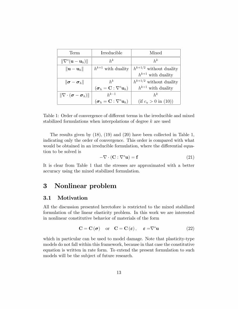
Term Irreducible Mixed
krs(u� uh)k hk hk
ku� uhk hk+1 with duality hk+1=2 without dualityhk+1 with duality
k� � �hk hk hk+1=2 without duality(�h = C : rsuh) hk+1 with duality
kr � (� � �h)k hk�1 hk
(�h = C : rsuh) (if cu > 0 in (10))
Table 1: Order of convergence of di¤erent terms in the irreducible and mixedstabilized formulations when interpolations of degree k are used
The results given by (18), (19) and (20) have been collected in Table 1,indicating only the order of convergence. This order is compared with whatwould be obtained in an irreducible formulation, where the di¤erential equa-tion to be solved is
�r � (C : rsu) = f (21)
It is clear from Table 1 that the stresses are approximated with a betteraccuracy using the mixed stabilized formulation.
3 Nonlinear problem
3.1 Motivation
All the discussion presented heretofore is restricted to the mixed stabilizedformulation of the linear elasticity problem. In this work we are interestedin nonlinear constitutive behavior of materials of the form
C = C (�) or C = C (") ; " =rsu (22)
which in particular can be used to model damage. Note that plasticity-typemodels do not fall within this framework, because in that case the constitutiveequation is written in rate form. To extend the present formulation to suchmodels will be the subject of future research.
13

The misbehavior encountered when irreducible formulations are used iswell known, and has been described already in Section 1. The numericalproblems found can be attributed to poor stability and/or accuracy in thecomputation of the stresses. Since they are used to evaluate the constitutivelaw (22), it is not surprising that a failure in calculating the stresses leads toa global failure of the overall numerical approximation.Our proposal in this work is simple: numerical instabilities present in non-
linear solid mechanics using the irreducible formulation (i.e., approximating(21)) could be at least alleviated if stability and/or accuracy in the calcu-lation of the stresses are improved. And this improvement can be achievedby using a mixed formulation. However, the price to be paid is to use in-terpolations for the stresses and the displacements that satisfy the inf-supcompatibility condition, and this very often leads to non-standard (if notdirectly exotic) interpolating pairs. The tool to overcome this is to resort tostabilized formulations, as we have shown so far.Even though we do not have the analysis for nonlinear problems, the
results presented in Section ?? suggest that success is possible. In particular:
� Stress stability is improved. From estimate (17) it is observed thatin the linear case stress stability is obtained without relying on thestability obtained for the displacement �eld.
� Stress accuracy is improved, as it is clearly seen from Table 1 in linearelasticity. As a particular case, consider k = 1 (linear interpolation).In the irreducible formulation the stresses are approximated with orderh in the L2() norm. Without additional conditions on the regular-ity of the solution and the shape of the elements of the �nite elementmesh, pointwise estimates are expected to have one order less of conver-gence. This means that no convergence order can be guaranteed for thestresses that are used to evaluate the constitutive law (22) pointwise.For the mixed stabilized formulation we can formally expect order hconvergence in the worst situation (order h1=2 if the assumptions ofduality arguments do not apply).
In the following we describe how to formulate mixed stabilized methodsin the nonlinear case. The �rst point to keep in mind is that results will bedi¤erent depending on whether stresses or strains are used as independentvariables to be interpolated. In the linear case there is obviously no di¤erence,
14
since for constant constitutive tensors C the space for the discrete strains"h = C�1 : �h is the same as the space for the discrete stresses �h, andformulating the mixed methods presented in Section ?? in strains is trivial.
3.2 Stress/displacement formulation
For the sake of conciseness, in this subsection we assume that eu = 0. In-cluding displacement subscales in the following discussion is straightforward.The only remarks to be made are that the ASGS and the OSS methods willnot yield the same methods, as we have seen, and stability and convergencefor the divergence of the stresses will be lost if eu = 0.3.2.1 General formulation
Introducing the scale splitting as described in Subsection ?? we arrive atproblem (5a)-(5d) also in the nonlinear case. In the case eu = 0; we mayrewrite this problem as
��� h;C
�1 : �h���� h;C
�1 : e��+ (� h;rsuh) = 0 (23a)
(rsvh;�h) + (rsvh; e�) = (vh; f) (23b)
� eP�(C�1 : e�) = eP�(C�1 : �h)� eP�(rsuh) (23c)
where (23c) corresponds to (8a). Let us see how to particularize this generalframework to the ASGS and the OSS methods.
ASGS method In this case eP� = I when applied to the residual scaledby ��, and we may approximate
e� = ��(C : rsuh � �h) (24)
Note that if �� 6= 1 then e�+�h 6= C : rsuh. As it has been mentioned pre-viously, the scaling of the residual by �� can be understood as the upscalingof e� to the �nite element mesh.From (23a)-(23c) and (24) it follows that (11a)-(11b) is still valid in the
nonlinear case, that is to say,
��� h;C
�1 : �h�+ (� h;rsuh) = 0 (25a)
(1� ��) (rsvh;�h) + �� (rsvh;C : ruh) = (vh; f) (25b)
15
Even though the discrete problem is already given by (25a)-(25b), it issuggestive to write it in a form similar to (13a)-(13b). Let PC�1 denote theL2() projection onto the �nite element space of stresses weighted by C�1.Since (� h;rsuh) = (� h;C
�1 : C : rsuh), we may write (25a) as
�h = PC�1(C : rsuh) (26)
from where it follows that, similarly to (13a)-(13b), the ASGS formulationcan be expressed as
�stab = (1� ��)PC�1 (C : rsuh) + �� (C : rsuh) (27a)
(rsvh; �stab) = F (vh) (27b)
Clearly, for constant constitutive tensors C there is no di¤erence between(27a)-(27b) and (13a)-(13b), but the weighted L2() projection should be inprinciple taken into account in nonlinear constitutive models or simply whenthe medium is not homogeneous.
OSS method The �rst option would be to take eP� = P?h . In this case,(23c) becomes
�P?h (C�1 : e�) = P?h (C�1 : �h)� P?h (rsuh) (28)
However, it is not computationally simple to obtain an expression for thesubgrid stresses from this equation. To construct a basis for the orthogonalto the space of stresses is required to invert the left-hand-side. A simplerand perhaps more natural option is to take eT orthogonal to Th with respectto PC�1. From (23c) it immediately follows that
e� = ��P?C�1(C : rsuh) (29)
and, as for the linear elasticity problem, it can be shown that the OSS andthe ASGS formulations coincide and are given by (27a)-(27b).
3.2.2 Simpli�cations
System (27a)-(27b) can be approximated as is, but there are two approxima-tions that simplify its numerical implementation:
16
� C (�) � C (�h). Even though we have not explicitly indicated it ear-lier, the dependence of C on the stresses needs to be approximated.One possibility is to use �stab given by (27a)-(27b), although, since thesubscales are expected to be much smaller than the �nite element scales,C can be evaluated also with �h. This simpli�es the implementationwhen the displacement subscales are accounted for (see (11a)-(11b)).
� PC�1 � Ph. At the computational level, it is much easier to deal withthe standard L2() projection than with the weighted one. In particu-lar, simpler numerical integration rules may be used. Likewise, lumpingof the matrix resulting from the projection is possible.
3.3 Strain/displacement formulation
3.3.1 General formulation
The formulation of the mixed solid mechanics problem in terms of the stressand displacement �elds, �=u, is classical and it has been used many times inthe context of linear elasticity, where the constitutive tensor C is constant.However, it is not the most convenient format for the nonlinear problem. Thereason for this is that most of the algorithms used for nonlinear constitutiveequations in solid mechanics have been derived for the irreducible formula-tion. This means that these procedures are usually strain driven, and theyhave a format in which the stress � is computed in terms of the strain ",with " =rsu:Therefore, in order to be able to use the existing technology available for
the integration of nonlinear constitutive equations, it is convenient to derivea mixed strain/displacement, "=u; stabilized formulation for the nonlinearsolid mechanics problem. In view of the previous developments this is easilyaccomplished.In this case, the strong form of the continuous problem can be stated
as: for given prescribed body forces f ; �nd the displacement �eld u and thestrain �eld " such that:
�C : "+C : rsu = 0 in (30a)
r � (C : ") + f = 0 in (30b)
Equation (30a) represents strain compatibility, while (30b) is the Cauchyequation. Equations (30a)-(30b) are subjected to appropriate Dirichlet andNeumann boundary conditions.
17
If V is, as before, the space of displacements and G the space of strains,following the standard procedure the associated weak form of the problem(30a)-(30b) can be stated as:
� ( ;C : ") + ( ;C : rsu) = 0 8 (31a)
(rsv;C : ") = (v; f) 8v (31b)
where v 2 V and 2 G are the test functions of the displacements andstrain �elds, respectively. Equations (30a)-(30b) can be understood as thestationary conditions of the classical (reduced) Hu-Washizu functional [41].The discrete Galerkin �nite element counterpart problem is:
� ( h;C : "h) + ( h;C :rsuh) = 0 8 h (32a)
(rsvh;C : "h) = F (vh) 8vh (32b)
where uh ; vh 2 Vh and "h ; h 2 Gh are the discrete displacement andstrain �elds and their test functions, de�ned onto the �nite element spaces Vhand Gh, respectively. Note that the resulting system of equations is symmetricbut non-de�nite.Stability considerations for the mixed "=u are analogous to those of the
�=u format, so we proceed to present a stabilization method, using theresidual-based sub-grid scale approach, which allows in particular the useof linear/linear interpolations for displacements and strains. To this end, thestrain �eld of the mixed problem is approximated as
" = "h + e" (33)
where "h 2 Gh is the strain component of the (coarse) �nite element scale ande" 2 eG is the enhancement of the strain �eld corresponding to the (�ner) sub-grid scale. Let us also consider the corresponding test functions h 2 Gh ande 2 eG, respectively. The strain solution space is G ' Gh � eG: For simplicity,no subscale will be considered for the displacement �eld for the moment. Itsinclusion is considered in subsection 3.4.. Thus, considering only the strainsubscale, the discrete problem corresponding to (31a) and (31b) is now:
� ( h;C : "h)� ( h;C : e") + ( h;C :rsuh) = 0 8 h (34a)
� (e ;C : "h)� (e ;C : e") + (e ;C :rsuh) = 0 8e (34b)
(rsvh;C : "h) + (rsvh; C : e") = F (vh) 8vh (34c)
18
As for the stress-displacement approach, the fact that the discrete variationalequations need to hold for all test functions will be omitted in the following.Due to the approximation used in (33), and the linear independence of
"h and e", the continuous equation (31a) unfolds in two discrete equations,(34a) and (34b), one related to each scale considered. Equations (34a) and(34c) are de�ned in the �nite element spaces Gh and Vh; respectively. The�rst one enforces the constitutive equation including a stabilization termS1 = ( h; C : e") depending on the sub-grid strains e": The second one solvesthe balance of momentum including a stabilization term S2 = (rsvh; C : e")depending on the sub-grid stresses e� = C : e": On the other hand, equation(34b) is de�ned in the sub-grid scale space eG and, hence, it cannot be solvedby the �nite element mesh.Following the same arguments introduced in the previous Section, we can
write (34b) as� (e ; C : e") = (e ; rh) (35)
where the residual of the constitutive equation in the �nite element scale isde�ned as:
rh = rh ("h;uh) = C : "h �C :rsuh (36)
In the case of the residual based ASGS formulation, the sub-scale straincan be localized within each �nite element, and be expressed as
e" = � "C�1 : rh = � " [rsuh � "h] (37)
where � " is computed in terms of an algorithmic constant c" as
� " = c"h
L0(38)
Introducing the strain subscale (37) in (34a) the mixed system of equa-tions can be written as
� (1� � ") ( h;C : "h) + (1� � ") ( h;C :rsuh) = 0 (39a)
(1� � ") (rsvh;C : "h) + � " (rsvh; C : rsuh) = F(vh) (39b)
where the terms depending on � " represent the stabilization. Note that theresulting system of equations is symmetric.If PC is the L2() projection weighted by C, the projection involved in
(39a) can be written as"h = PC (rsuh) (40)
19
and, therefore, the weak form of the balance equation (39b), can be �nallywritten as:
(1� � ") (rsvh;C : PC (rsuh)) + � " (rsvh;C : rsuh) = F(vh) (41)
Equation (37) does not need to be interpreted point-wise, as the valuesof e" are not used in the stabilization procedure; only the integral S2 in (34c)is needed.Similarly to the stress-displacement formulation (27a)-(27b), we can �-
nally write the method we propose for the strain-displacement approach as
"stab = (1� � ")PC (rsuh) + � " (rsuh) (42a)
(rsvh; C : "stab) = F (vh) (42b)
This approach is of straight-forward implementation.As in the previous Section, some remarks are relevant:
1. The stabilization term S2 is computed in an element by element man-ner and, within each element, its magnitude depends on the di¤erencebetween the continuous (projected) and the discontinuous (elemental)strain �elds. This means that the term added to secure a stable solutiondecreases upon mesh re�nement, as the �nite element scale becomes�ner and the residual (or the projection of the residual) reduces ( e" is�small�compared to "h).
2. With the de�nition in (37), the subscale e" is discontinuous across ele-ment boundaries. For linear elements, e" is piece-wise linear. Therefore,even if de�ned element-wise, e" cannot be condensed at element level,because "h is interelement continuous.
The OSS formulation can be developed using the same reasoning as forthe stress-displacement approach. In this case, it is easy to show that if thestrain subscale is taken orthogonal to the �nite element space with respect tothe L2() inner product weighted by C, the resulting formulation is identicalto the ASGS method. Details of the derivation are omitted.
3.3.2 Simpli�cations
Analogously to the stress-displacement formulation, system (42a)-(42b) canbe approximated as is, but there are two approximations that simplify theimplementation:
20
� C(") � C("h).
� PC � Ph.The same remarks as for the stress-displacement formulation are applica-
ble to these approximations.
3.4 Comparison between the �=u and the "=u formu-lations and �nal numerical schemes
As it has been mentioned, the stress-displacement and the strain-displacementformulations will lead to (slightly) di¤erent results in the nonlinear case. Ifwe assume in both cases that �h = C : "h, we have obtained
Stress-displacement: �h = PC�1(C : ruh); "h = C�1 : PC�1(C : ruh)
Strain-displacement: �h = C : PC(ruh); "h = PC(ruh)and for the simpli�ed formulations:
Stress-displacement: �h = Ph(C : ruh); "h = C�1 : Ph(C : ruh)
Strain-displacement: �h = C : Ph(ruh); "h = Ph(ruh)It is observed that only when C is constant both formulations coincide.For completeness, let us �nally state the expression of the �=u and "=u
mixed forms:
Stress-displacement:
��� h;C
�1 : �h�� ��
�� h;C
�1 : ~P�(C : ruh � �h)�
(43a)
+(� h;rsuh)� �u�r � � h; ~Pu (r � �h)
�= �u
�r � � h; ~Pu (f)
�(rsvh;�h) + ��
�rsvh; ~P�(C : ruh � �h)
�= F(vh) (43b)
Strain-displacement:
� ( h;C : "h)� � "� h;C : ~P"(ruh � "h)
�(44a)
+( h;C : rsuh)� �u�r � (C : h) ; ~Pu (r � (C : "h))
�= �u
�r � (C : h) ; ~Pu (f)
�(rsvh;C : "h) + � "
�rsvh;C : ~P"(ruh � "h)
�= F (vh) (44b)
where the (simpli�ed) projections are taken as ~P = I for ASGS and ~P = P?hfor OSS and C=C(�h) or C=C("h).
21
4 Implementation and computational aspects
In this Section, some relevant aspects concerning the implementation of themixed strain/displacement scale stabilized method for nonlinear solid me-chanics formulated previously are described. Implementation of the mixedstress/displacement scale stabilized method follows analogous arguments.Due to the nonlinear dependence of the stresses on the strain and dis-
placements, the solution of the system of equations (40)-(41) requires theuse of an appropriate incremental/iterative procedure such as the Newton-Raphson method. Within such a procedure, the system of linear equationsto be solved for the (i+1)-th equilibrium iteration of the (n+1)-th time (orload) step is: �
�M� G�
GT� K�
�(i) ��E�U
�(i+1)= �
�R1
R2
�(i)(45)
where �E and �U are the iterative corrections to the nodal values for thestrains and displacements, respectively, R1 and R2 are the residual vectorsassociated to the satisfaction of the kinematic and balance of momentumequations, respectively, and the global matricesM(i)
� ;G(i)� andK(i)
� come fromthe standard assembly procedure of the elemental contributions. The globalmatrix is symmetric. Each one of the elemental matrices to be assembledhas an entry (�)AB ; a sub-matrix corresponding to the local nodes A and B.Let us assume in the following that the same interpolation functions N areused for the strain and displacement �elds.Submatrix KAB
� is obtained from the standard tangent sti¤ness matrix:
KAB� = � "
Ze
BTACtanBB d (46)
where Ctan is the tangent constitutive matrix and B is the standard deforma-tion sub-matrix. The generic term of the discrete symmetric gradient matrixoperator GAB is given by:
GAB� = (1� � ")
Ze
BTACtanNB d (47)
Finally, MAB is a �mass�matrix associated to the strain �eld:
MAB� = (1� � ")
Ze
NTACtanNB d + �u
Ze
bBTA bBB d (48)
22
where bBA is the matrix arising from applying the divergence operator to thematrix product CtanNA.When considering the e¢ cient solution of system (45) three remarks have
to be made:
� The monolithic solution of (45) can be substituted by an iterative pro-cedure, such as
�M(i)� �E(i+1) = �R(i)
1 ��G(i)�
��U(i) (49a)
K(i)� �U(i+1) = �R(i)
2 ��G(i)�
�T�E(i+1) (49b)
� More e¢ cient is to use an approximate staggered procedure, in whichthe strain projection is kept constant during the equilibrium iterationswithin each time increment, taking it equal to an appropriate predictionsuch as E(i+1) �= E(0) , computed from the known values correspondingto the previous time steps (for instance, a trivial prediction consists oftaking E(0) �= E[n]). This scheme leads to
K(i)� �U(i+1) = �R2
�E(0);U(i)
�(50)
� If �u = 0; using an appropriate integration scheme, the mass matrixM� can be rendered block-diagonal. The resulting lumped matrixM�
is computationally more e¢ cient. If �u 6= 0; this matrixM� is used aspreconditioner of the iterative strategy.
Independently of the solution strategy adopted, it is formally possibleto express E = [M�1
� G� ](i)U, and substitute this value in the equilibrium
equation to obtain a reduced system of equations with the form:�K� +G
T� M
�1� G�
�(i)U = F (51)
where matrices M(i)� ;G
(i)� and K(i)
� are evaluated with a secant constitutivematrix, rather than tangent. If, as assumed in this work, the strain �eld "his interelement continuous, the elimination of the projection E is not feasiblein practice, because the condensation procedure cannot be performed at el-ement level; if performed at global level it would yield a system reduced butwith a spoiled banded structure. However, in this reduced format the overall
23
e¤ect of the proposed stabilization method becomes self-evident. It is inter-esting to note that it resembles the format of the enhanced assumed strainmethod [5] and the more general mixed-enhanced strain method [47], wherethe enhancing �elds are discontinuous and their variables can be condensedat local level.
5 Numerical results
In this Section the formulation presented above is demonstrated in two bench-mark problems and an additional illustrative example. In the three cases,linear elastic constitutive behavior is assumed, with the following mater-ial properties: Young�s modulus E = 200�109 Pa, Poisson�s ratio � = 0:3:Examples concerning nonlinear constitutive behavior are presented in thecompanion paper [40].The �rst two tests are used in reference [5] to validate the Enhanced
Assumed Strain method. Performance of the formulation is tested consid-ering 2D plane-strain quadrilateral and triangular structured meshes. Theelements used are: P1 (linear displacement), P1P1 (linear strain/ linear dis-placement), Q1 (bilinear displacement), Q1Q1 (bilinear strain/bilinear dis-placement) and Q1E4 (bilinear displacement with enhanced strains [5]).When the stabilized mixed strain/displacement formulation is used, val-
ues c" = 1:0 and cu = 0:1 are taken for the evaluation of the stabilizationparameters � " and �u; respectively. We have chosen Cmin = E, understand-ing that the Young�s modulus E is a characteristic value of the elastic tensor(constants appearing in the minimum eigenvalue of the elastic tensor may beincluded in the algorithmic constant cu in Eq. (10)).Calculations are performed with an enhanced version of the �nite element
code COMET [48], developed by the authors at the International Centerfor Numerical Methods in Engineering (CIMNE). Pre and post-processingis done with GiD [49], also developed at CIMNE. The stabilized system ofequations resulting from the mixed method, Eq. (45) is solved both in amonolithic way and using the iterative algorithm in Eqs. (49a)-(49b).
5.1 Cook�s membrane problem
The Cook membrane problem is a bending dominated example that hasbeen used by many authors as a reference test to check their element formu-
24
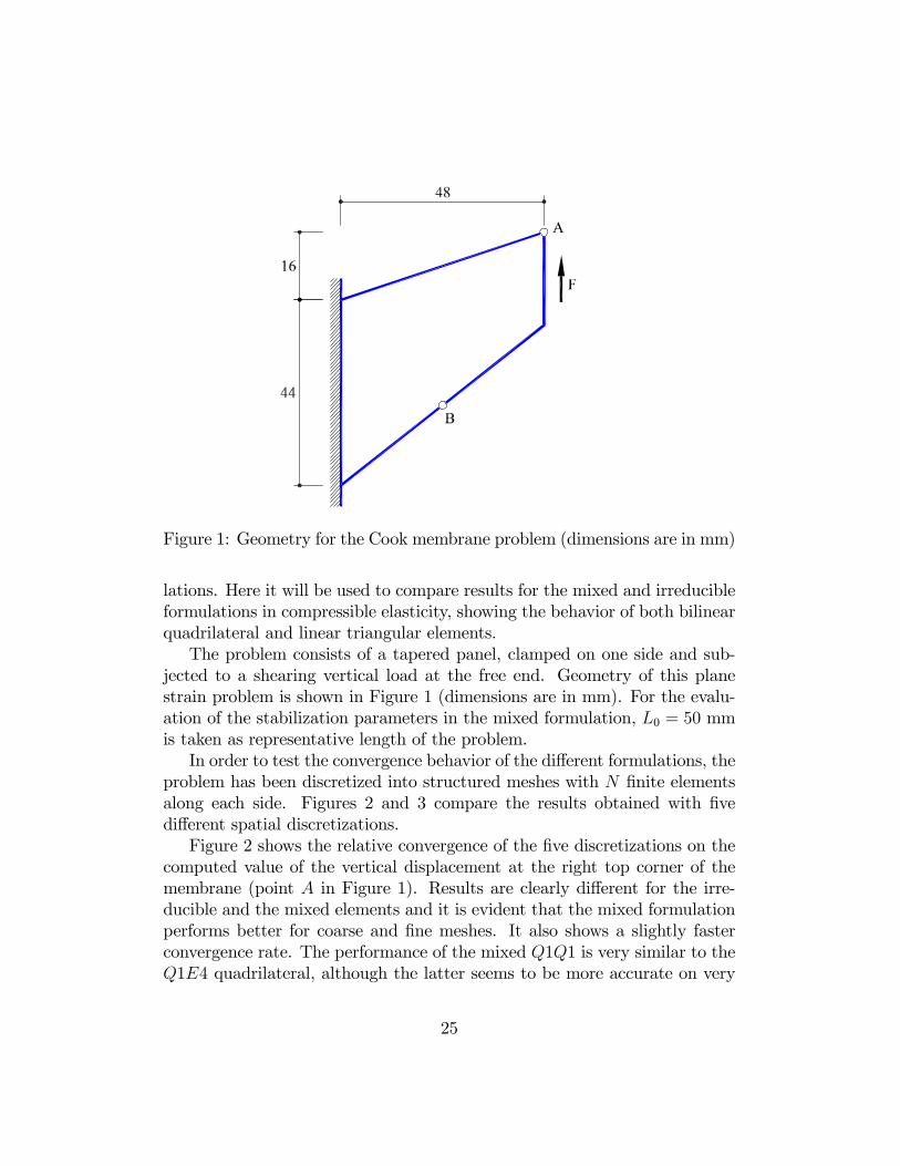
Figure 1: Geometry for the Cook membrane problem (dimensions are in mm)
lations. Here it will be used to compare results for the mixed and irreducibleformulations in compressible elasticity, showing the behavior of both bilinearquadrilateral and linear triangular elements.The problem consists of a tapered panel, clamped on one side and sub-
jected to a shearing vertical load at the free end. Geometry of this planestrain problem is shown in Figure 1 (dimensions are in mm). For the evalu-ation of the stabilization parameters in the mixed formulation, L0 = 50 mmis taken as representative length of the problem.In order to test the convergence behavior of the di¤erent formulations, the
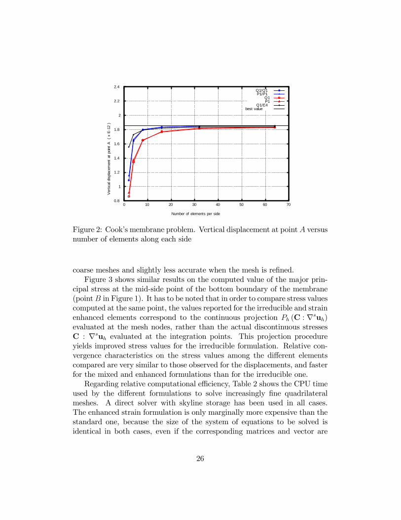
problem has been discretized into structured meshes with N �nite elementsalong each side. Figures 2 and 3 compare the results obtained with �vedi¤erent spatial discretizations.Figure 2 shows the relative convergence of the �ve discretizations on the
computed value of the vertical displacement at the right top corner of themembrane (point A in Figure 1). Results are clearly di¤erent for the irre-ducible and the mixed elements and it is evident that the mixed formulationperforms better for coarse and �ne meshes. It also shows a slightly fasterconvergence rate. The performance of the mixed Q1Q1 is very similar to theQ1E4 quadrilateral, although the latter seems to be more accurate on very
25
0.8
1
1.2
1.4
1.6
1.8
2
2.2
2.4
0 10 20 30 40 50 60 70
Ver
tical
dis
plac
emen
t at
poi
nt A
(
x E
12
)
Number of elements per side
Q1/Q1P1/P1
Q1P1
Q1/E4best value
Figure 2: Cook�s membrane problem. Vertical displacement at pointA versusnumber of elements along each side
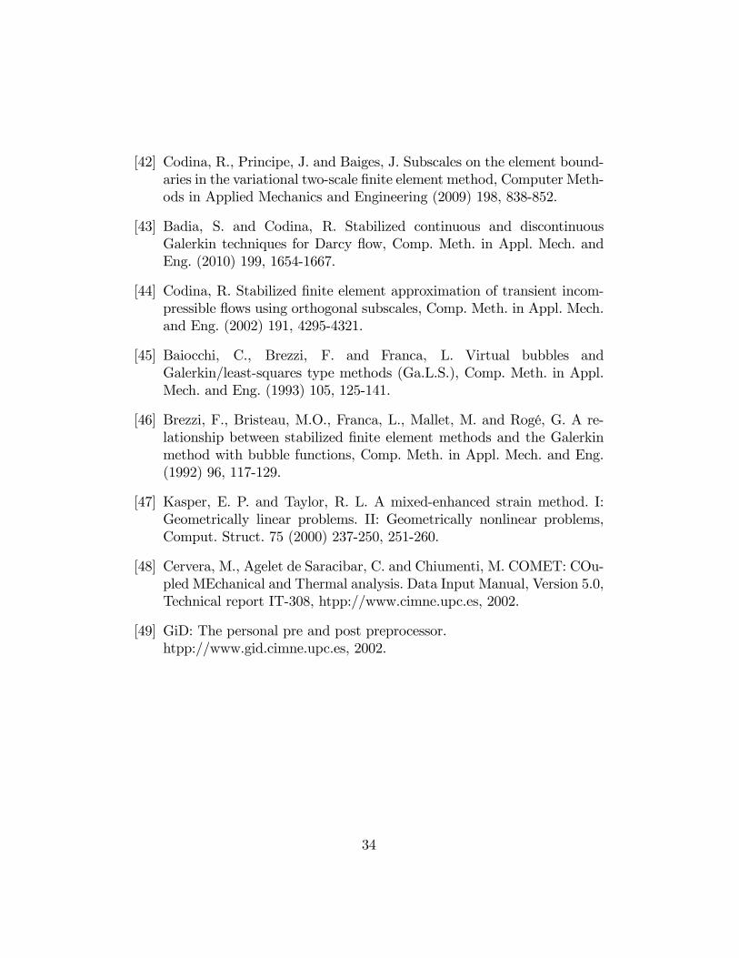
coarse meshes and slightly less accurate when the mesh is re�ned.Figure 3 shows similar results on the computed value of the major prin-
cipal stress at the mid-side point of the bottom boundary of the membrane(pointB in Figure 1). It has to be noted that in order to compare stress valuescomputed at the same point, the values reported for the irreducible and strainenhanced elements correspond to the continuous projection Ph (C : rsuh)evaluated at the mesh nodes, rather than the actual discontinuous stressesC : rsuh evaluated at the integration points. This projection procedureyields improved stress values for the irreducible formulation. Relative con-vergence characteristics on the stress values among the di¤erent elementscompared are very similar to those observed for the displacements, and fasterfor the mixed and enhanced formulations than for the irreducible one.Regarding relative computational e¢ ciency, Table 2 shows the CPU time
used by the di¤erent formulations to solve increasingly �ne quadrilateralmeshes. A direct solver with skyline storage has been used in all cases.The enhanced strain formulation is only marginally more expensive than thestandard one, because the size of the system of equations to be solved isidentical in both cases, even if the corresponding matrices and vector are
26
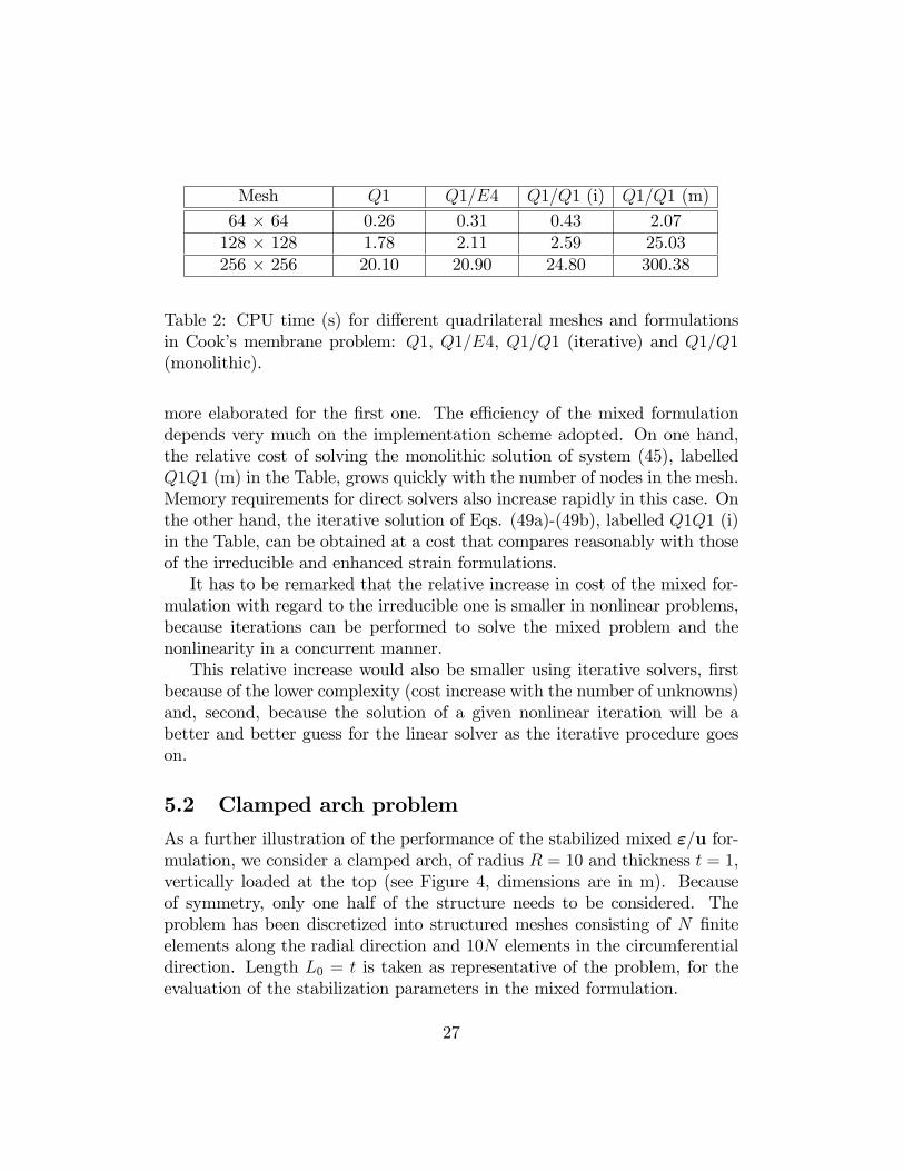
Mesh Q1 Q1=E4 Q1=Q1 (i) Q1=Q1 (m)64 � 64 0.26 0.31 0.43 2.07128 � 128 1.78 2.11 2.59 25.03256 � 256 20.10 20.90 24.80 300.38
Table 2: CPU time (s) for di¤erent quadrilateral meshes and formulationsin Cook�s membrane problem: Q1, Q1=E4, Q1=Q1 (iterative) and Q1=Q1(monolithic).
more elaborated for the �rst one. The e¢ ciency of the mixed formulationdepends very much on the implementation scheme adopted. On one hand,the relative cost of solving the monolithic solution of system (45), labelledQ1Q1 (m) in the Table, grows quickly with the number of nodes in the mesh.Memory requirements for direct solvers also increase rapidly in this case. Onthe other hand, the iterative solution of Eqs. (49a)-(49b), labelled Q1Q1 (i)in the Table, can be obtained at a cost that compares reasonably with thoseof the irreducible and enhanced strain formulations.It has to be remarked that the relative increase in cost of the mixed for-
mulation with regard to the irreducible one is smaller in nonlinear problems,because iterations can be performed to solve the mixed problem and thenonlinearity in a concurrent manner.This relative increase would also be smaller using iterative solvers, �rst
because of the lower complexity (cost increase with the number of unknowns)and, second, because the solution of a given nonlinear iteration will be abetter and better guess for the linear solver as the iterative procedure goeson.
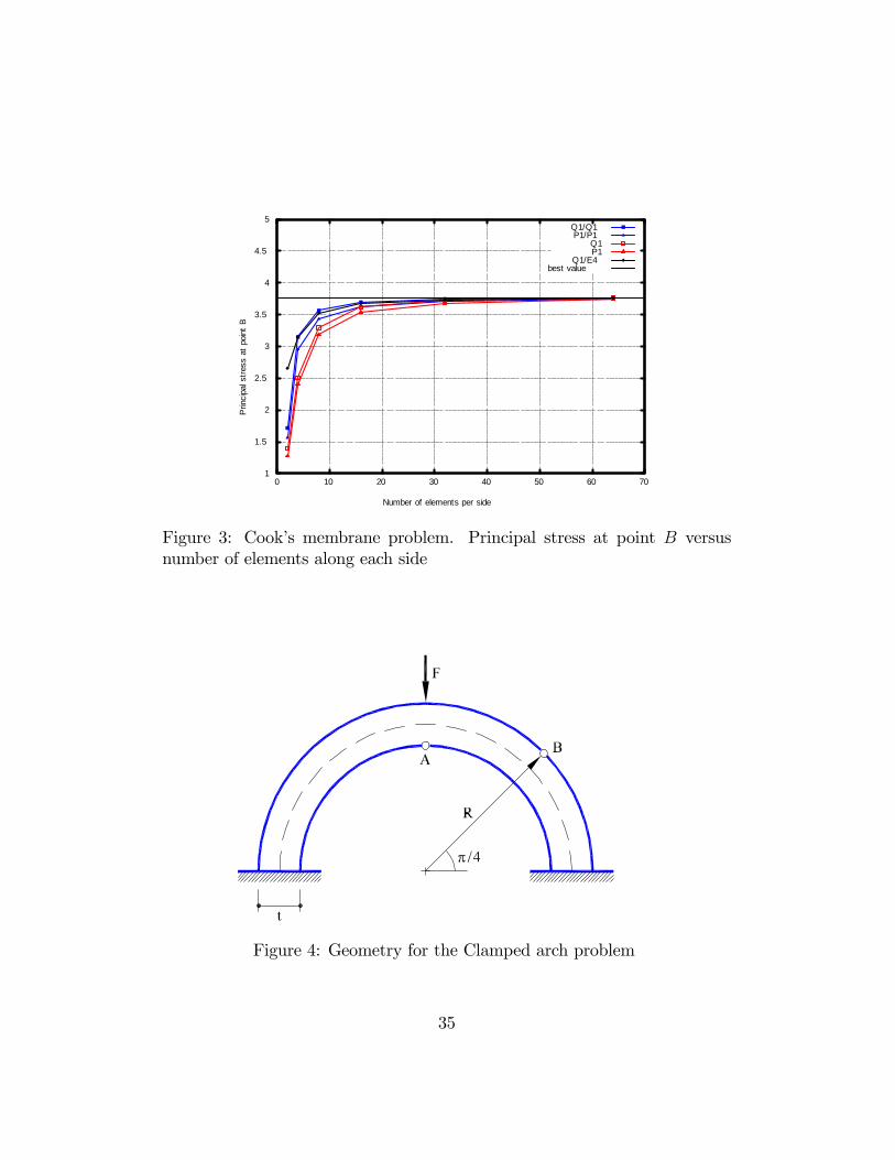
5.2 Clamped arch problem
As a further illustration of the performance of the stabilized mixed "=u for-mulation, we consider a clamped arch, of radius R = 10 and thickness t = 1,vertically loaded at the top (see Figure 4, dimensions are in m). Becauseof symmetry, only one half of the structure needs to be considered. Theproblem has been discretized into structured meshes consisting of N �niteelements along the radial direction and 10N elements in the circumferentialdirection. Length L0 = t is taken as representative of the problem, for theevaluation of the stabilization parameters in the mixed formulation.
27
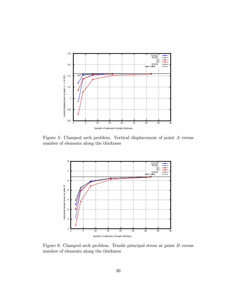
As in the previous example, Figures 5 and 6 compare the results ob-tained with �ve di¤erent spatial discretizations: Q1=Q1, P1=P1; Q1, Q1E4and P1. Figure 5 shows the relative convergence of the �ve discretizationsused on the computed value of the vertical displacement under the point load(point A in Figure 4). In this case, the mixed interpolations also show im-proved performance over their corresponding irreducible formulations in thedisplacement results. The quadrilateral mixed elements also compare wellwith the quadrilaterals with enhanced strains, which are very accurate forall meshes.Figure 6 shows results on the computed value of the major principal
stress at point B on the outer face of the arch (see Figure 4). The valuesreported for the irreducible and enhanced elements correspond to the con-tinuous projection Ph (C : rsuh) evaluated at the mesh nodes. Again, themixed formulations show better accuracy that the corresponding irreducibleones. The quadrilateral mixed elements and the quadrilateral elements withenhanced strains show almost identical performance in terms of stresses.
5.3 Sharp V-notched specimen under tension
For this last example, let us consider the vertical stretching of a square V-notched specimen as the one shown in Figure 7. Dimensions of the sampleare 2 � 2 m � m (width � height) and the V-shaped notch has a length of1 m and a maximum width at the boundary of 0.02 m. For the evaluationof the stabilization parameters in the mixed formulation, L0 = 1 m is takenas representative length of the problem. Uniform vertical displacements ofopposed sign are imposed at the top and bottom boundaries.In the continuous elastic problem associated to this situation, the strain
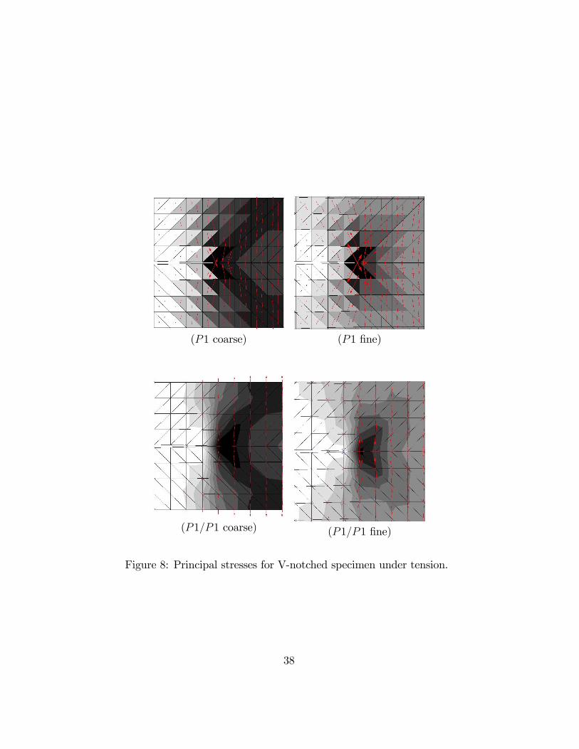
and stress �elds are singular at the tip of the sharp notch. The discretemodel corresponding to the irreducible �nite element formulation performssatisfactorily in terms of a global error norm, but approximates very poorlythe actual behavior near the singular points.To show this, a coarse structured mesh consisting of 8 � 8 � 2 P1 trian-
gles with a �45o bias is constructed. Figure 8(P1 coarse) depicts principalstresses computed on this mesh, plotted on top of the contour lines for themajor principal stress value. Note the strong mesh bias dependence that isobserved in front of and behind the notch tip. In fact, the largest values ofthe stresses occur behind the tip (left of the tip in the Figure), rather thanin front of it (right of the tip in the Figure). Computed stress directions near
28
the tip of the crack also show strong mesh bias dependence. Figure 8(P1 �ne)depicts principal stresses computed on a �ner structured mesh consisting of64 � 64 � 2 P1 triangles with the same �45o bias. A zoom on the areaaround the tip of the crack is shown, where the same errors as in the coarsemesh are displayed. Comparing the results obtained for both meshes, it canbe appreciated that the severe local errors caused by the mesh alignment arenot alleviated by mesh re�nement.Figures 8(P1=P1 coarse) and (P1=P1 �ne) show corresponding results
obtained used the stabilized mixed strain/displacement formulation on thesame coarse and �ne meshes. The improved accuracy with respect to theirreducible formulation is clear. In particular, the maximum principal stressvalue is detected exactly at the tip of the notch; computed stresses direc-tions are also noticeably improved. The importance of these two features innonlinear solid mechanics is evident. As it is shown in Part II of this work[40], they are crucial in strain localization problems where the constitutiveequation depends on the principal stress values and their directions.
6 Conclusions
This paper presents the formulation of stable mixed stress/displacement andstrain/displacement �nite elements using equal order interpolation for the so-lution of nonlinear problems is solid mechanics. The proposed stabilizationis based on the sub-grid scale approach and it circumvents the strictness ofthe compatibility conditions. The �nal method, consisting of stabilizing thestandard formulation for mixed elements with the projection of the displace-ment symmetric gradient, yields an accurate and robust scheme, suitable forengineering applications in 2D and 3D. Numerical examples show that resultscompare favorably with the corresponding irreducible formulations, showingimproved accuracy in the evaluation of the stress �eld. This characteristic isof great importance when facing nonlinear problems.
Acknowledgments
Financial support from the Spanish Ministry for Education and Science underthe SEDUREC project (CSD2006-00060) is acknowledged.
29
References
[1] Fraeijs de Veubeke, B.X. Displacement and equilibrium models in the�nite element method, in Stress Analysis, O.C. Zienkiewicz and G. Hol-lister, eds., Wiley (1965).
[2] Malkus, D.S. and Hughes, T.J.R. Mixed �nite element methods - re-duced and selective integration techniques: a uni�cation of concepts,Comp. Meth. in Appl. Mech. and Eng. (1978) 15, 63-81.
[3] Arnold, D.N., Brezzi, F. and Fortin, M. A stable �nite element for theStokes equations. Calcolo (1984) 21, 337-344.
[4] Simo, J.C., Taylor, R.L. and Pister, K.S. Variational and projectionmethods for the volume constraint in �nite deformation elasto-plasticity,Comp. Meth. in Appl. Mech. and Eng. (1985) 51, 177-208.
[5] Simo, J.C. and Rifai, M.S. A class of mixed assumed strain methodsand the method of incompatible modes, Int. Jour. for Num. Meths. inEng. (1990) 29, 1595-1638.
[6] Reddy, B.D. and Simo, J.C. Stability and convergence of a class of en-hanced assumed strain methods, SIAM J. Num. Anal. (1995) 32, 1705-1728.
[7] Bonet, J. and Burton, A.J. A simple average nodal pressure tetrahedralelement for incompressible and nearly incompressible dynamic explicitapplications. Comm. Num. Meths. in Eng. (1998)1 4, 437-449.
[8] Zienkiewicz, O.C., Rojek, J., Taylor, R.L. and Pastor, M. Triangles andtetrahedra in explicit dynamic codes for solids, Int. J. for Num. Meths.in Eng. (1998) 43, 565-583.
[9] Taylor, R.L. A mixed-enhanced formulation for tetrahedral elements,Int. Jour. for Num. Meths. in Eng. (2000) 47, 205-227.
[10] Dohrmann, C.R., Heinstein, M.W., Jung, J., Key, S.W. and Witkowsky,W.R. Node-based uniform strain elements for three-node triangular andfour-node tetrahedral meshes. Int. Jour. for Num. Meths. in Eng. (2000)47, 1549-1568.
30
[11] Bonet, J., Marriot, H. and Hassan, O. An averaged nodal deformationgradient linear tetrahedral element for large strain explicit dynamic ap-plications. Comm. Num. Meths. in Eng. (2001) 17, 551-561.
[12] Bonet, J., Marriot, H. and Hassan, O. Stability and comparison of dif-ferent linear tetrahedral formulations for nearly incompressible explicitdynamic applications. Int. Jour. for Num. Meths. in Eng. (2001) 50,119-133.
[13] Oñate, E., Rojek, J., Taylor, R.L. and Zienkiewicz, O.C. Linear tri-angles and tetrahedra for incompressible problem usung a �nite calcu-lus formulation, Proceedings of European Conference on ComputationalMechanics, ECCM, 2001.
[14] de Souza Neto, E.A., Pires, F.M.A. and Owen D.R.J. A new F-bar-method for linear triangles and tetrahedra in the �nite strain analysisof nearly incompressible solids, Proceedings of VII International Con-ference on Computational Plasticity, COMPLAS, 2003.
[15] Zienkiewicz, O.C. Taylor, R.L. Baynham, J.AW. Mixed and irreducibleformulations in �nite element analysis, in Hybrid and Mixed FiniteElement Methods, S.N. Atlury, R.H. Gallagher and O.C. Zienkiewicz,eds.,Wiley (1983).
[16] Zienkiewicz, O.C. and Taylor, R.L.. The Finite Element Method,Butterworth-Heinemann, Oxford, 2000.
[17] Bischo¤, M. and Bletzinger, K.-U. Improving stability and accuracy ofReissner-Mindlin plate �nite elements via algebraic subgrid scale stabi-lizatio,. Comp. Meth. in Appl. Mech. and Eng. (2004) 193, 1517-1528.
[18] Arnold, D.N. Mixed �nite element methods for elliptic problems. Com-put. Meth. Appl. Mech. Eng.(1990) 82, 281�300.
[19] Brezzi, F. and Fortin, M. Mixed and Hybrid Finite Element Methods,Spinger, New York, 1991.
[20] Brezzi, F., Fortin, M. and Marini, D. Mixed �nite element methods withcontinuous stresses, Math. Models Meth. Appl. Sci. (1993) 3 ,275-287.
31
[21] Mijuca, D. On hexahedral �nite element HC8/27 in elasticity, Compu-tational Mechanics (2004) 33, 466-480.
[22] D.N. Arnold and R. Winther. Mixed �nite elements for elasticity, Nu-merische Mathematik (2002) 92, 401-419.
[23] D.N. Arnold, G. Awanou, and R.Winther. Finite elements for symmetrictensors in three dimensions, Math. Comput. (2008) 77, 1229-1251.
[24] Hughes, T.J.R. Multiscale phenomena: Green0s function, Dirichlet-toNeumann formulation, subgrid scale models, bubbles and the origins ofstabilized formulations, Comp. Meth. in Appl. Mech. and Eng. (1995)127, 387-401.
[25] Hughes, T.J.R., Feijoó, G.R., Mazzei. L., Quincy, J.B. The variationalmultiscale method-a paradigm for computational mechanics, Comp.Meth. in Appl. Mech. and Eng. (1998) 166, 3-28.
[26] Codina, R. and Blasco, J. A �nite element method for the Stokes prob-lem allowing equal velocity-pressure interpolations, Comp. Meth. inAppl. Mech. and Eng. (1997) 143, 373-391.
[27] Codina, R. Stabilization of incompressibility and convection throughorthogonal sub-scales in �nite element methods, Comp. Meth. in Appl.Mech. and Eng. (2000) 190, 1579-1599.
[28] Codina, R. Analysis of a stabilized �nite element approximation of theOseen equations using orthogonal subscales, Applied Numerical Mathe-matics (2008) 58, 264-283.
[29] Codina, R. Finite element approximation of the three �eld formulationof the Stokes problem using arbitrary interpolations, SIAM Journal onNumerical Analysis (2009) 47, 699-718.
[30] Badia, S. and Codina, R. Uni�ed stabilized �nite element formulationsfor the Stokes and the Darcy problems, SIAM Journal on NumericalAnalysis (2009) 17, 309-330.
[31] Chiumenti, M., Valverde, Q., Agelet de Saracibar, C. and Cervera, M. Astabilized formulation for incompressible elasticity using linear displace-ment and pressure interpolations, Comp. Meth. in Appl. Mech. and Eng.(2002) 191, 5253-5264.
32
[32] Cervera, M., Chiumenti, M., Valverde, Q. and Agelet de Saracibar, C.Mixed Linear/linear Simplicial Elements for Incompressible Elasticityand Plasticity, Comp. Meth. in Appl. Mech. and Eng. (2003) 192, 5249-5263.
[33] Chiumenti, M., Valverde, Q., Agelet de Saracibar, C. and Cervera, M. Astabilized formulation for incompressible plasticity using linear trianglesand tetrahedra, Int. J. of Plasticity (2004) 20, 1487-1504.
[34] Cervera, M., Chiumenti, M. and Agelet de Saracibar, C. Softening, lo-calization and stabilization: capture of discontinuous solutions in J2plasticity, Int. J. for Num. and Anal. Meth. in Geomechanics (2004) 28,373-393.
[35] Cervera, M., Chiumenti, M. and Agelet de Saracibar, C. Shear bandlocalization via local J2 continuum damage mechanics, Comp. Meth. inAppl. Mech. and Eng. (2004) 193, 849-880.
[36] Cervera, M. and Chiumenti, M. Size e¤ect and localization in J2 plas-ticity, Int. J. of Solids and Structures (2009) 46, 3301-3312.
[37] Pastor, M., Li, T., Liu, X. and Zienkiewicz, O.C. Stabilized low-order�nite elements for failure and localization problems in undrained soilsand foundations, Comp. Meth. in Appl. Mech. and Eng. (1999), 174,219-234.
[38] Mabssout, M., Herreros, M.I. and Pastor, M. Wave propagation and lo-calization problems in saturated viscoplastic geomaterials, Comp. Meth.in Appl. Mech. and Eng. (2003), 192, 955-971.
[39] Mabssout, M. and Pastor, M. A Taylor-Galerkin algorithm for shockwave propagation and strain localization failure of viscoplastic continua,Int. Jour. for Num. Meths. in Eng. (2006) 68, 425-447.
[40] Cervera, M., Chiumenti, M. and Codina, R. Mixed stabilized �nite ele-ment methods in nonlinear solid mechanics. Part II: strain localization,Comp. Meth. in Appl. Mech. and Eng. (2010), in press.
[41] Djoko, J. K. , Lamichhane, B. P. , Reddy, B. D. and Wohlmuth, B. I.Conditions for equivalence between the Hu-Washizu and related formu-lations, and computational behavior in the incompressible limit. Comp.Meths. Appl. Mech. Engng 195 (2006) 4161-4178.
33
[42] Codina, R., Principe, J. and Baiges, J. Subscales on the element bound-aries in the variational two-scale �nite element method, Computer Meth-ods in Applied Mechanics and Engineering (2009) 198, 838-852.
[43] Badia, S. and Codina, R. Stabilized continuous and discontinuousGalerkin techniques for Darcy �ow, Comp. Meth. in Appl. Mech. andEng. (2010) 199, 1654-1667.
[44] Codina, R. Stabilized �nite element approximation of transient incom-pressible �ows using orthogonal subscales, Comp. Meth. in Appl. Mech.and Eng. (2002) 191, 4295-4321.
[45] Baiocchi, C., Brezzi, F. and Franca, L. Virtual bubbles andGalerkin/least-squares type methods (Ga.L.S.), Comp. Meth. in Appl.Mech. and Eng. (1993) 105, 125-141.
[46] Brezzi, F., Bristeau, M.O., Franca, L., Mallet, M. and Rogé, G. A re-lationship between stabilized �nite element methods and the Galerkinmethod with bubble functions, Comp. Meth. in Appl. Mech. and Eng.(1992) 96, 117-129.
[47] Kasper, E. P. and Taylor, R. L. A mixed-enhanced strain method. I:Geometrically linear problems. II: Geometrically nonlinear problems,Comput. Struct. 75 (2000) 237-250, 251-260.
[48] Cervera, M., Agelet de Saracibar, C. and Chiumenti, M. COMET: COu-pled MEchanical and Thermal analysis. Data Input Manual, Version 5.0,Technical report IT-308, htpp://www.cimne.upc.es, 2002.
[49] GiD: The personal pre and post preprocessor.htpp://www.gid.cimne.upc.es, 2002.
34
1
1.5
2
2.5
3
3.5
4
4.5
5
0 10 20 30 40 50 60 70
Prin
cipa
l str
ess
at p
oint
B
Number of elements per side
Q1/Q1P1/P1
Q1P1
Q1/E4best value
Figure 3: Cook�s membrane problem. Principal stress at point B versusnumber of elements along each side
Figure 4: Geometry for the Clamped arch problem
35
0.6
0.8
1
1.2
1.4
1.6
1.8
0 5 10 15 20 25 30 35 40
Ver
tical
dis
plac
emen
t at
poi
nt A
(
x E
09
)
Number of elements through thickness
Q1/Q1P1/P1
Q1P1
Q1/E4best value
Figure 5: Clamped arch problem. Vertical displacement of point A versusnumber of elements along the thickness
1
2
3
4
5
6
7
8
0 5 10 15 20 25 30 35 40
Hor
izon
tal t
ensi
le s
tres
s at
poi
nt B
Number of elements through thickness
Q1/Q1P1/P1
Q1P1
Q1/E4best value
Figure 6: Clamped arch problem. Tensile principal stress at point B versusnumber of elements along the thickness
36
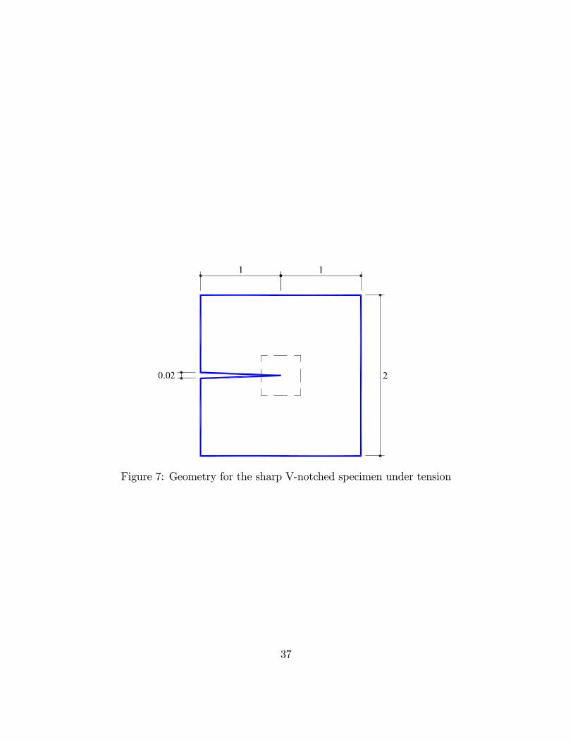
Figure 7: Geometry for the sharp V-notched specimen under tension
37
(P1 coarse) (P1 �ne)
(P1=P1 coarse) (P1=P1 �ne)
Figure 8: Principal stresses for V-notched specimen under tension.
38