Mixed-model analysis of agricultural experiments: …...Mixed-model analysis of agricultural...

Mixed-model analysis of agricultural experiments: when

some effects are random

Rong-Cai YangAlberta Agriculture and Rural Development

andUniversity of Alberta

[email protected]

CSA Statistics Symposium – GUELPH 09 August 7, 2009

mailto:[email protected]

Outline• Mixed‐model analysis

– Why mixed models?• Fixed vs. random effects

• GLM vs. MIXED

– Brief background theory– Three case studies

• RCBD experiment (when block effect is random)

• Unbalanced split‐plot experiment (estimability

problem)

• Long‐term experiment (modeling correlation between times)

Why MIXED analysis?• Most agricultural experiments have a mixture of fixed and

random effects – Treatments (e.g., types of fertilizers or herbicides) are fixed but

blocks, locations and years may be random.

• In the past, ANOVA or GLM procedures are used but they

are fixed‐effect models– GLM may give wrong denominator for F‐test– GLM may give wrong SE of a treatment– GLM assumes that all treatments have identical errors and such

errors are uncorrelated (IID assumption)

• SAS PROC MIXED is now available for correct analysis of data

sets – Allowing for a mixture of fixed and random effects – When IID assumption is not valid– No need for choosing SS1, SS2, SS3 or SS4 with unbalanced data

Uses of the MIXED analysis• Random effects (e.g., block effect in RBCD or split‐plot)

• Unbalanced data (estimability

problems)

• Repeated measures (long‐term experiments; growth

curve models)

• Spatial data (field experiments and precision farming)

• Heterogeneous variances

• Meta‐analysis (treat different study as a random effect)

• Non‐normal data PROC GLIMMIX

• Non‐linear data PROC NLMIXED

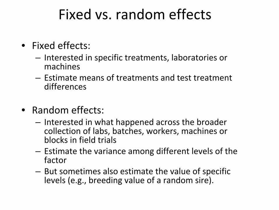
Fixed vs. random effects

• Fixed effects: – Interested in specific treatments, laboratories or

machines– Estimate means of treatments and test treatment

differences

• Random effects:– Interested in what happened across the broader

collection of labs, batches, workers, machines or

blocks in field trials– Estimate the variance among different levels of the

factor– But sometimes also estimate the value of specific

levels (e.g., breeding value of a random sire).

Pragmatic

approach to fixed vs. random effect debate

• There should be enough information in the data to estimate variance and covariance

parameters of random effects with sufficient precision.

• Some statisticians (e.g., Stroup and Mulitze 1991, Am. Stat. 45: 194‐200)

argue that a

factor should have more than 10 treatment levels

before it is considered

random.

MIXED = GLM + more• MIXED should be used…

but GLM remains

commonly used in the scientific literature for experiments with both fixed and random effects.

• Even if MIXED is used, GLM‐type interpretation is practiced

Why??– Many think GLM and MIXED give the same analysis– Stats textbooks provide little coverage on mixed models– Not familiar with MIXED syntax and outputs

Yang, R.-C. 2008. Why is MIXED analysis underutilized? Canadian Journal of Plant Science 88: 563-567.

Background theory

ANOVA model for multi-environment trials

Mixed model for multi-environment trials

Background TheoryProperties of mixed models

Under ANOVA model, G and R are simple

⎥⎥⎥

⎦

⎤

⎢⎢⎢

⎣

⎡

=

b

ge

e

I000I000I

G2

2

2

γ

τδ

δ

σσ

σand

But, G and R can be more complex under mixed models!!

Some common covariance structures for G

and R

BLUP of random effects• In some application of random‐effect models, the equivalent

of treatment means (fixed effects) may be of interest

• E.g., a random sample of sires may be used to estimate

variance components for genetic parameters but an animal

breeder may want to assess the genetic merit, known as the

“breeding value”

of each sire, conceptually similar to the

mean sire performance. However, because sire effects are

random and there is information about their probability

distribution, this affects how one estimates breeding value.

• Best linear unbiased prediction or BLUP is a mixed‐model

procedure to estimate a random effect by accounting for its

probability distribution:– BLUP of random effect = shrinkage factor*fixed effect

Some other BLUP applications• In clinical trials, random samples of patients provide

estimates of the mean performance of a treatment for the

population inference, but BLUPs

are essential for physicians

to monitor individual patients

• In quality control, a sample of workers can provide estimates

of the mean performance of a particular machine, but BLUPs

can help supervisors monitor the performance of individual

employees.

• In breeding or variety trials, a sample of environments can

provide estimates of the mean performance of a cultivar but

BLUPs

can help breeders or agronomists evaluate the

performance of individual environments.

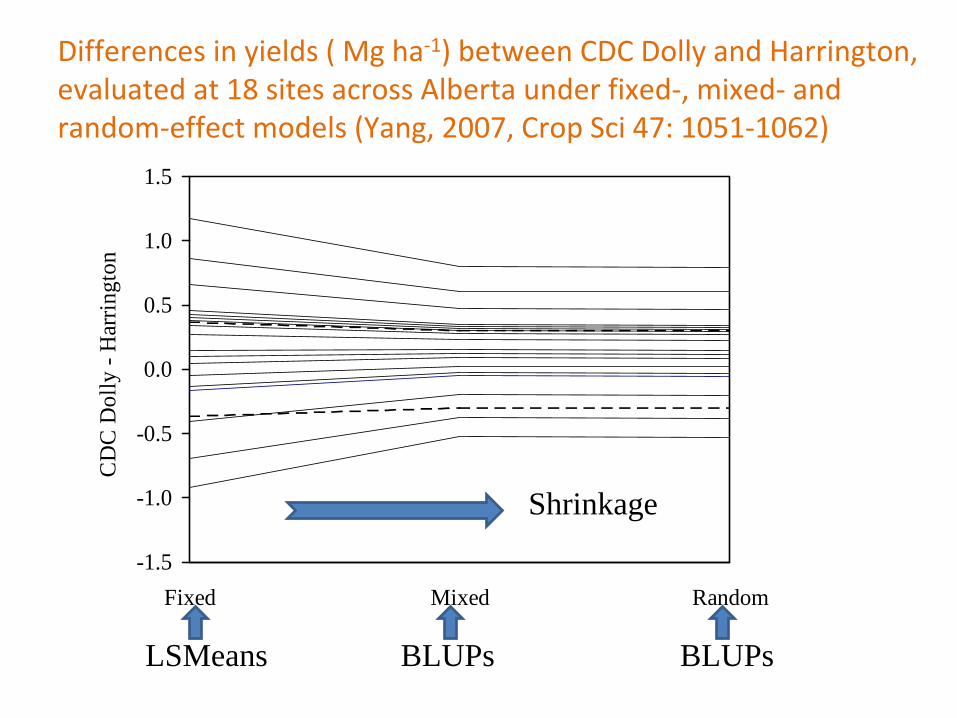
Differences in yields ( Mg ha‐1) between CDC Dolly and Harrington,

evaluated at 18 sites across Alberta under fixed‐, mixed‐

and

random‐effect models (Yang, 2007, Crop Sci

47: 1051‐1062)

-1.5

-1.0

-0.5

0.0

0.5

1.0

1.5

Fixed Mixed Random

CD

C D

olly

- H

arrin

gton

LSMeans BLUPs BLUPs

Shrinkage

ANOVA, ML or REML??• For balanced data, ANOVA = REML ≠

ML

– ML uses #obs

not df

to calculate residual variance and related

statistics

• For unbalanced

data, ML and REML are preferred over

any ANOVA method– ML or REML correctly calculates both rand and fixed effects but

ANOVA or GLM does not

• REML is often preferred over ML due to the fact ANOVA =

REML for balanced data– The default in SAS PROC MIXED is REML!

MIXED vs. GLM• MIXED is a generalization of GLM

• MIXED offers TYPE I ‐

III tests for fixed effects whereas

GLM offers TYPE I‐IV tests

• GLM has a MEANS and a LSMEANS statement where

MIXED only has a LSMEANS statement

• The RANDOM and REPEATED statements are used

differently

• GLM uses method‐of‐moments (or ANOVA) to estimate

the variance components; MIXED uses restricted/residual

maximum likelihood (REML), maximum likelihood (ML)

Case study #1: Mixed‐model analysis of RCBD experiment

(when block effect is random)

Data source: Littell

et al. 2002. SAS for linear Models, 4th

ed. P. 62‐71.

An example for PROC MIXED analysis of RCBD with random blocks

/*Five methods of applying irrigation are applied to a Valencia orange free grove. The tree in the grove are arranged in RCBD with eight blocks to account for local variation. At harvest, for each plot the fruit is weighed in pounds */

data methods;input irrig $ @@;do bloc=1 to 8;input fruitwt @@;logfwt=log(fruitwt);output;

end;datalines;trickle 450 469 249 125 280 352 221 251basin 358 512 281 58 352 293 283 186spray 331 402 183 70 258 281 219 46sprnkler 317 423 379 63 289 239 269 357flood 245 380 263 62 336 282 171 98;

proc glm data=methods;class bloc irrig;model fruitwt=bloc irrig;

proc mixed data=methods;class bloc irrig;model fruitwt=irrig;random bloc;

VS.

Random‐blocks ANOVA using PROC MIXED

Covariance ParameterEstimates

Cov Parm Estimate

bloc 10793 = var(block)Residual 3362.38 = var(error)

Fit Statistics

-2 Res Log Likelihood 413.8AIC (smaller is better) 417.8AICC (smaller is better) 418.2BIC (smaller is better) 417.9

Type 3 Tests of Fixed Effects

Num DenEffect DF DF F Value Pr > F

irrig 4 28 3.27 0.0254

Same as obtained from GLM analysis

LSMeans

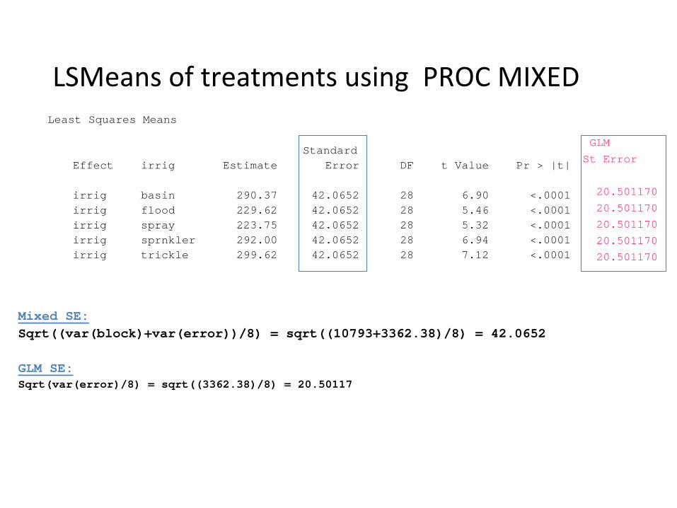
of treatments using PROC MIXEDLeast Squares Means

StandardEffect irrig Estimate Error DF t Value Pr > |t|

irrig basin 290.37 42.0652 28 6.90 <.0001irrig flood 229.62 42.0652 28 5.46 <.0001irrig spray 223.75 42.0652 28 5.32 <.0001irrig sprnkler 292.00 42.0652 28 6.94 <.0001irrig trickle 299.62 42.0652 28 7.12 <.0001

Mixed SE:Sqrt((var(block)+var(error))/8) = sqrt((10793+3362.38)/8) = 42.0652

GLM SE:Sqrt(var(error)/8) = sqrt((3362.38)/8) = 20.50117

GLM

St Error

20.501170

20.50117020.501170

20.50117020.501170

Pairwise

Treatment differences (LSD) using PROC MIXED

Differences of Least Squares Means

StandardEffect irrig _irrig Estimate Error DF t Value Pr > |t|

irrig basin flood 60.7500 28.9930 28 2.10 0.0453irrig basin spray 66.6250 28.9930 28 2.30 0.0292irrig basin sprnkler -1.6250 28.9930 28 -0.06 0.9557irrig basin trickle -9.2500 28.9930 28 -0.32 0.7521irrig flood spray 5.8750 28.9930 28 0.20 0.8409irrig flood sprnkler -62.3750 28.9930 28 -2.15 0.0402irrig flood trickle -70.0000 28.9930 28 -2.41 0.0225irrig spray sprnkler -68.2500 28.9930 28 -2.35 0.0258irrig spray trickle -75.8750 28.9930 28 -2.62 0.0141irrig sprnkler trickle -7.6250 28.9930 28 -0.26 0.7945

The SE of a treatment difference is not affected by the block effect (i.e., it doesn’t matter if blocks are random or fixed)....so GLM and MIXED SE are the same:

Sqrt(2*var(error)/8) = sqrt(2*3362.38/8) = 28.993

Mixed model for RCBD with random blocks

• Inference for treatment differences

is identical for fixed blocks (PROC GLM) and random blocks (PROC MIXED)

• However, if the focus is on estimating treatment means, then the choice of fixed‐

vs. random‐

blocks matters greatly.– Question: given the results of this study, how does

one anticipate the mean fruit weight of a irrigation

method in a different orchard??

Case study #2: Mixed‐model analysis of split‐plot

experiments: balanced and unbalanced

Data source: Littell et al. 1996. SAS system for mixed

models (p.58-75)

Data for split‐plot experiment

/*A split-plot experiment is carried out to examine the effect on dry weight yields (drywt) of 3 bacterial inoculi applied to two cultivars of grasses (A and B). The experiment has four blocks (rep) with cultivar (cult) as a main plot factor and inoculi (inoc) as the subplot factor.*/

Obs rep cult inoc drywt

1 1 a con 27.42 1 a dea 29.73 1 a liv 34.54 1 b con 29.45 1 b dea 32.56 1 b liv 34.47 2 a con 28.98 2 a dea 28.79 2 a liv 33.4

10 2 b con 28.711 2 b dea 32.412 2 b liv 36.413 3 a con 28.614 3 a dea 29.715 3 a liv 32.916 3 b con 27.217 3 b dea 29.118 3 b liv 32.619 4 a con 26.720 4 a dea 28.921 4 a liv 31.822 4 b con 26.823 4 b dea 28.624 4 b liv 30.7

PROC GLM for split‐plot experiment

proc glm;class rep cult inoc;model drywt = rep cult rep*cult inoc cult*inoc/ss3;

test h=cult e=rep*cult;random rep cult*rep/test;

run;

PROC GLM for split-plot experiment

proc glm;class rep cult inoc;model drywt = rep cult rep*cult inoc cult*inoc;

test h=cult e=rep*cult;random rep cult*rep/test;run;

Two sizes of experiment units, main-plots and subplots…so need two error terms, one for the main-plots called error a (= rep*cult) and the other for the subplots called error b

Source dfReplication 3Cultivar 1Error a (rep x cult) 3inoculi 2cultivar x inoculi 2Error b 12

Two diff ways to ensure correct testing for cultivar effect

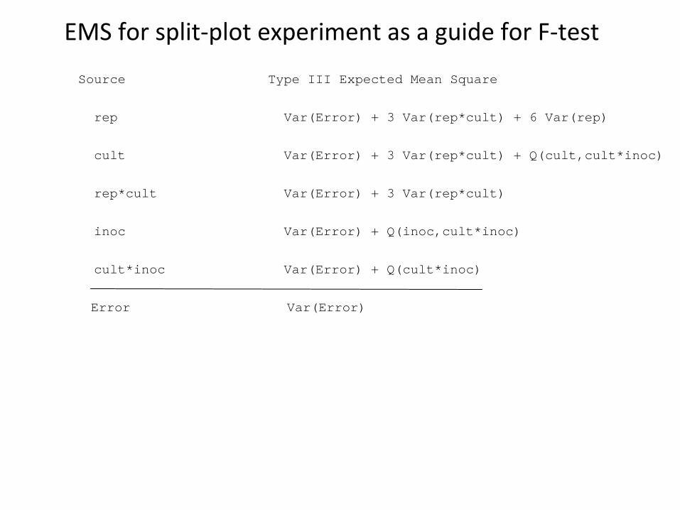
EMS for split‐plot experiment as a guide for F‐test

Source Type III Expected Mean Square

rep Var(Error) + 3 Var(rep*cult) + 6 Var(rep)

cult Var(Error) + 3 Var(rep*cult) + Q(cult,cult*inoc)

rep*cult Var(Error) + 3 Var(rep*cult)

inoc Var(Error) + Q(inoc,cult*inoc)

cult*inoc Var(Error) + Q(cult*inoc)

Error Var(Error)

GLM output for split‐plot experiment:

Using TEST statement

Source DF Squares Mean Square F Value Pr > F

Model 11 157.2083333 14.2916667 20.26 <.0001

Error 12 8.4650000 0.7054167

Corrected Total 23 165.6733333

Source DF Type III SS Mean Square F Value Pr > F

rep 3 25.3200000 8.4400000 11.96 0.0006cult 1 2.4066667 2.4066667 3.41 0.0895rep*cult 3 9.4800000 3.1600000 4.48 0.0249inoc 2 118.1758333 59.0879167 83.76 <.0001cult*inoc 2 1.8258333 0.9129167 1.29 0.3098

Tests of Hypotheses Using the Type III MS for rep*cult as an Error Term


cult 1 2.40666667 2.40666667 0.76 0.4471

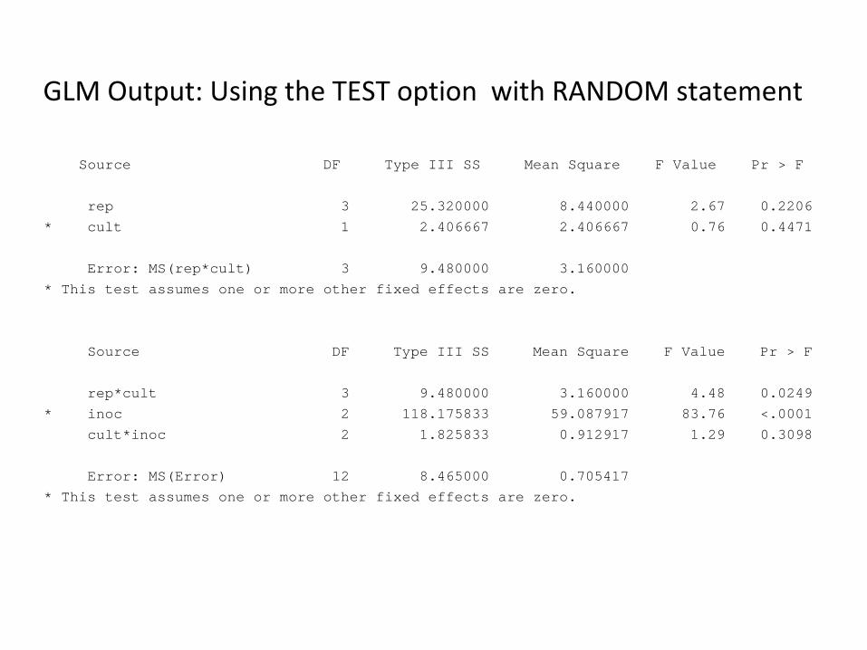
GLM Output: Using the TEST option with RANDOM statement


rep 3 25.320000 8.440000 2.67 0.2206* cult 1 2.406667 2.406667 0.76 0.4471

Error: MS(rep*cult) 3 9.480000 3.160000* This test assumes one or more other fixed effects are zero.


rep*cult 3 9.480000 3.160000 4.48 0.0249* inoc 2 118.175833 59.087917 83.76 <.0001

cult*inoc 2 1.825833 0.912917 1.29 0.3098

Error: MS(Error) 12 8.465000 0.705417* This test assumes one or more other fixed effects are zero.

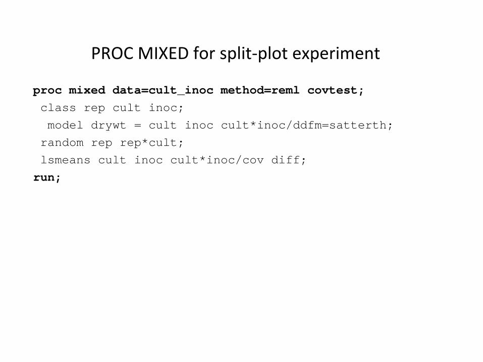
PROC MIXED for split‐plot experiment

proc mixed data=cult_inoc method=reml covtest;class rep cult inoc;

model drywt = cult inoc cult*inoc/ddfm=satterth;random rep rep*cult;lsmeans cult inoc cult*inoc/cov diff;

run;

PROC MIXED analysis for split‐plot experiment

Test for variances of random effects

Standard ZCov Parm Estimate Error Value Pr > Z

rep 0.8800 1.2264 0.72 0.2365rep*cult 0.8182 0.8654 0.95 0.1722Residual 0.7054 0.2880 2.45 0.0072

Test for fixed effects



cult 1 3 0.76 0.4471inoc 2 12 83.76 <.0001cult*inoc 2 12 1.29 0.3098

Determining SE for mean comparisons in split‐plot experiment:

GLM vs. MIXEDproc glm data=cult_inoc;class rep cult inoc;model drywt = rep cult rep*cult inoc cult*inoc;estimate 'Cult a vs cult b' cult 1 -1;estimate 'con vs dea' inoc 1 -1;estimate 'con vs dea in cult a' inoc 1 -1 0 cult*inoc 1 -1 0 0 0 0;estimate 'Cult a vs cult b in con' cult 1 -1 cult*inoc 1 0 0 -1 0 0;

run;

proc mixed data=cult_inoc method=reml;class rep cult inoc;model drywt = cult inoc cult*inoc/ddfm=satterth;random rep cult*rep;

*The following 4 ESTIMATE statements give correct SE for comparisons;estimate 'Cult a vs cult b' cult 1 -1;estimate 'con vs dea' inoc 1 -1;estimate 'con vs dea in cult a' inoc 1 -1 0 cult*inoc 1 -1 0 0 0 0;estimate 'Cult a vs cult b in con' cult 1 -1 cult*inoc 1 0 0 -1 0 0;

run;

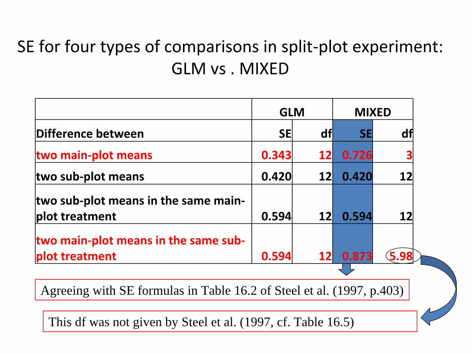
SE for four types of comparisons in split‐plot experiment: GLM vs

. MIXED

GLM MIXED

Difference between SE df SE df

two main‐plot means 0.343 12 0.726 3

two sub‐plot means 0.420 12 0.420 12

two sub‐plot means in the same main‐

plot treatment 0.594 12 0.594 12

two main‐plot means in the same sub‐

plot treatment 0.594 12 0.873 5.98

Agreeing with SE formulas in Table 16.2 of Steel et al. (1997, p.403)

This df was not given by Steel et al. (1997, cf. Table 16.5)

Unbalanced split‐plot experiment /*The same split-plot experiment as given in Littell et al. 1996. SAS

system for mixed models (p.58-75), but assuming that all of the observations for rep 1, cult ‘a’ were lost*/

Obs rep cult inoc drywt

1 1 a con .2 1 a dea .3 1 a liv .4 1 b con 29.45 1 b dea 32.56 1 b liv 34.47 2 a con 28.98 2 a dea 28.79 2 a liv 33.4

10 2 b con 28.711 2 b dea 32.412 2 b liv 36.413 3 a con 28.614 3 a dea 29.715 3 a liv 32.916 3 b con 27.217 3 b dea 29.118 3 b liv 32.619 4 a con 26.720 4 a dea 28.921 4 a liv 31.822 4 b con 26.823 4 b dea 28.624 4 b liv 30.7

Missing values

GLM analysis

proc glm;class rep cult inoc;model drywt2 = rep cult rep*cult inoc cult*inoc;test h=cult e=rep*cult;random rep cult*rep/test;lsmeans cult/stderr tdiff e=rep*cult;lsmeans inoc /stderr tdiff;lsmeans cult*inoc/stderr tdiff;run;

Problem I with GLM analysis

Source DF Type I SS Mean Square F Value Pr > F




Type I and III SS for some effects are different due to imbalance

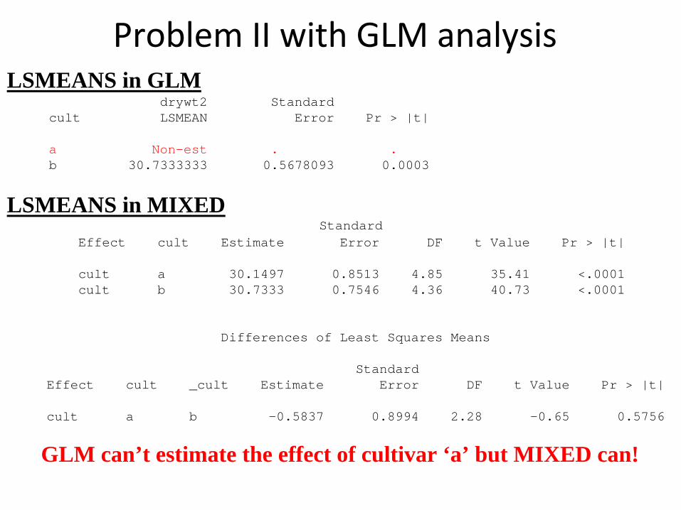
Problem II with GLM analysis

drywt2 Standardcult LSMEAN Error Pr > |t|

a Non-est . .b 30.7333333 0.5678093 0.0003

GLM can’t estimate the effect of cultivar ‘a’ but MIXED can!

StandardEffect cult Estimate Error DF t Value Pr > |t|

cult a 30.1497 0.8513 4.85 35.41 <.0001cult b 30.7333 0.7546 4.36 40.73 <.0001

Differences of Least Squares Means

StandardEffect cult _cult Estimate Error DF t Value Pr > |t|

cult a b -0.5837 0.8994 2.28 -0.65 0.5756

LSMEANS in GLM

LSMEANS in MIXED

Why GLM has estimability

problems?

• GLM tries to find an estimable linear combination over all fixed and random

effects, as if they were all fixed.

• Since there is a missing block*cult cell, no estimable combination can be found.

• GLM falsely declares LSMeans

for cult ‘a’

to be non‐estimable when they are actually all estimable with MIXED.

Case study #3: Mixed‐model analysis of long‐term

experiment

Data source: Petersen. 1994. Agricultural Field Experiments: Design and analysis (Table 7.7)

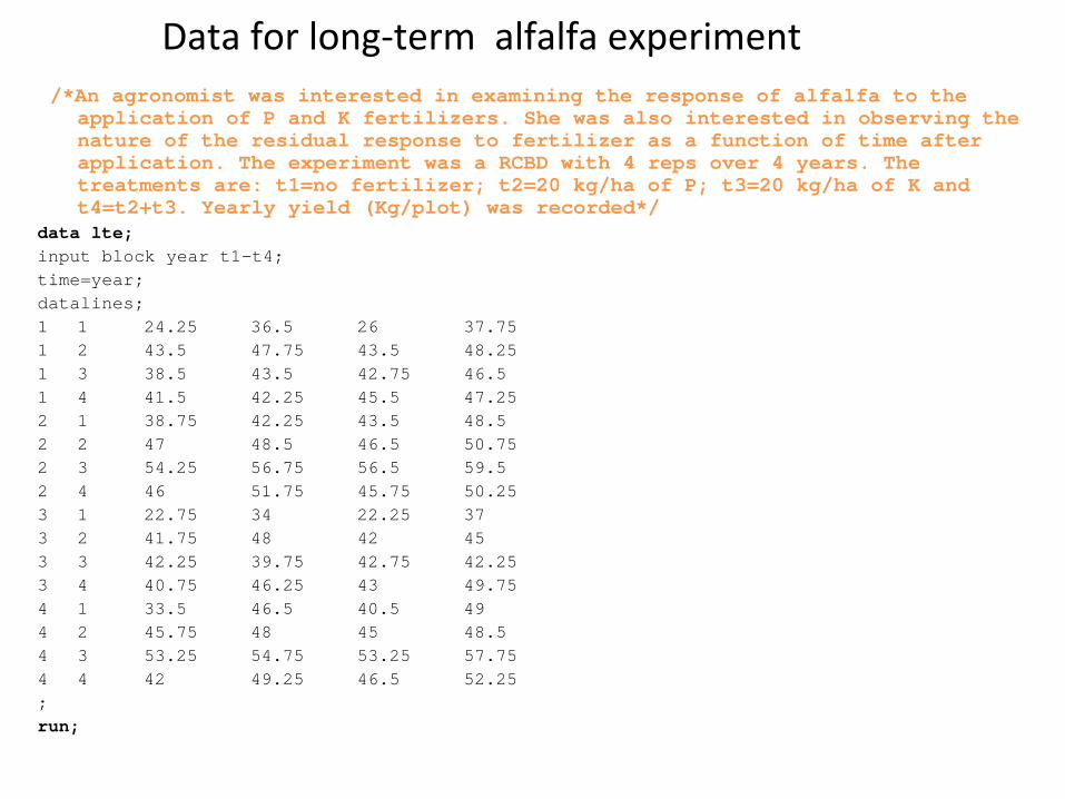
Data for long‐term alfalfa experiment/*An agronomist was interested in examining the response of alfalfa to the

application of P and K fertilizers. She was also interested in observing the nature of the residual response to fertilizer as a function of time after application. The experiment was a RCBD with 4 reps over 4 years. The treatments are: t1=no fertilizer; t2=20 kg/ha of P; t3=20 kg/ha of K and t4=t2+t3. Yearly yield (Kg/plot) was recorded*/

data lte;input block year t1-t4;time=year;datalines;1 1 24.25 36.5 26 37.751 2 43.5 47.75 43.5 48.251 3 38.5 43.5 42.75 46.51 4 41.5 42.25 45.5 47.252 1 38.75 42.25 43.5 48.52 2 47 48.5 46.5 50.752 3 54.25 56.75 56.5 59.52 4 46 51.75 45.75 50.253 1 22.75 34 22.25 373 2 41.75 48 42 453 3 42.25 39.75 42.75 42.253 4 40.75 46.25 43 49.754 1 33.5 46.5 40.5 494 2 45.75 48 45 48.54 3 53.25 54.75 53.25 57.754 4 42 49.25 46.5 52.25;run;

W. G. Cochran. 1939. Long-Term Agricultural Experiments. Supplement to the Journal of the Royal Statistical Society 6:104-148

Analysis of a long-term experiment as a repeated measure experiment [Crop Sci. 46 (2006):2492-2502]

Different analyses of repeated measure experiments

• Summary statistics approach

• Split‐plot in time (Cochran 1939)

• Multivariate analysis of variance (MANOVA) – GLM with REPEATED

statement

• Direct modeling of correlation structure of times – MIXED analysis

Cochran’s (1939) model: Split‐plot in time

proc mixed data=lte2 method=type3 or reml;class block trt year;model yield=trt year trt*year;random block block*trt;run;

Trt are main plots and year (time) are subplots

Split‐plot in time: SAS output

Type 3 Analysis of Variance

Sum ofSource DF Squares Mean Square Expected Mean Square

block 3 1057.242187 352.414062 Var(Residual) + 4 Var(block*trt)+ 16 Var(block)

trt 3 489.781250 163.260417 Var(Residual) + 4 Var(block*trt)+ Q(trt,trt*year)

block*trt 9 17.304687 1.922743 Var(Residual) + 4 Var(block*trt)year 3 1463.429687 487.809896 Var(Residual) + Q(year,trt*year)trt*year 9 164.992188 18.332465 Var(Residual) + Q(trt*year)Residual 36 547.984375 15.221788 Var(Residual)

Problem with this data: negative estimate of variance for block*trt

Covariance Parameter Estimates

Cov Parm GLM Estimate REML Estimate

block 21.9057 21.2405block*trt -3.3248 0Residual 15.2218 12.5420

Affecting F-tests for fixed effects

Impact of negative estimate of variance component for block*trt

on F‐tests for

fixed effects


Num Den GLMEffect DF DF F Value Pr > F

trt 3 9 84.91 <.0001year 3 36 32.05 <.0001trt*year 9 36 1.20 0.3225

MIXEDF Value Pr > F

13.00 0.001338.83 <.00011.46 0.2005

Modeling correlation between times

Modeling correlation of times with MIXED analysis

proc mixed data=lte2 method=reml covtest scoring;class block trt year;model yield=trt year trt*year/ddfm=kr;random block(trt*year) block*trt(year); repeated year/subject=block*trt type=un r rcorr;lsmeans trt*year/diff slice=year;ods listing exclude lsmeans;ods listing exclude diffs;ods output diffs=un_diffs;run;

Covariance structures used in the TYPE= option for R

matrix

Why different covariance structures?• UN: the most complex cov

structure where each pair of times

has its own unique correlation• CS: the simplest correlation model (one corr

for all times)

• VC: no correlation between times (IID assumption is met)In the repeated measures, correlation between observations is

often a function of their distance in time: adjacent observations

tend to be more highly correlated than observations farther

apart.• AR(1): correlation between adjacent observations is ρ

but

correlation between observations d unit apart is ρd

(ρd <ρ). • TOEP is similar to AR(1) but there is no known function relating

ρd

to ρ.• ANTE(1) is a more general model that preserves the main

feature of AR(1) and TOEP but allows for unequal spacing or

appreciable change over time.

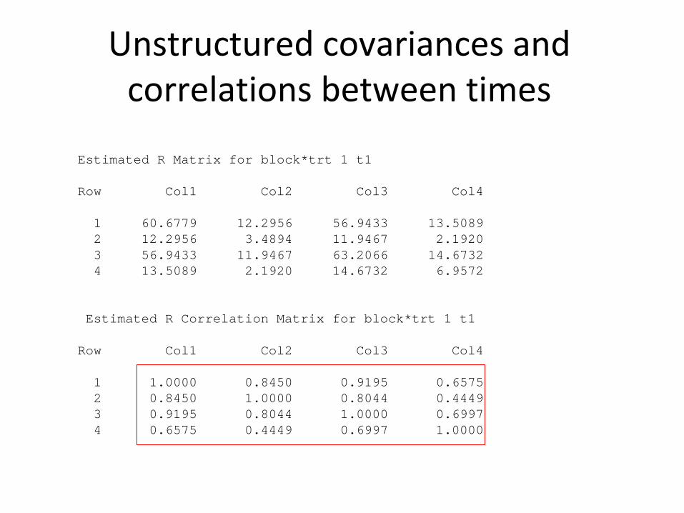
Unstructured covariances

and correlations between times

Estimated R Matrix for block*trt 1 t1

Row Col1 Col2 Col3 Col4

1 60.6779 12.2956 56.9433 13.50892 12.2956 3.4894 11.9467 2.19203 56.9433 11.9467 63.2066 14.67324 13.5089 2.1920 14.6732 6.9572

Estimated R Correlation Matrix for block*trt 1 t1

Row Col1 Col2 Col3 Col4

1 1.0000 0.8450 0.9195 0.65752 0.8450 1.0000 0.8044 0.44493 0.9195 0.8044 1.0000 0.69974 0.6575 0.4449 0.6997 1.0000

Fit statistics output from MIXED analysis

REML likelihood-2RLL = minus 2 times the maximum value of the restricted log likelihood and is used to compare models with same fixed effects but different covariance structures

Penalized REML likelihoodAIC =-2RLL+ 2dAICC = -2RLL+ 2d n/(n-d-1) BIC = -2RLL+ d logn

Fit Statistics

-2 Res Log Likelihood 253.0AIC (smaller is better) 275.0AICC (smaller is better) 282.3BIC (smaller is better) 268.2

Summary of fit statistics for different covariance structures

Cov

Structure ‐2RLL AIC BIC

VC (simple) 327.4 331.4 330.2

CS 310.4 316.4 314.5

AR(1) 310.6 316.6 314.7

TOEP 290.2 302.2 298.5

ANTE(1) 254.1 270.1 265.2

UN 253.0 277.0 269.6

So ANTE(1) is the best model as it has the smallest AIC and BIC!

F‐tests for fixed effects under different covariance structures

Cov

Structure Trt Year Trt*year

VC (simple) 4.83 (.0051) 14.43 (<.0001) 0.54 (.8362)

CS 1.82 (.1966) 32.05 (<.0001) 1.20 (.3225)

AR(1) 1.86 (.1879) 31.39 (<.0001) 1.19 (.3324)

TOEP 1.81 (.1983) 96.04 (<.0001) 3.69 (.0061)

ANTE(1) 1.82 (.1965) 74.47 (<.0001) 3.26 (.017)

UN 1.82 (.1969) 71.82 (<.0001) 2.88 (.0417)

SE of comparisons under different covariance structures

Comparison Estimate ANTE(1) AR(1) CS TOEP UN VC

Y1 vs Y2 at trt 1 ‐14.69 3.141 2.766 2.759 3.205 3.165 4.111

Y1 vs Y3 at trt 1 ‐17.25 1.649 2.782 2.759 1.454 1.619 4.111

Y1 vs Y4 at trt 1 ‐12.75 3.220 2.798 2.759 3.292 3.205 4.111

trt1 vs trt2 at Y 1 ‐10.00 5.513 4.092 4.111 4.122 5.519 4.111

trt1 vs trt3 at Y 1 ‐3.25 5.513 4.092 4.111 4.122 5.519 4.111

trt1 vs trt4 at Y 1 ‐13.25 5.513 4.092 4.111 4.122 5.519 4.111

Yield of Alfalfa in P‐K Fertilizer Trial ‐RCBD with 4 reps over 4 years

25

30

35

40

45

50

55

1 2 3 4

Year

Yiel

d (k

g/pl

ot)

No fertilizer

20 kg/ha P

20 kg/ha K

20 kg P + 20 kg K

From R.G. Petersen (1994) “Agricultural Field Experiments: Design and Analysis"

The figure suggests a quadratic response of time to alfalfa yield and such responses are not

homogeneous among the treatments.

The following SAS code is for such an analysis:

proc mixed data=lte2 method=reml scoring covtest noprofile;class block trt year;model yield=trt time trt*time time time2 trt*time trt*time2

/htype=1 ddfm=kr;random block(trt*year) block*trt(year);repeated /subject=block*trt type=ante(1) r rcorr;parms 1.1178 0.03064 59.6311 2.5707 62.1665 6.0416

0.9900 0.9422 0.7547/noiter;run;



trt 3 22.2 15.46 <.0001time 1 17.2 115.01 <.0001time*trt 3 17.2 2.92 0.0636time2 1 21.8 170.77 <.0001time2*trt 3 21.8 8.39 0.0007

• There is a significant quadratic component to the regression

•The slopes for the linear regressions are the same across the treatments (insignificant time*trt) but those for the quadratic components are not (significant time2*trt).

Take‐home messages

• GLM analysis should no longer be used unless a strictly fixed‐effect model is appropriate

• The pseudo‐use of MIXED analysis (i.e., use of MIXED with GLM‐type interpretation) is like

putting “new wine in old bottles”

• The true and full use of MIXED analysis accommodates many complex situations in real

experiments (e.g., unbalanced data and long‐term experiments), thereby enhancing values of these

experiments.

Mixed-model analysis of agricultural experiments: …...Mixed-model analysis of agricultural...

Documents

Transcript of Mixed-model analysis of agricultural experiments: …...Mixed-model analysis of agricultural...