Mixed Integer Programming Models for Non-Separable Piecewise Linear Cost Functions

INFORMS Annual Meeting 2008 – Washington, DC

Mixed Integer Programming Models for

Non-Separable Piecewise Linear Cost

Functions

Juan Pablo Vielma Shabbir Ahmed George Nemhauser

H. Milton Stewart School of Industrial and Systems Engineering

Georgia Institute of Technology

/20

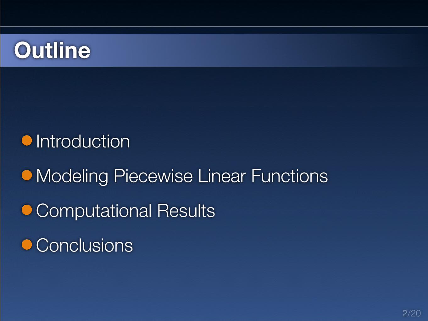
Outline

Introduction

Modeling Piecewise Linear Functions

Computational Results

Conclusions

2

is a piecewise linear function .

is any compact set. /20

Introduction

Piecewise Linear Optimization

3

/20

Introduction

Piecewise Linear Functions (PLF)

Approximate non-linearities,

discounts for volume, etc.

Many Applications.

Convex = Linear Programming.

Non-Convex = NP Hard.

Specialized algorithms (Tomlin

1981, ..., de Farias et al. 2008 ) or

Mixed Integer Programming Models

(12+ papers)

4

/20

Introduction

Non-Separable = Multivariate

Separable function:

Functions can sometimes be separated:

Undesirable for numerical reasons and strength.

Not possible for interpolated functions.5

/20


Modeling Function = Epigraph

Example: 6

0 1 2 4 5

f(4) = 50

f(0) = 10

f(1) = 32

f(2) = 40

f(5) = 15

(a) f .

0 1 2 4 5

50

10

32

40

15

(b) epi(f).

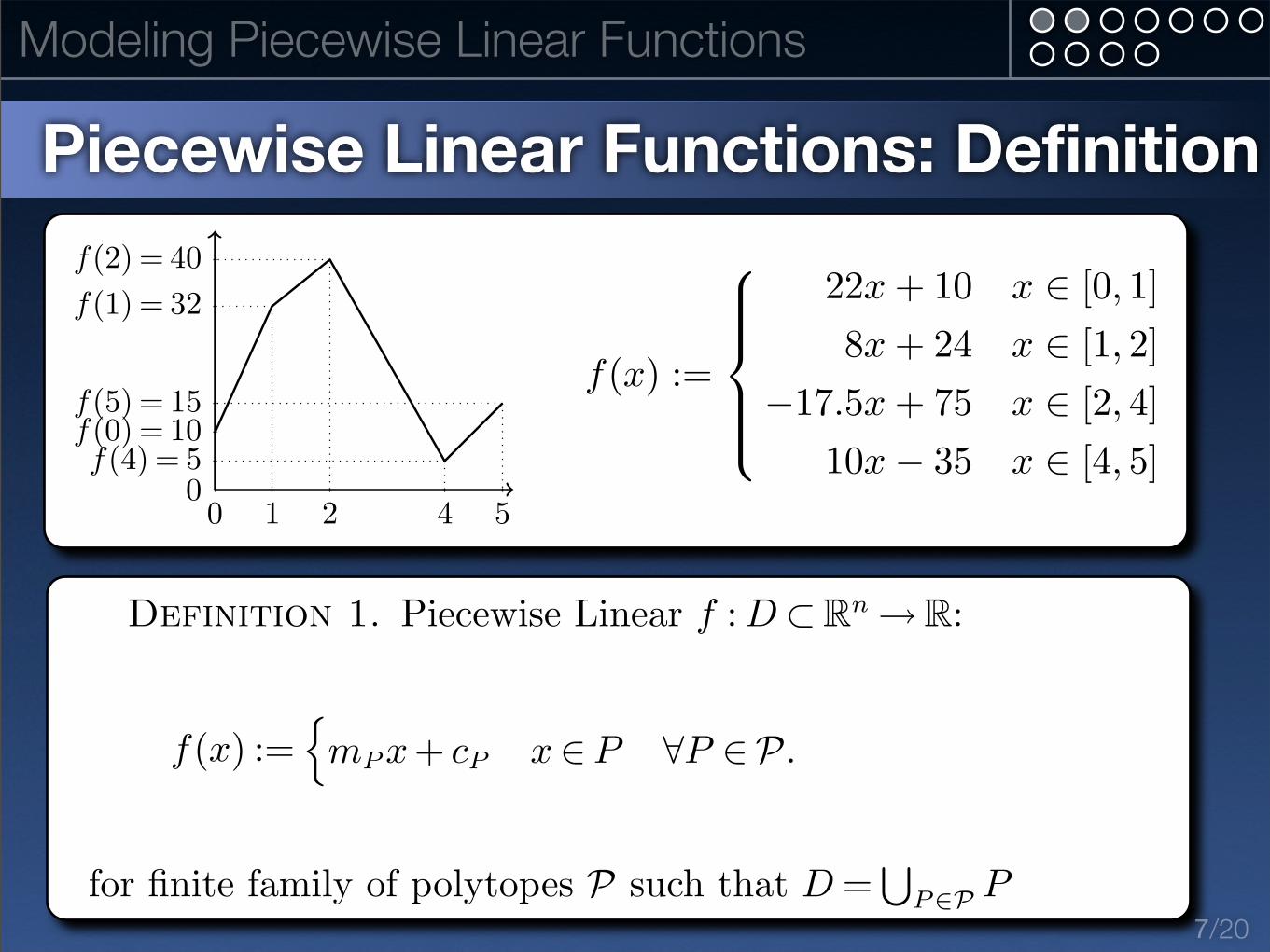
Definition 1. Piecewise Linear f : D ⊂Rn →R:

f(x) :={

mP x+ cP x∈ P ∀P ∈P.

for finite family of polytopes P such that D =⋃

P∈PP

/20


Piecewise Linear Functions: Definition

7

0 1 2 4 5

f(4) = 50

f(0) = 10

f(1) = 32

f(2) = 40

f(5) = 15

/20


Epigraph of PLF is Union of Polyhedra

8

= ∪ ∪ ∪⋃

∈P

( )

epi(f) = C+

n+

⋃

P∈P

conv(

{(v, f(v))}v∈V (P )

)

= C+

n+

⋃

P∈P

conv(

{(v, mP v + cP )}v∈V (P )

)

C+

n := {(0, z) ∈ n × : z ≥ 0}, V (P ) := vertices of P .

/20


Convex Combination Models

9

d0 d1 d2 d3 d4

f(d3)0

f(d0)

f(d1)

f(d2)

f(d4)

/20


Disaggregated Conv. Comb. (DCC)

Croxton et al. (2003a), Jeroslow (1987), Jeroslow and

Lowe (1984), Lowe (1984), Meyer (1976) and Sherali (2001)

10

∑

P∈P

∑

v∈V (P )

λP,vv = x,∑

P∈P

∑

v∈V (P )

λP,v (mP v + cP )≤ z

λP,v ≥ 0 ∀P ∈P, v ∈ V (P ),∑

v∈V (P )

λP,v = yP ∀P ∈P

∑

P∈P

yP = 1, yP ∈ {0,1} ∀P ∈P.

/20


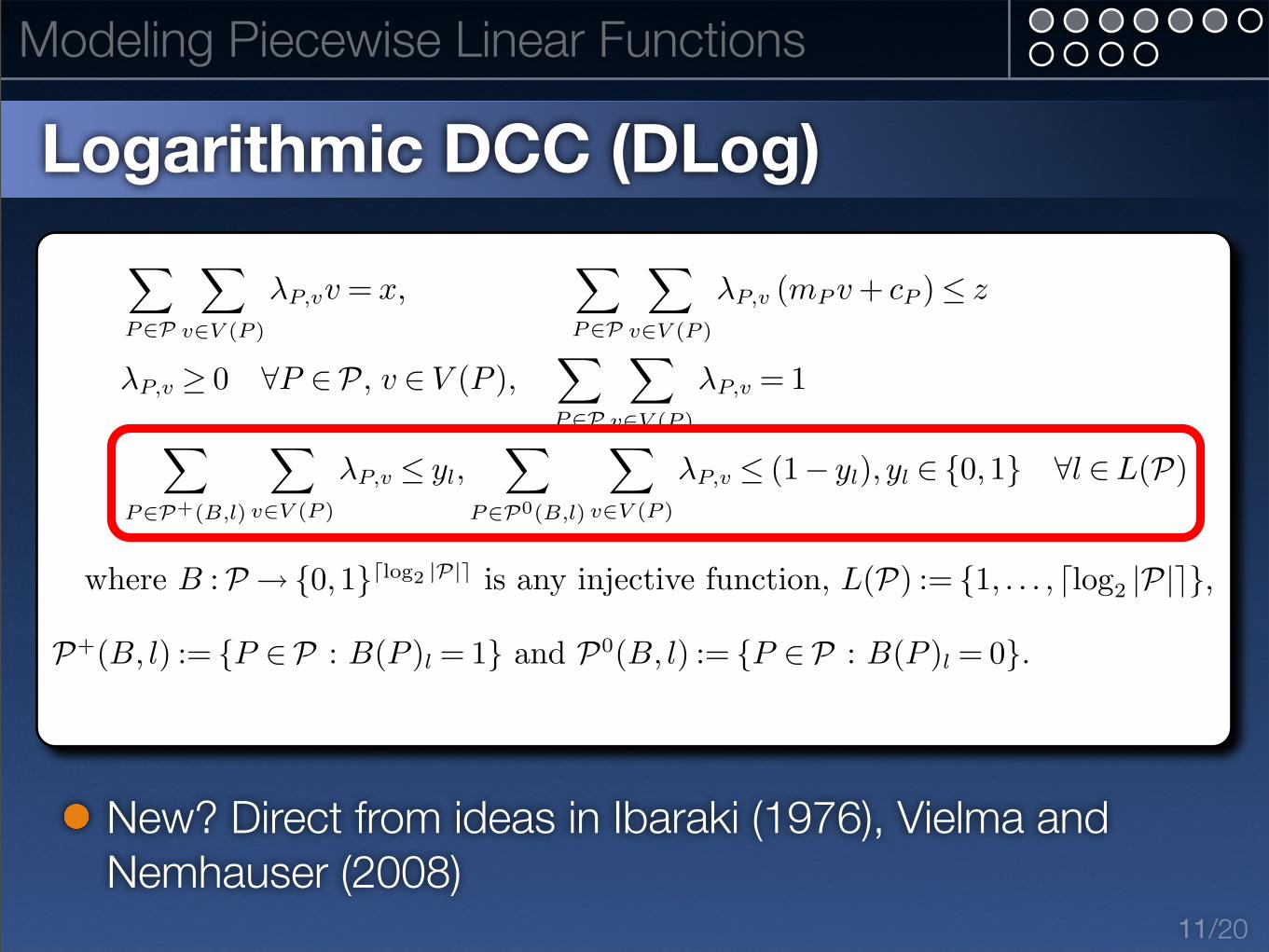
Logarithmic DCC (DLog)

New? Direct from ideas in Ibaraki (1976), Vielma and

Nemhauser (2008)11

∑

P∈P

∑

v∈V (P )

λP,vv = x,∑

P∈P

∑

v∈V (P )

λP,v (mP v + cP )≤ z

λP,v ≥ 0 ∀P ∈P, v ∈ V (P ),∑

P∈P

∑

v∈V (P )

λP,v = 1

∑

P∈P+(B,l)

∑

v∈V (P )

λP,v ≤ yl,∑

P∈P0(B,l)

∑

v∈V (P )

λP,v ≤ (1− yl), yl ∈ {0,1} ∀l ∈L(P)

where B :P → {0,1}⌈log2 |P|⌉ is any injective function, L(P) := {1, . . . , ⌈log2 |P|⌉},

P+(B, l) := {P ∈P : B(P )l = 1} and P0(B, l) := {P ∈P : B(P )l = 0}.

∑

v∈V(P)

λvv = x,

∑

v∈V(P)

λv (mP v + cP )≤ z

λv ≥ 0 ∀v ∈ V(P),∑

v∈V(P)

λv = 1

λv ≤∑

P∈P(v)

yP ∀v ∈ V(P),

∑

P∈P

yP = 1, yP ∈ {0,1} ∀P ∈P,

/20


Convex Combination (CC)

Dantzig (1963, 1960), Garfinkel and Nemhauser (1972), Jeroslow and Lowe (1985), Keha

et al. (2004), Lee and Wilson (2001), Lowe (1984), Nemhauser and Wolsey (1988),

Padberg (2000) and Wilson (1998)12

where P(v) := {P ∈P : v ∈ P}. This

/20


Logarithmic Conv. Comb. (Log)

Requires Independent Branching Scheme.

Vielma and Nemhauser (2008).

13

∑

v∈V(P)

λvv = x,

∑

v∈V(P)

λv (mP v + cP )≤ z

λv ≥ 0 ∀v ∈ V(P),∑

v∈V(P)

λv = 1

∑

v∈Ls

λv ≤ ys,

∑

v∈Rs

λv ≤ (1− ys), ys ∈ {0,1} ∀s∈ S.

/20


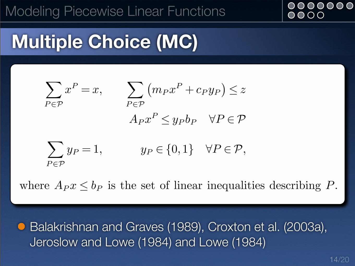
Multiple Choice (MC)

Balakrishnan and Graves (1989), Croxton et al. (2003a),

Jeroslow and Lowe (1984) and Lowe (1984)

14

∑

P∈P

xP = x,∑

P∈P

(mP xP + cP yP

)

≤ z

AP xP ≤ yP bP ∀P ∈P

∑

P∈P

yP = 1, yP ∈ {0,1} ∀P ∈P,

where AP x ≤ bP is the set of linear inequalities describing P . This

/20


Incremental or Delta (Inc)

Similar for multivariate functions.

Croxton et al. (2003a), Dantzig (1963, 1960), Keha et al.

(2004), Markowitz and Manne (1957), Padberg (2000),

Sherali (2001), Vajda (1964) and Wilson (1998).15

d0 d1 d2 d3 d4

f(d3)0

f(d0)

f(d1)

f(d2)

f(d4)

d0 +K∑

k=1

δk (dk − dk−1) = x

f(d0)+K∑

k=1

δk (f(dk)− f(dk−1))≤ z

δ1 ≤ 1, δK ≥ 0, δk+1 ≤ yk ≤ δk,

yk ∈ {0,1} ∀k ∈ {1, . . . ,K − 1}.

/20


Strength of the Models

All models give the same LP relaxation bound:

LP relaxation is model of lower convex

envelope (Sharp).

In the absence of other constraints:

All models except for CC have integral vertices

(Locally Ideal).

16

Instances

Transportation problems (10x10 & 5x2).

Univariate: Concave Separable Objective.

Multivariate: Multi-commodity function.

Functions are affine in k segments or in a

k x k grid triangulation (100 instances per

each k=4, 8, 16, 32).

Solver: CPLEX 11 on 2.4Ghz machine.

/20


Instances and Solvers

17

0 1 20

1

2

/20


Univariate Case (Separable)

18

1

10

100

1000

10000

DCC CC MC Inc SOS2 DLog Log

Average Time Solve [s]

Formulation

48

1632

/20


Multivariate Case (Non-Separable)

19

1

10

100

1000

10000

DCC CC MC Inc DLog Log

Average Time Solve [s]

Formulation

4x48x8

16x16

/20

Conclusions

Conclusions and Other Results

Suggestions

For small k use MC or Inc

instead of DCC or CC.

For large k use DLog or

Log.

DLog, DCC and MC can

also be also used for Lower

Semicontinuous Functions.

20

x

y

Mixed Integer Programming Models for Non-Separable Piecewise Linear Cost Functions

Documents

Transcript of Mixed Integer Programming Models for Non-Separable Piecewise Linear Cost Functions