Mixed H2/H∞ Tracking Control withConstraints for Single Quadcopter Carrying

a Cable-suspended Payload

Minhuan Guo ∗ , Yan Su ∗∗ , Dongbing Gu ∗∗∗

∗Nanjing University of Science and Technology, Nanjing, 210094,China (e-mail: 312012201@njust.edu.cn).

∗∗Nanjing University of Science and Technology, Nanjing, 210094,China (suyan@mail.njust.edu.cn).

∗∗∗ School of Computer Science and Electronic Engineering, Universityof Essex, Wivenhoe Park, Colchester, CO4 3SQ, UK, (e-mail:

dgu@essex.ac.uk)

Abstract: In order to control a single quadcopter with a cable-suspended payload to follow thedesired trajectory, a mixed H2/H∞ controller with constraints is developed. Firstly, the Euler-Lagrange dynamic model is built and linearized. Then the extended model for path trackingproblem is designed. Based on linear matrix inequality (LMI), state feedback controller H2 andH∞ with constraints is illustrated. Aiming to maintain a good balance in transient behaviors andfrequency-domain performance, the mixed controller is presented. Finally, the control strategiesare utilized in a simulation test and the result validates the proposed method.

Keywords: aircraft control, H2 norm, H∞ norm, linear matrix inequality, Lyapunov function,state control.

1. INTRODUCTION

Nowadays unmanned aerial vehicles (UAVs) are gainingmore and more popularity in many possible applicationsincluding search and rescue, disaster relief operations,environmental monitoring, wireless surveillance networks,and cooperative manipulation. Lifting and transportationof a cable-suspended payload by a quadcopter is a chal-lenging and useful issue.

Much literature has been published around this topic.Cruz and Fierro (2014) addresses the problem of liftingfrom the ground a cable-suspended load by a quadrotoraerial vehicle, where the mass of the load is unknown.Faust et al. (2013) presents a motion planning method forgenerating trajectories with minimal residual oscillationsfor rotorcraft carrying a suspended load and completesthe multi-waypoint flight in the cluttered environment.Palunko et al. (2012) uses a high-level planner to providedesired waypoints and utilize a dynamic programmingapproach to generate the swing-free trajectory to keep theminimum load swing. Sreenath et al. (2013) establishesa differentially-flat hybrid system for the quadrotor-loadsystem and develops a nonlinear geometric controller toenable tracking of outputs. As for the controller design, inDe Crousaz et al. (2014), the iLQG method is applied tothe hybrid system and the aggressive controller is designedfor controlling the payload to pass through a small window.Alothman et al. (2015) proposes a linear quadratic regula-tor (LQR) for lifting and transporting the load. The singlesituation is extended to multi-vehicles in Sreenath andKumar (2013), which addresses the problem of cooperative

transportation of a cable-suspended payload by multiplequadcopters.

This paper presents a mixed H2/H∞ tracking controllerbased on linear matrix inequality (LMI). Basically, prob-lems around H2 and H∞ control are studied widely.Apkarian et al. (2001), Zhai et al. (2003), and Filasovaet al. (2016) describe the framework for H2 and H∞performance based on linear matrix inequality. It is knownthat while H∞ control design is mainly concerned withfrequency-domain performance, and does not guaranteegood transient behaviors for the closed-loop system, H2

control design gives more suitable performance on sys-tem transient behaviors Nonami and Sivrioglu (1996).The proposed method tries to maintain a good balanceon transient behavior and frequency-domain performance.Besides, the constraints for the inputs and outputs are alsoconsidered in this paper.

The remaining parts of this paper are organized as follows.In section 2, the nonlinear and linear models are described.In section 3, the extended model for tracking problemis given and the mixed H2/H∞ controller is presented.In section 4, the proposed method is developed in asimulation test and the results are analyzed. Finally, a briefconclusion is provided.

2. MODEL DESCRIPTION

2.1 System and Notations

The full system is presented in Fig. 1, including the inertialframe, intermediate frame, body-fixed frame, vertical andhorizontal forces generated by each propeller and swing

angles of the rope with respect to the intermediate frame.In order to simplify the problem, some reasonable hypothe-ses are given as follows:

(1) The quadcopter is considered as a symmetrical rigidbody.

(2) The payload is considered as a point mass and isattached at the center of the quadcopter.

(3) The cable tension is always non-zero.(4) The air drag of the propellers is negligible.

xe ye

ze

xy

z

P

P’

Q

xb

yb

zb

f1z

f1h

f3zf3h

f2z

f2h

f4z

f4h

α

β

Fig. 1. Single quadcopter with a cable-suspended payload

Partial symbols and acronyms used in this paper are lisedin table 1.

Table 1. Symbols and Definitions

Symbol Description

Se : xeyeze Inertial frameS : xyz Intermediate frame: translate Se

to the center of the quadcopterSb : xbybzb Body-fixed frameEi ∈ R3, i = 1, 2, 3 Unit orthogonal vectors of Se

ei ∈ R3, i = 1, 2, 3 Unit orthogonal vectors of Sb

η = [φ, θ, ψ]T ∈ R3 Euler angles of quadcopter definedin Z − Y −X

Te2b ∈ R3×3 Transformation matrix from Se to Sb

Ω ∈ R3 Angular velocity of quadcopter in Sb

mQ = 0.55kg Mass of the quadcoptermP = 0.05kg Mass of the payloadIQ ∈ R3 Inertial matrix of the quadcopter

with respect to Sb

ξQ ∈ R3 Position of the center of quadcopter in Se

ξP ∈ R3 Position of the payload in Se

Lr = 0.5m Length of the ropeLQ = 0.17m Length of the quadcopter armα, β ∈ R Angles of the rope with respect to Sρ ∈ R3 Unit vector from the payload to

the attached pointfiz ,fih ∈ R3 Vertial and horizontal forces generated

by ith propeller, i = 1, 2, 3, 4kF , kM ∈ R Propeller aerodynamic parameters

As illustrated in Fig. 1, the following relationships areavailable.

ρ = [−sin(β),−cos(α)cos(β), sin(α)cos(β)]T

ξP = xPE1 + yPE2 + zPE3

ξQ = ξP + Lrρ

Ω =

[1 0 −sin(θ)0 cos(φ) sin(φ)cos(θ)0 −sin(φ) cos(φ)cos(θ)

] φθψ

(1)

2.2 Euler-Lagrange Modeling

The quadcopter-payload system has 8 degrees of freedom.

Choosing q = [xP , yP , zP , α, β, φ, θ, ψ]T

as the generalizedcoordinates will not only be convenient while controllingthe trajectory of the payload but also be helpful for extend-ing to multi-vehicle situation. As a result, the Lagrangianis given by

T =1

2mP ξ

TP · ξP +

1

2mQξ

TQ · ξQ +

1

2ΩT IQΩ

U = mP gξP ·E3 +mQgξQ ·E3

L = T − U

(2)

Then the Euler-Lagrange equation is

d

dt(∂L

∂q)− ∂L

∂q= Q (3)

The generalized forces Q defined here are based on thechoice of the generalized coordinates q and the externalconservative forces

∑Fi. The force Fi consists of two

complements fiz and fih (equation (4)) which are relatedwith the angular speed ωi of ith propeller.

Fi = fiz + fih, i = 1, 2, 3, 4

fiz = kFω2i e3, i = 1, 2, 3, 4

f1h = kMω21e2

f2h = kMω22e1

f3h = −kMω23e2

f4h = −kMω24e1

(4)

where ei = Te2bEi, i = 1, 2, 3.

As seen in Fig. 1, the point where the force Fi is appliedon is the center of each propeller and the correspondingposition vector is noted as ξi seen in equation (5).

ξ1 = ξQ + LQe1

ξ2 = ξQ + LQe2

ξ3 = ξQ − LQe1

ξ4 = ξQ − LQe2

(5)

According to the principle of virtual work, the generalizedforces are given by equation (6).

Qi =

4∑j=1

∂(Fj · ξj)∂qi

, i = 1, 2, .., 8 (6)

Taking the generalized forces (detailed in (A.1)) and equa-tion (2) into equation (3), the Euler-Lagrange equation canbe rewritten in

Mq = f(q, q) (7)

where M and f(q, q) are detailed in (A.2) and (A.3)respectively.

Considering the balance situation as the equilibrium point(x0,u0), the linearized model is obtained in equation (8).

q = M−1 ∂f

∂x

∣∣∣∣x0

∆x+M−1 ∂f

∂u

∣∣∣∣u0

∆u (8)

Furthermore, equation (8) can be stated in the followingstandard state-space form.

x = Ax+Bu

y = Cx(9)

where A ∈ R16×16 and B ∈ R16×4 are detailed in(A.4)and (A.5), C = I16×16.

x =[xP , xP , yP , yP , zP , zP , α, α, β, β, φ, φ, θ, θ, ψ, ψ

]T∈

R16, u = [ω1, ω2, ω3, ω4]T ∈ R4,y ∈ R16

3. CONTROL STRATEGIES

3.1 Extended Model for Tracking Path

Taking account of the integrations of the position trackingerror, the diagram of state feedback controller is seen inFig. 2.

Pxe

P

dtxòe Plant

dx

1

s

K

x

e xdue

du

u

nu

Fig. 2. Diagram of extended state feedback controller

The desired and feasible trajectory is(xd,ud

), so the state

error is e ∈ R16 := xd − x.

The integration of the position error is∫eξP dt ∈ R3 .

The new error state is e =[eT ,

∫eTξP dt

]T∈ R19.

Therefore, equation (9) can be stated in following form oftracking error e and disturbance inputs w = un ∈ R4.

˙e = Ae+Bωw +Buδu (10)

where, A =

[A 0F 0

]∈ R19×19,F = Bω =

[B0

]∈

R19×4,Bu =

[B0

]∈ R19×4. All the states are detectable

and considered as measurement outputs. The H2, H∞ andconstraint performance outputs are as follows:

z2 = C2x+D2u

z∞ = C∞x+D∞u

zc = Ccx+Dcu

(11)

where C2, D2, C∞, D∞, Cc, Dc are appropriate weightmatrix.

As a result, equation (11) is equal to the following transferfunction matrix in terms of H2 and H∞ performances.

G =

[G11 G12

G21 G22

]=

A Bw Bu

C2 0 D2

C∞ 0 D∞

(12)

The problem of mixed H2/H∞ tracking control withconstraints is described like:

minKmix

‖Tz2u(Kmix)‖2s.t.‖Tz∞w(Kmix)‖∞ ≤ γ|ui(t)| ≤ uimax

|zci(t)| ≤ zimax

(13)

where, γ is the acceptable gain of H∞ norm, uimax andzimax are the maximum constraints. Then the feedbackcontroller is:

u = δu+ ud = Kmixe+ ud (14)

3.2 Mixed H2/H∞ LMI Control with Constraints

Lemma 1. (H2 Performance)Given an upper bound λ > 0, if there exist symmetricpositive definite matrices X2, Z and general matrix R2

satisfying

X2 = XT2 0,Z = ZT 0[

AX2 +X2AT +BuR2 +RT

2BTu ∗

BTu −I

] 0[

Z ∗X2C

T2 +RT

2DT2 X2

] 0

trZ < λ2

(15)

where state-feedback gain matrix K2 = R2X−12 . Then,

the controller stabilizes the closed-loop system and theupper bound of H2 performance index is λ.

Proof. See Apkarian et al. (2001).

Lemma 2. (H∞ Performance with Constraints)Given an upper bound γ > 0, if there exit symmetricpositive definite matrix Q∞, positive diagonal matrixU ,Y and general matrix Y∞ satisfying

Q∞ = QT∞ 0AQ∞ +Q∞A

T +BuY∞ + Y T∞B

Tu ∗ ∗

C∞Q∞ +D∞Y∞ −γI ∗BTw 0 −γI

≺ 0

[1

αU Y∞

∗ Q∞

] 0,Uii ≺ u2

imax[1

αY CcQ∞ +DcY∞

∗ Q∞

] 0,Yii ≺ z2

imax

(16)

where state-feedback gain matrix K∞ = Y∞Q−1∞ . Then,

the controller meets the constraints, robustly stabilizes theclosed-loop system and the upper bound of H∞ perfor-mance index is γ.

Proof. The proof for H∞ is seen in Filasova et al. (2016).Since K∞ = Y∞Q

−1∞ is the state feedback gain for H∞

performance, it guarantees the closed system A+BuK∞to be asymptotic stable.

Choosing V (x(t)) = ||Q−1/2∞ x(t)||22 as the Lyapunov func-

tion, we get

d

dtV (x(t)) + γ−1‖z∞(t)‖2 − γ‖w(t)‖2 ≤ 0 (17)

After integration,

V (x(t))+γ−1

∫ t

0

‖z∞(τ)‖2dτ ≤ γ∫ t

0

‖w(τ)‖2dτ+V (x(0))

(18)

Assume∫∞

0‖w(t)‖2dt ≤ wmax, equation (17) means the

state stays in the ellipsoid:

Ω(Q−1/2∞ , α) = x ∈ Rn|V (x) ≤ α (19)

where, α = γwmax + V (x(0)).Constraints for the inputs and outputs are:

maxt≥0|ui(t)|2 = max |(Y∞Q−1

∞ )ix(t)|2

≤ maxx∈Ω|(Y∞Q−1

∞ )ix|2

≤ α||(Y∞Q− 1

2∞ )i||22maxt≥0|zci(t)|2 = max |(Cc +DcY∞Q

−1∞ )ix(t)|2

≤ maxx∈Ω|(Cc +DcY∞Q

−1∞ )ix|2

≤ α||((CcQ∞ +DcY∞)Q− 1

2∞ )i||22

(20)

where, subscript i means the ith row of the matrix.Finally, equation (20) can be rewritten in the forms inequation (16). This concludes the proof.

Lemma 3. (H2/H∞ Performance with Constraints)Given upper bounds of H2 and H∞ are λ and γ respec-tively, if there exist symmetric positive definite matricesX, Z, positive diagonal matrix U ,Y and general matrixR satisfying

X = XT 0,Z = ZT 0

trZ < λ2[Z ∗

XCT2 +RTDT

2 X

] 0[

AX +XAT +BuR+RTBTu ∗

BTu −I

] 0AX +XAT +BuR+RTBT

u ∗ ∗C∞X +D∞R −γI ∗

BTw 0 −γI

≺ 0

[1

αU R

∗ X

] 0,Uii ≺ u2

imax[1

αY CcX +DcR

∗ X

] 0,Yii ≺ z2

imax

(21)

where state-feedback gain matrix Kmix = RX−1. Then,the controller meets the constraints, robustly stabilizes theclosed-loop system and the upper bound of H∞ perfor-

mance index is γ and stabilizes the closed-loop system andthe upper bound of H2 performance index is λ.

Proof. Considering that K in Lemma 1 and 2 should beconsistent, after assuming X = X2 = Q∞ and R = R2 =Y∞, equation (21) is obtained.

4. SIMULATION RESULTS

In order to check the effectiveness of the proposed con-troller, a simulation test has been implemented on Mat-lab/Simulink. Specifically, the designed controllers try tocarry the payload from the initial position (0, 0, 0) to thedesired position (−1, 1, 1.0). The test results are seen inFig. 3-7.

0 2 4 6 8 10 12

x(m

)

-2

0

2

0 2 4 6 8 10 12

y(m

)

0

1

2

time (s)0 2 4 6 8 10 12

z(m

)

0

1

2

K_H2K_H∞_CK_H2/H∞_CReference

Fig. 3. Position of the payload

As for the trajectory tracking performance in Fig. 3, H2

controller has the longest response time, whilst H∞ andHmix have a shorter and nearly close one.

0 2 4 6 8 10 12

φ(deg)

-50

0

50

0 2 4 6 8 10 12

θ(deg)

-50

0

50

time (s)0 2 4 6 8 10 12

ψ(deg)

-20

0

20

K_H2K_H∞_CK_H2/H∞_C

Fig. 4. Attitude of the quadcopter

In terms of the quadcopter’s attitude (Fig. 4), H2 hasthe most stable angular rate and H∞ has the worst

performance. In comparison, Hmix is much smoother thanH∞ and a little greater than H2.

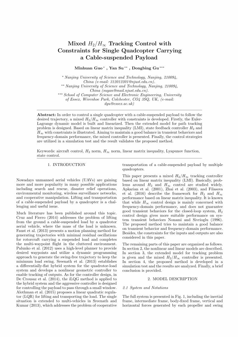
Considering the inertia of the payload, the swing angles (αand β) will not change dramatically. Seen in Fig. 5, H∞and Hmix have larger but acceptable swing angles sincethey have a shorter response time for trajectory trackingproblem.

0 2 4 6 8 10 12

α(deg)

-20

0

20

time (s)0 2 4 6 8 10 12

β(deg)

-20

0

20 K_H2K_H∞_CK_H2/H∞_C

Fig. 5. Swing angles of the cable

Fig. 6 and 7 illustrate the H2 and H∞ norm perfor-mance for these three controllers. It is obvious that Hmix

maintains a balance on transient behavior and frequencydomain performance.

0 2 4 6 8 10 120

2

4

6‖Z‖

2

time (s)0 2 4 6 8 10 12

0

5000

10000

∫‖Z‖

2dt

K_H2K_H∞_CK_H2/H∞_C

Fig. 6. H2 performance

In Fig. 6, when the quadcotor starts to carry the payloadto the desired position, the H∞ controller causes too muchoscillation which is bad for maintaining stable. However,Hmix does betther in eliminating these side effects.

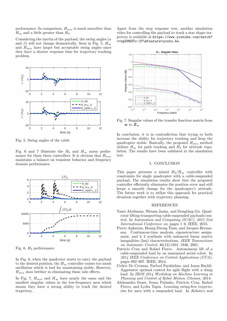
In Fig. 7, Hmix and H∞ have nearly the same and thesmallest singular values in the low-frequency area whichmeans they have a strong ability to track the desiredtrajectory.

Apart from the step response test, another simulationvideo for controlling the payload to track a star shape tra-jectory is available at https://www.youtube.com/watch?v=zpD9ROTo-2Y\&feature=youtu.be.

10-3 10-2 10-1 100 101 102 103-600

-500

-400

-300

-200

-100

0

100

K_H2K_H∞_CK_H2/H∞_C

H∞ Singular Value

Frequency (rad/s)

Sin

gula

r V

alue

s (d

B)

Fig. 7. Singular values of the transfer function matrix fromw to Z∞

In conclusion, it is in contradiction that trying to bothincrease the ability for trajectory tracking and keep thequadcopter stable. Basically, the proposed Hmix methodutilizes H∞ for path tracking and H2 for attitude regu-lation. The results have been validated in the simulationtest.

5. CONCLUSION

This paper presents a mixed H2/H∞ controller withconstraints for single quadcopter with a cable-suspendedpayload. The simulation results show that the proposedcontroller efficiently eliminates the position error and stillkeeps a smooth change for the quadcopter’s attitude.The future work is to utilize this approach for practicalsituation together with trajectory planning.

REFERENCES

Yaser Alothman, Wesam Jasim, and Dongbing Gu. Quad-rotor lifting-transporting cable-suspended payloads con-trol. In Automation and Computing (ICAC), 2015 21stInternational Conference on, pages 1–6. IEEE, 2015.

Pierre Apkarian, Hoang Duong Tuan, and Jacques Bernus-sou. Continuous-time analysis, eigenstructure assign-ment, and h 2 synthesis with enhanced linear matrixinequalities (lmi) characterizations. IEEE Transactionson Automatic Control, 46(12):1941–1946, 2001.

Patricio Cruz and Rafael Fierro. Autonomous lift of acable-suspended load by an unmanned aerial robot. In2014 IEEE Conference on Control Applications (CCA),pages 802–807. IEEE, 2014.

Cedric De Crousaz, Farbod Farshidian, and Jonas Buchli.Aggressive optimal control for agile flight with a slungload. In IROS 2014 Workshop on Machine Learning inPlanning and Control of Robot Motion. Citeseer, 2014.

Aleksandra Faust, Ivana Palunko, Patricio Cruz, RafaelFierro, and Lydia Tapia. Learning swing-free trajecto-ries for uavs with a suspended load. In Robotics and

Automation (ICRA), 2013 IEEE International Confer-ence on, pages 4902–4909. IEEE, 2013.

Anna Filasova et al. On enhanced mixed h2/h∞ designconditions for control of linear time-invariant systems.In Carpathian Control Conference (ICCC), 2016 17thInternational, pages 384–389. IEEE, 2016.

Kenzo Nonami and SELIM Sivrioglu. Active vibrationcontrol using lmi-based mixed h2/h∞ state and outputfeedback control with nonlinearity. In Decision and Con-trol, 1996., Proceedings of the 35th IEEE Conference on,volume 1, pages 161–166. IEEE, 1996.

Ivana Palunko, Rafael Fierro, and Patricio Cruz. Trajec-tory generation for swing-free maneuvers of a quadro-tor with suspended payload: A dynamic programmingapproach. In Robotics and Automation (ICRA), 2012IEEE International Conference on, pages 2691–2697.IEEE, 2012.

Koushil Sreenath and Vijay Kumar. Dynamics, controland planning for cooperative manipulation of payloadssuspended by cables from multiple quadrotor robots. rn,1(r2):r3, 2013.

Koushil Sreenath, Taeyoung Lee, and Vijay Kumar. Ge-ometric control and differential flatness of a quadrotoruav with a cable-suspended load. In 52nd IEEE Confer-ence on Decision and Control, pages 2269–2274. IEEE,2013.

Guisheng Zhai, Shinichi Murao, Naoki Koyama, and Masa-haru Yoshida. Low order h controller design: An lmi ap-proach. In European Control Conference (ECC), 2003,pages 3070–3075. IEEE, 2003.

Appendix A. SOME RESULTS

Generalized forces:Q1 =kM (ω2

2 − ω24)CθCψ + Cφ(kF (ω2

1 + ω22 + ω2

3 + ω24)CψSθ

+ kM (−ω21 + ω2

3)Sψ) + Sφ(kM (ω21 − ω2

3)CψSθ + kF (ω21 + ω2

2 + ω23 + ω2

4)Sψ)

Q2 =−kF (ω21 + ω2

2 + ω23 + ω2

4)CψSφ+ kM ((ω22 − ω2

4)Cθ + (ω21 − ω2

3)SθSφ)Sψ

+ Cφ(kM (ω21 − ω2

3)Cψ + kF (ω21 + ω2

2 + ω23 + ω2

4)SθSψ)

Q3 =kM (−ω22 + ω2

4)Sθ + Cθ(kF (ω21 + ω2

2 + ω23 + ω2

4)Cφ+ kM (ω21 − ω2

3)Sφ)

Q4 =Lr(Sα(−kF (ω21 + ω2

2 + ω23 + ω2

4)CψSφ+ kM ((ω22 − ω2

4)Cθ + (ω21 − ω2

3)SθSφ)Sψ

+ Cφ(kM (ω21 − ω2

3)Cψ + kF (ω21 + ω2

2 + ω23 + ω2

4)SθSψ))

+ Cα(Cβ(kM (−ω22 + ω2

4)Sθ + Cθ(kF (ω21 + ω2

2 + ω23 + ω2

4)Cφ+ kM (ω21 − ω2

3)Sφ))

− Sβ(kM (ω22 − ω2

4)CθCψ + Cφ(kF (ω21 + ω2

2 + ω23 + ω2

4)CψSθ + kM (−ω21 + ω2

3)Sψ)

+ Sφ(kM (ω21 − ω2

3)CψSθ + kF (ω21 + ω2

2 + ω23 + ω2

4)Sψ))))

Q5 =LrSα(−Sβ(kM (−ω22 + ω2

4)Sθ + Cθ(kF (ω21 + ω2

2 + ω23 + ω2

4)Cφ

+ kM (ω21 − ω2

3)Sφ))− Cβ(kM (ω22 − ω2

4)CθCψ + Cφ(kF (ω21 + ω2

2 + ω23 + ω2

4)CψSθ

+ kM (−ω21 + ω2

3)Sψ) + Sφ(kM (ω21 − ω2

3)CψSθ + kF (ω21 + ω2

2 + ω23 + ω2

4)Sψ)))

Q6 =kFLQ(ω22 − ω2

4)

Q7 =LQ(−kF (ω21 − ω2

3)Cφ+ kM (−ω21 + ω2

2 − ω23 + ω2

4)Sφ)

Q8 =LQ(kF (−ω22 + ω2

4)Sθ + Cθ(kM (ω21 − ω2

2 + ω23 − ω2

4)Cφ+ kF (−ω21 + ω2

3)Sφ))

(A.1)

Matrix M:

M =

[M11 05×3

03×5 M22

](A.2)

where, M11 and M22 are defined as follows:

M11 =

mP +mQ 0 0 0 −LrmQCβ

0 mP +mQ 0 LrmQCβSα LrmQCαSβ0 0 mP +mQ LrmQCαCβ −LrmQSαSβ0 LrmQCβSα LrmQCαCβ L2

rmQCβ2 0

−LrmQCβ LrmQCαSβ −LrmQSαSβ 0 L2rmQ

M22 =

Ix 0 −IxSθ0 IyC

2φ+ IzS2φ (Iy − Iz)CθCφSφ

−IxSθ (Iy − Iz)CθCφSφ IxS2θ + C2θ(IzC

2φ+ IyS2φ)

Definitions of function f(q, q):

f1(q, q) = kMω22C[θ]C[ψ]− kMω2

4C[θ]C[ψ] + kFω21C[φ]C[ψ]S[θ] + kFω

22C[φ]C[ψ]S[θ]

+ kFω23C[φ]C[ψ]S[θ] + kFω

24C[φ]C[ψ]S[θ] + kMω

21C[ψ]S[θ]S[φ]

− kMω23C[ψ]S[θ]S[φ]− kMω2

1C[φ]S[ψ] + kMω23C[φ]S[ψ] + kFω

21S[φ]S[ψ]

+ kFω22S[φ]S[ψ] + kFω

23S[φ]S[ψ] + kFω

24S[φ]S[ψ]− LrmQS[α]S[β]α2

+ 2LrmQC[α]C[β]αβ − LrmQS[α]S[β]β2

f2(q, q) = −kFω21C[ψ]S[φ]− kFω2

2C[ψ]S[φ]− kFω23C[ψ]S[φ]− kFω2

4C[ψ]S[φ]

+ kMω22C[θ]S[ψ]− kMω2

4C[θ]S[ψ] + kMω21S[θ]S[φ]S[ψ]− kMω2

3S[θ]S[φ]S[ψ]

+ C[φ](kM (ω21 − ω2

3)C[ψ] + kF (ω21 + ω2

2 + ω23 + ω2

4)S[θ]S[ψ])− LrmQC[α]α2

f3(q, q) = −gmP − gmQ + kFω21C[θ]C[φ] + kFω

22C[θ]C[φ] + kFω

23C[θ]C[φ]

+ kFω24C[θ]C[φ]− kMω2

2S[θ] + kMω24S[θ] + kMω

21C[θ]S[φ]− kMω2

3C[θ]S[φ]

+ LrmQC[β]S[α]α2 + 2LrmQC[α]S[β]αβ + LrmQC[β]S[α]β2

f4(q, q) = Lr(S[α](−kF (ω21 + ω2

2 + ω23 + ω2

4)C[ψ]S[φ] + kM ((ω22 − ω2

4)C[θ]

+ (ω21 − ω2

3)S[θ]S[φ])S[ψ] + C[φ](kM (ω21 − ω2

3)C[ψ]

+ kF (ω21 + ω2

2 + ω23 + ω2

4)S[θ]S[ψ]))− C[α](C[β](gmQ + kM (ω22 − ω2

4)S[θ]

− C[θ](kF (ω21 + ω2

2 + ω23 + ω2

4)C[φ] + kM (ω21 − ω2

3)S[φ]))

+ S[β](kM (ω22 − ω2

4)C[θ]C[ψ] + C[φ](kF (ω21 + ω2

2 + ω23 + ω2

4)C[ψ]S[θ]

+ kM (−ω21 + ω2

3)S[ψ]) + S[φ](kM (ω21 − ω2

3)C[ψ]S[θ]

+ kF (ω21 + ω2

2 + ω23 + ω2

4)S[ψ]))) + LrmQC[α]S[α]β2)

f5(q, q) = −LrS[α](S[β](−gmQ − kM (ω22 − ω2

4)S[θ] + C[θ](kF (ω21 + ω2

2 + ω23 + ω2

4)C[φ]

+ kM (ω21 − ω2

3)S[φ])) + C[β](kM (ω22 − ω2

4)C[θ]C[ψ]

+ C[φ](kF (ω21 + ω2

2 + ω23 + ω2

4)C[ψ]S[θ] + kM (−ω21 + ω2

3)S[ψ])

+ S[φ](kM (ω21 − ω2

3)C[ψ]S[θ] + kF (ω21 + ω2

2 + ω23 + ω2

4)S[ψ])) + 2LrmQC[α]αβ)

f6(q, q) =1

2(2kFLQ(ω2

2 − ω24)− (Iyy− Izz)S[2φ]θ2 + 2C[θ](Ixx

+ (Iyy− Izz)C[2φ])θψ + (Iyy− Izz)C[θ]2S[2φ]ψ2)

f7(q, q) =1

8(−8kFLQω

21C[φ] + 8kFLQω

23C[φ]− 8kMLQω

21S[φ] + 8kMLQω

22S[φ]

− 8kMLQω23S[φ] + 8kMLQω

24S[φ] + 8(Iyy− Izz)S[2φ]θφ

− 8C[θ](Ixx + (Iyy− Izz)C[2φ])φψ + 4IxxS[2θ]ψ2 − 2IyyS[2θ]ψ2 − 2IzzS[2θ]ψ2

+ IyyS[2(θ − φ)]ψ2 − IzzS[2(θ − φ)]ψ2 + IyyS[2(θ + φ)]ψ2 − IzzS[2(θ + φ)]ψ2)

f8(q, q) = LQ(kF (−ω22 + ω2

4)S[θ] + C[θ](kM (ω21 − ω2

2 + ω23 − ω2

4)C[φ]

+ kF (−ω21 + ω2

3)S[φ])) + (Iyy− Izz)C[φ]S[θ]S[φ]θ2

− (Iyy− Izz)C[θ]2S[2φ]φψ + C[θ]θ((Ixx + (−Iyy + Izz)C[2φ])φ

+ (−2Ixx + Iyy + Izz + (−Iyy + Izz)C[2φ])S[θ]ψ)

(A.3)

Linearized model:

A =

0 1.0 0 0 0 0 0 0 0 0 0 0 0 0 0 00 0 0 0 0 0 0 0 −9.8 0 0 0 −2.6 · 10−15 0 0 00 0 0 1.0 0 0 0 0 0 0 0 0 0 0 0 00 0 0 0 0 0 9.8 0 0 0 4.3 · 10−15 0 0 0 0 00 0 0 0 0 1.0 0 0 0 0 0 0 0 0 0 00 0 0 0 0 0 6.0 · 10−16 0 0 0 6.0 · 10−16 0 0 0 0 00 0 0 0 0 0 0 1.0 0 0 0 0 0 0 0 00 0 0 0 0 0 −21.0 0 0 0 −21.0 0 0 0 0 00 0 0 0 0 0 0 0 0 1.0 0 0 0 0 0 00 0 0 0 0 0 0 0 −21.0 0 0 0 −21.0 0 0 00 0 0 0 0 0 0 0 0 0 0 1.0 0 0 0 00 0 0 0 0 0 0 0 0 0 0 0 0 0 0 00 0 0 0 0 0 0 0 0 0 0 0 0 1.0 0 00 0 0 0 0 0 0 0 0 0 0 0 0 0 0 00 0 0 0 0 0 0 0 0 0 0 0 0 0 0 1.00 0 0 0 0 0 0 0 0 0 0 0 0 0 0 0

(A.4)

B =

0 0 0 00 −1.7 · 10−19 0 1.7 · 10−19

0 0 0 0−7.1 · 10−19 −4.3 · 10−19 −1.9 · 10−19 −4.3 · 10−19

0 0 0 07.0 · 10−3 7.0 · 10−3 7.0 · 10−3 7.0 · 10−3

0 0 0 05.8 · 10−4 9.3 · 10−19 −5.8 · 10−4 9.3 · 10−19

0 0 0 00 −5.8 · 10−4 0 5.8 · 10−4

0 0 0 00 0.31 0 −0.310 0 0 0

−0.25 0 0.25 00 0 0 0

5.9 · 10−3 −5.9 · 10−3 5.9 · 10−3 −5.9 · 10−3

(A.5)