15.660 Strategic Human Resource Management MIT Sloan School of Management.

Electronic copy available at: http://ssrn.com/abstract=2258716
MIT Sloan School of Management
MIT Sloan School Working Paper 5001-13
Risk Disparity
Mark Kritzman
© Mark Kritzman
All rights reserved. Short sections of text, not to exceed two paragraphs, may be quoted with-out explicit permission, provided that full credit including © notice is given to the source.
This paper also can be downloaded without charge from theSocial Science Research Network Electronic Paper Collection:
http://ssrn.com/abstract=2258716
Electronic copy available at: http://ssrn.com/abstract=2258716

Electronic copy available at: http://ssrn.com/abstract=2258716
Risk Disparity
This Version: April 30, 2013
Mark Kritzman
Windham Capital Management and MIT Sloan
Abstract
Policy portfolios are a fixture of institutional investment management, but they may not serve the purposes for which they are intended. A policy portfolio serves primarily as an expression of an investor’s return and risk preferences. Secondarily, it serves as a benchmark for determining the success or failure of active management. A clearly defined and easily replicable policy portfolio may indeed provide a useful gauge for judging active management, but it is a poor reflection of investor preferences. Peter Bernstein [2003 and 2007] raised this issue philosophically, arguing that a policy portfolio’s risk profile was inconstant and that it changed more radically and frequently than the typical investor’s risk preferences. He went on to propose that investors manage their portfolios opportunistically rather than rigidly, but he did not provide specific guidance. This article offers empirical evidence of the inter-temporal disparity of a policy portfolio’s risk profile, and it proposes a simple framework for addressing this deficiency.

Electronic copy available at: http://ssrn.com/abstract=2258716
2
Risk Disparity1
Mark Kritzman
Policy portfolios are a fixture of institutional investment management, but they may not serve
the purposes for which they are intended. A policy portfolio serves primarily as an expression
of an investor’s return and risk preferences. Secondarily, it serves as a benchmark for
determining the success or failure of active management. A clearly defined and easily
replicable policy portfolio may indeed provide a useful gauge for judging active management,
but it is a poor reflection of investor preferences. Peter Bernstein [2003 and 2007] raised this
issue philosophically arguing that a policy portfolio’s risk profile was inconstant and that it
changed more radically and frequently than the typical investor’s risk preferences. He went on
to propose that investors manage their portfolios opportunistically rather than rigidly, but he
did not provide specific guidance. This article offers empirical evidence of the inter-temporal
disparity of a policy portfolio’s risk profile, and it proposes a simple framework for addressing
this deficiency.
1 I thank Juan Vargas for computational assistance and Timothy Adler, William Kinlaw, Yuanzhen Li, and David Turkington for helpful comments.

3
What Do Investors Want?
Investors typically seek to grow their assets and to limit exposure to significant drawdowns
along the way. Unfortunately, these two goals conflict with each other. Policy portfolios serve
as an expression of how investors balance these conflicting goals. The usual process by which
investors achieve this balance is to estimate the expected returns, risk, and correlations of
major asset classes and then to select a blend that offers the desired distribution of possible
outcomes. Typically, investors do not examine the entire distribution. Instead, they summarize
the distribution by its mean and standard deviation, assuming that returns are approximately
log-normally distributed. Given this information and assumption, investors estimate the
likelihood of various outcomes such as achieving a target growth rate or avoiding a drawdown
of a certain magnitude.2 They then select a portfolio of asset classes that best meets their
objectives, given their current outlook for expected returns, risk, and correlations.3
The problem with this approach is that the return distribution implied by a particular
portfolio at one point in time may be quite different at another point in time – and investors
want the distribution, not the portfolio. The portfolio is simply a means to an end. The solution
to the problem, therefore, is to revise the portfolio as needed to preserve the desired return
2 Of course, investors could refine this approach by considering higher moments or other features of the return distribution. See, for example, Cremers, J.H., M. Kritzman, and S. Page [2005]. 3 This approach assumes that asset classes are properly defined, which would require them to be intrinsically homogeneous and extrinsically heterogeneous. Alternatively, investors may allocate across factors and then map these factors onto the appropriate investment vehicles.

4
distribution, or at least, to give the next best distribution – in other words to replace a rigid
policy portfolio with a flexible investment policy.
Historically, investors have avoided portfolio revisions either because it was too
expensive to do so, or because they lacked confidence they could do so successfully. These two
impediments now pose less of a challenge as they might have in the past. It is now relatively
inexpensive to change exposure to asset classes or risk factors, given the proliferation of ETF’s,
index funds, and index futures. And evidence, which I will later present, together with theory,
suggests that investors may be able to anticipate macro-inefficiencies.4
Evidence of Inter-temporal Risk Disparity
Let’s consider the portfolio depicted in Exhibit 1, which is intended to represent a policy
portfolio for a typical institutional investor.
4 Paul A. Samuelson [1998] offered a theoretical argument in support of macro-inefficiency. What is now known as the Samuelson dictum states that markets are relatively micro-efficient because a smart investor who spots mispriced securities trades to exploit the inefficiency and by so doing corrects it. However, when an aggregation of securities such as an asset class is mispriced and a smart investor trades to exploit it, his actions are insufficient to revalue the entire asset class. Macro-inefficiencies typically require an exogenous shock to jolt many investors to trade in concert in order to revalue an entire asset class. Hence, macro-inefficiencies persist sufficiently long for investors to act upon them.

5
Exhibit 1: Hypothetical Institutional Portfolio5
Exhibit 2 shows the annual volatility of this portfolio based on overlapping monthly
returns, beginning January 1998 and ending February 2013.
5 I use the following indexes as proxies for the indicated asset classes: US large cap – S&P 500; US small cap – Russell 2000; EAFE equity – MSCI equity; emerging market equity – MSCI EM; US Treasuries – Barcap US Treasuries all maturities, US credit – Barcap US credit all maturities; REITS – NAREIT; and private equity – LPX.

6
Exhibit 2: Annualized Portfolio Volatility
January 1998 through February 2013
Exhibit 2 clearly reveals the inter-temporal disparity of annual portfolio volatility.
Although average portfolio volatility was 10.79%, it ranged from a low of 3.15% as of the 12
months ending May 2007 to a high of 27.81% as of August 2009. These volatility differences
imply stark differences in exposure to loss, even assuming the portfolio’s expected return
remains constant.6 Exhibit 3 shows the likelihood of various losses as of the end of a one-year
horizon, while Exhibit 4 shows the likelihood of losses within a one-year horizon.7
6 For purposes of this analysis, I assume that the portfolio’s long-term growth rate remains constant at 6.21%, which corresponds to an arithmetic average of 6.75%. These are the values that occurred for this portfolio for the period from January 1998 through February 2013. 7 The likelihood of a within-horizon loss is given by a first passage probability as follows:
P = N[(ln(1+L)-µT)/(T)] + N[(ln(1+L)+µT)/( T)] (1+L)2µ/^2
, where P = probability, L = loss, µ = expected return,
=standard deviation, T = time horiozon, and N() = cumulative normal distribution function. See, for example, Karlin, S., and H. Taylor [1975].
0%
5%
10%
15%
20%
25%
30%
De
c-9
7
De
c-9
8
De
c-9
9
De
c-0
0
De
c-0
1
De
c-0
2
De
c-0
3
De
c-0
4
De
c-0
5
De
c-0
6
De
c-0
7
De
c-0
8
De
c-0
9
De
c-1
0
De
c-1
1
De
c-1
2
7
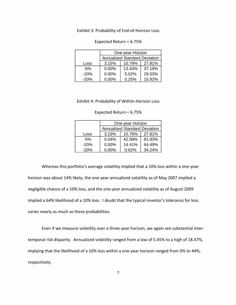
Exhibit 3: Probability of End-of-Horizon Loss
Expected Return = 6.75%
Exhibit 4: Probability of Within-Horizon Loss
Expected Return = 6.75%
Whereas this portfolio’s average volatility implied that a 10% loss within a one-year
horizon was about 14% likely, the one-year annualized volatility as of May 2007 implied a
negligible chance of a 10% loss, and the one-year annualized volatility as of August 2009
implied a 64% likelihood of a 10% loss. I doubt that the typical investor’s tolerance for loss
varies nearly as much as these probabilities.
Even if we measure volatility over a three-year horizon, we again see substantial inter-
temporal risk disparity. Annualized volatility ranged from a low of 5.45% to a high of 18.47%,
implying that the likelihood of a 10% loss within a one-year horizon ranged from 0% to 44%,
respectively.
One-year Horizon
Annualized Standard Deviation
Loss 3.15% 10.79% 27.81%
-5% 0.00% 13.43% 37.19%
-10% 0.00% 5.02% 29.53%
-20% 0.00% 0.25% 15.92%
One-year Horizon
Annualized Standard Deviation
Loss 3.15% 10.79% 27.81%
-5% 0.04% 42.58% 81.93%
-10% 0.00% 14.41% 64.49%
-20% 0.00% 0.62% 34.24%

8
How to Predict Portfolio Volatility
It is one thing to observe changes in portfolio volatility retrospectively. The challenge,
however, is to anticipate these changes. One might think that implied volatility would be an
effective precursor of portfolio volatility, because it represents a forward looking consensus
view. But this measure is limited because we can only infer implied volatility from liquid
options markets which typically do not exist for all of a portfolio’s major components. And
even if such markets did exist, this approach ignores correlations, which also change through
time and are a key driver of portfolio volatility. One might therefore consider historical
portfolio volatility, which does take correlations into account. But it too is of limited value
because, unlike implied volatility, it is backward looking, and as we observed, highly unreliable.
Instead, I propose that investors use the absorption ratio to anticipate shifts in portfolio
volatility and hence exposure to loss. This measure was introduced initially to measure and
predict systemic risk in the financial markets.8 The absorption ratio equals the fraction of the
total variance of a set of asset returns explained or “absorbed” by a fixed number of
eigenvectors, as shown in equation 1.
∑
∑
(1)
8 See, for example, Kritzman, M., Y. Li, S. Page, and R. Rigobon [2011].
9
where,
AR = Absorption ratio
N = number of assets
N = number of eigenvectors in numerator of absorption ratio
= variance of the i-th eigenvector
= variance of the j-th asset
It captures the extent to which a set of assets is unified or tightly coupled. When
assets are tightly coupled, they are collectively fragile in the sense that negative shocks
travel more quickly and broadly than when assets are loosely linked. In contrast, a low
absorption ratio implies that risk is distributed broadly across disparate sources; hence
the assets are less likely to exhibit a unified response to bad news.
There is persuasive evidence that the absorption ratio reliably distinguishes
fragile market conditions from resilient market conditions. Kritzman, M., Y. Li, S. Page,
and R. Rigobon [2011], for example, reported that an overwhelming preponderance of
the largest daily, weekly, and monthly drawdowns in the U.S. equity market were
preceded by a one-standard deviation spike in the absorption ratio. They also showed
that annualized daily, weekly, and monthly returns were more than 10% lower on
average following a one-standard deviation spike up in the absorption ratio compared
to a one-standard deviation spike down. And Kinlaw, W., M. Kritzman, and D.
Turkington [2012] showed that the left tail of the conditional distribution of U.S. equity

10
returns was much fatter following increases in the absorption ratio than what one
should expect from the full-sample mean and standard deviation. Moreover, the U.S.
Treasury Department’s Office of Financial Research [2012] studied the absorption ratio
and suggested that it might be an effective early warning measure of financial crises. In
its inaugural annual report, the OFR included the following assessment.
For the 1998 crisis, in which tight coupling of other markets to the Russian bond market caught LTCM by surprise, there was a gradual increase in the AR before the event and a gradual decrease after. Similarly, the AR rose gradually up to September 2008 but then jumped abruptly by more than 10 percent and remained elevated for two years. There was a similar pattern in 1929. Although the sample of four crises is small, the tendency for the AR to rise in advance of a crisis event suggests some promise as an early warning measure.
Although the absorption ratio was originally developed to measure and predict
broad market fragility, it is suitable for measuring the fragility of any set of assets,
including the components of an individual portfolio. I therefore apply the absorption
ratio in two ways: to measure the intrinsic fragility of the indicated policy portfolio, and
following Kritzman, M., Y. Li, S. Page, and R. Rigobon [2011], to measure the extrinsic
fragility of the U.S. equity market.9 These two applications are more complementary
than redundant in the following sense.
9 This distinction presents a semantic challenge. One could reasonably argue that fragility across several
asset classes is a better gauge of extrinsic fragility than fragility within a single asset class. But I use the term intrinsic fragility to refer to a condition that is specific to a particular portfolio. And I use the term extrinsic fragility to refer to the condition of a broad and important market such as the U.S. equity market. In any event, I measure two distinct sources of fragility.

11
When we apply the absorption ratio to a portfolio, we capture the extent to
which it becomes more unified. When the assets within it are highly unified, the
portfolio is more vulnerable to drawdowns in any market in which it is invested because
the factors that drive its returns tend to move more in concert.
In contrast, when we apply the absorption ratio to a broad market, such as the
U.S. equity market, we capture the extent to which industries within the equity market
are unified, irrespective of how the portfolio assets interact. As industries become more
unified, the equity market becomes more susceptible to negative news. In other words,
the equity market’s absorption ratio informs us about external danger, whereas the
portfolio’s absorption ratio informs us of the portfolio’s vulnerability, should the equity
market, for example, experience a large loss.
Let us first focus on the intrinsic fragility of the indicated policy portfolio. I construct the
portfolio’s absorption ratio by performing a principal components analysis on the daily returns
of the eight asset classes included in the portfolio. Then I measure the fraction of total variance
absorbed by the first two eigenvectors. I estimate the covariance matrix using a rolling two-year
window, and I exponentially decay the returns before I estimate the covariance matrix using a
one-year half-life. The purpose for decaying the returns is to reduce sensitivity to arbitrary
shifts in the estimation window and to recognize that investors are more sensitive to recent
events than to distant events. I then calculate a standardized shift of the absorption ratio as
follows. I first calculate the most recent 15-day average absorption ratio. Then I subtract from
it the average absorption over the year immediately preceding this 15-day window. Finally, I

12
divide the difference by the standard deviation of the absorption ratio as calculated over that
trailing one-year window.10
Exhibit 5 shows how volatility differs following a one-standard deviation shift up or
down in the absorption ratio. Even as far out as one year, the portfolio exhibits significant
differences in volatility depending on whether the portfolio has become more or less fragile as
measured by shifts in its absorption ratio.
Exhibit 5: Subsequent Volatility
I next compare the percentage differences in subsequent portfolio volatility with the
percentage differences in the weighted average volatility of its component assets, given an
indication of high versus low fragility. The differences of these differences capture the
correlation effect on volatility and reveals that it exacerbates changes in portfolio volatility. In
10 This calibration is consistent with the calibration proposed by Kritzman, Li, Page and Rigobon [2011].
13
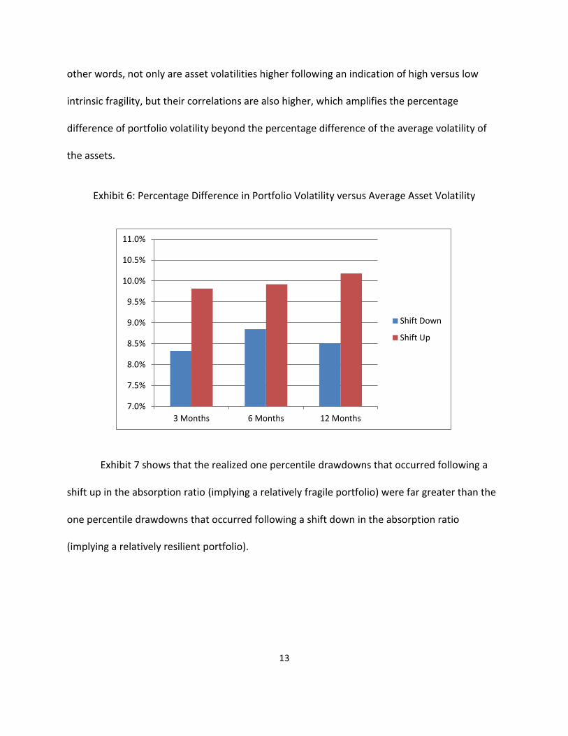
other words, not only are asset volatilities higher following an indication of high versus low
intrinsic fragility, but their correlations are also higher, which amplifies the percentage
difference of portfolio volatility beyond the percentage difference of the average volatility of
the assets.
Exhibit 6: Percentage Difference in Portfolio Volatility versus Average Asset Volatility
Exhibit 7 shows that the realized one percentile drawdowns that occurred following a
shift up in the absorption ratio (implying a relatively fragile portfolio) were far greater than the
one percentile drawdowns that occurred following a shift down in the absorption ratio
(implying a relatively resilient portfolio).
7.0%
7.5%
8.0%
8.5%
9.0%
9.5%
10.0%
10.5%
11.0%
3 Months 6 Months 12 Months
Shift Down
Shift Up

14
Exhibit 7: Subsequent 1 Percentile Realized Loss
Exhibits 5, 6, and 7 strongly suggest that the inter-temporal disparity of portfolio risk
and exposure to loss depend importantly on the portfolio’s intrinsic fragility as captured by the
absorption ratio.
One might be tempted to believe that the absorption ratio is over-engineered, that one
could obtain the same insights about portfolio fragility by measuring the average correlation of
assets. This is not so. The average correlation fails to capture the relative importance of the
assets. For example, it could be the case that assets with high volatilities experience an
increase in correlation from one period to the next, whereas assets with low volatilities
experience a decline in their correlations, such that the average correlation remains stable or
even declines. The absorption ratio, by contrast, would likely increase, given this scenario,

15
because high volatility assets are a more important determinant of portfolio risk than low
volatility assets.11
As mentioned previously, I also compute the absorption ratio based on the industries
within the U.S. equity market to capture extrinsic fragility. I focus on the U.S. equity market,
because most investors depend on their domestic equity market as the main growth engine for
their portfolios. I compute the absorption ratio of the U.S. equity market following the
calibration used by Kritzman, Li, Page, and Rigobon [2011]. They computed the absorption
based on a covariance matrix estimated from exponentially decayed daily industry returns over
a two-year window and included the 10 most important eigenvectors (top 20%) in the
numerator. This calibration is consistent with the calibration I used to compute intrinsic
fragility.
I next show how investors can employ these simple measures of intrinsic and extrinsic
fragility to reduce a portfolio’s inter-temporal risk disparity while improving its return to risk
ratio.
How to Reduce Risk Disparity
I first test a rebalancing strategy that shifts some of the portfolio’s equity exposure to Treasury
bonds following an indication of heightened intrinsic fragility. Specifically, whenever I observe
a one-standard deviation increase in intrinsic fragility, the next day I proportionately reduce the
11 Pukthuanthong, K. and R. Roll [2009] provide a formal analysis of the distinction between average correlation and their measure of market integration which they base on principal components analysis.

16
portfolio’s liquid equity positions by one half and allocate these funds to U.S. Treasury bonds.12
Exhibit 8 shows how this simple rebalancing rule affects the portfolio’s return and risk profile.
Exhibit 8: Conditioning on Intrinsic Portfolio Fragility
It is clear from Exhibit 8 that armed with information about a portfolio’s intrinsic fragility
it is possible to reduce its inter-temporal risk disparity without sacrificing its long-term growth
rate. By responding to heightened intrinsic fragility, the spread in one-year volatility falls from
19.79 percentage points to 13.65 percentage points, and the spread in three-year volatility falls
from 11.01 percentage points to 7.77 percentage points. Moreover, the portfolio’s annualized
growth rate increases slightly from 6.21% to 6.25%, and its annualized daily standard deviation
12 I base the signal on a one standard deviation move, because this calibration is consistent with the extant literature. I suspect that one could improve the strength of the signal by testing alternative thresholds, but I believe that the results are more persuasive without data mining.
0%
5%
10%
15%
20%
25%
Static Portfolio
Conditioned Portfolio
17
declines significantly from 11.13% to 8.97%, thereby improving the return to risk ratio from
0.56 to 0.70.13
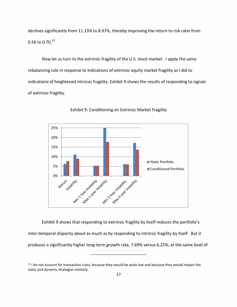
Now let us turn to the extrinsic fragility of the U.S. stock market. I apply the same
rebalancing rule in response to indications of extrinsic equity market fragility as I did to
indications of heightened intrinsic fragility. Exhibit 9 shows the results of responding to signals
of extrinsic fragility.
Exhibit 9: Conditioning on Extrinsic Market Fragility
Exhibit 9 shows that responding to extrinsic fragility by itself reduces the portfolio’s
inter-temporal disparity about as much as by responding to intrinsic fragility by itself. But it
produces a significantly higher long-term growth rate, 7.69% versus 6.25%, at the same level of
13 I do not account for transaction costs, because they would be quite low and because they would impact the static and dynamic strategies similarly.
0%
5%
10%
15%
20%
25%
Static Portfolio
Conditioned Portfolio

18
risk, 8.97%. Thus, this rebalancing strategy increases the return to risk ratio even further to
0.86. But why choose? Both signals of fragility significantly improve the return and risk profile
of the portfolio, and they are not entirely redundant. In fact, the intrinsic and extrinsic signals
are only 66% correlated. This suggests the tantalizing prospect, that in combination, they could
perform even better than they do independently, which is what I next explore.
I test a rebalancing rule that exchanges one half of the portfolio’s liquid equity exposure
for Treasury bonds, whenever there is an independent one-standard deviation spike either in
intrinsic or extrinsic fragility, and shifts the entire liquid equity position to Treasury bonds
whenever both measures of fragility spike simultaneously. The results of this rebalancing rule
are displayed in Exhibit 10.
Exhibit 10: Conditioning on Intrinsic or Extrinsic Fragility

19
Exhibit 10 shows that joint conditioning improves the portfolio’s return to risk ratio and
reduces its inter-temporal risk disparity substantially beyond what we could achieve by
independent conditioning. It produces about the same growth rate (7.61%) as extrinsic
conditioning but with a lower standard deviation a lower standard deviation (7.64%), thus
increasing the return to risk ratio from 0.56 for the static portfolio to 1.00, and it reduces both
one-year and three-year risk disparity by more than half compared to the static portfolio.
Exhibit 11 compares these metrics across all strategies.
Exhibit 11: Summary Comparison
Conditioning only on intrinsic fragility marginally increases the portfolio’s long-term
growth rate, but it significantly reduces its volatility and inter-temporal risk disparity.
Conditioning only on extrinsic fragility improves the portfolio’s long-term growth rate and one-
year risk disparity while providing about the same improvement to the portfolio’s volatility and

20
three-year risk disparity. Finally, conditioning on both intrinsic and extrinsic fragility offers
about the same improvement to long-term growth as does conditioning on extrinsic fragility,
but it substantially reduces the portfolio’s volatility and risk disparity beyond the effects of
independent conditioning.
I offer one more piece of evidence in support of the notion that conditioning on fragility
helps to distinguish relatively benign environments from relatively dangerous environments.
Exhibit 12 presents the risk premium of the policy portfolio relative to U.S. Treasury bonds for
each of these regimes.
Exhibit 12: Risk Premium of Policy Portfolio Relative to U.S. Treasury Bonds
The left bar shows the annualized risk premium of the policy portfolio relative to U.S.
Treasury bonds during periods when neither the portfolio nor the external environment
displayed evidence of fragility. These were periods during which the investor would have
-10%
-8%
-6%
-4%
-2%
0%
2%
4%
6%
Safe Intrinsic or ExtrinsicFragility
Intrinsic and ExtrinsicFragility

21
maintained the initial weights of the policy portfolio. The middle bar shows the policy
portfolio’s risk premium during periods when either the portfolio or the equity markets
exhibited evidence of fragility. During these periods the investor would have shifted half of the
portfolio’s liquid equity exposure to Treasury bonds. The right bar shows the risk premium
during periods when both the portfolio and the equity market simultaneously displayed
evidence of fragility, in which case the investor would have shifted the entire liquid equity
position to Treasury bonds. Exhibit 12 offers persuasive evidence that these measures of
fragility could help investors to capture the policy portfolio’s upside potential, while protecting
it during periods when it is especially vulnerable to losses.14
One could certainly devise more sophisticated rebalancing rules to exploit information
about intrinsic and extrinsic fragility. For example, the rules I tested respond only to signals of
heightened fragility. It may be more beneficial to scale portfolio risk symmetrically; that is, to
scale up portfolio risk following indications of resilience and to scale it down following
indications of fragility. And perhaps there are other measures that predict portfolio risk more
effectively. But it is not my purpose here to construct a sophisticated and complex rebalancing
strategy. Rather, I wish to demonstrate that merely by responding to simple and readily
observable indicators, investors can stabilize risk more effectively than by rigidly adhering to
fixed portfolio weights.
14 One might argue that any strategy that increased average exposure to bonds during this measurement period would appear favorable because bonds performed unusually well. Bonds did perform well, but as Exhibit 12 reveals, these signals of fragility effectively anticipated high risk premium, low risk premium, and negative risk premium regimes, suggesting that they should also add value during periods in which bonds perform less well.

22
The Disparity of Risk Parity
Risk disparity and the process I have proposed for addressing this problem apply not only to
policy portfolios but to any risky strategy that maintains relatively fixed weights, including the
popular strategy called risk parity. This strategy proposes that investors construct portfolios so
that each of its assets contributes equally to total portfolio risk. This strategy requires investors
to lever up the risk of relatively low risk assets and to reduce exposure to relatively high risk
assets. It is designed to impose cross-sectional risk parity within the portfolio. But even if a
portfolio derives its risk equally from the components within it, the portfolio will still experience
significant disparity in its risk through time. The strategy that I have described is designed to
mitigate inter-temporal disparity in risk, and it can be applied to risk parity strategies as well as
to policy portfolios. Investors who seek cross-sectional risk parity could maintain risk parity
across assets by uniformly scaling up and down risk within the portfolio for the purpose of
reducing inter-temporal disparity of total portfolio risk. Investors do not have to choose
between cross-sectional risk parity and inter-temporal risk parity.
Conclusion
Peter Bernstein posed a formidable challenge to the time-honored practice of establishing a
policy portfolio for the purpose of expressing an investor’s return and risk preferences. He
correctly pointed out that a portfolio’s risk profile is not constant through time, and he
therefore argued that investors manage their portfolios more opportunistically.

23
I document the inter-temporal disparity of portfolio risk, and I propose that investors
replace rigid policy portfolios with flexible investment policies. Specifically, I describe how to
measure intrinsic portfolio fragility, and I show how a simple rebalancing rule helps to mitigate
the inter-temporal disparity of portfolio volatility while at the same time improving the
portfolio’s return to risk ratio. In addition, I measure the extrinsic fragility of the equity market,
and I show how it too can be used to scale portfolio risk advantageously. Finally, I combine
signals of both intrinsic and extrinsic fragility, showing that in combination, they perform even
better than either one does independently. I argue that by monitoring both intrinsic and
extrinsic fragility investors may be able to institute a flexible investment policy that produces a
substantially more stable risk profile than a policy portfolio that adheres rigidly to a fixed set of
asset weights.

24
References
Bernstein, P., “Are Policy Portfolios Obsolete, and If So, Why?” Phoenix, AZ, January, 2003. Bernstein, P., “Back to the Future: The Policy Portfolio Revisited,” Commonfund Endowment Institute, New Haven, CT, July 10, 2007. Cremers, J.H., M. Kritzman, and S. Page, “Optimal Hedge Fund Allocation: Do Higher Moments Matter?” The Journal of Portfolio Management, Spring 2005. Karlin, S. and H. Taylor, A First course in Stochastic Processes (2nd ed.) (New York: Academic Press, 1975). Kinlaw, W, M. Kritzman, and D. Turkington, “Toward Determining Systemic Importance,” The Journal of Portfolio Management, Summer 2012.
Kritzman, M., Y. Li, S. Page, and R. Rigobon, “Principal Components as a Measure of Systemic Risk,” The Journal of Portfolio Management, Summer 2011.
Office of Financial Research Annual Report 2012, United States Treasury Department, page 43. Pukthaunthong, K. and R. Roll, “Global Market Integration: An Alternative Measure and Its Application,” Journal of Financial Economics, 94 (2009).
Samuelson, Paul A., “Summing Up on Business Cycles: Opening Address,” in Jeffrey C. Fuhrer and Scott Schuh, Beyond Shocks: What Causes Business Cycles, Boston: Federal Reserve Bank of Boston, 1998.