MIT OpenCourseWare Haus, Hermann A., and James R. …€¦ · · 2017-12-28Haus, Hermann A., and...

MIT OpenCourseWare httpocwmitedu

Haus Hermann A and James R Melcher Solutions Manual for Electromagnetic Fields and Energy (Massachusetts Institute of Technology MIT OpenCourseWare) httpocwmitedu (accessed MM DD YYYY) License Creative Commons Attribution-NonCommercial-Share Alike Also available from Prentice-Hall Englewood Cliffs NJ 1990 ISBN 9780132489805 For more information about citing these materials or our Terms of Use visit httpocwmiteduterms

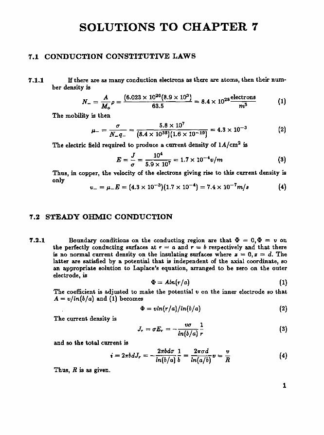
SOLUTIONS TO CHAPTER 7

71 CONDUCTION CONSTITUTIVE LAWS

T 11 H there are as many conduction electrons as there are atoms then their numshyber density is

N _ ~ _ (6023 X 1026 (89 X 103) _ 4 1028 electrons (1)- - M P - 635 - 8 X rn3 o

The mobility is then

0 58 x 107 -3 IJ- = N_q_ = (84 X 1038)(16 X 10-19) = 43 X 10 (2)

The electric field required to produce a current density of lAcm2 is

E= -J = 104

= 17 X 1O-4vrn (3) 0 59 X 107

Thus in copper the velocity of the electrons giving rise to this current density is only

(4)

72 STEADY OHMIC CONDUCTION

T 21 Boundary conditions on the conducting region are that Clgt = 0 Clgt = v on the perfectly conducting surfaces at r = a and r = b respectively and that there is no normal current density on the insulating surfaces where z = 0 z = d The latter are satisfied by a potential that is independent of the axial coordinate so an appropriate solution to Laplaces equation arranged to be zero on the outer electrode is

Clgt = Aln(r a) (1) The coefficient is adjusted to make the potential v on the inner electrode so that A = vln(ba) and (1) becomes

Clgt = vln(ra)ln(ba) (2) The current density is

vO 1 (3)

In(ba) and so the total current is

211bdO 1 2110d vi = 21rbdJr = -= v=- (4)

In(ba) b In(ab) R Thus R is as given

1

7-2 Solutions to Chapter 7

122 The net current passing through the wire connected to the inner spherical electrode must be equal to the net current at any radius r

i = J da = 41rr2uE r =gt E r = 2 (1)-4Js 1rur

Thus dr ill

t = la

Erdr = -l a

- 2 = - [ - - -] (2) b 41ru b r 41ru b a

By definition 1I = iR 80 R = ltt - ~)41ru

123 (a) Associated with the uniform field is the potential

1I (p = --(y - d) (1)

d

IT the surrounding region is insulating relative to that between the elecshytrodes the normal component of the current density on the conductor surfaces bounded by the insulating surroundings is zero The potential is constrained on the remainder of the surface enclosing the conductors so the solution is uniquely specified Provided the laws are satisfied everywhere inside the conshyducting region the solution is exact The given solution does indeed satisfy the boundary conditions on the surfaces of the conducting region In the case of (a) the potential and normal component of current density must be continshyuous across the interior interface Further in the uniformly conducting regions of (a) Laplaces equation must be satisfied as it is by a uniform field In the case of (b) (724) is satisfied by the given potential

(b) The total current is related to 1I by integrating the current density over the surface of the lower conductor

(c) A similar calculation gives the resistance in the second case

cl -zdz = -UallC l (1 + -z) dz = 2ua lc = GlI (3)= Ull --1I odd 0 1 2d

124 The potential in each of the uniformly conducting regions takes the form

(1)

where the four coefficients are adjusted to make the potentials zero and 1I on the respective electrodes and make both the potential and the normal current density continuous at the interface between the conductors On the surfaces at r = a and


r = b the current density must be zero as it is for the potential of (1) because the electric field

E __ 8~ _ (Alr)i~ (2)- r 8q - (Br)l~

has no radial component Rather than proceeding to determine the four coefficients in (1) we work directly with the electric field The integration of E from one electrode to the other must be equal to the applied voltage

A B-r- + -r- = fJ (3)2 r 2 r

Further the current density must be continuous at the interface

(4)

It follows from these relations that

(5)

The current through any crosB-section of the material [say region (a)1 must be equal to that through the wire Thus

l a l a [2dOa dr]s = d OaE~dr = ( ) - fJ == GlJ (6)

b 1 + Oa Ob b r

and the resistance is2dOa ( )G = ( a) In a b (7)

1+ltAa

125 (a) From (7223)

(1)

(b) We need the electric field which follows from (7219) by using the result of (1) to evaluate Jo = iA = GfJA

(2)

Thus the unpaired charge density is evaluated using (728)

(3)


126 (a) The inhomogeneity in permittivity has no effect on the resistance It is thereshyfore given by (7225)

(b) With the steady conduction laws stipulating that the electric field is uniform the unpaired charge density follows from Gauss law

( v) v BE EaV 1pu=VmiddotEE=Vmiddot E-i =--=--------c (1)

d Y d By da (1 + ~)2

127 At a radius r the area of the conductor (and with r = a and r = b of the outer and inner electrodes respectively) is

(1)

Consistent with the insulating surfaces of the conductor is the requirement that the current density and associated electric field be radial Current conservation (fundamentally the requirement that the current density be solenoidal) then gives as a solution to the field laws

CTEr [22(1- cos i)] = i (2)

and it follows that

(3)

The voltage follows as

v = r Erdr = i(aS - 63 )611CTo(1- cos ~)6Sa (4)lb 2

and this relation takes the form i = vG where G is as given

7 28 There can be no current density normal to the interfaces of the conducting material having normals in the azimuthal direction These boundary conditions are satisfied by an axially symmetric solution in which the current density is purely radial In that case both E and J are independent of q Then the total current is related to the current density and (through Ohms law) electric field intensity at any radius r by

i = 211QdrJr = 211QdCToaEr (1) Thus

Er = 211QdCToa

(2)

and because Erdr = i(a - b) = vl a

(3)b 211QdCToa

G = 211QdaCTo(a - b) (4)

Solutions to Chapter 7 7-5

73 DISTRIBUTED CURRENT SOURCES AND ASSOCIATED FIELDS

131 In the conductor the potential distribution is a particular part comprised of the potential due to the point current soruce (6) with i p -+ I and

In order to satisfy the condition that there be no normal component of E at the interface a homogeneous solution is added that amounts to a second source of the same sign in the lower half space Of course such a current source could not really exist in the lower region so if the field in the upper region is to be given some equivalent physical situation it should be pictured as equivalent to a pair of likeshysigned point current sources in a uniform conductor In any case this second source is located at r = vz2 + (y + h)2 + z2 and hence the potential in the conductor is as given In the lower region the potential must satisfy Laplaces equation everywhere (there are no charges in the lower region) The field in this region is uniquely specified by requiring that the potential be consistent with (a) evaluated at the interface

(1)

and that it go to zero at infinity in the lower half-space The potential that matches these conditions is that of a point charge of magnitude q = 2Ieu located on the y axis at y = h the given potential

[32 (a) First what is the potential associated with a uniform line current in a uniform conductor In the steady state

(1)

and for a surface S that has radius r from the line current

KK = 27rrJr = 27rruEr =gt E r = - shy (2)

27rur

Within a constant the associated potential is therefore

K ~ = --In(r) (3)

27rU

To satisfy the requirement that there be no normal current density in the plane y = 0 the potential is that of the line current located at y = h and an image line current of the same polarity located at y = -h


Note that the normal derivative of this expression in the plane y = 0 is indeed zero

(b) In the lower region the potential must satisfy Laplaces equation everywhere and match the potential of the conductor in the plane y =o

(5)

This has the potential distribution of an image line current located at 11 = h With the magnitude of this line current adjusted so that the potential of (5) is matched at z = 0

(6)

the potential is matched at every other value of z as well

133 First the potential due to a single line current is found from the integral form of (2)

(1)

Thus for a single line current

(2)

For the pair of line currents spaced by the distance d

X X [ dCOS 4J ] Kdcos4J~ = --lln(r - dcos4J) -InrI = --In 1--- -- --------- (3)

2~q 2~q r 2~qr

74 SUPERPOSITION AND UNIQUENESS OF STEADY CONDUCTION SOLUTIONS

141 (a) At r = b there is no normal current density 80 that

(1)

while at r = a

(2)


Because the dependence of the potential must be the same as the radial derivashytive in (2) assume the solution takes the form

cos(Cb = Arcos( + B-

2shy (3)

r

Substitution into (1) and (2) then gives the pair of equations

1 -2b-~] [A] = [ 0 ] (4)[ 0 -20a S B Jo

from which it follows that

(5)

Substitution into (3) results in the given potential in the conducting region

(b) The potential inside the hollow sphere is now specified because we know that the potential on its wall is

(6)

Here the origin is included so the only potential having the required depenshydence is

Cb = Crcos( (7)

Determination of C by evaluating (7) at r = b and setting it equal to (6) gives C and hence the given interior potential What we have carried out is an inside-outside calculation of the field distribution where the inside region is outside and the outside region is inside

142 (a) This is an example of an inside-outside problem where the potential is first determined in the conducting material Because the current d~nsity normal to the outer surface is zero this potential can be determined without regard for the geometry of what may be located outside Then given the potential on the surface the outside potential is determined Given the tP dependence of the normal current density at r = b the potential in the conducting region is taken as having the form

(1)

Boundary conditions are that

8Cbb Jr = -0-- =0 (2)

8r

at r = a which requires that B = asA2 and that

(3)


at r = b This condition together with the result of (2) gives A = JoCT[(ab)3shy11 Thus the potential in the conductor is

(4)

(b) The potential in the outside region must match that given by (4) at r = a To match the 0 dependence a dipole potential is assumed and the coefficient adjusted to match (4) evaluated at r = a

a 3Joa ( )2 (5)~ = 2CT[(ab)3 _ 11 a r cos 0

143 (a) This is an inside-outside problem where the region occupied by the conductor is determined without regard for what is above the interface except that at the interface the material above is insulating The potential in the conductor must match the given potential in the plane y = -a and must have no derivative with respect to y at y = o The latter condition is satisfied by using the cosh function for the y dependence and in view of the x dependence of the potential at y = -a taking the x dependence as also being cos(Bx) The coefficient is adjusted so that the potential is then the given value at y = o

~b _ V cosh By B - cosh f3a cos x (1)

(b) in the upper region the potential must be that given by (1) in the plane y = 0 and must decay to zero as y --gt 00 Thus

~a = V cos f3x e-3Y (2)cosh f3a

144 The potential is zero at 4J = 0 and 4J = 112 so it is expanded in solutions to Laplaces equation that have multiple zeros in the 4J direction Because of the first of these conditions these are solutions of the form

~ ex rplusmnn sin nO (1)

To make the potential zero at 4J = 112

11n2 = If 21f =gt n= 24 2m m = 123 (2)

Thus the potential is assumed to take the form

2m + Bm r-2m~ = L

00

(Am r ) sin 2m4J (3) m=l


At the outer boundary there is no normal current density so

a-(r= a) =0 (4)ar

and it follows from (3) that

(5)

At r = b the potential takes the form

bull = Eco

Vm sin2mtP = V (6) m=l

The coefficients are evaluated as in (558) through (559)

Jr 2 VVn -

11 l v sin 2nOdO = - i nodd 4 0 n

Thus Am = 4vm1rb2m[l- (ab)4mJ (8)

Substitution of (8) and (5) into (8) results in the given potential

145 (a) To make the tP derivative of the potential zero at tP = 0 and tP = Q the tP dependence is made cos(n1ltPQ ) Thus solutions to Laplaces equation in the conductor take the form

where n = 0 12 To make the radial derivative zero at r = b

(2)

so that each term in the series

(8)

satisfies the boundary conditions on the first three of the four boundaries


(b) The coefficients are now determined by requiring that the potential be that given on the boundary r = a Evaluation of (3) at r = a multiplication by cos(mlrtJoe) and integration gives

a 2 a tI 1 mlrtJ tI1 mlr-- cos (-)dtJ + - cos (-tJ)dtJ2 0 oe 2 a2 oe

= fa f An [(ab) (ntra) + (ba)(ntra)]10 n=O (4)

cos (nlrtJ) cos (mlrtJ)dtJ oe oe

2oe mlr=--sm(-)

mlr 2

and it follows that (3) is the required potential with

(5)

146 To make the potential zero at tJ = 0 and tJ = Ir2 the tJ dependence is made sin(2ntJ) Then the r dependence is divided into two parts one arranged to be zero at r = a and the other to be zero at r = b

00

~ = 2 An[(ra)2n - (ar)2nJ + Bn(rb)2n - (br)2nJ sin(2ntJ) (1) n=l

Thus when this expression is evaluated on the outer and inner surfaces the boundshyary conditions respectively involve only Bn and An

~(r = a) = tla = L00

Bn[(ab)2n - (ba)2nJ sin 2ntJ (2) n=l

~(r = b) = tlb = L00

An[(ba)2n - (ab)2nJ sin2np (3) n=l

To determine the Bns (2) is multiplied by sin(2mtJ) and integrated

(4)

and it follows that for n even Bn = 0 while for n odd

(5)


A similar usage of (3) gives

(6)

By definition the mutual conductance is the total current to the outer electrode when its voltage is zero divided by the applied voltage

a I =0 = d fr

_11_1 _ ad4J = _ d fr 2

co (7)G = _- l 2 a ua l E An 4n sin 2n4Jd4J Vb Vb 0 ar r-a Vb 0 n=l a

and it follows that the mutual eonductance is

(8)

75 STEADY CURRENTS IN PIECE-WISE UNIFORM CONDUCTORS

751 To make the current density the given uniform value at infinity

Jo bull -+ --rcosOj r -+ 00 (1)

Ua

At the surface of the sphere where r = R

(2)

and (3)

In view of the 0 dependence of (I) select solutions of the form

Jo cosO

a=b

a = --rcosO + A-- b = BrcosO (4)Ua r 2

Substitution into (2) and (3) then gives

A __ JoRs (ua - Ub) bull

- Ua (2ua + Ub) (5)

and hence the given solution

---


152 These are examples of inside-outside approximations where the field in region (a) is determined first and is therefore the inside region

(a) HUbgt 0 then ~a(r =R) $lid constant =0 (1)

(b) The field must be -(Jolu)I far from the sphere and satisfy (1) at r = R Thus the field is the sum of the potential for the uniform field and a dipole field with the coefficient set to satisfy (1)

~ $lid RJo [ -r - (IR r )2] cosO (2) 0 R

(c) At r = R the normal current density is continuous and approximated by using (2) Thus the radial current density at r = R inside the sphere is

A solution to Laplaces equation having this dependence on 0 is the potential of a uniform field ~ = Brcos(O) The coefficient B follows from (3) so that

~b $lid _ 3JoR(rIR) cosO (4)Ub

In the limit where Ub gt 0 (2) and (4) agree with (a) of Prob 751

(d) In the opposite extreme where 0 gt Ub

(5)

Again the potential is the sum of that due to the uniform field that prevails at infinity and a dipole solution However this time the coefficient is adjusted so that the radial derivative is zero at r = R

$IId---RJo [ -+-r 1 ( R1 )2] (6)~ r cosO 0 R 2

To determine the field inside the sphere potential continuity is used From (6) the potential at r = R is ~b = -(3RJo2u)cos 0 and it follows that inside the sphere

b 3 RJo 1 )~ $lid ---(r R cosO (7)2 0

In the limit where 0 gt Ub (a) of Prob 751 agrees with (6) and (7)


153 (a) The given potential implies a uniform field which is certainly irrotational and solenoidal Further it satisfies the potential conditions at z = 0 and z = -I and implies that the current density normal to the top and bottom interfaces is zero The given inside potential is therefore the correct solution

(b) In the outside region above boundary conditions are that

traquo(z = Oz) = -vzj traquo(z 0) = OJ z

traquo(a z) = OJ ~(-l z) = v(1- -) (1)a

The potential must have the given linear dependence on the bottom horizontal interface and on the left vertical boundary These conditions can be met by a solution to Laplaces equation of the form sz By translating the origin of the z axis to be at z = a the solution satisfying the boundary conditions on the top and right boundaries is of the form

v traquo = A(a - z)z = - la (a - z)z (2)

where in view of (1a) and (1c) setting the coefficient A = -vl makes the potential satisfy conditions at the remaining two boundaries

(c) In the air and in the uniformly conducting slab the bulk charge density Pu must be zero At its horizontal upper interface

CTu = faE - fbE~ = -fovza (3)

Note that z lt 0 so if v gt 0 CTu gt 0 as expected intuitively The surface charge density on the lower surface of the conductor cannot be specified until the nature of the region below the plane z = -b is specified

(d) The boundary conditions on the lower inside region are homogeneous and do not depend on the outside region Therefore the solution is the same as in (a) The potential in the upper outside region is one associated with a uniform electric field that is perpendicular to the upper electrode To satisfy the condition that the tangential electric field be the same just above the interface as below and hence the same at any location on the interface this field must be uniform H it is to be uniform throughout the air-space it must be the same above the interface as in the region where the bounding conductors are parallel plates Thus

v v ()E = Ix + yl 4

The associated potential that is zero at z = 0 and indeed on the surface of the electrode where z = -zal is

v v ~ = -z+ -z (5)

a I Finally instead of (3) the surface charge density is now


154 (a) Because they are surrounded by either surfaces on which the potential is conshystrained or by insulating regions the fields within the conductors are detershymined without regard for either the fields within the square or outside where not enough information has been given to determine the fields The condishytion that there be no normal current density and hence no normal electric field intensity on the surfaces of the conductors that interface the insulating regions is automatically met by having uniform fields in the conductors Beshycause these fields are normal to the electrodes that terminate these regions the boundary conditions on these surfaces are met as well Thus regardless of what d is relative to a in the upper conductor

E = -ixj ~ = Zj J = -Oix (l) a a a

while in the conductor to the right

bull tJ tJ J tJ ( )E = -I) -j W = -1Ij = -0-1 2 a a a )

(b) In the planes 11 = a and Z = a the potential inside must be the same as given by (l) and (2) in these planes linear functions of Z and of 11 respectively It must also be zero in the phmes Z = 0 and 11 = O A simple solution meeting these conditions is

tJ ~= AZ1I= -Z1I (3)

a2

Figure Sfampbull(

(c) The distribution of potential and electric field intensity is as shown in Fig S754

155 (a) Because the potential difference between the plates either to the left or to the right is zero the electric field there must be zero and the potential that of the respective electrodes

(l)

(b) Solutions that satisfy the boundary conditions on all but the interface at z = 0 are

(2a)

Solutions to Chapter 7

DO

~b = V + L Bnenrrs4 sin n1l ya

n=1

(c) At the interface boundary conditions are

8~4 8~b-04-- = -01gt--

8z 8z

~4=~1gt

(d) The first of these requires of (2) that

Written using this the second requires that

00 DO

A n1l Oa A n1lLJ nsm-y= v- LJ - nsm-yn=1 a n=1 01gt a

7-15

(26)

(3)

(4)

(5)

(6)

The constant term can also be written as a Fourier series using an evaluationof the coefficients that is essentially the same as in (553)-(559)

DO 4v n1lv= L-sm-y

1In an=1

Thus

(Oa) 4vAn 1+- =-01gt n1l

and it follows that the required potential is

(7)

(8)

(9)

=~=I

==Ql[)~~==

Figure 57ampamp


(e) In the case where Ub gt U a the inside region is to the left where boundshyary conditions are on the potential at the upper and lower surfaces and on its normal derivative at the interface In this limit the potential is uniform throughout the region and the interface is an equipotential having ~ = tI Thus the potential in the region to the right is as shown in Fig 553 with the surface at 11 = b playing the role of the interface and the surface at 11 = 0 at infinity In the case where the region between electrodes is filled by a unishyform conductor the potential and field distribution are as sketched in Fig 8755 In the vicinity of the regions where the electrodes abut the potential becomes that illustrated in Fig 572 By symmetry the plane z = 0 is one having the potential ~ = tI2

(f) The surface at 11 = a2 is a plane of symmetry in the previous configuration and hence one where E = O Thus the previous solution applies directly to finding the solution in the conducting layer

76 CONDUCTION ANALOGS

161 The analogous laws are

E=-V~ E=-V~ (1)

VUE=8 VEE=pu (2)

The systems are normalized to different length scales The conductivity and pershymittivity are respectively normalized to U c and Epound respectively and similarly the potentials are normalized to the respective voltages Vc and Vpound

(z 11 z) = (~ll amp)lpound (3)

~=Vc~ ~=Vpound~ (4)

E = (Vclc)~ E = (Vpoundlpound)~ (5)

8 = (ucVc~)I (6)

Pu = (EpoundVdl~)p (7)-U

By definition the normalized quantities are the same in the two systems

Q(r) = euro(r) (8)

I(r) = u(r) (9)

so that both systems are represented by the same normalized laws

E=-~ (10)


(11) Thus the capacitance and conductance are respectively

C = fEIEpoundfE d1 LE d (12)

G = uele poundd dll Lampmiddot dll (13)

where again by definition the normalized integral ratios in (12) and (13) are the same number Thus

~G=~~=~ (~ U e Ie U Ie

Note that the deductions summarized by (763) could be made following the same normalization approach

77 CHARGE RELAXATION IN UNIFORM CONDUCTORS

111 (a) The charge is given when t = 0

1r1r ()P = Pi sm ~ xsm 1

Given the charge density none of the bulk or surface conditions needed to determine the field involve time rates of change Thus the initial potential distribution is determined from the initial conditions alone

(b) The properties of the region are uniform so (3) and hence (4) apply directly Given the charge is (c) of Prob 414 when t = 0 the subsequent distribution of charge is

bull 1r bull 1r tff f (2)P = Po ()t sm ~zsm bY Po = Pie- j T ==

(c) As in (a) at each instant the charge density is known and all other conditions are independent of time rates of change Thus the potential and field distrishybutions simply go along with the changing charge density They follow from (a) and (b) of Prob 414 with Po(t) given by (2)

(d) Again with Po(t) given by (2) the current is given by (6) of Prob 414

112 (a) The line charge is pictured as existing in the same uniformly conducting mashyterial as occupies the surrounding region Thus (773) provides the solution

AI = AI(t = O)e-tff T = fu (1)

(b) There is no initial charge density in the surrounding region Thus the charge density there is zero

(c) The potential is given by (1) of Probe 454 with AI given by (1)


113 (a) With q lt -qc the entire surface of the particle can collect the ions Equation (7710) becomes simply

i = -pp61fR2 E a r (cos6 +) sin6d6 (1)Jo qc

Integration and the definition of qc results in the given current

(b) The current found in (a) is equal to the rate at which the charge on the particle is increasing

dq pp -=--q (2)dt E

This expression can either be formally integrated or recognized to have an exponential solution In either case with q(t = 0) = qo

(3)

114 The potential is given by (5913) with q replaced by qc as defined with (7711)

~ = -EaRcos6[ _ (Rr)2] + 121rEoR2Ea (1)R 41rEo r

The reference potential as r - 00 with 6 = 1f2 is zero Evaluation of (1) at r = R therefore gives the particle potential relative to infinity in the plane 6 = 1r2

~= 3REa (2)

The particle charges until it reaches 3 times a potential equal to the radius of the particle multiplied by the ambient field

78 ELECTROQUASISTATIC CONDUCTION LAWS FOR INHOMOGENEOUS MATERIAL

181 For t lt 0 steady conduction prevails so a( )at = 0 and the field distribushytion is defined by (741)

v middot(uV~) =-8 (1)

where ~ = ~I on Sj -uV~ = 3I on S (2)

To see that the solution to (1) subject to the boundary conditions of (2) is unique propose different solutions ~a and ~b and define the difference between these solushytions as

~d = ~a - ~b (3)


Then it follows from (1) and (2) that

(4)

where ~d = 0 on S (5)

Multiplication of (4) by ~d and integration over the volume V of interest gives

Gauss theorem converts this expression to

(7)

The surface integral can be broken into one on S where ~d = 0 and one on SIt where UV~d = O Thus what is on the left in (7) is zero If the integrand of what is on the right were finite anywhere the integral could not be zero so we conclude that to within a constant ~d = 0 and the steady solution is unique

For 0 lt t the steps beginning with (7811) and leading to (7815) apply Again the surface integration of (7811) can be broken into two parts one on S where ~d = 0 and one on SIt where -UV~d = O Thus (7816) and its implications for the uniqueness of the solution apply here as well

19 CHARGE RELAXATION IN UNIFORM AND PIECEshyWISE UNIFORM SYSTEMS

T91 (a) In the first configuration the electric field is postulated to be uniform throughshyout the gap and therefore the same as though the lossy segment were not present

E = irvrln(ab) (1)

This field is iITotational and solenoidal and integrates to v between r = b and r = a Note that the boundary conditions at the interfaces between the lossy-dielectric and the free space region are automatically met The tangential electric field (and hence the potential) is indeed continuous and because there is no normal component of the electric field at these interfaces (7912) is satisfied as well

(b) In the second configuration the field is assumed to take the piece wise form

Rltrlta (2)b lt r lt R


where A and B are determined by the requirements that the applied voltage be consistent with the integration of E between the electrodes and that (7912) be satisfied at the interface

Aln(aR) + bln(Rb) = 4) (3)

w [EoA _ Ebb] _ ub = 0 (4)R R R

It follows that A = (WEb + u)vDet (5)

J =wEovDet (6)

where Det is as given and the relations that result from substitution of these coefficients into (2) are those given

(c) In the first case the net current to the inner electrode is

l bull 1[( )b b I v lobuv =1w 271 - 0 Eo + 0 E bln(ab) + bln(ab) (7)

This expression takes the form of the impedance of a resistor in parallel with a capacitor where

i = vG + jwCv (8)

Thus the C and G are as given in the problem In the second case the equivalent circuit is given by Fig 795 which implies

that l v(wCa )(1 + wRCb)= (9)

1 + jwR(Ca + Cb)

In this case the current to the inner electrode follows from (6) as

27ll~middotWE(1 + i)l In a R tT = ---_gt~-------~ (10)

1 + jwln(Rlb) [~ + E ] tT InlalR) n(rlb)

Comparison of these last two expressions results in the given parameters

192 (a) In the first case where the interface between materials is conical the electric field intensity is what it would be in the absence of the material

(1)

This field is perpendicular to the perfectly conducting electrodes has a continshyuous tangential component at the interface and trivially satisfies the condition of charge conservation at the interface


In the second case where the interface between materials is spherical the field takes the form

E _ R 1-2j R lt r lt a -I e A (2)

Dr2j bltrltR

The coefficients are adjusted to satisfy the condition that the integral of E from r = b to r = a be equal to the voltage

11 111 A(---)+D(---)=v (3)R a b R

and conservation of charge at the interface (7912)

0 A bull (1 ~) 0--D+3W f --f- == (4)R2 Ow W

Simultaneous solution of these expressions gives

1 = (0 + jWf)fJDet (5)

iJ = jWfoDet

wherea-R [a-R R-b]

Det= O(~) + 3W f(~) + fo(---Il)

which together with (2) give the required field

(b) In the first case the inner electrode area subtended by the conical region ocshycupied by the material is 271b2 [1- cos(a2)J With the voltage represented as v = Re fJexp(jwt) the current from the inner spherical electrode which has the potential v is

(6)

Equation (6) takes the same form as for the terminal variables of the circuit shown in Fig S792a Thus

(7)

abO G = 271[1 - cos(a2)Jshy

a- b

(271-a)]abfoCa = 271 [1 - cos -2- a _ b (8)


abfCb = 211[1 - cos(a2)] a _ b

t-+v

(a)

t-bull+

v

(b)

Flpre Sf9J

(9)

(11)

(12)

(10)= 411Rba _ w(411RbE + 411aR Eg )R-b R-b a-R

This takes the same form as the relationship between the terminal voltageand current for the circuit shown in Fig S792b

I wCa(G + wCb) ~t= v

G + w(Ca + Cb)Thus the elements in the equivalent circuit are

G = 4 Rbu C = 41rRbfo bull Cb

= 41rRbf1r R _ b a R-b I R-b

In the second case the current from the inner electrode is

I 2(ufJ fJ)t = 41rb b2 + wfb2

w( 411aREg ) (4l1Rba + w 411Rb f)a-R R-b R-b

793 In terms of the potential v of the electrode the potential distribution andhence field distribution are

(3)

(2)

(1)va

~ = v(ar) =gt E = il2r

The total current into the electrode is then equal to the sum of the rate of increaseof the surface charge density on the interface between the electrode and the mediaand the conduction current from the electrode into the media

i = l [t fEr +uEr]da

In view of (1) this expression becomes

(fa dv ua) dvt = 21ra2

- - + -v = 21rfa- + (21rua)va2 dt a2 dt

The equivalent parameters are deduced by comparing this expression to one deshyscribing the current through a parallel capacitance and resistance


J 194 (a) With A and B functions of time the potential is assumed to have the same

dependence as the applied field

cos ~a = -Ercos+A-shy(1)

r

~b = Brcos (2)

The coefficients are determined by continuity of potential at r = a

(3)

and the combination of charge conservation and Gauss continuity condition alsoatr=a

(UaE - ubE~) + t(faE - fbE~) = 0 (4)

Substitution of (1) and (2) into (3) and (4) gives

A A - - Ba = Ea =gt B = - - E (5)a a2

A d A CTa(E - a2) + Ub B + dt [fa(E + a2) + fb B ] = 0 (6)

and from these relations

With Eo the magnitude of a step in E(t) integration of (7) from t = 0- when A = 0 to t = 0+ shows that

(8)

A particular solution to (7) for t gt 0 is

A = (Ub - ua)a2Eo (9)Ub+Ua

while a homogeneous solution is exp(-tT) where

(10)

Thus the required solution takes the form


where the coefficient Al is determined by the initial condition (8) Thus

[(fb- fa) (Ub - Ua )] 2E -t + (Ub - Ua ) 2EA --(fb + fa)

-(Ub + Oa)

a oe (Ub + u a )

a 0 (12)

The coefficient B follows from (5)

AB= --Eo (13)

a2

In view of this last relation and then (12) the unpaired surface charge density is

A A U au = fa (Eo + R2) + fb( R2 - Eo)

(14) = 2(faUb - fbUa) E (1 _ e- t )

Ua + Ub o

(b) In the sinusoidal steady state the drive in (7) takes the form Re texp(jwt) and the resonse is of the form Re 4exp(jwt) Thus (7) shows that

4 - [(Ub - u a ) + jW(fb - fall 2 t (15) - (Ob + u a ) + jW(fb + fa) a p

and in turn from (5)

lJ = _ 2(ua + jWfa ) (16) (Ub + u a ) + jW(fb + fa)

This expressions can then be used to show that the complex amplitude of the unpaired surface charge density is

A 2(Ubfa - Uafb) ( )

U au = (Ub + Ua ) + jW(fb + fa) 17

(c) From (1) and (2) it is clear that the plane ltp = 7f2 is one of zero potential regardless of the values of the drive E(t) or of A or B Thus the z = 0 plane can be replaced by a perfect conductor In the limit where U a --+ 0 and W(fa + fb)Ub lt 1 (15) and (16) become

(18)

iJ --+ - 2jwfa E (19) Ub p

Substitution of these coefficients into the sinusoidal steady state versions of (1) and (2) gives

~a = -Re EA a [r- - -a] cosltpeJw t (20)Par

A b R 2jwfa E Jmiddotwt =-e--pe (21) Ub

These are the potentials that would be obtained under sinusoidal steady state conditions using (a) and (b) of Prob 795


195 (a) This is an example of an inside-outside situation The inside region is the one where the excitation is applied namely region (a) In so far as the field in the exterior region is concerned the surface is essentially an equipotential Thus the solution given by (a) must be constant at r = a (it is zero) must become the uniform applied field at infinity (which it does) and must be comprised of solutions to Laplaces equation (which certainly the uniform and dipole fields are)

(b) To approximate the interior field note that in general charge conservation and Gauss law (7912) require that

(1)

So long as the interior field is much less than that applied this expression can be approximated by

(2)

which in view of (a) is a prescription for the normal conduction current denshysity inside the cylinder This is then the boundary condition on the potential in region (b) the interior of the cylinder and it follows that the potential within is

b 2fo dE Clgt = Arcosq = --rcosqdt (3)

Note that the approximation made in going from (1) to (2) is valid if

f dEfo~gt f~ ~ f02cosOEgt -f02cosq-d (4)

0 t

Thus if E(t) = Eocoswt the approximation is valid provided

1 gtshyWf (5) U

V 196 (a) Just after the step there has been no time for the relaxation of unpaired

charge so the system is still behaving as if the conductivity were zero In any case piece-wise solutions to Laplaces equation having the same 0 dependence as the dipole potential and having the dipole potential in the neighborhood of the origin are

(1)

b P cosOClgt = ---- + Br cos 0 (2)

411fo r 2

At r = a Clgta = Clgtb (3)


a~a a~b -f--=-f - (4)ar 0 ar

Substitution of (1) and (2) into these relations gives

[ -s- -a] [A] P [a] (5)t fo B = 411foa3 1

Thus the desired potentials are (1) and (2) evaluated using A and B found from (5) to be

A= ~ (6)411(fo + 2f)

B = 2(fo - f)p ( ) 411foa3(fo + 2f) 7

(b) After a long time charge relaxes to the interface to render it an equipotential Thus the field outside is zero and that inside is determined by making Bin (2) satisfy the condition that ~b(r = a) = O

A=O (8)

B=--Pshy (9)411foa3

(c) In the general case (4) is replaced by

a~a a a~a a~b

ua- + at (fa- - fo ar ) = 0 (10)

and substitution of (1) and (2) gives

2uA + dd [2fA + fo( -2p + B(3 )] = 0 (11)t 411fo

With B replaced using (5a)

dA A 3 dp 2f+fo-+-- T=-shy (12)dt T - 411(2f + fo) dt 2u

With p a step function integration of this expression from t = 0- to t = 0+ gives

(13)

It follows that

(14)

and in tum that T

Po 1 ) (3e- t

B = 411a3 2f + f - f (15)o o

As t - 0 these expressions become (6) and (7) while as t - 00 they are consistent with (8) and (9)


191 (a) This is an fIIinside-outside- situation where the layer of conductor is the fIIin_ side- region The potential is constrained at the lower surface by the electrodes and the y derivative of the potential must be zero at the upper surface This potential follows as

ebb - V cosh fjy Q (1) - cosh fjd cos 1JZ

The potential must be continuous at the upper interface where it follows from (1) with y = 0 that it is

ebG(y = 0) = V cos fjz (2)coshfjd

The potential that matches this condition in the plane y = 0 and goes to zero as y goes to infinity is

ebG= V cosfjz e-J (3) coshfjd

Thus before t = 0 the surface charge density is

ebG ebb a u = - [euroo aa _ euro aa ] = euroofjV cosfjz (4)

y y 1=0 cosh fjd

(b) Once the potential imposed by the lower electrodes is zero the potentials in the respective regions take the form

ebG= Ae-JI cos fjz (Sa)

b _ Asinhfj(y + d) Q (Sb) I - sinhfjd cos1Jz

Here the coefficients have been adjusted so that the potential is continuous at y = o The remaining condition to be satisfied at this interface is (7912)

b) bata (eurooE - euroE - aE = 0 (6)

Substitution from (S) shows that

ata [(euroofj + eurocothfjd) cos ltp A]+ afj cothfjdcos ltpA = 0 (7)

The term inside the time derivative is the surface charge density Thus (7) can be converted to a differential equation for the surface charge density

dt1a aa dt+~=O (8)

where T= ( eurootanhfjd+euro)a

Thus given the initial condition from part (a) the surface charge density is

_ euroofjV cos fjz -tIT (9) aa - cosh fjd e


198 (a) Just after Qhas been turned on there is still no surface charge on the interface Thus when t = 0+

~ltI(y = 0) = ~b(y = 0) (1)

B~ltI B~b Eo-(Y = 0) = E-(Y = 0) (2)

By By

It follows from the postulated solutions that

(3)

-EoQ - Eoqb = -Eqltl (4)

and finally that qltl(O+) and qb(O+) have the given values

(b) As t -+ 00 the interface becomes an equipotential It follows from the postushylated solution evaluated at the interface where the potential must be what it is at infinity namely zero that

(5)

(c) Throughout the transient (1) must hold However the condition of (2) is generalized to represent the buildup ofthe surface charge density (7912) At y=O

(6)

When t gt 0 Q is a constant Thus evaluation of (6) with the postulated solutions gives

dqb dqltlE0-U - Edt - uqltl = 0 (7)

Using (1) to eliminate qb this expression becomes

(8)

where T = (Eo + E)U The solution to this expression is Aexp(-tT) where A is the initial value found in part (a) The other image charge qb is then given by using (1)

199 (a) As t -+ 00 the surface at z = 0 requires that there be no normal current density and hence electric field intensity on the (b) side Thus all boundary conditions in region (b) and Laplaces equation are satisfied in region (b) by a uniform electric field and a linear potential

(1)


The field in region (a) can then be found It has a potential that is zero on three of the four boundaries On the fourth where z = 0 the potential must be the same as given by (1)

(2)

To match these boundary conditions we take the solution to Laplaces equashytion to be an infinite sum of modes that satisfy the first three boundary conditions

~ = _ ~ An sinh ~(z - b) sin (nllY) (3) LJ sinh (mrb) a n=l

The coefficients are determined by requiring that this sum satisfy the last boundary condition at z = o

co

v = LAnsm-)(nllY (4)-(a - y)a a

n=l

Multiplication by sin(mllya) and integration from z = 0 to z = a gives

21 v mllY) 2vAm = - -(a- y)sm(- dy=- (5)a 0 a a mll

Thus it follows that the potential in region (a) is

(6)

(b) During the transient the two regions are coupled by the temporal and spatial evoluation of unpaired charge at the interface where z = o So in region (b) we add to the asymptotic solution which satisfies the conditions on the potential at y = 0 y = a and as z -+ -00 one that term-by-term is zero on these boundaries and as z -+ -00 and that term-by-term satisfies Laplaces equation

co b v nlly~ = -(a - y) + LJ Bn en 1l sm (-) (7)

a n=l a

The result of (4)-(5) shows that the first term on the right can just as well be represented by the same Fourier series for its y dependence as the last term

Ab ~ 2v (nllY) ~ B n1l bull (nllY)It = LJ - sm -- + LJ n e sm-- (8)

n=l nll a n=l a

The potential in region (a) can generally take the form of (3) There remains finding An(t) and Bn(t) such that the continuity conditions at z = 0 on the potential and representing Gauss plus charge conservation are met Evaluation


of (3) and (8) at z = 0 shows that the potential continuity condition can be satisfied term-by-term if

2vA = -+B (9)

n1l

The second condition brings in the dynamics (7912) at z = 0

(10)

Substitution from (3) and (8) gives an expression that can also be satisfied term-by-term if

n1l (n1lb) n1l n1l (n1lb dA-ua - coth - A - ub-B - Ea - coth -)- shya a a a a dt (11)

n1ldB-Eb---=O

b dt

Substitution for B from (9) then gives one expression that describes the temporal evolution of A(t)

(12)

whereE coth (1lb) + E

T = a a b

- Ua coth (nb) + Ub

To find the response to a step the volue of A when t o is found by integrating (12) from t = 0- when A = 0 to t = 0+

(13)

The solution to (12) which takes the form of a homogeneous solution exp(-tIT) and a constant particular solution must then satisfy this initial condition

A = A1 e -tiT + Ub

(-2 )

( Vob) (14)

n1l Ua coth + Ub

The coefficient of the homogeneous term is adjusted to satisfy (13) and (14) becomes

(15)


There is some insight gained by writing this expression in the alternative form

Given this expression for An Bn follows from (9) In this specific situation these expressions are satisfied with U a = 0 and Ea = Eo

(c) In this limit it follows from (15) that as t - 00 An - Vo2nll) and this is consistent with what was found for this limit in part (a) (5)

With the permittivities equal the potential and field distributions just after the potential has been turned on and therefore as there has been no time for unpaired charge to accumulate at the interface is as shown in Fig 8799a To make this sketch note that far to the left the equipotentials are equally spaced straight lines (surfaces) running parallel to the boundaries which are themselves equipotentials All of these must terminate in the gap at the origin In the neighborhood of that gap the potential has the form familiar from Fig 572 (except that the equipotential =V is at tP = II and not at tP = 211-)

(a)

(b)

Figure Sf99

In the limit where t - 00 the uniform equipotentials in region (b) extend up to the interface Just as we could solve for the field in region (b) and then for that in region (a) we can also draw the fields iIi th~t order In region (a) the potential is linear in y in the plane z = 0 and zero on the other two boundaries Thus the equipotentials that originate on the boundary at


z = 0 at equal distances must terminate in the gap where they converge like equally spaced spokes on the hub of a wheel

The transient that we have described takes the field distribution from that of Fig 8799a where there is a conduction current normal to the interface from the (b) region side supplying surface charge to the interface to that of Fig S799b where the current density normal to the surface has subsided because charges on the interface have created just that field necessary to null the normal field in region (b)

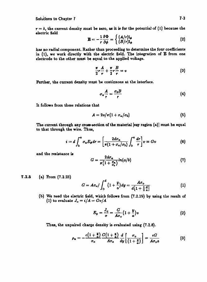
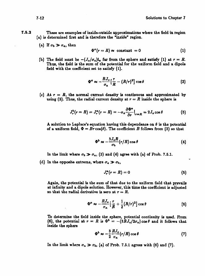
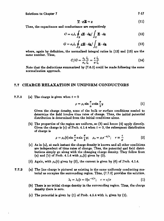
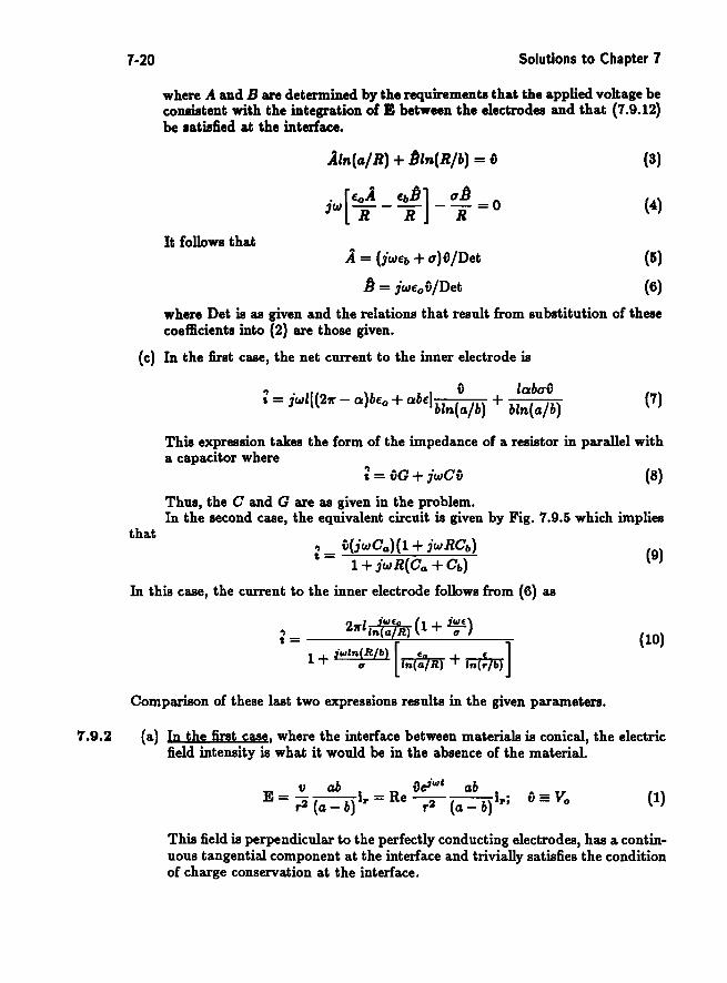
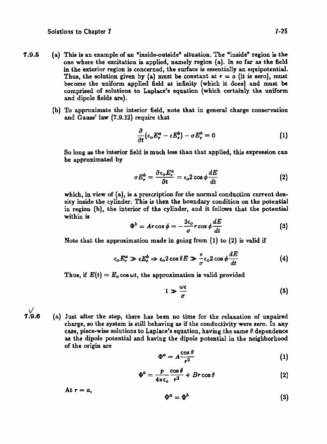
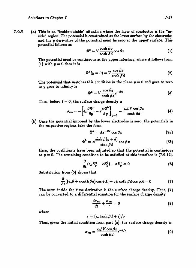
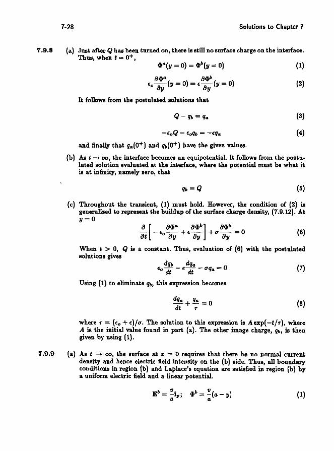SOLUTIONS TO CHAPTER 7

71 CONDUCTION CONSTITUTIVE LAWS

T 11 H there are as many conduction electrons as there are atoms then their numshyber density is

N _ ~ _ (6023 X 1026 (89 X 103) _ 4 1028 electrons (1)- - M P - 635 - 8 X rn3 o

The mobility is then

0 58 x 107 -3 IJ- = N_q_ = (84 X 1038)(16 X 10-19) = 43 X 10 (2)

The electric field required to produce a current density of lAcm2 is

E= -J = 104

= 17 X 1O-4vrn (3) 0 59 X 107

Thus in copper the velocity of the electrons giving rise to this current density is only

(4)

72 STEADY OHMIC CONDUCTION

T 21 Boundary conditions on the conducting region are that Clgt = 0 Clgt = v on the perfectly conducting surfaces at r = a and r = b respectively and that there is no normal current density on the insulating surfaces where z = 0 z = d The latter are satisfied by a potential that is independent of the axial coordinate so an appropriate solution to Laplaces equation arranged to be zero on the outer electrode is

Clgt = Aln(r a) (1) The coefficient is adjusted to make the potential v on the inner electrode so that A = vln(ba) and (1) becomes

Clgt = vln(ra)ln(ba) (2) The current density is

vO 1 (3)

In(ba) and so the total current is

211bdO 1 2110d vi = 21rbdJr = -= v=- (4)

In(ba) b In(ab) R Thus R is as given

1




Thus dr ill

t = la

Erdr = -l a

- 2 = - [ - - -] (2) b 41ru b r 41ru b a



1I (p = --(y - d) (1)

d






(1)




E __ 8~ _ (Alr)i~ (2)- r 8q - (Br)l~


A B-r- + -r- = fJ (3)2 r 2 r


(4)


(5)



b 1 + Oa Ob b r


1+ltAa

125 (a) From (7223)

(1)


(2)


(3)





d Y d By da (1 + ~)2


(1)


CTEr [22(1- cos i)] = i (2)

and it follows that

(3)






Er = 211QdCToa

(2)


(3)b 211QdCToa

G = 211QdaCTo(a - b) (4)





(1)



(1)



27rur


K ~ = --In(r) (3)

27rU





(5)


(6)



(1)


(2)



2~q 2~q r 2~qr



(1)

while at r = a

(2)




2shy (3)

r


1 -2b-~] [A] = [ 0 ] (4)[ 0 -20a S B Jo


(5)



(6)


Cb = Crcos( (7)



(1)


8Cbb Jr = -0-- =0 (2)

8r


(3)



(4)


a 3Joa ( )2 (5)~ = 2CT[(ab)3 _ 11 a r cos 0








11n2 = If 21f =gt n= 24 2m m = 123 (2)


2m + Bm r-2m~ = L

00




a-(r= a) =0 (4)ar


(5)


bull = Eco



Jr 2 VVn -






(2)


(8)







2oe mlr=--sm(-)

mlr 2


(5)


00



~(r = a) = tla = L00


~(r = b) = tlb = L00



(4)


(5)



(6)


a I =0 = d fr

_11_1 _ ad4J = _ d fr 2



(8)




Ua


(2)

and (3)


Jo cosO

a=b




- Ua (2ua + Ub) (5)


---











(5)


$IId---RJo [ -+-r 1 ( R1 )2] (6)~ r cosO 0 R 2


b 3 RJo 1 )~ $lid ---(r R cosO (7)2 0






traquo(a z) = OJ ~(-l z) = v(1- -) (1)a








v v ()E = Ix + yl 4


v v ~ = -z+ -z (5)








tJ ~= AZ1I= -Z1I (3)

a2

Figure Sfampbull(



(l)


(2a)


DO


n=1


8~4 8~b-04-- = -01gt--

8z 8z

~4=~1gt



00 DO


7-15

(26)

(3)

(4)

(5)

(6)


DO 4v n1lv= L-sm-y

1In an=1

Thus

(Oa) 4vAn 1+- =-01gt n1l


(7)

(8)

(9)

=~=I

==Ql[)~~==

Figure 57ampamp






E=-V~ E=-V~ (1)

VUE=8 VEE=pu (2)



~=Vc~ ~=Vpound~ (4)


8 = (ucVc~)I (6)



Q(r) = euro(r) (8)

I(r) = u(r) (9)


E=-~ (10)






~G=~~=~ (~ U e Ie U Ie



















dq pp -=--q (2)dt E


(3)




~= 3REa (2)







~d = ~a - ~b (3)



(4)




(7)





E = irvrln(ab) (1)






Aln(aR) + bln(Rb) = 4) (3)

w [EoA _ Ebb] _ ub = 0 (4)R R R


J =wEovDet (6)





i = vG + jwCv (8)



1 + jwR(Ca + Cb)






(1)




E _ R 1-2j R lt r lt a -I e A (2)

Dr2j bltrltR


11 111 A(---)+D(---)=v (3)R a b R


0 A bull (1 ~) 0--D+3W f --f- == (4)R2 Ow W


1 = (0 + jWf)fJDet (5)

iJ = jWfoDet

wherea-R [a-R R-b]

Det= O(~) + 3W f(~) + fo(---Il)



(6)


(7)


a- b

(271-a)]abfoCa = 271 [1 - cos -2- a _ b (8)


abfCb = 211[1 - cos(a2)] a _ b

t-+v

(a)

t-bull+

v

(b)

Flpre Sf9J

(9)

(11)

(12)











(3)

(2)

(1)va






- - + -v = 21rfa- + (21rua)va2 dt a2 dt






r

~b = Brcos (2)


(3)


(UaE - ubE~) + t(faE - fbE~) = 0 (4)


A A - - Ba = Ea =gt B = - - E (5)a a2




(8)




(10)





-(Ub + Oa)

a oe (Ub + u a )

a 0 (12)


AB= --Eo (13)

a2



(14) = 2(faUb - fbUa) E (1 _ e- t )

Ua + Ub o







U au = (Ub + Ua ) + jW(fb + fa) 17


(18)

iJ --+ - 2jwfa E (19) Ub p








(1)


(2)





0 t


1 gtshyWf (5) U



(1)


411fo r 2



a~a a~b -f--=-f - (4)ar 0 ar


[ -s- -a] [A] P [a] (5)t fo B = 411foa3 1


A= ~ (6)411(fo + 2f)

B = 2(fo - f)p ( ) 411foa3(fo + 2f) 7


A=O (8)

B=--Pshy (9)411foa3


a~a a a~a a~b

ua- + at (fa- - fo ar ) = 0 (10)


2uA + dd [2fA + fo( -2p + B(3 )] = 0 (11)t 411fo




(13)

It follows that

(14)

and in tum that T

Po 1 ) (3e- t

B = 411a3 2f + f - f (15)o o











y y 1=0 cosh fjd









dt1a aa dt+~=O (8)






~ltI(y = 0) = ~b(y = 0) (1)

B~ltI B~b Eo-(Y = 0) = E-(Y = 0) (2)

By By


(3)




(5)


(6)




(8)



(1)



(2)




co


n=l




(6)



a n=l a



n=l nll a n=l a




2vA = -+B (9)

n1l


(10)



n1ldB-Eb---=O

b dt


(12)


T = a a b

- Ua coth (nb) + Ub


(13)


A = A1 e -tiT + Ub

(-2 )

( Vob) (14)

n1l Ua coth + Ub


(15)






(a)

(b)

Figure Sf99








Thus dr ill

t = la

Erdr = -l a

- 2 = - [ - - -] (2) b 41ru b r 41ru b a



1I (p = --(y - d) (1)

d






(1)




E __ 8~ _ (Alr)i~ (2)- r 8q - (Br)l~


A B-r- + -r- = fJ (3)2 r 2 r


(4)


(5)



b 1 + Oa Ob b r


1+ltAa

125 (a) From (7223)

(1)


(2)


(3)





d Y d By da (1 + ~)2


(1)


CTEr [22(1- cos i)] = i (2)

and it follows that

(3)






Er = 211QdCToa

(2)


(3)b 211QdCToa

G = 211QdaCTo(a - b) (4)





(1)



(1)



27rur


K ~ = --In(r) (3)

27rU





(5)


(6)



(1)


(2)



2~q 2~q r 2~qr



(1)

while at r = a

(2)




2shy (3)

r


1 -2b-~] [A] = [ 0 ] (4)[ 0 -20a S B Jo


(5)



(6)


Cb = Crcos( (7)



(1)


8Cbb Jr = -0-- =0 (2)

8r


(3)



(4)


a 3Joa ( )2 (5)~ = 2CT[(ab)3 _ 11 a r cos 0








11n2 = If 21f =gt n= 24 2m m = 123 (2)


2m + Bm r-2m~ = L

00




a-(r= a) =0 (4)ar


(5)


bull = Eco



Jr 2 VVn -






(2)


(8)







2oe mlr=--sm(-)

mlr 2


(5)


00



~(r = a) = tla = L00


~(r = b) = tlb = L00



(4)


(5)



(6)


a I =0 = d fr

_11_1 _ ad4J = _ d fr 2



(8)




Ua


(2)

and (3)


Jo cosO

a=b




- Ua (2ua + Ub) (5)


---











(5)


$IId---RJo [ -+-r 1 ( R1 )2] (6)~ r cosO 0 R 2


b 3 RJo 1 )~ $lid ---(r R cosO (7)2 0






traquo(a z) = OJ ~(-l z) = v(1- -) (1)a








v v ()E = Ix + yl 4


v v ~ = -z+ -z (5)








tJ ~= AZ1I= -Z1I (3)

a2

Figure Sfampbull(



(l)


(2a)


DO


n=1


8~4 8~b-04-- = -01gt--

8z 8z

~4=~1gt



00 DO


7-15

(26)

(3)

(4)

(5)

(6)


DO 4v n1lv= L-sm-y

1In an=1

Thus

(Oa) 4vAn 1+- =-01gt n1l


(7)

(8)

(9)

=~=I

==Ql[)~~==

Figure 57ampamp






E=-V~ E=-V~ (1)

VUE=8 VEE=pu (2)



~=Vc~ ~=Vpound~ (4)


8 = (ucVc~)I (6)



Q(r) = euro(r) (8)

I(r) = u(r) (9)


E=-~ (10)






~G=~~=~ (~ U e Ie U Ie



















dq pp -=--q (2)dt E


(3)




~= 3REa (2)







~d = ~a - ~b (3)



(4)




(7)





E = irvrln(ab) (1)






Aln(aR) + bln(Rb) = 4) (3)

w [EoA _ Ebb] _ ub = 0 (4)R R R


J =wEovDet (6)





i = vG + jwCv (8)



1 + jwR(Ca + Cb)






(1)




E _ R 1-2j R lt r lt a -I e A (2)

Dr2j bltrltR


11 111 A(---)+D(---)=v (3)R a b R


0 A bull (1 ~) 0--D+3W f --f- == (4)R2 Ow W


1 = (0 + jWf)fJDet (5)

iJ = jWfoDet

wherea-R [a-R R-b]

Det= O(~) + 3W f(~) + fo(---Il)



(6)


(7)


a- b

(271-a)]abfoCa = 271 [1 - cos -2- a _ b (8)


abfCb = 211[1 - cos(a2)] a _ b

t-+v

(a)

t-bull+

v

(b)

Flpre Sf9J

(9)

(11)

(12)











(3)

(2)

(1)va






- - + -v = 21rfa- + (21rua)va2 dt a2 dt






r

~b = Brcos (2)


(3)


(UaE - ubE~) + t(faE - fbE~) = 0 (4)


A A - - Ba = Ea =gt B = - - E (5)a a2




(8)




(10)





-(Ub + Oa)

a oe (Ub + u a )

a 0 (12)


AB= --Eo (13)

a2



(14) = 2(faUb - fbUa) E (1 _ e- t )

Ua + Ub o







U au = (Ub + Ua ) + jW(fb + fa) 17


(18)

iJ --+ - 2jwfa E (19) Ub p








(1)


(2)





0 t


1 gtshyWf (5) U



(1)


411fo r 2



a~a a~b -f--=-f - (4)ar 0 ar


[ -s- -a] [A] P [a] (5)t fo B = 411foa3 1


A= ~ (6)411(fo + 2f)

B = 2(fo - f)p ( ) 411foa3(fo + 2f) 7


A=O (8)

B=--Pshy (9)411foa3


a~a a a~a a~b

ua- + at (fa- - fo ar ) = 0 (10)


2uA + dd [2fA + fo( -2p + B(3 )] = 0 (11)t 411fo




(13)

It follows that

(14)

and in tum that T

Po 1 ) (3e- t

B = 411a3 2f + f - f (15)o o











y y 1=0 cosh fjd









dt1a aa dt+~=O (8)






~ltI(y = 0) = ~b(y = 0) (1)

B~ltI B~b Eo-(Y = 0) = E-(Y = 0) (2)

By By


(3)




(5)


(6)




(8)



(1)



(2)




co


n=l




(6)



a n=l a



n=l nll a n=l a




2vA = -+B (9)

n1l


(10)



n1ldB-Eb---=O

b dt


(12)


T = a a b

- Ua coth (nb) + Ub


(13)


A = A1 e -tiT + Ub

(-2 )

( Vob) (14)

n1l Ua coth + Ub


(15)






(a)

(b)

Figure Sf99







E __ 8~ _ (Alr)i~ (2)- r 8q - (Br)l~


A B-r- + -r- = fJ (3)2 r 2 r


(4)


(5)



b 1 + Oa Ob b r


1+ltAa

125 (a) From (7223)

(1)


(2)


(3)





d Y d By da (1 + ~)2


(1)


CTEr [22(1- cos i)] = i (2)

and it follows that

(3)






Er = 211QdCToa

(2)


(3)b 211QdCToa

G = 211QdaCTo(a - b) (4)





(1)



(1)



27rur


K ~ = --In(r) (3)

27rU





(5)


(6)



(1)


(2)



2~q 2~q r 2~qr



(1)

while at r = a

(2)




2shy (3)

r


1 -2b-~] [A] = [ 0 ] (4)[ 0 -20a S B Jo


(5)



(6)


Cb = Crcos( (7)



(1)


8Cbb Jr = -0-- =0 (2)

8r


(3)



(4)


a 3Joa ( )2 (5)~ = 2CT[(ab)3 _ 11 a r cos 0








11n2 = If 21f =gt n= 24 2m m = 123 (2)


2m + Bm r-2m~ = L

00




a-(r= a) =0 (4)ar


(5)


bull = Eco



Jr 2 VVn -






(2)


(8)







2oe mlr=--sm(-)

mlr 2


(5)


00



~(r = a) = tla = L00


~(r = b) = tlb = L00



(4)


(5)



(6)


a I =0 = d fr

_11_1 _ ad4J = _ d fr 2



(8)




Ua


(2)

and (3)


Jo cosO

a=b




- Ua (2ua + Ub) (5)


---











(5)


$IId---RJo [ -+-r 1 ( R1 )2] (6)~ r cosO 0 R 2


b 3 RJo 1 )~ $lid ---(r R cosO (7)2 0






traquo(a z) = OJ ~(-l z) = v(1- -) (1)a








v v ()E = Ix + yl 4


v v ~ = -z+ -z (5)








tJ ~= AZ1I= -Z1I (3)

a2

Figure Sfampbull(



(l)


(2a)


DO


n=1


8~4 8~b-04-- = -01gt--

8z 8z

~4=~1gt



00 DO


7-15

(26)

(3)

(4)

(5)

(6)


DO 4v n1lv= L-sm-y

1In an=1

Thus

(Oa) 4vAn 1+- =-01gt n1l


(7)

(8)

(9)

=~=I

==Ql[)~~==

Figure 57ampamp






E=-V~ E=-V~ (1)

VUE=8 VEE=pu (2)



~=Vc~ ~=Vpound~ (4)


8 = (ucVc~)I (6)



Q(r) = euro(r) (8)

I(r) = u(r) (9)


E=-~ (10)






~G=~~=~ (~ U e Ie U Ie



















dq pp -=--q (2)dt E


(3)




~= 3REa (2)







~d = ~a - ~b (3)



(4)




(7)





E = irvrln(ab) (1)






Aln(aR) + bln(Rb) = 4) (3)

w [EoA _ Ebb] _ ub = 0 (4)R R R


J =wEovDet (6)





i = vG + jwCv (8)



1 + jwR(Ca + Cb)






(1)




E _ R 1-2j R lt r lt a -I e A (2)

Dr2j bltrltR


11 111 A(---)+D(---)=v (3)R a b R


0 A bull (1 ~) 0--D+3W f --f- == (4)R2 Ow W


1 = (0 + jWf)fJDet (5)

iJ = jWfoDet

wherea-R [a-R R-b]

Det= O(~) + 3W f(~) + fo(---Il)



(6)


(7)


a- b

(271-a)]abfoCa = 271 [1 - cos -2- a _ b (8)


abfCb = 211[1 - cos(a2)] a _ b

t-+v

(a)

t-bull+

v

(b)

Flpre Sf9J

(9)

(11)

(12)











(3)

(2)

(1)va






- - + -v = 21rfa- + (21rua)va2 dt a2 dt






r

~b = Brcos (2)


(3)


(UaE - ubE~) + t(faE - fbE~) = 0 (4)


A A - - Ba = Ea =gt B = - - E (5)a a2




(8)




(10)





-(Ub + Oa)

a oe (Ub + u a )

a 0 (12)


AB= --Eo (13)

a2



(14) = 2(faUb - fbUa) E (1 _ e- t )

Ua + Ub o







U au = (Ub + Ua ) + jW(fb + fa) 17


(18)

iJ --+ - 2jwfa E (19) Ub p








(1)


(2)





0 t


1 gtshyWf (5) U



(1)


411fo r 2



a~a a~b -f--=-f - (4)ar 0 ar


[ -s- -a] [A] P [a] (5)t fo B = 411foa3 1


A= ~ (6)411(fo + 2f)

B = 2(fo - f)p ( ) 411foa3(fo + 2f) 7


A=O (8)

B=--Pshy (9)411foa3


a~a a a~a a~b

ua- + at (fa- - fo ar ) = 0 (10)


2uA + dd [2fA + fo( -2p + B(3 )] = 0 (11)t 411fo




(13)

It follows that

(14)

and in tum that T

Po 1 ) (3e- t

B = 411a3 2f + f - f (15)o o











y y 1=0 cosh fjd









dt1a aa dt+~=O (8)






~ltI(y = 0) = ~b(y = 0) (1)

B~ltI B~b Eo-(Y = 0) = E-(Y = 0) (2)

By By


(3)




(5)


(6)




(8)



(1)



(2)




co


n=l




(6)



a n=l a



n=l nll a n=l a




2vA = -+B (9)

n1l


(10)



n1ldB-Eb---=O

b dt


(12)


T = a a b

- Ua coth (nb) + Ub


(13)


A = A1 e -tiT + Ub

(-2 )

( Vob) (14)

n1l Ua coth + Ub


(15)






(a)

(b)

Figure Sf99









d Y d By da (1 + ~)2


(1)


CTEr [22(1- cos i)] = i (2)

and it follows that

(3)






Er = 211QdCToa

(2)


(3)b 211QdCToa

G = 211QdaCTo(a - b) (4)





(1)



(1)



27rur


K ~ = --In(r) (3)

27rU





(5)


(6)



(1)


(2)



2~q 2~q r 2~qr



(1)

while at r = a

(2)




2shy (3)

r


1 -2b-~] [A] = [ 0 ] (4)[ 0 -20a S B Jo


(5)



(6)


Cb = Crcos( (7)



(1)


8Cbb Jr = -0-- =0 (2)

8r


(3)



(4)


a 3Joa ( )2 (5)~ = 2CT[(ab)3 _ 11 a r cos 0








11n2 = If 21f =gt n= 24 2m m = 123 (2)


2m + Bm r-2m~ = L

00




a-(r= a) =0 (4)ar


(5)


bull = Eco



Jr 2 VVn -






(2)


(8)







2oe mlr=--sm(-)

mlr 2


(5)


00



~(r = a) = tla = L00


~(r = b) = tlb = L00



(4)


(5)



(6)


a I =0 = d fr

_11_1 _ ad4J = _ d fr 2



(8)




Ua


(2)

and (3)


Jo cosO

a=b




- Ua (2ua + Ub) (5)


---











(5)


$IId---RJo [ -+-r 1 ( R1 )2] (6)~ r cosO 0 R 2


b 3 RJo 1 )~ $lid ---(r R cosO (7)2 0






traquo(a z) = OJ ~(-l z) = v(1- -) (1)a








v v ()E = Ix + yl 4


v v ~ = -z+ -z (5)








tJ ~= AZ1I= -Z1I (3)

a2

Figure Sfampbull(



(l)


(2a)


DO


n=1


8~4 8~b-04-- = -01gt--

8z 8z

~4=~1gt



00 DO


7-15

(26)

(3)

(4)

(5)

(6)


DO 4v n1lv= L-sm-y

1In an=1

Thus

(Oa) 4vAn 1+- =-01gt n1l


(7)

(8)

(9)

=~=I

==Ql[)~~==

Figure 57ampamp






E=-V~ E=-V~ (1)

VUE=8 VEE=pu (2)



~=Vc~ ~=Vpound~ (4)


8 = (ucVc~)I (6)



Q(r) = euro(r) (8)

I(r) = u(r) (9)


E=-~ (10)






~G=~~=~ (~ U e Ie U Ie



















dq pp -=--q (2)dt E


(3)




~= 3REa (2)







~d = ~a - ~b (3)



(4)




(7)





E = irvrln(ab) (1)






Aln(aR) + bln(Rb) = 4) (3)

w [EoA _ Ebb] _ ub = 0 (4)R R R


J =wEovDet (6)





i = vG + jwCv (8)



1 + jwR(Ca + Cb)






(1)




E _ R 1-2j R lt r lt a -I e A (2)

Dr2j bltrltR


11 111 A(---)+D(---)=v (3)R a b R


0 A bull (1 ~) 0--D+3W f --f- == (4)R2 Ow W


1 = (0 + jWf)fJDet (5)

iJ = jWfoDet

wherea-R [a-R R-b]

Det= O(~) + 3W f(~) + fo(---Il)



(6)


(7)


a- b

(271-a)]abfoCa = 271 [1 - cos -2- a _ b (8)


abfCb = 211[1 - cos(a2)] a _ b

t-+v

(a)

t-bull+

v

(b)

Flpre Sf9J

(9)

(11)

(12)











(3)

(2)

(1)va






- - + -v = 21rfa- + (21rua)va2 dt a2 dt






r

~b = Brcos (2)


(3)


(UaE - ubE~) + t(faE - fbE~) = 0 (4)


A A - - Ba = Ea =gt B = - - E (5)a a2




(8)




(10)





-(Ub + Oa)

a oe (Ub + u a )

a 0 (12)


AB= --Eo (13)

a2



(14) = 2(faUb - fbUa) E (1 _ e- t )

Ua + Ub o







U au = (Ub + Ua ) + jW(fb + fa) 17


(18)

iJ --+ - 2jwfa E (19) Ub p








(1)


(2)





0 t


1 gtshyWf (5) U



(1)


411fo r 2



a~a a~b -f--=-f - (4)ar 0 ar


[ -s- -a] [A] P [a] (5)t fo B = 411foa3 1


A= ~ (6)411(fo + 2f)

B = 2(fo - f)p ( ) 411foa3(fo + 2f) 7


A=O (8)

B=--Pshy (9)411foa3


a~a a a~a a~b

ua- + at (fa- - fo ar ) = 0 (10)


2uA + dd [2fA + fo( -2p + B(3 )] = 0 (11)t 411fo




(13)

It follows that

(14)

and in tum that T

Po 1 ) (3e- t

B = 411a3 2f + f - f (15)o o











y y 1=0 cosh fjd









dt1a aa dt+~=O (8)






~ltI(y = 0) = ~b(y = 0) (1)

B~ltI B~b Eo-(Y = 0) = E-(Y = 0) (2)

By By


(3)




(5)


(6)




(8)



(1)



(2)




co


n=l




(6)



a n=l a



n=l nll a n=l a




2vA = -+B (9)

n1l


(10)



n1ldB-Eb---=O

b dt


(12)


T = a a b

- Ua coth (nb) + Ub


(13)


A = A1 e -tiT + Ub

(-2 )

( Vob) (14)

n1l Ua coth + Ub


(15)






(a)

(b)

Figure Sf99









(1)



(1)



27rur


K ~ = --In(r) (3)

27rU





(5)


(6)



(1)


(2)



2~q 2~q r 2~qr



(1)

while at r = a

(2)




2shy (3)

r


1 -2b-~] [A] = [ 0 ] (4)[ 0 -20a S B Jo


(5)



(6)


Cb = Crcos( (7)



(1)


8Cbb Jr = -0-- =0 (2)

8r


(3)



(4)


a 3Joa ( )2 (5)~ = 2CT[(ab)3 _ 11 a r cos 0








11n2 = If 21f =gt n= 24 2m m = 123 (2)


2m + Bm r-2m~ = L

00




a-(r= a) =0 (4)ar


(5)


bull = Eco



Jr 2 VVn -






(2)


(8)







2oe mlr=--sm(-)

mlr 2


(5)


00



~(r = a) = tla = L00


~(r = b) = tlb = L00



(4)


(5)



(6)


a I =0 = d fr

_11_1 _ ad4J = _ d fr 2



(8)




Ua


(2)

and (3)


Jo cosO

a=b




- Ua (2ua + Ub) (5)


---











(5)


$IId---RJo [ -+-r 1 ( R1 )2] (6)~ r cosO 0 R 2


b 3 RJo 1 )~ $lid ---(r R cosO (7)2 0






traquo(a z) = OJ ~(-l z) = v(1- -) (1)a








v v ()E = Ix + yl 4


v v ~ = -z+ -z (5)








tJ ~= AZ1I= -Z1I (3)

a2

Figure Sfampbull(



(l)


(2a)


DO


n=1


8~4 8~b-04-- = -01gt--

8z 8z

~4=~1gt



00 DO


7-15

(26)

(3)

(4)

(5)

(6)


DO 4v n1lv= L-sm-y

1In an=1

Thus

(Oa) 4vAn 1+- =-01gt n1l


(7)

(8)

(9)

=~=I

==Ql[)~~==

Figure 57ampamp






E=-V~ E=-V~ (1)

VUE=8 VEE=pu (2)



~=Vc~ ~=Vpound~ (4)


8 = (ucVc~)I (6)



Q(r) = euro(r) (8)

I(r) = u(r) (9)


E=-~ (10)






~G=~~=~ (~ U e Ie U Ie



















dq pp -=--q (2)dt E


(3)




~= 3REa (2)







~d = ~a - ~b (3)



(4)




(7)





E = irvrln(ab) (1)






Aln(aR) + bln(Rb) = 4) (3)

w [EoA _ Ebb] _ ub = 0 (4)R R R


J =wEovDet (6)





i = vG + jwCv (8)



1 + jwR(Ca + Cb)






(1)




E _ R 1-2j R lt r lt a -I e A (2)

Dr2j bltrltR


11 111 A(---)+D(---)=v (3)R a b R


0 A bull (1 ~) 0--D+3W f --f- == (4)R2 Ow W


1 = (0 + jWf)fJDet (5)

iJ = jWfoDet

wherea-R [a-R R-b]

Det= O(~) + 3W f(~) + fo(---Il)



(6)


(7)


a- b

(271-a)]abfoCa = 271 [1 - cos -2- a _ b (8)


abfCb = 211[1 - cos(a2)] a _ b

t-+v

(a)

t-bull+

v

(b)

Flpre Sf9J

(9)

(11)

(12)











(3)

(2)

(1)va






- - + -v = 21rfa- + (21rua)va2 dt a2 dt






r

~b = Brcos (2)


(3)


(UaE - ubE~) + t(faE - fbE~) = 0 (4)


A A - - Ba = Ea =gt B = - - E (5)a a2




(8)




(10)





-(Ub + Oa)

a oe (Ub + u a )

a 0 (12)


AB= --Eo (13)

a2



(14) = 2(faUb - fbUa) E (1 _ e- t )

Ua + Ub o







U au = (Ub + Ua ) + jW(fb + fa) 17


(18)

iJ --+ - 2jwfa E (19) Ub p








(1)


(2)





0 t


1 gtshyWf (5) U



(1)


411fo r 2



a~a a~b -f--=-f - (4)ar 0 ar


[ -s- -a] [A] P [a] (5)t fo B = 411foa3 1


A= ~ (6)411(fo + 2f)

B = 2(fo - f)p ( ) 411foa3(fo + 2f) 7


A=O (8)

B=--Pshy (9)411foa3


a~a a a~a a~b

ua- + at (fa- - fo ar ) = 0 (10)


2uA + dd [2fA + fo( -2p + B(3 )] = 0 (11)t 411fo




(13)

It follows that

(14)

and in tum that T

Po 1 ) (3e- t

B = 411a3 2f + f - f (15)o o











y y 1=0 cosh fjd









dt1a aa dt+~=O (8)






~ltI(y = 0) = ~b(y = 0) (1)

B~ltI B~b Eo-(Y = 0) = E-(Y = 0) (2)

By By


(3)




(5)


(6)




(8)



(1)



(2)




co


n=l




(6)



a n=l a



n=l nll a n=l a




2vA = -+B (9)

n1l


(10)



n1ldB-Eb---=O

b dt


(12)


T = a a b

- Ua coth (nb) + Ub


(13)


A = A1 e -tiT + Ub

(-2 )

( Vob) (14)

n1l Ua coth + Ub


(15)






(a)

(b)

Figure Sf99








(5)


(6)



(1)


(2)



2~q 2~q r 2~qr



(1)

while at r = a

(2)




2shy (3)

r


1 -2b-~] [A] = [ 0 ] (4)[ 0 -20a S B Jo


(5)



(6)


Cb = Crcos( (7)



(1)


8Cbb Jr = -0-- =0 (2)

8r


(3)



(4)


a 3Joa ( )2 (5)~ = 2CT[(ab)3 _ 11 a r cos 0








11n2 = If 21f =gt n= 24 2m m = 123 (2)


2m + Bm r-2m~ = L

00




a-(r= a) =0 (4)ar


(5)


bull = Eco



Jr 2 VVn -






(2)


(8)







2oe mlr=--sm(-)

mlr 2


(5)


00



~(r = a) = tla = L00


~(r = b) = tlb = L00



(4)


(5)



(6)


a I =0 = d fr

_11_1 _ ad4J = _ d fr 2



(8)




Ua


(2)

and (3)


Jo cosO

a=b




- Ua (2ua + Ub) (5)


---











(5)


$IId---RJo [ -+-r 1 ( R1 )2] (6)~ r cosO 0 R 2


b 3 RJo 1 )~ $lid ---(r R cosO (7)2 0






traquo(a z) = OJ ~(-l z) = v(1- -) (1)a








v v ()E = Ix + yl 4


v v ~ = -z+ -z (5)








tJ ~= AZ1I= -Z1I (3)

a2

Figure Sfampbull(



(l)


(2a)


DO


n=1


8~4 8~b-04-- = -01gt--

8z 8z

~4=~1gt



00 DO


7-15

(26)

(3)

(4)

(5)

(6)


DO 4v n1lv= L-sm-y

1In an=1

Thus

(Oa) 4vAn 1+- =-01gt n1l


(7)

(8)

(9)

=~=I

==Ql[)~~==

Figure 57ampamp






E=-V~ E=-V~ (1)

VUE=8 VEE=pu (2)



~=Vc~ ~=Vpound~ (4)


8 = (ucVc~)I (6)



Q(r) = euro(r) (8)

I(r) = u(r) (9)


E=-~ (10)






~G=~~=~ (~ U e Ie U Ie



















dq pp -=--q (2)dt E


(3)




~= 3REa (2)







~d = ~a - ~b (3)



(4)




(7)





E = irvrln(ab) (1)






Aln(aR) + bln(Rb) = 4) (3)

w [EoA _ Ebb] _ ub = 0 (4)R R R


J =wEovDet (6)





i = vG + jwCv (8)



1 + jwR(Ca + Cb)






(1)




E _ R 1-2j R lt r lt a -I e A (2)

Dr2j bltrltR


11 111 A(---)+D(---)=v (3)R a b R


0 A bull (1 ~) 0--D+3W f --f- == (4)R2 Ow W


1 = (0 + jWf)fJDet (5)

iJ = jWfoDet

wherea-R [a-R R-b]

Det= O(~) + 3W f(~) + fo(---Il)



(6)


(7)


a- b

(271-a)]abfoCa = 271 [1 - cos -2- a _ b (8)


abfCb = 211[1 - cos(a2)] a _ b

t-+v

(a)

t-bull+

v

(b)

Flpre Sf9J

(9)

(11)

(12)











(3)

(2)

(1)va






- - + -v = 21rfa- + (21rua)va2 dt a2 dt






r

~b = Brcos (2)


(3)


(UaE - ubE~) + t(faE - fbE~) = 0 (4)


A A - - Ba = Ea =gt B = - - E (5)a a2




(8)




(10)





-(Ub + Oa)

a oe (Ub + u a )

a 0 (12)


AB= --Eo (13)

a2



(14) = 2(faUb - fbUa) E (1 _ e- t )

Ua + Ub o







U au = (Ub + Ua ) + jW(fb + fa) 17


(18)

iJ --+ - 2jwfa E (19) Ub p








(1)


(2)





0 t


1 gtshyWf (5) U



(1)


411fo r 2



a~a a~b -f--=-f - (4)ar 0 ar


[ -s- -a] [A] P [a] (5)t fo B = 411foa3 1


A= ~ (6)411(fo + 2f)

B = 2(fo - f)p ( ) 411foa3(fo + 2f) 7


A=O (8)

B=--Pshy (9)411foa3


a~a a a~a a~b

ua- + at (fa- - fo ar ) = 0 (10)


2uA + dd [2fA + fo( -2p + B(3 )] = 0 (11)t 411fo




(13)

It follows that

(14)

and in tum that T

Po 1 ) (3e- t

B = 411a3 2f + f - f (15)o o











y y 1=0 cosh fjd









dt1a aa dt+~=O (8)






~ltI(y = 0) = ~b(y = 0) (1)

B~ltI B~b Eo-(Y = 0) = E-(Y = 0) (2)

By By


(3)




(5)


(6)




(8)



(1)



(2)




co


n=l




(6)



a n=l a



n=l nll a n=l a




2vA = -+B (9)

n1l


(10)



n1ldB-Eb---=O

b dt


(12)


T = a a b

- Ua coth (nb) + Ub


(13)


A = A1 e -tiT + Ub

(-2 )

( Vob) (14)

n1l Ua coth + Ub


(15)






(a)

(b)

Figure Sf99








2shy (3)

r


1 -2b-~] [A] = [ 0 ] (4)[ 0 -20a S B Jo


(5)



(6)


Cb = Crcos( (7)



(1)


8Cbb Jr = -0-- =0 (2)

8r


(3)



(4)


a 3Joa ( )2 (5)~ = 2CT[(ab)3 _ 11 a r cos 0








11n2 = If 21f =gt n= 24 2m m = 123 (2)


2m + Bm r-2m~ = L

00




a-(r= a) =0 (4)ar


(5)


bull = Eco



Jr 2 VVn -






(2)


(8)







2oe mlr=--sm(-)

mlr 2


(5)


00



~(r = a) = tla = L00


~(r = b) = tlb = L00



(4)


(5)



(6)


a I =0 = d fr

_11_1 _ ad4J = _ d fr 2



(8)




Ua


(2)

and (3)


Jo cosO

a=b




- Ua (2ua + Ub) (5)


---











(5)


$IId---RJo [ -+-r 1 ( R1 )2] (6)~ r cosO 0 R 2


b 3 RJo 1 )~ $lid ---(r R cosO (7)2 0






traquo(a z) = OJ ~(-l z) = v(1- -) (1)a








v v ()E = Ix + yl 4


v v ~ = -z+ -z (5)








tJ ~= AZ1I= -Z1I (3)

a2

Figure Sfampbull(



(l)


(2a)


DO


n=1


8~4 8~b-04-- = -01gt--

8z 8z

~4=~1gt



00 DO


7-15

(26)

(3)

(4)

(5)

(6)


DO 4v n1lv= L-sm-y

1In an=1

Thus

(Oa) 4vAn 1+- =-01gt n1l


(7)

(8)

(9)

=~=I

==Ql[)~~==

Figure 57ampamp






E=-V~ E=-V~ (1)

VUE=8 VEE=pu (2)



~=Vc~ ~=Vpound~ (4)


8 = (ucVc~)I (6)



Q(r) = euro(r) (8)

I(r) = u(r) (9)


E=-~ (10)






~G=~~=~ (~ U e Ie U Ie



















dq pp -=--q (2)dt E


(3)




~= 3REa (2)







~d = ~a - ~b (3)



(4)




(7)





E = irvrln(ab) (1)






Aln(aR) + bln(Rb) = 4) (3)

w [EoA _ Ebb] _ ub = 0 (4)R R R


J =wEovDet (6)





i = vG + jwCv (8)



1 + jwR(Ca + Cb)






(1)




E _ R 1-2j R lt r lt a -I e A (2)

Dr2j bltrltR


11 111 A(---)+D(---)=v (3)R a b R


0 A bull (1 ~) 0--D+3W f --f- == (4)R2 Ow W


1 = (0 + jWf)fJDet (5)

iJ = jWfoDet

wherea-R [a-R R-b]

Det= O(~) + 3W f(~) + fo(---Il)



(6)


(7)


a- b

(271-a)]abfoCa = 271 [1 - cos -2- a _ b (8)


abfCb = 211[1 - cos(a2)] a _ b

t-+v

(a)

t-bull+

v

(b)

Flpre Sf9J

(9)

(11)

(12)











(3)

(2)

(1)va






- - + -v = 21rfa- + (21rua)va2 dt a2 dt






r

~b = Brcos (2)


(3)


(UaE - ubE~) + t(faE - fbE~) = 0 (4)


A A - - Ba = Ea =gt B = - - E (5)a a2




(8)




(10)





-(Ub + Oa)

a oe (Ub + u a )

a 0 (12)


AB= --Eo (13)

a2



(14) = 2(faUb - fbUa) E (1 _ e- t )

Ua + Ub o







U au = (Ub + Ua ) + jW(fb + fa) 17


(18)

iJ --+ - 2jwfa E (19) Ub p








(1)


(2)





0 t


1 gtshyWf (5) U



(1)


411fo r 2



a~a a~b -f--=-f - (4)ar 0 ar


[ -s- -a] [A] P [a] (5)t fo B = 411foa3 1


A= ~ (6)411(fo + 2f)

B = 2(fo - f)p ( ) 411foa3(fo + 2f) 7


A=O (8)

B=--Pshy (9)411foa3


a~a a a~a a~b

ua- + at (fa- - fo ar ) = 0 (10)


2uA + dd [2fA + fo( -2p + B(3 )] = 0 (11)t 411fo




(13)

It follows that

(14)

and in tum that T

Po 1 ) (3e- t

B = 411a3 2f + f - f (15)o o











y y 1=0 cosh fjd









dt1a aa dt+~=O (8)






~ltI(y = 0) = ~b(y = 0) (1)

B~ltI B~b Eo-(Y = 0) = E-(Y = 0) (2)

By By


(3)




(5)


(6)




(8)



(1)



(2)




co


n=l




(6)



a n=l a



n=l nll a n=l a




2vA = -+B (9)

n1l


(10)



n1ldB-Eb---=O

b dt


(12)


T = a a b

- Ua coth (nb) + Ub


(13)


A = A1 e -tiT + Ub

(-2 )

( Vob) (14)

n1l Ua coth + Ub


(15)






(a)

(b)

Figure Sf99







(4)


a 3Joa ( )2 (5)~ = 2CT[(ab)3 _ 11 a r cos 0








11n2 = If 21f =gt n= 24 2m m = 123 (2)


2m + Bm r-2m~ = L

00




a-(r= a) =0 (4)ar


(5)


bull = Eco



Jr 2 VVn -






(2)


(8)







2oe mlr=--sm(-)

mlr 2


(5)


00



~(r = a) = tla = L00


~(r = b) = tlb = L00



(4)


(5)



(6)


a I =0 = d fr

_11_1 _ ad4J = _ d fr 2



(8)




Ua


(2)

and (3)


Jo cosO

a=b




- Ua (2ua + Ub) (5)


---











(5)


$IId---RJo [ -+-r 1 ( R1 )2] (6)~ r cosO 0 R 2


b 3 RJo 1 )~ $lid ---(r R cosO (7)2 0






traquo(a z) = OJ ~(-l z) = v(1- -) (1)a








v v ()E = Ix + yl 4


v v ~ = -z+ -z (5)








tJ ~= AZ1I= -Z1I (3)

a2

Figure Sfampbull(



(l)


(2a)


DO


n=1


8~4 8~b-04-- = -01gt--

8z 8z

~4=~1gt



00 DO


7-15

(26)

(3)

(4)

(5)

(6)


DO 4v n1lv= L-sm-y

1In an=1

Thus

(Oa) 4vAn 1+- =-01gt n1l


(7)

(8)

(9)

=~=I

==Ql[)~~==

Figure 57ampamp






E=-V~ E=-V~ (1)

VUE=8 VEE=pu (2)



~=Vc~ ~=Vpound~ (4)


8 = (ucVc~)I (6)



Q(r) = euro(r) (8)

I(r) = u(r) (9)


E=-~ (10)






~G=~~=~ (~ U e Ie U Ie



















dq pp -=--q (2)dt E


(3)




~= 3REa (2)







~d = ~a - ~b (3)



(4)




(7)





E = irvrln(ab) (1)






Aln(aR) + bln(Rb) = 4) (3)

w [EoA _ Ebb] _ ub = 0 (4)R R R


J =wEovDet (6)





i = vG + jwCv (8)



1 + jwR(Ca + Cb)






(1)




E _ R 1-2j R lt r lt a -I e A (2)

Dr2j bltrltR


11 111 A(---)+D(---)=v (3)R a b R


0 A bull (1 ~) 0--D+3W f --f- == (4)R2 Ow W


1 = (0 + jWf)fJDet (5)

iJ = jWfoDet

wherea-R [a-R R-b]

Det= O(~) + 3W f(~) + fo(---Il)



(6)


(7)


a- b

(271-a)]abfoCa = 271 [1 - cos -2- a _ b (8)


abfCb = 211[1 - cos(a2)] a _ b

t-+v

(a)

t-bull+

v

(b)

Flpre Sf9J

(9)

(11)

(12)











(3)

(2)

(1)va






- - + -v = 21rfa- + (21rua)va2 dt a2 dt






r

~b = Brcos (2)


(3)


(UaE - ubE~) + t(faE - fbE~) = 0 (4)


A A - - Ba = Ea =gt B = - - E (5)a a2




(8)




(10)





-(Ub + Oa)

a oe (Ub + u a )

a 0 (12)


AB= --Eo (13)

a2



(14) = 2(faUb - fbUa) E (1 _ e- t )

Ua + Ub o







U au = (Ub + Ua ) + jW(fb + fa) 17


(18)

iJ --+ - 2jwfa E (19) Ub p








(1)


(2)





0 t


1 gtshyWf (5) U



(1)


411fo r 2



a~a a~b -f--=-f - (4)ar 0 ar


[ -s- -a] [A] P [a] (5)t fo B = 411foa3 1


A= ~ (6)411(fo + 2f)

B = 2(fo - f)p ( ) 411foa3(fo + 2f) 7


A=O (8)

B=--Pshy (9)411foa3


a~a a a~a a~b

ua- + at (fa- - fo ar ) = 0 (10)


2uA + dd [2fA + fo( -2p + B(3 )] = 0 (11)t 411fo




(13)

It follows that

(14)

and in tum that T

Po 1 ) (3e- t

B = 411a3 2f + f - f (15)o o











y y 1=0 cosh fjd









dt1a aa dt+~=O (8)






~ltI(y = 0) = ~b(y = 0) (1)

B~ltI B~b Eo-(Y = 0) = E-(Y = 0) (2)

By By


(3)




(5)


(6)




(8)



(1)



(2)




co


n=l




(6)



a n=l a



n=l nll a n=l a




2vA = -+B (9)

n1l


(10)



n1ldB-Eb---=O

b dt


(12)


T = a a b

- Ua coth (nb) + Ub


(13)


A = A1 e -tiT + Ub

(-2 )

( Vob) (14)

n1l Ua coth + Ub


(15)






(a)

(b)

Figure Sf99







a-(r= a) =0 (4)ar


(5)


bull = Eco



Jr 2 VVn -






(2)


(8)







2oe mlr=--sm(-)

mlr 2


(5)


00



~(r = a) = tla = L00


~(r = b) = tlb = L00



(4)


(5)



(6)


a I =0 = d fr

_11_1 _ ad4J = _ d fr 2



(8)




Ua


(2)

and (3)


Jo cosO

a=b




- Ua (2ua + Ub) (5)


---











(5)


$IId---RJo [ -+-r 1 ( R1 )2] (6)~ r cosO 0 R 2


b 3 RJo 1 )~ $lid ---(r R cosO (7)2 0






traquo(a z) = OJ ~(-l z) = v(1- -) (1)a








v v ()E = Ix + yl 4


v v ~ = -z+ -z (5)








tJ ~= AZ1I= -Z1I (3)

a2

Figure Sfampbull(



(l)


(2a)


DO


n=1


8~4 8~b-04-- = -01gt--

8z 8z

~4=~1gt



00 DO


7-15

(26)

(3)

(4)

(5)

(6)


DO 4v n1lv= L-sm-y

1In an=1

Thus

(Oa) 4vAn 1+- =-01gt n1l


(7)

(8)

(9)

=~=I

==Ql[)~~==

Figure 57ampamp






E=-V~ E=-V~ (1)

VUE=8 VEE=pu (2)



~=Vc~ ~=Vpound~ (4)


8 = (ucVc~)I (6)



Q(r) = euro(r) (8)

I(r) = u(r) (9)


E=-~ (10)






~G=~~=~ (~ U e Ie U Ie



















dq pp -=--q (2)dt E


(3)




~= 3REa (2)







~d = ~a - ~b (3)



(4)




(7)





E = irvrln(ab) (1)






Aln(aR) + bln(Rb) = 4) (3)

w [EoA _ Ebb] _ ub = 0 (4)R R R


J =wEovDet (6)





i = vG + jwCv (8)



1 + jwR(Ca + Cb)






(1)




E _ R 1-2j R lt r lt a -I e A (2)

Dr2j bltrltR


11 111 A(---)+D(---)=v (3)R a b R


0 A bull (1 ~) 0--D+3W f --f- == (4)R2 Ow W


1 = (0 + jWf)fJDet (5)

iJ = jWfoDet

wherea-R [a-R R-b]

Det= O(~) + 3W f(~) + fo(---Il)



(6)


(7)


a- b

(271-a)]abfoCa = 271 [1 - cos -2- a _ b (8)


abfCb = 211[1 - cos(a2)] a _ b

t-+v

(a)

t-bull+

v

(b)

Flpre Sf9J

(9)

(11)

(12)











(3)

(2)

(1)va






- - + -v = 21rfa- + (21rua)va2 dt a2 dt






r

~b = Brcos (2)


(3)


(UaE - ubE~) + t(faE - fbE~) = 0 (4)


A A - - Ba = Ea =gt B = - - E (5)a a2




(8)




(10)





-(Ub + Oa)

a oe (Ub + u a )

a 0 (12)


AB= --Eo (13)

a2



(14) = 2(faUb - fbUa) E (1 _ e- t )

Ua + Ub o







U au = (Ub + Ua ) + jW(fb + fa) 17


(18)

iJ --+ - 2jwfa E (19) Ub p








(1)


(2)





0 t


1 gtshyWf (5) U



(1)


411fo r 2



a~a a~b -f--=-f - (4)ar 0 ar


[ -s- -a] [A] P [a] (5)t fo B = 411foa3 1


A= ~ (6)411(fo + 2f)

B = 2(fo - f)p ( ) 411foa3(fo + 2f) 7


A=O (8)

B=--Pshy (9)411foa3


a~a a a~a a~b

ua- + at (fa- - fo ar ) = 0 (10)


2uA + dd [2fA + fo( -2p + B(3 )] = 0 (11)t 411fo




(13)

It follows that

(14)

and in tum that T

Po 1 ) (3e- t

B = 411a3 2f + f - f (15)o o











y y 1=0 cosh fjd









dt1a aa dt+~=O (8)






~ltI(y = 0) = ~b(y = 0) (1)

B~ltI B~b Eo-(Y = 0) = E-(Y = 0) (2)

By By


(3)




(5)


(6)




(8)



(1)



(2)




co


n=l




(6)



a n=l a



n=l nll a n=l a




2vA = -+B (9)

n1l


(10)



n1ldB-Eb---=O

b dt


(12)


T = a a b

- Ua coth (nb) + Ub


(13)


A = A1 e -tiT + Ub

(-2 )

( Vob) (14)

n1l Ua coth + Ub


(15)






(a)

(b)

Figure Sf99










2oe mlr=--sm(-)

mlr 2


(5)


00



~(r = a) = tla = L00


~(r = b) = tlb = L00



(4)


(5)



(6)


a I =0 = d fr

_11_1 _ ad4J = _ d fr 2



(8)




Ua


(2)

and (3)


Jo cosO

a=b




- Ua (2ua + Ub) (5)


---











(5)


$IId---RJo [ -+-r 1 ( R1 )2] (6)~ r cosO 0 R 2


b 3 RJo 1 )~ $lid ---(r R cosO (7)2 0






traquo(a z) = OJ ~(-l z) = v(1- -) (1)a








v v ()E = Ix + yl 4


v v ~ = -z+ -z (5)








tJ ~= AZ1I= -Z1I (3)

a2

Figure Sfampbull(



(l)


(2a)


DO


n=1


8~4 8~b-04-- = -01gt--

8z 8z

~4=~1gt



00 DO


7-15

(26)

(3)

(4)

(5)

(6)


DO 4v n1lv= L-sm-y

1In an=1

Thus

(Oa) 4vAn 1+- =-01gt n1l


(7)

(8)

(9)

=~=I

==Ql[)~~==

Figure 57ampamp






E=-V~ E=-V~ (1)

VUE=8 VEE=pu (2)



~=Vc~ ~=Vpound~ (4)


8 = (ucVc~)I (6)



Q(r) = euro(r) (8)

I(r) = u(r) (9)


E=-~ (10)






~G=~~=~ (~ U e Ie U Ie



















dq pp -=--q (2)dt E


(3)




~= 3REa (2)







~d = ~a - ~b (3)



(4)




(7)





E = irvrln(ab) (1)






Aln(aR) + bln(Rb) = 4) (3)

w [EoA _ Ebb] _ ub = 0 (4)R R R


J =wEovDet (6)





i = vG + jwCv (8)



1 + jwR(Ca + Cb)






(1)




E _ R 1-2j R lt r lt a -I e A (2)

Dr2j bltrltR


11 111 A(---)+D(---)=v (3)R a b R


0 A bull (1 ~) 0--D+3W f --f- == (4)R2 Ow W


1 = (0 + jWf)fJDet (5)

iJ = jWfoDet

wherea-R [a-R R-b]

Det= O(~) + 3W f(~) + fo(---Il)



(6)


(7)


a- b

(271-a)]abfoCa = 271 [1 - cos -2- a _ b (8)


abfCb = 211[1 - cos(a2)] a _ b

t-+v

(a)

t-bull+

v

(b)

Flpre Sf9J

(9)

(11)

(12)











(3)

(2)

(1)va






- - + -v = 21rfa- + (21rua)va2 dt a2 dt






r

~b = Brcos (2)


(3)


(UaE - ubE~) + t(faE - fbE~) = 0 (4)


A A - - Ba = Ea =gt B = - - E (5)a a2




(8)




(10)





-(Ub + Oa)

a oe (Ub + u a )

a 0 (12)


AB= --Eo (13)

a2



(14) = 2(faUb - fbUa) E (1 _ e- t )

Ua + Ub o







U au = (Ub + Ua ) + jW(fb + fa) 17


(18)

iJ --+ - 2jwfa E (19) Ub p








(1)


(2)





0 t


1 gtshyWf (5) U



(1)


411fo r 2



a~a a~b -f--=-f - (4)ar 0 ar


[ -s- -a] [A] P [a] (5)t fo B = 411foa3 1


A= ~ (6)411(fo + 2f)

B = 2(fo - f)p ( ) 411foa3(fo + 2f) 7


A=O (8)

B=--Pshy (9)411foa3


a~a a a~a a~b

ua- + at (fa- - fo ar ) = 0 (10)


2uA + dd [2fA + fo( -2p + B(3 )] = 0 (11)t 411fo




(13)

It follows that

(14)

and in tum that T

Po 1 ) (3e- t

B = 411a3 2f + f - f (15)o o











y y 1=0 cosh fjd









dt1a aa dt+~=O (8)






~ltI(y = 0) = ~b(y = 0) (1)

B~ltI B~b Eo-(Y = 0) = E-(Y = 0) (2)

By By


(3)




(5)


(6)




(8)



(1)



(2)




co


n=l




(6)



a n=l a



n=l nll a n=l a




2vA = -+B (9)

n1l


(10)



n1ldB-Eb---=O

b dt


(12)


T = a a b

- Ua coth (nb) + Ub


(13)


A = A1 e -tiT + Ub

(-2 )

( Vob) (14)

n1l Ua coth + Ub


(15)






(a)

(b)

Figure Sf99







(6)


a I =0 = d fr

_11_1 _ ad4J = _ d fr 2



(8)




Ua


(2)

and (3)


Jo cosO

a=b




- Ua (2ua + Ub) (5)


---











(5)


$IId---RJo [ -+-r 1 ( R1 )2] (6)~ r cosO 0 R 2


b 3 RJo 1 )~ $lid ---(r R cosO (7)2 0






traquo(a z) = OJ ~(-l z) = v(1- -) (1)a








v v ()E = Ix + yl 4


v v ~ = -z+ -z (5)








tJ ~= AZ1I= -Z1I (3)

a2

Figure Sfampbull(



(l)


(2a)


DO


n=1


8~4 8~b-04-- = -01gt--

8z 8z

~4=~1gt



00 DO


7-15

(26)

(3)

(4)

(5)

(6)


DO 4v n1lv= L-sm-y

1In an=1

Thus

(Oa) 4vAn 1+- =-01gt n1l


(7)

(8)

(9)

=~=I

==Ql[)~~==

Figure 57ampamp






E=-V~ E=-V~ (1)

VUE=8 VEE=pu (2)



~=Vc~ ~=Vpound~ (4)


8 = (ucVc~)I (6)



Q(r) = euro(r) (8)

I(r) = u(r) (9)


E=-~ (10)






~G=~~=~ (~ U e Ie U Ie



















dq pp -=--q (2)dt E


(3)




~= 3REa (2)







~d = ~a - ~b (3)



(4)




(7)





E = irvrln(ab) (1)






Aln(aR) + bln(Rb) = 4) (3)

w [EoA _ Ebb] _ ub = 0 (4)R R R


J =wEovDet (6)





i = vG + jwCv (8)



1 + jwR(Ca + Cb)






(1)




E _ R 1-2j R lt r lt a -I e A (2)

Dr2j bltrltR


11 111 A(---)+D(---)=v (3)R a b R


0 A bull (1 ~) 0--D+3W f --f- == (4)R2 Ow W


1 = (0 + jWf)fJDet (5)

iJ = jWfoDet

wherea-R [a-R R-b]

Det= O(~) + 3W f(~) + fo(---Il)



(6)


(7)


a- b

(271-a)]abfoCa = 271 [1 - cos -2- a _ b (8)


abfCb = 211[1 - cos(a2)] a _ b

t-+v

(a)

t-bull+

v

(b)

Flpre Sf9J

(9)

(11)

(12)











(3)

(2)

(1)va






- - + -v = 21rfa- + (21rua)va2 dt a2 dt






r

~b = Brcos (2)


(3)


(UaE - ubE~) + t(faE - fbE~) = 0 (4)


A A - - Ba = Ea =gt B = - - E (5)a a2




(8)




(10)





-(Ub + Oa)

a oe (Ub + u a )

a 0 (12)


AB= --Eo (13)

a2



(14) = 2(faUb - fbUa) E (1 _ e- t )

Ua + Ub o







U au = (Ub + Ua ) + jW(fb + fa) 17


(18)

iJ --+ - 2jwfa E (19) Ub p








(1)


(2)





0 t


1 gtshyWf (5) U



(1)


411fo r 2



a~a a~b -f--=-f - (4)ar 0 ar


[ -s- -a] [A] P [a] (5)t fo B = 411foa3 1


A= ~ (6)411(fo + 2f)

B = 2(fo - f)p ( ) 411foa3(fo + 2f) 7


A=O (8)

B=--Pshy (9)411foa3


a~a a a~a a~b

ua- + at (fa- - fo ar ) = 0 (10)


2uA + dd [2fA + fo( -2p + B(3 )] = 0 (11)t 411fo




(13)

It follows that

(14)

and in tum that T

Po 1 ) (3e- t

B = 411a3 2f + f - f (15)o o











y y 1=0 cosh fjd









dt1a aa dt+~=O (8)






~ltI(y = 0) = ~b(y = 0) (1)

B~ltI B~b Eo-(Y = 0) = E-(Y = 0) (2)

By By


(3)




(5)


(6)




(8)



(1)



(2)




co


n=l




(6)



a n=l a



n=l nll a n=l a




2vA = -+B (9)

n1l


(10)



n1ldB-Eb---=O

b dt


(12)


T = a a b

- Ua coth (nb) + Ub


(13)


A = A1 e -tiT + Ub

(-2 )

( Vob) (14)

n1l Ua coth + Ub


(15)






(a)

(b)

Figure Sf99





---











(5)


$IId---RJo [ -+-r 1 ( R1 )2] (6)~ r cosO 0 R 2


b 3 RJo 1 )~ $lid ---(r R cosO (7)2 0






traquo(a z) = OJ ~(-l z) = v(1- -) (1)a








v v ()E = Ix + yl 4


v v ~ = -z+ -z (5)








tJ ~= AZ1I= -Z1I (3)

a2

Figure Sfampbull(



(l)


(2a)


DO


n=1


8~4 8~b-04-- = -01gt--

8z 8z

~4=~1gt



00 DO


7-15

(26)

(3)

(4)

(5)

(6)


DO 4v n1lv= L-sm-y

1In an=1

Thus

(Oa) 4vAn 1+- =-01gt n1l


(7)

(8)

(9)

=~=I

==Ql[)~~==

Figure 57ampamp






E=-V~ E=-V~ (1)

VUE=8 VEE=pu (2)



~=Vc~ ~=Vpound~ (4)


8 = (ucVc~)I (6)



Q(r) = euro(r) (8)

I(r) = u(r) (9)


E=-~ (10)






~G=~~=~ (~ U e Ie U Ie



















dq pp -=--q (2)dt E


(3)




~= 3REa (2)







~d = ~a - ~b (3)



(4)




(7)





E = irvrln(ab) (1)






Aln(aR) + bln(Rb) = 4) (3)

w [EoA _ Ebb] _ ub = 0 (4)R R R


J =wEovDet (6)





i = vG + jwCv (8)



1 + jwR(Ca + Cb)






(1)




E _ R 1-2j R lt r lt a -I e A (2)

Dr2j bltrltR


11 111 A(---)+D(---)=v (3)R a b R


0 A bull (1 ~) 0--D+3W f --f- == (4)R2 Ow W


1 = (0 + jWf)fJDet (5)

iJ = jWfoDet

wherea-R [a-R R-b]

Det= O(~) + 3W f(~) + fo(---Il)



(6)


(7)


a- b

(271-a)]abfoCa = 271 [1 - cos -2- a _ b (8)


abfCb = 211[1 - cos(a2)] a _ b

t-+v

(a)

t-bull+

v

(b)

Flpre Sf9J

(9)

(11)

(12)











(3)

(2)

(1)va






- - + -v = 21rfa- + (21rua)va2 dt a2 dt






r

~b = Brcos (2)


(3)


(UaE - ubE~) + t(faE - fbE~) = 0 (4)


A A - - Ba = Ea =gt B = - - E (5)a a2




(8)




(10)





-(Ub + Oa)

a oe (Ub + u a )

a 0 (12)


AB= --Eo (13)

a2



(14) = 2(faUb - fbUa) E (1 _ e- t )

Ua + Ub o







U au = (Ub + Ua ) + jW(fb + fa) 17


(18)

iJ --+ - 2jwfa E (19) Ub p








(1)


(2)





0 t


1 gtshyWf (5) U



(1)


411fo r 2



a~a a~b -f--=-f - (4)ar 0 ar


[ -s- -a] [A] P [a] (5)t fo B = 411foa3 1


A= ~ (6)411(fo + 2f)

B = 2(fo - f)p ( ) 411foa3(fo + 2f) 7


A=O (8)

B=--Pshy (9)411foa3


a~a a a~a a~b

ua- + at (fa- - fo ar ) = 0 (10)


2uA + dd [2fA + fo( -2p + B(3 )] = 0 (11)t 411fo




(13)

It follows that

(14)

and in tum that T

Po 1 ) (3e- t

B = 411a3 2f + f - f (15)o o











y y 1=0 cosh fjd









dt1a aa dt+~=O (8)






~ltI(y = 0) = ~b(y = 0) (1)

B~ltI B~b Eo-(Y = 0) = E-(Y = 0) (2)

By By


(3)




(5)


(6)




(8)



(1)



(2)




co


n=l




(6)



a n=l a



n=l nll a n=l a




2vA = -+B (9)

n1l


(10)



n1ldB-Eb---=O

b dt


(12)


T = a a b

- Ua coth (nb) + Ub


(13)


A = A1 e -tiT + Ub

(-2 )

( Vob) (14)

n1l Ua coth + Ub


(15)






(a)

(b)

Figure Sf99









traquo(a z) = OJ ~(-l z) = v(1- -) (1)a








v v ()E = Ix + yl 4


v v ~ = -z+ -z (5)








tJ ~= AZ1I= -Z1I (3)

a2

Figure Sfampbull(



(l)


(2a)


DO


n=1


8~4 8~b-04-- = -01gt--

8z 8z

~4=~1gt



00 DO


7-15

(26)

(3)

(4)

(5)

(6)


DO 4v n1lv= L-sm-y

1In an=1

Thus

(Oa) 4vAn 1+- =-01gt n1l


(7)

(8)

(9)

=~=I

==Ql[)~~==

Figure 57ampamp






E=-V~ E=-V~ (1)

VUE=8 VEE=pu (2)



~=Vc~ ~=Vpound~ (4)


8 = (ucVc~)I (6)



Q(r) = euro(r) (8)

I(r) = u(r) (9)


E=-~ (10)






~G=~~=~ (~ U e Ie U Ie



















dq pp -=--q (2)dt E


(3)




~= 3REa (2)







~d = ~a - ~b (3)



(4)




(7)





E = irvrln(ab) (1)






Aln(aR) + bln(Rb) = 4) (3)

w [EoA _ Ebb] _ ub = 0 (4)R R R


J =wEovDet (6)





i = vG + jwCv (8)



1 + jwR(Ca + Cb)






(1)




E _ R 1-2j R lt r lt a -I e A (2)

Dr2j bltrltR


11 111 A(---)+D(---)=v (3)R a b R


0 A bull (1 ~) 0--D+3W f --f- == (4)R2 Ow W


1 = (0 + jWf)fJDet (5)

iJ = jWfoDet

wherea-R [a-R R-b]

Det= O(~) + 3W f(~) + fo(---Il)



(6)


(7)


a- b

(271-a)]abfoCa = 271 [1 - cos -2- a _ b (8)


abfCb = 211[1 - cos(a2)] a _ b

t-+v

(a)

t-bull+

v

(b)

Flpre Sf9J

(9)

(11)

(12)











(3)

(2)

(1)va






- - + -v = 21rfa- + (21rua)va2 dt a2 dt






r

~b = Brcos (2)


(3)


(UaE - ubE~) + t(faE - fbE~) = 0 (4)


A A - - Ba = Ea =gt B = - - E (5)a a2




(8)




(10)





-(Ub + Oa)

a oe (Ub + u a )

a 0 (12)


AB= --Eo (13)

a2



(14) = 2(faUb - fbUa) E (1 _ e- t )

Ua + Ub o







U au = (Ub + Ua ) + jW(fb + fa) 17


(18)

iJ --+ - 2jwfa E (19) Ub p








(1)


(2)





0 t


1 gtshyWf (5) U



(1)


411fo r 2



a~a a~b -f--=-f - (4)ar 0 ar


[ -s- -a] [A] P [a] (5)t fo B = 411foa3 1


A= ~ (6)411(fo + 2f)

B = 2(fo - f)p ( ) 411foa3(fo + 2f) 7


A=O (8)

B=--Pshy (9)411foa3


a~a a a~a a~b

ua- + at (fa- - fo ar ) = 0 (10)


2uA + dd [2fA + fo( -2p + B(3 )] = 0 (11)t 411fo




(13)

It follows that

(14)

and in tum that T

Po 1 ) (3e- t

B = 411a3 2f + f - f (15)o o











y y 1=0 cosh fjd









dt1a aa dt+~=O (8)






~ltI(y = 0) = ~b(y = 0) (1)

B~ltI B~b Eo-(Y = 0) = E-(Y = 0) (2)

By By


(3)




(5)


(6)




(8)



(1)



(2)




co


n=l




(6)



a n=l a



n=l nll a n=l a




2vA = -+B (9)

n1l


(10)



n1ldB-Eb---=O

b dt


(12)


T = a a b

- Ua coth (nb) + Ub


(13)


A = A1 e -tiT + Ub

(-2 )

( Vob) (14)

n1l Ua coth + Ub


(15)






(a)

(b)

Figure Sf99











tJ ~= AZ1I= -Z1I (3)

a2

Figure Sfampbull(



(l)


(2a)


DO


n=1


8~4 8~b-04-- = -01gt--

8z 8z

~4=~1gt



00 DO


7-15

(26)

(3)

(4)

(5)

(6)


DO 4v n1lv= L-sm-y

1In an=1

Thus

(Oa) 4vAn 1+- =-01gt n1l


(7)

(8)

(9)

=~=I

==Ql[)~~==

Figure 57ampamp






E=-V~ E=-V~ (1)

VUE=8 VEE=pu (2)



~=Vc~ ~=Vpound~ (4)


8 = (ucVc~)I (6)



Q(r) = euro(r) (8)

I(r) = u(r) (9)


E=-~ (10)






~G=~~=~ (~ U e Ie U Ie



















dq pp -=--q (2)dt E


(3)




~= 3REa (2)







~d = ~a - ~b (3)



(4)




(7)





E = irvrln(ab) (1)






Aln(aR) + bln(Rb) = 4) (3)

w [EoA _ Ebb] _ ub = 0 (4)R R R


J =wEovDet (6)





i = vG + jwCv (8)



1 + jwR(Ca + Cb)






(1)




E _ R 1-2j R lt r lt a -I e A (2)

Dr2j bltrltR


11 111 A(---)+D(---)=v (3)R a b R


0 A bull (1 ~) 0--D+3W f --f- == (4)R2 Ow W


1 = (0 + jWf)fJDet (5)

iJ = jWfoDet

wherea-R [a-R R-b]

Det= O(~) + 3W f(~) + fo(---Il)



(6)


(7)


a- b

(271-a)]abfoCa = 271 [1 - cos -2- a _ b (8)


abfCb = 211[1 - cos(a2)] a _ b

t-+v

(a)

t-bull+

v

(b)

Flpre Sf9J

(9)

(11)

(12)











(3)

(2)

(1)va






- - + -v = 21rfa- + (21rua)va2 dt a2 dt






r

~b = Brcos (2)


(3)


(UaE - ubE~) + t(faE - fbE~) = 0 (4)


A A - - Ba = Ea =gt B = - - E (5)a a2




(8)




(10)





-(Ub + Oa)

a oe (Ub + u a )

a 0 (12)


AB= --Eo (13)

a2



(14) = 2(faUb - fbUa) E (1 _ e- t )

Ua + Ub o







U au = (Ub + Ua ) + jW(fb + fa) 17


(18)

iJ --+ - 2jwfa E (19) Ub p








(1)


(2)





0 t


1 gtshyWf (5) U



(1)


411fo r 2



a~a a~b -f--=-f - (4)ar 0 ar


[ -s- -a] [A] P [a] (5)t fo B = 411foa3 1


A= ~ (6)411(fo + 2f)

B = 2(fo - f)p ( ) 411foa3(fo + 2f) 7


A=O (8)

B=--Pshy (9)411foa3


a~a a a~a a~b

ua- + at (fa- - fo ar ) = 0 (10)


2uA + dd [2fA + fo( -2p + B(3 )] = 0 (11)t 411fo




(13)

It follows that

(14)

and in tum that T

Po 1 ) (3e- t

B = 411a3 2f + f - f (15)o o











y y 1=0 cosh fjd









dt1a aa dt+~=O (8)






~ltI(y = 0) = ~b(y = 0) (1)

B~ltI B~b Eo-(Y = 0) = E-(Y = 0) (2)

By By


(3)




(5)


(6)




(8)



(1)



(2)




co


n=l




(6)



a n=l a



n=l nll a n=l a




2vA = -+B (9)

n1l


(10)



n1ldB-Eb---=O

b dt


(12)


T = a a b

- Ua coth (nb) + Ub


(13)


A = A1 e -tiT + Ub

(-2 )

( Vob) (14)

n1l Ua coth + Ub


(15)






(a)

(b)

Figure Sf99






DO


n=1


8~4 8~b-04-- = -01gt--

8z 8z

~4=~1gt



00 DO


7-15

(26)

(3)

(4)

(5)

(6)


DO 4v n1lv= L-sm-y

1In an=1

Thus

(Oa) 4vAn 1+- =-01gt n1l


(7)

(8)

(9)

=~=I

==Ql[)~~==

Figure 57ampamp






E=-V~ E=-V~ (1)

VUE=8 VEE=pu (2)



~=Vc~ ~=Vpound~ (4)


8 = (ucVc~)I (6)



Q(r) = euro(r) (8)

I(r) = u(r) (9)


E=-~ (10)






~G=~~=~ (~ U e Ie U Ie



















dq pp -=--q (2)dt E


(3)




~= 3REa (2)







~d = ~a - ~b (3)



(4)




(7)





E = irvrln(ab) (1)






Aln(aR) + bln(Rb) = 4) (3)

w [EoA _ Ebb] _ ub = 0 (4)R R R


J =wEovDet (6)





i = vG + jwCv (8)



1 + jwR(Ca + Cb)






(1)




E _ R 1-2j R lt r lt a -I e A (2)

Dr2j bltrltR


11 111 A(---)+D(---)=v (3)R a b R


0 A bull (1 ~) 0--D+3W f --f- == (4)R2 Ow W


1 = (0 + jWf)fJDet (5)

iJ = jWfoDet

wherea-R [a-R R-b]

Det= O(~) + 3W f(~) + fo(---Il)



(6)


(7)


a- b

(271-a)]abfoCa = 271 [1 - cos -2- a _ b (8)


abfCb = 211[1 - cos(a2)] a _ b

t-+v

(a)

t-bull+

v

(b)

Flpre Sf9J

(9)

(11)

(12)











(3)

(2)

(1)va






- - + -v = 21rfa- + (21rua)va2 dt a2 dt






r

~b = Brcos (2)


(3)


(UaE - ubE~) + t(faE - fbE~) = 0 (4)


A A - - Ba = Ea =gt B = - - E (5)a a2




(8)




(10)





-(Ub + Oa)

a oe (Ub + u a )

a 0 (12)


AB= --Eo (13)

a2



(14) = 2(faUb - fbUa) E (1 _ e- t )

Ua + Ub o







U au = (Ub + Ua ) + jW(fb + fa) 17


(18)

iJ --+ - 2jwfa E (19) Ub p








(1)


(2)





0 t


1 gtshyWf (5) U



(1)


411fo r 2



a~a a~b -f--=-f - (4)ar 0 ar


[ -s- -a] [A] P [a] (5)t fo B = 411foa3 1


A= ~ (6)411(fo + 2f)

B = 2(fo - f)p ( ) 411foa3(fo + 2f) 7


A=O (8)

B=--Pshy (9)411foa3


a~a a a~a a~b

ua- + at (fa- - fo ar ) = 0 (10)


2uA + dd [2fA + fo( -2p + B(3 )] = 0 (11)t 411fo




(13)

It follows that

(14)

and in tum that T

Po 1 ) (3e- t

B = 411a3 2f + f - f (15)o o











y y 1=0 cosh fjd









dt1a aa dt+~=O (8)






~ltI(y = 0) = ~b(y = 0) (1)

B~ltI B~b Eo-(Y = 0) = E-(Y = 0) (2)

By By


(3)




(5)


(6)




(8)



(1)



(2)




co


n=l




(6)



a n=l a



n=l nll a n=l a




2vA = -+B (9)

n1l


(10)



n1ldB-Eb---=O

b dt


(12)


T = a a b

- Ua coth (nb) + Ub


(13)


A = A1 e -tiT + Ub

(-2 )

( Vob) (14)

n1l Ua coth + Ub


(15)






(a)

(b)

Figure Sf99










E=-V~ E=-V~ (1)

VUE=8 VEE=pu (2)



~=Vc~ ~=Vpound~ (4)


8 = (ucVc~)I (6)



Q(r) = euro(r) (8)

I(r) = u(r) (9)


E=-~ (10)






~G=~~=~ (~ U e Ie U Ie



















dq pp -=--q (2)dt E


(3)




~= 3REa (2)







~d = ~a - ~b (3)



(4)




(7)





E = irvrln(ab) (1)






Aln(aR) + bln(Rb) = 4) (3)

w [EoA _ Ebb] _ ub = 0 (4)R R R


J =wEovDet (6)





i = vG + jwCv (8)



1 + jwR(Ca + Cb)






(1)




E _ R 1-2j R lt r lt a -I e A (2)

Dr2j bltrltR


11 111 A(---)+D(---)=v (3)R a b R


0 A bull (1 ~) 0--D+3W f --f- == (4)R2 Ow W


1 = (0 + jWf)fJDet (5)

iJ = jWfoDet

wherea-R [a-R R-b]

Det= O(~) + 3W f(~) + fo(---Il)



(6)


(7)


a- b

(271-a)]abfoCa = 271 [1 - cos -2- a _ b (8)


abfCb = 211[1 - cos(a2)] a _ b

t-+v

(a)

t-bull+

v

(b)

Flpre Sf9J

(9)

(11)

(12)











(3)

(2)

(1)va






- - + -v = 21rfa- + (21rua)va2 dt a2 dt






r

~b = Brcos (2)


(3)


(UaE - ubE~) + t(faE - fbE~) = 0 (4)


A A - - Ba = Ea =gt B = - - E (5)a a2




(8)




(10)





-(Ub + Oa)

a oe (Ub + u a )

a 0 (12)


AB= --Eo (13)

a2



(14) = 2(faUb - fbUa) E (1 _ e- t )

Ua + Ub o







U au = (Ub + Ua ) + jW(fb + fa) 17


(18)

iJ --+ - 2jwfa E (19) Ub p








(1)


(2)





0 t


1 gtshyWf (5) U



(1)


411fo r 2



a~a a~b -f--=-f - (4)ar 0 ar


[ -s- -a] [A] P [a] (5)t fo B = 411foa3 1


A= ~ (6)411(fo + 2f)

B = 2(fo - f)p ( ) 411foa3(fo + 2f) 7


A=O (8)

B=--Pshy (9)411foa3


a~a a a~a a~b

ua- + at (fa- - fo ar ) = 0 (10)


2uA + dd [2fA + fo( -2p + B(3 )] = 0 (11)t 411fo




(13)

It follows that

(14)

and in tum that T

Po 1 ) (3e- t

B = 411a3 2f + f - f (15)o o











y y 1=0 cosh fjd









dt1a aa dt+~=O (8)






~ltI(y = 0) = ~b(y = 0) (1)

B~ltI B~b Eo-(Y = 0) = E-(Y = 0) (2)

By By


(3)




(5)


(6)




(8)



(1)



(2)




co


n=l




(6)



a n=l a



n=l nll a n=l a




2vA = -+B (9)

n1l


(10)



n1ldB-Eb---=O

b dt


(12)


T = a a b

- Ua coth (nb) + Ub


(13)


A = A1 e -tiT + Ub

(-2 )

( Vob) (14)

n1l Ua coth + Ub


(15)






(a)

(b)

Figure Sf99










~G=~~=~ (~ U e Ie U Ie



















dq pp -=--q (2)dt E


(3)




~= 3REa (2)







~d = ~a - ~b (3)



(4)




(7)





E = irvrln(ab) (1)






Aln(aR) + bln(Rb) = 4) (3)

w [EoA _ Ebb] _ ub = 0 (4)R R R


J =wEovDet (6)





i = vG + jwCv (8)



1 + jwR(Ca + Cb)






(1)




E _ R 1-2j R lt r lt a -I e A (2)

Dr2j bltrltR


11 111 A(---)+D(---)=v (3)R a b R


0 A bull (1 ~) 0--D+3W f --f- == (4)R2 Ow W


1 = (0 + jWf)fJDet (5)

iJ = jWfoDet

wherea-R [a-R R-b]

Det= O(~) + 3W f(~) + fo(---Il)



(6)


(7)


a- b

(271-a)]abfoCa = 271 [1 - cos -2- a _ b (8)


abfCb = 211[1 - cos(a2)] a _ b

t-+v

(a)

t-bull+

v

(b)

Flpre Sf9J

(9)

(11)

(12)











(3)

(2)

(1)va






- - + -v = 21rfa- + (21rua)va2 dt a2 dt






r

~b = Brcos (2)


(3)


(UaE - ubE~) + t(faE - fbE~) = 0 (4)


A A - - Ba = Ea =gt B = - - E (5)a a2




(8)




(10)





-(Ub + Oa)

a oe (Ub + u a )

a 0 (12)


AB= --Eo (13)

a2



(14) = 2(faUb - fbUa) E (1 _ e- t )

Ua + Ub o







U au = (Ub + Ua ) + jW(fb + fa) 17


(18)

iJ --+ - 2jwfa E (19) Ub p








(1)


(2)





0 t


1 gtshyWf (5) U



(1)


411fo r 2



a~a a~b -f--=-f - (4)ar 0 ar


[ -s- -a] [A] P [a] (5)t fo B = 411foa3 1


A= ~ (6)411(fo + 2f)

B = 2(fo - f)p ( ) 411foa3(fo + 2f) 7


A=O (8)

B=--Pshy (9)411foa3


a~a a a~a a~b

ua- + at (fa- - fo ar ) = 0 (10)


2uA + dd [2fA + fo( -2p + B(3 )] = 0 (11)t 411fo




(13)

It follows that

(14)

and in tum that T

Po 1 ) (3e- t

B = 411a3 2f + f - f (15)o o











y y 1=0 cosh fjd









dt1a aa dt+~=O (8)






~ltI(y = 0) = ~b(y = 0) (1)

B~ltI B~b Eo-(Y = 0) = E-(Y = 0) (2)

By By


(3)




(5)


(6)




(8)



(1)



(2)




co


n=l




(6)



a n=l a



n=l nll a n=l a




2vA = -+B (9)

n1l


(10)



n1ldB-Eb---=O

b dt


(12)


T = a a b

- Ua coth (nb) + Ub


(13)


A = A1 e -tiT + Ub

(-2 )

( Vob) (14)

n1l Ua coth + Ub


(15)






(a)

(b)

Figure Sf99










dq pp -=--q (2)dt E


(3)




~= 3REa (2)







~d = ~a - ~b (3)



(4)




(7)





E = irvrln(ab) (1)






Aln(aR) + bln(Rb) = 4) (3)

w [EoA _ Ebb] _ ub = 0 (4)R R R


J =wEovDet (6)





i = vG + jwCv (8)



1 + jwR(Ca + Cb)






(1)




E _ R 1-2j R lt r lt a -I e A (2)

Dr2j bltrltR


11 111 A(---)+D(---)=v (3)R a b R


0 A bull (1 ~) 0--D+3W f --f- == (4)R2 Ow W


1 = (0 + jWf)fJDet (5)

iJ = jWfoDet

wherea-R [a-R R-b]

Det= O(~) + 3W f(~) + fo(---Il)



(6)


(7)


a- b

(271-a)]abfoCa = 271 [1 - cos -2- a _ b (8)


abfCb = 211[1 - cos(a2)] a _ b

t-+v

(a)

t-bull+

v

(b)

Flpre Sf9J

(9)

(11)

(12)











(3)

(2)

(1)va






- - + -v = 21rfa- + (21rua)va2 dt a2 dt






r

~b = Brcos (2)


(3)


(UaE - ubE~) + t(faE - fbE~) = 0 (4)


A A - - Ba = Ea =gt B = - - E (5)a a2




(8)




(10)





-(Ub + Oa)

a oe (Ub + u a )

a 0 (12)


AB= --Eo (13)

a2



(14) = 2(faUb - fbUa) E (1 _ e- t )

Ua + Ub o







U au = (Ub + Ua ) + jW(fb + fa) 17


(18)

iJ --+ - 2jwfa E (19) Ub p








(1)


(2)





0 t


1 gtshyWf (5) U



(1)


411fo r 2



a~a a~b -f--=-f - (4)ar 0 ar


[ -s- -a] [A] P [a] (5)t fo B = 411foa3 1


A= ~ (6)411(fo + 2f)

B = 2(fo - f)p ( ) 411foa3(fo + 2f) 7


A=O (8)

B=--Pshy (9)411foa3


a~a a a~a a~b

ua- + at (fa- - fo ar ) = 0 (10)


2uA + dd [2fA + fo( -2p + B(3 )] = 0 (11)t 411fo




(13)

It follows that

(14)

and in tum that T

Po 1 ) (3e- t

B = 411a3 2f + f - f (15)o o











y y 1=0 cosh fjd









dt1a aa dt+~=O (8)






~ltI(y = 0) = ~b(y = 0) (1)

B~ltI B~b Eo-(Y = 0) = E-(Y = 0) (2)

By By


(3)




(5)


(6)




(8)



(1)



(2)




co


n=l




(6)



a n=l a



n=l nll a n=l a




2vA = -+B (9)

n1l


(10)



n1ldB-Eb---=O

b dt


(12)


T = a a b

- Ua coth (nb) + Ub


(13)


A = A1 e -tiT + Ub

(-2 )

( Vob) (14)

n1l Ua coth + Ub


(15)






(a)

(b)

Figure Sf99







(4)




(7)





E = irvrln(ab) (1)






Aln(aR) + bln(Rb) = 4) (3)

w [EoA _ Ebb] _ ub = 0 (4)R R R


J =wEovDet (6)





i = vG + jwCv (8)



1 + jwR(Ca + Cb)






(1)




E _ R 1-2j R lt r lt a -I e A (2)

Dr2j bltrltR


11 111 A(---)+D(---)=v (3)R a b R


0 A bull (1 ~) 0--D+3W f --f- == (4)R2 Ow W


1 = (0 + jWf)fJDet (5)

iJ = jWfoDet

wherea-R [a-R R-b]

Det= O(~) + 3W f(~) + fo(---Il)



(6)


(7)


a- b

(271-a)]abfoCa = 271 [1 - cos -2- a _ b (8)


abfCb = 211[1 - cos(a2)] a _ b

t-+v

(a)

t-bull+

v

(b)

Flpre Sf9J

(9)

(11)

(12)











(3)

(2)

(1)va






- - + -v = 21rfa- + (21rua)va2 dt a2 dt






r

~b = Brcos (2)


(3)


(UaE - ubE~) + t(faE - fbE~) = 0 (4)


A A - - Ba = Ea =gt B = - - E (5)a a2




(8)




(10)





-(Ub + Oa)

a oe (Ub + u a )

a 0 (12)


AB= --Eo (13)

a2



(14) = 2(faUb - fbUa) E (1 _ e- t )

Ua + Ub o







U au = (Ub + Ua ) + jW(fb + fa) 17


(18)

iJ --+ - 2jwfa E (19) Ub p








(1)


(2)





0 t


1 gtshyWf (5) U



(1)


411fo r 2



a~a a~b -f--=-f - (4)ar 0 ar


[ -s- -a] [A] P [a] (5)t fo B = 411foa3 1


A= ~ (6)411(fo + 2f)

B = 2(fo - f)p ( ) 411foa3(fo + 2f) 7


A=O (8)

B=--Pshy (9)411foa3


a~a a a~a a~b

ua- + at (fa- - fo ar ) = 0 (10)


2uA + dd [2fA + fo( -2p + B(3 )] = 0 (11)t 411fo




(13)

It follows that

(14)

and in tum that T

Po 1 ) (3e- t

B = 411a3 2f + f - f (15)o o











y y 1=0 cosh fjd









dt1a aa dt+~=O (8)






~ltI(y = 0) = ~b(y = 0) (1)

B~ltI B~b Eo-(Y = 0) = E-(Y = 0) (2)

By By


(3)




(5)


(6)




(8)



(1)



(2)




co


n=l




(6)



a n=l a



n=l nll a n=l a




2vA = -+B (9)

n1l


(10)



n1ldB-Eb---=O

b dt


(12)


T = a a b

- Ua coth (nb) + Ub


(13)


A = A1 e -tiT + Ub

(-2 )

( Vob) (14)

n1l Ua coth + Ub


(15)






(a)

(b)

Figure Sf99







Aln(aR) + bln(Rb) = 4) (3)

w [EoA _ Ebb] _ ub = 0 (4)R R R


J =wEovDet (6)





i = vG + jwCv (8)



1 + jwR(Ca + Cb)






(1)




E _ R 1-2j R lt r lt a -I e A (2)

Dr2j bltrltR


11 111 A(---)+D(---)=v (3)R a b R


0 A bull (1 ~) 0--D+3W f --f- == (4)R2 Ow W


1 = (0 + jWf)fJDet (5)

iJ = jWfoDet

wherea-R [a-R R-b]

Det= O(~) + 3W f(~) + fo(---Il)



(6)


(7)


a- b

(271-a)]abfoCa = 271 [1 - cos -2- a _ b (8)


abfCb = 211[1 - cos(a2)] a _ b

t-+v

(a)

t-bull+

v

(b)

Flpre Sf9J

(9)

(11)

(12)











(3)

(2)

(1)va






- - + -v = 21rfa- + (21rua)va2 dt a2 dt






r

~b = Brcos (2)


(3)


(UaE - ubE~) + t(faE - fbE~) = 0 (4)


A A - - Ba = Ea =gt B = - - E (5)a a2




(8)




(10)





-(Ub + Oa)

a oe (Ub + u a )

a 0 (12)


AB= --Eo (13)

a2



(14) = 2(faUb - fbUa) E (1 _ e- t )

Ua + Ub o







U au = (Ub + Ua ) + jW(fb + fa) 17


(18)

iJ --+ - 2jwfa E (19) Ub p








(1)


(2)





0 t


1 gtshyWf (5) U



(1)


411fo r 2



a~a a~b -f--=-f - (4)ar 0 ar


[ -s- -a] [A] P [a] (5)t fo B = 411foa3 1


A= ~ (6)411(fo + 2f)

B = 2(fo - f)p ( ) 411foa3(fo + 2f) 7


A=O (8)

B=--Pshy (9)411foa3


a~a a a~a a~b

ua- + at (fa- - fo ar ) = 0 (10)


2uA + dd [2fA + fo( -2p + B(3 )] = 0 (11)t 411fo




(13)

It follows that

(14)

and in tum that T

Po 1 ) (3e- t

B = 411a3 2f + f - f (15)o o











y y 1=0 cosh fjd









dt1a aa dt+~=O (8)






~ltI(y = 0) = ~b(y = 0) (1)

B~ltI B~b Eo-(Y = 0) = E-(Y = 0) (2)

By By


(3)




(5)


(6)




(8)



(1)



(2)




co


n=l




(6)



a n=l a



n=l nll a n=l a




2vA = -+B (9)

n1l


(10)



n1ldB-Eb---=O

b dt


(12)


T = a a b

- Ua coth (nb) + Ub


(13)


A = A1 e -tiT + Ub

(-2 )

( Vob) (14)

n1l Ua coth + Ub


(15)






(a)

(b)

Figure Sf99







E _ R 1-2j R lt r lt a -I e A (2)

Dr2j bltrltR


11 111 A(---)+D(---)=v (3)R a b R


0 A bull (1 ~) 0--D+3W f --f- == (4)R2 Ow W


1 = (0 + jWf)fJDet (5)

iJ = jWfoDet

wherea-R [a-R R-b]

Det= O(~) + 3W f(~) + fo(---Il)



(6)


(7)


a- b

(271-a)]abfoCa = 271 [1 - cos -2- a _ b (8)


abfCb = 211[1 - cos(a2)] a _ b

t-+v

(a)

t-bull+

v

(b)

Flpre Sf9J

(9)

(11)

(12)











(3)

(2)

(1)va






- - + -v = 21rfa- + (21rua)va2 dt a2 dt






r

~b = Brcos (2)


(3)


(UaE - ubE~) + t(faE - fbE~) = 0 (4)


A A - - Ba = Ea =gt B = - - E (5)a a2




(8)




(10)





-(Ub + Oa)

a oe (Ub + u a )

a 0 (12)


AB= --Eo (13)

a2



(14) = 2(faUb - fbUa) E (1 _ e- t )

Ua + Ub o







U au = (Ub + Ua ) + jW(fb + fa) 17


(18)

iJ --+ - 2jwfa E (19) Ub p








(1)


(2)





0 t


1 gtshyWf (5) U



(1)


411fo r 2



a~a a~b -f--=-f - (4)ar 0 ar


[ -s- -a] [A] P [a] (5)t fo B = 411foa3 1


A= ~ (6)411(fo + 2f)

B = 2(fo - f)p ( ) 411foa3(fo + 2f) 7


A=O (8)

B=--Pshy (9)411foa3


a~a a a~a a~b

ua- + at (fa- - fo ar ) = 0 (10)


2uA + dd [2fA + fo( -2p + B(3 )] = 0 (11)t 411fo




(13)

It follows that

(14)

and in tum that T

Po 1 ) (3e- t

B = 411a3 2f + f - f (15)o o











y y 1=0 cosh fjd









dt1a aa dt+~=O (8)






~ltI(y = 0) = ~b(y = 0) (1)

B~ltI B~b Eo-(Y = 0) = E-(Y = 0) (2)

By By


(3)




(5)


(6)




(8)



(1)



(2)




co


n=l




(6)



a n=l a



n=l nll a n=l a




2vA = -+B (9)

n1l


(10)



n1ldB-Eb---=O

b dt


(12)


T = a a b

- Ua coth (nb) + Ub


(13)


A = A1 e -tiT + Ub

(-2 )

( Vob) (14)

n1l Ua coth + Ub


(15)






(a)

(b)

Figure Sf99






abfCb = 211[1 - cos(a2)] a _ b

t-+v

(a)

t-bull+

v

(b)

Flpre Sf9J

(9)

(11)

(12)











(3)

(2)

(1)va






- - + -v = 21rfa- + (21rua)va2 dt a2 dt






r

~b = Brcos (2)


(3)


(UaE - ubE~) + t(faE - fbE~) = 0 (4)


A A - - Ba = Ea =gt B = - - E (5)a a2




(8)




(10)





-(Ub + Oa)

a oe (Ub + u a )

a 0 (12)


AB= --Eo (13)

a2



(14) = 2(faUb - fbUa) E (1 _ e- t )

Ua + Ub o







U au = (Ub + Ua ) + jW(fb + fa) 17


(18)

iJ --+ - 2jwfa E (19) Ub p








(1)


(2)





0 t


1 gtshyWf (5) U



(1)


411fo r 2



a~a a~b -f--=-f - (4)ar 0 ar


[ -s- -a] [A] P [a] (5)t fo B = 411foa3 1


A= ~ (6)411(fo + 2f)

B = 2(fo - f)p ( ) 411foa3(fo + 2f) 7


A=O (8)

B=--Pshy (9)411foa3


a~a a a~a a~b

ua- + at (fa- - fo ar ) = 0 (10)


2uA + dd [2fA + fo( -2p + B(3 )] = 0 (11)t 411fo




(13)

It follows that

(14)

and in tum that T

Po 1 ) (3e- t

B = 411a3 2f + f - f (15)o o











y y 1=0 cosh fjd









dt1a aa dt+~=O (8)






~ltI(y = 0) = ~b(y = 0) (1)

B~ltI B~b Eo-(Y = 0) = E-(Y = 0) (2)

By By


(3)




(5)


(6)




(8)



(1)



(2)




co


n=l




(6)



a n=l a



n=l nll a n=l a




2vA = -+B (9)

n1l


(10)



n1ldB-Eb---=O

b dt


(12)


T = a a b

- Ua coth (nb) + Ub


(13)


A = A1 e -tiT + Ub

(-2 )

( Vob) (14)

n1l Ua coth + Ub


(15)






(a)

(b)

Figure Sf99









r

~b = Brcos (2)


(3)


(UaE - ubE~) + t(faE - fbE~) = 0 (4)


A A - - Ba = Ea =gt B = - - E (5)a a2




(8)




(10)





-(Ub + Oa)

a oe (Ub + u a )

a 0 (12)


AB= --Eo (13)

a2



(14) = 2(faUb - fbUa) E (1 _ e- t )

Ua + Ub o







U au = (Ub + Ua ) + jW(fb + fa) 17


(18)

iJ --+ - 2jwfa E (19) Ub p








(1)


(2)





0 t


1 gtshyWf (5) U



(1)


411fo r 2



a~a a~b -f--=-f - (4)ar 0 ar


[ -s- -a] [A] P [a] (5)t fo B = 411foa3 1


A= ~ (6)411(fo + 2f)

B = 2(fo - f)p ( ) 411foa3(fo + 2f) 7


A=O (8)

B=--Pshy (9)411foa3


a~a a a~a a~b

ua- + at (fa- - fo ar ) = 0 (10)


2uA + dd [2fA + fo( -2p + B(3 )] = 0 (11)t 411fo




(13)

It follows that

(14)

and in tum that T

Po 1 ) (3e- t

B = 411a3 2f + f - f (15)o o











y y 1=0 cosh fjd









dt1a aa dt+~=O (8)






~ltI(y = 0) = ~b(y = 0) (1)

B~ltI B~b Eo-(Y = 0) = E-(Y = 0) (2)

By By


(3)




(5)


(6)




(8)



(1)



(2)




co


n=l




(6)



a n=l a



n=l nll a n=l a




2vA = -+B (9)

n1l


(10)



n1ldB-Eb---=O

b dt


(12)


T = a a b

- Ua coth (nb) + Ub


(13)


A = A1 e -tiT + Ub

(-2 )

( Vob) (14)

n1l Ua coth + Ub


(15)






(a)

(b)

Figure Sf99








-(Ub + Oa)

a oe (Ub + u a )

a 0 (12)


AB= --Eo (13)

a2



(14) = 2(faUb - fbUa) E (1 _ e- t )

Ua + Ub o







U au = (Ub + Ua ) + jW(fb + fa) 17


(18)

iJ --+ - 2jwfa E (19) Ub p








(1)


(2)





0 t


1 gtshyWf (5) U



(1)


411fo r 2



a~a a~b -f--=-f - (4)ar 0 ar


[ -s- -a] [A] P [a] (5)t fo B = 411foa3 1


A= ~ (6)411(fo + 2f)

B = 2(fo - f)p ( ) 411foa3(fo + 2f) 7


A=O (8)

B=--Pshy (9)411foa3


a~a a a~a a~b

ua- + at (fa- - fo ar ) = 0 (10)


2uA + dd [2fA + fo( -2p + B(3 )] = 0 (11)t 411fo




(13)

It follows that

(14)

and in tum that T

Po 1 ) (3e- t

B = 411a3 2f + f - f (15)o o











y y 1=0 cosh fjd









dt1a aa dt+~=O (8)






~ltI(y = 0) = ~b(y = 0) (1)

B~ltI B~b Eo-(Y = 0) = E-(Y = 0) (2)

By By


(3)




(5)


(6)




(8)



(1)



(2)




co


n=l




(6)



a n=l a



n=l nll a n=l a




2vA = -+B (9)

n1l


(10)



n1ldB-Eb---=O

b dt


(12)


T = a a b

- Ua coth (nb) + Ub


(13)


A = A1 e -tiT + Ub

(-2 )

( Vob) (14)

n1l Ua coth + Ub


(15)






(a)

(b)

Figure Sf99








(1)


(2)





0 t


1 gtshyWf (5) U



(1)


411fo r 2



a~a a~b -f--=-f - (4)ar 0 ar


[ -s- -a] [A] P [a] (5)t fo B = 411foa3 1


A= ~ (6)411(fo + 2f)

B = 2(fo - f)p ( ) 411foa3(fo + 2f) 7


A=O (8)

B=--Pshy (9)411foa3


a~a a a~a a~b

ua- + at (fa- - fo ar ) = 0 (10)


2uA + dd [2fA + fo( -2p + B(3 )] = 0 (11)t 411fo




(13)

It follows that

(14)

and in tum that T

Po 1 ) (3e- t

B = 411a3 2f + f - f (15)o o











y y 1=0 cosh fjd









dt1a aa dt+~=O (8)






~ltI(y = 0) = ~b(y = 0) (1)

B~ltI B~b Eo-(Y = 0) = E-(Y = 0) (2)

By By


(3)




(5)


(6)




(8)



(1)



(2)




co


n=l




(6)



a n=l a



n=l nll a n=l a




2vA = -+B (9)

n1l


(10)



n1ldB-Eb---=O

b dt


(12)


T = a a b

- Ua coth (nb) + Ub


(13)


A = A1 e -tiT + Ub

(-2 )

( Vob) (14)

n1l Ua coth + Ub


(15)






(a)

(b)

Figure Sf99






a~a a~b -f--=-f - (4)ar 0 ar


[ -s- -a] [A] P [a] (5)t fo B = 411foa3 1


A= ~ (6)411(fo + 2f)

B = 2(fo - f)p ( ) 411foa3(fo + 2f) 7


A=O (8)

B=--Pshy (9)411foa3


a~a a a~a a~b

ua- + at (fa- - fo ar ) = 0 (10)


2uA + dd [2fA + fo( -2p + B(3 )] = 0 (11)t 411fo




(13)

It follows that

(14)

and in tum that T

Po 1 ) (3e- t

B = 411a3 2f + f - f (15)o o











y y 1=0 cosh fjd









dt1a aa dt+~=O (8)






~ltI(y = 0) = ~b(y = 0) (1)

B~ltI B~b Eo-(Y = 0) = E-(Y = 0) (2)

By By


(3)




(5)


(6)




(8)



(1)



(2)




co


n=l




(6)



a n=l a



n=l nll a n=l a




2vA = -+B (9)

n1l


(10)



n1ldB-Eb---=O

b dt


(12)


T = a a b

- Ua coth (nb) + Ub


(13)


A = A1 e -tiT + Ub

(-2 )

( Vob) (14)

n1l Ua coth + Ub


(15)






(a)

(b)

Figure Sf99














y y 1=0 cosh fjd









dt1a aa dt+~=O (8)






~ltI(y = 0) = ~b(y = 0) (1)

B~ltI B~b Eo-(Y = 0) = E-(Y = 0) (2)

By By


(3)




(5)


(6)




(8)



(1)



(2)




co


n=l




(6)



a n=l a



n=l nll a n=l a




2vA = -+B (9)

n1l


(10)



n1ldB-Eb---=O

b dt


(12)


T = a a b

- Ua coth (nb) + Ub


(13)


A = A1 e -tiT + Ub

(-2 )

( Vob) (14)

n1l Ua coth + Ub


(15)






(a)

(b)

Figure Sf99







~ltI(y = 0) = ~b(y = 0) (1)

B~ltI B~b Eo-(Y = 0) = E-(Y = 0) (2)

By By


(3)




(5)


(6)




(8)



(1)



(2)




co


n=l




(6)



a n=l a



n=l nll a n=l a




2vA = -+B (9)

n1l


(10)



n1ldB-Eb---=O

b dt


(12)


T = a a b

- Ua coth (nb) + Ub


(13)


A = A1 e -tiT + Ub

(-2 )

( Vob) (14)

n1l Ua coth + Ub


(15)






(a)

(b)

Figure Sf99







(2)




co


n=l




(6)



a n=l a



n=l nll a n=l a




2vA = -+B (9)

n1l


(10)



n1ldB-Eb---=O

b dt


(12)


T = a a b

- Ua coth (nb) + Ub


(13)


A = A1 e -tiT + Ub

(-2 )

( Vob) (14)

n1l Ua coth + Ub


(15)






(a)

(b)

Figure Sf99







2vA = -+B (9)

n1l


(10)



n1ldB-Eb---=O

b dt


(12)


T = a a b

- Ua coth (nb) + Ub


(13)


A = A1 e -tiT + Ub

(-2 )

( Vob) (14)

n1l Ua coth + Ub


(15)






(a)

(b)

Figure Sf99










(a)

(b)

Figure Sf99





MIT OpenCourseWare Haus, Hermann A., and James R. …€¦ · · 2017-12-28Haus, Hermann A., and...

Documents

Transcript of MIT OpenCourseWare Haus, Hermann A., and James R. …€¦ · · 2017-12-28Haus, Hermann A., and...