
Missing valuesmaths.cnam.fr/IMG/pdf/cours_audigier_na_cle03d7cb.pdf · R is called the missing data...
42
Missing values Vincent Audigier CNAM, Paris STA201 2019 1
Transcript of Missing valuesmaths.cnam.fr/IMG/pdf/cours_audigier_na_cle03d7cb.pdf · R is called the missing data...

Missing values
Vincent Audigier
CNAM, Paris
STA201 2019
1

Research activities
I Inference with missing values
I Fields of application: bio-sciences (agronomy, sensoryanalysis), health data (hospital APHP)
I R community:
I missMDA for single and multiple imputation using principalcomponents methods
I micemd for multiple imputation for multilevel data
2

Outline
Introduction
Modelling with NANotationsSeveral mechanismsChecking assumptions
Handling missing values by imputationSingle imputationMultiple imputation
Others methods
Conclusion
3

Missing data everywhere
I unanswered questions in a survey
I lost data
I damaged plants
I machines that fail
I data integration
I ...
4

Example: Ozone data
ozoneNA <- read.csv("ozonena.csv", row.names=1)
5

Example: GREAT data
I 28 centres, 11685patients
I 10 variables(patientcharacteristics andpotential riskfactors)
I sporadically andsystematicallymissing data
library(micemd)data(IPDNa)library(VIM)matrixplot(IPDNa)
cent
re
gend
er
bmi
age
sbp
dbp hr
lvef
bnp
afib
020
0040
0060
0080
0010
000
1200
0
Inde
x
FIG.: Missing data pattern for GREATdata
6
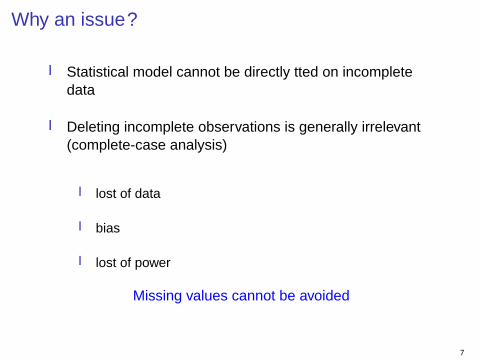
Why an issue?
I Statistical model cannot be directly fitted on incompletedata
I Deleting incomplete observations is generally irrelevant(complete-case analysis)
I lost of data
I bias
I lost of power
Missing values cannot be avoided
7

Outline
Introduction
Modelling with NANotationsSeveral mechanismsChecking assumptions
Handling missing values by imputationSingle imputationMultiple imputation
Others methods
Conclusion
8

Notations and vocabulary
I n: number of individuals
I p: number of variables
I Xn×p: the full data matrix (partially unknown)
I Rn×p : the missing data pattern R = (rij) 1 ≤ i ≤ n1 ≤ j ≤ p
with rij = 1
if xij is missing and 0 otherwise
I xobsi observed profile of the individual i et xmiss
i theunobserved profile
9

Notations and vocabulary (2)
Xn×p, Rn×p, xobsi et xmiss
i can be seen as realisations of randomvariables
I X = (X1, . . . ,Xp): random variables associated to Xn×p
I R = (R1, . . . ,Rp): random variables associated to Rn×p
I X obs and X miss : random variables associated to observedand unobserved parts of X so that X =
(X obs,X miss)
R is called the missing data mechanism
Handling missing values depends on the relationship betweenR and X
10

Several mechanisms
Three kinds of mechanisms (Rubin, 1976; Little, 1995):
I MCAR (missing completely at random)
P(
R|X obs,X miss; γ)
= P (R; γ)
I MAR (missing at random)
P(
R|X obs,X miss; γ)
= P(
R|X obs; γ)
I MNAR (missing not at random)
P(
R|X obs,X miss; γ)6= P
(R|X obs; γ
)
11

Examples
●
●
●
●
●
●
●
● ●
●
●
●
●
●
●
●
●
●
●
●
●
●●
●
●
●
●
●
●
●
●
●
●
●
●
●
●
●
●
●
●
●
●
●
●
●
●
●●
●
●
●
●
●
●
●
●
●
●
●
●
●
●
●
●
●
●
●
●●
●●
●
●
●
●
●
●
●
●
●
●
●
●
●●
●
●
●● ●
●
●
●
●
●
●
●
●
●
●
●●
●
●
●
●
●
●
●
●
●
●
●
●
●
●
●
●
●●
●
●
●●
●●
●
●
●
●
●
●
●
●
●
●
●●●
●
●
●
●
● ●●
●
●
●
●
●
●
●
●
●
●
●
●
●
●
●
●
●
●
●
●
●
●
●
●
●
●
●
●
●
●
●
●
●
●
●
●
●
●
●●
●
●
●
●
●
●
●
●
●
●
●
●
●
●●
●
●
●
●
●
●
●
●
●
●
●
●
●●
●
●
●
●
●
●
●
●
●
●
●
●
●
●
●
●
●
●
●
●
●
●
●
●
●
●
●
●
●
●
●
●
●
●
●
●
●
●
●
●●
●
●
●
●
●
●
●
●
●
●
●
●
●
●
●
●
●
●
●
●
●
●
●
●
●
●
●●
●
●
●
●
●
●
●
●
●
●
●
●
●●
●
●
●●
●
●
●
●
●
●
●
●
●
●
●●
●
●
●
●
●
●
●
●●
●
●
●
●
●
●
●●
●
●
●
●●
●
●
● ●
●
●●●
●
● ●●
●
●
●
●
●
●
●
●
●
●
●
●
●
●
●
●
●
●
●
●
●
●
●
● ●
●
●
●
● ●
●
●
●
●●
●
●
●
●
●
●
●
●
●
●
●
●
●
●
●
●
●
●
●
●
●
●
●
●
●
●
●
●
●
●
●
●
●
●
●
●
●
●
●
●
●
●
●
●
●
●
●
●
●
●
●
●
●
●
●
●
●
●
●
●
●
●
●
●
●
●
●
●
●
●
●
●
●
●
●
●●
●
●
●
●
●
●
●
●
●●
●
●●
●
●
●
●
●
●
●
●
●
●
●●
●
●
●
●
●
●
●
●
●
●
●
●
●
●
−3 −2 −1 0 1 2 3
−4
−2
02
46
Full data
x1
x2
●
●
●
●
● ●
●
●
●
●
●
●
●
●
●
●
●
●
●
●
●
●
●
●
●
●
●
●
●
●
●
●
●
●
●●
●
●
●
●
●
●
●
●
●
●
●
●●
●
●
●●●
●●
●
●
●
●
●
●
●●
●
●●
●
●
●
●
●
●
●●
●
●
●
●
●
●
●
●
●●
●
●
●
●
●
●
●
●●
●
●●
●
●
●
● ●●
●
●
●
●
●
●
●
●
●
●
●
●
●
●
●●
●
●
●
●
●
●
●
●
●
●
●
●
●
●
●
●
●
●
●
●
●
●●
●
●
●
●
●
●
●
●
●
●●
●
●
●
●
●
●
●
●
●
●
●
●
●
●
●
●
●
●
●
●
●
●
●
●
●
●
●
●
●
●●
●
●
●
●
●
●
●
●
●
●
●
●
●
●
●
●●
●
●
●
●
●
●
●
●
●
●
●
●
●
●●
●
●
●
●
●●
●
●
●
●
●
●
●
●
●
●
●
●
●
●
●
●
●
●
●
●
●
●●
●
●
●
●
●
●
●
●
●●
●
● ●
●
●
●
●
●
●
●
●
●
●
●
●
●
●
●
●
●
●
●
●
●
●
●
●
●
●
●
●
●
●
●
●
●
●
●
●
●
●
●
●
●
●
●
●
●
●
●
●
●
●
●
●●
●
●
●
●
●
●●●
●●
●
●
●
●
●
●
●
●
●●
●
●
●
●
●
●
●●
●
●
●
−3 −2 −1 0 1 2 3
−4
−2
02
46
MCAR
x1x2
R = 1 if X2 is missingX1 always observed
P(R = 1|X obs,X miss; γ
)= 0.35
12

Examples
●
●
●
●
●
●
●
● ●
●
●
●
●
●
●
●
●
●
●
●
●
●●
●
●
●
●
●
●
●
●
●
●
●
●
●
●
●
●
●
●
●
●
●
●
●
●
●●
●
●
●
●
●
●
●
●
●
●
●
●
●
●
●
●
●
●
●
●●
●●
●
●
●
●
●
●
●
●
●
●
●
●
●●
●
●
●● ●
●
●
●
●
●
●
●
●
●
●
●●
●
●
●
●
●
●
●
●
●
●
●
●
●
●
●
●
●●
●
●
●●
●●
●
●
●
●
●
●
●
●
●
●
●●●
●
●
●
●
● ●●
●
●
●
●
●
●
●
●
●
●
●
●
●
●
●
●
●
●
●
●
●
●
●
●
●
●
●
●
●
●
●
●
●
●
●
●
●
●
●●
●
●
●
●
●
●
●
●
●
●
●
●
●
●●
●
●
●
●
●
●
●
●
●
●
●
●
●●
●
●
●
●
●
●
●
●
●
●
●
●
●
●
●
●
●
●
●
●
●
●
●
●
●
●
●
●
●
●
●
●
●
●
●
●
●
●
●
●●
●
●
●
●
●
●
●
●
●
●
●
●
●
●
●
●
●
●
●
●
●
●
●
●
●
●
●●
●
●
●
●
●
●
●
●
●
●
●
●
●●
●
●
●●
●
●
●
●
●
●
●
●
●
●
●●
●
●
●
●
●
●
●
●●
●
●
●
●
●
●
●●
●
●
●
●●
●
●
● ●
●
●●●
●
● ●●
●
●
●
●
●
●
●
●
●
●
●
●
●
●
●
●
●
●
●
●
●
●
●
● ●
●
●
●
● ●
●
●
●
●●
●
●
●
●
●
●
●
●
●
●
●
●
●
●
●
●
●
●
●
●
●
●
●
●
●
●
●
●
●
●
●
●
●
●
●
●
●
●
●
●
●
●
●
●
●
●
●
●
●
●
●
●
●
●
●
●
●
●
●
●
●
●
●
●
●
●
●
●
●
●
●
●
●
●
●
●●
●
●
●
●
●
●
●
●
●●
●
●●
●
●
●
●
●
●
●
●
●
●
●●
●
●
●
●
●
●
●
●
●
●
●
●
●
●
−3 −2 −1 0 1 2 3
−4
−2
02
46
Full data
x1
x2
●
●
●
●
●
●
●
●
●
●
●
●
●●
●
●
●
●
●
●
●
●
●
●
●
●
●
●
●
●
●
●
●
●
●
●
●
●
●●
●
●●
●●
●
●
●
●
●
●
●
●
●●
●
●
●
●
●
●
●●
●
●
●
●
●
●
●
●
●
●
●
●
●
●●
●
●
●
●
●●
●
●●●
●
●
●
●
● ●
●
●
●
●
●
●
●
●
●
●
● ●
●
●
●
●
●
●
●
●
●
●
●
●
●
●
●
●
●
●
●
●
●
●
●●
●
●
●
●
●
●
●
●
●
●
●
●
●
●
●
●
●
●
●
●
●
●
●
●
●
●●
●
●
●
●
●●
●
●
●
●
●
●
●
●
●
●
●
●
●
●●
●
●
●
●
●
●
●
●
●
●
● ●
●
●
●
●
●
●
●
●
●
●●
●
●
●●
●
●
●
●
●
●●
● ●
●
●●●
●
●
●
●
●
●
●
●
●
●
●
●
●
●
●
●
●
●
●
●
●
●
● ●
●
●
●●
●
●
●
●
●
●
●●
●
●
●
●
●
●
●
●
●
●
●
●
●
●
●
●
●●
●
●
●
●
●
●
●
●
●
●
●
●
●
●
●
●
●
●
●
●
●
●
●
●
●
●
●
●
●●
●
●
●
●
●
●
●
●
●
●
●
●
●
●
●
● ●
●
●
−3 −2 −1 0 1 2 3
−4
−2
02
46
MAR
x1x2
P(R|X obs,X miss; γ
)= B(Φ(1.2 ∗ xobs − 0.5))
12

Examples
●
●
●
●
●
●
●
● ●
●
●
●
●
●
●
●
●
●
●
●
●
●●
●
●
●
●
●
●
●
●
●
●
●
●
●
●
●
●
●
●
●
●
●
●
●
●
●●
●
●
●
●
●
●
●
●
●
●
●
●
●
●
●
●
●
●
●
●●
●●
●
●
●
●
●
●
●
●
●
●
●
●
●●
●
●
●● ●
●
●
●
●
●
●
●
●
●
●
●●
●
●
●
●
●
●
●
●
●
●
●
●
●
●
●
●
●●
●
●
●●
●●
●
●
●
●
●
●
●
●
●
●
●●●
●
●
●
●
● ●●
●
●
●
●
●
●
●
●
●
●
●
●
●
●
●
●
●
●
●
●
●
●
●
●
●
●
●
●
●
●
●
●
●
●
●
●
●
●
●●
●
●
●
●
●
●
●
●
●
●
●
●
●
●●
●
●
●
●
●
●
●
●
●
●
●
●
●●
●
●
●
●
●
●
●
●
●
●
●
●
●
●
●
●
●
●
●
●
●
●
●
●
●
●
●
●
●
●
●
●
●
●
●
●
●
●
●
●●
●
●
●
●
●
●
●
●
●
●
●
●
●
●
●
●
●
●
●
●
●
●
●
●
●
●
●●
●
●
●
●
●
●
●
●
●
●
●
●
●●
●
●
●●
●
●
●
●
●
●
●
●
●
●
●●
●
●
●
●
●
●
●
●●
●
●
●
●
●
●
●●
●
●
●
●●
●
●
● ●
●
●●●
●
● ●●
●
●
●
●
●
●
●
●
●
●
●
●
●
●
●
●
●
●
●
●
●
●
●
● ●
●
●
●
● ●
●
●
●
●●
●
●
●
●
●
●
●
●
●
●
●
●
●
●
●
●
●
●
●
●
●
●
●
●
●
●
●
●
●
●
●
●
●
●
●
●
●
●
●
●
●
●
●
●
●
●
●
●
●
●
●
●
●
●
●
●
●
●
●
●
●
●
●
●
●
●
●
●
●
●
●
●
●
●
●
●●
●
●
●
●
●
●
●
●
●●
●
●●
●
●
●
●
●
●
●
●
●
●
●●
●
●
●
●
●
●
●
●
●
●
●
●
●
●
−3 −2 −1 0 1 2 3
−4
−2
02
46
Full data
x1
x2
●
●
● ●
●
●
●
●●
●
●
●●
●
●
●
●
●
●
●
●
●
●
●
●
●
●●
●
●
●
●
●
●
●
●
●
●●
●
●
●●
●
●
●
●
●
●
●
●
●
●
●●
●
●
●
●
●
●
●
●
●●
●
●
●
●
●
●
●
●
●
●
●
●
●●
●
●
●●
●
●
●
●
●
●●
●
●
●●●
●
●
●
●
● ●●
●
●
●
●
●
●
●
●
●
●
●
●
●
● ●
●
●
●
●
●
●
●
●
●
●
●
●
●●
●
● ●
●
●
●
●
●
●●
●
●
●
●
●
●
●
●
●
●
●
●
●
●
●
●
●
●
●
●
●
●
●●
●
●
●
●●
●
●
●
●
●
●
●
●
●
●
●
●
●
●
●
●
●
●
●
●
●
●
●
●
●
●●
●
●
●
●
●
●
●
●
●
●●
●
●
●
●
●
●●
●
● ●
●●
● ●
●
●
●
●
●
●
●
●
●
●
●
●
●
●
●
● ●
●
● ●
●
●
●
●●
●
●
●●
●
●
●
●
●
●
●●
●
●
●
●
●
●
●
●
●
●
●
●
●
●
●
●
●
●
●
●
●
●
●
●
●
●
●
●
●
●
●
●
●
●
●
●
●
●
●●
●
●
●
●
●
●
●
●
●
●
●
●
●
● ●
●
●
−3 −2 −1 0 1 2 3
−4
−2
02
46
MNAR
x1x2
P(R|X obs,X miss; γ
)= B(Φ(1.2 ∗ xmiss − 0.5))
12

Reasons of this typology
The type of mechanism is important. For instance, with CCA
I MCAR: complete individuals are representative of the dataset, no issue, except that a part of data is not used
I MAR: complete individuals are generally notrepresentative, inference could be biased
I MNAR: idem. In addition, with only one variable,supplementary assumption should be required...
13

How to identify the type of missing data mechanism?
I statistical test: MCAR vs MAR
I graphical investigations:
I analysis of the missing data pattern (marginal distribution)
I analysis of relationships between R and X obs
14

Analysis of the missing data pattern (1)
max
O3
T9
T12
T15
Ne9
Ne1
2
Ne1
5
Vx9
Vx1
2
Vx1
5
max
O3v
Win
dDire
ctio
n
prop
ortio
n of
mis
sing
s
0
10
20
30
40
Com
bina
tions
max
O3
T9
T12
T15
Ne9
Ne1
2
Ne1
5
Vx9
Vx1
2
Vx1
5
max
O3v
library(VIM)aggr(ozoneNa)
15

Analysis of the missing data pattern (2)
●
−1.0 −0.5 0.0 0.5 1.0 1.5
−1.
0−
0.5
0.0
0.5
1.0
MCA factor map
Dim 1 (19.07%)
Dim
2 (
17.7
1%)
maxO3_m
maxO3_o
T9_m
T9_o
T12_m
T12_o
T15_m
T15_o
Ne9_m
Ne9_o
Ne12_m
Ne12_o
Ne15_m
Ne15_o
Vx9_m
Vx9_o
Vx12_m
Vx12_o
Vx15_m
Vx15_o
maxO3v_m
maxO3v_oWindDirection_o
library(FactoMineR)
pattern<-is.na(ozoneNA)pattern[is.na(ozoneNA)]<-"m"pattern[!is.na(ozoneNA)]<-"o"
res.mca<-MCA(pattern,graph=FALSE)
plot(res.mca,choix="ind",invisible="ind")
16

Analysis of relationships between R and X obs
●
−1.0 −0.5 0.0 0.5 1.0 1.5 2.0
−1.
0−
0.5
0.0
0.5
1.0
1.5
MCA factor map
Dim 1 (11.13%)
Dim
2 (
6.24
%)
maxO3_1
maxO3_2
maxO3_3
maxO3_4
maxO3_NA
T9_1
T9_2
T9_3 T9_4
T9_NA
T12_1
T12_2
T12_3
T12_4
T12_NA
T15_1T15_2
T15_3T15_4
T15_NA
Ne9_1
Ne9_2
Ne9_3Ne9_4 Ne9_NA
Ne12_1
Ne12_2
Ne12_3
Ne12_4
Ne12_NA
Ne15_1Ne15_2
Ne15_3Ne15_4 Ne15_NAVx9_1
Vx9_2
Vx9_3
Vx9_4
Vx9_NA
Vx12_1
Vx12_2 Vx12_3
Vx12_4
Vx12_NA
Vx15_1
Vx15_2Vx15_3
Vx15_4Vx15_NA
maxO3v_1
maxO3v_2
maxO3v_3
maxO3v_4
maxO3v_NA
East
North
South
West
max
O3
T9
T12
T15
Ne9
Ne1
2
Ne1
5
Vx9
Vx1
2
Vx1
5
max
O3v
020
4060
8010
0
Inde
x
don.cat<-ozoneNAquanti<-which(sapply(ozoneNA,is.numeric))for(i in quanti){breaks<-c(-Inf,quantile(don.cat[[i]],na.rm=T)[-1])
don.cat[[i]]<-cut(don.cat[[i]],breaks=breaks,labels=F)
don.cat[[i]]<-addNA(don.cat[[i]],ifany=T)}res.mca<-MCA(don.cat,graph=FALSE)plot(res.mca,choix="ind",invisible="ind")
matrixplot(ozoneNA,sortby=1)
17

Limits of the exploratory analysis
I Exploratory analysis suggests hypothesis
I The relationship with X miss is not known
I A knowledge on data is required to valid the type ofmechanism
18
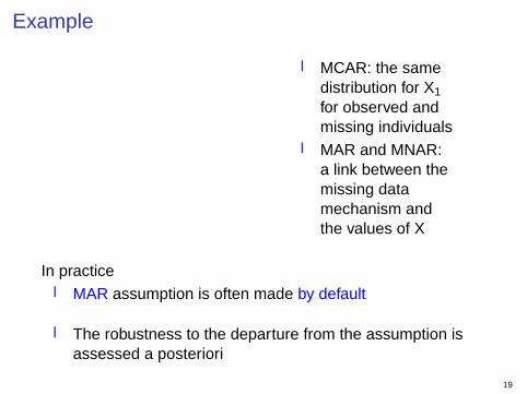
Example
●
●
0 1
−3
−2
−1
01
23
MCAR
R
x_1
●
●
●
0 1
−3
−2
−1
01
23
MAR
R
x_1
●
●
●
0 1
−3
−2
−1
01
23
MNAR
R
x_1
I MCAR: the samedistribution for X1for observed andmissing individuals
I MAR and MNAR:a link between themissing datamechanism andthe values of X
In practiceI MAR assumption is often made by default
I The robustness to the departure from the assumption isassessed a posteriori
19

Outline
Introduction
Modelling with NANotationsSeveral mechanismsChecking assumptions
Handling missing values by imputationSingle imputationMultiple imputation
Others methods
Conclusion
20

Single imputation
I Imputation consists in replacing missing values byplausible values
I Single imputation consists in replacing by one unique value
I ExamplesI mean
I median
I regression
I stochastic regression
I sampling observed data
21

Examples
●
●
●
●
●
●
●●
●
●
●
●
●●
●●
●
●●
●
●
●
●
●
●
●
●
●
●
●
●
●
●
●
●
●
●
●
●●
●
●●●
●
●
●
●
●
●
●
●
●●●
●
●
●
●
●
●
●●
●●
●
●
●
●
●
●
●
●●
●
●
●●
●
●
●
●
●●●
●●●
●
●
●
●
● ●
●
●
●
●
●
●
●
●
●
●
●●
●
●
●●
●
●
●●
●
●
●
●
●
●
●
●
●
●
●
●
●
●
●●
●
●
●
●
●
●
●
●
●
●
●
●●
●
●
●
●●
●●
●
●
●
●
●
●●
●
●
●
●
●●
●
●
●●
●
●
●
●
●
●
●
●
●●●
●
●
●●
●
●
●
●●
●
● ●
●
●
●
●●
●
●
●
●
●●
●
●
●●
●
●
●
●
●
●●
● ●
●
●●●
●
●
●
●
●
●
●●
●
●
●
●
●
●
●
●
●
●
●
●
●
●
● ●
●
●●●
●
●
●
●
●●
●●
●
●
●
●
●
●
●
●
●
●
●
●
●
●
●
●
●●
●
●
●
●
●
●
●
●
●
●
●
●
●
●
●
●
●
●
●
●
●
●
●
●
●
●
●
●
●● ●
●
●
●●
●
●
●
●
●
●
●
●
●●
● ●●
●
−3 −2 −1 0 1 2 3
−4
−2
02
46
mean
x1
x2
●
●
●
●
●
●
●●
●
●
●
●
●●
●●
●
●●
●
●
●
●
●
●
●
●
●
●
●
●
●
●
●
●
●
●
●
●●
●
●●●
●
●
●
●
●
●
●
●
●●●
●
●
●
●
●
●
●●
●●
●
●
●
●
●
●
●
●●
●
●
●●
●
●
●
●
●●●
●●●
●
●
●
●
● ●
●
●
●
●
●
●
●
●
●
●
●●
●
●
●●
●
●
●●
●
●
●
●
●
●
●
●
●
●
●
●
●
●
●●
●
●
●
●
●
●
●
●
●
●
●
●●
●
●
●
●●
●●
●
●
●
●
●
●●
●
●
●
●
●●
●
●
●●
●
●
●
●
●
●
●
●
●●●
●
●
●●
●
●
●
●●
●
● ●
●
●
●
●●
●
●
●
●
●●
●
●
●●
●
●
●
●
●
●●
● ●
●
●●●
●
●
●
●
●
●
●●
●
●
●
●
●
●
●
●
●
●
●
●
●
●
● ●
●
●●●
●
●
●
●
●●
●●
●
●
●
●
●
●
●
●
●
●
●
●
●
●
●
●
●●
●
●
●
●
●
●
●
●
●
●
●
●
●
●
●
●
●
●
●
●
●
●
●
●
●
●
●
●
●● ●
●
●
●●
●
●
●
●
●
●
●
●
●●
● ●●
●
−3 −2 −1 0 1 2 3
−4
−2
02
46
sampling
x1
x2
●
●
●
●
●
●
●●
●
●
●
●
●●
●●
●
●●
●
●
●
●
●
●
●
●
●
●
●
●
●
●
●
●
●
●
●
●●
●
●●●
●
●
●
●
●
●
●
●
●●●
●
●
●
●
●
●
●●
●●
●
●
●
●
●
●
●
●●
●
●
●●
●
●
●
●
●●●
●●●
●
●
●
●
● ●
●
●
●
●
●
●
●
●
●
●
●●
●
●
●●
●
●
●●
●
●
●
●
●
●
●
●
●
●
●
●
●
●
●●
●
●
●
●
●
●
●
●
●
●
●
●●
●
●
●
●●
●●
●
●
●
●
●
●●
●
●
●
●
●●
●
●
●●
●
●
●
●
●
●
●
●
●●●
●
●
●●
●
●
●
●●
●
● ●
●
●
●
●●
●
●
●
●
●●
●
●
●●
●
●
●
●
●
●●
● ●
●
●●●
●
●
●
●
●
●
●●
●
●
●
●
●
●
●
●
●
●
●
●
●
●
● ●
●
●●●
●
●
●
●
●●
●●
●
●
●
●
●
●
●
●
●
●
●
●
●
●
●
●
●●
●
●
●
●
●
●
●
●
●
●
●
●
●
●
●
●
●
●
●
●
●
●
●
●
●
●
●
●
●● ●
●
●
●●
●
●
●
●
●
●
●
●
●●
● ●●
●
−3 −2 −1 0 1 2 3
−4
−2
02
46
regression
x1
x2
●
●
●
●
●
●
●●
●
●
●
●
●●
●●
●
●●
●
●
●
●
●
●
●
●
●
●
●
●
●
●
●
●
●
●
●
●●
●
●●●
●
●
●
●
●
●
●
●
●●●
●
●
●
●
●
●
●●
●●
●
●
●
●
●
●
●
●●
●
●
●●
●
●
●
●
●●●
●●●
●
●
●
●
● ●
●
●
●
●
●
●
●
●
●
●
●●
●
●
●●
●
●
●●
●
●
●
●
●
●
●
●
●
●
●
●
●
●
●●
●
●
●
●
●
●
●
●
●
●
●
●●
●
●
●
●●
●●
●
●
●
●
●
●●
●
●
●
●
●●
●
●
●●
●
●
●
●
●
●
●
●
●●●
●
●
●●
●
●
●
●●
●
● ●
●
●
●
●●
●
●
●
●
●●
●
●
●●
●
●
●
●
●
●●
● ●
●
●●●
●
●
●
●
●
●
●●
●
●
●
●
●
●
●
●
●
●
●
●
●
●
● ●
●
●●●
●
●
●
●
●●
●●
●
●
●
●
●
●
●
●
●
●
●
●
●
●
●
●
●●
●
●
●
●
●
●
●
●
●
●
●
●
●
●
●
●
●
●
●
●
●
●
●
●
●
●
●
●
●● ●
●
●
●●
●
●
●
●
●
●
●
●
●●
● ●●
●
−3 −2 −1 0 1 2 3
−4
−2
02
46
stochastic regression
x1
x2
22

Typology of single imputation methods
I parametric (ex: stochastic regression)I advantages: performs well on small datasetsI drawbacks: sensitive to the model specification
I non-parametric (ex: knn, random forest)I advantages: preserves the nature of the variablesI drawbacks: requires a large number of individuals
I semi-parametric (ex: predictive mean matching)I advantages: preserves the nature of the variables, more
robust to model misspecificationI drawbacks: requires a moderate number of individuals
23

Multivariate imputationWith several missing variables, two strategies:
I Joint modelling1. specify joint distribution for X : P
(X obs,X miss; θ
)Ex: X ∼ Np(µ,Σ), θ = (µ,Σ)
2. estimate θ with missing values with specific algorithm (EM)3. derive the conditional distribution P
(X miss|X obs; θ
)4. draw from the conditional distribution
I Fully Conditional Specification (FCS)1. specify conditional distribution P (Xj |X−j ; θj ) for each
incomplete variable Ex : P (Xj |X−j ) = N (X−jβ,σ2)
2. fill in starting imputations3. for each j
I estimate θj using observed individuals on Xj
I draw missing values of Xj from the conditional distribution
4. repeat 5 to 20 times
24

Joint modelling: pro’s and con’sI Pro’s
I Yield correct statistical inference under the assumed JMI Known theoretical propertiesI Works very well for individuals close to the centerI Often less computationally intensive
I Con’sI Lack of flexibility
I R packagesI normI AmeliaI catI mixI missMDAI jomo
25

FCS: pro’s and con’s
I Pro’sI Very flexibleI EasyI Works well in practice
I Con’sI Theoretical properties generally unknownI Often more computationally intensive than JM
I R packagesI mice, micemd, miceMNARI miI BaboonI VIM
26

Limit of single imputationI Single imputation can lead to unbiased point estimate
●
●
●
●
●
●
●
●
●
●
●
●
●●
●
●
●
●
●
●
●
●
●
●
●
●
●
●
●
●
●
●
●
●
●
●
●
●
●
●
●
●
●
●
●
●
●
●
●
●
●
●
●
●●
●
●
●
●
●
●
●●
●
●
●
●
●
●
●
●
●
●
●
●
●
●●
●
●
●
●
●●
●
●●
●
●
●
●
●
● ●
●
●
●
●
●
●
●
●
●
●
● ●
●
●
●
●
●
●
●
●
●
●
●
●
●
●
●
●
●
●
●
●
●
●
●●
●
●
●
●
●
●
●
●
●
●
●
●
●
●
●
●
●
●
●
●
●
●
●
●
●
●●
●
●
●
●
●●
●
●
●
●
●
●
●
●
●
●
●
●
●
●●
●
●
●
●
●
●
●
●
●
●
● ●
●
●
●
●
●
●
●
●
●
●●
●
●
●●
●
●
●
●
●
●●
● ●
●
●●●
●
●
●
●
●
●
●
●
●
●
●
●
●
●
●
●
●
●
●
●
●
●
● ●
●
●
●●
●
●
●
●
●
●
●
●
●
●
●
●
●
●
●
●
●
●
●
●
●
●
●
●
●●
●
●
●
●
●
●
●
●
●
●
●
●
●
●
●
●
●
●
●
●
●
●
●
●
●
●
●
●
●●
●
●
●
●
●
●
●
●
●
●
●
●
●
●
●
● ●
●
●
−3 −2 −1 0 1 2 3
−4
−2
02
46
stochastic regression
x1
x2
●
●
●●●
●●
●
●●
●
●
●
●●
●
●●●●●●
●●
●●●●
●●
●●●●●●●●●●●●●●●●●●●●●●●●●●●●●●●●●●●●●●●●●●●●●●●●●●●●●●●●●●●●●●●●●●●●●●●●●●●●●●●●●●●●●●●●●●●●●●●●●●●●●●●●●●●●●●●●●●●●●●●●●●●●●●●●●●●●●●●●●
●●●●●●●●●●●●●●●●●●●●●●●●●●●●●●●●●●●●●●●●●●●●●●●●●●●●●●●●●●●●●●●●●●●●●●●●●●●●
●●●●●●●●●●●●●●●●●●●●●●●●●●●●●●●●●●●●●●●●●●●●●●●●●●●●●●●●●●●●●●●●●●●●●●●●●●●●●●●●●●●●●●●●●
●●●●●●●●●●●●●●●●●●●●●●●●●●●●●●●●●●●●●●●●●●●●●●●●●●●●●●●●●●●●●●●●●●●●●●●●●●●●●●●●●●●●●●●●●●●●●●●●●●●●●●●●●●●●●●●●●●●●●●●●●●●●●●●●●●●●●●●●●●●●●●●●●●●●●●●●●●●●●●●●●●●●●●●●●●●●●●●●●●●●●●●●●●●●●●●●●●●●●●●●●●●●●●●●●●●●●●●●●●●●●●●●●●●●●●●●●●●●●●●●●●●●●●●●●●●●●●●●●●●●●●●●●●●●●●●●●●●●●●●●●●●●●●●●●●●●●●●●●●●●●●●●●●●●●●●●●●●●●●●●●●●●●●●●●●●●●●●●●●●●●●●●●●●●●●●●●●●●●●●●●●●●●●●●●●●●●●●●●●●●●●●●●●●●●●●●●●●●●●●●●●●●●●●●●●●●●●●●●●●●●●●●●●●●●●●●●●●●●●●●●●●●●●●●●●●●●●●●●●●●●●●●●●●●●●●●●●●●●●●●●●●●●●●●●●●●●●●●●●●●●●●●●●●●●●●●●●●●●●●●●●●●●●●●●●●●●●●●●●●●●●●●●●●●●●●●●●●●●●●●●●●●●●●●●●●●●●●●●●●●●●●●●●●●●●●●●●●●●●●●●●●●●●●●●●●●●●●●●●●●●●●●●●●●●●●●●●●●●●●●●●●●●●●●●●●●●●●●●●●●●●●●●●●●●●●●●●●●●●●●●●●●●●●●●●●●●●●●●●●●●●●●●●●●●●●●●●●●●●●●●●●●●●●●●●●●●●●●●●●●●●●●●●●●●●●●●●●●●●●●●●●●●●●●●●●●●●●●●●●●●●●●●●●●●●●●●●●●●●●●●●●●●●●●●●●●●●●●●●●●●●●●●●●●●●●●●●●●●●●●●●●●●●●
●●●●●●●●●●●●●●●●●●●●●●●●●●●●●●●●●●●●●●●●●●●●●●●●●●●●●●●●●●●●●●●●●●●●●●●●●●●●●●●●●●●●●●●●●●●●●●●●●●●●●●●●●●●●●●●●●●●●●●●●●●●●●●●●●●●●●●●●●●●●●●●●●●●●●●●●●●●●●●●●●●●●●●●●●●●●●●●●●●●●●●●●●●●●●●●●●●●●●●●●●●●●●●●●●●●●●●●●●●●●●●●●●●●●●●●●●●●●●●●●●●●●●●●●●●●●●●●●●●●●●●●●●●●●●●●●●●●●●●●●●●●●●●●●●●●●●●●●●●●●●●●●●●●●●●●●●●●●●●●●●●●●●●●●●●●●●●●●●●●●●●●●●●●●●●●●●●●●●●●●●●●●●●●●●●●●●●●●●●●●●●●●●●●●●●●●●●●●●●●●●●●●●●●●●●●●●●●●●●●●●●●●●●●●●●●●●●●●●●●●●●●●●●●●●●●●●●●●●●●●●●●●●●●●●●●●●●●●●●●●●●●●●●●●●●●●●●●●●●●●●●●●●●●●●●●●●●●●●●●●●●●●●●●●●●●●●●●●●●●●●●●●●●●●●●●●●●●●●●●●●●●●●●●●●●●●●●●●●●●●●●●●●●●●●●●●●●●●●●●●●●●●●●●●●●●●●●●●●●●●●●●●●●●●●●●●●●●●●●●●●●●●●●●●●●●●●●●●●●●●●●●●●●●●●●●●●●●●●●●●●●●●●●●●●●●●●●●●●●●●●●●●●●●●●●●●●●●●●●●●●●●●●●●●●●●●●●●●●●●●●●●●●●●●●●●●●●●●●●●●●●●●●●●●●●●●●●●●●●●●●●●●●●●●●●●●●●●●●●●●●●●●●●●●●●●●●●●●●●●●●
0 500 1000 1500 2000−0.
10−
0.05
0.00
0.05
0.10
nb sim
y im
p
I However, it is irrelevant for building confidence intervals
●●●●●●●●●●●●●●●●●●●●●●
●●
●
●
●
●●●
●
●
●
●●●●●●●●●●●●●●●●●●●●●●
●●●●●●●●●●●●●●●●●●●●●●●●
●●●●●●●●●●●●●●●●●●●●●●●●●●●●●●●●●●●●●●●●●●●●●●●●●●
●●●●●●●●●●●●●●
●●●●●●●
●●●●●●●●●●●●●●●●●●●●●●●●●●●●●●●●●●●●●●●●●●●●●●●●●●●●●●●●●
●
●●●●●●
●●●●●●●●●
●●●●●●●●●●●
●●●●●●●●
●
●●●●
●●●
●●●●●
●●●●●●●●
●●●●●●●●●●●
●●●●●●●●●●
●●●●●●●●●●●●●●●●●●●●●●●●●●
●●●●●●●●●●●●●●●
●●●●●●●●
●●●●●●●●●●●●●●●●●●●●●●●●●●●●●●●●●●●●●●●●●●●●●●●●●●●●●●●●●●●●●●●●●●●●●●●●●●●●●●●●●●●●●●●●●●●●●●●●●●●●●●●●●●●●●●●●●●●●●●●●●●●●●●●●●●●●●●●●●●●●●●●●●●●●●●●●●●●●●●●●●●●●●●●●●●●●●●●●●●●●●●●●●●●●●●●●●●●●●●●●●●●●●●●●●●●●●●●●●●●●●●●●●●●●●●●●●●●●●●●●●●●●●●●●●●●●●●●●●●●●●●●●●●●●●●●●●●●●●●●●●●●●●●●●●●●●●●●●●●●●●●●●●●●●●●●●●●●●●●●●●●●●●●●●
●●●●●●●●●●●●●●●●●●●●●●●●●●●●●●●●●●●●●●●●●●●●●●●●●●●●●●●●●●●●●●●●●●●●●●●●●●●●●●●●●●●●●●●●●●●●●●●●●●●●●●●●●●●●●●●●●●●●●●●●●●●●●●●●●●●●●●●●●●●●●●●●●●●●●●●●●●●●●●●●●●●●●●●●●
●●●●●●●●●●●●●●●●●●●●●●●●●●●●●●●●●●●●●●●●●●●●●●●●●●●●●●●●●●●●●●●●●●●●
●●●●●●●●●●●●●●●●●●●●●●●●●●●●●●●●●●●●●●●●●●●●●●●●●●●●●●●●●●●●●●●●●●●●●●●●●●●●●●●●●●●●●●●●●●●●●●●●●●●
●●●●●●●●●●●●●●●●●●●●●●●●●●●●●●●●●●●●●●●●●●●●●●●●●●●●●●●●●●●●●●●●●●●●●●●●●●●●●●●●●●●●
●●●●●●●●●●●●●●●●●●●●●●●●●●●●●●●●●●●●●●●●●●●●●●●●●●●●●●●●●●●
●●●●●●●●●●●●●●●●●●●●●●●●●●●●●●●●●●●●●●●●●●●●●●●●●●●●●●●●●●●●●●●●●●●●●●●●●●●●●●●●●●●●●●●●●●●●●●●●●●●●●●●●●●●●●●●●●●●●●●●●●●●
●●●●●●●●●●●●●●●●●●●●●●●●●●●●●●●●●●●●●●●●●●●●●●●●●●●●●●●●●●●●●●●●●●●●●●●
●●●●●●●●●●●●●●●●●●●●●●●●●●●●●●●●●●●●●●●●●●●●●●●●●●●●●●●●●●●●●●●●●●●●●●●●●●●●●●●●●●●●●●●●●●●●●●●●●●●●●●●●●●●●●●●●●●●●●●●●●●●●●●●●
●●●●●●●●●●●●●●●●●●●●●●●●●●●●●●●●●●●●●●●●●●●●●●●●●●●●●●●●●●●●●●●●●●●
●●●●●●●●●●●●●●●●●●●●●●●●●●●●●●●●●●●●●●●●●●●●●●●●●●●●●●●●●●●●●●●●●●●●●●●●●●●●●●●●●●●●●●●●●●●●●●●●●●●●●●●●●●●●●●●●●●●●●●●●●●●●●●●●●●
●●●●●●●●●●●●●●●●●●●●●●●●●●●●●●●●●●●●●●●●●●●●●●●●●●●●●●●●●●●●●●●●●●●●●●●●●●●●●●●●●●●●●●●●●●●●●●●●●●●●●●●●●●●●●●●●●●●●●●●●●●●●●●●●●●●●●●●●●●●●●●●●●●●●●●●●●●●●●●●●●●●●●●●●●●●●●●●●●●●●●●●●●●●●●●●●●●●●●●●●●●●●●●●●●●●●●●●●●●●●●●●●●●●●●●●●●●●●●●●●●●●●●●●●●●●●●●●●●●●●●●●●●●●●●●●●●●●●●●●●●●●●●●●●●●●●●●●●●●●●●●●
●●●●●●●●●●●●●●●●●●●●●●●●●●●●●●●●●●●●●●
0 500 1000 1500 2000
0.90
0.92
0.94
0.96
0.98
1.00
nb sim
covera
ge
27

Multiple imputation (Rubin, 1987)
1. Generate a set of M parameters (θm)1≤m≤M of an imputationmodel to generate M plausible imputed data sets
P(
Xmiss|Xobs,θ1
). . . . . . . . . P
(Xmiss|Xobs,θM
)(F u′)ij (F u′)1ij + ε
1
ij (F u′)2ij + ε2
ij(F u′)3ij + ε
3
ij (F u′)Bij + εBij
2. Fit the analysis model on each imputed data set: βm,Var(βm
)3. Combine the results: β = 1
M
∑Mm=1 βm
Var(β)
= 1M
∑Mm=1 Var
(βm
)+(1 + 1
M
) 1M−1
∑Mm=1
(βm − β
)2
⇒ Provide estimation of the parameters and of their variability
28

Generation of (θm)1≤m≤M
I BayesianI Prior distribution p(θ)I Derive the posterior distribution p(θ|X obs)
(Data-Augmentation)I Draw from p(θ|X obs) M times
I Non-parametric BootstrapI Sampling observations with replacement M timesI Estimate θm from each one (EM)
I Approximate BayesianI For asymptotically Gaussian estimator, estimate mean and
varianceI Draw M values from N
(θ,Var
(θ))
29

Illustration
1. Non-parametric Bootstrap + stochastic regression
●
●
●
●
●
●
●
● ●
●
●
●
●
●
●
●
●
●●
●
●
●
●
●
●
●
●
●●●
●
●
●
●
●●
●
●
●●
●
●
●
●
●
●
●
●●
●
●
●
●
●
●
●
●
●
●
●
●
● ●
●
●
●
●
●
●
●
●
●
●
●
●●
●
●
●
●
●
●
●
●
●
●
●
● ●
●
●
●
●
●
●
●
●
●
●
●
●
●
●
●
●
●
●
●
●
●
●●
●
●
●
●
●
●
●
●
●
●
●
●
●
●
●
●
●
●
●
●
●
●
●
●
●
●
●
●
●
●
●
●
●
●
●
● ●
●
●
●
●
●●
●
●
●
●
●
●
●●●
●
●
●
●
●
●
●
●
●
●
●●
●
●
● ●
●
●
●●●
●
● ●●
●
●
●
●
●
●
●
●
●
●●
●
●
●
●
●
●
●
●
●●
●
●●
●
●
●
●
●
●
●
●
●
●
●
●
●
●
●
●
●
●
●
●
●
●
●
●●
●
●
●
●
●
●
●
●
●
●
●
●
●
●
●
●
●●
●
●
●
●●
●
●
●
●●
●
●
●
●
●
●
●
●
●
●
●
●
●
●
●
●
●
●
●
●
●
●
●
●
●
●●
●
●
●
●
●
●
●
●
●
●
●
●
●
●
●
●
●
●
●
●
●
●
●
●
●
●●
●
−3 −2 −1 0 1 2 3
−4
−2
02
46
m=1
x
y
●
●
●
●
●
●
●
●
●●
●
●
●
●
●
●
●
●
●
●
●
●
●
●
●
●
●
●
●●
●
●
●
●
●●
●
●
●
●
●
●
●
●
●
●
●
●●
●
●
●
●
●
●
●
●
●
●●
●
● ●
●
●
●
●
●
●
●
●
●
●
●
●●
●
●
●
●
●
●
●
●
●
●
●
● ●
●
●
●
●
●
●
●
●
●
●
●
●
●
●
●
●
●
●
●
●
●
●●
●
●
●
●
●
●
●
●
●
●
●
●
●
●
●
●
●
●
●
●
●
●
●
●
●
●
●
●
●
●
●
●
●
●
●
● ●
●
●
●
●
●●
●
●
●
●●
● ●●●
●
●
●
●
●
●●
●
●
●●
●
●
●
● ●
●
●
●●●
●
●
●
●
●
●
●
●
●
●
●
●
●
●●
●
●
●
●
●
●
●
●
●
●
●
●
●
●
●
●
●
●
●
●
●
●
●
●
●
●
●
●
●
●
●
●
●
●
●
●
●●
●
●
●
●
●
●
●
●
●
●
●
●
●
●
●
●
●
●
●
●
●
●●
●
●●
●●
●
●
●
●
●
●
●
●
●
●
●
●●
●
●
●
●
●
●
●
●
●
●
●
●
●
●
●
●
●
●
●
●
●
●
●
●
●
●
●
●
●●
●
●
●
●
●
●
●
●
●
●
●
●
−3 −2 −1 0 1 2 3
−4
−2
02
46
m=2
x
y
●
●
●
●
●
●
●
●
●
●
●
●
●
●
●
●
●
●
●
●
●
●
●
●
●
●
●
●
●●
●
●
●
●
●●
●
●
●
●
●
●
●
●
●
●●
●●
●
●
●
●
●
●
●
●
●
●
●
●
● ●
●
●
●
●
●
●
●
●
●
●
●
●●
●
●
●
●
●
●
●
●
●
●
●
● ●
●
●
●
●
●
●●
●
●
●
●
●
●
●
●
●
●
●
●
●
●
●
●
●
●
●
●
●
●
●
●
●
●
●
●
●
●
●
●
●
●
●
●
●
●
●
●
●
●
●
●
●
●
●
●
●
●
●
● ●
●
●
●
●
●●
●
●
●
●
●
●●
●
●
●
●
●
●
●
●
●
●
●
●
●●
●
●
● ●
●
●
●●●
●
●
●
●
●
●
●
●
●
●
●
●
●
●●
●
●
●
●
●
●
●
●
●
●
●
●
●
●●
●
●
●
●
●
●
●
●
●
●
●
●
●
●
●
●
●
●
●
●
●
●●
●
●
●
●
●
●
●
●
●
●
●
●●
●
●
●
●●
●
●
●
●● ●●
●
●
●
●
●
●
●
●
●
●●
●
●●
●
●
●
●
●
●
●
●
●
●
●
●
●
●
●●
●
●
●
●
●
●
●
●
●
●
●
●
●
●
●
●
●
●
●
●
●
●
●
●
●
● ●
●
−3 −2 −1 0 1 2 3
−4
−2
02
46
m=3
x
y
library(mice)res.mice<-mice(don,m=3,method="norm.boot")
2. Estimate β = E(Y ) and Var(β) from each imputed tableres.with<-with(res.mice,lm(y~1))
3. Aggregate resultspool(res.with)
30

Illustration: quality of the inference
●
●
●
●
●
●
●
●
●●●●●●●●
●●●
●●●●●●●●●●●●●●●●●●●●●●●●●●●●●●●●●●●●●●●●●●●●●●●●●●●●●●●●●●●●●●●●●●●●●●●●●●●●●●●●●●●●●●●●●●●●●●●●●●●●●●●●●●●●●●●●●●●●●●●●●●●●●●●●●●●●●●●●●●●●●●●●●●●●●●●●●●●●●●●●●
●●●●●●●●●●●●●●●●●●●●●●●●●●●●●●●●●●●●●●●●●●●●●●●●●●●●●●●●●●●●●●●●●●●●●●●●●●●●●●●●
●●●●●●●●●●●●●●●●●●●●●●●●●●●●●●●●●●●●●●●●●●●●●●●●●●●●●●●●●●●●●●●●●●●●●●●●●●●●●●●●●●●●●●●●●●●●●●●●●●●●●●●●●●●●●●●●●●●●●●●●●●●●●●●●●●●●●●●●●●●●●●●●●●●●●●●●●●●●●●●●●●●●●●●●●●●●●●●●●●●●●●●●●●●●●●●●●●●●●●●●●●●●●●●●●●●●●●●●●●●●●●●●●●●●●●●●●●●●●●●●●●●●●●●●●●●●●●●●●●●●●●●●●●●●●●●●●●●●●●●●●●●●●●●●●●●●●●●●●●●●●●●●●●●●●●●●●●●●●●●●●●●●●●●●●●●●●●●●●●●●●●●●●●●●●●●●●●●●●●●●●●●●●●●●●●●●●●●●●●●●●●●●●●●●●●●●●●●●●●●●●●●●●●●●●●●●●●●●●●●●●●●●●●●●●●●●●●●●●
●●●●●●●●●●●●●●●●●●●●●●●●●●●●●●●●●●●●●●●●●●●●●●●●●●●●●●●●●●●●●●●●●●●●●●●●●●●●●●●●●●●●●●●●●●●●●●●●●●●●●●●●●●●●●●●●●●●●●●●●●●●●●●●●●●●●●●●●●●●●●●●●●●●●●●●●●●●●●●●●●●●●●●●●●●●●●●●●●●●●●●●●●●●●●●●●●●●●●●●●●●●●●●●●●●●●●●●●●●●●●●●●●●●●●●●●●●●●●●●●●●●●●●●●●●●●●●●●●●●●●●●●●●●●●●●●●●●●●●●●●●●●●●●●●●●●●●●●●●●●●●●●●●●●●●●●●●●●●●●●●●●●●●●●●●●●●●●●●●●●●●●●●●●●●●●●●●●●●●●●●●●●●●●●●●●●●●●●●●●●●●●●●●●●●●●●●●●●●●●●●●●●●●●●●●●●●●●●●●●●●●●●●●●●●●●●●●●●●●●●●●●●●●●●●●●●●●●●●●●●●●●●●●●●●●●●●●●●●●●●●●●●●●●●●●●●●●●●●●●●●●●●●●●●●●●●●●●●●●●●●●●●●●●●●●●●●●●●●●●●●●●●●●●●●●●●●●●●●●●●●●●●●●●●●●●●●●●●●●●●●●●●●●●●●●●●●●●●●●●●●●●●●●●●●●●●●●●●●●●●●●●●●●●●●●●●●●●●●●●●●●●●●●●●●●●●●●●●●●●●●●●●●●●●●●●●●●●●●●●●●●●●●●●●●●●●●●●●●●
●●●●●●●●●●●●●●●●●●●●●●●●●●●●●●●●●●●●●●●●●●●●●●●●●●●●●●●●●●●●●●●●●●●●●●●●●●●●●●●●●●●●●●●●●●●●●●●●●●●●●●●●●●●●●●●●●●●●●●●●●●●●●●●●●●●●●●●●●●●●●●●●●●●●●●●●●●●●●●●●●●●●●●●●●●●●●●●●●●●●●●●●●●●●●●●●●●●●●●●●●●●●●●●●●●●●●●●●●●●●●●●●●●●●●●●●●●●●●●●●●●●●●●●●●●●●●●●●●●●●●●●●●●●●●●●●●●●●●●●●●●●●●●●●●●●●●●●●●●●●●●●●●●●●●●●●●●●●●●●●●●●●●●●●●●●●●●●●●●●●●●●●●●●●●●●●●●●●●●●●●●●●●●●●●●●●●●●●●●●●●●●●●●●●●●●●●●●●●●●●●●●●●●●●●●●●●●●●●●●●●●●●●●●●●●●●●●●●●●●●●●●●●●●●●●●●●●●●●●●●●●●●●●●●●●●●●●●●●●●●●●●●●●●●●●●●●●●●●●●●●●●●●●●●●●●●●●●●●●●●●●●●●●●●●●●●●●●●●●●●●●●●●●●●●●●●●●●●●●●●●●●●●●●●●●●●●●●●●●●●●●●●●●●●●●●●●●●●●●●●●●●●●
0 500 1000 1500 2000−0.
10−
0.05
0.00
0.05
0.10
nb sim
y im
p
●●●●●●●●●●●●●●●●●●●
●●●●●●●●●●●●●●●●●●●●●●●●●●●●●●●
●●●●●●●●●●●●●●●●●●●●●
●●●●●●●
●●●●●●●●●●●●●●●●●●●●●●●●●●●●●●●●●●●●●●●●●●●●●●●●●●●●●●●●●●●●
●●●●●●●●●●●●●●●●●
●●●
●●●●●●●●●●●
●●●●●●●●●●●
●●●●●●●●●●●●●●●●●
●●●●●●
●●●●●●●●●●●●●●●●●●●●●●●●●●●●●
●●●
●●●●●●●●●●●●
●●●●●●●●●●
●●●●●●●●●●●●●●●●●●●●●●●●●●●●●●●
●●●●●●●●
●●●●●●●●●●●●●●●●●●●●●●●●
●●●●●●●●●●●●●●●●●●
●●●●●●●●●●●●●●●●●●●●●●●●●●●●●●●●●●●●●●●●●●●●●●●●●●●●●●●●●●●●●●●●●●●●●●●●●●●●●●●●●●●●●●●●●●●●●●●●●●●●●●●●●●●●●●●●●●●●●●●●●●●●●●●●●●●●●●●●●●●●●●●●●●●●●●●●●●●●●●●●●●●●●●●●●●●●●●●●●●●●●●●●●●●●●●●●●●●●●●●●●●●●●●●●●●●●●●●●●●●●●●●●●●●●●●●●●●●●●●●●●●●●●●●●●●●●●●●●●●●●●●●●●●●●●●●●●●●●●●●●●●●●●●●●●●●●●●●●●●●●●●●●●●●●●●●●●●●●●●●●●●●●●●●●●●●●●●●●●●●●●●●●●●●●●●●●●●●●●●●●●●●●●●●●●●●●●●●●●●●●●●●●●●●●●●●
●●●●●●●●●●●●●●●●●●●●●●●●●●●●●●●●●●●●●●●●●●●●●●●●●●●●●●●●●●●●●●●●
●●●●●●●●●●●●●●●●●●●●●●●●●●●●●●●●●●●●●●●●●●●●●●●●●●●●●●●●●●●●●●●●●●●●●●●●●●●●●●●●●●
●●●●●●●●●●●●●●●●●●●●●●●●●●●●●●●●●●●●●●●●●●●●●●●●●●●●●●●●●●●●●●●●●●●●●●●●●●●●●●●●●●●●●
●●●●●●●●●●●●●●●●●●●●●●●●●●●●●●●●●●●●●●●●●●●●●●●●●●●●●●●●●●●●
●●●●●●●●●●●●●●●●●●●●●●●●●●●●●●●●●●●●●●●●●●●●●●●●●●●●●●●●●●●●●●●●●●●●●●●●●●●●●●●●●●●●●
●●●●●●●●●●●●●●●●●●●●●●●●●●●●●●●●●●●●●●●●●●●●●●●●●●●●
●●●●●●●●●●●●●●●●●●●●●●●●●●●●●●●●●●●●●●●●●●●●●●●●●●●●●●●●●●●●●●●●●●●●●●●●●●●●●●●●●●●●●●●●●●●●●●●●●●●●●●●●●●●●●●●●●●●●●●●●●●●●●●●●●●●●●●●●●●●●●●●●●●●●●●●●●●●●●●●●●●●●●●●●●●●●●●●●●
●●●●●●●●●●●●●●●●●●●●●●●●●●●●●●●●●●●●●●●●●●●●●●●●●●●●●●●●●●●●●●●●●●●●●●●●●●●●●●●●●●●●●●●●●●●●●●●●●●●●●●●●●●●●●●●●●●●●●●●●●●●●●●●●●●●
●●●●●●●●●●●●●●●●●●●●●●●●●●●●●●●●●●●●●●●●●●●●●●●●●●●●●●●●●●●●●●●●●●●●●●●●●●●●●●●●●●●●●●●●●●●●●●●●●●●●●●●●●●●●●●●●●●●●●●●●●●●●●●●●●●●●●●●●●●●●●●●●●●●●●●●●●●●
●●●●●●●●●●●●●●●●●●●●●●●●●●●●●●●●●●●●●●●●●●●●●●●●●●●●●●●●●●●●●●●●●●●●●●●●●●●●●●●●●●●●●●●●●●●●●●●●●●●●●●●●●●●●●●●●●●●●●●●●●●●●●●●●●●●●●●●●●●●●●●●●●●●●●●●●●●●●●●●●●●●●●●●●●●●●●●●●●●●●●●●●●●●●●●●●●●●●●●●●●●●●●●●●●●●●●●●●●●●●●●●●●●●●●●●●●●●●●●●●●●●●●●●●●●●●●●●●●●●●●●●●●●●●●●●●●●●●●●●●●●●●●●●●●
●●●●●●●●●●●●●●●●●●●●●●●●●●●●●●●●●●●●●●●●●●●●●●●●●●●●●●●●●●●●●●●●●●●●●●●●●●●●●●●●●●●●●●●●●●●
0 500 1000 1500 2000
0.90
0.92
0.94
0.96
0.98
1.00
nb simco
vera
ge
FIG.: Point estimate and coverage according to the number ofsimulations
31

How many imputed tables?I Confidence intervals are valid and inference unbiased for
M ≥ 2I Large value for M is more time consumingI M modifies the width of the confidence intervalI In practice, M between 5 and 100
●
●
●
●
●
●●
●●
● ● ● ● ● ● ● ● ● ● ● ● ● ● ● ● ● ● ● ●
5 10 15 20 25 300.34
6263
50.
3462
635
0.34
6263
50.
3462
635
0.34
6263
5
(Intercept)
m
95%
CI w
idth
library(micemd)
res.mice<-mice.par(don,m=30,method="norm.boot",nnodes = 8)
res.with<-with(res.mice,lm(y~1))plot(res.with)
32

Model fitting
−6 −4 −2 0 2 4 6
0.00
0.05
0.10
0.15
0.20
0.25
Observed and imputed values for x_2D
ensi
ty
observedimputed
−6 −4 −2 0 2 4
−8
−6
−4
−2
02
4
Observed versus imputed values for x_2
Observed Values
Impu
ted
Val
ues
0−.2 .2−.4 .4−.6 .6−.8 .8−1
FIG.: Comparative distributions and overimputation
res.mice<-mice.par(don,m=200,nnodes = 8)overimpute(res.mice)
33

Sensitivity analysis
I Aim: assess the robustness to a departure from the MARassumption
I Principle: shift a conditional distribution and look atconsequences on other imputed values
I Method (for FCS):1. choose an incomplete variable2. define a grid of scalars δ (e.g. : 0,.5,1,2)3. add systematically delta to all imputed values of the variable4. explore the modifications on the other imputed values
I see:http://www.gerkovink.com/miceVignettes/Sensitivity_analysis/Sensitivity_analysis.html
34

Good practices
I start by exploratory analysis
I choose an imputation in line with the analysis model
I include a large number of variables
I check the convergence of the algorithms used forimputation
I check the fit of the imputation model
I use a large number of tables for reproducibility
I make sensitivity analysis I would prefer a carefully constructedimputation model (which is based on all available data) over a poorlyconstructed sensitivity analysis (van Buuren, 2012)
35

Limits of MI
I Congeniality: the analysis model and the imputation modelshould be derived from a unique joint distribution (Schafer,2003)
I Rubin rules: all parameters cannot be pooled (Marshallet al., 2009)
I Specific data structure: time series, hierarchical data,constraint,...
I Big data
36

Outline
Introduction
Modelling with NANotationsSeveral mechanismsChecking assumptions
Handling missing values by imputationSingle imputationMultiple imputation
Others methods
Conclusion
37

Others methods
I Direct inference by frequentist or Bayesian approachesI Should be better
I However, not always feasible
I Specific to the analysis model
I Weighting methodsI No variability on the weights
I Tricky with models including several incomplete variables
38

ConclusionI The idea of imputation is both seductive and dangerous. It
is seductive because it can lull the user into thepleasurable state of believing that the data are completeafter all, and it is dangerous because it lumps togethersituations where the problem is sufficiently minor that it canbe legitimately handled in this way and situations wherestandard estimators applied to the real and imputed datahave substantial biases. (Dempster and Rubin, 1983)
I Single imputation aims to complete a dataset as best aspossible. Multiple imputation aims to perform otherstatistical methods after and to estimate parameters andtheir variability taking into account the missing valuesuncertainty.
I MI is one way to deal with missing values, but probably themost popular
39

References I
D. B. Rubin. Inference and missing data. Biometrika, 63:581–592, 1976.R. J. A. Little. Modelling the drop-out mechanism in repeated measures studies.
Journal of the American Statistical Association, 90:1112–1121, 1995.D. B. Rubin. Multiple Imputation for Non-Response in Survey. Wiley, New-York, 1987.S. van Buuren. Flexible Imputation of Missing Data (Chapman & Hall/CRC
Interdisciplinary Statistics). Chapman and Hall/CRC, 2012.J. L. Schafer. Multiple imputation in multivariate problems when the imputation and
analysis models differ. Statistica Neerlandica, 57(1):19–35, 2003.A. Marshall, D. G. Altman, R. L. Holder, and P. Royston. Combining estimates of
interest in prognostic modelling studies after multiple imputation: current practiceand guidelines. Bmc Medical Research Methodology, 9(5):57, 2009.
J. L. Schafer. Analysis of Incomplete Multivariate Data. Chapman & Hall/CRC, London,1997.
factominer.free.fr/missMDA/appendix_These_Audigier.pdf
http://www.stefvanbuuren.nl/mi/docs/MNAR.pdf
http://www.stefvanbuuren.nl/mi/Software.html
40